Feature-Oriented Regional Modeling and Simulations (FORMS) In the Gulf of Maine and Georges Bank

Avijit Gangopadhyay

The School for Marine Science and Technology and Department of Physics

University of Massachusetts at Dartmouth

706 Rodney French Blvd, New Bedford, MA 02744

(Corresponding Author) Fax: (508) 999-9115.

Email: avijit@umassd.edu

Allan R. Robinson

Patrick J. Haley Wayne G. Leslie Carlos J. Lozano

Division of Engineering and Applied Sciences

Harvard University

29 Oxford Street, Cambridge, MA 02138

James J. Bisagni and Zhitao Yu

The School for Marine Science and Technology

University of Massachusetts at Dartmouth

706 Rodney French Blvd, New Bedford, MA 02744

Accepted for publication

CONTINENTAL SHELF RESEARCH

August 14, 2002

1

Table of Contents 1 Introduction................................................................................................................ 3 2 Prevalent features and modeling domains for coastal GOMGB........................ 6 3 Temperature-Salinity Feature Models (TSFMs).................................................... 8

3.1 A general formulation......................................................................................... 8 3.2 The Maine Coastal Current (MCC) ................................................................... 9 3.3 The Shelf-Slope Front (SSF) .............................................................................. 11 3.4 Fronts around Georges Bank............................................................................ 12 3.5 Channel Inflow and Outflow ........................................................................... 14 3.6 The Cyclonic Gyres in the interior Gulf.......................................................... 15

3.6.1 The Jordan and Georges Basin Gyres...................................................... 16 3.6.2 The Wilkinson Basin Gyre ........................................................................ 17

4 Construction of synoptic realizations................................................................... 17 4.1 Development of a synoptic feature-oriented circulation template............. 18 4.2 Feature-oriented initialization for the shelf-slope coastal ocean................. 19

5 Dynamical Simulations........................................................................................... 22 5.1 Model Computational Parameters .................................................................. 22 5.2 Simulations in the GOMGB without atmospheric forcing........................... 24 5.3 Simulations in the GOM with atmospheric forcing...................................... 25

6 Summary and Conclusion...................................................................................... 27

2

Abstract

The multi-scale synoptic circulation system in the Gulf of Maine and Georges Bank (GOMGB) region is presented using a feature-oriented approach. Prevalent synoptic circulation structures, or ‘features,’ are identified from previous observational studies. These features include the buoyancy-driven Maine Coastal Current (MCC), the Georges Bank anticyclonic frontal circulation system, the basin-scale cyclonic gyres (Jordan, Georges and Wilkinson), the deep inflow through the Northeast Channel (NEC), the shallow outflow via the Great South Channel (GSC), and the shelf-slope front (SSF). Their synoptic water-mass (t-s) structures are characterized and parameterized in a generalized formulation to develop temperature-salinity feature models. A synoptic initialization scheme for feature-oriented regional modeling and simulation (FORMS) of the circulation in the coastal-to-deep region of the GOMGB system is then developed. First, the temperature and salinity feature-model profiles are placed on a regional circulation template and then objectively analyzed with appropriate background climatology in the coastal region. Furthermore, these fields are melded with adjacent deep-ocean regional circulation (Gulf Stream Meander and Ring region) along and across the shelf-slope front. These initialization fields are then used for dynamical simulations via the primitive equation model. Simulation results are analyzed to calibrate the multi-parameter feature-oriented modeling system. Experimental short-term synoptic simulations are presented for multiple resolutions in different regions with and without atmospheric forcing. The presented ‘generic and portable’ methodology demonstrates the potential of applying similar FORMS in many other regions of the Global Coastal Ocean.

3

1 Introduction Every oceanic region is unique in its dynamic behavior, which can be expressed in terms of the evolution and interaction of prevalent structures over many scales, although the structures are generic. Such characterization involves various oceanographic properties, as they relate to these specific structures. Linking the features by kinematics and dynamics helps describe the circulation of the regional system. Thus, regional multiscale feature models should be first made kinematically consistent with respect to mass conservation. Also, they may be adjusted to geostrophy, tidal driving and topography. The resulting circulation model provides a general synthesis of the regional coastal circulation and serves as an efficient basis to characterize the synoptic state of the region. A feature-oriented circulation model was developed for the Gulf Stream Meander and Ring (GSMR) region and was described as ‘Multiscale Feature Models (MSFM)’ (Gangopadhyay et al., 1997). A set of multiscale features for the GSMR include the large-scale Gulf Stream, which is mesoscale in its meandering and ring formation; the sub-basin scale recirculation gyres; and the Deep Western Boundary Current (DWBC). Insertion of kinematically synthesized features into a numerical primitive equation model dynamically adjusts the features and provides the basis for a multi-parameter sensitivity study. The Gangopadhyay et al. (1997) circulation model was calibrated for realistic meandering wavegrowth and ring formation via a systematic sensitivity study by Robinson and Gangopadhyay (1997), which was further validated against real case studies by Gangopadhyay and Robinson (1997). Knowledge-based “feature models” have been used for regional simulations and operational forecasting for the past two decades. Specifically, the studies by Robinson, Spall and Pinardi (1988), Robinson et al. (1989), Spall and Robinson (1990), Fox et al. (1992), Glenn and Robinson (1995), Hurlburt et al. (1996), Cummings et al. (1997), Gangopadhyay et al. (1997) and Robinson and Glenn (1999) have applied the “feature-modeling technique” for use in nowcasting, forecasting and assimilation of various in situ (XBT, CTD) and satellite (GEOSAT, Topex/Poseidon) observations in the western North Atlantic. A significant focus was on the meanders and rings of the Gulf Stream system, and some of these operational systems have shown significant success, as opposed to persistence, in predicting the behavior of the ring-stream system on 1-2 week period (Glenn and Robinson, 1995; Gangopadhyay and Robinson, 1997). Other applications include (1) operational implementation by the Royal Navy (Heathershaw and Foreman, 1996), (2) global application in a coupled ocean-atmosphere climate prediction mode (Johns et al., 1997), and (3) process studies in the Gulf Stream trough formation (Gangopadhyay and Lindstrom, 2002).

4

Gangopadhyay and Robinson (2002) (hereafter, GR02) presented a generalized formulation for this approach. The generalization can be summarized as a three- step procedure. First, a regional synoptic feature-oriented circulation template is developed via a synthesis of past observational studies in the region. Second, individual feature models for each of the features are developed from similar studies. Finally, the feature model profiles on the template locations are objectively analyzed with appropriate background climatology to result in a three-dimensional synoptic realization ready for model applications. The multiscale feature oriented regional methodology provides (1) a dynamically balanced regional climatology that maintains the synoptic structures of the system, (2) synoptic fields for initialization and updating for nowcasting, forecasting and assimilation, and (3) calibration and validation of both physical and coupled inter-disciplinary models. The purpose of this study is twofold: (1) to describe the synoptic features of the coastal system of the GOMGB region that are relevant primarily for synoptic and secondarily for seasonal-to-interannual variability; (2) to represent and parameterize such a system for application to nowcasting/forecasting and the assimilation of data/features, which includes melding of synoptic states of the slope and GSMR region with the shelf regions (e.g., GOMGB) in the western north Atlantic. Coastal ocean modeling remains a challenge due to the complexity of the many processes in these regions and a poor understanding of the issues involving model implementation and behavior (Haidvogel and Beckmann, 1998). Modeling studies for the GOMGB region have traditionally focused on reproducing seasonal variability in the Gulf (Lynch et al., 1992, Naimie, 1995, Xue, 2000), tidal modeling (Chen and Beardsley, 1995), and wind-driven climatological studies (Brown, 1998a). Recent studies have also looked at short-term multidisciplinary forecasting and assimilation (McGillicuddy et al., 1998) focused primarily on the winter-spring bloom on the Georges Bank. We focus on synoptic modeling of the physical variability in this coastal region. An interdisciplinary ocean prediction system was developed and described by Robinson (1996). The system uses the Harvard Ocean Prediction System (HOPS) for practical, real-time, regional forecasting and nowcasting (Robinson and Leslie, 1985; Robinson et al., 1995). HOPS is being used in many parts of the world ocean for synoptic forecasting. Its coastal applications are highlighted by Robinson (1999). We present here, a feature-oriented approach, which is useful for understanding issues related to short-term synoptic forecasting and assimilation over the GOMGB region.

5

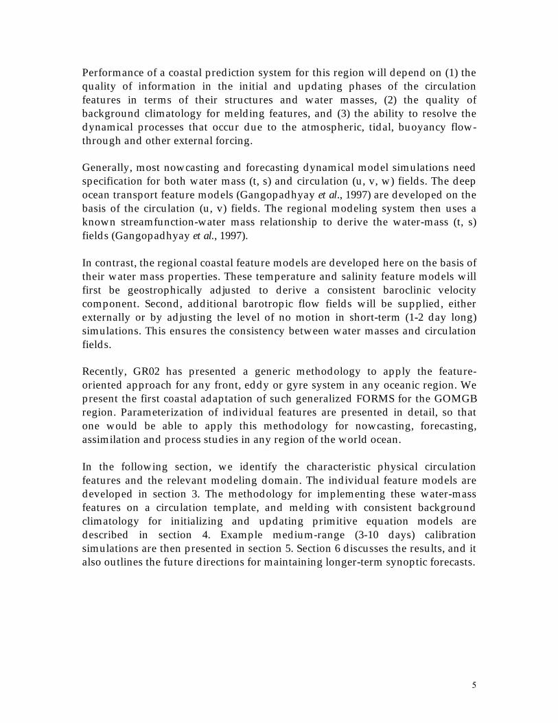
Performance of a coastal prediction system for this region will depend on (1) the quality of information in the initial and updating phases of the circulation features in terms of their structures and water masses, (2) the quality of background climatology for melding features, and (3) the ability to resolve the dynamical processes that occur due to the atmospheric, tidal, buoyancy flow-through and other external forcing. Generally, most nowcasting and forecasting dynamical model simulations need specification for both water mass (t, s) and circulation (u, v, w) fields. The deep ocean transport feature models (Gangopadhyay et al., 1997) are developed on the basis of the circulation (u, v) fields. The regional modeling system then uses a known streamfunction-water mass relationship to derive the water-mass (t, s) fields (Gangopadhyay et al., 1997). In contrast, the regional coastal feature models are developed here on the basis of their water mass properties. These temperature and salinity feature models will first be geostrophically adjusted to derive a consistent baroclinic velocity component. Second, additional barotropic flow fields will be supplied, either externally or by adjusting the level of no motion in short-term (1-2 day long) simulations. This ensures the consistency between water masses and circulation fields. Recently, GR02 has presented a generic methodology to apply the feature-oriented approach for any front, eddy or gyre system in any oceanic region. We present the first coastal adaptation of such generalized FORMS for the GOMGB region. Parameterization of individual features are presented in detail, so that one would be able to apply this methodology for nowcasting, forecasting, assimilation and process studies in any region of the world ocean. In the following section, we identify the characteristic physical circulation features and the relevant modeling domain. The individual feature models are developed in section 3. The methodology for implementing these water-mass features on a circulation template, and melding with consistent background climatology for initializing and updating primitive equation models are described in section 4. Example medium-range (3-10 days) calibration simulations are then presented in section 5. Section 6 discusses the results, and it also outlines the future directions for maintaining longer-term synoptic forecasts.

6

2 Prevalent features and modeling domains for coastal GOMGB The GOMGB region is comprised of a semi-enclosed basin in the Gulf of Maine (GOM) and an offshore submarine bank on Georges Bank (GB). Its large-scale circulation is influenced by buoyancy driving, bottom topography, tides, river inflow, atmospheric forcing, and basin-wide pressure gradient set-up (Bigelow, 1927; Loder, 1980; Brown and Irish, 1992; Brown and Irish, 1993; Loder et al., 1998). A major feature is the narrow Maine Coastal Current (MCC), with its bifurcating and trifurcating segments. The MCC has been the subject of many observational and modeling studies (Bisagni et al., 1996; Pettigrew et al., 1998; Lynch, 1999, Xue et al., 2000). The deep basin regions are dominated by topographically controlled cyclonic gyres: the Georges Basin gyre, the Jordan Basin gyre and the Wilkinson Basin circulation. The two smaller gyres on the Georges and Jordan basins have deep cores within an elliptical outer region. The circulation over the Wilkinson basin, however, is less clearly defined as a single gyre in the stratified season, probably due to the fragmented topography underneath. It is also a major region of vertical mixing in the winter (Brown and Irish, 1993). The saline water enters from the slope through the deeper Northeast Channel (NEC). A major part of the outflow from the GOM domain occurs through the relatively shallow GSC, in addition to the around-the-Bank circulation. In the southern part of the GOMGB region and the northern part of the GSMR region is the Slope water region, where the prevalent flow is towards the southwest. However, the Warm Core Rings (WCRs) are present in this background circulation, which affects the regional circulation considerably. This salty Slope water region creates a water-mass boundary with the fresher GOMGB circulation system along a narrow region close to the 100m isobath, which is known as the shelf-break or the shelf-slope front (SSF). The shallow Georges Bank is a region of tidal influence, modified by the GOM circulation along the northern flank and by the SSF along its southern flank. The tidal front locations follow the classic constraints posed by the depth-dissipation criterion (Simpson and Hunter, 1974; Loder and Greenberg, 1986). Specifically, there appears to be two frontal regions in the southern side along the 60m and the 100m isobaths, and there is also one along the northern edge (50m isobath). The shallowest region on the crest of the bank is well mixed during both summer and winter seasons. Thus, we characterize this regional circulation by five important circulation features: (i) the Maine Coastal Current (MCC), (ii) the shelf-slope front (SSF), (iii)

7

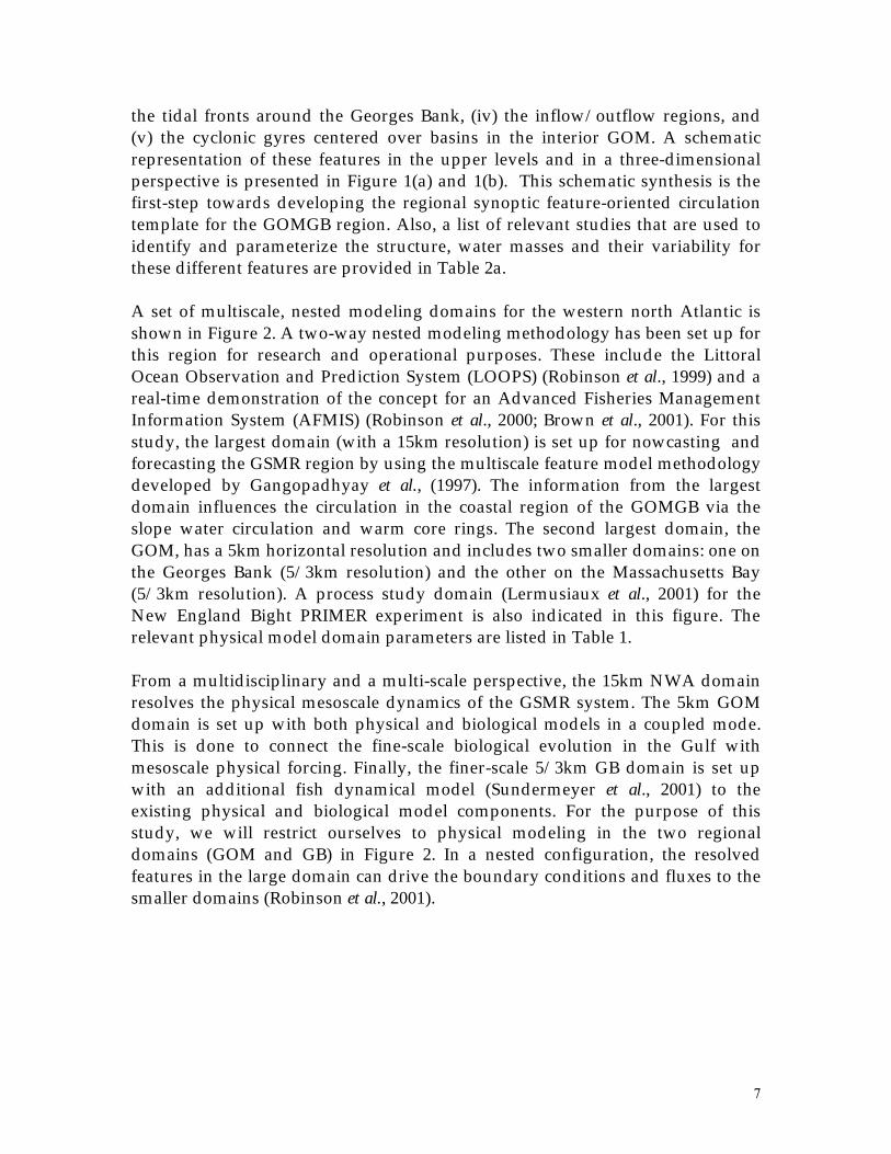
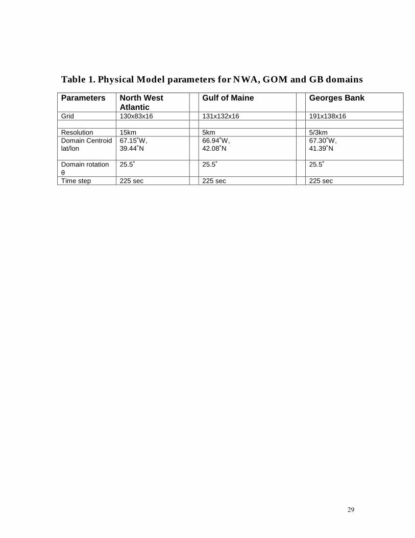
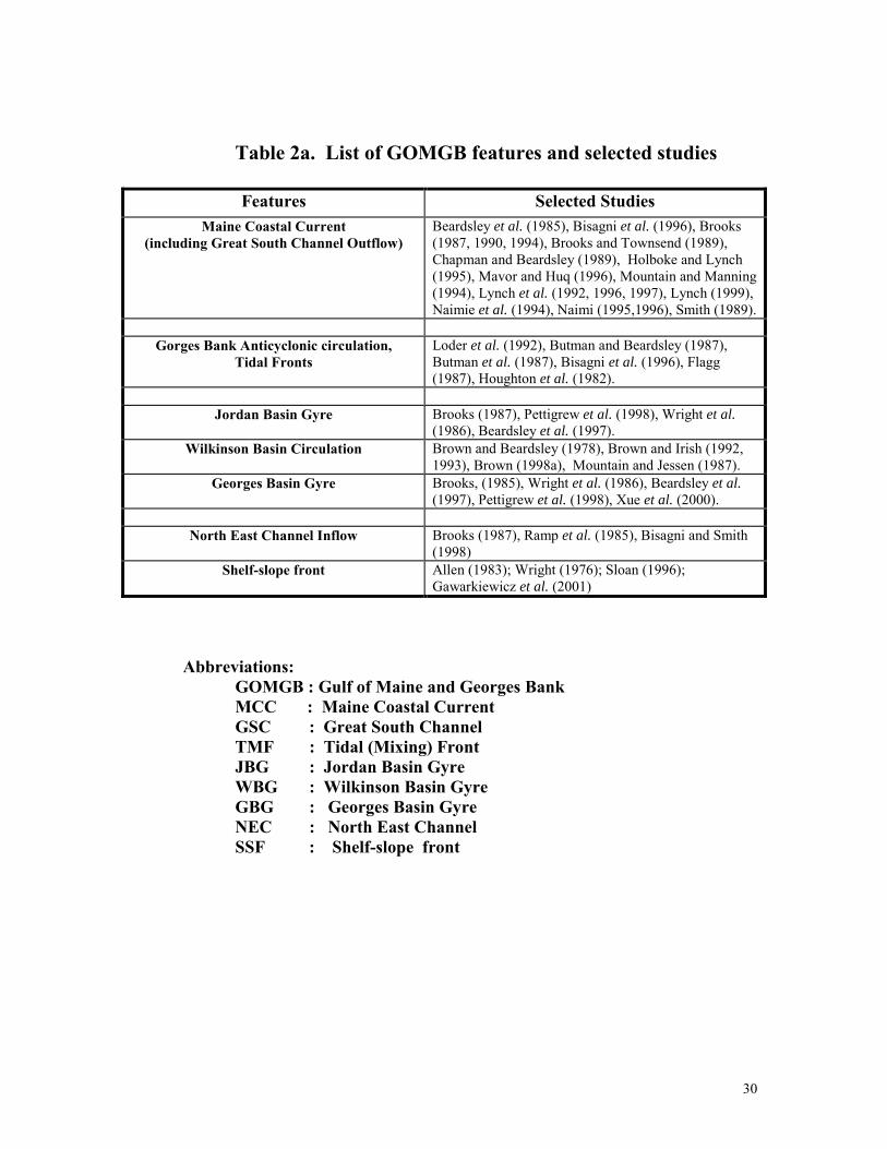
the tidal fronts around the Georges Bank, (iv) the inflow/outflow regions, and (v) the cyclonic gyres centered over basins in the interior GOM. A schematic representation of these features in the upper levels and in a three-dimensional perspective is presented in Figure 1(a) and 1(b). This schematic synthesis is the first-step towards developing the regional synoptic feature-oriented circulation template for the GOMGB region. Also, a list of relevant studies that are used to identify and parameterize the structure, water masses and their variability for these different features are provided in Table 2a. A set of multiscale, nested modeling domains for the western north Atlantic is shown in Figure 2. A two-way nested modeling methodology has been set up for this region for research and operational purposes. These include the Littoral Ocean Observation and Prediction System (LOOPS) (Robinson et al., 1999) and a real-time demonstration of the concept for an Advanced Fisheries Management Information System (AFMIS) (Robinson et al., 2000; Brown et al., 2001). For this study, the largest domain (with a 15km resolution) is set up for nowcasting and forecasting the GSMR region by using the multiscale feature model methodology developed by Gangopadhyay et al., (1997). The information from the largest domain influences the circulation in the coastal region of the GOMGB via the slope water circulation and warm core rings. The second largest domain, the GOM, has a 5km horizontal resolution and includes two smaller domains: one on the Georges Bank (5/3km resolution) and the other on the Massachusetts Bay (5/3km resolution). A process study domain (Lermusiaux et al., 2001) for the New England Bight PRIMER experiment is also indicated in this figure. The relevant physical model domain parameters are listed in Table 1. From a multidisciplinary and a multi-scale perspective, the 15km NWA domain resolves the physical mesoscale dynamics of the GSMR system. The 5km GOM domain is set up with both physical and biological models in a coupled mode. This is done to connect the fine-scale biological evolution in the Gulf with mesoscale physical forcing. Finally, the finer-scale 5/3km GB domain is set up with an additional fish dynamical model (Sundermeyer et al., 2001) to the existing physical and biological model components. For the purpose of this study, we will restrict ourselves to physical modeling in the two regional domains (GOM and GB) in Figure 2. In a nested configuration, the resolved features in the large domain can drive the boundary conditions and fluxes to the smaller domains (Robinson et al., 2001).

8

3 Temperature-Salinity Feature Models (TSFMs) Currents, fronts, eddy and gyres are individual features of the regional circulation system. For the coastal region, our choice of parameters is the individual temperature and salinity structures of these features. The feature models are thus called temperature-salinity feature models, or TSFMs. In this section, we first present a general formulation of the TSFMs, and then we describe the individual “feature models” for different features in the GOMGB region. 3.1 A general formulation The three-dimensional synoptic temperature or salinity structure for an individual feature can be described by two components. One of them is representative of its axis or core property and expressed primarily by an empirical function in the vertical. The other component describes the horizontal distribution across and along the current/front/flow feature. The following general form can be used as a simple model for a variable, ψ, which could be any tracer, velocity component, pressure, or streamfunction etc. In this study, we restrict ourselves to the tracer, i.e., the temperature or salinity structure for a current/front/flow system:

ψ (x,η,z) = ψa(x,z)+ α(x,z) Γ(η,z), 1(a) ψa(x,z) = [ψo(x) –ψb(x)] φ(x,z) + ψb(x). 1(b) Here, x is the dimensional along-stream coordinate, η is the cross-stream coordinate with its origin at the axis (center of the current), and z is the dimensional vertical coordinate (positive upward). See Figure 3 for a schematic representation of the TSFM. The core/axis profile function, ψa(x,z), is a combination of the surface (ψo(x)) and bottom (ψb(x)) values of the tracer at the axis of the feature, and φ(x,z), which is the normalized vertical tracer profile. The function φ(x,z) has a value of unity at the top (z=0) and zero at the bottom (z=H, where H is the local depth). This representation allows the choice of different set of water masses for a particular feature along-stream by varying top and bottom axis values and the structure of φ(x,z). The along-stream variations of surface and bottom temperature and salinity representation in this feature model account for the effects of river runoff, buoyancy flow input and other anomalous water masses. Similarly, the

9

along-stream variation of φ(x,z) may represent the effects of vertical mixing, branching of currents and joining of frontal systems. In the second term, the along-stream tracer amplitude variation function is represented by α(x,z), and the across-current tracer (temperature or salinity) gradient is given by Γ(η,z). In the following subsections, we will show how to simplify this term further for individual adaptation to different features. The above formulation provides a direct way to deal with local topography at a particular location. Velocities are generated subsequently through the dynamic height computation. The representative general variable ψ is representative of either temperature or salinity, as appropriate, in the following subsections. 3.2 The Maine Coastal Current (MCC)

The specific mathematical expression for the MCC TSFMs for Eq. (1):

ψM(x,η,z) = ψMa(x,z)+ αM(x,z) ΓM(η), 2(a) ψMa(x,z) = [ψMo(x) –ψMb(x)] φΜ(x,z) + ψMb(x), 2(b) and ΓM(η) = ± η 2(c) Based on observational studies (Table 2a), the three-dimensional temperature or salinity distribution for the MCC is modeled with an axis profile ψMa(x,z) and a depth-dependent cross-stream temperature or salinity gradient distribution [αM(x,z) ΓM(η)], which varies in the along-stream direction. Note that, 0≤η≤W, where W is the width of the front on either side of the axis. Melding the background climatology across the front will smooth the break in the temperature gradient by objective analysis (see Section 4). In the above expressions, a superscript in the upper case denotes linkage to a feature: M for the MCC, GB for the Georges Bank, I for the inflow and O for the Outflow. Upper case subscripts are reserved for temperature (T) and salinity (S), as the case may be. Lower case subscripts are used to identify the following: ‘a’ for axis, ‘c’ for core, ‘0’ for surface and ‘b’ for bottom. This notation will be used in general for other features, as well. Synoptic sections at different locations along the path of the MCC could ideally provide the parameters in Eq. (2) (see Table 3). However, in lieu of such synoptic information, we suggest that the characteristic temperature and salinity profiles

10

for its axis be obtained from the Department of Fisheries and Oceans (DFO), Canada database (http://www.mar.dfo-mpo.gc.ca/science/ocean/database). Example temperature and salinity profiles for the MCC near the Scotian shelf for different months are shown in Figures 4(a) and 4(b). The distinctive spread of temperature profiles in Figure 4(a) over the twelve-month period presents a formidable challenge for the development of a robust synoptic forecasting methodology that can work equally well during any such period as well as in a continuous operational mode. A feature-oriented regional modeling and simulation (FORMS) approach can have a considerable advantage over traditional methods of data initialization. However, it is important to realize the strength and power of data (however minimal it is) to calibrate and adjust the FORMS for specific nowcasts, forecasts and hindcasts. The salinity structure in Figure 4(b) for the MCC near the Scotia shelf indicates the complexity of the forecasting over a month’s interval. It is this variability that determines the horizontal and vertical gradients in the feature model design for synoptic initialization. Figure 4(c) shows the t-s variations over the twelve months, while Figure 4(d) presents a typical t-s variation along the current in the summer time. The fresh and cold Scotian Shelf water (SSW) (black curve) transits through the eastern (blue) and western (green) Gulf while becoming warm and saltier near the GSC (red). In reality, the function φΜ(x,z) (and therefore ψΜ

a(x,z)) is chosen to be empirical and depends on the season. One important aspect of φΜ(x,z) is the representation of the minimum temperature layer at mid-depth. The rationale for choosing a generalized form of φΜ(x,z) in Eq. (1) is twofold: (i) it allows for modeling the representation of the bifurcation and trifurcating as a combination of different water masses by changing the vertical structure along-stream, and (ii) it allows for the representation of effects of seasonal processes that occur in the gulf, such as vertical mixing in the winter in the western GOM; i.e., by constraining φΜ(x,z) = 1 during the wintertime, one can impose vertical mixing/homogeneity of water column for the MCC. Function φΜ(x,z) can accommodate topography variation downstream near the bifurcation region near Penobscot Bay (69˚W, 43.5˚N) and in the trifurcating region near GSC. Different segments of the MCC can be modeled by a combination of water masses through φΜ(x,z). Specifically, the upper layer (0-50m) of the eastern Maine Coastal current changes from SSW to Maine Surface Water (MSW) along the coastal Maine region. In the 50-100m-depth range, the water changes from being SSW in the eastern end to being Maine Intermediate Water (MIW) in the western Gulf region (after the bifurcation region near Penobscot Bay). In the trifurcating region near GSC, the MSW flows through the channel, the water to the west is fresher than slope water in the Nantucket Shoals

11

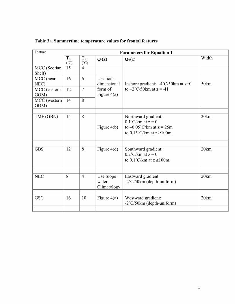
region, and the water masses to the east are more representative of the Georges Bank tidal front constituents. Such water masses can be modeled by different functional forms of φΜ(x,z). Two sections from Brooks and Townsend (1989) for two cruises in August 1987 were analyzed to infer the along- and across-stream thermal and salinity structures of the MCC. The two sections were separated by about 100km in along-stream distance. This data set, and the analysis thereof provided us with a first synoptic parameterization of the MCC in the eastern GOM during the stratified season. The temperature at the axis of the coastal current is also modeled as a function of the along-stream distance to take into account possible runoff effects and mixing with other surrounding water masses. The surface temperature (T0) was 15º C to the east and 12º C in the interior. However, the bottom temperature remained at about 8.5º C for both of these sections. Clearly, the upper 100 meters of the water column are more sensitive to the surface effects of forcing, and thus, exhibit more variability. The thermohaline slope distribution [αM(x,z)] of the current is chosen by analyzing the Brooks and Townsend (1989) data in the available sections. A spatial gradient is prescribed to model the gradual cooling trend from the offshore side of the current to the inshore side. A typical value of this gradient at the surface is about 3-4°C over a current width (η) of 50km during the stratified season. In a similar manner, the salinity profiles are represented by characteristic vertical profiles, non-dimensional horizontal spatial gradients for gradual freshening of water masses, and a surface salinity amplitude value. Selected parameter values following Eq. (1) for temperature and salinity profiles during a typical month of June are listed in Tables 3(a) and 3(b), respectively. Parameter choices for other months will need to be adjusted within the observed ranges of variation for such profiles. Seasonal bounds for the surface parameter values for the MCC and other features are listed in Table 3(c). 3.3 The Shelf-Slope Front (SSF) The shelf-slope front (SSF) is a transition between the cold, fresh shelf water and warm, saltier Slope water extending from Cape Hatteras (north of the Gulf Stream) through Mid Atlantic Bight and beyond the NEC. The surface signature of the SSF is one of the most readily observable features from satellites (Halliwell and Moores, 1979). Wright (1976) analyzed the interaction of the front with bottom topography and determined that 80% of the time, the front remained within 16km of the 100m isobath. The SSF is primarily density dependent (Allen

12

et al., 1983; Sloan, 1996; Gawarkiewicz et al. 2001), with salinity dominating the density constituents. A temperature-salinity feature model originally developed by Sloan (1996) and used for assimilation studies in coastal region (Robinson et al., 1998; Lermusiaux et al., 2001), is adapted here. The SSF is modeled as a melding region of two water masses (shelf and slope) along and across the shelf-break region. The elements of the SSF include the following: defining the mean location at the surface from satellite observations and defining the isotherm and isohaline corresponding to the mean location at the bottom (Wright, 1976; Mountain, 1991), the thermocline slope (Chapman and Gawarkiewicz (1993); Houghton et al., 1988, 1994), the width (Behrens and Flagg, 1986) and the melding function. Linder and Gawarkiewicz (1998) provide a comprehensive description of the climatology of the shelf-break front from the southern flank of the Georges Bank, through the region south of Nantucket Shoals and off the coast of New Jersey. Specifically, the shelf-slope front tracer (temperature or salinity) distribution is modeled by: ψss(x,y,Z) = ψsh (x,z) + (ψsl (x,z) – ψsh(x,z)) µ(η,Z), (3a) where µ is the melding function:

µ(η,Z) = ½ + ½ tanh[(η-θ·Z)/γ]. (3b) Here, θ is the slope (tilt), Z is the depth, γ is the e-folding half-width of the front, and η is the cross-frontal distance. In terms of the general formulation (Eq. 1), the core is given by the shelf structure. The horizontal distribution of the SSF is represented by the melding function. The tracer amplitude function, α(x,z), is given by the difference between the slope and the shelf structure. For a schematic representation of this implementation, see the study by GR02. A typical implementation of SSF includes choosing a value of θ between 0.001 and 0.008 and setting γ equal to 15km. The melding is performed between 100m in shallow regions to 300 meters in the deep end. 3.4 Fronts around Georges Bank During the winter season, the flow over the Georges Bank consists primarily of tidal rectification due to tides interacting with the steep topography. In the summer and fall, stratification sets in with an increasing flow due to the

13

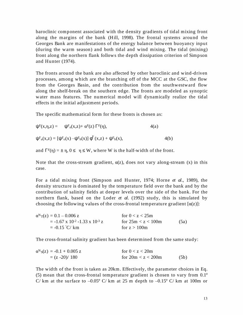
baroclinic component associated with the density gradients of tidal mixing front along the margins of the bank (Hill, 1998). The frontal systems around the Georges Bank are manifestations of the energy balance between buoyancy input (during the warm season) and both tidal and wind mixing. The tidal (mixing) front along the northern flank follows the depth dissipation criterion of Simpson and Hunter (1974). The fronts around the bank are also affected by other baroclinic and wind-driven processes, among which are the branching off of the MCC at the GSC, the flow from the Georges Basin, and the contribution from the southwestward flow along the shelf-break on the southern edge. The fronts are modeled as synoptic water mass features. The numerical model will dynamically realize the tidal effects in the initial adjustment periods. The specific mathematical form for these fronts is chosen as: ψF(x,η,z) = ψFa(x,z)+ αF(z) ΓF(η), 4(a) ψFa(x,z) = [ψFo(x) –ψFb(x)] φF (x,z) + ψFb(x), 4(b) and ΓF(η) = ± η, 0 ≤ η ≤ W, where W is the half-width of the front. Note that the cross-stream gradient, α(z), does not vary along-stream (x) in this case. For a tidal mixing front (Simpson and Hunter, 1974; Horne et al., 1989), the density structure is dominated by the temperature field over the bank and by the contribution of salinity fields at deeper levels over the side of the bank. For the northern flank, based on the Loder et al. (1992) study, this is simulated by choosing the following values of the cross-frontal temperature gradient [α(z)]: αNT(z) = 0.1 – 0.006 z for 0 < z < 25m = -1.67 x 10-2 -1.33 x 10-3 z for 25m < z < 100m (5a) = -0.15 ◦C/km for z > 100m The cross-frontal salinity gradient has been determined from the same study: αNS(z) = -0.1 + 0.005 z for 0 < z < 20m = (z -20)/180 for 20m < z < 200m (5b) The width of the front is taken as 20km. Effectively, the parameter choices in Eq. (5) mean that the cross-frontal temperature gradient is chosen to vary from 0.1º C/km at the surface to –0.05º C/km at 25 m depth to –0.15º C/km at 100m or

14

deeper. The cross-frontal salinity gradient in the surface is chosen as –0.10 ppt/km, which increases to zero at 20m, and to 1ppt/km at depths of 200m over the side of the Bank. The vertical profiles of temperature and salinity at the axis of the front are chosen from the DFO climatology and are shown in Figures 5(a) and 5(b). The monthly variability in the t-s space for the northern flank of the Georges Bank is shown in Figure 6(a). For the front on the southern flank of the Georges Bank, the following values of the cross-frontal temperature gradient are chosen (Flagg, 1987): αST(z) = 0.2 – 0.001 z for 0 < z < 100m = -0.1 ◦C/km for z ≥ 100m (6a) The cross-frontal salinity gradient has been similarly obtained as: αSS(z) = 0.15 - 0.0005 z for 0 < z < 100m = 0.10 ppt/km for z ≥ 100m (6b) The vertical profiles of temperature and salinity at the axis of the front are chosen from the DFO climatology and shown in Figures 5(c) and 5(d). The monthly variability in the t-s space is also shown in Figure 6(b). The water mass on the central region of the Georges Bank, where the bank is shallower than 60m, is stratified during the summer months and well mixed during winter. This is given by: ψGB(x,η,z) = ψGB(z). (7) The simplest adaptation of the general formulation for the TSFM is obtained for the Georges Bank well-mixed region, when ψGB(z) = ψmixed, and ψmixed is a single value. The temperature and salinity structures for this water mass in different months can be obtained from a single synoptic observational profile or taken from the DFO database. The climatological variability in the t-s space for this water mass is shown in Figure 7(a). 3.5 Channel Inflow and Outflow The mathematical form for the TSFMs for the inflow through the NEC or the outflow through the GSC can be given by the following adaptation of Eq. (1): ψI(x,η,z) = ψIa(x,z)+ αI ΓI(η), 8(a)

15

ψIa(x,z) = [ψIo–ψIb] φI(x,z) + ψIb(x), 8(b) and ΓI(η) = ± η, 0 ≤ η ≤ W, where W is the half-width of the front. The temperature feature-model for the inflow is based on the Ramp et al. (1985) study. Its vertical structure, φI(x,z), is taken as the Slope water climatology profile. The salinity structure is adapted as φI(x,z) = (1 - z/H), where H is the depth of the NEC. Furthermore, the depth-independent cross-frontal eastward temperature and salinity gradients values are adapted for αIT = -0.04 ◦C/km and αIS = -0.1 ppt/km. For the outflow, the temperature structure is also based on the Ramp et al. (1985) study. In this case, φO(x,z), is determined from the DFO database. Similar to the inflow, the salinity structure is adapted as φO(x,z) = (1 - z/H), where H is the depth of the GSC. The depth-independent cross-frontal westward temperature and salinity gradients values are determined as αOT = -0.04 ◦C/km and αOS = -0.05 ppt/km. See Tables 3(a) and 3(b) for selected temperature and salinity parameter values for the month of June and Table 3(c) for seasonal variations for the surface temperature (T0). 3.6 The Cyclonic Gyres in the interior Gulf The interior GOM has cyclonic circulation regions situated over three deep basins – Georges, Jordan and Wilkinson. The gyres are set up by the deep inflow of saline waters through the NEC and forced by topography (Hannah et al., 1996; Lynch, 1999). It has been observed that the dominant temporal variability in the gyres or between gyres is on the order of months (Xue et al., 2000). The temperature and salinity distribution of these sub-basin scale gyres can be modeled by assuming a core profile and a decay or growth function along the radial direction to the surrounding water masses. Conforming to Eq. (1), the following functional form can be adopted as a simple gyre feature model: ψ (r,z) = ψc (z) - [ψc (z) - ψk (z) ] {1-exp(-r/R)}. (9a) Here, r is the radial distance from the center of the gyre, z is the depth, Tk(z) is the background and Tc(z) is the core tracer (temperature or salinity) profile. Typically, R= 5 R0, where R0 is the Rossby radius. Rearranging the terms in the above equation, we get:

16

ψ (r,z) = ψc (z) exp(-r/R) + ψk (z) {1 – exp(-r/R)}. (9b) These two terms represent two different contributions. The core profile ψc(z) exponentially “fades out” to the background distribution ψk(z). Also, the latter exponentially “fades in” to replace the core signature as ‘r’ increases away from the center of the feature. Synoptic observational studies are used to extract feature-model water-mass structures (ψk(z) and ψc(z)) for these different gyres. Figure 9 shows examples of some available sections from Brooks (1990) and Pettigrew et al. (1998) studies in the GOMGB region. As a first approximation, the interior gyres are feature- modeled as distinct water masses over the three basins. Climatological variations of the water mass properties of these three gyres in the GOM are shown in Figures 7(b), (c), and (d) for the Georges, Wilkinson and Jordan basins. The monthly variations in their temperature and salinity profiles as obtained from the DFO database are presented in Figure 8(a) through Figure 8(f). As will be shown later, the ensuing dynamical model simulation generates reasonable cyclonic flows around the basins within a few time-steps of integration, so that the synoptic interaction between the currents/fronts and gyres can occur.

3.6.1 The Jordan and Georges Basin Gyres These two gyres are located in the eastern Gulf with a north-south orientation. Each has an inner core in almost solid-body rotation, constrained by the topographic Taylor column (Cushman-Roisin, 1994). Thus, the core and background profiles in Eq. 9(b) for each of these basins are set to a single profile. These choices are listed in Table 4 and explained below. The core of the Georges basin gyre has a larger radius (20km). Its center is located at 42.42 N/ 67.17W. The representative temperature and salinity profiles are derived from section S (S11-S17) of the Pettigrew et al. (1998) study for the summer simulations (see Figure 9). In addition, the core vertical profiles of temperature and salinity for the winter-spring period were chosen from the DFO climatology. These are shown in Figures 8(b) and 8(e). The variability in the t-s space is also shown in Figure 7(c). The setup of the Jordan basin gyre is very similar to that of the Georges basin gyre. The core of the Jordan basin is taken as one with a radius of 15km with its center located at 43.627N/67.775W (Station S11 in Pettigrew et al., 1998). For the purpose of this study, the Pettigrew et al. (1998) observations (F4-F20, and S8-S11) were used for summer simulations, as described in Section 5. The vertical profiles of temperature and salinity at the core were chosen from the DFO

17

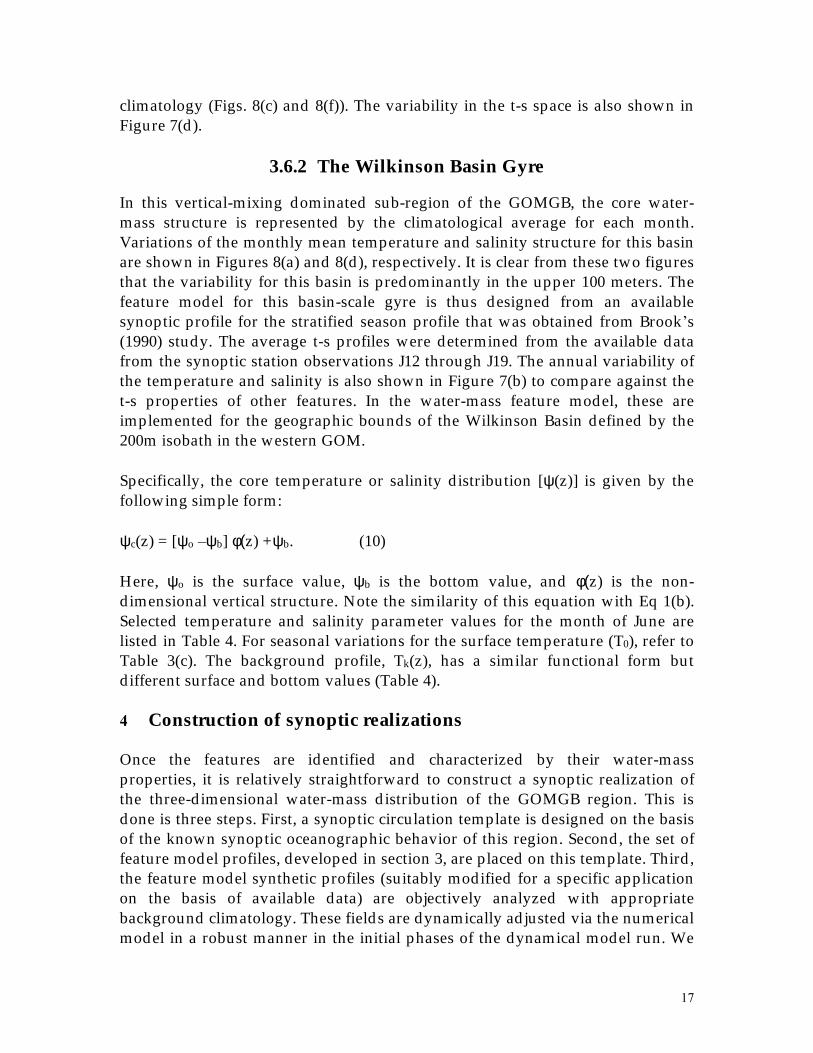
climatology (Figs. 8(c) and 8(f)). The variability in the t-s space is also shown in Figure 7(d).

3.6.2 The Wilkinson Basin Gyre

In this vertical-mixing dominated sub-region of the GOMGB, the core water-mass structure is represented by the climatological average for each month. Variations of the monthly mean temperature and salinity structure for this basin are shown in Figures 8(a) and 8(d), respectively. It is clear from these two figures that the variability for this basin is predominantly in the upper 100 meters. The feature model for this basin-scale gyre is thus designed from an available synoptic profile for the stratified season profile that was obtained from Brook’s (1990) study. The average t-s profiles were determined from the available data from the synoptic station observations J12 through J19. The annual variability of the temperature and salinity is also shown in Figure 7(b) to compare against the t-s properties of other features. In the water-mass feature model, these are implemented for the geographic bounds of the Wilkinson Basin defined by the 200m isobath in the western GOM. Specifically, the core temperature or salinity distribution [ψ(z)] is given by the following simple form: ψc(z) = [ψo –ψb] φ(z) +ψb. (10) Here, ψo is the surface value, ψb is the bottom value, and φ(z) is the non-dimensional vertical structure. Note the similarity of this equation with Eq 1(b). Selected temperature and salinity parameter values for the month of June are listed in Table 4. For seasonal variations for the surface temperature (T0), refer to Table 3(c). The background profile, Tk(z), has a similar functional form but different surface and bottom values (Table 4). 4 Construction of synoptic realizations Once the features are identified and characterized by their water-mass properties, it is relatively straightforward to construct a synoptic realization of the three-dimensional water-mass distribution of the GOMGB region. This is done is three steps. First, a synoptic circulation template is designed on the basis of the known synoptic oceanographic behavior of this region. Second, the set of feature model profiles, developed in section 3, are placed on this template. Third, the feature model synthetic profiles (suitably modified for a specific application on the basis of available data) are objectively analyzed with appropriate background climatology. These fields are dynamically adjusted via the numerical model in a robust manner in the initial phases of the dynamical model run. We

18

first describe the construction of a typical synoptic realization in this section, and we then present a set of example dynamical model simulations and sensitivity studies in the next section. 4.1 Development of a synoptic feature-oriented circulation template Initialization of any dynamical model requires the specification of each prognostic variable at each grid point of the three-dimensional model domain. A typical mesoscale resolution domain in the GOMGB region (GOM in Figure 2) consists of 131x132 grid points in the horizontal with 5km resolution (Robinson et al., 1998). Sixteen vertical levels were chosen for both GOM and GB domains in this coastal region, with a terrain-following coordinate system (Haley and Lozano, 1999). Thus, it would require around 5x105 degrees of freedom for each prognostic variable to describe a synoptic state of this coastal system. To quantify the information needed to represent a feature-oriented regional modeling system, consider setting up a synoptic realization. As described in Section 3, the feature models are represented in terms of their temperature and salinity structures and a few parameters listed in Tables 3 and 4. First, the location of each of these features is identified from various data sources, such as broad-scale National Marine Fisheries Services (NMFS) surveys, coastal moorings, buoy information, synoptic surveys and satellite imagery, which include AVHRR, Color and Altimeter (if possible to use). The feature models can then be placed in the analysis domain in their various representations. For example, the MCC can be represented by three major segments, two with bifurcating regions near the Bay of Fundy and near Penobscot Bay, and one with a trifurcating region near the GSC. The Georges Bank frontal system follows the topography very well, which presents an advantage in locating these features. The strengths of the three sub-basin scale gyres and the identification of anomalous features are the critical unknowns in this feature-model approach. Identifying frontal features from satellite imagery for surface temperature and color is sometimes challenging in coastal regions due to cloud coverage and due to loss of signal as a result of interaction with land for altimetric signals. It is thus important to develop a scheme for specifying ‘default’ locations of coastal features in lieu of satellite observations. We rely on dynamical considerations to develop such a scheme. Coastally important flows are typically constrained by topography in a potential vorticity sense. Furthermore, initial bathymetric layout of features can be dynamically adjusted by interactions with tides, winds, and heat and buoyancy fluxes in the ensuing numerical model integration. For example, the MCC is generally observed to be flowing within the 100m isobaths. Considering the half-width of the current as 50km, we recommend

19

using the 50m isobaths as the ‘default’ axis location of the MCC when satellite observations are not available. Next, following the dynamical reasoning of Simpson and Hunter (1974), the ‘default’ axis of the tidal mixing front is placed at the 50m topographic contours between 69˚W and 66˚W along the northern flank of the Georges Bank. Similarly, the southern front’s axis is taken as the 60m isobaths around the southern flank between 71.6˚W and 66˚W. In the present implementation of feature-oriented initialization, a set of strategic locations are chosen across and along the fronts based on prior knowledge of the frontal behavior, model resolution and intended dynamical process study. For synoptic forecast system implementation, one needs to resolve evolving meanders, cross-frontal exchanges, eddy-frontal interactions, etc. For MCC, considerations must be given to (1) resolving bifurcations and trifurcations, (2) resolving interactions with Jordan and Wilkinson gyres and (3) balancing the inflow through Scotian Shelf and outflow through the GSC. In terms of TMF around the northern flank, high-resolution sampling at 5/3km across the front was proved to be essential. This will be discussed later in Section 5. A set of strategic locations based on above dynamical considerations for all the features is called the `synoptic circulation template’ for the region. The template for the GOMGB is shown in Figure 10. In addition to the MCC, the TMF, the SSF front and the inflow/outflow system, the topographically controlled gyres are strategically sampled for initialization as well. The gyres’ mean locations and geographical extents are preset from observational studies as default, and listed in Table 4. The eddy, or gyre structures are best resolved with a cross-hair sampling as shown in Figure 10. The major advantage in using such a template is the ability to resolve synoptic structures on the basis of past oceanographic knowledge of the region, even when there is a lack of observations for the synoptic features. Note that only a handful (270 for GOMGB) of stations are needed to describe the synoptic behavior of this regional ocean. The ‘default’ template should be used as a guide to place the synoptic feature model profiles, and can be adjusted according to available satellite or in situ observations for a specific nowcasting, forecasting, hindcasting or updating exercise. 4.2 Feature-oriented initialization for the shelf-slope coastal ocean A six-step procedure is followed to generate the three-dimensional initialization fields for modeling in the GOM or GB domains. These are (i) placing the individual synoptic TSFMs in a collective feature-oriented circulation template; (ii) creating shelf objective analysis, or, OA t-s fields; (iii) creating the deep OA fields; (iv) melding the shelf and slope t-s OA fields through the shelf-slope front; (v) adjusting the shelf and slope dynamic height OA fields to bottom

20

topography; and (vi) generating the equivalent barotropic streamfunction for the numerical dynamical model. First, the temperature and salinity feature-model fields are selectively sampled along and across the important features, as shown in Figure 10. The red dots in Figure 10 are the locations chosen for sampling the five important features of circulation for this region. This strategic feature-oriented arrangement (feature model profiles in the template locations) ensures the presence of synoptic structures in the initialization and updating fields for nowcasting and forecasting. Temperature and salinity profiles for the individual TSFMs are obtained using the equations in Section 3 and placed at their appropriate locations in Figure 10. Second, this collection of temperature and salinity profiles are treated as pseudo-CTD observations and objectively analyzed (Carter and Robinson, 1987; Watts et al., 1989; Lermusiaux, 1999a) with appropriate background seasonal climatology in the coastal shelf domain. Figure 11(a) shows the location of climatological profiles derived from MARMAP (Marine Resources, Monitoring, Assessment and Prediction Program) and NMFS (National Marine Fisheries Services) data sets, which is used as the background climatology. The resolution of the climatology is ¼ degree (25km), which is inadequate to represent the mesoscale variability of this region with prevalent length scale (Rossby radius) on the order of 5-10km. The resulting shelf OA field for temperature and salinity thus combines the synoptic structures in a background of available climatology, appropriate for nowcasting and forecasting. A typical climatology from GDEM (Teague et al., 1994) has a coarse resolution of 1˚ (Fig. 11(b)). A high-resolution climatology at 8km was developed later as part of the AFMIS operational program. The methodology will be reported by Brown et al. (2002). The OA is performed in two stages (Lermusiaux, 1999a). In the first stage, the largest dynamical scales are resolved at each level, using estimated large-scale e-folding spatial decays, zero crossings, and temporal decay. The background field for this first stage is the horizontal average of the climatology data. In the second stage, the synoptic dynamics of interest (meso-scale and sub-basin scale) are resolved using its estimated space-time decays. The background for this second stage OA is the first-stage OA. The primary assumption made in this two-scale OA is that the errors in the climatology (first-stage) and synoptic (second-stage) dynamical scales are statistically independent. This procedure effectively and smoothly melds the synoptic feature model or observational profiles and climatology for the shelf region. The OA parameters (space-time decay scales, zero crossings) used for climatology and feature-model profiles for the GOM and GB domains are listed in Table 3. For detail mathematical description of the OA parameters, see Lermusiaux (1999a,b).

21

The uncertainties in the feature model profile values can also be obtained from the DFO database. The monthly climatological standard deviations provided in this database are adapted as estimates of error for the axis profiles, as applicable (see Table 3-4 and Figs. 4-8). These estimates are however conservative, and any available data (including satellite and buoy observations) should be used to readjust these OA parameters on a case-by-case basis. As mentioned earlier, the coastal regions of the GOMGB contain the continental slope region, and affected by the slope water circulation and warm core rings from the GSMR deep-water region. It is thus necessary to meld the shelf OA fields of temperature and salinity with those from the synoptic GSMR feature model fields from Gangopadhyay et al. (1997). Starting from available satellite and in situ observations for a particular day, the GSMR methodology provides a kinematically consistent set of temperature, salinity and velocity fields in the 15km NWA domain. These initial (deep) fields are first mapped and then interpolated on the finer-scale (5-km) coastal GOM grid points. The deep and the shallow fields (t-s) are then blended along and across the shelf slope front using Eq. (3) in Section 3.3. An important consideration of melding the shallow and deep fields is the lack of geostrophic compatibility between the melded t-s and dynamic height fields between the shallow (shoreward of SSF) and the deep (slopeward of SSF) sub-regions within the modeling domains of the GOM and the GB. This is due to the fact that the levels of no motion used to compute the dynamic height from the temperature-salinity fields are generally different for the two sub-regions. This incompatibility is addressed in four steps: (i) by computing surface velocity (u, v) in both shelf and deep domains using geostrophy; (ii) melding the surface (u,v) fields; (iii) solving the Poisson equation to get surface dynamic height; and (iv) finally integrating the density anomaly derived from the melded t-s fields from surface down to get the subsurface dynamic height. In the end, after the melding of the two topographically adjusted fields, a barotropic transport component is added to the baroclinic velocity (derived from the t-s fields) to complete the Initialization. This barotropic transport component is generally specified via streamfunction (see Gangopadhyay et al., 1997 for details), which may be obtained in two ways. It may be specified a priori, i.e. from estimates of previous studies such as Brown (1998b) for a particular season, or derived from available current meter or ADCP data. However, lack of in situ data and matching synoptic information in real-time oceanographic forecast exercises is quite common. A default transport streamfuntion is then estimated based on vertical averaging of the melded velocity components.

22

The deep-to-shelf melded and topographically adjusted three-dimensional dynamic height field (from step (iv) above) is differentiated to produce horizontal velocity field on flat levels. The horizontal velocity is interpolated to terrain-following (σ) levels. The interpolated velocity field is integrated in the vertical to produce the first-guess barotropic velocity (u,v). The barotropic vorticity is then obtained from a curl of the first-guess barotropic velocity (ξ=∂v/∂x - ∂u/∂y). Dirichlet boundary conditions for the transport streamfunction are obtained by integrating the normal component of the barotropic velocity through the boundary. A correction factor based on this velocity is applied to ensure zero net transport through the boundaries. The default transport streamfunction (ψ) is then constructed by solving a Poisson equation forced by the barotropic vorticity (ξ) with these boundary conditions (∇ 2ψ=ξ). This depth-averaged first-guess transport streamfunction is used in the initialization, which evolves and adjusts to the non-linear dynamics of the primitive equations in the ensuing integration. Such field adjustment was achieved in the GSMR region (Robinson and Gangopadhyay, 1997) in a period of 1-3 days. For the GOM and GB regional domains, such adjustments seem to take place within the first one or two tidal periods, as experienced in the early simulation during AFMIS real-time exercises (Robinson et al., 1999). 5 Dynamical Simulations In order to calibrate the parameters of the feature models for realistic behavior in the regional domains, a series of sensitivity studies will be necessary. Such simulations will include the effects of tides, winds, and buoyancy flow to understand the important scale and modes of dominant variability that occur in this complex coastal region. Here, we present three simulations – two in the GOM domain and one in the GB domain. The first simulation in the GOM is a 10-day long forecast without any external forcing. Next, a high-resolution 10-day long simulation is presented in the GB domain. The final simulation is a short-term (3-day long) case study in the GOM with successive application of winds, heat flux and evaporation/precipitation fields. 5.1 Model Computational Parameters A real-time forecasting experiment was carried out during March-April 2000 using the Harvard Ocean Prediction System (HOPS) for the GOMGB region. The

23

dynamical model is the non-linear primitive equation (PE) model of HOPS (e.g. Robinson, 1996), in its rigid-lid configuration. The values for the physical parameters for the two domains (GOM and GB) are listed in Table 1. The values for the calibrated numerical parameters are listed in Table 6. For both model domains, 16 vertical levels are distributed based on a “double sigma” transformation (Lozano et al., 1994; Sloan, 1996). This is a piecewise linear transformation, which uses two “terrain-following” sigma systems: one from the surface to an intermediate depth hc(x,y), the other from hc to the bottom. For suitably chosen hc, this maintains relatively flat levels above hc in both the shallow and deep oceans for the two domains. The time step for both model runs was chosen as 225 seconds. Horizontally, the parameterization of the subgrid-scale mixing processes and filtering of numerical noise is based on a Shapiro filter (Shapiro, 1970). Its parameters are: order (p), number of applications per time step (q), and frequency of application (every r time-steps). For each state variable (u, v, t, s, streamfunction and vorticity), the values of p, q and r were selected based on curves of effective diffusivity as a function of horizontal scales, and a compromise between smoothing computational noise and allowing physical instabilities (Lermusiaux, 1999b). The vertical mixing is Lapacian, with fixed eddy viscosity Av = 0.5 cm2s-1 for both domains. The eddy diffusivity (Kv) was kept small (0.05 cm2s-1 ) for both the smaller domains to allow for tidal mixing compared to the original mesoscale value of 0.5 cm2s-1 for NWA. Convective adjustment is applied when the water column is statically unstable, with a vertical viscosity Avcvct and a vertical diffusivity (Kvcvct), both of which have the same value of 50 cm2s-1 for the GOM and 10 cm2s-1 for the GB domains. At the open boundaries, Orlanski radiation (ORI/ORE) conditions (Orlanski, 1976) were preferred for all variables. Across coastlines, the normal flow and tracer flux are set to null values. Along coastal boundaries in the GOM domain, the tangential flow is subjected to a Rayleigh friction of relaxation time Tc = 1800s and Gaussian decay horizontal-scale of 2 grid points, Lc = 10km. This condition is a “damped free-slip.” At the bottom, a dynamic stress balance is applied to the momentum equations, with a drag coefficient Cd = 2.5 x 10-3. Any assimilation application will require error estimates for the feature-oriented initialization fields. The two-stage OA described in Section 4 generates such error fields while melding the synoptic feature-model profiles with background climatology. Strategic sampling of features, as described in Section 4.2 and Figure 10, helps assign observational error or confidence in feature model profiles and available data in an objective manner. For example, while using SST imagery to detect frontal regions, high confidence (less observational error) can be placed for feature-model profiles placed strategically through gaps in a cloudy image. Such assimilative usage of feature-oriented modeling can be performed with the

24

HOPS assimilation methodologies described by Lozano et al. (1996). In the following three subsections, we present example simulations using the feature-oriented approach in a forecast mode, without assimilation. 5.2 Simulations in the GOMGB without atmospheric forcing

We first present a 10-day long simulation in the GOM during April, 2000. Satellite observations (SST) in the NWA and the GOM were analyzed to locate the features (GS, Rings, coastal currents and gyres) and their geographical extents. Supplemented by ‘default’ feature-model profiles and other available in situ observations, synoptic initialization fields in the GOM are developed as described in Section 4.1. The six-step procedure described in Section 4.2 was then followed to derive the initial fields of temperature, salinity and velocity distribution for the GOM domain. These initial fields are then used for dynamical forecasting by the primitive equation model in HOPS. The simulation model parameters for different domains are outlined in Section 5.1. Figures 12(a) and (b) show the initial fields of temperature and salinity for April 9, 2000. The nearly uniform observed surface temperature field in the GOM was complemented by a salinity structure from feature-model methodology. This resulted in a reasonable flow along the coast (MCC), a Jordan basin cyclonic gyre flow, a weak Wilkinson basin cyclone, as well as an anticyclonic frontal system around Georges Bank. These flow fields are clear in the superimposed velocity vectors in Figures 12(a) and (b). The temperature and salinity fields at a depth of 10m (level 3) show similar flow patterns in Figures 12(c) and (d). Note that the relatively colder patch south of the SSF in the slope was an effect of fusion of SST at the initialization in the GSMR temperature fields. The 10-day forecast fields for days 1, 4, 7 and 10 are shown in Figure 13. The structure and flow fields on certain segments along the MCC and in the Jordan basin gyre are reasonable during the 10-day simulation. The coastal current is continuous during the initial three days of the simulation but changes direction or diffuses in patches later on. No atmospheric forcing was applied to these simulations. The MCC appears to be reversing off the tip of Nova Scotia, which might be due to lack of appropriate boundary conditions at the inflow. Two other aspects of this simulation were the following: (i) large-amplitude meandering of the shelf-slope front affects the flow in the eastern half of the GOM domain; (ii) detoriation of the integrity of the northern flank jet around Georges Bank occurred. While the first issue may be related to design of a better melding methodology and boundary conditions, the evolution and maintenance of tidal fronts around the Bank might be related to the underlying resolution of the dynamical model simulation. The horizontal resolution of the GOM domain

25

is only 5km, which provides only three (or, even two) cross-front grid points to resolve the gradient (and topography, as well) on the northern edge of the Bank. For the second simulation, the initial conditions are now generated from the same combination of coastal feature models and deep-water profiles (from GSMR feature models). However, the objective analysis and subsequent deep-shallow melding are performed at a higher resolution (5/3km). The strategic feature-oriented sampling of feature-model profiles are first done at a higher resolution (see Figure 10) to better resolve the cross-frontal structure around Georges Bank. The initial temperature OA fields (with superimposed velocity vectors) are presented in Figure 14(a). Note the robust realization of the anticyclonic gyre on top of Georges Bank in contrast to the coarse resolution realization shown earlier in Figure 12(b). Also note the signature of the trifurcating of the flow near the northwest corner of the GB domain, which is the outflow region (GSC) of the GOMGB circulation system. The flow fields are also reasonable south of the Bank and at deeper levels (not shown). This simulation was carried out for 10 days, without atmospheric winds, from April 9 through April 18, 2000. The resulting fields on days 3, 6 and 9 are shown in Figures 14 (b), (c) and (d), respectively. There are two major improvements in this simulation compared to the one presented for the GOM domain in Figure 13. The circulation around the Bank is more robust in this finer resolution run and the integrity of the shelf-slope front is better maintained throughout this simulation. The temperature field is maintained and velocity flow fields are within reason for up to 10 days, shown in Figure 14 (a), (b), (c) and (d) for days 0, 3, 6 and 9, respectively. Another example forecast from the GR02 study in the GB domain is briefly mentioned here in passing. A 10-day long simulation during June 6-16, 2000 was carried out with tidal mixing. The mesoscale activity along the shelf-break generates realistic shingles and plumes interacting with the southern edge of the Georges Bank. The anticyclonic circulation around Georges Bank was well maintained through day 7, after which the western boundary region was affected by an advection of a temperature plume through the GSC. The integrity of the tidal (mixing) front was maintained through the 10-day simulation, which showed that the combination of tidal mixing and baroclinic effects was reasonably simulated by this set of parameterizations in the numerical model. 5.3 Simulations in the GOM with atmospheric forcing Next, we present a short-term 3-day simulation during 25-28 June 2001, to illustrate the stability and robustness of the FORMS methodology with wind forcing, heat flux and evaporation-precipitation (E-P) fields. Figures 15(a) and

26

15(b) show the temperature (background color) and velocity field (superimposed arrows) of the operational forecast for model days 1 and 3 without any forcing. This simulation was successively forced with daily winds, heat flux and E-P fields based on available FNMOC operational nowcast and forecast products. The computed wind stress, heat flux and E-P for model day 1 are shown in Figure 16 (a), (b) and (c) respectively. A set of forecast temperature and velocity difference fields are presented in Figure 17 to show the impact of wind stress, heat flux and E-P on the GOMGB circulation modeling via FORMS. All of the difference fields are for model day 3. Figure 17(a) shows the difference between the forecasts with wind-forcing and those without wind-forcing. The wind effects are more visible in the shallow Scotian Shelf and Nantucket Shoals region, as well as the eastern Gulf and along the coastal Maine, where mixing cools the upper ocean. Also visible is mesoscale and sub-mesoscale wind-induced advection (and probably mixing) in patches along the southern and northern flanks of Georges Bank. An apparent general cooling along the SSF is observed in the model simulation. This happens due to an offshore translation of the SSF caused by southeastward Ekman flow generated by northeastward winds during days 1-3 (see Figs. 17(a) and (d)). The difference between the simulation with both wind and heat flux to the no-forcing simulation is presented in Figure 17(b). It is clear from this graphic that the impact of heat flux and wind stress is cumulative as well as complimentary in different regions of the GOM. In order to better understand the relative impact of wind and heat forcing, the difference between the ‘wind- and heat-forced’ simulation and the `wind-forced’ simulation is presented in Figure 17(c). The impact of heat flux is clearly seen as a uniform warming of the interior Gulf, around Georges Bank and the slope water region. The meoscale and sub-mesoscale advective and mixing effects of wind stress, combined with the uniform warming effect of heat flux, creates the multiscale dynamic environment of the GOM region, which is well-illustrated by this set of simulations. Finally, the impact of E-P for this period is presented in the ‘salinity difference’ field (Figure 17(d)) from the ‘wind- and heat- and E-P-forced’ simulation to the ‘wind- and heat-forced’ simulation. It is evident that in this particular case, the impact after 3 days is limited to coastal regions within the Gulf, except for the freshening of a patch (due to precipitation) in the eastern side of the domain in outer Scotia Shelf.

27

6 Summary and Conclusion We have presented a feature-oriented regional modeling and simulation (FORMS) methodology for the GOMGB multi-scale coastal circulation system. In doing so, a set of important features and their characteristic water masses have been identified and parameterized. The features include the buoyancy-driven Maine Coastal Current (MCC), the shelf-slope front (SSF), the Georges Bank anticyclonic frontal circulation system including the tidal mixing front (TMF), the basin scale cyclonic gyres (Jordan, Georges and Wilkinson), the deep inflow through the NEC, and the shallow outflow via the GSC. The individual feature models are cast in a hydrographic framework and called temperature-salinity feature models, or TSFMs. The adapted general expression for a TSFM for any front, eddy or gyre has two components. The first describes its central core or axis profile; the second represents the horizontal distribution of its water mass properties. All of the seven coastal features in this region (MCC, SSF, TMF, southern flank front, inflow/outflow and the basin-scale gyres) are described individually as a derivative of this general form. The individual mathematical expression for each feature was chosen on the basis of its dynamical behavior based on past observational studies. The simplest of these is the single-profile description of the Georges Bank gyre water mass, while the most challenging was the expression of different segments of the MCC, by appropriate along-stream structure variation. Using observational synoptic studies listed in Table 2a, a central set of parameter values for the synoptic structures of the permanent features and the mean state gyres have been selected (Tables 3-4). The seasonal bounds of such parameters are also identified in Table 3c. One should supplement the seasonal variation (Table 4c) with available SST and in situ data sets when applying this methodology to real-time or operational nowcasting, forecasting and assimilation exercises. These coastal TSFMs are placed on a regional circulation template and fused with background climatology for the shallow water region of the Gulf of Maine. These fields are further melded with the deep-water regions to the south of the continental shelf across the shelf-slope front using a six-step procedure. Such a procedure can result in initialization fields for different regions at different resolutions. Medium-range (10-day long) simulations from a gulf-scale (5km resolution) GOM domain and a finer-scale (5/3km resolution) GB domain during the spring and summer seasons have been presented to show the validity of our approach.

28

Preliminary results demonstrate that the simulations were robust for 3-10 days in the GOM and in the GB in April. The tidal front around Georges Bank was better resolved and maintained for 10 days in the high-resolution GB domain simulations. A third set of simulations in the GOM domain with FNMOC wind stress, heat flux and E-P fluxes shows that the initialization via FORMS provides a basis for robust and stable short-term (1-3 days) forecasting capability in an operational modeling environment. For our first application of the feature-oriented modeling study in a coastal region, we have excluded certain semi-permanent and transient features. These include the segment of MCC around Bay of Fundy, riverine flows (plumes), the NEC eddy, the Scotain Shelf crossover, upwelling, and the cold pool. These will be considered in future studies in a possible process-dependent, generalized formulation. The formulation and approach are presented in sufficient technical detail for them to be ‘portable’ with other operational modeling efforts in the Gulf of Maine. The presented methodology and formulations are also similarly ‘generic’ in nature and may now be applied to other regions of the Global Coastal Ocean. Acknowledgement

This work was supported by the NASA-AFMIS (Advanced Fisheries Management Information System), and NASA-RFAC (Regional Fisheries Application Center) and NOPP-LOOPS (Littoral Ocean Observation Prediction System) projects at the University of Massachusetts Dartmouth and at Harvard University. Part of the work was supported by ONR grants (N00014-95-1-0371 and N00014-95-1-0239) to Harvard University. We wish to thank the AFMIS/RFAC and LOOPS scientists for their valuable help in the discussion of the development of ideas for this study. Our sincere thanks goes to Professor Wendell Brown and Professor Brian Rothschild for exciting scientific discussions on feature models and to Professor Peter Smith, Professor Neil Pettigrew, Dr. Pierre Lermusiaux, Dr. H-S Kim, Mr. Jim Manning and Mr. Glenn Strout for interesting and helpful scientific inputs. We give special thanks to Mrs. Dianne Rittmuller for her assistance in the preparation of the schematics as well as to Mr. Thomas Bierwieler and Mr. John McCarthy for their help with DFO data analysis.

29

Table 1. Physical Model parameters for NWA, GOM and GB domains

Parameters North West Atlantic

Gulf of Maine Georges Bank

Grid 130x83x16 131x132x16 191x138x16 Resolution 15km 5km 5/3km Domain Centroid lat/lon

67.15˚W, 39.44˚N

66.94˚W, 42.08˚N

67.30˚W, 41.39˚N

Domain rotation θ

25.5˚ 25.5˚ 25.5˚

Time step 225 sec 225 sec 225 sec

30

Table 2a. List of GOMGB features and selected studies

Features Selected Studies Maine Coastal Current

(including Great South Channel Outflow) Beardsley et al. (1985), Bisagni et al. (1996), Brooks (1987, 1990, 1994), Brooks and Townsend (1989), Chapman and Beardsley (1989), Holboke and Lynch (1995), Mavor and Huq (1996), Mountain and Manning (1994), Lynch et al. (1992, 1996, 1997), Lynch (1999), Naimie et al. (1994), Naimi (1995,1996), Smith (1989).

Gorges Bank Anticyclonic circulation,

Tidal Fronts Loder et al. (1992), Butman and Beardsley (1987), Butman et al. (1987), Bisagni et al. (1996), Flagg (1987), Houghton et al. (1982).

Jordan Basin Gyre Brooks (1987), Pettigrew et al. (1998), Wright et al.

(1986), Beardsley et al. (1997). Wilkinson Basin Circulation Brown and Beardsley (1978), Brown and Irish (1992,

1993), Brown (1998a), Mountain and Jessen (1987). Georges Basin Gyre Brooks, (1985), Wright et al. (1986), Beardsley et al.

(1997), Pettigrew et al. (1998), Xue et al. (2000).

North East Channel Inflow Brooks (1987), Ramp et al. (1985), Bisagni and Smith (1998)

Shelf-slope front Allen (1983); Wright (1976); Sloan (1996); Gawarkiewicz et al. (2001)

Abbreviations: GOMGB : Gulf of Maine and Georges Bank

MCC : Maine Coastal Current GSC : Great South Channel TMF : Tidal (Mixing) Front JBG : Jordan Basin Gyre WBG : Wilkinson Basin Gyre GBG : Georges Basin Gyre NEC : North East Channel SSF : Shelf-slope front

31

Table 2b. Equations for individual feature models

General TSFM: ψψψψ(x,η,z) = ψψψψa(x,z)+ α(x,z) ΓΓΓΓ(η,z). Feature ψa(x,z) α(x,z) ΓΓΓΓ(η,z) Comments

MCC [Ψo(x) –Ψb(x)] φ(φ(φ(φ(x,z) + Ψb(x)

αM(x,z) ±±±±ηηηη 0 ≤ η ≤ W, W is the feature’s width

SSF Ψsh (x,z) (Ψsl (x,z) – Ψsh(x,z))

µµµµ(ηηηη,Z) sh for shelf, sl for slope

GB Fronts ΨFa(x,z) αF(z) ±±±±ηηηη Axis profile can be partitioned like in the MCC

Inflow/Outflow ΨIa(x,z) αI ±±±±ηηηη Axis profile can be partitioned like in the MCC

Gyres Ψc (z) [Ψc(z)- Ψk(z)] {1-exp(-r/R)} c for core, k for background

32

Table 3a. Summertime temperature values for frontal features

Parameters for Equation 1 Feature T0 (˚C)

Tb (˚C)

φT(z) αT(z) Width

MCC (Scotian Shelf)

15 4

MCC (near NEC)

16 6

MCC (eastern GOM)

12 7

MCC (western GOM)

14 8

Use non-dimensional form of Figure 4(a)

Inshore gradient: -4˚C/50km at z=0 to –2˚C/50km at z = -H

50km

TMF (GBN) 15 8

Figure 4(b)

Northward gradient: 0.1˚C/km at z = 0 to –0.05˚C/km at z = 25m to 0.15˚C/km at z ≥100m.

20km

GBS 12 8 Figure 4(d) Southward gradient:

0.2˚C/km at z = 0 to 0.1˚C/km at z ≥100m.

20km

NEC 8 4 Use Slope

water Climatology

Eastward gradient: -2˚C/50km (depth-uniform)

20km

GSC 16 10 Figure 4(a) Westward gradient:

-2˚C/50km (depth-uniform) 20km

33

Table 3b. Summertime salinity values for frontal features

Parameters for Equation 1 Feature S0 (ppt)

Sb (ppt)

φs(z) αs(z) Width

MCC (Scotian Shelf)

32.0 32.5

MCC (near NEC)

32.3 32.75

MCC (eastern GOM)

32.25 33.0

MCC (western GOM)

32.0 33.5

Use non-dimensional form of Figure 4(b)

Inshore gradient: -2ppt/50km at z=0 to –1ppt/50km at z = -H

50km

TMF (GBN) 32.20 34.5

Figure 5(b)

Northward gradient: -0.01ppt/km at z = 0 to 0.0ppt/km at z = 25m to 0.01ppt/km at z ≥100m.

20km

GBS 32.6 35.0 Figure 5(d) Southward gradient:

3ppt/20km at z = 0 to 2ppt/20km at z ≥100m.

20km

NEC 32.0 35.0 z/H Eastward gradient:

-2ppt/20km (depth-uniform) 20km

GSC 32.20 34.5 z/H Westward gradient:

-1ppt/20km (depth-uniform) 20km

34

Table 3c. Surface temperature (To) variation of the different features by

seasons (˚C)

Features Summer Fall Winter Spring MCC 8-15-20 14-12-8 8-4-2 2-4-8

Georges Basin 12-16-20 20-12-8 8-6-4 4-8-12 Jordan Basin 12-15-20 20-12-8 8-4-2 2-4-12

Wilkinson 12-16-22 22-14-8 8-6-4 4-6-12 Slopewater 16-18-20 20-16-14 14-12-8 8-12-16

GBS 12-16-18 18-12-6 6-5-4 4-8-12 GBM 8-12-16 16-10-6 6-5-4 4-6-8 GBN 12-16-20 20-12-8 8-6-4 4-8-12

GBN = Georges Bank Northern frontal axis; GBS= Georges Bank Southern Frontal Axis; GBM = Georges Bank Middle Mixed region. The three number temperature (ºC) range a-b-c provides the two extremes (a and c) during the season and the most conservative value as (b). To make the range choices continuous through the four seasons, the data triplets are ordered low-medium-high for the summer and spring columns. Similarly, the data triplets are ordered high-medium-low for the fall and winter columns. These ranges are estimates only, and should be used with available data to take into account the inter-annual variability. These values are used in association with the values provided in Figures 4 through 8.

35

Table 4. Temperature-salinity parameters for basin-scale gyres Feature Temperature Structure Salinity Structure Core Background Core Background

T0 (˚c)

Tb (˚c)

φφφφT(z) T0 (˚c)

Tb (˚c)

φφφφT(z) S0 (ppt)

Sb (ppt)

φφφφS(z) S0 (ppt)

Sb (ppt)

φφφφS(z)

Georges Basin Gyre (42.42˚N 67.17˚W) R=20km

Tc(z) = Tb(z); use profiles from

Figure 8(b)

Sc(z) = Sb(z); use profiles from

Figure 8(e)

Jordan Basin Gyre (43.63˚N 67.77˚W) R=20km

Tc(z) = Tb(z); use profiles from

Figure 8(c)

Sc(z) = Sb(z); use profiles from

Figure 8(f)

Wilkinson Basin Gyre (42.5˚N 69.5˚W) R=50km

18 6 Fig. 8(a)

14 8 Fig. 8(a)

32.2 34 Fig. 8(d)

32 33.5 Fig. 8(d)

36

Table 5. Two-scale OA parameters for the GOM and GB domains

Gulf of Maine Georges Bank OA Parameters Climatology

(subbasin-scale) Feature Model profiles (synoptic scale)

Climatology (subbasin-scale)

Feature Model profiles (synoptic scale)

Zero-Crossing (x,y) 360km 120km 200km 60km Spatial decay (x,y) scale

180km 60km 80km 15km

Temporal decay scale

1000 days 90 days 1000 days 16 days

Data error variance non-dimensional within 0 and 1

0.30 0.15

0.30 0.15

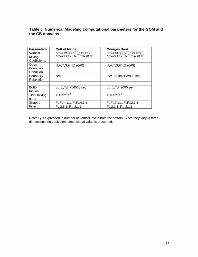
37

Table 6. Numerical Modeling computational parameters for the GOM and the GB domains Parameters Gulf of Maine Georges Bank Vertical Mixing Coefficients

Av=0.5 cm2s-1; Avcvct = 50 cm2s-1

Kv=0.05 cm2s-1; Kvcvct = 50 cm2s-1

Av=0.5 cm2s-1; Avcvct = 10 cm2s-1

Kv=0.05 cm2s-1; Kvcvct = 10 cm2s-1

Open Boundary Condition

U,V,T,S,Ψ,ω: (ORI) U,V,T,S,Ψ,ω: (ORI)

Boundary Relaxation

N/A Lv=10/3km;Tv=900 sec

Bottom friction

Ld=1;Td=756000 sec Ld=1;Td=9000 sec

Tidal mixing coeff

100 cm2s-1 100 cm2s-1

Shapiro Filter

Fu,Fv:4,1,1; Ft,Fs:4,1,1 Fw:2,5,1; Fψ: 2,1,1

Fu,Fv:2,1,1; Ft,Fs:2,1,1 Fw:2,1,1; Fψ: 2,1,1

Note: Ld is expressed in number of vertical levels from the bottom. Since they vary in three-dimensions, no equivalent dimensional value is presented.

I

References Allen, J.S., R.C. Beardsley, J.O. Blanton, W.C. Boicourt, B. Butman, L.K. Coachman, A.

Huyer, T.H. Kinder, T.C. Royer, J.D. Schumacher, R.L. Smith, W. Sturges, C.D. Winant, 1983. Physical oceanography of continental shelves. Rev. Geophys. Space. Phys., 21, 1149-1181.

Behrens, W.J., C.N. Flagg, 1986. Shelf Edge Exchange Processes – Phase I Hydrography Report July 1983-October 1984. Technical Report, Brookhaven National Laboratory.

Beardsley, R.C., B. Butman, W. R. Geyer and P.C. Smith, 1997. Physical oceanography of the Gulf of Maine, An Update. In Gulf of Maine Ecosystem Dynamics, RARGOM report 97-1, 39-52.

Bigelow, H.B., 1927. Physical Oceanography of the Gulf of Maine. Bull. Bureau Fisheries, U.S., 40, 511-1027.

Bisagni J. J., R. C. Beardsley, C. M. Ruhsam, J. P. Manning and W. Williams, 1996. Historical and recent evidence concerning the presence of Scotian Shelf water on southern Georges Bank. Deep-Sea Research, 43, 1439-1471.

Bisagni, J. J. and P. C. Smith, 1998. Eddy-induced flow of Scotian Shelf water across Northeast Channel, Gulf of Maine. Cont. Shelf Res., 18, 515-539.

Brooks, D. A., 1985. Vernal circulation in the Gulf of Maine. J. Geophys. Res., 90, 4687-4705.

Brooks, D. A., 1987. The influence of warm-core rings on slope water entering the Gulf of Maine. J. Geophys. Res., 92, 8183-8196.

Brooks, D. A. and D. W. Townsend, 1989. Variability of the coastal current and nutrient pathways in the eastern Gulf of Maine. J. Mar. Res., 47, 303-321.

Brooks, D. A., 1990. Currents at Lindenkohl Sill in the southern Gulf of Maine. J. Geophys. Res., 95, 22173-22192.

Brown, W. S. and R. C. Beardsley, 1978. Winter circulation in the western Gulf of Maine, Part 1. Cooling and water mass formation. J. Phys. Oceanog., 8, 265-277.

Brown, W. S. and J. D. Irish, 1992. The annual evolution of geostrophic flow in the Gulf of Maine,1986-1987. J. Phys. Oceanog., 22, 445-473.

Brown, W. S. and J. D. Irish 1993. The annual variation of water mass structure in the Gulf of Maine, 1986-1987. J. Mar. Res., 51, 53-107.

Brown, W. S., 1998a. Wind-forced pressure response of the Gulf of Maine. J. Geophys. Res., 103, 30,661-30,678.

Brown, W.S., 1998b. Boundary flux measurements in the coastal ocean. The Sea, Vol 10, 399-418.

Brown, W.S., F. L. Bub, B.J. Rothschild, M.A. Sundermeyer, A. Gangopadhyay, R. Lane and A. R. Robinson, 2001. Assimilating Near Real Time Fish and Environment Data into an Advanced Fisheries Management Information System. ICES Annual Science Conference, Oslo, Norway, 25-29 September.

Butman, B. and R. C. Beardsley 1987. Long-term observations on the southern flank of Georges Bank. Part I, A description of the seasonal cycle of currents, temperature, stratification and wind stress. J. Phys. Oceanog., 17, 367-384.

II

Butman, B., J.W.Loder, and R.C. Beardsley, 1987. The seasonal mean circulation, Observation and theory, In Georges Bank, ed. R.H.Backus, 125-138. Cambridge. MIT Press.

Carter, E. F. and A. R. Robinson, 1987. Analysis models for the estimation of oceanic fields. J. Atmos. Ocean. Tech., 4,49-74.

Chapman, D. C. and R. C. Beardsley, 1989. On the origin of shelf water in the Middle Atlantic Bight. J. Phys. Oceanog. 19, 384-391.

Chapman, D.C., G.Gawarkiewicz, 1993. On the establishment of the seasonal pycnocline in the Middle Atlantic Bight. J. Phys. Oceanog., 23, 2487.

Chen, C. and R. C. Beardsley, 1995. A numerical study of stratified tidal rectification over finite-amplitude banks. Part I, Symmetric banks. J. Phys. Oceanog., 25, 2090-2110.

Chen, C., R. C. Beardsley, and R. Limeburner, 1995. A numerical study of stratified tidal rectification over finite-amplitude banks. Part II, Georges Bank. J. Phys. Oceanog., 25, 2111-2128.

Cummings, J.A., C. Szczechowski and M. Carnes, 1997 Global and regional ocean thermal analysis systems. Marine Tech. Soc. J., 31, 63-75.

Cushman-Roisin, B.L., 1994, Introduction to Geophysical Fluid Dynamics, Prentice-Hall, Englewood Cliffs, New Jersey 07632.

Flagg, C. N., 1987. Hydrographic structure and variability. Georges Bank. R. H. Backus and D. W. Bourne. Cambridge, MA, MIT Press, 108-124.

Fox D.N., M.R. Carnes and J.L. Mitchell, 1992. Characterizing Major Frontal Systems, A Nowcast /Forecast System for Northwest Atlantic. Oceanography, Vol. 5, No. 1, 49-53.

Gangopadhyay, A., A.R. Robinson, and H.G. Arango, 1997. Circulation and Dynamics of the Western North Atlantic, I, Multiscale Feature Models. J. Atmos. Ocean. Tech., 146, 1314-1332.

Gangopadhyay, A., and A.R. Robinson, 1997. Circulation and Dynamics of the Western North Atlantic, III, Forecasting the Meanders and Rings. J. Atmos. Ocean. Tech., 146, 1352-1365.

Gangopadhyay, A., and A.R. Robinson, 2002. Feature oriented regional modeling of Oceanic Fronts, Dyn. Atmos. Oc., In Press.

Gangopadhyay, A. and S. Lindstorm, 2002. Limited-area feature-oriented modeling in the Gulf Stream SYNOP region, Impact of high horizontal resolution vs. realistic topography, Submitted ms.

Gawarkiewicz, G., F. Bahr, R. C. Beardsley, and K. H. Brink, 2001. Interaction of a Slope Eddy with the Shelfbreak Front in the Middle Atlantic Bight, J. Phys. Oceanog., 31, 2783–2796.

Glenn, S.M., and A.R. Robinson, 1995. Validation of an operational Gulf Stream forecasting model, Qualitative Skill assessment for coastal models, AGU Estuarine/Coastal Series, Vol. 47, American Geophysical Union, 469-499.

Haidvogel, D. B. and A. Beckmann, 1998. Numerical models of the coastal ocean. The Sea. K. H. Brink and A. R. Robinson. New York, John Wiley & Sons, Inc., Vol. 10, 457-482.

III

Haley, P.J. and C.J. Lozano, 1999. Data driven simulations of the circulation in the Gulf of Maine, AFMIS Annual Report, School of Marine Science and Technology, University of Massachusetts Dartmouth, MA.

Halliwell, G.R., Jr., and C.N.K. Mooers, 1979. The space time structure and variability of the shelf water and Gulf Stream surface temperature fronts and associated warm-core eddies. J. Geophys. Res., 84, 7707-7725.

Hannah, C.G., J.W. Loder, and D.G. Wright, 1996. Seasonal variation of the Baroclinic circulation in the Scotia Maine region. In Buoyancy Effects on Coastal and Estuarine Dynamics, Coastal and Estuarine Studies, Vol. 53, 7-29. Published by American Geophysical Union.

Heathershaw, A. D. and Foreman, S. J., 1996. FOAM - a forecasting ocean-atmosphere model for naval applications. J. Defence Science, 1, 434-438.

Hill, A. E., 1998. Buoyancy Effects in Coastal and Shallow Seas, The Sea, K. H. Brink and A. R. Robinson, eds. New York, John Wiley & Sons, Inc., Vol. 10, 21-62.

Holboke, M. J. and D. R. Lynch, 1995. Simulations of the Maine Coastal Current. Proceedings of ASCE 4th International Conference on Estuarine and Coastal Modeling, San Diego, CA, October 1999, 12 pp.

Horne, E.P.W., J.W.Loder, W.G.Harrison, R.Mohn, M.R.Lewis, B.Irwin, and T.Platt, 1989. Nitrate supply and demand at the Georges Bank tidal front, Bulletin of Marine Science, 532-3, 145-158.

Houghton, R. W., R. Schlitz, R.C. Beardsley, R. Butman, and J. Lockwood Chamberlin, 1982. The middle Atlantic bight cold pool, Evolution of the temperature structure during summer 1979. J. Phys. Oceanog., 12, 1019-1029.

Hurlburt, H.E., A.J. Wallcraft, W.J. Schmitz, Jr., P.J. Hogan and E.J. Metzger, 1996. Dynamics of the Kuroshio/Oyashio current system using eddy-resolving models of the North Pacific Ocean, J. Geophys. Res., 101, 941-976.

Johns T.C., Carnel, R. E., Crossley, J. F., Gregory, J. M., Mitchell, J. F. B., Senior, C. A., Tett, S. F. B. and Wood, R. A., 1997. The second Hadley Centre coupled ocean-atmosphere GCM, Model description, spinup and validation. Climate Dynamics, 13, 103-134.

Lermusiaux, P.F.J., 1999a. Estimation and study of mesoscale variability in the Strait of Sicily, Dyn. Atmos. Oc., 29, 255-303.

Lermusiaux, P.F.J., 1999b. Data Assimilation via Error Subspace Statistical Estimation, Part II, Mid-Atlantic Bight Shelfbreak Front Simulations and ESSE Validation. Mon Wea Rev, Vol. 1278, 1408-1432.

Lermusiaux, P.F.J., C.-S. Chiu and A.R. Robinson, 2001. Modeling uncertainties in the prediction of acoustic wavefield in a shelfbreak environment, Proc. of the 5th international conference on theoretical and computational acoustics, May 21-25, 2001. Beijing, China, in press.

Linder, C.A. and G.Gawarkiewicz, 1998. A climatology of the shelfbreak front in the Middle Atlantic Bight, J. Geophys. Res., 103 (C9), 18,405-18,424.

Loder, J. W., 1980. Topographic rectification of tidal currents on the sides of Georges Bank. J. Phys. Oceanog., 10, 1399-1416.

Loder, J. W. and D. A. Greenberg, 1986. Predicted positions of tidal fronts in the Gulf of Maine region. Cont. Shelf Res., 6, 397-414.

IV

Loder, J. W., D. Brickman, and E.P.W. Horne, 1992. Detailed structure of currents and hydrography on the northern side of Georges Bank. J. Geophys. Res., 97, 14331-14351.

Loder, J.W., B. Petrie and G. Gawarkiewicz, 1998. The coastal ocean off Northeastern North America, A large-scale view, The Sea, Vol. 11, 125-134.

Lozano, C.J., A. Robinson, H.G. Arango, A. Gangopadhyay, N. Q. Sloan, III, P.J. Haley, Jr., L. Anderson, and W. Leslie, 1996. An Interdisciplinary Ocean Prediction System, Assimilation Strategies and Structured Data Models, in Modern Approaches to Data Assimilation in Ocean Modeling, Ed. P. Malanotte-Rizzoli, Elsevier Sciences.

Lynch, D. R., 1999. A review of modeling in the Gulf of Maine. Naval Research Review, Vol. 61(1).

Lynch, D. R., F. E. Werner, D.A. Greenberg and J.W. Loder, 1992. Diagnostic model for baroclinic, wind-driven and tidal circulation in shallow seas. Cont. Shelf Res., 12, 37-64.

Lynch, D. R., J. T. C. Ip, C.E. Naimie and F.E. Werner, 1996. Comprehensive coastal circulation model with application to the Gulf of Maine. Cont. Shelf Res., 16, 875-906.

Mavor T. and P. Huq, 1996, Propagation velocities and Instability development of a coastal current, In Buoyancy Effects on Coastal and Estuarine Dynamics, Coastal and Estuarine Studies, Vol 53, 59-70. Published by American Geophysical Union.

McGillicuddy, D.J. Jr., D.R. Lynch, A.M. Moore, W.C. Gentleman, C.S. Davis and C. Meise, 1998. An adjoint data assimilation approach to the estimation of Pseudocalanus spp. population dynamics in the Gulf of Maine-Georges Bank region. Fisheries Oceanography, Vol.7, Nos.3-4, 205-218.

Mountain, D. G. and P. F. Jessen, 1987. Bottom waters of the Gulf of Maine, 1978-1983. J. Mar. Res., 45, 319-345.

Mountain, D.G., 1991. The volume of shelf water in the Middle Atlantic Bight, Seasonal and interannual variability, 1977-1987. Cont. Shelf Res., 11, 251-267.

Mountain, D. G. and J. P. Manning, 1994. Seasonal and interannual variability in the properties of the surface waters of the Gulf of Maine. Cont. Shelf Res., 14, 1555-1581.

Naimie, C. E., J. W. Loder, and D.R. Lynch, 1994. Seasonal variation of the three-dimensional residual circulation on Georges Bank. J. Geophys. Res. 99, 15967-15989.

Naimie, C. E., 1995. On the modeling of the seasonal variation in the three-dimensional circulation near Georges Bank. Ph.D. Thesis, Dartmouth College, Hanover, NH 03755, 257 p.

Naimie, C. E., 1996. Georges Bank residual circulation during weak and strong stratification periods, Prognostic numerical model results. J. Geophys. Res., 101, 6469-6486.

Orlanski, I., 1976, A simple boundary condition for unbounded hyperbolic flows. J. Comp. Phys., 21, 251-269.

Pettigrew, N. R., D. W. Townsend, huijie Xue, J.P. Wallinga, P.J. Brickley and R.D. Hetland, 1998. Observations of the Eastern Maine Coastal Current and its offshore extensions in 1994. J. Geophys. Res., 103, 30,623-30,639.

V

Ramp, S. R., R. J. Schlitz, and W.R. Wright, 1985. The deep flow through the Northeast Channel, Gulf of Maine. J. Phys. Oceanog., 15, 1790-1808.

Robinson, A.R. and W.G. Leslie, 1985. Estimation and Prediction of Oceanic fields, Progr. in Oceanog., 14, 485-510.

Robinson, A.R., M.A. Spall and N. Pinardi, 1988, Gulf Stream simulations and the dynamics of ring and meander processes. J. Phys. Oceanog., 18, 1811-1853.

Robinson, A. R., S.M. Glenn, M.A. Spall, L.J. Walstad, G.M. Gardner, and W.G.Leslie, 1989. Forecasting meanders and Rings, EOS. Ocenogr. Report, 7045, 1464-1473.

Robinson, A.R., 1996. Forecasting and simulating coastal ocean processes and variabilities with the Harvard Ocean Prediction System, Coastal Ocean Processes, C.N.K. Mooers, ed., Coastal and Estuarine Studies, AGU, pp. 77-100.

Robinson, A.R., and A. Gangopadhyay, 1997. Circulation and Dynamics of the Western North Atlantic, II, Dynamics of Meanders and Rings. J. Atmos. Ocean. Tech., 146, 1333-1351.

Robinson, A. R., P. F. J. Lermusiaux, and N.Q. Sloan, III., 1998. Data Assimilation. The Sea, K. H. Brink and A. R. Robinson. New York, John Wiley & Sons, Inc., Vol. 10, 541-594.

Robinson, A.R. 1999 Forecasting and and simulating coastal ocean processes and variabilities with the Harvard Ocean Prediction System, in Coastal Ocean Prediction, C.N.K. Mooers, Ed., AGU Coastal and Estuarine Studies Series, 77-100.

Robinson, A. R. and S.M. Glenn, 1999. Adaptive Sampling for Ocean Forecasting. Naval Research Reviews, 512, 28-38

Robinson, A.R. and the LOOPS Group, 1999. Realtime Forecasting of the Multidisciplinary Coastal Ocean with the Littoral Ocean Observing and Predicting System LOOPS, Preprint Volume of the Third Conference on Coastal Atmospheric and Oceanic Prediction and Processes, 3-5 November 1999, New Orleans, LA, American Meteorological Society, Boston, MA.

Robinson, A.R, B. J. Rothschild, W.G. Leslie, J.J. Bisagni, M.F. Borges, W.S. Brown, D. Cai, P. Fortier, A. Gangopadhyay, P.J. Haley, Jr., H.S. Kim, L. Lanerolle, P.F.J. Lermusiaux, C.J. Lozano, M.G. Miller, G. Strout and M.A. Sundermeyer, 2000. The development and demonstration of an Advanced Fisheries Management Information System. AMS Annual meeting, January 2001.

Simpson, J. H. and J. R. Hunter, 1974. Fronts in the Irish Sea. Nature, 250, 404-406. Sloan, N.Q.S., III, 1996. Dynamics of a shlef-slope front, Process Studies and data-driven

simulations in the Middle Atlantic Bight. Ph.D.Thesis, Harvard University, Cambridge, MA, USA.

Smith, P. C., 1989. Seasonal and interannual variability of current, temperature and salinity off southwest Nova Scotia. Canadian J. Fisheries and Aquatic Sciences, 46, 4-20.

Spall, M.A. and A.R. Robinson, 1990. Regional primitive equation studies of the Gulf Stream meander and ring formation region, J. Phys. Oceanog., 207, 905-1016.

Sundermeyer, M.A., B.J. Rothschild, and A.R. Robinson, 2001. A study of environmental indicators and the predictability of commercial fish stocks, Part II, Coupled bio-physical models, in prep.

VI

Teague, W.J., M.J. Carron, and P.J. Hogan, 1990. A comparision between the Generalized Digital Environmental Model and Levitus climatologies, J. Geophys. Res., 95(C5), 7167-7183..

Watts, D. R., K. L. Tracy and A. I. Friedlander, 1989. Producing accurate maps of the Gulf Stream thermal front using objective analysis. J. Geophys. Res., 94, 8040-8052.

Wright,W.R., 1976. The limits of shelf water south of cape cod, 1941 to 1972. J. Mar. Res., 34, 1-14.

Wright, D. G., D. A. Greenberg, J.W. Loder and P.C. Smith, 1986. The steady-state barotropic response of the Gulf of Maine and adjacent regions to surface wind stress. J. Phys. Oceanog., 16, 947-966.

Xue, H., F. Chai and N.R. Pettigrew, 2000. A model study of the seasonal circulation in the Gulf of Maine. J. Phys. Oceanog., 30, 1111-1135.

i

Figure Captions for ‘Feature-oriented regional modeling and simulation in the Gulf of Maine and Georges Bank’ Keywords: Shelf Seas, Ocean Circulation, Coastal Currents, Shelf Fronts, Gyres and Modeling. Figure 1. (a) A schematic of circulation features in the Gulf of Maine. GSC = Great South Channel; SSF = Shelf/Slope Front; NEC = Northeast Channel; GBG = Georges Basin Gyre; TMF = Tidal Mixing Front; WBG = Wilkinson Basin Gyre; MCC = Maine Coastal Current; JBG = Jordan Basin Gyre. (b) A three-dimensional bathymetric perspective of the regional circulation features. The basins are the three deep regions in the interior Gulf. The vertical mixing region is predominantly in the Wilkinson Basin. Figure 2. Multi-scale nested modeling domains for the western north Atlantic. The Northwest Atlantic (NWA) domain has a horizontal resolution of 15-km with triple-nested domains in: Gulf of Maine (5-km resolution), Georges Bank (5/3-km) and Massachusetts Bay (5/3-km). Feature-oriented initialization and updating helps in transferring information between such regions through multiscale circulation structures, which exist, evolve and interact over these domains in a dynamical model. Figure 3. A schematic representation of a coastal current/front temperature-salinity feature model. It is defined by horizontal gradients of the tracer (temperature/salinity) as shown in (a) and a vertical structure φ(x,z), which varies with alongstream distance(x) as shown in (b). See Equations (1) and (2) in text. Figure 4. Water mass properties for feature model of Maine Coastal Current near Scotia Shelf at the axis. (a) Monthly average temperature vs. depth; (b) Monthly average salinity vs. depth for different months; (c) T vs. S for different months; and (d) Variation of the T-S property along the Coastal Current during the month of June. The black-blue-green-red variation depicts the transition of Maine Coastal Current t-s from being cold and fresh near Scotian Shelf (black) to eastern (blue), to western (green) gulf, and finally to warm and salty outflow (red) near GSC. The variability in (d) shows the relevance of using the alongstream and cross-stream gradient formulation as in Eq. (1). Figure 5. Water mass properties for feature model of the Georges Bank Northern Flank front axis are shown in: (a) Monthly average temperature vs. depth; and (b) Monthly average salinity vs. depth for different months. Similar profiles for the frontal axis on the southern flank of Georges Bank are shown in (c) Monthly average temperature vs. depth; and (b) Monthly average salinity vs. depth for different months.

ii

Figure 6. Monthly T-S variation for the (a) northern and (b) southern flank fronts around Georges Bank. Each color represents a particular month. Figure 7. Monthly T-S variation for the (a) Central Georges Bank; and the three basins: (b) Wilkinson Basin; (c) Georges Basin; and (d) Jordan Basin. Figure 8. Water mass properties for feature model of the three basins in the interior Gulf of Maine. Monthly average temperatures vs. depth profiles are shown for (a) Wilkinson, (b) Georges and (c) Jordan basins. Similarly, monthly average salinity-depth profiles are shown (d) Wilkinson, (e) Georges and (f) Jordan basins. Figure 9. Locations of certain available observational synoptic sections are shown here. Data from these sections were used for feature modeling the three gyres in the summertime simulations.

Figure 10. A synoptic feature-oriented circulation template for the GOMGB region used for initialization and updating of numerical models is presented here. The red marks are pseudo-CTD stations where feature model t-s profiles are generated. The profile locations are strategically selected along and across circulation features such as the Maine Coastal Current, the Tidal mixing front, the shelf-slope front, the Northeast Channel inflow, the Great south Channel outflow, and the three basins, Wilkinson, Jordan and Georges. Figure 11. (a) Distribution of profiles, which were used as background climatology for melding with feature model profiles in Figure 10. The NWA shelf climatology for RTDOC of AFMIS during March-April 2000 was derived from NODC and NMFS data sets. (b) A typical coarse (1˚) resolution climatological data sets available form GDEM is shown here. Figure 12. Initialization fields of temperature (upper left) and salinity (upper right) at the surface for the Gulf of Maine domain simulation. Similar fields are shown in the bottom panels at a depth of 10m (level 3). Superimposed velocity vectors are also shown at the corresponding levels. Figure 13. A 10-day long simulation of temperature (color) superimposed with velocity vectors in the Gulf of Maine domain is shown here. This run was initialized with fields presented in Figure 12. Fields are for days 1, 4, 7 and 10. Note the robustness of the cyclonic gyre on the Jordan Basin and the coastal current system along the coast. The shelf-slope front meanders and generates mesoscale and submesoscale features during this simulation.

iii

Figure 14. Georges Bank simulation at high resolution (5/3 km) starting on April 9, 2000. Temperature and superimposed velocity fields are shown for Nowcast and days 3, 6 and 9. Note the robustness of the TMF on the northern flank compared to the simulation results in Figure 13. Such simulations indicates the potential of using a feature-oriented approach for mesoscale nowcasting and forecasting in the coastal regions. Figure 15. Three-day simulated fields of temperature and velocity from a summer, 2001 Gulf of Maine simulation forced with winds. Upper panel shows the nowcast and 1-day forecast and the lower panel shows the forecasts on days 2 and 3. Figure 16. (a) Wind stress (dynes/cm2); (b) Heat Flux (W/m2); and (c) Evaporation – Precipitation (cm/day) fields from the FNMOC Nowcast field. (d) wind-stress field on day 1 from the FNMOC model forecast. These fields were used to force the operational model initialized with FORMS during summer of 2001 for synoptic forecasting and sensitivity studies. Figure 17. Difference fields for sensitivity to different forcing fields. (a) Wind stress forced simulation – unforced simulation; (b) Wind stress and Heat flux forced simulation – unforced simulation; (c) Wind stress + Heat flux forced simulation – Wind stress forced simulation. The last panel (d) shows the difference in salinity field between wind stress + heat flux + (E-P) forced simulation and (wind stress + heat flux) forced simulation. In short, impact of wind stress, wind stress + heat flux, heat flux and (E-P) are shown in Figures (a), (b), (c), and (d) respectively.