1

FEATURE EXTRACTION FOR DATA INPUT TO NEURO-CLASSIFIERS

Talk on MMPC-2009 Dubna LIT JINR, 7 July2009

Gennady OsoskovDmitry Baranov

Laboratory of Information TechnologiesJoint Intstitute for Nuclear Research,

141980 Dubna, Russiaemail: ososkov@jinr.ru

G.Ososkov

2

Why ANN for contemporary HEP experimentsArtificial neural networks (ANN) are widely and

successfully used for solving problems of classification, forecasting, and recognition in many scientific applications, in particular and especially in high energy physics (HEP).

Moreover, namely physicists wrote in late 80-ties one of the first NN programing packages – Jetnet. They were also among first neuro-chip users.

Main reasons were:• The possibility to generate training samples of any arbitrary needed length by Monte Carlo on the basis of some new physical model• neuro-chip appearance on the market at that time which make feasible implementing a trained NN, as a hardware for the very fast triggering and other NN application.

Brief reminder of ANN basic concepts

1. Feed-forward ANN (MLP or RBF- networks)

Artificial neuron

2. Fully-connected or recurrent ANN

Output-layer neurons transform hidden neurons hj asThen training sample ({xi}(m), {zi}(m) )

is needed to train MLP to obtain weights bythe error backpropagation algorithm

E=ΣmΣij (yi (m) – zi

(m) )2 → min{wik} which is based on the steepest descent method.

the i-th neuron output signalhi=g(Σjwij sj)

Activation function g(x)

∑=k

kkjj hwgy )(

The “curse of dimensionality” problem arises in many non-physics applications due to

very high dimensionality of experimental data to be classifiedthe amount of these data is scarce for training and quality verification of a trained network

3

4

Example: Genetics of proteinsRadiobiology study The genetics of gliadin (alcohol soluble protein)

have been studied in detail by a special gel electrophoresis. Each electrophoretogram strip after its digitalization became a densitogramspectrum consisting of about 4000 pixels.

Electrophoregram examplewith 17 wheat cultivar It can be considered as a simple genetic formula,

which allows for a qualified expert to classify any spectrum to its corresponding protein.

Such classifying procedure is of great importance in radiobiology and, especially, in agriculture

Therefore it is to be automatized.

5

Genetics of protein (continue)The problem: realize ANN based expert system to identify the wheat cultivar

by its spectrum.Note: the electrophoregram information must be considerably preprocessed to

suit as input to an expert system Preprocessing stages:1. digitization and standardization of densitometry data

- smoothing, denoising and eliminating background pedestal;

- density normalization to the range 0-255;- aligning all strip to fix the beginning and the end of information on each gel

(was fulfilled by Hamming neural net)

2. extracting most informative features

6

Curse of dimensionality problemInput: 4000 pixelsOutput: 5 ÷ 20 sorts to be classifiedMLP dimension D=4000*1000+1000*20=4.2 *106, i.e millions of weightsor equations to solve by the error back propagation method!A cardinal reduction of input data was needed

Feature extraction approachesFeature extraction approaches1st approach: spectrum coarsing from 4000 points into 200 zones with averaged density (D=16400 weights)The real size of the training sample is 120 etalons preliminarily classified by experts for each of 20 wheat sorts, i.e. for 5 different sorts we have 600 etalons for training.Result for 5 sorts: after training ANN (200/80/5) the efficiency was 85%.

2d Fast Fourier transform (FFT). Real part of direct FFT was used totransform input data to the frequency domain, where the highest frequencies were cut up to 256 (16 times of reduction)

After transforming all training samples to Fourier space NN-classifier (256/40/5) was trained on them and tested again on transformed sample.Result for 5 sorts: 100% of efficiency

Feature extraction approaches (contin)3d. Principal component analysis (PCA) transforms d-dimensional data to a m-dimensional subspace by using the information of their covariance matrix SX=cov(XiXk). The orthogonal Karhunen–Loeve transform gives the diagonal form of SX with eigenvalues li numbered in decreasing order. Thus, we can retain only m most significant eigenvalues l1, l2, …, lm (m « p) and express the input data in terms of these principal components as

PCA has its neural network implementations what allows to avoid cumbersome calculations of covariance matrices and their eigenvectors. It is done by so-called recircular (autoassociative) NN. Such NN uses 4000 input neurons, as etalon, output ones. The number of hidden neurons Nhid should correspond to the number of principal components. The best efficiency of the next classifying network was obtained for Nhid =150,i.e. data compression in more than 20 times.

....2211 mmiiii YlYlYlX +++≅

Original spectrum restored spectrum

(PCA in its NN form was also successfully used for the face recognition)Result for 5 sorts: after extracting 150 PC from all data of training and testing samples the PCA classifying efficiency was 99,54%. This efficiency keeps stable while the increase of sorts number till 8 then drops down for 17-25%

7

8

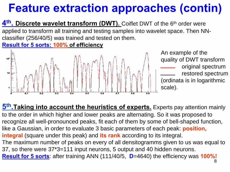
Feature extraction approaches (contin)4th. Discrete wavelet transform (DWT). Coiflet DWT of the 6th order were applied to transform all training and testing samples into wavelet space. Then NN-classifier (256/40/5) was trained and tested on them.Result for 5 sorts: 100% of efficiency

An example of the quality of DWT transform

original spectrumrestored spectrum

(ordinata is in logarithmic scale).

5th.Taking into account the heuristics of experts. Experts pay attention mainly to the order in which higher and lower peaks are alternating. So it was proposed to recognize all well-pronounced peaks, fit each of them by some of bell-shaped function, like a Gaussian, in order to evaluate 3 basic parameters of each peak: position, integral (square under this peak) and its rank according to its integral. The maximum number of peaks on every of all densitogramms given to us was equal to 37, so there were 37*3=111 input neurons, 5 output and 40 hidden neurons.Result for 5 sorts: after training ANN (111/40/5, D=4640) the efficiency was 100%!

9

On the basis of this study software system was elaborated in the collaboration with the Vavilov Institute of General Genetics RAS (VIGG RAS) for the full chain of genetic analysis of electrophoregrams including the preprocessing stage. The system is now in use for testing and further developing. Results for higher number of sorts shows:

Notable decrease of the classifying efficiency;a preference of the ranking method

The main reasons are1. Spectrum variability for the same sort

Efficiency in %

RankingFourier and DWT

2. Spectrum similarity for genetically close sorts

Spectra for the wheat cultivar #19

Status of the wheat protein classificationStatus of the wheat protein classification

Number of sortsSort # 6# 13#19 # 26

Therefore, the further development is thought

to apply Kohonen SOM ANN and to formalize expert classifying approaches in order to elaborate a hierarchy of NN for the wheat protein classification.

10

Summary1. A comparative study of the feature extraction methods was

fulfilled on the example of wheat protein genetic classification2. 5 different methods were tested

- coarsing data to 200 zones with mean density;- PCA by recircular network;- FFT;- DWT; - ranking data by peak integral.

3. Last four methods show satisfactory results on classifying 5 sorts4. Further increasing sort numbers causes drop of classifying

efficiency, ranking method showed its advantage. 5. Software system was elaborated in collaboration with the VIGG

RAS Institute for the full chain of electrophoretic data genetic analysis.

6. Further system development is in progress.Authors thank Dr.A.Kudryavtsev (VIGGS) for the problem formulation and providing

all experimental data and also S.Lebedev, S.Dmitrievsky, and E.Demidenko(JINR) for the essential help in performing calculations.

11

Thanks for your attention!Thanks for your attention!

12

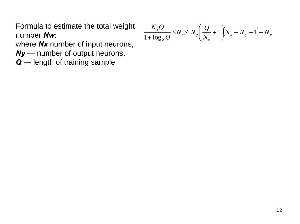
Formula to estimate the total weight number Nw: where Nx number of input neurons,Ny — number of output neurons,Q — length of training sample

( ) yyxx

ywy NNN

NQNN

QQN

+++⎟⎟⎠

⎞⎜⎜⎝

⎛+≤≤

+11

log1 2

13

Brief introduction to waveletsOne-dimensional wavelet transform (WT) of the signal f(x) has 2D form

where the function Ψ is the wavelet, b is a displacement (shift), and a is a scale.Condition Cψ < ∞ guarantees the existence of Ψ and the wavelet inverse transform. Due to freedom in Ψ choice, many different wavelets were invented.The family of continuous wavelets is presented here by Gaussian wavelets, which are generated by derivatives of Gaussian function

Two of them, we use, are

and

Most knownwavelet G2 is named

“the Mexican hat”

14

Wavelets can be applied for extracting very special features of mixed and contaminated signal

G2 wavelet spectrum of this signal

Filtering results. Noise is removed and high frequency part perfectly localized

An example of the signal with a localized high frequency part and considerable contamination

then wavelet filtering is applied

Filtering works in the wavelet domain bythresholding of scales, to be eliminatedor extracted, and then by makingthe inverse transform

15

Continuous wavelets: pro and contraPRO: - Using wavelets we overcome background estimation

- Wavelets are resistant to noise (robust)

CONTRA: - redundancy → slow speed of calculations - nonorthogonality (signal distotrs after inverse transform)

Besides, real signals to be analised by computer are discrete,So orthogonal discrete wavelets should be preferable.

The discrete wavelet transform (DWT) was built by Mallat as multi-resolution analysis. It consists in representing a given data as a signal decomposition into basis functions φand ψ. Both these functions must be compact in time/space and frequency domains.

Scheme of one step of the wavelet decomposition and reconstruction

16

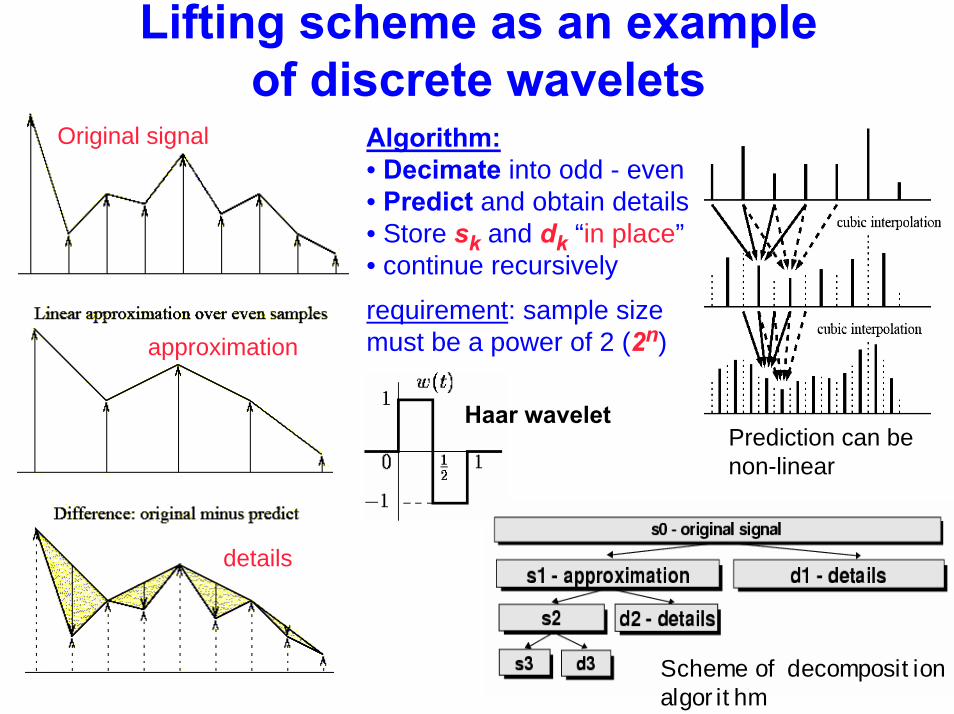
Lifting scheme as an exampleof discrete wavelets

Scheme of decomposition algorithm

Algorithm:• Decimate into odd - even• Predict and obtain details• Store sk and dk “in place”• continue recursively

requirement: sample sizemust be a power of 2 (2n)

Original signal

Haar wavelet

details

approximation

Prediction can be non-linear

17

Various types of discrete wavelets

Daubechie’s waveletwith 2 vanishing momenta Coiflet – most symmetricBi-orthogonal

CDF44 wavelet

Denoising by DWT shrinkingwavelet shrinkage means, certain wavelet coefficients are reduced to zero:

Our innovation is the adaptive shrinkage,i.e. λk= 3σk where k is decomposition level (k=scale1,...,scalen), σk is RMS of Wψ for this level (recall: sample size is 2n)

An example of Daub2 spectrum