Feature-based Quality Assessmentof Spoof Fingerprint ImagesMaster’s thesis in Biomedical Engineering

JENNY NILSSON

Department of Signals and SystemsCHALMERS UNIVERSITY OF TECHNOLOGY

Gothenburg, Sweden 2017

Master’s thesis 2017:01

Feature-based Quality Assessmentof Spoof Fingerprint Images

JENNY NILSSON

Department of Signals and SystemsSignal Processing and Biomedical EngineeringComputer Vision and Medical Image Analysis

Chalmers University of TechnologyGothenburg, Sweden 2017

Feature-based Quality Assessment of Spoof Fingerprint ImagesJENNY NILSSON

© JENNY NILSSON, 2017.

Supervisor: Jennifer Alvén, Department of Signals and SystemsSupervisor: Olof Enqvist, Department of Signals and SystemsSupervisor: Kenneth Jonsson, Fingerprint Cards ABExaminer: Fredrik Kahl, Department of Signals and Systems

Master’s Thesis 2017:01Department of Signals and SystemsSignal Processing and Biomedical EngineeringComputer Vision and Medical Image AnalysisChalmers University of TechnologySE-412 96 GothenburgTelephone +46 31 772 1000

Cover: Example fingerprint images. The left one is a fingerprint image created byplacing a synthetic fingerprint on the fingerprint sensor and the right one is createdby placing the live finger on the fingerprint sensor. The two fingerprint imagesoriginate from the same fingerprint area.

Gothenburg, Sweden 2017

iv

AbstractFingerprint recognition has over the last decade become a natural component inmodern identity management systems. As the commercial use of fingerprint recog-nition systems increases, the benefits from attacking such systems become greater.The security of a biometric system is seriously compromised if the system is un-able to differentiate between a real and a counterfeit fingerprint. From this securitythreat, a need for methods to prevent or detect such spoofing attacks has emerged.

This thesis is concerned with so called liveness detection, that is the process ofdetermining whether a captured fingerprint is fake or not. More precisely, the thesisexplores different ways to assess how difficult it is to correctly classify a set of fakefingerprint images. Differences in image characteristics between the two classes arealso explored. The purpose of the thesis is to design a quality assessment tool forfake fingerprint images used in the liveness algorithm development at FingerprintCards. The quality assessment tool aims to give an indication of how difficult a setof such ’spoof’ images are to classify based on the evaluated liveness characteristics.

In the first part of the thesis, features which differ between images of genuineand fake fingerprints are designed. Based on these designed liveness features, asupport vector machine classifier is created by identifying the hyperplane modelwhich best separates the images of living and spoof fingerprints. The quality of aspoof image data set is defined as the number of spoof images that this hyperplanemodel manages to classify correctly. Further, the quality of each individual spoofimage is defined as the liveness probability assigned by the hyperplane model.

Promising results were obtained from the quality assessment tool developed inthe first part of the thesis. The spoof images that were assigned a low qualityby the hyperplane model were images which easily could be differentiated fromtheir live equivalents in a manual inspection. Conversely, the spoof images thatwere assigned a high quality were images in which the fingerprint patterns couldnot be differentiated from live fingerprint patterns. Hence, these results indicatea successfully designed spoof quality assessment. Further, it shows that manuallydesigned liveness features can be used to estimate the spoof image quality.

In the second part of the thesis, a deep fine-tuned convolutional neural network isevaluated for quality assessment of spoof images. The utilized network has recentlyobtained state-of-the-art results in fingerprint liveness detection. If the deep neuralnetwork cannot differentiate between the live and fake images in a set, the images areconsidered very hard to classify. Conversely, if a shallow network easily differentiatesspoof images from live images, these images are considered easy to classify.

The liveness classification results obtained in the second part of the thesis werefar better than expected. The fine-tuned convolutional neural network demonstratedfantastic liveness classification results by classifying all images in the test set cor-rectly. These results imply that all the images in the set are possible to classifyproperly. However, the fact that the network managed to classify even the mostrealistic spoof images correctly with a high degree of certainty makes this networkarchitecture unsuitable for spoof quality assessment. Differentiation between theimages in the set could however possibly be obtained with a more shallow network.

Keywords: secure identity management, biometric recognition, fingerprints, spoof-ing attacks, liveness detection, spoof fingerprint image quality, liveness feature ex-traction, convolutional neural networks.

v

AcknowledgementsI would first like to acknowledge Kenneth Jonsson for giving me the opportunityto work with this master thesis project. Further, I would like to thank the entireAlgorithm group at Fingerprint Cards, Gothenburg, for introducing me to the fieldsof fingerprint recognition and liveness detection and for all the help and valuablediscussions along the way. I would also like to thank all other staff at FingerprintCards, Gothenburg, for the warm welcome and for showing interest in my thesiswork. Moreover, I would like to sincerely thank my academic supervisors, JenniferAlvén and Olof Enqvist, for their expertise, guidance and support throughout theproject. It has been a pleasure working with all of you. Lastly, I would like to thankmy friends and family, especially Filip, for your unconditional support during mystudies at Chalmers. Without you I would not have come this far.

Jenny Nilsson, Gothenburg, January 2017

vii

Contents

1 Introduction 11.1 Problem description . . . . . . . . . . . . . . . . . . . . . . . . . . . 21.2 Contribution . . . . . . . . . . . . . . . . . . . . . . . . . . . . . . . 31.3 Scope . . . . . . . . . . . . . . . . . . . . . . . . . . . . . . . . . . . 31.4 Related work . . . . . . . . . . . . . . . . . . . . . . . . . . . . . . . 3

2 Theory 52.1 Fingerprints . . . . . . . . . . . . . . . . . . . . . . . . . . . . . . . . 5

2.1.1 Fingerprint formation . . . . . . . . . . . . . . . . . . . . . . 52.1.2 Fingerprint representation . . . . . . . . . . . . . . . . . . . . 62.1.3 Fingerprint sensing . . . . . . . . . . . . . . . . . . . . . . . . 72.1.4 Fingerprint spoofing . . . . . . . . . . . . . . . . . . . . . . . 8

2.2 Fingerprint image pre-processing . . . . . . . . . . . . . . . . . . . . 92.2.1 Segmentation . . . . . . . . . . . . . . . . . . . . . . . . . . . 92.2.2 Fingerprint orientation . . . . . . . . . . . . . . . . . . . . . . 92.2.3 Binarization . . . . . . . . . . . . . . . . . . . . . . . . . . . . 102.2.4 Morphological operations . . . . . . . . . . . . . . . . . . . . 102.2.5 Minutiae extraction . . . . . . . . . . . . . . . . . . . . . . . 12

2.3 Learning-based feature extraction . . . . . . . . . . . . . . . . . . . . 13

3 Methods 153.1 Feature design for fingerprint liveness classification . . . . . . . . . . 15

3.1.1 Registration . . . . . . . . . . . . . . . . . . . . . . . . . . . . 163.1.2 Visual interpretation . . . . . . . . . . . . . . . . . . . . . . . 173.1.3 Segmentation . . . . . . . . . . . . . . . . . . . . . . . . . . . 173.1.4 Fingerprint orientation . . . . . . . . . . . . . . . . . . . . . . 183.1.5 Fingerprint binarization . . . . . . . . . . . . . . . . . . . . . 193.1.6 Fingerprint skeletons . . . . . . . . . . . . . . . . . . . . . . . 193.1.7 Fingerprint intensities . . . . . . . . . . . . . . . . . . . . . . 223.1.8 Ridge and valley width . . . . . . . . . . . . . . . . . . . . . 233.1.9 Statistical significance . . . . . . . . . . . . . . . . . . . . . . 253.1.10 Spoof image quality . . . . . . . . . . . . . . . . . . . . . . . 25

3.2 Learning-based fingerprint liveness classification . . . . . . . . . . . . 26

4 Experimental results and analysis 314.1 Feature design for fingerprint liveness classification . . . . . . . . . . 31

4.1.1 Visual interpretation . . . . . . . . . . . . . . . . . . . . . . . 314.1.2 Segmentation . . . . . . . . . . . . . . . . . . . . . . . . . . . 32

ix

Contents

4.1.3 Skeleton-based features . . . . . . . . . . . . . . . . . . . . . 334.1.4 Intensity distributions . . . . . . . . . . . . . . . . . . . . . . 404.1.5 Ridge and valley width . . . . . . . . . . . . . . . . . . . . . 444.1.6 Spoof image quality . . . . . . . . . . . . . . . . . . . . . . . 48

4.2 Learning-based fingerprint liveness classification . . . . . . . . . . . . 504.2.1 Network trained on benchmark data . . . . . . . . . . . . . . 504.2.2 Network trained on Fingerprint Cards data . . . . . . . . . . 51

5 Conclusion 55

Bibliography 57

x

1Introduction

Identity management is an essential element in a large number of societal applica-tions today. As concerns about the security in many of these applications increase,so does the need for systems which reliably assess the identity of its users. Examplesof applications in which the demand for secure identity establishment is particularlyhigh are regulation of international border crossings, access control to importantfacilities or privileged information as well as electronic access control and transac-tions. Since traditional knowledge and token-based credentials such as passwords,keys, cards and passports can be shared, guessed, misplaced or stolen, they cannotbe fully trusted to establish identities. Thus, these traditional identity managementsystems often fail to meet high demands on performance and security [1].

Biometric recognition has over the last decades been increasingly deployed as analternative or supplement to traditional systems and has now become a naturalcomponent in authorization and identification systems. Since biometric recognitionsystems are based on the premise that all individuals possess distinctive anatomicaland behavioral characteristics from which they uniquely can be associated with anidentity, these systems are generally agreed to be a reliable and powerful tool inmodern identity management. The biometric characteristics most commonly usedtoday are fingerprints, faces and irises and since biometric identifiers intrinsicallyrepresent the bodily identity of an individual they can neither be misplaced, sharednor stolen. Consequently, person recognition systems utilizing identifiers that intrin-sically are linked to the user are considered to be superior to traditional knowledgeor token-based methods, both in terms of security and user convenience [1, 2].

Even though biometric recognition systems are based on identifiers unique for allusers, this fact does not make them immune to fraudulent attacks. In general, thereare two ways to circumvent a biometric system, either by direct or indirect attacks.Indirect attacks refer to the type of attack performed inside the system, such asmanipulation of the feature extraction or feature matching modules and modifi-cation of the database containing enrolled feature sets. Since indirect attacks areperformed within the digital limits of the system they can be prevented by digitalprotection mechanisms like anti-virus software, encryption, firewalls and intrusiondetection. The type of attacks performed outside the digital limits of the system isreferred to as direct attacks. In such attacks the impostor either modifies its biomet-ric identifier to evade identification or poses as a valid user by presenting a forgedbiometric identifier to the sensor in order to illegitimately be granted access to thesystem. The latter of these, the presentation of a counterfeit biometric identifier tothe sensor, is commonly known as spoofing or presentation attacks. The counterfeit

1

1. Introduction

biometric identifiers used in these attacks are commonly known as spoofs. As spoof-ing neither require any advanced programming skills nor any remarkable alterationsof the intruders own biometric identifiers, it is considered to be the most potent anddamaging type of system attack [3].

As the commercial use of biometric systems increases, the benefits from attackingsuch systems become greater, hence the frequency and intensity of spoofing attacksare expected to increase in the coming years. The security of a biometric systemis of course seriously compromised if the system is unable to differentiate betweena real and a counterfeit biometric identifier. From this security threat a need formethods to prevent or detect spoofing attacks has emerged. Our facial images andvoices are constantly captured by cameras and audio recorders and our fingerprintsand DNA are left wherever we touch, hence our biometric identifiers can in no waybe claimed as secret. Consequently, the security of biometric systems cannot relyon the inaccessibility of our biometric identifiers to potential attackers, but mustinstead take the liveness of the presented sample into account. Thus, most biomet-ric recognition systems now couple their identification or verification process with aspoofing countermeasure module which evaluates the liveness of the presented sam-ple and classifies it either as a real, living sample or as a non-live sample [1, 3].

In fingerprint recognition systems, there are both hardware-based and software-based techniques to evaluate the liveness of a sample. In the hardware-based ap-proaches, additional devices are added to the system to detect different propertiesof the sample that is associated with either live or non-live traits. There are a lot ofways to measure vital signs with hardware-based techniques, a few of many exam-ples are measurement of blood flow, oxygenation of the blood, electrical propertiesor signals, skin perspiration, spectral characteristics or biochemical assays of humantissues as well as changes in skin tone when the finger is pressed against the sensorsurface. It is also possible to detect odors and properties associated with differentspoofing materials. While hardware-based approaches operate directly on the fin-ger, software-based approaches operate on the fingerprint images already obtainedfrom the sensor and make use of differences in features extracted from live samplesand spoofs. Hardware-based techniques generally have a higher performance com-pared to software-based approaches and the best classification performance wouldprobably be obtained by a combination of the two. The additional sensors requiredin hardware-based approaches, however, brings considerable and undesirable addi-tional costs and size to the systems. Thus, software-based approaches are preferablein applications where low cost and small size are significant factors [3].

1.1 Problem description

Fingerprint Cards is a company developing both software and hardware solutionsfor biometric recognition systems based on fingerprint characteristics. One of thesesoftware solutions is an algorithm which evaluates the liveness of fingers presentedto the sensor [4]. Algorithms for liveness detection are often based on feature ex-traction from the fingerprint image and use different machine learning techniquesto classify the presented finger as either live or spoof based on the resulting featurevector. The performance of such a classification algorithm is heavily dependent on

2

1. Introduction

the amount and nature of training data as well as on the characteristics of the datato be classified [2, 5]. Since the algorithm performance is data dependent, it differsfor different data sets due to variations in the data. In order to obtain compa-rable algorithm performance measurements for data sets from different sources, aquantitative quality assessment of the spoof images in the data sets is needed.

1.2 Contribution

This thesis explores different ways to assess how difficult it is to correctly classifya set of fake fingerprint images. The purpose of the thesis is to design a qualityassessment tool for the fake fingerprint images used in algorithm training and eval-uation at Fingerprint Cards. The quality assessment tool aims to give an indicationof how difficult a set of spoof fingerprint images are to classify correctly.

1.3 Scope

In this thesis, two different ways to assess how difficult it is to correctly classify a setof fake fingerprint images are explored. The thesis is thus divided into two parts. Inthe first part of the thesis, features which differ between live and spoof fingerprintimages are designed. These differences will be measured quantitatively and used toestimate the quality of spoof fingerprint images. This part has been limited to onlyconsidering images acquired from one type of sensor, and it has also been limitedto only considering images of spoofs made of wood glue that are fabricated from atwo-dimensional fingerprint capture. In the second part of the thesis, convolutionalneural networks are considered as a possible way of evaluating the spoof fingerprintimage quality. A liveness classifier based on a deep convolutional neural network willbe implemented and the spoof image quality in a given data set will be estimatedfrom the obtained network classification results.

1.4 Related work

The Fingerprint Liveness Detection Competition is a competition which is held ev-ery other year and which compares fingerprint liveness classification methodologiesand establishes the current state-of-the-art in liveness classification. The data setsused in these competitions are publicly available and are used as benchmark datasets in the liveness classification research community [3]. State-of-the-art resultson these data sets using the software-based liveness detection approach has beenreported in [6–9]. The fingerprint liveness classification algorithm presented in [6] isa learning-based classifier which uses convolutional neural networks for fingerprintliveness detection. This algorithm won the last Fingerprint Liveness Detection Com-petition which took place in 2015. The algorithm which placed second in the lastFingerprint Liveness Detection Competition was submitted from the research groupbehind [7, 8]. In these articles, a liveness detection method based on local descriptorsand support vector machine classification is proposed. The novel local descriptorproposed in [7] is based on image contrast and phase information extracted locallyfrom the spatial and frequency domains of the image. One of the descriptors inves-tigated in [8], is the same as the local descriptor proposed for fingerprint liveness

3

1. Introduction

classification in [9]. This descriptor encodes the local fingerprint texture to a featurevector by using automatically learned filters. The classification algorithm in [9] is asupport vector machine classifier based on this feature vector. These four method-ologies are however designed for optical fingerprint images, which differ much incharacteristics from the capacitive fingerprint images assessed at Fingerprint Cards.

Various fingerprint-specific image quality features have also been proposed for fin-gerprint liveness classification purposes [10–15]. The fingerprint image quality maybe assessed by measuring the pattern clarity, the pattern continuity, and the pat-tern strength or directionality [10]. The pattern strength has been assessed bothby measuring the fingerprint orientation certainty level [11] and the energy con-centration in the power spectrum [12]. The discriminative power of these livenessfeatures has been found to be high [10]. The pattern clarity has been assessed bymeasuring the mean and standard deviation of the fingerprint image intensities [13],by estimating a local clarity score [14] and by analyzing the amplitude and varianceof the sine waves which form the fingerprint pattern [15]. The pattern continuityhas been assessed both by measuring the local fingerprint orientation quality [14]and the continuity of the fingerprint orientation field [11]. Both the pattern clarityand the pattern continuity have been found to have medium discriminative power[10] in the quality assessment for liveness classification.

4

2Theory

2.1 Fingerprints

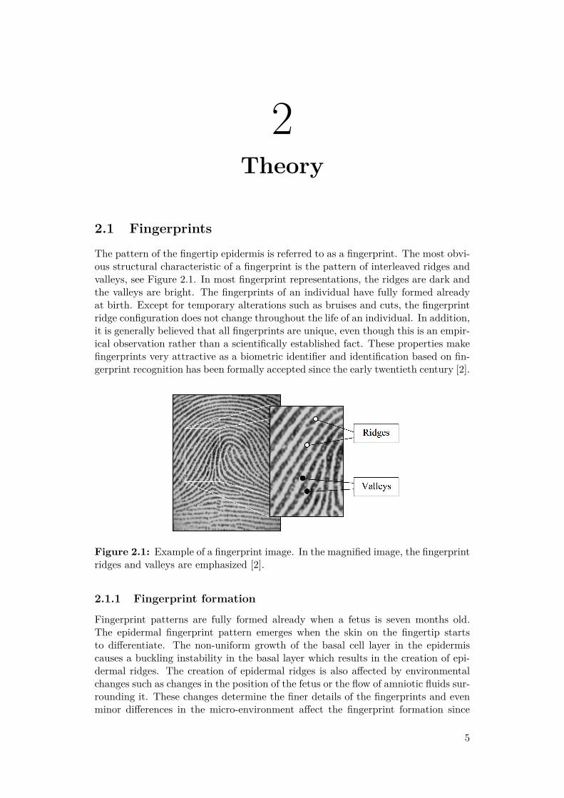
The pattern of the fingertip epidermis is referred to as a fingerprint. The most obvi-ous structural characteristic of a fingerprint is the pattern of interleaved ridges andvalleys, see Figure 2.1. In most fingerprint representations, the ridges are dark andthe valleys are bright. The fingerprints of an individual have fully formed alreadyat birth. Except for temporary alterations such as bruises and cuts, the fingerprintridge configuration does not change throughout the life of an individual. In addition,it is generally believed that all fingerprints are unique, even though this is an empir-ical observation rather than a scientifically established fact. These properties makefingerprints very attractive as a biometric identifier and identification based on fin-gerprint recognition has been formally accepted since the early twentieth century [2].

Figure 2.1: Example of a fingerprint image. In the magnified image, the fingerprintridges and valleys are emphasized [2].

2.1.1 Fingerprint formation

Fingerprint patterns are fully formed already when a fetus is seven months old.The epidermal fingerprint pattern emerges when the skin on the fingertip startsto differentiate. The non-uniform growth of the basal cell layer in the epidermiscauses a buckling instability in the basal layer which results in the creation of epi-dermal ridges. The creation of epidermal ridges is also affected by environmentalchanges such as changes in the position of the fetus or the flow of amniotic fluids sur-rounding it. These changes determine the finer details of the fingerprints and evenminor differences in the micro-environment affect the fingerprint formation since

5

2. Theory

the changes are amplified by the differentiation process of the cells. Also, since themicro-environment slightly differs from finger to finger, the cells will grow differ-ently on all fingers and thus the fingerprints of an individual will become uniqueeven though the genetic material influencing the differentiation process is identi-cal. The huge variety in environmental changes and genetic information makes itvirtually impossible for two fingers to get the exact same fingerprint pattern [2, 16].

2.1.2 Fingerprint representation

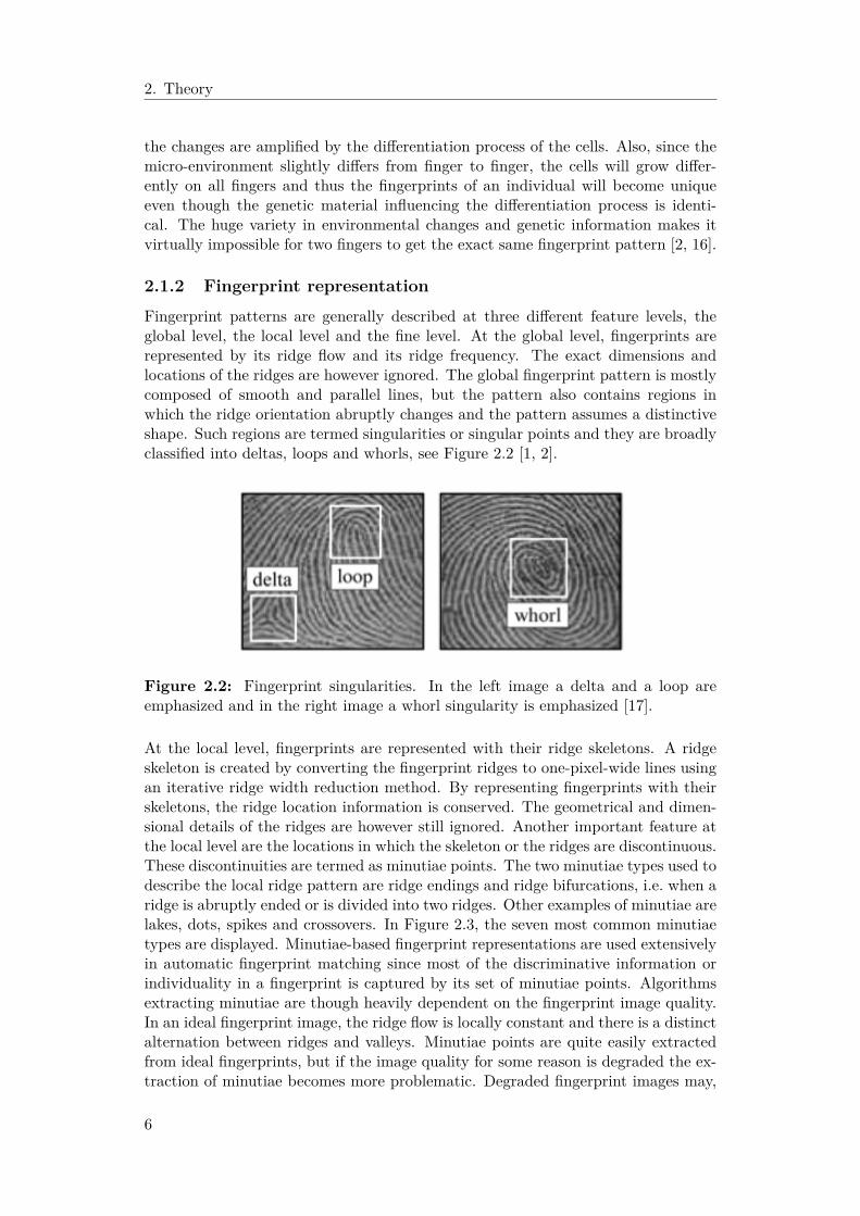
Fingerprint patterns are generally described at three different feature levels, theglobal level, the local level and the fine level. At the global level, fingerprints arerepresented by its ridge flow and its ridge frequency. The exact dimensions andlocations of the ridges are however ignored. The global fingerprint pattern is mostlycomposed of smooth and parallel lines, but the pattern also contains regions inwhich the ridge orientation abruptly changes and the pattern assumes a distinctiveshape. Such regions are termed singularities or singular points and they are broadlyclassified into deltas, loops and whorls, see Figure 2.2 [1, 2].

Figure 2.2: Fingerprint singularities. In the left image a delta and a loop areemphasized and in the right image a whorl singularity is emphasized [17].

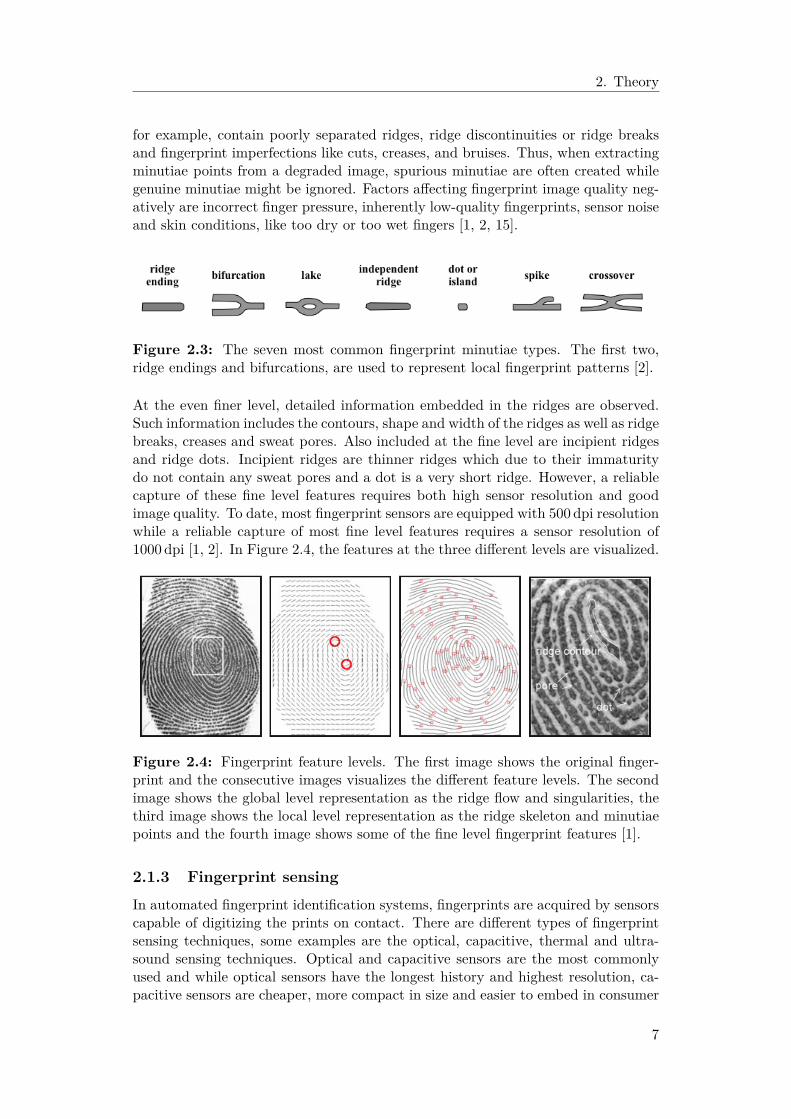
At the local level, fingerprints are represented with their ridge skeletons. A ridgeskeleton is created by converting the fingerprint ridges to one-pixel-wide lines usingan iterative ridge width reduction method. By representing fingerprints with theirskeletons, the ridge location information is conserved. The geometrical and dimen-sional details of the ridges are however still ignored. Another important feature atthe local level are the locations in which the skeleton or the ridges are discontinuous.These discontinuities are termed as minutiae points. The two minutiae types used todescribe the local ridge pattern are ridge endings and ridge bifurcations, i.e. when aridge is abruptly ended or is divided into two ridges. Other examples of minutiae arelakes, dots, spikes and crossovers. In Figure 2.3, the seven most common minutiaetypes are displayed. Minutiae-based fingerprint representations are used extensivelyin automatic fingerprint matching since most of the discriminative information orindividuality in a fingerprint is captured by its set of minutiae points. Algorithmsextracting minutiae are though heavily dependent on the fingerprint image quality.In an ideal fingerprint image, the ridge flow is locally constant and there is a distinctalternation between ridges and valleys. Minutiae points are quite easily extractedfrom ideal fingerprints, but if the image quality for some reason is degraded the ex-traction of minutiae becomes more problematic. Degraded fingerprint images may,

6

2. Theory

for example, contain poorly separated ridges, ridge discontinuities or ridge breaksand fingerprint imperfections like cuts, creases, and bruises. Thus, when extractingminutiae points from a degraded image, spurious minutiae are often created whilegenuine minutiae might be ignored. Factors affecting fingerprint image quality neg-atively are incorrect finger pressure, inherently low-quality fingerprints, sensor noiseand skin conditions, like too dry or too wet fingers [1, 2, 15].

Figure 2.3: The seven most common fingerprint minutiae types. The first two,ridge endings and bifurcations, are used to represent local fingerprint patterns [2].

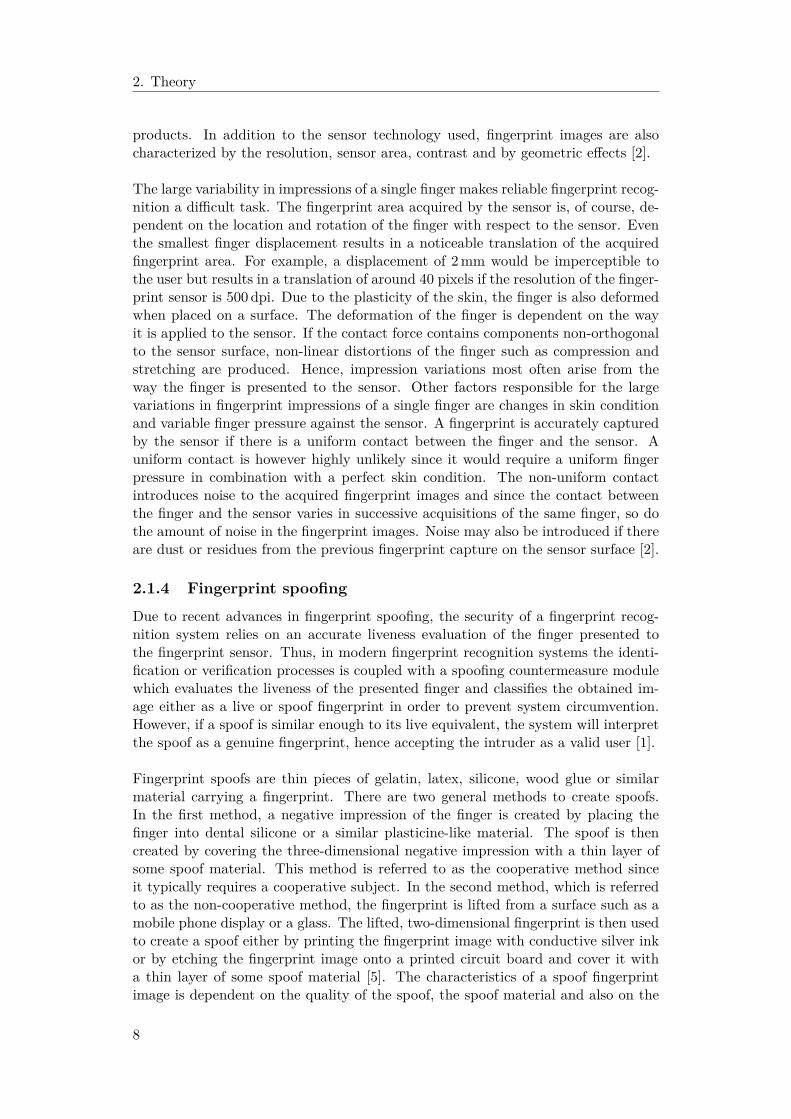
At the even finer level, detailed information embedded in the ridges are observed.Such information includes the contours, shape and width of the ridges as well as ridgebreaks, creases and sweat pores. Also included at the fine level are incipient ridgesand ridge dots. Incipient ridges are thinner ridges which due to their immaturitydo not contain any sweat pores and a dot is a very short ridge. However, a reliablecapture of these fine level features requires both high sensor resolution and goodimage quality. To date, most fingerprint sensors are equipped with 500 dpi resolutionwhile a reliable capture of most fine level features requires a sensor resolution of1000 dpi [1, 2]. In Figure 2.4, the features at the three different levels are visualized.

Figure 2.4: Fingerprint feature levels. The first image shows the original finger-print and the consecutive images visualizes the different feature levels. The secondimage shows the global level representation as the ridge flow and singularities, thethird image shows the local level representation as the ridge skeleton and minutiaepoints and the fourth image shows some of the fine level fingerprint features [1].

2.1.3 Fingerprint sensing

In automated fingerprint identification systems, fingerprints are acquired by sensorscapable of digitizing the prints on contact. There are different types of fingerprintsensing techniques, some examples are the optical, capacitive, thermal and ultra-sound sensing techniques. Optical and capacitive sensors are the most commonlyused and while optical sensors have the longest history and highest resolution, ca-pacitive sensors are cheaper, more compact in size and easier to embed in consumer

7

2. Theory

products. In addition to the sensor technology used, fingerprint images are alsocharacterized by the resolution, sensor area, contrast and by geometric effects [2].

The large variability in impressions of a single finger makes reliable fingerprint recog-nition a difficult task. The fingerprint area acquired by the sensor is, of course, de-pendent on the location and rotation of the finger with respect to the sensor. Eventhe smallest finger displacement results in a noticeable translation of the acquiredfingerprint area. For example, a displacement of 2 mm would be imperceptible tothe user but results in a translation of around 40 pixels if the resolution of the finger-print sensor is 500 dpi. Due to the plasticity of the skin, the finger is also deformedwhen placed on a surface. The deformation of the finger is dependent on the wayit is applied to the sensor. If the contact force contains components non-orthogonalto the sensor surface, non-linear distortions of the finger such as compression andstretching are produced. Hence, impression variations most often arise from theway the finger is presented to the sensor. Other factors responsible for the largevariations in fingerprint impressions of a single finger are changes in skin conditionand variable finger pressure against the sensor. A fingerprint is accurately capturedby the sensor if there is a uniform contact between the finger and the sensor. Auniform contact is however highly unlikely since it would require a uniform fingerpressure in combination with a perfect skin condition. The non-uniform contactintroduces noise to the acquired fingerprint images and since the contact betweenthe finger and the sensor varies in successive acquisitions of the same finger, so dothe amount of noise in the fingerprint images. Noise may also be introduced if thereare dust or residues from the previous fingerprint capture on the sensor surface [2].

2.1.4 Fingerprint spoofing

Due to recent advances in fingerprint spoofing, the security of a fingerprint recog-nition system relies on an accurate liveness evaluation of the finger presented tothe fingerprint sensor. Thus, in modern fingerprint recognition systems the identi-fication or verification processes is coupled with a spoofing countermeasure modulewhich evaluates the liveness of the presented finger and classifies the obtained im-age either as a live or spoof fingerprint in order to prevent system circumvention.However, if a spoof is similar enough to its live equivalent, the system will interpretthe spoof as a genuine fingerprint, hence accepting the intruder as a valid user [1].

Fingerprint spoofs are thin pieces of gelatin, latex, silicone, wood glue or similarmaterial carrying a fingerprint. There are two general methods to create spoofs.In the first method, a negative impression of the finger is created by placing thefinger into dental silicone or a similar plasticine-like material. The spoof is thencreated by covering the three-dimensional negative impression with a thin layer ofsome spoof material. This method is referred to as the cooperative method sinceit typically requires a cooperative subject. In the second method, which is referredto as the non-cooperative method, the fingerprint is lifted from a surface such as amobile phone display or a glass. The lifted, two-dimensional fingerprint is then usedto create a spoof either by printing the fingerprint image with conductive silver inkor by etching the fingerprint image onto a printed circuit board and cover it witha thin layer of some spoof material [5]. The characteristics of a spoof fingerprintimage is dependent on the quality of the spoof, the spoof material and also on the

8

2. Theory

fingerprint sensor since the material properties of the different spoof materials arenot equally compatible with the different sensor technologies.

2.2 Fingerprint image pre-processingIn the following sections, some background and theory related to the feature designpart of the thesis are presented. Subjects included are fingerprint image segmenta-tion, fingerprint pattern orientation, fingerprint image binarization, morphologicaloperations used to analyze the fingerprint patterns as well as minutiae extraction.

2.2.1 Segmentation

If the finger is not in contact with the entire sensor area when the fingerprint imageis captured, the resulting image will also contain some background. For sensorswhich create images in which the ridges are dark and the valleys are bright, theimage background will also be bright since no signal is generated in the non-contactarea. The process in which a fingerprint image is separated into foreground andbackground is referred to as fingerprint segmentation. The fingerprint area of theimage, which is characterized by the striped and oriented ridge and valley pattern,is denoted foreground and the bright area caused by deficient finger presentationis denoted background. By separating the foreground from the background, theanalysis of the fingerprint image can be constrained to the relevant area of the fin-gerprint image. A segmentation algorithm can be used to assign each pixel in animage to either the foreground or the background. The output of such an algorithmis a binary map of the same size as the image in which the pixels belonging to theforeground are ones and the pixels belonging to the background are zeros [2].

The segmentation algorithm implemented in this thesis is based on three pixel fea-tures; local gradient coherence, local intensity mean and local intensity variance.Due to lack of signal in the background, the local mean intensity is generally higherin the background than in the foreground. The intensity variance is high in theforeground due to the ridge and valley pattern, whereas only a small variance dueto noise is seen in the background. There can however be some darker clusters inthe background due to dust or grease on the fingerprint sensor, hence an additionalfeature is needed to make the segmentation algorithm robust to noise. Gradientcoherence is a pixel feature which can discriminate the oriented pattern in the fore-ground from the isotropic pattern in the background. It measures to which degreethe squared gradient vectors in a neighborhood share orientation. The gradientcoherence is one if all the squared gradient vectors in a neighborhood are paralleland the gradient coherence is zero if the squared gradient vectors are equally dis-tributed over all directions. Since a fingerprint consists of parallel line structures,the squared gradients in a neighborhood is more likely to point in the same direc-tion in the foreground. The squared gradients in the background should to a largerextent be equally distributed due to noise and lack of parallel line structures [2, 18].

2.2.2 Fingerprint orientation

The tangential direction of the ridge or valley lines passing through a pixel is referredto as the ridge or fingerprint orientation at the given pixel. The orientation of a

9

2. Theory

fingerprint image describes the coarse structure of the fingerprint pattern. Theorientation map, which also is referred to as the directional field, of a fingerprintimage is a matrix of the same size as the fingerprint image in which each matrixelement contains the orientation of the corresponding pixel in the fingerprint image.In principle, the directional field in a fingerprint image is perpendicular to the angleof the local gradients in the image. Thus, the directional field is often estimatedby averaging the gradients in a local neighborhood. However, since the anglesof the gradients in an image range between 0 and 2π and the orientation onlyrange between 0 and π, a traditional averaging of the gradients in a neighborhoodis not applicable. This is because gradient vectors pointing in opposite directionscancel each other out in a conventional averaging operation, although these oppositepointing gradient vectors imply the same fingerprint orientation. This problem isoften solved by doubling the angles of the gradient vectors before performing theaveraging. The cyclic properties of the angles result in orientation angles in therange 0 and π when the doubled angles later are converted back. The length ofthe gradient vector is often also considered when estimating the orientation in animage by allowing the angles of the steeper gradients in a neighborhood to affectthe orientation estimation more than the angles of the less steep gradients [1, 19].

2.2.3 Binarization

Binarization is the process in which an intensity image is converted to a binary im-age by grouping all the pixel values in an image into two modes. The two modes areseparated by assigning the pixels above a certain intensity threshold to the imageforeground and by assigning the pixels below the threshold to the image background.The intensity threshold is either determined on a global or a local scale and while aglobal threshold is constant and applicable to the entire image, a local threshold maydiffer in different parts of the image. A global threshold is often determined usingan approach referred to as Otsu’s method. Otsu’s method calculates the optimumglobal threshold of an image by maximizing the inter-class variance and minimizingthe intra-class variance with respect to the intensity values in the two modes. Alocal threshold is instead based on properties of a neighborhood, for example, theaverage pixel intensity in the neighborhood [20].

The success of an intensity-based thresholding is directly related to the intensityvalues in the image or in the local neighborhood. If the intensity histogram ofthe area of interest contains two well separated peaks, the chance of a successfulseparation of the modes in this area is high. However, if the histogram peaks arepoorly separated or if the peaks are too wide, the selection of a threshold whichwould result in a successful separation of the modes becomes more problematic [20].

2.2.4 Morphological operations

Mathematical morphology is a technique based on set theory, lattice theory andintegral geometry which is used in the analysis and processing of spatial structures.By applying morphological operations to an image, structures in the image may beextracted or modified. The most fundamental morphological operators are dilationand erosion. Other important concepts in morphology are opening, closing and theextraction of connected components and image skeletons. When processing an im-

10

2. Theory

age with a morphological operator, the image is probed with a structuring elementwhich is a small set of pixels. The structuring element is shifted over the entireimage and in each pixel, the properties of interest in the morphological operation isevaluated. Properties of interest might for example be the union or the intersectionof the structuring element and the underlying image pixels [20, 21].

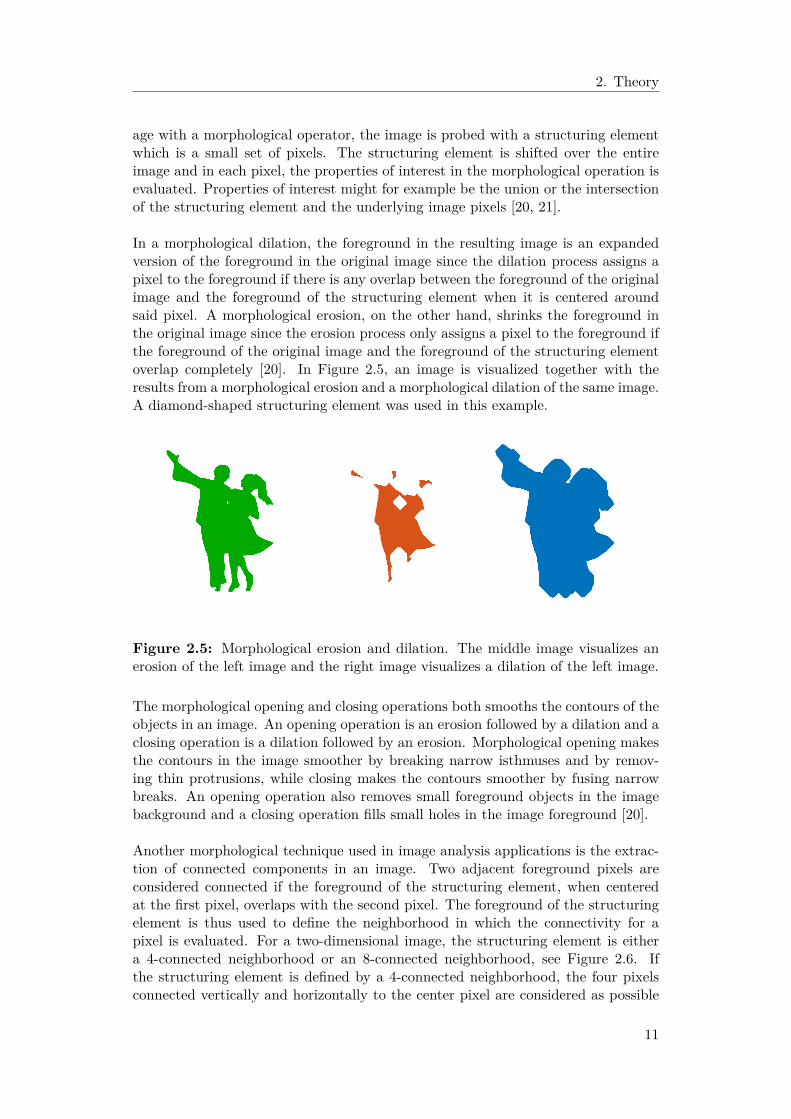
In a morphological dilation, the foreground in the resulting image is an expandedversion of the foreground in the original image since the dilation process assigns apixel to the foreground if there is any overlap between the foreground of the originalimage and the foreground of the structuring element when it is centered aroundsaid pixel. A morphological erosion, on the other hand, shrinks the foreground inthe original image since the erosion process only assigns a pixel to the foreground ifthe foreground of the original image and the foreground of the structuring elementoverlap completely [20]. In Figure 2.5, an image is visualized together with theresults from a morphological erosion and a morphological dilation of the same image.A diamond-shaped structuring element was used in this example.

Figure 2.5: Morphological erosion and dilation. The middle image visualizes anerosion of the left image and the right image visualizes a dilation of the left image.

The morphological opening and closing operations both smooths the contours of theobjects in an image. An opening operation is an erosion followed by a dilation and aclosing operation is a dilation followed by an erosion. Morphological opening makesthe contours in the image smoother by breaking narrow isthmuses and by remov-ing thin protrusions, while closing makes the contours smoother by fusing narrowbreaks. An opening operation also removes small foreground objects in the imagebackground and a closing operation fills small holes in the image foreground [20].

Another morphological technique used in image analysis applications is the extrac-tion of connected components in an image. Two adjacent foreground pixels areconsidered connected if the foreground of the structuring element, when centeredat the first pixel, overlaps with the second pixel. The foreground of the structuringelement is thus used to define the neighborhood in which the connectivity for apixel is evaluated. For a two-dimensional image, the structuring element is eithera 4-connected neighborhood or an 8-connected neighborhood, see Figure 2.6. Ifthe structuring element is defined by a 4-connected neighborhood, the four pixelsconnected vertically and horizontally to the center pixel are considered as possible

11

2. Theory

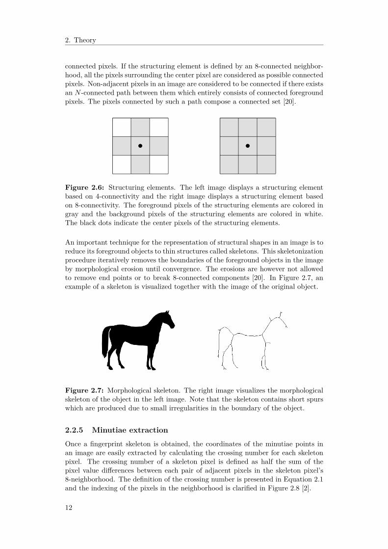
connected pixels. If the structuring element is defined by an 8-connected neighbor-hood, all the pixels surrounding the center pixel are considered as possible connectedpixels. Non-adjacent pixels in an image are considered to be connected if there existsan N -connected path between them which entirely consists of connected foregroundpixels. The pixels connected by such a path compose a connected set [20].

Figure 2.6: Structuring elements. The left image displays a structuring elementbased on 4-connectivity and the right image displays a structuring element basedon 8-connectivity. The foreground pixels of the structuring elements are colored ingray and the background pixels of the structuring elements are colored in white.The black dots indicate the center pixels of the structuring elements.

An important technique for the representation of structural shapes in an image is toreduce its foreground objects to thin structures called skeletons. This skeletonizationprocedure iteratively removes the boundaries of the foreground objects in the imageby morphological erosion until convergence. The erosions are however not allowedto remove end points or to break 8-connected components [20]. In Figure 2.7, anexample of a skeleton is visualized together with the image of the original object.

Figure 2.7: Morphological skeleton. The right image visualizes the morphologicalskeleton of the object in the left image. Note that the skeleton contains short spurswhich are produced due to small irregularities in the boundary of the object.

2.2.5 Minutiae extraction

Once a fingerprint skeleton is obtained, the coordinates of the minutiae points inan image are easily extracted by calculating the crossing number for each skeletonpixel. The crossing number of a skeleton pixel is defined as half the sum of thepixel value differences between each pair of adjacent pixels in the skeleton pixel’s8-neighborhood. The definition of the crossing number is presented in Equation 2.1and the indexing of the pixels in the neighborhood is clarified in Figure 2.8 [2].

12

2. Theory

crossing number = 0.57∑

i=0| Pi+1 mod 8 − Pi | (2.1)

Figure 2.8: Crossing number neighborhood. This is a schematic view of the neigh-borhood indexing around a skeleton pixel when its crossing number is calculated.

The crossing number is zero for isolated dots in the skeleton, one for skeleton endpoints, two for intermediate skeleton points, three for skeleton bifurcations and fourfor skeleton crossovers [2]. In Figure 2.9, examples of skeleton neighborhoods forthree of these minutiae types are visualized. The crossing number of the centerpixels in these examples are calculated from the pixels inside the marked areas.

Figure 2.9: Examples of minutiae points neighborhoods. The center pixel in theleft neighborhood is a skeleton bifurcation, the center pixel in the middle neighbor-hood is a skeleton end point and the center pixel in the right neighborhood is askeleton crossover. The skeleton foreground pixels are the pixels in black.

2.3 Learning-based feature extractionThis section presents some background to learning-based tools for feature extrac-tion, that is, neural networks and more specifically convolutional neural networks.

In recent years, deep learning and neural networks has come to provide powerfulsolutions to complex computer vision tasks such as recognition and classification.Deep learning refers to a machine learning technique in which deep network struc-tures automatically learn appropriate internal representations, i.e. features, of theobserved data and neural networks are such learnable network structures which areinspired by the human brain and its neural pathways. Convolutional neural net-works are a specialized form of neural networks in which at least one of the networklayers utilizes convolutional operations (i.e. filtering) [22].

13

2. Theory

A typical convolutional neural network consists of three types of layers; convolu-tional layers, pooling layers and fully connected layers. In a convolutional layer,convolutional operations are performed on the input to produce a set of linear ac-tivations, or feature maps, which are processed by non-linear activation functionssuch as the rectified linear unit function. Since each convolutional layer consists ofseveral filters which extract different features, several feature maps are produced ineach convolutional layer. While the first convolutional layers in the network typi-cally identify edges, corners and extended contours, the higher level convolutionallayers in the network structure encode more abstract features. Pooling layers in thenetwork modifies the output from the previous convolutional layer by aggregatingthe activation information of neighboring pixels. The pooling operations often re-duce the size of the feature maps by replacing each of the sets of neighboring pixelsin the input feature map with a single pixel value representing the neighborhoodstatistics. The max pooling operation, which passes the maximum activation valuein each neighborhood, is the most commonly used pooling operation. The poolingoperations in the network structure produce feature maps which are less sensitive tolocal translations in the input image, thus enabling extraction of features which aremore invariant of local translations in the original image higher up in the hierarchi-cal model. The last few layers in a convolutional network are fully connected layers,which means that all its neurons are directly connected to all the activations in theprevious layer. Such layers are computationally expensive but are needed at the endof the network to combine the final feature maps and to reach a final classificationdecision. The last fully connected layer is often followed by a softmax function inorder to convert the network output to posterior probabilities [22].

Convolutional neural networks are often trained by combining an optimization al-gorithm such as stochastic gradient descent with the back-propagation algorithm.A set of labelled images is needed to train the network and the general practice isto divide this set into a training set, a validation set and a test set. The trainingand validation sets are both used when training the network. The training set isused to calculate the gradients needed for updating the network parameters in theback-propagation, while the validation set is only used to monitor the training pro-cess. The training progress is evaluated after an epoch is completed, i.e. when theentire set of training images have been processed. During each epoch of training, theimages in the training set are further divided into smaller image sets called batches.The images in each batch are randomly fed through the network and by comparingthe actual network outputs with the desired network outputs the learning algorithmupdates the network parameters such that the discrepancies in the current batch areminimized. Once all the batches are processed, the next epoch is initiated [23, 24].

14

3Methods

In this chapter, the methods used in the thesis are presented. The chapter is dividedinto two sections. The first section presents the methods used in the feature designpart of the thesis and the second section presents the methods used in the learning-based liveness classification part of the thesis. The software used when implementingthe algorithms was MATLAB R2016b. In the second part of the thesis, the publiclyavailable MATLAB toolbox MatConvNet [25] was also used.

3.1 Feature design for fingerprint liveness classification

In the feature design part of the thesis, a data set provided by Fingerprint Cards wasused. The data set contained around 9000 images of live fingerprints and around12000 images of wood glue spoofs. The sensor used to acquire these images is thefingerprint touch sensor FPC1025, which is a capacitive sensor generating normal-ized images of size 160× 160 at a resolution of 508 dpi. The fingerprints in the liveimages originate from 240 unique fingers and the spoof images originate from thefake counterparts of these 240 fingers. Since the sensor used is significantly smallerthan a fingerprint, the data set contains several images of each finger as an attemptto capture the entire fingerprint in the data set. The data set also contained in-formation about pairs of images of the same fingerprints in which an overlap ofthe two prints has been established. The affine transformations needed to alignthe images in the pairs were also provided by Fingerprint Cards. There were 186image pairs in which a spoof image was found to overlap with a live image and 1266pairs of images in which two live images were found to overlap. The images in thefirst set of image pairs were used to identify and detect differences between live andspoof images and the images in the second set of image pairs were used as a reference.

The first step in the liveness feature design part of the thesis was to identify fea-tures which frequently differed between live and spoof images in the data set pro-vided by Fingerprint Cards. By registering, or aligning, the images in each imagepair containing one live image and one spoof image, the comparison was facilitated.During the visual inspection of the spoof images, the fingerprint valleys were foundto be more discontinuous in the spoof images than in the live images. Such dis-continuities result in spurious minutiae in the form of skeleton breaks, hence thesediscontinuities could be detected by analyzing the skeleton (see Section 3.1.6.1 forthis analysis). Another difference found was that the contours of the ridges andvalleys were somewhat more irregular in the spoof images than in the live images.Since irregular contours result in spurious minutiae in the form of spikes as well asin a more jagged skeleton, these can be captured by detecting spikes in the skele-

15

3. Methods

ton (Section 3.1.6.2) and by assessing the fingerprint skeleton curvature (Section3.1.6.3). During the visual inspection of the image pairs, some tendencies related tothe image intensity was also found. Thus, the intensities in the images were studied(Section 3.1.7.1). Included in these tendencies were that the ridges in the spooffingerprint images quite often were found to be more gray than the ridges in theirlive equivalents. The valley intensities in the spoof images did also often differ fromthe valleys in their live equivalents, but in an inconsistent manner, i.e. the valleyintensities in the spoof images were both brighter and darker than the valley inten-sities in the live fingerprint images. The spoof fabrication process is also believedto introduce a sharp shift between the ridges and valleys, hence the steepness of theintensity profile perpendicular to the ridge and valley pattern was assessed (Section3.1.7.2). The width of the ridges and valleys were also found to differ between thelive images and the spoof images. The width variations were investigated both byapplying a distance transform to the binarized fingerprint images (Section 3.1.8.1)and by measuring the relative width of the ridges and valleys in the image pairs(Section 3.1.8.2). Since the frequencies present in the image relates to the ridge andvalley width, the frequency content of the images was also studied (Section 3.1.8.3).The different parts of the analysis are explained in detail in the sections below.

3.1.1 Registration

The paired images were spatially aligned by transforming the coordinate system ofone of the images in the pair into the coordinate system of the other image in thepair. Apart from differences in translation and rotation, two images of the samefingerprint may also be somewhat scaled due to differences in pressure betweenthe finger and the sensor. Hence, an affine transformation is needed to align theimages. The affine transformations needed to align the images in the data set wereextracted from the matching algorithm used at Fingerprint Cards. In the image pairscontaining one spoof and one live image, the spoof images were used as targets andthe live images were used as source images. In the image pairs used as references,both the source and target images were images of live fingerprints. The images inthe pairs were aligned by transforming, i.e. warping, the source images according tothe affine transformations. The registration process is visualized in Figure 3.1.

Figure 3.1: Visualization of the registration process. The left image is a spoofimage used as target, the middle image is a live image used as source and the rightimage is the live image transformed to the coordinate system of the spoof image.

16

3. Methods

3.1.2 Visual interpretation

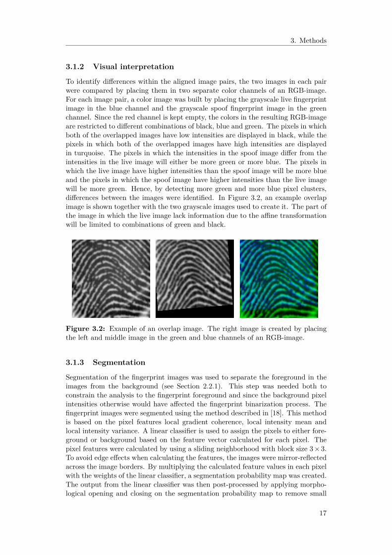
To identify differences within the aligned image pairs, the two images in each pairwere compared by placing them in two separate color channels of an RGB-image.For each image pair, a color image was built by placing the grayscale live fingerprintimage in the blue channel and the grayscale spoof fingerprint image in the greenchannel. Since the red channel is kept empty, the colors in the resulting RGB-imageare restricted to different combinations of black, blue and green. The pixels in whichboth of the overlapped images have low intensities are displayed in black, while thepixels in which both of the overlapped images have high intensities are displayedin turquoise. The pixels in which the intensities in the spoof image differ from theintensities in the live image will either be more green or more blue. The pixels inwhich the live image have higher intensities than the spoof image will be more blueand the pixels in which the spoof image have higher intensities than the live imagewill be more green. Hence, by detecting more green and more blue pixel clusters,differences between the images were identified. In Figure 3.2, an example overlapimage is shown together with the two grayscale images used to create it. The part ofthe image in which the live image lack information due to the affine transformationwill be limited to combinations of green and black.

Figure 3.2: Example of an overlap image. The right image is created by placingthe left and middle image in the green and blue channels of an RGB-image.

3.1.3 Segmentation

Segmentation of the fingerprint images was used to separate the foreground in theimages from the background (see Section 2.2.1). This step was needed both toconstrain the analysis to the fingerprint foreground and since the background pixelintensities otherwise would have affected the fingerprint binarization process. Thefingerprint images were segmented using the method described in [18]. This methodis based on the pixel features local gradient coherence, local intensity mean andlocal intensity variance. A linear classifier is used to assign the pixels to either fore-ground or background based on the feature vector calculated for each pixel. Thepixel features were calculated by using a sliding neighborhood with block size 3× 3.To avoid edge effects when calculating the features, the images were mirror-reflectedacross the image borders. By multiplying the calculated feature values in each pixelwith the weights of the linear classifier, a segmentation probability map was created.The output from the linear classifier was then post-processed by applying morpho-logical opening and closing on the segmentation probability map to remove small

17

3. Methods

clusters and holes in the map. The structuring elements used in the opening andclosing were disc-shaped elements. The diameter of the structuring element used inthe opening operation was 3 pixels, while the diameter of the structuring elementused in the closing operation was 5 pixels. In an additional post-processing step, allbackground clusters not connected to an image edge were discarded.

Segmentation masks were created for all the images analyzed in the liveness featuredesign part of the thesis. Since one of the images in each pair was transformedinto the coordinate system of the other image in the pair during the analysis, thecorresponding segmentation masks were transformed in the same manner. A jointsegmentation mask was then created for each image pair by calculating the intersec-tion of the aligned segmentation masks for each image pair. In order to avoid edgeeffects in the analysis of the images, reduced versions of the segmentation maskswere also created by filtering the joint masks with a minimum filter of size 7 × 7.Since zero-padding was used during filtering, this operation removed a three-pixelwide segment around the entire foreground of each mask.

The segmentation of the fingerprint images was evaluated both by manual inspectionand by calculating the Dice similarity coefficient for fingerprint images segmentedwith the implemented algorithm and the gold standard, which in this case are fin-gerprint images that are segmented manually. The Dice coefficient is a commonlyused measure to evaluate the similarity between image sets and it is defined byEquation 3.1. This coefficient ranges between zero and one and a Dice coefficientof zero indicates that there is no similarity between the two images while a Dicecoefficient of one indicates that the two images are identical. In Equation 3.1, Xand Y corresponds to automatic and manual (i.e. gold standard) segmentations.

Dice coefficient = 2|X ∩ Y ||X|+ |Y | (3.1)

The gold standard used when calculating the Dice coefficient was obtained by man-ually labelling 30 fingerprint images in the data set. All 30 images contained reason-ably large background areas and none of them belonged to any of the image pairsused in the feature design analysis.

3.1.4 Fingerprint orientation

The orientation in the fingerprint images (see Section 2.2.2) was estimated by im-plementing the method proposed in [19]. In this method, the directional field isestimated by calculating the dominant gradient direction in the neighborhood sur-rounding each pixel. Since the directional field is perpendicular to the dominantgradient direction, the conversion between the two is trivial. The implemented al-gorithm followed the general concepts of this method, but some alterations weremade to the proposed filtering steps. First, the gradients in each image were ob-tained by filtering the fingerprint images with a Gaussian derivative filter of size 7×7with standard deviation 1. The principal gradient directions were then estimatedby applying Principal Component Analysis (PCA) to the covariance matrix of thegradient components as proposed in [19]. The traditional averaging proposed for

18

3. Methods

this step was however replaced with a smoothing operation using a Gaussian filterof size 19× 19 with standard deviation 3. The components of the directional vectorfield were then calculated and after an additional smoothing of the vector field com-ponents, again using a Gaussian filter of size 19× 19 with standard deviation 3, thedominant gradient directions was calculated from the smoothed vector components.Finally, the fingerprint orientation was calculated by adding π/2 to the dominantgradient direction estimations in each pixel since the orientation and the dominantgradient direction are orthogonal.

3.1.5 Fingerprint binarization

The fingerprint images were converted to binary images by replacing all pixel valuesabove an image specific threshold with ones and by replacing all the other pixelvalues with zeros. The thresholds were calculated using Otsu’s method (see Section2.2.3) in order to maximize the inter-class variations between the ridges and valleysin each image. Only the values of the pixels assigned to the image foreground in thesegmentation process were used to calculate the thresholds. A global threshold waspreferred over a local threshold since local thresholds may introduce artifacts to thebinary images. Since the fingerprint valleys are the brighter pixels in the fingerprintpattern, the foreground of the resulting binary image mostly contained fingerprintvalleys. The complement of each image was also produced in order to obtain imagesin which the foreground contained the ridges of the fingerprint patterns.

3.1.6 Fingerprint skeletons

Fingerprint skeletons were produced by performing a morphological skeletonizationof the binary fingerprint images (see Section 2.2.4). Ridge skeletons were producedfrom the binary images in which the foreground consisted of ridges and valley skele-tons were produced from the binary images in which the foreground consisted ofvalleys. In order to constrain the analysis of the images in an image pair to thesame part of the fingerprint, the skeleton foreground pixels which coincided withbackground pixels of their joint segmentation mask were converted to the skeletonimage background.

3.1.6.1 Detection of skeleton breaks

Breaks in the fingerprint skeletons were detected by identifying end points in theskeleton and by finding pairs of end points in close proximity to each other. Thenumber of skeleton breaks in the ridge skeletons and the valley skeletons were calcu-lated for both images in each image pair. The end points in an image were identifiedby finding the pixels with crossing number one. Isolated islands in the skeletons werealso considered as end points, hence the pixels for which the crossing number waszero were also considered as end points. Any end points outside the foreground ofthe corresponding joint and reduced segmentation mask were however ignored inorder to avoid detection of false skeleton end points. All pairs of end points whichwere closer than 20 pixels apart were considered as possible skeleton breaks. Thenumber of possible breaks in an image was then narrowed down by removing allpairs of end points which were connected by the skeleton. In order to prevent im-proper break detections due to incorrect fingerprint orientation estimations like the

19

3. Methods

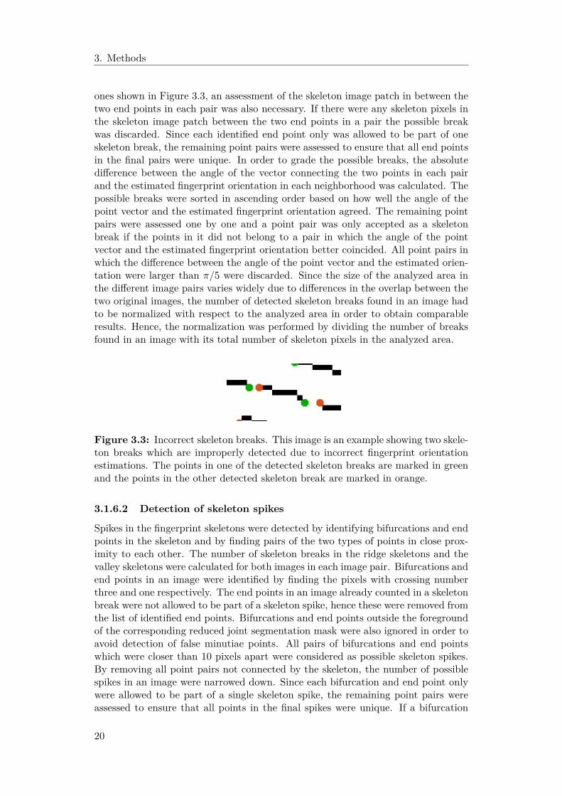
ones shown in Figure 3.3, an assessment of the skeleton image patch in between thetwo end points in each pair was also necessary. If there were any skeleton pixels inthe skeleton image patch between the two end points in a pair the possible breakwas discarded. Since each identified end point only was allowed to be part of oneskeleton break, the remaining point pairs were assessed to ensure that all end pointsin the final pairs were unique. In order to grade the possible breaks, the absolutedifference between the angle of the vector connecting the two points in each pairand the estimated fingerprint orientation in each neighborhood was calculated. Thepossible breaks were sorted in ascending order based on how well the angle of thepoint vector and the estimated fingerprint orientation agreed. The remaining pointpairs were assessed one by one and a point pair was only accepted as a skeletonbreak if the points in it did not belong to a pair in which the angle of the pointvector and the estimated fingerprint orientation better coincided. All point pairs inwhich the difference between the angle of the point vector and the estimated orien-tation were larger than π/5 were discarded. Since the size of the analyzed area inthe different image pairs varies widely due to differences in the overlap between thetwo original images, the number of detected skeleton breaks found in an image hadto be normalized with respect to the analyzed area in order to obtain comparableresults. Hence, the normalization was performed by dividing the number of breaksfound in an image with its total number of skeleton pixels in the analyzed area.

Figure 3.3: Incorrect skeleton breaks. This image is an example showing two skele-ton breaks which are improperly detected due to incorrect fingerprint orientationestimations. The points in one of the detected skeleton breaks are marked in greenand the points in the other detected skeleton break are marked in orange.

3.1.6.2 Detection of skeleton spikes

Spikes in the fingerprint skeletons were detected by identifying bifurcations and endpoints in the skeleton and by finding pairs of the two types of points in close prox-imity to each other. The number of skeleton breaks in the ridge skeletons and thevalley skeletons were calculated for both images in each image pair. Bifurcations andend points in an image were identified by finding the pixels with crossing numberthree and one respectively. The end points in an image already counted in a skeletonbreak were not allowed to be part of a skeleton spike, hence these were removed fromthe list of identified end points. Bifurcations and end points outside the foregroundof the corresponding reduced joint segmentation mask were also ignored in order toavoid detection of false minutiae points. All pairs of bifurcations and end pointswhich were closer than 10 pixels apart were considered as possible skeleton spikes.By removing all point pairs not connected by the skeleton, the number of possiblespikes in an image were narrowed down. Since each bifurcation and end point onlywere allowed to be part of a single skeleton spike, the remaining point pairs wereassessed to ensure that all points in the final spikes were unique. If a bifurcation

20

3. Methods

was connected to more than one end point, the pair with the shortest Euclideandistance between the points was considered as most probable to be a skeleton spike.Just as when grading the possible skeleton breaks, the possible spikes were gradedby calculating the absolute difference between the angle of the vector connecting thetwo points in each pair and the estimated fingerprint orientation in each neighbor-hood. However, since the angle between the bifurcation and the end point defininga skeleton spike should be somewhat orthogonal, the possible spikes were sorted inascending order based on how close the difference between vector angle and esti-mated neighborhood orientation came to π/2. The remaining point pairs were thenassessed one by one and a point pair was only accepted as a skeleton spike if thepoints in it were not already part of a pair in which the angle of the point vectorand the estimated orientation better coincided with π/2. All point pairs in whichthe difference between the angle of the point vector and the estimated fingerprintorientation were further away than π/5 from π/2 were discarded. Since the numberof skeleton bifurcations also was found to be a feature which differed between liveskeletons and spoof skeletons, the number of detected bifurcations in a fingerprintskeleton that were not already part of a detected spike was also saved for each image.Both the number of detected spikes and the number of detected bifurcations in animage were normalized by dividing with its total number of skeleton pixels.

3.1.6.3 Skeleton curvature

The curvature of a two-dimensional curve is a measure of how sharply the curvebends. It is defined as the magnitude of the rate of change of the unit tangentvector with respect to the curve length. The curvature at a point on a parametriccurve given by (x(s), y(s)) is often calculated from the first and second derivativesof the curve at the point with respect to the parameter s using Equation 3.2 [26].

κ = | x′y′′ − y′x′′ |(x′ 2 + y′ 2 ) 2/3 (3.2)

If a curve is discrete, as in the segments of a fingerprint skeleton, a slight modifica-tion of the curvature definition is needed to compensate for sampling differences ofthe discrete points on the curve. In order to calculate the curvature at a point ona discrete curve, the relative positions of its predecessor and successor are needed.The derivatives in Equation 3.2 are first calculated by fitting the three sequentialpoints to two polynomials and then the curvature at the points is estimated [26, 27].

The jaggedness of a fingerprint skeleton was evaluated by estimating the mean cur-vature for all its curve segments. The skeleton curvature was calculated for bothimages in each image pair. As in the previous sections, the analysis of the finger-print skeletons of an image pair was constrained to the pixels corresponding to theforeground area of the joint segmentation mask. Since the curvature at skeletonbifurcations and skeleton crossovers would shadow the smaller curvature variationsoriginating from skeleton jaggedness, the skeleton pixels in a patch of size 3 × 3around each bifurcation and crossover were removed from the skeleton before thecurve segments were extracted from the skeleton image. Groups of connected pixelswere extracted by identifying all 8-connections in the skeleton. The curvature wascalculated for each curve segment of connected skeleton pixels containing at least

21

3. Methods

three connected pixels. The absolute curvature values in all the points along eachcurve segment were summed up and divided by the number of estimated curvaturevalues in the same segment. At last, a measure of the curvature in an entire fin-gerprint skeleton was obtained by taking the mean of the curvature values of all itsskeleton curve segments.

3.1.7 Fingerprint intensities

The intensity of the fingerprint images was studied in three different ways. Theintensity distributions of the fingerprint images were studied both by evaluating allintensity values in the ridges and valleys and by evaluating the image intensity valuesin the pixels along the fingerprint skeletons. Since the spoof fabrication process isbelieved to introduce a sharper shift between the ridges and valleys, the steepness ofthe intensity profile perpendicular to the ridge and valley pattern was also assessed.

3.1.7.1 Intensity distributions

The intensity distribution analysis was performed both by calculating the meanof the intensities along the ridges and valleys in each fingerprint image and bycalculating the mean of the intensities along the ridge and valley skeletons of eachfingerprint image. The mean intensity values were calculated for both images ineach image pair and the analysis was constrained to the pixel values correspondingto the foreground area of the joint segmentation mask.

3.1.7.2 Intensity profiles

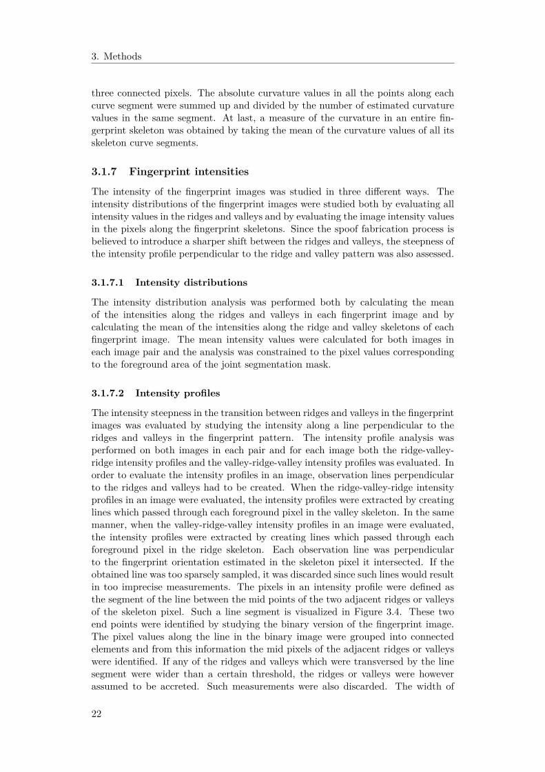
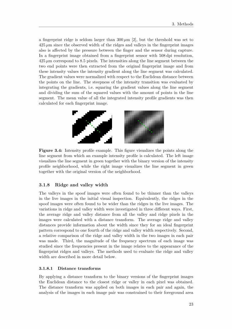
The intensity steepness in the transition between ridges and valleys in the fingerprintimages was evaluated by studying the intensity along a line perpendicular to theridges and valleys in the fingerprint pattern. The intensity profile analysis wasperformed on both images in each pair and for each image both the ridge-valley-ridge intensity profiles and the valley-ridge-valley intensity profiles was evaluated. Inorder to evaluate the intensity profiles in an image, observation lines perpendicularto the ridges and valleys had to be created. When the ridge-valley-ridge intensityprofiles in an image were evaluated, the intensity profiles were extracted by creatinglines which passed through each foreground pixel in the valley skeleton. In the samemanner, when the valley-ridge-valley intensity profiles in an image were evaluated,the intensity profiles were extracted by creating lines which passed through eachforeground pixel in the ridge skeleton. Each observation line was perpendicularto the fingerprint orientation estimated in the skeleton pixel it intersected. If theobtained line was too sparsely sampled, it was discarded since such lines would resultin too imprecise measurements. The pixels in an intensity profile were defined asthe segment of the line between the mid points of the two adjacent ridges or valleysof the skeleton pixel. Such a line segment is visualized in Figure 3.4. These twoend points were identified by studying the binary version of the fingerprint image.The pixel values along the line in the binary image were grouped into connectedelements and from this information the mid pixels of the adjacent ridges or valleyswere identified. If any of the ridges and valleys which were transversed by the linesegment were wider than a certain threshold, the ridges or valleys were howeverassumed to be accreted. Such measurements were also discarded. The width of

22

3. Methods

a fingerprint ridge is seldom larger than 300µm [2], but the threshold was set to425µm since the observed width of the ridges and valleys in the fingerprint imagesalso is affected by the pressure between the finger and the sensor during capture.In a fingerprint image obtained from a fingerprint sensor with 508 dpi resolution,425µm correspond to 8.5 pixels. The intensities along the line segment between thetwo end points were then extracted from the original fingerprint image and fromthese intensity values the intensity gradient along the line segment was calculated.The gradient values were normalized with respect to the Euclidean distance betweenthe points on the line. The steepness of the intensity transition was evaluated byintegrating the gradients, i.e. squaring the gradient values along the line segmentand dividing the sum of the squared values with the amount of points in the linesegment. The mean value of all the integrated intensity profile gradients was thencalculated for each fingerprint image.

Figure 3.4: Intensity profile example. This figure visualizes the points along theline segment from which an example intensity profile is calculated. The left imagevisualizes the line segment in green together with the binary version of the intensityprofile neighborhood, while the right image visualizes the line segment in greentogether with the original version of the neighborhood.

3.1.8 Ridge and valley width

The valleys in the spoof images were often found to be thinner than the valleysin the live images in the initial visual inspection. Equivalently, the ridges in thespoof images were often found to be wider than the ridges in the live images. Thevariations in ridge and valley width were investigated in three different ways. First,the average ridge and valley distance from all the valley and ridge pixels in theimages were calculated with a distance transform. The average ridge and valleydistances provide information about the width since they for an ideal fingerprintpattern correspond to one fourth of the ridge and valley width respectively. Second,a relative comparison of the ridge and valley width in the two images in each pairwas made. Third, the magnitude of the frequency spectrum of each image wasstudied since the frequencies present in the image relates to the appearance of thefingerprint ridges and valleys. The methods used to evaluate the ridge and valleywidth are described in more detail below.

3.1.8.1 Distance transforms

By applying a distance transform to the binary versions of the fingerprint imagesthe Euclidean distance to the closest ridge or valley in each pixel was obtained.The distance transform was applied on both images in each pair and again, theanalysis of the images in each image pair was constrained to their foreground area

23

3. Methods

of the joint segmentation mask. A distance transform of a binary image returns adistance map in which the value of each pixel corresponds to the distance to theclosest foreground pixel in the image. Hence, the distance to the closest ridge foreach valley pixel in an image was evaluated by applying the distance transform tothe binary image in which the ridges belong to the foreground. Conversely, thedistance to the closest valley for each ridge pixel in an image was evaluated byapplying the distance transform to the binary image in which the valleys belong tothe foreground. The average distance to the closest ridge in all the valley pixels ineach image and the average distance to the closest valley in all the ridge pixels in animage was then calculated. Distances exceeding a certain threshold, which was setslightly higher than half the largest acceptable ridge and valley width (4.25 pixels),were however discarded before the averaging since such measurements originatedfrom areas in the fingerprint images where the ridges or valleys in the binary imageswere not represented correctly.

3.1.8.2 Relative ridge and valley width

The relative width of the ridges and valleys in an image pair was estimated bypairwise comparisons of the ridge and valley widths. For each image pair, theoverlapping foreground pixels in their skeletons determined the locations for whichthe width was assessed in. The ridge skeletons were used to find joint skeletonpixels to assess the ridge width in and the valley skeletons were used to find jointskeleton pixels to assess the valley width in. In order to evaluate the ridge or valleywidth in these joint pixels, lines which passed through each joint skeleton pixel withan angle perpendicular to the fingerprint orientation estimated in the same pixelswere created. By extracting the values of the line pixels from the correspondingbinary images and by grouping these values into connected components, the firstand last line pixel within the current ridge or valley was identified. The Euclideandistance between these two pixels on the line was calculated and then the ratiobetween the distances calculated for the same skeleton pixel in the two images of animage pair was determined. If an estimated ridge or valley width was wider than acertain threshold (set to 8.5 pixels), the measurement was however discarded sincethe ridge or valley then was assumed to be accreted with adjacent ridges or valleys.Other constraints put on the measurements were that the angles of the two linesintersecting the same joint skeleton pixel in an image pair were not allowed to differmore than π/12 and that the lines were not allowed to be too sparsely sampled.The relative width for each joint ridge skeleton pixel was calculated as the ratiobetween the estimated ridge width in the image used as target and the estimatedridge width in the warped image. The relative width for each joint valley skeletonpixel was calculated as the ratio between the estimated valley width in the warpedimage and the estimated valley width in the image used as target.

3.1.8.3 Frequency spectrum analysis

The frequency content of the fingerprint images was evaluated by studying the mag-nitude of their frequency spectra. The edge effects in the frequency spectra wereminimized by mirror reflecting the fingerprint images before converting them to thefrequency domain. In order to compare the frequency spectra of the live and spoofimages, the two-dimensional magnitudes of the frequency spectra were converted to a

24

3. Methods

one-dimensional signal representing the radial average of the frequency magnitudes.Since the one-dimensional signal is created by computing the frequency content av-erage along the radius, the frequency content in the corners of the frequency spectramagnitudes is ignored. The corners of the frequency spectra magnitudes for the fin-gerprint images do however only contain noise, thus no important information willbe lost in this conversion. The radial averages of the frequency spectra magnitudeswere calculated for all source and target images in the image pairs. An averageone-dimensional frequency spectrum magnitude signal was then calculated for allthe source and target fingerprint images for both the image pairs containing one liveand one spoof image and the image pairs in the reference data.

3.1.9 Statistical significance

The statistical significance of the detected features was evaluated by performingstatistical t-tests on the feature value distributions obtained for the image pairswhich contained both live and spoof fingerprint images. Paired-sample t-tests wereused for the skeleton-based features, the intensity distributions and the distributionsobtained from the distance transform analyses, while a two-sample t-test was usedfor the relative ridge and valley width analyses. All distributions were assumed to benormal distributions, but no assumptions regarding the variances were made. Thesignificance level used was 1% for all the features except for the relative valley widthwhere a significance level of 2.5% was used instead. The higher significance level wasused since the relative valley width result was not significant at the 1% significancelevel. One sided t-tests were used in most cases, but since the obtained resultsfor the skeleton curvature and the intensity profile analyses were opposite to theexpected, the significance of the difference between the live and spoof distributionsfrom these analyses was evaluated with a two-sided t-test. The null hypothesis inthe t-tests was that the mean of the spoof distribution equals the mean of the livedistribution. The alternative hypothesis in the one-sided t-tests was that the meanof the spoof distribution was greater than the mean of the live distribution. Theseshypotheses are specified in Equation 3.3. The difference between the distributionswas only considered significant if the null hypothesis could be rejected.

H0 : µspoof = µlive

H1 : µspoof > µlive

(3.3)

3.1.10 Spoof image quality

The quality of the spoof images was estimated using a binary support vector ma-chine model in which ten of the designed liveness features were used as predictors.These predictors were chosen by manually identifying the ten features which bestseparated the investigated live and spoof images. Features which did not show astatistically significant difference between the live and spoof images were not consid-ered to be relevant to include in the quality assessment model. The features chosenas predictors in the model are given in the list below. The fact that some of thesefeatures were correlated was ignored when they were selected as model predictors.

• breaks in the valley skeleton• spikes in the ridge skeleton

25

3. Methods

• spikes in the valley skeleton• bifurcations in the ridge skeleton• bifurcations in the valley skeleton• ridge skeleton curvature• ridge skeleton intensity• valley-ridge-valley intensity profiles• ridge-valley-ridge intensity profiles• distance to the closest valley

The binary support vector machine model aims to find a hyperplane that successfullyseparates the ten-dimensional predictor vectors in an optimal sense. The hyperplaneequation is given by Equation 3.4. In this equation, f(x) is the classification score, xis the feature vector consisting of the chosen predictors, β is a vector containing themodel weights and b is a bias term. The separating hyperplane corresponds to thefeature vector which satisfies f(x) = 0. A feature vector is classified as belonging toone of the two classes depending on the sign of its classification score, i.e. f(x) > 0implies a live classification and f(x) < 0 implies a spoof classification.

f(x) = x′β + b (3.4)

The support vector machine model was trained on the standardized feature vectorsobtained for all the images used for feature design (i.e. the pairs containing bothlive and spoof images) in order to obtain the separating hyperplane which best sep-arated the live and spoof images based on the ten predictors. When the model wasestimated, the spoof images in the set were classified with the model. The relativequality of the spoof images was then estimated from their classification scores. Thesupport vector machine classification score is defined as the signed distance fromthe decision boundary of the separating hyperplane. These scores were mapped intoposterior probabilities by an optimal score-to-posterior-probability transformationfunction. For inseparable classes, as in this case, this transformation is a sigmoidfunction. The quality of a spoof image is regarded as high if the posterior proba-bility of the live class is high and the quality of a spoof image is regarded as low ifthe posterior probability of the spoof class is high. The quality of an entire set ofspoof images may be defined as the percentage of these images that the separatinghyperplane model manages to classify correctly. The separating hyperplane modelcould of course also estimate the quality of the live images in a similar manner, butsuch an evaluation is outside the scope of this thesis.

3.2 Learning-based fingerprint liveness classificationIn the second part of the thesis, convolutional neural networks for fingerprint live-ness detection was implemented since the spoof quality in a data set also can beestimated from how well a state-of-the-art fingerprint liveness classifier performs onthe spoof images in the set. A set of fingerprint images is considered to be very hardto classify if the state-of-the-art network cannot differentiate between the live andfake images in the set. Conversely, if a shallow network easily differentiates spoofimages from live images, these images are considered easy to classify.

26

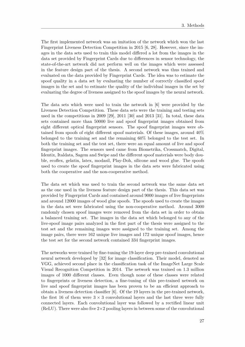
3. Methods

The first implemented network was an imitation of the network which won the lastFingerprint Liveness Detection Competition in 2015 [6, 28]. However, since the im-ages in the data sets used to train this model differed a lot from the images in thedata set provided by Fingerprint Cards due to differences in sensor technology, thestate-of-the-art network did not perform well on the images which were assessedin the feature design part of the thesis. A second network was thus trained andevaluated on the data provided by Fingerprint Cards. The idea was to estimate thespoof quality in a data set by evaluating the number of correctly classified spoofimages in the set and to estimate the quality of the individual images in the set byevaluating the degree of liveness assigned to the spoof images by the neural network.

The data sets which were used to train the network in [6] were provided by theLiveness Detection Competition. These data sets were the training and testing setsused in the competitions in 2009 [29], 2011 [30] and 2013 [31]. In total, these datasets contained more than 50000 live and spoof fingerprint images obtained fromeight different optical fingerprint sensors. The spoof fingerprint images were ob-tained from spoofs of eight different spoof materials. Of these images, around 40%belonged to the training set and the remaining 60% belonged to the test set. Inboth the training set and the test set, there were an equal amount of live and spooffingerprint images. The sensors used came from Biometrika, Crossmatch, Digital,Identix, Italdata, Sagem and Swipe and the different spoof materials were body dou-ble, ecoflex, gelatin, latex, modasil, Play-Doh, silicone and wood glue. The spoofsused to create the spoof fingerprint images in the data sets were fabricated usingboth the cooperative and the non-cooperative method.

The data set which was used to train the second network was the same data setas the one used in the liveness feature design part of the thesis. This data set wasprovided by Fingerprint Cards and contained around 9000 images of live fingerprintsand around 12000 images of wood glue spoofs. The spoofs used to create the imagesin the data set were fabricated using the non-cooperative method. Around 3000randomly chosen spoof images were removed from the data set in order to obtaina balanced training set. The images in the data set which belonged to any of thelive-spoof image pairs analyzed in the first part of the thesis were assigned to thetest set and the remaining images were assigned to the training set. Among theimage pairs, there were 162 unique live images and 172 unique spoof images, hencethe test set for the second network contained 334 fingerprint images.

The networks were trained by fine-tuning the 19-layer deep pre-trained convolutionalneural network developed by [32] for image classification. Their model, denoted asVGG, achieved second place in the classification task of the ImageNet Large ScaleVisual Recognition Competition in 2014. The network was trained on 1.3 millionimages of 1000 different classes. Even though none of these classes were relatedto fingerprints or liveness detection, a fine-tuning of this pre-trained network onlive and spoof fingerprint images has been proven to be an efficient approach toobtain a liveness detection classifier [6]. Of the 19 layers in the pre-trained network,the first 16 of them were 3 × 3 convolutional layers and the last three were fullyconnected layers. Each convolutional layer was followed by a rectified linear unit(ReLU). There were also five 2×2 pooling layers in between some of the convolutional

27

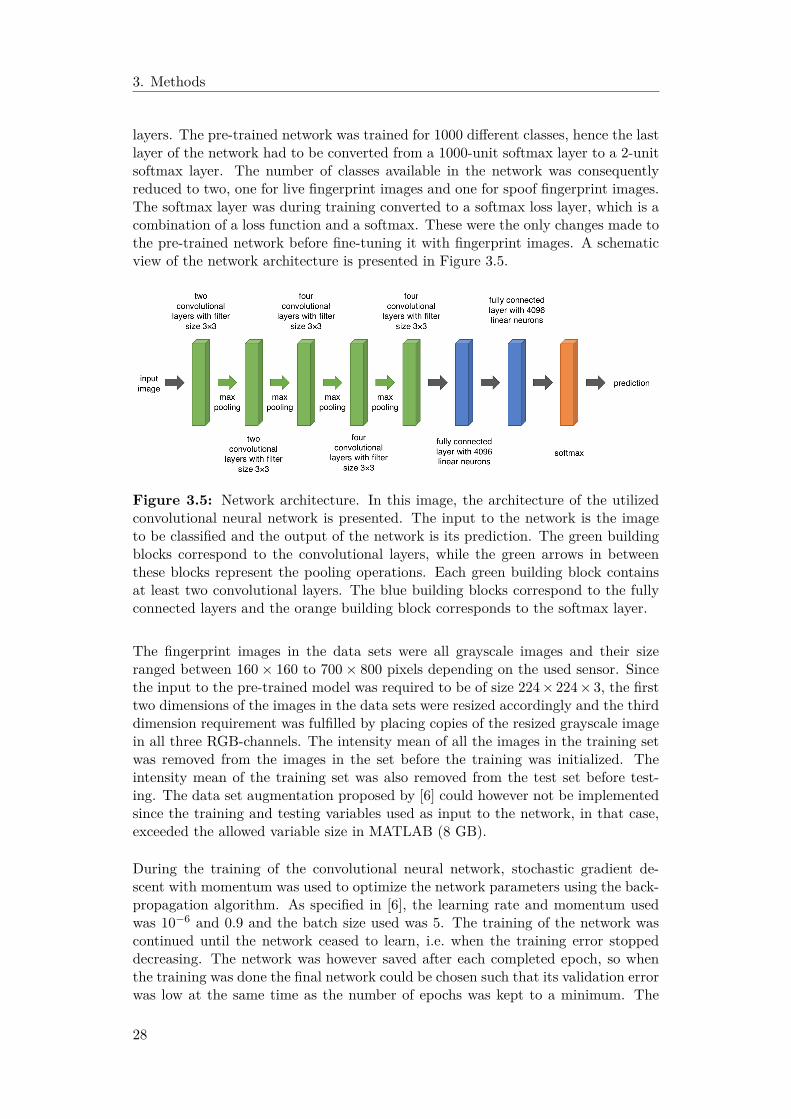
3. Methods

layers. The pre-trained network was trained for 1000 different classes, hence the lastlayer of the network had to be converted from a 1000-unit softmax layer to a 2-unitsoftmax layer. The number of classes available in the network was consequentlyreduced to two, one for live fingerprint images and one for spoof fingerprint images.The softmax layer was during training converted to a softmax loss layer, which is acombination of a loss function and a softmax. These were the only changes made tothe pre-trained network before fine-tuning it with fingerprint images. A schematicview of the network architecture is presented in Figure 3.5.

Figure 3.5: Network architecture. In this image, the architecture of the utilizedconvolutional neural network is presented. The input to the network is the imageto be classified and the output of the network is its prediction. The green buildingblocks correspond to the convolutional layers, while the green arrows in betweenthese blocks represent the pooling operations. Each green building block containsat least two convolutional layers. The blue building blocks correspond to the fullyconnected layers and the orange building block corresponds to the softmax layer.

The fingerprint images in the data sets were all grayscale images and their sizeranged between 160× 160 to 700× 800 pixels depending on the used sensor. Sincethe input to the pre-trained model was required to be of size 224× 224× 3, the firsttwo dimensions of the images in the data sets were resized accordingly and the thirddimension requirement was fulfilled by placing copies of the resized grayscale imagein all three RGB-channels. The intensity mean of all the images in the training setwas removed from the images in the set before the training was initialized. Theintensity mean of the training set was also removed from the test set before test-ing. The data set augmentation proposed by [6] could however not be implementedsince the training and testing variables used as input to the network, in that case,exceeded the allowed variable size in MATLAB (8 GB).

During the training of the convolutional neural network, stochastic gradient de-scent with momentum was used to optimize the network parameters using the back-propagation algorithm. As specified in [6], the learning rate and momentum usedwas 10−6 and 0.9 and the batch size used was 5. The training of the network wascontinued until the network ceased to learn, i.e. when the training error stoppeddecreasing. The network was however saved after each completed epoch, so whenthe training was done the final network could be chosen such that its validation errorwas low at the same time as the number of epochs was kept to a minimum. The

28

3. Methods

training of the first network was ran for 35 epochs and the final network was thenetwork obtained after 30 epochs. The training of the second network was ran for15 epochs and the final network was the network obtained after 11 epochs. Whenthe final network was identified, the network performance was evaluated on the testset. The classification performance of the obtained networks was evaluated by cal-culating the spoof false positive rate (SFPR), the spoof false negative rate (SFNR)and the average classification error (ACE) of the test sets. The spoof false positiverate is defined as the percentage of misclassified live images, the spoof false nega-tive rate is defined as the percentage of misclassified spoof images and the averageclassification error is defined as the average of the two.

29

3. Methods

30

4Experimental results and

analysis

4.1 Feature design for fingerprint liveness classificationIn the following sections, the experimental results of the liveness feature designpart of the thesis are presented and analyzed. In the first section below, a visualmotivation of the performed analyses is presented. This section is followed by asection in which the segmentation results are presented and by the sections in whichthe results from the designed fingerprint liveness features are presented.

4.1.1 Visual interpretation

During the visual inspection of the pairs of live and spoof fingerprint images, severaldetectable features were identified. Some of these features can be seen in the threeoverlap images presented in Figure 4.1. The most frequent feature found was valleydiscontinuities in the spoof images. This feature can be seen as blue interruptionsof the turquoise valleys in all three images in Figure 4.1. By studying these images,it can also be seen that the ridge and valley edges in the spoof images are somewhatmore irregular than the ridge and valley edges in the live images.

Figure 4.1: Visualization result examples. The overlap images from three imagepairs are presented in order to visualize some of the features detected when com-paring images obtained from live fingers and images obtained from spoofs. Recallthat blue and green colors originate from the live and spoof images respectively.

Some tendencies regarding the fingerprint image intensities were also noticed. Sincethe ridge color in the overlap images often was a mixture of black and green, theridges in the spoof fingerprint images were, in general, brighter than the ridges inthe live fingerprint images. The color of the valleys in the overlap images was quiteoften a more blue shade of turquoise which implied that the valley intensity in the

31

4. Experimental results and analysis

spoof images often was lower than the valley intensity in the live images. The green-ish ridge color can be seen in all three images in Figure 4.1, while the bluer shadeof turquoise is especially apparent in the right image.

Thinner valleys, or equivalently wider ridges, in the spoof images were another quitefrequently observed feature in the image pairs. At first glance, the blue appearanceof the valleys in the left image in Figure 4.1 might seem only to be due to a significantdifference in valley intensities between the live and the spoof image. However, froma closer inspection of Figure 4.2, in which this overlap image is displayed againtogether with the live and spoof images used to create it, it becomes clear that theblue appearance of the valleys in the overlap image is mostly due to the significantdifference in valley width between the live image and the spoof image, even thoughthere are intensity differences which also affect the appearance.

Figure 4.2: Visualization of an image pair in which there is a significant differencein ridge and valley width between the spoof image and the live image. The leftimage is the spoof image, the middle image is the live image and the right image isthe overlap image created from the two.

4.1.2 Segmentation

This section presents the results of the fingerprint segmentation. In Figure 4.3, threeexample segmentation results are presented by displaying the fingerprint imagestogether with the foreground borders in the corresponding segmentation masks.The Dice coefficient calculated for the test set containing 30 images ranged between0.9763 and 0.9995 and the mean Dice coefficient for the set was 0.9921.

Figure 4.3: Segmentation result examples. Three fingerprint images are displayedtogether with green lines representing the borders of their segmentation masks.

32

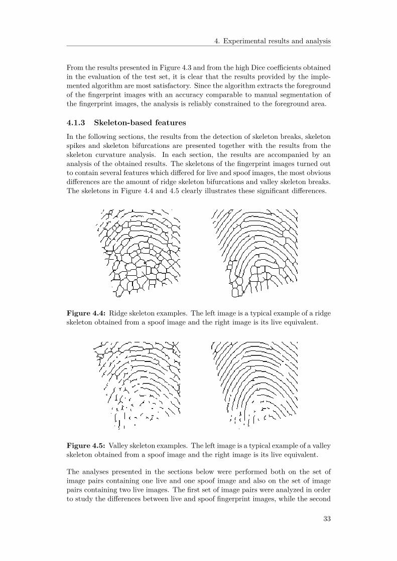
4. Experimental results and analysis

From the results presented in Figure 4.3 and from the high Dice coefficients obtainedin the evaluation of the test set, it is clear that the results provided by the imple-mented algorithm are most satisfactory. Since the algorithm extracts the foregroundof the fingerprint images with an accuracy comparable to manual segmentation ofthe fingerprint images, the analysis is reliably constrained to the foreground area.

4.1.3 Skeleton-based features

In the following sections, the results from the detection of skeleton breaks, skeletonspikes and skeleton bifurcations are presented together with the results from theskeleton curvature analysis. In each section, the results are accompanied by ananalysis of the obtained results. The skeletons of the fingerprint images turned outto contain several features which differed for live and spoof images, the most obviousdifferences are the amount of ridge skeleton bifurcations and valley skeleton breaks.The skeletons in Figure 4.4 and 4.5 clearly illustrates these significant differences.

Figure 4.4: Ridge skeleton examples. The left image is a typical example of a ridgeskeleton obtained from a spoof image and the right image is its live equivalent.

Figure 4.5: Valley skeleton examples. The left image is a typical example of a valleyskeleton obtained from a spoof image and the right image is its live equivalent.

The analyses presented in the sections below were performed both on the set ofimage pairs containing one live and one spoof image and also on the set of imagepairs containing two live images. The first set of image pairs were analyzed in orderto study the differences between live and spoof fingerprint images, while the second

33

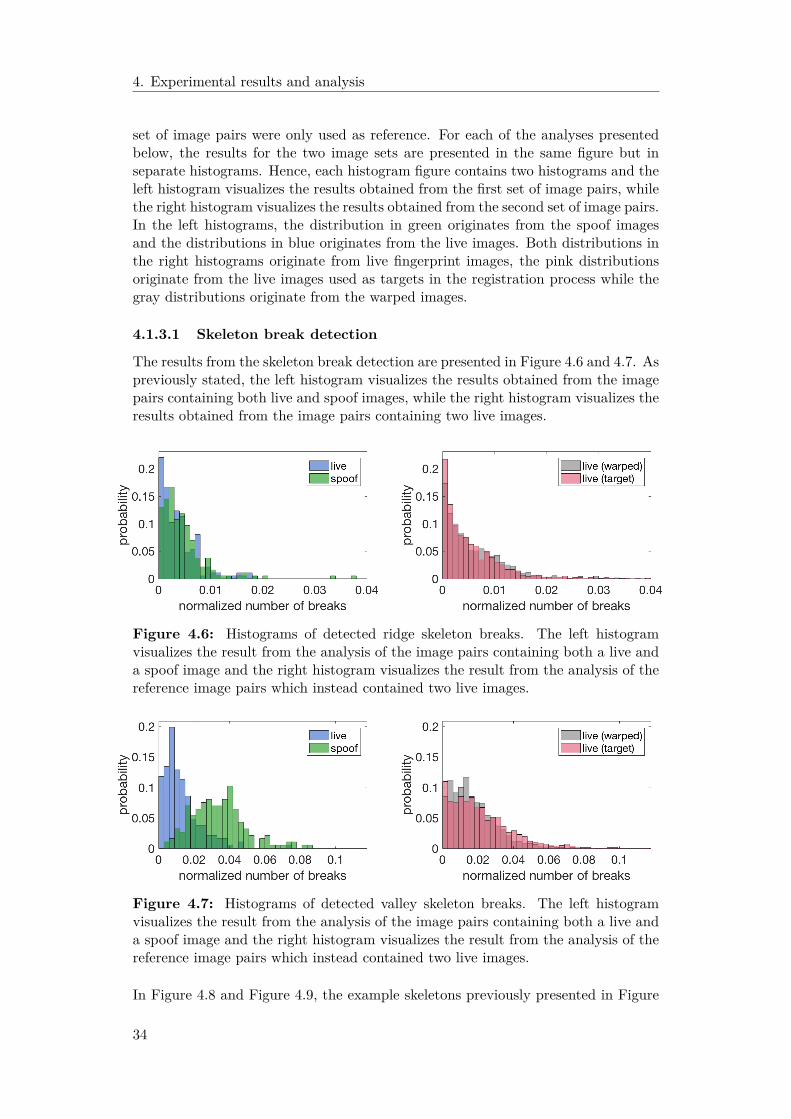
4. Experimental results and analysis

set of image pairs were only used as reference. For each of the analyses presentedbelow, the results for the two image sets are presented in the same figure but inseparate histograms. Hence, each histogram figure contains two histograms and theleft histogram visualizes the results obtained from the first set of image pairs, whilethe right histogram visualizes the results obtained from the second set of image pairs.In the left histograms, the distribution in green originates from the spoof imagesand the distributions in blue originates from the live images. Both distributions inthe right histograms originate from live fingerprint images, the pink distributionsoriginate from the live images used as targets in the registration process while thegray distributions originate from the warped images.

4.1.3.1 Skeleton break detection

The results from the skeleton break detection are presented in Figure 4.6 and 4.7. Aspreviously stated, the left histogram visualizes the results obtained from the imagepairs containing both live and spoof images, while the right histogram visualizes theresults obtained from the image pairs containing two live images.

Figure 4.6: Histograms of detected ridge skeleton breaks. The left histogramvisualizes the result from the analysis of the image pairs containing both a live anda spoof image and the right histogram visualizes the result from the analysis of thereference image pairs which instead contained two live images.

Figure 4.7: Histograms of detected valley skeleton breaks. The left histogramvisualizes the result from the analysis of the image pairs containing both a live anda spoof image and the right histogram visualizes the result from the analysis of thereference image pairs which instead contained two live images.

In Figure 4.8 and Figure 4.9, the example skeletons previously presented in Figure

34

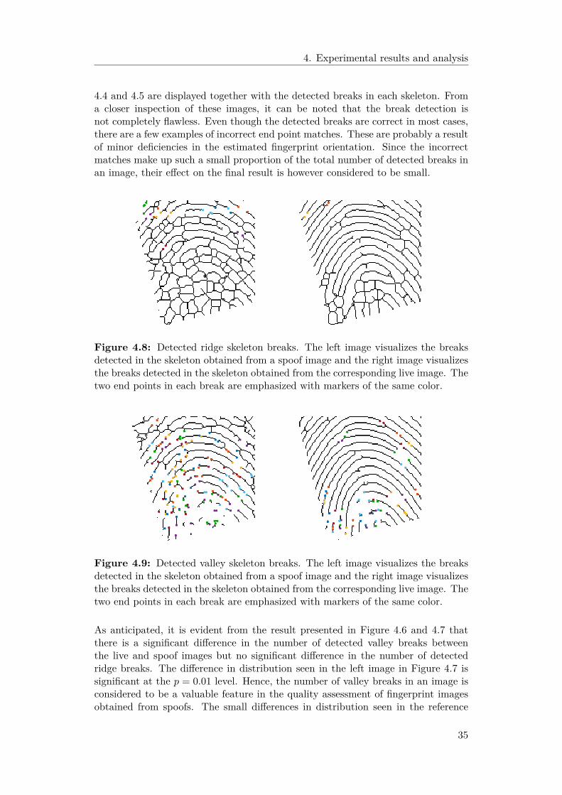
4. Experimental results and analysis

4.4 and 4.5 are displayed together with the detected breaks in each skeleton. Froma closer inspection of these images, it can be noted that the break detection isnot completely flawless. Even though the detected breaks are correct in most cases,there are a few examples of incorrect end point matches. These are probably a resultof minor deficiencies in the estimated fingerprint orientation. Since the incorrectmatches make up such a small proportion of the total number of detected breaks inan image, their effect on the final result is however considered to be small.

Figure 4.8: Detected ridge skeleton breaks. The left image visualizes the breaksdetected in the skeleton obtained from a spoof image and the right image visualizesthe breaks detected in the skeleton obtained from the corresponding live image. Thetwo end points in each break are emphasized with markers of the same color.

Figure 4.9: Detected valley skeleton breaks. The left image visualizes the breaksdetected in the skeleton obtained from a spoof image and the right image visualizesthe breaks detected in the skeleton obtained from the corresponding live image. Thetwo end points in each break are emphasized with markers of the same color.

As anticipated, it is evident from the result presented in Figure 4.6 and 4.7 thatthere is a significant difference in the number of detected valley breaks betweenthe live and spoof images but no significant difference in the number of detectedridge breaks. The difference in distribution seen in the left image in Figure 4.7 issignificant at the p = 0.01 level. Hence, the number of valley breaks in an image isconsidered to be a valuable feature in the quality assessment of fingerprint imagesobtained from spoofs. The small differences in distribution seen in the reference

35

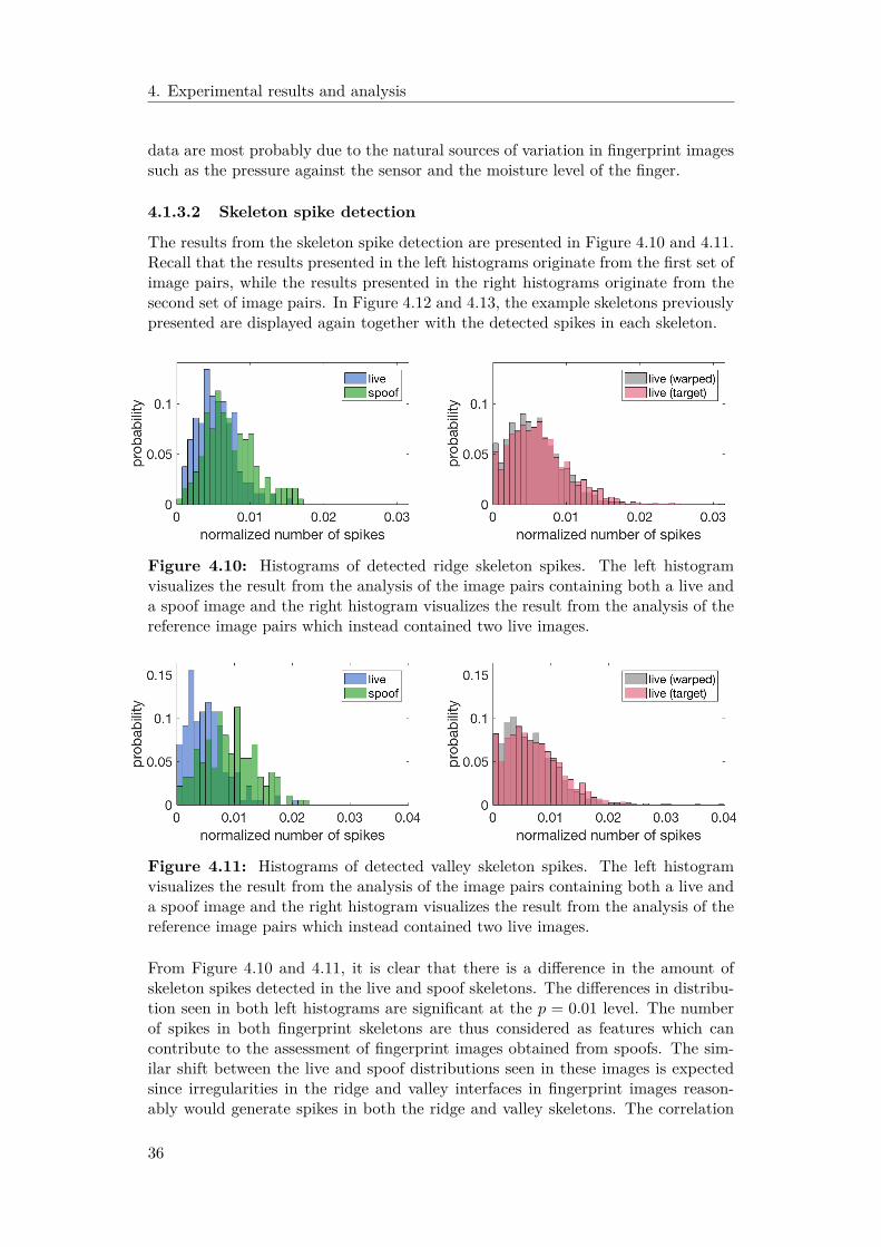
4. Experimental results and analysis

data are most probably due to the natural sources of variation in fingerprint imagessuch as the pressure against the sensor and the moisture level of the finger.

4.1.3.2 Skeleton spike detection

The results from the skeleton spike detection are presented in Figure 4.10 and 4.11.Recall that the results presented in the left histograms originate from the first set ofimage pairs, while the results presented in the right histograms originate from thesecond set of image pairs. In Figure 4.12 and 4.13, the example skeletons previouslypresented are displayed again together with the detected spikes in each skeleton.

Figure 4.10: Histograms of detected ridge skeleton spikes. The left histogramvisualizes the result from the analysis of the image pairs containing both a live anda spoof image and the right histogram visualizes the result from the analysis of thereference image pairs which instead contained two live images.

Figure 4.11: Histograms of detected valley skeleton spikes. The left histogramvisualizes the result from the analysis of the image pairs containing both a live anda spoof image and the right histogram visualizes the result from the analysis of thereference image pairs which instead contained two live images.

From Figure 4.10 and 4.11, it is clear that there is a difference in the amount ofskeleton spikes detected in the live and spoof skeletons. The differences in distribu-tion seen in both left histograms are significant at the p = 0.01 level. The numberof spikes in both fingerprint skeletons are thus considered as features which cancontribute to the assessment of fingerprint images obtained from spoofs. The sim-ilar shift between the live and spoof distributions seen in these images is expectedsince irregularities in the ridge and valley interfaces in fingerprint images reason-ably would generate spikes in both the ridge and valley skeletons. The correlation

36

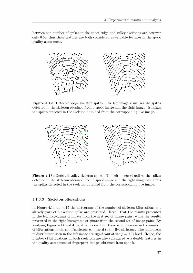
4. Experimental results and analysis

between the number of spikes in the spoof ridge and valley skeletons are howeveronly 0.52, thus these features are both considered as valuable features in the spoofquality assessment.

Figure 4.12: Detected ridge skeleton spikes. The left image visualizes the spikesdetected in the skeleton obtained from a spoof image and the right image visualizesthe spikes detected in the skeleton obtained from the corresponding live image.

Figure 4.13: Detected valley skeleton spikes. The left image visualizes the spikesdetected in the skeleton obtained from a spoof image and the right image visualizesthe spikes detected in the skeleton obtained from the corresponding live image.

4.1.3.3 Skeleton bifurcations

In Figure 4.14 and 4.15 the histograms of the number of skeleton bifurcations notalready part of a skeleton spike are presented. Recall that the results presentedin the left histograms originate from the first set of image pairs, while the resultspresented in the right histograms originate from the second set of image pairs. Bystudying Figure 4.14 and 4.15, it is evident that there is an increase in the numberof bifurcations in the spoof skeletons compared to the live skeletons. The differencesin distribution seen in the left image are significant at the p = 0.01 level. Hence, thenumber of bifurcations in both skeletons are also considered as valuable features inthe quality assessment of fingerprint images obtained from spoofs.

37

4. Experimental results and analysis

Figure 4.14: Histograms of the ridge skeleton bifurcations. The left histogramvisualizes the result from the analysis of the image pairs containing both a live anda spoof image and the right histogram visualizes the result from the analysis of thereference image pairs which instead contained two live images.

Figure 4.15: Histograms of the valley skeleton bifurcations. The left histogramvisualizes the result from the analysis of the image pairs containing both a live anda spoof image and the right histogram visualizes the result from the analysis of thereference image pairs which instead contained two live images.

The considerable shift in distribution seen in the left histogram in Figure 4.14 ismuch expected since an increased number of breaks in the valley skeleton impliesthat there is an increased number of bridges between adjacent ridges. Each bridgebetween adjacent ridges result in two additional bifurcations in the ridge skeleton,hence an increased number of breaks in the valley skeleton is analogous to an in-creased number of bifurcations in the ridge skeleton. The correlation between thenumber of breaks in the spoof valley skeletons and the number of bifurcations in thespoof ridge skeleton is 0.86, thus a combination of these two features in the qualityassessment of the fingerprint images will not yield an additive effect in the evaluationeven though both features are considered valuable. The shift in distribution seen inthe left histogram in Figure 4.15 is however not as expected. A possible explanationfor this might be that the skeletonization process tends to split ridge and valleyendings into two spikes. Since such spikes do not originate from irregular ridge andvalley edges, they should not be detected as spikes and hence the bifurcation in asplit ending is included in the bifurcation statistics. The correlation between thenumber of bifurcations in the valley skeleton and the number of end points in thevalley skeleton is however only 0.14, which suggests that the increased number ofbifurcations in the spoof valley skeletons is caused by other factors too.

38

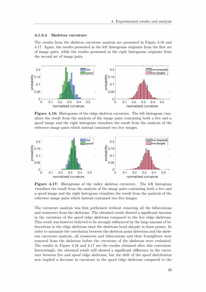
4. Experimental results and analysis

4.1.3.4 Skeleton curvature

The results from the skeleton curvature analysis are presented in Figure 4.16 and4.17. Again, the results presented in the left histograms originate from the first setof image pairs, while the results presented in the right histograms originate fromthe second set of image pairs.

Figure 4.16: Histograms of the ridge skeleton curvature. The left histogram visu-alizes the result from the analysis of the image pairs containing both a live and aspoof image and the right histogram visualizes the result from the analysis of thereference image pairs which instead contained two live images.

Figure 4.17: Histograms of the valley skeleton curvature. The left histogramvisualizes the result from the analysis of the image pairs containing both a live anda spoof image and the right histogram visualizes the result from the analysis of thereference image pairs which instead contained two live images.

The curvature analysis was first performed without removing all the bifurcationsand crossovers from the skeletons. The obtained result showed a significant increasein the curvature of the spoof ridge skeletons compared to the live ridge skeletons.This result was however believed to be strongly influenced by the large amount of bi-furcations in the ridge skeletons since the skeletons bend sharply in these points. Inorder to minimize the correlation between the skeleton point detection and the skele-ton curvature analysis, all crossovers and bifurcations and their 8-neighbors wereremoved from the skeletons before the curvature of the skeletons were evaluated.The results in Figure 4.16 and 4.17 are the results obtained after this correction.Interestingly, the obtained result still showed a significant difference in the curva-ture between live and spoof ridge skeletons, but the shift of the spoof distributionnow implied a decrease in curvature in the spoof ridge skeletons compared to the

39

4. Experimental results and analysis

live ridge skeletons. This result implies that the large amount of bifurcations andcrossovers removed from the ridge spoof skeletons actually did influence the previousresult strongly. A probable explanation for the significant decrease in curvature forthe spoof ridge skeletons is that their additional skeleton bifurcations and crossoversoften coincide with skeletons pixels in which the larger scale curvature is higher. Ifthis is the case, the curvature analysis might however not measure the jaggednessof the skeletons as intended, but instead measure the larger scale curvature of theridges and valleys. This explanation however still implies that the results are influ-enced by the amount of bifurcations in the spoof skeletons.

The difference in curvature between the live and spoof distributions in Figure 4.16is significant at the p = 0.01 level. The correlation between the number of detectedbifurcations and the skeleton curvature in the spoof ridge skeletons is −0.54. Theinfluence from the amount of detected skeleton bifurcations is thus considered not tobe large enough to exclude this feature from the final quality assessment model. Eventhough the curvature analysis probably did not manage to measure the jaggednessof the skeletons and instead is believed to measure the larger scale curvature of theridges and valleys, this feature is still considered valuable in the quality assessmentsince the larger scale curvature of the images in each pair should be the same.

4.1.4 Intensity distributions

In the following sections, the results from the intensity distribution analyses andthe intensity profile analysis are presented and discussed. These analyses were per-formed both on the set of image pairs containing one live and one spoof imageand also on the reference image pairs. For each of the analyses presented below,the results for the two image sets are presented in the same figure but in separatehistograms. Hence, each histogram figure contains two histograms and the left his-togram visualizes the results obtained from the first set of image pairs, while theright histogram visualizes the results obtained from the second set of image pairs.In the left histograms, the distribution in green originates from the spoof imagesand the distributions in blue originates from the live images. Both distributions inthe right histograms originate from live fingerprint images, the pink distributionsoriginate from the live images used as targets in the registration process while thegray distributions originate from the warped images.

4.1.4.1 Intensity distribution in fingerprint ridges and valleys

The results from the intensity distribution analysis of the ridges and valleys in thefingerprint images are presented in Figure 4.18 and 4.19. As previously stated, theleft histogram visualizes the results obtained from the image pairs containing bothlive and spoof fingerprint images, while the right histogram visualizes the resultsobtained from the image pairs containing two live fingerprint images.

As can be seen in Figure 4.18 and 4.19, no significant differences in the mean ridgeand valley intensity were found. This analysis relies heavily on the separation ofthe ridges and valleys in the binarization process. But since the binarization of theimages is based on global thresholds, the intensity variations in the ridges and valleysare naturally limited by the calculated thresholds. If the intensity in the ridges and

40

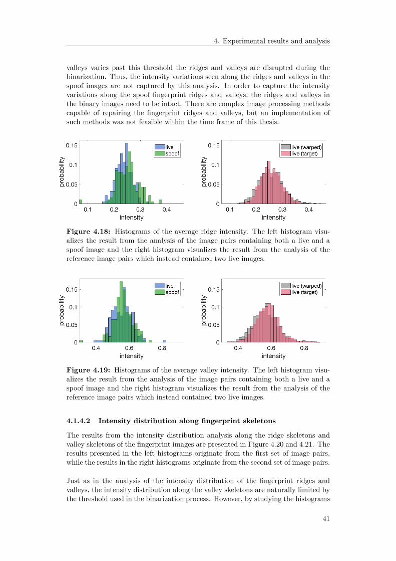
4. Experimental results and analysis

valleys varies past this threshold the ridges and valleys are disrupted during thebinarization. Thus, the intensity variations seen along the ridges and valleys in thespoof images are not captured by this analysis. In order to capture the intensityvariations along the spoof fingerprint ridges and valleys, the ridges and valleys inthe binary images need to be intact. There are complex image processing methodscapable of repairing the fingerprint ridges and valleys, but an implementation ofsuch methods was not feasible within the time frame of this thesis.

Figure 4.18: Histograms of the average ridge intensity. The left histogram visu-alizes the result from the analysis of the image pairs containing both a live and aspoof image and the right histogram visualizes the result from the analysis of thereference image pairs which instead contained two live images.

Figure 4.19: Histograms of the average valley intensity. The left histogram visu-alizes the result from the analysis of the image pairs containing both a live and aspoof image and the right histogram visualizes the result from the analysis of thereference image pairs which instead contained two live images.

4.1.4.2 Intensity distribution along fingerprint skeletons

The results from the intensity distribution analysis along the ridge skeletons andvalley skeletons of the fingerprint images are presented in Figure 4.20 and 4.21. Theresults presented in the left histograms originate from the first set of image pairs,while the results in the right histograms originate from the second set of image pairs.

Just as in the analysis of the intensity distribution of the fingerprint ridges andvalleys, the intensity distribution along the valley skeletons are naturally limited bythe threshold used in the binarization process. However, by studying the histograms

41

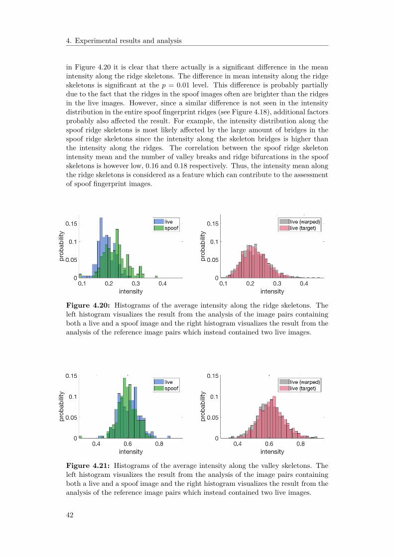
4. Experimental results and analysis

in Figure 4.20 it is clear that there actually is a significant difference in the meanintensity along the ridge skeletons. The difference in mean intensity along the ridgeskeletons is significant at the p = 0.01 level. This difference is probably partiallydue to the fact that the ridges in the spoof images often are brighter than the ridgesin the live images. However, since a similar difference is not seen in the intensitydistribution in the entire spoof fingerprint ridges (see Figure 4.18), additional factorsprobably also affected the result. For example, the intensity distribution along thespoof ridge skeletons is most likely affected by the large amount of bridges in thespoof ridge skeletons since the intensity along the skeleton bridges is higher thanthe intensity along the ridges. The correlation between the spoof ridge skeletonintensity mean and the number of valley breaks and ridge bifurcations in the spoofskeletons is however low, 0.16 and 0.18 respectively. Thus, the intensity mean alongthe ridge skeletons is considered as a feature which can contribute to the assessmentof spoof fingerprint images.

Figure 4.20: Histograms of the average intensity along the ridge skeletons. Theleft histogram visualizes the result from the analysis of the image pairs containingboth a live and a spoof image and the right histogram visualizes the result from theanalysis of the reference image pairs which instead contained two live images.

Figure 4.21: Histograms of the average intensity along the valley skeletons. Theleft histogram visualizes the result from the analysis of the image pairs containingboth a live and a spoof image and the right histogram visualizes the result from theanalysis of the reference image pairs which instead contained two live images.

42

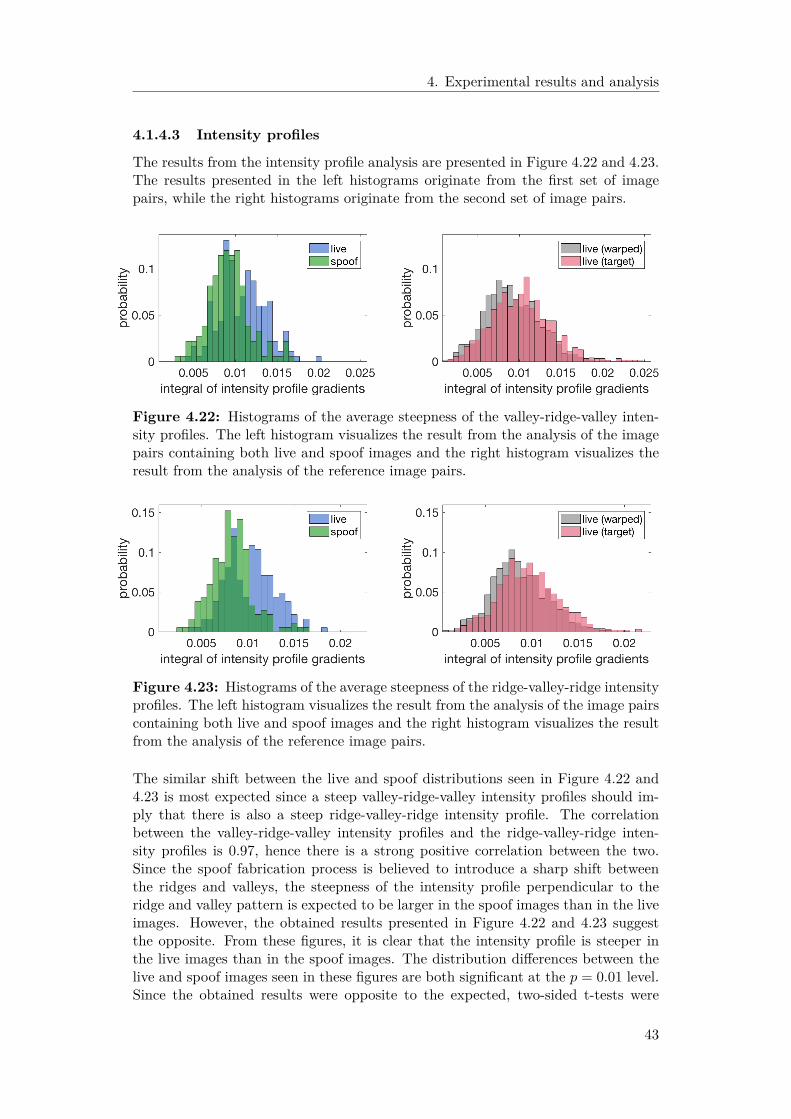
4. Experimental results and analysis

4.1.4.3 Intensity profiles

The results from the intensity profile analysis are presented in Figure 4.22 and 4.23.The results presented in the left histograms originate from the first set of imagepairs, while the right histograms originate from the second set of image pairs.

Figure 4.22: Histograms of the average steepness of the valley-ridge-valley inten-sity profiles. The left histogram visualizes the result from the analysis of the imagepairs containing both live and spoof images and the right histogram visualizes theresult from the analysis of the reference image pairs.

Figure 4.23: Histograms of the average steepness of the ridge-valley-ridge intensityprofiles. The left histogram visualizes the result from the analysis of the image pairscontaining both live and spoof images and the right histogram visualizes the resultfrom the analysis of the reference image pairs.

The similar shift between the live and spoof distributions seen in Figure 4.22 and4.23 is most expected since a steep valley-ridge-valley intensity profiles should im-ply that there is also a steep ridge-valley-ridge intensity profile. The correlationbetween the valley-ridge-valley intensity profiles and the ridge-valley-ridge inten-sity profiles is 0.97, hence there is a strong positive correlation between the two.Since the spoof fabrication process is believed to introduce a sharp shift betweenthe ridges and valleys, the steepness of the intensity profile perpendicular to theridge and valley pattern is expected to be larger in the spoof images than in the liveimages. However, the obtained results presented in Figure 4.22 and 4.23 suggestthe opposite. From these figures, it is clear that the intensity profile is steeper inthe live images than in the spoof images. The distribution differences between thelive and spoof images seen in these figures are both significant at the p = 0.01 level.Since the obtained results were opposite to the expected, two-sided t-tests were

43

4. Experimental results and analysis

used to evaluate the significance. However, this hypothesis was not formed fromvisual inspection but rather from knowledge about the spoof fabrication process.Actually, a steeper intensity profile in the spoof fingerprint images compared to thelive fingerprint images could not be established during the visual inspection. Theoriginal hypothesis might thus be incorrect. Another possible explanation for thiscontradictory result could have been that the steepness of the intensity profile isaffected by the slight differences in ridge and valley intensities often seen in the liveand spoof images. Since the ridges often are slightly brighter in the spoof fingerprintimages compared to the live fingerprints, the steepness of the intensity differencealong the intensity profile might have become less steep in the fingerprint images.However, if the intensities values along the profile were normalized before the steep-ness was calculated, no difference was seen in the result. Thus, this explanation isnot probable. Either way, the intensity profile steepness evidently detects some kindof significant difference in the image pairs and is thus considered to be a relevantfeature to include in the quality assessment of the fingerprint images. Even thoughthe valley-ridge-valley intensity profiles and the ridge-valley-ridge intensity profilesare highly correlated, both of them are included in the spoof quality assessment.

4.1.5 Ridge and valley width

In the following sections, the results from the analyses regarding the ridge andvalley width are presented and discussed. These analyses are the distance transformanalysis, the relative width analysis and the frequency spectrum analysis.

4.1.5.1 Distance transforms

The results from the distance transform analysis are presented in Figure 4.24 and4.25. In both of these figures, the left histograms visualize the results from theanalysis of the image pairs containing both live and spoof images while the righthistograms visualize the results obtained when performing the same analysis on thereference data. The distributions in green in the left histograms shows the averagedistance to the closest ridge or valley in each spoof image and the distributions inblue in the left histograms shows the average distance to the closest ridge or valleyin each live image. In the right histograms, both distributions are from live images,but the pink distributions originate from the live images used as targets in the reg-istration process while the gray distributions originate from the warped images.

By studying the histograms in Figure 4.24 and 4.25, it is clear that there is asignificant difference in the average distance to the closest valley between the liveand spoof images. This difference is significant at the p = 0.01 level. However, ifthis difference were due to thinner valleys in the spoof images compared to the liveimages, an opposite shift of the spoof distribution would have been seen in Figure4.24 since the ridges in the spoof images then conversely would be thicker. Hence,the large shift in distribution seen in Figure 4.25 is probably not caused by thinnervalleys in the spoof images. The large shift is again probably caused by the largeamount of valley breaks in the spoof images since the average distance to the closestvalley in an image increases if the valley breaks are longer than the average ridgewidth. The correlation between the average distance to the closest valley and thenumber of valley breaks is 0.71, thus a combination of these two features in the

44

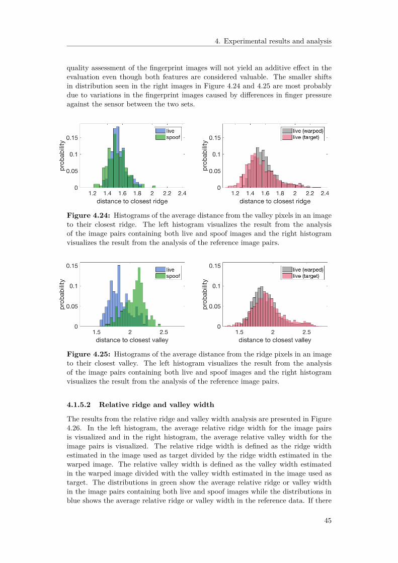
4. Experimental results and analysis

quality assessment of the fingerprint images will not yield an additive effect in theevaluation even though both features are considered valuable. The smaller shiftsin distribution seen in the right images in Figure 4.24 and 4.25 are most probablydue to variations in the fingerprint images caused by differences in finger pressureagainst the sensor between the two sets.

Figure 4.24: Histograms of the average distance from the valley pixels in an imageto their closest ridge. The left histogram visualizes the result from the analysisof the image pairs containing both live and spoof images and the right histogramvisualizes the result from the analysis of the reference image pairs.

Figure 4.25: Histograms of the average distance from the ridge pixels in an imageto their closest valley. The left histogram visualizes the result from the analysisof the image pairs containing both live and spoof images and the right histogramvisualizes the result from the analysis of the reference image pairs.

4.1.5.2 Relative ridge and valley width

The results from the relative ridge and valley width analysis are presented in Figure4.26. In the left histogram, the average relative ridge width for the image pairsis visualized and in the right histogram, the average relative valley width for theimage pairs is visualized. The relative ridge width is defined as the ridge widthestimated in the image used as target divided by the ridge width estimated in thewarped image. The relative valley width is defined as the valley width estimatedin the warped image divided with the valley width estimated in the image used astarget. The distributions in green show the average relative ridge or valley widthin the image pairs containing both live and spoof images while the distributions inblue shows the average relative ridge or valley width in the reference data. If there

45

4. Experimental results and analysis

is a pairwise difference in relative width among the image pairs, the mean of thegreen distributions will be larger than one, while the mean of the reference datadistributions showed in blue should be centered around one.

Figure 4.26: Relative ridge and valley width. The left histogram visualizes therelative ridge width in the image pairs and the right histogram visualizes the relativevalley width in the image pairs. The green distributions shows the average ridgeand valley width ratio in the image pairs containing one live image and one spoofimage. The distributions in blue shows the average ridge and valley width ratio inthe image pairs containing two live images.

As can be seen in Figure 4.26, there are small differences in relative width betweenthe image pairs containing both live and spoof images and the reference image pairs.The difference in relative ridge width is significant at the p = 0.01 level and the dif-ference in relative valley width is significant at the p = 0.025 level. Even though theobtained differences are significant, there are a few limitations of this method whichare believed to have affected the results. First, the resolution of the investigatedfingerprint images is believed to have limited the accuracy of the results obtained inthis analysis. A higher image resolution would have resulted in more precise mea-surements of the ridge and valley widths. Second, noise in the fingerprint patternsuch as spikes, holes and incipient ridges might affect the individual measurementsconsiderably. Third, the irregular ridge and valley interfaces seen in the spoof fin-gerprint images is also believed to limit the accuracy of this analysis. Hence, thereliability of the final statistics might be impaired by these limitations. The relativeridge and valley width was thus not included in the quality assessment model.

Interestingly, it may also be noticed that the mean of the blue distributions origi-nating from the reference image pairs in Figure 4.26 are not centered around one asexpected. This result is however in agreement with the small distribution shifts seenin the right images of Figure 4.24 and 4.25 and is most probably due to variationsin finger pressure against the sensor between the two sets.

4.1.5.3 Frequency spectrum analysis

In Figure 4.27, the average of the radial frequency signals of the source and targetimages in the image pairs are visualized. The plot on the left shows the results fromthe images in the pairs containing one live and one spoof image and the plot on theright shows the results from the reference image pairs. In Figure 4.28, the frequencyspectra magnitudes for an example image pair containing a live and a spoof image

46

4. Experimental results and analysis

are displayed and in Figure 4.29 their radial frequency signals are presented. Theleft image in Figure 4.28 visualizes the frequency spectrum of the spoof image inthe pair and the right image visualizes the frequency spectrum of the live image.

Figure 4.27: Average radial frequency. The left plot visualizes the average radialfrequency of the live and spoof images in the data. The right plot visualizes theaverage radial frequency of the reference data.

Figure 4.28: Frequency spectra magnitude examples. The left image is a typicalexample of the frequency spectrum magnitude of a spoof image and the right imageis a typical example of the frequency spectrum magnitude of a live image. Themagnitude is presented in logarithmic scale in both images.

Figure 4.29: Radial frequency example. The plot visualizes an example of thedifference in radial average frequency often seen between live and spoof images.

As can be seen in Figure 4.27, there is a difference between the average radialfrequency magnitude for the all the live images and the average radial frequencymagnitude for the all the spoof images, compare to the right plot in the same figure

47

4. Experimental results and analysis

in which there is a perfect overlap between the average radial frequency magnitudesignals for the source and target images. The difference between the live and spooffrequency spectra magnitudes becomes even more apparent when studying each pairseparately. The magnitudes of the spoof frequency spectra are in general blurrierthan their live equivalents. In addition to the blurriness, the lobe correspondingto the ridge and valley frequencies are more concentrated in the frequency spectraof the live fingerprint images than in the frequency spectra of the spoof images.These trends can clearly be seen in the example image pair in Figure 4.28. Figure4.29 shows that the difference in the radial frequency obtained from these frequencyspectra magnitudes also is more evident than the average of the radial frequencysignals for all the image pairs. Due to time constraint, this feature was however notincluded in the spoof fingerprint image quality assessment.

4.1.6 Spoof image quality

The predictors used in the hyperplane model and their respective weights are pre-sented in Table 4.1. From the magnitude of the weights presented in this table, it isclear that the intensity profiles are the predictors which have the largest impact inthe hyperplane model. The number of breaks in the valley skeleton and the numberof bifurcations in the ridge skeleton are also given a large impact in the model.

Table 4.1: Hyperplane model predictors and their respective weights. In this tablethe ten features used as predictors in the separating hyperplane model are presentedtogether with their respective weights. The bias term in the model is −0.1086.

hyperplane model predictors β

ridge-valley-ridge intensity profile 1.9123valley-ridge-valley intensity profile -1.5150

number of bifurcations in the ridge skeleton -0.6933number of breaks in the valley skeleton -0.6806

ridge skeleton intensity -0.4656number of spikes in the ridge skeleton -0.3147

distance to closest valley 0.2613number of bifurcations in the valley skeleton 0.1668

number of spikes in the valley skeleton -0.1631ridge skeleton curvature 0.1402

In the 186 image pairs containing both live and spoof images, 162 of the live imagesand 172 of the spoof images are unique. When these unique images are classifiedwith the separating hyperplane model, 66% of the live images and 86% of the spoofimages are classified correctly. Hence, the separating hyperplane model classifies76% of the images in the investigated set correctly. The probability outputs fromthe separating hyperplane model are used as an indication of the spoof image quality.Low quality images are identified by extracting the spoof images with a high spoofprobability while high quality images are identified by extracting the spoof imageswith a low spoof probability. In Figure 4.30 and 4.31, examples of the spoof imageswhich obtained the highest and lowest spoof probability are presented together withtheir live equivalents. The spoof probability of the low quality spoofs displayed in

48

4. Experimental results and analysis

Figure 4.30 are 0.99 while the spoof probability of the high quality spoofs displayedin Figure 4.31 range between 0.06 and 0.16.

Figure 4.30: Examples of low quality spoof images. In the top row of this figurethree of the spoof images with the lowest quality are presented. In the lower rowtheir live equivalents are displayed.

Figure 4.31: Examples of high quality spoof images. In the top row of this figurethree of the spoof images with the highest quality are presented. In the lower rowtheir live equivalents are displayed.

49

4. Experimental results and analysis

The spoof image examples presented in Figure 4.30 and 4.31 clearly demonstratesthe success of the quality assessment. The spoof images in Figure 4.30 are typicalexamples of spoof images which are considered to be easy to differentiate from liveimages, while the images in Figure 4.31 are typical examples of spoofs images inwhich the ridge and valley pattern cannot be differentiated from live ridge andvalley patterns. Hence, the spoof image quality can successfully be estimated fromthe features designed in this thesis. Important to mention is that the low qualityimages presented in Figure 4.30 are not the worst images in the entire data set,since such images did not pass the matching algorithm and thus did not end up inany of the analyzed image pairs. The quality of the spoof images in Figure 4.30is thus low compared to the spoof images in the 186 image pairs, but is still highenough to pass the used matching algorithm. During a manual inspection of thespoof images in Figure 4.31, the circular shapes with high intensity in the left andmiddle spoof image should, however, raise a warning flag. Such circular shapes mayoriginate from dirt on the sensor or from a blister on a live finger, but do oftenoriginate from an air bubble in the spoof material. However, since a realistic ridgeand valley pattern is considered to be the most important feature to assess whenestimating the spoof image quality, the quality of the spoof images in Figure 4.31are still considered as high even though they possess a fairly discriminative feature.

4.2 Learning-based fingerprint liveness classification

In the following sections, the results from the learning-based liveness detection partof the thesis are presented and discussed. Initially, the purpose of the neural networkpart of the thesis was to implement a state-of-the-art liveness detection method forwhich the performance on different data sets could be used as an indication of theirspoof quality. But since the characteristics of fingerprint images are heavily depen-dent on sensor technology, the first network, which was trained on images obtainedwith optical fingerprint sensors, did not manage to generalize to the images obtainedwith the capacitive fingerprint sensing technology used at Fingerprint Cards. Thefirst network could thus not be used to estimate the quality of the spoof imagesprovided by Fingerprint Cards and a second network had to be trained on capaci-tive fingerprint images. Hence, the results obtained from the first network is insteadused as an assurance that the network is successfully implemented.

4.2.1 Network trained on benchmark data

The classification results for each of the test sets used in the Fingerprint LivenessDetection Competition in 2009, 2011 and 2013 are given in Table 4.2. The spooffalse positive rate, the spoof false negative rate and the average classification errorsobtained for the test sets after 30 epochs are given for each of the data sets. Theaverage classification errors previously obtained for the same testing data sets usinga network which had the exact same architecture and which had been trained on thesame data sets are presented within brackets [6] in order to facilitate a comparisonbetween the state-of-the-art results and the results obtained in this thesis.

By studying the average classification errors in Table 4.2, it is clear that the obtainedresults are not quite as impressive as the results presented in [6]. The obtained re-

50

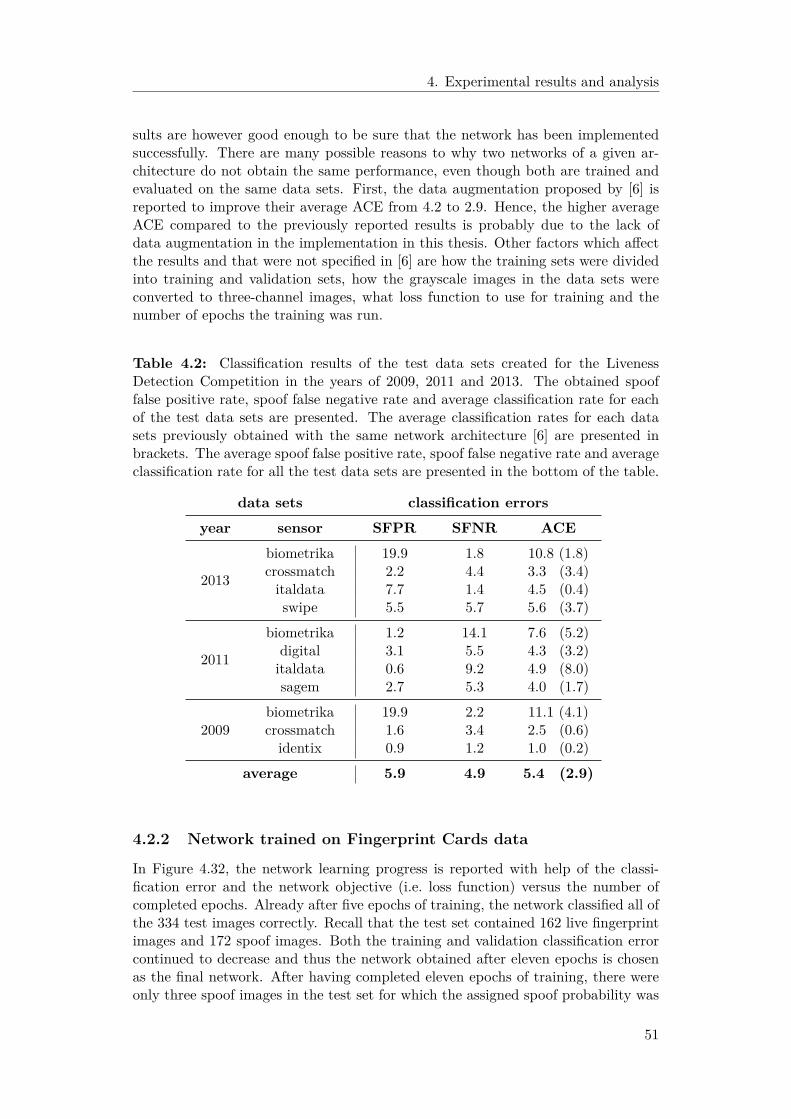
4. Experimental results and analysis

sults are however good enough to be sure that the network has been implementedsuccessfully. There are many possible reasons to why two networks of a given ar-chitecture do not obtain the same performance, even though both are trained andevaluated on the same data sets. First, the data augmentation proposed by [6] isreported to improve their average ACE from 4.2 to 2.9. Hence, the higher averageACE compared to the previously reported results is probably due to the lack ofdata augmentation in the implementation in this thesis. Other factors which affectthe results and that were not specified in [6] are how the training sets were dividedinto training and validation sets, how the grayscale images in the data sets wereconverted to three-channel images, what loss function to use for training and thenumber of epochs the training was run.

Table 4.2: Classification results of the test data sets created for the LivenessDetection Competition in the years of 2009, 2011 and 2013. The obtained spooffalse positive rate, spoof false negative rate and average classification rate for eachof the test data sets are presented. The average classification rates for each datasets previously obtained with the same network architecture [6] are presented inbrackets. The average spoof false positive rate, spoof false negative rate and averageclassification rate for all the test data sets are presented in the bottom of the table.

data sets classification errorsyear sensor SFPR SFNR ACE

2013

biometrika 19.9 1.8 10.8 (1.8)crossmatch 2.2 4.4 3.3 (3.4)italdata 7.7 1.4 4.5 (0.4)swipe 5.5 5.7 5.6 (3.7)

2011

biometrika 1.2 14.1 7.6 (5.2)digital 3.1 5.5 4.3 (3.2)italdata 0.6 9.2 4.9 (8.0)sagem 2.7 5.3 4.0 (1.7)

2009biometrika 19.9 2.2 11.1 (4.1)crossmatch 1.6 3.4 2.5 (0.6)identix 0.9 1.2 1.0 (0.2)

average 5.9 4.9 5.4 (2.9)

4.2.2 Network trained on Fingerprint Cards data

In Figure 4.32, the network learning progress is reported with help of the classi-fication error and the network objective (i.e. loss function) versus the number ofcompleted epochs. Already after five epochs of training, the network classified all ofthe 334 test images correctly. Recall that the test set contained 162 live fingerprintimages and 172 spoof images. Both the training and validation classification errorcontinued to decrease and thus the network obtained after eleven epochs is chosenas the final network. After having completed eleven epochs of training, there wereonly three spoof images in the test set for which the assigned spoof probability was

51

4. Experimental results and analysis

below 0.975. These images are presented in Figure 4.33. The spoof classificationscores of the left, middle and right image are 0.67, 0.87 and 0.97 respectively.

By studying the network learning process in Figure 4.32, it is clear that both theclassification error and the network objective decreases rapidly during the first fewepochs. While the classification accuracy of the test images reaches 100% afterfive epochs, the classification accuracy of the training and validation images is onlymarginally increased from their classification accuracies of 99.95% and 99.50% whichare reached after eleven epochs.

Figure 4.32: Classification error and objective during network training. The leftplot displays the learning progress with help of the classification error both for thetraining and validation set and the right image displays the learning progress withhelp of the network objective for both for the training and validation set.

Figure 4.33: The three best spoofs according to the neural network. These threespoof images yielded the lowest spoof scores. Their spoof scores are however higherthan their liveness scores, hence they are still classified as spoof images.

The fine-tuned network performed far better than expected and classified all theimages in the test set correctly. These results imply that all the images are possibleto classify correctly, regardless of the spoof image quality in the set. However, since

52

4. Experimental results and analysis

the network managed to classify even the most realistic spoof images correctly witha high degree of certainty, this network architecture is not suitable to use in a spoofimage quality assessment. Differentiation between the quality of the images in theset could however possibly be obtained with a more shallow network.

The images presented in Figure 4.33 clearly demonstrates that the spoof imageswhich the network is the least certain of are the ones with ridge and valley patternswhich cannot be differentiated from ridge and valley patterns of live fingerprints.Thus, the network appears to have learned to identify fingerprint images with re-alistic ridge and valley patterns. Moreover, the network has evidently learned todifferentiate obvious spoof images from live fingerprint images.

Important to note is that the left and the middle images in Figure 4.33, which arethe same images that were the most difficult for the network to classify as spoofs,are the images which were assigned the highest quality in the feature design partof the thesis (see Figure 4.31). As previously discussed in Section 4.1.6, the brightcircular shapes in these images probably originate from air bubbles in the spoofs.Since the images in the training set did not contain many spoof images with airbubbles, this is evidently not a feature that the network learned during training.This is, however, a feature which the network probably could learn if the trainingset contained a larger amount of spoof images with this particular feature.

The low quality spoof example images in Figure 4.30, which were assigned the high-est spoof probabilities by the hyperplane model, were also assigned very high spoofprobabilities by the network model. These images were assigned spoof probabili-ties in the range 0.99 − 1.0 by the network. Hence, these three images are easilydifferentiated from live fingerprint images both by the hyperplane model and theconvolutional neural network. The network also assigned a very high spoof proba-bility (0.99) to the rightmost of the high quality spoof images in Figure 4.31. Thefact that the network model assigned almost the same spoof probability to thesefour spoof images substantiates the claim that the structure of the given networkis unsuitable for spoof image quality assessment. The hyperplane model assigneda spoof probability of 0.38 to the rightmost of the images in Figure 4.33. This isconsidered to be a quite high spoof probability for such a realistic spoof image. Apossible explanation for this unexpectedly high spoof probability could be the in-tensity variations along the valleys which may be seen in some areas of the image.

The difference in performance of the two trained networks in this thesis is believedto exist due to the difference in variability within their training and test data sets.The training and test images used in the first network are obtained with eightdifferent sensors and the spoof images in the sets are created with spoofs of eightdifferent materials, while the training and test images used in the second networkare obtained with a single sensor and the spoofs are all made of the same material.

53

4. Experimental results and analysis

54

5Conclusion

The purpose of this thesis was to develop a tool which assesses the quality of spooffingerprint images in a data set and two methods has been evaluated for this pur-pose. The first method was based on manually designed features derived from visualcomparisons of live and spoof images in the data set provided by Fingerprint Cards.Ten of these detected features were found to differ significantly between the live andspoof images and these features were thus used to create a support vector machine-based classifier by identifying the hyperplane model which best separated the liveand spoof fingerprints in the data set. The quality of the spoof images in a data setwas estimated by assessing the number of spoof images that this hyperplane modelmanaged to classify as spoofs. Moreover, the quality of the individual spoof imagesin the set was defined as the liveness probability assigned by the model. Promisingresults were obtained from this quality assessment method. The spoof images thatwere assigned a low quality by the hyperplane model were images which easily couldbe differentiated from their live equivalents in a manual inspection. Conversely, thespoof images that were assigned a high quality were images in which the fingerprintpatterns could not be differentiated from live fingerprint patterns. The presentedresults indicate that the implemented quality assessment was successful for the in-vestigated data set. Further, it shows that the liveness features which were manuallydesigned in this thesis can be used to estimate the spoof image quality.

Features for which there were significant differences between the investigated liveand spoof images originated from the fingerprint skeletons, the fingerprint intensitiesand the ridge and valley patterns of the fingerprint images. The number of breaks inthe valley skeletons and the number of spikes and bifurcations in both the ridge andvalley skeletons were the first five significant liveness features that were constructed.All these features occurred more frequently in spoof fingerprint skeletons than intheir live equivalents. Another significant difference was found when the curvatureof the ridge skeleton was investigated. The curvature of the skeleton is however notbelieved to measure the skeleton jaggedness as intended, but is instead believed tomeasure the larger scale curvature of the skeleton. Although this assessment mightnot function as intended, the curvature of the ridge skeleton is still considered tobe valuable features. The significant features related to the fingerprint intensitieswere the average intensity along the ridge skeletons and the intensity profiles per-pendicular to the ridge and valley patterns in the images. Even though the resultsobtained for the intensity profile features did not agree with the original hypothesis,the differences found was still considered to be a valuable feature. The significantfeature related to the ridge and valley patterns is the average distance to the closestvalley from all the ridge pixels in a fingerprint image. Among these ten features, the

55

5. Conclusion

intensity profiles were given the largest impact in the separating hyperplane modelwhich best separated the two classes. The number of breaks in the valley skeletonsand the number of bifurcations in the ridge skeletons were also given a relativelylarge impact in the separating hyperplane model.

The second method evaluated for spoof image quality assessment purposes was basedon a convolutional neural network from which state-of-the-art liveness classificationresults recently has been reported on benchmark data sets. The initial idea wasto estimate the spoof image quality of a data set based on the classification resultsobtained when the set was classified with the state-of-the-art liveness classificationnetwork. This network was however trained on images obtained from optical fin-gerprint sensors and did not manage to generalize to fingerprint images obtainedfrom capacitive sensors due to their different characteristics. By training the samenetwork architecture on fingerprint images obtained from capacitive sensors insteadof images obtained from optical sensors, a capacitive version of the state-of-the-artliveness detection network was created. The performance of this liveness detectionnetwork was far better than expected, the network classified all the live and spoofimages in the investigated set correctly and only three of the spoof images wereassigned a spoof probability lower than 0.975. These are fantastic liveness detec-tion results. However, the fact that the network managed to classify even the mostrealistic spoof images correctly with a high degree of certainty makes this networkarchitecture unsuitable for spoof quality assessment. Differentiation between theimages in the set could however possibly be obtained with a more shallow network.

Since the implemented liveness detection network demonstrated such extraordinaryperformance, it is suggested that future studies investigate the network in moredetail. There are methods to investigate the features learned by the network [33, 34]and by identifying such features a better understanding of the liveness detectionperformed by the network might be obtained. Also, by investigating the networkin more detail it could probably be reduced in size which could make it suitable forusage in on-line applications such as mobile phones.

56

Bibliography

[1] A. K. Jain et al., Introduction to Biometrics, pp. 1–10, 44–47, 51–81. Springer, 2014.

[2] D. Maltoni et al., Handbook of Fingerprint Recognition, ch. 1, 2, 3, 4, 5, 8, 9. Springer, 2009.

[3] S. Marcel et al., eds., Handbook of Biometric Anti-Spoofing - Trusted Biometrics under SpoofingAttacks, pp. 1–10, 35–43. Advances in Computer Vision and Pattern Recognition, Springer,2014.

[4] Fingerprint Cards AB. https://www.fingerprints.com [2016-10-17].

[5] L. Ghiani et al., “Review of the Fingerprint Liveness Detection (LivDet) competition series:2009 to 2015,” Image and Vision Computing, 2016.

[6] R. F. Nogueira et al., “Fingerprint liveness detection using convolutional neural networks,”IEEE Transactions on Information Forensics and Security, vol. 11, no. 6, pp. 1206–1213,2016.

[7] D. Gragnaniello et al., “Local contrast phase descriptor for fingerprint liveness detection,”Pattern Recognition, vol. 48, no. 4, pp. 1050–1058, 2015.

[8] D. Gragnaniello et al., “An investigation of local descriptors for biometric spoofing detection,”IEEE Transactions on Information Forensics and Security, vol. 10, no. 4, pp. 849–863, 2015.

[9] L. Ghiani et al., “Fingerprint liveness detection using binarized statistical image features,” inIEEE International Conference on Biometrics: Theory, Applications and Systems, 2013.

[10] J. Galbally et al., “A high performance fingerprint liveness detection method based on qualityrelated features,” Future Generation Computer Systems, vol. 28, no. 1, pp. 311–321, 2012.

[11] E. Lim et al., “Fingerprint quality and validity analysis,” in IEEE International Conferenceon Image Processing, vol. 1, pp. 469–472, 2002.

[12] Y. Chen et al., “Fingerprint quality indices for predicting authentication performance,” in In-ternational Conference on Audio- and Video-Based Biometric Person Authentication, pp. 160–170, Springer, 2005.

[13] P. Coli et al., “Fingerprint silicon replicas: static and dynamic features for vitality detectionusing an optical capture device,” International Journal of Image and Graphics, vol. 8, no. 4,pp. 495–512, 2008.

[14] T. P. Chen et al., “Fingerprint image quality analysis,” in IEEE International Conference onImage Processing, vol. 2, pp. 1253–1256, 2004.

[15] L. Hong et al., “Fingerprint image enhancement: algorithm and performance evaluation,”IEEE Transactions on Pattern Analysis and Machine Intelligence, vol. 20, no. 8, pp. 777–789,1998.

[16] M. Kücken and A. C. Newell, “Fingerprint formation,” Journal of Theoretical Biology, vol. 235,no. 1, pp. 71–83, 2005.

57

Bibliography

[17] R. Cappelli and D. Maltoni, “On the spatial distribution of fingerprint singularities,” IEEETransactions on Pattern Analysis and Machine Intelligence, vol. 31, no. 4, pp. 742–748, 2008.

[18] A. M. Bazen and S. H. Gerez, “Segmentation of fingerprint images,” in ProRISC Workshopon Circuits Systems and Signal Processing, pp. 276–280, 2001.

[19] A. M. Bazen and S. H. Gerez, “Directional field computation for fingerprints based on theprincipal component analysis of local gradients,” in ProRISC Workshop on Circuits Systemsand Signal Processing, pp. 215–222, 2000.

[20] R. C. Gonzalez and R. E. Woods, Digital image processing, pp. 649–675, 764–765, 834–837.Pearson Prentice Hall, 2010.

[21] P. Soille, Morphological image analysis: principles and applications, pp. 1–10. Springer, 2013.

[22] I. Goodfellow et al., Deep Learning, pp. 1–26, 330–372. Adaptive Computation and MachineLearning series, The MIT Press, 2016.

[23] M. A. Nielsen, Neural Networks and Deep Learning, ch. 1, 2, 6. Adaptive Computation andMachine Learning series, Determination Press, 2016.

[24] Y. LeCun et al., “Convolutional networks and applications in vision,” in International Sym-posium on Circuits and Systems, pp. 253–256, 2010.

[25] A. Vedaldi and K. Lenc, “MatConvNet – Convolutional Neural Networks for MATLAB,” inACM International Conference on Multimedia, 2015.

[26] R. A. Adams and C. Essex, Calculus: a complete course, pp. 867–873. Pearson Canada, 8 ed.,2013.

[27] M. Sonka et al., Image Processing, Analysis, and Machine Vision, pp. 337–339. CengageLearning, 2014.

[28] V. Mura et al., “LivDet 2015 – Fingerprint Liveness Detection Competition 2015,” in IEEEInternational Conference on Biometrics Theory, Applications and Systems, 2015.

[29] G. L. Marcialis et al., “First International Fingerprint Liveness Detection Competition –LivDet 2009,” in International Conference on Image Analysis and Processing, pp. 12–23, 2009.

[30] D. Yambay et al., “LivDet 2011 – Fingerprint Liveness Detection Competition 2011,” in In-ternational Conference on Biometrics (ICB), pp. 208–215, 2012.

[31] L. Ghiani et al., “LivDet 2013 – Fingerprint Liveness Detection Competition 2013,” in Inter-national Conference on Biometrics (ICB), pp. 1–6, 2013.

[32] K. Simonyan and A. Zisserman, “Very deep convolutional networks for large-scale image recog-nition,” in International Conference on Learning Representations, 2015.

[33] M. D. Zeiler and R. Fergus, “Visualizing and understanding convolutional networks,” in Eu-ropean Conference on Computer Vision, pp. 818–833, 2014.

[34] R. Girshick et al., “Rich feature hierarchies for accurate object detection and semantic seg-mentation,” in IEEE Conference on Computer Vision and Pattern Recognition, pp. 580–587,2014.

58