feasibility of deception in code attribution
TRANSCRIPT

Feasibility of Deception in Code Attribution
by
Alina Matyukhina
Master of Mathematics, DonNU, 2017Bachelor of Mathematics with Honors, DonNU, 2015
A DISSERTATION SUBMITTED IN PARTIAL FULFILLMENT OFTHE REQUIREMENTS FOR THE DEGREE OF
Doctor of Philosophy
In the Graduate Academic Unit of Faculty of Computer Science
Supervisor(s): Natalia Stakhanova, Ph.D., Computer ScienceExamining Board: Rongxing Lu, Ph.D., Computer Science,
Suprio Ray, Ph.D., Computer Science,Martin Wielemaker, Ph.D., Business Administration
External Examiner: Mohammad Zulkernine, Ph.D., School of Computing,Queen’s University
This dissertation is accepted
Dean of Graduate Studies
THE UNIVERSITY OF NEW BRUNSWICK
August, 2019
c©Alina Matyukhina, 2019

Abstract
Code authorship attribution is the process used to identify the probable author
of given code, based on unique characteristics that reflect an author’s program-
ming style. Inspired by social studies in the attribution of literary works, in the
past two decades researchers have examined the effectiveness of code attribution in
the computer software domain, including computer security. Authorship attribution
techniques have found a broad application in code plagiarism detection, biometric re-
search, forensics, and malware analysis. Studies show that analysis of software might
effectively unveil the digital identity of a programmer, reflected through variables and
structures, programming language, employed development tools, their settings and,
more importantly, how and what these tools are being used to do.
Authorship attribution has been a prosperous area of research when an assumption
can be made that the author of an unknown program has been honest in their writing
style and does not try to modify it. In this thesis, we investigate the feasibility of
deception of source code attribution techniques.
We begin by exploring how data characteristics and feature selection influence both
the accuracy and performance of attribution methods. Within this context, it is
necessary to understand whether the results obtained by previous studies depend on
the data source, quality, and context or the type of features used. It gives us the
opportunity to dive deeper into the process of code authorship attribution to be able
to understand its potential weaknesses.
ii

To evaluate current code attribution systems, we present an adversarial model de-
fined by the adversary’s goals, knowledge, and capabilities; for each group, we cate-
gorize them by the possible variations. Modeling the role of attackers figures promi-
nently in enhancing the cybersecurity defense. We believe that having a solid under-
standing of the possible attacks can help in the research and deployment of reliable
code authorship attribution systems.
We present an author imitation attack that deceives current authorship attribution
systems by imitating a coding style of a targeted developer. We investigate the
attack’s feasibility on open-source software repositories.
To subvert an author imitation attack and to help in protecting the developer’s pri-
vacy, we introduce an author obfuscation method and novel coding style transforma-
tions. The idea of author obfuscation is to allow authors to preserve the readability of
their source code while removing identifying stylistic features that can be leveraged
for code attribution. Code obfuscation, common in software development, typically
aims to disguise the appearance of the code making it difficult to understand and
reverse engineer. In contrast, the proposed author obfuscation hides the original
author’s style by leaving the source code visible, readable and understandable.
In summary, this thesis presents original research work that not only advances the
knowledge in code authorship attribution field but also contributes to the overall
safety of our digital world by providing author obfuscation methods to protect the
privacy of the developers.
iii

Dedication
To
My Mother
My greatest teacher, who teaches me compassion, love, and fearlessness
My Father
My mentor, example, and guide; who always encourages me and cheers for me
My Sister
My best friend, my soulmate; who knows my thoughts without a word
My Love
My greatest gift, who has a quiet strength that makes my heart sing
iv

Acknowledgements
I would like to thank my parents, my sister, my boyfriend and his family for sup-
porting me during my PhD and every moment in my life.
I would like to thank my supervisor, Canada Research Chair in Security and Privacy,
Dr. Natalia Stakhanova for providing her guidance and suggestions.
I am also grateful to Dr. Mila Dalla Preda for her help.
I am very thankful to my examining committee members for their precious time,
patience, and support.
I also thank all my colleagues from the Canadian Institute for Cybersecurity for their
coordination and cooperation.
I would like to thank all the academic and administrative staff of the University of
New Brunswick for their kindness and help.
v

Table of Contents
Abstract ii
Dedication iv
Acknowledgments v
Table of Contents viii
List of Tables ix
List of Figures xi
1 Introduction 1
1.1 Problem Statement and Motivation . . . . . . . . . . . . . . . . . . . 2
1.2 Contributions . . . . . . . . . . . . . . . . . . . . . . . . . . . . . . . 4
1.3 Thesis Organization . . . . . . . . . . . . . . . . . . . . . . . . . . . . 5
2 Literature Review 7
2.1 Code authorship attribution . . . . . . . . . . . . . . . . . . . . . . . 7
2.1.1 Reviewed studies . . . . . . . . . . . . . . . . . . . . . . . . . 9
2.1.2 Datasets . . . . . . . . . . . . . . . . . . . . . . . . . . . . . . 16
2.1.3 Features . . . . . . . . . . . . . . . . . . . . . . . . . . . . . . 20
2.2 Summary . . . . . . . . . . . . . . . . . . . . . . . . . . . . . . . . . 23
3 Adversarial code attribution 25
vi

3.1 Author imitation attack . . . . . . . . . . . . . . . . . . . . . . . . . 26
3.2 Author obfuscation . . . . . . . . . . . . . . . . . . . . . . . . . . . . 29
3.3 Coding style transformations . . . . . . . . . . . . . . . . . . . . . . . 30
3.3.1 Layout transformations . . . . . . . . . . . . . . . . . . . . . . 30
3.3.2 Lexical transformations . . . . . . . . . . . . . . . . . . . . . . 35
3.3.3 Syntactic transformations . . . . . . . . . . . . . . . . . . . . 36
3.3.4 Control-flow transformations . . . . . . . . . . . . . . . . . . . 37
3.3.5 Data-flow transformations . . . . . . . . . . . . . . . . . . . . 41
3.4 Summary . . . . . . . . . . . . . . . . . . . . . . . . . . . . . . . . . 44
4 Assessing effects of dataset characteristics on attribution perfor-
mance 45
4.1 Replication study . . . . . . . . . . . . . . . . . . . . . . . . . . . . . 47
4.1.1 Experimental setup . . . . . . . . . . . . . . . . . . . . . . . . 49
4.1.2 Evaluation . . . . . . . . . . . . . . . . . . . . . . . . . . . . . 53
4.1.3 Dataset analysis . . . . . . . . . . . . . . . . . . . . . . . . . . 53
4.1.4 Correlation analysis of features from previous studies . . . . . 59
4.2 Impact of dataset characteristics on the performance . . . . . . . . . 61
4.2.1 How long should code samples be? . . . . . . . . . . . . . . . 62
4.2.2 How many samples per author are needed? . . . . . . . . . . . 64
4.2.3 How many authors are needed? . . . . . . . . . . . . . . . . . 67
4.2.4 What features are the best? . . . . . . . . . . . . . . . . . . . 70
4.3 Summary . . . . . . . . . . . . . . . . . . . . . . . . . . . . . . . . . 78
5 Evaluation 81
5.1 Evaluation of authorship attribution methods . . . . . . . . . . . . . 81
5.2 Adversarial model for code attribution . . . . . . . . . . . . . . . . . 85
5.3 Author imitation evaluation . . . . . . . . . . . . . . . . . . . . . . . 87
vii

5.4 Evaluation of coding style transformations based on the metrics . . . 90
5.4.1 Complexity . . . . . . . . . . . . . . . . . . . . . . . . . . . . 91
5.4.2 Readability . . . . . . . . . . . . . . . . . . . . . . . . . . . . 96
5.4.3 Resilience . . . . . . . . . . . . . . . . . . . . . . . . . . . . . 98
5.4.4 Cost . . . . . . . . . . . . . . . . . . . . . . . . . . . . . . . . 99
5.4.5 Detection . . . . . . . . . . . . . . . . . . . . . . . . . . . . . 100
5.4.6 Results . . . . . . . . . . . . . . . . . . . . . . . . . . . . . . . 100
5.5 Author obfuscation techniques evaluation . . . . . . . . . . . . . . . . 110
5.6 Threats to validity . . . . . . . . . . . . . . . . . . . . . . . . . . . . 118
5.7 Summary . . . . . . . . . . . . . . . . . . . . . . . . . . . . . . . . . 122
6 Conclusion and Future work 123
Bibliography 138
A Our improved features 139
A.1 List of our improved features for datasets with 1 to 50 LOC . . . . . 139
A.2 List of our improved features for datasets with 51 to 100 LOC . . . . 140
A.3 List of our improved features for datasets with 101 to 200 LOC . . . 143
A.4 List of our improved features for datasets with 201 to 300 LOC . . . 147
A.5 List of our improved features for datasets with 301 to 400 LOC . . . 149
A.6 List of our improved features for datasets with 401 plus LOC . . . . 151
Vita
viii

List of Tables
2.1 Previous studies in source code authorship attribution. . . . . . . . . 10
4.1 The results of replication study . . . . . . . . . . . . . . . . . . . . . 54
4.2 Accuracy of attribution after removing common code . . . . . . . . . 57
4.3 Correlation coefficient analysis for Caliskan features . . . . . . . . . . 60
4.4 Accuracy with uncorrelated features (401 plus 75 authors dataset) . . 61
4.5 The datasets grouped by LOC . . . . . . . . . . . . . . . . . . . . . . 63
5.1 The details of our datasets and feature sets employed by previous
studies. . . . . . . . . . . . . . . . . . . . . . . . . . . . . . . . . . . . 83
5.2 Percentage of successfully imitated authors . . . . . . . . . . . . . . . 90
5.3 Applied transformations and their evaluation . . . . . . . . . . . . . . 109
5.4 Effect of information gain feature selection using Caliskan et al. [44]
approach . . . . . . . . . . . . . . . . . . . . . . . . . . . . . . . . . . 113
5.5 Results of author obfuscation methods on all datasets . . . . . . . . . 117
ix

List of Figures
2.1 Timeline of attribution studies and the corresponding sources of the
experimental datasets. . . . . . . . . . . . . . . . . . . . . . . . . . . 18
2.2 Dependence between number of authors and accuracy in the existing
studies. The insert gives statistics for 3 outliers. . . . . . . . . . . . . 19
2.3 Feature selection levels in code authorship attribution . . . . . . . . 21
3.1 An overview of author imitation attack . . . . . . . . . . . . . . . . 27
3.2 Curly brackets styles . . . . . . . . . . . . . . . . . . . . . . . . . . . 32
3.3 Control-flow flattening transformations (with ”switch” and normal
dispatch) . . . . . . . . . . . . . . . . . . . . . . . . . . . . . . . . . 38
3.4 Opaque predicate transformations . . . . . . . . . . . . . . . . . . . 40
4.1 Presence of common code in datasets. . . . . . . . . . . . . . . . . . 56
4.2 The changes in accuracy with respect to the amount of common code 59
4.3 Example of source code and its AST . . . . . . . . . . . . . . . . . . 61
4.4 Accuracy vs LOC . . . . . . . . . . . . . . . . . . . . . . . . . . . . . 63
4.5 The impact of varying number of samples per author . . . . . . . . . 66
4.6 The impact of varying number of authors on accuracy . . . . . . . . 66
4.7 Attribution accuracy with varying number of samples and number of
authors on the example of Ding feature set . . . . . . . . . . . . . . . 70
4.8 Attribution accuracy of Caliskan features, TF unigram, and AST bi-
grams on different LOC datasets . . . . . . . . . . . . . . . . . . . . . 71
x

4.9 Attribution accuracy with byte and token n-gram features on 1 to 50
LOC dataset after information gain feature selection . . . . . . . . . 73
4.10 Number of n-gram features before and after information gain feature
selection on 1 to 50 LOC dataset . . . . . . . . . . . . . . . . . . . . 74
4.11 Performance of byte and token n-gram features on datasets with dif-
ferent code size after information gain feature selection . . . . . . . . 75
4.12 Performance of byte n-gram features on a datasets with different num-
ber of authors . . . . . . . . . . . . . . . . . . . . . . . . . . . . . . . 76
4.13 Performance of token n-gram features with different number of authors 77
4.14 Attribution accuracy with the improved feature set on 75 authors
dataset with 10 samples per author . . . . . . . . . . . . . . . . . . . 77
5.1 Confusion matrices for all three scenarios . . . . . . . . . . . . . . . . 89
5.2 Percentage of correctly classified authors after using the following
formatting: Beatify, Code Convention and PrettyPrinter on original
source code . . . . . . . . . . . . . . . . . . . . . . . . . . . . . . . . 110
5.3 Percentage of correctly classified authors after brackets transformation
for GoogleCodeJam Java dataset . . . . . . . . . . . . . . . . . . . . 111
xi

Chapter 1
Introduction
Digital forensics becomes very important when issues about authors of documents
arise, such as their identity and characteristics (age, gender, native language, or
psychometric traits) and ability to associate them with unknown documents.
The study of authorship attribution (also known as stylometry) comes from the
literary domain where it is typically applied to identify an author of a disputed
text based on the author’s unique linguistic style (e.g., use of verbs, vocabulary,
sentence length). The central premise of stylometric techniques lies in the assumption
that authors unconsciously tend to use the same linguistic patterns. These patterns
comprise a number of distinctive features that allow us to characterize an author’s
style and uniquely identify their works.
Drawing an analogy between an author and a software developer, code authorship
attribution aims to decide who wrote a computer program, given its source or binary
code. Applications of code authorship attribution are wide and include any scenario
where code ownership needs to be determined, for example:
• software forensics: where the analyst wants to determine the author of a suspi-
cious program given a set of potential adversaries;
• plagiarism detection: where the analyst wants to identify illicit code reuse;
1

• programmer de-anonymization: where the analyst is interested in finding in-
formation on an anonymous programmer.
Traditionally, authorship attribution studies relied on a large set of samples to gen-
erate accurate representation of an authors style. A recent study by Dauber et
al. [54] showed that this is no longer necessary and even small, and incomplete code
fragments can be used to identify the developers of samples with up to 99% accuracy.
Authorship attribution has been a prosperous area of research when an assumption
can be made that the author of an unknown program has been honest in their
writing style and did not try to modify it. In this dissertation, we investigate the
feasibility of deception in source code attribution techniques. We explore state-of-
the-art authorship attribution and its potential to be circumvented. Our research
aims to examine the resiliency of existing attribution methods to obfuscation and
their susceptibility to circumvention attacks.
1.1 Problem Statement and Motivation
The area of deception in source code authorship attribution has not been significantly
explored. Although current authorship attribution techniques are highly accurate
in detecting authors in “laboratory conditions” [8], such as a single-authored code
submitted to the GoogleCodeJam competition, the ability to use these techniques in
open-source software repositories, with a code written ’in the wild’, is still scarcely
investigated.
The first challenge is to determine if current authorship attribution techniques rec-
ognize authors correctly after they imitate another’s identity. For example, one can
easily see that by imitating someone’s coding style it is possible to implicate any
software developer in wrongdoing. One potential scenario of such an attack may be
realized when a malware developer is trying to cover their tracks by imitating some-
2
one else’s coding style. All it would take is selecting a victim and accessing their
software samples available on an open-source repository, e.g., Github. Then, lifting
the coding style features from the victim’s code samples to mimic their style. Would
it be enough to confuse attribution techniques and create an erroneous assumption
that the malware is written by an unsuspecting contributor of GitHub? If yes, the
attack can be applied in any open-source platform and therefore is a serious threat
to an open-source user’s privacy.
The second challenge is whether or not the authors can protect their identity (i.e.,
coding style) in open-source projects. Open-source software is open to anyone by
design, whether it is a community of developers, hackers, or malicious users. Authors
of open-source software typically hide their identity through nicknames and avatars.
However, they have no protection against authorship attribution techniques that can
create code author profiles just by analysing software characteristics.
To summarize the first and second challenges, both offensive and defensive scenarios
are possible, such as an author imitation attack (imitating another author) and
author obfuscation (protecting the coding style of the original author). An imitation
is successful if an attacker has circumvented a code attribution system into expecting
that the source code came from a victim, who did not create this code. A successful
obfuscation means that an author can modify the code to hide their true authorship.
The lack of research into the field of source code authorship attribution is also a
challenge. Advances in authorship attribution are raising interest in whether or not
it can be used in open-source projects. While there are many legitimate reasons for
an author to wish to remain anonymous, there are also many reasons for wanting to
unmask an unknown author of the software, notably malware creators who try to
hide their identity or to mimic a legitimate user’s coding style.
We pose the main research question that underlines the proposed research:
Are current code authorship attribution techniques resilient to deception?
3

To answer this question, firstly, we developed systematization of features and datasets
used in source code authorship attribution. This systematization offered a compre-
hensive overview of the existing research in this field and provided us an under-
standing of the attribution specifics. Secondly, we analysed the unique features used
in source code attribution in general and systemized them into categories. The
extracted features could lay a foundation for a more effective and accurate author-
ship attribution system. Thirdly, we analysed how dataset characteristics influence
attribution accuracy. Finally, we developed an author imitation attack to deceive
current authorship attribution techniques. We investigated the attack’s feasibility in
open-source software projects. As this attack could affect the privacy of open-source
developers, we proposed practical solutions to hide the author’s style.
1.2 Contributions
We envision the following research contributions:
RC1: An attack against authorship attribution. We developed an author
imitation attack that deceives current authorship attribution systems and mimic the
coding style of a targeted developer.
RC2: A new author obfuscation technique for proprietary and open-
source software. We designed a set of coding style transformations. Unlike ex-
isting code transformations, which work towards concealing the specific details in
the program (data structures and algorithms, the logic of the program, keys and
passwords) [33], the coding style transformations obscure only the writing style of
developers. We envisioned two potential application domains of our author obfus-
cation technique: for use in proprietary software (a source that does not need to
remain readable) and open-source software (readability is a crucial factor for such
software).
4

RC3: Automated measures for evaluation of author obfuscation methods
We proposed to assess our obfuscation transformations using the following metrics:
• complexity: How complex has the program become after the author obfuscation
compared to the original?
• readability: How easy is it for a human to read and understand the obfuscated
code?
• resilience: How difficult is it to construct an automatic tool that can undo the
author obfuscation and return the code to the original author’s coding style?
• cost: How much the execution time and space of the program changed after author
obfuscation?
• detection: Are the authorship attribution techniques currently known today still
able to detect the author of the obfuscated code?
RC4: An optimal set of data characteristics for authorship attribution
task We explored the suitable data characteristics, such as the number of authors,
samples per author, and length of samples necessary for the code attribution task.
RC5: A comprehensive open-source dataset for authorship attribution.
We designed an approach to construct authorship attribution datasets from open-
source repositories.
1.3 Thesis Organization
The rest of the thesis is organized as follows:
• Chapter 2: Background and Literature Review discusses the background of
code authorship attribution by used datasets and features. A comparison is
also made between prominent attribution studies.
5

• Chapter 3: Adversarial code attribution describes our proposed author im-
itation attack and author obfuscation techniques and presents coding style
transformations.
• Chapter 4: Assessing effects of dataset characteristics begins with the anal-
ysis of the data employed by the existing studies in the area of source code
attribution and replicating their experiments. It proceeds with exploring the
effect of common code, source code size, samples size, and author set size on
attribution accuracy. Finally, it describes a large-scale authorship attribution
dataset, which we offer to the research community.
• Chapter 5: Evaluation explores the accuracy of attribution using currently ex-
isting authorship attribution techniques in the presence of deception. Then the
feasibility of an author imitation attack is investigated on open-source software
repositories. It describes the results of coding style transformations and au-
thor obfuscation methods based on complexity, readability, resilience, cost, and
detection.
• Chapter 6: Conclusion and Future work concludes the thesis with the find-
ing’s summary, challenges, and limitations of conducting the research, and
some remarks on future work.
6

Chapter 2
Literature Review
In this chapter, we cover a fundamental introduction to the code authorship attribu-
tion process. We also offer a literature review related to this research. Section 2.1.1
covers summarization of each study in code authorship attribution and discusses the
strengths and weaknesses of their methods. In Section 2.1.2 and Section 2.1.3, we
are analysing the existing attribution techniques by using datasets and features to
emphasize the current challenges in the field.
2.1 Code authorship attribution
Authorship attribution, also known as stylometry, is a well-known research subject
in the literary domain. Dating back to the 19th century and the first authorship
analysis of Shakespeare poems, authorship attribution techniques leveraged research
developments in machine learning and natural language processing fields, quickly
crossing into attribution of electronic texts (e.g., email messages, blog posts, web
pages), software, source, and binary code samples.
Code authorship attribution refers to the process of identifying the probable au-
thor of a given source/binary code based on its unique characteristics that reflect
the author’s programming style. Inspired by social studies in the attribution of
7

literary works, in the past two decades researchers examined the effectiveness of
code attribution in the computer software domain, including computer security. Au-
thorship attribution techniques have found a wide application in code plagiarism
detection [113, 84, 57], biometric research [74], forensics [127, 96], and malware anal-
ysis [27, 46].
The uniqueness of code attribution lies in the characteristics of a fingerprint and its
ability to quantify the author’s programming style. One of the main difficulties in
the field is in compiling a fingerprint that provides an efficient and accurate char-
acterization of an author’s style. In the traditional setting, authorship attribution
relies heavily on information that allows more in-depth linguistic analysis of an au-
thor’s works (e.g., the richness of vocabulary, tense of verbs, semantic analysis of
sentences). In the software field, the researchers often emphasize the surface charac-
teristics: use of variables and structures, programming language, development tools,
and their settings and, more importantly, on how and why these tools are being used.
Since the binary code retains only a few of the surface characteristics, more research
so far has been done in source code authorship attribution.
Traditionally, the process of the source code authorship attribution follows three
steps:
• Dataset collection In this step, reliable datasets of the source code of programs
are obtained from various sources.
• Features extraction and representation In this step, features are extracted
from the programs in the dataset, then those features are represented in an
appropriate form.
• Authorship attribution In this step, a program is assigned to an author.
8

2.1.1 Reviewed studies
In this section, we summarize the primary studies in source code authorship attri-
bution and discuss the strengths and weaknesses of their methods. Table 2.1 gives
a summary of previous studies based on the choice of the authorship features, the
size of the dataset, the data source, the choice of programming language, and the
classification method used.
The first in-depth study of source code authorship attribution was performed by
Krsul et al. [92]. The researchers leveraged C programs collected from students,
faculty, and staff to study the impact of programming structure (e.g., lines of code
per function and number of void functions), programming style (e.g., variable and
function name length), and programming layout (e.g., indentation and whitespace)
on attribution. This study experimented with over 20 different classification meth-
ods on a small set of 88 programs from 29 programmers (on average 3 samples per
author). The obtained accuracy varied drastically between 70% and 100% depending
on the algorithm and normalization technique. For this analysis (with the exception
of discriminant analysis) authors used 4-fold cross validation that is likely to intro-
duce bias in this result only due to lack of a sufficient number of samples per author.
For this reason in Table 2.1 we only list the classification accuracy of discriminant
analysis (73%).
MacDonell et al. [96] utilized three machine learning techniques for authorship
attribution: neural networks, multiple discriminant analysis, and case-based reason-
ing. The authors concluded that the case-based reasoning (CBR) approach yielded
the best results. The dataset included programs from textbooks and experienced
programmers. Although this dataset only consisted of programs of 7 authors, the
number of samples and size of sampled varied drastically between authors, e.g., some
authors only had 5 samples, while others had over 100 programs. Such difference
among authors raised questions about the accuracy of the obtained results [39].
9

Table 2.1: Previous studies in source code authorship attribution.
Related Work Year NumberAu-thors
RangeSamples/Author
TotalFiles
RangeLOC
AverageLOC
NumberFea-tures
Type Fea-tures
Lang Dataset Method Result
Krsul et al. [92] 1997 29 - 88 - - 49 lay,lex C academic LDA 73%
MacDonell et al.[96] 1999 7 5-114 351 16-1480* 182* 26 lay,lex C++ mixed CBR 88%Pellin et al. [109] 2000 2 1360-7900 - - - - synt Java multiple OSSs SVM 73%Ding et al.[55] 2004 46 4-10 259 200-2000 - 56 lay,lex Java mixed CDA 67.2%
Frantzeskou et al. [73] 2006 30 4-29* 333* 20-980* 172* 1500 lex Java FreshMeat(OSS) SCAP 96.9%
Frantzeskou et al. [73] 2006 8 6-8 60* 36-258 129 2000 lex Java academic SCAP 88.5%Frantzeskou et al. [73] 2006 8 4-30 107 23-760 145 1500 lex Java FreshMeat(OSS) SCAP 100%Kothari et al. [91] 2007 8 - 220 - - 50 lex - academic NaiveBayes 69%Kothari et al. [91] 2007 12 - 2110 - - 50 lex - multiple OSSs NaiveBayes 61%
Lange et al. [94] 2007 20 3 60 336-80131* 11166 18 lay,lex Java SourceForge(OSS) NNS 55.0%
Elenbogen et al. [60] 2008 12 6-7 83 50-400* 100* 6 lay,lex C++* academic C4.5 DT 74.70%Burrows et al. [41] 2009 10 14-26 1597 1-10789 830 325 lex C academic ranking 76.78%Shevertalov et al. [124] 2009 20 5-300 - - 11166 163 lay,lex Java SourceForge(OSS) genetic 54.3%Bandara et al. [30] 2013 10 28-128 780 28-15052 44620 9 lay,lex Java SourceForge(OSS) regression 93.64%Bandara et al. [30] 2013 9 35-118 520 20-1135 6268 9 lay,lex Java academic regression 89.62%Tennyson et al. [133] 2014 15 4-29 7231 1-3265 50 - lex C++ mixed Ensemble 98.2%Caliskan et al. [44] 2015 250 9 2250 68-83 70 120000 lay,lex,synt C++ GoogleCodeJam RF 98.04%Caliskan et al. [44] 2015 1600 9 14400 68-83 70 - lay,lex,synt C++ GoogleCodeJam RF 92.83%Wisse et al. [142] 2015 34 - - - - 1689 lay,lex,synt JS GitHub(OSS) SVM 85%Yang et al. [144] 2017 40 11-712 3022 16-11418 98.63 19 lay,lex,synt Java GitHub(OSS) PSOBP 91.1%Alsulami et al. [28] 2017 10 20 200 - - 53 synt C++ GitHub(OSS) BiLSTM 85%Alsulami et al. [28] 2017 70 10 700 - - 130 synt Python GoogleCodeJam BiLSTM 88.86%Gull et al. [78] 2017 9 - 153 100-12000 - 24 lay, lex Java PlanetSourceCode(OSS) NaiveBayes 75%Zhang et al. [147] 2017 53 - 502 - - 6043 lay,lex Java PlanetSourceCode(OSS) SMO 83.47%Dauber et al. [54] 2017 106 150 15900 1-554 4.9 451368 lay,lex, synt C++ GitHub(OSS) RF 70%
McKnight et al. [103] 2018 525 2-11 1261 27-3791* 336* 265 lay,lex, synt C++ GitHub(OSS) RF 66.76%
Simko et al. [125] 2018 50 7-61* 805 10-297* 74* - lay,lex, synt C GoogleCodeJam RF 84.5%*
- No data* Data obtained from personal communication
10

Most of the authorship attribution techniques extract features from the source code
such as variable names and keyword frequencies. Instead of using layout and lexical
features, Pellin et al. [109] used only syntactic features derived from the abstract
syntax trees. The approach was unique as instead of creating frequency-based feature
vectors (common in attribution), the authors feed the abstract syntax tree directly
to the tree-based kernel machine classifier. Unfortunately, the analysis with only 2
authors does not provide sufficient ground for comparison with other methods.
Ding et al. [55] study was based primarily on 49 originally proposed by Krsul et
al. [92], yet additional features described by MacDonell et al. [96] and Gray et al. [75]
were also considered. The authors adapted their C/C++ features for Java language
and used statistical analysis to measure their contribution. Out of the 56 extracted
metrics, 48 metrics were selected for authorship identification. Although the final list
of features was never identified, the researchers indicated the superiority of layout
metrics.
Instead of using software metrics, Frantzeskou et al. [73] considered byte-level
n-grams. In their work, the researchers introduced SCAP (Source Code Author
Profiles) approach, representing a source code author’s style through byte-level n-
gram profiles. Since an author profile is comprised of a list of the L most frequent
n-grams, several follow-up studies were performed to determine the best values of
L and n [68, 72, 73, 71, 69, 70, 67]. The best results were achieved for values of L
equal to 1500 or 2000 and n-gram sizes of 6 or 7. Until today, the SCAP method
is seen as state-of-the-art in authorship attribution of source code [42, 133] and is
often used as a baseline study. Table 2.1 lists three main experiments performed in
this study [73], i.e., 2 experiments with open-source data and one experiment with
students’ Java programs.
In addition to considering legitimate ownership of code samples, Kothari et al. [91]
explored the use of attribution for detection of programmers of malicious code. The
11

approach built on creating programmers’ profiles considered the following metrics:
style characteristics such as distributions of leading spaces, line size, underscores
per line, tokens per line, semicolons per line, and commas per line, and character
n-grams [91]. Although their set was similar to the one introduced by Frantzeskou
et al. [72], Kothari et al. used entropy to identify the fifty most significant metrics
for each author. In all experiments, the 4-gram frequencies outperformed the other
six metrics. Later, the study by Burrows et al. [42] indicated that this method [91]
outperformed the SCAP method proposed by Frantzeskou [71].
Lange et al. [94] presented a method involving the similarity of histogram dis-
tributions of code metrics, which were selected using a genetic algorithm– heuristic
optimization method. The authors formulated 18 layout and lexical metrics as his-
togram distributions and employed a nearest-neighbour similarity measure (NNS) to
compare the metric’s histograms.
Elenbogen et al. [60] performed the attribution analysis using a C4.5 decision
tree (DT). A total of six simple metrics based on heuristic knowledge and personal
experience were considered: number of lines of code, number of variables, number
of comments, variable name length, looping constructs, and number of bits in the
compressed program.
Burrows et al. [41] explored the accuracy of various similarity measures (e.g.,
cosine, Dirichlet) for attribution of 1597 student assignments collected for over eight
years. Within this study, the authors examined six groups of features that in their
opinion, should represent good programming style: white space, operators, literals,
keywords, I/O words and function words. Through their empirical analysis, the au-
thors achieved 76.78% with 6-grams and 10 authors, yet similar results were obtained
for 8 and 7 authors.
The follow-up survey study by Burrows et al. [42] gave a comparative analysis of
eight attribution methods [41, 73, 92, 96, 55, 94, 60, 91]. Since the study did not
12

propose any novel attribution approach, we did not include it in Figure 2.1.
Shevertalov et al. [124] focused on improving classification accuracy through dis-
cretization (transferring continuous functions into discrete intervals) of four classes
of metrics– leading spaces, leading tabs, line length, and words per line– which were
originally taken from the Lange et al.’s [94] study. The initial 2044 measurements
were decreased to 163, unfortunately, the authors did not describe this final set,
which leads to non-reproducibility of their results [42].
Bandara et al. [30] trained the logistic regression classifier for source code attri-
bution. Similar to Lange et al. [94] and Shevertalov et al. [124] studies, the authors
used a combination of layout and lexical features for attribution. Also, they used
a selected set of tokens and token frequencies as a feature vector for the sparse
auto-encoder learning algorithm. Later, those features were applied as inputs for
the logistic regression to determine a probable author of a given source code file.
The study leveraged datasets from SourceForge projects and programming samples
from textbooks. Table 2.1 shows results for experiments with both open source and
academic data.
Tennyson et al. [132] made a replicative study of Burrows et al. [41] and Frantzeskou
et al. [73] methods on two different datasets. Later in [133], the authors improved
their approach by developing the ensemble method based on the Bayes optimal clas-
sifier. As a result, the improved method successfully attributed nearly 98% of code
samples from 15 authors, compared to 89% attributed by Burrows et al. [41] method
and 91% by Frantzeskou et al. [73] method. Their analysis was performed on a
dataset consisting of both open-source programs and sample programming programs
from textbooks.
Caliskan et al. [44] was the first study that showed that attribution can be success-
ful using large-scale datasets. This was the only study that experimented with data
of 1600 authors. The dataset collected from GoogleCodeJam competition included
13

14400 files with 9 sample per author. One of the differences between Caliskan et
al. study and the earlier works is the composition of their feature set that included
lexical, layout, and syntactic features. While the lexical and syntactic categories
accounted for the majority of features, the entire feature set represented 120,000
dimensions. Such high dimensionality of the resulting feature vectors created a po-
tential for overfitting. To reduce the size, the researchers applied feature reduction
using information gain approach– selecting only informative features, which resulted
in the nonzero difference between the entropy of the training set and conditional
entropy of the set given this feature [44]. Their experiments with RandomForest
classifier achieved an accuracy of 92% - 98%.
The Wisse et al. [142] work first focused on the identification of the JavaScript
programmers to identify writers of web exploit code. Similar to Caliskan et al. [44]
study, the authors used features derived from abstract syntax tree (AST) with a
combination of layout and lexical features to describe the coding style of the author.
However, in their study, Wisse et al. enriched the AST features with character and
node n-grams instead of adding word unigram features as it was done in Caliskan et
al. [44] study. Although both methods were language-dependent: Wisse et al. study
focused on JavaScript and Caliskan et al. on C/C++, many proposed features can
be mapped to other languages.
Yang et al. [144] considered in their work layout, lexical and syntactic features,
although the majority of lexical and layout metrics were derived from Ding et al. [55]
feature set. The study introduced back propagation neural network based on particle
swarm optimization (BPPSO) as a classification method for authorship attribution.
They compared their approach with other typical for attribution field algorithms
such as RandomForest, SVM, and NaiveBayes classifiers. Their results showed that
BPPSO significantly outperforms other classifiers, although at the expense of the
longest training time.
14

To avoid hand-tuned feature engineering, Alsulami et al. [28] used a deep neural
networks model that automatically learned the efficient feature representations of
AST. The authors used Long Short-Term Memory networks (LSTM) for tree extrac-
tion and experimented with four different classification algorithms: RandomForest,
Linear SVM, LSTM, and BiLSTM, noting that the BiLSTM model achieves the best
attribution accuracy. In many respects, Alsulami et al. study is similar to work done
by Pellin et al. [109], who employed AST features for attributing authors using a
tree-based kernel SVM algorithm.
The study of Gull et al. [78] employed a new characteristic of the coding style of
the programmer: code smell. A code smell is a known phenomenon in the software
engineering domain that usually manifests a bad programming practice or design
problem. Accordingly, such presence of certain code smells can be indicative of a
specific programming style. Among their defined features, which could detect code
smell, were a list of long parameters, methods, classes, parallel inheritance, etc.
Augmenting code smells with stylistic features, the researchers were able to achieve
75% accuracy in attributing 9 authors.
Similar to several other works, Zhang et al. [147] leveraged layout characteristics
for attribution. The programmer’s profiles were constructed based on four feature
categories layout (e.g., whitespaces), style (e.g., number of comments), structure and
logic, where the structure was explored through average line length and logic was
represented by character level n-grams. The authors experimented with a decision
tree, RandomForest, and SMO implementation of the SVM algorithm. Since the
best result was obtained with SMO (83.47%), we chose to report only this result in
Table 2.1.
All previous studies focused on attribution of complete programs. Dauber et
al. [54] were the first to analyze short, incomplete, and sometimes uncompilable
fragments. Their dataset was comprised of 106 programmers with some samples
15

containing just 1 line of actual code. Similar to Caliskan et al. [44] study, Dauber et
al. leveraged lexical, layout and syntactic features, yet only achieving 70% accuracy
in attribution.
Looking at adversarial attribution, McKnight et al. [103] developed a Style Coun-
sel technique to assist programmers in hiding their coding style and consequently
preventing their code attribution. Similar to Wisse et al. [142] study, the researchers
used node frequencies derived from AST. However, they further enriched this in-
formation with node attributes, identifiers, and comments. With exception of the
Caliskan et al. [44] study, this was the only work that ventured to attribute authors
on a large scale, i.e., in their analysis they collected code of 525 authors.
Simko et al. [125] replicated the Caliskan et al. [44] approach on smaller datasets
of 5, 20, and 50 authors extracted from GoogleCodeJam competition. As opposed
to the original study [44] that achieved nearly 99%, Simko et al. were only able to
attribute 84.5% samples of 50 authors.
Our Table 2.1 does not include works by Sallis et al. [120], Gray et al. [75], or Kilgour
et al. [87], as these were primarily theoretical and thus there were no experiments
conducted in these studies.
2.1.2 Datasets
Researchers used different methods for constructing datasets for authorship attribu-
tion tasks. Their approach changed and improved over time. Figure 2.1 presents a
timeline of studies and the corresponding datasets.
In the late 1990s, researchers mostly used archives of students’ programming assign-
ments [92, 73, 60]. Sharing these datasets was challenging due to privacy concerns.
If such data was allowed to be shared, it was typically heavily anonymized to remove
identifiable information, and with it, other valuable information (e.g., comments)
commonly used for authorship attribution. In Figure 2.1, we refer to these data
16

sources as academic data.
Tennyson et al. [133] explored the use of programs written by textbook authors for
authorship attribution. Although the samples were freely available, their authorship
was unclear as there was no evidence that the code had been authored by one person
and all the samples were written by the same programmer. The detection of mul-
tiple authors having written a single block of code is a challenging problem [44], as
such researchers typically use datasets with single authors or discard samples from
multiple authors.
With the growing popularity of open-source repositories (OSS ), researchers have
started leveraging these datasets. Frantzeskou et al. [73] downloaded source code
samples from FreshMeat1. Lange et al. [94] and Shevertalov et al. [124] used free
software projects hosted on SourceForge2. Bandara et al. [30] considered Planet-
SourceCode3 as a data source. Although these data repositories still do not offer a
clear distinction among programs written by multiple authors, they offer a rich and
diverse pool of source code.
Pellin et al. [109] and Kothari et al. [91] used multiple open-source projects to create
their dataset. In Figure 2.1 we refer to it as multiple OSSs. Studies by MacDonell
et al. [96], Ding et al. [55], and Tennyson et al. [133] used the combination of open-
source projects and academic code. In Figure 2.1, we refer to it as mixed data.
The majority of recent attribution studies [44, 28, 125] have used programs developed
during the GoogleCodeJam,4 an annual international coding competition hosted by
Google. The contestants are asked to provide solutions for a given a set of problems
in a restricted time. The availability of statistical information, such as the popularity
of programming language, contestants’ skill levels, and their nationalities, make data
from the GoogleCodeJam especially useful for authorship profiling. For authorship
1http://freshmeat.sourceforge.net/2https://sourceforge.net/3https://www.planet-source-code.com/4https://code.google.com/codejam/
17

1997
1999
2000
2004
2006
2007
2008
2009
2013
2014
2015
2017
2018
50
60
70
80
90
100
Year
Acc
ura
cy
GoogleCodeJam academic data GitHub (OSS) multiple OSSs
mixed data FreshMeat (OSS) SourceForge (OSS) PlanetSourceCode (OSS)
Figure 2.1: Timeline of attribution studies and the corresponding sources of theexperimental datasets.
attribution, use of this data has been extensively criticized, mostly owing to its
artificial setup [54, 104, 45]. The researchers argued the existing competition setup
gives little flexibility to participants, resulting in somewhat artificial and constrained
program code.
Given this criticism, several researchers ventured to collect data ’in the wild’ [54,
144, 142]. The majority of them used repositories found on GitHub5. In addition
to the presence of significant noise in the data (e.g., junk code), the main concern
that remained during their analysis was the sole authorship of the extracted code.
Similar to other open-source repositories, GitHub does not offer reliable facilities to
differentiate code written by multiple authors.
Figure 2.1 provides an overview of prominent studies of source code authorship at-
tribution concerning chosen dataset and achieved accuracy. It shows that in most
cases researchers who used GoogleCodeJam dataset [44, 125, 28] in their exper-
5https://github.com/
18

Figure 2.2: Dependence between number of authors and accuracy in the existingstudies. The insert gives statistics for 3 outliers.
iments received much better accuracy in attribution task than those who chose
GitHub [54, 103, 142, 28]. Also, it shows SourceForge data in two cases out of
three showed much less accuracy than academic data. Such difference in accuracy
was also noted by Dauber et al. [54] and Alsulami et al. [28]. The authors showed
that using Caliskan et al. [44] method on GitHub dataset considerably decreases ac-
curacy, from 96.83% (GoogleCodeJam) to 73% (GitHub) and from 99% to 75.90%,
respectively.
However, the data source is not the only parameter that seem to influence the accu-
racy. Figure 2.2 demonstrates the correlation between the number of authors in the
studies listed in Table 2.1 and the achieved attribution accuracy. The majority of
the studies in the field generally have up to 20 authors [96, 73, 91, 30, 41, 78, 91, 60,
133, 124, 94]. Some of these studies achieved more than 90% accuracy. Although we
can observe the deterioration in the performance for the higher number of authors,
i.e, 29 - 70 authors by [92, 55, 73, 142, 144, 28, 125, 147], 106 authors by [54], and
525 authors by [103]. However, this is not a case with Caliskan et al. study [44];
their study showed a high accuracy on GoogleCodeJam data– 98.04% and 92.83%,
even for 250 and 1600 authors, respectively.
19

2.1.3 Features
In the history of authorship attribution research, the employed features have al-
ways played a critical role. Features have evolved significantly from simple counting
metrics of software science to semantic based metrics, such as control-flow graphs.
Although the process of feature selection is one of the most crucial aspects of at-
tribution, there is no guide to assist in the selection of the optimal set of features.
As a result, the majority of studies venture to use features that prove to be most
helpful in particular contexts. The original work by Spafford and Weber [127] used
a set of features representing the data structures and algorithms, programming pro-
ficiency, preference to a specific programming language, style of comments, naming
of classes and methods. The study of Sallis et al. [119] improved this work by adding
the following features: control-flow complexity, volume, and nesting depth. Krsul et
al. [92], Kilgour et al. [87], and Ding et al. [55] introduced a broad classification of
features according to their relevance for programming layout, style, structure, and
linguistic metrics. Trivial source code obfuscation techniques can obscure part of
these features, leading to a significant decrease in attribution accuracy.
A granular approach might be more effective in understanding what groups of fea-
tures are beneficial in attribution and resistant to different kinds of obfuscation
techniques. In this work, we classify the features into the following groups: layout,
lexical, syntactic, control-flow, and data-flow. Figure 2.3 shows such classification.
These groups build on each other starting with simple and easily extractable features
to more advanced ones focusing on the inner logic and structure of the program.
Layout features refer to format or layout metrics that describe the appearance
and the format of the code [41]. Layout features comprise of the following metrics
found in the code: the line length, the amount of spaces or tabs in a line, and the
number of occurrences of specific characters in a line, such as commas, open (closed)
curly bracket, underscores, and semicolons [28]. For the following discussion, we
20
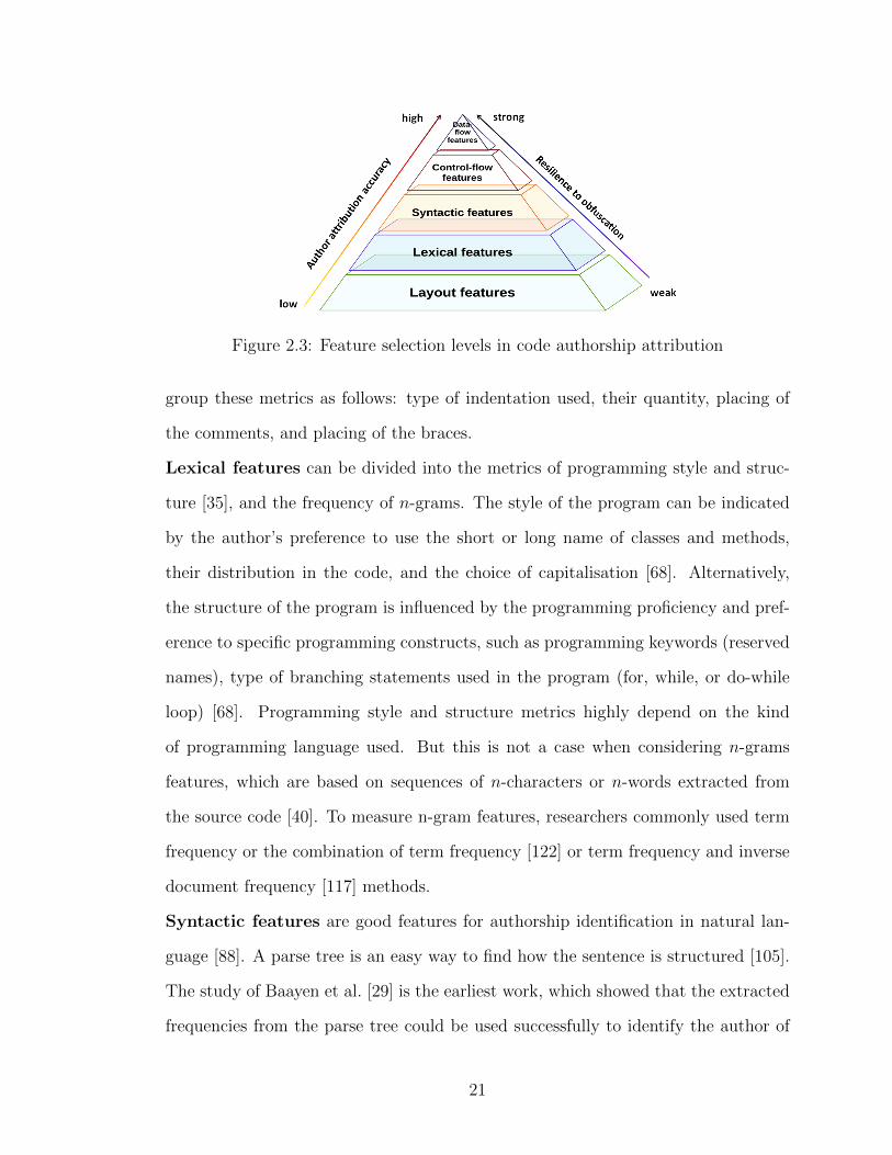
Figure 2.3: Feature selection levels in code authorship attribution
group these metrics as follows: type of indentation used, their quantity, placing of
the comments, and placing of the braces.
Lexical features can be divided into the metrics of programming style and struc-
ture [35], and the frequency of n-grams. The style of the program can be indicated
by the author’s preference to use the short or long name of classes and methods,
their distribution in the code, and the choice of capitalisation [68]. Alternatively,
the structure of the program is influenced by the programming proficiency and pref-
erence to specific programming constructs, such as programming keywords (reserved
names), type of branching statements used in the program (for, while, or do-while
loop) [68]. Programming style and structure metrics highly depend on the kind
of programming language used. But this is not a case when considering n-grams
features, which are based on sequences of n-characters or n-words extracted from
the source code [40]. To measure n-gram features, researchers commonly used term
frequency or the combination of term frequency [122] or term frequency and inverse
document frequency [117] methods.
Syntactic features are good features for authorship identification in natural lan-
guage [88]. A parse tree is an easy way to find how the sentence is structured [105].
The study of Baayen et al. [29] is the earliest work, which showed that the extracted
frequencies from the parse tree could be used successfully to identify the author of
21

the document.
Lately, the features extracted from the abstract syntax tree (AST) of the code have
shown, that they can be successfully applied to source code authorship [44, 28].
These features represent the code structure and resistant to the changes in the code
layout; moreover, they often describe properties, such as code length, nesting levels,
and branching [44]. AST does not include layout elements, such as unessential punc-
tuation and delimiters (braces, semicolons, parentheses, etc.). Caliskan et al. [44, 45]
investigated syntactic features to indentify the authors of the C/C++ source code
samples. The authors published the Code Stylometry Feature Set, which includes
layout, lexical, and syntactic features. These features showed a high accuracy–
97.67%, 96.83%, and 94% to identity the author of the code among 62, 250, and 1, 600
candidate authors, respectively. Lately, the study of Alsulami et al. [28] showed the
possibility of automatically extraction of the syntactic features from the AST using
artificial recurrent neural network architectures, such as Long Short-Term Memory
(LSTM) and Bidirectional Long Short-Term Memory (BiLSTM).
Control-flow features have been used in binary code attribution [26] and are not
typical for source code attribution. These features are derived from a control-flow
graph (CFG) that represents the sequence of the code statements execution and
their possible branching [143]. The nodes of the control-flow graph composed by
code statements, which are linked by directed edges to show the sequence of code
statements execution [143]. In binary authorship analysis graphlets (subgraphs of
the control-flow graph) and supergraphlets (extracted by combining adjacent nodes
of the control-flow graph) can be employed to de-anonymize the author of the binary
code [26].
Data-flow features may be used to identify the author’s coding style through the
preference of employed algorithms and specific data structures used in the code [143].
These features are derived from the program dependence graph (PDG) that deter-
22

mines data and control dependences for each statement and predicate in a pro-
gram [143]. It was introduced by Ferrante et al. [65] and it was originally used for
program slicing [139]. In binary authorship analysis, Alrabaee et al. [26] used API
data structures for this task. For binary code representation, authors analysed the
dependence between the different registers that are often accessed regardless of the
complexity of functions.
The arrows in Figure 2.3 represent our systematization of the influence of feature
selection on attribution accuracy and their strength of obfuscation. Layout features
are related to the layout of programs, therefore these features are weak and easily
modifiable, for instance, they can be changed by a code beautifier and code for-
matter [55]. Lexical features also correspond to the layout of code, however, these
features are more difficult to modify [55]. Layout and lexical features alone are still
less accurate (67.2% by [55]), than when used in combination with syntactic features
(92.83% by [44]). Most of these features do not survive the compilation process.
On the other hand, control-flow and data-flow features that retain programming
proficiency are considered to provide stronger evidence of a developer’s style.
2.2 Summary
In this chapter, we covered an introduction to authorship attribution work, which
was necessary for understanding this thesis work. The comprehensive review of the
related work showed a spectrum of representations, features, and models for code
authorship attribution, which proved a diversity of solutions in code authorship
attribution. However, over the years, these studies had also revealed a number of
challenges that the area faces:
Lack of datasets Research in code authorship attribution suffered from a lack of
open-benchmark datasets. Researchers had to collect software for specific authors
23

manually. Using privately received data (e.g., students’ assignments) hindered repro-
ducibility of the experiments. Open data sources (public repositories and textbook
examples) raised questions about the sole authorship and context of considered code.
Code received from programming competitions did not reflect natural coding habits
due to the artificial and constrained nature of competition setup.
Lack of consensus of appropriate data characteristics for code attribution
Answering the questions regarding the suitable data characteristics is essential for
the code attribution domain and could have implications for both accuracy and
performance of attribution techniques in the deployment environment. Within this
context it is necessary to understand whether the results obtained by previous studies
were due to optimal or perhaps coincidental matches between data and approach or
due to the attribution technique’s tolerance to dataset imperfections.
24

Chapter 3
Adversarial code attribution
Existing authorship attribution research assumes that authors are honest and do not
attempt to disguise their coding style. We challenge this underlying assumption and
explore existing authorship methodologies in adversarial settings.
We propose to create an attack on current authorship attribution techniques (Sec-
tion 3.1). This attack identifies a developer (the victim) and transforms the attacker’s
source code to a version that mimics the victim’s coding style while retaining the
functionality of the original code. We referred to this attack as author imitation
attack.
To subvert an author imitation attack, in Section 3.2, we introduce a novel coding
style obfuscation approach called author obfuscation. The idea of author obfuscation
is to allow authors to preserve the readability of their source code while removing
identifying stylistic features that can be leveraged for code attribution. Unlike ex-
isting obfuscation tools which work towards concealing the specific details in the
program (data structures and algorithms, the logic of the program, keys and pass-
words) [33], the author obfuscation approach obscures the coding style of developers.
The coding style transformations used for author imitation and author obfuscation
are described in Section 3.3.
25

3.1 Author imitation attack
The majority of previous studies show that we can successfully identify a software
developer of a program. The question that naturally arises from this situation is
whether it is possible to mimic someone else’s coding style to avoid being detected
as an author of their software. In other words, can we pretend to be someone else?
Consider the following scenario: Alice is an open-source software developer. She
contributes to different projects and typically stores her code on the GitHub reposi-
tory. Bob is a professional exploit developer who wants to hide his illegal activities
and implicate Alice. To do this, he collects samples of Alice’s code and mimics her
coding style. An example of Bob’s malware ends up in the hands of a law enforce-
ment agency, where the analysis shows that the malware is written by Alice. This
unfortunate scenario is possible due to the recent advances in the code authorship
attribution field that focuses on the identification of the developer’s style.
Author imitation attack aims at deceiving existing authorship attribution techniques.
The flow of the attack is shown in Figure 3.1 and includes three steps: (1) collect-
ing the victim’s source code samples, (2) recognizing the victim’s coding style, and
(3) imitating the victim’s coding style. The pseudocode for this attack is given in
Algorithm 3.1.
The attack starts with identifying a victim and retrieving samples of his/her source
code Vs = (s1, s2, ..., sn). Typically, authors of open-source software hide their iden-
tity through nicknames and avatars. However, many GitHub accounts leave a per-
sonal developer’s information open, essentially allowing an attacker targeting a par-
ticular person to collect the victim’s source code samples.
Once the samples are collected, the second step is to analyse them and identify the
victim’s coding style. The coding style of the victim is represented by a vector of
features. The strategy is to apply a set of coding style transformations Mi,j(A) to the
set of attacker’s source code samples A = (t1, t2, ..., tk) until the difference between
26

Figure 3.1: An overview of author imitation attack
the original victim style V and the modified attacker style is negligible.
The set of coding style transformations Mi,j is defined on the major feature levels i
given in Figure 2.3, e.g., layout (i = 1), lexical (i = 2), syntactic (i = 3), control-
flow (i = 4), and data-flow (i = 5). The particular transformation j for each of
the feature levels can vary. An example set of possible transformations is given in
Table 5.3.
The distance between the feature vector extracted from the original source code
of victim V and the feature vector derived from the modified source code of A is
determined based on cosine similarity1. Such a metric is widely implemented in
information retrieval that models data as a vector of features and measures the
similarity between vectors based on cosine value.
Definition 3.1.1 (Cosine similarity for author imitation attack). In authorship at-
tribution, source code can be represented as a vector of features whose dimension p
1For our analysis we experimented with a variety of similarity measures including Euclideandistance, Cosine distance, Minkowski distance, Jaccard distance, and Manhattan distance. SinceCosine similarity outperformed all other metrics, we employ it in our work.
27

depends on the considered feature set. A feature’s value can refer to term frequency,
average, log, or anything else depending on the characteristics used.
Let ~sn =−−−−−−−−−−−−→(sn,1, sn,2, ..., sn,p) denote the feature vector of the n-th source code of victim
V , and let ~tk =−−−−−−−−−−−→(tk,1, tk,2, ..., tk,p) denote the feature vector of the k-th source code of
attacker A, where sn,h and tk,h with h ∈−−−→(1, p) are float numbers indicating the value
of a particular feature. The cosine similarity between ~sn and ~tk is defined as follows:
CosSim(~sn, ~tk) = ~sn·~tk|| ~sn||·||~tk||
=
√∑ph=1 sn,h·tk,h√∑p
h=1(sn,h)2·√∑p
h=1(tk,h)2
The similarity is measured in the range 0 to 1. CosSim = 1 if two vectors are
similar, CosSim = 0 if two vectors are different.
The code transformations Mi,j that produce the maximum similarity, i.e.,
CosSim(Vs,Mi,j(At))→ max, are the ones that the attacker should use to transform
the original code in order to obtain a semantically equivalent code that mimics the
victim’s coding style. Note that these transformations should be calculated once per
victim and can be applied to any of the attacker’s programs.
Finally, to imitate the victim V , the attacker recursively applies the transformations
identified in the previous step to A∗, i.e., Im(V,A∗) = Mi,ji(A∗).
Complexity The attack described in Algorithm 3.1 consists of a precomputation
step and the main phase. In the precomputation step the algorithm searches for the
code transformations that once applied to the attacker’s source code samples and
transforms the attacker’s coding style into the victim’s coding style. The complexity
of this step depends on the number of specific transformations defined for each of
the five feature levels. It should be noted that these transformations only need
to be determined once per victim. The main phase consists of applying selected
transformations to an attacker’s source code. The time complexity of this phase
grows linearly as the size of the attacker’s code increases.
28

Algorithm 3.1 Author imitation attack
Input: Vs = (s1, s2, ..., sn) -victim’s source code samples;At = (t1, t2, ..., tk) -attacker’s source code samples;A∗ = (m1,m2, ...,ml) -attacker’s any source codes
Output: Im(V,A∗) -attacker’s source codes A∗ with imitated victim’s V coding style# precomputation partfor all i = 1 to 5 do
for all j doapply transformation Mij to each At
compute θ(i, j) =∑s
∑t
CosSim( ~Vs, ~Mij(At))
end fortake j such that θ(i, j) is maximum
end forreturn pairs (i, ji)
5i=1 and their correspondent transformations Mi, ji
# main partfor all A∗ doapply i transformations Mi, ji to attacker’s source code A∗ recursively: Im(V,A∗) = Mi,ji(A
∗),
where Mi,ji(A∗) is a recursive function, such as: ˜Mi+2,ji+2
(A∗) = ˜Mi+1,ji+1(Mi,ji(A
∗))end forreturn Im(V,A∗)
3.2 Author obfuscation
To subvert an author imitation attack, we propose a method that manipulates the
source code to hide an author’s coding style while preserving code readability. The
goal of author obfuscation is to prevent its detection by authorship attribution sys-
tems.
The author imitation attack applies transformations to the attacker’s source code
to imitate the victim’s style. The most effective imitation can be generated when
the distance between the source code feature vector of the victim and the modified
source code feature vector of the attacker is negligible, i.e., transformations produce
the maximum similarity between the two vectors.
Intuitively, to make an author imitation attack unsuccessful, we should convert the
original author’s style to a more generic, less personalized version of it, while fully
retaining the functionality of the code. These transformations should produce mini-
mal similarity between the feature vector of the original and modified author source
code. The pseudocode of author obfuscation is given in Algorithm 3.2.
29

Algorithm 3.2 Author obfuscation
Input: Vs = (s1, s2, ..., sn)– author’s V source code samples;V ∗ = (v1, v2, ..., vn)– code, which author V wants to hide
Output: Hide(V ∗)– source code without author’s V style# precomputationfor all i = 1 to 5 do
for all j doapply transformation Mij to each Vs
compute θ(i, j) =∑s
CosSim( ~Vs, ~Mij(Vs))
end fortake j such that θ(i, j) minimum
end forreturn pairs (i, ji)
5i=1 and their correspondent transformations Mi, ji
# obfuscationfor all V ∗ doapply i transformations Mi, ji to author’s source code V ∗ recursively: Hide(V ∗) = Mi,ji(V
∗),
where Mi,ji(V∗) is a recursive function, such as: ˜Mi+2,ji+2(V ∗) = ˜Mi+1,ji+1 (Mi,ji(V
∗))end forreturn Hide(V ∗)
3.3 Coding style transformations
Current code transformations, common in software development, typically aim to
disguise the appearance of the code, making it difficult to understand and reverse
engineer the obfuscated software. In contrast, the proposed coding style transforma-
tions remove the original author’s style, but leave the source code visible, readable,
and understandable.
In this work, we look at transformations at the layout, lexical, syntactic, control-flow,
and data-flow levels.
The code examples for several control-flow and data-flow transformations were taken
from the work of Banescu et al. [32] and Ertaul et al. [61]; these examples were
modified according to our needs.
3.3.1 Layout transformations
Comments Comments are a high indicator of a programmer’s coding style. De-
velopers usually use line comments or block comments [56]. Block comments bound
30

a part of source code which can be multiple lines or a part of a single line. This
part is framed with a start separator and an end separator [136]. Line comments
begin with a start separator and proceed to the end of the line [21]. In C, C++,
and Java languages, the separator of block comments is ”/∗” and ”∗/” and line com-
ments are separated by ”//”. Java has additional Javadoc comments which are block
comments, but are separated by ”/∗∗” and ”∗/”. This comment is explicitly created
to be understandable to the Javadoc processor [14]. In addition to this, Ding et al.
defined ”comment lines as pure comment lines, non-comment lines include lines with
inline comments” [55]. In this work, to hide the style of comments we identified dif-
ferent comment transformations: change all comments to Block comments, or Line
comments, or Javadoc comments. To remove any developer’s traits in comments
we are using the following transformations: Delete all inline comments, Delete all
pure comment lines, and Delete all comments. To confuse the attribution system,
the following transformations are used: Add pure comments on each line, Add in-
line comments on each line, and Add pure comments on each line and one inline
comment.
Curly brackets Several works in code authorship attribution identified that the
placement of curly brackets used in code exhibits variations of an individual’s coding
style [71, 130]. There are many bracket and indent styles programmers use, as it also
formats program source code and influences code readability [107]. The diversity
of styles of brackets can be identified by taking a closer look of their placement
around the compound statement ”{...}”, which usually follows by control statements
(”while”, ”for”, ”if”, ”else-if”, ”do”, etc.) [9].
Figure 3.2 shows the variety of curly brackets styles used in programming languages.
For example, the K & R (i.e., Kernighan and Ritchie) style is commonly utilized
in C and C++. This style, used in the original Unix kernel, was first mentioned in
Kernighan and Ritchie’s book [86]. Every function has its open and closed brackets
31

Figure 3.2: Curly brackets styles
at the following line and have the same indentation as its defined function, although
blocks inside a function use the same line to place curly brackets [10].
The following ”One True Brace Style” and Linux style are variants of the K & R
brackets style [9]. The main difference is that the ”One True Brace Style” style
uses additional curly brackets to separate one line conditional statements. However,
the Linux style utilizes tabs for indentation [12]. The Linux kernel developer, Linus
Torvalds, created the Linux brackets style. A detailed description of such style is
available at the Linux kernel coding standard [11].
The Stroustrup style uses the Linux style, although the open curly brackets are on
the next line from function definitions only and the open curly brackets are on the
same line as everything else [16]. The creator of the Stroustrup style was Bjarne
Stroustrup, who was a developer of C++ language, and the description of this style
first appeared in his book [129].
The Mozilla style uses Linux brackets. Open brackets are on the next line in classes,
structures, enumerations, and function definitions, but the brackets are attached
to everything else, including namespaces, arrays, and statements within a function.
32

The Mozilla style was created mainly for use in Mozilla codebase and was described
in the Mozilla coding style standard [13].
The Whitesmiths, along with the Allman and the VTK styles put the curly brackets
connected to a control statement on the next line. However, these styles use different
methods of indentation. The Allman style has the same indentation as the control
statements [2]. The statements bounded by Whitesmiths brackets have the same in-
dentation as the curly bracket [23]. And the VTK has indented brackets, except for
the open brackets of classes, arrays, structures, enumerations, and function defini-
tions. Also, the origin and use of these brackets are not the same. The Whitesmiths
style was well-known in the first versions of operating system Windows [23]. This
style was initially described in the Windows programming book [59]. The Allman
style was named after a computer programmer Eric Allman and was used by Pascal
languages [1]. The VTK style was inspired mainly by such open-source software
projects like VTK or ITK and was described in the ITK coding convention [22].
The GNU style uses brackets on the next lines similar to the Allman style, although
the entire block is indented, not just the curly brackets. This style was strongly
suggested by the GNU Coding Standards, therefore mostly all developers followed
it in the GNU project software [6]. The Horstmann style is also a variation of the
Allman style, as it has open and closed brackets on the next line, but the first block
statement is placed on the same line as the open curly bracket [8]. The Horstmann
style was used first by Cay S. Horstmann in his book [82].
The following Java, Banner, Lisp styles have the open bracket, when the line is ended
and when the compound statement is started [14]. Although the closed bracket of
the Java and the Banner styles should be placed at the beginning of the line and
have the same indentation as compound statement [14], the closed bracket of the Lisp
style is attached to the last statement. The Google coding style is similar to the Java
style, but with an indent of 2 spaces. The origin and the use of such bracket styles
33

are the following. The Java style is used in the Oracle (formerly Sun Microsystem)
style guide [14] and a large part of the Java API source code follows this style [9].
The Banner style has sometimes been termed Ratliff style [93], which is named after
C. Wayne Ratliff, the creator of the database program Vulcan. The Lisp style is
very common in Lisp code and its specification is available at the Common Lisp
Style Convention [3]. The Google style is used in Google’s coding standard [7].
The Pico style is the most rarely used brackets style; this style is mostly followed by
Pico language designers [9]. Such a style saves space with a line of code, as it uses
attached closed brackets.
Indentation A significant number of early programs utilized tab characters to
indent. Unix editors mostly use tabs equal to eight characters, although Windows
and iOS operating systems use four [9]. Current source code editors can utilize any
size of indentation; moreover, they can use a combination of spaces and tabs [18].
As a result, quantity and type of indentation depend highly on the programmer’s
choice. Furthermore, the use of spaces or tabs is a divisive debate in the developers
community [18]. A majority of developers have the opinion that tabs in comparison
with spaces decrease cross-platform portability, therefore should not be used [146].
The writers of the WordPress coding standards have a different opinion, stating that
tabs increase portability [24].
In this research work we are using not only different styles of indentation but they are
mixed, for example, Indent using tabs for indentation and spaces for line alignment.
We also varied the placement of the indentation in the code. For example, we are
inserting space padding around parenthesis On both sides, or Only on the outside, or
Only on the inside. Also we inserted space padding After only commas or Around
operators. The expressions in ”if”, ”for”, and ”while” statements can be separated
by blank spaces. We are using the following transformations to remove indentation:
Remove all space or tabs padding and Remove extra space padding around parenthesis.
34

Lines Programmers usually use blank or empty lines to enhance the readability
of source code by dividing the program into logical-related sections [145]. Java
Code Convention stated that ”two blank lines should always be used between class
definitions and sections of source code, and one blank line between methods, local
variables in the method, and block” [14]. However, not all developers are following
these rules and therefore are revealing their coding style. To hide their traits we use
the following transformations: Delete all empty lines within a function or method,
Delete all empty lines, and Add empty line after each nonempty line.
The difference in coding style can also be indicated by counting the number of
statements and declarations per line. Some programmers use several declarations
on the line, although one statement per line is encouraged by the Oracle Coding
Standard [14] since it helps to comment the code. We noticed the same situation with
statements, therefore, the following transformations are used:Write each statement
in one line, Write several statements in one line, Write one declaration per line, and
Write several declarations in one line.
3.3.2 Lexical transformations
Lexical transformations, such as identifier renaming is an essential aspect of code
obfuscation. Authors of programs like to choose identifier names at their discretion.
As a result, identifier renaming can hide such characteristics and make authorship
attribution much harder.
Names Most commercial obfuscators use a renaming transformation that uses
short identifiers, for example, a single character. As the obfuscator reads the code,
it selects the next trivial identifier for replacement. Such simple renaming transfor-
mation is hard to reverse. Although the program logic does not change, the names
are hard to read, making it challenging to understand the code.
35

In this research work, we also look at name transformations for long names, instead
of short, as such names can also mislead attribution systems. We used English
dictionaries to hide the names of variables, classes, and methods.
Not only can the whole name reveal the authors of the code, but also the specific
patterns used by authors, such as, if the first letter is uppercase or lowercase, or if
the particular characters, i.e., a dollarsign or an underscore, were used. We are using
different transformations to hide such features.
3.3.3 Syntactic transformations
Syntactic transformation works by hiding the coding style of the programmer from
properties extracted from abstract syntax trees. The study of Caliskan et al. [45]
showed that adding syntactic features is a reliable indicator of a developer’s traits.
AST leaves The tree node can represent either a root node, a branch node, or
a leaf node [20]. The non-leaf nodes indicate program’s operators, when the leaf
nodes indicate mostly operands [99]. Operands are variables or expressions, which
are used in operators to evaluate the expression. AST never contains layout details,
such as commas, parentheses, and semicolons. AST leaves can be obfuscated by
name transformations. Also for imitating the author style, all comments from the
imitated author can be copied and inserted, as AST leaves do not reveal the format
of comments (like layout features), but their content.
AST nodes Each node in an AST is an instance of an AST class, for example,
”IfStmt”, ”AssignStmt”, ”AddExpr”, and ”VarDecl”. To change such classes, we use
straightforward techniques, such as changing ”for” loops to ”while” loops, and chang-
ing ”else-if” to ”switch-case”. With such transformations, the depth and frequency
of each node are changed.
36

3.3.4 Control-flow transformations
Control-flow transformations works by hiding the initial control-flow of the program
by ”reordering and obfuscating the execution paths and structure of the original
program” [134]. Such transformations can target logic, predicates, aggregation, and
ordering.
Logic One of the transformations which aim to hide the logic of the code is control-
flow flattening [134]. Chenxi Wang first introduced this technique in her thesis [137].
Such transformation rearranges basic blocks in the code (e.g., method body, loops,
and conditional branch instructions), so it seems, that they share the same group
of successors and predecessors [98]. Figure 3.3 presents the example of the function
obfuscated by control-flow flattening. A variable ”next”, used in ”switch” state-
ment, specify the sequence, which the multiple ”case” should be followed by, then
the statements inside of ”case” are executed until a ”break” statement is reached
out [32]. In Control-flow flattening with ”switch” dispatch, each block becomes a
”case” in a ”switch” statement, and the ”switch” is wrapped inside an infinite loop.
Alternatively, in Control-flow flattening with ”go-to” dispatch, direct ”go-to” is used
to jump between blocks instead of ”switch-case”.
Control-flow flattening transformations vary not only by type of dispatch used (”switch-
case” or ”go-to”), but also by the complexity of used conditional branches. For
example, Control-flow flattening with normal branch uses normal branches, such as
if (a > b) go − to L1 else go − to L2. Another option is to compute the condi-
tional branches, such as x = (a > b); go − to expression over x, which is used in
Control-flow flattening with compute branch.
37

Figure 3.3: Control-flow flattening transformations (with ”switch” and normal dispatch)
38

Opaque predicates A predicate is a conditional expression, which is mainly cre-
ated from well-known algebraic theorems. For instance, predicate (x3 − x ≡ 0(
mod 3)) is opaquely true for all integers x, and x2 < 0 is always false for any integer
x. These predicates are invariant as it always evaluates to the same value for all
possible inputs.
Such transformations were first introduced by Collberg et al.; they proposed to split
the control-flow by ”adding conditional jumps based on opaque predicates” [47].
During program execution, the predicate’s assessment follows in a conditional jump
to the initial source code [47]. The authors also suggested adding dead code for
making deobfuscation more complex.
The traditional approach to constructing the opaque predicates is to create additional
branches in the control-flow graph. If opaque predicates take only true value for any
variable, the part of the program which corresponds to the opaque’s execution to
false value will be skipped by the program [62]. As a result, random functions can
be inserted. These kinds of transformations are called Opaque predicates with call to
RandomFunction(), when false and presented on the left side of Figure 3.4. Instead
of random functions, a non-existing function can be inserted in the place of junk
code [62]. In this case, such a transformation is called Opaque predicates with a call
to NonExistingFunction, when false. Another variation is Opaque predicates with a
call to existing function when true when the branch to false is not used at all.
Different ways to obfuscate a code by opaque predicates is to define a predicate,
which takes false and true values randomly, then run the identical program using
both branches. Although, it should be combined with another transformation that
can make the two identical programs extremely hard to find as these programs are
equal [62]. These transformations are called Opaque predicates with question. Fig-
ure 3.4 shows different kinds of opaque predicate transformations.
39

Figure 3.4: Opaque predicate transformations
Aggregation The transformations based on control aggregation ”break up compu-
tations that logically belong together or merge computations that do not” [47]. Merg-
ing of methods can be produced, for example, by generating much bigger methods
that have a lot of variables inside, these variables may not always be depended [32].
Banescu et al. [32] in their work provided an example of function merging and func-
tion splitting. Listing 3.1 shows Function merging. The function f3 is the result of
merging functions f1 and f2. Taking into account that function f3 uses additional
variable c, this variable affects the execution time of f1 and function f2 functions.
For example, when this variable take an even value, the program runs function f1,
but when this variable takes an odd value, the program runs the function f2 [32].
Rugaber et al. [118] presented ideas for implementing function merging and called
this interleaved code.
Listing 3.2 shows Function splitting. This transformation splits one function f3 into
two small f1 and f2 functions. This transformation modifies the the program’s
control-flow, breaking the initial structure written by developers.
40

Listing 3.1: Function merging example
1 f1 ( i n t a1 , i n t a2 ) {
2 k=4;
3 i f ( a1<3)
4 k=k+6;
5 k∗=a2 ;
6 }
7
8 f2 ( i n t a1 , i n t a3 ) {
9 m=a1+12;
10 m=m/a3 ;
11 }
Listing 3.2: Function splitting example
1 f3 ( i n t a1 , i n t a2 , i n t a3 ){
2 i f ( a3 % 2==0) {
3 k=4;
4 i f ( a1<3)
5 k=k+6;
6 k∗=a2 ;
7 } e l s e {
8 m=a2+12
9 m=m/a2 ;
10 }
11 }
Ordering Programmers put related parts of code close together. Placement (local-
ization) of such elements can help a reverse engineer to see what parts of code belong
together. Pappas et al. [106] first introduce function argument randomization. There
are two main variants of such transformation: Function argument reorder, which ran-
domizes the order of arguments of the function and Function argument reorder with
adding bogus arguments, which randomizes and adds extra bogus arguments.
The purpose of such transformations is to hide common functions’ signatures. Or-
dering can be implemented easily for software without any external dependencies
(for example, libraries) [32]. However, if this transformation is applied to a library,
then it modifies that library and all programs which are referenced to this library
should be updated.
3.3.5 Data-flow transformations
Data-flow transformations ”change the representation and location of constant val-
ues” [32], such as strings and numbers, which are embedded in the application, also
these transformations modify the constant values in the memory.
Numeric Literals Integer and string literals are the most common data type
in most programs, and for that reason, it is crucial to obfuscate them. However,
41

transformation of numeric literals can result in decreasing the execution time, in
contrast to simple operations on integers or string literals, which were initially used
by programmers.
One of the transformations which aim to obfuscate integers is Integer obfuscation
using opaque expressions. Such transformation was first introduced by Collberg et
al. [49]. This transformation is focused on hiding constants by creating expres-
sions dependent on external variables. Such variables are called opaque expressions;
the difference between opaque expressions and opaque predicates (used in control-
flow transformations) is that the first one has a non-boolean, constant value during
program execution, although, opaque predicates can be boolean, i.e., false or true.
Banescu et al. [32] showed that the constant value 1 in the program (Listing 3.3)
can be obfuscated using the opaque expression cos2(x) + sin2(x). The example of
obfuscated code is shown in Listing 3.4.
Listing 3.3: Original code example
1 in t main ( ) {
2 in t m = 1 ;
3 // do smth
4 return 0 ;
5 }
Listing 3.4: After integer obfuscation
1 in t main ( ) {
2 double a = s in ( a to f ( av [ 1 ] ) ) ;
3 double b = cos ( a to f ( av [ 1 ] ) ) ;
4 i n t m = ( in t ) ( a ∗ a + b ∗ b ) ;
5 // do smth
6 return 0 ;
7 }
The transformation of literal strings can be conducted by the transformation, which
is called String obfuscation using string generation function [19]. Literal data usually
has a lot of useful information that reveals trade secrets or passwords. One of the
ways to obfuscate such information can be done by turning this data into a code
that generates such data (i.e., string) at execution time [48].
Another way is to transform the literal strings of the source code in ciphertext using
a monoalphabetic substitution cipher like Affine Cipher [61]. Such transformations
were first introduced by Ertaul et al. [61]. They substituted every character in the
string with another character in the alphabet. For instance, the authors showed that
42

string ”Caser” can be encrypted as ”Igykx” where ”C” substitutes for ”I”, ”a” for
”g”, etc. The example of their transformation is presented in Listing 3.6, where it
pushes string forward by a random number of characters.
Listing 3.5: Original code example
1 in t main ( ) {
2 St r ing l a b e l = ”Caser ” ;
3 p r i n t l n ( ”Before ” + l ab e l ) ;
4 }
Listing 3.6: After string obfuscation
1 in t main ( ) {
2 St r ing l a b e l =f1 ( l abe l , random label ) ;
3 p r i n t l n ( ”Before ” + l ab e l ) ;
4 St r ing method f1 ( St r ing labe l , i n t m) {
5 }
Data Encoded integer variables changes the data representation of variables. One
of the main purposes of such transformation is not to disclose an initial value of the
integer variable [19].
One of the ways to achieve this is by Variable obfuscation using linear transformation,
which was created by Farrugia et al. [64]. For instance, the work by Banescu et
al. [32] showed how to obfuscate a variable k using the following transformation:
k′ = v ∗k+w with integers w and v, which are randomly selected. Listing 3.7 shows
the example of original program with integer variables: m, n, and l. The example of
obfuscated program is shown in Listing 3.8, where m, n, and l are encoded by using
liner transformation from the work of Banescu et al. [32].
Listing 3.7: Original code example
1 in t main ( ) {
2 in t var1 = . . .
3 i n t var2 = . . .
4 i n t m = var1 ;
5 i n t n = var2 ;
6 i n t l = m∗n ;
7 p r i n t f ( y ) ;
8 }
Listing 3.8: After variable obfuscation
1 in t main ( ) {
2 in t var1 = . . .
3 i n t var2 = . . .
4 i n t m = 1789355803 ∗ var1 + 1391591831;
5 i n t n = 1789355803 ∗ var2 + 1391591831;
6 i n t l = ((3537017619 ∗ (m ∗ n) − 3670706997 ∗ m)−
7 −3670706997 ∗ n) + 3171898074;
8 p r i n t f (−757949677 ∗ y − 3670706997) ;
9 }
Arithmetic Arithmetic transformations work by replacing statements, which con-
tain arithmetic and boolean operations, by statements with operations, which are
43

more complicated and difficult to read and understand [32]. Such obfuscation was
initially created by Zhou et al. [148]. This transformation is called Arithmetic obfus-
cation using boolean expressions. Banescu et al. [32] provided the example of original
code with simple addition expression: d = a + b + c (presented in Listing 3.9) and
wrote it another way by using more complex boolean and arithmetic expressions
(shown in Listing 3.10).
Listing 3.9: Original code example
1 in t main ( ) {
2 in t a = a to i ( av [ 1 ] ) ;
3 i n t b = ato i ( av [ 2 ] ) ;
4 i n t c = a to i ( av [ 3 ] ) ;
5 i n t d = a + b + c ;
6 return 0 ;
7 }
Listing 3.10: After arithmetic obfusca-
tion
1 in t main ( ) {
2 in t a = a to i ( av [ 1 ] ) ;
3 i n t b = a to i ( av [ 2 ] ) ;
4 i n t c = a to i ( av [ 3 ] ) ;
5 i n t d = ( ( ( a ˆ b) + ( ( a & b) << 1) ) | c ) +
6 +((( a ˆ b) + ( ( a & b) << 1) ) & c ) ;
7 return 0 ;
8 }
3.4 Summary
This chapter explored the potential of current authorship attribution techniques to
be deceived. We introduced an author imitation attack to imitate the developers
coding style in the open-source software repositories.
To resist this attack, we developed the author obfuscation approach and proposed
coding style transformations, which could hide the coding style of a software author.
The evaluation of the author imitation attack and the proposed obfuscation trans-
formations are presented in Chapter 5.
44

Chapter 4
Assessing effects of dataset
characteristics on attribution
performance
To validate our author imitation attack and author obfuscation technique, which
were proposed in the previous chapter, we need an appropriate and suitable dataset.
Through many studies that have documented the experiments aimed at studying
the effectiveness of code attribution, one question remained common: what is the
most appropriate dataset required for attribution of any code. Since no benchmark
datasets are available in this field, researchers resorted to using ad hoc data that
retained at least some characteristics of programming practices, e.g., archives of
students’ programming assignments [92, 73, 60], programs written by textbook au-
thors [133], programming competition archives [44, 28, 125], and open-source repos-
itories [78, 147, 30, 124].
Such data diversity in experimentation creates some concerns. Using privately col-
lected data (e.g., students’ assignments) hinders reproducibility of the experiments.
Open data sources (public repositories and textbook examples) raise questions about
45

the sole authorship and context of considered code. Code received from program-
ming competitions does not reflect natural coding habits due to the artificial and
constrained nature of competition setup.
Beyond the concerns about the source of data, these datasets vary drastically in the
number of analysed authors, samples, length of the code and even quality of code,
making a comparative analysis of studies challenging. For example, MacDonell et
al. [96] experimented with seven authors in the dataset obtaining 88% accuracy in
attribution. McKnight et al. [103] achieved 66% with 525 authors. Both Tennyson
et al. [133] and Caliskan et al. [44] obtained 98% accuracy while experimenting with
200 samples and nine samples per author, respectively. Dauber et al. [54] showed
that it is possible to attribute code snippets (with 70% accuracy) that have only a
few lines of code, while the majority of studies find it necessary to experiment with
lengthy code.
Such ad hoc approaches to data selection naturally raise questions regarding the
appropriate data characteristics for code attribution:
• How much data is enough to demonstrate the effectiveness of an attribution
method? In other words, what are the suitable data characteristics, such as
a number of authors, samples per author, and length of samples necessary for
the code attribution task?
• Are these characteristics dependent on the data source, data quality, and con-
text? In other words, would these data characteristics be appropriate for
data retrieved from different environments, i.e., source code from GitHub vs.
GoogleCodeJam repository?
• Finally, what is the effect on the accuracy of code attribution if appropriate
characteristics are not selected?
The concerns regarding appropriate data characteristics are not new. The Burrows et
46

al. [42] study was one of the first to question the quality and variability of data. A few
other researchers also brought up potential effects of data bias on study results [54,
128, 104, 45].
Answering the questions regarding appropriate data characteristics is essential for
the code attribution domain and may have implications for both accuracy and per-
formance of attribution techniques in the deployment environment. Within this
context, it is necessary to understand whether the results obtained by previous stud-
ies were due to optimal or perhaps coincidental matches between data and approach
or due to an attribution technique’s tolerance to dataset imperfections. This is one
of the focuses of our work.
We approach these questions by first analysing data employed by the existing studies
in the area of source code attribution and replicating their experiments. We proceed
with exploring the effect of common code, examining source code size, samples size,
and author set size effects on attribution accuracy. Finally, based on our findings,
we develop a balanced large-scale authorship attribution dataset and offer it to the
research community.
4.1 Replication study
Given the considerable variability of data characteristics of the 21 reviewed studies
(Table 2.1), it is beneficial to bring these studies to a common denominator. We
begin our analysis by replicating these studies.
Data To ensure the validity of our analysis, we requested the original datasets em-
ployed by these studies. Out of the 27 datasets from the 21 reviewed studies we
were able to collect 7 datasets. These datasets, however, provide a sufficient rep-
resentation of experimental data quality used in the field. For example, MacDonell
et al.’s [96] data contains the smallest number of authors (7), and data provided
47

by Dauber et al. [54] has source code with only a few lines of code (samples with
one line). Data used by Caliskan et al. [44] has the smallest number of samples per
author (9), while McKnight et al.’s [103] set has the largest number of authors (525).
These seven datasets were derived from three different sources: GitHub repository,
GoogleCodeJam competition, and textbook programming assignments. For discus-
sion purposes, in the rest of this work, we will refer to the datasets from these studies
by the first name of the author, e.g., ’McKnight dataset’ will refer to data from [96]
work.
Features The majority of the reviewed studies claim to offer unique sets of features
capable of capturing developers’ stylistic traits. Since the accuracy of attribution
changes drastically depending on the study, we aim to explore what features are
sufficient for attribution and the extent of their contribution to the final result. We
analyse features concerning four significant groups: numeric features extracted from
layout and lexical levels, n-gram features, and syntactic features extracted from AST.
For our analysis, we select three feature sets that were the most prominent in the
history of source code attribution and are often seen as benchmark features.
The first studies in the code authorship attribution were primarily experimenting
with numeric features extracted from layout and lexical levels. The study by Krsul
et al. [92] was first to publish 49 metrics for C/C++ language. MacDonell et al. [96]
and Gray et al. [75] further improved them by using ANOVA test to measure features’
significance. Ding et al. [55] combined and adapted these metrics for Java language.
Although the authors never provided the final subset in the original study, this was
corrected by the follow-up study by Burrows et al. [42] which derived a final feature
set of 56 metrics from the original Ding et al. [55] study. Lange et al. [94], Gull et
al. [78], Elenbogen et al. [60], and Yang et al. [144] also experimented with Ding et
al. [55] features in their works. In this replication analysis, we use Ding et al. [55]
feature set derived by Burrows et al. [42] study.
48

Throughout the evolution of work within the attribution domain, n-grams features
have attracted a lot of research interest due to their simplicity and generally good
performance [41]. Kothari et al. [91] in their study featured a set of n-grams that was
later leveraged by other researchers, e.g., Bandara et al. [30], Shevertalov et al. [124],
Franzeskou et al. [73], Tennyson et al. [133], and Zhang et al. [147]. As such we add
Kothari et al.’s [91] feature set to our analysis.
The final feature set that we selected for experiments is a set derived by Caliskan
et al.’s [44] study. This set contains syntactic features derived from AST along with
some layout and lexical features. Dauber et al. [54], Simko et al. [125], and McKnight
et al. [103] used these features in their studies. Wisse et al. [142] leveraged the large
portion of Caliskan et al.’s [44] features in their analysis, adding additional features
applicable for Javascript language.
To summarize, we use three prominent feature sets for evaluation: Ding et al. [55],
Kothari et al. [91], and Caliskan et al.’s [44] sets. In the rest of this work, we will
refer to these sets as Ding, Kothari, and Caliskan feature sets.
4.1.1 Experimental setup
This section covers the details of various tools and techniques, which were used
for our evaluation of the dataset characteristics (Chapter 4) and proposed attacks
(Chapter 5).
Our experiments were performed using a desktop with Ubuntu 16.04.3 64-bit. Our
hardware had 32 GB random-access memory. The model name of our Intel processor
was Intel(R) Core(TM) i7-3770 CPU clocked at 3.40GHz.
To promote research in the area of code authorship attribution, we release the soft-
ware, which was written and the software, which was used for the tasks mentioned
below (i.e., data extraction and cleaning, code parsing, feature extraction, classifi-
cation, coding style transformations, and metrics evaluation). They are available at
49

Github 1.
Data extraction In this work, for extracting the data from GitHub we used the
GitHub data API 2, and a search method 3, which allowed us to apply different
filters to the results (for example, number of contributors). Although it is chal-
lenging to guarantee sole authorship of any code posted online, we took reasonable
precautions by filtering repositories marked as forks, as these are typically copies
of other authors’ repositories and do not constitute original work. An additional
check for multiple-author repositories was performed by examining the commit logs.
Repositories with logs containing more than one unique name and email address
combination (potentially indicating the involvement of several authors) were also
excluded. To remove duplicated and shared libraries, we further excluded programs
with duplicate hashes and code from ’lib’ and ’ext’ folders. For grouping the data
by code size and programming language, we used Cloc software 4. For extracting
the data from GoogleCodeJam, we used the GoogleCodeJam API 5, implemented
in Java by Caliskan et al. 6 The code for extracting data from GitHub was written
by undergraduate student Celine Perley with a help of software developer Nguyen
Cong Van during her internship in our lab. The assistance with finding appropriate
methods and techniques to solve this task was provided by me.
Data cleaning To remove similarity from datasets, we used MOSS similarity anal-
ysis tool 7. All the results from running MOSS script is shown on their website and
can be analysed there. When this analysis becomes complicated (for example, due to
the amount of analysed data) additional code and scripts for extracting and analysing
1https://github.com/alinamatyukhina/Attribution Real World/2https://developer.github.com/v3/3https://developer.github.com/v3/search/4http://cloc.sourceforge.net/5https://github.com/Faylixe/googlecodejam-client6https://github.com/calaylin/CodeStylometry/tree/master/Corpus7https://theory.stanford.edu/ aiken/moss/
50

these data were written by me.
Code parsing At first source code should be parsed to determine the meaning of
each string in the code. For parsing Java language, we used Javaparser library 8 and
the code, which was written by Celine Perley. For parsing the C and C++ code, we
used code analysis platform Joern 9, Gremlin graph traversal language 10 and the
software by Caliskan et al. 11.
Feature extraction The software for extracting Ding, Caliskan, Kothari, and
improved features were written by me. The code for extracting Caliskan features
outputs the following feature vectors separately, which were helpful for our feature
analysis: term frequency AST node bigrams, term frequency of word unigrams in
source code, term frequency of keywords, term frequency of AST node type exclud-
ing leaves, term frequency of code unigrams in AST leaves, term frequency inverse
document frequency of code unigrams in AST leaves, etc. The codes for extracting
byte and token n-gram features with different n size were written by me too.
Classification The previous approaches to source code authorship attribution em-
ploy various classification algorithms for attribution analysis while not providing
much justification for their algorithm’s selection. Caliskan et al. [44] utilized Ran-
dom Forest classifier, Burrows et al. [42] used Naive Bayes, Decision Tree, k-nearest
neighbor classification, neural network, regression analysis, support vector machine,
and voting feature interval.
For our classification, we used the implementation of machine learning algorithms
by the Weka 3.8.2 platform [79]. We used four common machine learning classifiers
including Naive Bayes (NaiveBayes), Random Forest (RandomForest), J48 decision
8http://javaparser.org/9http://mlsec.org/joern/
10https://github.com/tinkerpop/gremlin/wiki/11https://github.com/calaylin/CodeStylometry/
51

tree implementation of ID3 (J48), and IBk implementation of the k-nearest neighbor
algorithm (IBk). Since Burrows et al. [42] retained default parameters, for proper
comparison we followed the same practice and did not maintain configuration for
NaiveBayes, J48, and IBk. For the RandomForest algorithm, we chose 300 as the
number of trees following the configuration used by Caliskan et al. [44].
For avoiding the problem of over-fitting, we used k-fold cross-validation, where k is
the number of samples in the dataset. If the dataset contains less than ten samples
per author, we set k to the minimum number of samples per author. With ten or
more samples per author, we used ten-fold cross-validation, a common practice in
machine learning research [89].
Coding style transformations Our layout, lexical, and syntactic transforma-
tions, which we defined in Section 3.3, were made using Artistic Style 3.1 12, a
popular formatter from open-source platform SourceForge 13. The control-flow and
data-flow transformations were made using Tigress 2.2 14. Tigress is a code-to-code
obfuscator created by Collberg et al. The output of the obfuscated program is C
source code. For compilation, we used gcc 5.4.0. Renaming obfuscation for C was
made by Stunnix 15. Control-flow transformations for Java language were written
by Omar Hussein during his summer project in our lab. The assistance with finding
appropriate methods and techniques to solve this task was provided by me.
Metrics evaluation For evaluation of the proposed coding style transformations,
we used various metrics, which we described in more detail in Section 5.4. Some
of these metrics, for example, program complexity and nesting level were calculated
by using a freeware program SourceMonitor 16. The software for finding Halstead’s
12http://astyle.sourceforge.net/astyle.html/13https://sourceforge.net/14http://tigress.cs.arizona.edu/15http://www.stunnix.com/prod/cxxo/16http://www.campwoodsw.com/sourcemonitor.html
52

program length and readability were written by me. Execution time was calculated
by me using the clock() function for C language and System.nanoTime() for Java
language.
4.1.2 Evaluation
Table 4.1 shows the results of our replication analysis. None of the feature sets
can adapt to the changes in data which essentially indicates that in a deployment
setting none of the techniques produce expected results. Although the accuracy
of attribution with every feature set varies significantly among datasets, Kothari
features show the most consistent performance, while Caliskan features show the
highest accuracy.
Interestingly, all feature sets showed the lowest (or the second lowest performance)
on McKnight dataset, which has the largest number of authors (525), and Dauber
data, which has the code samples with the smallest length (4.9 LOC on average).
Both of these datasets [103, 54] were extracted from the Github repository as opposed
to other sets that were generated from other sources (except for [144]). This naturally
brings up a question of how the data from GitHub is different from other sources.
On the other hand, both Caliskan and Simko features were originally tested on
GoogleCodeJam data. Simko et al. [125] used a smaller subset of Caliskan dataset
set with only 50 instead of 250 authors, yet more samples per author (16 samples
on average [125], compared to 9 in [44]). Although the original study indicated
the scalability of Caliskan feature set to a varying number of authors, our analysis
showed degradation in performance (from 98.04% to 84.5%).
4.1.3 Dataset analysis
We look further into the characteristics of datasets to understand what might have
influenced the results of our analysis.
53

Table 4.1: The results of replication study
Name of dataset Original result Caliskan etal.’s [44] fea-tures
Ding etal.’s [55]features
Kothari etal.’s [91]features
Yang et al.’s [144] dataset 91.1% 89.88% 65.49% 86.32%Dauber et al.’s [54] dataset 70% 69.02% 44.6% 65.2%Caliskan et al.’s [44] dataset 98.04% 98.04% 78.3% 91.2%McKnight et al.’s [103] dataset 66.76% 62.99% 54.6% 63.4%Tennyson et al.’s [131] dataset 98.2% 92.14% 90.69% 90.32%MacDonell et al.’s [131] dataset 88% 99.7% 73.23% 84.15%Simko et al.’s [125] dataset 84.5% 84.5% 72.5% 79.01%
Typically, the data extracted from original data sources are cleaned and processed for
further analysis. This cleaning commonly includes removal of third-party data, in-
cluding shared libraries and duplicate code. The existence of such third-party code is
considered noise that might make the attribution process more challenging [103]. In-
deed, third-party libraries are typically shared among software programs, and there-
fore, exhibit a different coding style that might confuse the attribution process.
On the other hand, duplicate code samples belonging to the same authors introduce
bias in classification and make the attribution task easier. The situation becomes
more interesting when code samples are not identical, but slightly different (we refer
to it as common code). This often happens with code reuse, i.e., software developers
commonly reuse code previously written by them or in some instances by others. To
understand the influence of duplicate and common code on authorship attribution
accuracy, we explore its presence in all seven datasets.
Our analysis showed the presence of duplicate code samples only in one of the
datasets. Dauber dataset contained 9.72% of dublicate files. For our further analysis,
all these duplicates were removed.
To measure the similarity between programs in datasets we used the MOSS tech-
nique [17] that employs a robust winnowing algorithm to select a subset of the token
hashes as the document fingerprints [123]. Using these fingerprints, MOSS measures
a percentage of mutual overlap between two programs.
54

The percentage of mutual overlap within authors in datasets varied significantly. To
guide further analysis, we define a mutual overlap threshold, taken as a lower bound
of the value of mutual overlap measured by MOSS. If two programs of the same
author have more mutual overlap than a defined threshold, we remove one of them
from the dataset. As such, the conservative approach is to set the limit to 0%, then
no overlap is tolerated, and all code needs to be distinct. The other extreme is to
establish a threshold at 100%. This effectively requires removing all identical files
while allowing smaller amounts (less than 100%) of code overlap within individual
programs.
Figure 4.1 shows the correspondence between mutual overlap threshold and percent-
age of samples being detected as having common code, and therefore being removed
from the dataset. As the analysis shows, MacDonell dataset contains more duplicate
files than any other dataset, i.e., nearly 5% of programs were detected with 100%
overlap. Tennyson and Caliskan datasets included approximately 1% of duplicate
samples.
As our previous results in Table 4.1 show, we achieve the lowest accuracy results on
Dauber and McKnight datasets. Both datasets are outliers compared to other sets
and represent extreme cases. The code from Dauber set has the smallest code size–
only a few lines– while McKnight dataset contains the largest number of authors,
compared with other datasets (525).
55
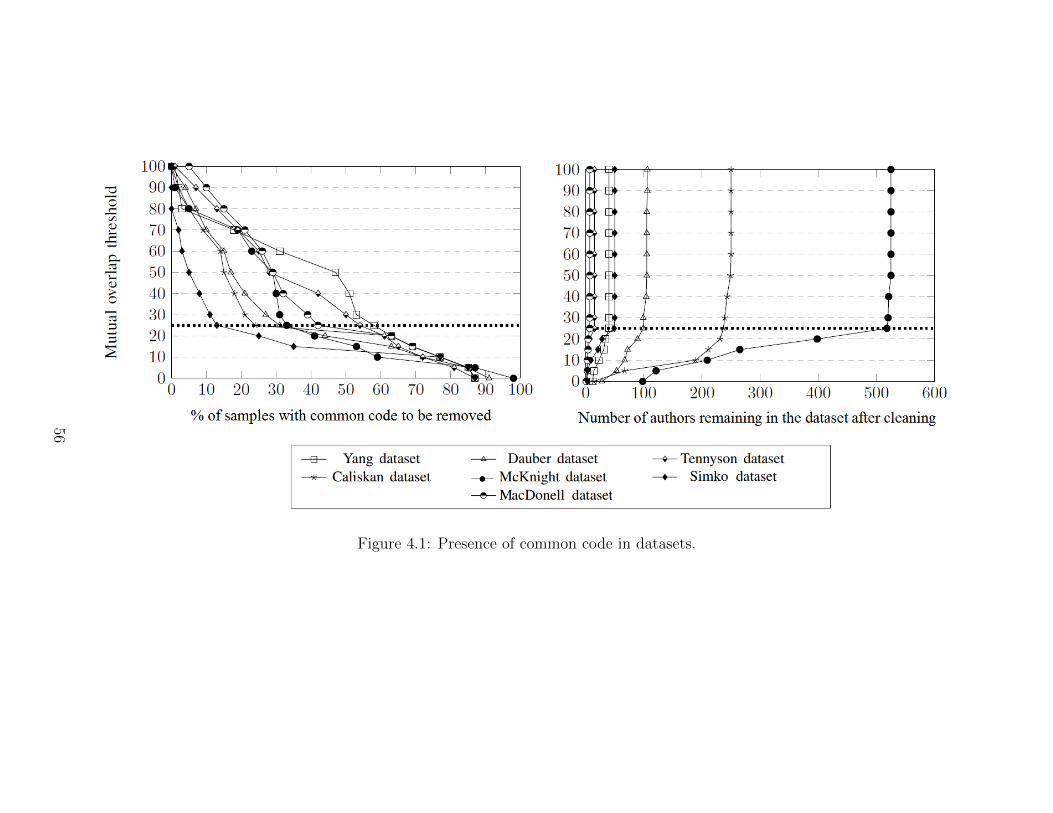
Figure 4.1: Presence of common code in datasets.
56

Table 4.2: Accuracy of attribution after removing common code
Name of dataset % ofcom-moncode* inoriginaldata
Standarddevia-tion inoriginaldata
N ofauthorsaftercleaning
Av. Nof sam-ples/authoraftercleaning
Totalfilesaftercleaning
Caliskanetal.’s [44]features
Ding etal.’s [55]features
Kotharietal.’s [91]features
Yang et al.’s [144] dataset 57.58% 18.43 40 30 1282 61.21% 41.57% 59.33%Dauber et al.’s [54] dataset 30.96% 12.35 99 104 10977 53.81% 31.2% 49.6%Caliskan et al.’s [44] dataset 23.91% 44.6 237 7 1712 85.12% 65.4% 80.3%McKnight et al.’s [103] dataset 32.95% 19.46 518 40 846 48% 40.2% 49.5%Tennyson et al.’s [131] dataset 54.3% 29.46 15 93 3305 68.19% 63.21% 65.39%MacDonell et al.’s [131] dataset 41.88% 25.23 7 29 204 81.35% 53.67% 69.23%Simko et al.’s [125] dataset 12.5% 45.63 49 14 704 79.78% 67.24% 72.29%*Results were obtained with mutual overlap threshold25%
Dauber dataset shows 0% of duplicate files within the author’s code. This result
indicates that perhaps Dauber dataset was cleaned of duplicates within individual
authors and but not between authors.
At 70% threshold, MacDonell dataset has the highest percent of common code (21%).
With thresholds between 50% to 30%, Yang dataset has the highest amount of
common code (around 50%). Setting up a threshold at 10% removes from 60% to
75% of programs in all datasets. The overall trend is somewhat expected, i.e., the
lower the threshold (less tolerance toward common code), the more programs should
be removed.
To balance the amount of data available for analysis with common data, we further
assess a number of unique authors that are retained in the set after removing the
programs with common code. Figure 4.1 shows the number of authors remaining in
the datasets with respect to mutual overlap threshold. At 20% threshold most of the
datasets start losing authors, McKnight set shows the most drastic loss, i.e., from
525 to 400 authors. To balance between the number of remaining authors and the
amount of common code, we decided to use 25% as a final mutual overlap threshold.
Table 4.2 lists the datasets with the corresponding amount of remaining common
code with the selected threshold of 25%.
Table 4.2 also shows the existing amount of variation in common code present in the
57

datasets. The standard deviation of common code is largest in Caliskan (44.6) and
Simko datasets (45.63). Note that both datasets were extracted from GoogleCode-
Jam repository. The smallest deviation is observed in Yang, Dauber, and McKnight
datasets. Although these sets are extracted from GitHub, they are not overlapping
and as such indicate that the amount of common code present in GitHub is somewhat
consistent across different authors’ repositories.
The major impact of removing programs with duplicate code from these datasets
is seen in a number of samples per author, i.e., Yang dataset decreased from 72 to
30 samples on average, Tennyson dataset decreased from 203 to 93, and MacDonell
dataset from 50 to 29.
Consequently, the reduction of common code resulted in a significant decrease in
overall attribution accuracy. Yang and Tennyson datasets showed nearly 30% drop
in accuracy after removal of common code (57.58% and 54.3%, respectively). The
attribution accuracy on other datasets also decreased by 15% - 20%, with a removal
of 20% to 40% of common code. The only dataset that did not show a significant
change in accuracy is Simko dataset. This is expected as the dataset contains the
least amount of common code (12.5%), therefore removing it only results in 5%
change.
Furthermore, Figure 4.2 shows how the attribution result of datasets gradually de-
creases as common code being removed from datasets. Our results show that the
existence of common code in datasets influences the attribution accuracy. The more
substantial presence of common code in dataset, the more significant differences in
attribution accuracy it brings. For example, removal of nearly 50% of the com-
mon code in a dataset leads close to 25% decrease in attribution accuracy; if the
dataset has 30% of the common code, its removal leads to 15% drop in accuracy.
These results clearly show that removal of only identical code (which is a common
practice) is not sufficient. Further similarity analysis of code is a necessary step to
58

0 10 20 30 40 50 60 70 80 90 1000
102030405060708090
100
Common code (%)
Acc
ura
cy
Yang datasetDauber datasetCaliskan dataset
McKnight datasetTennyson datasetMacDonell dataset
Simko dataset
Figure 4.2: The changes in accuracy with respect to the amount of common code
understand how attribution technique can potentially perform in various deployment
environments.
4.1.4 Correlation analysis of features from previous studies
In addition to variability in accuracy, three feature sets differ significantly in the
number of features.
Ding et al. [55] used discriminant analysis to identify 56 best performing features.
Kothari et al. [91] selected 50 top features. In both studies, number of features is
constant and does not depend on the size of data. In contrast, Caliskan et al. [44]
offered a very diverse set of features that depending on the analyzed data can grow
exponentially. None of the studies offered a clear analysis of selected features and
rationale for their selection. Some features, e.g., term frequency (TF) of AST node
types and term frequency-inverse document frequency (TFIDF) of AST node types
in [44], seem to be co-dependent.
As such we analyze the correlation of features in these three feature sets by calculat-
ing Pearson’s correlation coefficient ρ. The correlation coefficient ranges from −1 to
1. According to our calculations, the coefficient ρ of all Ding and Kothari features
ranges from −0.1 to 0. These values indicate that both feature sets contain only
59

Name of features Name of features ρ Number of featuresASTNodeTypesTF ASTNodeTypesTFIDF 0.99 81ASTNodeTypesTF ASTNodeTypeAvgDep 0.1 81ASTNodeTypesTFIDF ASTNodeTypeAvgDep 0.1 81CodeInASTLeavesTF CodeInASTLeavesTFIDF 0.99 135698CodeInASTLeavesTF CodeInASTLeavesAvgDep 0.04 135698CodeInASTLeaves TFIDF CodeInASTLeavesAvgDep 0.04 135698numkeyword from cppKeywords ln(numkeyword/length) 0.97 7
Table 4.3: Correlation coefficient analysis for Caliskan features
linear independent features.
The correlation coefficients of Caliskan features show a different picture. While the
majority of features are linearly independent (ρ = 0), some of the features appear to
be highly correlated. Table 4.3 shows Pearson’s correlation coefficient between dif-
ferent groups of Caliskan features. For example, ρ = 0.99 between ASTNodeTypesTF
and ASTNodeTypesTFIDF, and CodeInASTLeavesTF and CodeInASTLeavesTFIDF.
Typically, the researchers consider only TFIDF measurements to prevent bias be-
tween authors with many samples and authors with a few samples [114, 90].
High correlation, ρ = 0.97 also exists between numkeyword from cppKeywords and
ln(numkeyword/length), as both features essentially contain the same set of keywords
(e.g., do, else-if, if, else, switch, for or while).
Further analysis of code unigrams of AST leaves revealed some duplication with
word unigrams. Indeed, consider an example given in Figure 4.3. Many of the
word level unigrams extracted directly from source code appear in the leaves of
AST and consequently are included in unigrams of AST leaves. To avoid a po-
tential bias by introducing duplicative features, we removed ASTNodeTypesTFIDF,
CodeInASTLeavesTFIDF, and numkeyword from cppKeywords features.
Finally, we measured the performance of Caliskan feature set after removing elements
with high-correlation (ρ is between 0.5 and 1.0, and between −0.5 and −1.0), i.e.,
ASTNodeTypesTFIDF, CodeInASTLeavesTFIDF, numkeyword features. We refer
to this new feature set as Caliskan uncorrelated features. Overall, the number of
features in this uncorrelated feature set decreased by 19.6%.
60

Figure 4.3: Example of source code and its AST
Name of features Number of features AccuracyCaliskan features 691562 74.4%Caliskan uncorrelated features 555776 74.4%
Table 4.4: Accuracy with uncorrelated features (401 plus 75 authors dataset)
Table 4.4 shows that there is no difference in attribution accuracy between using an
original or uncorrelated feature set despite a reduction in the number of features.
4.2 Impact of dataset characteristics on the per-
formance
The replication study, although it revealed shortcomings of experimental datasets,
did not address the questions of appropriate data characteristics for consistent at-
tribution analysis. For this analysis, we create an independent dataset by collecting
samples of Java source code from the GitHub dataset.
As opposed to the limited amount of data in the GoogleCodeJam dataset, GitHub
contains near 67 million total repositories. The data from GitHub can be grouped
and sorted by lines of code, number of samples per author, number of authors, etc.
The programs in GitHub are typically more complex, including third-party libraries,
61

use source code from other authors and focus on solving diverse tasks (e.g., from
game development to middleware). As we saw in the replication study, performing
authorship attribution on data retrieved from GitHub data is more challenging.
We collected programs in April 2018 by using Github. Following our previous analy-
sis, we also removed all source code samples that contained more than 25% of mutual
overlap for every author. After this cleaning, authors that remained with less than
10 samples per author were removed as well. Our final dataset consisted of 2056
authors with 47,288 source code programs with LOC range 1-1692, and 352 LOC in
average, number of samples with range 10 to 337, and 46 files per author on average.
We offer our dataset to the research community in the hope of diversifying and
strengthening experiments in this field 17.
4.2.1 How long should code samples be?
The length of code samples employed in previous studies ranged significantly. For
example, Burrows et al. [41] used programs varying from 1 to 10,789 lines of code,
Tennyson et al. [133] took samples ranging from 1 to 3265 lines, Frantzeskou et
al. [73] worked with samples that fluctuated in size from 36 to 258 lines of code. In
forensics, where often only small source code snippets are available, a performance
of traditional approaches tends to be less accurate [54].
Whether these results were coincidental or a direct result of a smaller number of
lines in considered code samples is not clear. Our analysis showed that Dauber’s
data were highly redundant and not equally distributed, i.e., 3125 programs were
one-line samples, 2171 had from 2 to 9 lines, 445 programs had from 10-99 lines, and
34 samples had from 100 to 554 lines.
For a fine-grained view, we group our data by code size into the following subsets: 1 to
50 lines of code (LOC), 51 to 100 LOC, 101 to 200 LOC, 201 to 300 LOC, 301 to 400
17https://github.com/alinamatyukhina/Attribution Real World
62

Table 4.5: The datasets grouped by LOC
Name of dataset Number ofauthors
Number offiles
Min #samplesper author
Average# samplesper author
1 to 50 LOC 1059 39996 10 38
51 to 100 LOC 520 24783 10 47
101 to 200 LOC 384 23026 10 59
201 to 300 LOC 171 7790 10 45
301 to 400 LOC 86 3889 10 45
401 plus LOC 75 3423 10 44
LOC, and 401 plus LOC. Table 4.5 shows the statistics of these subsets. Although
the largest of these subsets contained 1059 authors, the smallest collection only has
75 authors. To ensure consistency in experimentation, for each of these subsets (with
exception of the last one 401 plus LOC ) we take 5 random selections of 75 authors.
The reported results are the averaged scores across these 26 experiments. Since the
number of lines in code varies, we fix the number of samples per author for each
collection at 10.
0 100 200 300 400 500 600 700 8000
10
20
30
40
50
60
70
80
90
100
Number of lines in code
Acc
ura
cy
Ding featuresCaliskan featuresKothari features
Figure 4.4: Accuracy vs LOC
Figure 4.4 shows the correspondence between the size of code samples and the accu-
racy of attribution. The results allow us to draw three important conclusions. First,
the general trend in the accuracy of code attribution is similar across all features
sets. The large code samples’ size does not directly translate to better accuracy. The
63

accuracy increases substantially between the sizes if 1-50 LOC and 101-200 LOC,
which in itself is not surprising as the larger programs provide a better view of the
developer’s coding style. However, after that point the performance plateaus and
does not significantly increase, except for Ding features that dived slightly from 38%
to 33% using 301 to 400 LOC data. Thus, when the data are scarce, having an
option of using smaller code samples (100-200 LOC) with little impact on accuracy
is beneficial.
The second aspect of these results relates to the small code snippets. With the 1
to 50 LOC dataset we were able to reach most 52% accuracy with Caliskan features,
24.4% with Ding features, and 37.87% with Kothari features.
Finally, it is clear that Caliskan feature set outperforms the other two approaches
regardless of code size.
4.2.2 How many samples per author are needed?
Since authorship attribution aims to derive a developer’s coding style, having suffi-
cient data for this analysis becomes essential. The number of samples used in attri-
bution domain across the years varied significantly from 3 [94] and 9 samples [44] to
28-128 [30], and 1,360 - 7,900 samples per author [109]. In most cases, the selection
of programs per author is driven by data availability. Thus, the question of how
many samples per author are needed for analysis remains. We looked into this ques-
tion through generating 6 collections containing 5, 10, 20, 30, 40, and 50 samples
per author for every code size: 1 to 50 LOC, 51 to 100 LOC, 101 to 200 LOC, 201
to 300 LOC, 301 to 400 LOC, and 401 plus LOC. Since both code size and number
of samples per author vary, we set the number of authors for each collection to 50
(the maximum number possible to maintain consistency across all collections). As a
result, we continue our experiments with 36 datasets. For 5 samples per author we
use 5 cross-validation, for the rest 10 cross-validation.
64

Figure 4.5 demonstrates the results of our experiments. The accuracy of attribution
drastically decreases with a limited availability (less than 10 samples) of samples per
author. With only 5 samples per author, results vary between 22.5% and 36.1% with
Ding features, 51.37% and 69.2% with Caliskan features; and 15.32% and 65.18%
with Kothari features. This experiment clarifies two important points. First, the
variations in accuracy beyond 20 samples per author decreases (less than 11% for
Dings features, 6% for Caliskan features, and 7% for Kothari features). Since the
number of authors in this experiment was fixed, we further explore relationship
between varying number of authors and samples in Subsection 4.2.3.
The second important outcome of this experiment is that this variability in accuracy
cannot be compensated by the size of code samples unless the number of samples per
author is limited (less than 10). For example, for 5 samples per author we obtained
51.37% with 1 to 50 LOC, while with 301 to 400 LOC we obtained 69.2% (Caliskan
features).
Finally, irrespective of code size, the accuracy does not increase with the increase
of a number of samples per author. The accuracy plateaued for all feature sets for
over 20 samples per author.
Kothari features showed the largest gap in performance with 5 samples per author
data (15.32% for 1 to 50 LOC to 65.18% for 201 to 300 LOC ). The explanation
of this behavior stems from the nature of the employed features. Since this feature
set is comprised of mostly n-grams, having longer code (or more samples) allows
capturing the author’s coding style more effectively.
Overall, the best performance was achieved with Kothari features (90.78%), with
Caliskan set closely following behind (86.76%).
65

Figure 4.5: The impact of varying number of samples per author
Figure 4.6: The impact of varying number of authors on accuracy
66
4.2.3 How many authors are needed?
Traditionally, author attribution techniques have been applied to closed world prob-
lems (e.g., plagiarism detection), i.e., given a small set of known authors, the goal is
to identify one that has authored a document. With the advances in attribution do-
main, this is a relatively simple task that in most cases can be reliably and accurately
solved [44].
As the pool of authors increases, this task becomes more difficult. Individual author
style has to be unique enough to consistently distinguish itself from a large number
of other potential authors. In this context, previously mentioned questions (code
length and number of author’s samples) become more prominent.
In previous research, the smallest number of authors (2) was used by Pellin et
al. [109]. The majority of the studies in the field generally have up to 20 au-
thors [96, 73, 91, 30, 41, 78, 91, 60, 133, 124, 94]. The higher number of authors is
less common, i.e, 29 - 70 authors were used in [92, 55, 73, 142, 144, 28, 125, 147],
106 authors in [54] and 525 authors in [103].
The large-scale authorship attribution analysis was explored only by Caliskan et
al. [44]. Their analysis reached 98% accuracy with a 250 author set, and 93% ac-
curacy with 1,600 authors. However, a follow-up study by Simko et al. [125] that
mirrored [44] methodology on the same dataset for 5, 20, and 50 authors received
different result - 100%, 88.2%, and 84.5%, respectively.
In this work, we explore the impact of a varying number of authors with a varied
length of code and number of samples. The majority of studies in authorship at-
tribution use less than 70 candidate authors. Following this practice, we randomly
select 2, 10, 20, 30, 40, 50, 60 and 75 authors from our larger sets of authors. All
reported results are averaged values obtained from 5 runs with random selections of
authors to improve reliability. For the first set of experiments, we fixed the number
of samples per author to 10.
67

Figure 4.6 shows the effect of the author set size in authorship attribution. The
results unanimously show that attributing a code between two authors is straight
forward in most cases. All three attribution features sets were able to achieve 100%
accuracy. This result was dependent on the code size. With Ding features perfect
accuracy was obtained with 201 to 300 LOC dataset, smaller code 1 to 50 LOC was
only attributed with 73.2% accuracy.
On the other hand, features of Caliskan and Kothari performed better with a shorter
code of 1 to 50 LOC (100% accuracy) than with longer code 201 to 300 LOC (90%).
Such difference stems in part from the nature of the employed features. Caliskan
feature set primarily includes the unigrams that can be captured even with the short
code. On the other hand, Ding feature set contains more layout features that can be
more accurately extracted from a longer code.
A visible common trend across all three feature sets is a steep decline in performance
with an increase in the number of authors in the analysis. With 30 authors in dataset
attribution, for example, can be done with an accuracy of 57.41% with Ding features,
82.33% Caliskan features and 83.12% Kothari features (201 to 300 LOC ). Attribution
of 40 to 75 authors is challenging. The best performance for 75 candidate authors
was obtained with Caliskan features on 401 plus LOC dataset (74.4%). The code of
401 plus LOC can be performed with an accuracy of 44.13%, 74.4%, and 62.4% with
Ding, Caliskan, and Kothari features.
The smaller code sizes exacerbate the problem. With more than 20 authors in the
dataset, Ding features only achieve the accuracy of around 30% (1 to 50 LOC ), and
around 45% (51 to 100 LOC ). With Kothari features the accuracy falls to 40% with
more than 50 authors (1 to 50 LOC ). Caliskan features are slightly more tolerant to
a large number of authors even with smaller code sizes (53.2% with 1 to 50 LOC ).
Overall, these experiments allow us to point out two aspects. First, attributing
a small number of authors is straightforward, while attributing a large number of
68

authors (above 40-50 authors) is challenging for all feature sets which is contrary to
other reported results. Second, longer code samples although theoretically retain
more information about coding style do not offer a significant benefit in attribution
of less than 50 authors. In the presence of over 50 authors, longer code samples allow
to boost performance. However, it is clear from our experiments that short code (less
than 200 LOC) is not suitable for attribution of data with over 50 authors. Third,
201 to 300 LOC set generally shows similar or better performance compared to sets
with longer code. One exception is attribution of 60 and above authors, where using
even longer code (400 LOC and above) provides a small increase of up to 5-8%. Still,
in most attribution scenarios there is no need for the longer code.
For the second set of experiments, we explored the relationship between the number
of authors and the number of samples per author. For this experiment, the number of
lines was fixed to 101 to 200 LOC. This set was chosen for two reasons. This number
of lines was most commonly used in other studies and our previous experiments
confirmed that this set generally shows an averaged performance among other LOC
sets.
For this experiment, we created 36 different collections with a varying number of
samples - 5, 10, 20, 30, 40, 50 for each author and number of authors- 2, 10, 30, 40,
50, 60, 75.
Figure 4.7 shows the accuracy of attribution with regards to the number of samples
and the number of authors. The results are similar to those obtained with varying
sample sizes (Figure 4.6). Attributing 2 authors even with only 5 samples is fairly
easy, yet, overall 5 samples do not allow the features to capture sufficient information
about the coding style. Interestingly, there is negligible difference in accuracy with
30-50 samples per author. This insight was also apparent from Figure 4.5 where
the accuracy value plateaued after 20-30 samples per author. In summary, in
attribution of over 20 authors 20-30 samples per author is sufficient. Increasing a
69

0 10 20 30 40 50 60 700
10
20
30
40
50
60
70
80
90
100
Number of authors
Acc
ura
cy
5 samples 10 samples 20 samples30 samples 40 samples 50 samples
Figure 4.7: Attribution accuracy with varying number of samples and number ofauthors on the example of Ding feature set
value of samples beyond 30 does not result in corresponding meaningful increase in
accuracy.
4.2.4 What features are the best?
Our analysis shows high variability in performance of three feature sets. This differ-
ence is in some aspects defined by the nature of the extracted features. To understand
the relationship between different types of features and accuracy of attribution anal-
ysis, we further explored the behavior of features under the varying size of code
samples and the number of authors.
Figure 4.8 shows the performance of Caliskan full feature set, TF unigram features,
and AST bigrams on sets with a varying number of authors and code samples’ sizes.
Along with the original Caliskan feature set, we consider two subsets extracted from
the full set: lexical TF unigrams and syntactic AST bigrams. TF unigrams are
interesting as they constitute almost 80% of the original Caliskan set. AST bigrams
70

Figure 4.8: Attribution accuracy of Caliskan features, TF unigram, and AST bigramson different LOC datasets
were chosen due to their potential accuracy that was reported to be nearly the same
as classification accuracy of the full Caliskan feature set [44].
As the results show, original feature set outperforms subsets except for several cases.
Attributing code between 2 authors is generally straightforward as we saw it in previ-
ous experiments, i.e., the performance of the original set is similar to the performance
of TF unigrams and varies slightly between 90% and 100% accuracy. Similarly, the
performance of original set and TF unigrams is almost identical with a few cases
that show an insignificant difference on long code samples (301 LOC and longer).
Syntactic AST bigrams’ performance is drastically different, i.e., it drops below 50%
in the attribution of 20 authors, and with 75 authors the accuracy does not increase
over 33.87% regardless of code size. It should be noted that original Caliskan et
al. [44] study reported 96.6% with 62 programmers on syntactic features claiming
superiority of AST bigrams.
AST features perform the worst with short code samples (1 to 50 LOC). This is
71

mostly due to the inability of small AST trees (that are created from short code
samples) to fully capture the syntactic patterns. As the size of the code increases,
we see an increase in performance. However, the scale of the growth will depend on
whether the code has enough to provide robust AST features. AST bigram features
capture the structural patterns of the code, so if the code is short, lacks conditional
statements or has many coding antipatterns such as ’spaghetti’ code, AST bigrams
will not adequately reflect the code style. On the other hand, good lexical features
(e.g., comments, names of methods/variables) have a significant contribution to an
increase in performance of attribution tasks.
As opposed to Caliskan et al. [44] work that focused on lexical word-unigrams fea-
tures, the study by Kothari et al. [91] employed byte-level n-grams. In their original
analysis, Kothari et al. showed that 4-grams outperform other n-gram sizes. The
question of the optimal size of n-grams has been also studied by other researchers.
For example, Frantzeskou et al. [73] showed that 6-grams and 7-grams perform the
best in byte-level n-grams. Burrows et al. [41] recommended that either 6-grams
of tokens or 14-grams of bytes as features should be chosen. Since none of these
studies ventured to provide a comprehensive analysis of n-gram features on different
datasets, we further investigate this aspect.
Figure 4.9 presents the performance of byte and token n-grams with respect to all
possible size of ’n’ on 1 to 50 LOC dataset. For these experiments, we fixed the
number of authors to 50 and the number of samples per author to 10. For this initial
experiment, we wanted to consider all possible n-grams, as the number of n-gram
features increases significantly with the increase of n, we chose the dataset with the
shortest code- 1 to 50 LOC. To identify the range of n-grams, which shows the best
performance, we fixed the number of authors to 50 and the number of samples to 10.
The analysis of code with the different number of samples and authors is discussed
later in Section 4.2.4.
72

Figure 4.9: Attribution accuracy with byte and token n-gram features on 1 to 50LOC dataset after information gain feature selection
The results show that byte n-grams outperform token n-grams when the size ranges
between 2 to 14. We obtained the best accuracy of 67.27% with byte level 3-grams
and 46.34% with token level 2-grams. With larger sizes of n-grams (above 15), we
can see that token n-gram gives higher accuracy than word n-gram, although the
efficiency of both features are much low on this section, with the best 17.04% of
token n-gram and 11.23% of byte n-gram. Generally, token n-grams show the steep
decrease in accuracy with increasing value of n, with the highest performance for
n = 1, 2. As opposed to this, the byte n-gram graph shows a sinusoidal decrease.
In general, it is believed that increasing value of n leads to a corresponding expo-
nential increase in the number of features [41]. This however is not always the case
and depends on the employed data. Figure 4.10 shows that the number of features
is increasing when n ranges from 1 to 10, after 10-gram the number of both byte
and token n-gram features are decreasing. The decrease of byte n-gram is much
steeper than decrease of token n-gram features. Figure 4.10 shows the number of
original n-gram features and their number after information gain feature selection.
For example, for n = 13 the number of features reaches 49,675 for token n-gram
and 42,599 for byte n-gram. After information gain feature selection, those numbers
73

Figure 4.10: Number of n-gram features before and after information gain featureselection on 1 to 50 LOC dataset
are 299 and 275, respectively. After information gain feature selection, the quantity
of tokens and bytes based features decreases to 0 for 80-gram, and for 130-gram,
respectively. As a result, the graphs on the Figure 4.9 are terminated when n equals
to 80 and 30, respectively.
Finally, we conducted multiple experiments to compare the performance of byte and
token n-gram features on various code sizes. As Figure 4.9 shows the steep decrease
of the attribution performance after 10-gram on both token and byte n-gram features.
As a result, in following experiments, we considered performance of n-grams in the
range between [1, 10]. The number of authors and the number of samples per author
were fixed to 75, and 10, respectively.
A number of interesting conclusions and issues concerning the effect of source code
size on n-gram features choice emerge. First of all, the results in Figure 4.11 indicate
that for all datasets (except 1-50 LOC), the best performing features among token
n-grams are 2-grams. After 2-grams attribution performance decreases. Our token
n-gram results contradict some conclusions of Burrows et al. [41] study. As we can
see token 6-grams are generally less accurate than 1 or 2-grams.
For values of n more than 3, byte n-grams significantly outperform token n-grams
for any code size.
74

Figure 4.11: Performance of byte and token n-gram features on datasets with differ-ent code size after information gain feature selection
75

0 10 20 30 40 50 60 700
10
20
30
40
50
60
70
80
90
100
Number of authors
Acc
ura
cy
1-gram 2-gram 3-gram 4-gram5-gram 6-gram 7-gram 8-gram9-gram 10-gram
Figure 4.12: Performance of byte n-gram features on a datasets with different numberof authors
Byte 3-grams give the best accuracy (57.2%) on datasets with limited code 1 to 50
LOC, although their performance increases to 78.4% on 201 to 300 LOC, and 73.6%
on 401 plus LOC. On code size of 301 to 400 LOC, byte 3-grams and 4-grams show
the same accuracy of 75.87%. Byte 4-grams outperform byte 3-gram features on
51 to 100 LOC, and 101 to 200 LOC, but the difference is negligible nearly 2%.
These findings contradict results reported in Frantzeskou et al. [73] study where the
authors indicated that 6-gram and 7-gram features perform worse than 3-grams and
4-grams. Such a difference in results can be explained by the type of data that was
used for analysis, i.e., Frantzeskou et al. [73] used academic and FreshMeat (OSS)
with a number of lines ranging from 23 to 980 in comparison to our GitHub dataset
with the fixed number of lines of code per every set.
Figure 4.12 and Figure 4.13 show the dependence of attribution accuracy on a number
of authors. The number of lines is fixed and equal to 1001 to 200 LOC. The worst
performing features are byte 1-grams on every dataset size, and the best performing
76
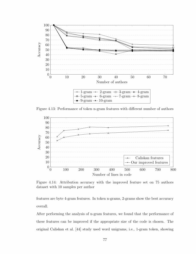
0 10 20 30 40 50 60 700
10
20
30
40
50
60
70
80
90
100
Number of authors
Acc
ura
cy
1-gram 2-gram 3-gram 4-gram5-gram 6-gram 7-gram 8-gram9-gram 10-gram
Figure 4.13: Performance of token n-gram features with different number of authors
0 100 200 300 400 500 600 700 8000
10
20
30
40
50
60
70
80
90
100
Number of lines in code
Acc
ura
cy
Caliskan featuresOur improved features
Figure 4.14: Attribution accuracy with the improved feature set on 75 authorsdataset with 10 samples per author
features are byte 4-gram features. In token n-grams, 2-grams show the best accuracy
overall.
After performing the analysis of n-gram features, we found that the performance of
these features can be improved if the appropriate size of the code is chosen. The
original Caliskan et al. [44] study used word unigrams, i.e., 1-gram token, showing
77

the high accuracy (Figure 4.4). We improved this result further by adding layout
features and choosing the best performing n-grams for given code size. Figure 4.14
shows that the accuracy of improved features increases on average by 10% on every
dataset.
Based on our experiments, we defined the optimal feature sets for datasets of various
sizes and offer them to the research community in the hope of strengthening exper-
iments (in Appendix A). We further use this feature set in the next section for the
evaluation of the author imitation attack and obfuscation techniques. We refer to it
as Our improved features.
4.3 Summary
Finding a proper dataset for an authorship attribution study is a challenging task.
Researchers often resort to using an available dataset with all its shortcomings. How
these shortcomings affect the results of attribution is not always clear.
In this chapter, we investigated how the quality of data impacts the overall per-
formance of authorship attribution. This is the first systematic study that offers a
practical insight into the performance of the existing attribution studies and looks
into the potential bias that different datasets’ shortcomings may bring.
From the series of experiments, we reached several important conclusions.
First and foremost, the presence of common code leads to an increase
in attribution accuracy. Our results showed that attribution on a dataset that
contains a high percentage of duplicate or similar code would lead to higher attri-
bution accuracy irrespective of dataset’s nature, size, and programming language.
We found that on average removing 50% of common code from dataset decreases
attribution accuracy by nearly 25%, while removal of 30% of common code brings
a 15% decrease. We feel that simple removal of duplicate code is not sufficient and
78

any study should undertake further analysis of code similarity. Although one may
argue that this is an obvious result, our research shows that many chose to ignore
this preprocessing step. We feel that it is essential to emphasize the degrading effect
of common and similar code on attribution task.
Second, attributing a large number of authors is challenging irrespective
of code size and the number of samples per author. Our experiments show
that it is straightforward to attribute a small number of authors for any attribution
approach (100% or nearly perfect accuracy depending on the selected feature set).
However, increasing the number of authors results in a significant deterioration in
performance. The most challenging is attribution of 40 and above authors. As such
an actual performance of an attribution method cannot be fully explored without
analysis of a full spectrum of authors including extreme cases of attributing 75 and
above authors.
Third, large code samples do not always translate to better accuracy. It is
challenging to accurately attribute small code snippets (1 to 50 LOC). The accuracy
however does not change significantly for programs containing 100 - 200 lines of code
and above. To the point that the difference in accuracy of attributing programs of
200-300 LOC and 401 LOC and above is negligible (in some cases less than 2%).
This is an important finding as having an option of using smaller code samples when
data is scarce is beneficial.
Fourth, increasing the number of samples per author does not always
result in a corresponding increase in accuracy even in attribution of large
number of authors. The accuracy of attribution in the presence of less than 10
samples depends on the size of available code, yet in attribution of over 20 authors
20-30 samples per author is sufficient. Increasing a value of samples beyond 30 does
not result in a corresponding meaningful increase in accuracy.
Fifth, a performance of token and byte n-gram features highly depends on
79

code size. For example, for short code we recommend using byte 3-grams, for code
from 51 to 200 LOC– byte 4-grams, and for large code from 201 LOC– byte 3-grams.
When the number of features is essential, we suggest using token 1-grams or 2-
grams, as they outperform byte n-gram features. We do not recommend considering
the values of n larger than 10, as the number of features increases exponentially with
a significant decrease in accuracy.
Based on our analysis and findings, we developed a balanced dataset and the optimal
feature sets for various code sizes. We offer these outcomes of our work to the research
community in an effort to strengthen code attribution field.
80

Chapter 5
Evaluation
This chapter presents the evaluation of our proposed attack on existing state-of-
the-art attribution systems and also on our improved feature set. For improved
reliability we are evaluating three different datasets. We also present the assess-
ment of our transformations and author obfuscation methods based on the following
measurements: complexity, readability, resilience, cost, and detection.
5.1 Evaluation of authorship attribution methods
Data For our analysis, we collected Java code from GoogleCodeJam and GitHub,
in the same way as previous works, i.e., without removing common code. As a third
dataset, we used a dataset of C programs, selecting only long code samples and
programs without mutual overlap (i.e., no common code). Based on the previous
section it was shown that such data are more challenging for the attribution task.
The majority of the existing attribution studies leverage programs developed during
GoogleCodeJam, an annual international coding competition hosted by Google. We
follow this practice and collect source code written in the Java programming language
from the GoogleCodeJam held in 2015. Our GoogleCodeJam dataset contains 558
source code files from 62 programmers. Each program has on average 74 lines of
81

source code samples. In Table 5.1, we refer to this dataset as GoogleCodeJam Java
dataset.
Although GoogleCodeJam is commonly used in studies, it has seen its share of crit-
icism [54, 45, 104]. Specifically, the researchers argue that the competition setup
gives little flexibility to participants resulting in somewhat artificial and constrained
program code. The length of the code samples in GoogleCodeJam dataset is much
smaller when compared with open-source programming solutions, which creates bias
by making it easier to attribute programs and consequently leading to higher attri-
bution accuracy. As a result, we created the second dataset with code samples from
the popular open-source repository Github. Compared with the GoogleCodeJam
dataset, the programs are typically more complex, can include third-party libraries
and use source code from other authors. Our GitHub dataset included source code
from 558 Java programs from 62 programmers with 303 lines of code per program
on average. In Table 5.1, we refer to this dataset as GitHub Java dataset.
The third dataset was created by extracting from GitHub only long code samples of
C programs, i.e., with more than 400 LOC. In this dataset, we removed all common
code, following the method, which is described in Section 4.1. In comparison with
the first two Java datasets, the code sample in the third dataset is written in C
language. We selected a different language, as we would like to check if our proposed
attack is dependent on the chosen language. We took the dataset with the longest
code sample (767 LOC on average), as we believe that the data represents a more
realistic situation, as developers usually write long code samples. Furthermore, we
think that author imitation and author obfuscation tasks are more challenging on
the data with long code samples. This dataset has 75 authors with 10 samples per
author. In Table 5.1, we refer to this dataset as GitHub C dataset.
82

Feature set Lang Numberof au-thors
Samples/author
L OC
Totalfea-tures
Selectedfea-tures
Layout Lexical Syntactic RandomForest
NaiveBayes
J48 IBk
Original workDing et al.’s [55] features Java 76 6 250 56 56 16 40 0 - 64.05% 66.17% 39.75%Caliskan et al.’s [44] features C++ 62 9 70 - - 6 - - 97.67% - - -Kothari et al.’s [91] features - 76 6 250 - 168 - - 0 - 67.45% 74.70% 49.26%GoogleCodeJam Java datasetDing et al.’s [55] features Java 62 9 74 56 56 16 (28.57%) 40 (71.43%) 0 (0%) 73.84% 58.42% 59.86% 51.25%Caliskan et al.’s [44] features Java 62 9 74 38630 607 6 (0.99%) 187 (30.81%) 414 (68.2%) 97.31% 95.88% 91.03% 97.13%Kothari et al.’s [91] features Java 62 9 74 34308 147 0 (0%) 147 (100%) 0 (0%) 86.56% 79.92% 70.96% 81.99%Our improved features Java 62 9 74 29911 615 13 (2.11%) 123 (20%) 479 (77.89%) 100% 98.91% 96.23% 99.12%GitHub Java datasetDing et al.’s [55] features Java 62 9 303 56 56 16 (28.57%) 40 (71.43%) 0 (0%) 67.25% 57.11% 54.62% 52.14%Caliskan et al.’s [44] features Java 62 9 303 224478 687 5 (0.73%) 203 (29.55%) 479 (69.72%) 80.92% 74.56% 78.12% 79.56%Kothari et al.’s [91] features Java 62 9 303 116517 325 0 (0%) 325 (100%) 0 (0%) 80.23% 72.78% 77.54% 79.52%Our improved features Java 62 9 303 178412 598 13 (2.17%) 273 (45.65%) 312 (52.17%) 90.21% 89.23% 86.45% 87.12%GitHub C datasetDing et al.’s [55] features C 75 10 767 56 56 16 (28.57%) 40 (71.43%) 0 (0%) 44.13% 42.32% 41.12% 40.14%Caliskan et al.’s [44] features C 75 10 767 1002189 1432 6 (0.42%) 477 (33.31%) 955 (66.69%) 74.4% 73.91% 71.21% 73.29%Kothari et al.’s [91] features C 75 10 767 798836 956 0 (0%) 956 (100%) 0 (0%) 62.3% 60.12% 61.29% 60.98%Our improved features C 75 10 767 834591 1321 15 (1.14%) 544 (41.18%) 762 (57.68%) 83.73% 79.34% 80.21% 78.12%
Table 5.1: The details of our datasets and feature sets employed by previous studies.
83

Features In section 4.2.4 we analysed features from 27 previous studies and con-
cluded that all these studies can be reduced to 3 major groups: numeric features
extracted from layout and lexical levels, n-gram features, and syntactic features,
which can be represented by Ding et al. [55], Caliskan et al. [44], and Kothari et
al. [91], respectively. Following this, we considered these three feature sets along
with our improved feature set for authorship attribution evaluation.
Table 5.1 shows statistics of used datasets and extracted features: number of authors,
number of samples per author, average sample size in lines of code (LOC), the total
number of features, the number of selected features, the number of layout, lexical,
syntactic features on different datasets, and original classification accuracy results
reported by authors.
Classification Table 5.1 shows the performance of attribution methods on differ-
ent datasets. The results that we obtained with the Caliskan feature set for the
GoogleCodeJam Java dataset are similar to the ones obtained initially for C/C++
programs (97.31%) by Caliskan et al. [44].
The accuracy of this technique drops noticeably (80.92%) on the GitHub Java dataset
even though the number of features used in the analysis is 5.8 times bigger compared
with the GoogleCodeJam Java dataset. We observe the same tendency with the
Ding features for which we have an accuracy of 73.84% on the GoogleCodeJam Java
dataset and of 67.25% on the GitHub Java dataset. For the rest of the features,
Kothari and our improved features, the accuracy varies depending on the employed
classification algorithm.
The difference in classification accuracy might be caused by the size of the source
code samples in the dataset. The work of Caliskan et al. [44] considers only the
GoogleCodeJam dataset, where each sample has on average 70 lines of code, while
in open-source applications the programs are typically much longer. Indeed, the
average number of lines of the samples in our GitHub Java dataset is 303 (4 times
84

larger than the ones in the GoogleCodeJam Java considered by [44]).
For GitHub C dataset we observe that attribution accuracy of all four feature sets
significantly decreased: Ding features from 67.25% to 44.13%, Caliskan features
from 80.92% to 74.4%, and Kothari features from 80.23% to 62.3%. Our improved
features show the same tendency. An increasing number of authors from 62 to
75 authors and the number of lines in code samples from 303 to 767 might cause
the decrease in accuracy. Indeed, such a dataset is the most challenging for the
authorship attribution task.
Our results in Table 5.1 show that RandomForest classifier performs the best for all
three datasets. For this reason, we use the RandomForest classifier in the rest of our
experiments.
5.2 Adversarial model for code attribution
We define an adversarial model for the experimental evaluation on the security of
code attribution systems in adversarial environments. This model builds on system-
atic sensitivity analysis [121], i.e., by exploring ‘what if’ questions. Such a model
can help the security community understand the impact of the selected adversary
and develop optimal attack and defense strategies. Such a step is mandatory in the
design of secure code attribution systems, as it not only lets the designer determine
the most applicable threats, but also makes him/her carefully decide whether the
attribution system can be released, after knowing the risks, or where it is better to
create additional countermeasures to reduce the attack’s effect before releasing the
system.
Our adversarial model for a code authorship attribution task is founded on the as-
sumption that the adversary thinks objectively to reach a given goal, according to
his/her knowledge of the attribution system, and his/her capability of manipu-
85

lating data.
Adversary’s goals An adversary of code attribution systems attempts to alter
the classification system that results in an incorrect attribution of code samples to
their original authors.
We consider three goals that impact on the attribution system’s result:
1. Decreasing the level of confidence– reduce the confidence of attributing a code
to its author.
2. Untargeted misclassification– alter the system to attribute code to an author
different from the original author of this code.
3. Targeted misclassification– alter the system to attribute code to a particular
target author.
Adversary’s knowledge One of the important aspects to consider is the amount
of information the attacker knows about the code authorship attribution systems.
Generally, the following components of the system can be considered by the adver-
sary: its classification algorithm A and its feature space F . We identify the following
classification of the attacker’s knowledge:
1. White-box attack– the scenario, when the attacker has full knowledge of the
attribution systems: machine learning classifier architecture and used features;
2. Grey-box attack– adversary knows partial information:
(a) Knowledge of the classification algorithm A;
(b) Knowledge of the feature representation F, i.e., the adversary may know
which features were used;
86

3. Black box attack– attacker has no knowledge of the attribution system’s in-
ternals, i.e., neither its classification algorithm A, nor its feature space F. An
attacker can only observe the input and output pairs of a given attribution
system.
Adversary’s capabilities This characteristic depends on the control that the
adversary has on data and features.
1. Manipulating training dataset– adversary controls the data used by the learning
algorithm during classifier design;
2. Manipulating testing dataset– adversary controls the data used to evaluate
classifier performance, with the goal of avoiding attribution;
3. Control on features– adversary knows which features can be manipulated, and
to what extent, taking into account layout, lexical, syntactic, control-flow, and
data-flow features.
This section provided an adversarial model on the code authorship attribution ac-
cording to the adversary’s goals, knowledge, and capabilities. For each group, we
categorized them by their variations. This model was designed in assistance of the
experimental evaluation of code attribution systems in the presence of adversaries.
The following section presents the evaluation of the proposed attack on code attri-
bution systems applying our defined adversarial model.
5.3 Author imitation evaluation
For the evaluation of the author imitation attack, we consider the features sets and
datasets detailed in Table 5.1.
The idea of the evaluation is simple: we consider each author in our dataset as a
potential victim, and we mount an author imitation attack on the chosen victim from
87

all other authors (aka attackers). If the attack is successful, all attackers should be
recognized as the selected victim author. The methodology of the evaluation of the
attack is presented below.
Let n be the number of authors in the dataset A1, A2, ..., An. For every author
we collect m samples of code: s(A1), s(A2), ..., s(An) and extract feature vectors
from every sample:−−−→s(A1),
−−−→s(A2), ...,
−−−→s(An). In the transformation, recognition and
imitation steps, we use only feature vectors of source code samples that belong to
the testing set. We then apply Algorithm 3.1 to imitate each author in the dataset.
We train our classifier on the non-imitated code and test it on the imitated code to
evaluate our attack. Such setup of the author imitation attack evaluation is reflected
in our defined adversarial model with adversary’s capability of manipulating testing
data and adversary’s goal of targeted misclassification (from Section 5.2).
Specifically, we take one author (victim V ), e.g. V = Ai from authors A, leaving the
remaining n−1 authors (aka attackers) A∗ = (A1, A2, ..., An−1) to imitate the victim’s
style. After applying Algorithm 3.1, we obtain n − 1 samples of attackers’ source
code with the imitated victim’s style Ai: Im(V,A∗) = Im(Ai, A1), ..., Im(Ai, An−1).
We use a similar method to imitate the next author/victim in the dataset.
At the end we move feature vectors from Im(Ai, Aj) to the testing set TESTIm.
The evaluation then proceeds to classification to find the closest match among all
authors for a given source code. In an ideal situation, we expect the closest match
to be the imitated author. The accuracy is calculated as an average attribution rate
after k-fold cross-validation. This approach allows us to test the author imitation
attack on different scenarios, using different n coding styles for imitation and n styles
to be imitated.
To clarify our evaluation, let us consider three scenarios. We have 3 authors in the
dataset: A1, A2, A3, with 5 samples each. Let us imitate author A1. In this case,
we consider samples from A2 and A3. If all 10 samples were attributed correctly to
88

Figure 5.1: Confusion matrices for all three scenarios
A1, then the accuracy of imitating A1 is 100%. Let us imitate author A2. In this
case, we consider samples from A1 and A3. If all samples from A3 were recognized
as A2, but one sample from A1 was still attributed to A1, this means that only
one author (A3) out of two was successfully imitated A1; therefore the accuracy of
imitating A2 is 50%. Let us imitate author A3. In this case, we consider samples
from A1 and A2. If all samples from A1 were recognized as A3, and only 3 samples
from A2 were recognized as A3, the accuracy of imitation of A3 is 50%. Finally, we
average the results across all authors: (100 + 50 + 50)/3 = 66.67%, the accuracy
after author imitation attack. Figure 5.1 shows confusion matrices– summary of
prediction results– for all three scenarios.
Table 5.2 presents the results of our evaluation. With Ding features we could imitate
53.4% of the GoogleCodeJam Java, 40.86% of the Github Java authors and 40.32%
of the GitHub C authors. This result is expected as Ding feature set is small, only
56 features; thus they do not use any feature selection algorithm.
Using Caliskan features, more than half of the authors in GoogleCodeJam Java
(73.48%), Github Java dataset (68.1%), and GitHub C (67.91%) are imitated suc-
cessfully.
More successful attacks were obtained with Kothari features: 99.8% for Github Java
users, 97.85% for GoogleCodeJam Java, and 97.32% on GitHub C. Since all features
89

Dataset Ding et al.’s [55]features
Caliskan et al.’s [44]features
Kothari et al.’s [91]features
Our improvedfeatures
GoogleCodeJamJava
53.4% 73.48% 99.8% 83.21%
GitHub Java 40.86% 68.1% 97.85% 75.48%
GitHub C 40.32% 67.91% 97.32% 73.89%
Table 5.2: Percentage of successfully imitated authors
in this set are lexical and require only undergoing transformations, the result is nearly
perfect, i.e., we are able to mount an imitation attack on all users.
Our improved features give us 83.21% successfully imitated authors of GoogleCode-
Jam Java data, 75.48% of GitHub Java, and 73.89% of GitHub C data.
5.4 Evaluation of coding style transformations based
on the metrics
There has been much research into code obfuscation, and many metrics have been
embraced by the software engineering community throughout the years. Classic
examples are resilience, cost, potency, resilience, and quality; the following metrics
are introduced by Collberg et al. [47]. These metrics are designed to measure how
much obscurity the code obfuscation added to the program, how easy to deobfuscate
the resulted code, and how much computational complexity of the program increased
after code obfuscation [47]. Unfortunately, these metrics do not address questions
about how the program’s coding style has changed after transformation or if the
resulting program is still human-readable.
Because the coding style of the final program is crucial for our research, some well-
developed metrics in the literature should be modified to satisfy our interests.
We define the following metrics to measure the coding style transformations:
• complexity: How complex has the program become after the coding style trans-
formations compared to the original?
90

• readability: How easy is it for a human to understand and read the obfuscated
code?
• resilience: How difficult is it to construct an automatic tool that can undo the
coding style transformations and return the program with the original author’s
coding style?
• cost: How much the execution time and space of the program changed after author
obfuscation?
• detection: Are the authorship attribution techniques currently known today still
able to detect the author of the obfuscated code?
5.4.1 Complexity
High complexity of the software can negatively influence the ability of the developer
to manage the interactions between layers and components in an application. It can
also increase the difficulty of enhancing and testing some modules. As a result, this
metric assesses and predicts the final quality of the product.
In the literature, there are many complexity metrics proposed to measure the com-
plexity of the program. We consider some of the standard software metrics.
Program Size The most standard metric to measure program size is to count
how many lines in a program [97]. Although there will always be many opinions
about what should be considered as a line of code. Some researchers agree that only
executable expressions should be counted, others debate that expressions with their
declarations should be computed, third group dispute that everything including even
commenting and empty lines should be taken into consideration when counting the
lines of code [97]. Halstead’s program length metric (PL) was proposed by Maurice
Howard Halstead in 1977 [80]. Such metric used widely in academia and also in
91

industry, as this metric has been fully explored and promoted by a few well-known
studies [38, 52, 140]. Halstead’s metrics calculate the program length by adding the
number of operators N1 to number of operands N2 used in the code [81], as shown
in Equation 5.1.
PL = N1 +N2 (5.1)
Operands are variables or expressions, which are used in operators to evaluate the
expression. For instance, a = b + c; denotes an expression in which there are 3
operands: ”a”, ”b”, and ”c” and three operators: ”+”, ” = ”, and ”; ”. In our exper-
iment, this metric was calculated by using software SourceMonitor. This software
defines operators and operands in the C language as follows:
Operators:
1. ”break”, ”case”, ”continue”, ”default”, ”do”, ”else”, ”for”, ”go-to”, ”if”, ”re-
turn”, ”size-of”, ”switch”, and ”while”;
2. function call (Counts as one operator);
3. ”{}”, ”()”, and ”[]” (Each pair counts as one operator);
4. ” >>= ”, ” <<= ”, ”+ = ”, ”− = ”, ”∗ = ”, ”/ = ”, ”% = ”, ”& = ”, ”=”,
”| = ”, ” >> ”, ” << ”, ” + +”, ”−−”, ”− > ”, ”&&”, ”||”, ” <= ”, ” >= ”,
” == ”, ”! = ”, ”; ”, ”, ”, ” : ”, ” = ”, ”.”, ”&”, ”!”, ” − ”, ” + ”, ” ∗ ”, ”/”,
”%”, ” < ”,” > ”, ”?”, and ”|”
Operands:
1. Identifiers;
2. Numbers;
3. Characters (i.e., ”x”);
92

4. Strings (i.e., ”...”)
The comments delimited by ”/ ∗ ” and ” ∗ /”, or ”//”, newline, and indentation do
not belong to the set of operators or operands by SourceMonitor.
In our work, we identified the program length score PLs to measure the change
between the original and obfuscated code, as shown in Equation 5.2, where PL(f ′)
and PL(f) denote the program length of the obfuscated program f ′ and the original
f .
PLs =PL(f ′)
PL(f)(5.2)
Program control structures Previous research in software complexity stated
that the program complexity is highly influenced by the complexity of its control-
flow [102]. They usually consider a program as a control-flow graph, which is a graph
that corresponds to the execution path of the program [110]. The commands in the
code can be represented by nodes, and if the second command executes after the first
command, they are connected by a directed edge [25]. McCabe et al. [102] first of-
fered a graph-theoretical complexity measure, named McCabe’s measure. Nowadays
this metric is widely accepted; it can also be called cyclomatic complexity (CC). The
following studies [52, 51] showed the effectiveness of this metric to measure program
complexity. Cyclomatic complexity calculates the amount of linearly independent
paths within the program [4]. Consider the following example: the cyclomatic com-
plexity will be equal to 1, when the application contains no conditional statements,
because in this case the program follows only one path. The cyclomatic complexity
will be equal to 2, when the program has branches, for example the program has
one ”if” conditional statement, therefore this code will have two execution paths,
when the specified condition is ”true” or when its ”false” [4]. Mathematically, the
cyclomatic complexity CC can be evaluated by using Equation 5.3, where E– total
93

amount of connected edges in the control-flow graph, N– total amount of nodes,
and P– total amount of connected components (usually, P equals 1 in benign soft-
ware) [102].
CC = E −N + 2P (5.3)
In our work, we calculate the cyclomatic complexity score CCs as shown in Equa-
tion 5.5, where CC(f ′) and CC(f) indicates the cyclomatic complexity of the ob-
fuscated code f ′ and the original f .
CCs =CC(f ′)
CC(f)(5.4)
Program nesting level Piwowarski et al. [111] showed that the program nesting
level profoundly affects software complexity. The depth of conditional nesting, or
nesting complexity (NC), is related to cyclomatic complexity. Although the cyclo-
matic complexity measures the absolute number of branches, the nesting complexity
(NC) counts how deeply nested these branches are. It is assumed, that the deeper
the nesting, the more complex the code. Nesting complexity (NC) averages nesting
block depth level in execution control statements, such as ”if”, ”case”, and ”while”.
Conte et al. [50] proposed a recursive procedure for counting nesting complexity.
They identified the following steps:
1. The nesting level of the statement, which executes first in the program, equal
to 1.
2. If there is a statement M , which has the depth level k, and there is a statement
N , which executes right after the statement M , in this case, the depth level of
N statement is equal to k too.
3. If the program contains a statement M , which has the depth level k, and a
94

statement N , which is located inside of a loop controlled by N statement, in
this case, the depth level of statement N is k + 1.
Listing 5.1 shows how the depth level for every statement can be calculated in the
program. To find the nesting complexity– an average nesting level, all the nesting
levels of statements should be summed and divided by the number of statements in
the program [50]. Conte et al. [50] showed that the source code in the Listing 5.1
contains 10 statements, therefore the total sum of the nesting levels of these state-
ments is 23, and the average is 2.3. As a result, the nesting complexity for this code
is 2.3.
Listing 5.1: Nesting level counting example
1 i f ( ) { // NL 1
2 e l s e i f ( ) { // NL 1
3 e l s e i f ( ) { // NL 1
4 i f ( ) { // NL 2
5 e l s e i f ( ) { // NL 2
6 e l s e i f ( ) { // NL 2
7 i f ( ) { // NL 3
8 e l s e i f ( ) { // NL 3
9 i f ( ) { // NL 4
10 e l s e i f ( ) { // NL 4
11 }
12 }
13 }
14 }
15 }
16 }
17 }
18 }
19 }
20 }
In our work, we calculate the nesting level score NLs using Equation 5.5, where
NL(f ′) and NL(f) denote the nesting level of the obfuscated program f ′ and the
original f .
NLs =NL(f ′)
NL(f)(5.5)
95

5.4.2 Readability
Measuring document readability is actively studied in the area of natural language
processing [58]. The most widely used metrics are Flesch-Kincaid Grade Level [66]
and the Automated Readability Index [126]. Such measurements are depended on a
small number of features, mostly, the length of sentences and the length of words [58].
In the domain of software, the readability metric is not explored as much, although
the researchers agreed that software readability is one of the essential features of soft-
ware quality, due to its potential impact on software maintenance and evolution [37].
In our work, this metric is critical, as the idea of author obfuscation for open-source
projects is to allow authors to preserve the readability of their source code while
removing identifying stylistic features that can be leveraged for code attribution.
What metric to use for measuring code readability is still an unsolved problem.
Recent research in the software domain has examined whether readability depends
on complexity metrics. We agree with the Buse et al. statement, that ”while software
complexity metrics typically consider the size of classes and methods and the extent
of their interactions, the readability of code is based primarily on local, line-by-line
features” [43].
The study of Buse et al. [43] proposed to evaluate readability using a high number
of syntactic features. Latter, Posnett et al. [112] improved their model by reducing
the number of features and focusing only on the ”textual complexity” (i.e., entropy)
of the program. Mannan et al. [100] used Posnett et al.’s [112] metric to measure
the readability score in open-source (OSS) projects. The authors showed that the
OSS projects have high readability scores, more than 0.95 on a scale of 0 to 1.
For our study, we use the Posnett et al. [112] model with the Mannan et al. [100]
improvements for calculating the readability score. The authors counted readability
metric z, as shown in Equation 5.6 with a program volume V , entropy E, and the
number of lines in code L.
96

z = 8.87− 0.033V + 0.40L− 1.5E (5.6)
The coefficients in Equation 5.6 are obtained by Posnett et al. [112] by using the
forward stepwise regression. This process starts with zero features and manually
adds the strongest features to the model, by evaluating how well these features
influence on the model’s performance [34]. A feature is added if its Beta-coefficient
is statistically significant. Beta-coefficients can be calculated by using regression
analysis, so that ”the variances of dependent and independent variables are equal to
one” [101]. The traditional linear regression equation [115] with feature vectors v1,
v2, and v3 and their coefficients coef1, coef2, and coef3 are shown in Equation 5.7.
y = constant+ (v1× coef1) + (v2× coef2) + v3× coef3) (5.7)
The program Volume V can be found by using Halstead metrics [80], as shown
in Equation 5.8, where O is the sum of operands and operators, (O1) and (O2),
respectively. And (o) is the sum of unique operands and operators, (o1) and (o2),
respectively.
V = O log2 o (5.8)
We calculate entropy [108], as shown in Equation 5.9, where C is a source code. ci
is a token in the source code C. P (ci) is a probability distribution of the token ci in
the source code. m is the total number of tokens in the program.
H(C) = −m∑i=1
p(ci) log2 p(ci) (5.9)
The actual readability score was calculated using the logit function 11+e−z . Manna
et al. [100] proposed this method for normalizing the final value to be in [0, 1]. To
97

compute the readability score of the whole source code, Manna et al. [100] suggested
finding first the readability score for each function in the source code, and then
calculating its median for all functions in the code. The highest readability score is
1, and the lowest is 0.
5.4.3 Resilience
So many research was done on code obfuscation toward increasing software secu-
rity [83]. However, so far, it is unclear how secure (i.e., resilient) popular obfuscation
techniques are against deobfuscation.
Liang et al. [95] stated, that the deobfuscation task is difficult, as it relies on com-
plete reverse engineering of the program, which is challenging in itself. It involves
advanced control and data-flow analysis to reconstruct obfuscated code. Automatic
deobfuscation tools for the C language barely exist.
We measure the resilience of obfuscated code on a scale proposed by Collberg et
al. [47]:
1. Trivial transformations can be undone by static local analysis [47]. Static anal-
ysis is the analysis, which does not require any execution of the program [141].
Furthemore, the local (static) analysis should be performed using only one
block of a control-flow graph [47].
2. Weak transformations can be undone by static global analysis. Such analysis
should be done using only one control-flow graph [47].
3. Strong transformations can be cracked by interprocedural data-flow analysis;
as such transformations modify the data-flow of the source code [47].
4. Full transformations can be undone by data dependence analysis [47].
98
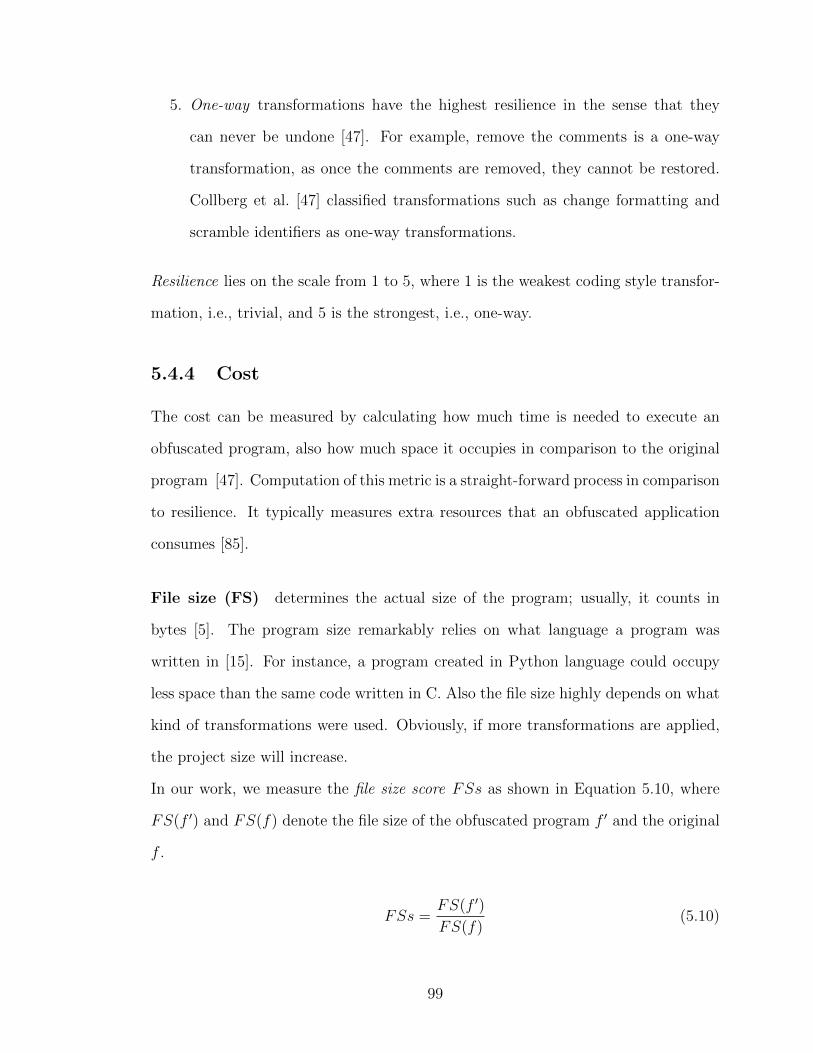
5. One-way transformations have the highest resilience in the sense that they
can never be undone [47]. For example, remove the comments is a one-way
transformation, as once the comments are removed, they cannot be restored.
Collberg et al. [47] classified transformations such as change formatting and
scramble identifiers as one-way transformations.
Resilience lies on the scale from 1 to 5, where 1 is the weakest coding style transfor-
mation, i.e., trivial, and 5 is the strongest, i.e., one-way.
5.4.4 Cost
The cost can be measured by calculating how much time is needed to execute an
obfuscated program, also how much space it occupies in comparison to the original
program [47]. Computation of this metric is a straight-forward process in comparison
to resilience. It typically measures extra resources that an obfuscated application
consumes [85].
File size (FS) determines the actual size of the program; usually, it counts in
bytes [5]. The program size remarkably relies on what language a program was
written in [15]. For instance, a program created in Python language could occupy
less space than the same code written in C. Also the file size highly depends on what
kind of transformations were used. Obviously, if more transformations are applied,
the project size will increase.
In our work, we measure the file size score FSs as shown in Equation 5.10, where
FS(f ′) and FS(f) denote the file size of the obfuscated program f ′ and the original
f .
FSs =FS(f ′)
FS(f)(5.10)
99

Execution time can be necessary if a program aims to perform a set of operations
quickly and efficiently.
In our work, we measure the execution time score ETs as shown in Equation 5.11,
where ET (f ′) and ET (f) denote the time, which was spent on running the obfus-
cated program f ′ and the original f .
ETs =ET (f ′)
ET (f)(5.11)
5.4.5 Detection
To evaluate the authors’ detection after coding style transformations, we use state-
of-the-art authorship attribution systems– Caliskan features (C ), Ding features (D),
Kothari features (K ), and our improved features (I).
We evaluate an author detection by calculating the average of the attribution accu-
racies (acc) of the aforementioned techniques after coding style transformations, as
shown in Equation 5.12.
Detection =acc(C) + acc(D) + acc(K) + acc(I)
4(5.12)
5.4.6 Results
Table 5.3 presents the evaluation of each transformation from Section 3.3 based on
metrics identified above, i.e., complexity (program length score, cyclomatic com-
plexity score, and nesting level score), readability, resilience, cost (file size score and
execution time score), and detection.
Program length score (PLs) This metric did not change with comment transfor-
mations, as such measurement depends on total number of operands and operators.
The transformation of curly brackets shows the same tendency, although with the
100

”One True Brace Style” coding style, program length increases 1.03 times. As shown
in Section 3.3, this transformation uses additional curly brackets to separate one line
conditional statements.
The program length of the rest of the layout (indentation, lines), all lexical and
part of syntactic (AST leave) transformations stay the same as before modification.
However, AST node transformation influences program length score: it decreases
0.93 times after changing ”for” to ”while” loop and increases to 1.02 after ”while”
to ”for”, since ”for” loop has additional initialization and increments statements in
comparison with ”while” loop. The transformations ”switch-case” to ”else-if” and
”else-if” to ”switch-case” shows the same tendency.
Program length score increases dramatically with control-flow and data-flow trans-
formations. Transformations of code logic show an increase to near 25 times. The
program length in predicates transformation increases from 25.19 to 31.19 which
depends on the type of predicates used. Even after merging and splitting transfor-
mations, the code increases in size as such transformations add additional formal
arguments to modify the signature of the function. In data-flow transformations,
the largest program size score is 52.98 and appears after transformation– string ob-
fuscation using string generation function.
Cyclomatic complexity score (CCs) This metric depends on the number of
predicates in a function; therefore it shows no change for all layout, lexical, and
syntactic transformations in Table 5.3, and they do not modify the program control
structures. However, we see an increase of 3 times with control-flow flattening. With
opaque predicates, the results show an increase from 2 to 4.75. For the rest of control-
flow transformations, the results show a decrease of 0.25 with function splitting and
a rise to 14 with function reordering with adding bogus arguments. For data-flow
transformations we see the increase in complexity from 1.2, 1.5, and 1.75, and the
highest score 21.75 with transformation– string obfuscation using string generation
101

function.
Nested complexity score (NLs) This metric measures the difference between
the nesting level of conditionals in original and obfuscated programs. Results show
that this metric did not change with the layout, lexical, and syntactic transforma-
tions. The complexity of the code after control-flow flattening transformation shows
an increase of more than 9 times that of the original program. After flattening the
control-flow, the CFG nodes, which were initially at different nesting levels, are all
on the same nesting level after modification. The opaque predicates transformations
increase from 9.34 to 9.64, which depends on the opaque used in the transformation;
opaque predicates with question gives higher nested complexity. Aggregation and or-
dering transformations do not change the nested complexity. The complexity score
of data-flow transformations ranges from 9.26 to 9.56 on average.
Readability This metric is generally much higher for layout, lexical, and syntactic
than control-flow and data-flow transformations, as this metric highly depends on
program volume and length of the code.
After comment transformations, the readability score changes from 0.99 to 0.87,
where the minimum score in this category is given by– deleting all comments. With
such a transformation, the length of the code is decreased, which influences the
readability score. In curly brackets, the transformations which produce the less
readable code are Pico and Lisp styles, as these styles use the minimum number of
lines in comparison with others.
For indentation, using only tab characters and removing all indentation gives the
minimum readability score– 0.76 and 0.78, respectively. In line transformations,
deleting all empty lines brings a significant decrease in readability score to 0.67. With
such transformation of the length of code decreased, which affects the readability
score.
102

Name transformations do not change the readability score too much, only to 0.91.
However, with AST bigram transformations– changing ”else-if” to ”switch-case”–
the readability score decreases to 0.87; with control-flattening transformations, read-
ability scores decrease dramatically to 0.59. We can see further decreases when
applying opaque predicates transformations. It ranges from 0.41 to 0.43, as such
transformations have high scores in program length. With the rest of control-flow
transformations– aggregation and ordering– it varies from 0.41 to 0.68. Data-flow
transformations show an even further decrease to 0.4 of readability score.
Resilience Almost all layout, lexical, and syntactic transformations are one-way,
as they cannot be undone, i.e., have resilience score 5. For example, after obfuscating
a bracket style, we cannot come back to the original form, as we do not know what
type was used previously. Also, with transformation– adding comments to code on
each line, we can remove all comments, although it is not clear what comments
the original author wrote, i.e., what comments should be left. The same situation
exists with transformation– adding empty lines after each non-empty line– as we can
remove these empty lines, but it is not clear what kind of empty lines were left blank
by the original author (i.e., how much and where).
Control-flow and data-flow transformations are less resilient to deobfuscation. Sim-
ple control-flow flattening transformations can be deobfuscated using purely static
techniques, as shown by Udupa et al. [135]. They implemented control-flow deob-
fuscations by deleting spurious edges of the control-flow graph, which were attached
after this transformation. To measure the effectiveness of their deobfuscation, they
computed control-flow edges before and after modification; they were able to elimi-
nate about 73% of edges introduced by basic control-flow flattening transformations.
The authors stated that their method could not work with more complex control-
flow flattening transformations. We identify such transformation with trivial to weak
resilience, i.e., with a score from 1 to 2.
103

Due to the high popularity of opaque predicates transformations, several attacks
were published in the literature. Dalla Preda et al. [53] proposed a method based
on abstract interpretation to attack number theoretic opaque predicates. However,
Rinsma et al. [116] provided an IDA Pro plugin called Drop which can detect and
remove opaque predicates. Their approach was not highly precise. Only 7 out of 9
opaque predicates were discovered correctly. We can say that opaque predicates still
can be identified as transformations with trivial to weak resilience (with a score from
1 to 2).
Rugaber et al. [118] introduced an attack on programs, which were used merging
functions obfuscation. Their attack works by discovering the location of code lines,
which were used originally in different methods, and placing them into separate
methods. Unfortunately, they did not provide any experimental support to prove
their theory. We identify such transformations as strong (with score 3).
Griffin et al. [76] presented a theoretical method, which was able to recover original
data from the obfuscated code, therefore fully break reordering variables transfor-
mation. This study was mostly theoretical (no experiments were done to prove if the
proposed attack works), therefore we identify this transformation as a strong (with
score 3).
The drawback of the approach of encoded arithmetic is that the deobfuscation of this
transformation only depends on the attacker’s time, because only a small number
of these transformations are currently known [138]. Eyrolles et al. [63] stated that
it is possible to identify a deobfuscation method for each of them. They identified
encoded arithmetic transformation as weak (with score 2).
Encoded literals transformation has been deobfuscated by semantic attacks presented
by Banescu et al. [31]. These attacks are based on symbolic execution. We identify
such transformations as weak (with score 2).
For encoded data transformations, Guinet et al. [77] proposed a software Arybo,
104

which is based on static and semantic analysis. It can recover the original data
by simplifying obfuscated expressions. Although their attack cannot be potentially
conducted, as the full implementation was not provided. We identify such transfor-
mations as strong (with score 3).
File size score (FSs) Layout transformations decrease the file size almost by half,
for example deleting all comments transformation. However, this metric can increase
by 2.46 times with a transformation such as adding pure comments on each line and
one inline comment. With curly brackets transformation, the size of the obfuscated
program is slightly changed from 0.97 (Pico style) to 1.13 (GNU style). Indentation
transformations have a file size score from 0.87 (with removing all spaces or tabs
padding) to 2.57 (with indenting using (from 2 to 20) number of spaces per indent).
For lines transformations, the file decreases to 0.93 with deleting all empty lines and
increases to 1.17 with adding empty lines after each nonempty line transformations.
For lexical transformations changing all names to short decreases the file size 0.59
times. However, if adjusted to long names, the size increases 1.96 times. For syntactic
transformations, the file score ranges from 0.91 to 1.24. With control-flow transfor-
mations, the file size increases dramatically almost five times, with a minimum– 4.27
of control-flow flattening– to 4.68 of opaque predicates. However, aggregation and
ordering almost do not change the file size. With data-flow transformations, the file
size increases even more to 6 times.
Execution time score (ETs) Because our dataset was generated by selecting
random source code from GitHub, there are programs which are not executed, be-
cause they have a lack of necessary dependencies or libraries which they rely on. Only
253 files from 750 were executed correctly. As a result, we measured the execution
time only of those files.
Layout, lexical, and syntactic transformations did not change this metric. Although
105
with control-flow transformations, which aims to transform logic and predicates,
the execution time increases from 4.27 to 4.68 times, depending on the type of
transformations. However, the rest of the control-flow transformations– aggregation
and ordering– increases time from 1.01 to 1.17. With data-flow transformation, it
ranges from 4.13 to 5.38.
Detection Initially, the average authorship attribution accuracy on GitHub C
dataset was 66.14%. This value was based on averaging the scores depicted in
Table 4.1: 44.13% with Ding features, 74.4% with Caliskan features, 62.3% with
Kothari features, and 83.73% with our improved features.
With layout transformations of comments, the accuracy ranges from 65.33% to
41.88%. With the lowest accuracy achieved when deleting all comments transfor-
mation is applied. For curly brackets transformations, the attribution performance
dropped from 66.14% to 51.48%, when using Pico brackets style; other transfor-
mations only slightly change the accuracy. With indentation transformations, the
lowest accuracy was achieved with removing all space and tabs padding and it equaled
43.34%. And with lines transformation the lowest accuracy was 49.23% by adding
empty lines after each non-empty line transformation. Such results can be explained
by looking on the nature of the selected feature groups– only Ding feature set com-
prised 28% of layout features, which can be easily obfuscated by our layout trans-
formations. The rest of Caliskan, Kothari and our improved feature sets have only
0.42%, 0%, and 1.14% layout features, respectively (shown in Table 4.1). As a result,
these sets are resistant to layout transformations. Overall, the average accuracy of
all feature sets did not change much.
With lexical and syntactic transformations, the possibility of detection decreased to
34.42% (by changing names to long names) and to 12.39% (by using unique names
for every author) since lexical features consist of 71.43%, 33.31%, 100%, and 41.18%
with Ding, Caliskan, Kothari, and our improved feature sets, respectively.
106

Control-flow and data-flow transformations dropped accuracy to 15.32% and 34.42%.
The maximum decrease was received control-flow flattening with computing dispatch
and replacing integer arithmetic transformations. Since such transformations in-
crease the initial program significantly by adding redundant code, which influences
not only control-flow and data-flow features, but also the layout, lexical, and syn-
tactic features.
Summary In this section, we evaluated each proposed coding style transformation
with respect to its complexity (How complex had the obfuscated program become?),
readability (How easy was it for a human to read the modified code?), resilience
(How difficult is it to construct a deobfuscated tool that can return the original
coding style?), cost (How much did time and space of the program change?), and
detection (How good are the current authorship attribution techniques in detecting
the author of obfuscated code?).
We found that almost every layout and lexical transformation was low-cost and there-
fore could be applied on any software with practically no computational overhead,
and most of them preserved readability. The main drawback of such transforma-
tions, when considered separately, was that they could not entirely hide the coding
style of the author; the detection range changed from 65.47% to 34.42% with each
transformation.
We noticed that the rest of syntactic, control-flow, and data-flow transformations
made the target program much slower, larger, and much harder to read than the
original. The advantage of such transformations, when used alone was that some of
them reduced detection to almost 12.39%.
Perhaps, the combination of these transformations, for example, comments (from
layout) and opaque predicates (from control-flow), could reduce further the detection
rate. We explore this hypothesis in the next section.
107

Coding style transformations Evaluation metricsLevel Target Transformation Complexity Readability Resilience Cost Detection
PLs CCs NLs FSs ETs
Layout
Comments
To Block comments 1 1 1 0.98 5 1 1 65.33%To Javadoc comments 1 1 1 0.99 5 1 1 64.91%To Line comments 1 1 1 0.99 5 0.99 1 64.26%To pure comment lines 1 1 1 0.98 5 0.99 1 65.17%Delete all inline comments 1 1 1 0.91 5 0.56 1 49.41%Delete all pure comment lines 1 1 1 0.90 5 0.69 1 43.86%Delete all comments 1 1 1 0.87 5 0.55 1 41.81%Add pure comments on each line 1 1 1 0.99 5 1.67 1 53.42%Add inline comments on each line 1 1 1 0.99 5 1.64 1 52.33%Add pure comments on each line and one inline comment 1 1 1 0.99 5 2.46 1 49.27%
Curly brackets
To Allman style 1 1 1 0.99 5 1 1 56.21%To Java style 1 1 1 0.99 5 0.98 1 63.23%To Kernigan and Ritche style 1 1 1 0.99 5 0.97 1 65.47%To Stroustup style 1 1 1 0.99 5 0.99 1 65.23%To Whitesmiths style 1 1 1 0.99 5 1.08 1 64.99%To VTK 1 1 1 0.98 5 0.99 1 53.45%To Banner style 1 1 1 0.97 5 1.02 1 65.23%To GNU style 1 1 1 0.97 5 1.06 1 61.23%To Linux style 1 1 1 0.96 5 1.13 1 64.77%To Horstmann style 1 1 1 0.96 5 0.98 1 53.45%To ”One True Brace Style” 1.03 1 1 0.96 5 0.99 1 59.87%To Google style 1 1 1 0.96 5 0.98 1 57.33%To Mozilla style 1 1 1 0.97 5 0.99 1 56.21%To Pico style 1 1 1 0.95 5 0.97 1 51.48%To Lisp style 1 1 1 0.95 5 0.98 1 61.23%
Indentation
Indent using (from 2 to 20) number of spaces per indent 1 1 1 0.96 5 2.57 1 61.23%Indent using tabs for indentation and spaces for line alignment 1 1 1 0.93 5 1.59 1 58.31%Indent using all tab characters, if possible 1 1 1 0.76 5 1.21 1 51.23%Indent using mix of tabs and spaces 1 1 1 0.97 5 1.83 1 54.5%Insert space padding around operators 1 1 1 0.99 5 1.08 1 52.3%Insert space padding after only commas 1 1 1 0.78 5 1.05 1 62.6%Insert space padding around parenthesis on both side 1 1 1 0.99 5 1.09 1 61.2%Insert space padding around parenthesis on the outside only 1 1 1 0.89 5 1.08 1 63.34%Insert space padding around parenthesis on the inside only 1 1 1 0.91 5 1.08 1 62.3%Insert space padding between ’if’, ’for’, ’while’ 1 1 1 0.99 5 1.1 1 61.3%Remove extra space padding around parenthesis 1 1 1 0.89 5 0.98 1 59.2%Remove all space or tabs padding 1 1 1 0.78 5 0.87 1 43.34%
Lines
Delete empty lines within a function or method 1 1 1 0.91 5 0.97 1 59.67%Delete all empty lines 1 1 1 0.67 5 0.93 1 52.83%Write each statement in one line 1 1 1 0.91 5 1.08 1 61.4%Write several statements in one line 1 1 1 0.87 5 0.99 1 53.23%Write one declaration per line 1 1 1 0.89 5 1.12 1 51.32%Write several declarations in one line 1 1 1 0.78 5 0.94 1 52.93%Add empty line after each nonempty line 1 1 1 0.99 5 1.17 1 49.23%
108

Coding style transformations Evaluation metricsLevel Target Transformation Complexity Readability Resilience Cost Detection
PLs CCs NLs FSs ETs
Lexical Names
Change all names on short name identifiers(one-two characters)
1 1 1 0.95 5 0.59 1 37.41%
Use dictionary to change names to long names (8-10 characters) 1 1 1 0.91 5 1.96 1 34.42%Change the first letter in identifiers to uppercase 1 1 1 0.99 5 1 1 53.24%Change the first letter to lowcase 1 1 1 0.99 5 1 1 59.5%The first sign is underscore/dollarsign 1 1 1 0.99 5 1.05 1 59.34%
Syntactic
AST leaves
Copy and insert all comments from imitated author 1 1 1 0.99 5 2.11 1 38.34%To imitate author B, change all name identifiers to the same namesused in author B code
1 1 1 0.99 5 1.12 1 23.42%
All names are unigue for everyauthor (use different dictionaries to change the names)
1 1 1 0.99 5 1.24 1 12.39%
Use the same dictionary to change names for every author 1 1 1 0.99 5 0.99 1 42.8%
AST nodes
Change ”for” to ”while” loops 0.93 1 1 0.99 5 1.07 1 59.23%Change ”while” to ”for” loops 1.02 1 1 0.99 5 0.91 1 57.93%Change ”else-if” to ”switch-case” 1.14 1 1 0.87 5 1.08 1 55.72%Change ”switch-case” to ”else-if” 0.95 1 1 0.99 5 0.93 1 52.8%
Control-flow
Logic
Control-flow flattening with ”switch” dispatch 25.17 3 9.39 0.61 1 ∼ 2 3.05 4.28 23.43%
Control-flow flattening with ”go-to” dispatch 25.11 3 9.39 0.59 1 ∼ 2 3.07 4.27 19.87%Control-flow flattening with normal branch 25.11 3 9.39 0.61 1 ∼ 2 3.05 4.27 19.87%Control-flow flattening with computing branch 25.28 3 9.34 0.53 1 ∼ 2 3.47 4.35 15.32%
Predicates
Opaque predicates with call to random existing function,when false 25.19 3.25 9.39 0.42 1 ∼ 2 3.39 4.57 24.3%Opaque predicates with call to non-existing function, when false 31.19 4.75 9.39 0.41 1 ∼ 2 3.35 4.59 25.4%Opaque predicates with call to existing statement, when true 31.18 2 9.56 0.43 1 ∼ 2 3.35 4.57 24.3%Opaque predicates with question 25.21 2.75 9.64 0.42 1 ∼ 2 3.37 4.68 21.2%
AggregationFunction merging 25.11 1 1 0.61 3 3.09 1.01 19.32%Function splitting 25.14 0.25 1 0.68 3 3.21 1.03 17.5%
OrderingFunction argument reoder 25.16 3 1 0.53 3 3.39 1 52.91%Function argument reoder with adding bogus arguments 25.13 14 1 0.41 3 3.45 1.17 49.34%
Data-flowLiterals
Integer obfuscation using opaque expressions 26.76 1.5 9.55 0.4 2 6.57 5.38 41.34%String obfuscation using string generation function 52.96 21.75 9.56 0.45 2 6.4 4.95 39.81%
Data Variable obfuscation using linear transformation 28.96 1.2 9.26 0.44 3 6.4 4.13 38.34%Arithmetic Arithmetic obfuscation using boolean expressions 25.14 1.75 9.34 0.41 2 6.42 4.28 34.42%
Table 5.3: Applied transformations and their evaluation
109

Ding et al.’s[55]
Caliskan et al.’s
[44]
Improved
Kothari et al.’s[91]0
102030405060708090
100
Features
Acc
ura
cy
Origin Beatify Code Convention PrettyPrinter
Figure 5.2: Percentage of correctly classified authors after using the following for-matting: Beatify, Code Convention and PrettyPrinter on original source code
5.5 Author obfuscation techniques evaluation
To evade author imitation attack, one could use code formatting to produce a more
generic less personal version of the code. Alsulami at al. [28] stated that current
IDEs often modify programs using different formatting practices and coding style
conventions. Such formatting reduces the confidence of identification of the authors
of source code. Indeed, many software development standards dictate a formatting
style that developers have to adhere to. We hypothesize that the use of a particular
style alone is not sufficient to avoid attribution. Figure 5.2 shows our preliminary
experiments with several different types of formatting: Beautify, Java Code Conven-
tion, PrettyPrinter using the Eclipse Code Formatter. It indicates that attribution
accuracy does not produce significant change after using such formatting tools. We
could still attribute nearly half of the authors with the Ding feature set and more
than 70% of the authors with other feature sets. After manual analysis of our data,
we found that near 80% authors in our datasets were already following Java Code
Convention.
110

origi
nlib
s
allman
banner
horstm
ann
java kr
linux lis
ppico
strou
strup
vtk
102030405060708090
100
Brackets transformations
Acc
ura
cy
Figure 5.3: Percentage of correctly classified authors after brackets transformationfor GoogleCodeJam Java dataset
Our goal is to offer an author obfuscation technique that preserves the readability
of the code and misleads existing authorship attribution tools. We have seen that
the current methods for authorship attribution leverage layout and lexical features
(Ding and Kothari feature sets) or layout, lexical, and syntactic (Caliskan and our
improved feature sets).
In addition to these features, we also look at transforming the control-flow and data-
flow of a program. Although specific transformation can vary depending on the goal
of the analysis, in this study, we experimented with the transformations specified in
Table 5.3.
For example, in the group brackets, we explore all possible styles of curly brackets
(parentheses) that a developer can use. Figure 5.3 shows the results of experiments
with the only transformation of brackets in the code. We use 11 different styles of
brackets. By changing the bracket style to Pico (the most rarely used by devel-
opers), we can reduce the attribution rate for the Ding feature set from 73.84% to
11.29%. The worst result is obtained with Java style (66.84%), this implies that
most authors in our dataset use Java style. When considering the Caliskan feature
set, the accuracy results do not change much and are still around 97%. Since the
111

layout features make up only 1% of the Caliskan feature set after information gain
feature selection. We observe the same tendency with the Kothari and our improved
features. The average detection rate of four feature sets is still high. To decrease the
attribution accuracy more, we propose the following obfuscation methods, which are
created by using different combinations of coding style transformations.
We define ”HideByCosine” obfuscation as following:
Definition 5.5.1 (“HideByCosine” obfuscation). Let P → P ′ be a transformation
of a source program P into a target program P ′. In order for P → P ′ to be a
“HideByCosine” obfuscation the following steps should be applied:
• Apply a set of transformations Tn from the list of possible transformations T
on program P
• Select those transformations Ti so that CosSim(~a,~b) → min, where ~a is the
feature vector of the original program and~b is the feature vector of the modified
program.
The setup of our experiment for ”HideByCosine” is similar to that of an imitation
attack (from Section 5.3); we train the classifier on the non-obfuscated code and
test it on the obfuscated one. Such setup is reflected in our defined adversarial
model with adversary’s capability of manipulating testing data and adversary’s goal
of untargeted misclassification (from Section 5.2).
The results of the evaluation process for ”HideByCosine” method are reported in
Table 5.5. When using the only layout, lexical, and syntactic transformations we
can achieve 1.08% attribution rate after applying ”HideByCosine” obfuscation for
the Ding feature set. The transformations are unique for each author. With the
Caliskan feature set we drop accuracy from 97.31% to 39.43% for the GoogleCodeJam
Java dataset, 80.92% to 27.96% for the GitHub Java dataset, and 74.4% to 21.27%
for the GitHub C dataset. Since Caliskan et al. [44] uses information gain to select
112

Lexical SyntacticFeatures Layout
unigrams non-unigrams leaves non-leavesAll
GCJ JavaOriginal 6 20544 20 17393 667 38630
After information gain 6 187 0 342 72 607GitHub Java
Original 6 87229 20 136415 808 224478After information gain 5 197 6 405 74 687
GitHub COriginal 6 403972 20 569128 29063 1002189
After information gain 6 395 9 899 123 1432
Table 5.4: Effect of information gain feature selection using Caliskan et al. [44]approach
the most informative features, most of the remained features are term frequency of
unigrams and leaves (near 87% for GoogleCodeJam, GitHub Java and C datasets),
which can be easily modified by name transformations. Table 5.4 shows the statistics
of Caliskan features after information gain feature selection. The next group is AST
nodes and AST node bigrams features (two AST nodes that are connected [44]),
which only represent 12%, and are part of syntactic features. A portion of them can
be obfuscated with simple transformations, e.g., changing ”for” to ”while” loops,
and ”else-if” to ”switch-case”, therefore do not guarantee author style’s hiding. As a
result, we applied control-flow and data-flow transformations on the top. After such
transformations 0% of authors can be successfully attributed by Caliskan and Ding
features.
Note that our result differs from that reported in the Caliskan et al.’s [44] work. The
authors claimed that their method is resistant to simple transformations, such as
provided by Stunnix with the reported accuracy of 98.89%, and to more sophisticated
transformations (e.g., function virtualization by Tigress obfuscator) with 67.22% on
GoogleCodeJam data. Our results showed significantly lower accuracy due to two
facts. First, the authors used a much smaller dataset with only 20 authors making
the task of attribution easier. Second, the experimental setup offered by their study
assumed that the adversary is manipulating the training data and thus training of
the classifiers is performed on selected and already obfuscated features.
113

We, however, followed a more realistic scenario commonly used in adversarial ma-
chine learning, i.e., the adversary aims to evade detection by manipulating test sam-
ples only [36]. We thus trained the RandomForest classifier on non-obfuscated code
and tested it on obfuscated samples (imitated code samples in the case of imitation
attack). We were able to hide the coding style of the author with lexical and syntactic
features and decrease the attribution accuracy dramatically to 39.43% for GoogCode-
Jam Java, to 27.96% for GitHub Java, and to 21.27% for GitHub C datasets. After
adding control-flow and data-flow transformations, no authors were recognized.
Generalization of author obfuscation method for any author style The
proposed author obfuscation method ”HideByCosine” requires that every time au-
thors want to hide their identity they should first identify the code transformations
that generate the most distinctive style concerning their style. The goal now is to
define transformations which are unique across all authors. We are doing this by
considering one transformation from each group given in Table 5.3. We transform
the source code of all authors by using these transformations and then perform clas-
sification again. In this way, for example, we can identify the bracket styles that
are used the least in a considered dataset and then modify each author’s brackets
style by using this type of brackets. It gives us the opportunity to find a unique
anonymous style that hides the coding style of all the authors in the dataset. We
refer to these author obfuscation methods as “MaxiCode” and ”MiniCode”. The
methodology of finding such transformations presents in Algorithm 5.1.
After applying Algorithm 5.1 to our datasets, we found set of transformations Tk,
which were unique across all authors in our dataset. The proposed author obfuscation
method based on these transformations is described in Definition 5.5.2.
Definition 5.5.2 (“MaxiCode” obfuscation). Let P → P ′ be a transformation of a
source program P into a target program P ′. For P → P ′ to be a “MaxiCode” ob-
114

Algorithm 5.1 Author obfuscation ”MaxiCode” or ”MiniCode”
Input: Dataset Vs with number of authors s and number of source code samples mfor each author; List of possible transformations T
Output: Set of transformations Tk from T
for all Vs doapply each transformation Ti from T
if after transformation Ti attribution fails to attribute code samples m toauthors s then
return Tiend if
end forreturn Tk = {Ti}li=1, where l- number of transformations in set Tk
fuscation the following transformations Tk should be applied to the original program
P :
• Layout (T1 : add pure line comments on each line, T2 : use pico style for
brackets, T3 : indent using tabs for indentation, T4 : add empty line after each
non-empty line);
• Lexical (T5 : the first sign is underscored with long names);
• Syntactic (T6 : all names are unique for every author; T7 : change ”while” to
”for”, T8 : change ”else-if” to ”switch-case”);
• Control-flow (T9 : control-flow flattening with normal branch; T10 : function
splitting;
• Data-flow (T11 : integer obfuscation using opaque expression)
One of the obvious concerns with this method is the size of the source code since
these transformations almost triple the code size. Such an increase makes these
transformations impractical to use for developers in open-source projects. A possible
solution is to shrink the code instead of expanding it; we refer to this method as
“Minicode”.
115

Definition 5.5.3 (“MiniCode” obfuscation). Let P → P ′ be a transformation of a
source program P into a target program P ′. In order for P → P ′ to be a “MiniCode”
obfuscation the following transformations Tk′ should be applied to original program
P :
• Layout (T1 : no comments, T2 : use pico style for brackets, T3 : remove all space
or tabs padding, T4 : delete all empty lines );
• Lexical (T5 : the first sign is underscored with short names);
• Syntactic (T6 : all names are unique for every author; T7 : change ”for” to
”while”, T8 : change ”switch-case” to ”else-if”);
• Control-flow (T9 : control-flow flattening with normal branch; T10 : function
merging);
• Data-flow (T11 : string obfuscation using string generation function)
The difference between “HideByCosine” method and “MaxiCode” (“MiniCode”)
method that we proposed is that the former one is more about modifying the indi-
vidual author’s style to the most dissimilar one; thus for every author the method
identifies different transformations, while the latter method is about finding a unique
style that protects the style of all authors. The main advantage of using the obfusca-
tion “MiniCode” or “MaxiCode” for author obfuscation is that authors do not need
to make any precomputations beforehand.
Table 5.5 shows how the accuracy of attribution changes after applying the “Mini-
Code” approach to each feature set. This method decreases the size of the program
by almost 8 times, while still preserving readability. After MiniCode obfuscation,
the Kothari feature set achieves 1.88% attribution accuracy (GoogleCodeJam Java
dataset), 0% accuracy (GitHub Java), and 4.56% accuracy (GitHub C). As the
116

Author obfuscationEvaluation metrics
Complexity Read Resil Cost DetectionPLs CCs NLs FSs ETs D C K I Aver
GoogleCodeJam Java dataset
Layout level
HideByCosine 1 1 1 0.89 5 1.09 1 7.12% 92.32% 80.32% 83.23% 65.75%
MaxiCode 1 1 1 0.92 5 1.75 1 9.83% 95.65% 83.45% 85.65% 68.65%
MiniCode 1 1 1 0.74 5 0.58 1 10.43% 96.4% 83.96% 86.73% 69.38%
Layout+Lexical levels
HideByCosine 1 1 1 0.86 5 1.32 1 4.23%% 48.4% 15.32% 41.25% 27.3%
MaxiCode 1 1 1 0.91 5 1.98 1 6.11% 50.78% 18.56% 46.48% 30.48%
MiniCode 1 1 1 0.72 5 0.68 1 6.43% 52.78% 19.92% 48.23% 31.84%
Layout+Lexical+Syntactic levels
HideByCosine 1.01 1 1 0.84 5 1.54 1 1.08% 39.43% 1% 32.43% 18.49%
MaxiCode 1.08 1 1 0.89 5 2.32 1 4.12% 41.04% 1.97% 35.38% 20.63%
MiniCode 0.81 1 1 0.69 5 0.87 1 4.28% 43.90% 1.88% 37.88% 21.99%
Layout+Lexical+Syntactic+Control-flow levels
HideByCosine 7.48 3.21 4.26 0.63 5 3.21 2.31 0% 0% 0% 0% 0%
MaxiCode 8.12 3.11 4.98 0.68 5 5.78 2.11 0% 0% 0% 0% 0%
MiniCode 6.23 2.98 4.14 0.51 5 1.98 1.78 0% 0% 0% 0% 0%
GitHub Java dataset
Layout level
HideByCosine 1 1 1 0.86 5 1.23 1 5.42% 75.91% 76.32% 72.91% 57.64%
MaxiCode 1 1 1 0.9 5 1.87 1 7.31% 78.23% 78.91% 74.81% 59.82%
MiniCode 1 1 1 0.71 5 0.59 1 7.98% 79.11% 80.23% 75.69% 60.75%
Layout+Lexical levels
HideByCosine 1 1 1 0.84 5 1.43 1 2.21% 31.28% 10.21% 30.29% 18.49%
MaxiCode 1 1 1 0.89 5 2.12 1 3.11% 33.42% 13.76% 35.94% 21.56%
MiniCode 1 1 1 0.65 5 0.71 1 3.81% 34.51% 14.23% 37.15% 22.43%
Layout+Lexical+Syntactic levels
HideByCosine 1.02 1 1 0.82 5 1.69 1 0% 27.96% 0% 12.38% 10.01%
MaxiCode 1.11 1 1 0.85 5 2.92 1 2.37% 28.67% 0% 15.64% 11.67%
MiniCode 0.89 1 1 0.62 5 0.89 1 2.49% 30.29% 0% 16.43% 12.3%
Layout+Lexical+Syntactic+Control-flow levels
HideByCosine 13.92 3.98 5.37 0.56 5 3.98 3.56 0% 0% 0% 0% 0%
MaxiCode 14.51 3.76 5.98 0.6 5 6.23 3.21 0% 0% 0% 0% 0%
MiniCode 12.93 3.15 4.39 0.49 5 2.12 2.98 0% 0% 0% 0% 0%
GitHub C dataset
Layout level
HideByCosine 1.01 1 1 0.83 5 1.13 1 3.21% 69.47% 68.11% 65.12% 51.48%
MaxiCode 1 1 1 0.87 5 1.96 1 4.68% 72.89% 70.23% 67.34% 53.79%
MiniCode 1 1 1 0.67 5 0.61 1 4.92% 73.87% 71.15% 67.91% 54.46%
Layout+Lexical levels
HideByCosine 1.01 1 1 0.81 5 1.56 1 1.47% 25.83% 8.96% 23.11% 14.84%
MaxiCode 1 1 1 0.86 5 2.54 1 1.99% 27.76% 8.13% 24.97% 15.71%
MiniCode 1 1 1 0.61 5 0.79 1 2.31% 28.11% 7.21% 25.11% 15.68%
Layout+Lexical+Syntactic levels
HideByCosine 1.02 1 1 0.79 5 1.87 1 0% 21.27% 3.56% 5.92% 7.69%
MaxiCode 1.15 1 1 0.83 5 3.56 1 1.23% 22.99% 4.11% 7.12% 8.86%
MiniCode 0.91 1 1 0.59 5 0.91 1 1.56% 23.76% 4.56% 7.96% 9.46%
Layout+Lexical+Syntactic+Control-flow levels
HideByCosine 35.24 5.75 9.49 0.53 5 4.29 4.98 0% 6.87% 0.23% 3.76% 2.72%
MaxiCode 36.26 5 9.59 0.56 5 7.92 4.58 0.46% 9.69% 1.79% 5.12% 4.27%
MiniCode 33.14 4.25 9.11 0.41 5 2.72 4.31 0.73% 9.92% 1.88% 5.98% 4.63%
Layout+Lexical+Syntactic+Control-flow+Data-flow levels
HideByCosine 62.99 16.45 12.54 0.39 5 10.98 9.34 0% 0% 0% 0% 0%
MaxiCode 79.45 26.75 14.76 0.43 5 15.78 9.59 0% 0% 0% 0% 0%
MiniCode 61.23 5.89 14.12 0.25 5 8.87 9.27 0% 0% 0% 0% 0%
Table 5.5: Results of author obfuscation methods on all datasets117

Kothari feature set is composed of layout and lexical features, these features can
be obfuscated by our transformations.
With the third dataset, i.e., Github C dataset, only to make the layout, lexical, syn-
tactic, and control-flow transformations seems not enough, as there are still authors
who were attributed correctly, the detection decreased to 6.87% with HideByCo-
sine, 9.69% with MaxiCode and 49.92% with MiniCode of the Caliskan feature set.
The first reason is that long code contains more personal style features, than small
code, which makes the author obfuscation much harder. The second reason is that
our Github C dataset contains more authors and more samples per author than
Github Java dataset or GoogleCodeJam Java dataset, which can reflect the differ-
ence of author obfuscation performance. After applying data-flow transformations
the detection decreases to 0% with all attribution features– Ding (D), Caliskan (C),
Kothari (K), and our improved (I) sets.
5.6 Threats to validity
The results of this research have some potential limitations. In this section, we
discuss the conclusion, internal, construct, and external validity of our study.
Threats to conclusion validity These threats are mostly concerned about whether
there is a relationship between the cause and effect 1.
One of the threats to the conclusion validity of this study is the use of the Weka
tool with the right settings, which affect the learning process. Thus, the parameters
considered in our experiments may influence attribution accuracy. To mitigate this
threat, we set all Weka parameters according to the settings defined in Caliskan et
al. [44] and Burrows et al. [42] studies. To avoid the problem with over-fitting, we
used k-fold cross-validation, where k is the number of samples in the dataset.
1http://www.socialresearchmethods.net/kb/concval.php
118

Threats to internal validity These threats are mostly concerned about whether
the observed correlation reflect a causal dependence between the cause and effect 2.
1. The first threat to internal validity is associated with our replication and data
analysis. To ensure the internal validity of our replication study, we requested
the original datasets employed by previous studies in code authorship attri-
bution. Out of the 27 datasets from the 21 reviewed studies, we were able to
collect 7 datasets (as discussed in Chapter 4). Thus, our replication and data
analysis were performed by using these 7 datasets. Those datasets, however,
provide a sufficient representation of experimental data type used in the field.
As for the used features in the replication and data analysis, we analysed
features from each of the 21 reviewed studies. We found that some of the
works reused the features of their predecessors (for example, Simko et al. [125]
and Dauber et al. [54] used features from Caliskan et al. [44] study) or some
feature sets were created by improving previous studies (for example, Ding et
al. [55] employed features from MacDonell et al. [96] study for Java language,
in turn, MacDonell et al. [96] improved features from Krsul et al. [92] study by
measuring features significance). Thus, for our replication and data analysis,
we selected three feature sets that were the most prominent in the history of
source code attribution and are often seen as benchmark features.
2. Another threat to internal validity corresponds to the changes in the dataset (or
features) to the results of our author imitation and author obfuscation exper-
iments. To mitigate this threat, we conducted experiments on three different
datasets with different data sizes, sources, and languages. These datasets were
extracted randomly and automatically, therefore it represents typical data for
those sources. To evaluate our author imitation and obfuscation, we used fea-
ture sets from three existing benchmark studies and our improved features.
2http://www.socialresearchmethods.net/kb/intval.php
119

The detection rate was calculated by averaging results of all four feature sets.
We also executed the experiments more than once to make sure that there are
no errors while performing the tests and that our results can be replicated.
Threats to construct validity These threats are mostly concerned about whether
our results can be generalized to the constructs 3.
One of the threats to the construct validity of this study is the use of accuracy as an
evaluation metric, instead of F-1 score, precision, or recall 4. Choosing an evaluation
measurement often depends on the type of problem being solved. In code authorship
attribution, the most commonly used evaluation metric is accuracy, which measures
the number of correct attributions from all predictions made. Thus, this metric was
used for evaluation in our study.
Threats to external validity These threats are mostly concerned about whether
our results are applicable or can be generalized to other data, features, and classifi-
cation algorithms 5.
1. Impact of dataset. Intuitively, we expect it to be more challenging to obfuscate
authors in the dataset with larger code samples, as they contain more personal
style features. Based on our experiments from Chapter 4, we showed that an
increasing number of lines in code makes the attribution task much easier, but
the author obfuscation more challenging. Also, we expect that increasing the
number of samples per author in the dataset will have the same influence on our
author obfuscation technique; therefore more transformations from different
levels will have to be applied to achieve 0% detection.
2. Impact of features. This work was concentrated in hiding features of the cod-
3http://www.socialresearchmethods.net/kb/constval.php4https://en.wikipedia.org/wiki/Precision and recall5http://www.socialresearchmethods.net/kb/external.php
120

ing style, which were most commonly used in source code attribution, such
as layout and lexical numerical features, syntactic, and n-grams. We expect
that it will be more challenging to obfuscate features, which represent only
control-flow and data-flow levels, i.e., those features, used by binary code at-
tribution [26] techniques. It can be explained by looking at our author ob-
fuscation transformations. Most of these transformations, 57 from 73, were
created for obfuscating layout, lexical, and syntactic levels, and only 16 from
73 were used for transforming control-flow and data-flow levels of the code. We
believe that our author obfuscation can still be used for deceiving binary code
attribution, although some of the binary-code features will be able to detect
the coding style of some authors correctly.
3. Impact of classification. For our classification, we used four common machine
learning classifiers: Random Forest, Naive Bayes, decision tree (J48) and k-
nearest neighbor (IBk). In Chapter 5, it was shown that Random Forest classi-
fier outperforms the other three. Thus, our experiments in the rest of our study
were done using a Random Forest classifier. Can our results be generalized to
other classifiers? Intuitively, we expect that machine learning algorithms, such
as decision tree and k-nearest neighbor, will give us the same results. We think
that our author obfuscation may be more challenging with deep learning algo-
rithms, for example, recurrent neural networks (RNNs) and convolutional deep
neural networks (CNNs). The reason is that the model complexity of RNNs
and CNNs classifiers allow neural networks to solve more complex classification
tasks, find unique patterns between features, which current machine learning
algorithms are not be able to find.
121

5.7 Summary
In this chapter, we explored the accuracy of attribution using currently existing au-
thorship attribution techniques in the presence of deception. We investigated the
feasibility of author imitation attack on open-source software repositories. Also, we
proposed several author obfuscation methods: ”HideByCosine”, ”MaxiCode”, and
”MiniCode”. The first method, ”HideByCosine”, worked individually with each au-
thor by obfuscating source code to a style that was the most different from that of
the user. This method had better performance compared to the other two. The other
two methods worked by finding one style which was unique for all authors. ”Maxi-
Code” modified the source code by extending it, which tripled its size. Conversely,
”Minicode” significantly reduced the size of the code. Also, we applied control-flow
and data-flow transformations to be able to entirely hide the coding style of the
author, which gave 0% attribution at the end. With both author imitation and
author obfuscation methods we could significantly decrease the accuracy of current
authorship attribution techniques. We also discussed the possible threats to validity
of our study.
122

Chapter 6
Conclusion and Future work
Existing authorship attribution research assumes that authors do not attempt to
disguise their coding style. In this thesis, we challenged this underlying assumption
and explored existing authorship attribution methodologies in the adversarial setting.
To understand what influences attribution accuracy, we presented the first (to the
best of our knowledge) systematic study of the effects of the choice of datasets in
code authorship attribution. In particular, we analysed the impact that the quality
of data (existence of common code) and the size of data (authors, samples, and code
size) had on the overall accuracy and feature selection. After analysing 21 state-of-
the-art studies and replicating their experiments, we made the following conclusions:
1. The reduction of common code in the datasets consequently resulted in a sig-
nificant decrease in attribution performance.
2. Increasing the number of authors brought a deterioration in performance.
3. The accuracy of attribution decreased with limited availability of samples per
author.
4. Short code with less than 50 lines was the most challenging for the attribution
task.
123

5. Performance of token and byte n-gram features was highly depended on the
code size.
6. The efficiency of Caliskan feature set could be further increased by more than
10% by removing correlated features and considering best-performing features
for every code size. The optimal feature sets of each line of code were defined
and offered to the research community.
As a result of our research, we created new datasets with no common code and
offered it to the research community in the hope of diversifying and strengthening
experiments in this field.
To assess current attribution systems, we defined an adversarial model based on
an adversary’s goals, knowledge, and capabilities. We presented an author imita-
tion attack on current authorship attribution techniques. Author imitation attack
identified a developer (the victim) and transformed the attacker’s source code to a
version that mimicked the victim’s coding style while retaining the functionality of
the original code. The attack success was measured by its ability to deter existing
attribution techniques from recognizing this code as an attacker’s code and by its
ability to imitate the victim author’s style.
Within this context, we investigated three existing source code attribution techniques
introduced by Ding et al. [55], Caliskan et al. [44], and Kothari et al. [91]. We
explored their accuracy and their potential to be deceived by author imitation attack.
Through our experiments, we showed that all these techniques were susceptible to
author imitation. We were able to successfully imitate 75.63% of the authors on
GoogleCodeJam Java dataset, 69.65% of the authors on GitHub Java dataset, and
68.52% of the authors on GitHub C dataset on average.
Finally, to subvert author imitation attack, we proposed several author obfuscation
techniques- HideByCosine, MaxiCode, and MiniCode. These techniques allowed us
to hide the coding style of the author entirely. Unlike existing obfuscation tools, this
124

novel obfuscation techniques used transformations that preserved code readability.
We evaluated each introduced coding style transformations and author obfuscation
techniques with respect to our proposed metrics– complexity, readability, resilience,
cost, and detection.
Our experiments showed the effectiveness of author obfuscation. Indeed, we were
able to reduce the accuracy of the Ding et al. [55] attribution system from 73.84%
of correctly classified authors to 1.08% by using only layout, lexical, and syntactic
transformations on the GoogleCodeJam Java dataset. We were also able to decrease
the accuracy of the Caliskan et al. [44] attribution system from 80.92% to 27.96%
on the GitHub Java dataset. The attribution accuracy of Kothari et al. [91] system
was decreased to 3.56% on the GitHub C dataset. By adding control-flow and data-
flow obfuscation transformations we were able further reduced the performance of
Caliskan et al. [44], Ding et al. [55], and Kothari et al. [91] systems to 0%. Our
results demonstrated that the identity of open-source software developers could be
fully hidden with our author obfuscation techniques.
Opportunities for future work. We proposed some future directions for the
research in code authorship attribution, as well as a number of improvements, can
be made to our author imitation attack and author obfuscation methods.
Starting with coding style transformations, the first opportunity to extend this work
is to create such changes of coding style, which can hide the author style entirely,
but require much lower cost, complexity with higher readability and resilience scores
then we proposed. In this work, we considered 73 transformations of layout, lexical,
syntactic, control-flow, and data-flow levels. We found that none of the considered
transformations alone can fully hide the code. Accordingly, we experimented with
their combinations, which showed that the detection rate could be decreased to 0%.
Possibly a very different approach could be taken to hide the coding style of the
author, using some form of code generation–take source code as input and generate
125

a new, valid source code that has the same functionality as the input source code
and causes misclassification.
The second opportunity is to develop more attacks by combining different objec-
tives of the attackers and their capabilities. In this work, we considered the goal of
the attacker of targeted misclassification (author imitation) with capability of ma-
nipulating testing data. Future work can be expanded by considering what type
of information about attribution system the attacker has available and how many
resources can be used by the attacker to perform this attack.
The third opportunity is to consider how specific data type (gaming, database, li-
brary, etc.) can influence the attribution and obfuscation performance. In this work,
we experimented with different data sizes, sources, and languages. We found that
such parameters have a direct influence on the results. Future work can be done in
evaluating, what effect on the accuracy it has, for example, selecting only gaming or
only database code.
Finally, in future work, more effort can be invested in finding source code features
which can be resistant to the proposed coding style transformations and author
obfuscation techniques. Furthermore, our research showed that the performance of
current attribution techniques could be significantly decreased: after removing the
common code in the datasets, when the author’s data is limited– only short code
samples or a few samples per author– after increasing number of authors in the
dataset. For advancing authorship attribution area, it is beneficial to create such
an attribution technique which will show a high accuracy independently to data
characteristics and data sources. Creating such a model could be based on our
results of the effect of data and feature characteristics on attribution performance,
as well as considering our large-scale reference dataset for evaluation, as our results
showed that such dataset is the most challenging for attribution task.
126

References
[1] Allman. https://en.wikipedia.org/wiki/Eric_Allman/, accessed May 9,2018.
[2] Allman style. https://en.wikipedia.org/wiki/Indentation_style#
Allman_style/, accessed May 9, 2018.
[3] Common lisp style guide. https://lisp-lang.org/style-guide/, accessedMay 9, 2018.
[4] Cyclomatic complexity. https://en.wikipedia.org/wiki/Cyclomatic_
complexity/, accessed May 9, 2018.
[5] Global standards for the microelectronics industry jesd100b01. https://www.jedec.org/standards-documents/, accessed May 9, 2018.
[6] Gnu coding standards. https://www.gnu.org/prep/standards/, accessedMay 9, 2018.
[7] Google java style guide. https://google.github.io/styleguide/
javaguide.html, accessed May 9, 2018.
[8] Horstmann style. https://en.wikipedia.org/wiki/Indentation_style#
Horstmann_style/, accessed May 9, 2018.
[9] Indentation style. https://en.wikipedia.org/wiki/Indentation_style.
html/, accessed May 9, 2018.
[10] Kernighan and ritchie style. https://en.wikipedia.org/wiki/
Indentation_style#K&R_style/, accessed May 9, 2018.
[11] Linux kernel coding style. https://www.kernel.org/doc/html/v4.10/
process/coding-style.html, accessed May 9, 2018.
[12] Linux style. https://en.wikipedia.org/wiki/Indentation_style#
Variant:_Linux_kernel/, accessed May 9, 2018.
[13] Mozilla style guide. https://developer.mozilla.org/, accessed May 9,2018.
127

[14] Oracle, java code convention. https://www.oracle.com/technetwork/java/javase/documentation/codeconventions-142311.html/, accessed May 9,2018.
[15] Software metrics and measurement. https://en.wikiversity.org/wiki/
Software_metrics_and_measurement/, accessed May 9, 2018.
[16] Stroustrup style. https://en.wikipedia.org/wiki/Indentation_style#
Variant:_Stroustrup/, accessed May 9, 2018.
[17] A system for detecting software similarity. https://theory.stanford.edu/
~aiken/moss/, accessed May 9, 2018.
[18] Tabs, spaces, and size of indentations. https://en.wikipedia.org/
wiki/Indentation_style#Tabs,_spaces,_and_size_of_indentations/,accessed May 9, 2018.
[19] Tigress. https://tigress.cs.arizona.edu/, accessed May 9, 2018.
[20] Tree. https://en.wikipedia.org/wiki/Tree_(data_structure), accessedMay 9, 2018.
[21] Using the right comment in java. http://www.javadude.com/posts/
20000304-comments/, accessed May 9, 2018.
[22] Vtk coding style guide. https://itk.org/Wiki/ITK/Coding_Style_Guide,accessed May 9, 2018.
[23] Whitesmiths style. https://en.wikipedia.org/wiki/Indentation_style#
Whitesmiths_style/, accessed May 9, 2018.
[24] Wordpress coding standards. https://codex.wordpress.org/WordPress_
Coding_Standards#Indentation/, accessed May 9, 2018.
[25] Frances E Allen. Control flow analysis. In ACM Sigplan Notices, volume 5,pages 1–19. ACM, 1970.
[26] Saed Alrabaee, Noman Saleem, Stere Preda, Lingyu Wang, and Mourad Deb-babi. Oba2: An onion approach to binary code authorship attribution. DigitalInvestigation, 11:S94–S103, 2014.
[27] Saed Alrabaee, Paria Shirani, Mourad Debbabi, and Lingyu Wang. On thefeasibility of malware authorship attribution. In International Symposium onFoundations and Practice of Security, pages 256–272. Springer, 2016.
[28] Bander Alsulami, Edwin Dauber, Richard Harang, Spiros Mancoridis, andRachel Greenstadt. Source code authorship attribution using long short-termmemory based networks. In European Symposium on Research in ComputerSecurity, pages 65–82. Springer, 2017.
128

[29] Harald Baayen, Hans Van Halteren, and Fiona Tweedie. Outside the caveof shadows: Using syntactic annotation to enhance authorship attribution.Literary and Linguistic Computing, pages 121–132, 1996.
[30] Upul Bandara and Gamini Wijayarathna. Source code author identificationwith unsupervised feature learning. Pattern Recognition Letters, 34(3):330–334, 2013.
[31] Sebastian Banescu, Christian Collberg, Vijay Ganesh, Zack Newsham, andAlexander Pretschner. Code obfuscation against symbolic execution attacks. InProceedings of the 32nd Annual Conference on Computer Security Applications,pages 189–200. ACM, 2016.
[32] Sebastian Banescu and Alexander Pretschner. A tutorial on software obfusca-tion. In Advances in Computers, volume 108, pages 283–353. Elsevier, 2018.
[33] Chandan Kumar Behera and D Lalitha Bhaskari. Different obfuscation tech-niques for code protection. Procedia Computer Science, 70:757–763, 2015.
[34] Robert Bendel and Abdelmonem Afifi. Comparison of stopping rules in for-ward stepwise regression. Journal of the American Statistical association,72(357):46–53, 1977.
[35] Vinod Polpaya Bhattathiripad. Judiciary-friendly forensics of software copy-right infringement. IGI Global, 2014.
[36] Battista Biggio, Igino Corona, Davide Maiorca, Blaine Nelson, Nedim Srndic,Pavel Laskov, Giorgio Giacinto, and Fabio Roli. Evasion attacks against ma-chine learning at test time. In Joint European conference on machine learningand knowledge discovery in databases, pages 387–402. Springer, 2013.
[37] Barry Boehm and Victor Basili. Software defect reduction top 10 list.Foundations of empirical software engineering: the legacy of Victor Basili,426(37):426–431, 2005.
[38] Robert Bohrer. Halstead’s criteria and statistical algorithms. In Proc. EighthAnn. Computer Science Statistics Symp., Los Angeles, pages 262–266, 1975.
[39] Steven Burrows. Source code authorship attribution. PhD thesis, RMIT Uni-versity, 2010.
[40] Steven Burrows and Seyed MM Tahaghoghi. Source code authorship attri-bution using n-grams. In Proceedings of the Twelth Australasian DocumentComputing Symposium, Melbourne, Australia, RMIT University, pages 32–39.Citeseer, 2007.
[41] Steven Burrows, Alexandra Uitdenbogerd, and Andrew Turpin. Application ofinformation retrieval techniques for source code authorship attribution. In In-ternational Conference on Database Systems for Advanced Applications, pages699–713. Springer, 2009.
129

[42] Steven Burrows, Alexandra Uitdenbogerd, and Andrew Turpin. Comparingtechniques for authorship attribution of source code. Software: Practice andExperience, 44(1):1–32, 2014.
[43] Raymond Buse and Westley Weimer. A metric for software readability. In Pro-ceedings of the 2008 international symposium on Software testing and analysis,pages 121–130. ACM, 2008.
[44] Aylin Caliskan-Islam, Richard Harang, Andrew Liu, Arvind Narayanan, ClareVoss, Fabian Yamaguchi, and Rachel Greenstadt. De-anonymizing program-mers via code stylometry. In 24th USENIX Security Symposium (USENIXSecurity), Washington, DC, 2015.
[45] Aylin Caliskan-Islam, Fabian Yamaguchi, Edwin Dauber, Richard Harang,Konrad Rieck, Rachel Greenstadt, and Arvind Narayanan. When coding stylesurvives compilation: De-anonymizing programmers from executable binaries.arXiv preprint arXiv:1512.08546, 2015.
[46] Radhouane Chouchane, Natalia Stakhanova, Andrew Walenstein, and ArunLakhotia. Detecting machine-morphed malware variants via engine attribution.Journal of Computer Virology and Hacking Techniques, 9(3):137–157, 2013.
[47] Christian Collberg, Clark Thomborson, and Douglas Low. A taxonomy of ob-fuscating transformations. Technical report, Department of Computer Science,The University of Auckland, New Zealand, 1997.
[48] Christian Collberg, Clark Thomborson, and Douglas Low. Breaking abstrac-tions and unstructuring data structures. In Proceedings of the 1998 Inter-national Conference on Computer Languages (Cat. No. 98CB36225), pages28–38. IEEE, 1998.
[49] Christian Collberg, Clark Thomborson, and Douglas Low. Manufacturingcheap, resilient, and stealthy opaque constructs. In Proceedings of the 25thACM SIGPLAN-SIGACT symposium on Principles of programming languages,pages 184–196. ACM, 1998.
[50] Stefano Conte, Herbert E Dunsmore, and Wayne Zage. A software metricssurvey. 1987.
[51] Bill Curtis, Sylvia Sheppard, and Phil Milliman. Third time charm: Strongerprediction of programmer performance by software complexity metrics. InProceedings of the 4th international conference on Software engineering, pages356–360. IEEE Press, 1979.
[52] Bill Curtis, Sylvia Sheppard, Phil Milliman, Milton Borst, and Tom Love.Measuring the psychological complexity of software maintenance tasks withthe halstead and mccabe metrics. IEEE Transactions on software engineering,(2):96–104, 1979.
130

[53] Mila Dalla Preda, Matias Madou, Koen De Bosschere, and Roberto Gia-cobazzi. Opaque predicates detection by abstract interpretation. In Inter-national Conference on Algebraic Methodology and Software Technology, pages81–95. Springer, 2006.
[54] Edwin Dauber, Aylin Caliskan-Islam, Richard Harang, and Rachel Greenstadt.Git blame who?: Stylistic authorship attribution of small, incomplete sourcecode fragments. arXiv preprint arXiv:1701.05681, 2017.
[55] Haibiao Ding and Mansur Samadzadeh. Extraction of java program finger-prints for software authorship identification. Journal of Systems and Software,72(1):49–57, 2004.
[56] JB Dixit. Computer Fundamentals and Programming in C. Laxmi Publica-tions, Ltd., 2006.
[57] John Donaldson, Ann-Marie Lancaster, and Paula Sposato. A plagiarism de-tection system. In ACM SIGCSE Bulletin, volume 13, pages 21–25. ACM,1981.
[58] Jonathan Dorn. A general software readability model. MCS Thesis availablefrom (http://www. cs. virginia. edu/˜ weimer/students/dorn-mcs-paper. pdf),2012.
[59] David Durant, Paul Yao, and Geta Carlson. Programmer’s guide to WIN-DOWS. Sybex Inc., 1988.
[60] Bruce Elenbogen and Naeem Seliya. Detecting outsourced student program-ming assignments. Journal of Computing Sciences in Colleges, 23(3):50–57,2008.
[61] Levent Ertaul and Suma Venkatesh. Novel obfuscation algorithms for softwaresecurity. In Proceedings of the 2005 International Conference on Software En-gineering Research and Practice, SERP, volume 5. Citeseer, 2005.
[62] Ninon Eyrolles. Obfuscation with Mixed Boolean-Arithmetic Expressions: re-construction, analysis and simplification tools. PhD thesis, Universite Paris-Saclay, 2017.
[63] Ninon Eyrolles, Louis Goubin, and Marion Videau. Defeating mba-based ob-fuscation. In Proceedings of the 2016 ACM Workshop on Software PROtection,pages 27–38. ACM, 2016.
[64] Augustin Farrugia, Benoit Chevallier-Mames, Mathieu Ciet, and Thomas Icart.Performing boolean logic operations using arithmetic operations by code ob-fuscation, April 22 2014. US Patent 8,707,053.
[65] Jeanne Ferrante, Karl J Ottenstein, and Joe D Warren. The program depen-dence graph and its use in optimization. ACM Transactions on ProgrammingLanguages and Systems (TOPLAS), 9(3):319–349, 1987.
131

[66] Rudolph Flesch. A new readability yardstick. Journal of applied psychology,32(3):221, 1948.
[67] Georgia Frantzeskou. The Source Code Author Profile (SCAP) Method: AnEmpirical Software Engineering Approach. PhD thesis, PhD thesis, Depart-ment of Information and Communication Systems, University of the Aegean,Mytilene, Greece, 2007.
[68] Georgia Frantzeskou, Stefanos Gritzalis, and Stephen G MacDonell. Sourcecode authorship analysis for supporting the cybercrime investigation process.Handbook of Research on Computational Forensics, Digital Crime, and Inves-tigation: Methods and Solutions, pages 470–495, 2004.
[69] Georgia Frantzeskou, Stephen MacDonell, Efstathios Stamatatos, and StefanosGritzalis. Examining the significance of high-level programming features insource code author classification. Journal of Systems and Software, 81(3):447–460, 2008.
[70] Georgia Frantzeskou, Efstathios Stamatatos, and Stefanos Gritzalis. Support-ing the cybercrime investigation process: effective discrimination of sourcecode authors based on byte-level information. In International Conference onE-Business and Telecommunication Networks, pages 163–173. Springer, 2005.
[71] Georgia Frantzeskou, Efstathios Stamatatos, Stefanos Gritzalis, Carole EChaski, and Blake Stephen Howald. Identifying authorship by byte-level n-grams: The source code author profile (scap) method. International Journalof Digital Evidence, 6(1):1–18, 2007.
[72] Georgia Frantzeskou, Efstathios Stamatatos, Stefanos Gritzalis, and SokratisKatsikas. Effective identification of source code authors using byte-level in-formation. In Proceedings of the 28th international conference on Softwareengineering, pages 893–896. ACM, 2006.
[73] Georgia Frantzeskou, Efstathios Stamatatos, Stefanos Gritzalis, and SokratisKatsikas. Source code author identification based on n-gram author profiles.Artificial Intelligence Applications and Innovations, pages 508–515, 2006.
[74] Marina L Gavrilova and Roman Yampolskiy. Applying biometric principlesto avatar recognition. In Transactions on computational science XII, pages140–158. Springer, 2011.
[75] Andrew Gray, Stephen MacDonell, and Philip Sallis. Software forensics: Ex-tending authorship analysis techniques to computer programs. 1997.
[76] Kent Griffin, Scott Schneider, Xin Hu, and Tzi-Cker Chiueh. Automatic gen-eration of string signatures for malware detection. In International workshopon recent advances in intrusion detection, pages 101–120. Springer, 2009.
132

[77] Adrien Guinet, Ninon Eyrolles, and Marion Videau. Arybo: Manipulation,canonicalization and identification of mixed boolean-arithmetic symbolic ex-pressions. In GreHack 2016, 2016.
[78] Muqaddas Gull, Tehseen Zia, and Muhammad Ilyas. Source code author at-tribution using authors programming style and code smells. 2017.
[79] Mark Hall, Eibe Frank, Geoffrey Holmes, Bernhard Pfahringer, Peter Reute-mann, and Ian H Witten. The weka data mining software: an update. ACMSIGKDD explorations newsletter, 11(1):10–18, 2009.
[80] Maurice Howard Halstead. Elements of software science, volume 7. ElsevierNew York, 1977.
[81] T Hariprasad, G Vidhyagaran, K Seenu, and Chandrasegar Thirumalai. Soft-ware complexity analysis using halstead metrics. In 2017 International Con-ference on Trends in Electronics and Informatics (ICEI), pages 1109–1113.IEEE, 2017.
[82] Cay S Horstmann. Computing concepts with C++ essentials. John Wiley &Sons, Inc., 1998.
[83] Shohreh Hosseinzadeh, Sampsa Rauti, Samuel Lauren, Jari-Matti Makela, Jo-hannes Holvitie, Sami Hyrynsalmi, and Ville Leppanen. Diversification andobfuscation techniques for software security: A systematic literature review.Information and Software Technology, 2018.
[84] Jeong-Hoon Ji, Gyun Woo, and Hwan-Gue Cho. A plagiarism detection tech-nique for java program using bytecode analysis. In 2008 Third InternationalConference on Convergence and Hybrid Information Technology, volume 1,pages 1092–1098. IEEE, 2008.
[85] Matthew Karnick, Jeffrey MacBride, Sean McGinnis, Ying Tang, and Ravi Ra-machandran. A qualitative analysis of java obfuscation. In proceedings of 10thIASTED international conference on software engineering and applications,Dallas TX, USA, 2006.
[86] Brian W Kernighan and Dennis M Ritchie. The C programming language.2006.
[87] Richard Kilgour, Andrew Gray, Philip Sallis, and Stephen MacDonell. A fuzzylogic approach to computer software source code authorship analysis. 1998.
[88] Sangkyum Kim, Hyungsul Kim, Tim Weninger, Jiawei Han, and Hyun DukKim. Authorship classification: a discriminative syntactic tree mining ap-proach. In Proceedings of the 34th international ACM SIGIR conference on Re-search and development in Information Retrieval, pages 455–464. ACM, 2011.
133

[89] Ron Kohavi. A study of cross-validation and bootstrap for accuracy estimationand model selection. In Ijcai, volume 14, pages 1137–1145. Montreal, Canada,1995.
[90] Moshe Koppel, Jonathan Schler, Shlomo Argamon, and Eran Messeri. Au-thorship attribution with thousands of candidate authors. In Proceedings ofthe 29th annual international ACM SIGIR conference on Research and devel-opment in information retrieval, pages 659–660. ACM, 2006.
[91] Jay Kothari, Maxim Shevertalov, Edward Stehle, and Spiros Mancoridis. Aprobabilistic approach to source code authorship identification. In InformationTechnology, 2007. ITNG’07. Fourth International Conference on, pages 243–248. IEEE, 2007.
[92] Ivan Krsul and Eugene Spafford. Authorship analysis: Identifying the authorof a program. Computers & Security, 16(3):233–257, 1997.
[93] Susan Lammers. Programmers at work. Harper & Row Publishers, Inc., 1986.
[94] Robert Charles Lange and Spiros Mancoridis. Using code metric histogramsand genetic algorithms to perform author identification for software forensics.In Proceedings of the 9th annual conference on Genetic and evolutionary com-putation, pages 2082–2089. ACM, 2007.
[95] Mingyue Liang, Zhoujun Li, Qiang Zeng, and Zhejun Fang. Deobfuscation ofvirtualization-obfuscated code through symbolic execution and compilation op-timization. In International Conference on Information and CommunicationsSecurity, pages 313–324. Springer, 2017.
[96] Stephen MacDonell, Andrew Gray, Grant MacLennan, and Philip Sallis. Soft-ware forensics for discriminating between program authors using case-basedreasoning, feedforward neural networks and multiple discriminant analysis. InNeural Information Processing, 1999. Proceedings. ICONIP’99. 6th Interna-tional Conference on, volume 1, pages 66–71. IEEE, 1999.
[97] Kenneth Magel, Raymond Michael Kluczny, Warren Harrison, and ArlanDekock. Applying software complexity metrics to program maintenance. 1982.
[98] Anirban Majumdar, Clark Thomborson, and Stephen Drape. A survey ofcontrol-flow obfuscations. In International Conference on Information SystemsSecurity, pages 353–356. Springer, 2006.
[99] Evan Mamas and Kostas Kontogiannis. Towards portable source code repre-sentations using xml. In Proceedings Seventh Working Conference on ReverseEngineering, pages 172–182. IEEE, 2000.
[100] Umme Ayda Mannan, Iftekhar Ahmed, and Anita Sarma. Towards under-standing code readability and its impact on design quality. In Proceedings of
134

the 4th ACM SIGSOFT International Workshop on NLP for Software Engi-neering, pages 18–21. ACM, 2018.
[101] William F Massy. Principal components regression in exploratory statisticalresearch. Journal of the American Statistical Association, 60(309):234–256,1965.
[102] Thomas J McCabe. A complexity measure. IEEE Transactions on softwareEngineering, (4):308–320, 1976.
[103] Christopher McKnight. Stylecounsel: Seeing the (random) forest for the treesin adversarial code stylometry. Master’s thesis, University of Waterloo, 2018.
[104] Xiaozhu Meng and Barton P Miller. Binary code multi-author identificationin multi-toolchain scenarios.
[105] Arvind Narayanan, Hristo Paskov, Neil Zhenqiang Gong, John Bethencourt,Emil Stefanov, Eui Chul Richard Shin, and Dawn Song. On the feasibility ofinternet-scale author identification. In Security and Privacy (SP), 2012 IEEESymposium on, pages 300–314. IEEE, 2012.
[106] Vasilis Pappas, Michalis Polychronakis, and Angelos D Keromytis. Smashingthe gadgets: Hindering return-oriented programming using in-place code ran-domization. In 2012 IEEE Symposium on Security and Privacy, pages 601–615.IEEE, 2012.
[107] Niranjan Kumar Parvatham. Impact of indentation in programming. arXivpreprint arXiv:1311.3130, 2013.
[108] RK Pathria and Paul D Beale. Statistical mechanics, 1996. Butter worth,page 32.
[109] Brian N Pellin. Using classification techniques to determine source code au-thorship. Department of Computer Science, University of Wisconsin, 2000.
[110] Suzette Person, Guowei Yang, Neha Rungta, and Sarfraz Khurshid. Directedincremental symbolic execution. In Acm Sigplan Notices, volume 46, pages504–515. ACM, 2011.
[111] Paul Piwowarski. A nesting level complexity measure. ACM Sigplan Notices,17(9):44–50, 1982.
[112] Daryl Posnett, Abram Hindle, and Premkumar Devanbu. A simpler model ofsoftware readability. In Proceedings of the 8th working conference on miningsoftware repositories, pages 73–82. ACM, 2011.
[113] Lutz Prechelt, Guido Malpohl, and Michael Philippsen. Finding plagiarismsamong a set of programs with jplag. J. UCS, 8(11):1016, 2002.
135

[114] Juan Ramos. Using tf-idf to determine word relevance in document queries. InProceedings of the first instructional conference on machine learning, volume242, pages 133–142, 2003.
[115] Calyampudi Radhakrishna Rao and Helge Toutenburg. Linear models. InLinear models, pages 3–18. Springer, 1995.
[116] Thomas Rinsma. Seeing through obfuscation: interactive detection and removalof opaque predicates. PhD thesis, Radboud University, 2017.
[117] Stephen Robertson. Understanding inverse document frequency: on theoreticalarguments for idf. Journal of documentation, 60(5):503–520, 2004.
[118] Spencer Rugaber, Kurt Stirewalt, and Linda Wills. The interleaving problem inprogram understanding. In Proceedings of 2nd Working Conference on ReverseEngineering, pages 166–175. IEEE, 1995.
[119] Philip Sallis, Asbjorn Aakjaer, and Stephen MacDonell. Software forensics: oldmethods for a new science. In Software Engineering: Education and Practice,1996. Proceedings. International Conference, pages 481–485. IEEE, 1996.
[120] Philip Sallis, Stephen MacDonell, Grant MacLennan, Andrew Gray, andRichard Kilgour. Identified: Software authorship analysis with case-based rea-soning. 1998.
[121] Andrea Saltelli, Karen Chan, and Marian Scott. Sensitivity analysis, volume 1.Wiley New York, 2000.
[122] Gerard Salton and Christopher Buckley. Term-weighting approaches in auto-matic text retrieval. Information processing & management, 24(5):513–523,1988.
[123] Saul Schleimer, Daniel S Wilkerson, and Alex Aiken. Winnowing: local algo-rithms for document fingerprinting. In Proceedings of the 2003 ACM SIGMODinternational conference on Management of data, pages 76–85. ACM, 2003.
[124] Maxim Shevertalov, Jay Kothari, Edward Stehle, and Spiros Mancoridis. Onthe use of discretized source code metrics for author identification. In SearchBased Software Engineering, 2009 1st International Symposium on, pages 69–78. IEEE, 2009.
[125] Lucy Simko, Luke Zettlemoyer, and Tadayoshi Kohno. Recognizing and imi-tating programmer style: Adversaries in program authorship attribution. Pro-ceedings on Privacy Enhancing Technologies, 2018(1):127–144, 2018.
[126] Edgar Smith and Peter Kincaid. Derivation and validation of the automatedreadability index for use with technical materials. Human factors, 12(5):457–564, 1970.
136

[127] Eugene Spafford and Stephen Weeber. Software forensics: Can we track codeto its authors? Computers & Security, 12(6):585–595, 1993.
[128] Benno Stein, Sven Meyer zu Eissen, and Martin Potthast. Strategies for re-trieving plagiarized documents. In Proceedings of the 30th annual internationalACM SIGIR conference on Research and development in information retrieval,pages 825–826. ACM, 2007.
[129] Bjarne Stroustrup. Programming: principles and practice using C++. PearsonEducation, 2014.
[130] Matthew Tennyson. On improving authorship attribution of source code. InInternational Conference on Digital Forensics and Cyber Crime, pages 58–65.Springer, 2012.
[131] Matthew Tennyson. Authorship Attribution of Source Code. PhD thesis, NovaSoutheastern University, 2013.
[132] Matthew Tennyson. A replicated comparative study of source code authorshipattribution. In 2013 3rd International Workshop on Replication in EmpiricalSoftware Engineering Research, pages 76–83. IEEE, 2013.
[133] Matthew Tennyson and Francisco Mitropoulos. A bayesian ensemble classi-fier for source code authorship attribution. In International Conference onSimilarity Search and Applications, pages 265–276. Springer, 2014.
[134] Hsin-Yi Tsai, Yu-Lun Huang, and David Wagner. A graph approach to quanti-tative analysis of control-flow obfuscating transformations. IEEE Transactionson Information Forensics and Security, 4(2):257–267, 2009.
[135] Sharath K Udupa, Saumya K Debray, and Matias Madou. Deobfuscation:Reverse engineering obfuscated code. In Reverse Engineering, 12th WorkingConference on, pages 10–pp. IEEE, 2005.
[136] Allan Vermeulen, Scott W Ambler, Greg Bumgardner, Eldon Metz, PatrickThompson, Trevor Misfeldt, and Jim Shur. The elements of Java (tm) style,volume 15. Cambridge University Press, 2000.
[137] Chenxi Wang. A security architecture for survivability mechanisms. Universityof Virginia, 2001.
[138] Henry S Warren. Hacker’s delight. Pearson Education, 2013.
[139] Mark Weiser. Program slicing. In Proceedings of the 5th international confer-ence on Software engineering, pages 439–449. IEEE Press, 1981.
[140] Elaine J. Weyuker. Evaluating software complexity measures. IEEE transac-tions on Software Engineering, 14(9):1357–1365, 1988.
137

[141] BA Wichmann, AA Canning, DL Clutterbuck, LA Winsborrow, NJ Ward, andDWR Marsh. Industrial perspective on static analysis. Software EngineeringJournal, 10(2):69–75, 1995.
[142] Wilco Wisse and Cor Veenman. Scripting dna: Identifying the javascript pro-grammer. Digital Investigation, 15:61–71, 2015.
[143] Fabian Yamaguchi, Nico Golde, Daniel Arp, and Konrad Rieck. Modeling anddiscovering vulnerabilities with code property graphs. In 2014 IEEE Sympo-sium on Security and Privacy, pages 590–604. IEEE, 2014.
[144] Xinyu Yang, Guoai Xu, Qi Li, Yanhui Guo, and Miao Zhang. Authorshipattribution of source code by using back propagation neural network based onparticle swarm optimization. PloS one, 12(11):e0187204, 2017.
[145] Nicholas C Zakas. Maintainable JavaScript: Writing Readable Code. ” O’ReillyMedia, Inc.”, 2012.
[146] Jamie Zawinski. Tabs versus spaces:an eternal holy war. https://www.jwz.
org/doc/tabs-vs-spaces.html/, accessed May 9, 2018.
[147] Chunxia Zhang, Sen Wang, Jiayu Wu, and Zhendong Niu. Authorship iden-tification of source codes. In Asia-Pacific Web (APWeb) and Web-Age Infor-mation Management (WAIM) Joint Conference on Web and Big Data, pages282–296. Springer, 2017.
[148] Yongxin Zhou, Alec Main, Yuan X Gu, and Harold Johnson. Informationhiding in software with mixed boolean-arithmetic transforms. In InternationalWorkshop on Information Security Applications, pages 61–75. Springer, 2007.
138

Appendix A
Our improved features
A.1 List of our improved features for datasets with
1 to 50 LOC
Layout
1. Percentage of pure comment lines to lines containing comments
2. Percentage of open curly brackets at the end of the line
3. Percentage of pure comment lines to nonblank lines
4. Percentage of // style comments to // and /∗ style comments
5. Percentage of inline comment lines to code lines
6. Percentage of open curly brackets alone a line
Lexical
1. Byte3gramTF (term frequency of byte 3-gram in source code): [’ice’, ’nse’,’cen’, ’ens’, ’Lic’, ’opy’, ’om.’, ’∗ C’, ’ftw’, ’ ’, ’ee ’, ’/∗ ’, ’ ∗ ’, ’is ’, ’twa’, ’he’, ’the’, ’kag’, ’ANT’, ’NU ’, ’e G’, ’e c’, ’Pub’, ’ Ge’, ’hou’, ’pac’, ’. ∗’, ’rig’,’e F’, ’ GN’, ’ibu’, ’ la’, ’of ’, ’ree’, ’GNU’, ’ of’, ’y o’, ’e t’, ’ou ’, ’re ’, ’l P’,’wit’, ’ wi’, ’Gen’, ’ Pu’, ’ogr’, ’htt’, ’yri’, ’r v’, ’you’, ’und’, ’ AN’, ’ So’, ’ht ’,’Cop’, ’ght’, ’f t’, ’OR ’, ’ 20’, ’/ww’, ’ Fr’, ’p:/’, ’OUT’, ’ITH’, ’ARR’, ’Sof’, ’so’, ’WAR’, ’∗ ∗ ∗’, ’rog’, ’∗ L’, ’ral’, ’cka’, ’ied’, ’SS ’, ’sof’, ’ yo’, ’eit’, ’/pa’, ’sd’, ’200’, ’Fou’, ’FOR’, ’ ve’, ’se,’, ’LIT’, ’PAR’, ’Y W’, ’lie’, ’See’, ’Y; ’, ’nty’,’ Yo’, ’t W’, ’S O’, ’) 2’, ’wri’, ’ABI’, ’ece’, ’ bu’, ’gen’, ’U G’, ’BIL’, ’NTA’,’ Pr’, ’CON’, ’ITY’, ’NY ’, ’r G’, ’RAN’, ’cop’, ’ WA’, ’CHA’, ’ FI’, ’TNE’,’det’, ’E. ’, ’MER’, ’hop’, ’You’, ’ES ’, ’ FO’, ’R A’, ’ OF’, ’ms ’, ’www’, ’, ∗’,’RRA’, ’POS’, ’py ’, ’ANY’, ’R P’, ’ich’, ’rar’, ’ESS’, ’ful’, ’NTI’, ’/li’, ’nd/’,’OSE’, ’URP’, ’nc.’, ’rg/’, ’s l’, ’ULA’, ’lib’, ’ (C’, ’ PA’, ’TIC’, ’u s’, ’AR ’,’PUR’, ’CUL’, ’ER ’, ’021’, ’RTI’, ’y i’, ’hav’, ’ot,’, ’bro’, ’ ME’, ’RCH’, ’mor’,’ CO’, ’ITN’, ’ OR’, ’w.a’, ’t ∗’, ’∗ l’, ’alo’, ’ WI’, ’2.0’, ’es/’, ’U L’, ’r F’, ’-20’,
139

’n 2’, ’Y o’, ’ul,’, ’sef’, ’ TH’, ’Fra’, ’amm’, ’Uni’, ’(c)’, ’TIE’, ’Bos’, ’USA’, ’,M’, ’ibr’, ’aph’, ’OF ’, ’.ar’, ’130’, ’A ’, ’bta’, ’sr.’, ’du.’, ’ 3 ’, ’CEN’, ’S I’, ’LL’, ’ski’]
Syntactic
1. ASTNodeBigramsTF (term frequency AST node bigrams): [CompilationUnit–LineComment]
2. ASTNodeTypesTF (term frequency AST node type excluding leaves): [BlockComment, Javadoc Comment]
3. CodeInASTLeavesAvgDep (average depth of code unigrams in AST leaves):[’License’, ’under’, ’This’, ’ANY’, ’Public’, ’distributed’, ’Software’, ’Copy-right’, ’com’, ’FOR’, ’without’, ’See’, ’it’, ’GNU’, ’General’, ’You’, ’Free’, ’copy’,’the’, ’/∗’, ’by’, ’you’, ’terms’, ’is’, ’∗’, ’in’, ’WITHOUT’, ’either’, ’org’, ’or’,’∗/’, ’modify’, ’version’, ’License,’, ’MERCHANTABILITY’, ’and/or’, ’file’,’of’, ’received’, ’any’, ’@author’, ’that’, ’warranty’, ’redistribute’, ’with’, ’for’,’FITNESS’, ’PARTICULAR’, ’/ ∗ ∗’, ’hope’, ’implied’, ’PURPOSE.’, ’not,’,’useful,’, ’WARRANTY;’, ’even’, ’details.’, ’along’, ’free’, ’published’, ’pro-gram’, ’OF’, ’OR’, ’more’, ’and’, ’but’, ’later’, ’version.’, ’A’, ’will’, ’have’, ’soft-ware’, ’Foundation,’, ’should’, ’can’, ’(C)’, ’your’, ’write’, ’be’, ’as’, ’−’, ’(at’,’option)’, ’Lesser’, ’de’, ’software;’, ’WARRANTIES’, ’may’, ’Foundation;’,’Inc.,’, ’MA’, ’(c)’, ’if’, ’License.’, ’net’, ’Boston,’, ’at’, ’IS”’, ’”AS’, ’rights’,’use’, ’USA’, ’on’, ’If’, ’part’, ’specific’, ’see’, ’All’, ’library’, ’reserved.’, ’which’,’library;’, ’2.0’, ’Apache’, ’02110-1301’, ’Franklin’, ’51’, ’Floor,’, ’Fifth’, ’ex-cept’, ’law’, ’CONDITIONS’, ’writing,’, ’Unless’, ’agreed’, ’permissions’, ’BA-SIS,’, ’Licensed’, ’applicable’, ’express’, ’implied.’, ’governing’, ’KIND,’, ’com-pliance’, ’limitations’, ’language’, ’obtain’, ’required’, ’2.1’, ’software:’, ’THE’,’Street,’, ’http://www.apache.org/licenses/LICENSE-2.0’, ’Version’, ’”License”);’,’(the’, ’2010’, ’copyright’, ’DAMAGES’, ’materials’, ’AND’, ’SOFTWARE’,’IMPLIED’, ’IN’, ’<http://www.gnu.org/licenses/>.’, ’program.’, ’API’, ’2009’,’edu’, ’David’, ’NO’, ’USE’, ’BE’, ’DIRECT,’, ’LIABLE’, ’OUT’, ’SHALL’,’EVENT’, ’INDIRECT,’, ’ARISING’, ’CONSEQUENTIAL’, ’THIS’, ’SPECIAL,’,’IS’, ’made’, ’PROVIDED’, ’WHETHER’, ’NEGLIGENCE’, ’CONTRACT,’,’LOSS’, ’USE,’, ’use,’, ’distribute’, ’v1.0’, ’accompanying’, ’accompanies’, ’dis-tribution,’, ’Christian’]
A.2 List of our improved features for datasets with
51 to 100 LOC
Layout
1. Percentage of open curly brackets alone a line
2. Percentage of open curly brackets at the end of the line
140

3. Percentage of identifies beginning with an underscore
Lexical
1. Byte4gramTF (term frequency of byte 4-gram in source code): [’cens’, ’ense’,’Lice’, ’ Lic’, ’icen’, ’e Li’, ’nse ’, ’dist’, ’ ’, ’ und’, ’unde’, ’; ’, ’{ ’, ’{\t\t’, ’pach’,’/∗ ∗’, ’); \t\t’, ’∗ ∗ ∗∗’, ’p://’, ’ Pub’, ’eral’, ’www.’, ’\ tpub’, ’ Gen’, ’ dis’,’ Cop’, ’he L’, ’is f’, ’yrig’, ’soft’, ’may ’, ’istr’, ’ OF ’, ’oftw’, ’com.’, ’y of’,’uted’, ’py o’, ’ree ’, ’ ∗ t’, ’a co’, ’ { ’, ’—-’, ’twar’, ’See ’, ’ 200’, ’mpli’, ’e GN’,’nse,’, ’://w’, ’ htt’, ’he G’, ’ {’, ’//ww’, ’You ’, ’any ’, ’ GNU’, ’ OR ’, ’l Pu’,’ARRA’, ’ See’, ’Soft’, ’ITHO’, ’e Ap’, ’ you’, ’.0 ∗’, ’BILI’, ’pse.’, ’ ANY’, ’You’, ’plie’, ’che ’, ’g/li’, ’utor’, ’ eit’, ’more’, ’ Apa’, ’net.’, ’rg/l’, ’clip’, ’ecli’,’ ∗ Y’, ’∗ Li’, ’ral ’, ’lips’, ’nse.’, ’e.or’, ’OR A’, ’opti’, ’lied’, ’/∗ ∗ ∗’, ’he A’,’e at’, ’ Ver’, ’you ’, ’ithe’, ’ipse’, ’ou m’, ’LICE’, ’lice’, ’org/’, ’ved ’, ’; }’,’on 2’, ’andr’, ’THOU’, ’.ecl’, ’in w’, ’riti’, ’ Unl’, ’aw o’, ’ obt’, ’r ag’, ’reed’,’icab’, ’ou s’, ’ve r’, ’ses/’, ’he.o’, ’ecei’, ’OR C’, ’d ha’, ’le l’, ’nsed’, ’RANT’,’ 2.0’, ’d wa’, ’rmis’, ’NSE-’, ’rran’, ’he F’, ’ agr’, ’roid’, ’ITNE’, ’SS F’, ’ollo’,’n. ∗’, ’ANTA’, ’ERCH’, ’ht 2’, ’U Le’, ’ge o’, ’ns u’, ’our ’, ’) 20’, ’”Lic’, ’e,V’, ’l ri’, ’Proj’, ’NY W’, ’oid.’, ’u ma’, ’NTIE’, ’ails’, ’IES ’, ’ lic’, ’obta’, ’UTA’, ’NTY;’, ’ndat’, ’ Fou’, ’ICEN’, ’c la’, ’ut W’, ’edu.’, ’vern’, ’e go’, ’ge g’,’SE-2’, ’ net’, ’es/L’, ’ww.a’, ’fero’, ’U Af’, ’at y’, ’w or’, ’r ve’, ’ 201’, ’he ”’,’rg.e’, ’g.ec’, ’rg.s’, ’ Aff’, ’r Ge’, ’s or’, ’∗ yo’, ’ alo’, ’ndro’, ’cabl’, ’r mo’, ’ero’, ’droi’, ’NU L’, ’n wr’, ’rms ’, ’ot, ’, ’SIS,’, ’” BA’, ’c) 2’, ’ss r’, ’n ”A’, ’, Ve’,’Unle’, ’g, s’, ’/lic’, ’nses’, ’<htt’, ’hive’, ’orts’, ’n 2.’, ’nse”’, ’If n’, ’UT W’,’IND,’, ’NY K’, ’ONS ’, ’OF A’, ’2010’, ’URPO’, ’.0 (’, ’TNES’, ’S FO’, ’ARP’, ’ICUL’, ’nles’, ’an ”’, ’r FI’, ’TY o’, ’SE. ’, ’R A ’, ’009,’, ’.arc’, ’ee S’, ’t.sf’,’rchi’, ’peDe’, ’l ∗ ’, ’3 of’, ’NU A’]
Syntactic
1. ASTNodeBigramsTF (term frequency AST node bigrams): [CompilationUnit–LineComment]
2. ASTNodeTypesTF (term frequency AST node type excluding leaves): [JavadocComment]
3. CodeInASTLeavesAvgDep (average depth of code unigrams in AST leaves):[’under’, ’License’, ’distributed’, ’or’, ’ANY’, ’OR’, ’may’, ’You’, ’OF’, ’you’,’Public’, ’See’, ’Apache’, ’file’, ’License,’, ’org’, ’software’, ’copy’, ’FOR’, ’Copy-right’, ’without’, ’WITHOUT’, ’either’, ’terms’, ’com’, ’GNU’, ’-’, ’License.’,’WARRANTIES’, ’Unless’, ’at’, ’required’, ’of’, ’IS”’, ’”AS’, ’version’, ’specific’,’program’, ’by’, ’Software’, ’General’, ’Version’, ’use’, ’agreed’, ’law’, ’BASIS,’,’CONDITIONS’, ’writing,’, ’express’, ’KIND,’, ’applicable’, ’implied.’, ’per-missions’, ’governing’, ’compliance’, ’limitations’, ’Licensed’, ’except’, ’net’,’http://www.apache.org/licenses/LICENSE-2.0’, ’obtain’, ’(the’, ’language’, ’∗’,’This’, ’2.0’, ’Free’, ’All’, ’modify’, ’rights’, ’”License”);’, ’reserved.’, ’more’,
141

’your’, ’(c)’, ’and/or’, ’part’, ’FITNESS’, ’MERCHANTABILITY’, ’PARTIC-ULAR’, ’$’, ’copyright’, ’warranty’, ’redistribute’, ’following’, ’@version’, ’If’,’Foundation,’, ’Project’, ’implied’, ’useful,’, ’not,’, ’PURPOSE.’, ’WARRANTY;’,’free’, ’even’, ’details.’, ’hope’, ’published’, ’along’, ’received’, ’materials’, ’ver-sion.’, ’option)’, ’available’, ’(at’, ’later’, ’see’, ’Eclipse’, ’(C)’, ’license’, ’an-droid’, ’made’, ’2010’, ’/∗ ∗ ∗ ∗ ∗ ∗ ∗ ∗ ∗ ∗ ∗ ∗ ∗ ∗ ∗ ∗ ∗ ∗ ∗ ∗ ∗ ∗ ∗ ∗ ∗ ∗ ∗ ∗ ∗ ∗ ∗ ∗∗ ∗ ∗ ∗ ∗ ∗ ∗ ∗ ∗ ∗ ∗ ∗ ∗ ∗ ∗ ∗ ∗ ∗ ∗ ∗ ∗ ∗ ∗ ∗ ∗ ∗ ∗ ∗ ∗ ∗ ∗ ∗ ∗ ∗ ∗ ∗ ∗ ∗ ∗ ∗ ∗ ∗ ∗ ∗ ∗ ∗∗’, ’Affero’, ’$Revision:’, ’v1.0’, ’¡http://www.gnu.org/licenses/¿.’, ’software:’,’distribution.’, ’edu’, ’USE’, ’BE’, ’LIABLE’, ’Type’, ’accompanies’, ’accom-panying’, ’axis’, ’apache’, ’http://www.eclipse.org/legal/epl-v10.html’, ’2006’,’2009’, ’above’, ’licenses’, ’form’, ’documentation’, ’DAMAGES’, ’EVENT’,’INDIRECT,’, ’OUT’, ’NO’, ’ARISING’, ’SHALL’, ’DIRECT,’, ’retain’, ’$Date:’,’Return’, ’Apr’, ’CONSEQUENTIAL’, ’QName’, ’API’, ’io’, ’Serializer’, ’met:’,’endorse’, ’IMPLIED’, ’prior’, ’reproduce’, ’disclaimer’, ’modification,’, ’ARE’,’HOWEVER’, ’THEORY’, ’DATA,’, ’disclaimer.’, ’products’, ’POSSIBILITY’,’SUCH’, ’CAUSED’, ’PURPOSE’, ’promote’, ’forms,’, ’notice,’, ’permission.’,’EXPRESS’, ’IF’, ’permitted’, ’SOFTWARE,’, ’SOFTWARE’, ’WARRANTIES,’,’ADVISED’, ’EVEN’, ’SPECIAL,’, ’initial’, ’Contributors:’, ’lang’, ’Deserial-izer’, ’Axis’, ’metadata’, ’∗∗∗∗∗∗∗∗∗∗∗∗∗∗∗∗∗∗∗∗∗∗∗∗∗∗∗∗∗∗∗∗∗∗∗∗∗∗∗∗∗∗∗∗∗∗∗∗∗∗∗∗∗∗∗∗∗∗∗∗∗∗∗∗∗∗∗∗∗∗∗∗∗∗∗∗∗∗∗/’, ’typeDesc’, ’22,’,’Project.’, ’ser’, ’encoding’, ’setXmlType’, ’distribution,’, ’ xmlType’, ’getDe-serializer’, ’emitter.’, ’ javaType’, ’WSDL2Java’, ’WSDL’, ’TypeDesc’, ’get-TypeDesc’, ’(06:55:48’, ’PDT)’, ’mechType’, ’getSerializer’, ’auto-generated’]
4. CodeInASTLeavesTF (term frequency of code unigrams in AST leaves):[’under’, ’distributed’, ’file’, ’License’, ’Apache’, ’OR’, ’may’, ’OF’, ’WAR-RANTIES’, ’org’, ’”AS’, ’ANY’, ’IS”’, ’Copyright’, ’Public’, ’FOR’, ’License,’,’com’, ’WITHOUT’, ’you’, ’either’, ’See’, ’You’, ’the’, ’or’, ’at’, ’∗’, ’of’, ’soft-ware’, ’specific’, ’copy’, ’Unless’, ’without’, ’by’, ’GNU’, ’use’, ’-’, ’Version’,’agreed’, ’law’, ’CONDITIONS’, ’writing,’, ’General’, ’express’, ’applicable’,’KIND,’, ’your’, ’governing’, ’compliance’, ’permissions’, ’except’, ’BASIS,’,’obtain’, ’implied.’, ’License.’, ’net’, ’limitations’, ’Licensed’, ’(the’, ’part’, ’This’,’required’, ’language’, ’2.0’, ’http://www.apache.org/licenses/LICENSE-2.0’,’Software’, ’modify’, ’version’, ’program’, ’$’, ’terms’, ’rights’, ’more’, ’All’,’Free’, ’”License”);’, ’(c)’, ’reserved.’, ’and/or’, ’FITNESS’, ’PARTICULAR’,’MERCHANTABILITY’, ’materials’, ’warranty’, ’following’, ’redistribute’, ’not,’,’@version’, ’Foundation,’, ’implied’, ’WARRANTY;’, ’PURPOSE.’, ’free’, ’even’,’published’, ’hope’, ’received’, ’useful,’, ’details.’, ’along’, ’version.’, ’option)’,’(at’, ’Project’, ’later’, ’see’, ’Eclipse’, ’made’, ’distribution.’, ’copyright’, ’(C)’,’license’, ’available’, ’/∗ ∗ ∗ ∗ ∗ ∗ ∗ ∗ ∗ ∗ ∗ ∗ ∗ ∗ ∗ ∗ ∗ ∗ ∗ ∗ ∗ ∗ ∗ ∗ ∗ ∗ ∗ ∗ ∗ ∗∗ ∗ ∗ ∗ ∗ ∗ ∗ ∗ ∗ ∗ ∗ ∗ ∗ ∗ ∗ ∗ ∗ ∗ ∗ ∗ ∗ ∗ ∗ ∗ ∗ ∗ ∗ ∗ ∗ ∗ ∗ ∗ ∗ ∗ ∗ ∗ ∗ ∗ ∗ ∗∗ ∗ ∗ ∗ ∗ ∗ ∗ ∗ ∗’, ’software:’, ’2006’, ’android’, ’$Revision:’, ’2009’, ’Affero’,’2010’, ’Apr’, ’Type’, ’edu’, ’accompanies’, ’accompanying’, ’v1.0’, ’io’, ’meta-data’, ’axis’, ’apache’, ’http://www.eclipse.org/legal/epl-v10.html’, ’licenses’,’INDIRECT,’, ’LIABLE’, ’USE’, ’OUT’, ’ARISING’, ’NO’, ’BE’, ’EVENT’,
142

’SHALL’, ’$Date:’, ’QName’, ’22,’, ’¡http://www.gnu.org/licenses/¿.’, ’initial’,’Contributors:’, ’∗ ∗ ∗ ∗ ∗ ∗ ∗ ∗ ∗ ∗ ∗ ∗ ∗ ∗ ∗ ∗ ∗ ∗ ∗ ∗ ∗ ∗ ∗ ∗ ∗ ∗ ∗ ∗ ∗ ∗ ∗ ∗ ∗ ∗ ∗ ∗ ∗ ∗∗ ∗ ∗ ∗ ∗ ∗ ∗ ∗ ∗ ∗ ∗ ∗ ∗ ∗ ∗ ∗ ∗ ∗ ∗ ∗ ∗ ∗ ∗ ∗ ∗ ∗ ∗ ∗ ∗ ∗ ∗ ∗ ∗ ∗ ∗ ∗ ∗ ∗ ∗ ∗ ∗/’, ’ser’,’Serializer’, ’encoding’, ’distribution,’, ’Deserializer’, ’Axis’, ’lang’, ’typeDesc’,’WSDL’, ’PDT)’, ’ javaType’, ’emitter.’, ’mechType’, ’getSerializer’, ’getType-Desc’, ’auto-generated’, ’WSDL2Java’, ’(06:55:48’, ’setXmlType’, ’TypeDesc’,’ xmlType’, ’getDeserializer’]
A.3 List of our improved features for datasets with
101 to 200 LOC
Layout
1. Percentage of open curly brackets alone a line
2. Percentage of open curly brackets at the end of the line
3. Percentage of identifies beginning with an underscore
4. Percentage of // style comments to // and /∗ style comments
5. Percentage of pure comment lines to nonblank lines
Lexical
1. Byte4gramTF (term frequency of byte 4-gram in source code): [’cens’, ’ense’,’Lice’, ’ Lic’, ’icen’, ’e Li’, ’dist’, ’nse ’, ’ware’, ’/∗ ∗’, ’ ’, ’; ’, ’ } ’, ’{ ’, ’); ’,’ } ’, ’ { ’, ’ und’, ’twar’, ’) { ’, ’he L’, ’ }’, ’ { \ t \ t’, ’); \ t \ t’, ’} ’, ’) {\ t’, ’ p’, ’unde’, ’pack’, ’oftw’, ’ OF ’, ’ cop’, ’trib’, ’www.’, ’\ t\ t \ t \ t’,’org.’, ’yrig’, ’ dis’, ’ Cop’, ’ Pub’, ’\ tpub’, ’ree ’, ’may ’, ’utio’, ’is f’, ’pach’,’com.’, ’he G’, ’ANY ’, ’lice’, ’opyr’, ’ OR ’, ’ GNU’, ’See ’, ’pyri’, ’ Gen’, ’may’, ’l Pu’, ’∗ ∗ ∗∗’, ’nse.’, ’ you’, ’y of’, ’—-’, ’ Sof’, ’BILI’, ’al P’, ’apac’,’ftwa’, ’uted’, ’ht (’, ’ THE’, ’mpli’, ’nse,’, ’p://’, ’e GN’, ’soft’, ’c Li’, ’WARR’,’ ANY’, ’ILIT’, ’OUT ’, ’e ∗ ’, ’Soft’, ’.org’, ’gree’, ’WITH’, ’ARRA’, ’ See’,’ABIL’, ’, ∗ ’, ’ou m’, ’on 2’, ’ndat’, ’is p’, ’R CO’, ’clip’, ’rg.a’, ’You ’, ’plie’,’//ww’, ’ htt’, ’py o’, ’buti’, ’ ter’, ’ Apa’, ’RRAN’, ’ee t’, ’ Fou’, ’ms o’, ’edis’,’limi’, ’∗ Li’, ’net.’, ’ SOF’, ’ITY ’, ’TWAR’, ’CENS’, ’lien’, ’more’, ’r mo’, ’eAp’, ’ithe’, ’eser’, ’ITHO’, ’ Ver’, ’ lic’, ’ FOR’, ’he F’, ’r Ge’, ’rmis’, ’ANTI’,’modi’, ’obta’, ’RANT’, ’ONTR’, ’perm’, ’Copy’, ’ PRO’, ’ You’, ’issi’, ’ghts’,’you ’, ’ndro’, ’ipse’, ’s fi’, ’ sof’, ’Publ’, ’ { ’, ’rt a’, ’DING’, ’andr’, ’pse.’, ’Fre’, ’lips’, ’in a’, ’THOU’, ’ WAR’, ’he ”’, ’NU L’, ’ral ’, ’droi’, ’) 20’, ’ES O’,’PLIE’, ’S OF’, ’r ve’, ’c) 2’, ’and/’, ’HANT’, ’THE ’, ’ecli’, ’ERCH’, ’ANTA’,’NCLU’, ’MERC’, ’ alo’, ’c la’, ’LICE’, ’ obt’, ’he A’, ’/lic’, ’NY W’, ’ * Y’,’Free’, ’e, ’, ’meta’, ’NESS’, ’U Le’, ’l ∗ ’, ’oid.’, ’(the’, ’u ca’, ’; }’, ’ ∗ c’, ’ecei’,’s.en’, ’ngua’, ’S OR’, ’ ’, ’NOT ’, ’s so’, ’d un’, ’ge g’, ’LUDI’, ’OF T’, ’fic’, ’ USE’, ’ace.’, ’icab’, ’LIAB’, ’g/li’, ’URPO’, ’/∗ ∗ ∗’, ’OR A’, ’T NO’, ’w
143

or’, ’lian’, ’AS I’, ’an ”’, ’TIES’, ’ve r’, ’ING ’, ’TY o’, ’ou s’, ’g.ec’, ’roid’,’mFie’, ’OR C’, ’izer’, ’rg/l’, ’nd ∗’, ’ce w’, ’ee S’, ’rg.e’, ’pe, ’, ’nd/o’, ’.0 ∗’,’hts ’, ’dget’, ’hope’, ’PART’, ’ASIS’, ’S” B’, ’AR P’, ’ICUL’, ’our ’, ’AND ’, ’EOR’, ’, ei’, ’.ecl’, ’eDes’, ’ARTI’, ’E IS’, ’by a’, ’ge o’, ’ OTH’, ’ERWI’, ’SE. ’,’VIDE’, ’xml.’, ’S IS’, ’e.or’, ’widg’, ’r FI’, ’S FO’, ’R A ’, ’TNES’, ’nsed’, ’ ”Li’,’ 2.0’, ’ses/’, ’RPOS’, ’R PU’, ’ (c)’, ’ianc’, ’esc(’, ’he.o’, ’TY O’, ’NSE-’, ’uma’, ’AMAG’, ’ EVE’, ’lemF’, ’he.a’, ’emFi’, ’e.QN’, ’lTyp’, ’xis.’, ’ ja’, ’sCal’,’IES ’, ’e go’, ’rran’, ’ype,’, ’vern’, ’ FIT’, ’RCHA’, ’ANTY’, ’ied.’, ’KIND’, ’he∗’, ’NTAB’, ’N AN’, ’ Yo’, ’GNU ’, ’nse”’, ’Calc’, ’peDe’, ’nty ’, ’2.0 ’, ’at y’, ’;wi’, ’ypeD’, ’ITNE’, ’SS F’, ’(at ’, ’NDIT’, ’w ja’, ’lsCa’, ’”AS ’, ’U Ge’, ’ 201’,’ero ’, ’2009’, ’<htt’, ’ot u’, ’(INC’, ’GPL ’, ’hive’, ’romo’, ’etXm’, ’ has’, ’ht2’, ’ld.s’, ’/or ’, ’e, V’, ’} p’, ’fero’, ’U Af’, ’ut W’, ’If n’, ’UT A’, ’NTY;’, ’rg.s’,’ Aff’, ’rmit’, ’IS” ’, ’LAR ’, ’TICU’, ’D TO’, ’x.xm’, ’zer ’, ’PURP’, ’QNam’,’alsC’, ’alc ’, ’ equ’, ’mlTy’, ’∗ ht’, ’mesp’, ’w.ap’, ’ARIS’, ’ns i’, ’BUT ’, ’subj’,’IND,’, ’s/LI’, ’E-2.’, ’F AN’, ’Y KI’, ’T WA’, ’alon’, ’axis’, ’SOFT’, ’WARE’,’Y, W’, ’HETH’, ’ER I’, ’.axi’, ’gove’, ’HALL’, ’NT S’, ’NY K’, ’ubje’, ’l.na’,’avaT’, ’ xml’, ’ur o’, ’.arc’, ’ gov’, ’erni’, ’aw o’, ’ONDI’, ’t.sf’, ’mita’, ’N NO’,’NU A’, ’g pe’, ’NU G’, ’D, e’, ’ KIN’, ’t. ∗’, ’such’, ’∗ yo’, ’ Unl’, ’ml.n’, ’.QNa’,’lc =’, ’ce.Q’, ’o an’, ’ Inc’, ’R ∗ ’, ’ur d’, ’he H’, ’e.ax’, ’ THI’, ’opy,’, ’he O’,’ eq’, ’009,’, ’or G’, ’n 2 ’, ’.sun’]
Syntactic
1. ASTNodeBigramsTF (term frequency AST node bigrams): [CompilationUnit–LineComment, ObjectCreationExpr–ClassExpr, ClassOrInterfaceDeclaration–InitializerDeclaration]
2. ASTNodeTypesTF (term frequency AST node type excluding leaves): [BlockComment, Javadoc Comment]
3. CodeInASTLeavesAvgDep (average depth of code unigrams in AST leaves):[’under’, ’License’, ’OR’, ’distributed’, ’ANY’, ’file’, ’OF’, ’Public’, ’you’, ’You’,’See’, ’may’, ’software’, ’Software’, ’Copyright’, ’FOR’, ’copy’, ’Apache’, ’with-out’, ’GNU’, ’terms’, ’License.’, ’version’, ’and/or’, ’Version’, ’License,’, ’WITH-OUT’, ’com’, ’Free’, ’General’, ’copyright’, ’WARRANTIES’, ’program’, ’org’,’”AS’, ’specific’, ’either’, ’rights’, ’your’, ’IS”’, ’at’, ’(c)’, ’use’, ’All’, ’PAR-TICULAR’, ’FITNESS’, ’or’, ’/∗’, ’part’, ’limitations’, ’governing’, ’compli-ance’, ’KIND,’, ’obtain’, ’language’, ’except’, ’but’, ’reserved.’, ’modify’, ’ex-press’, ’MERCHANTABILITY’, ’permissions’, ’implied.’, ’@author’, ’follow-ing’, ’(the’, ’more’, ’Unless’, ’THE’, ’A’, ’details.’, ’net’, ’agreed’, ’CONDI-TIONS’, ’writing,’, ’BASIS,’, ’law’, ’AND’, ’Licensed’, ’applicable’, ’warranty’,’NOT’, ’required’, ’COPYRIGHT’, ’subject’, ’IN’, ’-’, ’code’, ’obj’, ’∗’, ’∗/’,’(C)’, ’(at’, ’implied’, ’http://www.apache.org/licenses/LICENSE-2.0’, ’redis-tribute’, ’published’, ’WARRANTY;’, ’hope’, ’useful,’, ’”License”);’, ’PUR-POSE.’, ’along’, ’even’, ’LIMITED’, ’$’, ’see’, ’2.0’, ’free’, ’SOFTWARE’, ’re-ceived’, ’THIS’, ’above’, ’Foundation,’, ’not,’, ’description’, ’license’, ’BUT’,
144

’LIABILITY,’, ’materials’, ’android’, ’HOLDERS’, ’SHALL’, ’USE’, ’LIABLE’,’ARISING’, ’OUT’, ’EVENT’, ’DAMAGES’, ’@version’, ’BE’, ’version.’, ’op-tion)’, ’NO’, ’Lesser’, ’io’, ’later’, ’lang’, ’documentation’, ’provided’, ’distribu-tion.’, ’conditions’, ’Sets’, ’WHETHER’, ’PURPOSE’, ’PROVIDED’, ’CON-TRACT,’, ’TORT’, ’EXPRESS’, ’IS’, ’Redistribution’, ’metadata’, ’BUSINESS’,’2006’, ’Eclipse’, ’namespace’, ’apache’, ’xml’, ’retain’, ’BY’, ’binary’, ’IN-DIRECT,’, ’DIRECT,’, ’CONSEQUENTIAL’, ’derived’, ’made’, ’IF’, ’Inc.,’,’MA’, ’axis’, ’Project’, ’licenses’, ’2010’, ’ hashCode’, ’QName’, ’$Revision:’,’Serializer’, ’Deserializer’, ’elemField’, ’modification,’, ’forms,’, ’reproduce’, ’en-dorse’, ’SOFTWARE,’, ’met:’, ’permission.’, ’disclaimer.’, ’disclaimer’, ’Redis-tributions’, ’notice,’, ’promote’, ’written’, ’(INCLUDING,’, ’THEORY’, ’TO,’,’GOODS’, ’DAMAGE.’, ’EXEMPLARY,’, ’SERVICES;’, ’EVEN’, ’DATA,’,’NEGLIGENCE’, ’LOSS’, ’prior’, ’CAUSED’, ’USE,’, ’INCIDENTAL,’, ’SUCH’,’PROFITS;’, ’STRICT’, ’WARRANTIES,’, ’permitted’, ’INCLUDING,’, ’DIS-CLAIMED.’, ’POSSIBILITY’, ’WAY’, ’PROCUREMENT’, ’OTHERWISE)’,’SPECIAL,’, ’ADVISED’, ’SUBSTITUTE’, ’INTERRUPTION)’, ’IMPLIED’,’ARE’, ’(INCLUDING’, ’HOWEVER’, ’Affero’, ’products’, ’Neither’, ’con-tributors’, ’Created’, ’ON’, ’Apr’, ’http://www.eclipse.org/legal/epl-v10.html’,’addFieldDesc’, ’typeDesc’, ’setNillable’, ’setXmlType’, ’setXmlName’, ’Ele-mentDesc’, ’/$∗∗∗∗∗∗∗∗∗∗∗∗∗∗∗∗∗∗∗∗∗∗∗∗∗∗∗∗∗∗∗∗∗∗∗∗∗∗∗∗∗∗∗∗∗∗∗∗∗∗∗∗∗∗∗∗∗∗∗∗∗∗∗∗∗∗∗∗∗∗∗∗∗∗∗∗∗∗∗’, ’encoding’, ’¡http://www.gnu.org/licenses/¿.’,’software:’, ’CONTRIBUTORS’, ’Gets’, ’2009’, ’nor’, ’Custom’, ’$Date:’, ’1.4’,’GPL’, ’BeanDeserializer’, ’ xmlType’, ’getSerializer’, ’BeanSerializer’, ’Type-Desc’, ’ hashCodeCalc’, ’ equals’, ’getTypeDesc’, ’(06:55:48’, ’ equalsCalc’,’emitter.’, ’auto-generated’, ’mechType’, ’ javaType’, ’PDT)’, ’getDeserializer’,’ser’, ’WSDL2Java’, ’Axis’, ’WSDL’, ’22,’, ’setFieldName’, ’additional’, ’Boston,’,’software;’, ’use,’, ’v1.0’, ’330,’, ’Temple’, ’59’, ’Suite’, ’USA’, ’NOTICE’, ’agree-ments.’, ’ownership.’, ’contributor’, ’regarding’, ’Foundation.’, ’included’, ’z’,’”http://www.w3.org/2001/XMLSchema”’, ’contents’, ’Foundation;’, ’distribute’,’accompanying’, ’accompanies’, ’2007’, ’API’, ’Place,’, ’initial’, ’WARRANTY’,’Contributors:’, ’section’, ’permission’, ’∗∗∗∗∗∗∗∗∗∗∗∗∗∗∗∗∗∗∗∗∗∗∗∗∗∗∗∗∗∗∗∗∗∗∗∗∗∗∗∗∗∗∗∗∗∗∗∗∗∗∗∗∗∗∗∗∗∗∗∗∗∗∗∗∗∗∗∗∗∗∗∗∗∗∗∗∗∗∗/’,’software,’, ’02111-1307’, ’Rights’, ’Reserved.’, ’Contributor(s):’, ’copy,’, ’dis-tribute,’, ’Christian’, ’LLC.’, ’others.’]
4. CodeInASTLeavesTF (term frequency of code unigrams in AST leaves):[’ANY’, ’OR’, ’under’, ’OF’, ’distributed’, ’com’, ’may’, ’Apache’, ’file’, ’you’,’Public’, ’terms’, ’FOR’, ’License’, ’without’, ’Copyright’, ’Software’, ’See’,’(c)’, ’WITHOUT’, ’software’, ’copy’, ’-’, ’General’, ’You’, ’GNU’, ’org’, ’WAR-RANTIES’, ’”AS’, ’reserved.’, ’specific’, ’either’, ’version’, ’rights’, ’and/or’,’copyright’, ’Free’, ’IS”’, ’or’, ’License,’, ’at’, ’use’, ’FITNESS’, ’PARTICU-LAR’, ’governing’, ’compliance’, ’program’, ’KIND,’, ’License.’, ’All’, ’limi-tations’, ’following’, ’except’, ’obtain’, ’/∗’, ’language’, ’part’, ’Version’, ’∗’,’express’, ’your’, ’permissions’, ’@author’, ’NOT’, ’implied.’, ’more’, ’(the’,’A’, ’Unless’, ’MERCHANTABILITY’, ’IN’, ’net’, ’COPYRIGHT’, ’agreed’,
145

’writing,’, ’law’, ’CONDITIONS’, ’applicable’, ’warranty’, ’modify’, ’BASIS,’,’Licensed’, ’required’, ’details.’, ’THE’, ’$’, ’NO’, ’subject’, ’(C)’, ’implied’,’redistribute’, ’hope’, ’WARRANTY;’, ’published’, ’materials’, ’AND’, ’PUR-POSE.’, ’http://www.apache.org/licenses/LICENSE-2.0’, ’”License”);’, ’even’,’THIS’, ’obj’, ’2.0’, ’SOFTWARE’, ’SHALL’, ’LIABLE’, ’ARISING’, ’EVENT’,’OUT’, ’free’, ’BE’, ’useful,’, ’USE’, ’received’, ’DAMAGES’, ’Foundation,’,’license’, ’along’, ’documentation’, ’not,’, ’distribution.’, ’PURPOSE’, ’PRO-VIDED’, ’WHETHER’, ’CONTRACT,’, ’above’, ’IS’, ’(at’, ’LIABILITY,’, ’BUT’,’conditions’, ’HOLDERS’, ’TORT’, ’2006’, ’EXPRESS’, ’android’, ’code’, ’Re-distribution’, ’see’, ’@version’, ’version.’, ’option)’, ’INDIRECT,’, ’CONSE-QUENTIAL’, ’retain’, ’products’, ’later’, ’derived’, ’provided’, ’Inc.,’, ’MA’,’LIMITED’, ’DIRECT,’, ’IMPLIED’, ’namespace’, ’metadata’, ’BY’, ’THE-ORY’, ’EVEN’, ’EXEMPLARY,’, ’HOWEVER’, ’CAUSED’, ’TO,’, ’USE,’,’DATA,’, ’OTHERWISE)’, ’PROFITS;’, ’POSSIBILITY’, ’INCLUDING,’, ’IF’,’GOODS’, ’WARRANTIES,’, ’INCIDENTAL,’, ’INTERRUPTION)’, ’WAY’,’ADVISED’, ’SPECIAL,’, ’STRICT’, ’PROCUREMENT’, ’permitted’, ’NEG-LIGENCE’, ’SUBSTITUTE’, ’SUCH’, ’promote’, ’notice,’, ’endorse’, ’disclaimer’,’met:’, ’forms,’, ’Redistributions’, ’reproduce’, ’disclaimer.’, ’prior’, ’Apr’, ’bi-nary’, ’contributors’, ’Neither’, ’lang’, ’apache’, ’Eclipse’, ’nor’, ’CONTRIB-UTORS’, ’Sets’, ’modification,’, ’DISCLAIMED.’, ’SERVICES;’, ’(INCLUD-ING,’, ’(INCLUDING’, ’LOSS’, ’ARE’, ’xml’, ’ON’, ’SOFTWARE,’, ’permis-sion.’, ’axis’, ’Serializer’, ’Deserializer’, ’setFieldName’, ’made’, ’1.4’, ’Project’,’ hashCode’, ’22,’, ’encoding’, ’licenses’, ’2010’, ’WSDL’, ’Lesser’, ’getType-Desc’, ’ javaType’, ’mechType’, ’ equals’, ’getSerializer’, ’Axis’, ’ hashCodeCalc’,’emitter.’, ’ equalsCalc’, ’WSDL2Java’, ’ xmlType’, ’ser’, ’getDeserializer’,’PDT)’, ’BeanDeserializer’, ’(06:55:48’, ’TypeDesc’, ’BeanSerializer’, ’Custom’,’typeDesc’, ’$Revision:’, ’ElementDesc’, ’setXmlType’, ’io’, ’auto-generated’,’BUSINESS’, ’Boston,’, ’Created’, ’written’, ’software;’, ’setNillable’, ’included’,’http://www.eclipse.org/legal/epl-v10.html’, ’/∗ ∗ ∗ ∗ ∗ ∗ ∗ ∗ ∗ ∗ ∗ ∗ ∗ ∗ ∗ ∗ ∗ ∗∗ ∗ ∗ ∗ ∗ ∗ ∗ ∗ ∗ ∗ ∗ ∗ ∗ ∗ ∗ ∗ ∗ ∗ ∗ ∗ ∗ ∗ ∗ ∗ ∗ ∗ ∗ ∗ ∗ ∗ ∗ ∗ ∗ ∗ ∗ ∗ ∗ ∗ ∗ ∗ ∗ ∗ ∗ ∗∗ ∗ ∗ ∗ ∗ ∗ ∗ ∗ ∗ ∗ ∗ ∗ ∗ ∗ ∗ ∗ ∗’, ’QName’, ’Gets’, ’software:’, ’contents’, ’USA’,’Foundation.’, ’2009’, ’$Date:’, ’regarding’, ’ownership.’, ’NOTICE’, ’contribu-tor’, ’agreements.’, ’DAMAGE.’, ’Foundation;’, ’setXmlName’, ’addFieldDesc’,’elemField’, ’additional’, ’2007’, ’use,’, ’Affero’, ’59’, ’330,’, ’Temple’, ’Suite’,’section’, ’GPL’, ’”http://www.w3.org/2001/XMLSchema”’, ’software,’, ’dis-tribute’, ’v1.0’, ’accompanying’, ’accompanies’, ’API’, ’Contributor(s):’, ’z’,’Place,’, ’initial’, ’WARRANTY’, ’Contributors:’, ’LLC.’, ’permission’, ’∗ ∗ ∗ ∗∗ ∗ ∗ ∗ ∗ ∗ ∗ ∗ ∗ ∗ ∗ ∗ ∗ ∗ ∗ ∗ ∗ ∗ ∗ ∗ ∗ ∗ ∗ ∗ ∗ ∗ ∗ ∗ ∗ ∗ ∗ ∗ ∗ ∗ ∗ ∗ ∗ ∗ ∗ ∗ ∗ ∗ ∗ ∗ ∗ ∗ ∗ ∗∗ ∗ ∗ ∗ ∗ ∗ ∗ ∗ ∗ ∗ ∗ ∗ ∗ ∗ ∗ ∗ ∗ ∗ ∗ ∗ ∗ ∗ ∗ ∗ ∗ ∗ ∗/’, ’02111-1307’, ’Rights’, ’copy,’,’distribute,’, ’Christian’]
146

A.4 List of our improved features for datasets with
201 to 300 LOC
Layout
1. Percentage of open curly brackets alone a line
2. Percentage of open curly brackets at the end of the line
3. Percentage of identifies beginning with an underscore
Lexical
1. Byte3gramTF (term frequency of byte 3-gram in source code): [’Lic’, ’OR ’,’ OR’, ’oft’, ’twa’, ’ TH’, ’ CO’, ’OF ’, ’ OF’, ’ftw’, ’ANY’, ’THE’, ’ AN’, ’pyr’,’ANT’, ’yri’, ’UT ’, ’sof’, ’LIT’, ’S O’, ’; ’, ’\ t\ t \ t’, ’; \ t \ t’, ’\t}\t’, ’} ’,’{ ’, ’ ’, ’ } ’, ’ GN’, ’); ’, ’{ \ t \ t’, ’);\t’, ’ }’, ’ {\t’, ’NY ’, ’ { ’, ’rg.’, ’e L’, ’Yo’, ’\ tpu’, ’ p’, ’ABI’, ’∗ ∗ ∗’, ’\ t \ t}’, ’\ ’, ’ IN’, ’}\t\t’, ’\tif’, ’GNU’, ’OT’, ’\t\ti’, ’Pub’, ’\t\tr’, ’;\t}’, ’T N’, ’org’, ’www’, ’SS ’, ’\tre’, ’ LI’, ’ \’, ’ILI’,’opy’, ’ICE’, ’ r’, ’ARR’, ’FIT’, ’ww.’, ’e G’, ’ens’, ’Sof’, ’IS ’, ’TY ’, ’war’, ’See’,’ED ’, ’. ’, ’∗ ∗’, ’GPL’, ’ND ’, ’y o’, ’ Pu’, ’\tpr’, ’ US’, ’e;\t’, ’IES’, ’ FO’,’PL ’, ’POS’, ’ ∗’, ’R A’, ’nc.’, ’Y O’, ’ARE’, ’F T’, ’NCL’, ’u m’, ’nse’, ’rg\’,’UDI’, ’l P’, ’AMA’, ’—’, ’\t\tt’, ’NU ’, ’\t \ \’, ’IN ’, ’O, ’, ’ER ’, ’tp:’, ’NTI’,’\t\t/’, ’HE ’, ’\t\tp’, ’ He’, ’ GP’, ’Red’, ’NSE’, ’NT ’, ’OTI’, ’}\tp’, ’;\tp’,’ESS’, ’S” ’, ’NG,’, ’ BU’, ’PYR’, ’2.0’, ’E O’, ’ {’, ’LAR’, ’S I’, ’) {’, ’TOR’,’pse’, ’LIM’, ’NES’, ’ Ap’, ’ WI’, ’HIS’, ’LIC’, ’\ \ w’, ’IGH’, ’AS ’, ’owi’, ’RC’, ’IRE’, ’BIL’, ’ PU’, ’obt’, ’∗ L’, ’TWA’, ’SOF’, ’L, ’, ’ENS’, ’: ∗’, ’REM’,’THO’, ’ ri’, ’ICU’, ’DDL’, ’D T’, ’RPO’, ’/or’, ’USE’, ’ AR’, ’AL ’, ’OSS’, ’fy’, ’ips’, ’INC’, ’D A’, ’LUD’, ’S; ’, ’TIE’, ’DAM’, ’NTA’, ’ ow’, ’IMP’, ’You’, ’EV’, ’S F’, ’RTI’, ’IDE’, ’WIT’, ’HOU’, ’-20’, ’Apa’, ’LIA’, ’RCH’, ’(c)’, ’AR ’,’aim’, ’bov’, ’CES’, ’LIE’, ’VEN’, ’ISE’, ’ KI’, ’NDI’, ’sun’, ’DIR’, ’R I’, ’ ME’,’.∗;’, ’MPL’, ’NTR’, ’A P’, ’un.’, ’IS,’, ’CT,’, ’BUT’, ’ SO’, ’gov’, ’ND,’, ’SE ’,’CUL’, ’L V’, ’) 2’, ’ITE’, ’PUR’, ’∗ W’, ’FTW’, ’BAS’, ’”Li’, ’ PA’, ’scl’, ’y∗’, ’idg’, ’r G’, ’d\o’, ’D W’, ’ITN’, ’∗ ”’, ’ DA’, ’Mic’, ’ERC’, ’ecl’, ’g\l’, ’g.o’,’HEA’, ’CE ’, ’dor’, ’lip’, ’E.t’, ’EVE’, ’.ec’, ’al\’, ’hoi’, ’CLU’, ’SUB’, ’IAB’,’RAC’, ’RE ’, ’RS ’, ’STI’, ’O N’, ’ubj’, ’hts’, ’ALT’, ’SE.’, ’N A’, ’U G’, ’CDD’,’IS”’, ’U L’, ’D O’, ’R O’, ’e.o’, ’09 ’, ’ CA’, ’OVE’, ’u s’, ’BUS’, ’D. ’, ’ HO’,’2 o’, ’S P’, ’) )’, ’WHE’, ’R P’, ’ EX’, ’E. ’, ’GE.’, ’(C)’, ’REC’, ’T W’, ’BE ’,’ISI’, ’OFT’, ’x.x’, ’” ∗’, ’NTY’, ’SQL’, ’; y’, ’H D’, ’SIB’, ’IBU’, ’QUE’, ’IAL’,’IMI’, ’TUT’, ’OOD’, ’) H’, ’ICT’, ’R S’, ’OWE’, ’UPT’, ’E G’, ’SUC’, ’RIG’,’IED’, ’law’, ’NS ’, ’021’, ’ERV’, ’BY ’, ’L D’, ’Unl’, ’RIB’, ’du.’, ’pme’, ’-2.’, ’uu’, ’E C’, ’Y A’, ’e )’, ’IF ’, ’; w’, ’txt’, ’SPE’, ’RY,’, ’ADV’, ’s\L’, ’T A’, ’icu’,’MED’, ’SE,’, ’NEG’, ’TY;’, ’SF)’, ’XEM’, ’RWI’, ’UTO’, ’EN ’, ’<ht’, ’CIA’,’D B’, ’SEQ’, ’S S’, ’ul,’, ’LIG’, ’n L’, ’TIA’, ’E-2’, ’T ∗’, ’Y D’, ’OPY’, ’08,’,’ROV’, ’TO,’, ’DL ’, ’E I’, ’Ecl’, ’UEN’, ’U ∗’, ’Y o’, ’ BE’, ’SF ’, ’PL”’, ’TL’, ’F U’, ’EOR’, ’E ∗’, ’TA,’, ’N N’, ’∗ \ \’, ’U A’, ’NCI’, ’Y T’, ’O E’, ’Aff’,
147

’LAI’, ’h” ’, ’QL ’, ’]” ’, ’ISC’, ’T (’, ’\le’, ’09,’, ’L o’, ’XPR’, ’c ∗’, ’[na’, ’N C’,’S (’, ’HAL’, ’E D’, ’MA ’, ’QNa’, ’opm’, ’ ha’, ’.QN’, ’T S’, ’D F’, ’l-v’, ’emF’,’dee’, ’75 ’, ’ CD’, ’lc ’, ’A. ’, ’mlT’, ’sc(’, ’lsC’, ’dbu’, ’mbr’, ’tNi’, ’.ax’, ’ eq’,’39,’, ’ e’, ’wek’, ’eka’, ’Y E’, ’dve’, ’nyi’, ’ h’]
Syntactic
1. ASTNodeTypesTF (term frequency AST node type excluding leaves): [BlockComment]
2. CodeInASTLeavesAvgDep (average depth of code unigrams in AST leaves):[’License’, ’under’, ’OR’, ’Public’, ’OF’, ’ANY’, ’distributed’, ’you’, ’FOR’,’software’, ’General’, ’GNU’, ’version’, ’You’, ’Copyright’, ’See’, ’either’, ’Soft-ware’, ’Version’, ’copyright’, ’your’, ’Apache’, ’License.’, ’terms’, ’following’,’NOT’, ’THE’, ’without’, ’program’, ’THIS’, ’license’, ’code’, ’All’, ’License,’,’org’, ’rights’, ’com’, ’compliance’, ’WARRANTIES’, ’WITHOUT’, ’provided’,’reserved.’, ’governing’, ’and\or’, ’specific’, ’IS”’, ’limitations’, ’PARTICULAR’,’MERCHANTABILITY’, ’”AS’, ’except’, ’FITNESS’, ’copy’, ’language’, ’per-missions’, ’IN’, ’AND’, ’obtain’, ’COPYRIGHT’, ’use’, ’(c)’, ’Free’, ’may’, ’ma-terials’, ’Inc.’, ’\ ∗’, ’at’, ’2.0’, ’BY’, ’modify’, ’GPL’, ’$’, ’implied.’, ’KIND,’,’Unless’, ’express’, ’agreed’, ’Licensed’, ’conditions’, ’writing,’, ’”License”);’,’law’, ’redistribute’, ’BASIS,’, ’CONDITIONS’, ’or’, ’BE’, ’DAMAGES’, ’LI-ABLE’, ’LIMITED’, ’USE’, ’∗’, ’applicable’, ’A’, ’details.’, ’WARRANTY;’,’http://www.apache.org/licenses/LICENSE-2.0’, ’made’, ’@author’, ’warranty’,’(the’, ’more’, ’required’, ’with’, ’subject’, ’form’, ’PURPOSE.’, ’hope’, ’im-plied’, ’published’, ’free’, ’useful,’, ’OUT’, ’SHALL’, ’ARISING’, ’BUT’, ’along’,’LIABILITY,’, ’EVENT’, ’TO,’, ’retain’, ’received’, ’Foundation,’, ’binary’,’not,’, ’its’, ’CONSEQUENTIAL’, ’IS’, ’NO’, ’Redistributions’, ’option)’, ’later’,’(at’, ’even’, ’INDIRECT,’, ’DIRECT,’, ’version.’, ’option’, ’above’, ’@version’,’in’, ’software,’, ’BUSINESS’, ’DISCLAIMED.’, ’WARRANTIES,’, ’ARE’, ’writ-ten’, ’PURPOSE’, ’SPECIAL,’, ’IMPLIED’, ’EXPRESS’, ’SOFTWARE’, ’of’,’Lesser’, ’permitted’, ’NEGLIGENCE’, ’INCLUDING,’, ’PROVIDED’, ’STRICT’,’IF’, ’software;’, ’CONTRACT,’, ’LOSS’, ’USE,’, ’WHETHER’, ’Development’,’documentation’, ’Redistribution’, ’SUCH’, ’DATA,’, ’EVEN’, ’CAUSED’, ’SOFT-WARE,’, ’HOWEVER’, ’THEORY’, ’ADVISED’, ’POSSIBILITY’, ’distribu-tion.’, ’reproduce’, ’products’, ’DO’, ’Inc.,’, ’such’, ’endorse’, ’(INCLUDING’,’EXEMPLARY,’, ’INTERRUPTION)’, ’SUBSTITUTE’, ’OTHERWISE)’, ’(C)’,’GOODS’, ’SERVICES;’, ’PROCUREMENT’, ’PROFITS;’, ’(INCLUDING,’,’DAMAGE.’, ’disclaimer’, ’met:’, ’WAY’, ’modification,’, ’disclaimer.’, ’forms,’,’TORT’, ’INCIDENTAL,’, ’$Revision:’, ’notice,’, ’ON’, ’derived’, ’Foundation;’,’section’, ’extend’, ’contents’, ’Sun’, ’Distribution’, ’promote’, ’nor’, ’Microsys-tems,’, ’MA’, ’distribute’, ’Eclipse’, ’indicate’, ’accompanied’, ’contributors’,’CONTRIBUTORS’, ’own’, ’permission.’, ’adding’, ’accompanying’, ’Neither’,’prior’, ’distribution’, ’REMOVE’, ’choice’, ’However,’, ’v1.0’, ’fields’, ’2,’, ’pro-gram;’, ’code.’, ’HOLDERS’, ’Foundation’, ’license,’, ’NOTICES’, ’”Classpath”’,
148

’ALTER’, ’HEADER.’, ’designates’, ’wish’, ’information:’, ’decision’, ’particu-lar’, ’licenses’, ’owner]”’, ’enclosed’, ’[CDDL’, ’brackets’, ’”[Contributor]’, ’[year]’,’license.”’, ’Notice’, ’distributing’, ’”Portions’, ’(”GPL”)’, ’CDDL,’, ’CDDL’,’License(”CDDL”)’, ’applicable,’, ’elects’, ’governed’, ’2]’, ’[name’, ’licensees’,’elected’, ’”License”).’, ’Contributor(s):’, ’holder.’, ’(collectively,’, ’therefore,’,’recipient’, ’Header,’, ’above.’, ’applies’, ’identifying’, ’Common’, ’Header’, ’1.’,’http://www.eclipse.org/legal/epl-v10.html’, ’accompanies’, ’replaced’, ’below’,’regarding’, ’notice’, ’When’, ’USA.’, ’Affero’, ’Rights’, ’Boston,’, ’edu’, ’SQL’,’2009’, ’(ASF)’, ’ownership.’, ’ASF’, ’agreements.’, ’NOTICE’, ’contributor’,’$Id:’, ’commercial’, ’Suite’, ’Reserved.’, ’apache’, ’distribution,’, ’contribu-tors.’, ’permission’, ’net’, ’Contributors:’, ’metadata’, ’API’, ’$Date:’, ’Univer-sity’, ’2.1’, ’2.’, ’QName’, ’WARRANTY’, ’3.’, ’Oracle’, ’Copyrighted’, ’Busi-ness’, ’Temple’, ’330,’, ’Apr’, ’SOFTWARE.’, ’∗∗∗∗∗∗∗∗∗∗∗∗∗∗∗∗∗∗∗∗∗∗∗∗∗∗∗∗∗∗∗∗∗∗∗∗∗∗∗∗∗∗∗∗∗∗∗∗∗∗∗∗∗∗∗∗∗∗∗∗∗∗∗∗∗∗∗∗∗∗∗∗∗∗∗∗∗∗∗/’,’02139,’, ’Ave,’, ’Mass’, ’675’, ’Cambridge,’, ’software:’, ’LLC.’, ’/∗∗∗∗∗∗∗∗∗∗∗∗∗∗∗∗∗∗∗∗∗∗∗∗∗∗∗∗∗∗∗∗∗∗∗∗∗∗∗∗∗∗∗∗∗∗∗∗∗∗∗∗∗∗∗∗∗∗∗∗∗∗∗∗∗∗∗∗∗ ∗ ∗ ∗ ∗ ∗ ∗ ∗ ∗ ∗ ∗’, ’Custom’, ’ser’, ’affiliates.’, ’“AS’, ”IS””, ’1.4’, ’developed’,’WSDL’, ’22,’, ’license.’, ’setFieldName’, ’2)’, ’Axis’, ’getDeserializer’, ’emit-ter.’, ’2008,’, ’setXmlType’, ’setXmlName’, ’grants’, ’BeanDeserializer’, ’type-Desc’, ’Serializer’, ’ElementDesc’, ’WSDL2Java’, ’(06:55:48’, ’ equalsCalc’,’ xmlType’, ’addFieldDesc’, ’ hashCodeCalc’, ’getTypeDesc’, ’ hashCode’, ’el-emField’, ’ equals’, ’ javaType’, ’getSerializer’, ’PDT)’, ’mechType’, ’Type-Desc’, ’BeanSerializer’, ’weka’, ’setNillable’, ’Deserializer’, ’auto-generated’,’modify,’, ’advertising’, ’Administrator’, ’publications’]
A.5 List of our improved features for datasets with
301 to 400 LOC
Layout
1. Percentage of open curly brackets alone a line
2. Percentage of open curly brackets at the end of the line
Lexical
1. Byte3gramTF (term frequency of byte 3-gram in source code): [’Lic’, ’ftw’,’ OR’, ’OF ’, ’\ t \ t \ t’, ’twa’, ’ CO’, ’ ’, ’ AN’, ’\t}\t’, ’yri’, ’ GN’, ’GNU’,’ TH’, ’ANY’, ’Pub’, ’ WA’, ’UT ’, ’NY ’, ’ILI’, ’THE’, ’S O’, ’ Yo’, ’ OF’,’;\t\t’, ’ }’, ’ } ’, ’LIT’, ’);\t’, ’; ’, ’ p’, ’{\t\t’, ’TY ’, ’e L’, ’} ’, ’); ’, ’{ ’,’Sof’, ’RRA’, ’oft’, ’}\t\t’, ’Fre’, ’rg.’, ’;\t}’, ’ LI’, ’ { ’, ’\t\t}’, ’: ∗’, ’ABI’,’ {\t’, ’\t\ti’, ’\tpu’, ’\tre’, ’IS ’, ’BIL’, ’\t\tr’, ’LAR’, ’\tif’, ’ /’, ’/∗ ’, ’ i’,’\t\tt’, ’See’, ’pyr’, ’ Pu’, ’ IN’, ’)\t\t’, ’org’, ’) {’, ’NU ’, ’ r’, ’ou ’, ’∗ ∗ ∗’,’ FO’, ’ibr’, ’\tpr’, ’R A’, ’Y O’, ’) 2’, ’ {’, ’\t\t/’, ’U G’, ’ICE’, ’F T’, ’l P’,’NCL’, ’UDI’, ’S I’, ’\t ∗’, ’lop’, ’nse’, ’\t\tf’, ’HE ’, ’AMA’, ’HIS’, ’U L’, ’INC’,
149

’LIA’, ’ESS’, ’ pu’, ’2.0’, ’apa’, ’\t\tp’, ’NES’, ’(c)’, ’ww.’, ’SS ’, ’NSE’, ’u m’,’e;\t’, ’}\tp’, ’DIR’, ’ BU’, ’nd/’, ’USE’, ’ WI’, ’he.’, ’T N’, ’//w’, ’MPL’, ’AR’, ’FIT’, ’ICU’, ’ PU’, ’nc.’, ’DIN’, ’∗∗ \t’, ’; y’, ’gov’, ’CLU’, ’RPO’, ’DT’, ’LUD’, ’S F’, ’WIT’, ’D A’, ’∗ /\t’, ’SOF’, ’TWA’, ’\t{\t’, ’RS ’, ’A P’,’HOU’, ’R P’, ’Les’, ’g/l’, ’OT ’, ’u s’, ’PL ’, ’VEN’, ’ERC’, ’Apa’, ’/or’, ’ES’, ’O, ’, ’GPL’, ’SE.’, ’ IS’, ’OTI’, ’ EV’, ’BUT’, ’ES,’, ’E O’, ’d/o’, ’r G’, ’RI’, ’ITN’, ’RTI’, ’LIM’, ’ GP’, ’ KI’, ’-20’, ’PYR’, ’ND,’, ’USA’, ’NTY’, ’OSS’,’NG,’, ’; w’, ’IN ’, ’ DA’, ’CUL’, ’S” ’, ’sql’, ’N A’, ’ubj’, ’ips’, ’RE ’, ’T L’,’(\t\t’, ’Y W’, ’AS ’, ’IRE’, ’IAB’, ’ 02’, ’L D’, ’CE ’, ’OFT’, ’pse’, ’scl’, ’aim’,’DAM’, ’2 o’, ’0 ∗’, ’CT,’, ’SQL’, ’-13’, ’Bos’, ’IED’, ’cab’, ’IS”’, ’gnu’, ’ISE’,’un.’, ’HEA’, ’RIB’, ’IMI’, ’” ∗’, ’UTO’, ’(IN’, ’SF)’, ’ CA’, ’FTW’, ’T ∗’, ’YT’, ’-2.’, ’* ”’, ’”AS’, ’T W’, ’D. ’, ’ m ’, ’)\t{’, ’BY ’, ’∗ J’, ’Y o’, ’/∗-’, ’SUC’,’acl’, ’\t\t{’, ’110’, ’al/’, ’OPY’, ’sun’, ’RAC’, ’ISC’, ’O E’, ’HT ’, ’N N’, ’AL ’,’s/L’, ’S P’, ’\t@O’, ’TO,’, ’Unl’, ’LAI’, ’NS ’, ’MAG’, ’u u’, ’HAL’, ’IS,’, ’law’,’¡ht’, ’EXP’, ’g.o’, ’ISI’, ’.jb’, ’SUB’, ’omo’, ’H D’, ’ICT’, ’STI’, ’E D’, ’GE.’,’E C’, ’ GO’, ’DDL’, ’ HO’, ’ip.’, ’nkl’, ’CDD’, ’D F’, ’T S’, ’opm’, ’\t\t.’, ’RT’, ’(m ’, ’E ∗’, ’TUT’, ’OOD’, ’E G’, ’UPT’, ’Nei’, ’/LI’, ’ODS’, ’) H’, ’R S’,’ OT’, ’UEN’, ’.ec’, ’CIA’, ’E.t’, ’c ∗’, ’R B’, ’A. ’, ’VID’, ’NCI’, ’Y D’, ’L V’,’s/¿’, ’T H’, ’EGL’, ’IGE’, ’HET’, ’F U’, ’ROF’, ’.lu’, ’09 ’, ’TA,’, ’EOR’, ’y L’,’y O’, ’D C’, ’(#)’, ’WIS’, ’g.h’, ’O N’, ’doo’, ’r] ’, ’orb’, ’/le’, ’HEO’, ’R ∗’, ’GN’, ’jbo’, ’. a’, ’; O’, ’umd’, ’.fs’, ’JBo’, ’ASF’, ’mbr’, ’eka’, ’nyi’, ’ka.’, ’HSQ’,’: y’, ’75 ’]
Syntactic
1. ASTNodeTypesTF (term frequency AST node type excluding leaves): [ThrowStatement]
2. CodeInASTLeavesAvgDep (average depth of code unigrams in AST leaves):[’under’, ’License’, ’OR’, ’distributed’, ’Public’, ’FOR’, ’Software’, ’you’, ’GNU’,’ANY’, ’General’, ’See’, ’You’, ’OF’, ’without’, ’copyright’, ’Free’, ’terms’,’Copyright’, ’software’, ’your’, ’All’, ’license’, ’NOT’, ’free’, ’software;’, ’Ver-sion’, ’rights’, ’Inc.’, ’com’, ’THIS’, ’warranty’, ’THE’, ’(C)’, ’Foundation,’,’and/or’, ’MERCHANTABILITY’, ’modify’, ’Inc.,’, ’(c)’, ’following’, ’version.’,’provided’, ’FITNESS’, ’PARTICULAR’, ’License,’, ’WITHOUT’, ’$’, ’org’,’reserved.’, ’AND’, ’redistribute’, ’program’, ’hope’, ’useful,’, ’WARRANTY;’,’option)’, ’published’, ’implied’, ’(at’, ’PURPOSE.’, ’specific’, ’Apache’, ’WAR-RANTIES’, ’materials’, ’”AS’, ’conditions’, ’not,’, ’details.’, ’IS”’, ’received’,’governing’, ’compliance’, ’limitations’, ’License.’, ’along’, ’later’, ’subject’,’copy’, ’MA’, ’language’, ’COPYRIGHT’, ’either’, ’Foundation;’, ’LIMITED’,’obtain’, ’except’, ’@version’, ’documentation’, ’even’, ’Redistributions’, ’@author’,’permissions’, ’GPL’, ’express’, ’”License”);’, ’binary’, ’IN’, ’KIND,’, ’implied.’,’above’, ’DAMAGES’, ’LIABLE’, ’BE’, ’USE’, ’(the’, ’Boston,’, ’BUT’, ’TO,’,’written’, ’LIABILITY,’, ’contributors’, ’Lesser’, ’Licensed’, ’distribution’, ’2.0’,’prior’, ’Source’, ’library’, ’derived’, ’BY’, ’SPECIAL,’, ’Unless’, ’notice,’, ’ARIS-ING’, ’ARE’, ’EVENT’, ’DISCLAIMED.’, ’PURPOSE’, ’SHALL’, ’WARRANTIES,’,
150

’OUT’, ’IMPLIED’, ’EXPRESS’, ’agreed’, ’writing,’, ’NO’, ’ON’, ’Rights’, ’law’,’http://www.apache.org/licenses/LICENSE-2.0’, ’PROVIDED’, ’INCLUDING,’,’USA.’, ’NEGLIGENCE’, ’LOSS’, ’CONSEQUENTIAL’, ’CONTRACT,’, ’Sun’,’USE,’, ’CONDITIONS’, ’BASIS,’, ’applicable’, ’products’, ’IS’, ’ADVISED’,’THEORY’, ’SUCH’, ’CAUSED’, ’POSSIBILITY’, ’DIRECT,’, ’HOWEVER’,’DATA,’, ’Redistribution’, ’INDIRECT,’, ’SOFTWARE,’, ’EVEN’, ’endorse’,’IF’, ’Reserved.’, ’INCIDENTAL,’, ’reproduce’, ’distribution.’, ’PROFITS;’,’(INCLUDING’, ’met:’, ’INTERRUPTION)’, ’(INCLUDING,’, ’WAY’, ’SER-VICES;’, ’DAMAGE.’, ’GOODS’, ’TORT’, ’disclaimer’, ’EXEMPLARY,’, ’OTH-ERWISE)’, ’PROCUREMENT’, ’SUBSTITUTE’, ’DO’, ’modification,’, ’STRICT’,’BUSINESS’, ’option’, ’Development’, ’additional’, ’SOFTWARE’, ’retain’, ’per-mitted’, ’promote’, ’51’, ’CONTRIBUTORS’, ’nor’, ’forms,’, ’disclaimer.’, ’Open’,’$Revision:’, ’Franklin’, ’Fifth’, ’Floor,’, ’Foundation’, ’made’, ’2.1’, ’Microsys-tems,’, ’contributor’, ’NOTICE’, ’agreements.’, ’(ASF)’, ’ASF’, ’licenses’, ’own-ership.’, ’regarding’, ’Neither’, ’permission.’, ’accompanied’, ’USA’, ’distribute’,’accompanying’, ’HOLDERS’, ’particular’, ’Contributor(s):’, ’St,’, ’Temple’,’Suite’, ’59’, ’02110-1301’, ’program;’, ’software:’, ’notice’, ’REMOVE’, ’Class-path’, ’University’, ’LICENSE’, ’library;’, ’$Id:’, ’software,’, ’code.’, ’”Class-path”’, ’ALTER’, ’NOTICES’, ’HEADER.’, ’designates’, ’license,’, ’Please’,’SQL’, ’Eclipse’, ’accompanies’, ’v1.0’, ’Contributors:’, ’distribution,’, ’Header’,’extend’, ’330,’, ’http://www.eclipse.org/legal/epl-v10.html’, ’license.’, ’API’,’wish’, ’Place,’, ’2008’, ’¡http://www.gnu.org/licenses/¿.’, ’2,’, ’WARRANTY’,’choice’, ’JBoss,’, ’Professional’, ’Home’, ’contributors.’, ’individual’, ’devel-oped’, ’applies’, ’contact’, ’Oracle’, ’Mass’, ’675’, ’02139,’, ’Ave,’, ’Cambridge,’,’recipient’, ’information:’, ’decision’, ’Portions’, ’$Date:’, ’above.’, ’02111-1307’,’Header,’, ’indicated’, ’distributing’, ’Common’, ’conf’, ’Exception:’, ’brackets’,’identifying’, ’therefore,’, ’enclosed’, ’”License”).’, ’de’, ’applicable,’, ’(”GPL”)’,’owner]”’, ’elected’, ’license.”’, ’licensees’, ’holder.’, ’Notice’, ’Distribution’,’”Portions’, ’License(”CDDL”)’, ’governed’, ’CDDL’, ’CDDL,’, ’[year]’, ’2]’,’[CDDL’, ’(collectively,’, ’[name’, ’elects’, ’”[Contributor]’, ’Corporation’, ”IS””,’“AS’, ’others.’, ’∗ ∗ ∗ ∗ ∗ ∗ ∗ ∗ ∗ ∗ ∗ ∗ ∗ ∗ ∗ ∗ ∗ ∗ ∗ ∗ ∗ ∗ ∗ ∗ ∗ ∗ ∗ ∗ ∗ ∗ ∗ ∗ ∗ ∗ ∗ ∗ ∗ ∗∗ ∗ ∗ ∗ ∗ ∗ ∗ ∗ ∗ ∗ ∗ ∗ ∗ ∗ ∗ ∗ ∗ ∗ ∗ ∗ ∗ ∗ ∗ ∗ ∗ ∗ ∗ ∗ ∗ ∗ ∗ ∗ ∗ ∗ ∗ ∗ ∗ ∗ ∗ ∗ ∗/’, ’affiliates.’,’2005,’, ’/∗ ∗ ∗ ∗ ∗ ∗ ∗ ∗ ∗ ∗ ∗ ∗ ∗ ∗ ∗ ∗ ∗ ∗ ∗ ∗ ∗ ∗ ∗ ∗ ∗ ∗ ∗ ∗ ∗ ∗ ∗ ∗ ∗ ∗ ∗ ∗ ∗ ∗ ∗ ∗∗∗∗∗∗∗∗∗∗∗∗∗∗∗∗∗∗∗∗∗∗∗∗∗∗∗∗∗∗∗∗∗∗∗∗∗∗∗∗’, ’basis,’, ’HSQL’, ’edu’,’https://glassfish.dev.java.net/public/CDDL+GPL 1 1.html’, ’Modifications:’,’packager/legal/LICENSE.txt.’, ’weka’, ’site:’, ’USA,’, ’FSF’, ’copyright.txt’,’http://www.fsf.org.’, ’HSQLDB.ORG,’, ’DEVELOPMENT’, ’GROUP,’, ’ad-vertising’]
A.6 List of our improved features for datasets with
401 plus LOC
Layout
151

1. Percentage of open curly brackets alone a line
2. Percentage of open curly brackets at the end of the line
Lexical
1. Byte3gramTF (term frequency of byte 3-gram in source code): [’Lic’, ’ftw’, ’’, ’∗ ∗ ∗’, ’ AN’, ’; ’, ’NU ’, ’ OR’, ’ GN’, ’OF ’, ’GNU’, ’NY ’, ’) {’, ’ }’, ’{\t\t’,’{ ’, ’} ’, ’ } ’, ’\t}\t’, ’ {’, ’S O’, ’;\t\t’, ’\t\t}’, ’\t\ti’, ’);\t’, ’\t\t\t’, ’\tre’,’\tpu’, ’\tif’, ’}\t\t’, ’\t\tr’, ’ { ’, ’ r’, ’); ’, ’ p’, ’/ ’, ’ /’, ’Pub’, ’ TH’, ’ {\t’,’;\t}’, ’)\t\t’, ’ i’, ’ibr’, ’e G’, ’ Pu’, ’ILI’, ’rms’, ’e;\t’, ’BIL’, ’\t\tf’, ’\t\tc’,’ABI’, ’\t\tt’, ’pyr’, ’U L’, ’\tpr’, ’) 2’, ’\tin’, ’ LI’, ’u m’, ’apa’, ’nd/’, ’\t\ts’,’}\tp’, ’rsh’, ’: ∗’, ’-20’, ’ww.’, ’; y’, ’U G’, ’//w’, ’IS ’, ’g/l’, ’SS ’, ’\t\tS’, ’RP’, ’Y O’, ’\t ∗’, ’ICE’, ’S I’, ’ PU’, ’}\t}’, ’u s’, ’F T’, ’HE ’, ’Apa’, ’S F’,’FIT’, ’LIA’, ’S” ’, ’TNE’, ’RPO’, ’R A’, ’ICU’, ’SOF’, ’nc.’, ’URP’, ’A P’, ’YW’, ’TWA’, ’nty’, ’(C)’, ’Lib’, ’UTO’, ’AMA’, ’ ( ’, ’\t{\t’, ’MA ’, ’-2.’, ’ip.’,’PL ’, ’NTY’, ’E C’, ’geo’, ’s/L’, ’ KI’, ’gov’, ’2 o’, ’T O’, ’021’, ’R I’, ’.ec’, ’ips’,’ND,’, ’\t\t.’, ’bta’, ’T W’, ’scl’, ’= ’, ’sf.’, ’c.,’, ’D T’, ’F A’, ’OPY’, ’ DA’,’lop’, ’rvl’, ’D A’, ’UDI’, ’A. ’, ’ITN’, ’ 02’, ’)\ \t{’, ’CUL’, ’y G’, ’OFT’, ’//$’,’IS,’, ’ASF’, ’IS”’, ’mbr’, ’HIS’, ’zil’, ’law’, ’aim’, ’SF)’, ’w.e’, ’ m ’, ’N A’, ’Nei’,’Geo’, ’g.o’, ’ozi’, ’gnu’, ’L D’, ’asp’, ’(m ’, ’Y T’, ’u u’, ’GPL’, ’UEN’, ’SEQ’,’DAM’, ’98-’, ’BY ’, ’la.’, ’ON-’, ’ GO’, ’R T’, ’jbo’, ’.sf’, ’jos’, ’doo’, ’ka.’, ’jas’,’.jb’, ’eka’, ’wek’]
Syntactic
1. ASTNodeBigramsTF (term frequency AST node bigrams): [MemberValuePair–SimpleName, NormalAnnotationExpr–Name, NormalAnnotationExpr–MemberValuePair]
2. ASTNodeTypesTF (term frequency AST node type excluding leaves): [NullLiteral Expression, Member Value Pair]
3. ASTNodeTypeAvgDep (average depth of AST node types excluding leaves):[Name, Member Value Pair , Normal Annotation Expression]
4. CodeInASTLeavesAvgDep (average depth of code unigrams in AST leaves):[’under’, ’License’, ’Public’, ’distributed’, ’Software’, ’ANY’, ’you’, ’OF’, ’Gen-eral’, ’Copyright’, ’You’, ’GNU’, ’See’, ’FOR’, ’terms’, ’OR’, ’Free’, ’your’,’(C)’, ’Version’, ’WITHOUT’, ’either’, ’program’, ’license’, ’License.’, ’soft-ware’, ’copyright’, ’free’, ’modify’, ’License,’, ’software;’, ’warranty’, ’version.’,’Foundation,’, ’(the’, ’MERCHANTABILITY’, ’rights’, ’FITNESS’, ’PARTIC-ULAR’, ’and/or’, ’IS”’, ’”AS’, ’published’, ’2.0’, ’redistribute’, ’Apache’, ’Inc.,’,’THE’, ’useful,’, ’WARRANTY;’, ’implied’, ’details.’, ’(c)’, ’hope’, ’Logger’,’option)’, ’(at’, ’PURPOSE.’, ’language’, ’compliance’, ’”License”);’, ’later’,’WARRANTIES’, ’implied.’, ’express’, ’KIND,’, ’governing’, ’Foundation;’, ’All’,’Inc.’, ’$’, ’limitations’, ’not,’, ’copy’, ’along’, ’obtain’, ’com’, ’specific’, ’except’,’org’, ’received’, ’library’, ’applicable’, ’reserved.’, ’Boston,’, ’MA’, ’AND’,
152

’Rights’, ’required’, ’Original’, ’Unless’, ’IN’, ’Licensed’, ’51’, ’agreed’, ’writ-ing,’, ’CONDITIONS’, ’law’, ’BASIS,’, ’WHETHER’, ’permissions’, ’USA.’,’http://www.apache.org/licenses/LICENSE-2.0’, ’Reserved.’, ’Source’, ’condi-tions’, ’derived’, ’@version’, ’COPYRIGHT’, ’THIS’, ’notice’, ’Foundation’,’materials’, ’GPL’, ’59’, ’work’, ’LIMITED’, ’IS’, ’contributors’, ’Portions’,’Code’, ’Open’, ’WARRANTY’, ’BE’, ’ownership.’, ’regarding’, ’Initial’, ’Floor,’,’Franklin’, ’above’, ’Fifth’, ’DAMAGES’, ’agreements.’, ’contributor’, ’(ASF)’,’licenses’, ’ASF’, ’NOTICE’, ’BY’, ’Lesser’, ’SOFTWARE’, ’LIABLE’, ’sub-ject’, ’USE’, ’TO,’, ’BUT’, ’Redistributions’, ’additional’, ’Library’, ’Sun’, ’Con-tributor(s):’, ’NO’, ’LIABILITY,’, ’prior’, ’retain’, ’permitted’, ’Temple’, ’Suite’,’endorse’, ’SPECIAL,’, ’DISCLAIMED.’, ’PROVIDED’, ’products’, ’ARE’,’WARRANTIES,’, ’ARISING’, ’EVENT’, ’PURPOSE’, ’IMPLIED’, ’SHALL’,’University’, ’OUT’, ’Developer’, ’$Id:’, ’EXPRESS’, ’notice,’, ’BUSINESS’,’USE,’, ’HOLDERS’, ’CONTRACT,’, ’INCLUDING,’, ’LOSS’, ’CONSEQUEN-TIAL’, ’NEGLIGENCE’, ’nor’, ’wish’, ’distribution.’, ’promote’, ’program;’,’END’, ’Microsystems,’, ’documentation’, ’library;’, ’Eclipse’, ’ON’, ’license.’,’Redistribution’, ’02110-1301’, ’basis,’, ’POSSIBILITY’, ’INDIRECT,’, ’AD-VISED’, ’EVEN’, ’SOFTWARE,’, ’DATA,’, ’CAUSED’, ’HOWEVER’, ’SUCH’,’THEORY’, ’DIRECT,’, ’IF’, ’$Revision:’, ’INCIDENTAL,’, ’CONTRIBUTORS’,’PROFITS;’, ’TORT’, ’reproduce’, ’OTHERWISE)’, ’SERVICES;’, ’SUBSTI-TUTE’, ’PROCUREMENT’, ’EXEMPLARY,’, ’DAMAGE.’, ’INTERRUPTION)’,’GOODS’, ’(INCLUDING’, ’(INCLUDING,’, ’STRICT’, ’met:’, ’WAY’, ’dis-claimer’, ’modification,’, ’1.1’, ’LICENSE’, ’http://www.mozilla.org/MPL/’,’Mozilla’, ’accompanying’, ’accompanies’, ’2.1’, ’330,’, ’API’, ’Project’, ’v1.0’,’distribution,’, ’decision’, ’Neither’, ’forms,’, ’permission.’, ’disclaimer.’, ’com-mercial’, ’http://www.eclipse.org/legal/epl-v10.html’, ’Contributors:’, ’Group’,’GPL.’, ’BEGIN’, ’2000,’, ’download’, ’Alternatively,’, ’net’, ’recipient’, ’above.’,’distribution’, ’others’, ’MPL,’, ’MPL’, ’provisions’, ’above,’, ’deleting’, ’per-mission’, ’Bruno’, ’2001,’, ’St,’, ’02111-1307,’, ’Version:’, ’Place’, ’USA,’, ’oth-ers.’, ’Street,’, ’Paulo’, ’Cambridge,’, ’Mass’, ’Ave,’, ’02139,’, ’675’, ’Corpo-ration’, ’<http://www.gnu.org/licenses/>.’, ’USA’, ’//$NON-NLS-1$’, ’con-tact’, ’BLOCK’, ’Corporation.’, ’software:’, ’2001’, ’$Date:’, ’de’, ’distribute’,’Administrator’, ’Authors:’, ’weka’, ’United’, ’States’, ’Place,’, ’replacing’, ’2005,’,’1.1/GPL’, ’∗ ∗ ∗ ∗ ∗’, ’”GPL”),’, ’OWNER’, ’Professional’, ’JBoss,’, ’Home’]
153

Vita
Alina Matyukhina
Education
2016-present, PhD in Computer Science, Canadian Institute for Cybersecurity, Uni-versity of New Brunswick2015-2017, M.Sc. in Mathematics, Faculty of Mathematics and Information Tech-nology, Donetsk National University2011-2015, B.Sc. in Mathematics with Honors, Faculty of Mathematics and Infor-mation Technology, Donetsk National University2015, Exchange Student, Business Informatics, Vienna University of Technology(Grant from UniCredit and Universities Foundation)2014, Visiting Student, Department of Mathematics, University of Toronto (Grantfrom Ministry of Science and Education of Ukraine)
Publications
A. Matyukhina, N. Stakhanova, and M. Preda. Assessing effects of data charac-teristics on the performance of authorship attribution. (under submission)
S. Linoy, N.Stakhanova, and A.Matyukhina. Exploring Ethereum’s blockchainanonymity using smart contract code attribution. In Proceedings of the 15th Inter-national Conference on Network and Service Management, 2019
A. Matyukhina, N. Stakhanova, M. Preda, and C. Perley. Adversarial authorshipattribution in open-source projects. In Proceedings of the 9th ACM Conference onData and Application Security and Privacy. ACM, 2019.
V. Kalgutkar, R. Kaur, H. Gonzalez, N. Stakhanova, and A.Matyukhina. Codeauthorship attribution: Methods and challenges. ACM Computing Surveys (CSUR)52, no. 1 (2019): 3.

V. Kalgutkar, N. Stakhanova, P. Cook, and A. Matyukhina. Android author-ship attribution through string analysis. In Proceedings of the 13th InternationalConference on Availability, Reliability and Security (ARES 2018). ACM
Posters
Alina Matyukhina, Shlomi Linoy, Nguyen Cong Van, Rongxing Lu, and NataliaStakhanova. Identifying smart contract users by analyzing their coding style. 15thAnnual Research Expo, Faculty of Computer Science, University of New Brunswick.2018.
Ratinder Kaur, Hugo Gonzalez, Ghazale Amel Zendehdel, Alina Matyukhina,and Natalia Stakhanova. Security Vulnerabilities in E-Health Devices. 15th AnnualResearch Expo, Faculty of Computer Science, University of New Brunswick. 2018.
Alina Matyukhina, Mila Dalla Preda, Celine Perley, and Natalia Stakhanova.Attacking developer’s identity in open-source projects. 15th Annual Research Expo,Faculty of Computer Science, University of New Brunswick. 2018.
Awards
Women in Open Source Academic Award Finalist by Red Hat, 2019School of Graduate Studies Travel Award, 2018-2019Graduate scholarship by Center for Cyber Safety and Education ISC2 Foundation,2016Science, Technology, Engineering Scholarship by New Brunswick Innovation Foun-dation, 2016President’s Doctoral Tuition Awards, 2016-2019