fcnd discussion paper no. 46 impact of access to credit on

IMPACT OF ACCESS TO CREDIT ON INCOME ANDFOOD SECURITY IN MALAWI

Aliou Diagne

FCND DISCUSSION PAPER NO. 46

Food Consumption and Nutrition Division

International Food Policy Research Institute2033 K Street, N.W.

Washington, D.C. 20006 U.S.A.(202) 862–5600

Fax: (202) 467–4439

July 1998

FCND Discussion Papers contain preliminary material and research results, and are circulated prior to a fullpeer review in order to stimulate discussion and critical comment. It is expected that most Discussion Paperswill eventually be published in some other form, and that their content may also be revised.

ABSTRACT

The paper departs from the standard practice that takes the estimated marginal

effects of either the amount of credit received or membership in a credit program as

measures of the impact of access to credit on household welfare. The marginal effects of

the formal credit limit variable on household welfare, controlling for the credit limit from

informal sources as well as the credit demanded from both sources, measure the marginal

effects of access to formal credit. The main finding of the paper is that access to formal

credit, by enabling households to reduce their borrowing from informal sources, has

marginally beneficial effects on household annual income. However, these effects are very

small and do not cause any significant difference between the per capita incomes, food

security, and nutritional status of credit program members and noncurrent members.

Moreover, the beneficial substitution effect reflects only the fact that reduced borrowing

from informal sources makes informal loans play a lesser role in the negative impact that

borrowing (from formal or informal sources) has on net crop incomes. The marginal

effects on household farm and nonfarm incomes resulting from mere access to formal

credit (without necessarily borrowing) are positive and quite sizable, but not statistically

significant. Land scarcity and unfavorable terms of trade for the smallholders’ farm

products remain by far the factors that most constrain per capita household income growth

in Malawi. The paper concludes that the necessary complementary resources and

economic environment are not yet in place for access to formal credit to realize its full

benefits for Malawi’s rural population.

CONTENTS

Acknowledgments . . . . . . . . . . . . . . . . . . . . . . . . . . . . . . . . . . . . . . . . . . . . . . . . . . . viii

1. Introduction . . . . . . . . . . . . . . . . . . . . . . . . . . . . . . . . . . . . . . . . . . . . . . . . . . . . . . . 1

2. Measurement of Access to Credit and its Impact on Household Outcomes . . . . . . . . . 4

Credit Constraint, Access to Credit, and Participation . . . . . . . . . . . . . . . . . . . . . 4Implications for the Measurement of the Effects of Access to Credit . . . . . . . . . . 6

3. Model Specification . . . . . . . . . . . . . . . . . . . . . . . . . . . . . . . . . . . . . . . . . . . . . . . . 10

Identification of the Model . . . . . . . . . . . . . . . . . . . . . . . . . . . . . . . . . . . . . . . . . 14Sampling and Estimation Methodologies . . . . . . . . . . . . . . . . . . . . . . . . . . . . . . 17

4. Empirical Results . . . . . . . . . . . . . . . . . . . . . . . . . . . . . . . . . . . . . . . . . . . . . . . . . . 22

The Data . . . . . . . . . . . . . . . . . . . . . . . . . . . . . . . . . . . . . . . . . . . . . . . . . . . . . . 22The Distribution of Formal and Informal Credit Limits . . . . . . . . . . . . . . . 23Household Income . . . . . . . . . . . . . . . . . . . . . . . . . . . . . . . . . . . . . . . . . . 26Household Expenditures and Calorie Intake . . . . . . . . . . . . . . . . . . . . . . . 28Household Nutritional Status . . . . . . . . . . . . . . . . . . . . . . . . . . . . . . . . . . 28

Marginal Effects of Access to Credit on Household Welfare . . . . . . . . . . . . . . . . 29Access to Credit and the Demands for Formal and Informal Credits . . . . . 30Marginal Effect of Access to Formal Credit on Household Incomes . . . . . 36Marginal Impact of Access to Credit on Household Food Security . . . . . . 42Marginal Effect of Access to Credit on the Nutritional Status

of Children . . . . . . . . . . . . . . . . . . . . . . . . . . . . . . . . . . . . . . . . . . . 48

5. Conclusion . . . . . . . . . . . . . . . . . . . . . . . . . . . . . . . . . . . . . . . . . . . . . . . . . . . . . . . 51

Appendix 1 . . . . . . . . . . . . . . . . . . . . . . . . . . . . . . . . . . . . . . . . . . . . . . . . . . . . . . . . . 55

Appendix 2 . . . . . . . . . . . . . . . . . . . . . . . . . . . . . . . . . . . . . . . . . . . . . . . . . . . . . . . . . 59

References . . . . . . . . . . . . . . . . . . . . . . . . . . . . . . . . . . . . . . . . . . . . . . . . . . . . . . . . . . 61

iv

TABLES

1. Formal and informal credit limits in Malawi (October 1993 toDecember 1995) . . . . . . . . . . . . . . . . . . . . . . . . . . . . . . . . . . . . . . . . . . . . . . . . 24

2. Household per capita incomes, food expenditure, calorie intake, andnutritional status: By credit program membership . . . . . . . . . . . . . . . . . . . . . . . 27

3. Formal credit limit equation (FLOANMAX): Matrix of direct and indirectpartial effects of selected variables . . . . . . . . . . . . . . . . . . . . . . . . . . . . . . . . . . . 31

4. Informal credit limit equation (ILOANMAX): Estimated coefficients ofselected variables (partial effects) . . . . . . . . . . . . . . . . . . . . . . . . . . . . . . . . . . . . 32

5. Formal credit demand equation (FLOANVAL): Matrix of direct and indirectpartial effects of selected variables . . . . . . . . . . . . . . . . . . . . . . . . . . . . . . . . . . . 33

6. Informal credit demand equation (ILOANVAL): Matrix of direct andindirect partial effects of selected variables . . . . . . . . . . . . . . . . . . . . . . . . . . . . . 34

7. Annual income equation (THHINC95): Matrix of direct and indirect partialeffects of selected variables . . . . . . . . . . . . . . . . . . . . . . . . . . . . . . . . . . . . . . . . 37

8. Crop income equation (CINC95): Matrix of direct and indirect partial effectsof selected variables . . . . . . . . . . . . . . . . . . . . . . . . . . . . . . . . . . . . . . . . . . . . . . 38

9. Nonfarm seasonal income equation (THHNFINC): Matrix of direct andindirect partial effects of selected variables . . . . . . . . . . . . . . . . . . . . . . . . . . . . . 39

10. Daily food expenditure equation (FOODEXC): Matrix of direct and indirectpartial effects of selected variables . . . . . . . . . . . . . . . . . . . . . . . . . . . . . . . . . . . 43

11. Daily calorie intake equation (CALORYC): Matrix of direct and indirectpartial effects of selected variables . . . . . . . . . . . . . . . . . . . . . . . . . . . . . . . . . . . 44

12. Daily protein intake equation (PROTEINC): Matrix of direct and indirectpartial effects of selected variables . . . . . . . . . . . . . . . . . . . . . . . . . . . . . . . . . . . 45

13. Weight-for-age equation (WFAGEZ): Matrix of direct and indirect partial effects ofselected variables . . . . . . . . . . . . . . . . . . . . . . . . . . . . . . . . . . . . . . . . . . . . . . . . 49

v

14. Height-for-age equation (HFAGEZ): Matrix of direct and indirect partialeffects of selected variables . . . . . . . . . . . . . . . . . . . . . . . . . . . . . . . . . . . . . . . . 50

FIGURE

1. Distribution of formal and informal credit limits in Malawi (October 1993to December 1995): Box plot diagrams . . . . . . . . . . . . . . . . . . . . . . . . . . . . . . . 25

vi

ACKNOWLEDGMENTS

This paper has benefitted from the comments of Manfred Zeller, Andrew Foster,

Alain de Janvry, Manohar Sharma, Lawrence Haddad, Hanan Jacoby, Soren Hauge, and

seminar participants at the International Food Policy Research Institute (IFPRI), at the

XXIII meeting of the International Association of Agricultural Economists, and at the

1998 annual meeting of the American Economic Association. Financial support from the

Rockefeller Foundation and from the offices of the Deutsche Gesellschaft für Technische

Zusammenarbeit (GTZ), the United States Agency for International Development

(USAID), and the United Nations Children's Fund (UNICEF) in Malawi is gratefully

acknowledged.

Aliou DiagneVisiting Research FellowInternational Food Policy Research Institute

1. INTRODUCTION

The political and financial support currently enjoyed by microcredit programs flows

from the assumption that with improved access to credit poor rural households will be able

to raise their living standards by engaging in more lucrative farm and nonfarm income

activities. But do households who gain access to credit through microcredit programs

improve their living conditions? And if so, how much and in what ways do households

and their individual members benefit? In particular, does access to formal credit

contribute to the food security of the household as a whole and improve the nutritional

status of the children? Furthermore, because households often have access to informal

sources of credit, how are access to both formal and informal sources of credit related in

their effects on household welfare? This paper addresses these questions.

The paper departs from the standard practice that takes the estimated marginal

effects of either the amount of credit received or membership in a credit program as

measures of the impact of access to credit on household welfare. The shortcomings of this

standard practice have been long recognized (see, for example, David and Meyer 1980;

Feder et al. 1990; Zeller et al. 1996). They are directly related to the fungibility and

substitutability of credit from different sources and to the endogeneity of credit demand

and membership in credit programs. Therefore, to assess satisfactorily the effect of access

to credit, this paper makes the distinction between access to credit (formal or informal)

2

and participation (in formal credit programs or the informal credit market). A household

has access to a particular source of credit if it is able to borrow from that source, though it

may choose not to borrow. The extent of access to credit from a given source is

measured by the maximum amount a household can borrow (credit limit or credit line)

from that source. A household participates if it borrows from a source of credit. The

distinction between access and participation is also important because a household may

benefit from mere access to credit even if it does not borrow. Indeed, with the option of

borrowing, a household can do away with risk-reducing but inefficient income

diversification strategies (Eswaran and Kotwal 1990) and precautionary savings that have

negative returns (Deaton 1989).

The marginal effects on household welfare of the credit limit variable for formal

credit, controlling for the credit limit from informal sources as well as the credit demanded

from both sources, measure the marginal effects of access to formal credit. Furthermore,

by controlling for both the level of access to credit and the amount of credit demanded

from formal and informal sources, the changes in welfare outcomes due to changes in the

formal credit limit variables can be separated from those due to the substitution effects

that arise when formal and informal credit are substitutable to some degree. Similarly, the

direct effect of access to credit (that is, the effect of merely having access to formal credit)

is separated from the indirect effect that arises when households exercise their options to

borrow.

3

The methodology described above and data collected in 1995 and 1996 in a three-

round survey of 404 households in 45 villages and five districts of Malawi are used to

assess the marginal impact of access to formal credit on farm and nonfarm incomes,

household food security, and nutritional status in Malawi. The main finding of the paper is

that access to formal credit has marginally beneficial effects on household annual income

because it enables households to reduce their borrowing from informal sources. However,

these effects are too small to cause any significant difference between the incomes and

food security of credit program members and noncurrent members. Moreover, the

beneficial substitution effect reflects the fact that reduced borrowing from informal

sources makes informal loans play a lesser role in the negative effect that borrowing (from

formal or informal sources) has on net crop incomes.

The paper is organized as follows: section 2 presents the methodology used to

measure access to credit and its effects on household welfare. Section 3 discusses the

empirical model and estimation issues. Section 4 presents the empirical results related to

the direct and indirect marginal effects of access to formal credit on farm and nonfarm

incomes, household food security, and nutritional status. Section 5 offers some final

remarks on the policy implications of the analysis.

4

2. MEASUREMENT OF ACCESS TO CREDIT AND ITS IMPACTON HOUSEHOLD OUTCOMES

One of the most important policy and research questions regarding credit markets in

developing countries is often posed in terms of how access to credit or its improvement

translates into change in household agricultural output, income, food security, and so on.

This question is central in many decisions regarding government- and NGO-supported

credit programs, where the economic benefits of providing households access to credit are

often compared to the economic costs of setting up these programs and delivering credit

to the target households. Therefore, the meaning of the term “access to credit” and its

relation to other often synonymously used credit-related concepts such as credit

constraint, credit demand, and participation should be clarified first, before its impact on

any outcome is assessed. The next section discusses a methodology based on the credit

limit concept, which allows a precise definition of “access to credit” and enables a more

satisfactory analysis of its impact on household welfare. (See Diagne, Zeller, and Sharma

1997 for more details on the methodology.)

CREDIT CONSTRAINT, ACCESS TO CREDIT, AND PARTICIPATION

Any borrower, however credit worthy, faces a limit on the overall amount he or she

can borrow from any given source of credit. This maximum amount, arising from the

limits to the resources of potential lenders, is independent of the interest rate that can be

charged and the likelihood of default. Furthermore, due to the possibility of default and

bmax

bmax

bmax

bmax

bmax

bmax

5

the lack of effective contract enforcement mechanisms, lenders have the incentive to

further restrict credit supply even if they have more than enough to meet a given demand

and a borrower is willing to pay a high interest rate (Avery 1981; Stiglitz and Weiss

1981).

The credit limit—the maximum the lender is willing to lend—is referred to here as

and is the focus of the methodology. For any potential borrower, the lender’s

optimal choice of , interpreted here as credit supply, is a function of the maximum

amount the lender is able to lend and a subjective assessment of the likelihood of default

and other borrowers' characteristics. The lack of access to credit from a given source of

credit can be defined as the for that source of credit equaling zero. That is, access to

a certain type of credit exists when for that type of credit is positive; and access

improves when for that type of credit increases.

Access to formal credit is often confused with participation in formal credit

programs. The two concepts are used interchangeably in many credit studies. The crucial

difference between the two is that households freely choose to participate in a credit

program, but their access to a credit program is constrained by various factors, including

eligibility criteria and availability of credit programs. In other words, participation is more

of a demand-side issue related to the potential borrower’s choice of the optimal loan size

b , while access is more of a supply-side issue related to the potential lender’s choice of*

the credit limit .

bmax

bmax

My/Mb (

6

IMPLICATIONS FOR THE MEASUREMENT OF THE EFFECTS OF ACCESSTO CREDIT

If access to credit and improvement in access to credit are identified respectively

with a strictly positive and increasing credit limit, , measuring the impact of access to

credit means measuring the effects of an increase in on household behavior and

welfare. This interpretation of the objective of public intervention in the credit market as

one of increasing the credit limit of poor credit-constrained households (instead of actually

giving out credit) has methodological implications.

Most studies on the impact of credit programs on household outcomes take the

effect of an additional unit of credit received by a household as the effect of the credit

program on those households. What is evaluated in these studies is , where y is a

household outcome variable (see, for example, Pitt and Khandker 1995). The hypothesis

being tested is the existence of a positive relationship between credit received and various

household outcomes. These types of impact studies have been long criticized, notably by

David and Meyer (1980), for reasons related to the problems of substitutability and

fungibility of credit from different sources. Indeed, the usefulness of such an approach for

policy is limited unless one assumes that all households in the program 1) had credit

constraints when they received credit, 2) had the program as their only source of credit,

and 3) were unable to use their own resources to finance even a part of their investments

(Feder et al. 1990). However, most households have access to some form of informal

credit and use various saving options to transfer resources across time. Furthermore, the

different sources of credit and ways of financing investments are likely to be substitutable

7

to some degree. Therefore, the amount of formal credit households demand when such

credit becomes available is likely to reflect some substitution away from other sources of

investment funds. These substitution effects alone make it inappropriate to identify the

effects of access to formal credit with the effects of changes in the formal loan size, even if

the endogeneity of the latter has been appropriately dealt with.

There are two other reasons why it is inappropriate to use the amount borrowed to

assess the impact of access to formal credit. First, some households may have access to

sufficient credit lines from the program, but decide not to borrow because it is not optimal

for them to do so. Yet, the sufficient credit lines provided by the program to these

nonborrowing households may have a positive effect (by allowing these households not to

engage in unproductive precautionary savings, for example). Emphasis on the amount

borrowed would not account for such an effect. Second, some households may have

received large amounts of credit with little or no marginal impact on their household

outcomes, because, at that level of credit use, the marginal impact of additional credit

received may be negligible. But, this negligible impact does not account for the positive

effects of the “shields” provided by the sufficient credit lines that allowed the borrowing of

such large amounts.

The same criticism applies to the other common practice of equating the effects of

membership in a credit program on household welfare with the effects of access to formal

credit. The wider literature on program evaluation demonstrates that if proper survey

design, sample selection, and econometric analysis resolve the problem of endogeneity of

8

This is an incentive repayment device aimed at inducing nonrecipients to put pressure on the1

recipients to repay their loans. The nonrecipients will be able to borrow only if all members in the first halfhave fully repaid their loans. This implies that nonrecipient members will be waiting indefinitely in case ofdefault.

membership status and credit program placement, then the estimated partial effects of the

membership status variable would correctly measure the average effects of the credit

program on household welfare (see, for example, Heckman and Smith 1995, Moffitt 1991,

Pitt and Khandker 1995, and Morduch 1997). In fact, most of the recent literature on the

difficulties of measuring the effects of credit programs concentrates on the statistical

problems related to survey design, sample selection, and endogeneity of program

placement, neglecting the issues related to substitution and fungibility, which are

somewhat specific to credit programs. “Program effects” measured through the

membership status variable do not measure the effects of access to formal credit, and the

two may not even correlate. There are at least two reasons why this is so. First, most

microcredit programs provide an array of additional services besides credit (literacy

classes, business training, family planning education, and so on). Therefore, the measure

of the impact of these programs on welfare outcomes includes the effect of changes in

behavior as a result of educational services (Pitt and Khandker 1995). Second,

membership in a credit program does not guarantee access to its credit. In fact, many

group-based microcredit programs (for example, two of the five studied in this paper)

stipulate explicitly that at any point in time only half of the group members can have

access to their credit. Even the microcredit programs that do not have this rule, but1

bmax

bmax

bmax

bmax

9

Members of one of the microcredit programs studied in the paper, The Mudzi Fund, could not borrow2

from their organization for several months, because it was being incorporated into a larger credit program(MRFC).

There are important identification issues to be discussed below. These are related to the fact that the3

lender’s choice of depends on the borrower’s characteristics.

operate within ad hoc or continuously evolving institutional arrangements (especially those

that depend on short-term donor funding), provide their members with less than certain

access to credit.2

In summary, because neither the partial effects of credit received nor membership in

a credit program necessarily correlate with the benefits of access to formal credit, they

cannot be taken as measures of the effects of access to formal credit on household welfare.

Therefore, unless one is concerned with measuring “program effects,” the credit limit

is the appropriate variable for measuring the effect of access to formal credit on household

welfare. Furthermore, the survey design and sample selection requirements for correctly

identifying the effects of on household welfare are less stringent than those for

identifying “program effects” with the membership status variable. Indeed, since is a

continuous variable that is likely to vary through time and among credit program members

(especially if they belong to different programs), the impact of access to formal credit on

household welfare can still be identified and measured even if only credit program

members constitute the sample. The estimates in this case, however, are conditional. In3

contrast, it is impossible to measure “program effects” without a sample containing both

members and nonmembers of credit programs. Moreover, a quasi-experimental survey

10

design is likely to be necessary in order to have a sample that allows a correct

identification of “program effects” (Pitt and Khandker 1995).

3. MODEL SPECIFICATION

In this section, the effects of access to formal credit on household welfare are

estimated using a reduced form model to determine (1) the household’s credit limits from

formal and informal sources of credit, (2) household demand for formal and informal

credits, and (3) household welfare issues of interest. The section focuses on three aspects

of household welfare, the improvement of which are the stated objectives of microcredit

programs: income, food security, and nutritional status of children. Food security is

measured by daily calorie and protein intake, and the nutritional status of children is

measured by weight-for-age and weight-for-age Z-scores. However, the determinants of

farm and nonfarm incomes, and of food, are estimated as part of the reduced form model.

The reduced form equations for the credit limits, the demands for credit, and income

can be rationalized by a household utility maximization model in which the contractual

relationships between the household and its lenders and the (imperfect) substitutability

between formal and informal credit are explicitly recognized (see Diagne 1996; Diagne,

Zeller, and Sharma 1997). The reduced form equations for calorie and protein intake and

nutritional status can be deduced by extending the basic household utility maximization

model into a Becker-type household production framework (see, for examples, Alderman

and Garcia 1994; Pitt and Khandker 1995). Then the following reduced form linear

equations are postulated:

b Fmax ' "1x1 % $F

1z F1 % gF ,

b Imax ' "2x2 % $I

1zI

1 % gI ,

b F' "3x3 % $F

2z F2 % *Fr % (F

1b Fmax % (I

1bI

max % u F ,

b I ' "4x4 % $I2z

I2 % *Ir % (F

2b Fmax % (I

2bI

max % u I ,

y ' "5x5 % $yzF

y % (Fyb F

max % (Iyb

Imax % 2Fb F

% 2Ib I% v ,

b Fmax b I

max b F b I

z F z I

11

The interest rate for informal credit is not included in the model because 97 percent of recorded4

informal loans did not carry any interest rate.

(1)

(2)

(3)

(4)

(5)

and

where , , , and are the credit limits and amounts borrowed for formal and

informal credits, respectively, and y is a generic household welfare variable. For x ,i

i=1,2,...,5, where each i represents a vector of household demographics and assets,

community characteristics, and prices. and are vectors of characteristics for formal

and informal lenders and r is the (transaction-cost-adjusted) formal interest rate. Finally,4

", $, (, *, and 2 are the parameters to be estimated, and g, u, and v are error terms.

bmax

ME(y|x5, zF

y ,b Fmax,b

Imax,b

F,b I)

Mb Fmax

' (Fy % 2F Mb F

Mb Fmax

% 2I Mb I

Mb Fmax

' (Fy % 2F(F

1 % 2I(F2 .

12

Note that this implies that ( can be different from zero for households whose credit constraints are5 Fy

not (ex post) binding. In other words, equations (3)-(5) apply to both ex post constrained and unconstrainedhouseholds and the estimated coefficients will measure average marginal effects across both types ofhouseholds. For ex post unconstrained households, having a positive is like having an insurance against

a liquidity constraint.

(6)

Using equations (5), (3), and (4), one can obtain the total marginal effect of access

to formal credit on any household welfare outcome y and its different components (direct

effect, substitution effect, and indirect effect through borrowing):

As equation (6) shows, ( measures the direct marginal effect on y of merelyyF

having access to formal credit. It is hypothesized that this direct effect is positive for most

welfare outcomes because, as argued above, the option to borrow, even if not exercised,

should reduce the household’s (low- or negative-return) precautionary savings and its

needs for risk-reducing but inefficient income diversification strategies. However, gaining5

and maintaining access to a source of credit is rarely costless as potential borrowers often

are involved in gift-giving or bribing, or are required by group-based lending programs to

attend regular and time-consuming meetings just to be eligible. If these costs outweigh

the direct benefits, then ( may end up being negative.yF

The product 2 ( measures the marginal effect of access to formal credit on yF F1

when the household exercises its option to borrow. Assuming that the loan thus obtained

is used in a productive investment, one can expect 2 ( to be positive for mostF F1

13

What is referred to here as overall household overall welfare is the indirect utility or its money-metric6

equivalent, and is not affected, by definition, by the pure substitution effect. Household income, althoughtreated here as a welfare outcome, is merely an “input” toward overall household welfare and can be affectedby the pure substitution effect. The other measures of household welfare used in this paper (food security andnutritional status) can also be affected by the pure substitution effect because they constitute only part of theoverall household welfare, which includes the satisfaction derived from the consumption of nonfoodcommodities. However, the pure substitution effects on these three components of overall welfare shouldcompensate for each other so as to sum to zero.

The two effects can be separated only with a structural model.7

components of welfare (at least in the long run). However, 2 ( may be negative in theF F1

short run for some welfare components. For example, if the loan obtained is not enough

for the intended investment, then the household may reduce its consumption to make up

for the shortfall. This can lead, for example, to a negative 2 ( for calorie intake.F F1

The product 2 ( is the marginal effect of access to formal credit on y due toI F2

substitutability between formal and informal credit. This is a gross substitution effect

obtained without holding the household utility (or overall welfare) constant when access

to formal credit is changed. Therefore, it includes both the pure substitution effect

(obtained by holding utility constant) and the income or welfare effect. By definition, the

pure substitution effect does not have any (overall) effect on welfare. But it cannot be6

separated from the income or welfare effect in this reduced form specification. 7

Therefore, the gross substitution effect can be different from zero, but its sign on any

welfare outcome equation can be either positive or negative depending on whether

informal credit and formal credit are (gross) substitutes or complements (indicated by the

sign of ( ), and on how informal credit is related to the welfare outcome in question (that2F

is, the sign of 2 ).I

z F

14

If the amount borrowed was used to measure the marginal impact of access to

credit on y, one would obtain 2 . This implies the following restrictions: (1) ( =1F F1

(households are always credit constrained and would borrow the full amount of any

increase in their credit lines), (2) ( =0 or 2 =0 (formal and informal credit are not2I I

substitutable or households do not used informal credit even if they have access to it), and

(3) ( =0 (there is no benefit from merely having access to formal credit withoutyF

borrowing). Similarly, the use of the membership status variable (which is implicitly part

of , the vector of the characteristics of formal lenders) to measure the impact of access

to credit on y implies the same restrictions along with the restriction that 2 =0.F

IDENTIFICATION OF THE MODEL

Equations (1) through (5) form a recursive system of simultaneous equations, with

the exogenous variables constituted by the household demographics and assets,

community characteristics, and lenders’ characteristics appearing in all equations. Hence,

exclusion restrictions on these variables are needed to identify the system. The

simultaneity of the credit limit variables (which are choice variables for lenders, not

borrowers) results from the fact that the variables are likely to be correlated with the

unobservable household characteristics absorbed into the error terms u and v.

(Unobservable characteristics could include a household's likelihood to default.) Any

household demographic, community characteristics, and prices observed by the

econometrician are probably observable by informal lenders. The same can be said for

15

All the other potential variables (such as source of program funding, whether the program is for8

agricultural inputs or for nonfarm income, and so on) turned out to be perfectly correlated with the programdummies.

formal lenders, especially those that use the group-based lending technology popularized

by the Grameen Bank. In addition, these observable factors are likely to determine both

lenders’ choices of credit limits and borrowers’ choices of loan sizes. Therefore, as

argued by Udry (1995), one should not expect to find exclusion restrictions on these sets

of variables in order to identify equations (3) and (4).

The main argument used in this study to identify equations (3) and (4) is that not all

the variables for a lender’s characteristics enter directly into determining the amount

borrowed. That is, some of the lender’s characteristics influence the amounts borrowed

only through the effects they have in determining how much the lender is willing to lend.

For informal credit, the information collected on the lender’s characteristics are: relative

wealth compared to the borrower, professional occupation, relation to the borrower, place

of residence, and whether he or she is a member of a credit program. All these

characteristics influence the amounts borrowed only through the informal credit limit.

For formal credit, the only available information on the lender’s characteristics is for the

program dummy variables. These program dummies, which stand for the formal lenders’8

bmax

16

One can conceive of circumstances in which the lender’s identity influences directly the size of the9

loan sought by a borrower. For example, borrowers may be willing to borrow more from lenders with laxcredit recovery systems compared to those who punish default harshly, even if the credit limits from bothsources are the same. This possibility is ruled out for the purpose of identifying the model.

Only the characteristics of those lenders whose loan transactions were recorded are used as10

instruments. Unfortunately, we did not collect the characteristics of lenders for households that were notinvolved in any loan transaction (although their were collected). The information could have been

collected but we became aware of the problem too late in the survey for it to be collected. The characteristicsof formal and informal lenders used in the estimation are all in the form of dummy variables, which were setto zero for households not involved in any loan transaction.

identities and other unobserved specific attributes, influence the amounts borrowed only

through the formal credit limit.9, 10

Finally, to identify the outcome equation (5), reasonable exclusion restrictions on

household demographics, community characteristics, and prices are used (see the tables of

results in the appendix for details). In addition to these restrictions, other exclusion

restrictions used (and implicit in the equation) are that the formal interest rate and informal

lenders’ characteristics affect household welfare outcomes only through the amounts of

credit demanded and the informal credit limit, respectively. On the other hand, formal

lenders’ characteristics are allowed to influence household welfare outcomes directly

because, as already mentioned, most microcredit programs provide educational services

aimed at inducing behavioral changes that would directly improve household welfare.

However, because the only formal lenders’ characteristics in the estimated model are the

dummy variables identifying the different programs, the estimated effects of the program

dummies reflect mostly the effects of their targeted nature and self-selection. These

17

effects cannot be separated from the effects of the additional services provided by the

programs because of the nonexperimental nature of the sample-selection process.

SAMPLING AND ESTIMATION METHODOLOGIES

The data used in the analysis come from a year-long three-round survey (February

1995 through December 1995) of 404 households in 45 villages in 5 districts of Malawi.

Four local microcredit programs were studied. The four programs are: Malawi Rural

Finance Company (MRFC, a state-owned and nationwide agricultural credit program),

Promotion of Micro-Enterprises for Rural Women (PMERW, a microcredit program for

nonfarm income generation activities supported by the Deutsche Gesellschaft für

Technische Zusammenarbeit, The Malawi Mudzi Fund (MMF, a program funded by the

International Fund for Agricultural Development and modeled on the Grameen Bank and

now incorporated into MRFC), and the Malawi Union of Savings and Credit Cooperatives

(MUSCCO, a union of locally based saving and credit unions). All the programs are

based on group lending except MUSCCO.

If the sample could have been drawn randomly, then, given the above identifying

restrictions, the system could have been estimated straightforwardly using standard

simultaneous equation estimation methods. However, despite the existence of numerous

credit programs in Malawi, participation is rare. Out of 4,700 households enumerated in

the 45 villages covered by the village census, only 12 percent were current members of a

credit program. Moreover, the 12 percent figure significantly overstates the likelihood of

18

credit program membership because it represents the percentage of membership in villages

that are actually hosting the four credit programs studied. The majority of villages in

Malawi do not host any credit program. The low participation rate ruled out at the outset

straight random sampling at any geographical level beyond the village level. The only

feasible alternative was to stratify along the program membership status variable, with

random selection within each stratum. About half of the sample was selected from

participants of the four credit programs. The other half of the sample was equally divided

between past participants (mostly from a failed government credit program) and

households that had never participated in any formal credit program. For details on the

survey and data collection methodology, see Diagne, Zeller, and Mataya 1996.

Under the circumstances stated above, not only is the chosen method of choice-

based sampling more cost-efficient than straight random sampling, but it yields estimates

with better statistical properties than those obtained under straight random sampling,

provided the appropriate estimation methods are used (Manski and McFadden 1981;

Cosslett 1981 and 1993; Amemiya 1985). Appendix 1 shows that the choice-based

sampling correction required when estimating the system (equations [1] through [5])

involves only the equations where the program dummies appear as regressors. Moreover,

the correction consists merely of replacing the program dummies by the corresponding

choice-based-corrected conditional probability choices. The choice-based corrected

equations have the following form:

E(yi|xi) '"xi %jJ&1

j'1

$jwjii'1,...,n ,

wj /

H(j)Q(j)

p(j|x)

jJ

j'1

H(j)Q(j)

p(j|x)

j'1,...,J

p(j|x)

H(j)/nj /n Q(j)/Nj /N

p(j|x)

19

(7)

(8)

where y and x are generic dependent variable and regressor, respectively, " and $ are thej

parameters to be estimated. and

are the choice-based-corrected conditional probability choices. The indexes j=1,...,J are

the mutually exclusive J program choices defining the strata, and j designates the stratumi

of the i household. is the population conditional-choice probability that program jth

is chosen given x. and are the respective sampling and population

ratios, with n (respectively, N ) being the size of the sample (respectively, population)j j

strata defined by program j, and n and N being, respectively, the total sample and

population sizes. Note that the calculation of the partial effects of any variable in a

equation corrected for choice-based sampling has to take into account the changes in w ifj

that variable appears also as a regressor in the estimation of .

Q(j)/H(j)

p(j|x)

20

The ratio is the sample analogue of the Manski-Lerman weight used in the weighted11

maximum-likelihood procedure to get consistent estimates under choice-based sampling (see Manski andMcFadden 1981 or Amemiya 1985, chapter 9).

A two-stage estimation method similar to Heckman’s two-step procedure for Tobit

models is used to estimate equation (7). In the first stage, the Manski-Lerman weighted

maximum likelihood estimator is used to consistently estimate the conditional probability

choices and construct the w . In the second stage, the estimated w are used inj j11

equation (7) to estimate each resulting equation with an Ordinary Least Squares (OLS) or

a Two-Stage Least Squares (TSLS) procedure, depending on the equation.

A four-alternative two-level nested multinomial logit model is used to estimate the

population conditional choice probabilities (see Appendix 1 for details). However, the

model allows the vector of parameters to be different across the four alternative choices

(Judge et al. 1985; Maddala 1983; Schmidt and Strauss 1975). The four mutually

exclusive alternative choices correspond to (1) being a member of MRFC, (2) being a

member of one of the other three microcredit programs (Mudzi Fund, MUSCCO, or

PMERW), (3) being a past member of a credit program, and (4) never having been a

member of a credit program. This classification corresponds exactly to the stratification

used in selecting the households. In each village there are at most two credit programs

operating: MRFC and one of the other three programs, which are generically called

PROG2 (choice variable) in the estimated model. However, the program dummy variables

(Mudzi, MUSCCO, and PMERW) were used as alternative-specific regressors instead of

the generic label. As usual in a multinomial discrete choice model, these dummy

21

PMERW1 is a revolving fund targeted to very poor women while PMERW2 operates through one12

of the main commercial banks in Malawi as a loan guarantee scheme. PMERW2 members are either“graduates” of PMERW1 or successful but not very wealthy business women living in the areas covered bythe program.

All the partial effects are calculated for each household before taking weighted averages across13

households. This is preferable to evaluating partial effects at the means because of the nonlinearities in theprobability choices (all estimations and computations were performed with GAUSS).

alternative-specific variables control for unobserved attributes specific to each alternative.

These attributes can explain why a household prefers one alternative over another. In fact,

for PMERW, its two sister programs (designated here as PMERW1 and PMERW2) are

differentiated because of their different attributes and target groups. Therefore, the12

partial effects for all the program dummies are estimated for both the conditional

probability choices and for the equations, including the three choice-based-corrected

conditional probability choices for MRFC, PROG2, and past members (these are the wj

above). The three choices are called WMRFC, WPROG2, and WPAST in the tables

reporting the results of the estimation.13

Finally, the estimation procedure followed McFadden’s (1981) sequential maximum

likelihood estimation for nested multinomial logit models. Because of the sequential

nature of McFadden’s procedure, the usual maximum likelihood standard errors are not

valid. Therefore, the Bootstrap method (Efron and Tibshirani 1993; Jeong and Maddala

1993) was used to calculate standard errors for all the estimated conditional probability

choice parameters and the subsequently estimated simultaneous equations system. (The

Bootstrap method is implemented by replicating, with replacement, the sampling

procedure used to select the households.) To account for the possibility of the

22

instruments being only weakly correlated with the endogenous variables, the relevant F

statistics and exogeneity and overidentification test statistics were computed for each

equation following Staiger and Stock (1997).

4. EMPIRICAL RESULTS

THE DATA

The survey includes information on household demographics, land tenure,

agricultural production, livestock ownership, asset ownership and transactions, food and

nonfood consumption, credit, savings and gift transactions, wage, self-employment income

and time allocation, and anthropometric status of preschoolers and their mothers. The

agricultural data cover the 1993/94 and 1994/95 seasons. Because the methodology used

in this paper to assess the effects of access to credit on household welfare is based on the

credit limit, few details will be given on the way the credit limit variable was collected in

the survey.

The questionnaire on credit and savings was administered to all adult household

members (over 17 years old) in the sample. In each round, respondents were asked what

was the maximum amount they could borrow during the recall period from both informal

and formal sources of credit. If the respondent borrowed or tried to borrow, the question

was asked for each loan transaction (both for granted and rejected loan demands). The

credit limit in these transactions refers to the time of borrowing and the lender involved. If

the respondent did not ask for any loan, the question was asked separately for formal and

Q(j)/H(j)

23

All the summary statistics have been weighted using the strata population weights from the village14

census and the district-level 1987 population census data.

To correct for the over sampling of credit program participants, the summary statistics in the tables15

have been weighted using the strata population and sample ratios ( ), which were corrected withweights constructed using the district-level 1987 population census data.

The exchange rate is US$1 for 15 Malawi Kwacha (MK).16

informal sources of credit, with no reference to particular formal or informal lenders.

Respondents who received loans were also asked the same general question (that is, with

no reference to particular formal or informal lenders) in a way that elicited the credit limit

they would face if they wanted more loans, not just from the same lender, but from the

same sector of the credit market (formal or informal). Consequently, for both formal and

informal credit, the maximum formal and informal credit limits of each adult household

member were obtained in each round, even if the member was not involved in any loan

transaction.

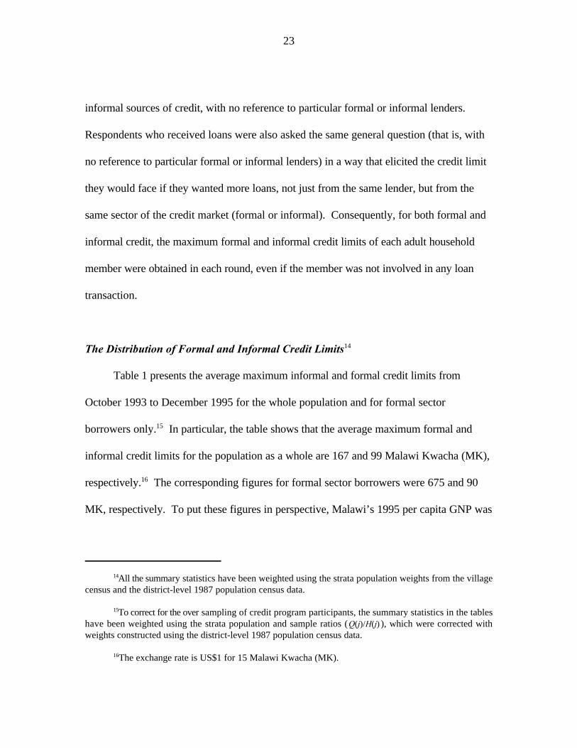
The Distribution of Formal and Informal Credit Limits14

Table 1 presents the average maximum informal and formal credit limits from

October 1993 to December 1995 for the whole population and for formal sector

borrowers only. In particular, the table shows that the average maximum formal and15

informal credit limits for the population as a whole are 167 and 99 Malawi Kwacha (MK),

respectively. The corresponding figures for formal sector borrowers were 675 and 9016

MK, respectively. To put these figures in perspective, Malawi’s 1995 per capita GNP was

24

US$170 (2,550 MK) and the average per capita 1995 income in the sample was 1,190

MK. The box plot diagrams of the distributions presented in Figure 1 give a better

Table 1—Formal and informal credit limits in Malawi (October 1993 to December1995)

All respondents Formal sector borrowers onlyCredit limits Formal Informal Formal Informal

(MK)a

Mean 167 99 675 90

Median 0 40 500 20

Standard deviation 497 354 911 499

Minimum 0 0 13 0

Maximum 10,000 12,000 10,000 12,000

Source: International Food Policy Research Institute and Rural DevelopmentDepartment, Bunda College of Agriculture, Rural Finance Survey, 1995.

US$1 = 15 Malawi Kwacha (MK).a

471471N =

InformalFormal

1000

900

800

700

600

500

400

300

200

100

0

-100

214257 214257N =

FEMALEMALE

1000

900

800

700

600

500

400

300

200

100

0

-100

Formal

Informal

5930 5930N =

FEMALEMALE

2000

1800

1600

1400

1200

1000

800

600

400

200

0

-200

Formal

Informal

5930 5930N =

FEMALEMALE

2000

1800

1600

1400

1200

1000

800

600

400

200

0

-200

Formal

Informal

25Figure 1—Distribution of formal and informal credit limits in Malawi (October 1993 to December 1995): Box plot

diagramsAll Respondents

Formal Sector Borrowers Only

Notes: Box plot diagrams are interpreted as follow: For each box, 50 percent of cases have values within the box and the solid horizontal line insideis the median. The length of the box is the interquartile range and the lower boundary (resp upper boundary) of the box is the 25th(respectively, 75th) percentile. Finally, the circles are outliers and the stars are extreme values. The exchange rate is US$1 = 15 MK. Malawi’s 1995 per capita GNP was US$170 (2,550 MK).

26

picture of the extent of access to credit in Malawi. The figure shows that the median

formal and informal credit limits in the population as a whole are, respectively, zero and

40 MK. Fifty percent of the population can borrow at most 100 MK (less than US$10)

from either sector of the credit market. Formal sector borrowers have a higher median

formal credit limit (375 MK) but a lower median informal credit limit (20 MK). This

likely reflects of the fact that two of the credit programs studied are targeted to poor

women who might have been excluded from the few existing sources of informal credit

because of their socioeconomic situation (see Figure 1).

Household Income

Table 2 shows that the average 1995 per capita total household income in the

survey areas was 1,190 MK for 1995 and 986 MK for 1994. The average per capita crop

income in the drought year of 1994 (161 MK) is half the average crop income for 1995.

This shows the high income risk that agricultural households relying only on crop

production have to face in Malawi. On the other hand, nonfarm income generating

activities, which are presumably less dependent on weather, may be not only a less risky

source of income, but also a substantial source of income for rural households (more than

twice the average crop income). Finally, the average per capita total income of credit

program participants in 1994 (1,559 MK) and 1995 (1,833 MK) is almost twice as high as

that of past participants (756 and 1,017 MK, respectively) and that of households who

never participated in any credit program (856 and 1,025 MK, respectively).

27Table 2—Household per capita incomes, food expenditure, calorie intake, and nutritional status: By credit program

membership

Current members All Mudzi Past Never been

households MRFC Fund MUSCCO PMERW1 PMERW2 Other All members members

Total income (MK)a

1994 986 1,565 1,389 805 1,039 2,844 1,567 1,559 756 8561995 1,190 1,843 1,493 1,471 1,212 4,204 1,978 1,833 1,017 1,025

Crop income (MK)1994 161 155 –76 227 49 249 397 154 166 1611995 365 433 28 893 223 1,608 809 429 427 330

Nonfarm income (1995, MK) 825 1,410 1,465 578 989 2,596 1,170 1,404 590 695

Monthly food expenditure (MK) 129 112 137 104 113 142 173 120 94 140

Daily calorie intake (Kcal) 2,184 1,949 2,168 2,083 1,985 2,094 1,984 1,979 1,901 2,313

Average share of food out of totalconsumption 88% 86% 80% 87% 84% 83% 85% 86% 91% 88%

Average share of food out of totalcash expenditure 71% 75% 73% 64% 75% 76% 74% 74% 71% 70%

Height-for-age–1 s.d. below reference 66% 72% 77% 72% 79% 71% 83% 74% 72% 62%–2 s.d. below reference 46% 55% 49% 53% 58% 45% 43% 53% 61% 39%

Weight-for-age–1 s.d. below reference 46% 55% 40% 49% 45% 37% 60% 52% 51% 42%–2 s.d. below reference 16% 20% 8% 18% 19% 13% 2% 17% 21% 15%

Source: International Food Policy Research Institute/Rural Development Department, Bunda College of Agriculture (IFPRI/RDD), Rural FinanceSurvey, 1995.

Notes: The 1994 nonfarm income information was not collected, but it is assumed to be the same as for 1995. Total food expenditure includes theimputed value of food out of home production. Kcal stands for kilocalories; s.d. for standard deviation.

US$1 = 15 MK.a

28

Household Expenditures and Calorie Intake

Table 2 shows that the average household per capita monthly total expenditure in

the survey areas is 129 MK, with a relatively high share of food in the household monthly

consumption budget (88 percent, including the imputed value of home produced food).

The average per capita daily intake in the sample was 2,184 kilocalories, which is close to

the 2,200 kcal/person/day recommended for Malawi. The average per capita daily calorie

intake of households who never participated in any credit program is higher than that for

any of the participants of the credit programs studied. This suggests that participants may

not be spending their increased income on food; or if they do, they are spending it on

luxurious foods with relatively lower calorie content.

Household Nutritional Status

Table 2 shows that 46 percent of preschoolers in the survey areas are chronically

malnourished as measured by the height-for-age Z-scores and are thus stunted. This is

close to the 48.6 percent figure for children under five years of age found in Malawi's

1992 Demographic and Health Survey. As measured by the weight-for-age Z-scores, 16

percent of preschoolers are acutely malnourished. Finally, households who never

participated in any credit program have the lowest prevalence of chronic malnutrition

among preschoolers (39 percent compared to an average of 53 percent for all participants,

and 61 percent for past participants). However, the weight-for-age figures show only a

slight difference in the prevalence of acute malnutrition between households that never

29

The estimation results for the conditional probability choices are reported and discussed by Diagne17

(1997), who also discusses the estimation procedure in greater detail.

When the instruments are weakly correlated with the endogenous regressors, Staiger and Stock18

(1997) recommend using the Durbin and Basmann tests when testing the exogeneity and overidentificationrestrictions, respectively. The Basmann test uses the Limited Information Maximum Likelihood (LIML)estimates.

participated and participating households as a whole (15 percent and 17 percent

respectively).

MARGINAL EFFECTS OF ACCESS TO CREDIT ON HOUSEHOLD WELFARE

The system of equations (1) through (5) was estimated using the two-stage

methodology outlined in Section 3. The results of the estimation are presented in Tables

3-14. The relevant F statistics and exogeneity and overidentification test statistics are17

also presented for each equation. In particular, the high F statistics for the joint

significance of the lenders’ characteristics (the program dummies) in the formal credit limit

equation (F =50.41) should be noted. On the other hand, the F statistics for the joint3,1505

significance of the informal lenders’ characteristics in the informal credit limit equation is

relatively low (F =3.88). The informal lenders’ characteristics may introduce biases in7,1505

the TSLS estimates of the credit demand equations due to their weak correlations with the

informal credit limit (Staiger and Stock 1997). Furthermore, for both the formal and

informal credit demand equations, The Wu-Hausman and Durbin tests fail to reject the null

hypothesis of exogeneity of the presumed endogenous variables. The overidentifying

restrictions are also rejected by the Basmann test. Under these conditions, it is more18

30

For the credit demand equations, there was not much difference between the TSLS and OLS estimates. There were,19

however, noticeable differences between the TSLS and OLS estimates for the food expenditure and calorie intake equations.

appropriate to estimate the two credit demand equations with OLS. The reported results

are OLS estimates. The reported results for the food expenditure and calorie intake

equations are also OLS estimates, for similar reasons.19

Access to Credit and the Demands for Formal and Informal Credits

In order to focus on the assessment of the effects of access to formal credit on

household welfare and keep the paper short, only results for the credit limits and loan

demands directly relevant to the impact equations are discussed. For a full discussion of

the access and participation equations, see Diagne 1997. In Tables 3 through 6, the

following facts are relevant for the impact assessment:

1. All five credit programs have contributed statistically significantly to the

access their member households have to formal credit. Differences with

noncurrent members range from as low as 20 MK per capita per season for

MRFC to as high as 57 MK per capita per season for PMERW1.

2. The estimated average marginal propensity to borrow out of every additional

MK of formal credit made available (FLOANMAX) is estimated at 0.49 and

is statistically significantly different from both zero and 1 (at the 5 percent

level). Hence, households are on average marginally constrained in their

31

Table 3—Formal credit limit equation (FLOANMAX): Matrix of direct and indirectpartial effects of selected variables

Indirect effect through Direct effect the probability choices Total effect a

Estimated Standard Estimated Standard Estimated StandardIndependent variable coefficient error coefficient error coefficient error

CONSTANT –2,534.62 343.0319 –2,534.62 343.0319MRFCH 19.6259 3.9254 19.6259 3.9254MUDZIH 54.0689 7.6468 54.0689 7.6468MUSCOH 33.7595 6.2161 33.7595 6.2161PMERW1H 56.8125 8.0875 56.8125 8.0875PMERW2H 56.4310 7.7808 56.4310 7.7808WMRFC 2,913.05 309.66 2,913.05 309.66WPROG2 2,928.46 322.59 2,928.46 322.59WDPAST 2,790.41 328.91 2,790.41 328.91FPDEFLT –20.7784 13.8852 –2.7817 0.8726 –23.5600 13.7048DP9495 –10.8881 4.6691 –10.8881 4.6691LANDAREH 7.0622 5.7895 0.4440 0.8846 7.5062 6.0081AGLPAREA 0.2929 0.3149 0.2658 0.0757 0.5587 0.3190TASSETVH 0.0017 0.0033 0.0009 0.0004 0.0026 0.0032LDPASSTH –79.3011 28.5800 15.3997 6.2558 –63.9014 29.9756LVPASSTH –46.0946 34.1626 –7.2518 10.3868 –53.3463 37.0432YYEDUCH –0.0618 2.4691 –0.6180 0.5209 –0.6798 2.4549YYEDUCS 2.4703 2.7511 1.5237 0.5690 3.9940 2.7320POPADL15 –19.6817 5.4872 9.0646 1.5756 –10.6171 5.7452DEPRATIO –90.6065 33.2885 35.7310 7.5305 –54.8756 34.9863AGEH –0.0063 0.5270 –0.0244 0.0977 –0.0307 0.5538MALEHEAD –18.3682 16.3404 5.8149 2.4588 –12.5533 16.5945PVMAIZE 5.9506 4.5373 –1.7266 0.9757 4.2240 4.8009PPTOB95 3.9528 2.9707 –0.0950 0.4106 3.8578 2.9262PVOXEN 0.0062 0.0102 –0.0042 0.0045 0.0020 0.0111PVCATL 0.0341 0.0143 0.0183 0.0037 0.0524 0.0146PVGSHP –0.8954 0.3711 –0.0881 0.0635 –0.9835 0.3691PVCHKD 0.0218 0.0188 –0.0022 0.0026 0.0196 0.0189NWLSBUY 21.7647 7.6705 1.7904 1.2270 23.5552 7.8415DISTFA –4.1433 2.0048 –1.5329 0.2872 –5.6762 2.0243DISTPO 6.7724 2.2097 0.6807 0.1656 7.4531 2.2246DISTPSCH 6.1053 5.9583 6.1053 5.9583DISTTCEN –5.5751 2.2008 –5.5751 2.2008SOUTH –72.9070 47.1576 –72.9070 47.1576

R-squared = 0.20F-stat. (all coefficients): F = 7.38(49,1458)

F-stat for the program dummies: F = 50.41(3,1505)

F-stat for all instruments : F = 9.152(27,1481)

Note: These are the exogenous regressors used as instruments in some of the other equations of the system:WMRFC WPROG2 WPAST PVMAIZE PVCASVA PVBEANS PVVEGFRT PVMEAFSH PVDRINKPVOTHER PPTOB95 PVOXEN PVCATL PVGSHP PVCHKD CDTH3Y CILLAC3Y PHVKM PSVKMNCLWATER NWLSBUY DISTFA DISTPO DISTPSCH DISTTCEN CROPRISK CVGAPYYP.

The column of direct effects corresponds to the estimated coefficients of the variables included in the equations.a

32

Table 4—Informal credit limit equation (ILOANMAX): Estimated coefficients ofselected variables (partial effects)

Partial effect

Independent variable Estimated coefficient Standard error

CONSTANT 88.7567 39.7190RELALEND 0.7911 5.3971SHTRADEL –9.8742 9.5635FARMLEND –7.9653 5.9776MALELEND 10.0884 6.4531RICHLEND 8.4306 10.0360SVLGLEND 8.2313 5.6507NGOLEND 24.5043 9.7688FPDEFLT 2.1497 3.5205DP9495 –4.0459 2.3682LANDAREH 5.9994 2.0169AGLPAREA –0.0779 0.0937TASSETVH –0.0000 0.0005LDPASSTH –26.9211 8.4329LVPASSTH –26.2156 8.4539YYEDUCH 0.8625 0.7060YYEDUCS 0.1897 0.6052POPADL15 –0.9945 1.3143DEPRATIO –17.6419 6.5542AGEH –0.2330 0.1454MALEHEAD –4.3006 3.9398DISTPO –0.6407 0.4969PVMAIZE –1.0145 2.3822PPTOB95 –0.8183 0.4166PVOXEN 0.0052 0.0038PVCATL 0.0039 0.0052PVGSHP –0.0618 0.0541PVCHKD 0.0062 0.0051

R-squared = 0.12F-stat. (all coefficients): F = 3.47(56,1451)

F-stat lender characteristics : F = 3.88a(7,1501)

F-stat for all instruments : F = 2.60b(31,1477)

RELALEND SHTRADEL FARMLEND MALELEND RICHLEND SVLGLEND NGOLEND.a

These are the exogenous regressors used as instruments in some of the other equations of the system:b

RELALEND SHTRADEL FARMLEND MALELEND RICHLEND SVLGLEND NGOLENDPVMAIZE PVCASVA PVBEANS PVVEGFRT PVMEAFSH PVDRINK PVOTHER PPTOB95PVOXEN PVCATL PVGSHP PVCHKD CDTH3Y CILLAC3Y PHVKM PSVKM NCLWATER NWLSBUY DISTFA DISTPO DISTPSCH DISTTCEN CROPRISK CVGAPYYP

33

Table 5—Formal credit demand equation (FLOANVAL): Matrix of direct andindirect partial effects of selected variables

Indirect effect through Direct effect FLOANMAX ILOANMAX Total effect a

Estimated Standard Estimated Standard Estimated Standard Estimated StandardIndependent variable coefficient error coefficient error coefficient error coefficient error

CONSTANT 2.1633 17.2245 2.1633 17.2245FLOANMAX 0.4887 0.0873 0.4887 0.0873ILOANMAX -0.0411 0.0435 -0.0411 0.0435MRFCH 9.5921 2.0898 9.5921 2.0898MUDZIH 26.4259 3.8919 26.4259 3.8919MUSCOH 16.4998 3.0489 16.4998 3.0489PMERW1H 27.7668 4.0558 27.7668 4.0558PMERW2H 27.5804 3.8885 27.5804 3.8885WMRFC 1,423.73 192.06 1423.73 192.06WPROG2 1,431.26 191.69 1431.26 191.69WDPAST 1,363.80 196.57 1363.80 196.57DP9495 13.6721 2.8850 -5.3215 2.1320 0.1662 0.2369 8.5168 3.8359FWEEKDLY -0.7499 1.0541 -0.7499 1.0541FNOCLCND 16.4898 13.2291 16.4898 13.2291IWEEKDLY 4.4648 4.0671 4.4648 4.0671IDUEDATE 63.6118 9.6131 63.6118 9.6131INOCLCND -27.7287 6.5529 -27.7287 6.5529IAMTSTD 0.0597 0.1718 0.0597 0.1718FAMTSTD -0.1085 0.0571 -0.1085 0.0571FPDEFLT -11.5148 7.5773 -0.0883 0.2636 -11.6032 7.5652FAINRATT 2.1165 15.5655 2.1165 15.5655PVMAIZE 4.6982 2.3373 2.0645 2.6874 0.0417 0.1794 6.8043 2.9309PPTOB95 -0.5920 0.6393 1.8855 1.4113 0.0336 0.0463 1.3271 1.6583PSTOB95 6.8688 3.7419 6.8688 3.7419PCFERT95 4.3571 1.7454 4.3571 1.7454PSLMZ95 -0.0203 0.1641 -0.0203 0.1641PSHMZ95 -1.4519 1.1416 -1.4519 1.1416LANDAREH 1.3184 2.1390 3.6686 3.2649 -0.2465 0.2732 4.7405 3.7103AGLPAREA -0.0822 0.0995 0.2731 0.1586 0.0032 0.0066 0.1941 0.1666TASSETVH 0.0007 0.0006 0.0013 0.0018 0.0000 0.0000 0.0020 0.0022LDPASSTH -7.3556 8.5398 1.2315 5.3376 1.1061 1.3246 -37.4811 16.2740LVPASSTH 20.4063 9.5880 -26.0728 21.5138 1.0771 1.3185 -45.4020 23.0834YYEDUCH -1.4005 0.8164 -0.3323 1.2185 -0.0354 0.0638 -1.7682 1.3786YYEDUCS -0.3242 0.6678 1.9520 1.3535 -0.0078 0.0412 1.6201 1.3462POPADL15 -3.0591 2.1362 -5.1890 2.9123 0.0409 0.1085 -8.2073 3.4768DEPRATIO 18.9232 10.6739 -26.8202 18.6753 0.7248 0.8437 -45.0186 20.2506AGEH -0.1029 0.1572 -0.0150 0.2720 0.0096 0.0136 -0.1084 0.2711MALEHEAD 0.6103 4.8669 -6.1354 7.8765 0.1767 0.3420 -5.3483 9.1147DISTFA -2.7742 1.0331 0.0166 0.0412 -2.7576 1.0292DISTPO 3.6427 1.2170 0.0263 0.0388 3.6690 1.2229DISTTCEN -2.7248 1.1966 0.0311 0.0517 -2.6937 1.1873SOUTH 3.4651 7.3878 -35.6329 23.0927 0.7590 1.1775 -31.4088 21.6019

R-squared = 0.33F-stat.(all coefficients): F = 16.40(44,1463)F-stat. for the regressors used as instruments in other equations: F = 1.36(13,1495)Wu-Hausman Chi-squared statistics for exogeneity : x = 0.58 b

(9)Durbin Chi-squared statistics for exogeneity : x = 1.39b

(9)Basmann's Chi-squared statistics for the overidentifying restrictions : x = 49.98c

(60)

The column of direct effects corresponds to the OLS coefficients of the variables included in the equations.a

Endogenous regressors: FLOANMAX ILOANMAX IAMTSTD FAMTSTD CINC94 FGIFTRV CDWAGEb

CWMWAGE CFCWAGE.Instruments tested: WMRFC WPROG2 WPAST RELALEND SHTRADEL FARMLEND MALELEND RICHLENDc

SVLGLEND NGOLEND PVOXEN PVCATL PVGSHP PVCHKD PHVKM PSVKM NCLWATER LATRINENWLSBUY DISTFA DISTPO DISTPSCH DISTTCEN CROPRISK CVGAPYYP.

34

Table 6—Informal credit demand equation (ILOANVAL): Matrix of direct andindirect partial effects of selected variables

Indirect effect through Direct effect FLOANMAX ILOANMAX Total effect a

Estimated Standard Estimated Standard Estimated Standard Estimated StandardIndependent variable coefficient error coefficient error coefficient error coefficient error

CONSTANT 0.0570 2.9869 0.0570 2.9869FLOANMAX -0.0034 0.0019 -0.0034 0.0019ILOANMAX 0.0680 0.0227 0.0680 0.0227MRFCH -0.0677 0.0172 -0.0677 0.0172MUDZIH -0.1865 0.0431 -0.1865 0.0431MUSCOH -0.1165 0.0338 -0.1165 0.0338PMERW1H -0.1960 0.0450 -0.1960 0.0450PMERW2H -0.1947 0.0435 -0.1947 0.0435WMRFC -10.0494 3.0750 -10.0494 3.0750WPROG2 -10.1025 3.0391 -10.1025 3.0391WDPAST -9.6263 3.0359 -9.6263 3.0359DP9495 -0.0731 0.4805 0.0376 0.0213 -0.2751 0.2198 -0.3106 0.4886FWEEKDLY 0.0000 0.0000 0.0813 0.0671 0.1461 0.2931 0.2274 0.2930FNOCLCND -0.1278 0.1597 -0.1278 0.1597IWEEKDLY -1.2613 0.8090 -1.2613 0.8090IDUEDATE 6.5236 2.9264 6.5236 2.9264INOCLCND 1.5294 0.8221 1.5294 0.8221IAMTSTD 19.4587 2.4285 19.4587 2.4285FAMTSTD -0.1046 0.0838 -0.1046 0.0838FPDEFLT 0.0025 0.0036 0.0025 0.0036FAINRATT 1.7213 1.8740 1.7213 1.8740PVMAIZE 0.0001 0.2500 -0.0146 0.0221 -0.0690 0.1594 -0.0834 0.2560PPTOB95 0.0012 0.0523 -0.0133 0.0131 -0.0556 0.0318 -0.0678 0.0612PSTOB95 -0.6294 0.5177 -0.6294 0.5177PCFERT95 -0.0204 0.2696 -0.0204 0.2696PSLMZ95 0.0012 0.0067 0.0012 0.0067PSHMZ95 -0.0163 0.1761 -0.0163 0.1761LANDAREH -0.1317 0.3408 -0.0259 0.0292 0.4079 0.1765 0.2503 0.3205AGLPAREA -0.0193 0.0170 -0.0019 0.0014 -0.0053 0.0059 -0.0265 0.0180TASSETVH 0.0002 0.0002 -0.0000 0.0000 -0.0000 0.0000 0.0002 0.0002LDPASSTH 2.3883 1.1688 0.2204 0.1758 -1.8303 0.6484 0.7785 1.1080LVPASSTH 1.3474 1.2919 0.1840 0.1786 -1.7823 0.6994 -0.2509 1.2871YYEDUCH -0.0265 0.1554 0.0023 0.0087 0.0586 0.0500 0.0345 0.1788YYEDUCS 0.1984 0.1130 -0.0138 0.0104 0.0129 0.0490 0.1975 0.1272POPADL15 -0.3012 0.2459 0.0366 0.0239 -0.0676 0.1092 -0.3322 0.2702DEPRATIO -0.2360 1.3061 0.1893 0.1389 -1.1994 0.6180 -1.2461 1.3453AGEH 0.0151 0.0228 0.0001 0.0019 -0.0158 0.0133 -0.0006 0.0217MALEHEAD 0.1279 0.7859 0.0433 0.0596 -0.2924 0.2976 -0.1212 0.8512DISTFA 0.0196 0.0078 -0.0275 0.0380 -0.0079 0.0384DISTPO -0.0257 0.0103 -0.0436 0.0305 -0.0693 0.0317DISTTCEN 0.0192 0.0144 -0.0515 0.0489 -0.0322 0.0518SOUTH 2.0511 1.1483 0.2515 0.2050 -1.2559 0.8844 1.0467 1.6091

R-squared = 0.35F-stat.(all coefficients): F = 18(44,1463)F-stat. for the regressors used as instruments in other equations: F = 1.14(13,1495)Wu-Hausman Chi-squared statistics for exogeneity : x = 1.02 b

(9)

Durbin Chi-squared statistics for exogeneity : x = 1.12c(9)

Basmann's Chi-squared statistics for the overidentifying restrictions : x = 102.833(60)

The column of direct effects corresponds to the OLS coefficients of the variables included in the equations.a

Endogenous regressors: FLOANMAX ILOANMAX IAMTSTD FAMTSTD CINC94 FGIFTRV CDWAGEb

CWMWAGE CFCWAGEInstruments tested: WMRFC WPROG2 WPAST RELALEND SHTRADEL FARMLEND MALELENDc

RICHLEND SVLGLEND NGOLEND PVOXEN PVCATL PVGSHP PVCHKD PHVKM PSVKM NCLWATERLATRINE NWLSBUY DISTFA DISTPO DISTPSCH DISTTCEN CROPRISK CVGAPYYP.

35

demands for formal credit, but on average would borrow only about half the

amount of any increase in their formal credit limits. Therefore, one of the

restrictions implied by the practice of using loan size to measure impact is not

satisfied.

3. The availability of informal credit (ILOANMAX) has a negative but not

statistically significant effect on the demand for formal credit.

4. For all households, the availability of formal credit induces a small and not

statistically significant reduction in the demand for informal credit. However,

this reduction is much larger for credit program members, with statistically

significant differences with noncurrent members ranging from –0.07 MK for

MRFC to –0.19 MK for PMERW1 per capita per season. At least for credit

program members, one can reject the restriction that formal and informal

credits are not (grossly) substitutable.

5. Finally, the interest rate for formal credit (FAINRATT) does not have any

statistically significant effect on the demands for formal and informal credits.

This suggests that improved access to credit is much more important than its

cost for the study households.

36

Marginal Effect of Access to Formal Credit on Household Incomes

The estimated marginal effects of access to formal and informal credits on crop

income, seasonal nonfarm income, and total household annual income are reported in

Tables 7, 8, and 9. Note first that the direct marginal effects resulting from mere access to

credit, as well as the indirect marginal effects resulting from exercising the option to

borrow, are not statistically different from zero for all three types of income. Both

indirect effects resulting from the substitutability between formal and informal sources of

credit are also not statistically different from zero. As a result, for the average household,

the total marginal effects of access to formal credit on all three types of income, although

positive and quite sizable (+0.5, +2.6, and +0.4 MK, respectively), are not statistically

significantly different from zero. However, the substitution away from informal sources of

credit, made possible by access to formal credit, has a positive and statistically significant

effect on the annual incomes of credit program members.

As shown in Tables 6-8, this beneficial substitution effect results from the negative

correlation between borrowing from informal sources and household crop incomes. The

negative correlation applies also to formal credit. Hence, it is the mere act of borrowing,

whether from informal or formal sources, that has a negative effect on crop incomes. In

contrast, both terms of borrowing are positively correlated with nonfarm income. The

beneficial substitution effect is a mere reflection of the fact that the reduced borrowing

from informal sources makes informal loans play a lesser role in the negative impact that

borrowing in general has on net crop incomes. The negative correlation between

37

Table 7—Annual income equation (THHINC95): Matrix of direct and indirect partial effects of selected variables

Indirect effect through Direct effect FLOANMAX ILOANMAX FLOANVAL ILOANVAL Probability choices Total effect a

Independent Estimated Standard Estimated Standard Estimated Standard Estimated Standard Estimated Standard Estimated Standard Estimated Standardvariable coefficient error coefficient error coefficient error coefficient error coefficient error coefficient error coefficient error

CONSTANT -7552.4 46,148.7 -7,552.4 46,148.4FLOANMAX 1.7125 3.3897 -1.3353 1.7707 0.0563 0.0478 0.4334 2.6699ILOANMAX 6.0580 8.2932 0.1123 0.2287 -1.1095 0.8735 5.0607 8.0223FLOANVAL -2.7321 3.5420 -2.7321 3.5420ILOANVAL -16.3198 11.4295 -16.3198 11.4295MRFCH 33.6085 23.8320 -26.2067 13.1621 1.1049 0.3705 -207.450 303.9841 -198.94 301.2462MUDZIH 92.5909 69.5577 -72.1990 35.0980 3.0441 0.9615 26.8553 702.3767 50.2911 692.0499MUSCOH 57.8117 52.0858 -45.0795 26.2913 1.9006 0.7409 25.5588 549.5803 40.1916 542.3843PMERW1H 97.2891 71.7075 -75.8626 36.3650 3.1985 1.0093 27.0664 734.7088 51.6915 723.9371PMERW2H 96.6358 69.2423 -75.3532 34.8965 3.1770 0.9708 27.0366 704.9439 51.4963 694.6686WMRFC -2,657.6 46,814.3 4,988.4 5,757.6 -3,889.8 3,053.5 164.0 75.1 -1,394.9 45,922.0WPROG -541.5 47,206.6 5,014.8 5,676.2 -3,910.4 2,995.2 164.8 73.8 727.8 46,361.9WPAST 395.1 48,921.0 4,778.4 5,757.3 -3,726.0 3,066.4 157.1 73.6 1,604.6 48,159.6FAINRATT 512.3201 874.0637 -5.7825 63.6319 -28.0907 36.5989 478.4469 846.6599PVMAIZE 64.0917 202.4048 7.2335 24.0318 -6.1458 23.4056 -18.5904 26.1713 1.3617 4.3108 -1.3801 41.1871 46.5706 192.8925PPTOB95 156.7981 75.1249 6.6063 18.0323 -4.9574 7.7758 -3.6259 7.8036 1.1060 1.2167 0.8053 15.2987 156.7324 71.2127LANDAREH 404.4854 242.4733 12.8540 46.1391 36.3444 51.8773 -12.9516 28.2957 -4.0845 5.5917 -1.9882 33.5386 434.6595 218.0339AGLPAREA 15.2382 14.0111 0.9567 2.4403 -0.4717 1.1602 -0.5302 1.1074 0.4332 0.4342 -0.1826 4.9100 15.4436 11.9138YYEDUCH 85.5534 76.7510 -1.1642 8.6112 5.2248 10.3604 4.8309 8.1551 -0.5635 2.8733 -0.7670 16.7683 93.1144 75.9134YYEDUCS 70.3333 69.3534 6.8395 13.7611 1.1490 6.9079 -4.4262 7.2828 -3.2239 2.9348 1.1511 26.8509 71.8228 73.0716POPADL15 -269.028 256.885 -18.1813 27.2841 -6.0247 16.4731 22.4234 22.7010 5.4210 6.3074 3.7471 161.3987 -261.642 183.623DEPRATIO -1,224.9 1,144.0 -93.97 161.06 -106.87 151.9 122.99 128.2 20.33 28.3 -4.081 687.3 -1,286.5 739.6AGEH 10.1027 14.8259 -0.0526 1.9849 -1.4113 2.3429 0.2961 1.2267 0.0101 0.3391 0.1870 2.6957 9.1320 13.8115MALEHEAD -59.4222 448.5843 -21.4970 72.7531 -26.0527 53.4473 14.6123 38.9072 1.9780 12.0697 -20.2237 118.9042 -110.605 444.2657

R-squared = 0.41F-stat.(all coefficients): F = 5.61(42,334)

F-stat. for the regressors used as instruments in other equations: F = 1.30(19,358)

Wu-Hausman Chi-squared statistics for exogeneity : x = 193.8 b(12)

Durbin Chi-squared statistics for exogeneity : x = 240.4b(12)

Basmann's Chi-squared statistics for the overidentifying restrictions : x = 18.35c(48)

The column of direct effects corresponds to the Two-Stage Least Squares coefficients of the variables included in the equations.a

Endogenous regressors: FLOANVAL ILOANVAL CINC94 FLOANMAX ILOANMAX MRFC PROG2 DPAST CDWAGE CWMWAGE CFCWAGE WSL12MHH.b

Instruments: RELALEND SHTRADEL FARMLEND MALELEND RICHLEND SVLGLEND NGOLEND CDTH3Y CILLAC3Y PHVKM PSVKM NCLWATERc

NWLSBUY DISTFA DISTPO DISTPSCH DISTTCEN CVGAPYYP.

38

Table 8—Crop income equation (CINC95): Matrix of direct and indirect partial effects of selected variables



CONSTANT 5,668.8 21,961.7 5,668.8 21,961.7FLOANMAX 0.6779 2.3479 -0.1907 1.0624 0.0198 0.0217 0.5071 1.6000ILOANMAX 5.0084 3.8879 0.0160 0.1262 -0.3908 0.4551 4.6336 3.7975FLOANVAL -0.3902 2.0713 -0.3902 2.0713ILOANVAL -5.7479 6.2788 -5.7479 6.2788MRFCH 13.3050 15.1624 -3.7426 6.8114 0.3892 0.1622 -22.3612 142.6544 -12.4096 141.5905MUDZIH 36.6549 48.8864 10.3107 21.3958 1.0721 0.4860 -66.4203 345.0853 -39.0040 340.3183MUSCOH 22.8866 35.8089 -6.4378 15.9929 0.6694 0.3620 -40.8944 268.1098 -23.7762 264.8002PMERW1H 38.5149 49.8833 10.8339 22.0195 1.1265 0.4999 -70.0143 359.2375 -41.2068 354.6772PMERW2H 38.2563 48.1147 10.7612 21.1909 1.1190 0.4801 -69.5120 345.6370 -40.8980 341.2637WMRFC -7,302.4 22,168.6 1,974.8 3,913.5 -555.5 1,751.7 57.7 37.2 -5,825.3 22,048.3WPROG2 -7,433.4 22,394.0 1,985.2 3,855.1 -558.4 1,724.5 58.0 36.7 -5,948.5 22,304.3WPAST -8,476.3 23,203.2 1,891.7 3,859.6 -532.1 1,734.5 55.3 36.7 -7,061.4 23,218.8FAINRATT 58.1004 518.3794 -0.8258 33.3314 -9.8937 15.2258 47.3809 502.6585PVMAIZE 76.2780 143.4955 2.8636 16.3850 -5.0810 11.0083 -2.6549 15.2518 0.4796 1.9227 5.2557 20.4854 77.1411 140.0515PPTOB95 123.4684 43.6626 2.6153 12.3857 -4.0985 3.4505 -0.5178 4.8337 0.3895 0.5175 0.0218 6.6558 121.8788 42.5656LANDAREH 214.4838 113.2434 5.0886 34.2554 30.0473 23.6012 -1.8496 17.2924 -1.4386 1.9758 -1.5037 15.1473 244.8278 98.9608AGLPAREA 8.4024 6.9292 0.3787 1.6016 -0.3900 0.5142 -0.0757 0.6673 0.1526 0.1973 -0.6359 2.2259 7.8322 5.9261YYEDUCH 15.8527 38.7768 -0.4609 6.1185 4.3195 5.5861 0.6899 3.6749 -0.1985 1.3882 1.6335 8.4209 21.8363 38.8014YYEDUCS 49.3381 37.2588 2.7076 10.9516 0.9499 3.3550 -0.6321 4.0275 -1.1355 1.5530 -4.2999 14.1653 46.9281 38.2710POPADL15 -36.9193 118.9392 -7.1976 18.2925 -4.9808 8.6492 3.2023 13.3346 1.9093 3.3910 -23.8789 74.9911 -67.8650 84.6205DEPRATIO -200.415 511.1822 -37.2018 107.4407 -88.3569 81.6060 17.5651 76.4544 7.1623 13.9748 -92.4618 295.6435 -393.708 355.6040AGEH 4.6730 6.8759 -0.0208 1.2978 -1.1668 1.1021 0.0423 0.5890 0.0036 0.1550 0.0886 1.3805 3.6199 6.6046MALEHEAD 45.0110 213.6800 -8.5102 55.2284 -21.5387 30.3052 2.0868 22.9497 0.6967 5.4566 -10.6262 54.1635 7.1193 210.7278

R-squared = 0.48F-stat.(all coefficients): F = 7.31(42,334)


Wu-Hausman Chi-squared statistics for exogeneity : x = 2,028.6b(12)

Durbin Chi-squared statistics for exogeneity : x = 2,816.2b(12)



Endogenous regressors: FLOANVAL ILOANVAL CINC94 FLOANMAX ILOANMAX MRFC PROG2 DPAST CDWAGE CWMWAGE CFCWAGE WSL12MHH.b

Instruments: RELALEND SHTRADEL FARMLEND MALELEND RICHLEND SVLGLEND NGOLEND CDTH3Y CILLAC3Y PHVKM PSVKM NCLWATERc

NWLSBUY DISTFA DISTPO DISTPSCH DISTTCEN CVGAPYYP.

39

Table 9—Nonfarm seasonal income equation (THHNFINC): Matrix of direct and indirect partial effects of selectedvariables



CONSTANT -2,920.34 19,404.23 -2,920.34 19,404.23FLOANMAX 0.4578 4.4206 2.2593 3.4814 -0.0780 0.0614 2.6391 3.4024ILOANMAX -15.7493 13.7246 -0.1899 0.4905 1.5363 1.2431 -14.4030 12.8875FLOANVAL 4.6226 6.5655 4.6226 6.5655ILOANVAL 22.5966 15.3214 22.5966 15.3214MRFCH 8.9848 28.7866 44.3404 25.4182 -1.5299 0.5782 49.2952 72.3267 101.0905 78.9156MUDZIH 24.7530 90.2768 122.1569 71.4990 -4.2149 1.2827 -68.6763 434.8680 74.0188 427.2315MUSCOH 15.4553 65.8514 76.2721 52.8271 -2.6317 0.9642 -46.7539 328.8014 42.3418 323.8395PMERW1H 26.0091 92.0431 128.3554 74.8116 -4.4287 1.3453 071.4548 443.2866 78.4809 435.2255PMERW2H 25.8344 88.8814 127.4935 72.0223 -4.3990 1.3004 -71.0717 432.9406 77.8572 424.3577WMRFC 2,747.1 19,535.3 1,333.6 7,360.9 6,581.3 5,930.3 -227.1 105.2 10.435.0 19,857.4WPROG2 2,134.7 20,080.4 1,340.6 7,257.9 6,616.2 5,818.0 -228.2 102.3 9,863.3 20.271.0WPAST 3,583.7 18,081.9 1,277.4 7,333.8 6.304.3 5,863.8 -217.5 102.4 10,947.9 18,490.8FAINRATT -43.7343 519.2909 9.7838 109.7342 38.8948 35.5796 4.9442 515.5447LANDAREH 26.7649 153.0652 3.4364 60.1561 -94.4869 86.9998 21.9135 55.5116 5.6554 5.8953 1.5015 14.6926 -35.2153 138.3163AGLPAREA -0.5118 5.9193 0.2558 3.0514 1.2264 1.6560 0.8970 2.2990 -0.5998 0.4885 0.1886 1.8153 1.4562 5.6143YYEDUCH 3.9859 50.3358 -0.3112 9.4988 -13.5832 17.2357 -8.1736 12.4208 0.7802 3.3265 -0.2270 6.6927 -17.5289 46.7126YYEDUCS 0.8894 27.4321 1.8285 15.8710 -2.9870 15.4920 7.4889 13.2780 4.4638 3.9187 1.1860 9.6979 12.8696 25.5860POPADL15 96.8778 121.6048 -4.8605 33.1819 15.6628 30.8281 -37.9392 43.4252 -7.5061 7.9216 5.8635 62.9972 68.0982 102.0560DEPRATIO 331.9313 503.9407 -25.1223 196.6631 277.8476 273.5825 -208.103 250.7025 -28.156 35.7759 27.524 240.8914 375.921 450.9923AGEH -0.7393 6.3068 -0.0141 2.0401 3.6690 3.9147 -0.5009 1.5888 -0.0140 0.3952 -0.1179 1.0155 2.2829 4.8413MALEHEAD -14.5879 229.9565 -5.7470 107.9838 67.7308 79.2852 -24.7233 88.2941 -2.7388 14.9004 5.4384 32.7820 25.3723 174.1397

R-squared = 0.16F-stat.(all coefficients): F = 5.13(40.1090)


Wu-Hausman Chi-squared statistics for exogeneity : x = 676.4b(8)




Endogenous regressors: FLOANVAL ILOANVAL FLOANMAX ILOANMAX MRFC PROG2 DPAST CINC94.b

Instruments: RELALEND SHTRADEL FARMLEND MALELEND RICHLEND SVLGLEND NGOLEND PVOXEN PVCATL PVGSHP PVCHKD.c

40

Note that, as shown in the direct effect columns, the mere access to credit (formal or informal) is20

positively correlated with crop income (and with nonfarm income). It is the exercising of the option to borrowby smallholder farmers that negatively affects their net crop income due to the relatively high input-outputprice ratio.

Note that net crop income includes the cost of the inputs acquired through borrowing even if the21

loans were not repaid. About 20 percent of the sample households had a negative net crop income for the1994/95 season. Furthermore, half of the sample households in one of the district surveyed (Mangochi)experienced a complete crop failure (no harvest).

borrowing and crop income is not surprising. Indeed, gross margin calculations using on-

farm trial data from more than 1,600 sites in Malawi have shown that, even in years of

relatively favorable climatic conditions, growing maize (the major crop in Malawi) is

barely profitable due to the very low price of maize compared to the very high price of

fertilizer (Benson 1997; Msukwa et al. 1994). The very high relative input-output price

ratio, combined with the fact that the 1995 harvest was below average and followed a

severe drought in 1994, explains why, everything else being equal, smallholder farmers

who borrowed to buy inputs experienced lower crop income. Yet, despite the20

unprofitability of maize, the formal loan demand equation suggests that, on average, once

they get access to formal credit, most farmers would not restrain themselves from

borrowing. Moreover, they would respond to higher fertilizer prices by increasing their

demand for formal loans in order to keep the same level of input use (see Diagne 1997).

This type of behavior from smallholder farmers appears irrational unless they expect debt

forgiveness or intend to default and use the unprofitability of maize as an excuse (see

Msukwa et al. 1994).21

For the above reasons, the substitution away from informal sources of credit by

credit program members was beneficial for their crop incomes but detrimental for their

41

Note that crop income includes nonmarketed crop production valued at market prices.22

nonfarm incomes. There were no compensating beneficial effects from the increased

reliance on formal loans. Consequently, after controlling for all other factors, the incomes

of credit program members are still not statistically significantly different from those of

noncurrent members. In fact, from the effects of the credit programs—through the

choice-based-corrected conditional probability choices (shown in all table columns labeled

"Probability choices"), which reflect mostly the self-selection and targeted nature of the

programs—one can infer that with or without the direct and indirect effects of access to

formal credit, the incomes of credit program members are not statistically significantly

different from those of noncurrent members.

Finally, one can see from Table 7 that the two most important determinants of

household annual income are landholding size (LANDAREH, +434.7 MK of additional

income per capita for every additional hectare of land owned) and the producer price of

tobacco (PPTOB95, +156.7 MK of additional income per capita for every MK increase in

the producer price). Moreover, the significant marginal effects of these two factors on

household income occur as a result of their direct effects on crop income. The indirect

effects through household access to credit and borrowing are all statistically insignificant.

In contrast, the price of maize, the major food staple and most important crop in terms of

area planted in Malawi (PVMAIZE), has no statistically significant direct or indirect

effects on household incomes. This suggests that even higher maize prices will fail to22

increase crop income in Malawi if the 1994 and 1995 climatic conditions continue to

42

prevail and smallholders continue to face a severe land constraint. Under the current

situation, the adoption of high-value export crops such as tobacco, combined with terms

of trade for these products that are favorable to farmers, is more likely to have a bigger

impact on per capita incomes in Malawi than a continuous heavy reliance on maize, even

with a substantial increase in its producer price.

Marginal Impact of Access to Credit on Household Food Security

Tables 10, 11, and 12 present the results related to the effects of access to formal

credit on household food security. The tables show several notable findings. First, access

to formal credit has no statistically significant direct effect on per capita household daily

food expenditure (Table 10). The indirect effects (through borrowing, substitution, and

income) are also all negligible and statistically insignificant. The only exception is the

substitution effect for credit program members. However, when all the direct and indirect

effects are added there are no statistically significant differences in per capita food

expenditure between current and noncurrent members of the credit program.

Second, neither the direct nor the indirect effects on calorie and protein intake of

the various channels of access to formal credit (substitution, borrowing, income and food

expenditure) are statistically significantly different from zero (Tables 11 and 12). As a

43

Table 10—Daily food expenditure equation (FOODEXC): Matrix of direct and indirect partial effects of selected variables

Indirect effect through Direct effect FLOANMAX ILOANMAX FLOANVAL ILOANVAL THHINC95 Probability choices a

Total effect Independent Estimated Standard Estimated Standard Estimated Standard Estimated Standard Estimated Standard Estimated Standard Estimated Standard Estimated Standardvariable coefficient error coefficient error coefficient error coefficient error coefficient error coefficient error coefficient error coefficient error

CONSTANT 5.5174 4.8133 0.0000 0.0000 0.0000 0.0000 0.0000 0.0000 0.0000 0.0000 0.0000 0.0000 0.0000 0.0000 1.5174 4.8133FLOANMAX -0.0003 0.0008 0.0000 0.0000 0.0000 0.0000 0.0004 0.0007 0.0000 0.0000 0.0001 0.0004 0.0000 0.0000 0.0002 0.0006ILOANMAX 0.0015 0.0014 0.0000 0.0000 0.0000 0.0000 -0.0000 0.0001 -0.0005 0.0004 0.0006 0.0013 0.0000 0.0000 0.0016 0.0018FLOANVAL 0.0008 0.0013 0.0000 0.0000 0.0000 0.0000 0.0000 0.0000 0.0000 0.0000 -0.0003 0.0006 0.0000 0.0000 0.0005 0.0014ILOANVAL -0.0075 0.0057 0.0000 0.0000 0.0000 0.0000 0.0000 0.0000 0.0000 0.0000 -0.0021 0.0021 0.0000 0.0000 -0.0095 0.0057THHINC95 0.0001 0.0001 0.0000 0.0000 0.0000 0.0000 0.0000 0.0000 0.0000 0.0000 0.0000 0.0000 0.0000 0.0000 0.0001 0.0001MRFCH 0.0000 0.0000 -0.0066 0.0055 0.0000 0.0000 0.0080 0.0050 0.0005 0.0002 -0.0251 0.0480 -0.0532 0.0248 -0.0764 0.0519MUDZIH 0.0000 0.0000 -0.0183 0.0177 0.0000 0.0000 0.0222 0.0145 0.0014 0.0005 0.0063 0.1137 0.0422 0.0741 0.0538 0.1379MUSCOH 0.0000 0.0000 -0.0114 0.0134 0.0000 0.0000 0.0138 0.0111 0.0009 0.0004 0.0051 0.0888 0.0286 0.0573 0.0369 0.1077PMERW1H 0.0000 0.0000 -0.0192 0.0184 0.0000 0.0000 0.0233 0.0152 0.0015 0.0005 0.0065 0.1194 0.0441 0.0766 0.0562 0.1441PMERW2H 0.0000 0.0000 -0.0191 0.0177 0.0000 0.0000 0.0231 0.0145 0.0015 0.0005 0.0065 0.1142 0.0438 0.0739 0.0558 0.1381WMRFC 4.0373 4.9635 -0.9856 1.4378 0.0000 0.0000 1.1944 1.1930 0.0752 0.0377 -0.1761 7.6577 0.0000 0.0000 4.1451 8.9539WPROG2 4.7920 4.9462 -0.9908 1.4225 0.0000 0.0000 1.2007 1.1747 0.0756 0.0373 0.0919 7.7558 0.0000 0.0000 5.1693 9.0173WPAST 5.9827 5.5650 -0.9441 1.4395 0.0000 0.0000 1.1441 1.1858 0.0720 0.0375 0.2025 8.1027 0.0000 0.0000 6.4572 9.6132FAINRATT 0.0000 0.0000 0.0000 0.0000 0.0000 0.0000 0.0018 0.0225 -0.0129 0.0187 0.0604 0.1315 0.0000 0.0000 0.0493 0.1314PVMAIZE -0.0712 0.0903 -0.0014 0.0063 -0.0015 0.0051 0.0057 0.0097 0.0006 0.0028 0.0059 0.0342 -0.0041 0.0041 -0.0660 0.0974PVCASVA -0.0073 0.0646 0.0014 0.0048 0.0039 0.0050 -0.0019 0.0044 0.0006 0.0023 0.0114 0.0406 0.0000 0.0000 0.0080 0.0755PVBEANS 0.0734 0.0279 0.0007 0.0018 -0.0025 0.0024 -0.0008 0.0018 0.0010 0.0009 -0.0104 0.0151 0.0000 0.0000 0.0614 0.0334PVVEGFRT 0.3531 0.0552 -0.0053 0.0134 -0.0040 0.0040 0.0051 0.0098 0.0020 0.0022 0.0158 0.0328 0.0000 0.0000 0.3668 0.0626PVMEAFSH 0.0113 0.0267 0.0010 0.0036 -0.0018 0.0021 -0.0004 0.0024 0.0013 0.0017 0.0029 0.0206 0.0000 0.0000 0.0143 0.0328PVDRINK -0.0008 0.0082 -0.0002 0.0007 -0.0002 0.0004 0.0002 0.0006 -0.0002 0.0004 -0.0033 0.0137 0.0000 0.0000 -0.0045 0.0164LANDAREH 0.1980 0.0699 -0.0025 0.0142 0.0090 0.0086 0.0040 0.0128 -0.0019 0.0032 0.0549 0.0378 0.0004 0.0037 0.2619 0.0755POPADL15 -0.8131 0.0835 0.0036 0.0075 -0.0015 0.0037 -0.0069 0.0112 0.0025 0.0034 -0.0330 0.0348 0.0172 0.0145 -0.8312 0.0887DEPRATIO -4.3464 0.5818 0.0186 0.0496 -0.0264 0.0304 -0.0378 0.0659 0.0093 0.0154 -0.1624 0.1464 0.0607 0.0621 -4.4844 0.5951AGEH 0.0065 0.0068 0.0000 0.0005 -0.0003 0.0005 -0.0001 0.0004 0.0000 0.0002 0.0012 0.0023 -0.0000 0.0004 0.0072 0.0071MALEHEAD 0.3692 0.2404 0.0042 0.0211 -0.0064 0.0112 -0.0045 0.0183 0.0009 0.0079 -0.0140 0.0765 0.0002 0.0110 0.3497 0.2554

R-squared = 0.32F-stat.(all coefficients): F = 13.64(37.1093)





The column of direct effects corresponds to the Ordinary Least Squares coefficients of the variables included in the equations.a

Endogenous regressors: FLOANVAL ILOANVAL THHINC95 FLOANMAX ILOANMAX MRFC PROG2 DPAST CINC94 FGIFTRV CDWAGE CWMWAGE CFCWAGE SINCS95.b

Instruments: RELALEND SHTRADEL FARMLEND MALELEND RICHLEND SVLGLEND NGOLEND FAINRATT PPTOB95 PSTOB95 PCFERT95 PSLMZ95 PSHMZ95 PVOXENc

PVCATL PVGSHP PVCHKD NCLWATER NWLSBUY DISTFA DISTPO DISTPSCH DISTTCEN CROPRISK CVG9495P CVGAPYYP.

44Table 11—Daily calorie intake equation (CALORYC): Matrix of direct and indirect partial effects of selected variables

Indirect effect through Direct effect FLOANMAX ILOANMAX FLOANVAL ILOANVAL THHINC95 FOODEXC Probability choices Total effect a

Independent Estimated Standard Estimated Standard Estimated Standard Estimated Standard Estimated Standard Estimated Standard Estimated Standard Estimated Standard Estimated Standardvariable coefficient error coefficient error coefficient error coefficient error coefficient error coefficient error coefficient error coefficient error coefficient error

CONSTANT 1,937.02 1,048.45 0.0000 0.0000 0.0000 0.0000 0.0000 0.0000 0.0000 0.0000 0.0000 0.0000 0.0000 0.0000 0.0000 0.0000 1,937.02 1,048.45FLOANMAX 0.2395 0.1495 0.0000 0.0000 0.0000 0.0000 -0.1553 0.1220 0.0049 0.0075 0.0073 0.0641 0.0298 0.1195 0.0000 0.0000 0.1263 0.1870ILOANMAX -0.0621 0.3900 0.0000 0.0000 0.0000 0.0000 0.0131 0.0200 -0.0974 0.1300 0.0853 0.2685 0.3119 0.3485 0.0000 0.0000 0.2508 0.6678FLOANVAL -0.3177 0.2640 0.0000 0.0000 0.0000 0.0000 0.0000 0.0000 0.0000 0.0000 -0.0461 0.0932 0.0968 0.2747 0.0000 0.0000 -0.2670 0.4087ILOANVAL -1.4325 1.9838 0.0000 0.0000 0.0000 0.0000 0.0000 0.0000 0.0000 0.0000 -0.2751 0.3781 -1.8687 1.1223 0.0000 0.0000 -3.5763 2.4391THHINC95 0.0169 0.0179 0.0000 0.0000 0.0000 0.0000 0.0000 0.0000 0.0000 0.0000 0.0000 0.0000 0.0247 0.0123 0.0000 0.0000 0.0416 0.0198FOODEXC 195.9134 14.0300 0.0000 0.0000 0.0000 0.0000 0.0000 0.0000 0.0000 0.0000 0.0000 0.0000 0.0000 0.0000 0.0000 0.0000 195.9134 14.0300MRFCH 0.0000 0.0000 4.7011 1.1077 0.0000 0.0000 -3.0476 0.9171 0.0970 0.0547 -3.3540 6.7474 -14.9710 10.1916 -7.7437 6.3301 -24.3182 15.8915MUDZIH 0.0000 0.0000 12.9514 3.7507 0.0000 0.0000 -8.3962 2.8636 0.2672 0.1664 0.8479 18.8042 10.5348 26.7004 -6.8448 18.2449 9.3602 42.8221MUSCOH 0.0000 0.0000 8.0866 2.8922 0.0000 0.0000 -5.2424 2.1834 0.1668 0.1292 0.6776 15.5823 7.2350 20.8735 -4.2715 14.2540 6.6520 34.3723PMERW1H 0.0000 0.0000 13.6086 3.9402 0.0000 0.0000 -8.8222 2.9652 0.2808 0.1738 0.8715 19.3594 11.0068 27.9099 -7.1443 18.8800 9.8011 44.5487PMERW2H 0.0000 0.0000 13.5172 3.8016 0.0000 0.0000 -8.7630 2.8751 0.2789 0.1680 0.8682 18.8562 10.9408 26.7660 -7.1035 18.1871 9.7385 43.0396WMRFC 753.484 1,117.798 697.7762 263.4124 0.0000 0.0000 -452.355 204.5549 14.3959 12.8061 -23.5174 1,240.646 812.0895 1,743.183 0.0000 0.0000 1,801.873 2,796.261WPROG2 833.522 1,120.218 701.4679 263.2344 0.0000 0.0000 -454.749 203.2316 14.4720 12.6689 12.2701 1,264.627 1,012.728 1,758.306 0.0000 0.0000 2,119.712 2,822.899WPAST 1,266.95 1,224.561 668.4025 262.0325 0.0000 0.0000 -433.313 203.0325 13.7899 12.6112 27.0523 1,315.589 1,265.056 1,877.552 0.0000 0.0000 2,807.943 2,997.378FAINRATT 0.0000 0.0000 0.0000 0.0000 0.0000 0.0000 -0.6725 7.8214 -2.4657 4.8241 8.0661 24.4193 9.6568 25.4485 0.0000 0.0000 14.5847 44.3950PVMAIZE -123.422 23.9276 1.0118 1.4970 0.0630 1.0657 -2.1619 1.9707 0.1195 0.6106 0.7851 5.2811 -12.9226 19.0735 -0.8120 1.0546 -137.339 28.3977PVCASVA -55.8158 14.6715 -0.09893 1.1714 -0.1618 1.0216 0.7331 1.0266 0.1112 0.5387 1.5236 6.8858 1.5715 14.6747 0.0000 0.0000 -53.0276 22.4637PVBEANS -18.9885 6.7343 -0.4997 0.5172 0.1050 0.6036 0.2942 0.4817 0.1888 0.2801 -1.3924 2.1735 12.0264 6.5578 0.0000 0.0000 -8.2662 10.3826PVVEGFRT -37.8718 18.0676 3.7612 2.8305 0.1650 1.0234 -1.9387 2.3998 0.3912 0.7650 2.1140 4.4157 71.8666 13.7271 0.0000 0.0000 38.4874 22.0776PVMEAFSH -6.6562 7.0132 -0.6903 0.7057 0.0734 0.4510 0.1660 0.5270 0.2537 0.4510 0.3861 2.9983 2.7948 6.3651 0.0000 0.0000 -3.6725 10.5964PVDRINK 4.0941 2.1142 0.1246 0.1526 0.0078 0.0761 -0.0807 0.1282 -0.0434 0.0979 -0.4403 2.0669 -0.8855 3.1757 0.0000 0.0000 2.7766 5.0207LANDAREH -27.3749 15.8647 1.7980 2.4239 -0.3723 2.3598 -1.5062 2.3434 -0.3585 0.8475 7.3279 8.1515 51.3041 15.6957 0.2077 0.9857 31.0258 23.2492POPADL15 -167.215 17.3910 -2.5432 1.9017 0.0617 0.6862 2.6077 2.1122 0.4758 0.9755 -4.4110 6.1550 -162.846 20.1677 2.9799 3.3226 -330.890 24.7581DEPRATIO -811.307 110.3291 -13.1446 9.5763 1.0948 7.3671 14.3035 10.1402 1.7850 4.0843 -21.6899 22.9986 -878.554 130.9740 10.7981 14.9665 -1,696.71 165.8463AGEH 3.7934 1.7908 -0.0074 0.1412 0.0145 0.1231 0.0344 0.1200 0.0009 0.0483 0.1540 0.4261 1.4198 1.3673 -0.0117 0.0895 5.3979 2.4247MALEHEAD 21.7985 68.3557 -3.0069 4.9294 0.2669 2.3507 1.6993 4.0974 0.1736 2.1342 -1.8647 12.2920 68.5142 50.3749 -0.1028 2.7056 87.4781 91.4149

R-squared = 0.26

F-stat.(all coefficients): F = 10.19(38.1092)





The column of direct effects corresponds to the Ordinary Least Squares coefficients of the variables included in the equations.a

Endogenous regressors: FLOANVAL ILOANVAL THHINC95 FOODEXC FLOANMAX ILOANMAX MRFC PROG2 DPAST CINC94 FGIFTRV CDWAGE CWMWAGE CFCWAGEb

SINCS95.Instruments: RELALEND SHTRADEL FARMLEND MALELEND RICHLEND SVLGLEND NGOLEND FAINRATT PPTOB95 PSTOB95 PCFERT95 PSLMZ95 PSHMZ95 PVOXENc


45Table 12—Daily protein intake equation (PROTEINC): Matrix of direct and indirect partial effects of selected variables

Indirect effect through Direct effect FLOANMAX ILOANMAX FLOANVAL ILOANVAL THHINC95 FOODEXC Probability choices Total effect a

Independent Estimated Standard Estimated Standard Estimated Standard Estimated Standard Estimated Standard Estimated Standard Estimated Standard Estimated Standard Estimated Standardvariable coefficient error coefficient error coefficient error coefficient error coefficient error coefficient error coefficient error coefficient error coefficient error

CONSTANT -92.4470 166.0262 0.0000 0.0000 0.0000 0.0000 0.0000 0.0000 0.0000 0.0000 0.0000 0.0000 0.0000 0.0000 0.0000 0.0000 -92.4470 166.0262FLOANMAX 0.1074 0.1318 0.0000 0.0000 0.0000 0.0000 -0.0815 0.1040 0.0000 0.0014 -0.0032 0.0171 0.0019 0.0067 0.0000 0.0000 0.0246 0.0483ILOANMAX -0.1451 0.3020 0.0000 0.0000 0.0000 0.0000 0.0069 0.0123 -0.0003 0.0273 -0.0374 0.0523 0.0194 0.0206 0.0000 0.0000 -0.1566 0.2827FLOANVAL -0.1668 0.1911 0.0000 0.0000 0.0000 0.0000 0.0000 0.0000 0.0000 0.0000 0.0202 0.0239 0.0060 0.0163 0.0000 0.0000 -0.1406 0.1896ILOANVAL -0.0048 0.3772 0.0000 0.0000 0.0000 0.0000 0.0000 0.0000 0.0000 0.0000 0.1206 0.0999 -0.1164 0.0806 0.0000 0.0000 -0.0006 0.3664THHINC95 -0.0074 0.0052 0.0000 0.0000 0.0000 0.0000 0.0000 0.0000 0.0000 0.0000 0.0000 0.0000 0.0015 0.0010 0.0000 0.0000 -0.0058 0.0050FOODEXC 12.2026 3.7080 0.0000 0.0000 0.0000 0.0000 0.0000 0.0000 0.0000 0.0000 0.0000 0.0000 0.0000 0.0000 0.0000 0.0000 12.2026 3.7080MRFCH 0.0000 0.0000 2.1081 0.9818 0.0000 0.0000 -1.5997 0.7761 0.0003 0.0105 1.4701 1.8854 -0.9325 0.6586 2.0373 1.3134 3.0836 2.0212MUDZIH 0.0000 0.0000 5.8077 2.4690 0.0000 0.0000 -4.4071 1.8546 0.0009 0.0292 -0.3716 4.2578 0.6562 1.6303 2.4327 3.0374 4.1187 4.7127MUSCOH 0.0000 0.0000 3.6262 1.8653 0.0000 0.0000 -2.7517 1.3732 0.0006 0.0223 -0.2970 3.2499 0.4506 1.2867 1.4624 2.3773 2.4911 3.6557PMERW1H 0.0000 0.0000 6.1024 2.5702 0.0000 0.0000 -4.6308 1.8867 0.0009 0.0305 -0.3820 4.4027 0.6856 1.7208 2.5658 3.1390 4.3420 4.8792PMERW2H 0.0000 0.0000 6.0614 2.4629 0.0000 0.0000 -4.5997 1.8134 0.0009 0.0294 -0.3805 4.2053 0.6815 1.6392 2.5473 3.0391 4.3109 4.6910WMRFC 209.923 166.9032 312.8968 216.5914 0.0000 0.0000 -237.440 164.5999 0.0485 2.4180 10.3078 291.6821 50.5814 108.1826 0.0000 0.0000 346.3178 323.9520WPROG2 200.857 164.3553 314.5522 212.8646 0.0000 0.0000 -238.696 161.0225 0.0488 2.3687 -5.3781 293.3134 63.0784 109.2879 0.0000 0.0000 334.4615 322.3594WPAST 207.591 189.8214 299.7250 217.8854 0.0000 0.0000 -227.445 164.9746 0.0465 2.3653 -11.8572 305.6325 78.7947 116.9142 0.0000 0.0000 346.8549 351.5252FAINRATT 0.0000 0.0000 0.0000 0.0000 0.0000 0.0000 -0.3530 2.7272 -0.0083 0.8177 -3.5354 5.8876 0.6015 1.5405 0.0000 0.0000 -3.2952 5.5898PVMAIZE -4.1229 2.1401 0.4537 1.0392 0.1472 0.6804 -1.1348 1.4873 0.0004 0.0974 -0.3441 1.4950 -0.8049 1.0942 -0.1224 0.1701 -5.9278 2.5010PVCASVA -4.9982 2.6720 -0.4436 0.7307 -0.3783 0.8718 0.3848 0.5831 0.0004 0.0868 -0.6678 1.4249 0.0979 0.8443 0.0000 0.0000 -6.0049 3.0035PVBEANS -1.4044 0.8068 -0.2241 0.3538 0.2455 0.5029 0.1544 0.2571 0.0006 0.0491 0.6103 0.6319 0.7491 0.4401 0.0000 0.0000 0.1314 0.8806PVVEGFRT -2.5892 2.4929 1.6866 2.0296 0.3858 0.8805 -1.0176 1.2112 0.0013 0.1418 -0.9266 1.2943 4.4762 1.6048 0.0000 0.0000 2.0164 2.2130PVMEAFSH -0.9739 0.7201 -0.3095 0.4051 0.1717 0.3460 0.0871 0.2346 0.0009 0.0838 -0.1692 0.7708 0.1741 0.3838 0.0000 0.0000 -1.0189 1.0014PVDRINK -0.1183 0.2385 0.0559 0.0995 0.0182 0.0562 -0.0424 0.0671 -0.0001 0.0158 0.1930 0.6127 -0.0552 0.1906 0.0000 0.0000 0.0511 0.5713LANDAREH 0.9278 2.8644 0.8063 1.6800 -0.8707 1.9410 -0.7906 1.4426 -0.0012 0.1376 -3.2118 2.1744 3.1955 1.3267 0.0465 0.1558 0.1017 1.8728POPADL15 -5.2861 3.2965 -1.1404 0.9289 0.1443 0.5373 1.3688 1.2657 0.0016 0.1783 1.9334 1.7234 -10.1430 3.1868 0.6054 0.5117 -12.5160 3.1464DEPRATIO -34.7834 17.0598 -5.8943 6.2932 2.5604 6.0732 7.5079 7.2697 0.0060 0.7371 9.5068 6.7419 -54.7212 17.3090 2.4638 2.2642 -73.3541 15.5035AGEH 0.1257 0.1949 -0.0033 0.0732 0.0338 0.0904 0.0181 0.0521 0.0000 0.0072 -0.0675 0.0962 0.0884 0.0857 -0.0031 0.0143 0.1921 0.2054MALEHEAD -4.6434 8.7951 -1.3484 3.5306 0.6241 1.8751 0.8920 2.6718 0.0006 0.3268 0.8173 2.8234 4.2674 3.0297 0.4402 0.4956 1.0498 8.3412

R-squared = 0.21







Endogenous regressors: FLOANVAL ILOANVAL THHINC95 FOODEXC FLOANMAX ILOANMAX MRFC PROG2 DPAST CINC94 FGIFTRV CDWAGE CWMWAGE CFCWAGEb

SINCS95.Instruments: RELALEND SHTRADEL FARMLEND MALELEND RICHLEND SVLGLEND NGOLEND FAINRATT PPTOB95 PSTOB95 PCFERT95 PSLMZ95 PSHMZ95 PVOXENc


46

Tables 10-12 show that mere access to formal credit, as measured by the credit limit variable23

FLOANMAX, has direct positive effects on both calorie and protein intake, although the effects are notstatistically significant.

result, the overall marginal effect of access to formal credit on the food security of the

average household is not statistically significantly different from zero. However,

everything else being equal, mere access to formal credit has significantly higher effects on

food security for credit program members as compared to noncurrent members. Likewise,

the substitution away from informal sources of credit appears to significantly improve the

protein intake of credit program members as compared to noncurrent members. But,

when credit program members exercise the option to borrow from the formal sector, they

end up being significantly worse off. Again, as with income, the mere act of borrowing

(not just from formal sources) is negatively correlated with both calorie and protein intake.

This explains why the reduction in borrowing from informal sources has a positive impact

on household food security, while increased borrowing from formal sources has the

opposite effect. When all the direct and indirect effects of membership in credit23

programs are added (including the effects of self-selection and targeted nature of the

programs), there appear to be no statistically significant differences between the level of

food security of credit program members and that of noncurrent members. There are two

possible explanations for the negative correlation between borrowing and food security as

measured by calorie and protein intake. The first explanation arises from the negative

correlation between borrowing and crop income. Everything else being equal, this

negative correlation should lead to lower calorie intake, especially if smallholders have to

repay the loan. The second possible explanation is that if the loan granted is not enough

47

for the intended investment, the household may reduce food consumption in order to make

up for the shortfall.

Third, Tables 11 and 12 show that, as expected, the most important determinant of

household food security is per capita daily food expenditure (FOODEXC, 195.9 and 12.2

for calorie and protein intakes, respectively). Once daily per capita food expenditure is

controlled for, the only other variables with important and statistically significant overall

effects on per capita daily calorie and protein intakes are the price of maize (PVMAIZE,

–137 and –5.9, respectively) and the price of cassava (PVCASVA, –53 and –6,

respectively). Furthermore, these negative effects of maize and cassava prices are due

mostly to their direct negative impact on both daily calorie and protein intakes. The

indirect effects through the various channels (access to credit, borrowing, income, and

food expenditure) are not statistically different from zero. Maize and cassava are the two

most important food staples in Malawi and together they occupy more than 80 percent of

the country’s cultivated land. Therefore, because of the nonseparability between the food

consumption and production decisions of agricultural households (Singh, Squire, and

Strauss 1986), one should expect maize and cassava prices to have direct effects on

calorie and protein intakes in addition to their indirect effects through the household food

budget. The prices of beans (PVBEANS) and vegetables and fruits (PVVGFRT) also

have statistically significant direct negative effects on calorie and protein intakes for

similar reasons. For the same inseparability reasons, total household income should also

have a direct positive effect on both calorie and protein intakes. However, only its indirect

effects through the household food budget are statistically significant. Furthermore, its

48

overall total effect is statistically significant only for calorie intake. Finally, a larger

household adult population size and higher dependency ratios have negative and

statistically significant effects on household food security.

Marginal Effect of Access to Credit on the Nutritional Status of Children

The effects of access to formal credit on the nutritional status of preschoolers, as

measured by their weight-for-age and height-for-age Z-scores, are presented in Tables 13

and 14. The weight-for-age Z-score measures short-term or acute malnutrition, while the

height-for-age Z-score measures chronic malnutrition. The results are broadly in

agreement with the ones for food security, except for a few exceptions: for both measures

of malnutrition, the direct and indirect effects of access to formal credit are not statistically

significantly different from zero for preschoolers living in the average household.

However, everything else being equal, mere access to formal credit appears to induce

statistically significant positive effects (the more positive the better) on the nutrition of

preschoolers in credit program member households as compared to those in noncurrent

member households. (The only exceptions are MRFC member households.) When the

option to borrow is exercised, preschoolers in credit program member households (except

the ones in MRFC households) end up having significantly worse chronic malnutrition,

compared to those in noncurrent member households. Furthermore,

49

Table 13—Weight-for-age equation (WFAGEZ): Matrix of direct and indirect partial effects of selected variables

Indirect effect through Direct effect FLOANMAX ILOANMAX FLOANVAL ILOANVAL THHINC95 CalorieC PORTEINC Probability choices Total effect a

Independent Est. Standard Est. Standard Est. Standard Est. Standard Est. Standard Esti. Standard Est. Standard Est. Standard Est. Standard Est. Standardvariable coeffi. error coeffi. error coeffi. error coeffi. error coeffi. error coeffi. error coeffi. error coeffi. error coeffi. error coeffi. error

CONSTANT -1.1854 8.7565 0.0000 0.0000 0.0000 0.0000 0.0000 0.0000 0.0000 0.0000 0.0000 0.0000 0.0000 0.0000 0.0000 0.0000 0.0000 0.0000 -1.1854 8.7565FLOANMAX -0.0022 0.0040 0.0000 0.0000 0.0000 0.0000 -0.0001 0.0034 -0.0001 0.0001 0.0001 0.0006 0.0000 0.0002 0.0001 0.0007 0.0000 0.0000 0.0024 0.0025ILOANMAX -0.0108 0.0077 0.0000 0.0000 0.0000 0.0000 0.0000 0.0004 0.0018 0.0015 0.0008 0.0023 0.0000 0.0005 0.0004 0.,0047 0.0000 0.0000 -0.0077 0.0086FLOANVAL -0.0002 0.0070 0.0000 0.0000 0.0000 0.0000 0.0000 0.0000 0.0000 0.0000 -0.0004 0.0008 -0.0000 0.0003 0.0003 0.0026 0.0000 0.0000 -0.0003 0.0076ILOANVAL 0.0264 0.0201 0.0000 0.0000 0.0000 0.0000 0.0000 0.0000 0.0000 0.0000 -0.0027 0.0034 -0.0002 0.0030 0.0000 0.0049 0.0000 0.0000 0.0236 0.0196THHINC95 0.0002 0.0002 0.0000 0.0000 0.0000 0.0000 0.0000 0.0000 0.0000 0.0000 0.0000 0.0000 0.0000 0.0000 0.0000 0.0001 0.0000 0.0000 0.0002 0.0002CalorieC 0.0000 0.0000 0.0000 0.0000 0.0000 0.0000 0.0000 0.0000 0.0000 0.0000 0.0000 0.0000 0.0096 0.1377 -0.0292 0.1463 0.0000 0.0000 -0.0196 0.0944PROTEINC 0.0000 0.0007 0.0000 0.0000 0.0000 0.0000 0.0000 0.0000 0.0000 0.0000 0.0000 0.0000 0.0000 0.0000 0.0000 0.0000 0.0000 0.0000 0.0000 0.0007MRFCH -0.0024 0.0129 0.0000 0.0000 0.0000 0.0000 0.0000 0.0000 0.0000 0.0000 0.0000 0.0000 0.0000 0.0000 0.0000 0.0000 0.0000 0.0000 -0.0024 0.0129MUDZIH 0.0000 0.0000 -0.0435 0.0274 0.0000 0.0000 -0.0020 0.0247 -0.0018 0.0005 -0.0324 0.0606 -0.0012 0.0144 -0.0074 0.0282 -0.0225 0.0572 -0.1108 0.0900MUSCOH 0.0000 0.0000 -0.1199 0.0818 0.0000 0.0000 -0.0056 0.0691 -0.0049 0.0016 0.0082 0.1549 0.0005 0.0295 -0.0099 0.0768 0.0298 0.1392 -0.1018 0.1951PMERW1H 0.0000 0.0000 -0.0749 0.0652 0.0000 0.0000 -0.0035 0.0550 -0.0031 0.0012 0.0065 0.1250 0.0003 0.0232 -0.0060 0.0603 0.0199 0.1118 -0.0607 0.1570PMERW2H 0.0000 0.0000 -0.1260 0.0867 0.0000 0.0000 -0.0059 0.0732 -0.0052 0.0016 0.0084 0.1614 0.0005 0.0304 -0.0104 0.0789 0.0312 0.1454 -0.1074 0.2024WMRFC 0.0000 0.0000 -0.1251 0.0831 0.0000 0.0000 -0.0058 0.0701 -0.0051 0.0016 0.0084 0.1556 0.0005 0.0293 -0.0103 0.0762 0.0310 0.1403 -0.1066 0.1953WPROG2 1.2571 8.6045 -6.4594 6.8822 0.0000 0.0000 -0.3018 5.9161 -0.2656 0.1182 -0.2270 10.2426 0.0883 2.0823 -0.8296 5.3243 0.0000 0.0000 -6.7380 13.6900WPAST 1.5854 8.5201 -6.4936 6.7912 0.0000 0.0000 -0.3034 5.8175 -0.2670 0.1172 0.1185 10.4367 0.1039 2.2038 -0.8012 5.2976 0.0000 0.0000 -6.0574 13.7584

1.7396 9.1971 -6.1875 6.8691 0.0000 0.0000 -0.2891 5.9042 -0.2544 0.1166 0.2612 10.9360 0.1377 2.5604 -0.8309 5.6527 0.0000 0.0000 -5.4235 15.0258

R-squared = 0.13





Note: Est. coeffi. = estimated coefficient.


Endogenous regressors: FLOANVAL ILOANVAL THHINC95 CALORYC PROTEINC FLOANMAX ILOANMAX MRFC PROG2 DPAST CINC94 FGIFTRV CDWAGE CWMWAGE CFCWAGE SINCS95 CDTH3Yb

CILLAC3Y WSL12MHH.

Instruments: PVMAIZE PVCASVA PVBEANS PVVEGFRT PVMEAFSH PVDRINK PVOTHER RELALEND SHTRADEL FARMLEND MALELEND RICHLEND SVLGLEND NGOLEND FAINRATT PPTOB95c

PSTOB95 PCFERT95 PSLMZ95 PSHMZ95 PVOXEN PVCATL PVGSHP PVCHKD NWLSBUY DISTFA DISTPO DISTPSCH DISTTCEN CROPRISK CVG9495P CVGAPYYP.

50

Table 14—Height-for-age equation (HFAGEZ): Matrix of direct and indirect partial effects of selected variables

Indirect effect through Direct effect FLOANMAX ILOANMAX FLOANVAL ILOANVAL THHINC95 CalorieC PORTEINC Probability choices Total effect a

Independent Est. Standard Est. Standard Est. Standard Est. Standard Est. Standard Esti. Standard Est. Standard Est. Standard Est. Standard Est. Standardvariable coeffi. error coeffi. error coeffi. error coeffi. error coeffi. error coeffi. error coeffi. error coeffi. error coeffi. error coeffi. error

CONSTANT -19.6124 12.0794 0.0000 0.0000 0.0000 0.0000 0.0000 0.0000 0.0000 0.0000 0.0000 0.0000 0.0000 0.0000 0.0000 0.0000 0.0000 0.0000 -19.6124 12.0794FLOANMAX 0.0088 0.0063 0.0000 0.0000 0.0000 0.0000 -0.0086 0.0054 0.0000 0.0001 0.0000 0.0009 0.0003 0.0003 -0.0005 0.0011 0.0000 0.0000 0.0000 0.0033ILOANMAX 0.0114 0.0106 0.0000 0.0000 0.0000 0.0000 0.0007 0.0007 -0.0006 0.0016 0.0002 0.0031 0.0005 0.0009 0.0035 0.0066 0.0000 0.0000 0.0158 0.0118FLOANVAL -0.0175 0.0109 0.0000 0.0000 0.0000 0.0000 0.0000 0.0000 0.0000 0.0000 -0.0001 0.0014 -0.0006 0.0005 0.0031 0.0042 0.0000 0.0000 -0.0150 0.0118ILOANVAL -0.0084 0.0227 0.0000 0.0000 0.0000 0.0000 0.0000 0.0000 0.0000 0.0000 -0.0007 0.0058 -0.0074 0.0056 0.0000 0.0087 0.0000 0.0000 -0.0164 0.0228THHINC95 0.0000 0.0003 0.0000 0.0000 0.0000 0.0000 0.0000 0.0000 0.0000 0.0000 0.0000 0.0000 0.0001 0.0000 0.0001 0.0001 0.0000 0.0000 0.0003 0.0003CalorieC 0.0000 0.0000 0.0000 0.0000 0.0000 0.0000 0.0000 0.0000 0.0000 0.0000 0.0000 0.0000 0.4059 0.2185 -0.2726 0.2119 0.0000 0.0000 0.1334 0.1433PROTEINC 0.0021 0.0011 0.0000 0.0000 0.0000 0.0000 0.0000 0.0000 0.0000 0.0000 0.0000 0.0000 0.0000 0.0000 0.0000 0.0000 0.0000 0.0000 0.0021 0.0011MRFCH -0.0223 0.0185 0.0000 0.0000 0.0000 0.0000 0.0000 0.0000 0.0000 0.0000 0.0000 0.0000 0.0000 0.0000 0.0000 0.0000 0.0000 0.0000 -0.0223 0.0185MUDZIH 0.0000 0.0000 0.1726 0.0387 0.0000 0.0000 -0.1680 0.0332 0.0006 0.0006 -0.0083 0.1037 -0.0504 0.0258 -0.0689 0.0438 0.0448 0.0827 -0.0777 0.1304MUSCOH 0.0000 0.0000 0.4754 0.1392 0.0000 0.0000 -0.4629 0.1191 0.0016 0.0015 0.0021 0.2056 0.0194 0.0456 -0.0920 0.1227 0.0432 0.1933 -0.0133 0.2852PMERW1H 0.0000 0.0000 0.2968 0.1079 0.0000 0.0000 -0.2890 0.0912 0.0010 0.0012 0.0017 0.1628 0.0138 0.0364 -0.0556 0.0945 0.0228 0.1528 -0.0087 0.2279PMERW2H 0.0000 0.0000 0.4995 0.1474 0.0000 0.0000 -0.4864 0.1262 0.0016 0.0016 0.0021 0.2155 0.0203 0.0472 -0.0970 0.1274 0.0464 0.1996 -0.0134 0.2972WMRFC 0.0000 0.0000 0.4961 0.1414 0.0000 0.0000 -0.4831 0.1210 0.0016 0.0016 0.0021 0.2063 0.0202 0.0458 -0.0963 0.1232 0.0459 0.1931 -0.0134 0.2858WPROG2 14.7045 11.8173 25.6118 10.9543 0.0000 0.0000 -24.9390 9.4233 0.0839 0.1287 -0.0579 15.4291 3.7335 3.5840 -7.7360 8.7209 0.0000 0.0000 11.4008 18.7896WPAST 14.5745 11.5263 25.7473 10.8101 0.0000 0.0000 -25.0709 9.2941 0.0844 0.1263 0.0302 15.3982 4.3920 3.7925 -7.4711 8.7532 0.0000 0.0000 12.2864 18.7082

17.7437 12.6775 24.5336 10.7491 0.0000 0.0000 -23.8891 9.2587 0.0804 0.1272 0.0666 16.3630 5.8180 4.4831 -7.7480 9.3107 0.0000 0.0000 16.6053 20.3844

R-squared = 0.11





Note: Est. coeffi. = estimated coefficient.


Endogenous regressors: FLOANVAL ILOANVAL THHINC95 CALORYC PROTEINC FLOANMAX ILOANMAX MRFC PROG2 DPAST CINC94 FGIFTRV CDWAGE CWMWAGE CFCWAGE SINCS95 CDTH3Yb

CILLAC3Y WSL12MHH.

Instruments: PVMAIZE PVCASVA PVBEANS PVVEGFRT PVMEAFSH PVDRINK PVOTHER RELALEND SHTRADEL FARMLEND MALELEND RICHLEND SVLGLEND NGOLEND FAINRATT PPTOB95c

PSTOB95 PCFERT95 PSLMZ95 PSHMZ95 PVOXEN PVCATL PVGSHP PVCHKD NWLSBUY DISTFA DISTPO DISTPSCH DISTTCEN CROPRISK CVG9495P CVGAPYYP.

51

However, given the reduced form nature of the estimated equations, one must be cautious with the24

causal interpretations given here. The negative correlation can be consistent with households borrowing moreto take care of their children, when the nutritional status of the children is deteriorating.

because of the positive correlation between informal borrowing and short-term nutrition

levels, credit program members’ substitution away from informal credit leads to a

significant deterioration in the short-term nutritional status of their preschoolers,

compared to the status of noncurrent member households. Finally, as with food security,24

when all the direct and indirect effects of membership in credit programs are added

(including the effects of self-selection and the targeted nature of the programs), there

appears to be no statistically significant differences in the acute and chronic malnutrition of

preschoolers in credit program member and noncurrent member households.

5. CONCLUSION

The estimated marginal effects of either the amount of credit received or

membership in a credit program are not valid measures of the effect of access to credit on

household welfare. This paper has shown how the concept of maximum credit provides

an alternative and more satisfactory framework for measuring the impact of access to

credit. Various direct and indirect effects on household incomes, food security, and

nutritional status of preschoolers have been estimated by applying the maximum credit

framework to data collected in Malawi. The main findings show that, while access to

formal credit enables households to reduce their borrowing from informal sources and

thereby experience marginally beneficial effects on household annual income, these effects

are too small to cause any significant difference between the per capita incomes, food

52

The average length of membership at the time of the survey was less than 3 years.25

security, and nutritional status of credit program members and those of noncurrent

members. Furthermore, this beneficial substitution effect reflects only the fact that

reduced borrowing from informal sources makes informal loans play a lesser role in the

negative effect that borrowing (from formal or informal sources) has on net crop incomes.

The marginal effects on household farm and nonfarm incomes that result from mere access

to formal credit are positive and quite sizable, but not statistically significantly different

from zero.

That credit program members have not yet benefitted from access to formal credit

may be due to the fact that they have not been members for a long enough period. The25

below-average 1995 harvest that followed a severe drought in 1994 should also be kept in

mind. However, the most likely cause of the lack of positive effect of access to formal

credit on household welfare is the unfavorable terms of trade for the farm products of

smallholders. Indeed, gross margin calculations using on-farm trial data have shown that

even in relatively favorable climatic conditions, growing maize is barely profitable due to

the very low relative price of maize and fertilizer (Benson 1997; and Msukwa et al. 1994).

In fact, according to Benson (1997, 14), “...under current prices the use of fertilizer on

hybrid maize in Malawi cannot be recommended for virtually all of the country.” Yet,

despite the unprofitability of maize, the formal loan demand equation suggests that, on

average, once they get access to formal credit, most farmers would not restrain themselves

from borrowing. However, the finding that the price of tobacco has a significant and

53

The average household size in the sample is 5.26

much bigger impact on income than the price of maize, suggests that, instead of maize,

farmers should be devoting more of their scarce resources to tobacco if they want to see a

significant increase in their incomes.

Land scarcity remains the most constraining factor for increasing per capita

household incomes in Malawi. Access to formal credit may not have had positive effects

because of the severe land constraint. The main conclusion drawn from this analysis is

that the necessary complementary resources and economic environment are not yet in

place for access to formal credit to realize its full potential benefits for Malawi’s rural

population. Therefore, policy reforms should emphasize a more equitable land distribution

to ease the land constraints facing smallholder farmers, and should encourage an efficient

and sustainable use of existing cultivable land. However, one must recognize the possible

limitation of land reforms in alleviating the land constraint. More than 80 percent of the

cultivable land in Malawi is already being farmed under the customary tenure system by

smallholder households with an average landholding of 1.1 hectares. Furthermore, 55

percent of these farms are less than 1 hectare each and 95 percent are less than 3 hectares

(World Bank 1987). Therefore, it is doubtful that land reform can significantly alleviate26

the land constraint facing the smallholder, because reform would be limited to the

remaining 20 percent of cultivable land in the hands of large estate holders. Given the

limited scope for land reform, policy reforms should put more emphasis on promoting the

adoption of high-value export crops such as tobacco, and work toward terms of trade for

54

these products that are favorable to farmers. Such policy reforms are more likely to have

a bigger effect on rural poverty and food insecurity in Malawi than a continuous heavy

reliance on maize, even with a substantial increase in its producer price.

p(y|x) 'j

J

j'1

H(j)Q(j)

p(j|x)p(y|x,j)

jJ

j'1

H(j)Q(j)

p(j|x)

55

The derivation of equations (8) and (9) follows from the sampling procedure and Bayes’s rule.27

(9)

APPENDIX 1

Correcting for the Effects of Choice-Based Sampling

To consistently estimate the parameters of any of the equations ([1] through [5]) in

the system, one needs to derive the probability density and conditional means of the

distribution of y|x under choice-based sampling. Although the case treated in the literature

on estimation under choice-based sampling occurs when the same dependent variable y is

used as a stratifying variable (Manski and McFadden 1981; Amemiya 1985; Hausman and

Wise 1981; Cosslett 1981, 1993), the same method can be used to derive consistent

estimators of the population parameters when the endogenous stratifying variable is other

than y (the membership status variable in this case). If j=1,...,J indexes are the J

alternative choices defining the strata, then under choice-based sampling, the conditional

probability density and mean of y|x are given, respectively, by27

and

E(y|x) / myp(y|x)dy '

jJ

j'1

H(j)Q(j)

p(j|x)E(y|x,j)

jJ

j'1

H(j)Q(j)

p(j|x)

.

wj /

H(j)Q(j)

p(j|x)

jJ

j'1

H(j)Q(j)

p(j|x)

j'1,...,J ,

E(y|x) 'jJ

j'1wjE(y|x,j) .

E(y|x,j)

p(j|x)

56

(10)

(11)

(12)

If we define the choice-based-corrected conditional probability choices as

then the conditional mean of y|x under choice-based sampling can be written as a weighted

sum of the population conditional means , where the weights are precisely the

choice-based-corrected conditional probability choices. That is:

Because the population ratios in this study, Q(j), j=1,...,J, are known (they are

obtained from the village census done prior to the survey), one can use equation (9) to

jointly and consistently estimate, by maximum likelihood methods, the population

parameters of the distribution of y|x,j and the conditional probability choices (after

specifying a multinomial probit or logit model for ). Except for the additional terms

involving the conditional density of y|x,j, the likelihood function resulting from equation

p(j|x)

E(y|x,j) ' "x % $jz(j) j'1,...,J ,

E(y|x) '"x % jJ

j'1wj$jz(j) .

E(y|x,j)

57

The Manski-McFadden estimator estimates the population parameters of the conditional probability28

choices .

For the sake of simplicity, equation (13) does not take into account the additional terms arising from29

the possible simultaneity of some of the regressors in x and z(j).

(13)

(14)

(9) is the same as the one for the Manski-McFadden (1981) choice-based sampling

estimator (see also Amemiya 1985, 330). However, as described in this paper, a two-28

stage estimation method similar to Heckman’s two-step procedure for Tobit models is

used here.

The explicit form of equation (12) from equations (1) through (5) is derived by

writing the population conditional means as

where z(j) is a vector of alternative-specific regressors and " and $ are the parameters toj

be estimated. Hence, equation (12) becomes29

Because the alternative-specific regressors in the system (equations [1] through [5]) are

comprised only of the credit program dummy variables, equation (14) can be further

simplified. Indeed, let (D ,...,D ) be the J dimensional vector of program dummies1 J

corresponding to the mutually exclusive J alternative choices defining the strata. Also, let

$jzi(j) 'jJ&1

k'1$kDk(ji) with Dk(ji)'1 if ji'k and 0 otherwise .

E(yi|xi) '"xi % jJ&1

j'1wjij

J&1

k'1$kDk(ji) '"xi %j

J&1

j'1wji$jDji

(ji) '"xi %jJ&1

j'1$jwji

i'1,...,n .

58

Again, as noted in footnote 29, equation (16) does not take into account the additional terms arising30

from the possible simultaneity of some of the regressors in x and z(j).

(15)

(16)

j designate the stratum or alternative choice of the i household. Then, for the iith th

household, we have the following, after dropping one of the (redundant) dummy variables:

Hence, the sample analogue of equation (14) can be written as

As claimed in this paper, equation (16) shows that the choice-based sampling

correction concerns only the equations where the program dummies appear as regressors

and the correction consists simply of replacing the program dummies by the corresponding

consistently estimated choice-based-corrected conditional probability choices. Of30

course, the estimated $ parameters have to be interpreted accordingly.j

59

APPENDIX 2

Definition and summary statistics of variables used in the model

StandardVariable Mean Deviation Minimum Maximum N LabelAGEH 45.82 13.76 20.0 86.0 1,885 Age of head of householdAGLPAREA 81.35 19.02 0 100 1,885 Percent of share of household agricultural land out

of total landCALORYC 2,056.38 951.92 241.18 9,654.11 1,885 Per capita daily calorie intakeCDTH3Y .26 .45 0 2 1,885 Number of deaths in household within last 3 yearsCDWAGE .11 .31 0 1 1,885 1 = Has a daily wage contractCFCWAGE .09 .29 0 1 1,885 1 = Has a fixed work contractCILLAC3Y .18 .52 0 5 1,885 Number of illnesses/accidents in household in last 3

yearsCINC94 192.89 440.67 -324 4,864 1,885 Total household net crop income (1994, MK)CINC95 571.79 1,089.60 -161 10,985 1,885 Total household net crop income (1995, MK)CPVENT3Y .51 .89 .00 8.00 1,885 Number of positive events in household in last 3

yearsCROPRISK 7.78 1.53 5 10 1,885 Index of crop risk 1 to 9CVG9495P 1.24 .34 .85 2.03 1,885 1994/95 gaps within-peak season coefficient of

variableCVGAPYYP .30 .06 .20 .45 1,885 Coefficient of variable across years of days of gaps

(no rain)CWMWAGE .12 .33 0 1 1,885 1 = Has a weekly/monthly wage contractDEPRATIO .49 .22 .00 1.00 1,885 Dependency ratio: (population < 15 and > 64)DISTFA 2.33 3.75 .00 15.00 1,885 Distance to Field Assistant's/Community

Development Assistant's homeDISTPO 6.64 7.70 .00 26.00 1,885 Distance to post officeDISTPSCH 1.65 1.76 .00 5.00 1,885 Distance to primary schoolDISTTCEN 5.04 5.16 .00 15.00 1,885 Distance to trading centerDISTUND5 3.72 3.46 .00 19 1,885 Distance from house to under-five clinicDP9495 .60 .49 .00 1.00 1,885 1 = 1994/1995 dataDPASTMH .24 .43 0 1 1,885 1 = Household is a past member of a credit programEXPNFDC 20.77 38.49 .00 413.36 1,885 Per capita monthly nonfood expenditureFAINRATT .34 .20 .00 2.96 1,885 Transaction cost-adjusted formal interest rateFAMTSTD 13.02 52.90 -145 846 1,885 MK outstanding on previous period formal loanFARMERSV .38 .49 0 1 1,508 1 = Saving keeper is a simple farmerFARMLEND .05 .22 0 1 1,885 1 = Lender is a simple farmerFGIFTRV 4.21 22.10 0 417 1,508 MK value of NGO gifts received by householdFLOANMAX 70.50 172.91 0 2600 1,603 Maximum formal credit limitFLOANVAL 30.75 110.09 0 2256 1,885 MK value of formal loans receivedFNOCLCND .06 .23 .00 1.00 1,885 1 = No condition on the formal loanFOODEXC 3.96 3.00 .30 23.68 1,885 Per capita MK value household food consumptionFPDEFLT .09 .29 0 1 1,885 1 = Has defaulted on past formal loansFWEEKDLY 1.37 2.32 .00 26.00 1,885 Formal loan weeks of delay before receiptHFAGEZ -1.96 1.68 -7.71 4.45 1,046 Average height-for-age Z-score of under-6IAMTSTD .45 5.47 -4 100 1,885 MK outstanding on previous period informal loanIDUEDATE .26 .44 0 1 1,885 1 = Informal loan with fixed due dateILLACCDN .19 .49 0 4 1,885 Number of illnesses/accidents in householdILOANMAX 25.14 49.39 0 743 1,511 Maximum informal credit limitILOANVAL 2.23 11.51 0 200 1,885 MK value of informal loans receivedINOCLCND .07 .25 0 1 1,885 1 = No condition on the informal loanIWEEKDLY .06 .28 .00 4.70 1,885 Informal loan weeks of delay before receiptLANDAREH 1.96 1.41 .1 13 1,885 Total hectares of household landLATRINE .81 .39 0 1 1,885 1 = Has latrineLCGIFTG 4.01 24.52 0 720 1,508 One period lag of cumulative gifts givenLCLOANG 8.48 35.81 0 566 1,508 One period lag of cumulative loans given

(continued)

60

Appendix 2 (continued)

StandardVariable Mean Deviation Minimum Maximum N LabelLDAOWNS .43 .47 .00 1.00 1,885 Share of acres of household land owned by spouseLDPASSTH .51 .25 .0 1.0 1,885 Share of value of household assets held as landLVPASSTH .13 .20 .0 1.0 1,885 Share of value of household assets in livestockMALEHEAD .72 .45 0 1 1,885 1 = Male-headed householdMALELEND .09 .29 0 1 1,885 1 = Lender is a maleMALESAVE .38 .48 0 1 1,508 1 = Saving keeper is a maleMRFCH .22 .42 0 1 1,885 1 = Household is a current member of MRFCMUDZIH .07 .25 0 1 1,885 1 = Household is a current member of MUDZI

FUNDMUSCOH .07 .26 0 1 1,885 1 = Household is a current member of MUSCCONCLWATER .38 .48 0 1 1,885 1 = No access to clean waterNGOLEND .01 .11 0 1 1,885 1 = Lender is a credit club memberNWLSBUY .98 1.22 .00 4.00 1,885 Number of wholesale buyers coming to villagePCFERT95 2.13 .84 .94 6.67 1,885 1995 chemical fertilizer price (MK/kg)PDASOWNS .40 .46 .00 1.00 1,885 Share of value of household productive assetPEVENTN .41 .82 .00 8.00 1,885 Number of positive events in householdPHVKM 30.03 94.01 0 700 1,885 Distance from village of parents of headPMERW1H .16 .36 0 1 1,885 1 = Household is a current member of PMERW1PMERW2H .09 .29 0 1 1,885 1 = Household is a current member of PMERW2POPADL15 2.56 1.26 0 8 1,885 Adult household members between 15 and 64PPTOB95 12.17 3.98 2.00 30.00 1,885 1995 tobacco producer price (MK/kg)PROTEINC 80.73 60.31 6.08 751.67 1,885 Per capita protein intake PSHMZ95 3.88 1.36 .70 7.00 1,885 1995 hybrid maize seed price (MK/kg)PSLMZ95 16.97 105.63 .33 2000.00 1,885 1995 local maize seed price (MK/kg)PSTOB95 1.40 .41 .12 4.50 1,885 1995 tobacco seed price (MK/g)PSVKM 26.55 77.20 0 600 1,885 Distance from village of parents of spousePVBEANS 8.12 2.86 3.70 25.00 1,885 Village consumer (weighted) price of beanPVCASVA 2.78 1.51 .55 6.45 1,885 Village consumer (weighted) price of cassavaPVCATL 776.77 474.93 95 3000 1,885 Village-level (weighted) prices of cattlePVCHKD 223.77 728.19 5 5106 1,885 Village-level (weighted) prices of chickenPVDRINK 12.45 10.24 2.08 53.60 1,885 Village consumer (weighted) price of drinkPVGSHP 87.50 37.13 26 255 1,885 Village-level (weighted) prices of goatsPVMAIZE 1.52 .95 .08 6.16 1,885 Village consumer (weighted) price of maizePVMEAFSH 8.37 3.07 .73 16.01 1,885 Village consumer (weighted) price meat/fishPVOTHER 6.09 4.25 .24 19.79 1,885 Village consumer (weighted) price of otherPVOXEN 1,787.71 485.29 450 3000 1,885 Village-level (weighted) prices of oxenPVVEGFRT 2.21 .94 .11 6.89 1,885 Village consumer (weighted) price of vegetablesRELALEND .06 .23 0 1 1,885 1 = Lender is a relative of borrowerRICHLEND .08 .27 0 1 1,885 1 = Lender is richer than borrowerRISKSTOR 2.01 .52 1 3 1,885 1 = Severe crop storage lossSHTRADEL .04 .21 0 1 1,885 1 = Lender is a shopkeeper or traderSINCS95 .76 3.82 .0 67 1,885 Share of spouse cash income in 1995SOUTH .24 .43 0 1 1,885 1 = Southern regionSVLGLEND .09 .29 0 1 1,885 1 = Lender lives in same village as borrowerTASSETVH 2,111.13 4,187.78 130 79991 1,885 MK total value of all assets owned by householdTCONSC 139.75 105.62 10.15 762.77 1,885 Per capita monthly food and nonfood expensesTHHINC95 1,187.84 1,549.13 -29 13413 1,885 Total household income in the 1994/95 seasonTHHNFINC 227.31 511.27 0 6154 1,885 Total household nonfarm-seasonal incomeVPOORER .20 .40 .00 1.00 1,885 1 = Village is poorer than neighboring villageWFAGEZ -.85 1.32 -4.91 12.17 1,046 Average weight-for-age Z-score of under-6WFHEIZ .17 1.16 -3.62 3.79 1,046 Average weight-for-height Z-score of under-6WSL12MHH 1.01 1.92 .00 17.33 1,885 Average weeks of sickness in last 12 months in

householdYYEDUCH 4.20 3.32 .00 12.00 1,885 Years of schooling of headYYEDUCS 3.14 3.05 .00 10.00 1,885 Years of schooling of spouse

61

REFERENCES

Alderman, H., and M. Garcia. 1994. Food security and health security: Explaining the

levels of nutritional status in Pakistan. Economic Development and Cultural

Change 42 (3): 485–507.

Amemiya, T. 1985. Advanced econometrics. Cambridge, Mass., USA: Harvard

University Press.

Avery, R. B. 1981. Estimating credit constraints by switching regression. In Structural

analysis of discrete data with econometric applications, ed. C.F. Manski and D.

McFadden. Cambridge, Mass., USA: Massachusetts Institute of Technology Press.

Benson, T. 1997. The 1995/96 fertilizer verification trial-Malawi: Economic analysis of

results for policy discussion. Report by Action Group I, Maize Productivity Task

Force, Ministry of Agriculture and Livestock Development, Government of Malawi.

Cosslett, S. 1981. Efficient estimation of discrete-choice models. In Structural analysis

of discrete data with econometric applications, ed. C.F. Manski and D. McFadden.

Cambridge, Mass., USA: Massachusetts Institute of Technology Press.

Cosslett, S. 1993. Estimation from endogenously stratified samples. In Handbook of

statistics, Vol. 11, ed. G. S. Maddala, C. R. Rao, and H. D. Vinod. Amsterdam:

Elsevier Science Publishers.

62

David, C., and W. Meyer. 1980. Measuring the farm level impact of agricultural loans in

low income countries: A review article. In Borrowers and lenders: Rural financial

markets and institutions in developing countries, ed. J. Howell. London: Overseas

Development Institute.

Deaton, A. 1989. Savings in developing countries: Theory and review. In Proceedings

of the World Bank Annual Conference on Development Economics, ed. S. Fischer

and de Tray. Washington, D.C.: World Bank.

Diagne, A. 1996. Measuring access to credit and its impacts on household food security:

Some methodological notes. Paper presented at the 1996 annual meeting of The

American Agricultural Economic Association, San Antonio, Texas, USA.

Diagne, A. 1997. The determinants of household access to and participation in formal

and informal credit markets in Malawi. International Food Policy Research

Institute, Washington, D.C. Photocopy.

Diagne, A., M. Zeller, and C. Mataya. 1996. Rural financial markets and household food

security: Impacts of access to credit on the socioeconomic situation of rural

households in Malawi. Final report submitted to the Ministry for Women, Children

Affairs, Community Development and Social Welfare, and to the German Agency

for Technical Cooperation in Malawi. Bunda College of Agriculture, University of

Malawi, and International Food Policy Research Institute, Washington, D.C.

Diagne, A., M. Zeller, and M. Sharma. 1997. Empirical measurements of households'

access to credit and credit constraints in developing countries: Methodological

63

issues and evidence. International Food Policy Research Institute, Washington, D.C.

Photocopy.

Efron, B., and R. Tibshirani. 1993. An introduction to the bootstrap. New York:

Chapman & Hall.

Eswaran, M., and A. Kotwal. 1990. Implications of credit constraints for risk behaviour

in less developed economies. Oxford Economic Papers 42 (2): 473–482.

Feder, G., L. J. Lau, J. Y. Lin, and X. Luo. 1990. The relationship between credit and

productivity in Chinese agriculture: A microeconomic model of disequilibrium.

American Journal of Agricultural Economics 72 (5): 1151–1157.

Hausman, J. A., and D. A. Wise. 1981. Stratification on endogenous variables and

estimation: The Gary income maintenance experiment. In Structural analysis of

discrete date with econometric applications, ed. C. F. Manski and D. McFadden.

Cambridge, Mass., USA: Massachusetts Institute of Technology Press.

Heckman, J., and J. Smith. 1995. Assessing the case for social experiments. Journal of

Economic Perspectives 9 (2): 85–110.

Jeong, J., and G. S. Maddala. 1993. A perspective on application of bootstrap methods in

econometrics. In Handbook of statistics, Vol. 11, ed. G. S. Maddala, C. R. Rao,

and H. D. Vinod. Amsterdam: Elsevier Science Publishers.

Judge, G., W. E. Griffiths, R. Carter, H. Lutkepohl, and T. Lee. 1985. The theory and

practice of econometrics, second edition. New York: John Wiley and Sons.

Maddala, G. S. 1983. Limited dependent and qualitative variables in econometrics.

Cambridge: Cambridge University Press.

64

Manski, C. F., and D. McFadden. 1981. Alternative estimators and sample designs for

discrete choice analysis. In Structural analysis of discrete data with econometric

applications, ed. C. F. Manski and D. McFadden. Cambridge, Mass., USA:

Massachusetts Institute of Technology Press.

McFadden, D. 1981. Econometric models of probabilistic choice. In Structural analysis

of discrete data with econometric applications, ed. C. F. Manski and D. McFadden.

Cambridge, Mass., U.S.A.: Massachusetts Institute of Technology Press.

Moffitt, R. 1991. Program evaluation with nonexperimental data. Evaluation Review 15:

291–314.

Morduch, J. 1997. The microfinance revolution. Harvard University, Cambridge, Mass.,

USA. Photocopy.

Msukwa, L., W. Chilowa, H. Bagazonzya, A. Mawaya, F. Nankhuni, and T. Bisika.

1994. Smallholder credit repayment study. Center for Social Research, University

of Malawi.

Pitt, M., and S. R. Khandker. 1995. Household and intrahousehold impacts of the

Grameen Bank and similar targeted credit programs in Bangladesh. World Bank,

Washington, D.C. Photocopy.

Schmidt, P., and R. Strauss. 1975. The prediction of occupation using multiple logit

models. International Economic Review 16: 471–486.

Singh, I., L. Squire, and J. Strauss, eds. 1986. Agricultural household models.

Extensions, applications, and policy. Baltimore, Md., U.S.A.: Johns Hopkins

University Press.

65

Staiger, D., and J. H. Stock. 1997. Instrumental variable regression with weak

instruments. Econometrica 65 (3): 557–586.

Stiglitz, J. E., and A. Weiss. 1981. Credit rationing in markets with imperfect information.

American Economic Review 71 (3): 393–410.

Udry, C. 1995. Comments on “Rural Financial Markets for Food Security of the Poor.”

International Food Policy Research Institute, Washington, D.C. Photocopy.

World Bank. 1987. Malawi: Smallholder agricultural credit project. Staff Appraisal

Report, February.

Zeller, M., A. Diagne, and C. Mataya. 1997. Market access by smallholder farmers in

Malawi: Implications for technology adoption, agricultural productivity, and crop

income. Paper presented at the XXIII International Conference of Agricultural

Economists, August 10–16, Sacramento, Calif., USA. (Forthcoming in

Agricultural Economics.)

Zeller, M., G. Schrieder, J. von Braun, and F. Heidhues. 1997. Rural finance for food

security for the poor: Implications for research and policy. Food Policy Review

No. 4. Washington, D.C.: International Food Policy Research Institute.

Zeller, M., A. Ahmed, S. Babu, S. Broca, A. Diagne, and M. Sharma. 1996. Rural

financial policies for food security of the poor: Methodologies for a multicountry

research project. Food Consumption and Nutrition Division Discussion Paper 11.

International Food Policy Research Institute, Washington, D.C.

fcnd discussion paper no. 46 impact of access to credit on

Documents