econstorMake Your Publications Visible.

A Service of

zbwLeibniz-InformationszentrumWirtschaftLeibniz Information Centrefor Economics

Egger, Hartmut; Egger, Peter; Kreickemeier, Udo; Moser, Christoph

Working Paper

The exporter wage premium when firms and workersare heterogeneous

CEPIE Working Paper, No. 12/17

Provided in Cooperation with:Technische Universität Dresden, Faculty of Business and Economics

Suggested Citation: Egger, Hartmut; Egger, Peter; Kreickemeier, Udo; Moser, Christoph(2017) : The exporter wage premium when firms and workers are heterogeneous, CEPIEWorking Paper, No. 12/17, Technische Universität Dresden, Center of Public and InternationalEconomics (CEPIE), Dresden,http://nbn-resolving.de/urn:nbn:de:bsz:14-qucosa-227402

This Version is available at:http://hdl.handle.net/10419/167595

Standard-Nutzungsbedingungen:

Die Dokumente auf EconStor dürfen zu eigenen wissenschaftlichenZwecken und zum Privatgebrauch gespeichert und kopiert werden.

Sie dürfen die Dokumente nicht für öffentliche oder kommerzielleZwecke vervielfältigen, öffentlich ausstellen, öffentlich zugänglichmachen, vertreiben oder anderweitig nutzen.

Sofern die Verfasser die Dokumente unter Open-Content-Lizenzen(insbesondere CC-Lizenzen) zur Verfügung gestellt haben sollten,gelten abweichend von diesen Nutzungsbedingungen die in der dortgenannten Lizenz gewährten Nutzungsrechte.

Terms of use:

Documents in EconStor may be saved and copied for yourpersonal and scholarly purposes.

You are not to copy documents for public or commercialpurposes, to exhibit the documents publicly, to make thempublicly available on the internet, or to distribute or otherwiseuse the documents in public.

If the documents have been made available under an OpenContent Licence (especially Creative Commons Licences), youmay exercise further usage rights as specified in the indicatedlicence.

www.econstor.eu

ISSN 2510-1196

CEPIE Working Paper No. 12/17

Center of Public and International Economics

THE EXPORTER WAGE PREMIUM WHEN FIRMS AND WORKERS ARE

HETEROGENEOUS

July 2017

Hartmut Egger Peter Egger

Udo Kreickemeier Christoph Moser

Editors: Faculty of Business and Economics, Technische Universität Dresden.

This paper is published on the Open Access Repository Qucosa. The complete Working Paper Series can be found at the CEPIE Homepage | EconStor | RePEc

The Exporter Wage Premium When Firms and

Workers are Heterogeneous∗

Hartmut Egger†

University of BayreuthCESifo, GEP, and IfW

Peter EggerETH Zurich

CEPR, CESifo, GEP

Udo KreickemeierTU DresdenCESifo, GEP

Christoph MoserUniversity of Salzburg

CESifo

July 18, 2017

Abstract

We set up a trade model with heterogeneous firms and a worker population that isheterogeneous in two dimensions: workers are either skilled or unskilled, and withineach skill category there is a continuum of abilities. Workers with high abilities,both skilled and unskilled, are matched to firms with high productivities, and thisleads to wage differentials within each skill category across firms. Self-selectionof the most productive firms into exporting generates an exporter wage premium,and our framework with skilled and unskilled workers allows us to decompose thispremium into its skill-specific components. We employ linked employer-employeedata from Germany to structurally estimate the parameters of the model. Usingthese parameter estimates, we compute an average exporter wage premium of 5percent. The decomposition by skill turns out to be quantitatively highly relevant,with exporting firms paying no wage premium at all to their unskilled workers, whilethe premium for skilled workers is 12 percent.

JEL classification: C31, F12, F15, J31

Keywords : Exporter wage premium; Heterogeneous firms; Ability differences ofworkers; Positive assortative matching; Trade and wage inequality

∗We would like to thank Xenia Matschke, Peter Neary, and participants at the ETSG AnnualConference, the GEP China Conference in Ningbo, the CESifo Global Area Conference in Mu-nich, the Dresden Conference on International Trade and Production, the Annual Conference ofthe German Economic Association’s Research Group on International Economics, the GottingenWorkshop in International Economics as well as seminar participants at ETH Zurich, LMUMunich,University of Sussex and University of Tubingen for very helpful comments and suggestions.†Corresponding author: University of Bayreuth, Department of Economics, Universitatsstr. 30,

95447 Bayreuth, Germany; Email: hartmut.egger@uni-bayreuth.de.

1 Introduction

The recent literature on international trade has pointed out that the asymmetric exposure of

firms to exporting is an important channel through which trade affects the distribution of wage

incomes in open economies. Based on strong empirical evidence that larger, more productive

firms pay higher wages and have a higher probability of exporting (cf. Bernard and Jensen, 1995,

1999), existing theoretical studies argue that the selection of successful firms into exporting

augments wage inequality through two channels: an increase in the number of jobs in exporting

firms offering high wages; and an increase in the wages exporting firms pay relative to the wages

paid by non-exporters, the so-called exporter wage premium. Different theoretical foundations

for such a premium have been provided in recent trade models with firm heterogeneity (cf.

Helpman et al., 2010; Amiti and Davis, 2012; Egger and Kreickemeier, 2012; Sampson, 2014).1

The aim of this paper is twofold. First, we develop a theoretical model that allows us to

decompose the exporter wage premium into its skill-specific components. Second, we struc-

turally estimate the model parameters using matched employer-employee data for Germany and

use those estimated parameter values to compute the skill-specific exporter wage premia in a

theory-consistent way. In our model, the population of workers is heterogeneous in two dimen-

sions: formal skills and abilities. The productivity of firms is a composite of three components:

the innate baseline productivity, and the average ability levels of the skilled and unskilled work-

ers they hire, all of which differ across firms. Effective firm productivity is an increasing function

of the respective firm’s exogenous baseline productivity and of the abilities of its skilled and un-

skilled workforce. We assume that there is a firm-specific ability threshold below which firms

cannot productively employ workers. The ability threshold is increasing in the baseline pro-

ductivity of the firm, and as a consequence our model features positive assortative matching of

high-ability skilled and unskilled workers to firms with a high baseline productivity. This gen-

erates wage dispersion between firms, which is explained by ability differences of the workforce.

Whereas this outcome is similar to Sampson (2014), in our setting it is the consequence of an

ability threshold and does not require strict log-supermodularity of effective firm productivity.2

It is this feature that keeps our model analytically tractable and helps making it accessible to

structural estimation.

There are two possible outcomes of the matching process in autarky. Wages per efficiency

unit of labour can be equalised within a skill category, and firms hire workers with differing

abilities within this category. In this case, we speak of a pooling equilibrium. Alternatively, if

1Evidence for the existence of an exporter wage premium is available for numerous countries, including the US(Bernard and Jensen, 1999), Mexico (Frias et al., 2009), and several European economies (Schank et al., 2007;Mayer and Ottaviano, 2008; Egger et al., 2013; Hauptmann and Schmerer, 2013; Irrazabal et al., 2013; Kleinet al., 2013). Egger and Kreickemeier (2009) and Davis and Harrigan (2011) also propose theoretical models inwhich exporters pay higher wages than non-exporters. However, in their settings, wage differentials between firmsare pinned down by technology parameters and are not affected by the exporting decision of firms. Hence, thesepapers do not feature an exporter wage premium.

2With wage differences rooted in ability differences, our paper is complementary to the approaches of Helpmanet al. (2010), Amiti and Davis (2012), and Egger and Kreickemeier (2012), in which the wage dispersion betweenfirms is a consequence of rent sharing in the presence of labour market imperfections.

2

there is excess demand for high-ability workers along a wage profile with equalised wages per ef-

ficiency unit of labour, relative wages of high-ability workers are driven up, thereby leading to a

separating equilibrium in which firms employ only workers of the lowest ability compatible with

the firm-specific ability threshold. In the separating equilibrium, high-productivity firms end

up paying higher wages per efficiency unit of labour than their low-productivity competitors,

thereby reducing the cost advantage of more productive firms. The equilibrium matching out-

come crucially depends on the scarcity of high abilities of the two skill types in the production

process, which is unobservable. However, we observe in the data that wages are more dispersed

for unskilled than for skilled labour, which suggests that abilities of unskilled workers are more

dispersed than abilities of skilled workers. To capture the empirical pattern of wage dispersion,

we therefore impose a parameter constraint ensuring a more equal ability distribution for skilled

than for unskilled workers. This parameter constraint implies that in autarky we have a pooling

equilibrium for unskilled labour and a separating equilibrium for skilled labour.

In the open economy, our model features three groups of firms. All highly productive firms

self-select into exporting, while none of the low-productivity firms export. Of particular interest

are firms with an intermediate productivity level, since we can show that in this group exporters

and non-exporters co-exist. Hence, our model features an overlap in the productivity distri-

butions of exporting and non-exporting firms, which is typically observed in the data but not

accounted for in most international trade models featuring firm heterogeneity.3 Export mar-

ket entry of the most productive firms leads to excess demand for skilled workers of high ability

along the autarky wage profile, leading to an exporter wage premium for skilled workers, defined

in a theory-consistent way as the average increase in the wages of exporting firms relative to

the counterfactual benchmark of autarky. In addition to the premium for skilled workers, there

may or may not be an exporter wage premium for unskilled workers, depending on whether the

additional demand for high-ability workers in the unskilled category can be met with equalised

wages for efficiency units of unskilled labour across firms. In both cases, the effect differs be-

tween the two skill groups, and, hence, our model features skill-specific exporter wage premia,

and thus skill-specific effects of trade on the dispersion of wages.

In a second part of the paper, we use our theoretical model as guidance for an empirical

analysis. We employ information from the linked employer-employee dataset (LIAB) of the

Institute for Employment Research (IAB), which provides detailed information on German firms

and workers over the period 1996-2008, to structurally estimate key parameters of our model.

Based on these parameter estimates we then contrast observed measures of wage inequality with

those computed from the model. For doing so, we rely on the Theil index as a measure of

inequality that allows us to decompose total wage inequality into its within and between skill-

group components. The model does a fairly good job in explaining overall wage inequality in

the data and correctly predicts wage inequality within the group of unskilled workers. However,

3An exception in this respect is Armenter and Koren (2015), who show that presuming a sharp selection of thebest firms into exporting exaggerates the role played by the extensive margin for explaining the effect of changesin trade costs on export sales.

3

the model underestimates wage inequality within the group of skilled workers as well as wage

inequality between the two skill groups. Overall, accounting for scarcity of skilled workers with

high abilities helps to improve the fit of our model with various aspects of wage inequality

observed in the data.

Evaluating our model at the estimated parameter values, we find that exporters pay a wage

premium only to their skilled workforce. This premium is sizable and amounts to 12 percent.

Weighted with the share of skilled workers employed by exporters, we compute an exporter wage

premium of almost 5 percent on average for all workers. This magnitude is well in line with

estimates from previous empirical research (cf. Mayer and Ottaviano, 2008; Egger et al., 2013;

Hauptmann and Schmerer, 2013; Klein et al., 2013, among others). However, existing empirical

work on the exporter wage premium does usually not distinguish between skills, and, hence, the

insights from the present model allow to draw a more nuanced picture of how exporting affects

the wage differential between firms.4

We conduct two counterfactual experiments based on the estimated model in order to shed

light on how the existence of an exporter wage premium affects the economy-wide distribution

of labour income. In the first experiment, we introduce prohibitive trade costs and enforce a

closed economy in the counterfactual equilibrium. This eliminates the exporter wage premium

for skilled workers and has sizable distributional effects relative to the benchmark scenario.

Relying on the Theil index, a movement to autarky reduces wage inequality within the group of

skilled workers by 36 percent, whereas economy-wide inequality falls by 7 percent. In a second

experiment, we assume that Germany moves from its observed degree of openness to free trade,

and show that the elimination of iceberg trade costs has only small distributional effects and

leads to a more equal distribution of wages, despite an increase in the exporter wage premium.

This illustrates that the impact of trade on income inequality is non-monotonic, because the

increase in the exporter wage premium triggered by a fall in variable trade cost is counteracted

by a compositional effect as more (skilled) workers find employment in exporting firms and can

therefore benefit from the exporter wage premium.

The remainder of the paper is organised as follows. In Section 2 we present our theoretical

framework and derive the closed economy equilibrium. In Sections 3 and 4 we analyse the

open-economy equilibrium, introduce the Theil index as measure of inequality, and discuss the

distributional effects of trade. In Section 5 we introduce the dataset, structurally estimate key

model parameters, and analyse the fit of our model with the observed distribution of wages.

Section 6 uses the parameter estimates to quantify the exporter wage premium for skilled and

unskilled workers, respectively. There, we also study in two counterfactual experiments how

changes in the exporter wage premia affect economy-wide measures of inequality. In Section

4Two exceptions are the papers by Schank et al. (2007) and Klein et al. (2013), who derive estimates forskill-specific exporter wage premia from reduced-form regressions. By conditioning on firm size and using plantand/or spell (worker-firm) fixed effects, they control for most of the underlying firm heterogeneity, so that theirestimates for the exporter wage premia exclude from consideration the wage premium that arises as a consequenceof the selection of high-productivity firms into exporting.

4

7 we investigate to what extent the definition of skill groups influences the results from our

analysis. The last section concludes with a summary of the most important results.

2 The closed economy

2.1 Preliminaries

We consider an economy with a mass N of producers, determined endogenously, and an exoge-

nous mass L of workers. The population of workers is heterogeneous in two dimensions, which

we call skill and ability. Skill refers to the formal education an individual has received, and ac-

cording to this criterion we split the mass of workers into two groups, skilled workers Ls and

unskilled workers Lu. Ability on the other hand refers to the exogenous productivity of an in-

dividual, for which we assume a continuous distribution within each skill group. Abilities of

skilled and unskilled workers are denoted α and β, respectively.

Firms are monopolistically competitive, and they produce horizontally differentiated goods,

for which they face the demand function

x(v) = Ap(v)−σ , (1)

where A is a variable capturing market size, v indexes the firm, and σ > 1 is the constant price

elasticity of demand. Firm-level inputs of skilled and unskilled labour are denoted by ls and lu,

respectively. We assume a Cobb-Douglas production function of the form

q(v) = ϕ(v)ls(v)ν lu(v)

1−ν (2)

where ϕ(v) denotes the overall total factor productivity of firm v, which depends on its baseline

productivity ϕ(v) and on the average abilities of the skilled and unskilled workers in its workforce,

α(v) and β(v), respectively:

ϕ(v) ≡ ϕ(v)η[α(v)ν β(v)1−ν

]1−η(3)

Eqs. (2) and (3) imply that α(v)1−η and β(v)1−η give the efficiency units per skilled and unskilled

physical labour unit, respectively, as hired by firm v.

We assume that each firm can productively employ only workers above a threshold ability

level. This minimum viable ability is higher in firms with a higher baseline productivity, reflect-

ing in a stylised way the fact that more sophisticated firms require more sophisticated workers.

For simplicity, and to save on notation in the following, we assume that the firm-specific mini-

mum viable ability for both types of labour is equal to the exogenous baseline productivity of the

respective firm.5 Abilities are perfectly observable to the firm. Firms are therefore indifferent

5Sampson (2014) shows that under the assumption of strict log-supermodularity, which requires complemen-tarity that is stronger than in the Cobb-Douglas case, positive assortative matching with a separating equilibrium

5

between hiring workers of different abilities within the same skill group if and only if the wage

differential exactly compensates for the ability differential, resulting in a wage per efficiency unit

of the respective type of labour that is the same for all abilities.

We assume that the baseline productivity ϕ, the ability of skilled workers α, and the ability

of unskilled workers β are all Pareto distributed, with distribution functions G(ϕ) = 1 − ϕ−g,

S(α) = 1− α−s, and U(β) = 1− β−u, respectively, where we have normalised the lower bound

for all three distributions to unity.6

2.2 Pooling equilibria and separating equilibria

For each skill type of workers, our model allows for two scenarios, which are distinguished by

the elasticity of the wage schedule with respect to worker ability in this skill group. If this

elasticity is equal to 1−η, the wage rate per efficiency unit of labour is equalised across abilities,

and firms are therefore indifferent between hiring workers of different ability within this skill

group, provided their ability is higher than the firm-specific threshold level. We label this case

the pooling equilibrium, since firms employ workers of different ability in equilibrium. If the

wage schedule increases in worker ability with an elasticity greater than 1 − η, the wage rate

for an efficiency unit of labour increases in worker ability, and firms will therefore only employ

workers of the minimum admissible ability in this skill group. We label this case the separating

equilibrium.

The elasticity of the two wage schedules is of course endogenous, and it depends on the shape

parameters of the Pareto distributions of firm baseline productivity and skill-specific worker

ability. Intuitively, a steeply increasing wage profile (and, therefore, a separating equilibrium

for workers in a given skill group) is more likely, ceteris paribus, if the relative supply of high-

ability workers in this skill group is small, i.e., if the shape parameter of the respective ability

distribution is high. We only consider a subset of all possible parametrisations of our model,

thereby ruling out less interesting or less plausible cases. With two skill types and two types of

equilibrium per skill type our model in principle allows for four different autarky regimes. We

eliminate on theoretical grounds the two cases featuring either a pooling equilibrium for both

skill types or a separating equilibrium for both skill types. In the former case, wages per labour

efficiency unit are equalised across firms for all workers, and firms therefore play no interesting

role for income inequality. In the latter case, firms face vertical supply curves for all factors of

production, and therefore their output is pinned down by the available supply of a specific ability

type, leaving no scope for adjustments in firm size in response to economy-wide shocks, such as

trade liberalisation. Out of the two remaining cases, we focus on the one featuring a separating

in the labour market arises. We have a weaker assumption on technology (by using a Cobb-Douglas function thatis log-supermodular but not strictly so), but therefore need the additional assumption of the firm-specific abilitythreshold to generate the same result. The Cobb-Douglas specification for effective firm productivity helps us interms of analytical tractability, in particular, since we have two skill groups of workers.

6It is not essential that the distributions of abilities and baseline productivities all have the same domain. Forinstance, if the floor of one of the ability distributions were lower than the floor of the productivity distribution,some low-ability workers would be non-employable and, hence, would not show up in our dataset.

6

equilibrium for skilled workers and a pooling equilibrium for unskilled workers. This can be

motivated by the observation documented in Section 5.2 that wage dispersion measured by the

Theil index is less pronounced for unskilled workers than for skilled workers. With pooling of

both skill types, skilled and unskilled wage profiles would have the same elasticity in our model

and a larger ability dispersion of unskilled workers could then be directly inferred from a higher

Theil index of wages for this skill type. With a Pareto distribution, a larger dispersion of abilities

implies lower scarcity of high abilities. Since it is the excess demand for high abilities under

pooling that establishes a separating equilibrium in our model, the skill-specific Theil indices

reported below provide strong arguments for associating autarky with a pooling equilibrium of

unskilled and a separating equilibrium of skilled workers. We assume the following parameter

constraint in order to induce this equilibrium:

Assumption 1. s ≥ s ≡ g + 1− ησ > u.

Lemma 1. Assumption 1 establishes for the closed economy a separating equilibrium for skilled

workers and a pooling equilibrium for unskilled workers.

Proof. See the Appendix.

An intuitive explanation for this parameter constraint is straightforward. As we show in

the Appendix, s is (the absolute value of) the elasticity of labour demand with respect to ϕ

in a knife-edge equilibrium, in which firms hire only workers just compatible with the ability

threshold, but in which the wage per efficiency unit of labour is equalised across abilities. If

and only if s, the elasticity of the skilled labour supply with respect to α (also in absolute

value), is larger than this threshold value, the supply of skilled workers decreases faster with

higher abilities than the demand for these skilled workers in the knife-edge equilibrium, and

we therefore see wages per efficiency unit that are increasing in skilled worker ability. For an

analogous reason, the parameter constraint in Assumption 1 induces a pooling equilibrium for

unskilled workers under autarky.

2.3 Firm-specific variables

We now derive the profiles across firms for key firm-level variables, namely skilled employment,

unit costs, skilled wages and output. In analogy to Melitz (2003), in the closed economy those

firm-level variables increase in firm-specific baseline productivity ϕ with a constant elasticity,

and we can therefore index firms in the following by ϕ alone.

The distribution of skilled employment across firms is determined by the labour market

clearing condition, which for skilled workers under Assumption 1 must hold separately for each

ability level. Formally, we require that the demand for skilled workers by firms with a baseline

productivity up to ϕ, denoted by Lds(ϕ), must be equal to the supply of skilled workers with an

7

ability up to α = ϕ, denoted by Ls(ϕ). We have

Lds(ϕ) =

N

1−G(ϕc)

∫ ϕ

ϕc

ls(ϕ)dG(ϕ) and Ls(ϕ) = Ls

[

1−

(ϕ

ϕc

)−s]

,

where ϕc is the cutoff baseline productivity defining the least productive firm that is actually

producing. The employment profile satisfying the condition Lds(ϕ) = Ls(ϕ) is given by

ls(ϕ1)

ls(ϕ2)=

(ϕ1

ϕ2

)g−s

, (4)

where ϕ1 and ϕ2 are two arbitrary baseline productivity levels. Hence, firm-level employment

of skilled workers can be higher or lower in more productive firms, depending on the relative

size of g and s: If and only if the ability distribution of skilled labour has a fatter tail than the

baseline productivity distribution of firms (g > s), firm-level employment of skilled labour is

increasing in firm productivity. This is the empirically relevant case, because in our dataset for

Germany revenues and skilled employment are positively correlated with a coefficient of 0.83,

and revenues are increasing in firm-level productivity in our model under a parameter constraint

introduced below.

Cost minimisation implies that firms choose input bundles such that the cost of skilled labour

is a constant fraction ν of total cost. Hence, we have νq(ϕ)c(ϕ) = ws(ϕ)ls(ϕ), where c(ϕ) is the

unit cost of firm ϕ and ws(ϕ) is the wage firm ϕ pays to its skilled workers, and consequently

ls(ϕ1)

ls(ϕ2)=

c(ϕ1)

c(ϕ2)

q(ϕ1)

q(ϕ2)

ws(ϕ2)

ws(ϕ1). (5)

A goods-market equilibrium in the presence of constant markup pricing implies the standard

link between relative unit costs and relative outputs:

q(ϕ1)

q(ϕ2)=

(c(ϕ1)

c(ϕ2)

)−σ

. (6)

The unit cost function c(ϕ) is given, under Assumption 1, by

c(ϕ) = µϕ−η[ws(ϕ)]ν [wu]

1−ν

where µ ≡ νν(1− ν)1−ν , ws(ϕ) ≡ ws(ϕ)/ϕ1−η is the wage for an efficiency unit of skilled labour

paid by firm ϕ, and wu is the wage for an efficiency unit of unskilled labour, which is the same for

all firms. The unit cost function implies the following link between relative unit costs, relative

skilled wages and relative baseline productivities:

c(ϕ1)

c(ϕ2)=

(ws(ϕ1)

ws(ϕ2)

)ν (ϕ2

ϕ1

)ν(1−η)+η

. (7)

8

Eqs. (5), (6) and (7) can be solved for relative unit costs, relative outputs, and relative skilled

wages as functions of relative baseline productivities and relative skilled employment. Taking

into account the employment profile required for a labour market equilibrium in Eq. (4), we get

c(ϕ1)

c(ϕ2)=

(ϕ1

ϕ2

)−∆

,q(ϕ1)

q(ϕ2)=

(ϕ1

ϕ2

)σ∆

,ws(ϕ1)

ws(ϕ2)=

(ϕ1

ϕ2

)Φ

, (8)

where

∆ ≡ η −s− s

σ + (1− ν)/ν, Φ ≡

ν + (1− ν)η −∆

ν. (9)

From Assumption 1, we have s ≥ s, which implies ∆ ≤ η. We furthermore assume that ∆ is

strictly positive, in which case it can be interpreted as the constant elasticity with which firm-

level marginal costs decrease in firm-level baseline productivity. Firm-level output and firm-level

revenues then increase in baseline productivity with elasticities σ∆ and (σ − 1)∆, respectively.

Φ is the elasticity of the skilled wage schedule with respect to firm-level baseline productivity.

It can be seen that Φ is increasing in s, and that under the parameter constraint imposed by

Assumption 1 elasticity Φ is always larger than 1 − η, as required for a separating equilibrium

in the market for skilled labour. We furthermore assume Φ < s to ensure that the aggregate

wage bill of skilled workers has a finite positive value (see below).

As explained above, firms are indifferent between hiring unskilled workers of the minimum

admissible ability β = ϕ or ones of higher ability, since the wage per efficiency unit of unskilled

labour is equalised across ability levels. This has two implications. First, we can express relative

wages of unskilled workers as a function of their relative abilities, not as a function of relative

firm productivity, aswu(β1)

wu(β2)=

(β1β2

)1−η

, (10)

with 1− η < u to ensure that the aggregate wage bill of unskilled workers has a finite positive

value. Second, the number of physical units of unskilled labour hired by a firm of a given

productivity is not determined (only the number of efficiency units is), and therefore it is not

possible to derive a solution for the unskilled employment profile across firms.

2.4 General equilibrium

Having derived the constant-elasticity profiles for the relevant firm-level variables, we now use

general equilibrium constraints to solve for the respective variables of the marginal firm in terms

of model parameters, thereby anchoring the respective firm profiles. We also seek to find a

solution for the endogenous mass of firms N .

All goods produced by monopolistically competitive firms serve as inputs into a homogeneous

final good, for which we assume a CES production function without external scale economies,

9

as in Egger and Kreickemeier (2009):

Y =

[N− 1

σ

∫ ∞

ϕc

q(ϕ)σ−1σ

dG(ϕ)

1−G(ϕc)

] σσ−1

.

We choose the final good as the numeraire, and therefore the market size variable in Eq. (1) is

equal to A ≡ Y/N , where Y is real GDP. Market entry occurs via a Melitz-style productivity

lottery with fixed market entry cost fe, paid in units of the final good, and we assume that

all firms die after one period. Following Ghironi and Melitz (2005), we abstract from fixed

production cost, and therefore all firms that enter the productivity lottery also produce. This

implies ϕc = 1. In equilibrium, the expected profits of entering the lottery have to equal the

fixed market entry cost: R/(Nσ) = fe, where R denotes aggregate revenues. Average revenues

are linked to revenues of the marginal firm by

R

N=

∫ ∞

1r(ϕ)dG(ϕ) = r(1)Θ, with Θ ≡

g

g −∆(σ − 1)> 1

being a constant factor of proportionality.7 We can therefore write revenues of the marginal

firm as r(1) = σfeΘ−1. Using the goods market equilibrium, markup-pricing, and the equality

R = Y , the implied marginal cost is given by c(1) = Θ1

σ−1 (σ − 1)/σ, and the output of the

marginal firm is determined as q(1) = σfeΘ− σ

σ−1 . As an intermediate step towards deriving the

wage rates of the marginal firm, ws(1) and wu(1), we compute aggregate wage bills for skilled

and unskilled workers as

Ws = Ls

∫ ∞

1ws(α)dS(α) =

sΘ

gLsws(1) (11)

and

Wu = Lu

∫ ∞

1wu(β)dU(β) = ΓLuwu(1), (12)

respectively, with

Γ ≡u

u+ η − 1> 1

as the factor of proportionality linking the wage paid to unskilled workers with the lowest ability

to the average wage paid to unskilled workers, and the composite term sΘ/g playing a similar role

in the context of skilled workers. With a Cobb-Douglas production function, relative aggregate

wage bills are constant and given by Ws/Wu = ν/(1 − ν). At the same time, wage rates ws(1)

and wu(1) are linked via the unit-cost function of the marginal firm:

c(1) = µws(1)νwu(1)

1−ν . (13)

Using these conditions, and substituting for c(1) from above, we get explicit solutions for ws(1)

7It can easily be checked that g > ∆(σ− 1) is equivalent to Φ < s, which is a parameter constraint introducedabove.

10

and wu(1):

ws(1) =σ − 1

µσΘ

1σ−1

(Γgν

Θs(1− ν)

Lu

Ls

)1−ν

wu(1) =σ − 1

µσΘ

1σ−1

(Θs(1− ν)

Γgν

Ls

Lu

)ν

As expected, an increase in the relative mass of skilled workers Ls/Lu reduces the skilled wage

paid by the marginal firm and increases the unskilled wage paid by that firm.

Skilled employment of the marginal firm follows from applying Shephard’s Lemma to the unit

cost function (13) and multiplying the resulting labour input coefficient by firm-level output:

ls(1) = νµ

(wu(1)

ws(1)

)1−ν

q(1).

The mass of firms N follows from the full-employment condition Ls = N∫∞1 ls(ϕ)dG(ϕ):

N =Ls

ls(1)

s

g

This completes the characterisation of the closed economy.

3 The open economy

We now consider a trade equilibrium between two identical countries. Firms willing to export

have to pay a fixed cost fx, expressed in units of final output Y , and a variable cost of the

iceberg type, with τ > 1 units shipped for one unit to arrive abroad.

Given the parameter constraint in Assumption 1, two possible types of equilibria may emerge

in the open economy. Both feature a separating equilibrium for skilled workers, since exporting

firms are positively selected and therefore the relative demand for high-ability workers of both

skill types is higher in the open economy than in autarky. The difference arises in the case of

unskilled workers. It is possible that for them the pooling equilibrium from the closed economy

survives, but there is another possibility as well: the extra demand from exporters for high-

ability unskilled workers may lead to an equilibrium in which high-productivity firms have to

pay a higher wage per efficiency unit of unskilled labour than low-productivity firms. In this

case, the most able unskilled workers are only hired by high-productivity exporting firms, which

have no use for workers of low ability, while the low-ability workers are hired by non-exporting

firms, resulting in pooling of unskilled workers over (two) subsets of firms. Within both groups,

the wage per efficiency unit is equalised across abilities.

11

3.1 Firm-level variables and the decision to export

With two identical countries, the gain in operating profits from exporting for each firm is equal

to τ1−σr(ϕ)/σ, where r(ϕ) is the domestic revenue of a firm with productivity ϕ. For a firm

that is indifferent between exporting and not exporting, this gain in operating profits has to be

equal to the fixed export cost fx:

τ1−σr(ϕ) = σfx (14)

While this indifference condition is of course standard, it is straightforward to see that in our

model – different from Melitz (2003) and most of the papers in the literature featuring positive

export selection – there cannot be a strict separation of exporters and non-exporters in terms

of their baseline productivity. Suppose there were such a sharp separation, and focus on the

labour market equilibrium for skilled workers. With a baseline productivity threshold dividing

exporting from non-exporting firms, there would have to be an upward jump in the skilled wage

profile at the export baseline productivity cutoff, since exporting firms have a discretely higher

labour demand than non-exporters, while the ability-specific labour supply is fixed. With the

distribution of baseline productivity being continuous, this would entail an upward jump in the

marginal cost profile at the cutoff productivity level, which would be incompatible with positive

exporter selection in a model such as ours, in which firms treat wages parametrically.8

Rather than one baseline productivity threshold, our model has two, the lower export cutoff

ϕx1 and the upper export cutoff ϕx

2 . They are the boundaries of a baseline productivity interval

with a co-existence of exporters and non-exporters, all of which are indifferent between exporting

and non-exporting, and hence – according to Eq. (14) – all of which earn the same domestic

revenues r(ϕ). The share of exporters at each baseline productivity level within this interval

is implicitly defined by a labour market clearing condition analogous to Eq. (4) for the closed

economy, which is given by

ls(ϕ)

ls(1)=

ϕg−s

1 + τ1−σχ(ϕ), ∀ ϕ ∈ [ϕx

1 ,ϕx2). (15)

There, ls(ϕ) is the skilled employment used for the output that is sold domestically, and χ(ϕ)

is the fraction of firms exporting among all the firms with baseline productivity ϕ. We have

χ(ϕx1) = 0 and χ(ϕx

2) = 1, and, as will be shown below, χ′(ϕ) > 0 ∀ ϕ ∈ [ϕx1 ,ϕ

x2).

The corresponding wage profile follows directly from the fact that in the interval [ϕx1 ,ϕ

x2 ]

the firm-specific skilled wage bill ws(ϕ)ls(ϕ) is constant, since with Cobb-Douglas production

technology it is proportional to firm-specific revenues r(ϕ). Using Eq. (8), we get

ws(ϕ)

ws(1)= (ϕx

1)Φ+g−s [1 + τ1−σχ(ϕ)]ϕs−g, ∀ ϕ ∈ [ϕx

1 ,ϕx2). (16)

8Discontinuities in the marginal cost profile across firms are compatible with a single export baseline produc-tivity cutoff in models featuring wage setting by firms, as in Helpman et al. (2010) and Egger and Kreickemeier(2012).

12

The two export cutoffs are implicitly defined by the condition that Eq. (14) holds, given the

respective skilled wages

ws(ϕx1) = (ϕx

1)Φws(1),

ws(ϕx2) = (ϕx

1)Φws(1)

(ϕx1

ϕx2

)g−s

[1 + τ1−σ].

The employment profile in Eq. (15) and the wage profile in Eq. (16) are not fully determined

yet, since χ(ϕ) is endogenous. However, using the solution for χ(ϕ) derived below one can show

that the employment profile is strictly decreasing in [ϕx1 ,ϕ

x2), while the skilled wage profile is

increasing with an elasticity larger than Φ. This is intuitive, because similar to other Melitz-type

models, more productive firms in our setting have a higher propensity to export, leading to an

additional demand for skilled workers with high abilities by firms with higher productivity. In

our setting, this drives up wages per efficiency unit of skilled labour and, at the same time,

leads to less employment of skilled workers in domestic production in the interval [ϕx1 ,ϕ

x2). At

baseline productivities outside of that interval the wage profile and the employment profile are

increasing with the same constant elasticities as in autarky. For productivities ϕ < ϕx1 the

respective profiles are given by Eqs. (4) and (8); for productivities ϕ ≥ ϕx2 they are given by:

ls(ϕ)

ls(1)=

(1

1 + τ1−σ

)ϕg−s

ws(ϕ)

ws(1)=

(ϕx1

ϕx2

)Φ+g−s (1 + τ1−σ

)ϕΦ

∀ϕ ≥ ϕx2 .

Figures 1 and 2 show graphical representations of the employment and wage profiles just de-

rived.9 Both profiles depend on the endogenous variables ϕx1 , ϕ

x2 and χ(ϕ), but conditional on

those variables, they are independent of the existence of an exporter wage premium for unskilled

workers.

In the following we sketch the open economy equilibrium for the more complicated case, in

which an exporter wage premium for unskilled workers exists. The case where such a premium is

absent follows as a special case, as we will point out. If an exporter wage premium for unskilled

workers exists, there is an interval [ϕu1 ,ϕ

u2) in which the wage per efficiency unit of unskilled

labour increases with constant elasticity, while being constant both below ϕu1 and above ϕu

2 :

wu(β)

wu(1)=

⎧⎪⎪⎪⎪⎨

⎪⎪⎪⎪⎩

β1−η if β < ϕu1(

βϕu1

)ν(u+η/ν−s)β1−η if β ∈ [ϕu

1 ,ϕu2 )

(ϕu2/ϕ

u1 )

ν(u+η/n−s) β1−η if β ≥ ϕu2 .

(17)

Therefore, a firm with productivity ϕ < ϕu1 only employs unskilled workers with abilities in the

9While linearity below ϕx1 and above ϕx

2 follows from the model, linearity between the two export cutoffs isused for convenience, and not implied by the model.

13

ϕg−s

ls(1)

1 (ϕx1)

g−s (ϕx2 )

g−s

ls(ϕ)

(1 + τ1−σ

)ls(ϕ)

ls(ϕ)

Figure 1: The Employment Profile in the Open Economy

interval [ϕ,ϕu1 ), while a firm with productivity ϕ ∈ [ϕu

1 ,ϕu2 ) only employs workers with ability

exactly matching its productivity ϕ. A firm with productivity above ϕu2 is indifferent between

hiring unskilled workers with abilities equal to or higher than its baseline productivity. In other

words, there is a separating equilibrium for unskilled labour in the interval [ϕu1 ,ϕ

u2 ) and two

pooling equilibria, one above and one below this interval. As in the case of skilled workers,

the existence of a separating equilibrium for unskilled workers is the result of scarcity of high

abilities, which can only materialise in our model if the supply of high-ability unskilled workers

is not too large (relative to high-ability skilled workers). Specifically, a necessary condition for

an interval [ϕu1 ,ϕ

u2) to exist is u+ η/ν − s > 0.10

Both ϕu1 and ϕu

2 lie strictly inside the interval [ϕx1 ,ϕ

x2), and equipped with this result we can

10To get an intuition for the role played by the sign of u + η/ν − s, consider the excess demand for unskilledworkers with an ability equal to the firm-specific ability threshold, evaluated at an equal wage per efficiencyunit for these workers. In the closed economy, the thus defined excess demand is monotonically decreasing inϕ, whereas in the open economy it increases over the interval [ϕx

1 ,ϕx2) if u + η/ν − s > 0. This condition is

necessary but not sufficient for a separating equilibrium of unskilled workers over a subdomain of ϕ, because it isnot guaranteed a priori that the large supply of unskilled workers with high abilities is exhausted by the additionaldemand from exporting firms in the open economy.

14

ϕΦ

ws(1)

1 (ϕx1 )

Φ (ϕx2 )

Φ

ws(ϕ)

ws(ϕ)

Figure 2: The Skilled Wage Profile in the Open Economy

fully characterise χ(ϕ) as a function of the cutoff productivities ϕu1 , ϕ

u2 and ϕx

1 :

χ(ϕ) =

⎧⎪⎪⎪⎪⎪⎪⎪⎪⎪⎪⎪⎪⎪⎪⎪⎨

⎪⎪⎪⎪⎪⎪⎪⎪⎪⎪⎪⎪⎪⎪⎪⎩

0 if ϕ < ϕx1[(

ϕϕx1

)∆[1+ν(σ−1)]ν

− 1

]τσ−1 if ϕ ∈ [ϕx

1 ,ϕu1 )

[(ϕϕu1

)1+g−νs−(1−ν)u (ϕu1

ϕx1

)∆[1+ν(σ−1)]ν

− 1

]

τσ−1 if ϕ ∈ [ϕu1 ,ϕ

u2 )

[(ϕϕx1

)∆[1+ν(σ−1)]ν

(ϕu2

ϕu1

)(1−ν)[s−u−η/ν]− 1

]

τσ−1 if ϕ ∈ [ϕu2 ,ϕ

x2)

1 if ϕ ≥ ϕx2

(18)

It follows from Eq. (18) that χ(ϕ) increases monotonically in ϕ over the interval [ϕx1 ,ϕ

x2).

11

Since χ(ϕ2) = 1, we can express the ratio of export cutoffs ϕx2/ϕ

x1 as a function of trade costs τ

and of λ ≡ ϕu2/ϕ

u1 :

ϕx2

ϕx1

=(1 + τ1−σ

) ν∆[1+ν(σ−1)] λ

ν(1−ν)(u+η/ν−s)∆[1+ν(σ−1)] , (19)

with λ = 1 if there is pooling of unskilled workers over the whole range of ϕ, and λ > 1,

otherwise. Hence λ can be interpreted as a measure for the scarcity of high-ability unskilled

workers, with higher values of λ reflecting more scarcity.

11It can be checked that under Assumption 1 the exponent 1 + g − νs− (1− ν)u is strictly positive.

15

3.2 Economy-wide variables

Our key variables of interest in the open economy are the exporter wage premia for unskilled

and skilled workers. They are defined in our paper in terms of normalised wages, which are the

wages paid by non-marginal firms relative to the respective wage paid by the marginal firm.

Using this concept, we define the exporter wage premium for skilled workers as the percentage

increase in the average normalised wage paid by firms above the export cutoff ϕx1 relative to

the average normalised wage paid by the same firms in a counterfactual situation in which no

firm exports. The exporter wage premium for unskilled workers is defined analogously, the only

difference being that the productivity cutoff used is ϕu1 , not ϕ

x1 , since for unskilled workers this

is the threshold above which firms start paying a wage premium. The exporter wage premia

thus defined are related to the respective aggregate wage bills by the conditions

Ws = Ls

∫ ∞

1ws(α)dS(α) =

sΘ

gLsws(1)

[1 + (ϕx

1)− g

Θ ωs

](20)

and

Wu = Lu

∫ ∞

1wu(β)dU(β) = ΓLuwu(1)

[1 + (ϕu

1 )−u

Γ ωu

], (21)

where we can write the exporter wage premium for either skill type as a function of model

parameters and a single endogenous variable, λ:

ωs ≡ ωs(λ) and ωu ≡ ωu(λ). (22)

Whereas the solutions for ωs and ωu involve lengthy expressions that are delegated to the

Appendix, the impact of λ on the exporter wage premia is intuitive. A larger λ reflects more

scarcity of unskilled workers with high abilities, and, hence, results in a larger exporter wage

premium for this skill group. With a Cobb-Douglas technology a higher return to unskilled

workers implies a lower return to skilled workers, and, hence, the exporter wage premium of

skilled workers decreases in λ. For λ = 1, the expressions in Eq. (22) collapse to

ωs(1) =1

(Ξ− 1)[1 + ν(σ − 1)]

[1−

(1 + τ1−σ

)−(Ξ−1)]

and ωu(1) = 0, (23)

respectively, with

Ξ ≡gν

∆[1 + ν(σ − 1)].

The free entry condition in the open economy is given by R/(Nσ) = fe + χfx, where χ is

the overall share of firms that are exporting. The link between average revenues and revenues

of the marginal firm can be computed in analogy to the closed economy as

R

N= Θr(1)

[1 + (ϕx

1)− g

Θωs

](24)

16

Finally, the exporter indifference condition for the firm with productivity ϕx1 can be written as

r(1) = σfxτσ−1 (ϕx

1)−(σ−1)∆ (25)

The free entry condition can be combined with Eqs. (24) and (25) to an implicit function

A(ωs,χ,ϕx1 , τ, fx) = 0, linking the three endogenous variables ωs, χ, and ϕx

1 .

The share of exporting firms is computed by integrating over the productivity-specific ex-

porting shares χ(ϕ):

χ =

∫ ϕx2

ϕx1

χ(ϕ)dG(ϕ) +

∫ ∞

ϕx2

dG(ϕ)

= τσ−1(ϕx1)

−g

Θωs + (Θ− 1)

[1− (1 + τ1−σ)

(ϕx2

ϕx1

)−g]

. (26)

Using Eqs. (19), (22), and (26) to substitute for ωs and χ in A(·) = 0, we arrive at the implicit

function

Ω(ϕx1 ,λ; τ, fx) = 0, (27)

giving combinations between the endogenous variables λ and ϕx1 that are compatible with free

entry as well as an indifference about exporting of the marginal exporting firm. As we show

in the Appendix, the partial derivatives of Ω(·) with respect to τ and fx are positive, and the

partial derivatives with respect to ϕx1 and λ are negative. Hence, we have

dλ

dϕx1

∣∣∣∣Ω=0

< 0,dϕx

1

dτ

∣∣∣∣Ω=0

> 0, anddϕx

1

dfx

∣∣∣∣Ω=0

> 0

for parameter values that lead to a solution for Ω = 0 with ϕx1 > 1 and λ > 1, which requires

that the fixed costs of exporting are sufficiently high:

fxτσ−1

fe>[1 + (Θ − 1)

(1 + τ1−σ

)−(Ξ−1)]−1

. (28)

For the parameter domain in (28), there exists a well-defined lower productivity bound ϕx1≥ 1

and a well-defined upper productivity bound ϕx1 > 1, such that Ω = 0 has a solution with λ ≥ 1

if ϕx1 ∈ [ϕx

1,ϕx

1 ].12 In this case, Ω = 0 establishes a negative relationship between ϕx

1 and λ.

A higher λ reflects a stronger scarcity of unskilled workers with high abilities and thus higher

labour costs for high-productivity firms. Since the least-productive exporters do not have to

pay a premium for unskilled workers due to ϕu1 > ϕx

1 , they benefit from the now higher labour

costs of their high-productivity competitors at home and abroad, and, hence, more firms find it

attractive to start exporting, which induces a decline in ϕx1 . Higher costs of exporting increase

the minimum productivity required to survive in the export market, leading to a higher ϕx1 .

12The lower bound of this interval is equal to 1 if fxτσ−1 ≤ fe, and it is larger than unity otherwise. The upper

bound is implicitly determined by Ω(ϕx1 , 1; τ, fx) = 0.

17

A second implicit relationship between ϕx1 and λ can be derived from two labour market

equilibrium conditions for unskilled workers in the case where there is an exporter wage premium

for this group of workers, i.e., if λ is greater than 1. In this case, there is a pooling of unskilled

workers with ability β ≤ ϕu1 in firms with baseline productivity ϕ ∈ [1,ϕu

1 ) and a pooling of

unskilled workers with ability β ≥ ϕu2 in firms with baseline productivity ϕ ∈ [ϕu

2 ,∞). We

show in the Appendix that the condition for both labour market equilibrium conditions to hold

at the same time can be expressed as an implicit function Φ(λ,ϕx1 ; τ) = 0, and the resulting

comparative statics are given by

dλ

dϕx1

∣∣∣∣Φ=0

< 0 anddλ

dτ

∣∣∣∣Φ=0

< 0.

Φ(·) = 0 has a solution in the relevant parameter domain only, if

λ > 1, (29)

where

λ ≡

⎧⎪⎪⎨

⎪⎪⎩

0 if u+ ην − s ≤ 0

[(1 + τ1−σ

) (Θ∆gν

uΓ(u+η/ν−s)

)− 1Ξ−1

] 1g+1−νs−(1−ν)u

if u+ ην − s > 0

(30)

is defined to cover cases with a small or a large supply of unskilled workers with high abilities.

The negative relationship between ϕx1 and λ established by Φ = 0 follows from the observation

that a lower propensity to export, i.e., a higher ϕx1 , reduces the scarcity of high-ability unskilled

workers and, therefore, reduces λ. Higher variable trade costs reduce the export sales for any

given cutoff baseline productivity ϕx1 . This reduces the scarcity of unskilled workers with high

abilities, reflected in a decline of λ.

In the Appendix, we show that our model features a unique and stable equilibrium with a

selection of firms into exporting under the sufficient condition that

fxτσ−1

fe>[1 + (Θ − 1)

(1 + τ1−σ

)−(Ξ−1)max

1, λ−Ξ(1−ν)(u+η/ν−s)

]−1. (31)

The roles played by the various parameter constraints are illustrated in Figure 3. Conditions (28)

and (29) imply that both the Ω(·) = 0 locus and the Φ(·) = 0 locus have support in the relevant

parameter range. Condition (31) ensures that the Ω(·) = 0 locus lies above the Φ(·) = 0 locus

at ϕx1. This enforces an equilibrium with ϕx

1 > 1 and, thus, one with selection into exporting.

The solid curves in Figure 3 represent the implicit functions Ω(·) = 0 and Φ(·) = 0 for a case in

which low trade costs establish an equilibrium with λ > 1, as reflected in the intersection point

A. In view of condition (31), it must then be true that the Ω(·) = 0 locus cuts the Φ(·) = 0

18

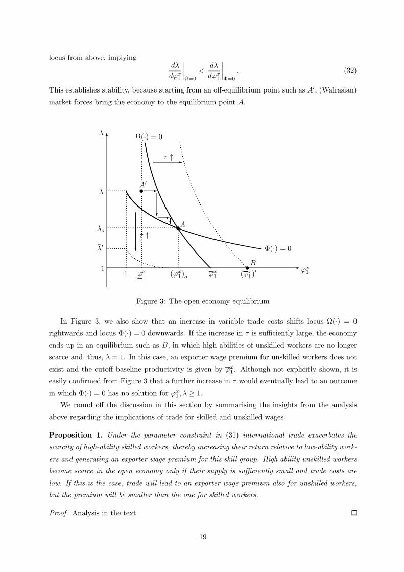
locus from above, implyingdλ

dϕx1

∣∣∣∣Ω=0

<dλ

dϕx1

∣∣∣∣Φ=0

. (32)

This establishes stability, because starting from an off-equilibrium point such as A′, (Walrasian)

market forces bring the economy to the equilibrium point A.

ϕx1

λ

1

λ

1

λ′

!A

(ϕx1)o

λo

!

(ϕx1)

′

B

ϕx1ϕx

1

τ ↑

τ ↑

!

A′

Ω(·) = 0

Φ(·) = 0

Figure 3: The open economy equilibrium

In Figure 3, we also show that an increase in variable trade costs shifts locus Ω(·) = 0

rightwards and locus Φ(·) = 0 downwards. If the increase in τ is sufficiently large, the economy

ends up in an equilibrium such as B, in which high abilities of unskilled workers are no longer

scarce and, thus, λ = 1. In this case, an exporter wage premium for unskilled workers does not

exist and the cutoff baseline productivity is given by ϕx1 . Although not explicitly shown, it is

easily confirmed from Figure 3 that a further increase in τ would eventually lead to an outcome

in which Φ(·) = 0 has no solution for ϕx1 ,λ ≥ 1.

We round off the discussion in this section by summarising the insights from the analysis

above regarding the implications of trade for skilled and unskilled wages.

Proposition 1. Under the parameter constraint in (31) international trade exacerbates the

scarcity of high-ability skilled workers, thereby increasing their return relative to low-ability work-

ers and generating an exporter wage premium for this skill group. High ability unskilled workers

become scarce in the open economy only if their supply is sufficiently small and trade costs are

low. If this is the case, trade will lead to an exporter wage premium also for unskilled workers,

but the premium will be smaller than the one for skilled workers.

Proof. Analysis in the text.

19

The wage effects in Proposition 1 are instrumental for the effects of trade on the economy-wide

inequality level, which are studied in detail in the next section.

4 Trade and income inequality

To measure income inequality we use the Theil index, which for the distribution of individual

labour income w over the interval [w,w] can be computed as

T =

∫ w

w

w

µwln

w

µwdF (w),

where µw is average income, and F (w) is the cumulative distribution function of w. A higher

value of T is associated with higher inequality, and the Theil index has a minimum value of

zero, if income is equally distributed among all workers. A nice feature of the Theil index is

its decomposability, which allows us to split the economy-wide inequality into inequality within

the groups of skilled and unskilled workers, measured by indices Ts and Tu, respectively, and

inequality between the two subgroups, measured by index Tb (see Shorrocks, 1980). For our

model, we can write the economy-wide Theil index as

T = νTs + (1− ν)Tu + Tb,

with

Tb ≡ ν ln

((Lu + Ls)ν

Ls

)+ (1− ν) ln

((Lu + Ls)(1− ν)

Lu

).

Parameters ν and 1−ν measure the income shares of skilled and unskilled workers, respectively,

which due to the Cobb-Douglas technology in Eq. (2) are constant. This implies that access to

exporting has an impact on inequality only through its effect on the Theil sub-indices Ts and

Tu. These subindices are given by

Tu =Lu

Wu

∫ ∞

1wu(β) ln

[Luwu(β)

Wu

]dU(β) (33)

and

Ts =Ls

Ws

∫ ∞

1ws(α) ln

[Ls

Wsws(α)

]dS(α) (34)

Based on the Theil index, trade has the following distributional effects:

Proposition 2. Trade increases the income inequality of skilled workers. The income inequality

of unskilled workers remains unaffected, if there is pooling of unskilled workers over all firms,

whereas it increases in response to trade, if there is pooling of unskilled workers over subsets of

firms. In both cases, the economy-wide inequality is higher in the open than the closed economy.

Proof. See the Appendix.

20

With a pooling of unskilled workers over all firms, the wage profile of unskilled workers is

pinned down by the ability of these workers. As a consequence, the Theil index measuring

the inequality among unskilled workers is unaffected by trade and given by its autarky level:

Tu = Γ − 1 − lnΓ. In this case, we can focus on Ts when studying the consequences of trade

on income inequality. As formally shown in the Appendix, Ts is always larger in the open than

in the closed economy, where Ts = sΘ/g − 1 − ln[sΘ/g]. This is because trade renders skilled

workers with high abilities a scarce resource in our model, which generates an exporter wage

premium and augments income inequality within this skill group. With a pooling of unskilled

workers over subsets of firms, high-ability workers of both skill types become a scarce resource

in the open economy, leading to a wage premium of skilled and unskilled workers employed by

exporting firms. The existence of exporter wage premia gives rise to higher inequality within the

sub-groups of skilled and unskilled workers, adding up to higher economy-wide income inequality.

We complete the discussion in this section by noting that despite a steeper wage profile for

skilled than unskilled workers, it is not clear a priori in our model that Ts > Tu. The reason

is that the Theil index weighs individual wages (relative to the mean) by the relative frequency

of workers receiving this wage. Hence, the scarcity of high abilities among skilled workers,

which is responsible for larger wage differences among skilled than unskilled workers in the first

place, leads to lower weights of high wages in the skilled compared to the unskilled population

of workers, thereby counteracting the direct impact of higher wage differences on skill-specific

Theil indices.

5 Empirical analysis

In this section, we empirically implement the theoretical model outlined above to estimate the

key parameters step by step. For this purpose, we use detailed information on German firms

from the linked employer-employee dataset (LIAB), provided by the Institute for Employment

Research (IAB).13 This dataset matches representative firm-level survey information from the

IAB establishment panel, which is drawn from a stratified sample of establishments with the

stratum being defined over 16 (manufacturing and service) industries, 10 categories of estab-

lishment size, and 16 German states.14 The survey is conducted by Infratest Sozialforschung

on behalf of the IAB, yielding a high response rate of about 80 percent. The dataset includes

important firm characteristics such as the export status as well as total, domestic, and foreign

sales.

LIAB matches the establishment data with individual information on workers who are em-

ployed full-time in one of the establishments in this sample as of 30 June in the respective year.

The individual data comprise information on educational attainment, distinguishing six levels

13Alda et al. (2005) give detailed information on the LIAB dataset, which is confidential but not exclusive, i.e.,it is available for non-commercial research by visiting the research data centre of the German Federal EmploymentAgency at the IAB in Nuremberg, Germany (see also http://fdz.iab.de/en.aspx).

14We use the terms firm and establishment synonymously in this section.

21

of education by the highest degree attained by a worker: 1) lower secondary school, interme-

diate school leaving certificate or less and no vocational training; 2) lower secondary school,

intermediate school leaving certificate or less and vocational training; 3) high-school degree and

no vocational training; 4) high-school degree and vocational training; 5) college degree; and 6)

university degree. We classify individuals from the first education group as unskilled and indi-

viduals with a degree from a college or university as skilled workers (see Sudekum, 2008). With

regard to the three remaining groups, we follow Klein et al. (2013) and use information on the

employment status of a worker to classify her as either skilled (if employed as a white-collar

worker) or unskilled (if employed as a blue-collar worker).15 Our sample covers the years 1996

to 2008, which is the time period before the Subprime Crisis. For this period, we have reli-

able information on establishments all over Germany. Since our model is not informative about

adjustment processes, we do not use the time dimension of the data and instead work with a

cross-section of averages by firm.

We drop all establishments that lack sales or employment information. We also drop estab-

lishments featuring a value added of less than 10 percent of their sales, because some estab-

lishments in the data record negative or other implausible values of value added. This gives

a sample of 22,149 establishments, with 7,024 of these establishments (≈ 31.71 percent) being

active in the export market.

Descriptive statistics of the establishments are summarised in Table 1. As shown in the

table, the average firm in our dataset employs 90.42 workers, with 40.31 percent of its workforce

being skilled according to the adopted definition of this group. Not all firms in the data employ

both skilled and unskilled workers. The skill premium on wages amounts to 28.81 percent. The

wages reported in Table 1 are computed using firm-level averages for the respective skill groups

per annum. The sales level of the average firm in the sample is 26 million Euro. There is a

substantial heterogeneity in firm size, with sales varying between 5.12 thousand and 19.60 billion

Euro, and the workforce varying between 0.04 and 43,225.16 employees.16

The descriptive statistics in Table 1 confirm the insight from previous studies that exporters

are significantly larger than non-exporters, supporting a selection of the best firms into export-

ing (cf. Bernard and Jensen, 1995; Bernard et al., 2012). On average, exporters have 127.31

percent higher sales and employ 116.79 percent more workers than the average (exporting or

non-exporting) firm in the data. At the same time, exporters in the data display a lower skill-

intensity than the average firm. This is in contrast to evidence for Chilean establishments

reported by Harrigan and Reshef (2015). However, it is well in line with our theoretical model,

which explains a low skill intensity of exporters by the scarcity of high-ability skilled workers.

Finally, the descriptives in Table 1 show that the skill premium paid by German exporters is

15In a robustness analysis below, we consider alternative definitions of the groups of skilled and unskilledworkers. Since wages are right-censored, we follow the literature and impute wages for the best-paid employeesin our dataset (see, for instance, Schafer, 1997; Schank et al., 2007). Details on this imputation are available onrequest.

16Fractional values for the number of workers are the result of computing full-year equivalents of the numberof days employed and of averaging establishment information over the covered years.

22

Table 1: Descriptive statistics

Obs. Mean Std. Dev. Min. Max.

– All firms –Nr. of employees 22,149 90.42 465.46 0.04 43,225.16Nr. of unskilled 22,149 53.97 293.36 0.00 25,968.37Nr. of skilled 22,149 36.45 196.98 0.00 17,256.80Wages unskilled 18,062 24,550.78 8,205.45 7,821.95 82,754.99Wages skilled 18,679 31,640.59 12,220.96 7,796.40 95,512.98Sales (in 1,000) 22,149 26,000 215,000 5.12 19,600,000

– Exporters –Nr. of employees 7,024 196.02 780.92 0.33 43,225.16Nr. of unskilled 7,024 123.03 493.54 0.00 25,968.37Nr. of skilled 7,024 72.99 323.63 0.00 17,256.80Wages unskilled 6,221 27,555.06 7,915.31 8,538.78 72,693.95Wages skilled 6,674 37,670.19 11,470.78 7,843.38 95,512.98Sales (in 1,000) 7,024 59,100 363,000 9,742.79 19,600,000

Notes: Figures in this table are based on averages at the firm-level over 1996 to 2008. Wagesand sales levels are in real Euro values (base year 2000).

7.83 percentage points (or 27.12 percent) higher than the skill premium paid by the average Ger-

man firm. This provides further support for our theoretical argument that exporting increases

particularly the scarcity of skilled workers with high abilities.

5.1 Estimation strategy and results

For the fully-fledged quantitative model, we need to estimate seven parameters, namely

ν,σ, g, s, u, η, τ. It is shown in the following that ν, σ, and τ as well as the composite parame-

ters ∆/g and Φ/g can be estimated directly from firm-level information, using OLS. Combining

the estimates of the two composite parameters allows us to recover estimates for g and s as

functions of η. Parameters u and η cannot be estimated from firm level information with-

out knowing the realization of λ ≥ 1. Therefore, we use information on unskilled wages in a

grid-search routine to estimate parameters u and η in consideration of the general equilibrium

constraints imposed by our model. Since the estimation results for u and η do not influence the

other parameter estimates, we can conduct our estimation in two steps.17

17A two-stage estimation procedure similar to ours, with linear regressions in the first stage and GMM inthe second stage, has recently been used by Antras et al. (2017). Also related, Cosar et al. (2016) set severalparameters in accordance to earlier empirical studies and then estimate the remaining parameters using GMM.

23

Step one: OLS estimation of the parameters ν,σ, τ,∆/g,Φ/g

We first estimate the three parameters ν, σ and τ . Parameter ν measures the cost share of skilled

workers in the total wage bill of a firm. We can estimate ν as an average from a regression

ws,vls,vws,vls,v + wu,vlu,v

= ν + errorv. (35)

where v is used as a firm index, and subscripts u and s refer to skilled and unskilled workers.

This yields an estimate of ν = 0.466 with a standard error of 0.003. This estimate is slightly

higher than the skilled labour shares for Mexico reported by Feenstra and Hanson (1997), which

range between 0.37 and 0.41. In contrast to them, we do not distinguish skilled and unskilled

workers by their employment as non-production and production workers, but instead use the

level of educational attainment to distinguish between skill groups.

We estimate σ from the ratio of firm-specific total sales, rv, and operating profits (defined

as value-added net of wage bill), ψv, from a regression of the form

rvψv

= σ + errorv, (36)

Using this procedure, we obtain an estimate of σ = 8.261 with a standard error of 2.933. This

estimate of σ is somewhat higher than the average estimate reported by Broda and Weinstein

(2006), which amounts to 6.5. However, σ lies within the range of parameter estimates typically

found on the basis of gravity equations (cf. Anderson and van Wincoop, 2004, for an overview).

The parameter τ can be estimated according to

rxvrdv

= t0 + errorv (37)

where rdv and rxv are the domestic and foreign sales of an exporting firm, respectively, and

t0 ≡ τ1−σ is a constant. Under the present assumptions, we obtain an estimate of t0 = 0.732

with a standard error of 0.034. In view of the σ-estimate reported above, this corresponds to an

average iceberg-transport-cost parameter of τ = 1.044. This estimate is lower than the trade-

cost estimates typically obtained from gravity equations. For instance, Novy (2013) reports a

τ -estimate for Germany in 2000 of 1.69, whereas Milner and McGowan (2013) estimate τ -levels

for Germany that range from 1.39 to 1.53 between 1996 and 2004.18 However, one should keep

in mind that when relying on the textbook gravity model in a model with heterogeneous firms,

the estimated trade costs comprise both fixed and variable barriers to international trade, and,

hence, it is not surprising that our estimate for τ is lower than the overall trade-cost estimates

from gravity models.19

18We would like to thank Chris Milner for providing country-specific estimates of τ .19We cannot rule out that our assumption of symmetric countries leads us to underestimate the size of the

export market, thereby leading to a downward bias in the estimate of the iceberg-trade-cost parameter. One wayto avoid this potential downward bias in the estimation of τ would be to follow Egger et al. (2013) in formulating amodel with potentially asymmetric countries. However, since our dataset has no information about the destination

24

We now turn to the estimation of composite parameters ∆/g and Φ/g. For this purpose, we

adopt an idea outlined by Arkolakis (2010): With Pareto-distributed productivities and CES

demand, if relative firm-level revenues are a monotonic function of these firms’ productivities

(a feature that our model has, along with most other models building on Melitz, 2003), the

link of a firm’s revenue to its percentile position p in the revenue distribution is informative

about the shape parameter of the underlying Pareto productivity distribution. In our model

with firm-specific skilled wages, an analogous argument holds for the link between the skilled

wage paid by a firm and its percentile position p in the wage distribution.

Since both the revenue distribution and skilled wage distribution across firms are distributed

Pareto in their upper tails, i.e., for all lower truncations ϕ > ϕx2 , with shape parameters

(σ − 1)∆/g and Φ/g, respectively, we can therefore learn about these composite parameters

from linking revenues and skilled wages of exporters with baseline productivity ϕ > ϕ to their

percentile positions in the revenue and skilled wage distribution. Denoting by ϕp the baseline

productivity at percentile p, we can write ϕp/ϕ = (1− Prp/100)−1/g , where Prp ∈ 1, ..., 99 is

the percentile position of a firm with baseline productivity ϕp in the productivity distribution

of exporters with ϕ > ϕ, and rankp ≡ 1 − Prp/100 is the respective firm’s rank in this distri-

bution.20 Denoting by rp and wps average revenues and average skilled wages of firms that are

more productive than firm p, we can derive the following two regression equations:

ln rp = α0 + α1 ln rankp + errorp, (38)

ln wps = β0 + β1 ln rankp + errorp (39)

where α0 and β0 are constants and α1 ≡ −(σ − 1)∆/g and β1 ≡ −Φ/g are functions of the

vector of model parameters x ≡ (ν,σ, s, g, η).21

Except for the requirement that firms considered for the estimation of α1 and β1 must have

a productivity of ϕ > ϕx2 , there is no further constraint confining the choice of ϕ. In the absence

of a strong prior, we estimate Eq. (38) for different realizations of ϕ, which is linked to χ, the

share of exporters with a productivity greater than ϕ, by χ ≡ (ϕ)−g. The different realizations

of ϕ are generated by ordering exporters by their revenues, dividing them into subgroups of

100 producers, and then estimating Eq. (38) for different combinations of these subgroups. In

particular, we estimate parameter α1 for the 100 largest exporters, add the next 100 exporters,

re-estimate parameter α1, and continue this process until the set of subgroups of exporters

of exports, we would not be able to disentangle relative market size from the trade-cost parameter itself withoutadding a new, arbitrary identification assumption. For this reason, and also because the estimation of trade costsis not the main focus of this analysis, we stick to the more parsimonious model variant with symmetric countriesand discuss the aptitude of the model to capture important features of the data below.

20Since observed ranks of firms in the revenue and skilled wage distribution are positively but not perfectlycorrelated, we associate rankp with a firm’s rank in the revenue distribution and therefore approximate theproductivity distribution by the observed distribution of revenues in our dataset.

21Instead of using averages as left-hand side variables, we could simply link each exporter’s revenue and skilledwage to its rank in the respective distribution in order to estimate α1 and β1. However, working with averageshelps guarding against mis-measurement of revenues and wages at the firm level and thus gives more reliableresults.

25

is exhausted. Since our dataset comprises 7,024 exporters, this process gives us 70 different

α1-estimates, which vary over the interval (−0.815,−0.608).

To select a specific parameter estimate, we use the general-equilibrium relationship implied

by the model, according to which total revenues of all exporters, Rx, are linked to total revenues

of exporters with ϕ > ϕ, Rx, by

Rx

Rx= 1 +

(χ

χ− 1

)1

Θ. (40)

Since Rx, Rx, χ, and χ are all observable, we can use Eq. (40) to compute 70 values of Θ,

based on the same subgroups of exporters used earlier for estimating Eq. (38). Accounting for

α1 = 1/Θ − 1 this implies 70 different values for α1. All thus computed values for α1 lie below

the interval of estimated values for α1 from Eq. (38). The largest computed α1 in Eq. (40) –

i.e. the one closest to the interval (−0.815,−0.608) – is generated by χ = 0.05, and hence we

pick the α1-estimate from Eq. (38) that is based on the subgroup of largest exporters that make

up 5 percent of the total firm population. The corresponding estimate is α1 = −0.693 with a

standard error of 0.002.22

This estimate of α1 is close to the Pareto shape parameter reported by Arkolakis (2010) for

foreign sales of French exporters, which amounts to −0.67 when considering uniform fixed costs

and to −0.61 when allowing for fixed costs to be firm-specific. For χ = 0.050, we estimate a

shape parameter of the skilled wage distribution of β1 = −0.047 with a standard error of 0.001.

The parameter estimates for β1 lie in the interval (−0.085,−0.035), which suggests that the

estimate of β1 is not too sensitive to the specific choice of χ.

With the parameter estimates α1 and β1 at hand, we can in a next step use the definitions of

∆ and Φ to solve for estimates of the shape parameters of the baseline productivity distribution,

g, and of the ability distribution of skilled workers, s:

g = −[ν + (1− ν)η](σ − 1)

α1 + ν(σ − 1)β1= 3.975 + 4.546η, (41)

s = −[ν + (1− ν)η](σ − 1)[1 − β1 + α1]

α1 + ν(σ − 1)β1= 1.409 + 1.612η. (42)

The positive impact of η on g and s is intuitive. All other things equal, a larger parameter η

increases the marginal cost differential of two firms resulting from a differential in their baseline

productivities, according to Eq. (7). However, this increase in the marginal cost gap is only

compatible with a given revenue profile over percentiles and thus a given estimate α1, if it is

compensated by a lower relative frequency of high productivity producers and thus a lower

(higher) average productivity in high (low) percentiles of the revenue distribution of exporters.

The reasoning behind the positive relationship of η and s is similar. A larger η allows productivity

differences to exert a larger impact on relative skilled wages (because higher wages become a

22We have checked that χ < (ϕx2)

−g holds for the estimated values of ϕx2 and g, as required by the model.

26

less important cost factor for firms). However, this is compatible with a given skilled wage

profile over percentiles and thus a given estimate of β1 only, if the higher skilled wage gap is

compensated by a lower relative frequency of skilled workers with high abilities. From Eqs. (41)

and (42) we can also infer that s/g = 1− β1 + α1 = 0.355 is independent of η.

One could alternatively formulate the least-squares problems to estimate the parameters

ν, σ, t0, α0,α1, and β0,β1 in terms of a generalised-method-of-moments (GMM)

approach either separately for each parameter type or for all parameters jointly. When allowing

for heteroskedasticity, the GMM estimator is fully equivalent to OLS for each equation as above

(see Greene, 2003, p. 221).

Step two: Estimation of the two remaining parameters η and u

Together with the parameter restrictions from the model, the estimates from above confine the

parameter space of possible combinations of η and u. To see this, note first that condition

s > g + 1− ησ is equivalent to the constraint

η >α1

α1 + β1(σ − 1)≡ η = 0.669. (43)

Furthermore, combining the conditions u < g+1−ησ and u+η−1 > 0 establishes 1−η < g+1−ησ

and, thus, η < η, with

η ≡

⎧⎨

⎩− ν

1−ν+α1+ν(σ−1)β1≡ η0 if η0 ∈ (0, 1)

1 otherwise. (44)

For the parameter estimates from above, we have η0 < 0. This establishes (0.669, 1) as the

relevant domain of η. For parameter u, the relevant domain is confined by the conditions

u + η − 1 > 0 and u < g + 1 − ησ, and this domain is not empty, if η < η. With our

parametrisation, we then have u ∈ (1− η, 4.975 − 3.715η).

To select a unique (η, u)-tuple from the possible parameter space, we conduct the following

grid-search procedure. We first divide the interval [η + 10−7, 1 − 10−7] into 100 symmetric

subintervals and then pick the bounds of these subintervals as possible parametrisations of η.

This gives 101 η-values. For all of these η-values, we then specify a u-interval [1− η+10−7, g+

1−ησ−10−7], divide this interval into 100 subintervals, and choose their boundaries as possible

parametrisations of u. This gives 101 u-values for each η parameter. Altogether, there are then

10,201 candidate (η, u)-tuples that are supported by our model. For all these parameter tuples,

we solve for ϕx1 and λ as described in the theory section, and then compute Theil subindices Tu

and Tw = T −Tb as measures of wage inequality for unskilled workers and the within component

of the overall wage inequality of skilled and unskilled workers.

27

Using the definitions

tu(wu) ≡Luwu

Wuln

Luwu

Wu, t(w) ≡

(Lu + Ls)w

Wu +Wsln

(Lu + Ls)w

Wu +Ws, (45)

we can express the two Theil subindices as functions of tu(wu) and t(w) over the pool of unskilled

workers and the pool of all workers, respectively:

Tu =

∫ wu

wu

tu(wu)dFu(wu), Tw =

∫ w

wt(w)dF (w), (46)

where dFu(wu) is the relative frequency of an unskilled wage of wu in the interval (wu, wu), and

dF (w) is the relative frequency of any (skilled or unskilled) wage w in the interval (w,w). The

Theil subindices Tu and Tw can therefore be interpreted as two data moments that are based on

individual wage observations, and we can use them as inputs for a GMM estimation of η and u

based on the aforementioned grid.23

Whereas targeting two data moments would be sufficient in principle for estimating the two

remaining parameters u and η, we face the problem that Tu and Tw are collinear in our model if

λ = 1. This implies that our econometric model would be underidentified if λ = 1, and, hence,

we would not be able to determine a unique combination of η and u in this case. To overcome

this problem, we target the average wage of unskilled workers with an ability higher than ϕx2 ,

denoted wxu, relative to the average wage of all unskilled workers, Wu/Lu,

Luwxu

Wu=

(ϕx2)

1−ηλν(u+η/ν−s)

1 + (ϕu1 )

u+η−1ωu, (47)

as an additional data moment. With the solution for the general equilibrium at hand, we can

compute theory-consistent measures of Luwxu/Wu for all (η, u)-combinations. Crucially, if λ = 1

(and, thus, ωu = 0), Eq. (47) reduces to Luwxu/Wu = (ϕx

2)1−η, and, hence, only depends on η

but not on u. This implies that Luwxu/Wu and Tu are not collinear, if λ = 1. Finally, we can

express Luwxu/Wu as the (conditional) mean of observables:

Luwxu

Wu=

∫ wu

wxu

Luwu

WudF x

u (wu), (48)

where wxu is the lower bound of wages received by unskilled workers with abilities β ≥ ϕx

2 and

dF xu (w

xu) is the conditional relative frequency of unskilled wages over interval (wx

u/wu), i.e.,

dF xu (wu) = dFu(wu)/[1− Fu(wx

u)], with 1− Fu(wxu) = (φx2)

−u.

Taking stock, we have identified three moment conditions in two parameters, which we denote

by mu(η, u) for targeting Tu, mw(η, u) for targeting Tw, and mr(η, u) for targeting the average

23To be consistent with the previous estimations and with the results of the model, when constructing t(w) weimpose the restriction that firms pay the same (average) wage to all their skilled workers.

28

wage of skilled workers with β > ϕx2 . We select the preferred (η, u)-tuple as the solution to

argmin(η,u)

m′Ψm, (49)

where m is a 3x1 vector of the moment conditions and Ψ is a 3x3 positive semi-definite moments

weighting matrix. To give more precisely measured moments a higher weight in the estimation,

we weigh the moment conditions by the inverse variance of the data underlying the construction

of the respective averages and estimate parameter values of η = 0.987 and u = 0.052 with

standard errors of 0.001 and 0.005, respectively. These parameter estimates represent interior

solutions, i.e. neither η nor u lie at their interval bounds, and they support an outcome with

λ = 1 and, thus, a pooling of unskilled workers over all firms.24

To get an intuition for the estimates of η and u, one should bear in mind that for λ = 1, η is

disciplined by the third moment condition, which links average wages from an upper tail of the

ability distribution of unskilled workers in the model to the average wage of unskilled workers

employed by high productivity firms in the data. Since the ability distribution in the model

does not have an upper bound, a good fit of the model with this specific moment requires that

the elasticity of the wage profile of unskilled workers is sufficiently small, so that the impact

of ability differences on wages is not too high.25 The low estimate of u is then the result of

bringing a high η and thus a relatively flat wage profile in accordance with the sizable Theil

index of unskilled workers’ incomes observed in the data. The parameter estimate of η allows us

to compute implied estimates of the shape parameters of the productivity distribution and the

ability distribution of skilled workers, which we estimate at g = 8.461 and s = 3.000, respectively.

We complete the discussion in this section by summarising the point estimates for our pa-

rameters and the main composites of these parameters in Table 2. To account for remaining

interdependencies of the parameter estimates, which are not adequately addressed by OLS, we

have computed standard errors from 50 bootstrap samples of the data, which differ slightly

from the estimated standard errors in the text. We report the bootstrapped standard errors in

parentheses.

5.2 Model fit

With the parameter estimates derived in the previous section, we can quantify economy-wide

inequality and its components, and contrast the respective results with the empirical patterns

in our dataset. Table 3 reports the computed and observed measures of inequality (with boot-

strapped standard errors in parentheses). Our model underestimates the various forms of wage

24The weighting matrix only matters if there are more moment conditions than parameters to estimate, whichis the case in our application if λ > 1. Hence, with λ = 1, our parameter estimates do not change when givingequal weight to all moment conditions, or when using the inverse of the estimated variance-covariance matrix ofthe moment conditions for specifying Ψ, as recommended by Hansen (1982).

25Note that in our model 1 − η captures the effect of abilities on effective firm productivity conditional on

abilities being higher than the minimum viable level. Therefore our high estimate for η is compatible with theunderlying model assumption that abilities are important for determining this productivity.

29

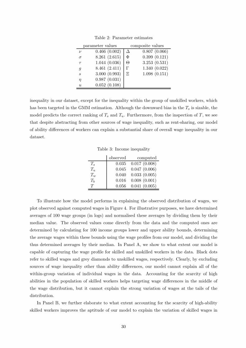
Table 2: Parameter estimates

parameter values composite valuesν 0.466 (0.002) ∆ 0.807 (0.066)σ 8.261 (2.615) Φ 0.399 (0.121)τ 1.044 (0.036) Θ 3.253 (0.531)g 8.461 (2.411) Γ 1.340 (0.022)s 3.000 (0.993) Ξ 1.098 (0.151)η 0.987 (0.031)u 0.052 (0.108)

inequality in our dataset, except for the inequality within the group of unskilled workers, which

has been targeted in the GMM estimation. Although the downward bias in the Ts is sizable, the

model predicts the correct ranking of Ts and Tu. Furthermore, from the inspection of T , we see

that despite abstracting from other sources of wage inequality, such as rent-sharing, our model

of ability differences of workers can explain a substantial share of overall wage inequality in our

dataset.

Table 3: Income inequality

observed computedTs 0.035 0.017 (0.008)Tu 0.045 0.047 (0.006)Tw 0.040 0.033 (0.005)Tb 0.016 0.008 (0.001)T 0.056 0.041 (0.005)

To illustrate how the model performs in explaining the observed distribution of wages, we

plot observed against computed wages in Figure 4. For illustrative purposes, we have determined

averages of 100 wage groups (in logs) and normalised these averages by dividing them by their

median value. The observed values come directly from the data and the computed ones are

determined by calculating for 100 income groups lower and upper ability bounds, determining

the average wages within these bounds using the wage profiles from our model, and dividing the

thus determined averages by their median. In Panel A, we show to what extent our model is

capable of capturing the wage profile for skilled and unskilled workers in the data. Black dots

refer to skilled wages and grey diamonds to unskilled wages, respectively. Clearly, by excluding

sources of wage inequality other than ability differences, our model cannot explain all of the

within-group variation of individual wages in the data. Accounting for the scarcity of high

abilities in the population of skilled workers helps targeting wage differences in the middle of

the wage distribution, but it cannot explain the strong variation of wages at the tails of the

distribution.

In Panel B, we further elaborate to what extent accounting for the scarcity of high-ability

skilled workers improves the aptitude of our model to explain the variation of skilled wages in

30

!!"# !"# !"$ !"%

!&"!

!!"'

!"'

!!"# !"# !"$ !"%

!&"!

!!"'

!"'

observed

(normalised

)wag

es

computed (normalised) wages

skilled workers unskilled workers

Panel A: Skilled and Unskilled Wages

observed

(normalised

)wag

es

computed (normalised) wages

separation pooling

Panel B: Separation and Pooling of Skilled Workers

Figure 4: Observed versus computed wages

the data. For this purpose, we contrast the separating equilibrium supported by the data (black

dots) with a pooling equilibrium of skilled workers, featuring an elasticity of the wage profile

that is equal to 1 − η. Relying on our parameter estimates, we see that ignoring the scarcity

of high abilities would lead our model to underestimate the high variation of skilled wages to

a much larger extent than the preferred specification with a separating equilibrium of skilled

workers.

Figure 4 suggests that accounting for the the scarcity of skilled workers with high abilities

improves the fit of the data by our model. We can go one step further and quantify this

improvement by computing the divergence between the observed and computed distribution of

skilled wages. For this purpose, we can rely on an index of divergence introduced by Kullback and

Leibler (1951), which measures the information loss from approximating the true distribution

of wages by the distribution from our model.26 The Kullback-Leibler divergence gives the

expected logarithmic difference between the true probability distribution of variable x, P r(x),

and its theoretical approximation, Pr(x). For discrete distributions it is given by

D(P r||Pr) =∑

x

P r(x)

[ln

(P r(x)

Pr(x)

)], (50)

where P r(x) = 0 whenever Pr(x) = 0. The Kullback-Leibler divergence takes on a value of zero,

if two distributions are identical, and it is larger than zero otherwise. Lower values of D(P r||Pr)

indicate a smaller information loss and thus a better approximation of the true distribution of

x by Pr.

We can now associate xi with a realization of wages in wage group i, and therefore interpret

P r(xi) as the probability that a random draw of a skilled worker from our dataset gives an

observation in wage group i. Since the 100 wage groups are disjoint and of (almost) equal size,

26Mrazova et al. (2016) provide a detailed discussion about the properties of the Kullback-Leibler index and itsrelationship to Shannon’s (1948) entropy.

31

we have P r(xi) ≈ 0.01 for all i ∈ 1, ..., 100.27 For constructing the values of Pr(xi), we

consider observed lower and upper bounds of skilled wages for each wage group and construct

ability bounds from the wage profile of skilled workers in our model. The thus computed ability

bounds are then used to determine Pr(xi) =∫ αi

αiα−sdS(α). Using P r(xi) and Pr(xi) in Eq.

(50) gives

Ds(P r||Pr) = 0.001 and Dp(P r||Pr) = 2.300 (51)

for the baseline specification with a separating equilibrium for skilled workers and a counterfac-

tual situation with a pooling equilibrium of skilled workers, respectively. The sizable difference

between the two divergence measures confirms our conjecture from Figure 4 that accounting

for the scarcity of high-ability skilled workers improves the fit of our model with the observed

distribution of skilled wages considerably.

6 The exporter wage premium and its effect on inequality

When it comes to quantifying the exporter wage premium, the structural approach employed in

this paper, unlike previous studies, allows us to compute skill-specific premia. The parameter

estimates derived above imply u + η/ν − s < 0, which means that there is no exporter wage

premium for unskilled workers. By contrast, the exporter premium for skilled workers is large and

amounts to 12.137 percent. Weighting the skill-specific wage premia by the share of skilled and

unskilled workers employed in exporting firms, we arrive at an average exporter wage premium of

4.896 percent. This average is at the lower bound of results from previous empirical work, which

reports estimates that vary between four and eighteen percent (cf. Bernard and Jensen, 1999;

Mayer and Ottaviano, 2008; Frias et al., 2009; Egger et al., 2013; Hauptmann and Schmerer,

2013), when not distinguishing between skilled and unskilled workers. Using the same dataset

as we do, Klein et al. (2013) estimate an average exporter wage premium for Germany of 4.4

percent in a reduced-form approach.28

To provide a better understanding of how the existence of an exporter wage premium affects

economy-wide wage inequality in our model, we can quantify the impact of trade on wage

inequality in Germany by contrasting the Theil indices for the observed exposure to trade with

the respective indices in the counterfactual situation without any trade. Moving the German

economy to autarky means eliminating the exporter wage premium by design. Since exporters

do not pay a wage premium to their unskilled workforce, this comparative static exercise only

affects the wage distribution of skilled workers, making it more equal. Specifically, the Theil

index measuring the wage distribution of skilled wages, Ts, declines by 35.975 percent, whereas

27Due to indivisibilities, small deviations from !Pr(xi) = 0.01 are possible.28Schank et al. (2007) report much smaller exporter wage premia for Germany. According to their findings,

plants with an export to sales ratio of 60 percent pay 1.8 percent higher wages to unskilled and 0.9 percent higherwages to skilled workers than otherwise identical non-exporting plants.

32

the overall wage inequality, as measured by the Theil index T , falls by 6.783 percent.29

As an alternative counterfactual exercise, we consider the case of abolishing all variable

trade costs, while leaving the fixed export costs constant. At the observed exposure to trade,

χ = 0.317, we can compute an estimate of fx/fe by employing the parameter estimates in Eq.

(27). This establishes !fx/fe = 0.414. Equipped with this fixed cost ratio, we can then apply

the implicit function in Eq. (27) to compute the share of exporting firms if τ falls to unity. This

gives χ = 0.466 and indicates that eliminating iceberg trade costs has a considerable effect on

the share of exporting firms. Regarding the effect on inequality, there are now two potentially

counteracting effects: An increase in the exporter wage premium, which increases inequality,

and an increase in the share of the skilled worker population being paid this premium. The

latter effect is non-monotonic, becoming negative if χ is sufficiently large. In line with this

reasoning, the distributional effects of our counterfactual exercise are small. The exporter wage

premium for skilled workers would increase by 2.720 percent and would be counteracted and

dominated by an increase in the share of skilled workers employed by exporters, so that wage

inequality within the group of skilled workers would be reduced if variable trade costs fell to

zero. Specifically, we find that the Theil index of skilled workers falls by 1.729 percent, whereas

the Theil index for all workers falls by 0.326 percent.

7 Robustness analysis

In this section, we analyse the robustness of our estimation results regarding the distinction of

skilled and unskilled workers. For this purpose, we consider two alternative definitions of skill

groups: a narrow definition, in which we associate the skilled with those workers who hold a

college or university degree; and a broad definition, in which we classify only workers as unskilled

if their highest degree attained is one of a lower secondary education and if they lack vocational

training. The parameter estimates for these two alternative skill definitions are summarised in

Table 4. To facilitate the discussion, we have added our estimates from the benchmark scenario,

whereas we do not report the estimates for σ, τ , and Θ, as they are independent of the chosen

skill definitions.

From the ν-estimates in Table 4, we can conclude that the considered changes in the skill def-

initions have large effects on the income shares of the two skill groups. However, the effects on

the other parameter estimates are rather small and, relying on the bootstrapped standard errors

from the benchmark scenario, the differences in most cases are statistically insignificant. Fur-

thermore, where a direct economic interpretation of the parameters is applicable, the observed

changes in the point estimates seem to be well in line with standard economic reasoning.

For instance, classifying as skilled only those workers who hold a college or university degree

makes abilities of skilled workers more similar, and therefore leads to a higher estimate of s,

29With constant expenditure shares due to the Cobb-Douglas technology and full employment of both skilltypes, there are no effects on the relative return of skilled to unskilled workers on average, leaving the betweencomponent of the Theil index, Tb, unaffected.

33

Table 4: Parameter estimates for alternative skill definitions

parameter benchmark narrow skill broad skillν 0.466 0.106 0.841g 8.461 9.914 7.438s 3.000 3.480 2.632η 0.987 0.991 0.997u 0.052 0.037 0.013∆ 0.807 0.946 0.709Φ 0.399 0.432 0.345Γ 1.340 1.346 1.326Ξ 1.098 0.630 1.241

whose value approaches infinity in the limiting case of fully symmetric agents. Of course, one

would also expect a higher elasticity of the skilled wage schedule when skilled workers with high

abilities are a scarcer resource, i.e., when s is higher. This reasoning is in line with a higher

estimate of Φ for the scenario with a narrow skill definition. Finally, since the markup per

efficiency unit paid to skilled workers with higher abilities lowers the effect that differences in

the baseline productivity exert on marginal costs, one would expect that the elasticity of firm-

level marginal costs with respect to productivity declines, when skilled workers become a less

important cost factor as fewer of them are employed by firms. This conjecture is confirmed by

a higher estimate of ∆ when considering the narrow skill definition.

Choosing alternative definitions of skill groups also affects the observed measures of wage

inequality. This can be seen from Table 5, where we report the various Theil indices discussed

above for the benchmark scenario as well as the two alternative skill definitions. As expected,

the broader the definition of a skill group is, the larger is the wage inequality in this group.

Interestingly, we observe for both the narrower as well as the broader skill definition that the

share of wage inequality attributed to the within component increases in the data. Our model is

not overly successful in capturing the between-component of the Theil index, but it does a fairly

good job in predicting wage inequality within the subgroups of skilled and unskilled workers, in

particular when considering the narrow skill definition.

Table 5: Theil indices for alternative skill definitions

benchmark narrow skill def. broad skill def.observed computed observed computed observed computed

Ts 0.035 0.017 0.029 0.028 0.040 0.014Tu 0.045 0.047 0.058 0.049 0.038 0.044Tw 0.040 0.033 0.053 0.047 0.040 0.018Tb 0.016 0.008 0.016 0.001 0.007 0.044T 0.056 0.041 0.069 0.048 0.047 0.063

With the parameter estimates from Table 4 at hand, we can finally compute the exporter

wage premium. For skilled workers this premium amounts to 34.367 percent when considering a

34

narrow skill definition, which is almost three times as high as in the benchmark scenario. Since

u + η/ν − s > 0 holds, the necessary condition for an exporter wage premium for unskilled

workers is met, but we estimate λ < 1, which enforces λ = 1 and thus ωu = 0. The average

exporter wage premium for all skilled and unskilled workers amounts to 4.520 percent for the

narrow skill definition, which is of the same order of magnitude as in the benchmark scenario.

Relying on the broad skill definition, we estimate an exporter wage premium for skilled workers

of 7.244 percent. Whereas u+η/ν−s < 0 does not leave scope for an exporter wage premium of

unskilled workers, the average exporter wage premium for skilled and unskilled workers amounts

to 4.930. This confirms the insight from above that the estimate of the average exporter wage

premium is robust to changes in the definition of skill groups.

8 Conclusion

We have proposed a structural empirical model of an open economy in which the populations of

firms and workers are heterogeneous. Firms hire skilled and unskilled workers for production, and

firms with a higher (innate) baseline productivity require skilled and unskilled workers of higher

ability, leading them to pay higher wages for both types of workers. With more productive firms

selecting into exporting, our model allows for the existence of an exporter wage premium due

to extra demand by exporting firms for high-ability workers that are in fixed supply. Whether

or not an exporter wage premium materialises in our model depends on the supply of and the

demand for workers with high abilities, and, therefore, on the ability distributions of skilled

and unskilled workers as well as on the baseline productivity distribution of firms. With two

types of workers present, we can decompose the exporter wage premium into its skill-specific

components.

We structurally estimate the parameters of the model using the matched employer-employee

dataset LIAB of the Institute for Employment Reserch (IAB), which provides detailed informa-

tion on German firms and workers for the years 1996 to 2008. The dataset provides information

on the educational background of workers as well as their employment as blue- or white-collar

workers. We use this information to find the empirical equivalent of the skilled and unskilled

worker categories in our theoretical model. Using the estimated parameter values, we find an

average exporter wage premium of about 5 percent, which is within the range of values reported

in other studies. But we also find that this average masks a lot of heterogeneity, with export-

ing firms paying no wage premium to their unskilled workers, while the exporter wage premium

for the subgroup of skilled workers is higher than 12 percent. This suggests to us that it is

empirically relevant to dissect the exporter wage premium as we have done in this paper.

Through its effect on the exporter wage premium, trade in the proposed model has consider-

able effects on the economy-wide distribution of income, which is more unequal in the open than

the closed economy. However, the respective effects are not monotonic, implying that traveling

further along the road of trade liberalisation will eventually reduce income inequality, despite

35

an increase in the exporter wage premium. The reason for this is that less productive firms start

exporting, employing workers with lower abilities and thus from lower segments of the wage dis-

tribution. In two extensions, we show that the main insights from our analysis are robust to

quite substantial changes in the definitions of skilled and unskilled workers.

References

Alda, H., S. Bender, and H. Gartner (2005): “The Linked Employer-employee DatasetCreated from the IAB Establishment Panel and the Process-produced Data of the IAB(LIAB),” Schmollers Jahrbuch, 125, 327–336.

Amiti, M. and D. R. Davis (2012): “Trade, Firms, and Wages: Theory and Evidence,” Review

of Economic Studies, 79, 1–36.

Anderson, J. E. and E. van Wincoop (2004): “Trade Costs,” Journal of Economic Litera-

ture, 42, 691–751.

Antras, P., T. Fort, and F. Tintelnot (2017): “The Margins of Global Sourcing: Theoryand Evidence from U.S. Firms,” American Economic Review, forthcoming.

Arkolakis, C. (2010): “Market Penetration Costs and the New Consumers Margin in Inter-national Trade,” Journal of Political Economy, 118, 1151–1199.

Armenter, R. and M. Koren (2015): “Economies of Scale and the Size of Exporters,”Journal of the European Economic Association, 13, 482–511.

Bernard, A. B. and J. B. Jensen (1995): “Exporters, Jobs, and Wages in U.S. Manufactur-ing: 1976-1987,” Brookings Papers on Economic Activity. Microeconomics, 67–119.

——— (1999): “Exceptional Exporter Performance: Cause, Effect, or Both?” Journal of Inter-

national Economics, 47, 1–25.

Bernard, A. B., J. B. Jensen, S. J. Redding, and P. K. Schott (2012): “The Empiricsof Firm Heterogeneity and International Trade,” Annual Review of Economics, 4, 283–313.

Broda, C. and D. E. Weinstein (2006): “Globalization and the Gains from Variety,” Quar-

terly Journal of Economics, 121, 541–585.

Cosar, A. K., N. Guner, and J. Tybout (2016): “Firm Dynamics, Job Turnover, and WageDistributions in an Open Economy.” American Economic Review, 106, 625–663.

Davis, D. R. and J. Harrigan (2011): “Good Jobs, Bad Jobs, and Trade Liberalization,”Journal of International Economics, 84, 26–36.

Egger, H., P. Egger, and U. Kreickemeier (2013): “Trade, Wages, and Profits,” European

Economic Review, 64, 332 – 350.

Egger, H. and U. Kreickemeier (2009): “Firm Heterogeneity And The Labor Market EffectsOf Trade Liberalization,” International Economic Review, 50, 187–216.

——— (2012): “Fairness, Trade, and Inequality,” Journal of International Economics, 86, 184–196.

Feenstra, R. C. and G. H. Hanson (1997): “Foreign Direct Investment and Relative Wages:Evidence from Mexico’s Maquiladoras,” Journal of International Economics, 42, 371–393.

36

Frias, J. A., D. S. Kaplan, and E. Verhoogen (2009): “Exports and Wage Premia:Evidence from Mexican Employer-Employee Data,” unpublished manuscript.

Ghironi, F. and M. J. Melitz (2005): “International Trade and Macroeconomic Dynamicswith Heterogeneous Firms,” Quarterly Journal of Economics, 120, 865–915.

Greene, W. (2003): Econometric Analysis, Prentice Hall, New Jersey, 5th ed.

Hansen, L. P. (1982): “Large Sample Properties of Generalized Method of Moments Estima-tors,” Econometrica, 50, 1029–1054.

Harrigan, J. and A. Reshef (2015): “Skill Biased Heterogeneous Firms, Trade Liberalizationand the Skill Premium,” Canadian Journal of Economics, 48, 1024–1066.

Hauptmann, A. and H.-J. Schmerer (2013): “Do Exporters Pay Fair-wage Premiums?”Economics Letters, 121, 179–182.

Helpman, E., O. Itskhoki, and S. Redding (2010): “Inequality and Unemployment in aGlobal Economy,” Econometrica, 78, 1239–1283.

Irrazabal, A., A. Moxnes, and K. H. Ulltveit-Moe (2013): “Heterogeneous Firms orHeterogeneous Workers? Implications for Exporter Premiums and the Gains from Trade,”Review of Economics and Statistics, 95, 839–849.

Klein, M., C. Moser, and D. Urban (2013): “Exporting, Skills and Wage Inequality,”Labour Economics, 25, 76–85.

Kullback, S. and R. A. Leibler (1951): “On Information and Sufficiency,” The Annals of

Mathematical Statistics, 22, 79–86.

Mayer, T. and G. I. Ottaviano (2008): “The Happy Few: The Internationalisation ofEuropean Firms – New Facts based on Firm-level Evidence,” Intereconomics, 44, 149–158.

Melitz, M. J. (2003): “The Impact of Trade on Intra-Industry Reallocations and AggregateIndustry Productivity,” Econometrica, 71, 1695–1725.

Milner, C. and D. McGowan (2013): “Trade Costs and Trade Composition,” Economic

Inquiry, 51, 1886–1902.

Mrazova, M., P. Neary, and M. Parenti (2016): “Sales and Markup Dispersion: Theoryand Empirics,” Unpublished Manuscript.

Novy, D. (2013): “Gravity Redux: Measuring International Trade Costs with Panel Data,”Economic Inquiry, 51, 101–121.

Sampson, T. (2014): “Selection into Trade and Wage Inequality,” American Economic Journal:

Microeconomics, 6, 157–202.

Schafer, J. (1997): Analysis of Incomplete Multivariate Data, Chapman and Hall/CRC.

Schank, T., C. Schnabel, and J. Wagner (2007): “Do Exporters Really Pay Higher Wages?First Evidence from German Linked Employer-Employee Data,” Journal of International

Economics, 72, 52–74.

Shannon, C. E. (1948): “A Mathematical Theory of Communication,” Bell System Technical

Journal, 27, 379–423.

37

Shorrocks, A. F. (1980): “The Class of Additively Decomposable Inequality Measures,”Econometrica, 48, 613–625.

Sudekum, J. (2008): “Convergence of the Skill Composition Across German Regions,” Regional

Science and Urban Economics, 38.

38

A Appendix

A.1 Proof of Lemma 1

To prove Lemma 1, we proceed in two steps. First, we show that with pooling of unskilled workers

over all firms, s ≥ g + 1 − ησ is necessary and sufficient for segmentation of skilled workers by

firms. Second, we show that with segmentation of skilled workers by firms u < g + 1 − ησ is

sufficient for pooling of unskilled workers by firms. Together, the two conditions then establish

Lemma 1.

Let us first consider pooling of unskilled workers over all firms. In this case, wage differences

reflect ability differences, and the wage paid to a worker with ability β are linked to the wage

paid to the least able unskilled worker, with ability βc, who finds employment in the least

productive firm, featuring productivity ϕc, by wu(β) = (β/βc)1−ηwu(βc). Let us further assume

that skilled workers were also just compensated for their ability differences, implying that skilled

wages would be given by ws(α) = (α/αc)1−ηws(αc), with αc = ϕc. In this case, our model would

mimic a textbook Melitz (2003) model with the productivity of firms given by ϕη and, since all

producers pay the same wage per efficiency unit for labour input, marginal costs are inversely

proportional to to this productivity. If firms in such a situation were only employing those

skilled workers that exactly match their productivity threshold, i.e., if α = ϕ would hold for

all ϕ, the assumption of a Cobb-Douglas technology would give rise to ws(v)ls(v) = νc(v)q(v).

Accordingly, firm-level demand for skilled workers could be expressed by ls(v) = (ϕ(v)/ϕc)ησ−1lcs,

where lcs and ϕc refer to the number of skilled workers employed by and the baseline productivity

of the least productive producer, respectively. Suppressing firm index v, total labour demand of

all firms with productivity higher than ϕ would be given by Nlcs[g/(g − ησ + 1)](ϕ/ϕc)ησ−g−1,

where N is the mass of producers. The supply of workers with ability higher than ϕ equals

Lsϕ−s, and labour market clearing at ϕ = ϕc therefore requires Nlcs[g/(g − ησ + 1)] = Lsϕ−sc .

Putting together, we find that under labour market clearing g+1− ησ > s would lead to excess

supply of skilled workers with ability β > ϕc in the knife-edge case, in which firms employ skilled

workers whose ability corresponds to their productivity threshold and pay the same wage per

efficiency unit for either skill group. This would result in firms hiring workers with abilities

above their productivity threshold and thus establish pooling of skilled workers over firms. In

contrast, s > g + 1 − ησ would lead to excess demand of skilled workers in the thus described

knife-edge case and ultimately lead to a separating equilibrium and a skilled wage profile that

is steeper than required for a compensation of ability differences.

Let us now consider segmentation of skilled workers by firms and let us hypothesise that

firms hire only unskilled workers that exactly match their technology requirements, β = ϕ,

paying them a wage of wu(β) = (β/βc)1−ηwu(βc). Using Eqs. (5) and (9) from Section 2.3, we

can write firm-level employment of unskilled workers as lu(ϕ) = (ϕ/ϕc)∆(σ−1)−1+η lu(ϕc). The

demand for unskilled workers of firms with productivity ϕ > ϕ is given by Nlcu[g/(g −∆(σ −

1)− 1 + η)](ϕ/ϕc)∆(σ−1)−g+1−η , whereas supply of unskilled workers with ability higher than ϕ

equals Luϕ−u. With labour market clearing at ϕ = ϕc, we find that there is an excess supply

of unskilled workers in the knife-edge case considered here, if u < g − ∆(σ − 1) + 1 − η. In

39

this case, we have pooling of unskilled workers over all firms, whereas there is segmentation of

unskilled workers over firms if u > g − ∆(σ − 1) + 1 − η. Noting further that ∆ − η ≤ 0 is

established by s ≥ g + 1 − ησ, one can confirm that the parameter constraint in Assumption

1 establishes pooling of unskilled workers if there is segmentation of skilled workers by firms.

Putting together, we can thus conclude that with this parameter constraint the only possible

outcome consistent with labour market clearing is one with segmentation of skilled workers by

firms and pooling of unskilled workers over firms. This completes the proof.

A.2 Wage profiles of skilled and unskilled workers in the open economy

Let us consider the productivity thresholds ϕx1 ,ϕ

x2 as defined in the main text. Then, for

all ϕ ∈ [ϕx1 ,ϕ

x2), exporters and non-exporters coexist, and, hence, it must be true that (1 +

τ1−σ)r(ϕ)/σ − r(ϕ)/σ = fx and thus τ1−σr(ϕ) = σfx. Accounting for r(ϕ) = p(ϕ)q(ϕ) and Eq.

(8) from the closed economy, we obtain the revenue profile for the open economy:

r(ϕ) =

⎧⎪⎪⎪⎪⎪⎪⎨

⎪⎪⎪⎪⎪⎪⎩

ϕ(σ−1)∆r(1) if ϕ < ϕx1

(ϕx1)

(σ−1)∆r(1) if ϕ ∈ [ϕx1 ,ϕ

x2)

ϕ(σ−1)∆(ϕx1

ϕx2

)(σ−1)∆r(1) if ϕ ≥ ϕx

2

(A.1)

Furthermore, the wage profile of skilled workers can be expressed as

ws(ϕ)

ws(1)=

⎧⎪⎪⎪⎪⎪⎪⎨

⎪⎪⎪⎪⎪⎪⎩

ϕ− gΘ+s if ϕ < ϕx

1

ϕ−g+s[1 + τ1−σχ(ϕ)](ϕx1 )

gΘ−1Θ if ϕ ∈ [ϕx

1 ,ϕx2)

ϕ− gΘ+s[1 + τ1−σ]

(ϕx1

ϕx2

)gΘ−1Θ

if ϕ ≥ ϕx2

(A.2)

where we have used Eq. (8) together with [ν + (1 − ν)η]/ν −∆/ν = −g/Θ + s, and χ(ϕ) = 0

if ϕ < ϕx1 to establish the first line in Eq. (A.2). The second line is obtained from our previous

result that r(ϕ) = r(ϕx1) holds for all ϕ ∈ [ϕx

1 ,ϕx2) and the insight that a fraction χ(ϕ) of firms

of productivity ϕ exports over productivity interval [ϕx1 ,ϕ

x2). Skilled labour demand of firms

with productivity ϕ ∈ (ϕx1 ,ϕ

x2 ] is therefore proportional to [1+ τ1−σχ(ϕ)]ws(ϕ), and these firms

exist with density gϕ−g−1, whereas skilled workers with ability α = ϕ exist with density sϕ−s−1.

Equalising supply and demand for all ϕ ∈ [ϕx1 ,ϕ

x2) therefore requires a wage profile over this

productivity subdomain as given by the second line of (A.2). Finally, the third line is derived

in analogy to the first line, accounting for χ(ϕ) = 1 if ϕ ≥ ϕx2 .

To determine the wage profile of unskilled workers in Eq. (17), let us assume that there

exists an interval [ϕu1 ,ϕ

u2 ), such that there is segmentation of unskilled workers by firms over

this productivity interval. Under Assumption 1 and a Cobb-Douglas technology, it is immediate

that ϕu1 ,ϕ

u2 ∈ (ϕx

1 ,ϕx2). From the discussion of the closed economy, it follows that wu(β)/wu(1) =

β1−η holds for all β < ϕu1 , establishing the first line in Eq. (17). With segmentation of skilled

and unskilled workers by firms, the marginal cost of a firm with productivity ϕ ∈ [ϕu1 ,ϕ

u2 ) is

40

given by

c(ϕ) = µwu(ϕ)

ϕ

(ws(ϕ)

wu(ϕ)

)ν

, (A.3)

where β = ϕ and thus wu(β) = wu(ϕ) have been considered. From the assumption of a Cobb-

Douglas technology paired with the requirement that labour markets of skilled and unskilled

workers clear for all ϕ ∈ [ϕu1 ,ϕ

u2 ), we further have

ν

1− ν=

Lssϕ−s−1ws(ϕ)

Luuϕ−u−1wu(ϕ), (A.4)

implying c(ϕ) ∝ wu(ϕ)ϕ−1−ν(u−s). This establishes wu(β)/wu(ϕu1 ) = (ϕ/ϕu

1 )1+ν(u−s) and thus

the second line in Eq. (17). For the third line, we can simply note that wu(β)/wu(ϕu2 ) =

(β/ϕu2 )

1−η holds for all β > ϕu2 , whereas wu(ϕu

2)/wu(1) = (ϕu2/ϕ

u1 )

ν(u+η/ν−s)(ϕu2 )

1−η follows

from above. This completes the formal characterisation of the two wage profiles.

A.3 Derivation of Eq. (18)

Provided that [ϕu1 ,ϕ

u2 ) is not empty, we have to distinguish five productivity domains. The first

one is ϕ < ϕx1 and implies χ(ϕ) = 0. The second one is ϕ ≥ ϕx

2 and establishes χ(ϕ) = 1.

The third productivity domain is given by ϕ ∈ [ϕx1 ,ϕ

u1 ). In this case, we have segmentation of

skilled workers and pooling of unskilled workers, establishing c(ϕ) ∝ ws(ϕ)νϕ−ν−η(1−ν). Since

we know from above that r(ϕ) = r(ϕx1) an thus c(ϕ) = c(ϕx

1) holds for all ϕ ∈ [ϕx1 ,ϕ

x2),

we can solve for ws(ϕ)/ws(ϕx1) = (ϕ/ϕx

1)1+η(1−ν)/ν . Equating the latter with ws(ϕ)/ws(ϕx

1) =

(ϕ/ϕx1 )

−g+s[1+τ1−σχ(ϕ)] from the second line of Eq. (A.2) establishes the second line in Eq. (18).

The fourth segment, we have to consider is one with ϕ ∈ [ϕu1 ,ϕ

u2 ). In this case, we have

segmentation of skilled and unskilled workers by firms and thus c(ϕ) ∝ wu(ϕ)ϕ−1−ν(u−s) (see

above) or, equivalently, c(ϕ) ∝ ws(ϕ)ϕ−1−(1−ν)(s−u). Since we have c(ϕ) = c(ϕu1 ), we can solve

for ws(ϕ)/ws(ϕu1 ) = (ϕ/ϕu

1 )1+(1−ν)(s−u). Accounting for ws(ϕu

1 )/ws(ϕx1) = (ϕu

1/ϕx1)

1+η(1−ν)/ν ,

we obtain

ws(ϕ)

ws(ϕx1)

=

(ϕu1

ϕx1

) ν+η(1−ν)ν

(ϕ

ϕu1

)1+(1−ν)(s−u)

(A.5)

Equating Eq. (A.5) with ws(ϕ)/ws(ϕx1) = (ϕ/ϕx

1 )−g+s[1 + τ1−σχ(ϕ)] and accounting for 1 +

η(1 − ν)/ν + g − s = ∆[1 + ν(σ − 1)]/ν gives the third line in Eq. (18). The fifth productivity

segment corresponds to ϕ ∈ [ϕu2 ,ϕ

x2). In this case, we have c(ϕ) ∝ ws(ϕ)νϕ−ν−η(1−ν) and, in

view of c(ϕ) = c(ϕu2 ): ws(ϕ)/ws(ϕu

2) = (ϕ/ϕu2 )

1+η(1−ν)/ν . Evaluating Eq. (A.5) at ϕ = ϕu2 , we

obtain

ws(ϕ)

ws(ϕx1)

=

(ϕ

ϕx1

) ν+η(1−ν)ν

(ϕu2

ϕu1

)(1−ν)[s−u−η/ν]

. (A.6)

Equating with ws(ϕ)/ws(ϕx1) = (ϕ/ϕx

1 )−g+s[1+τ1−σχ(ϕ)] and accounting for 1+η(1−ν)/ν+g−

s = ∆[1+ν(σ−1)]/ν gives the fourth line in Eq. (18) and completes the formal characterisation

41

of χ(ϕ).

A.4 Derivation of Eqs. (20), (21) and characterisation of ωs(λ), ωu(λ)

Let us first consider the unskilled wage bill in Eq. (21), which is given by

Wu = Luwu(1)

∫ ϕu1

1β1−ηdU(β) + Luwu(1)

∫ ϕu2

ϕu1

(β

ϕu1

)ν(u+η/ν−s)

β1−ηdU(β)

+ Luwu(1)

∫ ∞

ϕu2

(ϕu2

ϕu1

)ν(u+η/ν−s)

β1−ηdU(β). (A.7)

Solving the integrals establishes Eq. (21), with

ωu(λ) ≡ν(u+ η/ν − s)

νs+ (1− ν)u− 1

[1− λ1−νs−(1−ν)u

]. (A.8)

It is immediate from Eq. (A.8) that ωu(λ) > 0 if u + η/ν − s > 0 and that ωu(1) = 0 holds in

this case.

Let us now turn to the wage bill of skilled workers, which is given by

Ws = Ls

∫ ∞

1ws(ϕ)dS(ϕ)

= Lsws(1)

∫ ϕx1

1ϕ− g

Θ+sdS(ϕ) + Lsws(1)

∫ ϕu1

ϕx1

(ϕ

ϕx1

)gΘ−1Θ

ϕ−g+sdS(ϕ)

+ Lsws(1)

∫ ϕu2

ϕu1

(ϕu1

ϕx1

)ν+(1−ν)η−sνν

(ϕ

ϕu1

)1+g−νs−(1−ν)u

(ϕx1)

gΘ−1Θ ϕ−g+sdS(ϕ)

+ Lsws(1)

∫ ϕx2

ϕu2

(ϕu2

ϕu1

)(1−ν)(s−η/ν−u) ( ϕ

ϕx1

) ν+(1−ν)η−sνν

(ϕx1)

gΘ−1Θ ϕ−g+sdS(ϕ)

+ Lsws(1)

∫ ∞

ϕx2

(1 + τ1−σ)

(ϕx1

ϕx2

)gΘ−1Θ

ϕ− gΘ+sdS(ϕ). (A.9)

Solving the integrals, the wage bill simplifies to Eq. (20), with

ωs(λ) ≡gν −∆ν(σ − 1)

gν −∆[1 + ν(σ − 1)]

⎡

⎣1−(ϕu1

ϕx1

)∆[1+ν(σ−1)]−gνν

⎤

⎦

+g −∆(σ − 1)

νs+ (1− ν)u− 1

(ϕu1

ϕx1

)∆[1+ν(σ−1)]−gνν [

1− λ1−νs−(1−ν)u]

+gν −∆ν(σ − 1)

gν −∆[1 + ν(σ − 1)]λ(1−ν)(s−u−η/ν)

(ϕu2

ϕx1

)∆[1+ν(σ−1)]−gνν

⎡

⎣1−(ϕx2

ϕu2

)∆[1+ν(σ−1)]−gνν

⎤

⎦

+ (1 + τ1−σ)

(ϕx2

ϕx1

)−g

− 1, (A.10)

42

Rearranging terms and accounting for Eqs. (9), (19), and (A.8), ωs(λ) simplifies to

ωs(λ) =∆

gν −∆[1 + ν(σ − 1)]

[

1− (1 + τ1−σ)

(ϕx2

ϕx1

)−g]

−(1− ν)[g −∆(σ − 1)]

gν −∆[1 + ν(σ − 1)]

(ϕu1

ϕx1

)∆[1+ν(σ−1)]−gνν

ωu(λ). (A.11)

Accounting for ω′u(λ) > 0 if u+η/ν−s > 0 from above, it follows from Eq. (A.11) that a higher λ

(and thus lower ωu) lowers the exporter wage premium of skilled workers. However, this captures

only the effect through an increase in ωu, leaving aside additional effects from adjustments in

productivity ratios ϕx2/ϕ

x1 and ϕu

1/ϕx1 . These additional effects and their consequences for ωs

are addressed in the proof of Proposition 1.

A.5 Derivation of Eq. (26)

The share of exporting firms is given by

χ =

∫ ϕx2

ϕx1

χ(ϕ)dG(ϕ) +

∫ ∞

ϕx2

dG(ϕ)

= τσ−1

∫ ϕu1

ϕx1

(ϕ

ϕx1

)∆[1+ν(σ−1)]ν

dG(ϕ) +

∫ ϕu2

ϕu1

(ϕu1

ϕx1

)∆[1+ν(σ−1)]ν

(ϕ

ϕu1

)1+g−νs−(1−ν)u

dG(ϕ)

+

∫ ϕx2

ϕu2

(ϕu2

ϕu1

)(1−ν)(s−u−η/ν) ( ϕ

ϕx1

)∆[1+ν(σ−1)]ν

dG(ϕ) −

∫ ϕx2

ϕx1

dG(ϕ)

+

∫ ∞

ϕx2

dG(ϕ) (A.12)

Solving the integrals establishes

τ1−σ(ϕx1)

gχ =Ξ

Ξ− 1

⎡

⎣1−(ϕu1

ϕx1

) g(1−Ξ)Ξ

⎤

⎦+g

νs+ (1− ν)u− 1

(ϕu1

ϕx1

)g 1−ΞΞ (

1− λ1−νs−(1−ν)u)

+Ξ

Ξ− 1λ(1−ν)(s−u−η/ν)

(ϕu2

ϕx1

)g 1−ΞΞ

[1−

(ϕx2

ϕu2

)g 1−ΞΞ

]+ (1 + τ1−σ)

(ϕx2

ϕx1

)−g

− 1. (A.13)

Accounting for the definition of Θ and substituting ωs(λ) from Eq. (A.11), gives Eq. (26). This

completes the proof.

A.6 Characterisation of implicit function Ω(ϕx1 ,λ; τ, fx) = 0

Solving Eq. (26) for ωs and considering the indifference condition for the marginal exporter in

Eq. (14), we can rewrite Eq. (24) as follows

R = ΘNr(1) + σNfx

χ− (Θ− 1)τσ−1(ϕx1)

−g

[

1− (1 + τ1−σ)

(ϕx2

ϕx1

)−g]

(A.14)

43

Accounting for the free entry condition in the open economy, we can solve for the revenues of

the marginal exporter

r(1) =σfe

Θ− (Θ− 1)(ϕx1 )

− gΘ

[1− (1 + τ1−σ)

(ϕx2

ϕx1

)−g] . (A.15)

Combining Eqs. (25) and (A.15) and accounting for Eq. (19) we can solve for the implicit function

Ω(ϕx1 ,λ; τ, fx) = Θ(ϕx

1)−gΘ−1

Θ

− (Θ− 1)(ϕx1)

−g[1− (1 + τ1−σ)1−Ξλ−Ξ(1−ν)[u+η/ν−s]

]−

fefxτσ−1

= 0, (A.16)

which respects both free entry into the productivity lottery and indifference of the marginal

exporter with productivity ϕx1 > 1. Computing the partial derivatives of Ω(·) is straightforward

and thus left for the interested reader. In view of ∂Ω/∂ϕx1 < 0, ∂Ω/∂λ < 0, and limϕx

1→∞Ω(·) =

−τ1−σfe/fx < 0, it is immediate that Ω(1, 1; τ, fx) > 0 is necessary (not sufficient) for an

outcome with Ω(·) = 0 that features ϕx1 > 1 and λ ≥ 1. This establishes the parameter

constraint in (28).

A.7 Characterisation of implicit function Φ(λ,ϕx1 ; τ) = 0

Implicit function Φ(λ,ϕx1 ; τ) = 0 only exists if there is segmentation of unskilled workers over

interval [ϕu1 ,ϕ

u2 ] – presuming u + η/ν − s > 0 – and it is derived from the condition of labour

market clearing over the ability segments β ≤ ϕu1 and β ≥ ϕu

2 . Let us first consider labour

market clearing over ability segment β ≤ ϕu1 . Due to pooling of unskilled workers over firms

with productivity ϕ ≤ ϕu1 , demand for efficiency units of unskilled labour by these firms is given

by

LD1u =

(1− ν)

ν

sLsws(1)

wu(1)

Θ

g

1− (ϕx

1)− g

Θ + (ϕx1)

− gΘΞ

Θ

[1−

(ϕu1

ϕx1

)g 1−ΞΞ

], (A.17)

according to Eq. (18) and the observation that [ν(σ − 1)/σ]Nr(1)dG(1) = Lsws(1)dS(1). Eval-

uating Eq. (A.4) at ϕ = ϕu1 and setting labour demand equal to labour supply, LuΓ[1− (ϕu

1)−u

Γ ],

finally gives the labour market clearing condition

(ϕx1)

gΘ −

[Ξ

Θ−

g

Θ

Γ

u

](ϕu1

ϕx1

)∆[1+ν(σ−1)]ν

+Ξ

Ξ− 1

∆

gν

g

Θ

Γ

u

(ϕu1

ϕx1

)u+η/ν−s

(ϕx1)

uΓ = 0. (A.18)

Following the same derivation steps as above for ability domain β ≥ ϕu2 , establishes market

clearing if

(ϕx2

ϕu2

)g Ξ−1Ξ

=Θ∆

gν

u

Γ(u+ η/ν − s)≡ ξ. (A.19)

For u + η/ν − s > 0, the right-hand side of this expression is larger (smaller) than one if

44

gν − ∆[1 + ν(σ − 1)] > (<)0, establishing ϕx2/ϕ

u2 > 1. Combining market clearing conditions

(A.18) and (A.19) with Eq. (19) allows us to formulate the implicit function

Φ(ϕx1 ,λ; τ) = (ϕx

1)gΘ +

Ξ

Ξ− 1

∆

gν

[1− ρ(λ; τ)∆[1+ν(σ−1)]−gν

]

−g

Θ

Γ

uξ−

ν(u+η/ν−s)gν−∆[1+ν(σ−1)] ρ(λ; τ)ν(u+η/ν−s)(ϕx

1)uΓ = 0, (A.20)

where ρ(λ; τ) ≡ (1+τ1−σ)1

∆[1+ν(σ−1)]λ−

g+1−νs−(1−ν)u∆[1+ν(σ−1)] has been considered. Since it is a tedious task

to show the properties of Φ(λ,ϕx1 ; τ), we have deferred a detailed discussion to a Supplement,

which is available upon request. There, we show that Φ(·) = 0 has a solution with ϕx1 ,λ > 1

if and only if, in addition to u + η/ν − s > 0, 1 + τ1−σ > ξ1

Ξ−1 holds. These two conditions

establish λ > 1 in the main text. We also show that if Φ(·) = 0 has a solution with ϕx1 ,λ > 1,

the partial derivatives of Φ are ∂Φ/∂λ > 0, ∂Φ/∂ϕx1 > 0, and ∂Φ/∂τ > 0. As a side product,

we also show that ϕu1/ϕ

x1 > 1 must hold in this case.

A.8 Existence and uniqueness of an interior equilibrium

As outlined in the main text, if u+ η/ν − s ≤ 0, we have λ = 1 and in this case the parameter

constraint in (28) is necessary and sufficient for an outcome with ϕx1 > 1 and λ = 1 – see the

discussion below Eq. (A.16). A similar result is obtained if u+ ην − s > 0 and 1+ τ1−σ ≤ ξ1

Ξ−1 ,

because in this case Φ(·) = 0 has no solution with ϕx1 ,λ > 1, and, hence, under parameter

constraint (28) the equilibrium values of ϕx1 and λ are given by Ω(ϕx

1 , 1; τ, fx) = 0. The third

possible scenario is one with u + ην − s > 0 and 1 + τ1−σ ≥ ξ1

Ξ−1 , and in this case both

Ω(ϕx1 ,λ; τ, fx) = 0 and Φ(λ,ϕx

1 ; τ) = 0 are consistent with ϕx1 ,λ > 1. This does not mean that

the implicit functions Ω(·) = 0 and Φ(·) = 0 have an intersection point in the relevant (ϕx1 ,λ)-

space. However, by parameter constraint (31) it is ensured that Ω(1, λ; τ, fx) > 0 and since

∂Ω/∂λ < 0, it must be true that at low levels of ϕx1 , Φ(·) = 0 lies below Ω(·) = 0 in the relevant

(ϕx1 ,λ)-space. Hence, if there is no intersection of the two implicit function loci, the equilibrium

realisations of ϕx1 and λ must again be characterised by Ω(ϕx

1 , 1; τ, fx) = 0. In a final step, we

show that if Φ(·) = 0 and Ω(·) = 0 intersect for some ϕx1 ,λ > 1, the intersection point must

be unique. A sufficient condition for this is that inequality (32) holds in the intersection point.

Using the partial derivatives of Ω and Φ, we can rewrite this inequality as follows

−1 + (ϕx

1)− g

Θ [C − 1]

C<

1

ξ

(1 − ν)(u+ η − 1)

g + 1− νs− (1− ν)u(ϕx

1)− g

ΘB(ρ), (A.21)

where C ≡ (1 + τ1−σ)1−Ξλ−Ξ(1−ν)[u+η/ν−s] and

B(ρ) ≡(ϕx

1)gΘ − ξ−

ν(u+η/ν−s)gν−∆[1+ν(σ−1)] ρν(u+η/ν−s)(ϕx

1)uΓ

ρ∆[1+ν(σ−1)]−gν − ξ−

ν(u+η−1)gν−∆[1+ν(σ−1)] ρν(u+η/ν−s)(ϕx

1)uΓ

. (A.22)

45

Differentiating the left-hand side of (A.21) with respect to C gives −[(ϕx1)

−g/θ − 1]/C2 > 0. In

view of C ≤ 2, we can thus safely conclude that

−1 + (ϕx

1)− g

Θ [C − 1]

C< −

1 + (ϕx1)

− gΘ

2. (A.23)

Let us now turn to the right-hand side of (A.21). Differentiating B(ρ) gives B′(ρ) > 0, implying

B(ρ) > B(ξ

1gν−∆[1+ν(σ−1)]

)= ξ

(ϕx1)

gΘ − (ϕx

1)uΓ

1− (ϕx1)

uΓ

. (A.24)

Since

−1 + (ϕx

1)− g

Θ

2<

(1− ν)(u+ η − 1)

g + 1− νs− (1− ν)u

(ϕx1)

gΘ − (ϕx

1)uΓ

1− (ϕx1)

uΓ

(ϕx1)

− gΘ . (A.25)

holds for any ϕx1 > 1, we can safely conclude that if Φ(·) = 0 and Ω(·) = 0 have an intersection

point in the (ϕx1 ,λ)-space, this intersection point must be unique.

A.9 Proof of Proposition 1

We consider ωu(1) = 0 and ω′u(λ) > 0 from Eq. (A.8) and show that ωs(λ) > ωu(λ) and thus

ωs(λ) > 0 holds for all λ ≤ λ. If λ = 1, the exporter wage premium of skilled workers in

Eq. (A.11) simplifies to ωs(1) in Eq. (23). Since dωs(1)/dτ < 0 and limτ→∞ ωs(1) = 0, it

follows that ωs(1) > 0 for all (finite values of) τ , whereas ωu(1) = 0 is established by Eq.

(A.8). If u + η/ν − s > 0 allows for λ > 1, we can make use of ϕx2/ϕ

x1 from Eq. (19) and

ϕu1/ϕ

x1 = ϕu

1/ϕu2 × ϕu

2/ϕx2 × ϕx

2/ϕx1 = ρ(λ; τ)νξ

− νgν−∆[1+ν(σ−1)] from Eqs. (19), (A.19), and the

definition of λ and rewrite the exporter wage premium of skilled workers in Eq. (A.11) as follows

ωs(λ) =Ξ

Ξ− 1

∆

gν

1− (1 + τ1−σ)−1−Ξλ−Ξ(1−ν)(u+η/ν−s)

×

[gν −∆[1 + ν(σ − 1)]

νs+ (1− ν)u− 1+

(1− ν)(u+ η − 1)

νs+ (1− ν)u− 1λνs+(1−ν)u−1

], (A.26)

with

ω′s(λ) =

(1 + τ1−σ)−1−Ξλ−Ξ(1−ν)(u+η/ν−s)−1

1 + ν(σ − 1)

[gν(1 − ν)(u+ η/ν − s)

νs+ (1− ν)u− 1

−[g + 1− νs− (1− ν)u](1− ν)[u+ η − 1]

νs+ (1− ν)u− 1λνs+(1−ν)u−1

], (A.27)

Since the bracket term on the right hand side is decreasing in λ and since ω′s(1) ∝ −(g+1−u−η),

which is negative according to Assumption 1, we can safely conclude that ω′s(λ) < 0 holds for

all possible λ. Using ω′u(λ) > 0 and

ωs(λ) =Ξ

Ξ− 1

∆

gν

1−

(1− ν)(u+ η − 1)

νs + (1− ν)u− 1

1

ξ−

gν −∆[1 + ν(σ − 1)]

νs+ (1− ν)u− 1λ1−/νs−(1−ν)u

, (A.28)

46

it follows that ωs(λ) − ωu(λ) > ∆ω(λ) ≡ ωs(λ) − ωu(λ), ∆′ω(λ) > 0, and ∆ω(1) = [Ξ/(Ξ −

1)][∆/(gν)](1 − 1/ξ) > 0.30 Hence, we can conclude that ωs(λ) > ωu(λ) ≥ 0 holds for all

possible λ. This completes the proof.

A.10 Proof of Proposition 2

Since a detailed proof of Proposition 2 is tedious, we provide a sketch of how such a proof

can be organised here and defer a more detailed formal discussion to a Supplement, which is

available upon request. Starting point is the observation that the Theil index respects (mean-

normalised) second order stochastic dominance, and thus ranks income distribution in the open

economy as more unequal than the income distribution in the closed economy, if the latter

Lorenz dominates the former. To put it differently, if Lorenz curves do not intersect, we can

use them to establish the ranking of income distributions from the Theil index. Regarding the

Lorenz curves of unskilled workers, we have to distinguish three segments in the open economy

if λ > 1. The difference between Lorenz curves in the closed and the open economy for segment

1, with β ≤ ϕu1 is given by

∆u1(µu) ≡ [1− (1− µu)]

1Γ

[

1−1

1 + (ϕu1 )

−uΓωu

]

, (A.29)

which is positive and decreasing in the share of unskilled workers µu over ability interval (1,ϕu1 ].

Let us first consider the case of unskilled workers. The differentials in the second and third

segments of the Lorenz curve are given by

∆u2(µu) ≡ 1− (1− µu)

1Γ −

1

1 + (ϕu1 )

−uΓωu

1− (ϕu

1 )−u

Γ

+ (ϕu1 )

−uΓ

u+ η − 1

νs+ (1− ν)u− 1

[1−

[(ϕu

1 )−u(1− µu)

] νs+(1−ν)u−1u

](A.30)

and

∆u3(µu) ≡ (1− µu)

1Γ

[λν(u+η/ν−s)

1 + (ϕu1 )

−uΓωu

− 1

], (A.31)

respectively. ∆u3(µu) is positive and decreasing in the share of unskilled workers µu over the entire

ability interval [ϕu2 ,∞). Furthermore, we have∆u

1(µ1u1) = ∆u

2(µ1u1) and∆u

2(µ2u2) = ∆u

3(µ2u2), with

µ1u1 ≡ 1 − (ϕu

1 )−u and µ2

u2 ≡ 1 − (ϕu2 )

−u, respectively. Noting further that d∆u2/d(µu) < 0, it

follows that ∆u2(µu) > 0 must hold over ability interval (ϕu

1 ,ϕu2 ). This confirms that distribution

of unskilled wages in the closed economy Lorenz dominates the distribution of unskilled wages

in the open economy, so that Tu must be larger in the open than the closed economy, whenever

λ > 1. If λ = 1, the Theil index for unskilled wages is not affected by trade.

Let us now turn to the Lorenz curve for skilled wages, which has five (three) segments if

30Rearranging terms in Eq. (A.19), one can show that in a scenario with u+η/ν−s > 0, which is a prerequisitefor λ > 1, we have ξ >,=, < 1 if gν −∆[1 + ν(σ − 1)] >,=, < 0. This establishes ∆ω(1) > 0.

47

λ > (=)1. For the first segment the difference between the Lorenz curve in closed and the open

economy is

∆s1(µs) ≡ [1− (1− µs)]

gsΘ

[1−

1

1 + (ϕx1)

− gΘωu

], (A.32)

which is positive and increasing in the share of skilled workers over ability interval (1,ϕx1 ]. The

differential for the fifth segment of the Lorenz curve is given by

∆s5(µs) = (1− µs)

gsΘ

1

1 + (ϕx1)

− gΘωs

(1 + τ1−σ)

(ϕx1

ϕx2

)gΘ−1Θ

− 1

. (A.33)

It is positive and decreasing over ability interval [ϕx2 ,∞). We do not display the remaining three

segments here, but refer the interested reader to our Supplement. There, we show that ∆si > 0

indeed holds for all i = 1, 2, ..., 5. Accordingly, the wage distribution of skilled workers in the

closed economy Lorenz dominates the wage distribution of skilled workers in the open economy,

so that Ts must be larger with trade than under autarky, irrespective of whether λ is larger than

or equal to one. This completes the proof.

48