fbldg - dtic.mil 3 reduced order modeling of multibody systems and nonlinear control design 22 3.1...
TRANSCRIPT

UNCLASSIFIEDSECURITY CLA5SIFCLATION OF 7HIS PATGE .......... ___60
1% _________r~ML42T^OCUMENTATION PAGE
"'l a. REPORT SECURITY CLASSiFicAON ib. RESTRiC7;vE .VARK.NGS
UNCLASSIFIED.:a SECURITY( CLASSiFC.ATiCN AU-ri 7 3 DISTRIBUTION, AVAILABILITY OF REPORT
2b. DECLAS i~CA T;GN DOWNGRADU EDULE Approved for public relensq,-
. PERFORMING ORGANIZATION REPORTNUMBER(t 8 S dLO~jt J(butiou1#F un1rit"
TSI-89-12-12-WB ~~WS6a. NAME OF PERFORMIING ORGANIZATION 6o. OFFiC: SYMBOL 7a NA-ME OF MONITORING ORGANIZA71ON
S Techno-Sciences, Inc. (if alplicaolfe) Air-Force Office of Scientific Research
6c. ADDRESS (City, State, and ZIP Ccde) 7b ADCRESS City, State, and ZIP Code)
7833 Walker Drive, Suite 620 IAf ciOSIWA
Greenbelt, MD 20770 - o Iing AFB, DC 20332-6448
* J 3a. NAMIE O F FUNDINGi SPONSCPiNG 0F OPC- SYMBOL 9 PROC'JRENIENT .NS7RUMENT 0ENTiFiCA7,1ON NUMBERON (if apO
Y S ADDRESs (City, State,_iTT a n 6de 10 SOURCE 0F ;%:NDING NUMBERS
fBldg 41Q PRCG-RAM PROjECT ITASK IWORK j%17
Bolling AFB, DC 20332-6448 V.ME1,17NO NOj 1 NO 1 ACCESSiCN 14C
ITITLE (Include Security Classification) J l
Nonlinear Dynamics and Control of Flexib le Structures
2PERSONAL AUTHOR(S)
W. H. Bennett, H. G. Kwatny, G. L. Blankenship, 0. Akhrif
13a. TYPE OF REPORT 13 b. TIME COVERED ~ 4. DATE OF REPORT Year, Month, Day) 15 PAGE COUNT.ANNUAL P ROM 88/9 To 89/8 89-12-1212
16. SUPPLEMENTARY %OTAT;C)N
17 COSATI CODES i8 SUBJIECT TERMS (ontinue on reverse if necessary and identify by block number)
FIELD GROUP SUB-GROUP
19. ABSTRACT Basic performance requirements for space-based directed energy weapons involve unprecedented
rrltirements fot integrated control of rapid retargeting and precision pointing of space structures.Multibody interactions excite nonlinear couplings which complicate the dynamic response. Attemptsto reduce flexure response for such weapon platforms by passive techniques alone may be inadequatedue to stringent pointing requirements. The principal objective of the research program is the valida-tion and testing of high precision, nonlinear control of niultibody systems with significant structuralflexure where interactions arise due to rapid slewing. Dominant nonlinear couplings effecting LOSresponse have been identified based on a comprehensive model of the nonlinear multibody dynamicsof a generic space weapon. The innovative approach to LOS slewing/pointing developed in this studyis based on implementation of dlecoupling (by feedback control) of the principal nonlinear dynamicsand structural flexure response. In this 3tudy we have focused on the implementation of partialfeedback lineaizsation and decoupling and have identified practical conditions for its implementation.A principal contribution of the study is the rtccnciliation of design of discontinuous control % ia slid-ing mode control with partial feedback linear:zation for rapid slewing of systemn effective LOS. Thereport includes extensive simulation and tradeoff studies of nonlinear control impleinenation of rapid
sleingandprcison oini of a generic model a space-based laser beanm expander.
20. DISTRIBUTION / AVAILA81LITY OfF ,STRACT 21 ABSTRACT SECURITY CLASSIFICATON5 NCLASSIFIED)IUNLIMITEO R SAME AS IRPT CDT'C USERS UNCLASSIFIED
22a..NAME OF RiSPONSIBLiE INDIVI L .22b. TEEiPH-ONE (include Area Code) 22c. 0F1E MBOL
Emw (202) 767-*f
DO FORM 1473, 84 MAR 8?APR edition may be ised ritil exhausted. SECURITY CLASSIFICATION OF THIS PAG EAll other editions are onisolete-
UNCLASSIFIED

TSI-89-12-12-WB
Nonlinear Dynamics and Control
of Flexible Structures"I011o"od f or publ~ I e e s
Annual Report distribution u release;,
Sept. 1, 1988 - Aug. 31, 1989 -, i td.,
for AFOSR Contract F49620-87-C-0103 " " .
W.H. Bennett., H.G. Kwatny, G.L. Blankenship, - .
0. Akhrif, C. LaVigna . .SYSTEMS ENGINEERING, INC. ::: ;
a Division of 3a L - 7.: -
TECHNO-SCIENCES, INC.
Greenbelt, MD 20770
Submitted toAir Force Office of Scientific Research
Directorate of Mathematical and Information SciencesBolling Air Force Base, DC 20332-6448
Attn: Ltn. Col. James M. Crowley
Date: Dec. 12, 1989
II
The views and conclusions contained in this document are those of the authors andshould not be interpreted as necessarily representing the official policies or endorse-
ments, either expressed or implied, of the Air Force Office of Scientific Research orthe U.S. Government.
I

TSI-89-12-12-WB
Foreword
This report describes results obtained in the second year of a three year research study onnonlinear modeling and control of flexible space structures with application to rapid slewingand precision pointing of space-based, directed energy weapons. The project is funded bySDIO/IST and managed by AFOSR/SDIO (AFSC). Results reported herein are for theperiod 1 Sept. 1988 - 31 Aug. 1989.
The project is managed by Ltn. Colonel J. Crowley and Dr. A. Amos. We wish to thank* both of these individuals for their insight and direction on this project.
IIIII
10 0
Aeoession For
NTIS GA&I DTIC TAB0Unannounced
Just-i'ic atio.By
Availability CodesPvalil and/or
Dist Spcoial

ICONTENTS i
Contents
1 Research Objectives and Project Summary 1
2 Feedback Linearization and Stabilization of Nonlinear Systems 52.1 Computation of Partial Linearizing Feedback Compensation.........2.2 Nonlinear System Transmission Zeros ...... ...................... 92.3 PLF Computations for Nonlinear MIMO Systems ................... 102.4 Partial Linearization and Variable Structure Control Systems ......... .... 132.5 Robust Stabilization of Nonlinear Systems ..... ................... 162.6 Partial Linearization for Lagrangian Systems ....................... 19
3 Reduced Order Modeling of Multibody Systems and Nonlinear ControlDesign 22
3.1 PFL with Reduced Order Models ........................ 243.1.1 Quasi-Rigid Model ....... ............................ 263.1.2 The reduced flexible model .............................. 283.1.3 Feedback linearization and decoupling of the quasi-rigid model . . . . 293.1.4 Partial feedback linearization of the Reduced Flexible Model ..... .. 32
3.2 Conclusions and Directions ....... ........................... 32
4 Some Design Approaches for Combined Rapid Slewing and Precision Point-ing 34
4.1 Practical Implementation of Time-optimal Slewing for an Inertial Load . . . 374.2 Implementation of Rapid Slewing with Coordinated Modes of Actuation . . 414.3 Coordinating Control for System Slewing and Multibody Alignment ..... .. 46
5 Simulation Tradeoff Studies for Multiaxis Slewing of SBL System Mof00l 495.1 Multibody System Model for Multiaxis Slewing and Precision Alignment . 49
5.1.1 FEM: Collocation by Splines ............................ 515.1.2 Reduction of the Kinetic Energy Function ................... 515.1.3 Reduction of the Potential Energy and Dissipation Functions ..... .. 52.5.1.4 Lagrange's Equations ....... ........................... 54
5.2 Computer Simulation Model for Nonlinear Control Law Tradeoff Studies . . 54
5.2.1 Simulation model geometry assumptions and para :neters ....... .. 555.3 Simulation Results for PLF Control with Rapid Slewing and Precision Pointing 56
6 Conclusions and Directions 61
A Advantages of Gibbs vector description of nonlinear kinematics. 65
B Supporting Computations for area moment of inertia and B-spline modelfor 3-axis slewing with tripod shaped appendage 67
C Simulated Time Responses for Multiaxis Slewing 73I

LIST OF FIGURES iii
List of Figures
2.1 Nonlinear Control Concept Using Dynamical System Inverse .... ......... 7
2.2 Partial Linearizing Feedback via Nonlinear Inverse Model ............... 11
2.3 Partial Feedback Linearization and Zero Dynamics ..... .............. 11
4.1 Implemenation of Time-Optimal Servo ....... ..................... 41
4.2 Root Locus for Linear Mode Sensitivity of Saturation Mode Slewing .... 41
4.3 Coordinated Rapid Slewing Control Implementation ..... .............. 46
5.1 Simulation model .......... .................................. 55
2.1 Cross-section of tripod metering truss ............................ 67
List of Tables
5.1 Standard Notation for Lagrangian Mechanics ...... .................. 50
5.2 Matrix of Simulation Models Considered ....... .................... 57
5.3 Matrix of PLF/Slewing Control Implementations ..... ............... 57
5.4 Slewing Times for Standard 3-axis Maneuver ...... .................. 58
5.5 Relative Peak Torque Increase with PLF Compensation DOF ... ........ 59

TSI-89-12-12-WB 1
1 Research Objectives and Project Summary
The objectives of the research project are to develop nonlinear control design techniquesbased on the idea of feedback linearization for application to control of flexible space struc-tures. The first year effort focused on the development of a generic model of the dynamics ofa multi-body system with elastic interactions undergoing large angle slewing motions. Themodel was specialized and scaled to represent available data on the SBL prototype systemand a computer simulation was developed. The significance of partial feedback linearizingcompensation where principal nonlinear couplings are dynamically compensated for by non-linear feedback control was demonstrated for the problem of rapid and precision large angleslewing of a central rigid body with elastic structure. To achieve large angle slewing de-
coupling control was used in concert with nonlinear, time-optimal switching control for therapid slew. Results were presented at the 27th IEEE CDC in Austin, Texas.
At the request of Dr. A. Amos, second year project activities included the developmentof a detailed simulation model including multiaxis attitude dynamics and structural flexure.The model is described in detail in Section 5.1 along with parameters chosen for simulationtradeoff studies. The system model parameters were chosen from available data to approx-imately model the dynamics of the test article under construction at the ASTREX facilityat Air Force Astronautics Laboratory.
Implementation Alternatives for Feedback Linearizing Control. In the second yearwe have focused on several practical aspects of the implementation of such decoupling controllaws. Reduced order modeling of the flexible structure elastic dynamics was considered forimplementation of nonlinear feedback compensation. A time scale analysis was performedand simulation studies were performed to illustrate tradeoffs in LOS slewing and pointingprecision vs. peak torque requirements. A relatively soft structural stiffness model was usedto illustrate the tradeoffs. The time scale analysis based on singulF.r perturbations identifiedseveral alternatives for enhanced precision of decoupling control implementation withoutmodel order increase. The use of structural actuators for deformation shaping in concertwith slewing control was considered and additional simulation studies are being performed.
Considerations for robust implementation of slewing control has focused on precision ofthe decoupling compensation and stability robustness with parasitic dynamics arising fromelastic structure response. This question directs attention to the sensitivity of the controlto structural damping and will provide direction for experiments to be designed in the lastquarter of this years effort.
A critical observation in our studies of control architectures for SBL systems is the inte-gration of a variety of actuators for spacecraft attitude control (e.g. thruster jets, momentumwheels, CMG's, etc.), multibody articulation, optical system components (e.g. steering and
deformable focusing mirrors), and structural vibration control (e.g. proof mass devices,embedded piezoelectrics, etc.) to achieve principal system performance objectives. In this
report we describe alternative implementations for coordinating control activity betweenactuators of different types.

ITSI-89-12-12-WB 2
Tradeoff Studies in Implementation of Nonlinear Decoupling Control Performed.The idea behind feedback linearizing compensation is to compensate for nonlinear couplingsby cancelation of critical nonlinear terms effecting system dynamics. Implementation in-volves the introduction of additional control authority and may suggest the use of specialactuator configurations. Coordinating control activity between various types of actuators isan important feature of such control laws. As part of the second year effort detailed simula-tion studies were performed to delineate tradeoffs in implementation of feedback linearizingcontrol of a SBL system model undergoing multiaxis slewing,
An important alternative implementation is possible based on the use of fast, switchingcontrol laws. The implementation of feedback linearization by smooth control involves ex-
plicit compensation for critical nonlinear dynamic couplings. In the current study we haveshown that feedback linearization can be achieved by implicit compensation based on thenotion of variable structure or sliding mode control (see Section 2.4). In this case the controllaw is discontinuous with respect to a switching or sliding surface in the model (slow time
scale) state space. An important advantage is that the control law can be implemented basedonly on measurements of primary body attitude parameters. Given sufficient control author-ity to maintain sliding robust performance can be maintained independent of variations inflexible multibody dynamics.
New Results Obtained. A potentially important feature of feedback linearization is theextent to which the idea can be integrated with other standard design methods for multi-variable control systems. We have described several alternatives which indicate advantages
of the approach for control of flexible structures. In particular, the integration of relativelyweak structural actuation for vibration suppression can be incorporated with the approach.
The idea of deformation shaping control has been developed by Dr. T.A.W. Dwyer is re-
ported in several papers prepared as part of this project. An alternative approach which isbriefly described in this report is to study the tradeoff between implementation costs for feed-back linearizing control with passive structural damping vs. active structural damping. Anapproach to the required feedforward compensation is developed based on computations ofPartial Linearizing Feedback compensation in terms of the normal form equations of Byrnesand Isidori.
Robust stabilization and control performance of nonlinear systems is an important issuein applications. Several techniques for robust stabilization have been developed by Spong
and Vidyassagor, Slotine and Sastry, Corless, Gutman, and others. These methods all rely onspecial structure matching conditions for the model uncertainty in developing robust controldesign methods. In this research we have developed a new approach which utilizes the frame-work of adaptive control to provide robust stabilization of nonlinear systems. The approach
does not rely on structure matching conditions and represents a significant improvement over
available methods.
Professional Personnel The principal investigator for this project is Dr. William H.Bennett and co-principal investigators are Drs. Harry G. Kwatny and Gilmer L. Blankenshipfrom TSI. Dr. Thomas A. W. Dwyer was consultant on the project. We would also like toI

TSI-89-12-12-WB 3
acknowledge the parttime support from Dr. Oussima Akhrif who graduated in July 1989with Ph. D. from Electrical Engineering Department of the University of Maryland. Dr.Akhrif's dissertation developed aspects of feedback linearization for the multibody SBLmodels developed in this study and some important results are summarized in this report.
Technical Reports/Presentations. As part of the research program we have organizedtwo invited technical sessions, presented several technical papers, and submitted severaladditional papers for publication as follows.
1. Nonlinear Dynamics and Control of Aerospace Systems, invited session at 27th IEEECntrl. Dec. Conf., Austin, TX, Dec. 1989.
2. Robust Control of Uncertain Nonlinear Systems, invited session at 1989 Amer. Cntrl.Conf., Pittsburgh, PA, June 1989.
Publications/Presentations
1. H.G. Kwatny and W.H. Bennett, "Nonlinear Dynamics and Control Issues for FlexibleSpace Platforms," Proc. IEEE Cntrl. Dec. Conf., Austin, TX, Dec. 1988.
2. T.A.W. Dwyer, III, "Slew-Induced Deformation Shaping", Proc. IEEE Cntrl. Dec.Conf., Austin, TX, Dec. 1988.
3. 0. Akhrif, G. L. Blankenship, and W.H. Bennett, "Robust Control for Rapid Reorien-tation of Flexible Structures," Proc. 1989 Amer. Cntrl. Conf., Pittsburgh, PA, June1989.
4. Ht.G. Kwatny and H. Kim, "Variable Structure Control of Partially Linearizable Dy-namics," Proc. 1989 Amer. Cntrl. Conf., Pittsburgh, PA, June 1989.
5. W.H. Bennett, "Frequency Response Modeling and Control of Flexible Structures:Computational Methods," 3rd Annual Conf. on Aerospace Computational Control,Oxnard, CA, Aug.
6. T.A.W. Dwyer, III and F.K. Kim, "Nonlinear robust Variable Structure Control ofPointing and Tracking with Operator Spline Estimation", Proc. IEEE InternationalSymposium on Circuits and Systems, Covallis, Oregon, May 9-11, 1989, Paper No.
SSP15-5.
7. T.A.W. Dwyer, III and F.K. Kim, "Bilinear Modeling and Estimation of Slew-InducedDeformations," J. Astro. Sci. submitted.
8. T.A.W. Dwyer, III, "Slew-Induced Deformation Shaping on Slow Integral Manifolds,"Control Theory and Multibody Dynamics, Eds. J. Marsden and P.S. Krishnaprasad,(to appear), Amer. Math. Society.

I
TSI-89-12-12-WB 4
9. T.A.W. Dwyer, III, F. Karray, and W.H. Bennett, "Bilinear Modeling and NonlinearEstimation", Proc. Flight Mechanics/Estimation Theory Symposium, NASA Goddard
*Space Flight Center, May 1989.
10. T.A.W. Dwyer, III and J. R. Hoyle, Jr., "Elastically Coupled Precision Pointing bySlew-Induced Deformation Shaping," Proc. 1989 Amer. Cntrl. Conf., Pittsburgh, PA,
June 21-23, 1989.
11. T.A.W. Dwyer, III and Jinho Kim, "Bandwidth-Limited Robust Nonlinear SlidingControl of Pointing and Tracking Maneuvers," Proc. 1989 Amer. Cntrl. Conf., Pitts-burgh, PA, June 21-23, 1989.
12. T.A.W. Dwyer, III , F. Karray and Jinho Kim, "Sliding Control of Pointing and Track-ing with Operator Spline Estimation," 3rd Annual Conf. on Aerospace Computational
Control, Oxnard, CA, Aug. 28-30, 1989.
III1IIIII

TSI-89-12-12-WB 5
2 Feedback Linearization and Stabilization of Nonlinear Systems
Conventional techniques for stabilization of nonlinear systems via feedback control are stillvery limited and tend to be tailored to specific situations. Among the most promising new,general approaches utilize linearization (local or possibly global) by Exact Feedback Lin-earization (EFL) [HSM83, KC87]. EFL methods are based on earlier work of Krener [Kre73]and Brockett [Bro78 which demonstrated that a large class of nonlinear dynamical systemscan be exactly (i.e. globally linearized) by a combination of nonlinear transformation ofthe state coordinates with nonlinear state feedback. More recently, the connection between
these methods and the idea of input-output (or Partial) Linearizing Feedback (PLF) by con-struction of a system inverse [Hir79] has been articulated in a series of papers by Byrnesand Isidori [B185, B184]. These connections have engendered a series of design methods withrepresentative results for specific applications by Kravaris and Chung [KC87] and Fernan-dez and Hedrick [FH87]. In this section we will show how fundamental these constructionscan become in control system design, discuss alternatives for implementation, and suggestsome approaches to integrating the nonlinear design philosophy with more conventional ap-proaches. We focus attention in this section on fundamental concepts culminating in thedescription of the design approach for multibody systems from the perspective of Lagranianmechanics.
The idea behind feedback linearization is conceptually simple. We start with a nonlinear
system model,
S= f(x) + G(x)u., (2.1)
y = h(x), (2.2)
where x E S', it, y E R' with G = [gi,. .. , gm] and assuming the vector fields f, gi are C-
for each i = 1, ... ,m and f(0) = 0. The model structure assumes that the control u enterslinearly. The feedback linearization problem is to find a change of basis in the state space,
T(x), with T diffeomorphic and a feedback law,
u = a(x) + /(x)v,
such that in the new (z, v) coordinates the (closed loop) model has the form,
= Az + Bv.
We remark that if it possible to find such a control law then the linearization is achievedthrough the introduction of active control authority. An important feature for control systemdesign is that the range of validity of the linearization is given by the transformations,T(x), a(x),/3(x). The functions may be defined locally or globally.
In contrast, the conventional approach to control design would be based on a linear modelobtained by Taylor expansion of the vector fields about given equilibrium conditions; Xq, 1 q,
satisfying,0 = f(xeq) + G(xeq)V q

TSI-89-12-12-WB 6
The conventional linear model used for control design represents perturbation dynamics withrespect to the equilibrium conditions and assumes the form,
(Ax) = A Ax + B Au,
y = CAx
where Ax = x - xeq, At = u- 11 q and
Of BC AaOx 0XGx)
A major source of model uncertainty in linear control system design arises from assumptions
leading to the linear perturbation model. In many cases it may be difficult to estimate the
domain of attraction for the equilibria, Indeed, in aerospace applications the control design isoften based on a combination of gain scheduling to take into account the dependence of linearperturbation models on operating point conditions which are subject to variation (e.g. trimconditions in aircraft flight control.) For example, the function of a conventional autopilot
for aircraft is to compensate for changes in trim conditions and provide stabilization so thatthe pilot "feels" a standard, linear response to stick commands.
Although the concept of feedback linearization in control system design is potentiallyrevolutionary, its application has many antecedents in applications. The significance for
nonlinear control of flexible space structures is the emerging technology for active control
arid sensing, the dynamics associated with the CSI technology, and the ability of a con-
prehensive approach to nonlinear dynamic modeling and control design offered by the ap-
proaches discussed in this report. Feedback linearization functions in certain applicationsin a manner similar to gain scheduling [MC80], however, linearization is achieved about a"nominal model" rather than about an operating point. rhus equilibria conditions do not
arise explicitly in linearization. One view of such a controller structure is illustrated in block
diagram of Figure 2.1. The process linearization which facilitates the design of the linearcontroller is obtained by the introduction of an Inverse Force Model (lFi) for the nonlinear
multibody system. The inverse force model transforms commanded accelerations, ac, into
equivalent system generalized forces, f. Thus the linear controller is designed to yield desired
system accelerations given the generalized coordinates, q, and their rates, q.
Precursors to the idea of feedback linearization is pervasive in control applications abound.
With the development of the geometric theory of nonlinear systems, computational tools and
design methods are becoming available to address control system design on a much larger
scope. It is clear that the concept of feedback linearization is pervasive in many fundamental
control methods. Our study has focused on the considerations for practical implementation
of feedback linearization for rapid slewing and precision pointing of aerospace systems with
multibody and elastic interactions. Implementation of feedback linearization definitely re-
quires enhanced control authority and issues related to technology for control actuation will
either enable or restrict its application.It is often suggested that controllers designed based on feedback linearization may be
sensitive to model assumptions since the linearization is achieved by cancelation of cer-
tain nonlinear terms in the system model. Our study of rapid slewing control of a generic

ITSI-89-12-12-WB 7
I r_ I~~~inear Inverse __MulteibOdYa=L inmts q
contrlear Force f-System a Kinematics qIcontroller MolKinetics
x = (q, q)' [Estimation
Figure 2.1: Nonlinear Control Concept Using Dynamical System Inverse
space-based laser model has shown that modeling sensitivity and robustness can be obtainedthrough judicious application of control authority. A central issue in nonlinear coatrol design
is the limits of available control authority. For example, actuator saturation contributes tolimits on control authority. Discontinuous or saturation mode operation of control actua-tors can often be desirable but such considerations are often not addressed by linear designmethods. We have shown that specific consideration for coordination of discontinuous andcontinuous modes of control actuation in slewing control methods for multibody systemscan be readily found. Finally, it is clear that the cost of feedback linearization, in termsof increased control authority, sensor measurement complexity, or computational burden foronline implementation may not always be necessary to achieve system performance objec-tives. We have also demonstrated that such methods can be readily integrated with standard
approaches for linear design once a primary system control objective is identified in termsof a primary system output. As we shall show the role of conventional linearization andcontrol design can be relegated to a subsystem whose dynamics are decoupled (by the action
of PLF) from a set of system primary outputs.
2.1 Computation of Partial Linearizing Feedback Compensation
Partial linearization derives directly from the Byrnes-Isidori normal form for nonlinear sys-temis. The essentials of the approach are most easily developed for single-input, single outputsystems and we will present the approach in that context. The theory for extending theseresults for multi-input, multi-output problems is now complete and references are included.
Consider a nonlinear dynamical system in the form,
i = f(X) + g(X)V (2.3)
y = h(x) (2.4)
where f, g are smooth C'O vecto, fields on R' and h is a smooth function mapping R" -R.
Now if we differentiate (2.4) wc, obtain
=-(f W) + g(r)u). (2.5)Ox

ITSI-89-12-12-WB 8
In the case that the scalar coefficient of u (viz. 2.(x)) is zero we can differentiate again until
a nonzero control coefficient appears. The number of required differentiations is fundamentalsystem invariant which plays a role in constructing a system inverse and therefore in PLF.
The Byrnes-Isidori analysis shows that this integer number is analogous to the relative degreefor a linear system [B184].
The above construction can be made precise using the notation of differential geometrywhich has found application in analytical mechanics [Arn78]. We will need only the notionof Lie derivative and Lie bracket. The Lie (directional) derivative of the scalar function hwith respect to the vector field f is
L,(h = (h~f) Oh
Lff)) = (dh,/ P= (2.6)
Since the above operation results in a scalar function on R", higher order derivatives can besuccessively defined
I(h) = (Lk-1(h))'= (dL"-1(h),f). (2.7)
Then we can write (2.5) as
y = (dh,f) + (dh, g)u
= Lf(h) + L,(h)u. (2.8)
If Lg(h) = 0 then we differentiate again to obtain
y = (dL(h),f) + ,dz j(h),g)u
= L'(h) + Lg(L(h))u. (2.9)
H If Lg(Lk- 1 (h)) = 0 for k = 1,...,r- 1, but Lg(L~'-(h)) $ 0 then the process terminateswith
dry _ Lr(h) + Lg(L'-'(h))u. (2.10)
The system (2.10) can be effectively inverted by introducing a feedback transformation ofIthe form1
u Lg(L _1(h))[V- L (h)] (2.11)
which results in an input-output response from v -- y given by
dr" -
a linear system.
The integer r > 0 can be viewed as a relative degree for the nonlinear system (2.3)-(2.4).Note that if we define new state coordinates z E R' as
I zk = Lk-'(h), k = 1,...,r (2.12)

ITSI-89-12-12-WB 9
for the r-dimensional nonlinear system (2.10), then the system model can be written in statespace form as,
0I 0 1 0 .. 0 0
0 0 1 . . . 0 Z +( . 3I : -ax) " (2.13)" -0 0 0 ... IS0 0 0 ... 0 0
() + p(+ )u
wherea(x) = L(h), p(x) = Lg(Lr-1(h)). (2.14)
More generally, using the new coordinates z (2.12) and introducing a nonlinear feedbackcontrol of the form
I where
a(X) = /3kLk(h) + Lr(h), (2.16)k=O
p(x) = Lg(Lf-1(h)), (2.17)
with /3k for k = 0,... , r - 1 real positive coefficients then the equations (2.8)-(2.9) can bewritten in 'reduced' form; 0 0 1 0 .. 0 !0
0 0 1 ... 0 0r= + v (2,18)I0 0 0 . (28
-/3o -/31 -/32 -,-1
y [1,0,...,0]z. (2.19)
2.2 Nonlinear System Transmission Zeros
Note that the process leading to (2.18)-(2.19) provides an equivalent state space realizationfor the v y input-output response of McMillan degree r < n (the dimension of the originalstate space model (2.3)-(2.4)) by decoupling a portion of the system dynamics from the outputresponse. This is depicted in Figure 2.3. Thus the new state coordinates z are a 'Partial' statefor the system. Thus stabilization of (2.18)-(2.19) cannot guarantee stabilization of the fullstate model (2.3)-(2.4). We remark that in the case that b(x) is such that the relative degree
r = n then the state space transformation (2.12) for k = 1,... ,r together with the feedbacktransformation (2.15) exactly linearizes the full system state model (2.3). The methodsdescribed in [HSM83] identify necessary and sufficient conditions for the existence of a C o
function h(x) such that r = n and provides a computational approach. The necessary andsufficient conditions for (local) EFL are nongeneric and not likely to be satisfied in general.In the sequel we show how that essential property of involutivity of the f and g vectorfields will almost never be satisfied for realistic models of flexible space structures due to theinfinite dimensional nature of the state space.

TSI-89-12-12-WB 10
Byrnes and Isidori [Bl851 describe the transformation of (2.3)-(2.4) to a normal form inwhich the feasibility of PLF control can be assessed. The main result provides the existenceof a diffeomorphic transformation of coordinates Th : R' - R,' with (Th)(x) .- ( , z), withthe state partition in the new coordinates E R-", z C -R and inverse, (Th)(x) - ( , z), so
that the full state representation in the new coordinates is
z ), (2.20)[ 1,- +~ ] z 0 [ 1 [(,z±( , Z)u, (2.21)
whereAz) =a(x)I_,t(,,)
B(., z) p(x)l=t(,,)
Definition: The zero dynamics of the input-output model (2.3)-(2.4) are given by theautonomous system,
= F( , 0). (2.22)
And the system is locally minimum phase if the the diffeomorphic transformation Th is
defined on a neighborhood of the origin and (2.22) is asymptotically stable to the origin;
= 0.
2.3 PLF Computations for Nonlinear MIMO Systems
The nonlinear input/output model is
i = f(x) + G(x)u (2.23)
y = h(z) (2.24)
where x E R', u, y C R' and f, gi (resp. yi) for i = 1,..., m are smooth vector fields definedon V' (resp. R"). For notational simplicity we write,
G(x) = [gi(x),...,gm(x)].
In a process similar to the previous section PLF is determined by transformation of the
system model (2.23)-(2.24) to a normal form in which we identify a certain (mxrm) decoupling
matrix which is locally nonsingular.The process begins with the computation of an appropriate generalization of the MIMO
system relative degrees. Let
ri:=min{k = 1,2,... :Lg,(Lk-(h,)) 50, for some j= 1,...,m}, (2.25)
the ith characteristic number [Fre75]. Each ri is then the minimal relative degree of the set
of m individual output responses yi obtained from each input u2 for j = 1,...,m. Let
[ c=(x)

TSI-89-12-12-WB 1
Figue 22: artal inerizngeedackvaNonlin ear M inrs Model
p -Y
-- - L--------------
Figure 2.: Partialierz Feedback Nninearizto and ver e nMcsl

TSI-89-12-12-WB 12
w= L(hi) and
0,,(W: ... 0'.( W
where O3i(x) = Lg,(L-'(hj)). Then the desired normal form coordinates are z E R' wherer = j ri, which are obtained as
Z 2 (2.26)
with each zi E W"V for i = 1,... , m in the form,
I ( h,zi= L(hi) (2.27)
Lf'-'(hi)
I Proposition: Given the system (2.23)-(2.24), there exists a diffeoniorphic transformation
(T)(x) = (z, ) to normal form coordinates,
z = Az + E{A(z) + B(z)u} (2.28)
= F(z, ) (2.29)
where A = diag{A1,.. .,Am} with
Ai = 0 I,.i ]
of dimension ri x ri for each i = 1, ... , m and E is an r x m matrix with elements given as,
{ 1, if i = ri and j = i[E~j = 0, otherwise
Then the PLF control,u -B- 1 (x){A(x) - v}, (2.30)
renders the v s- y input/output response in linear form,
= Az + Et, (2.31)
y = Cz. (2.32)
Definition: The system (2.23)-(2.24) (output constrained) zero dynamics are given by
= F(0, ). (2.33)

TSI-89-12-12-WB 13
Definition: We say the system is locally minimum phase if the zero dynamics are asymp-totically stable to the origin = 0.
Remark: In general the computation of the normal form with (2.29) independent of it isdifficult and not required to establish the minimum phase property. Instead, note that thesystem zero dynamics are just the dynamics of (2.23)-(2.24) constrained to the manifold.AMh C W?" of dinmension n - m given by,
Mh { E R": h(x) = 0}.
Proposition: The zero dynamics are asymptotically stable if and only if the system,Ix = f(x) - G(x)-'(x)A(x), x(0) E Mh
is asymptotically stable to origin. We note that Mh is an integral manifold for (2.23)-(2.24).
2.4 Partial Linearization and Variable Structure Control Systems
The theory of Variable Structure (VS) systems addresses the design of control laws which arediscontinuous functions of the system state. VS control offers practical solutions for systemsemploying actuators which can be efficiently operated in bang-bang and other discontinuousmodes. Our interest in VS control for rapid slewing of inultibody systems arises from thefollowing observations:
1. Design methods for VS control for output regulation have been shown to effect animplicit partial feedback linearization. The implicit partial linearization is achievedthrough the use of VS control requires only output feedback.
2. Direct implementations of VS control laws can attain a level of robustness to plantmodel assumptions which is difficult to achieve with smooth control. Moreover, ro-bustness is achieved without overly conservative restrictions on performance. Thelimitations of robustness for VS designs are clearly related to the minimum phaseconditions for PLF design.
3. The use of discontinuous control and the connections between VS and PLF designssuggest several alternatives for integration of various types of actuators, including bothswitched and continuous modes of operation. Integration of several control actuationsystems will be required for implementation of rapid slewing requirements for severalcandidate large space platforms.
The general theory of VS control design is well known and we will not attempt to presenta complete description of its scope. For details see the survey [DZM88]. However, to focusattention on the concepts we seek to exploit we start with a brief description of the basicideas.

ITSI-89-12-12-WB 14
VS control systems utilize high speed switching control to drive the system trajectoriestoward a specified manifold called the switching surface. Given the nonlinear system (2.23),the VS control laws are of discontinuous type;
u+(x), for si(x)>u= (x), for si(x) < 0 (2.34)
with si(x) = 0 smooth switching surfaces chosen in the state space for each i = 1,... ,m.The design approach which is preferred is based on the introduction of sliding modes.
Definition (sliding modes): A manifold, A4, consisting of the intersection of p < mswitching surfaces, si(x) = 0, with the property that sis'i < 0 for each i = 1,... ,p inthe neighborhood of almost every point in 34, is called a sliding manifold. Under theseconditions any trajectory of the system which enters M4, remains confined to the manifoldfor a finite length of time. We call the motion on M, a sliding mode.
VS design methods involve a two step process: 1) design the switching surface so that oncesliding is achieved the natural sliding mode achieves design objectives such as regulation,stabilization, etc., and 2) design of discontinuous control laws which achieve sliding on desiredregions of the switching surfaces. The method of equivalent control is a popular approachfor designing the switching surface to achieve desired sliding mode dynamics.
Given the system (2.23) and a manifold, .M, = {x E R' : s(x) = 0}, with s :R" , R'then sliding is characterized by satisfaction of the constraint equations,
I s(X) = 0, S'(x) = 0 (2.35)
over the finite time interval, t, > t > t 2 where s(x(ti)) = 0. Note that a sliding mode is aninstance of an integral manifold for the closed loop system. The equivalent control, u,,q isthe control required to maintain the system trajectory within the manifold A4, and is givenby the condition,
, = Vs(x) * = Vs(x){f(x) + G(x)uq} = 0 (2.36)
where Vs(x) = Os/Ox. Under the assumption that det{Vs(x)G(x)} # 0 for x E M. wehave,
Uq = -[Vs(x)G(x)]-'Vs(x)f(x), (2.37)
I and the motion in sliding is given by,
i = {I - G(x)[Vs(x)G(x)]-'Vs(x)}f(z), s(x(t1 )) = 0. (2.38)
Connections between the design of VS control and feedback linearizing control have re-ceived considerable attention [FH87]. The principal focus has been on the problem of synthe-sis of VS designs for nonlinear systems of the form (2.23) using (exact) feedback linearization.In the sequel we direct attention to the problem of output regulation. The connection weestablish with PLF design also illuminates several questions relative to robustness propertiesof VS designs with sliding modes.
I

TSI-89-12-12-WB 15
Design objective-Output Regulation. Given the system (2.23)-(2.24) where y indi-cates a set of regulated outputs, the control problem is to drive the outputs asymptoticallyto zero.
Since output regulation problem seeks to enforce the set of constraints
hi (x)= 0o, i= 1,. .., ,
asymptotically it seems reasonable that VS design could be employed. However, the naivechoice si(x) = hi(x) leads to the complication that in general-in fact, most often-[Vh(x)G(x)]is singular for almost all x E R". The approach suggested in [KK89] is to design sliding modevia the choice of switching surfaces relative to the normal form coordinates for (2.23)-(2.24)
as given by (2.28)-(2.29).
Proposition: Given the system (2.23)-(2.24) obtain the diffeomorphic transformationgiven by (2.26), (2.27) to the form (2.28)-(2.29). The selection of switching surface,
s(z) = Kz (2.39)
with K an m x rn constant matrix, solves the output regulation problem if sliding can beachieved. In sliding the equivalent control is,
1,q = -B(x)-KAz - B-(z)A(z) (2.40)
and the sliding dynamics are given by the r linear equations,
- [I, - EK]Az, Kz(O) = 0 (2.41)
Proof: The proof is given in detail in [KK89] together with a method for stabilization.By defintion, the transformation (T)(z) -4 (z, ) is invertible; (f)(z,4) x, and the
switching surface s(z) = 0 can be reflected to the original coordinates s(x) = 0. Thedynamics in the x coordinates are best understood in terms of the geometry. Define them-dimensional manifolds M, = {x E R' : s(x) = 0} and Mh = {x E R': h(x) = 0}. Then - r dimensional manifold M, = {X E R" : x = T(0, )} is contained in both M. and Mh.
Assume that in some neighborhood D E .R" a sliding mode exists on D, = DnM., whichis assumed nonempty. Suppose that D. = D, n M., is nonempty. Let a denote a bounded,stable attractor of the zero dynamics contained in D.. Assume that all trajectories in D.converge to a. Then if the initial state is sufficiently close to V, the trajectory will eventuallyreach D, and sliding will occur. Clearly the stability of the attractor is critical to the stabilityof the overall design. In the sequel, we establish conditions for output regulation of multibodysystems which guarantee that the zero dynamics have well defined local equilibria so thatlinear stability analysis of the zero dynamics is appropriate. We remark that the problem ofestablishing estimates for the domain of attraction in the zero dynamics is an open question.

TSl-89-12-12-WB 16
2.5 Robust Stabilization of Nonlinear Systems
For practical implementation of PLF compensation various researchers have focused atten-tion on conditions which guarantee robust stabilization of the nonlinear system (2.3)-(2.4)with feedback transformation of the form (2.11) by introduction of linear feedback v = Kz.
A brief survey of the wide range of methods which have been proposed is given in [BBKA88].In this section we focus attention on a ubiquitous assumption in most of the work on robuststabilization of nonlinear systems based on PLF compensation.
Consider the usual case for engineering design where the open loop system dynamics for(2.23)-(2.24) is given by a nominal model of the form
= f°(x)+ G°(x)u (2.42)
y = h°(x), (2.43)
where f0 ,g' are C' vector fields for i = 1, ... , m, defined on a manifold M E 3", with
f'(O) = 0. We assume the (true) system response can be modeled via a perturbation of the
vector fields;
f = f + Af, G= G + AG
with Af, Agi each C- defined on M and Af(0) = 0. In [AB88] a detailed analysis is givenleading to sufficient conditions on Af, AG which-together with the assumption that (2.42)is feedback linearizable-guarantees that (2.23) is also linearizable. The conditions given areless restrictive then the usual structure matching conditions [AB87]. The structure matchingconditions also play a role in establishing conditions for robust stabilization and we repeatthem for convenience.
The structure matching conditions. Under the assumption that the perturbation vec-tor fields satisfy,
Af, Agi E A (2.44)
where A = Sp{gi,. . . , g} then any such model (2.23) is exactly linearizable-in fact, by thesame diffeomorphic transformations. The above conditions are equivalent to the statementthat the perturbations to the vector fields can be factored as:
Af(x) = G°(x)df(x), (2.45)
AG(x) = G°(x)D,(x). (2.46)
The importance of the structure matching conditions in establishing robust stability isthat under these conditions the model uncertainty-after application of PLF compensation-can be equivalently represented by a perturbation (or disturbance) at the compensated sys-tem inputs. This facilitates the design of disturbance rejection techniques using either ex-plicitly nonlinear control designs such as Gutman [GL76] or linear control design such as in[Kra87J. To see this we summarize the construction under the assumption that h(x) = ho(x).
Substitute the PLF compensation (2.30) obtained for the nominal model (2.42)-(2.43) into

TSI-89-12-12-WB 17
the model for the true system (2.23) to obtain,
i = fO +- Af +(GO + AG)B-[v- A]
= fo + GOAdf + GO(I + Dg) 1 -[v - A]
= fO + GOB-1 [v - A] + G0 [df + DgB(tv - A)]. (2.47)
The model after nominal PLF compensation can (by the above assumptions) be transformedto z-coordinates defined in (2.26)-(2.27) to obtain,
- + A E+±E{v+ 7} (2.48)
= F(z, ), (2.49)
where
77( u,) [ df(x) ±Dg(x)B3(x) {v - A(x)}1 ,,=-I, (2.50)
= [df(x)- Dg(x)B(x)-.A(x)] =r-,() + [D g (x )1 ( x ) - v] L=-,(.-," (2.51)
Thus it is clear that robust stabilization must address the disturbance rejection of the class
of input disturbances d,(t) which bound the model error; 117711 <_ jIdol. An effective design
approach, in the case when the nominal model is exactly feedback linearizable, is given by
Spong and Vidyasagar [SV87]. There approach utilizes an LO stabilization criterion and
obtains a linear, time-invariant feedback control for the v-input.
Remarks: The design methods for robust stabilization of nnlinear systems available in the
literature are almost exclusively based on the structure matching conditions. By reflectingthe model uncertainty to the system inputs (after nonlinear feedback compensation) they
can employ either:
1. linear compensator design which seeks to reduce loop gains consistent with boundedmodel uncertainty, or
2. nonlinear switching mode compensator design which seeks to over-bound input distur-bances by high gain implementations using fast switching control.
Both methods result in essentially conservative designs since the worst case bounds on theinput disturbances must be assumed.
In [Akh89] the basis for robust stabilization of nonlinear systems is considered further
and new results are obtained for the case of parametric model uncertainty. The new con-
trol laws obtained in [Akh89] employ basic constructions of adaptive control in the context
of feedback linearization. The results show that robust stabilization can be obtained undermuch less restrictive conditions than the structure matching conditions. Significantly, feed-
back linearization plays the role of enforcing linearity for subsequent control loop designs.
To the extent that this can be achieved in practical applications it can enhance reliabilityand repeatability thus achieving improved performance prediction-an important feature
for space-based systems. Standard constructs in adaptive control can then be applied to

TSI-89-12-12-WB 18
enhance the robustness of feedback linearization with model uncertainty. We emphasizethat the constructions described below are new and offer stability results for the nonlinearsystem under very general assumptions. In the next few paragraphs we briefly review somesignificant aspects of these results.
Robust Stabilization of Nonlinear Systems by Adaptive Methods. Again, startingwith the system model in the form (2.23) we assume the model uncertainty can be representedby parametric dependence of the vector fields so that the model has the form,
i = f(x,O) + G(x,9)u, (2.52)
with 0 a p-vector of unknown parameters. We assume that for every 0 E Be, a closed,
compact neighborhood of the nominal parameter 0,, f and gi, for i = 1,... , m, are (7vector fields and f(0, 0) = 0 for 0 E B9 . The nominal design model is characterized by theset of nominal parameters and we take f(x) = f(x, 0o), G(x) = G(x, 0o).
The following assumptions are used in [Akh89] to establish a robust stabilizing controllerfor the nonlinear system.
Assumption 1: The nominal system is exactly feedback linearizable. 1
It is important to note that assumption I is applied only at the nominal plant modelwith fixed and known parameters 0,. This is in contrast to the structure matching conditionswhich are almost universally assumed in the current literature.
Assumption 2: For any x E U _C R and 9 E B9 ,
Ag,(x, 9 ) E Sp {g,(Xo),... ,gm(x, 0o)}
for i = 1,..., m. This assumption implies that there exists an m x 7n matrix valued function,D(x, 0), with smooth elements such that AG = GOD.
Assumption 3: Either there exists an m x m, strictly positive definite matrix, K suchthat,
Vx E U, VOE Be, 0 < D(x,9) <K,
or there exist a K, negative definite, such that,
VxE U, VO E Be, K < D(x,O) <0.
This assumption (in various forms) is typical in adaptive control stability analysis anddesign. It says that the "sign" of this term must be definite and known a priori.
The design approach is natural and begins with the transformation
z = T(x, 0o),
1The extension of the results described below to the case of stabilization by PLF is in progress.

TSI-89-12-12-WB 19
to normal form and choice of feedback linearizing compensation (2.30). The v control is
chosen in two parts. First, for the nominal design and performance objectives we findv = Fz where A + EF in (2.31) is a stable matrix. In this case, there exists a unique,
positive definite, symmetric solution to the Lyapunov equation,
(A + EF)Tp + P(A + EF) = -I.
The design for the nominal model is now modified by the introduction of adaptation.The control law obtained is described by the following equations;
u = -- 1(x){A(x) - v}, (2.53)
z = T(x, 0,), (2.54)
v = FZ +C'( ,)9, (2.55)
6 = F_6riCT(ZO)ETpZ, (2.56)
C(z, 0) = -/18(z)GT(z, O)PzT. (2.57)
In these control laws the p x p matrix F > 0 is the "adaptation gain" which is chosen so thatthe Lyapunov function,
V = zTp + 0rF0
is positive definite for all x E U and I is a positive scalar. The result established in [Akh89J
is the following.
Theorem: The adaptive control with feedback linearizing transformation is asymptoticallystable to the origin x = 0 and 9 - 0, asymptotically, if for x E U and 0 E Be there existsc2 > 1 and 211 TT (X)P(x,O) - PyT Dy 119112 II < c2llT(x)112,
where'P(x,O) = [Af(z,f) + AG(z,8){A(z) + 1-'Fz}j
andy = GT(z, 0 )PTz.
Proof: [Akh89].
2.6 Partial Livearization for Lagrangian Systems
Despite the apparent simplicity of determining the zero dynamics from the normal form as
above it is, however, quite complex to compute the complete transformation leading to thefull state normal form as given above. One approach (if possible) is to obtain the full state
exact linearizing transformation via the procedure given by Hunt, Su, and Meyer [HSM83]which requires the solution of a set of simultaneous partial differential equations. However,
in many special cases the zero dynamics as well as the required transformations for partial
linearizing control can be obtained more directly. In the sequel we discuss the requiredconstructions for Lagrangian systems.

I
TSI-89-12-12-WB 20
Consider the case of a square Lagrangian system with inputs 7 E R'm and outputs y E W'.Suppose that the n generalized coordinates can be partitioned into components q, E R' andq2 E R,,-m so that the equations of motion take the form
d OL - OL (2.58)dt 0q', 9q, -dOcL agL- 0, (2.59)dt 194 2 (9q2
y = h(qj,q 2 ). (2.60)
Assume that the origin is an equilibrium point with r = 0, h(O, 0) = 0, and that the JacobianOh./q is nonsingular on some neighborhood of the origin. Furthermore, we assume thatthe Lagrangian is a positive definite quadratic form in the generalized velocities. Then theinput-output map (7 - y) has relative degree 2 (locally), a PLF control exists and thezero dynamics may be computed by a relatively simple coordinate transformation applied to(2..58)-(2.60).
In order to demonstrate these properties we introduce a change of coordinates (qj, q2)(y, u) via the relations
y = h(q, q2), u = q2 (2.61)
Note that the assumption det Oh/Oqi 7 0 at the origin assures that this is a valid localcoordinates transformation and the inverse relations can be given as
q, = g(y,u), q2 = u. (2.62)
Since any "point" transformation preserves the Lagrangian structure of the equations, in thenew coordinates we can write the variational problem in the form
d y - -- r ' (2.63)
dt ayt aud O L 19OLt . (2.64)
whereL(y, , u, it) = L(q1 , q , q , q2 )1 q,=g(y,U) (2.65)
q2= U
and
S= ,gj T r, ITf [N (2.66)
Equations (2.63)-(2.64) reduce to the form
jiy + NVii + k,(y, Y, u, it) = fyr, (2.67)
ArTP + Jji ± fQY, i, U, u) = f,7. (2.68)

TSI-89-12-12-WB 21
Let us define the partitioned matrices Ed, E.U, 41Y, -r, via the relations
and
(:NK T v lq (2.70)( Y = y .
Note the choice of controlT - I - v} (2.71)
reduces (2.67)-(2.68) to
= v (2.72)T(yu)p + J.(yu)ii + K(y,P, it) =F,(y,u),t -(yu){E,(y,u)+'} (2.73)
where we have explicitly displayed the dependence of the model parameters on the generalizedcoordinates. Equation (2.72) provides the linearized input-output dynamics and the zerodynamics are obtained from (2.73) upon setting y(t) = 0, which implies y = 0, = 0, andI, = 0. Thus, we obtain the zero dynamics in the form
J(0, o)i + (o, 0, u, I) - f.(0, U)qD 1 (0, U)(ou ) = 0 (2.74)
which represents an autonomous nonlinear dynamical system in the state coordinates u,Ut.We say the system is locally minimum phase if the origin in the (u, it) coordinates is astable equilibrium for (2.74). If the system is minimum phase then selecting the control I,to stabilize the origin of (2.72) guarantees stability of the origin of the dynamical system(2.58)-(2.60). Thus the computational complexity of obtaining the zero dynamics dependson the complexity of the required inverse relation g in (2.62).

I
TSI-89-12-12-WB 22
3 Reduced Order Modeling of Multibody Systems and Nonlin-ear Control Design
The approach described in [BBKA88] to obtain finite dimensional models for multibody sys-tems with elastic interactions utilizes Finite Element Methods (FEM) based on the methodof collocation by splines. In this section we focus attention on a system model for attitude re-
orientation including a primary set of rigid bodies whose attitude relative to an inertial frameis given by a set of attitude parameters x, = .b e . The system model includes spatiallydistributed elastic interactions with FEM deformation coordinates, x, = ( T, T)T E W2n,.
After some manipulation, the general class of multibody systems we will consider can bewritten in the generic form,
M,(x,,x,)ir + Ni, + K, (xr, .,s,j ) = 7b (3.1)
M,(Xr,, X).:, + N Ti, + K,(X, ,.',, X, °) = Gf., (3.2)
where rb E W'" are independent torques applied to rigid bodies and f, G 2k are generalized
forces acting on the flexible structure. By virtue of the collocation FEM model coordinateswe note that the influence of structural control enters through the 2n, x 2k matrix,
where Gj, G, are n, x k with elements given by,
[fij= {1 if at Z= zi control force fj is applied, (3.3)[Gy~iJ 0 else(3)
[Gmn]ij = { 1 sif at z= zi control moment mj is applied, (34)
As a result there exists a n, x n, nonsingular permutation 1V, such that
which defines a change of basis for the structural deformation coordinates,~(-)
X,,2
with Y,,, R ,.2 E R2(nk) The model can then be decomposed as,
Afr(X, ,)4 + N1',,,, + .2xs,2 + kr(Xrir, ,, s,) = Tb, (3.5)IM,1,1 ,, 1 + , ,,2 + -r + Ka'j(Xr, , irj, = f, (3.6)M8,2 ;3,, + M, 22x5, 2 + N2Xr +/ ,,2(x i , , .- 8 ) = 0. (3.7)
Let m = nb + 2k and introduce the definitions,71( )Xr

TSI-89-12-12-WB 23
Then we can write the model (3.5)-(3.7) in the simplified form,
Ml 1 + M12 2 + K, = f, (3.8)
A' 21 1 + A1I2 2 + K2( ,O) 0. (3.9)
To illustrate the practical simplicity of decoupling control computations and the fun-damental design issues we focus attention on a M-vector of independent system outputsconsisting of linear combination of deformation coordinates,
y= [C1,2] ( (3.10)
where C' = [C'1, C2] is constant, m x n matrix with n =b + 2n,. Without loss of generalitywe assume the m x m matrix C, is nonsingular. To identify the specific form of decoupling
control for this special case we rewrite (3.8)-(3.9) in y-coordinates (3.10);
A11C7li + (111 1 2 - I1,1Cll2 )'2 -+-/'(y, 'Y, , 2) = f, (3.11)
M 2,Ciy + (M22 - M121 C C2)'2 + K 2(y, ,=2 ,#2 ) 0. (3.12)
It is then straightforward to identify the required decoupling control;
f = Ky + (11112 - h1 C11C2)&' + 1',,C'-lu. (3.13)
Applying the decoupling control (3.13) obtains the first m degrees of freedom (3.11) indecoupled, linearized coordinates with synthetic control in 'acceleration coordinates';
=u. (3.11)
The remaining n - m degrees of freedoni (3.12) comprise the dynamics which are thendecoupled from the output. We note that the 62 coordinates will be driven by the syntheticcontrol u. However, for most practical designs the principal consideration is for the stabilityof the zero-output constrained dynamics in 2; i.e., the system zero dynamics. Here the zerodynamics are readily identified from (3.12) with = = y = 0;
(A 2 2 - M21 C1 1 C2) 2 + K 2(0, 0, 6, 2) = 0. (3.15)
The form of (3.15) is significant since PFL/decoupling is feasible only if the zero dynamicsare stable in an appropriate sense. In this study we take rapid slewing to be a 'rest-to-rest'maneuver. At the end of the maneuver we will require precision pointing; i.e., structuralalignment. Thus we focus attention on asymptotic stability of the structural alignmentstate; i.e., 6 = 0, 2 = 0 in (3.15). As seen from (3.15), a general choice of outputs aslinear combination of the deformation coordinates together with the primary body attitudecoordinates may lead to nonlinear, possibly unstable zero dynamics.
For various practical considerations we focus attention on implementation of decouplingcontrol for the special choice of outputs collocated with the control forces; i.e.,
y =[1,,G T(X? ) 6[rJi) (3.16)

TSI-89-12-12-WB 24
This choice of outputs for decoupling will obtain the zero dynamics in the form,
M2 2 + IA2 (0, 0, 2,: 2 ) = 0. (3.17)
More importantly, our assumptions on elastic potential energy for the structural deformation[BBKA88] focuses attention on small amplitude deformation dynamics and we have,
K, (x,,x,, i,) = B,i. + x, + D(x, ,x,,' i) (3.18)
with D : R" -- .V with D = 0 for 4, = 0 (i.e., when the rigid body is at rest), andB,, K, constant, positive semidefinite matrices (see Section 5.1). Under these assumptions it
is easy to show that (3.17) is a set of n - m linear, second order equations for the structuraldeformation dynamics constrained at the physical output locations given by (3.10); i.e.,
the structural dynamics with certain combinations of localized pinned and/or cantileveredsupports. Thus stability properties of the zero dynamics for the case of outputs collocatedwith the control forces follow from the natural structural properties of stiffness and damping.
3.1 PFL with Reduced Order Models
In this section we will outline general considerations for implementation of PFL via nonlinear
partial state feedback. Considerations for rapid slewing of flexible space structures suggestthat the relative stiffness of the structure by comparison with the severity of the maneuver
dynamics will dominate the complexity of the process model for control design. In addition tononlinear couplings the distributed parameter nature of the structural deformation suggeststhat time scaling via singular perturbation methods be applied. In the previous section wedescribed nonlinear controller realization which achieves exact decoupling using full statefeedback. We remark that considerations for good mechanical design suggest that space
systems designed for rapid slewing maneuvers will be structurally stiff [Le87]. Considerableattention has been given to the use of composite material for enhanced damping and stiffnessproperties of such structures [RR87]. However, a primary system cost for any space system is
mass and the resulting constraints on system mass will ultimately limit structural stiffness.
Our models have been configured to represent generic considerations for rapid slewing ofspace structures but have been scaled to focus dynamic effects expected to dominate behaviorof optical systems such as the SBL.
In previous studies where the singular perturbation approach was used [Dwy88, K088],a scaling parameter E was introduced as a measure of the system compliance; for example,
Dwyer [Dwy881 considers e while dimensionless scaling of the form c = "- JK088], is
more often chosen. In both cases, scaling is chosen relative to wi, the lowest modal frequencydue to the structural flexure, and wo, the natural frequency of the rigid system. For relatively
stiff systems the scaling leads to e < 1. Using standard singular perturbation approach, thedynamics of the system can then be approximated by the dynamics of the reduced slow
subsystem (i.e., rigid body dynamics).We have considered a slightly different time scale separation which identifies a reduced
order model; viz., a quasi-rigid model. The dynamics of the quasi-rigid model do not coincidenecessarily (as in previous time scale separations) with the rigid body dynamics. The slow

TSI-89-12-12-WB 25
modes will consist of the rigid body modes together with an arbitrary number, p, of low
frequency flexure modes. The fast modes will consist of the remaining (higher frequency)flexure modes. Thus we can study the tradeoff of model order reduction vs. decoupling
performance directly.We assume that any structure designed for repeated rapid slewing will be relatively stiff
and we investigate the obvious time scale decomposition of (3.1)-(3.2) as follows. We assume
that M, is positive definite and K,, B, in (3.18) are each positive semidefinite. To obtainappropriate time scaling we transform (3.1)-(3.2) to modal coordinates as follows. Underthe above assumptions there exists a nonsingular matrix P such that:
p TA, p = I", and pT Kp = K
where R = diag(w ,...,,) with 1 <w 2 <....<. L.. We also assume P is such that
n. )pTBP B -
where B is a diagonal matrix.
Note that -f = pTX, transforms (3.1), (3.2) from displacement coordinates x, into modal
coordinates Yf;
-(X,,) + 7rTf + T ,(f,,,,) = f (3.19)
xj + Nx, + B3cx + -c;f + D(x,, ,,, f, fa) = fo (3.20)
where
D = pTD(x,, i,, PTX" pTr,)p,
N = NP, PTG M(xj) = M(XPTX,)
andK,(x,, x, 5j, f) = A;( r, -, PrX,, pTX). (3.21)
In the sequel the overbars will be omitted and we assume the model is given in modal
coordinates, (3.19)-(3.20).Time scale decomposition is obtained by identifying a separation between the first p low
order modes, w ,...., from the remaining higher modal frequencies 2 W, ' . Theseparation above induces a decomposition of the state xf as:
UXf = ] , oERx
with the corresponding decomposition for the matrices N, G, K , Bc and D being
N = [Nor, NTIT, with No E RP, N, E R' -p (3.22)
[G = [Gr, GTIT, with Go c Rpx2 k, G, E R(n' -P)xm (3.23)
K=( ° I j ) with Ko E Rpxp, Ki E R( ' - p)x(n' -p) (3.24)
BC= ( 0 B0 )B with Bo E RPxP, Bi E R("' (3.25)

ITSI-89-12-12-WB 26
D(x,, x, X) = (D r? (xr, X4 , X ), (3.26)
I with D, R, ,P, D2'R '
With this decomposition, (3.20) becomes:
I + + Boi + Koxo + D, (xox') = Gif8 (3.27);i.f 1 + Niir + Blxj' + Kix1 + D2(x, x) = G2f. (3.28)I Basupintemdlfeunis 2
By assumption the modal frequencies ... , are of the same (large) order of mag-nitude and we can express them as multiples of 1/E with E =4---. Thus the stiffness,
K1 diag(, 2 1 1 2,W 2 can be scaled as:
K = Kjo, (3.29)
and the "fast time" state, xf, will satisfy,
Xi = ez where z - 0(1). (3.30)
Substituting (3.27), (3.28), (3.29) and (3.30) into (3.19), (3.20) yields the standard form forsingular perturbation analysis;
.o' N - K,( x,, ' , €e, 6- (3.31)
+No&, + Bo.i°s + Koo± + D,(x,,xO, Ez) = G.f. (3.32)E[E + BI.L] + N,&r + D2 (X,, X ,EZ) + K1 oZ = G2 f,. (3.33)
The reduced state consists of the rigid state, Xr, and a p-dimensional part of the flexiblestate for the elastic structural deformation.
3.1.1 Quasi-Rigid Model
The singular perturbation approach models the time responses as decomposed into slow timeor quasi-steady state and boundary layer terms. Neglecting the boundary layer amounts toletting E -- 0 and the resulting slow subsystem is:
io(X,, X', + Nji + KO(Xr,(,.Xi) : , (3.34)
No&, + Sos + hoX + Do°(x,, i,, xO, *°0 ) = Glf3, (3.3.5)
Ni,. +/Kjoz + D°(x,, r,, i_) = G 2 f,, (3.36)
whereMo(X,,X0,) = M(x,,%0,0)
andI• o 0,0).

TSI-89-12-12-WB 27
The dimension of the state space is thus reduced from 2(n, + n,) to 2(n, +p) and we identifythe quasi-rigid model in the form
MO(Z"'Xf)X 0 +Co(X,., ., X/) =f E (f'r (3.37)
where
I' Mo(x,x') NoM o(XrXf) NO f .) (3.38)
0,Boxio + Koxo + Do(x,,x% ) ,iE = 1' (0 . (3.40)
By assumption K10 is nonsingular and the n, - p algebraic equations (3.36) yields thefollowing expression for z in terms of Xr, 4r, Xf, xf and Tb:
z -K [D.(Xr,4,,X>+) + NI - G2!,],= -K-1 ' ± 0(M) - NNo)-'{b - .
+NoT(Bo.i + Kozx + D(xr,,,,,rf, io)- G If.)} - G 2 ff,. (3.41)
Equation (3.41) defines a 2(n, + p)-dimensional manifold M 0 in the 2(n, + n,) dimensionalstate space called the slow manifold.
The quasi-rigid model (3.37) approximates the slow response as a quasi-steady-state forthe full model (3.31)-(3.33). The difference between the response of the quasi-rigid modeland that of the full model (3.31)-(3.33) is given by a the boundary-layer system which isobtained as follows. Let zf be the fast time scale part of z (i.e., in the stretched time scaleT '). Then the fast time scale system is;
d2 z+ Bior + K _o:! = 62f', (3.42)
where the B10 is obtained via the appropriate scaling of the damping; BI = V/eBio.The trajectories of the full system (3.31)-(3.33) can be approximated by examining the
solutions of the quasi-rigid model (3.37). The approximation is O(e) under the assumptionthat the fast subsystem (3.42) is asymptotically stable. For E small (i.e., sufficient separationof adjacent modal frequencies) stability of the boundary layer must be obtained by inherentdamping or by the introduction of fast time scale (wide bandwidth) control fi. This anal-ysis suggests the alternatives for material damping vs. active control will be significant inachieving robust high performance nonlinear decoupling control. The role of stabilizationof the boundary layer is in improving the approximation offered by model order reduction.The forces required are relatively weak but of wide bandwidth. They can, in principle, begenerated by internal material properties deliberately introduced through the use of passivedamping or by active control using imbedded actuators.

TSI-89-12-12-WB 28
3.1.2 The reduced flexible model
In analyzing the qualitative robustness of nonlinear decoupling and PFL we may require
refinements of the quasi-steady state analysis described above. In this section, we describealternatives for refined reduced order modeling by application of the method of integral man-ifolds. Following [KK086], we note that the solutions x(t, e), z(t, E) of (3.30)-(3.32) consist
of a fast boundary layer and a slow quasi-steady-state. The boundary layer is significantonly in z(t, e) since x(t, E) is predominantly slow and its boundary layer is no larger thanO(E). As we have seen in the previous section, (3.41), obtained for E = 0, defines a 2(n, +p)-dimensional manifold, M0 C R". For nonzero e, we define a 2(n, + p)-dimensional manifold,I, C R, depending on the scalar parameter e by
M'1'= L z = h(x, , rb, f,E), Z- = h(x, ,-rb, f,,)} , (3.43)
where it is assumed that h is continuously differentiable sufficiently many times in all of itsarguments. The manifold M1 is said to be an integral manifold for the system (3.44)-(3.30)if. for given initial conditions r(O), .i(0), z(O), L(0) in Af,, then the trajectories r(t), z(t) arein M for all t > 0. Following [KK086], it follows that the existence of a stable equilibriummanifold M0 of (3.34)-(3.36) for e = 0 (since K 10 is nonsingular), implies the existence ofan integral manifold M, of (3.31)- (3.33). When the fast dynamics (3.42) are asymptoticallystable, then if z(0), ,i(0) are not initially in M,, z will converge to A after the decay of a fasttransient; zi. Thus the response x(t) of the full system (3.31)-(3.33) will rapidly approachM, and then flow along M,. As 6 -- 0, the manifold M, converges to M0 .
By definition, the function h defining the integral manifold in (3.43), satisfies (3.33)-themanifold condition;
[h + Bih] + N,i, + Kloh. + D2(X,,;ir,, Xf, iX. Eh, Eh) G2f,. (3.44)
Solving for h in (3.44), then by replacing z by h and .' by h in (3.31)-(3.32), we obtain thereduced flexible model [SKK87]:
M,.(xr.,Eh)i, + No°T + EN Th + Kf,(X,, ',Eh,Eh) = rb (3.45)
S+ Noi, + Bo±o + KIox + Di (xO,.io,Eh.,Eh) = Gf,. (3.46)
We remark that although this model has the same dimension as the quasi-rigid model (3.37)it is not an approximation to the singularly perturbed model (3.31)-(3.33); instead, it repre-sents the exact system (3.1)-(3.2) restricted to the manifold AI,. The reduced flexible model(3.45)-(3.46) therefore models the flexible system more accurately than does the quasi-rigidmodel (3.37). Unfortunately, to construct the reduced flexible model (3.45)-(3.46), one needs
(in general) to solve a partial differential equation for h. The approach presented in [SKK87],is to approximate the manifold M, and the reduced flexible model up to any order in E. The
first step consists of expanding h(x, X, E) in a power series;
h(x,.,E) = ho(x,.i) + Ehi(x,.i) + ... (3.47)

TSI-89-12-12-WB 29
and substituting into the manifold condition (3.33) to obtain the coefficients. Then thecontrol is synthesized via an expansion;
rb(x,,,) = rb'(x,&) + er-(x,&) +... (3.48)L ~ . , ) = f")(X '- ) + f (X ,X) + ...- (3.49)
which highlights the importance of the relatively weak forces in the refined analysis. To
compute the hi's, we equate terms in like powers of E in the manifold condition (3.33) fromwhich we obtain
ho= -K 1-o[D2(,, Xr,,XOP - ) + N~,, - G2f,,J (3.50)hi -K[D2(x,,&,hoho) + B 1h0 + h0 - G 2 f8 ,]. (3.51)
As expected, ho has the same expression as (3.41). We can also write:
M(x,eh) = Mo(x) + EM(x, ho) + ... (3.52)
K,(x,.X,Eh,eh) = K,(x,') + eK,(x,',ho,0ho) + ... (3.53)
Substituting (3.47)-(3.49), (3.52), (3.53) in (3.45)-(3.46) obtains a reduced flexible modelup to any desired degree of accuracy in E. Let the m-dimensional control vector f = (rT, fT)T
and recall that x = [XT, x T]T . The reduced flexible model (3.45)-(3.46) can then be written
[Mo(x,.i, + Co(x.,,) - Efo]
+6 [MI(Xr, ho)4 + CI(x ,, Xi,, ho, ho, ho) - Ef1 ] + O(f2) = 0 (3.54)
where M o(x,), Co(x,,i,) and E are as defined in (3.38)-(3.40). The order 1 correctionterms M, and C1 are
M1(xr, h°) = ll (x, h ) 0 (3.55)
Cl(x,, ',, ho, ho)N. 3.5)
Thus neglecting terms of order E2 and higher in (3.54), we obtain the First-Order CorrectedModel (FOCM);
[M4O -+ EM1l](X-, ho)ir ± [CO + ECII(Xl , ,, ho, h0 , h0 ) = E(fo + Efl), (3.57)
an O(e) improved approximation to the reduced flexible model.
3.1.3 Feedback linearization and decoupling of the quasi-rigid model
Recall the quasi-rigid model (3.37):
Mo(x)i + Co(x, &) = Efo (3.58)
where x = [x, X fIT and to [rbO, fT]T. Depending on the number, 2k, of structuralcontrollers available and the number p of flexible states available for feedback, the controls, r.and fo, can be synthesized using feedback linearization to completely, or partially, decouplethe quasi-rigid model (3.58) from the deformation z. We consider three cases as follows.

ITSI-89-12-12-WB 30
Case 1 (m < p): An important question which we first consider concerning the ap-proximating model (3.58) is whether it is exactly feedback linearizable? That is, can thelinearization be performed by identifying a critical set of outputs for which the input/outputrelation is invertible? If such a set of outputs can be found then no further consideration fordecoupling and/or stability of system zero dynamics is required. To answer this question,let us write the model in state space form with x, = x = [xT, xT]T e R. +p,
(z) d(x, lX2)+ 9(X1,,X2)f (3.59)
where
d(xl, 2 ) ( _ j(x 1 )C0(x1 x2) ) (x1 ) = M-'(x1 )E. (3.60)
Conditions for exact linearization are well known but can be tedious to check. Therequired computations are straightforward and can be performed using a symbolic algebrasystem. We utilized CONDENS, a symbolic manipulation package for analysis and designof nonlinear control systems using geometric methods, to check the feedback linearizabilityconditions [?]. Checking the conditions for each p = 0, 1, 2,..., we find that the first condition(i.e., controlability) is generically satisfied; i.e.,
dim{g,[f,9],adlQ,...,ad'P+i9} = 2p + 2.
However, as we suspected, if m < p the second condition of linearizability-the involutivitycondition [Isi85]-is not satisfied. This means that the distribution
SO{9, [f, 9] .... ad'P91
is not involutive and hence, that the system (3.58) is not exactly feedback linearizable inthe case m < p. This is the generic case for control of distributed parameter systems with a
finite number of localized controls.To consider PFL we identify a set of m system outputs for the inverse dynamics com-
putations. A natural choice which guarantees the minimum phase property is to identifycollocated outputs as:
y = E TX.
In this case the decoupled, quasi-steady state zero dynamics include the dynamics of thelast p - m modes of the structure with additional boundary conditions arising from y = 0.After the decay of the fast transients, the uncontrolled deformation z approaches the slowmanifold M defined by (3.41) with the controls rb and f, replaced by the resulting linearizinginput-output controls.
Case 2 (rn = p): In this case, the reduced order model (3.58) is exactly feedback lineariz-able with the linearizing control
fo = E - 1 (Co(x, ) + Mo(x)t'). (3.61)I
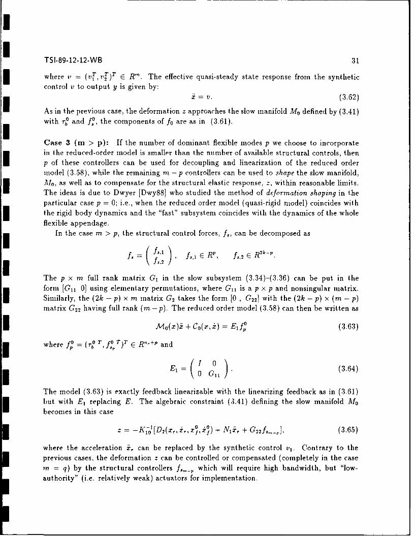
ITSI-89-12-12-WB 31where v (vT,vT R. The effective I -steady state response from the synthetic
1 -7- E R.Teefciequasi-tdy rsoe
control ty to output y is given by:xi = v. (3.62)
As in the previous case, the deformation z approaches the slow manifold M0 defined by (3.41)with r and f,, the components of fo are as in (3.61).ICase 3 (m > p): If the number of dominant flexible modes p we choose to incorporatein the reduced-order model is smaller than the number of available structural controls, thenp of these controllers can be used for decoupling and linearization of the reduced ordermodel (3.58), while the remaining m - p controllers can be used to shape the slow manifold,
110, as well as to compensate for the structural elastic response, z, within reasonable limits.
The ideas is due to Dwyer [Dwy88] who studied the method of deformation shaping in theparticular case p = 0; i.e., when the reduced order model (quasi-rigid model) coincides withthe rigid body dynamics and the "fast" subsystem coincides with the dynamics of the whole
flexible appendage.In the case m > p, the structural control forces, fl, can be decomposed as
S= (fs ) ,f, f3 e RI f, 2 e R 2 -P"
The p x m full rank matrix G, in the slow subsystem (3.34)-(3.36) can be put in theform [Gil 0] using elementary permutations, where Gil is a p x p and nonsingular matrix.
Similarly, the (2k - p) x in matrix G2 takes the form [0 , G22] with the (2k - p) x (m. - p)matrix G 2 2 having full rank (m- p). The reduced order model (3.58) can then be written as
I Mo(x) + Co(x,.) = Elf ° (3.63)
where fo (rio f¢oV) r n d= 'b i --+P and
E ( 1 ) (3.64)i E = 0 Gil '
The model (3.63) is exactly feedback linearizable with the linearizing feedback as in (3.61)but with E1 replacing E. The algebraic constraint (3.41) defining the slow manifold M0
becomes in this caseS-K-[D 2(X,, ,,X0,) + Nli, + G22f,,,-,, (3.65)
where the acceleration ;,. can be replaced by the synthetic control vl. Contrary to the
previous cases, the deformation z can be controlled or compensated (completely in the case?n = q) by the structural controllers f,, which will require high bandwidth, but "low-
authority" (i.e. relatively weak) actuators for implementation.

TSI-89-12-12-WB 32
3.1.4 Partial feedback linearization of the Reduced Flexible Model
In some applications, and depending upon the choice of the scaling, f may not be "small"
enough relative to the decoupling requirement. In this case, it is necessary to replace thequasi-rigid model (3.58) by the more accurate FOCM (3.57) for control design. The appli-cation of feedback linearization to the FOCM introduces a correction term in the controlswhich improves the decoupling (and thus linearization) of the system by an order of 6. Thecorrected controls are obtained via an expansion;
f = fu + ef, (3.66)
where f0 is the linearizing torque for the quasi-rigid (zero-order approximation) model.
Design of the corrective control f': The corrective control fl is designed to improvethe decoupling by annihilating the O(e) terms in (3.57), i.e.,
[Mi(x,ho) i Cl(r,.', ho, hJo, o) - Ef'] = 0. (3.67)
The construction will depend, as in the previous section, on the values of p and m. In thecase m < p the corrective control, f', can be constructed to annihilate part of (3.67). In thecase m = p, (3.67) can be exactly annihilated by:
f 1= E-1 (Ci(X, i, ho, ho, ho) + Mi(x, ho)v) (3.68)
If we apply the control, f = f 0 + Ef', to the reduced flexible model (3.54), where Tb, r,f,and f,' are as designed above, we obtain:
I = 17 + O(E 2 ) (3.69)
which linearizes the reduced flexible system up to order E
3.2 Conclusions and Directions
The results described in this section represent a preliminary analysis of the problem of PLFcompensation for multibody system with flexible interactions. (A preliminary version of theanalysis was presented at the 1989 American Control Conference in Pittsburgh, PA [ABB89].
Our interest in this phase of the research was primarily motivated by concerns for the com-plexity of implementation of PLF compensation required for high order FEM models of theelastic response of a multibody system. The primary objective was to demonstrate rapidslewing and precision pointing of the system attitude as defined relative to a body-fixed frameattached to the primary system body. The analytical approach based on integral manifold
methods offers a refinement of the standard singular perturbation approach which suggeststhat higher order corrections applied to the rigid body torques can improve performance of
PLF compensation for relatively low order models of structural flexure. Simulation studiesperformed during this study did not reveal substantial improvement from such corrections.
In response to the observed responses of simulation studies we can draw several conclu-sions. The SBL system model developed in this study consists of a multibody system with

I
I TSI-89-12-12-WB 33
primary system outputs to be regulated consisting of rigid body positions and parasiticsarising from low mass structural interactions. Primary system controls are collocated withthe position coordinates for regulation. Singular perturbation analysis reveals that the sys-
tem flexure dynamics in such cases are only weakly controllable in the sense that control ofthe fast time scale enters only through the slow time system. As is well known, such systemwill require additional control authority to affect control of the fast time scale response.
For the problem of rapid slewing and precision pointing this means that active structuralcontrol which interacts with the low mass density, structural components may be importantin achieving enhanced robustness of the system slewing and alignment responses. This ob-servation is potentially important given the increasing reliance on passive damping methodsfor space structure applications [RR87]. Unfortunately a comprehensive study will requiresome analysis of emerging technology for imbedded actuation and sensing of flexible struc-ture response. This was viewed outside the scope of the second year effort on the subjectcontract.
IIIIIIIIIII

TSI-89-12-12-WB 34
4 Some Design Approaches for Combined Rapid Slewing andPrecision Pointing
Consider the general form of the equations of motion for a multibody system undergoingattitude reorientation. The model includes n degrees of freedom (including elastic degreesof freedom retained from a FEM expansion) with position coordinates q E R' and velocitiesp E W .The model has the form,
q f(q)p (4.1)
mlq)p B(q,p)p + K(q,p)q = Gf (4.2)
where M, B, K are n x n symmetric, matrix-valued functions and G is an n x m. matrix.The n.-vector f includes generalized forces (and torques) acting on the multibody system.For simplicity we assume the position coordinates are ordered as: q = [ 7 T, T]T where-y E 3 parametrizes the rotation of the body fixed frame of the system principal body.Also, p = [w T , IjI]T , where w is the body angular rates. The general model includes nonlinearkinematics (4.1) which is assumed to have the form,
(q) =~ j 0 ,_
where the 3 x 3 matrix is defined previously depending on the parametrization of SO(3).The general problem of control of system pointing and inultibody alignment is addressed
by establishing a set of m principal system outputs taken as an in-vector of position coordi-nates,
y = C'q. (4.3)
Claim 1: The decoupling/PLF control
f = (CfA1Gy 1 v - (CF A1'G)'CTA1 1[(MD - B)p -Kq], (4.4)
with
D() [TW3 03,n-3D() 0,n-3,3 0n-3,n-3 '
renders the input/output response from v - y as a linear, 2m-dimensional system of theform,
=V.
Proof: To obtain (4.4) we proceed by direct computation of the normal form coordinates forthe general model (4.1)-(4.2) with outputs (4.3). First, identify a change of state coordinates,
(T)((), q)(
z T (q

TSI-89-12-12-WB 35
[O,0 C]' f(q) ( (4.5)Z, Z2 I
with Z1 , Z 2 chosen so that T has rank 2n. Thus a direct computation yields,
-1 = Cq (4.6)
z, = C'qt = CT(q)p (4.7)
= Ziq + Zir(-)p (4.8)
an invertible transformation.Before we obtain the system model in the (z, ) coordinates we express the accelerations
in a convenient form. From (4.1)-(4.2) we have,
q = --q = -{F(q)}q + F(q)P. (4.9)
Note that the n-vector valued function,
a- a-{F=(q)pl4 - {I(q)p}F(q)p (4.10)
[ Pr-w}l 0] [IN1) 0]() (4.11)
A principal advantage of the use of the Gibbs vector parametrization for attitude positionis the simple algebraic form of the kinematic relation. Appendix A establishes the following
based on the Gibbs vector parametrization,1{0o w}( 7 w= w(yw
Using this relation we obtain,
[~ r-~. I ] - [ (-Y) o ] A(q) -{fBp + Kq - Gf}1 (4.12)/=0 - 0 1n-3
= P(y)M(q)-f{[AI(q)D(q) - B(q,p)]p- K(q,p)q + G f} (4.13)
where,
D(q) T 01 0 "
Thr' model can be cxpresse- in normal form coordinates as,
- r(4.14)
Z2 = A(z, )13(z, )f, (4.15)
= F(z, ). (4.16)

rI
TSI-89-12-12-WB 36
From (4.5), (4.13) we have,
A(q,p) = f(y)M(q)-'{(M(q)D(q)- B(q,p))p- K(q,p)q} (4.17)
13(q,p) = F(y)M(q)-'G. (4.18)
The decoupling control is then,
f = 1(p,q)-i{ v- A(p,q)},
and (4.4) follows.
Claim 2: Given the model (4.1)-(4.3) we can find (n-m) x n valued functions ZI(q), Z2(q)
such that
Z1 F(q)M(q)- 1CT = 0, (4.19)
Z2 F(q)M(q)-ICT = 0, (4.20)
andC 0
T(q) : 0 CZ,(q) Z 2 (q) I
is nonsingular.
Claim 3: In the case that outputs for regulation, linearization, and decoupling defined by(4.3) are collocated with the generalized control forces; i.e.,
span{G} = span{CT}
then the (output-constrained) zero dynamics are given as,
" F(z.- )j=. (4.21)
where F(z, flpq) with (p, q) such that
w e () f () q, )(4.22)
and
f(p,q) = Z,(q)q + Zl(q)I(q)p+ Z2 (q)r(y,)p
+Z 2(q)F(q)M-{[M(q)D(q)- B(q,p)]p+ K(p,q)q}. (4.23)

TSI-89-12-12-WB 37
Proof- From (4.13) and (4.5) we obtain = Zq+ Z2. Direct evaluation of (4.16) obtains,
Z:(q)q+Z1(q)q± + Z 2(q)f(-y)p (4.24)3 +Z 2(q)F(y)M(q)-'{[M(q)D(q) - B(q,p)]p- K(q,p)q + Gf}. (4.25)
Then by Claim 2 and the assumption we have,
Z 2(q)F(-f)M(q)-G = 0.
4.1 Practical Implementation of Time-optimal Slewing for an Inertial Load
The advantage of the PLF control which implements the system inverse is the slewing controlcan now be implemented in the new coordinates. A switching control law is designed for theindependent decoupled axis motions in acceleration coordinates. The decoupled single axisresponse obtained after PLF compensation is:
(t) = a(t) (4.26)
where 0 is the attitude parameter for ith axis (subscripts suppressed) and a (the acceler-ation) is the control. Requirements for rapid slewing suggest a minimum time criterion isappropriate for the design of control laws.
Necessary conditions for a control law, optimal with respect to a minimum time objective,can be obtained directly from the maximum principle. Under magnitude constraint on theavailable acceleration,
Ia(t)l < amax (4.27)
the optimal control is of bang-bang type with switching strategy described by a switch-ing surface in the state space 3?2 with coordinates x = [9, . For the double integratorplant the optimal control involves determining a single switch point. Briefly, the optimalswitching surface is a quadratic curve in W?2 which can be obtained as follows. For constantaccelerations, a(t) = am,,x, the natural trajectories are,
9(t) = i + amt, (4.28)
0(t) = 60 + t + 2amaxt 2 , (4.29)
where 0(0) = 0 and 9(0) = are initial conditions. The optimal trajectory reaches the equi-librium at the origin in ninimum time. To identify the required switching surface choose thetrajectories which reach the origin at time t t by solving the above equations simultaneouslyand eliminating dependence on tf, to obtain,
S= 2amx ,. (4.30)
It is easy to see that the required switching surface in the state space R?2 with coordinatesz = [0,9]T is
.s(z) = f(z 2 ) + 2a.....zi = 0, (4.31)

TSI-89-12-12-WB 38
with f(z2) = Z2 1Z21 and the time-optimal control is bang-bang;
Ca(t) = -amax sgn{s(z)}. (4.32)
However, any practical implementation of the time-optimal control law will involve an ap-proximation of the ideal discontinuous actuation. Most realistic actuators have slew ratelimits, dead zones, delays, or other dynamics which may play a role in implementation dy-namics. A simple example of the difficulty of implementing time-optimal control can beillustrated if we replace the ideal signum function with a saturating element. In this caseit can be shown that the origin is not an asymptotically stable equilibrium. To see thisconsider a Lyapunov function,
V(z) = .TZ
defined on W2 with coordinates as given above. For the practical control law,
c(t) = -,,sat{s(z)}, (4.33)
where { , for _ 1/g,sat() gi , for 1 < 1/gi (4.34)
-1, for ! < -1/1
where gi is a positive constant gain representing slew rate limiting in the actuator.In a neighborhood of the origin such that Iz21 < 1/g we can evaluate the time derivative
of the Lyapunov function along trajectories of the closed loop system;
IT,; (4.35)
ST{[0 1] []sat{2amnxzz 2 z2 I}} (4.36)
-T 21 Z. (4.37)
The V-function is positive definite, decreasent, and radially unbounded. In the neighborhoodof the origin we have 1V < 0 for 1.21 < 1/g1. Any finite precision implementation of f(z 2 )
will ultimately become negligible near the origin and the closed loop system response willultimately oscillate with frequency V and amplitude given by the precision of f nearthe origin.
The above limitations are simple examples of the general tradeoffs involved in designof nonlinear control systems where dual mode operation must be considered to resolve thetradeoffs between requirements for static accuracy such as local stability, noise rejection, etc.and dynamic accuracy such as speed of response. These issues are well known to controlengineers but do not receive a lot of attention in the theoretical literature. Considerationsfor dual mode operation in this case suggest that the optimal switching function be replacedwith a dual mode version which approximates time optimal operation for large signal motionbut achieves asymptotic stability of the origin for small angle displacements. Additionally,considerations for small signal overshoot, stability margins, etc. can be included withoutsacrifice of the large signal response.

TSI-89-12-12-WB 39
A dual mode version of the time-optimal control law can be obtained by replacing thenonlinear function f with a peicewise continuous modification with finite slope near z2 = 0.
The choice,[ z+- for z2>g2 /2
2+9;,for Z2 <-g 2/2f(z 2 ) := 22, for 1z21 < 92/2 (4.38)
obtains asymptotic stability of the origin for any 92 > 0 with closed loop control (4.33).The resulting practical implementation of the time-optimal servo control law is shown
in Figure 4.1. Here 0, is the commanded attitude angle. To the extent that practicallimits of actuators permit, the gains g' and 92 should be chosen to satisfy local stabilityand overshoot as well as large angle rapid (time-optimal) slewing. These tradeoffs can bereconciled by appealing to the ideal bang-bang control law (4.32) with the modified f. Withideal switching the surface, s(z) = 0, (4.31) is an integral manifold for the closed loopsystem. From the theory of discontinuous differential equations we can obtain stabilityanalysis by decomposition of the closed loop system dynamics into two phases: 1) reachingto the switching surface and 2) ideal sliding on the switching surface.
Assume the closed loop system achieves ideal sliding condition s(z) = 0 for t > t,. Thenthe sliding dynamics are obtained from the constraint (z) = 0 for t > t,;
S(Z) = f'(z2)2+ 2amx.i = 0
where f = Of/&z2 . In the linear region of the peicewise function f-namely, when Iz21 <g2 /2-we obtain,
, s(z) = g2a + 2am,,z 2 =0. (4.39)
The equivalent control in sliding is
arq = - Z2. (4.40)92
The sliding dynamics on the manifold M, = {z E g2 : s(z) = 0} are then obtained bysubstitution of the equivalent control in the closed loop equations. In the linear region weobtain,
1= 2 (4.41)
2= 2 (4.42)
and together with the constraint s(z) 0 the ideal sliding dynamics reduce to
"2 = 2 Z2 (4.43)92
which are asymptotically stable to Z2 = 0 for any 92 > 0. The local time constant in sliding
iss 92 (4.44)
2ctmax

TSI-89-12-12-WB 40
To choose the gain 92 we take 01 as the desired tolerance for large angle slewing; i.e., forany initial offsets exceeding 01 we want to apply large angle, time-optimal slewing control,but for any offsets smaller than 01 we want linear mode action. Then the required gain isobtained by substituting z= 01 into (4.31);
92 = V2Oamax81 (4.45)
The resulting linear mode time constant is
IA" 1
Note that the ideal sliding dynamics retain the feature of no overshoot characteristic oftime-optimal slewing into the linear mode operation.
To implement the time-optimal servo we need to understand the limits of saturation
mode operation of the actuator and the effect of available torque. From the theory of slidingmode design it remains to show in what region sliding will be achieved. A straightforwardapplication of the reaching analysis of [DZM88] follows. From (4.31) let V(z) = ls2. To
achieve sliding we need to show that sis < 0. Here
. (z) f'(z 2 )z 2 + 2mamx'i (4.46)
whereOf 2z 2 , for Z2 > 92/2
f Z_2- 92, for IZ2 1 < 92/2 (4.47)-2z 2 , for z2 < -g2,/2
A necessary and sufficient condition for sliding to be achieved globally with the ideal switch-ing control law
a(t) = -a.,tXsgn{s(z)},
is
amax > amnax
Within the linear region sliding is achieved when
amax > >_amx.
For practical implementation of time-optimal slewing the choice of actuator slew rate giis critical. With the (practical) closed loop control (4.33) the dynamics in a neighborhood
Sof the origin are given by [ 0 1 1= 2 1x z. (4.48)
Sensitivity of the stability properties can be determined from a root locus analysis withU respect to gi (see Figure 4.2). The characteristic equation of the closed loop system is
A2 + tmax99 2 ,\ + 2Ca~Xgj = 0I

TSI-89-12-12-WB 41
Figure 4.1: Implemenation of Time-Optimal Servo
1.7
a Z
Figure 4.2: Root Locus for Linear Mode Sensitivity of Saturation Mode Slewing
which we write in the formA2 + k(g 2A + 2amx) = 0
with k = amaxgi. To approximate ideal sliding in the linear region we require
8g, > -
which guarantees that the roots are real and stable. As g, > 0 is increased the smallsignal response is dominantly a single time constant which approaches the ideal slidingmode response in the limit as g, - oo [SS83].
4.2 Implementation of Rapid Slewing with Coordinated Modes of Actuation
In this section we describe the basis for design of coordinated use of different modes of ac-tuation for rapid slewing. The idea is to utilize the smooth (or continuous) mode actuators(such as AMED's) to implement a component of the PLF compensation. This implemen-tation permits a simple decomposition of the slewing control into individual single axiscommands. The slewing control is implemented using discrete (discontinuous) mode actua-tion (such as reaction jets). This is consistent with the very large torque requirements forlarge angle, rapid slewing of significant system inertias. Bang-bang mode operation of high

TSI-89-12-12-WB 42
torque AMED's (such as reaction wheels and CMG's) is inconsistent with (or at least tech-nically very challenging for) the state-of-the-art. Whereas reaction jets can-depending onphysical placement issues-generate very large torques with rapid, discontinuous action; buttheir use in throttled (continuous) mode is technically challenging. The decomposition ofcontrol authority suggested in the following design approach is chosen to exploit the benefitsof current actuation technology for attitude control.IOne design approach for rapid slewing focuses on controlling the dynamics of the rigidbody motion. We discuss the implications of dynamic reaction from the elastic appendagein the context of robust control performance. Recall that the rigid body dynamics can be
given in the form,
(y)-,b Wb) +(4.49)
Wb = IT'(Ib X b) + 61b (4.50)
where -y, wb G '3 are respectively the vector attitude parameters and angular rates referencedto the body fixed frame.
To control the vehicle attitude we now design an implementation of PLF compensationfor the system outputs,
given the external torques, rb, applied to the rigid body. We remark that the assumptions
leading to the model (4.50) together with the choice of primary system outputs, y, indicatethat the relative degree from each input/output pair, rb,i -- yi is 2. Transformations obtainedas in (2.27) indicate that the system can be exactly linearized by feedback (i.e., no zero
dynamics are obtained in the transformation to the normal form).The computation of the normal form coordinates is obtained as in section 2 by differen-
tiation of the output. In this case,
z1 = Y = ?(4.51)
Z2 = y = r(-y)w (4.52)
and since the 3 x 3 matrix F is nonsingular for almost all -y the transformation is invertible.A straightforward computation obtains the normal form as,
Z I =-- Z2
2 = A(zi, z 2 ) + B(ZI, z 2 )r (4.53)where
B(z,) = F(z)IC' (4.54)
A(zm,- 2 ) = + ×(-),'bw x w)] (4.55)
IThus the feedback compensation which linearizes the system (4.50) for large angle motionis [Dwy84],
r b B(zi)-'{ a(t)- A(- z, )}
ST -IbWW - Ibw X w + Ibr()a(t) (4.56)

TSI-89-12-12-WB 43
where a E R3 is the "synthetic control" (in acceleration coordinates). To implnment therapid, large angle slewing control we apply the bang-bang, time-optimal switching logic toeach axis; i.e.,
a, -a,x sgn{f(z2 ,i) + 20OmaxZlii}
as in (4.32) with f(.) as in (4.38). This form assumes identical acceleration limiting is desiredin each axis.
A straightforward computation reveals that we can write,
A(zi, z2 ) = B(zi)d(z1 , z 2), (4.57)
withd(zi, z 2 ) = [_Twlbw + Ibw x w] .=, w=r(z,)Z2 (4.58)
The normal form equations can be written,
- 2 (4.59)
L2 = B(z1,z2){d(z,,z 2 ) + Tb}. (4.60)
Note that the factorization obtained in (4.57) indicates that the matching condition forrobust feedback linearization is valid for the model terms contributing to d(z1 , z2 ).
One approach to implementation of feedback linearizing control for rapid slewing is toimplement the compensation in two components;
Tb = 7C + -r, (4.61)
where the continuous mode torque component is,
7 = -d(zi, Z2)I ,=.,=r( )w
= -[TIbob + IbW x w]. (4.62)
This component compensates by decoupling the Coriolis and centripetal accelerations arisingfrom large angle, rapid, rigid body rotations. Note a typical source of model uncertaintyarises due to asymmetries in system inertia properties which are typically not considered incontrol system design studies. Such asymmetries arise in the SBL system with the additionof trackers or additional mirror components. We see that the smooth control is not directlydriven by the subsequent synthetic control which obtains the desired slewing maneuver.Thus the smooth control functions to reliably achieve linearization.
The second component, r7, will be implemented by discontinuous or saturation modeactuation. We shall now indicate a simple approach to identify a switching control law forr' based on VS control design. After application of the control (4.61) to (4.60) we obtainthe design system for the choice of the saturation mode control law,
z1 = Z2
2 = B(z 1,z 2 )r (4.63)

TSI-89-12-12-WB 44
For design of VS control we follow the method described in section 2. Thus we choosethe switching surface in the normal form, z-coordinates. The choice of the switching surfaceestablishes the ideal dynamic behavior in sliding and its design should embody the systemdesign goals. In section 2 and [KK89] we outlined options for stabilization of the origin. In thepresent design the large angle slewing motion is critical and the design goal is time optimalmotion. Solution of the general problem of time-optimal attitude control for the rigid bodyequations (4.50) with independent saturation constraints on the available torques, Ifi < 7m.x
is an open problem [AF66]. The formal time-optinial control problem does not embodyconsiderations for robustness or implementation issues as described above and we will notconsider it further. Our approach is to develop requirements for the torque authority of thesaturation mode control, r, so that decoupled, independent single axis slewing is obtained.
In section 2 we showed that, in sliding, the inverse dynamic control which linearizes thesystem response is obtained implicitly. The PLF also obtains decoupling of the individualresponse of the motion about each axis. Our approach is to choose the switching surfaces forindependent axis slewing by applying the modified, quadratic switching surfaces for time-optimal servocontrol (4.31) to each axis.
To make these statements precise we introduce the following notation. In the normalform coordinates we decompose the positions and rates in terms of decoupled axis motionsas,
(Zk' IZk Zk, 2
Zk,3
for k 1, 2. Then in the normal form coordinates we establish three switching surfaces,
si(z) = f(z 2 ,i) + 2a 1,, Zi
for i 1,... ,3. Let s(z) = [s,s 2 ,s3S ' .
It is easy to see that if we can enforce the sliding mode over a significant region of theswitching manifold, M, then the independent axis, time-optimal slewing will be obtained.The design of the required switching control to achieve sliding on M, and to guaranteereaching the manifold from the expected region of operation after a sufficiently small transientcan be based on Lyapunov stability arguments as follows.
Consider a V-function,
v =
defined in the normal form coordinates. The time derivative of V along trajectories of (4.63)is,
V. = T(() = e9s.
= sT(Z)[2m.txI 3 , F'(z)] B(z)rT
= T(z){2an,xZ2 + F'(z)5(z,)r'}, (4.64)
whereF'(z2 ) diag{f'(z2,i), i = 1,2, 3}, (4.65)

I
U TSI-89-12-12-WB 45
{ 2 , for 9>g2/2f) g2, for I1 < g2/2 (4.66)
1-2 , for _< -g2/2
To guarantee that the switching manifold is reached in finite time and that sliding isachieved we seek the control law which satisfies,
min sT(z)F'(z)B(z)rs < -it (4.67)
for it > 0 with admissible controls
Tad = {17 E R' 17 i 1, 2, 3}. (4.68)
Claim 4: The saturation mode control law which is optimal for (4.67)-(4.68) is,
rs = - Tmax sgn{BT( zi)[F'(z2 )]Ts(z) } (4.69)
for i = 1,2, 3. Together with the optimal switching strategy (4.69) a sufficient condition forthe required saturation mode control authority to guarantee that V < 0 in a given closedset, y E B , containing the origin is
Tnm . max,=,, 3 ,nax B, =,[1(-y)i']-' (4.70)
Proof: From (4.64) it is sufficient to show that
TmrX > max max [ 2ai= ,,3 Y S I 3 rf-j t [ ( 2L Zl l'
From (4.65)-(4.66) and (4.54) we can simplify the ratio for each i as,
2ckmaxIZ'2,il _ 2amax IZ2,i IIZ =1 [F'(z2)B(Z1 )]ijl I I f'(Z2,,)[r(.z,)I '],jI "
To find the worst case for each i from the discontinuous definition (4.66) we note that forIZ2,il > g2/ 2 ,I If'(z 2,I 2Iz2 JI
and for the case Jz2.ij < 92/2 ,
I 2a,.ex 12,Ij 2amxIz2,uI-2,1 /2 If'(Z2 ,)I - = max.0
I0

TSI-89-12-12-WB 46
2ana +----- iij et A ttitu d e
i AMED's Dynamics --
Figure 4.3: Coordinated Rapid Slewing Control Implementation
To obtain the required strict negative requirement 1V < -i similar relations can be de-veloped which involve assumptions on the a priori maximal rates, IZ21 < imax. Our principalconcern is in implementing the bang-bang control with sufficient control authority Tmx,, suchthat reaction of the flexible appendage response will be effectively decoupled from the rigidbody attitude so that time-optimal slewing can be obtained. Note that the control law(4.69) can be implemented independently of state measurements associated with the flexibleappendage deformation. The overall control structure is illustrated in Figure 4.3. Fromthe above analysis we see that robustness to model uncertainty can be obtained if sufficientcontrol authority in slewing torque r' (in particular T.A. is large enough) is available so that(4.70) is satisfied for all model variations [GP82].
4.3 Coordinating Control for System Slewing and Multibody Alignment
Throughout the modeling and control development for multibody slewing we have empha-sized the importance of establishing a body fixed coordinate system attached to a systemprimary body. The dominant system nonlinearities arise from the introduction of nonlinearkinematics and dynamics of large angle rotations. We have implicitly assumed that struc-tural deformation contributing to multibody misalignment dynamics are small and thereforelinear when referenced to the body fixed frame. Our approach for coordinating multibodyalignment and rapid slewing will be based on these assumptions. We now show that appli-cation of PLF compensation for linearizing and decoupling the natural nonlinear responseof rapid, large angle slewing motions of the system primary body results in decoupling themultibody alignment problem from the slewing problem.
Referring the general multibody dynamics model (4.1)-(4.2), consider now the specialcase of (5.47)-(5.52). Let q = [yT, uT]T, p = [wT,itt]T, and it = [ TT]T. Then the SBL

TSI-89-12-12-WB 47
model for multiaxis slewing developed in section 5.1 can be written in the form,
[l 1 i(q) All 2(q) )(b ) + r B, 1(q, p) B12(q, p) 1 . b
Ii'(q) A' 2 2 (q)]~i, B'(q, p) B22(q, p) j~'J~K' (q,p) K 22(q,p) u 0
We focus attention on the regulation of the primary system body frame attitude and takeas primary system outputs,Oq = C-,
where we assume that y and 7b are 3-vectors and the 3 x 3 matrix C, is full rank. We furtherassume that the regulated outputs (note that, these outputs do not necessarily coincide with
sensor locations) are collocated with the primary body torques;
C, -- Grb.
Under these assumptions it is by now easy to see that the zero dynamics resulting from PLFcompensation are given by,
M22 u + B 22ii + K 22u = 0. (4.72)
Note that (4.72) is linear time invariant equation of the free response of the multibody
alignment and structural vibration with
I 7=-W=0.
Stability of the zero dynamics is a prerequisite for stabilization using PLF, but for practicalimplementations the degree of stability may be an important factor. For the SBL rapidslewing and pointing problem this decomposition of control problems is critical to systemperformance.
Decomposition of Control Authority and Stabilization of the Zero Dynamics.Consider the general model of (4.1)-(4.2) modified to include additional controls,
41 = L(q)p (4.73)
A(q)p + B(q,p)p + K(q,p)q = Gbrb + Gf, (4.74)
primary control alignment control
A direct computation based on (4.4) indicates that the required PLF compensation forthe output (4.3) includes feedforward from the structural controls;
T b= (Cfl'Gbr-V - 0CFM'Gb)1 CfAr'[(MD B)p - Kq + G ~f, (4.75)
and the resulting zero dynamics are
AI22ti + B22 + K221 = G, (4.76)

TSI-89-12-12-WB 48
For application to rapid slewing of the multibody system the primary system output willbe taken to be y = b (or in terms of the Gibbs vector y = y ). Referring to the equations of
motion for the generic multibody system derived in Section 5.1 we see that the zero dynamics
(4.76) are merely the linear dynamics of the flexible structure with cantilevered boundary
conditions. The structure controls effect multibody alignment and vibration suppression
relative to the system body fixed frame.
The design approach we suggest is the integration of precision multibody alignment and
vibration suppression based on robust stabilization of (4.76) together with the PLF compen-
sation and slewing design described above. We remark that the design approach is predicated
on the fact that multibody alignment for precision pointing and tracking is required at thetermination of the slewing maneuver. Stabilization of (4.76) by the introduction of local feed-
back will effect transient responses during the slewing maneuver but the principal concern
is stabilization at the end of the slew.
Remark: The decomposition for coordination of multibody alignment with rapid slewingcan be viewed as a generalization of implementations commonly used for vibration suppres-
sion in flexible space structures. As described in [Jos89] implementation of feedback control
for active vibration damping commonly uses pairs of actuators and sensors symmetrically
located so as to eliminate sensitivity to rigid body modes. Such configurations are required
since the low levels of control authority typically available for structural damping are too
small to effect attitude and translation of the space vehicle. If the response of the rigid
body modes are not decoupled from these control loops the actuators would saturate during
any maneuver. Although the approach based on PLF for decoupling clarifies the role of
local linear mode vibration damping in the context of the nonlinear system dynamics. Note
however that in general, stabilization of the local linearization of the zero dynamics may not
guarantee global stabilization with feedback linearizing control [KS89].

TSI-89-12-12-WB 49
I5 Simulation Tradeoff Studies for Multiaxis Slewing of SBL Sys-tem Model
In this section we develop a model for generic SBL system beam expander as a two bodysystem with elastic support structure. The model is refined from that developed and reportedin [BBKA881 by:
* 3 rotational degrees-of-freedom included in system primary rigid body motion,
* area moments of attached structure modified to represent tripod metering truss,
* system inertias and slewing requirements scaled to represent capabilities of ASTREXfacility and initial test article.
5.1 Multibody System Model for Multiaxis Slewing and Precision Alignment
The modeling method of Lagrange's equations, as described in the report [BBKA88], alongwith spatial discretization via collocation by splines to develop a finite dimensional model
suitable for simulation of large angle. multiaxis motion of a generic, two-body model of aSBL system beam expander is described in this section. Beginning with the generic flexiblespacecraft model [BBKA88, sec 4] the following model assumptions are made:
1. axial appendage deformations are negligible, r73 - Z,
2. translation velocity of the system primary body is negligible, R _ 0,
3. torsional appendage deformations are negligible, V,(z) ;-, 0.
Thus, following the DPS modeling approach discussed in [BBKA88, sec 3], the configurationspace for the distributed parameter model is SO(3) x H1, where Hg is the set of continuously
I differentiable functions, x(z) = [77 1, 7 2 ,h]T e H1 defined on the interval z E [0, f], andwhich satisfy the geometric boundary conditions
G : 771(z)= 0, 77 2W =0, O(z)=0, O(z) = 0, at z =0.
With the notational conventions in [BBKA88], the model will be described by the appendagelateral deformation, 7 (t, Z) = 771, ?2]r , along the body-fixed x and y axes, respectively, andappendage angular deformation, (z, t) = [O(z),k(-)]T. The attitude angular rates referencedto the body fixed frame are denoted, Wb.
The potential functions for the variational analysis leading to the dynamic equations ofmotion reduce in this case to:
T = t 4 IbWb (5.1)
f °jIb?7(=) + 7 (Z)II 2pA dz
+ j[Wb + PS(z)TI[Wb + Pt(z)]p dz,I
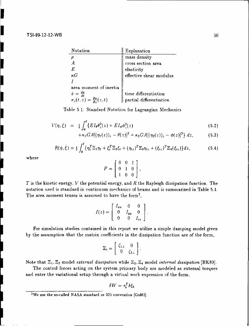
TSI-89-12-12-WB 50
Notation Explanationp mass densityA cross section areaE elasticityKG effective shear modulus
Iarea moment of inertiai -_ d time differentiation
dtXz(t, z) =(zt) partial differentiation
Table 5.1: Standard Notation for Lagrangian Mechanics
1,{EI1#2(z) + EI €0(z) (5.2)
+KIGA[(771(z))z- 9(z)]2 + K 2 GA[(712 (z))- - (z)]2} dz, (5.3)
R7 = / {rhT'm + 'T:27t + (ltz)Esllt + ( -t')-.4 (tz-)}dz, (5.4)
where
[0 0 JP= 0 1 0,
1 0 0
T is the kinetic energy, V the potential energy, and R the Rayleigh dissipation function. Thenotation used is standard in continuum mechanics of beams and is summarized in Table 5.1.The area moment tensor is assumed to have the form2 ,
1.. 0 0
I(z) f 0 IU 00 0 1-.
For simulation studies contained in this report we utilize a simple damping model givenby the assumption that the matrix coefficients in the dissipation function are of the form,
1i~ 0]-i= 0 (2,i "
Note that E1, 2 model external dissipation while --3, '-4model internal dissipation [BK89].The control forces acting on the system primary body are modeled as external torques
and enter the variational setup through a virtual work expression of the form,
8W =rbS6
2 We use the so-called NASA standard or 321 convention [Gol82].

TSI-89-12-12-WB 51
In the sequel, we refer to the kinetic energy expression in terms of three components;
Trigid body = lwTIbwb, (5.5)
Tflexi = 2 fr 2b7(z) + il,(z)jj'pA dz, (5.6)
Tflex 2 ---- j [ b + _t(z)]Tl[Wb + -t(z)]p dz. (5.7)
5.1.1 FEM: Collocation by Splines
A model based on the Finite Element Method (FEM) is obtained by spatial discretizationvia collocation by splines. The use of splines for such purposes is described in [BBKA88].
Given the geometric boundary conditions described above the discrete approximations of thescalar valued functions, 71 (z),i72(z),0(z),O(z), are decoupled and reduce to approximationof a single scalar function, say -(z), on the interval z G [0, ej with boundary condition,y(0, t) = 0. Dividing the interval [0, t] into N uniform subintervals and using first-order
B-splines we obtain the approximation:
* N-t(z,t)j (t ) i- z (5.8)
with the boundary condition, = 0
N
Si (t) Bil-1(0) = 0.Ii=OThen following the reduction procedure described in [BBKA88, §4.4.2] we obtain the FEMapproximations with 'f(z) as given in [BBKA88, Eqn. (4.47)],
771zt 0 'T'(z)ChOt (5.9)
772(Z, t) 't'( z)fl2(t ) (5.10)O(Z' t) tTe(z)O(t) (5.11)
(zt) qje(Z)¢(t). (5.12)
5.1.2 Reduction of the Kinetic Energy Function
Using the FEM approximations of order N we obtain the spatial discretization of the kineticenergy terms,
Tflex+ 2 r ( + 2 ( ± z.I} (5.13)
Tflex2 2 b +2J (5.14)
wherer N,,7r2 + Ir71 7 2
I.,,(i) - N,7 , 2 1 N,'N+ ,-j 2 + ] (5.15)_I N2_frN, r 2-r N,7, q2- +rN,,

TSI-89-12-12-WB 52
NM=fpA4( Z) T( z) dz, (5.16)
NT = f'pAz42'(z)dz, (5.17)
0. j o pAz 2 dz= -M (5.18)
- o -NT3,1-I17 NT7 0 ] , (5.19)
177N,71 ] (5.20)
JfPI(z) dz, (5.21)
J Nq2' 0 (5.22)
and
N19 0 ] (5.23)J = 0 NOO
The following terms are used in the above expressions,
N = pzj'(z) dz, (5.24)
N =pOT jpI ,pT(z) dz, (5.25)
NT = oPI (z)d, (5.26)
N,, = jpI.4 ,(z),T(z) dz, (5.27)
Nee = fo p.,p(z)T(z) dz. (5.28)
Note that the total kinetic energy can be written in the standard form,
2 b 7 t( (5.29)
where
M(1b , 1(,,77 0 . (5.30)J- [ 0 JI

TSI-89-12-12-WB 53
5.1.3 Reduction of the Potential Energy and Dissipation Functions
As above, the potential energy and dissipation functions are reduced by substitution of theFEM approximations. For the potential energy we obtain,
V=- 1 {OT Kj + TKO + T Kj,, + TIK,, + 2OT K,,7, ±2¢kTK i 2 }, (5.31)
where
Ke = f{EI A(z)(z) + KiGA1(z)¢r(z)}dz (5.32)
K, = {EI ,Dz(z) r(z) + K2GAI(z)$T(z)}dz (5.33)
Ki, = fiAk (T(zl- (5.34)
K, 2 = 'jlKGA¢z(z) T(z)}dz (5.35)
Ptt
TK2 = {KGA-t(z) (z)}dz (5.36)
ft{K2GAt :)r(z)}dz. (5.37)
Similarly, the dissipation function reduces to the form,T TT T
R B= 771 + 72j B±7 772 + 9 B9 + + B + 20 Bq,7 1 + 20 B ,7 2 }, (5.38)
where given the expressions,
Ro := 1O(Z)pT( z) dz, (5.39)
Ro := )4( z) dz, (5.40)
0R /f f .Z:=( ) (5.41)
we find it convenient to express the individual matrix coefficients in R (arising from the
FEM approximation) as:
B, = CiR 0 ± i3' for i = 1,2, (5.42)
Be = (6 2 + ( 13 )Ro + ( 14 R', (5.43)
BO = ((22 + ( 23 )Ro + 2 4 Ro, (5.44)
B1,1 = -( 1 3 Ro, (5.45)
B70= -, 23Ro. (5.46)
Finally, we summarize the model stiffness and damping using the expressions,
07 K , 0 K, K e ,1 0
B 7 . B77 2] B,74=Be, B0 B [ B ]

I
U TSI-89-12-12-WB 54
5.1.4 Lagrange's Equations
Finally, we compute the equations of motion using Lagrange's equations in the form:
q = f(q)p (5.47)
M(q)* ± [ 'M(q)] P- 1 [ (q) p T + -6V = _R + Qq (5.48)J9 2[ 9q 6P q P
with generalized coordinates q = {4, i, }, and velocities, p ={b, , -}-
Equations of Motion for Multiaxis Slewing Applying Lagrange's equation results
(after some simplification) in the equations of motion with kinematics of the system attitude
expressed in terms of the Gibbs vector, y;
-y = F('))wb, (5.49)
and kinetics,
Iw + I - }HTwb ± R + K.I ± K ± B, + B' = G H- (5.51)TI + "W- + -I-W +T 1-77 + T.4 +"--I +I.+J.]b+1,,7
J TLb + R + K7 + ±j + B + = G j , (5.52)
w here JT( b + + < 74 +j B =i(
- T NT 2 N , LTa-
2 - 3 T 2i, 1H= + 2 ±N77 -w,r,qTV - 2wL3N J (5.53)
w-7 3 20'N7rN + -W 2NT + w32? N.. +
R(wb) [ W3 N,, 0 ] (5.54)
5.2 Computer Simulation Model for Nonlinear Control Law Tradeoff Studies
A computer simulation model was developed and coded based on the above FEM model forattitude slewing of a flexible space craft (5.49)-(5.52). The model parameters and geometrywas chosen to represent the dynamics of a SBL system beam expander with structural
flexure arising from the flexure response of the metering truss. A goal of the second yeareffort was to develop concepts for experimental testing of nonlinear control concepts for
flexible space structures. A suitable facility for testing large angle, multiaxis slewing andprecision pointing is currently under construction at the Astronautics Laboratory. The
ASTREX facility with include 3 axis slewing and the initial test article is a scaled model
of a SBL beam expander. We have adapted our nonlinear slewing control simulation modelto represent available parameters and geometry of the ASTREX test article. Details of the
modeling assumptions and geometry are given below.

I
TSI-89-12-12-WB 55
5.2.1 Simulation model geometry assumptions and parameters
The objective of the simulation model design was to generate a simplified model that wouldduplicate, as closely as possible, the geometry and dynamics of the ASTREX test article.Information describing the test article was sparse, therefore, the following assumptions wererequired to develop a working simulation model:
1. The basic configuration of the model consisted of a rigid body, representing the mainmirror assembly and associated structure, and an attached tripod structure, represent-ing the flexible metering truss with secondary mirror, see Figure 5.1.
z
X
7RiJ5S
Figure 5.1: Simulation model.
2. The metering truss geometry consisted of a tripod of tubes located at the corners ofan equilateral triangular base. The generic model discussed above was readily adaptedto represent this geometry by including spatial variation of the area moments I,,(z)and I,(z) based on this geometry. Details of the computation of the area momentsand the resulting FEM model approximations are given in Appendix A.
3. The dimensions of the metering truss model were as follows:
Length, 1- 5.0 mBase width, b - 3.8 inTube inner dia. - 8.0 cmTube outer dia. - 12.7 cmMass of secondary mirror - 190 kg (5 % of total sys. mass)
4. The overall system characteristics were as follows:

TSI-89-12-12-WB 56
Mass moments of inertia 16640 kg m 2
IYY = 16590 kg in 2
Iz- = 11660kg in 2
System mass m = 3810 kgFirst modal freq. of metering truss = 12.2 Hiz
5. The dynamics of the secondary mirror were neglected and it was modeled as a pointmass at the end of the truss.
6. The modulus of elasticity of the truss material was chosen so that its first modalfrequency matched that of the ASTREX test article.
5.3 Simulation Results for PLF Control with Rapid Slewing and PrecisionPointing
Based on the above simulation model a digital simulation was developed using PC-Matlab
to perform tradeoff studies for implementation rapid slewing and precision pointing of an
SBL beani expander with PLF compensation.The model equations (5.49)--(5.52) with position coordinates, q = I', T, flT, and ve-
locities, p = b 17 IT, can be reduced to the generic form (4.1)--(4.2). The simulationmodels and parameters assumed for the tradeoff studies are summarized in Table 5.2. Sim-
ulated time responses for each model with several different control laws are displayed in
the figures contained in Appendix C. Each simulated maneuver is summarized in a set of
figures including the responses of position y, attitude rates, j, system torques applied to the
primary body, rb, and deformations at the apex of the truss, 7 ().(). Table 5.3 describesthe simulation runs performed and illustrates the relationship between system models and
control laws used.
Slewing with Smooth PLF Compensation. For precision pointing of the system at-titude we take the primary system outputs as y = -y. PLF compensation for the resulting
system is given by the formula, (4.4). Multiaxis slewing and pointing control was imple-
mented on an independent axis basis subsequent to PLF compensation. Thus the PLFSlewing control is obtained by setting the v controls appearing in (4.4) as,
Vi = i, for i = 1,2,3
where the commanded accelerations, cyi are generated by the independent axis, time-optimal
slewing control,ci(t) = -ct,,,, sat{f(,) + 2a,,..j'i},
as described in Section 4.1.
Simulation tradeoff studies completed this year focused on the implementation of PLF
compensation for various reduced-order models of the metering truss flexure. The reduction
methods described in Section 3 were used to obtain implementation alternatives for PLF
compensation in terms of the quasi-rigid model with DOF, r = 3, 4,,5, 11. The case r = 11

TSI-89-12-12-WB 57
Parameter Simulation ModelMODI MOD2 MOD3 MOD4 MOD5 MOD6 MOD7 MOD8 MOD9
SBL beam expander model parametersp - mass density 1520 -
E - elasticity 200 -
N - # finite elements 2 - - - - - - - -
c damping factor .001 .001 .004 .004 .001 .001 .001 .001 .001
?nt./mt,,t 0.05 0.0 0.05 0.0 0.0 0.0 0.05 0.0 0.05Control/Actuator parameters
,,x [rad/sec 2] .349 - - - - - - -
T111,X Peak Torque N/A N/A N/A N/A 9.3 1.4 27.0 22. 22.(x 103 )
g, - control gain (x 10') 6.477 6.477 6.477 6.477 5.E6 5.E6 5.E6 5.E6 5.E6
92 - control gain 0.0374 - - - -
Simiulation Solution Precision
ODE tolerance 0.001 -
Table 5.2: Matrix of Simulation Models Considered
Models Control LawsContinuous PLF/Slewing Disontinuous PLF/Slewing
r = 3 r = 4 r = 5 r = 11 Slew rate Discontinuouslimited torque torque
Multiaxis Slew
MOD1 SIMll SIM12 SIM13 SIM14MOD2 SIM21 SIM22 SIM23 SIM24MOD3 SIM31 SIM32 SIM33MOD4 SIM41 SIM42 SIM43MOD5 SIM51MOD6 SIM61 SIM62MOD7 SIM72MOD8 SIM81MOD9 SIM91
Multiaxis Large Angle Slew
MODI SIM1 SI1M16MOD2 SI1M25 SIM26
Table 5.3: Matrix of PLF/Slewing Control mnplementations

TSI-89-12-12-WB 58
U Slew Times (sec) to 1yij < .001PLF Model DOF
r= 3 4 1.5 11Model MOD1
Axis 1 .8005 .8218 .8268 .82582 .6709 .6725 .6933 .69303 .5145 .5162 .5241 .5223
Model MOD2
Axis 1 > 1.00 .8257 .8246 .82962 .8402 .8335 .6868 .68723 .5145 .5168 .5189 .5183
Model MOD3
Axis 1 > 1.00 .8260 .82732 .8497 .8494 .68923 .5172 .5193 .5227
Model MOD4
Axis 1 .8094 .8277 .83022 .6732 .6920 .68883 .5184 .5136 .5191
Table 5.4: Slewing Times for Standard 3-axis Maneuver
corresponds to compensation for all the simulated elastic degrees of freedom of the flexiblestructure response and was included as a baseline for ideal PLF compensation.
Simulation runs SIM11-SIM43 were made to compare slewing time and peak torquerequirements for implementation of PLF compensation for multiaxis slewing. For com-parison of subsequent time responses, a nominally small angle, multiaxis maneuver was
considered with desired system attitude given by -y = 0 and initial orientation given by-y = [.07, .05, .0 3 IT
. This attitude maneuver can be expressed in Euler angles as,
[V,, 0, ] = [1.40, -1.7°,2.3°].
Performance results for continuous mode PTF implementation are summarized in Ta-ble 5.4 and 5.5. The performance sensitivity to the presence of a significant mass (approx-imately 5 % of the system mass) at the apex of the truss was also examined. Despite therelative stiffness of the structure the multibody coupling is evident in the attitude overshootr'r the small angle maneuver. (All simulation runs are included in Appendix C.) hnple-mentation of the PLF compensation for multiaxis slewing requires increased bandwidth andpeak torques on the system rigid body. The importance of damping in the appendage can beseen in Tables 5.4-5.5. With increased damping peak torque required for PLF compensationwill decrease.
To illustrate the large angle response with PLF compensation we also simulated a ma-

TSI-89-12-12-WB 59
Peak Torque ATp(r)/Tpk(3)
Relative to rigid body casesimulation PLF Model DOF
model r 3 4 5 11MOD1 0 1.11 1.10 1.12MOD2 0 .278 .282 .293MOD3 0 .848 .842
MOD4 0 .238 .243
Table .5.5: Relative Peak Torque Increase with PLF Compensation DOF
neuver characterized by -y = [.5, .4, .3]T, which can be expressed in Euler angles as,
[V,, 0, 1 = [45.0, -19.50, 61.30].
The simulated time responses with PLF compensation for the rigid body modes only reveals
significant overshoot and in the case of a mass at the apex significant torque switching activityis generated. The addition of PLF compensation for the rigid body plus first two elastic
modes of the beam recovers ideal time-optimal attitude orientation. This also noticeablyreduces chattering activity near the time-optinal switching surface. For these large angle
maneuvers (probably difficult to test experimentally at the ASTREX facility) the lateraldeformation of the apex (with tip mass) is less than 1 cm. indicating the stiffness of thisstructure.
Slewing with Discontinuous/Continuous Actuation. Simulation studies SIM51-SIM91were performed using coordination of discontinuous and continuous modes of actuation for
PLF compensation and rapid slewing as described in section 4.2. The simulation trade-off studies for this case focused on the requirements for increased peak torque to recovernear ideal time-optimal, independent axis slewing using only the rigid body attitude output
information for control law implementation.
As discussed in Section 4.1 actuators are often subject to slew rate limits which willlimit switching response for on-line implementation of discontinuous mode control laws of
the form (4.69). Simulation runs were completed with slew rate limited implementation of
the discontinuous controls, r', by replacing the sgn function with a saturation function withlinear slope, g9 (cf. Table 5.2).
The significance of implicit PLF compensation achieved in sliding is apparent by com-parison of the time responses of SIM13 and SIM72. In both cases the models include a
secondary body at the apex of the metering truss which involves significant multibody dy-
namic response. Using continuous mode actuation, PLF compensation is maintained duringthe entire slewing transient by control torques applied to the primary body. Using discon-
tinuous actuation PLF compensation is achieved after an initial transient-once the sliding
condition is attained. Thus during the acceleration phase of system slewing the action of the
continuous compensation component, r' does not compensate for multibody dynamics. It

TSI-89-12-12-WB 60
is also clear that increased torque authority, Tn.x, is necessary to maintain sliding over thatrequired for purely continuous mode PLF compensation of SIM13. The primary difference isthat the continuous mode PLF compensation achieves decoupling by 'in-phase' compensa-tion of the multibody motion while the discontinuous/continuous mode approach of SIM72is achieved without explicit feedback of the motion of the secondary body.
It is not clear at this point in our study how significant it is to maintain PLF compensationduring initial transients. For system slewing the total slew time and terminal pointingaccuracy are clearly dominant concerns. However, it is possible to include compensation formultibody motion in the combined implementation and we hope to investigate this furtherin the next year.
Our simulation studies of the method of PLF compensation and slewing by coordinateddiscontinuous and continuous modes of actuation should be viewed as preliminary. A goalof the next years activities will be to further investigate implementation alternatives andperformance tradeoffs in this area. The simulation results obtained to date reveal that
implicit PLF compensation and near time optimal slewing can be obtained with increasedsystem torques. We believe that the peak torque requirements for slewing can be relaxedusing dual mode actuation if the secondary body motion can be taken into account in thecontinuous mode component -rc of the torque acting on the rigid body.
I

TSI-89-12-12-WB 61
6 Conclusions and Directions
The second year study has provided some new insights in implementation alternatives forcoordinated multiple actuation mechanisms for achieving rapid, large angle, multiaxis slewing
control of multibody systems. The simulation studies illustrate several important design
issues in implementation of PLF control for slewing and pointing. Implementation of PLFI_ control by continuous mode actuation enforces decoupling during system transient responses
by additional control authority. Its implementation will require available measurements of
structural flexure. Implementation using discontinuous mode actuation, based on sliding
mode control, enforces feedback linearization implicitly and only after an initial transient.
An open question is the importance of enforcing feedback linearization during such transients
for retargeting and pointing maneuvers.Simulation studies have been scaled as much as possible based on available data and
system parameters for the ASTREX test article. It is hoped that the control concepts for
nonlinear PLF compensation and slewing can be tested experimentally on the ASTREX or
similar facility. A goal of the third year effort is to develop designs for control law vah-
dation using laboratory simulations and experiments for the control concepts developed inthis study. Although detailed designs and laboratory simulations are outside the scope of
the present study we hope to describe a framework for an experimental test plan which will
identify significant nonlinear dynamic responses and validate the importance of feedback
linearization for their compensation. We feel that the presence of such nonlinear dynamical
interactions can be an important limiting factor in predicting the responses of control systemdesigns for multibody systems. It is widely recognized that such nonlinear dynamics will
be evident in rapid, large angle, multiaxis slewing. We feel that in the presence of signifi-
cant multibody coupling that pointing and tracking precision may also be limited by weak
nonlinear interactions. If such limitations are significant they can best be demonstrated in
laboratory simulations.

REFERENCES 62
References
[AB87] 0. Akhrif and G.L. Blankenship. Using computer algebra in the design of non-linear control systems. Proc. ACC, 1987.
[AB88] 0. Akhrif and G. L. Blankenship. Robust stabilization of feedback linearizablesystems. In Proc. 27th IEEE Cont. Dec. Conf., 1988.
(ABB891 0. Akhrif. G.L. Blankenship, and W.H. Bennett. Robust control for rapid reori-entation of flexible structures. In Proc. 1989 ACC, pages 1142-1147, 1989.
[AF66] M. Athans and P. L. Falb. Optimal Control. McGraw-Hill, 1966.
I [Akh89] 0. Akhrif. Nonlinear Adaptive Cortrol with Application to Flexible Structures.PhD thesis, University of Maryland, College Park, MD, 1989.
I [Arn78] V.I. Arnold. Mathematical Methods of Classical Mechanics. Springer-Verlag,New York, 1978.
I [BBKA88] W. H. Bennett, G. L. Blankenship, H. G. Kwatny, and 0. Akhrif. Nonlineardynamics and control of flexible structures. Technical Report, SEI-88-11-15-WB,SEI, November 1988. AFOSR/AFSC contract F49620-87-C-0103.
[B1841 C.I. Byrnes and A. Isidori. A frequency domain philosophy for nonlinear systems,with application to stabilization and adaptive control. In Proc. IEEE CDC, LasVegas, NV, 1984.
[B185] C. I. Byrnes and A. Isidori. Global feedback stabilization of nonlinear systems.In Proc. 24th IEEE CDC, pages 1031-1037, Dec. 1985.
[BK89] W.H. Bennett and H.G. Kwatny. Continuum modeling of flexible structures withapplication to vibration control. AIAA J., 27(9):1264-1273, September 1989.
[BL87] J. Baillieul and M. Levi. Rotational elastic dynamics. Physica 27D, 27:43-62,1987.
[Bro78] R.W. Brockett. Feedback invariants for nonlinear systems. In Proc. 6th IFACWorld Congress, pages 1115-1120, Helsinki, 1978.
[Dwy84] T. A. W. Dwyer. Exact nonlinear control rge angle rotational maneuvers.IEEE Trans. on Auto. Control, AC-29(9):7 1. 1984.
[Dwy88] T.A.W. Dwyer. Slew-induced deformation shaping. In Proc. 27th IEEE CDC,1988.
[DZM88] R. A. DeCarlo, S. H. Zak, and G.P. Matthews. Variable structure control ofnonlinear multivariable systems: A tutorial. Proc. IEEE, 76(3):212-232, 1988.
I

REFERENCES 63
[FH87] R. B. Fernandez and J. K. Hedrick. Control of multivariable nonlinear systemsby the sliding mode method. Int. J. Control, 46(3):1019-1040, 1987.
[Fre75 E. Freund. The structure of decoupled nonlinear systems. Int. J. Control,21(3):443-450, 1975.
[GL76] S. Gutman and G. Leitman. Stabilizing control for linear systems with boundedparameter and input uncertainty. In Proc. 7th IFIP Conf. on Optimization Tech-niques, page 729. Springer-Verlag, 1976.
[GoI821 H. Goldstein. Classical Mechanics. Addison-Wesley. Reading, MA, 1982.
[GP82) S. Gutman and Z. Palmor. Properties of min-max controllers in uncertain dy-namical systems. SIAM J. Control, 20(6):850-861, 1982.
[Hir79 R. M. Hirschorn. Invertibility of nonlinear control systems. SIAM J. Optim. andControl. 17(2):289-297, 1979.
[HSM83] R. Hunt. R. Su, and G. Meyer. Global transformation of nonlinear systems.IEEE Trans. Automatic Control, AC-28:24-31, 1983.
[Isi85) A. Isidori. Nonlinear Control Systems: An Introduction. Springer-Verlag, 1985.
[Jos89] S. M. Joshi. Control of Large Flexible Space Structures. Springer-Verlag, 1989.
[KC87 ' C'. Kravaris and C-B Chung. Nonlinear state feedback synthesis by global in-put/output linearization. AIChE Journal, 33(4):592-603, April 1987.
[KK89] H.G. Kwatny and H. Kim. Variable structure control of partially linearizabledynamics. In Proc. 1989 ACC! pages 1148-1153, 1989.
[KK086) P.V. Kokotovic, H. Khalil, and J. O'Reilly. Sinular Perturbation Methods inControl: Analysis and Design. Academic Press, New York, 1986.
[K088] F. Khorrami and U. Ozguner. Singular perturbation analysis of a distributedparameter model of a flexible manipulators. In Proc. 1988 ACC, pages 1701-1709, 1988.
[Kra871 C. Kravaris. On the internal stability and robust design of globally linearizingcontrol systems. In Proc. ACC, pages 270-279, 1987.
[Kre73] A. J. Krener. On the equivalence of control systems and linearization of nonlinearsystems. SIAM J. Cont. and Optirn., 11:670, 1973.
[KS89 P. V. Kokotovic and H. J. Sussman. A postive real condition for global stabiliza-tion of nonlinear systems. Syst. Cntrl. Letters, 13:125-133, 1989.
[Le87] M. Lock and et al. Structural dynamic response of a space based laser system.Technical Report AD-B109 212, February 1987.

TSI-89-12-12-WB 64
[MC80] G. Meyer and L. Cicolani. Applications of nonlinear system inverses to automaticflight control design-systems concepts and flight evaluations. In P. Kent, editor,
Theory and Applications of Optimal Control in Aerospace Systems, pages 10-1-
29. NATO AGARD, 1980. AGARDograph 251.
[RR87] L. C. Rogers and K. E. Richards. Pacoss program status and results. Technicalreport, Air Force Wright Aeronautical Laboratory, 1987.
[SKK87] M. W. Spong, K. Khorasani, and P. V. Kokotovic. An integral manifold approachto the feedback control of flexible joint robots. IEEE J. Robotics and Auto., RA-
3(4):291-299, 1987.
[SS83] J.J. Slotine and S.S. Sastry. Tracking control of nonlinear systems using sliding
surfaces with application to robot manipulators. Int. J. Control, 38(2):465-492,
1983.
[SV87] M. W. Spong and M. Vidyasagar. Robust linear compensator design for nonlinear
robotic control. IEEE J. Robotics Auto., RA-3(4):345-351, 1987.
[Wer78] .J.R. Wertz, editor. Spacecraft Attitude Determination and Control. D. Reidel,Dordrecht, Holland, 1978.

TSI-89-12-12-WB 65
A Advantages of Gibbs vector description of nonlinear kinemat-ics.
Dwyer (Dwy84] uses the Gibbs vector parametrization of the rigid body attitude to com-pute an exact feedback linearizing transformation for rigid body attitude dynamics. Thesimple, algebraic form of the resulting kinematic relations aid in the computation of PLFcompensation. In this appendix we review the basis for certain relations useful in the generalcase.
Euler's theorem says that a general rotation between three dimensional orthogonal frames
can be described by rotation through an angle 0 about a unit vector (F. Thus any L e S0(3)
can be given by,L(F, 0) = cos I3 + sin 0 Q(') + (1 -cos )Fe'T
where
(X) X 3 0 -x (A.1)-X2 Xg1 0
In terms of the Gibbs vector [Wer78, pp. 416], _ G W3, given by,
-y tan (- g (A.2)
the general rotation (or direction cosine matrix [Wer78]) can be expressed,
L( )= (1 - Tf)I 3 + 2-yT _ Q(%y)
1 + fT7
In terms of the Gibbs vector the kinematic relation for rigid body rotation [Wer78, pp.
513] can be expressed as,y= r(-y)w
1 [W ± W +(w'y)], (A.3)2
where,
F(7) = -[I 3 + -7Y- + (_Y)]. (A.4)
Facts about skew symmetric matrices. The following relations summarize the salientgeometric properties of SO(3). Let 0 : 3- SO(3) (as defined above) and take as theinverse map. Let A E SO(3) and u, v E R3 . Then the following relations hold.
1. v x u = QU Q(v),Q(u)]) 3
2. v X u =(,vT - VUT)
3. Au = Q(A) x u
4. a-(u x v) = Q2(-v)
'Here [A, B] = AB - BA, the matrix con mmutator.

TSI-89-2-12-WB 66
Proof: See Baillieul and Levi [BL87] for proofs of (i)-(iii). To show (4) note that from (3)
[0 -113 112 V] ) = ( U23- 113V2U X V U"3 0 -U. II 2 1 3t'l - UIlV 3
--U '2 Ul 0 V 3 / K 2 - U 2 1 /
p and we have,
9a
0 V3 -V2
- -V3 0 v] • (A.6)
V2 - U1 0
Lemna: Using the Gibbs vector (A.2) the following kinematic relations hold;
- {F()w} _YTWI 3 + _WT + Q(-W)], (A.7)
-{F(9)w}r(y)w=y wF(y)w (A.8)
Proof: To show (A.7) compute the indicated differentiation of (A.3) using fact (4). Toshow (A.8) use (A.7) and (A.3) and expand term by term in vector notation,
S1(y)w} [,i3 + twr + Q(-w_)][w + -,YT + , x tX] (A.9)
- -[(3 .w)w (w.w) - w x O (A.10)4+(-y. W)-f(-Y,. U) + -'(3" w -)' - u, X -/(3Y .-0 (A. 11)
+(-t yw)(3y x w) + (u. (7 x w)) - u x (-t x w)]. (A.12)
Recalling the basic vector relations;
U. (y/ x w) (. x W) = 0,
W X ( x W) = (u. w)0Y - (u. 3 )W,
then the right hand side of (A.12) simplifies to:
1 2(.) + 2" L,)[ w + -y]x} (A.13)4
_ (tT_)[(-YTW)3 + W + _Y X w] (A.14)= TwF(y)w (A.15)
0l

TSI-89-12-12-WB 67
B Supporting Computations for area moment of inertia and B-spline model for 3-axis slewing with tripod shaped appendage
In this appendix we summarize the computation of the area moments of inertia of the tripodmetering truss model and the computation by explicit integration of the required matrixparameters obtained from the B-spline finite element model for 3-axis slewing of a rigid
I body with attached appendage consisting of a tripod with equilateral triangular base. Onlythose matrix parameters that are a function of the area moments are presented here. Thesupporting computations for the matrix parameters that are not a function of the area
moments can be found in [BBKA88].
Computation of area moments As described earlier, the metering truss was modeledas a tripod of tubes located at the vertices of an equilateral triangle. A cross-section of thestructure appears in Figure 2.1. The area moments of inertia can be computed using thefollowing relations:
I, = 3Ici, + Ixllaxis (B.1)I = 3i:. + Iyjaxii (B.2)
1Z = I, + Iu , I(B.3)
where Ii, is the area moment of inertia of a circle and is given by
7rr 4Ici -= , (B.4)
and /,llaxis , I
t,1axi, are additional terms that are a consequence of the axis of rotation beingtranslated fron an axis through the centroid of the circle to tht x or y axis respectively.
/ \\
I /X
/
H Figure 2.1: Cross-section of tripod metering truss.

TSI-89-12-12-WB 68
Beginning with the x-axis, the area moment associated with the axis translation can beI computed as,2 rr~deIxIla s = irr d + 2
(B.5)
From the truss geometry it can be shown that,!z d= b(1--), (B.6)
where b is the distance from the center of the tripod base to the center of one of the tubes,
and I is the distance from the base of the tripod to the end of the truss. Using (B.6), (B.5)becomes,
=xlaxis r )2 + b(1 - )2 (B.7)
= 2 7rr2b 2 37rb2 + 3-rr 2b2 2
2 1 212 (B.8)
Finally, substituting (B.4) and (B.8) into (B.1) gives,
.37rr 4 3irr 2b2 37rr 2b2 3rr2b2
4 2 1 212- (B.9)
Next, the area moment of inertia for the y-axis is computed similiarly as the sum of
the moments of inertia of three circles about their centroids and the additional moments of
inertia of two circles whose rotational axes have been translated (see Figure 2.1). The latter
term is given by,I 3irr2d2
Iyaxi = 2 (B.10)
substituting (B.6) into (B.10) and simplifying we obtain,
I 37rr 2 b2 _ 37rr 2 2b2 2Ila~is - 2 1 + 212 (B . 1)
I Finally, I is computed from (B.2) using (B.11) and (B.4) as,
Iu_ 37rr 4 3irr 2b2 37rr 2b2 3irr 2b 2-4 2 I z 2l12 (B.12)
The area moment of inertia for the z-axis is obtained by substituting (B.8) and (B.11)into (B.3) which gives,
4 rr 2b2 2I= ±2 37rr 2 b2 - + - - - - b 2 (B. 13)
2 1 12 -(.3

TSI-89-12-12-WB 69
Computation of matrix FEM parameters In [BBKA88] the flexible appendage wasmodeled as a beam with uniform cross-section and with corresponding constant area mo-
ments of inertia along its length. However, in this report, the tripod shaped appendage has
area moments of inertia that vary along its length according to (B.9), (B.12), and (B.13).
Therefore, it is necessary to recompute the four matrix parameter relations which are a
function of the area moments using the new relations. The affected integral equations are:
1V, = f{Z2pA + pI(z)} dz, (B.14)
N = f pi(z)(z) (z) dz, (B.15)
N = jpI()T(z) dz, (B.16)
hK f{EI(z)-t(z) r(z) + rGA'I(z) T (z)} dz. (B.17)
Computation of N,,
According to (B.9) and (B.12) I, = Iy. Therefore, let
I(z) = 1= I = c1 + c2 Z + c3 z (B.18)
where
3rr4 37rr2b 2
c, - +-4 2
C2 I I
37rr2b2C3 - 212
Substituting (B.18) into (B.14) gives,
N, {zpA + p(c, + c2z + c3z)} dz. (B.19)
By direct integration of (B.19) we obtain,
13 12
N., = p[-(A + c3 ) + -c 2 + lC1].3 2
Computation of NoBy definition the right hand side of (B.15) has elements given in terms of linear B-splines
asNo = I(z)B'._,(z)B_, (z) dz (B.20)
for i,j = 1,..., N. Given the "hat" shaped, linear B-spline,
B1 (z) := (,)[z - i( )]B°(z) + (L)[(i + 2)- - z]B,°+(z)

TSI-89-12-12-WB 70
where the zero order B-spline is chosen with continuity from the left; i.e.,
BO~) = 11,if ix < xj+10, else
Substituting (B.18) into (B.20) we obtain,
No = p (c, + C2 + c3 Z2 )B, 1-_(z)BJ_,(z) dz
Then we have three nonzero cases to consider.
Case 1: i=j =N. Then/ N 2) .v) 2 ) 2
[N], p I (ci + c2z + C3Z )() 2 (zN - dz
l2) 12 13: p[ (cI + c2z-N + C3 )- -(c 2 c+3ZN)+ -C3
3N 4NI 5N 3c
Case 2: i =j 1. Here we obtain a simple form for the integral by transformation of the
variable and limits of integration;
[Ne = p f(cI + c2Z + c3 z 2 )Bil 1 (z)BJ (z) dz
= pfZj (cI + c2Z + c 3 Z )(- ) (Z - )(Zj - z) dz
p(-)2j[(Cl + ( - X) + C3(Zi x)2)( x)] dx1 2) 12 ,13
- [ (C + c2z1 + C3Zj)-1N (c,2c 3 Zj) + 2o 1 -
Case 3: i j < N.
[Neij = p f(CI + c2 - + C3 Z 2)B:_,(z)B -_(.-) dz3- -' + C Z 2 L 2 ( Z ) 2
= p Z (c+cz+c 32 )(-)(zj-2 dz, -2
+pf (cI + c2z + c3z2)( )(z, dz:2- 1/21
=- pJ(Cl + C2 (zj - X) + c3 (Z, ))j 2 2 x) 2 dx
+PjfN(CI + C2(Z, - X) + C3 (Z) _ X) 2 )( E) 2 X2 dx21 c 212 ill/
= p[2(c, + c2 Zj + C3 -. ) - 12(c2 + 2C3 Zj) + l113-C31
Computation of N,eUnder the assumptions of the 3-axis slewing model, the 1 x N coupling coefficient matrix
NhO has elements
[N,,*], = p j (cI + C2 Z + c3z )B 1 (z) dz,

TSI-89-12-12-WB 71
for i = 1. N. There are two cases of interest.Case 1: i < N. Then
j(cI + c2Z + c3 Z2)B,'(z)d- (El)(CI + c2Z + c3Z2)[z - i(k)]dz
+ ()(c + c2 - + c 3 2)[(i + 2)( z)] dz.
Changing limits of integration by the transformation x = z - zi in the first integral gives, 2 ) [Z _I! ]d
)(Cl + C2 Z +c3 - i(-)I dN
I(-)o N [cl + C2(X + Zi1 + c3(X + zi1 ]x dx
2) 12 13
('hanging variables (and limits) of integration in the second integral yields
()(cI + c2Z + c3z 2 )[(i + 2)(1) - z] dz,|+1
2f
N [C 2(X + Zi) + C3(X + Zi) 21(k-)d
2 2 12 II3(CI C2 Zi c 3 ) 3- 2 (C2 + 2C 3 Z i ) + l C3.
From which we can obtain
2fo 2 12 7 3I(c, + c2 z + c3 Z )B,'(:) dz N (c + c2Z1 + c3 z) + -(c2 + 2c 3 Z,) ±N3
Case 2: i = N.
(cI + c2 Z + c3 z 2)B'(z)dz = (ci + c2 z + r3z)(-)[z - zNl]dz
-f(+)[c c2 (X + ZN) + c3 (X+ZN)21(X + -) dx
2 12 13____
-W(CI + C2zN +C3ZN)± 7 (c2+± 2C3ZN) +± l2 33
Computation of K,
Under the assumptions of the 3-axis slewing model, the N x N coefficient matrix /t 9 haselements
[olj = f{EI(z),(z)4T(z) + KGA4(-)4t(z)} dz,
= EIN" + KGAN .

ITSI-89-12-12-WB 72
where N" has elements
[N"],j = -. -B,_,(z)B 1 (z)(cj + c2z + c3z 2 ) dz
and iVr is given in [BBKA88]. For the N x N tridiagonal matrix N" and i,j = 1,... ,N weobtain three nonzero cases.
Case 1: i j < N.
[N = j(e)2(ci + c2 z + c3 z 2 ) dz + I(V)2(c + c2 z + c3 z 2) dz
2N 21- C + C C + -C 3 .
I 3NCase 2: ij N.
[N" 1ij = No )'(CI + C2Z + c3 z 2)dz
N 1 1=-cCl + -c 2 + -C 3 .
1 2 3N
Case 3: i j ± 1. For i =j + 1 we obtain,
[N"]ij = f- -(T )2 (c I -+ c 2z + c 3 z 2 ) dz
= JN -(i)(c 1 + c2(x + zi) + c3(X + z)2) dz
-N 12) _3 71N(c + c--i + C - (c + 2c 3 -,i) - -C 3.1a2 3N
Similarly, for i = I 1

I
I TSI-89-12-12-WB 73
C Simulated Time Responses for Multiaxis Slewing
IIIIIIIIIIIIIIII

IOI0
0~
ca
Co1
0 r 0 0 - - 1- 0
LO ' -
.. ..... .

UN ciC c
0 I I I ,-
0 0!1
C3 70 04)
o 0 0I I I
0 0 E
0 0 0 0 -
I
1-
D/
///
/II
/ 1 / ,
o\J I 0Ill-coI

co 0
o )
ONN
&\
I 0
- CJcu/
0
V)'
a) (Y
.. ... . . . .. . .. - - - -- - - . . .. - - - - - - . . . . . . . .. . . . . . . .
I r - - ---- . ....
x(D7
*l 0 'N) _- - - %
0 0C 0I I0 0
Lii 4-' o '0

I
I
o
0
\a
o -i
(00
0 0o "
E
,
x
I I I I I I 0
0 0 0 0 0 0 ° -4 ,-4 -4
0 0 0 0 0 0 I 0 0 0III I I I I
(-D "OQ -

- -
(I) (I)
0E 0 E
o0 0
) -0 04-I
4-) 4-)-
I LII
Cj) \DN 14)Y
0. 0 E 0E
/ C; /* 0 -
/1
CY0

v4r-
00
co CC
..... ........... ----- . .. ......
00
0'0
0-C01'-
\0 ) \0 U.............~~~ .. . . . . . .r . .. . . . . . . .
. . . . . . . . . . . .. . . .. . . 4 . . .. . . .
(n) 0 0CEu
CT* IT.. .. .. . .. .. ... ... .. .. .. .. ... .. --- -- -- -- --
0r ~
o......... ..................... .........* " , .-........................
N N
0, 0
C 0
C ,-I N C No. 0 0 0
0 00 0
0 0 1LLJ -1 o rI m IO -44 w Ccu 4-1 o MC~o CLI

.Z~
0
0
0
0)0
0 0
0V) -
co '
'NN
o(D~0
CN 0 1 I' 0 o\
0/ 0 0' 0
0 0 00
7- '-4 I

zW
r-.
00 E\
0 00) *0 0 L-
0 0 I 0I
O~ f404-)

,-,, ',
* , ' ' . ,
: /- - : , , ! ,
. -.......... ... .............. ..............
( 0 : //
............ ................ .. . ............ .
ON0\ \:.--
._ ............ .--... .. .. . .. -.
.......... . .. ... ... . . . . . .. .. . . . .. . .. . .. . . .... .. .. . .. . .
:: 0-
: H-" . H-:,-o . ',0
0
............. , .. .......... .. . ...... ........ ............. ....... ...... . - ........... i..............
,,f)-- ,,/ - .
D 0
. . ............. /........ ........ ..... . . .0( ,.-0
0 0
.. ,. o N
.00 0 "0\ 0
0 0N. /
0I
0 0
0 0 I X I w
* 0 0 I0 •• 0
0 0 I

o -0
0
II 0)
-0
o 0 o
-.. 0
0 0C) N 10 \0O 0 00
0 00
'DO 4-

0N U, U, Nqz
0 N-K0
~41
No% N 0 0
0 0 0a Y 4- M

.ON
... .. .. .. .. .... .. .. .. .........--- - ------ .......- .. .....
...-.... .. . . . . . . . . . . . . .
.. . ... ............. . .. .. .... ..... .. ... .... ....... .*J- * *
,-" "::0 0
$ " "N -. .* ic
'N1
. , o............. -- --- - .......... .. .. ... .... ........ ........ .. ...... --------
..... . . . ... .
0
............. .. ............ ..... .... .......... .. ..... ................ .... ..... --. _ . ...... ....
GA . . . . . .... .. ..
........... .: ............ . .... ..-. ,'' --; "" "" '"C
. .-.- ....... -, ----
* *,., , ,
- 0 0
00
C'-) U "i .o ..
0I0/
I 4 CO v a
o 0 0 0 - 0*: • 0.-
0 0 I
l. J. ,--I* .:O W - I - " ..O O '

co0
II II0
0
0c0
)
o I.0
0
x0
,
o,
II
N N 0N .0 00
000 00 00
UO 'C04-

C14
SE
L:) -C 04-
I I
Qr LC\
0 0 0

I .. ... . ... .. ....
......... . . .
.. .... ....
: : ~.. .... ....... ..... ....... .. . ... ..i ..... .... . -
\00
0" - --- -- --- .. .. .. .. .. . .. ... ......
'.-.. .. . .. . ......... .. . . .
a)) a)*
.;.. .... ...... ..... ........ ......... ........ -.......... :.. ...... ........ .......... ........."(1),,0 /0V)
...... .. ........ .. ........ ......... I........ ........ ........ .. ......... ....... .........,.........
! .. i :::: \ i . .. ,.....L : . ........ .... .... .... .,.,
0 0N 0D
"- ' )'
,-4 00
I a- '*,4. ,.. " n ,n -a.. r-. a r r r .-
* - J -JJ J J J J-

0
I I II I0
0
co
0
E
0-
0
000 0 00 0 10 CD
0 0 4

CN
0 0 E
0 x C
',-I
0/ 0 I iI I
0 0 0 0I 1
CY 0 0 4--)7 - ,
V) Lo
0 E
---
0 \04 0 U')
0 0 0 0 0 0 0
0 0 I 0 I I0 01e-'

NO
.. . .... ........... ... .......... ......... .......... ......... .......... L...... ... .. -- ......... J..........
0 .......... '..... ..... ... i.... .......... .... . ........... ......... " " ' ......... : ........ .
T,0 f- 0-
* , *
(/ I
---- - . .... .. . ........ ....... .. .......... .. .... ........ ... .... .. ..... .
V-. * .! .0* * "' : 0 .I
... ... ... .... .... ... .. . .. ... ... .. ..... .......... .. ...... ...
I ' ":' ' : -..- -
0......... - 0-q ......./:. . 0. .
: /:/:0- .: : :
.. .. .. ... .. .< -... .. ... ..; .z ... ......... . ............. ..--- --"-- --- ........ .................... .-- ---
* : 0* : \ 0E 4 : W
. . .. . . ... . S .. .. S - .. . . . * . . . .. . ;- -- -. . . . . . . . . . . . . . . .
...: .. 5 * 0 : 0:
:: .-::, - :.' - :. S S
vi 54,-O -45".0 l -I I - .. " I .
o I * I S -
LO - ,-4 ¢ C'O W~a ¢0 l- r- ,a ¢0 ¢ C' O_.-.-

=C\J
00
a)
a)
0E N \0 co \0-- NNNN
0 00
C; 0 0 00
L: N00 -

z
~4-)
I
) 7 • 0 ) •• •
Ni
0•) 0
0 E
4I-) 4-~J
I 0 0
0/ 0 0 -
S o 0 •••
.... O I- 0 Z0,
'-4o o, ,-I

C"4
. 0a... ..... .... . . 0
.......... ...... . ......... ......... .........
* : N : 0 * '. 0
......... '........."
. .. .. : 0,l \ :1 : :
oN ..... \0
C: ......, ',- * * r,,,
.. ..... ... .. .. .. .... .. ... ........... ...... l.. .....4',, " * O• . , , ; , *
o~. .. . ........ .* 'N
,D * .................. ......
.... ... . . .: ............. -- -- .... . .+ ......... ..... .... .. ........ ..... .. .. .+. ..... .. ... .. ..... ....... ...... ....... ......
2, : (.)
.. . ... .. .. . .. .. .. . . .. . ..... . .. . . .. . . . . . . .m.. . . . . . .. . . . ............ . ... ...
... ... .... ... ... ..... ....... ... ......... .,,. .
..........
) /:-U.
................. ....... I ----
E~ ,- Ln0/ -
\:: /)
' 0 : i £
IaCI
SM ' w I " " C
I. N* * 'N

4 Nl
00
z0
0
0
'-I 0
II 0
L.-
Coo
0E co -N \1- ~-~NN0
0 0 0
0o 0N 0
0 _0 ON

f-4
'N"
E E
4-U) 4-)
'N , I ' fNUl
0 0E 0.
00
'N 0
--)
10 0
0 NT~LC N UN r- 0 UN - "
• 0 0 0 0 0 -40 I 0 I I I
0 4-) M
I I -
I -* -F --
/ E 0 E
/ - ,,
eO ) ',4 u ,-e h 0 h ,.# I.0.)------------------------------- .•
0 0 0 0I
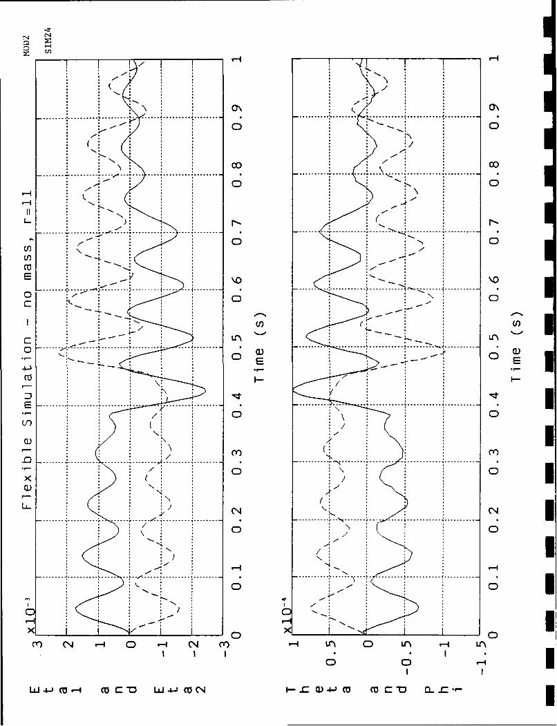
-ItI
.... ...I ... .. ..... ..... .I .. ....* - S
00: O0* :1
coo\ ** 0 \.~0
. ...... ... ...
-------.... .. .. .. . .. .. .. ---- -- -- - - - ----- ----
* 0 0,--- 4. * - . -
. .i .... .-.,.......... ... .... .. ... ... .. ....... . ......- . .....
E . .. .... ...... .............. I........ . .. .. ... ...-- - -- .- - -:.. . ... ... .........
,,- -- -,. , -.. ::
- - - ---- --........ I.
0 ,0t. J....*"..... . ........... .., .. :.:.
* S: CS - :
0 E0
X1:
m N 0. ...... " ..... . I ............
0 0
a. -W ccIqmCD WWM u- u C :' -
,,..5
',I
LL. ,2'
5- i <:.-~ <S-. .... ........ .... ..................... ".. . N...t ............ ......... .. .
* -.. ' 1, 0
Im I I~

CC
0
0
-0
CL) ---- 00- 0
0 0 0
L: '0 0 -

Lf)
0 0
0) -0 04- (I)
N.n
N.E E
0. 0 0 0000 0
0 0 0 0
o 0 I 0

t-4
cI~. 0
0
U) 0
CoC
0 '0-4-

\\0
cu cou
(N
(Nl C N cC C C~ CD C I-qL' ' '
0f -4-) L r
C C
C C
)Q
/ E -E
N- N
C---------------------------------C
(N Cr i1\ '-I 0 Cr U-q LnL
C. C- 0- C0
C CLD

.,0
FIT 1 '
............. ............... .| ............i .......... .i ..... .. ........... ...........
......................... \ ..[ .. . . . . . . . . . . . .. . . . . .-. . . . . ... . ..,. . . . . ..,. . . . . .
* * ' , ' i
.. .. .... .... ........ ... - -----------
V)I
.. ... .. .. --- -- -- --- -- --- ----....
....... ,, ... . ....-..... --- --- --
0
/o* .
* LC
... .. . . ....... :.. ......... . ...... . . ...........
W/
* ' \*) /<
E, /0-0" ' '- 0 0
C u i EW aC- "
I I

,--4
z I I 'IC
110 110
0 0
o 0
I
/toC 0
4
/
/
Co0
I / E FE
*- mi- (
o '/
C "./
0 /-) / "
/
0 /
N'
0 0
I I . .~ C I, I
'-4 0 0 '- I I
.fl (/ I-- C)

U) U
0 U).
Cr)D
W
E) 0
U) 0 0 0 0 1
>-0 L 0 0 0 IC
.9. 1
U')
a~) __
.0 /0-/ N.a.

N
Ci) i
0
~0
E
0
0
E00
0 00
E 0
0
(D0 0x
0 N () ON \ c m0 0 0 0 0 0 0 0 0
* 00 0 0 0 0 0 0 0 0 I
0 'DO 4-J

- I I I I I0
_0 0 0 0 0.. .. 0
_ 0 0 0 0) 0 1> - I I I IC3_ "0 0)4 _L
N' E
I/ ,i I
l o1
0 r- 0
0 ..

C31, -- 4'
o (N0
0
CD
N I-
LL-N
N N\00
'0 041

'D0
En 0
0
4-)
0
co -
00CE - ~ N N N NN N0
0
Co
0
0 0 0 0 0
0 0 0 0 0 0 0 0 0
0~C " 00 0 0-

-cLON
C 4 I..T 00 - L')h0 0
'1-'
0 0 0 0 • I •. . . 0 0 0,--
C 0 0- CL I--
Nf' N.N I
N0
Nr* Nn U.N r- U1U' )I
000 0 0
/ I I I
tI I I
//
0 0
U
0 0 0 0 -..
0 • 0 0 I
0 0t, I-.n

'D
01
0 0
-- - 0
C
U)uEE
4--
-4-i L 0 0
o 0'
(n /- o .
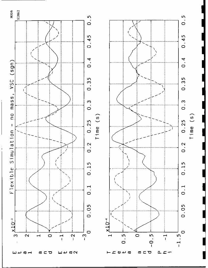
0Lr f
i ... I - o I o
....' ..-.-.- --------- --. --.t... . ... .. ...•
N 0C ................ .... .... . . .. . .......... ............ -----
' : " - -
: - u' ."""-.. 0 '
0/
........ .... . .... . ... .......... . ...........
* N ,* * a ai
00 0
,' -. ) a a- °, ,
a a .--- : -, ,m
r ) .......................... ............... ... ......................................
* " -- : - a " -
" --. .....I.. .. .. .. . ...... ... .. ....."
(r) \ a a ara
-------- ., .... ......... .... .......... ...... ... ..... ........ . . .. . .................... ......... ......................
E0 a a a 0• -a :
o: . I
.......... ........ ......... J-." .......... -------. .. ... .................... .... .
S a a "C
a\ a -aa a : /
" .E a a , UCEa a" a0a""
. . ... a/ .. . . . . . . . a . . . . . . . . . . . . .a . .. ..: a.. . . . . . . . . . . . " -" .. . . .. . . .
Q a0 a : a 0-. " '
l4-) a,- ' . *li- - a a a' a_ -

Lil WN
0 0
IfI
ca.EE
x /0
-C- 0 N 'R:T \0 CC) ;0 1 R N 0 N "
0 __ _ _ __ _ _ _ _0__ _
EI I I I
4 0 7
- -- -- -- - -- -
.. . ..... ... ... - .. .. ... ..
/ -0I II -
N) 0- - - - - - - - - - - - - - - -- E
0 00-

0
II -
NN
11E
LI)D
-0-
I-
X
10
0
0 0 0 0 0
0~ 00 0 0

4 -
m
NN
0
N (
-00
0 0E
000 1
L.LJ~~~~~ ~ ~ ~ ~ ~ 4- Or4 C D LJ4)C -C - U c)co a -

(YN
N
'N 'N C/)
NINC
(Y) E E
01
WE4
I-
0')-
Wca
N' N I- ' - l I f
0)0

,U1
0
OII
0) N
(00
(C1)L- 0
ao
0)0
0) 00
C) 0 0
00 0 0 0
0 0 I 0 0 04-0)

LI-
..... .... ..... ... . .. .... ...... C .... .... ............ . .......... . ... , ..........
- ---- - - - - . . ... . . .. - - - - - -- .. ..
),)-Y-'
-----...... ........ ........... •, .......... ..... ......... .......... ....... ,. c. ..- .. . . .......... .
(n.
I "".- " " E.. ._ ..-- ,
........ .... .... ................ ... ..... L .......
-5' ' 2 .
---. . .S , .. ' S, S - ,
*: , ... .5-
- ............................ ..................... " . . . . .
*r '5- (Y
-. 5
* i / \
.- ,
0 '0
-5 5 i' S* S
0 0
S 1 CO .I IWoa-
0o0C3 • 7
0 60C:

00C -
oIz u-0
U3 ' 0 4 CL
(0 U
-'
ot
C\ 0 Q0 0
CD 00

- -N
0
L.
0)00 ~ 0
C3 ' -

.. . ... . . .. .. .. . .... .. . . .. . .. .. .. ... .. .. .. .. ....... . ..co
cu cu
.,.-- ' ' '1
.: -.. -- - - - - - - -- -- -- -- - - - - - - - - - - - - - .. . .. . .. .. ........... ... .... ,,-- - -- -
.~~~~~~~~ ~ ~ ~ ................. .................... ....... .... ...... ... I ...........
1 .-
, , 0 0
0 0
0 0 1"
ui -W cu "i M C-k W .44WNc0- wi D Q
- S -. 5-. S , S
.. . ...... ..... . S .. ..... C .... .... 0>) '
I : "
'H * E
,,- *' N ' ,- ",,,. C .-o- o o o I(/ * S
0) • • N
0 0 -5-
t.* 11 - -S-": .J J 1I- r .- : 0. t --

zn - P
E0 0 0
a)) 0 004- LI
r*I-
LO
Cle,
C)
C %I
0 0 0 0 0
-0 F- M

CN
En~
0
WNN
co.
coN
0ErL N N j)CY I
0 - N m
0001~1
U '0 0 4-

- CN)
1 .1 (Y)Ct)
UNN
..... .
...... ......
CN
........ ... ................
CO
------ .......-- (n
a)L
a, I-i........ .. ....0. .. .....).. .......
co*
-, -. Lr
. ...... ..... N
N ~ 0 N ldt) U)U
I g 0 L0'-I 01