Fault Ride-Through Capability of Doubly-Fed Induction Generators Based Wind

Turbines

by

Abobkr Hamdia Abobkr

Submitted in partial fulfilment of the requirements

for the degree of Master of Applied Science

at

Dalhousie University

Halifax, Nova Scotia

March 2013

© Copyright by Abobkr Hamdia Abobkr, 2013

ii

DALHOUSIE UNIVERSITY

DEPARTMENT OF ELECTRICAL AND COMPUTER ENGINEERING

The undersigned hereby certify that they have read and recommend to the Faculty of

Graduate Studies for acceptance a thesis entitled “Fault Ride-Through Capability of

Doubly-Fed Induction Generators Based Wind Turbines” by Abobkr Hamida Abobkr in

partial fulfilment of the requirements for the degree of Master of Applied Science.

Dated: March 14,2013

Supervisor: _________________________________

Readers: _________________________________

_________________________________

iii

DALHOUSIE UNIVERSITY

DATE: March 14,2013

AUTHOR: Abobkr Hamida Abobkr

TITLE: Fault Ride-Through Capability of Doubly-Fed Induction Generators Based

Wind Turbines

DEPARTMENT OR SCHOOL: Department of Electrical and Computer Engineering

DEGREE: MASc CONVOCATION: May YEAR: 2013

Permission is herewith granted to Dalhousie University to circulate and to have copied

for non-commercial purposes, at its discretion, the above title upon the request of

individuals or institutions. I understand that my thesis will be electronically available to

the public.

The author reserves other publication rights, and neither the thesis nor extensive

extracts from it may be printed or otherwise reproduced without the author’s written

permission.

The author attests that permission has been obtained for the use of any copyrighted

material appearing in the thesis (other than the brief excerpts requiring only proper

acknowledgement in scholarly writing), and that all such use is clearly acknowledged.

_______________________________

Signature of Author

iv

TABLE OF CONTENTS

LIST OF TABLES ....................................................................................................... vii

LIST OF FIGURES ..................................................................................................... viii

ABSTRACT ................................................................................................................... xi

LIST OF ABBREVIATIONS AND SYMBOLS USED ............................................. xii

ACKNOWLEDGMENTS ............................................................................................. xv

Chapter 1 Introduction .................................................................................................... 1

1.1 Motivation ............................................................................................................ 1

1.2 Thesis Objective and Contribution ...................................................................... 4

1.3 Thesis Outline ...................................................................................................... 5

Chapter 2 Literature Review ........................................................................................... 6

2.1 Fault Ride Through Capability of DFIG Wind Turbines .................................... 6

2.1.1 Crowbar Technique .......................................................................................... 8

2.1.2 Various FRT Capability Techniques ............................................................. 10

2.2 Summary ............................................................................................................ 12

Chapter 3 Methodology ................................................................................................. 13

3.1 Introduction ........................................................................................................ 13

3.2 The Classic Configuration of a DFIG-Based Wind Turbine ............................. 13

3.3 Modeling of Wind Turbines ............................................................................... 14

3.3.1 Aerodynamic Component Model ................................................................... 15

3.3.1.1 Calculation of the Performance Coefficient ( ......................................... 17

v

3.3.2 The Mechanical Component Model ............................................................... 18

3.3.3 Wind Turbine Characteristics ........................................................................ 20

3.3.4 Model of DFIG System .................................................................................. 24

3.3.4.1 The Basic Concept of DFIG ................................................................................ 25

3.3.4.2 Reference Frame .............................................................................................. 28

3.3.5 Back-to-Back Voltage Source Converter ....................................................... 32

3.4 Doubly-Fed Induction Generator During Faults ................................................ 34

3.4.1 Reactive Power Support by DFIG ................................................................. 34

3.5 Modification of an RSC Controller .................................................................... 40

3.5.1 The New Proposed External Circuit .............................................................. 43

3.6 The STATCOM CONTROLLER. ..................................................................... 45

3.7 Summary ............................................................................................................ 48

Chapter 4 Results and Discussion ................................................................................. 50

4.1 Introduction ........................................................................................................ 50

4.2 Discretion of The System ................................................................................... 50

4.3 Case Study ......................................................................................................... 55

4.3.1 Case study 1: Voltage Support at Point B During Grid Faults ...................... 56

4.3.2 Case study 2: Voltage Support at PCC During Grid Faults ........................... 61

4.3.2.1 The Reactive Power Generated by DFIG During FRT ............................... 64

4.3.3 Case study 3: Evaluation of the Method ........................................................ 67

4.3.3.1 The Impact of Crowbar Activation During FRT ........................................... 67

4.3.3.2 The Impact of the Delta Reference Voltage ................................... 70

4.3.3.3 Comparison Between the External Circuit Method and Various FRT

Methods…… ................................................................................................................................... 71

4.4 Summary ............................................................................................................ 73

vi

Chapter 5 Conclusion and future work ......................................................................... 75

5.1 Conclusion ......................................................................................................... 75

5.2 Future Work ....................................................................................................... 76

REFERENCES .............................................................................................................. 77

APPENDIX A ............................................................................................................... 81

APPENDIX B ............................................................................................................... 83

vii

LIST OF TABLES

Table 4.1 Comparison between the voltage support of different types of faults .............. 57

Table 4.2 Comparison of voltage support during a fault with and without using the

external circuit.................................................................................................................... 63

Table 4.3 Comparison of PCC voltages between different cases of FRT to FRT with

crowbar .............................................................................................................................. 69

Table 4.4 Comparison of the voltage support obtained by the proposed method and the

method in [9] ...................................................................................................................... 72

viii

LIST OF FIGURES

Figure 1.1 The power generated (MW) from wind each year in Canada [2] ...................... 2

Figure 3.1 Classic wind turbine configuration with a doubly-fed induction generator ..... 14

Figure 3.2 Basic wind turbine components ........................................................................ 15

Figure 3.3 One-mass drive train representing the mechanical component ....................... 19

Figure 3.4 The performance coefficient Cp as a function of tip speed ratio λ, with pitch

angle β as a parameter ........................................................................................................ 20

Figure 3.5 Flowchart of the methodology of a wind turbine ............................................. 22

Figure 3.6 MATLAB/SIMULINK of a wind turbine with drive train .............................. 23

Figure 3.7 The wind turbine characteristics at β=0............................................................ 23

Figure 3.8 DFIG block with inputs and outputs ................................................................ 24

Figure 3.9 One-phase equivalent circuit for steady state of DFIG [30] ............................. 25

Figure 3.10 Active power flow of DFIG at different modes of operation according to

the slip sign ........................................................................................................................ 27

Figure 3.11 The dq model of DFIG ................................................................................... 29

Figure 3.12 The reactive power control as a function of the voltage at PCC in (E.On) .... 35

Figure 3.13 P-Q characteristics of a DFIG ........................................................................ 36

Figure 3.14 Characteristics of wind turbine voltage control [36] ...................................... 37

Figure 3.15 Voltage categories according to EN50160 ..................................................... 39

Figure 3.16 The depth voltage drop during a fault period [10].......................................... 40

Figure 3.17 Three controllers are represented in the RSC controller [9] ......................... 41

Figure 3.18 The electromagnetic torque and current controller........................................ 42

ix

Figure 3.19 The new proposed RSC controller ................................................................. 42

Figure 3.20 The proposed external circuit and current controller...................................... 44

Figure 3.21 The STATCOM controller ............................................................................. 45

Figure 3.22 The proposed external circuit applied to the STATCOM controller .............. 46

Figure 3.23 The proposed external circuit applied to the RSC and STATCOM

controllers .......................................................................................................................... 47

Figure 3.24 Voltage support at the point of common coupling by the DFIG and

STATCOM ........................................................................................................................ 48

Figure 4.1 The system’s one-line diagram ......................................................................... 51

Figure 4.2 Wind turbines with doubly-fed induction generator [40] ................................. 51

Figure 4.3 The three components of the RSC controller ................................................... 53

Figure 4.4 The MATLAB/Simulink model with the external circuit ................................ 54

Figure 4.5 The external circuit ........................................................................................... 54

Figure 4.6 Positive sequence voltages at point B during a one-phase grid fault .............. 57

Figure 4.7 The response of ΔVref during one-phase grid fault ........................................... 58

Figure 4.8 Positive sequence voltage at point B during a two-phase grid fault ................ 58

Figure 4.9 The response of ΔVref during two-phase grid fault ........................................... 59

Figure 4.10 Positive sequence voltage at point B during a three-phase grid fault ............. 59

Figure 4.11 The response of ΔVref during a one-phase grid fault ...................................... 60

Figure 4.12 Comparison of the voltage drop between the three types of faults ................ 60

Figure 4.13 Comparison of the voltage support between three different types of faults

when using the extenal circuit ............................................................................................ 61

Figure 4.14 PCC voltage using the external circuit during a one-phase grid fault ............ 62

x

Figure 4.15 PCC voltage using the external circuit during a two-phase grid fault ............ 62

Figure 4.16 PCC voltage using the external circuit voltage support during a three-phase

grid fault ............................................................................................................................. 63

Figure 4.17 Reactive power generated by DFIG at under-excited mode and during FRT

............................................................................................................................................ 65

Figure 4.18 Reactive power generated by DFIG over-excited mode and during FRT ..... 65

Figure 4.19 Average reactive power supplied during FRT for different modes of DFIG . 66

Figure 4.20 Reactive power generated by the DFIG at unity mode and during FRT ........ 67

Figure 4.21 Voltage at PCC using different methods of FRT for improvement ............... 69

Figure 4.22 The effect of deactivating the ............................................................. 70

Figure 4.23 Voltage at a DFIG terminal during a three-phase grid fault ........................... 71

xi

ABSTRACT

Due to growing concerns over climate change, more and more countries are looking to

renewable energy sources to generate electricity. Therefore, wind turbines are increasing

in popularity, along with doubly-fed induction machines (DFIGs) used in generation

mode. Current grids codes require DFIGs to provide voltage support during a grid fault.

The fault ride-through (FRT) capability of DFIGs is the focus of this thesis, in which

modifications to the DFIG controller have been proposed to improve the FRT capability.

The static synchronous compensator (STATCOM) controller has been applied with

proposed method to study its influence on the voltage at the point of common coupling

(PCC). The proposed method was also compared with other FRT capability improvement

methods, including the conventional crowbar method. The simulation of the dynamic

behaviour of DFIG-based wind turbines during grid fault is simulated using

MATLAB/Simulink. The results obtained clearly demonstrate the efficacy of the

proposed method.

xii

LIST OF ABBREVIATIONS AND SYMBOLS USED

List of Abbreviations

ASGs Adjustable speed generators

FSGs Fixed speed generators

DFIG Doubly fed induction generators

FRT Fault ride through

LVRT Low voltage ride through

E.On German grid code

UK National grid code

TSO Transmission system operator

DSO Disturbance system operator

SCIG Squirrel cage induction generator

EMF Electromotive force

RSC Rotor side converter

GSC Grid side converter

PCC Point of common coupling

VSC Voltage source converter

ESS Energy storage system

FACTS Flexible Ac transmissions system

UPFC United power flow controller

STATCOM Static synchronous compensation

PF The power factor

The voltage disturbance standard

xiii

List of symbols

The mechanical output power extracted from the wind

The performance coefficient

The tip speed ratio

The pitch angle

The air density

The area covered by the rotor blades

The wind speed

The turbine speed

The power gain

The electromagnetic torque

The mechanical torque

The total lumped inertia constant

The turbine rotor angular speed

The electrical power

The mechanical angular speed of the generator’s rotor

The electrical angular speed of the generator’s rotor

The stator voltage

The rotor voltage

The stator current

The rotor current

The stator resistance

The rotor resistance

The stator leakage inductance

The rotor leakage inductance

The mutual inductance

The stator induced

The rotor induced

The stator frequency

xiv

The rotor frequency

The number of the pole pairs of the generator

The slip

The electrical stator angular velocity

The electrical rotor angular velocity

d-axis stator voltage and current

q-axis stator voltage and current

d-axis rotor voltage and current

q-axis rotor voltage and current

d-axis stator flux linkage

d-axis rotor flux linkage

q-axis stator flux linkage

q-axis rotor flux linkage

The stator rotor active power

The generated active power

The stator rotor reactive power

d-axis reference rotor current

q-axis reference rotor current

The voltage at the point of common coupling

The reference voltage of DFIG

The measuring voltage at DFIG terminal

The slop or drop reactance

The reference voltage of the STATCOM controller

The measuring voltage at STATCOM terminal

The change of the reference voltage

The impedance type factor

The fault current

xv

ACKNOWLEDGMENTS

I thank God (ALLAH) for helping me in my research. I thank my lovely parents for

their asking Allah to help me. I thank my brothers and my sister and all my family who

pray for me, and I would thank my fiancee for her support ,and my friends here and back

home in my country Libya for their support. I thank my supervisor, Dr. Mohamed El-

Hawary for his guidance and advice.

1

CHAPTER 1 INTRODUCTION

1.1 MOTIVATION

Many of the world’s governments have now openly acknowledged that the use of

conventional energy sources is unsustainable due to environmental pollution and

dwindling resources. With this recognition comes the search for better ways to implement

alternative energy sources such as solar, hydroelectric and wind turbines. In addition to

causing less environmental degradation, these alternative sources have several

advantages. One advantage is that the prime mover’s input, which is later converted to

electricity, is renewable and thus will not run out. Moreover, there is an absence of waste

products such as carbon dioxide, which occurs in coal-fired power stations, and

renewable energy sources may require less maintenance than conventional sources.

Wind is by far the most popular renewable energy resources [1]. In 2012, a wind

turbine and wind farm database of more than 50 countries around the world was

published [2], showing the percentage of wind energy generated between 1997 and 2011,

inclusive. China was the largest user of wind energy, with power generated exceeding 60

GW. In Libya, wind power generated 20 MW, and Canada was ranked ninth as a wind

energy user, with a generation and production capacity of 5.265 GW. Figure 1.1 shows

Canada’s rise in wind energy production capacity from 1997 to the end of 2011.

2

Figure 1.1 The power generated (MW) from wind each year in Canada [2]

Wind energy was first used to generate electrical power in 1887 by Charles Brush in

Cleveland, USA. Brush used a DC generator with a battery to store the generated energy.

In 1951, using an induction motor as a generator was discovered, but it was not until the

1970s, when the price of gas skyrocketed, that they were given a wider acceptance. As

concerns over the environment grew through the 1980s and 1990s, so did the demand for

renewable, sustainable and ‘environmentally friendly’ energy sources. By the 21st

century, it was finally recognized that induction generators are among the best option to

fulfill these requirements [3].

In the past, a simple squirrel-cage-induction generator-based wind turbines were

directly connected to a three-phase power system and the rotor of the turbine was

connected to the shaft of the generator through a fixed gear box. However, this type of

0

1000

2000

3000

4000

5000

6000

Cap

acit

y(M

W)

Year

3

generator had to operate at a fixed wind speed, which is impractical and considered a

disadvantage. In response to this limitation, some induction generators were developed to

use pole-adjustable winding configurations in order to operate at variable wind speeds.

Nowadays, many modern and large wind turbines use adjustable-speed generators

(ASGs). Their main advantages over fixed-speed generators (FSGs) are that mechanical

stress is reduced, power quality is improved, and system efficiency is higher. The most

common type of ASGs used to produce electricity in wind turbines is the doubly-fed

induction generator (DFIG) [4].

The most important advantages of using DFIGs coupled to wind turbines are:

They provide a steady output voltage, including amplitude and frequency, regardless

of wind speed and can thus be directly connected to the grid.

The mechanical load stresses on wind turbines, which are produced during wind

gusts, are reduced when using DFIGs. Additionally, during periods of low wind

speeds, a DFIG maximizes the extracted energy (for details, see [4]).

The possibility for independent control of active and reactive power due to smooth

integration of wind turbine into the grid is achieved [5].

Because only 25% to 30% of the power exchanged between a DFIG and the grid is

completed through the power converter, the size of the power converter when using a

DFIG is around one-quarter of the size of the power converter when three-phase

synchronous generators are used. Thus, DFIGs lower the cost of the power converter

[6].

The behaviour of DFIGs during grid disturbances like short-circuit faults has been the

focus of numerous studies. In the past, the majority of national network operators did not

4

require that wind farms be connected to the grid during grid disturbances. However, due

to an increase in wind farms, it is now mandatory for wind turbines to be connected to the

grid during disturbances, in order to support it with reactive power [7]. Fault ride through

(FRT) or low voltage ride through (LVRT) along with other methods and techniques have

been developed to improve the FRT capability of DFIGs during fault periods.

1.2 THESIS OBJECTIVE AND CONTRIBUTION

As mentioned, numerous methods have been applied with the aim of improving the

FRT capability of DFIGs. Examples include crowbar protection and reactive power

sources in general. However, and as will be detailed in the next chapter, these methods

have drawbacks. The key objective of this thesis is therefore to enhance the FRT

associated with DFIGs during fault periods, improving the FRT requirement of voltage

support during grid disturbances by reducing the voltage drop peak during fault periods.

To this end, an external control circuit is proposed and applied to enhance FRT capability.

Results obtained when using the proposed method will be compared to results obtained

without this method as well as with those obtained by other techniques, including the

crowbar method.

The idea for this work was derived from three theories. First, DFIG control is the key

to DFIG performance during faults [8]. Second, the rotor side converter (RSC) controller

can be modified to support grid voltage and, as a result, improve the FRT [9]. And third,

the drop voltage is a function of a fault current [10]. These key theories will be discussed

in detail later in this thesis.

The major contribution of this research work is proposing an improved FRT capability

by modifying the RSC controller of the DFIG. The RSC controller is modified by

5

applying the external circuit so that the DFIG is able to support the grid voltage during

grid fault and recovery.

With the intent of improving the FRT capability of DFIGs, a model of a wind turbine

and drive train are presented and dynamic equation models of DFIGs are discussed and

demonstrated.

1.3 THESIS OUTLINE

This thesis is organized in five chapters. The first chapter introduces the motivation

behind this thesis as well as its objective and contributions. The second chapter reviews

the literature and research area covered by this thesis. The third chapter discusses

modeling of wind turbines and DFIGs and the behaviour of DFIG-based wind farms with

AC grid connection during grid fault. This chapter also discusses some drawbacks of a

specific method frequently used to improve the FRT capability of DFIG. Subsequently,

this chapter explains the methodology and theory of this thesis and presents information

on the origin of this method. In Chapter 4, the proposed method is applied to a DFIG-

based wind turbine with power transmission system to check the validity of the presented

method with regards to improving the FRT. Results obtained from the current research

work are also compared to those obtained from other works. The final chapter provides

the conclusion and some ideas for future work.

6

CHAPTER 2 LITERATURE REVIEW

This chapter briefly presents a literature review of the FRT capability of DFIG and the

various methods that have been used, with varying success, to enhance the FRT issue.

2.1 FAULT RIDE THROUGH CAPABILITY OF DFIG WIND TURBINES

Fault ride through (FRT) or low voltage ride through (LVRT) can be defined as

procedure may happen for an electric device or, in our case, a DFIG. Below are a few

scenarios describing what should happen to an electric device during and after a voltage

drop resulting from a load disturbance or other fault.

The device should be disconnected from the AC grid temporarily until the dip

disappears, after which the device should be reconnected.

The device should never be disconnected from the grid and should remain constantly

operational.

The device should stay connected and act as a reactive power source to support the

grid voltage.

Around the world, network operators issue grid codes, such as the German grid code

(E.On) and the national grid code (UK). These grid codes determine which operational

behaviour should occur or what action should be taken. Currently, according to the

German grid code, wind turbines during a fault period (e.g., a short-circuit fault) must

supply voltage support or reactive power support by increasing the provided reactive

current to the grid [11]. In this case, implementation of the last of the three scenarios

listed above is required.

7

As early wind turbines, some of which were coupled to a squirrel cage asynchronous

machine, were very sensitive, the protection system disconnected the turbines even during

minor disturbances. Nowadays, however, it should be a goal that wind turbines have the

ability to continue operational through a fault and remain connected to the power system

at all times [10].

Research indicates that the two most effective factors determining the FRT capability

of DFIG wind turbines are converter control and converter protection system [8]. These

two factors influence the performance of DFIGs during normal operation as well.

Nevertheless, in [8], there is no information regarding voltage support recovery during a

grid fault. During such an incidence, the voltage at the DFIG terminal dips down, causing

a high transient rotor current due to the physical component of DFIG (namely, the

magnetic coupling between the stator and the rotor, according to flux laws). Hence,

during grid disturbances, stator disturbances are transmitted to the rotor [8].

To protect the rotor winding of DFIG and its converter circuits, a rotor over current

protection called crowbar is applied [12] . The crowbar provides a safe route for the high

transient rotor current by short circuiting the generator rotor windings, switching the

crowbar to protect the rotor side converter (RSC) during faults.

Several principles and guidelines should be considered in designing crowbar

protection [10]. Below are four key principles:

First, keep the wind turbine connected.

Second, prevent consumption of active power during a fault.

Third, support the grid with reactive power during a fault and assist in voltage

recovery.

8

Fourth, enable a return to normal operation and steady-state condition quickly and

efficiently.

From the principles listed above, we can conclude that the crowbar technique is a

useful way to solve FRT capability. Not surprisingly, the crowbar method is considered

the most popular of conventional techniques to improve the FRT capability of DFIG.

2.1.1 Crowbar Technique

In [13], a crowbar protection was applied using diodes and a thyristor in a series with a

resistor. In [8], it was noted that FRT capability can be improved by using a proper value

of crowbar resistance. Furthermore, to damp the torsional oscillation in the drive train

caused by grid sag, a damping controller was applied to a thyristor crowbar.

A disadvantage of the crowbar protection method was presented in [14], where it was

shown that, during a fault event, the controllability of a DFIG during the firing of the

crowbar is lost because the DFIG will behave as a conventional squirrel cage induction

generator (SCIG). Another drawback in using the crowbar method is stated in [15]. Since

the stator during grid fault absorbs reactive power instead of supplying reactive power to

the power network, two proposed methods have been implemented to prevent reactive

power from being consumed. The aim of these two methods is derived from the principle

of the theory of activation crowbar. The first method is to reduce the voltage value that

operates the crowbar. To do this, an optimum value of a DC-chopper resistor is

employed. In the second method, a strategy involving a grid side converter (GSC)

controller is designed so that the main priority of GSC control is to compensate for the

stator reactive power as well as support grid voltage recovery.

9

In contrast to conventional crowbar techniques, a fully controllable crowbar protection

method was implemented in [16] to improve the FRT capability of the DFIG. It was

controlled by the DC-link voltage. Another disadvantage of the crowbar method is that

when the crowbar turns off and then, due to high rotor current or high voltage of the DC-

link, attempts to turn back on, a two-phase fault can occur. This kind of fault causes a

high negative-sequence voltage component in the stator winding, leading to a high rotor

slip and inducing a high rotor voltage in the rotor winding. Consequently, the rotor

current becomes difficult to control during this event until the fault has been cleared.

To solve the difficulties of controlling the rotor current, a new control method of the

RSC, instead of using the crowbar method, was presented in [17]. However, some

difficulties arose due to electromotive force (EMF) induced in the rotor that depended on

negative-sequence voltage components in the stator-flux linkage and the rotor speed. The

idea was based on eliminating undesired components in the stator-flux linkage by

injecting the opposite components in the rotor current, with the intent to constrain the

rotor current supplied to the RSC. This method, however, had limitations related to the

control objective.

The differences between FRT with activated crowbar and with deactivated crowbar

were introduced in [11]. According to the authors , the main disadvantage of using

crowbar was the limitation of the reactive current provided from the DFIG during grid

disturbances, which led to a limitation of voltage recovery support. Furthermore, the

controllability of the DFIG during crowbar firing was lost because the DFIG will behave

as a conventional squirrel cage induction generator.

10

2.1.2 Various FRT Capability Techniques

A protection scheme to enhance FRT capability was presented in [18]. In this work,

instead of using the crowbar protection method during a fault condition, a supplementary

dynamic resistor in a series with the RSC was applied. The advantages of using this

method are reducing the disability time of RSC and reducing the torque fluctuation during

protection time.

In [19] another technique aimed at improving the FRT capability of DFIGs without

using the crowbar method, a scheme was proposed that uses a stator side series connected

braking resistor, a DC-link chopper, and a coordinated control strategy of the DFIG. This

scheme was designed to enable the RSC to remain connected during faults. As a result,

the controllability during faults was maintained and the reactive power to support grid

voltage recovery during grid faults was achieved. Moreover, by not using the crowbar

protection option, stress on the turbine mechanical systems and specifically the torque

fluctuation was significantly reduced. However, it was reported that the cost of using this

scheme is high compared to the crowbar method. Other techniques can be applied to

improving the FRT capability of DFIGs by connecting various reactive sources at specific

locations.

In [11], shunt reactors and a capacitor were coupled to the best location, defined here

as the point of common coupling (PCC), to generate the grid reactive power needed.

Another location for connected reactive power sources to improve FRT capability is at

the DFIG terminal, as proposed in [20]. In this research, it was applied by connecting an

additional series-connected voltage source converter (VSC). Results obtained from this

method demonstrated improved FRT capability compared to existing applied methods,

11

including the crowbar protection method. However, the method is considered more

complicated, as it requires the use of three VSCs.

In [21], a comparison of different FRT solutions – namely, energy storage system

(ESS) methods, the flux method and the crowbar method – was presented. The

comparison evaluated the effects of the three different methods of FRT solutions under

balanced and unbalanced faults, depending on wind turbine response. The results

obtained demonstrated that, with the ESS method, it is not necessary to use the crowbar

method, as the generator and converter continue to be connected and support the grid

faults. However, this requires oversizing the RSC to hold out the high rotor current.

Furthermore, the flux method was difficult to control, which can be observed from the

oscillation at the voltage recovery. In contrast, the crowbar method provides operational

stability, as can be noticed from the small transient at voltage recovery and the limitation

of the rotor current obtained.

Kazi and Jayashri [9] proposed what seems to be a unique dynamic controller of

solving and enhancing the FRT capability of DFIGs. A new modification of the RSC was

applied by combining electromagnetic torque, current and voltage controller.

Furthermore, the research modeled a flexible AC transmissions system (FACTS), one of

the most widely used reactive power sources. Here, FACTS was used to generate and

observe the reactive power required at the PCC. Subsequently, the proposed FACTS

controller with FRT capability was compared to FRT capability with crowbar controller.

It was reported that, when using the crowbar method, undesirable fluctuations of

electromagnetic torque most likely occur. To solve this problem, FACTS was applied.

12

In [22], a novel scheme is proposed to help DFIGs remain connected to the power

system and support voltage to the grid during unbalanced voltage or faults to assist

voltage recovery. The concept of the research is that three single-phase converters can be

used as an alternative to one three-phase converter.

2.2 SUMMARY

This chapter discussed various options for improving the FRT capability of DFIGs in

order to stay connected to the power system network during fault conditions. As we saw,

the most common method used is crowbar, but this method was revealed to have

disadvantages such as loss of the controllability of DFIGs and their overconsumption of

reactive power during grid faults. Consequently, the literature review presented some

alternative methods to using the crowbar, citing their advantages and limitations. A few

of these alternatives are using a resistor with RSC and connecting reactors and capacitors

at the PCC.

13

CHAPTER 3 METHODOLOGY

3.1 INTRODUCTION

This chapter presents the methodology used to improve the FRT capability of DFIGs

during faults. Specifically, it introduces the modification of the RSC of DFIGs by

applying the proposed external circuit in order to enhance the FRT issue. In the next

section, a classic configuration of a DFIG-based wind turbine is discussed prior to

introducing the external circuit method.

3.2 THE CLASSIC CONFIGURATION OF A DFIG-BASED WIND TURBINE

In most instances, generating electricity from wind turbines is a two-stage process. In

the first stage, the turbine rotor (prime mover) converts kinetic energy from the wind into

mechanical rotational power. In the second stage, a generator converts mechanical power

into electrical power. There are presently two options for coupling a turbine rotor to a

generator shaft. One option, which is the most popular, involves coupling the two

components physically via a gearbox. The other option is to connect the rotor directly to

the generator. In the case considered, the type of generator is a DFIG, where the stator is

directly connected to the grid and the rotor winding is connected to the grid via a back-to-

back voltage source converter (BVSC). A common configuration of a DFIG-based wind

turbine is illustrated in Figure 3.1. In the next section, a model of a wind turbine is

introduced.

14

Figure 3.1 Conventional wind turbine configuration with a doubly-fed induction

generator

3.3 MODELING OF WIND TURBINES

In modelling wind turbines, three basic components are taken into consideration: the

turbine rotor, the gear box, and the generator shaft and electrical generator. These are

defined as aerodynamic, mechanical and electrical components, respectively. The

interaction between these three components is shown in Figure 3.2. In [23], it was

determined that the amount of mechanical power that can be extracted from the wind by a

turbine rotor depends on the dynamics of the wind (the aerodynamic component) and the

response of wind turbine (the mechanical component). Hence, both the aerodynamic

model and the mechanical model are required in wind turbine modeling.

Blades of wind

turbine

Gear boxDFIG

AC/DC/AC

Back to Back Voltage Source Converter

Transformer

Load

Line

Impedance

Grid equivalent

reactance

Grid

Rotor

GSC RSC

B1B2

15

Figure 3.2 Basic wind turbine components

3.3.1 Aerodynamic Component Model

In a wind turbine simulation with FRT capability, it is desirable to involve the

aerodynamic model during grid disturbances [12]. The aim of this model is to extract

mechanical power from the wind by the rotor of the wind turbine, as mentioned in section

3.2. Equation ( 3-1) is referred to as a mechanical power equation [24, 25]. The

magnitude of this equation depends on air density and wind velocity [1].

( 3-1)

where:

: the mechanical output power extracted from the wind, W

: the performance coefficient or the power coefficient

λ : the tip speed ratio between turbine speed and wind

Wind turbine

rotor

Wind turbine shaft

Gear box

Generator shaft

Generator

Mechanical component Aerodynamic

component

Electrical

component

Wind

16

speed, ⁄

: the pitch angle of the rotor blades, deg

: the air density, Kg/m3

: the area covered by rotor blades, m2

: the wind speed, m/s

To simplify the computations, Equation ( 3-1) can be rewritten in the per unit system

and calculated for specific values of and , using a power gain constant, as follows:

[26]:

(3-2)

where:

: the power extracted from the wind in (pu) for the base

power of specific values of and

: the performance coefficient of the maximum value of ,

in (pu), so that ⁄

: power gain

: the wind speed in pu, so that

⁄

The performance coefficient or the power coefficient is considered as a

characteristic of wind turbines. However, there are various methods to calculate [12].

The next subsection presents these methods.

17

3.3.1.1 Calculation of the Performance Coefficient (

The performance coefficient is a function of the tip speed ratio λ and the pitch

angle of the rotor blades . During this research, three different methods were found [12,

24, 27].

1. Blade element method: in using this method, the calculation of is

considered difficult and complicated [27].

2. Look-up table method: the calculation of is done using curves relating

versus , while is a parameter.

3. Numerical approximations method: the relationship defining is nonlinear;

therefore, the numerical approximation is a perfect option to calculate . This

approximation has been improved in [24, 26], as follows:

(

)

(3-3)

where:

(3-4)

The third method was employed in this thesis. Furthermore, by using Equations (3-3)

and (3-4), the characteristics of wind turbines can be determined as will be explained

later.

18

3.3.2 The Mechanical Component Model

The alternative name of the mechanical component model most widely used is a wind

turbine rotor-generator drive train model [23]. The drive train consists of:

wind turbine (WT) shaft

gearbox

generator shaft

The drive train model can be represented either by a two-mass or a one-mass system

model [28]. If the one-mass model is utilized, the WT, gearbox and generator are lumped

together into one equivalent mass. The following equation is known as the mechanical

swing or motion equation. This equation models the drive train [29].

( 3-5)

where:

: the electromagnetic torque

: the mechanical torque

: the total lumped inertia constant

: the turbine rotor angular speed

: the electrical power

: the mechanical angular speed of the generator

19

Accordingly, and with [12, 30], Figure 3.2 has been expanded and developed into

Figure 3.3, as follows.

Figure 3.3 One-mass drive train representing the mechanical component

Figure 3.3 shows the three wind turbine components. Once the is calculated

from the aerodynamic model, it will be fed to the drive train model. The objective of the

drive train model is to calculate the , after which it is converted to by using

the gear box ratio and subsequently delivers the to the generator. In the next

section, an example of applying the aerodynamic and mechanical component equations in

order to investigate the characteristics of a specific wind turbine is presented.

Aerodynamic model

Wind

Power Gear box

ratio

KEquation

(3-2),(3-3)&

(3-4)

Induction

GeneratorGear box

Generator shaftWind turbine rotor

Drive train model

To Grid

20

3.3.3 Wind Turbine Characteristics

The characteristics of any wind turbine may be defined as , as a function of

WT- rotor speed for different wind speeds as well as different pitch angles, .

Equations (3-2)(3-3)(3-4) are used for this purpose. A MATLAB program was written to

draw the performance coefficient ) as a function of tip speed ratio ( ), with pitch angle

( as a parameter. As a result, the (base) and (base) at have been calculated as

0.4798 and 8, respectively, as shown in Figure 3.4.

Figure 3.4 The performance coefficient Cp as a function of tip speed ratio λ, with pitch

angle β as a parameter

Once the (base) and (base) are calculated, they will be applied to the aerodynamic

and mechanical models to find the relationship between VS . It is

2 4 6 8 10 12 14-0.1

0

0.1

0.2

0.3

0.4

0.5

0.6

Tip speed ratio lmbdas

Perf

orm

an

ce c

oeff

icie

nt

cp

performance coefficient cp as a function of tip speed ratio with pitch angle as a parameter

0 deg

2 deg

5 deg

10 deg

15 deg

20 deg

X: 8

Y: 0.4798

21

should be noted that the WT rotor speed is referred to the generator side [1, 26], so

that:

(referred to as the generator)

( 3-6)

where:

: the base of the mechanical angular generator speed

(constant) ,

In this thesis, and unlike the conventional simulations which use the wind turbine

block in the MATLAB /SIMULINK library, a block was modeled by supplementing the

drive train subsystem with assumption of 0.8 pu and =3.5. In this example,

12(m/s) base wind speed, at this base wind speed 0.73 pu, and =1.2

(pu) have been implemented using MATLAB /SIMULINK. These values have been taken

from [26], for the wind speeds 14, 13.2, 12, 10.8, 9.6, 8.4, 7.2 and 6 m/s. The MATLAB

program illustrated in Figure 3.4 is given in Appendix A, while the wind turbine

characteristics methodology is summarized in the flowchart Figure 3.5, the Simulink file

is shown in Figure 3.6, and the wind turbine characteristics are illustrated in Figure 3.7.

The aim of the characteristics of any wind turbine is to provide an expectation of how

to design the generator’s control system in order to track these characteristics and extract

maximum power from the wind.

22

Figure 3.5 Flowchart of the methodology of a wind turbine

β

( )

Wind speed

Wind speed ( )=Wind speed / Wind speed base

referred to G ( wind speed ( )

at β =0

at β =0

MATLAB program

to calculate λ base

and base as

figure (3-4 shows

calculation

referred to

generator

Wind turbine

characteristics as figure

(3-7) shows

Drive train model Generator

Gear

box

ratio

Wind speed (

referred to G ( )

( )

β

23

Figure 3.6 MATLAB/SIMULINK of a wind turbine with drive train

Figure 3.7 The wind turbine characteristics at β=0

0.3 0.4 0.5 0.6 0.7 0.8 0.9 1 1.1 1.2 1.3-0.2

0

0.2

0.4

0.6

0.8

1

1.2

1.4

Turbine speed referred to generotor side (pu)

Mec

han

ical

po

wer

(p

u)

Wind turbine characteristics ( pitch angle =0 deg)

7.2 m/s

6 m/s

8.4 m/s

9.6 m/s

10.8 m/s

12 m/s

13.2 m/s

14.4 m/s

24

3.3.4 Model of DFIG System

Double-fed induction generators are preferable in wind turbine applications that

require a constant output power system frequency at various speeds of the generator shaft.

DFIGs are electric generators that have windings on both stator and rotor sides. The stator

is directly connected to the grid and the rotor is connected to the grid via a power

converter, as shown in Figure 3.1. Furthermore, the voltage on the stator is supplied from

the power system and the voltage on the rotor is induced by the power converter, the

generated electrical power is supplied to the grid through both the stator and the rotor.

The DFIG has three inputs: the stator voltage , the rotor voltage , and the

mechanical angular speed of the generator’s rotor ( . It also has three outputs: the

induced stator , the rotor currents , and the electromagnetic torque , as

shown in Figure 3.8. The next sections provide a brief description of DFIG theory and

equations.

Figure 3.8 DFIG block with inputs and outputs

stator

rotor

DFIG

25

3.3.4.1 The Basic Concept of DFIG

As illustrated in Figure 3.8, when the stator is supplied by the grid voltage of

frequency , the stator flux is induced and will rotate at a constant speed, which is known

as synchronous speed . Consequently, and according to Faraday’s law, the stator flux

will induce an electromotive force in the rotor windings ( ). This, together with the

injected voltage from the power converter to the rotor windings , will induce the rotor

current, , which also produces a rotating rotor flux. Similarly, this rotating rotor flux

will induce the electromotive force in the stator windings ( ), which induces a

current in the stator windings, . The equivalent circuit for steady state of DFIG is

illustrated in Figure 3.9.

Figure 3.9 One-phase equivalent circuit for steady state of DFIG [30]

Where:

: the stator, rotor resistance

: the stator, rotor leakage inductance

: the mutual inductance

: the stator, rotor-induced current

26

: the stator, rotor electromotive force induced

The voltages and currents in the rotor windings rotate at a speed which is known as

the electrical rotor angular velocity ). Likewise, the voltages and currents in the stator

windings rotate at the electrical stator angular velocity ( ). The relation between and

is given as follows:

( 3-7)

where:

: the electrical angular speed of the generator’s rotor

: the number of the generator’s pole pairs

In addition, the relation between and is commonly called the slip (s). By

combining this relation with Equation (3-8), the relation between and is expressed

in Equation ( 3-9)

(3-8)

( 3-9)

Where

the stator, rotor frequency

27

The sign of the slip determines the mode of the DFIG operation, either in a sub-

synchronous operation or hyper-synchronous operation, as well as the receiving or

supplying the power, as shown in Figure 3.10.

Figure 3.10 Active power flow of DFIG at different modes of operation according to

the slip sign

According to various models of DFIGs established by numerous authors, the space

vectors of the machine are represented by different reference frames in order to create a

dynamic model of a DFIG. Examples of these frames are the stator reference frame

, the rotor reference frame , and the synchronous reference frame . It

should be noted that the difference between these reference frames is the rotating speed of

the frame, where the speeds are zero (stationary), the electrical angular speed of the

generator’s rotor ( and synchronous ( of the given frames respectively.

To achieve an independent control of the active and reactive power and to simplify the

model of DFIG by eliminating the zero sequence components, the direct and quadrature

rotating axis reference frame has been frequently implemented to model the DFIG.

(A) Sub-synchronis operation(B) hyber-synchronis operation

28

3.3.4.2 Reference Frame

Over the course of researching this thesis, many studies aimed at modeling the DFIG

in reference were analyzed [7, 27-33]. The main difference between the models were

the signs. Some were modeled as a general machine (the signs of the currents and are

identical and indicate that the currents flow toward the machine), unlike Figure 3.9 [31-

33], while other models were designed as a generator (the signs of the and are

opposite, where flows toward the grid) [7, 28] or established as a generator (the signs

of the and are similar, where and flow toward the grid), as shown in Figure 3.8

[27, 29]. However, even between [29] and [27] there is a difference, but not in the current

signs. Instead, the difference is in the polarity of the voltage, which is induced by a

changing flux. Therefore, to find an acceptable model of a DFIG, mathematical and

electrical laws have been applied.

First, a stator and rotor flux linkage ( will be produced by the stator and rotor

induced currents , respectively. By a change in the flux linkage, the polarity of

the induced voltage opposes the current which produces it (Lenz’s law).

Second, a transformation matrix is applied to the traditional a, b, c model to switch to

the reference frame. As a result, Figure 3.9 will be devolved to Figure 3.11.

Furthermore, from Figure 3.11, it can be observed that, the polarities of the induced

and voltages which are induced by the change of the flux linkage

and

will oppose the polarities of the and , respectively .

29

Figure 3.11 The dq model of DFIG

Third, applying the Kirchhoff voltage law to Figure 3.11 will give:

( 3-10)

Fourth, applying the pharos notation theory to simplify, the reference frame can by

expressed as follows:

[

]

( 3-11)

Hence:

( 3-12)

30

[

]

In a similar way, in

[

] (3-13)

By substituting Equations (3-8) ( 3-12) and (3-13) into ( 3-10), the stator and rotor

phase of DFIG in the reference frame can be expressed according to the following

equations:

( 3-14)

( 3-15)

where:

( 3-16)

31

where:

d-axis stator voltage and current

q-axis stator voltage and current

d-axis rotor voltage and current

q-axis rotor voltage and current

d-axis stator flux linkage

d-axis rotor flux linkage

q-axis stator flux linkage

q-axis rotor flux linkage

It should be noted that Equations ( 3-14), ( 3-15) and ( 3-5) represent the DFIG as a fifth-

order model. Also, DFIG can be represented as a third-order model when the stator

transients (i.e., the differential term in Equations ( 3-14)) are left out, which increases the

computation speed in power system simulation software [27, 32]. In [34], a first-order

model was given by leaving out the rotor transient. It should also be mentioned that the

demonstrated equation of the DFIG dynamic model ( 3-14)( 3-15) are also given in [29].

The active power of the stator , rotor , generated power and

electromagnetic torque are calculated as:

32

( )

( )

(3-17)

The reactive power of the stator , rotor and generated power are

calculated as:

( )

( )

( 3-18)

3.3.5 Back-to-Back Voltage Source Converter

As mentioned earlier in this chapter, the stator and rotor circuits have different

frequencies. In general, the stator frequency ) is fixed if the stator is connected directly

to the grid, which means that the is fixed. In contrast, the will supply via the voltage

source converter, which allows for a modification of the . Hence, the rotor

frequency ) is variable and depends on the , according to Equations (3-8) ( 3-9).

This injected rotor voltage (which means must be at an appropriate value so that

is equal to its reference value, allowing the DFIG to extract the maximum amount

of from the wind turbine.

33

In general, it is possible to conclude that a relation between and the power

generated by DFIG exists. In fact, a relation between and the generated stator power

and is present. In other words, the is controlled and traces its reference value to

achieve the optimum value of the and . Furthermore, by applying a reference

frame in a specific way, the stator’s active and reactive power can be controlled

independently so that control the and , respectively.

As is known, there are a many of different types of controllers. The one most

extensively used is the proportional-integral (PI) controller. It is possible to insert the

input of (PI) as a current while the output of (PI) as a voltage by means of using the

proper proportional-integral parameters of (PI). Moreover, the relation between the

current and the voltage is transformed to transfer function using Laplace domain [35].

This controller is called the rotor-side converter (RSC) control. Once the reference rotor

currents are calculated and inserted into the PI controller, the voltages

are obtained. These will be injected into the DFIG via the rotor-side converter

(RSC).

The other part of the two-level converter (AC/DC/AC) is known as the grid-side

converter (GSC). A DC-link separates the RSC and GSC, as shown in Figure 3.1. The

aim of the GSC is to maintain the DC-link voltage as a constant. It is noteworthy to

mention that the major part of the clarification presented in sections 3.3.4 and 3.3.5 are

derived from [10].

34

3.4 DOUBLY-FED INDUCTION GENERATOR DURING FAULTS

In the past, the majority of grid operators did not require that wind farms be connected

to the grid during grid faults. However, at present, due to an increase in the

implementation of wind turbines, keeping wind turbines connected during grid faults has

become mandatory. Moreover, during grid faults, wind turbines have to supply voltage

support or reactive support. These two requirements are called fault-ride through (FRT).

3.4.1 Reactive Power Support by DFIG

Reactive power or voltage support is requested during grid faults by increasing the

reactive current provided to the grid in order to support the grid voltage.

Reactive power control (supply or consumption) as a function of the voltage at the

point of common coupling between the DFIG and the grid (PCC) is defined in grid codes,

which are issued by the transition system operators (TSOs). It should be noted that, due to

the difference between grid structures, the definition may vary from company to

company. For instance, Figure 3.12 shows the relation between the reactive power control

of DFIG and the voltage at PCC in a German grid code [11].

From Figure 3.12, it can be concluded that, when the voltage at the PCC decreases

below a specific range, the DFIG would act as a reactive power source (e.g., as

capacitive) and supply reactive power to the grid in order to increase the voltage.

Furthermore, the DFIG would turn into over-excited mode. On the other hand, if the

voltage at the PCC increases to a level above a specific range, the DFIG would act as an

inductive load and consume reactive power in order to decreases the voltage. In this case,

the DFIG would operate in under-excited mode, as illustrated in Figure 3.12 [10].

35

Figure 3.12 The reactive power control as a function of the voltage at PCC in (E.On)

Commonly, the reactive power sign depends on DFIG conditions. So, if the DFIG is in

over-excited mode, the reactive power is labelled positive. Conversely, if the DFIG is

in under-excited mode, the reactive power is labelled negative. The (P-Q)

characteristics of a DFIG are shown in Figure 3.13.

1

Volt

age

at P

CC

(pu

)1.16

1.1

1

0.92

0.95 0.95 0.925

Power factor

Over-excited

Capacitive

Leading

Supply(Q)

Under –excited

Inductive

Lagging

Consume (Q)

36

Figure 3.13 P-Q characteristics of a DFIG

According to [11] and Figure 3.13, three advantages of a DFIG as a reactive power

source can be concluded as follows:

Firstly, the DFIG can provide reactive power even though no active power is

generated.

Secondly, the DFIG can supply more reactive power in under-excited mode than in

over-excited mode.

Thirdly, the DFIG has the ability to operate at all four quadrants of the complex plan.

Consequently, the DFIG becomes a preferable reactive power source for the

grid requirements, especially during faults.

Therefore, during grid faults, the DFIG can supply reactive power during transient

situations, including faults. This is the key focus of the present thesis and will be

discussed in the next section.

37

Even more specifically, DFIG-based wind turbines have to support the grid voltage by

injecting additional reactive current. For this purpose, the voltage control must be

stimulated (as shown in Figure 3.14) so that during faults and when the voltage dips more

than 10%, the voltage control can supply reactive current within 20 (ms) after the fault is

realized. Subsequently, for each 1% of the voltage dip, at least 2% of the rated reactive

current is supplied. For instance, it should supply at least 0.5 reactive current any

time the voltage dips under 25% due to grid disturbances or when the dead band around

the rated voltage of 10% is allowed, as illustrated in

Figure 3.14 [36].

In addition, grid codes nowadays demand a standard for successful FRT of wind

turbines, requesting that voltage support be at least up to 15% rating voltage [14].

Figure 3.14 Characteristics of wind turbine voltage control [36]

Dead band

around reference voltage

Voltage

Additional reactive

current

Voltage limitation

(under-excited mode)

Voltage support (over-

excited mode)

reactive current

rated current

rated voltage

drop voltage during fault

38

In general, only 30% of power is exchanged through the power converter between the

DFIG and the grid. Consequently, the required size of the converter is only about 30% of

the full-power converter, and thus DFIGs are considered as non-full-power converters [6].

In fact, non-full-power converters such as DFIGs are more sensitive to grid faults than

full-power converters and therefore require protection. Over-current protection, called

crowbar protection, is commonly used [8]. As mentioned in Chapter 2, crowbar

protection is considered an FRT capability method and has many disadvantages, as

summarized below:

1. During faults and crowbar activation, the controllability of DFIG is lost because the

DFIG would behave as a squirrel cage induction generator [14].

2. During faults and crowbar activation, the stator of DFIG observes reactive power

instead of providing reactive power and voltage support to the grid [15].

3. Due to the high sensitivity of a crowbar to any case of a high rotor current or a high

voltage of the DC-link, repeatedly turning the crowbar circuit on and off causes a high

negative voltage component in the stator. This in turn causes a high rotor slip, which

induces a high rotor voltage in the rotor. Consequently, the controllability of the rotor

current during this event becomes difficult [16].

4. During faults and crowbar activation, the reactive current provided from DFIG to

support the grid voltage is limited [11].

Because of these drawbacks and also because the majority of modern wind turbines

coupled to DFIG attempt to ride through the faults (FRT) without switching on the

crowbar [11], difficulties arise. Consequently, in this thesis, an alternative method to

improve the FRT instead of the crowbar method is proposed. However, as any new

39

proposed method for solving the FRT has to be compared to the conventional FRT

method (i.e., crowbar protection), a comparison between the crowbar method and the

proposed method is thus the scope of the present thesis.

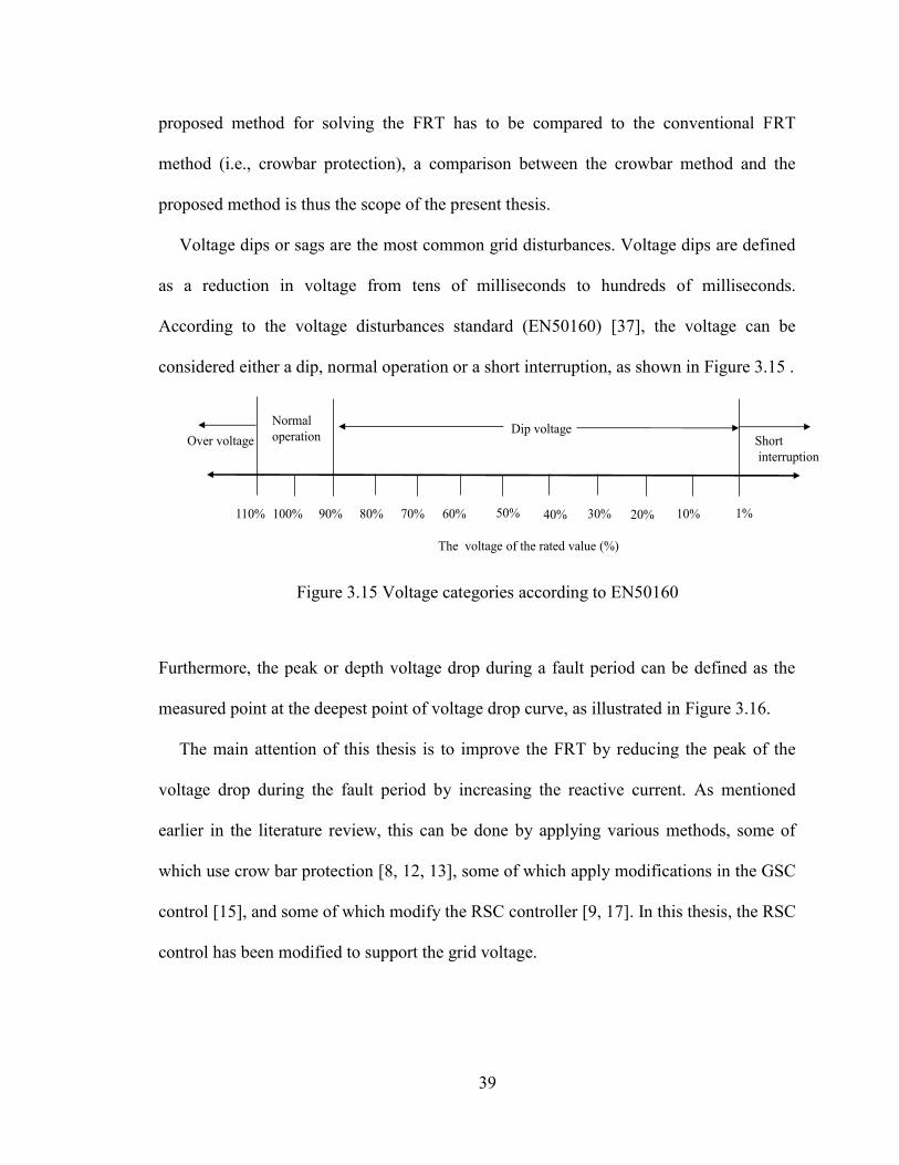
Voltage dips or sags are the most common grid disturbances. Voltage dips are defined

as a reduction in voltage from tens of milliseconds to hundreds of milliseconds.

According to the voltage disturbances standard (EN50160) [37], the voltage can be

considered either a dip, normal operation or a short interruption, as shown in Figure 3.15 .

Figure 3.15 Voltage categories according to EN50160

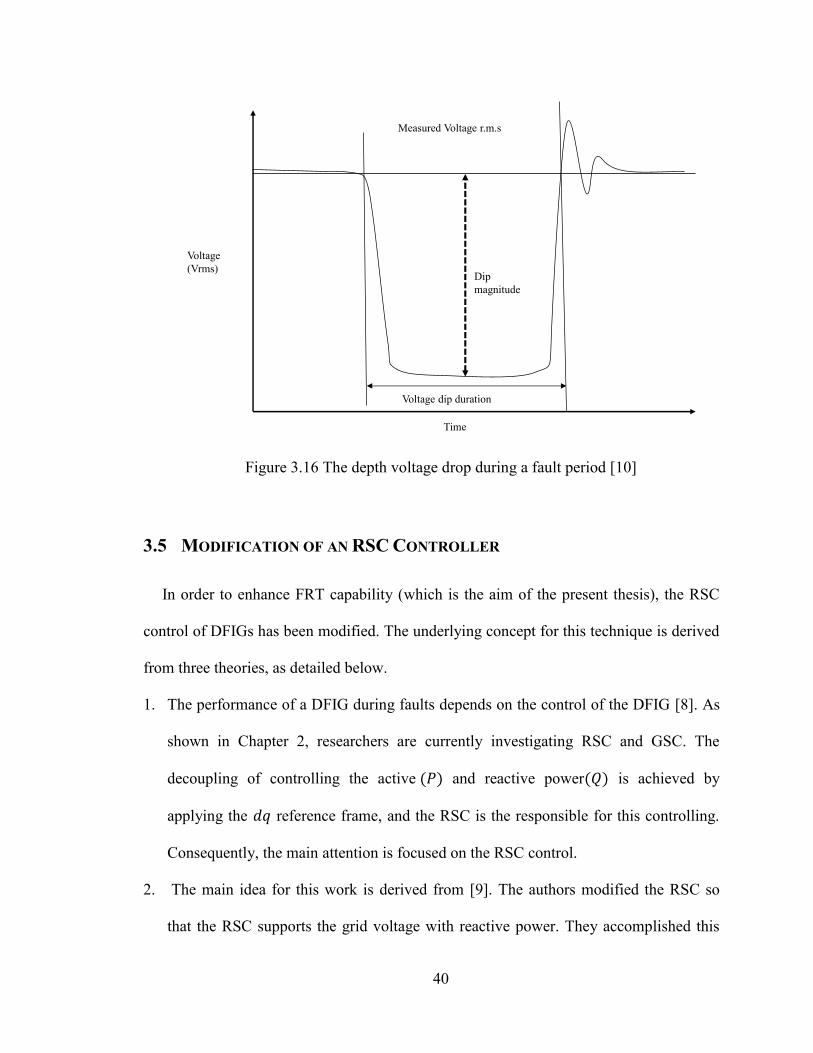
Furthermore, the peak or depth voltage drop during a fault period can be defined as the

measured point at the deepest point of voltage drop curve, as illustrated in Figure 3.16.

The main attention of this thesis is to improve the FRT by reducing the peak of the

voltage drop during the fault period by increasing the reactive current. As mentioned

earlier in the literature review, this can be done by applying various methods, some of

which use crow bar protection [8, 12, 13], some of which apply modifications in the GSC

control [15], and some of which modify the RSC controller [9, 17]. In this thesis, the RSC

control has been modified to support the grid voltage.

1%60%70%80%90%100% 50% 40% 30% 20% 10%110%

Dip voltageNormal

operation Short

interruption

Over voltage

The voltage of the rated value (%)

40

Figure 3.16 The depth voltage drop during a fault period [10]

3.5 MODIFICATION OF AN RSC CONTROLLER

In order to enhance FRT capability (which is the aim of the present thesis), the RSC

control of DFIGs has been modified. The underlying concept for this technique is derived

from three theories, as detailed below.

1. The performance of a DFIG during faults depends on the control of the DFIG [8]. As

shown in Chapter 2, researchers are currently investigating RSC and GSC. The

decoupling of controlling the active and reactive power is achieved by

applying the reference frame, and the RSC is the responsible for this controlling.

Consequently, the main attention is focused on the RSC control.

2. The main idea for this work is derived from [9]. The authors modified the RSC so

that the RSC supports the grid voltage with reactive power. They accomplished this

Voltage dip duration

Measured Voltage r.m.s

Voltage

(Vrms)Dip

magnitude

Time

41

by modeling the RSC control as a combination of three different controllers: an

electromagnetic torque controller, a current controller, and a voltage or reactive power

controller, as shown in Figure 3.17.

Figure 3.17 Three controllers are represented in the RSC controller [9]

The methodology of the electromagnetic torque controller, as Figure 3.18 shows, is to

track the mechanical power ( ) of the turbine with respect to the turbine speed ( .

This can be done by using the drive train, as explained in section 3.3.2. This speed is then

compared to the speed of the generator’s rotor ( ) through the PI controller, after

which the reference torque is determined, which is considered one of the inputs

of the current controller to determine the reference rotor current in the frame d ( ).

As mentioned earlier, during grid fault, a high speed of the generator’s rotor occurs.

Consequently, based on generator speed, the will be changed to support the grid

voltage.

RSCTorque

controller

RSC control

Current

controllerVoltage

controller

42

Figure 3.18 The electromagnetic torque and current controller

3. The drop voltage during the grid faults is a function of a fault current [10]

According to the three aspects listed above, instead of using an electromagnetic torque

controller to determine the reference rotor current ( based on the generator’s rotor

speed ( ), this thesis proposes that a new external circuit controller be applied to set

the reference of the current controller, as shown in Figure 3.19 .

Figure 3.19 The new proposed RSC controller

PI PI+

_

Electromagnetic torque controller Current controller

Drive train

_

+

RSC

RSC control

Current

controllerVoltage

controller

External circuit

controller

43

3.5.1 The New Proposed External Circuit

The main aim of this circuit is to determine the reference voltage of DFIG

which will be fed into the current controller to determine the during steady state as

well as during grid fault, as follows:

During normal operation, the is calculated by measuring the voltage at the

DFIG terminal ( ) and comparing it with the voltage at the point of common

coupling ( ) through a PI controller.

During grid fault, unlike in [9], the was adjusted to improve the FRT

capability of DFIG by relatively to the speed of the speed of the generator’s

rotor. In this thesis, and according to the third theory, the was adjusted by the

comparatively to the fault current , following the DFIG. Therefore, a

change in the reference voltage based on the will be proposed and

applied. Thus, the can be expressed by the fault current and a factor .

This factor is defined here as an impedance-type factor related to the change in the

reference voltage to the fault current. The is described by the following

equation (Ohm’s Law):

( 3-19)

where:

: the impedance-type factor

: the fault current

44

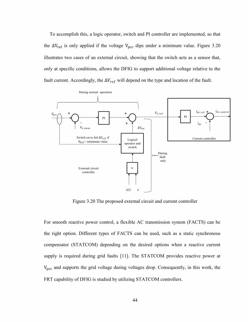
To accomplish this, a logic operator, switch and PI controller are implemented, so that

the is only applied if the voltage dips under a minimum value. Figure 3.20

illustrates two cases of an external circuit, showing that the switch acts as a sensor that,

only at specific conditions, allows the DFIG to support additional voltage relative to the

fault current. Accordingly, the will depend on the type and location of the fault.

Figure 3.20 The proposed external circuit and current controller

For smooth reactive power control, a flexible AC transmission system (FACTS) can be

the right option. Different types of FACTS can be used, such as a static synchronous

compensator (STATCOM) depending on the desired options when a reactive current

supply is required during grid faults [11]. The STATCOM provides reactive power at

and supports the grid voltage during voltages drop. Consequently, in this work, the

FRT capability of DFIG is studied by utilizing STATCOM controllers.

PI

Logical

operator and

switch

During normal operation

During

fault

only

Switch on to fed if

< minimum value

++

+-

PI

+

-

Current controller

External circuit

controller

45

3.6 THE STATCOM CONTROLLER.

The models of STATCOM controllers used in this thesis come from the

MATLAB/SIMULINK library [38]. This controller consists of a current controller and a

voltage controller. Additionally, the STATCOM controller is modeled in the reference

frame, as shown in Figure 3.21.

Figure 3.21 The STATCOM controller

As can be observed from Figure 3.21, the STATCOM controller is similar to the RSC

controller, differing only in how it defines the reference of the STATCOM controller

( ), as will be discussed later. The STATCOM located in the

MATLAB/SIMULINK library has as a feature, generated either by the

STATCOM itself or by an external value. Consequently, we exploited this advantage and

applied the proposed external circuit in a way similar to the RSC control to the

STATCOM control. In other words, we took into consideration that the is

computed by measuring the STATCOM voltage ( ) and compared it with

Current

controllerVoltage

controller STATCOM

STATCOM CONTROL

46

the voltage at the point of common coupling ( ), after which we injected the error

through a PI controller, as shown in Figure 3.22.

Figure 3.22 The proposed external circuit applied to the STATCOM controller

Consequently, by incorporating the two external circuits in Figure 3.20 and Figure 3.22

into one circuit, the new proposed external circuit was able to determine the and

of the RSC controller and STATCOM controller, respectively, as illustrated

in Figure 3.23.

PI

Logical

operator

and switch

During normal operation

During fault

only

Switch on to fed if

< minimum value

+

_

+

+

47

Figure 3.23 The proposed external circuit applied to the RSC and STATCOM controllers

Finally, this combined circuit was applied to the DFIG through the RSC controller and

the STATCOM controller to achieve the flowchart, as shown in Figure 3.24. From this

figure, the and can be determined by the external circuit, which is

considered the first stage. The second stage is the current controller and voltage controller

for both the RSC and STATCOM controllers. Figure 3.24 illustrates the methodology to

achieve the aim of this thesis, which is improving the FRT capability of DFIG-based

wind turbines.

PI

PI

Logical

operator

and

switch

Switch on to fed

if <

minimum value

During fault only

+

_

+

_

+

+

++

48

Figure 3.24 Voltage support at the point of common coupling by the DFIG and

STATCOM

3.7 SUMMARY

In this chapter, a brief introduction to wind turbine-based DFIGs was introduced. An

overview of wind turbine modeling was also provided, including the modelling of

aerodynamic and the mechanical components. As well, this chapter covered examples

showing the characteristics of a specific wind turbine, detailed the basic concept of DFIG

and the purpose for using as a reference frame, and demonstrated the dynamic fifth

order model of DFIG. Additionally, a brief introduction surrounding the behaviour and

mode of DFIG during grid disturbances was discussed.

STATCOM

PCC

DFIG

Grid

RSC

External

circuit

RSC control

Current

controllerVoltage

controller

Current

controllerVoltage

controller

STATCOM control

49

The main objective of this chapter was to present the external circuit as the

methodology used in this thesis. Hence, the modification of the RCC controller was

proposed and demonstrated, with the aim of improving the FRT capability of DFIG

during faults. All issues related to enhancing the FRT capability of a DFIG coupled to a

wind turbine during faults in next chapter are solved using the novel technique presented

in this chapter.

50

CHAPTER 4 RESULTS AND DISCUSSION

4.1 INTRODUCTION

In Chapter 3, the improvement of the FRT capability of DFIGs during faults by using

the external circuit method was introduced. In this chapter, the method will be

implemented in MATLAB/Simulink environment on a Lenovo laptop processor Intel core

2Duo with 2.00 GHz and 4.00 GB RAM, using a block in the MATLAB/Simulink library

[39], after which the results will be presented and discussed. The proposed method has

been applied to reduce the peak of the voltage drop during a fault period. In this chapter,

the results are presented to demonstrate the effectiveness of the method during faults, as

follows:

1. In case one, the effectiveness of the method is tested at point B during a fault,

as shown in Figure 4.1.

2. In case two, the effectiveness of the method is tested at PCC during a fault.

3. In case three, this method is compared to other methods to evaluate its

efficiency.

The results obtained are compared with results obtained without using the proposed

method, showing the method’s effectiveness in the depth point of the voltage drop.

4.2 DESCRIPTION OF THE SYSTEM

A one-line diagram of the system is shown in Figure 4.1. As we can see, a wind farm

of 9MW is connected to a 50Km distribution system. The distribution system is

represented by a 25KV.60Hz, translating power to a grid represented by 120 KV. A step-

down transformer 1 25KV/575V and transformer 2 120KV/ 25KV are applied. There are

51

five bus bars (B1, B2, B3, B4 and PCC) with voltages 575 V, 25KV, 25KV,120KV and

120 KV, respectively. As well, load and plant are connected to B1 and B3, respectively.

Figure 4.1 The system’s one-line diagram

A wind turbine using the DFIG consisting of a stator is connected directly to the grid. In

contrast, the rotor is connected to the grid via an AC/DC/AC IGBT-based pulse width

modulation (PWM) converter, as shown in Figure 4.2.

Figure 4.2 Wind turbines with doubly-fed induction generator [40]

DFIG

B1575 V

B225K V

B325K V

B4120K V120K V

S

T

A

T

C

O

M

10KM

40KM

AB

Grid

Equivalent

reactance

Transformer 2

120KV/25KVTransformer 1

25KV/575VGrid

120KV Wind farms

9MWPlant Load

52

The DFIG and wind turbine parameters are given in Appendix B. It should be

mentioned that these data are similar to the small power transmission system model

developed by mathworks in the Simpowersyst MATLAB/Simulink library [39]. In this

thesis, there is a slight modification of the RSC controller, as mentioned in Chapter 3.

Before studying the effect of the proposed method, more details about the other two

components of the RSC controller are given below.

From Figure 4.3, it can be concluded that the objective of the external circuit is to

generate the . This reference is injected to the current control through a PI

controller (V-regulator) to define the reference rotor current in frame (d) ). The

reference rotor current in frame (q) can be determined by controlling the active

power. By comparing these reference currents with the actual rotor currents ( , the

references of the voltage or reactive power control are achieved .

Furthermore, by injecting these values into the voltage controller through a PI controller

(I-regulator), the reference rotor voltages are determined ( , and by comparing

these reference voltages with the actual rotor voltages ( , the outputs of the RSC

controller are achieved .

53

Figure 4.3 The three components of the RSC controller

Immediately, transforming the from dq reference frame to abc frame and

then feeding them to a 3-phase PWM and subsequently to IGBTs with universal bridge. V

and I presented in the Figure 4.3 are represented the voltage and current at B1

respectively. The data of the external, current and voltage controllers are given in

Appendix B.

The wind turbine-based DFIG model and the external circuit in MATLAB/Simulink

are shown in Figure 4.4 and Figure 4.5, respectively. It should be noted that there is no

modification regarding the GSC controller, which already existed in [40]. As mentioned

in section 3.3.5, the duty of GSC is to keep the voltage of the DC-link constant.

Current controllerVoltage controller

RSC

PIdq

abc

External

circuit

Figure

3.23

PWM

+

+

+

-

-

PI

Current

measurement

Tracking

characteristic

PIPower looses

Power

measurement

+

-

-

Rotor

V-regulator

P-regulator

I-regulator

+

+

+

External circuit

controller

54

Figure 4.4 The MATLAB/Simulink model with the external circuit

Figure 4.5 The external circuit

55

4.3 CASE STUDIES

In this section, the dynamic interaction and performance of DFIG-based wind turbines

with power transmission systems during faults are illustrated and discussed. Three cases

will be simulated and studied. The objective of the first case is to test the proposed

method to improve the FRT capability of DFIGs at point B by considering a short-circuit

grid fault at the end of a 40Km transmission line at point A (close to PCC) and study the

voltage support during a fault. In the second case, the effect of the method at the PCC

during a fault will be studied and the results obtained when using the proposed external

circuit will be compared with those obtained when the proposed method is deactivated. In

the third case, the present method will be compared with other methods mentioned in the

literature review. To study faults, the DFIG and STATCOM models are set at a phasor

simulation type to allow transient stability studies with a long simulation time [39].

A short-circuit grid fault with fault resistance and ground resistance

occurs at point A at t=5 seconds, with a clearance time of 150(ms).

The wind speed is kept constant at 12(m/s). The proposed external circuit in Figure 3.23

is connected to the RSC of the DFIG and to the control circuit of STATCOM. It feeds the

whenever dips under a minimum value to support the system voltage.

According to Figure 3.15, this minimum value can be equal to 0.9(pu). Through trial and

error experiments, the impedance-type factor is rated at 0.2(pu), to give an optimum

value of . As a result, there is better voltage support to the grid, with being the

fault current flowing toward the DFIG, measured at B1. It shoud be mentioned that, the

results are within practical guidelines for circuit breaker allowable time limits.

56

4.3.1 Case study 1: Voltage Support at Point B During Grid Faults

As is generally known, voltage dips can be divided into two classifications: balanced

fault and unbalanced fault. Therefore, one-phase, two-phase, and three-phase grid faults

are applied at point A. Simulated results of these faults are presented in Figure 4.6, Figure

4.8 and Figure 4.10. In all fault test cases, comparisons of obtained results without using

the external circuit and with the proposed circuit results show that the proposed circuit

method achieves significantly better results regarding voltage support during grid fault. It

should be noted here that an external circuit case is simulated by connecting the external

circuit, and the obtained results show the effectiveness of the and STATCOM.

The response to , where the voltage at point B dips under 0.9(pu), is illustrated in

Figure 4.7, Figure 4.9 and Figure 4.11. From all of these figures, a variation of

between the different types of faults can be discerned. This is because the fault, , and

consequently the at the three-phase grid fault, are considered high. Hence, the

external proposed method has been successfully used to support voltage during grid fault

and improve the FRT, especially when three-phase faults occur, as Table 4.1 Comparison

between the voltage support of different types of faultsTable 4.1, Figure 4.12 and Figure

4.13 show. From this, it can be concluded that voltage support by the proposed external

circuit is done relative to the and subsequently to , as explained in the

methodology of this thesis.

57

Table 4.1 Comparison between the voltage support of different types of faults

Voltage at point (B)

The average of voltages obtained are within

prescribed standard limits (pu) Voltage support

(%) Without external circuit With external circuit

One-phase fault 0.7481 0.7533 0.52

Tow-phase fault 0.7438 0.7492 0.545

Three –phase fault 0.7428 0.7486 0.58

Figure 4.6 Positive sequence voltages at point B during a one-phase grid fault

4 4.5 5 5.5 6

0.75

0.8

0.85

0.9

0.95

1

Time(sec)

Vo

ltag

e a

t p

oin

t B

(p

u)

One-phase fault at the point A

With external circuit

Without external circuit

58

Figure 4.7 The response of ΔVref during one-phase grid fault

Figure 4.8 Positive sequence voltage at point B during a two-phase grid fault

4 4.5 5 5.5 60

0.02

0.04

0.06

0.08

0.1

0.12

0.14

0.16

Time(sec)

Dlt

a V

olt

ag

e (

pu

)

One-phase fault at the point A

During

fault

4 4.5 5 5.5 6

0.75

0.8

0.85

0.9

0.95

1

Time(sec)

Vo

ltag

e a

t p

oin

t B

(pu

)

Two-phase at the point A

With external circuit

Without external circuit

59

Figure 4.9 The response of ΔVref during two-phase grid fault

Figure 4.10 Positive sequence voltage at point B during a three-phase grid fault

4 4.5 5 5.5 60

0.02

0.04

0.06

0.08

0.1

0.12

0.14

0.16

0.18

Time(sec)

Dlt

a V

olt

ag

e (

pu

)

Two-phase fault at the point A

During

fault

4 4.5 5 5.5 6

0.75

0.8

0.85

0.9

0.95

1

Time(sec)

Vo

ltag

e a

t p

oin

t B

(p

u)

Three-phase fault at the point A

With external circuit

Without external circuit

60

Figure 4.11 The response of ΔVref during a one-phase grid fault

Figure 4.12 Comparison of the voltage drop between the three types of faults

4 4.5 5 5.5 60

0.02

0.04

0.06

0.08

0.1

0.12

0.14

0.16

0.18

0.2

Time(sec)

Dlt

a V

olt

ag

e (

pu

)

Three-phase fault at the point A

During

fault

0.736

0.738

0.74

0.742

0.744

0.746

0.748

0.75

0.752

0.754

0.756

One phase Two phase Three phase

Volt

age

dro

p (p

u)

Difrrent types of fault

with extenal circuit

without extenal circuit

61

Figure 4.13 Comparison of the voltage support between three different types of faults

when using the extenal circuit

4.3.2 Case study 2: Voltage Support at PCC During Grid Faults

In the present case, the external circuit is applied to enhance the FRT capability of

DFIG and support voltage at PCC during grid faults. Figure 4.14, Figure 4.15 and Figure

4.16 show a comparison between voltage recovery with and without using the proposed

method.

0.49

0.5

0.51

0.52

0.53

0.54

0.55

0.56

0.57

0.58

0.59

one phase two phase three phase

Volt

age

support

(%

)

Difreent types of fault

62

Figure 4.14 PCC voltage using the external circuit during a one-phase grid fault

Figure 4.15 PCC voltage using the external circuit during a two-phase grid fault

4 4.5 5 5.5 6

0.9

0.92

0.94

0.96

0.98

1

1.02

Time(sec)

Vo

ltag

e a

t P

CC

(p

u)

One-phase fault at the point A

With external circuit

Without external circuit

4 4.5 5 5.5 6

0.75

0.8

0.85

0.9

0.95

1

1.05

Time(sec)

Vo

ltag

e a

t P

CC

(p

u)

Two-phase fault at the point A

With external circuit

Without external circuit

63

Figure 4.16 PCC voltage using the external circuit voltage support during a three-phase

grid fault

Table 4.2 Comparison of voltage support during a fault with and without using the

external circuit

Voltage at PCC

The average of voltage obtained are within

prescribed standard limits (pu) Voltage support

(%) Without external circuit With external circuit

One-phase fault 0.8983 0.9015 0.3176

Two-phase fault 0.7539 0.7579 0.405

Three-phase fault 0.59 0.5944 0.4417

The following conclusions can be drawn from the results presented in Table 4.2. The

voltage support at the PCC is comparatively small; nevertheless, the results of the voltage

drop clearly show that the proposed external circuit has achieved significantly good

results in the FRT, especially when compared to results obtained without the external

4 4.5 5 5.5 6

0.6

0.65

0.7

0.75

0.8

0.85

0.9

0.95

1

Time(sec)

Vo

ltag

e a

t P

CC

(p

u)

Three-phase fault at the point A

With external circuit

Wthout external circuit

64

circuit. Moreover, the voltage support results show that the three-phase fault case has the

best voltage support compared to one- and two-phase faults due to the change of

according to . In the next subsection, the reactive power generated by the DFIG in a

different mode will be simulated and discussed.

4.3.2.1 The Reactive Power Generated by DFIG During FRT

In the following, the response of the DFIG with the external circuit during FRT under

three-phase grid faults is simulated and two different modes of DFIG (under-excited and

over-excited) are considered.

Before and after a fault occurred, as shown in Figure 4.17, the DFIG in under-excited

mode, which means, the DFIG will attempt to absorb the reactive power (see Figure 3.13)

around 1.3MVAr limits. During a fault, a fault current flows from the grid into the DFIG.

In this state, the DFIG will generate and supply reactive power by the RSC, this can be

done by using the temporary overload capability of DFIG [11] in order to support grid

voltage recovery. Likewise, when the DFIG is in over-excited mode (as illustrated in

Figure 4.18) before and after the fault occurred, the DFIG (according to Figure 3.13)

supply around 1.8MVAr reactive power to raise the grid voltage. In fault instance, same

way of the above case ,the DFIG will generate and supply reactive power To sum up, for

both modes of DFIG during a grid fault, the DFIG would fulfill the grid requirement and

supply the system via reactive power.

65

Figure 4.17 Reactive power generated by DFIG at under-excited mode and during FRT

Figure 4.18 Reactive power generated by DFIG over-excited mode and during FRT

0 1 2 3 4 5 6 7 8 9 10-4

-2

0

2

4

6

8

Time(sec)

Reacti

ve p

ow

er

gen

era

ted

by

DF

IG

Three phase grid fault

Under-excited mode

0 1 2 3 4 5 6 7 8 9

-2

0

2

4

6

8

Time(sec)

Reacti

ve p

ow

er

gen

era

ted

by

DF

IG

Three phase grid fault

Over-excited mode

66

Figure 4.19 shows the reactive power supplied by both modes during FRT. As can be

observed, the DFIG in under-excited mode supplies more reactive power than in-over

excited mode, proving one of the characteristics of the DFIG stated in Chapter 3.

Figure 4.19 Average reactive power supplied during FRT for different modes of DFIG

As a final point in this subsection, comparisons will be simulated to check the

effectiveness of the external circuit on reactive power supplied by the DFIG in unity

mode. Two different scenarios are analysed – the first scenario is without the external

circuit and second one is with the external circuit. Both scenarios are illustrated in Figure

4.20. As can be seen, the reactive power supplied in the second scenario is substantially

higher than power supplied in the first. This result explains why the voltage dips in the

second scenario are frequently smaller than in the first scenario.

4.804

5.043

4.65

4.7

4.75

4.8

4.85

4.9

4.95

5

5.05

5.1

over excitedmode

underer excitedmode

67

Figure 4.20 Reactive power generated by the DFIG at unity mode and during FRT

4.3.3 Case study 3: Evaluation of the Method

In order to test the effectiveness of the proposed external circuit during a grid fault, the

proposed method will be compared to the crowbar protection method, after which the

impact of will be discussed. Subsequently, a comparison between current and novel

methods, as listed in Chapter 2, is provided.

4.3.3.1 The Impact of Crowbar Activation During FRT

The crowbar impact was reported in detail in Chapter 2 and its disadvantages were

summarized in Chapter 3. In this section, to demonstrate the undesirable effect of crowbar

protection on voltage recovery during a fault, voltage support is simulated by activating

crowbar during a one-phase grid fault at point A. Here, the activation of crowbar can be

3 3.5 4 4.5 5 5.5 6 6.5 7 7.5

0

1

2

3

4

5

6

7

Time(sec)

Reacti

ve p

ow

er

gen

era

ted

by

DF

IG

Three phase grid fault

With external circuit

Without external circuit

At unity mode

68

occur in two situations: (1) when the rotor current increases and exceeds the maximum

limit; and (2) when the DC-link voltage increases and overshoots the maximum limit [9].

In this thesis, the second situation is simulated. Basically, in a fault instant, the DFIG

draws fault currents from the grid into the DC-link located in the converter. These

currents reverse the diodes which are connected with IGBTs, causing a high voltage of

the DC-link. As a result, the crowbar protection circuit will be switched on and activated

[11].

To do this, in the protection system of the MATLAB/Simulink model in Figure 4.4,

the DC-link voltage is set to maximum value so that, during grid fault, the DC-link

voltage will exceed this maximum value. A simulation of the system is carried out in

Figure 4.21, where it can be seen that the fault happens at 5(sec) with crowbar protection.

Additionally, the figure shows the voltage at PCC before and after the fault, with a

comparison between the proposed external circuit and the crowbar method.

69

Figure 4.21 Voltage at PCC using different methods of FRT for improvement

Table 4.3 Comparison of PCC voltages between different cases of FRT to FRT with

crowbar

Voltage at PCC (pu)

Voltages obtained are within prescribed standard limits

With external circuit With crowbar protection

One-phase fault 0.9057 0.8966

The following conclusions can be drawn from the results presented in Table 4.3. The

voltage dip at PCC during a fault is around 0.8966( ) when the crowbar circuit is

activated. This can be considered the worst case scenario because the controllability of

DFIG is lost and the DFIG would behave as a squirrel cage induction generator; however,

with the proposed external circuit, the dip is around 0.9057( ). Consequently, it can be

concluded that the best FRT can be achieved without crowbar protection. Indeed, [11]

4 4.5 5 5.5 6

0.9

0.92

0.94

0.96

0.98

1

1.02

Time (sec)

Vo

ltag

e a

t P

CC

(pu

)

One-phase fault at the point A

with external circuit

with crowbar

70

reported that the majority of modern wind turbines coupled to DFIG attempt to ride

through the fault without activating the crowbar.

4.3.3.2 The Impact of the Delta Reference Voltage

In this subsection, the evaluation of the weight of is presented. The simulations

were first done without connecting the of the external circuit to the STATCOM and

RSC controllers. in other words, during FRT, the was deactivated. Next, in

comparing the results obtained from the above to the results obtained when using the

entire circuit (including the ) it is clear that, during a grid fault, the lowest voltage

dip of 0.78( ) at 5.1(sec) occurs when the is deactivated. On the other hand, the

voltage dip improves dramatically – to about 0.79 ( ) – when the is activated .as

Figure 4.22 shows

Figure 4.22 The effect of deactivating the ΔVref

4 4.5 5 5.5 6

0.75

0.8

0.85

0.9

0.95

1

1.05

Time(sec)

Vo

ltag

e a

t P

CC

Two -phase fault at the point A

FRT without Delta reference voltage

FRT with Delta reference voltage

71

4.3.3.3 Comparison Between the External Circuit Method and Various FRT

Methods

In this subsection, the FRT obtained by the proposed method is compared with some

other methods listed in the literature review [9]. The researchers also modified the RSC

controller and used the STATCOM to study the FRT capability of DFIG at (B1).

Therefore, the voltage at B1, which is called the DFIG terminal, will be simulated during

a three-phase grid fault and two different cases are implemented. The first case is without

the external circuit and the second case is with it, as shown in Figure 4.23.

Figure 4.23 Voltage at a DFIG terminal during a three-phase grid fault

Before and after the fault, the voltage at the DFIG terminal in the second case is the

higher compared to the first case. During the fault, the first case has the lowest voltage

dip of 0.68 ( ) at 5.04 (sec). In contrast, the voltage dip improved significantly to 0.7 at

5.04(sec) in the second case.

4 4.5 5 5.5 6

0.7

0.75

0.8

0.85

0.9

0.95

1

1.05

1.1

Time(sec)

Vo

ltag

e a

t D

FIG

term

inal

Three-phase grid fault

Without external circuit

With external circuit

72

In [9], two additional cases were analyzed. The first case featured no voltage support

and the second case featured modified RSC control and STATCOM. During the fault, the

first case showed a voltage dip of 0.53 ( ) at 5.03, while in the second there was no

indication of the value of the voltage drop. To find the value, Graph Click software was

utilized and revealed voltage drop to be around 0.55 ( ). A comparison of the two

methods is illustrated in Table 4.4.

Table 4.4 Comparison of the voltage support obtained by the proposed method and the

method in [9]

Method

Modification

of RSC

controller

Methodology

of voltage

support

Average voltages

obtained are

within prescribed

standard limits

( )

Voltage

support

during fault

(%)

Reactive

power

source

1. [9]

Combined from

electromagnetic

torque, current,

and voltage

controllers

Relative to

generator

speed

without 0.53( )

2% STATCOM

with 0.55( )

2. External

circuit

Combined from

external circuit,

current, and

voltage

controllers

Relative to

generator

fault current

without 0.68( )

2% STATCOM

with 0.70( )

The following conclusions can be drawn from the results presented in Table 4.4:

1. The comparison shows that the RSC controller for both methods has been modified

and combines three different controllers. The difference, in this thesis, is that an

73

alternative external circuit is used to support grid voltage instead of the

electromagnetic torque controller.

2. This comparison clarifies that the methodology used in the first method to support the

grid voltage is relative to the generator speed. However, in this work, the

methodology to support the grid depends on the generator fault current.

3. This comparison indicates that the two methods have the same improvement in FRT

capability of the wind turbine-based DFIG with 2% during a grid fault.

Consequently, it can be observed that improvements to the FRT capability of the DFIG

including voltage support achieved by [9] can also be obtained by the proposed external

circuit.

This technique has advantages since using current as a feedback, so the variable is less

complex that using the electromagnetic torque method.

Furthermore, the proposed method supports the voltage by 0.02 (pu), meaning 15% of

the rated voltage 1(pu). Therefore, the proposed method successfully satisfied grid code

requirements which requests an FRT capability of up to 15 % of retaining voltage [14].

In this thesis, STATCOM is the only reactive power source used to support grid

voltage. The unique point is to take advantage of the DFIG during a fault when switching

to over-excited mode to support the reactive power. At this particular moment, the

is applied to adjust the reference voltages of the STATCOM and RSC controllers. On the

other hand, the high cost of using STATCOM may be considered a disadvantage.

4.4 SUMMARY

In this chapter, improvements to the FRT capability of the DFIG during grid fault were

tested and confirmed on a wind turbine, and the objective (namely, the reduction of the

74

voltage drop peak during grid fault) was obtained with the proposed external circuit.

Furthermore, the FRT issue was initially improved at a specific point on the transmission

lines and then improved at PCC. The impact of the crowbar was also discussed. A

comparison with other methods shows that the proposed method has achieved the same

results in voltage support at DFIG terminals.

75

CHAPTER 5 CONCLUSION AND FUTURE WORK

5.1 CONCLUSION

Overcoming limitations and issues related to the FRT capability of the DFIG is

currently a prime topic of research, and many techniques have been proposed in this area.

In this present work, the FRT issue was enhanced by using the proposed external circuit.

Earlier in the thesis, the aerodynamic model of a wind turbine was discussed and

analyzed because it is required for simulating FRT capability during grid faults, as are

the mechanical and electrical components presented in this thesis. Currently, due to

increased implementation of wind turbines, most system operators demand that a wind

turbine supply reactive power during a fault in order to support the voltage recovery. For

a fixed wind turbine, there are numerous options for fulfilling the requirements of reactive

power, the best one of which uses FACTS controllers. However, for a DFIG coupled to a

wind turbine, this compensation can be achieved with the assistance of a back-to-back

converter as well FACTS controllers. Consequently, the RSC controller is modified in

this study to support the grid voltage and improve FRT capability during a fault.

An external circuit was applied to a DFIG-based wind turbine connected to a power

system. This was then validated by improving the FRT at the PCC and DFIG terminals

during a grid fault, clearly demonstrating the efficacy of the proposed method, as the

external circuit successfully improved the FRT. The impact of the crowbar protection

method on FRT was also discussed and compared with the external circuit method.

The capability of the external circuit to improve voltage support during a fault has

been affirmed and compared to similar methods. According to the results obtained, it can

76

be concluded that a proper setting of the external circuit, including the controllers, may be

integrated to the RSC controller of the DFIG to achieve results that are equivalent to

those created by an electromagnetic torque controller applied to an RSC controller.

The literature review in this thesis demonstrated the current and past methods used to

address and resolve issues related to FRT capability of DFIG wind turbines. The focus of

this thesis was thus how to improve the FRT in light of the issues discussed in the review.

5.2 FUTURE WORK

The area of study encompassed by this thesis and the solutions and methods explored

in this work can be further expanded to further research areas, as per the following

suggestions:

The issue of FRT capability of DFIGs during grid faults can be reconsidered using

alternative combination approaches, such as united power flow controllers (UPFC)

and other reactive power sources.

The management of reactive power from wind farm providers could be considered a

non-liner optimization problem. Hence, an optimization method such as modified

bacterial foraging algorithm (MBFA) could be used to solve this task.

The performance of the external circuit presented in this thesis can be compared with

other techniques.

77

REFERENCES

[1] B. Chitti Babu, and K.B.Mohanty. "Doubly-fed induction generator for variable speed

wind energy conversion systems-modeling & simulation." International Journal of

Computer and Electrical Engineering, vol. 2, no. 1, pp. 1793-8163, 2010.

[2] Siret, "The wind turbines and wind farms database." Internet:

http://www.thewindpower.net/index.php, Sep.2012 [Oct.2012]

[3] Simoes, M. Godoy, and Felix A. Farret. Renewable energy systems. 2004:CRC.

[4] S. Muller, M. Deicke and R. W. De Doncker. "Doubly fed induction generator

systems for wind turbines." Industry Applications Magazine, IEEE, vol. 8, no. 3, pp. 26-

33, 2002.

[5] J. B. Ekanayake, L. Holdsworth and N. Jenkins." Comparison of 5th order and 3rd

order machine models for doubly fed induction generator (DFIG) wind turbines." Electr.

Power Syst. Res, vol. 67, no. 3, pp. 207-215,2003.

[6] Staff of lab-volt, "Principles of doubly-fed induction generator," Lab-volt electric

power technology training program, Canada, Tech. Rep. 86376-F0. 2011.

[7] Jia, X., Tian L., Xing Z. X., Su X. B., "Dynamic Model and Simalation of Double

Feed Induction Generator Wind Turbine," IEEE International Conferences on

Automation and Logistics, pp.1667-1671, 2009.

[8] A. D. Hansen and G. Michalke. "Fault ride-through capability of DFIG wind

turbines." Renewable Energy, vol. 32, no. 9, pp. 1594-1610, 2007.

[9] K. Ahsanullah and J. Ravishankar, "Fault ride-through of doubly-fed induction

generators," in Proc. of Int. Conference on Power, Signals, Controls and Computation

(EPSCICON), 2012, pp. 1-6.

[10] G. Abad, J. Lop'ez, M. Rodriguez, L. Marroyo and G. Iwanski. Doubly Fed

Induction Machine Modeling and Control for Wind Energy Generation. Hoboken,New

Jersey: John wiley&sons, 2011.

[11] M. Wilch, V.S. Pappala, S.N. Singh, I. Erlich. "Reactive power generation by dfig

based wind farms with ac grid connection," Power Tech, 2007, IEEE, Lausanne (2007),

pp. 626–632.

[12] M.Seyedi. "Evaluation of the DFIG wind Turbine Built-in Model in

PSS/E,"M.A.thesis, Chalmers University of Technology, Sweden, 2009.

78

[13] S. Seman , J. Niiranen , S. Kanerva , A. Arkkio and J. Saitz. "Performance study of

a double fed wind-power induction generator under network disturbances." IEEE

Transactions. Energy Conversion, vol. 21, no. 4, pp. 883 -890, 2006.

[14] A. Dittrich and A. Stoev. "Comparison of fault ride-through for wind turbines with

DFIM generators," in proc. 11th Eur. Conf. Power Electron. Appl., pp. 1 -8, 2005.

[15] L. Zhang, X. Jin and L. Zhan. "Reactive power control of doubly fed induction

generator during grid voltage dips," in proc.APPEEC 2012 Power and Energy

Engineering Conference , 2012.

[16] S. Seman, J. Niiranen and A. Arkkio. "Ride-through analysis of doubly fed induction

wind-power generator under unsymmetrical network disturbance." Power Systems, IEEE

Transactions, vol. 21, no 4, pp. 1782-1789, 2006.

[17] Dawei Xiang, Li Ran, P. J. Tavner and S. Yang. "Control of a doubly fed induction

generator in a wind turbine during grid fault ride-through." Energy Conversion, IEEE

Transactions, vol. 21,no. 3, pp. 652-662, 2006.

[18] Jin Yang, J. E. Fletcher and J. O'Reilly. "A series-dynamic-resistor-based converter

protection scheme for doubly-fed induction generator during various fault conditions."

Energy Conversion, IEEE Transactions, vol. 25, no.2 , pp. 422-432,2010.

[19] B. Gong, D. Xu and B. Wu. "Cost effective method for DFIG fault ride-through

during symmetrical voltage dip,"in proc.IECON 2010,36th Annual Conference on IEEE

Industrial Electronics Society, pp. 3269-3274, 2010.

[20] C. Zhan and C. D. Barker. "Fault ride-through capability investigation of a doubly-

fed induction generator with an additional series-connected voltage source converter.

Presented at AC and DC Power Transmission,"in proc.ACDC 2006, 8th IEE International

Conference , pp.79 -84, 2006.

[21] J. Morneau, C. Abbey and G. Joos." Effect of low voltage ride through technologies

on wind farm,"in proc.Electrical Power Conference, 2007. EPC 2007. IEEE Canada,

pp.56 -61 ,2007 .

[22] N. Joshi and N. Mohan. "A novel scheme to connect wind turbines to the power grid.

Energy Conversion," IEEE Transactions, vol.24, no.2, pp. 504-510,2009.

[23] S. Santoso and H. T. Le. "Fundamental time–domain wind turbine models for wind

power studies," Renewable Energy, vol. 32,no. 14, pp. 2436-2452. 2007.

[24] Heier, Siegfried. Grid integration of wind energy conversion systems. Hoboken:

Wiley, 1998.

79

[25] Patel, Mukund R. Wind and solar power systems: design, analysis, and operation.

CRC, 2005.

[26] "Wind turbine implement model of variable pitch wind turbine." Internet:

Http://www. Mathworks. Com.

[27] J. G. Slootweg, H. Polinder and W. L. Kling. "Dynamic modelling of a wind turbine

with doubly fed induction generator," in proc. Power Engineering Society Summer

Meeting, 2001.

[28] H. H. Aly and M. E. El-Hawary. "An overview of offshore wind electric energy

resources," in proc. Electrical and Computer Engineering (CCECE), 2010 23rd Canadian

Conference ,2010.

[29] F. Mei and B. C. Pal. "Modelling and small-signal analysis of a grid connected

doubly-fed induction generator," in proc. Power Engineering Society General Meeting,

2005. IEEE, pp.358 -367 ,2005.

[30] F. Iov, A.D. Hansen, P. Sørensen and F. Blaabjerg, "Wind Turbine Blockset in

Matlab/Simulink. General Overview and Description of the Models", Aalborg University,

March 2004, ISBN 87-89179-46-3.

[31] J. B. Ekanayake, L. Holdsworth, X. G. Wu and N. Jenkins. "Dynamic modeling of

doubly fed induction generator wind turbines," Power Systems, IEEE Transactions,vol.

18,no. 2,pp. 803-809. 2003.

[32] J. B. Ekanayake, L. Holdsworth and N. Jenkins. "Comparison of 5th order and 3rd

order machine models for doubly fed induction generator (DFIG) wind turbines," Electr.

Power Syst. Res. vol. 67,no. 3, pp. 207-215. 2003.

[33] B. Dosijanoski. "Simulation of Doubly-Fed Induction Generator in a Wind Turbine,

" in proc. XI International PhD Workshop,OWD 2009, pp. 378-383,2009.

[34] H. Camille. "Doubly-fed Induction Generator Modeling and Control in DigSilent

Power Factory," M.A. thesis, KTH School of Electrical Engineering, 2010.

[35] M. Milosevic. "Decoupling Control of d and q Current Components in Three-Phase

Voltage Source Inverter," Technical Report, 2003.

[36] E.on Netz Grid Code,"High and extra high voltage." Internet:

http://www.pvupscale.org/IMG/pdf/D4_2_DE_annex_A3_EON_HV_grid__connection_r

equirements_ENENARHS2006de.pdf , 2006.

[37] H.Markiewicz and A.Klajn . " Voltage Disturbances Standard EN 50160 -Voltage

Characteristics in Public Distribution Systems," Technical Report, 2004.

80

[38]http://www.mathworks.com/help/physmod/powersys/ref/staticsynchronouscompensat

orphasortype.html

[39]http://www.mathworks.com/help/physmod/powersys/ug/wind-farm-using-doubly-

fed-induction-generators.html

[40]http://www.mathworks.com/help/physmod/powersys/ref/windturbinedoublyfedinduct

iongeneratorphasortype.html

81

APPENDIX A

The following MATLAB code was used to draw the performance coefficient ) as a

function of tip speed ratio ( ) with pitch angle ( as parameter in addition to extract the

(base) and ( base) when

B=0; for m=1:15 H(m)=1/(m+0.08*B)-0.035/(B*B*B+1); l(m)=1/H(m);

cp(m)=0.5176*(116/l(m)-0.4*B-5)*exp(-21/l(m))+0.0068*m; end m=[1:1:15]; plot(m,cp(m)); grid [cpmax,mmx]=max(cp(m)) xlabel('Tip speed ratio lmbdas') ylabel(' Performance coefficient cp') text(7,0.55,'0 deg')

B=2; for m=1:15 H(m)=1/(m+0.08*B)-0.035/(B*B*B+1); l(m)=1/H(m);

cp(m)=0.5176*(116/l(m)-0.4*B-5)*exp(-21/l(m))+0.0068*m; end m=[1:1:15]; hold on plot(m,cp(m)); text(10.2,0.49 ,'{2 deg}')

B=5; for m=1:15 H(m)=1/(m+0.08*B)-0.035/(B*B*B+1); l(m)=1/H(m);

cp(m)=0.5176*(116/l(m)-0.4*B-5)*exp(-21/l(m))+0.0068*m; end

82

m=[1:1:15]; hold on plot(m,cp(m)); text(13.2,0.3 ,'{5 deg}')

B=10; for m=1:15 H(m)=1/(m+0.08*B)-0.035/(B*B*B+1); l(m)=1/H(m);

cp(m)=0.5176*(116/l(m)-0.4*B-5)*exp(-21/l(m))+0.0068*m; end m=[1:1:15]; hold on plot(m,cp(m)); text(8,0.3 ,'{10 deg}')

B=15; for m=1:15 H(m)=1/(m+0.08*B)-0.035/(B*B*B+1); l(m)=1/H(m);

cp(m)=0.5176*(116/l(m)-0.4*B-5)*exp(-21/l(m))+0.0068*m; end m=[1:1:15]; hold on plot(m,cp(m)); text(8,0.17 ,'{15 deg}')

B=20; for m=1:15 H(m)=1/(m+0.08*B)-0.035/(B*B*B+1); l(m)=1/H(m);

cp(m)=0.5176*(116/l(m)-0.4*B-5)*exp(-21/l(m))+0.0068*m; end m=[1:1:15]; hold on plot(m,cp(m)); text(7,0.1 ,'{20 deg}')

83

APPENDIX B

Table (C1) A wind turbine and power transmission system Data are below

Wind Turbine Data

Base mechanical power

The wind speed 12m/s

Power Transmission System Data

Bus bare (B1) 575(V)

Bus bare (B2) 25(KV)

Bus bare (B3) 25(KV)

Bus bare (B4) 120(KV)

Bus bare of point of common coupling 120(KV)

Load 500(KW)

Plant 2(MVA)

Transformer 1 25KV/575V,

Transformer 2 120KV/25KV,

Line 1 10( Km)

Line 2 40(Km)

Grid 120(KV), 60(Hz)

Grid equivalent reactance Zero sequence parameters/positive

sequence parameters=3

Table (C2) A DFIG, parameters of RSC controller and parameters of GSC controller

Data.

DFIG Data

Base power

⁄ (VAR)

Base line to line voltage 575 ( V)

The stator resistance in per unit ( 0.00706

The stator inductance in per unit ( 0.171

84

The rotor resistance in per unit 0.005

The rotor inductance in per unit 0.156

The mutual inductance in per unit 2.9

Base Frequency 60

The number of the poles 3

Inertia constant 5.04

Fraction 0.01

Parameters of RSC controller Data

voltage regulator 1.5 300

Power regulator 1 100

Current regulator 0.3 8

Parameters of GSC controller Data

Dc –voltage regulator 0.002 0.05

Current regulator 1 100

Droop 0.02

Table (C3) An external circuit Data.

Generator side regulator 70 14

STATCOM side regulator 0.316 1e-004

Critical value 0.9

STATCOM 100

The impedance type factor 0.2