Fault Analysis of Heglig Basin Network

A thesis submitted

by

Ahmed Abdel Razig Mohamed

B.Sc (Electrical and Electronic Eng. ,

University of Kharkov).

In fulfillment of the requirements for the degree of Master of

Science in Electrical and Electronic Engineering.

Department of Electrical and Electronic Engineering,

Faculty of Engineering and Architecture,

University of Khartoum.

March 2006

Dedication

gÉ Åç Ytà{xÜ

gÉ Åç `Éà{xÜ

gÉ Åç ã|yx tÇw Åç fÉÇá

Acknowledgement

I would like to express my deep appreciation and

gratitude to my supervisors Professor. Alamin Hamoda &

Dr. Kamal Ramadan who helped me greatly and for their

effort and guidance.

Special thanks are also due to my colleagues ;Alsadig

Hassan ,Muaz Abd Allah and Mutawakil Dafalla, for

their valuable assistance and continuous encouragement.

Thanks are also due to my family, friends and to whomever

had helped or encouraged me during my study.

Thank to God for helping me to complete this study.

بسم اهللا الرحمن الرحيم

ملخص البحث

سنويا في شبكة هجليج بسبب الطيـو او غيرهـا عطال التي تحدث األ ان

نقطـاع نتـاج نتيجـة إل تؤدي فى مجملها إلنخفاض معدالت اإل لكوابلكأعطال ا

كم طائـل سنويا )النيل الكبرى ( الشركة مداد الكهربائي من الحقول وبالتالي تفقد اإل

عطـال أهمية دراسـة هـذه األ من العملة الصعبة بسبب هذه المشكلة لذا برزت

. ووضع الحلول المناسبة لها

في هـذا المجـال بعدة معالجات مع االستعانة ببيوت الخبرة قامت الشركة

نتائج ايجابية الخارجية منها و الداخلية كجامعة الخرطوم على سبيل المثال اعطت

. ولكنها لم تقضي نهائيا على المشكلة

ان كل المعالجات التي تمت سابقا كلها تمثلت في التصميم والتركيب أما في

هذا البحث تم وضع دراسة تعتبر مكملة للدراسات السابقة حيث يتم تحليل األعطال

بـصورة بواسطة برنامج كمبيوتر مما يساعد في تحليل النظام واختيار األجهـزة

سليمة وكذلك أجهزة الحماية مع توفير المعلومات الالزمة للخطط المستقبلية لتمديد

. اوتعديل في النظام مما يقود لنظام آمن ومستقر

ABSTRACT

The huge number of power trips which have been experienced in

Heglig Power System, by birds or other reasons; such as, cable

termination failures, has caused a large production deficit which costs

(GNPOC) a large amount of dollars annually.

GNPOC experts have proposed some practical solutions to put an

end; or at least to minimize this number of trips. Different auditors were

invited to engineering workshops from overseas and in-house one of them

was Khartoum University. The result of this, has minimized the number

of trips, to some extent, but has not eliminated them. The majority of

proposals that were presented by the auditors dealt with problems which

are linked to design and construction.

This thesis has been conducted, using the established methods and

procedures, to show the main faults and causes; and also to analyse the

Heglig Grid, with the aid of the computer program .The information

gained from fault studies can be used for any network analysis and design

and also for nominal capacities of the existing equipment. Also; they can

be used for planning systems which lead to the stability of the system.

Moreove; this study will be more useful and effective ,if it is used;

together with other previous studies.

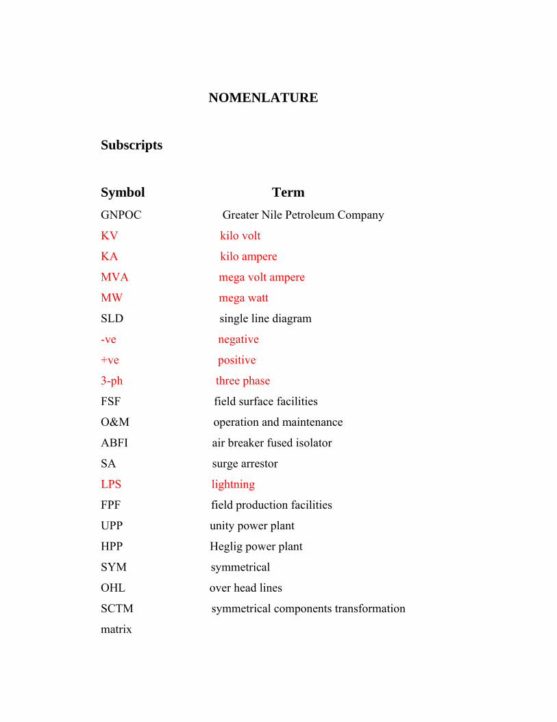
NOMENLATURE

Subscripts

Symbol Term GNPOC Greater Nile Petroleum Company

KV kilo volt

KA kilo ampere

MVA mega volt ampere

MW mega watt

SLD single line diagram

-ve negative

+ve positive

3-ph three phase

FSF field surface facilities

O&M operation and maintenance

ABFI air breaker fused isolator

SA surge arrestor

LPS lightning

FPF field production facilities

UPP unity power plant

HPP Heglig power plant

SYM symmetrical

OHL over head lines

SCTM symmetrical components transformation

matrix

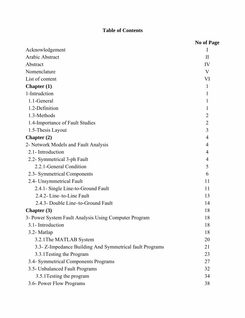
Table of Contents

No of PageAcknowledgement I Arabic Abstract II Abstract IV Nomenclature V List of content VI Chapter (1) 1 1-Intrudction 1 1.1-General 1 1.2-Definition 1 1.3-Methods 2 1.4-Importance of Fault Studies 2 1.5-Thesis Layout 3 Chapter (2) 4 2- Network Models and Fault Analysis 4 2.1- Introduction 4 2.2- Symmetrical 3-ph Fault 4 2.2.1-General Condition 5 2.3- Symmetrical Components 6 2.4- Unsymmetrical Fault 11 2.4.1- Single Line-to-Ground Fault 11

2.4.2- Line–to-Line Fault 13 2.4.3- Double Line–to-Ground Fault 14

Chapter (3) 18 3- Power System Fault Analysis Using Computer Program 18 3.1- Introduction 18 3.2- Matlap 18 3.2.1The MATLAB System 20 3.3- Z-Impedance Building And Symmetrical fault Programs 21 3.3.1Testing the Program 23 3.4- Symmetrical Components Programs 27 3.5- Unbalanced Fault Programs 32

3.5.1Testing the program 34 3.6- Power Flow Programs 38

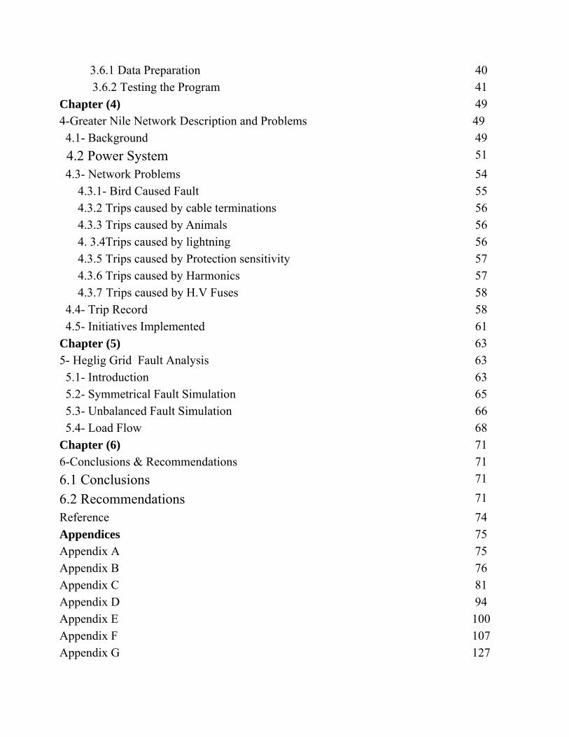
3.6.1 Data Preparation 40 3.6.2 Testing the Program 41

Chapter (4) 49 4-Greater Nile Network Description and Problems 49 4.1- Background 49 4.2 Power System 51 4.3- Network Problems 54 4.3.1- Bird Caused Fault 55 4.3.2 Trips caused by cable terminations 56 4.3.3 Trips caused by Animals 56 4. 3.4Trips caused by lightning 56 4.3.5 Trips caused by Protection sensitivity 57 4.3.6 Trips caused by Harmonics 57 4.3.7 Trips caused by H.V Fuses 58 4.4- Trip Record 58 4.5- Initiatives Implemented 61 Chapter (5) 63 5- Heglig Grid Fault Analysis 63 5.1- Introduction 63 5.2- Symmetrical Fault Simulation 65 5.3- Unbalanced Fault Simulation 66 5.4- Load Flow 68 Chapter (6) 71 6-Conclusions & Recommendations 71 6.1 Conclusions 71

6.2 Recommendations 71 Reference 74 Appendices 75 Appendix A 75 Appendix B 76 Appendix C 81 Appendix D 94 Appendix E 100 Appendix F 107 Appendix G 127

Introduction

1.1 General Analysis of fault level, pre-fault condition, and post-fault condition

are required for the selection of interruption devices, protective relays,

switchgears and measuring equipments and their coordination. Systems

must be able to withstand certain limits of faults which also affect

reliability indices. Many classical studies have been carried out on this

topic. This project seeks to conduct a comprehensive fault level

calculation and the effect of fault current by the aid of computer program

(MATLAP), for the HEGLIG GRID.

1.2 Definitions

A fault in electrical equipment is defined as a defect in its electrical

circuit due to which the current is diverted from the intended path. Faults

are generally caused by breaking of conductors or failure of insulation.

Other causes of faults include mechanical failure, accidents, excessive

internal and external stresses, etc. The fault impedance being low, the

fault currents are relatively high. During the faults, the voltages of the

three phases become unbalanced. The fault currents being excessive, they

can damage the faulty equipment and the supply installation. During the

faults, the power flow is diverted towards the fault and the supply to the

neighboring zone is affected .The faults can be minimized by improving

the system, design and quality of the equipment and maintenance.

However the faults cannot be eliminated completely

The fault currents can damage the equipment; and the supply

installation, if allowed to flow for long duration. In order to avoid such

damage, every part of the power system is provided with a protective

relaying system and associated switching device. The protective relays

are automatic devices which can sense the fault and send instructions to

the associated circuit-breaker to open the circuit breaker and thus clear

the fault. The design of machines, bus-bars, isolators, circuit-breakers,

etc. is based on considerations of normal and short-circuit currents [5].

The protective relaying schemes can be selected only after

ascertaining the fault levels and normal currents at various locations.

Fault calculations deal with determination of current and voltages

for various fault conditions at locations of the power system. Such

calculations provide the necessary data for selection of circuit-breakers

and design of protective scheme [6].

1.3Methods

Faults are classified as symmetrical faults and unsymmetrical

faults. Symmetrical faults include three phase faults. Such faults can be

solved on per phase basis. The system is represented by a single phase

system considering phase and neutral. The unsymmetrical faults are

solved by using the method of symmetrical components.

For simple systems, calculations can be performed directly be

means of calculator. But for modern complex systems, a.c. network

analyzers or digital computers are used for faults calculations.

Per unit system is adopted for fault calculations as it simplifies the

analysis. Steady state values are calculated.

1.4 Importance of Fault Studies

It is important to study the system under fault conditions, in order

to provide protection systems and their settings. The ratings of the circuit

breakers need to be confirmed and the settings of relays that trip them are

correct .The fault calculations provide the information about the fault

currents and the voltages at various points of the power system under

different fault conditions . The techniques demonstrated in this project are

used to determine circuit-breaker ratings, selection sub-station

equipments, determining the relay settings. Currents and voltages in

different parts of the network under faulted conditions and the short-

circuit MVA is calculated. In addition, in the design phase, fault

calculations help to specify transformer connections and the grounding

schemes [2]. Fault studies are also necessary for system design, stability

considerations, selection of system layout, etc.

1.5 Thesis layout

This Project covers symmetrical faults, unsymmetrical faults,

method of symmetrical components and use of digital computer and

network analyzer in fault calculations for Heglig Network. Some simple

problems have been solved for understanding of the procedure of fault

calculations.

A brief description summarizing the layout of this work is

presented as follows:

- Chapter two presents the relevant mathematical models for all

network elements for fault calculation.

- Chapter three describes computer methods in fault calculations and

load-flow mainly MATLAP programs. Samples of some simple

problems for understanding of the procedure of fault calculations

using MATLAP program are given.

- Chapter four describes the Heglig network, history, fault records,

single line diagram (SLD) and the problems facing the grid and

their solutions.

- Chapter five analyzes the Heglig network using MATLAP and

discusses the results obtained.

- Chapter six summarizes the conclusions, comments and

recommendations.

Network Models and Fault Analysis

2.1 Introduction Fault studies form an important part of power system analyses. The

problem consists of determining bus voltages and line currents, during

various types of faults. Faults on power systems are divided into three –

phase balanced faults and unbalanced faults. Unbalanced faults are

subdivided into single line – to-ground fault, line – to- line fault and

double line – to – ground fault.

The information gained from fault studies are used for proper relay

setting and coordination. The three- phase balanced fault information is

used to select and set phase relays, while the line – to ground fault is used

for ground relays. Fault studies are also used to obtain the rating of the

protective switchgear. The magnitude of the fault currents, depends on

the internal impedance of the generators plus the impedance of the

intervening circuit.

For the purpose of fault studies, the generator behavior can be

divided into three periods: the sub -transient period, lasting only for the

first few cycles; the transient period, covering a relatively longer time;

and, finally, the steady state period. The bus impedance matrix set up by

the building algorithm, is formulated and is employed for the systematic

computation of bus voltages and line currents ,during the fault.

2.2. Symmetrical Three-Phase Fault

This type of fault is defined as the simultaneous short circuit across

all three phases .It occurs infrequently but it is the most severe type of

fault encountered. Because the network is balanced, it is solved on a per-

phase basis. The other two phases carry identical currents except for the

phase shift.

When a fault occurs in a power network, the current flowing is

determined by the internal emfs of the machines in the network, by their

impedances, and by the impedances in the network between the machines

and the fault. The current flowing in a synchronous machine immediately

after the occurrence of a fault, that flowing a few cycles later, and the

sustained, or steady – state, value of the fault current differ considerably

because of the effect of the armature current on the flux that generates the

voltage in the machine. The current changes relatively slowly from its

initial value to its steady-state value.

2.2.1General condition

By general condition one implies the condition of the network at

the fault point just before occurrence of the fault it is suitable to approach

the analysis of faults by considering a generalized situation.

A

B

C

Fig (2.1) 3-phase fault

a

b

c

N Va Vb Vc

+ + + Ia Ib Ic

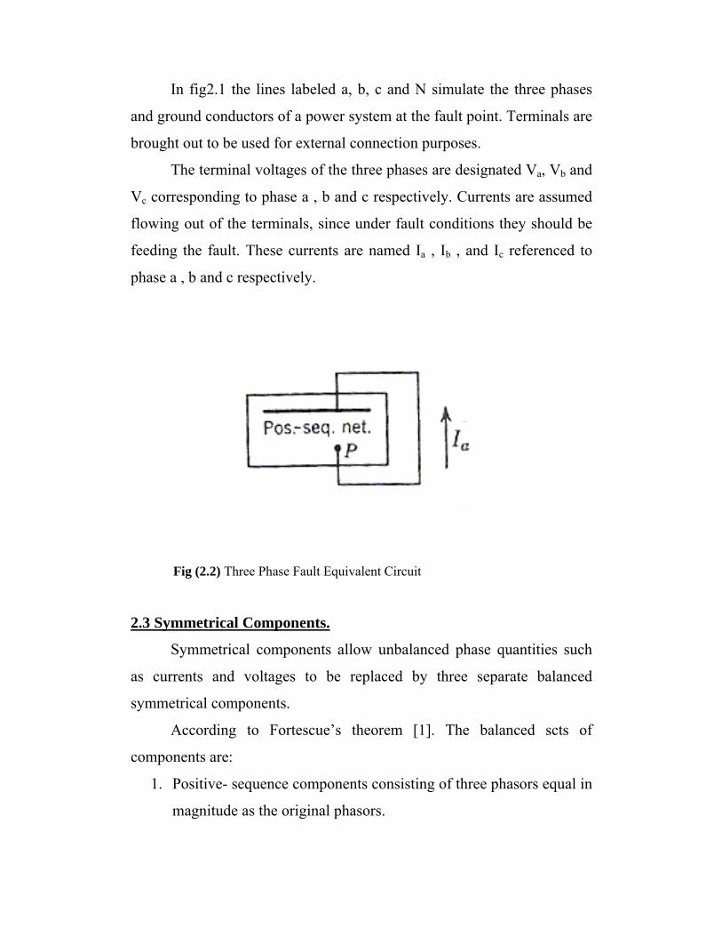
In fig2.1 the lines labeled a, b, c and N simulate the three phases

and ground conductors of a power system at the fault point. Terminals are

brought out to be used for external connection purposes.

The terminal voltages of the three phases are designated Va, Vb and

Vc corresponding to phase a , b and c respectively. Currents are assumed

flowing out of the terminals, since under fault conditions they should be

feeding the fault. These currents are named Ia , Ib , and Ic referenced to

phase a , b and c respectively.

Fig (2.2) Three Phase Fault Equivalent Circuit

2.3 Symmetrical Components.

Symmetrical components allow unbalanced phase quantities such

as currents and voltages to be replaced by three separate balanced

symmetrical components.

According to Fortescue’s theorem [1]. The balanced scts of

components are:

1. Positive- sequence components consisting of three phasors equal in

magnitude as the original phasors.

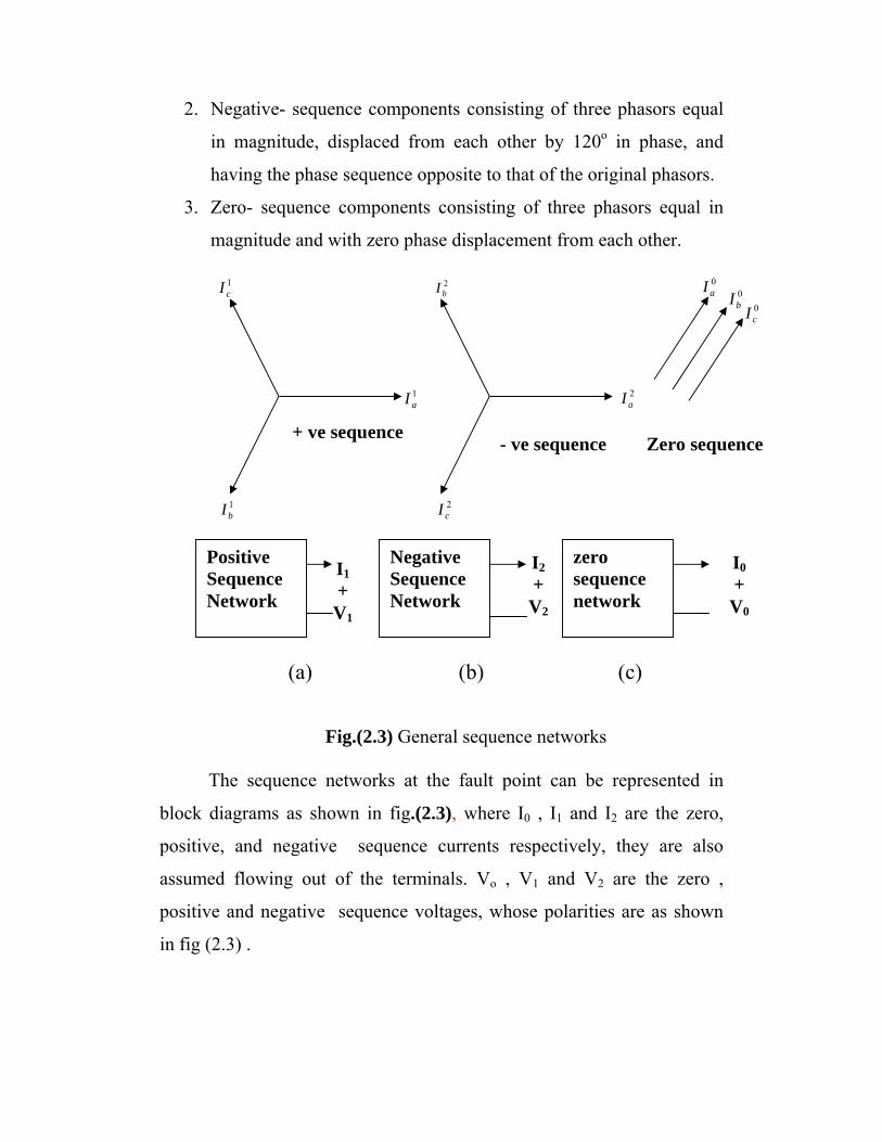
2. Negative- sequence components consisting of three phasors equal

in magnitude, displaced from each other by 120o in phase, and

having the phase sequence opposite to that of the original phasors.

3. Zero- sequence components consisting of three phasors equal in

magnitude and with zero phase displacement from each other.

Fig.(2.3) General sequence networks

The sequence networks at the fault point can be represented in

block diagrams as shown in fig.(2.3), where I0 , I1 and I2 are the zero,

positive, and negative sequence currents respectively, they are also

assumed flowing out of the terminals. Vo , V1 and V2 are the zero ,

positive and negative sequence voltages, whose polarities are as shown

in fig (2.3) .

1cI

1bI

1aI

2bI

2cI

2aI

0aI 0

bI0cI

zero sequence network

Positive Sequence Network

Negative Sequence Network

I0 + V0

I1 + V1

I2 + V2

+ ve sequence - ve sequence Zero sequence

(a) (b) (c)

It should be noted that all three sequence networks are passive

except the positive sequence network which can be reduced to a voltage

source in series with the positive sequence impedance.

The general behavior of the system under fault condition may be

analyzed by proper interconnection between the sequence models.

By convention, the direction of rotation of the phasors is taken to be

counterclockwise. The three phasors are written as [3]

1a

11

1a

211

1a

11

I a 120

I a 240

I 0

=∠=

=∠=

=∠=

oac

oab

oaa

II

II

II

… (2.1)

where we have defined an operator a that causes a counterclockwise

rotation of 120o, such that

joIa

joIajoIa

+=∠=

−−=∠=

+−=∠=

1360866.5.0240

866.5.0120

03

02

0

… (2.2)

From above, it is clear that

01 2 =++ aa … (3-3)

The order of the phasors is abc. This is designated the positive phase

sequence. When the order is abc as in Figure 10.1(b), it is designated the

negative phase sequence. The negative phase sequence quantities are

represented as

2a

222

2a

22

2a

22

I a 240

I a 120

I 0

=∠=

=∠=

=∠=

oac

oab

oaa

II

II

II

… (2.4)

when analyzing certain types of unbalanced faults, it will be found that a

third set of balanced phasors must be introduced. These phasors, known

as the zero phase sequence, are found to be in phase sequence currents, as

in Figure (2.3), would be designated

000cba III == … (2.5)

Consider the three- phase unbalanced currents Ia, Ib, and Ic fig23. .

The three symmetrical components of the current such that

210

210

210

cccc

bbbb

aaaa

IIII

IIII

IIII

++=

++=

++=

… (2.6)

According to the definition of the symmetrical components as given by

(2.1), (2.4), we can rewrite (2.6) all in terms of phase a components.

2210

2120

210

aaac

aaab

aaaa

IaaIII

aIIaII

IIII

++=

++=

++=

… (2.7)

or

⎥⎥⎥

⎦

⎤

⎢⎢⎢

⎣

⎡

⎥⎥⎥

⎦

⎤

⎢⎢⎢

⎣

⎡=

⎥⎥⎥

⎦

⎤

⎢⎢⎢

⎣

⎡

2

1

0

2

2 11

111

a

a

a

c

b

a

III

aaaa

III

… (2.8)

The above equation can be written in matrix notation as

012 aabc IAI = … (2.9)

Where A is known as symmetrical components transformation matrix

(SCTM), which transforms phasor currents abcI into component currents 012aI , and is

⎥⎥⎥

⎦

⎤

⎢⎢⎢

⎣

⎡=

2

2

11

111

aaaaA … (2.10)

Solving (2.9) for the symmetrical components of currents, have

1012 abca IAI −= … (2.11)

The inverse of A is given by

⎥⎥⎥

⎦

⎤

⎢⎢⎢

⎣

⎡=−

aaaaA

2

21

11

111

31 … (2.12)

From (2.10) and (2.12), conclude that

•− = AA311 … (2.13)

A* is the conjugate of A

Substituting from A-1 in (10.11), we have

⎥⎥⎥

⎦

⎤

⎢⎢⎢

⎣

⎡

⎥⎥⎥

⎦

⎤

⎢⎢⎢

⎣

⎡=

⎥⎥⎥

⎦

⎤

⎢⎢⎢

⎣

⎡

c

b

a

a

a

a

III

aaaa

III

11

111

31

2

2

2

1

0

… (2.14)

or in component form, the symmetrical components are

)(31

)(31

)(31

22

21

0

cbaa

cbaa

cbaa

aIIaII

IaaIII

IIII

++=

++=

++=

… (2.15)

From (2.15), the zero- sequence component of current is equal to

one- third of sum of the phase currents. Therefore, when the phase

currents sum to zero, e.g, in a three- phase system with ungrounded

neutral, the zero- sequence current cannot exist. If the neutral of the

power system is grounded, zero-sequence current flows between the

neutral and the ground.

Similar expressions exist for voltages. Thus the unbalanced phase

voltages in terms of the symmetrical components voltages are

2210

2120

210

aaac

aaab

aaaa

VaaVVV

aVVaVV

VVVV

++=

++=

++=

… (2.16)

or in matrix notation

abcVAV 1012 −= … (2.17)

The symmetrical components in terms of the unbalanced voltages are

)(31

)(31

)(31

22

21

0

cbaa

cbaa

cbaa

aVVaVV

VaaVVV

VVVV

++=

++=

++=

… (2.18)

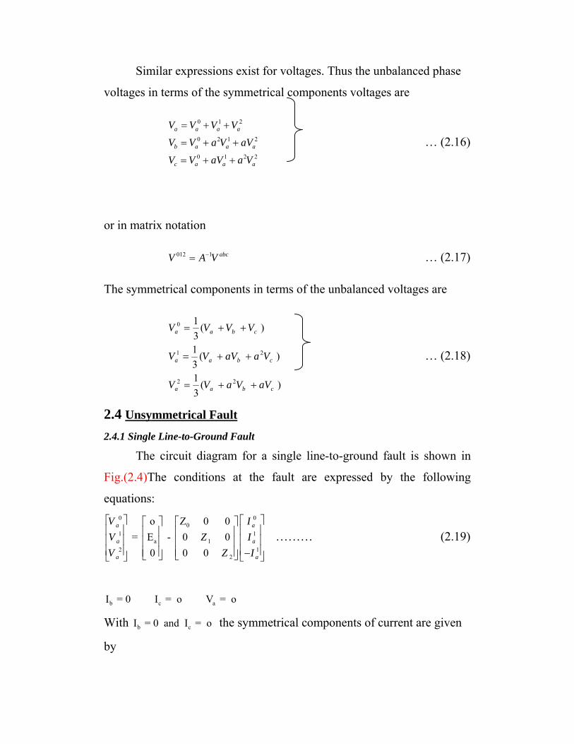
2.4 Unsymmetrical Fault 2.4.1 Single Line-to-Ground Fault

The circuit diagram for a single line-to-ground fault is shown in

Fig.(2.4)The conditions at the fault are expressed by the following

equations: 0 0

01 1

a 12 1

2

o Z 0 0 = E - 0 0

0 0 0

a a

a a

a a

V IV Z IV Z I

⎡ ⎤ ⎡ ⎤⎡ ⎤ ⎡ ⎤⎢ ⎥ ⎢ ⎥⎢ ⎥ ⎢ ⎥⎢ ⎥ ⎢ ⎥⎢ ⎥ ⎢ ⎥⎢ ⎥ ⎢ ⎥⎢ ⎥ ⎢ ⎥ −⎣ ⎦ ⎣ ⎦⎣ ⎦ ⎣ ⎦

……… (2.19)

b c aI = 0 I = o V = o

With b cI = 0 and I = o the symmetrical components of current are given

by

0a

1 2

2 2

1 1 1 I1 = 1 03

1 0

a

a

a

II a aI a a

⎡ ⎤ ⎡ ⎤ ⎡ ⎤⎢ ⎥ ⎢ ⎥ ⎢ ⎥⎢ ⎥ ⎢ ⎥ ⎢ ⎥⎢ ⎥ ⎢ ⎥ ⎢ ⎥⎣ ⎦ ⎣ ⎦⎣ ⎦

so that aoI for 1aI and 2aI each equal aI /3 and 1 2 0 = = a a aI I I … (2.20)

Substituting 1aI for 2aI and aoI in Eq. (2.19), obtain 0 1

01 1

a 12 1

2

o Z 0 0 = E - 0 0

0 0 0

a a

a a

a a

V IV Z IV Z I

⎡ ⎤ ⎡ ⎤⎡ ⎤ ⎡ ⎤⎢ ⎥ ⎢ ⎥⎢ ⎥ ⎢ ⎥⎢ ⎥ ⎢ ⎥⎢ ⎥ ⎢ ⎥⎢ ⎥ ⎢ ⎥⎢ ⎥ ⎢ ⎥⎣ ⎦ ⎣ ⎦⎣ ⎦ ⎣ ⎦

… (2.21)

0 1 2 1 1 1

0 1 2 a a a a a a aV V V I Z E I Z I Z+ + = − + − − … (2.22)

Since 0 1 2

a = + V 0a a aV V V+ =

1

1 2

aa

o

EIZ Z Z

=+ +

… (2.23)

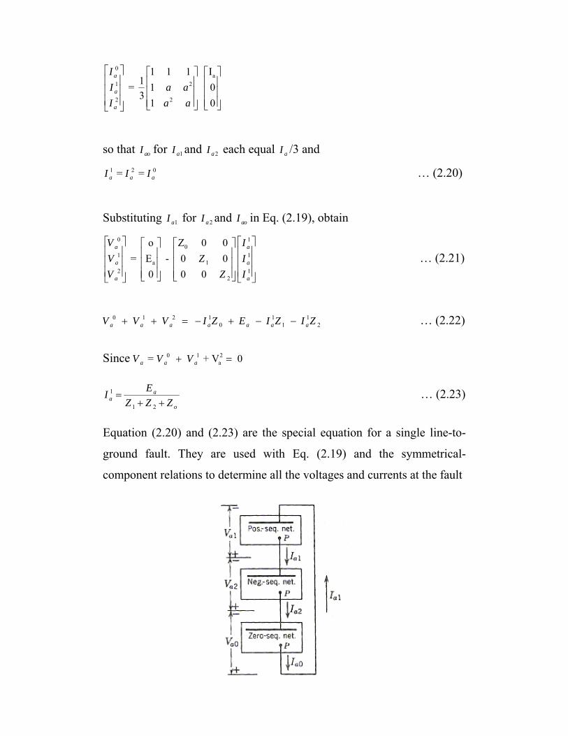
Equation (2.20) and (2.23) are the special equation for a single line-to-

ground fault. They are used with Eq. (2.19) and the symmetrical-

component relations to determine all the voltages and currents at the fault

Fig (2.4) Single Line – to – ground fault

2.4.2 Line-to-Line Fault The circuit diagram for a line-to-line fault is shown in Fig.(2.4) The

conditions at the fault are expressed by the following equations:

a b I 0 Ib c cV V I= = =

With b cV V= the symmetrical components of voltage are given by 0

a1 2

b2 2

b

1 1 1 V1 1 V3

1 V

a

a

a

VV a aV a a

⎡ ⎤ ⎡ ⎤ ⎡ ⎤⎢ ⎥ ⎢ ⎥ ⎢ ⎥=⎢ ⎥ ⎢ ⎥ ⎢ ⎥⎢ ⎥ ⎢ ⎥ ⎢ ⎥⎣ ⎦ ⎣ ⎦⎣ ⎦

from which find

1 2a aV V= … (2.24)

Since 0b c aI I and I= − = , the symmetrical components of current are

given by

1 2

2 2

0 1 1 1 01 13

1a c

a c

I a a II a a I

⎡ ⎤ ⎡ ⎤ ⎡ ⎤⎢ ⎥ ⎢ ⎥ ⎢ ⎥= −⎢ ⎥ ⎢ ⎥ ⎢ ⎥⎢ ⎥ ⎢ ⎥ ⎢ ⎥⎣ ⎦ ⎣ ⎦ ⎣ ⎦

and therefore

0 0aI = … (2.25)

2 1a aI I= − … (2.26)

0 0aV = … (2.27)

since 0aI is zero by Eq. (2.25).

equation (2.19), with the substitutions allowed by Eqs. (2.25) to

(2.27), becomes

0

1 11

2 02

0 0 0 0 00 0

0 0 0a a a

a a

ZV E Z IV Z I

⎡ ⎤ ⎡ ⎤ ⎡ ⎤ ⎡ ⎤⎢ ⎥ ⎢ ⎥ ⎢ ⎥ ⎢ ⎥= −⎢ ⎥ ⎢ ⎥ ⎢ ⎥ ⎢ ⎥⎢ ⎥ ⎢ ⎥ ⎢ ⎥ ⎢ ⎥−⎣ ⎦ ⎣ ⎦ ⎣ ⎦ ⎣ ⎦

…(2.28)

Performing the indicated matrix operations and premultiplying the

resulting matrix equation by the row matrix [ 1 1 -1 ] gives

1 11 20 a a aE I Z I Z= − − … (2.29)

and solving for 1aI yields

1

1 2

aa

EIZ Z

=+

… (2.30)

Equation (2.24),(2.26) and (2.30) are the special equation for a single

line-to-ground fault. They are used with Eq. (2.19) and the symmetrical-

component relations to determine all the voltages and currents at the fault

Fig.(2.5) line – to – line fault 2.4.3Double Line-to-Ground Fault The circuit diagram for a double line-to-ground fault is shown in Fig.(2.5)

the conditions at the fault are expressed by the following equations:

1c0 V 0 IbV o= = =

With c0 and V 0bV = = the symmetrical of voltage are given by

0a

1 2

2 2

1 1 1 V1 = 1 03

1 0

a

a

a

VV a aV a a

⎡ ⎤ ⎡ ⎤ ⎡ ⎤⎢ ⎥ ⎢ ⎥ ⎢ ⎥⎢ ⎥ ⎢ ⎥ ⎢ ⎥⎢ ⎥ ⎢ ⎥ ⎢ ⎥⎣ ⎦ ⎣ ⎦⎣ ⎦

Therefore 0, a1 a2 a V , and V equal V / 3,aV and

1 2 0a a aV V V= = … (2.31)

Substituting 1 1 01 ,a a a aE I Z for V V− and 0aV in Eq. (2.19) and

multiplying both sides by Z-1, where

-1 00

11

12

2

1 0 0Z

0 010 0 = 0 0 Z

0 010 0

ZZ Z

Z

Z

−

⎡ ⎤⎢ ⎥⎢ ⎥⎡ ⎤⎢ ⎥⎢ ⎥= ⎢ ⎥⎢ ⎥⎢ ⎥⎢ ⎥⎣ ⎦ ⎢ ⎥⎢ ⎥⎣ ⎦

give

1 00 0a 1

1 1a 1 a

1 11 2a 1

2 2

1 10 0 0 0Z Z

E 01 1= 0 0 E = 0 0 EZ Z

E 01 10 0 0 0

a a

a a

a a

I Z II Z II Z I

Z Z

⎡ ⎤ ⎡ ⎤⎢ ⎥ ⎢ ⎥⎢ ⎥ ⎢ ⎥⎡ ⎤ ⎡ ⎤− ⎡ ⎤⎢ ⎥ ⎢ ⎥⎢ ⎥ ⎢ ⎥⎢ ⎥− −⎢ ⎥ ⎢ ⎥⎢ ⎥ ⎢ ⎥⎢ ⎥⎢ ⎥ ⎢ ⎥⎢ ⎥ ⎢ ⎥⎢ ⎥− ⎣ ⎦⎣ ⎦ ⎣ ⎦⎢ ⎥ ⎢ ⎥⎢ ⎥ ⎢ ⎥⎣ ⎦ ⎣ ⎦

… (2.32)

Per multiplying both sides of Eq. (2.32) by the row matrix [1 1 1] and

recognizing that 1 2 0 0,a a a aI I I I+ + = = we have

1 1 11 1

0 0 1 2 2 1

a a a aa a a

E E E EZ ZI I IZ Z Z Z Z Z

− + − + − = … (2.33)

and upon collecting terms btain

1 2 01 1

0 2 2 0

( )1 aa

E Z ZZ ZIZ Z Z Z

⎛ ⎞ ++ + =⎜ ⎟

⎝ ⎠ … (2.34)

and 1 2 0

1 2 1 0 2 0 1 2 0 2 0)

( )/(

a aa

E Z Z EIZ Z Z Z Z Z Z Z Z Z Z

+= =

+ + + + … (2.35)

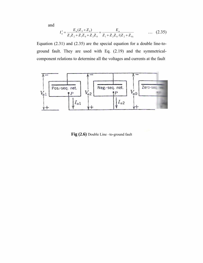
Equation (2.31) and (2.35) are the special equation for a double line-to-

ground fault. They are used with Eq. (2.19) and the symmetrical-

component relations to determine all the voltages and currents at the fault

Fig (2.6) Double Line –to-ground fault

2.5 Zero-sequence equivalent circuits

Three-phase transformer ,together with diagrams of connections and the

symbols for one-line diagrams are shown in fig 2.7 [1]

.

Fig (2.7) Zero-sequence equivalent circuits

Power System Fault Analysis Using Computer

Program

3.1 Introduction

Early before the invention of computers and microprocessors, fault

analysis was obtained by solving large networks, which have large

network equations, formatted by hand or slide ruler. The mathematical

calculations involved were tedious and time consuming. Nowadays after

invention of the computer sand electronic programming, packages of

computational methods were used for the solution of large equations and

power engineering problems which concern matrix technique, load flow

analysis, short circuit studies and power system stability.

For power system to be practical it must be safe, reliable and

economical thus many analyses must be performed to design and operate

an electrical system. However, before going to system analysis we have

to model all components of electrical power system. Design of a power

system, its operation and expansion requires much analysis. This research

presents methods of power system analysis with the aid of personal

computer and the use of MATLAP [3]. The MATLAP environment

permits a direct transition from mathematical expression to simulation.

3.2What Is MATLAB?

MATLAB is a high-performance language for technical

computing. It integrates computation, visualization, and programming in

an easy-to-use environment where problems and solutions are expressed

in familiar mathematical notation. Typical uses include [11]

• Math and computation

• Algorithm development

• Data acquisition

• Modeling, simulation, and prototyping

• Data analysis, exploration, and visualization

• Scientific and engineering graphics

• Application development, including graphical user interface

building

MATLAB is an interactive system whose basic data element is an

array that does not require dimensioning. This allows you to solve many

technical computing problems, especially those with matrix and vector

formulations, in a fraction of the time it would take to write a program in

a scalar noninteractive language such as C or Fortran.

The name MATLAB stands for matrix laboratory. MATLAB was

originally written to provide easy access to matrix software developed by

the LINPACK and EISPACK projects. Today, MATLAB engines

incorporate the LAPACK and BLAS libraries, embedding the state of the

art in software for matrix computation.

MATLAB has evolved over a period of years with input from

many users. In university environments, it is the standard instructional

tool for introductory and advanced courses in mathematics, engineering,

and science. In industry, MATLAB is the tool of choice for high-

productivity research, development, and analysis.

MATLAB features a family of add-on application-specific

solutions called toolboxes. Very important to most users of MATLAB,

toolboxes allow you to learn and apply specialized technology. Toolboxes

are comprehensive collections of MATLAB functions (M-files) that

extend the MATLAB environment to solve particular classes of

problems. Areas in which toolboxes are available include signal

processing, control systems, neural networks, fuzzy logic, wavelets,

simulation, and many others.

3.2.1The MATLAB System. The MATLAB system consists of five

main parts [11]:

a- Development Environment. This is the set of tools and facilities that

help you use MATLAB functions and files. Many of these tools are

graphical user interfaces. It includes the MATLAB desktop and

Command Window, a command history, an editor and debugger, and

browsers for viewing help, the workspace, files, and the search path.

b- The MATLAB Mathematical Function Library. This is a vast

collection of computational algorithms ranging from elementary

functions, like sum, sine, cosine, and complex arithmetic, to more

sophisticated functions like matrix inverse, matrix eigenvalues, Bessel

functions, and fast Fourier transforms.

c- The MATLAB Language. This is a high-level matrix/array language

with control flow statements, functions, data structures, input/output, and

object-oriented programming features. It allows both "programming in

the small" to rapidly create quick and dirty throw-away programs, and

"programming in the large" to create large and complex application

programs.

d- Graphics. MATLAB has extensive facilities for displaying vectors

and matrices as graphs, as well as annotating and printing these graphs. It

includes high-level functions for two-dimensional and three-dimensional

data visualization, image processing, animation, and presentation

graphics. It also includes low-level functions that allow you to fully

customize the appearance of graphics as well as to build complete

graphical user interfaces on your MATLAB applications.

e-The MATLAB Application Program Interface (API). This is a

library that allows you to write C and Fortran programs that interact with

MATLAB. It includes facilities for calling routines from MATLAB

(dynamic linking), calling MATLAB as a computational engine, and for

reading and writing MAT-files.

Some of analysis covered in this study are:

- Balanced fault

- Symmetrical components and unbalanced fault

- Stability studies.

3.3 Z-Impedance Building And Symmetrical fault Programs

Two functions are developed for the formation of the bus impedance

matrix .One function is named Zbus=zbus(zdata) ,where zdata is

an e x 4 matrix containing the impedance data or an e-element network

.Columns 1 and 2 are represent the element bus numbers and columns 3

and 4 contains the element resistance and reactance , respectively, in per

unit. Bus number 0 to generator buses contain generator impedances

.These may be the subtransient , transient, or synchronous reactances .

Also any other shunt impedances such as capacitors and load impedance

to ground (bus 0) may be included in this matrix.

The other function for the formation of the bus impedance matrix is zbus

=zbuildpi(linedata, gendata ,yload), which is compatible with the

power flow programs . The first argument linedata is consistent with the

data required for the power flow solution .Columns 1 and 2 are the line

bus numbers. Columns 3 through 5 contain line resistance , reactance, and

one-half of the total line charging susceptance in per unit on the specified

MVA base .The last column is for the transformer tap setting ;for lines, 1

must be entered in this column .The lines may be entered in any sequence

or order .The generator reactances are not included in the linedata of the

power flow program and must be specified separately as required by the

gendata in the second argument .gendata is an ngx4 matrix ,where each

row contains bus 0, generator bus number ,resistance and reactance .The

last argument, yload is optional. This is a two-column matrix containing

bus number and the complex load admittance .This data is provided by

any of the power flow programs ifgauss, ifnewton or decouple .yload is

automatically generated following the execution of any of the above

power flow programs.

The zbuild and zbuildpi functions used to obtained the bus impedance

matrix by the building algorithm method. These functions select a tree

containing elements to the reference node.First,all branches connected to

the reference node are processed .Then the remaining branches of the tree

are connected , and finally the cotree links are added.

The program symfault (zdata,Zbus, V) is developed for the

balanced three phase fault studies. The function requires the zdata and

Zbus matrixes. The third argumentV is optional .If it is not included , the

program sets all the prefault bus voltages to 1.0 per unit .If the variable V

is included, the prefault bus voltages must be specified by the array V

containing bus numbers and the complex bus voltage. The voltage vector

V is automatically generated following the execution or any of the power

flow programs .The use of the above functions are demonstrated in the

following examples .When symfault is executed ,it prompts the user to

enter the faulted bus number and the fault impedance . The program

computes the total fault currents and tabulates the magnitude of the bus

voltages and line currents during the fault .

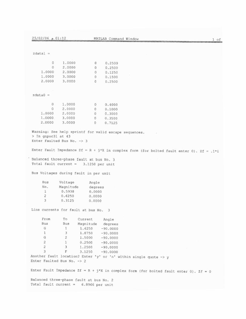
3.3.1Testing the Program[3]

The above discussed program was tested using printed example given in

[3]

A three-phase fault with a fault impedance fZ =j0.1per unit occurs at bus 3

in the network (fig 3.1) .Use the symfault function to compute the fault

current, the bus voltages and line currents during the fault .All shunt

capacitances and loads are neglected and all the prefault bus voltages are

assumed to be unity .The impedance diagram is described by the variable

zdata.

The program codes and the results are shown in Appendix B .The results

of the program was found to be exactly as that found in the

reference[3].

(a)The one line diagram for program

Fig 3.1

(b) (c)

Fig(3.1) (b) Thevenin’s equivalent network,(c)Reduction of thevenin’s network

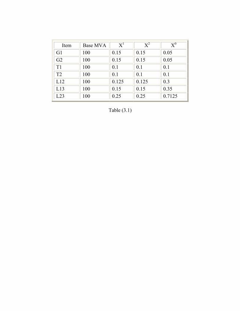
Item Base MVA X1 X2 X0 G1 100 0.15 0.15 0.05 G2 100 0.15 0.15 0.05 T1 100 0.1 0.1 0.1 T2 100 0.1 0.1 0.1 L12 100 0.125 0.125 0.3 L13 100 0.15 0.15 0.35 L23 100 0.25 0.25 0.7125

Table (3.1)

3.4 Symmetrical Components Programs

Transformation from phase quantities to symmetrical components in

MATLAP is very easy. Once the symmetrical components

transformation matrix A is defined, its inverse is found using the

MATLAP function inv. However, for quick calculations and graphical

demonstration, the following functions are developed for symmetrical

components analysis.

Sctm The symmetrical components transformation matrix A is defined in

this script file . Typing sctm defines A.

Phasor(F) This function makes plots of phasors. The variable F maybe

expressed in an n x 1 array in rectangular complex form or as an n x 2

matrix . In the latter case , the first column is the phasor magnitude and

the second column is its phase angle in degree.

F012=abc2sc(Fabc)This function returns the symmetrical components of

a set of unbalanced phasors in rectangular form. Fabc may be expressed

in 3 x 1 array in rectangular complex form or as a 3 x 2 matrix .In the

latter case ,the first column is the phasor magnitude and the second

column is its phase angle in degree for a, b, and c phases. In addition, the

function produces aplot of the unbalanced phasors and its symmetrical

components.

Fabc=sc2abc(F012)This function returns the unbalanced phasors in

rectangular form when symmetrical components are specified .F012 may

be expressed in a 3 x 1 array in rectangular complex form or as a 3 x 2

matrix. In the latter case, the first column is the phasor magnitude and

the second column is its phase angle in degree for the zero-,positive -, and

negative –sequence components, respectively. In addition, the function

produces a plot of the unbalanced phasors and its symmetrical

components.

012 2 ( )Z zabc sc Zabc= This function transforms phase impedance matrix to

the sequence impedance matrix.

2 ( )Fp rec pol Ft= This function converts the rectangular phasor Ft into

polar form Fp .

2 ( )Ft pol rec Fp= This function converts the polar phasor Fp into

rectangular form Fr .

3.4.1Testing the Program [3]

The above discussed program was tested using printed example given in

[3]

Obtain the symmetrical components of a set of unbalanced currents

Ia = 1.6 25,Ib = 1.0 180 , and Ic =.9 132 .Iabc = [1.6 25 1.0 180 .9 132];

∠∠ ∠

I012 = abc2sc(Iabc);% Symmetrical components of phase a

I012p= rec2pol(I012) % Converts rectangular phasors into polar form

I012p =

Result in

0.4512 96.4529 0.9435 -0.0550 0.6024 22.3157

-1 0 1

-1

0

1

a-b-c set

-1 0 1

-1

0

1

Zero-sequence set

-1 0 1

-1

0

1

Positive-sequence set

-1 0 1

-1

0

1

Negative-sequence set

Fig (3.2) Transformation of the symmetrical components into phasor components.

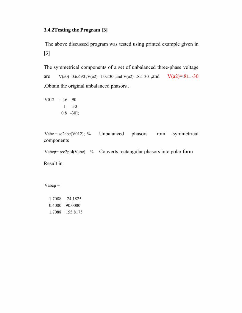
3.4.2Testing the Program [3]

The above discussed program was tested using printed example given in

[3]

The symmetrical components of a set of unbalanced three-phase voltage

are V(a0)=0.6 90 ,V(a2)=1.0 30 ,and V(a2)=.8 -30 ∠ ∠ ∠ ,and V(a2)=.8∟-30

.Obtain the original unbalanced phasors .

V012 = [.6 90 1 30 0.8 -30];

Vabc = sc2abc(V012); % Unbalanced phasors from symmetrical components

Vabcp= rec2pol(Vabc) % Converts rectangular phasors into polar form

Result in

Vabcp =

1.7088 24.1825 0.4000 90.0000 1.7088 155.8175

-1 0 1

-1

0

1

a-b-c set

-1 0 1

-1

0

1

Zero-sequence set

-1 0 1

-1

0

1

Positive-sequence set

-1 0 1

-1

0

1

Negative-sequence set

Fig (3.3) Transformation of the symmetrical components into phasor components.

3.5 Unbalanced Fault Programs

Three function are developed for the unbalanced fault analysis.These

functions are lgfault(zdata0,Zbus0,zdata1,Zbus1,zdata2,Zbus2,V)

llfault(zdata1,Zbus1,zdata2,Zbus2,V),anddlgfault(zdata0,Zbus0,zdat

a1,Zbus1,zdata2,Zbus2,V). lgfault is designed for the single line –to-

ground fault analysis ,llfault for the line-to-line fault analysis, and

dlgfault for the double line to ground fault analysis of a power system

network. Lgfault and dlgfault require the positive –negative-,and zero-

sequence bus impedance matrices Zbus0,Zbus1, andZbus2, and llfault

requires the positive –and negative-sequence bus impedance matrices

Zbus1, and Zbus2.The last argument V is optional .If it is not included,

the program sets all the prefault bus voltages to 1.0 per unit. If the

variable V is included , the prefault bus voltages must be specified by the

array V containing bus numbers and the complex bus voltage. The

voltage vector V is automatically generated following the execution of

any of the power flow programs.

The bus impedance matrices may be obtained from

Zbus0=zbuild(zdata),and Zbus1=zbuild(zdata1).The argument zdata1

contains the positive-sequence network impedances. zdata0 contains the

zero-seqence network impedances .Arguments zdata0, zdata1and

zdata2,are an e x 4matrices containing the impedance data of an e-

element network . Columns 1 and 2 are the element bus numbers and

columns 3 and 4 contain the element resistance reactance, respectively, in

per unit. Bus number 0 to generator buses contains generator impedances.

These may be the sub transient, transient, or synchronous reactance .Also,

any other shunt impedances such as capacitors and load impedances to

ground (bus0) may be included in this matrix.

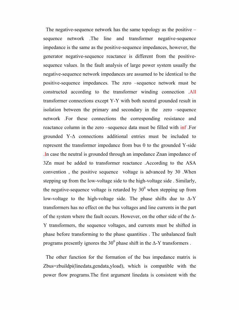
The negative-sequence network has the same topology as the positive –

sequence network .The line and transformer negative-sequence

impedance is the same as the positive-sequence impedances, however, the

generator negative-sequence reactance is different from the positive-

sequence values. In the fault analysis of large power system usually the

negative-sequence network impedances are assumed to be identical to the

positive-sequence impedances. The zero –sequence network must be

constructed according to the transformer winding connection .All

transformer connections except Y-Y with both neutral grounded result in

isolation between the primary and secondary in the zero –sequence

network .For these connections the corresponding resistance and

reactance column in the zero –sequence data must be filled with inf .For

grounded Y-∆ connections additional entries must be included to

represent the transformer impedance from bus 0 to the grounded Y-side

.In case the neutral is grounded through an impedance Znan impedance of

3Zn must be added to transformer reactance .According to the ASA

convention , the positive sequence voltage is advanced by 30 .When

stepping up from the low-voltage side to the high-voltage side . Similarly,

the negative-sequence voltage is retarded by 300 when stepping up from

low-voltage to the high-voltage side. The phase shifts due to ∆-Y

transformers has no effect on the bus voltages and line currents in the part

of the system where the fault occurs. However, on the other side of the ∆-

Y transformers, the sequence voltages, and currents must be shifted in

phase before transforming to the phase quantities . The unbalanced fault

programs presently ignores the 300 phase shift in the ∆-Y transformers .

The other function for the formation of the bus impedance matrix is

Zbus=zbuildpi(linedata,gendata,yload), which is compatible with the

power flow programs.The first argument linedata is consistent with the

data required for the power flow slution . Columns1 and 2 are the line bus

number. Column 3 through 5 contain the line resistance, reactance, and

one-half of the total line charging susceptance in per unit on the specified

MVA base. The last column is for the transformer tap setting; for lines, 1

must be entered in this column. The generator reactances are not included

in the linedata for the power flow program and must be specified

separately as required by gendata in the second argument. gendata is an

eg x 4 , matrix, where each row contains bus o, generator bus number,

resistance and reactance. The last argument yload is optional. This is a

tow-column matrix containing bus number and the complex load

admittance. This data is provided by any of the power flow programs

lfgauss, lfnewton or decouple. Yload is automatically generated following

the execution of the above power flow programs.

The program prompts the user to enter the faulted bus number and the

faulted impedance Zf. The program obtains the total fault current, bus

voltages and line currents during the fault. The use of the above functions

are demonstrated in the following examples.

3.5.1Testing the Program [3]

The above discussed program was tested using printed example given

in [3]

Use the lgfault' llfault, and dlgfault functions to compute the fault

current, bus voltages and line currents the circuit in fig no for the

following fault .

(a)A single-line-to-ground fault at bus 3 through afault impedance

fZ =j0.1per unit .

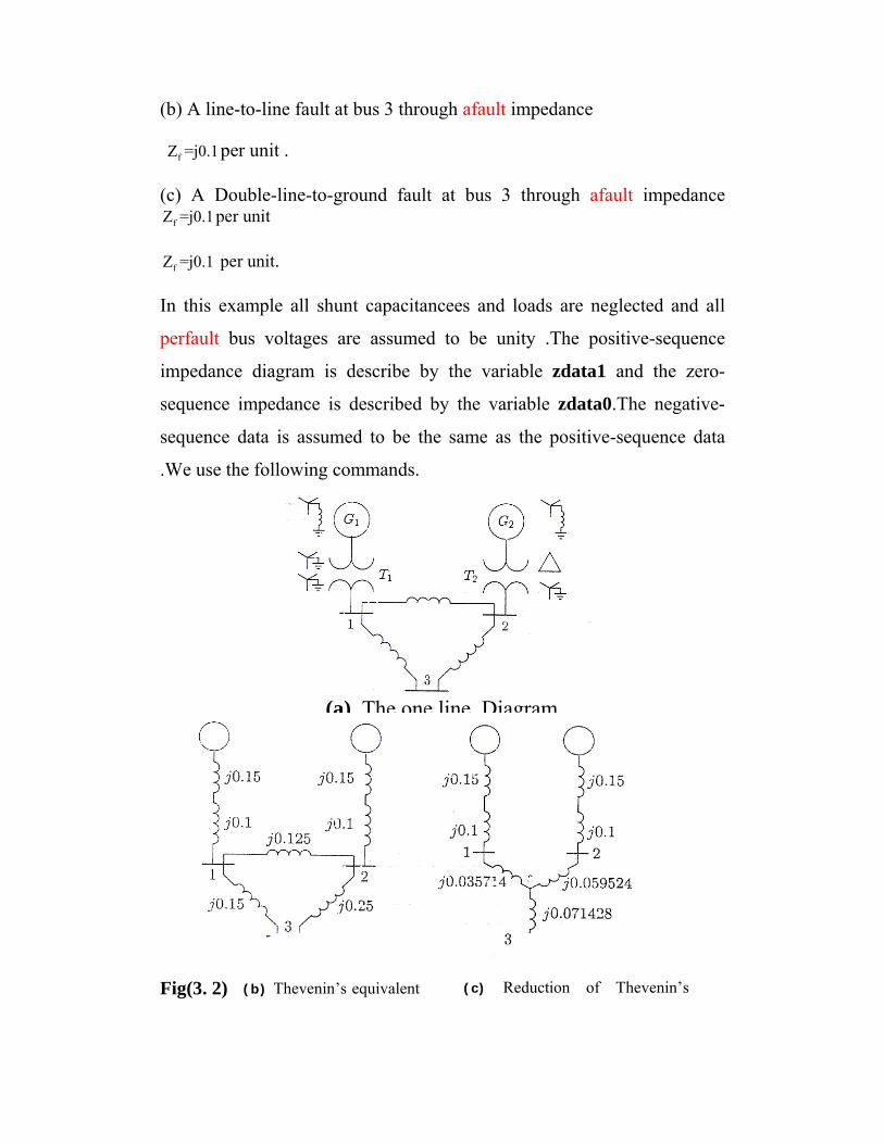
(b) A line-to-line fault at bus 3 through afault impedance

fZ =j0.1per unit .

(c) A Double-line-to-ground fault at bus 3 through afault impedance fZ =j0.1per unit

fZ =j0.1 per unit.

In this example all shunt capacitancees and loads are neglected and all

perfault bus voltages are assumed to be unity .The positive-sequence

impedance diagram is describe by the variable zdata1 and the zero-

sequence impedance is described by the variable zdata0.The negative-

sequence data is assumed to be the same as the positive-sequence data

.We use the following commands.

Fig(3. 2)

(a) The one line Diagram

(b) Thevenin’s equivalent (c) Reduction of Thevenin’s

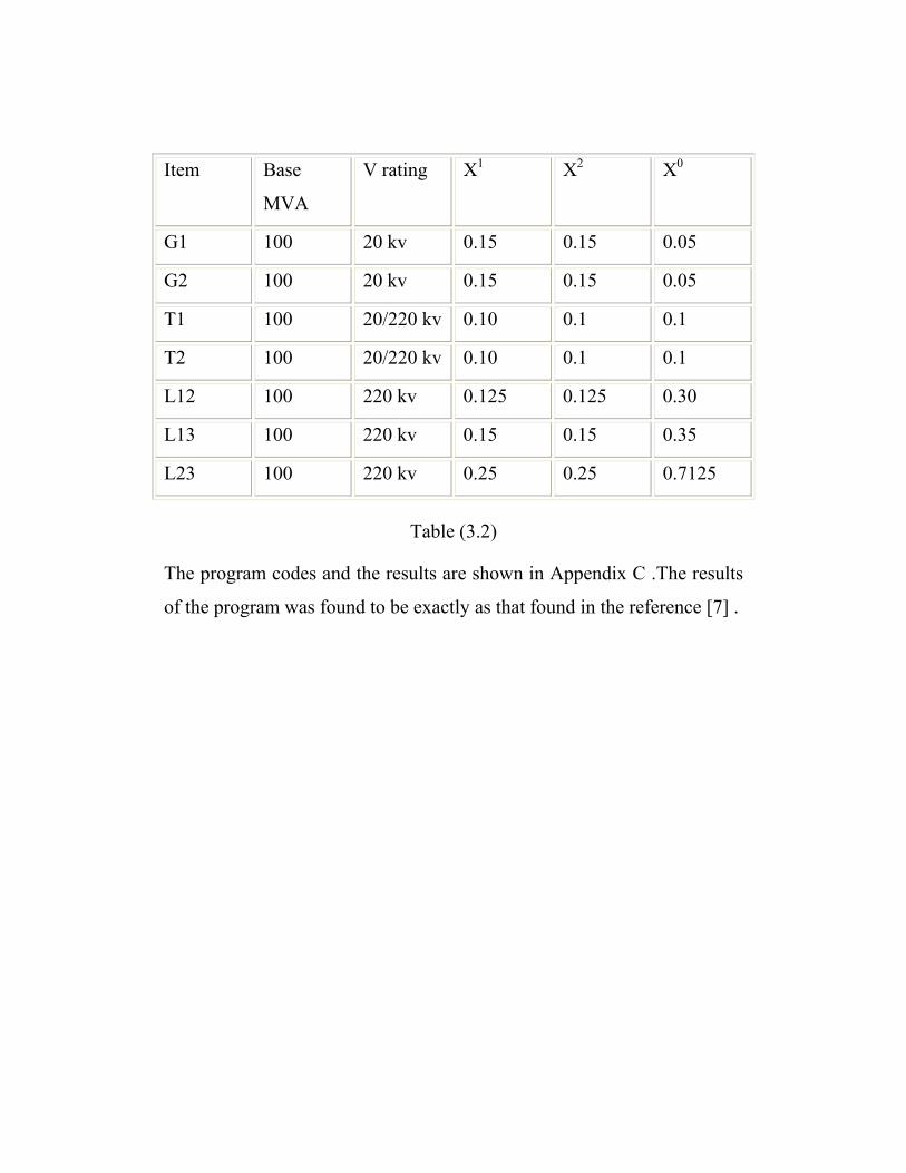
Item Base

MVA

V rating X1 X2 X0

G1 100 20 kv 0.15 0.15 0.05

G2 100 20 kv 0.15 0.15 0.05

T1 100 20/220 kv 0.10 0.1 0.1

T2 100 20/220 kv 0.10 0.1 0.1

L12 100 220 kv 0.125 0.125 0.30

L13 100 220 kv 0.15 0.15 0.35

L23 100 220 kv 0.25 0.25 0.7125

Table (3.2)

The program codes and the results are shown in Appendix C .The results

of the program was found to be exactly as that found in the reference [7] .

3.6 Power Flow Programs: Several computer programs have been developed for the power

flow solution of practical systems. Each method of solution consists of

four programs. The program for the Gauss-Seidel method is lfgauss,

which is preceded by Ifybus, and is a followed by busout and lineflow.

Programs Ifybus, busout, and lineflow are designed to be used with two

more pcwer flow programs. These are ifnewton for the Newton-Raphson

method and decouple for the fast decoupled method. The following is a

brief description of the programs used in the Gauss-Seidel method [3].

(a)Ifybus This program requires the line and transformer parameters and

transformer tap settings specified in the input file named linedata.

It converts impedance to admittance and obtains the bus admittance

matrix. The program is signed to handle parallel lines.

(b)lfgauss This program obtains the power flow solution by the Gauss-

Seidel method and requires the files named busdata and linedata.

It is designed for direct use of load and generation in MW and

Mvar, bus voltages in per unit and angle in degrees. Loads and

generation are converted to per unit quantities on the base MVA

selected. A provision is made to maintain the generator reactive

power of the voltage-controlled buses within their specified limits.

The violation of reactive power limit may occur if the specified

voltage is either too high or too low. After a few iterations (10th

iteration in the Gauss method), the var calculated at the generator

buses are examined. If a limit reached, the voltage magnitude is

adjusted in steps of 0.5 percent up to percent to bring the var

demand within the specified limits .-

(c)busout This program produces the bus output result in a tabulated

form The busout result includes the voltage magnitude and angle

real and reactive power of generators and loads, and the shunt

capacitor/reactor Mvar. Total generator and total load are also

included as outlined in the sample case.

(d)Lineflow This program prepares the line output data. It is

designed to display the active and reactive power flow entering the

line terminals and line losses as well as the net power at each bus.

Also included are the total real and reactive losses in the system.

The output of this portion is also shown in the sample case.

3.6.1 Data Preparation:

In order to perform a power flow analysis by the Gauss-Seidel

method in the MAT-LAP environment, the following variables must be

defined: power system base MVA, power mismatch accuracy,

acceleration factor, and maximum number of iterations. The name (in

lowercase letters) reserved for these variables are basemva, accuracy,

accel, and maxiter, respectively. Typical values ate as follows:

Basemva=100; accuracy=0.001;

Accel=1.6; maxiter=80;

The iinitial step in the preparation of input file is the numbering of each

bus. Buses are numbered sequentially. Although the numbers are

sequentially assigned, the buses need not be entered in sequence. In

addition, the following data files are required.

BUS DATA FILE - busdata The format for the bus entry is chosen to

facilitate the required data for each bus in a single row. The information

required must be included in a matrix called busdata. Column I is the bus

number. Column 2 contains the bus code. Columns 3 anc 4 are voltage

magnitude in per unit and phase angle in degrees. Columns 5 and 6 are

load MW and Mvar. Column 7 through 10 are MW, Mvar, minimum

Mvar and maximum Mvar of generation, in that order. The last column is

the injected Mvar of shunt capacitors. The bus code entered in column 2

is used for identifying load, voltage-controlled, and slack buses as out-

lined below:

This code is used for the slack bus. The only necessary information for

this bus is the voltage magnitude and its phase angle.

This code is used for load buses. The loads are entered positive in

megawatts and megavars. For this bus, initial valtage estimate must be

specified. This is usually 1 and 0 for voltage magnitude and phase angle,

respectively. If voltage magnitude and phase angle for this type of bus are

specified, they will be taken as the initial starting voltage for that bus

instead of a flat start of 1 and 0.This code is used for the voltage-

controlled buses. For this bus, voltage magnitude, real power generation

in megawatts, and the minimum and maximum limits of the megavar

demand must be specified.

LINE DATA FILE — linedata Lines are identified by the node-pair

method. The information required must be included in a matrix called

linedata. Columns I and the line bus numbers. Columns 3 through 5

contain the line resistance, reactance, and one-half of the total line

harging susceptance in per unit on the specified

MVA base. The last column is for the transformer tap sethng; for Lines, 1

must be entered in this column. The lines may be entered in any sequence

or order with the only restriction being that if the entry is a ransforrner,

the left bus number is, assumed to be the tap side of the transformer,

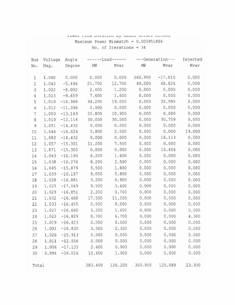
The IEEE 30 bus system is used to demonstrate the data preparation and

the use of the power flow programs by the Gauss-Seidel method.

3.6.2Testing the Program [3]

The above discussed program was tested using printed example given in

[3]

Figure 3.4 is part of the American Electric Power Service Corporation

network which is being made available to the electric utility industry as a

standard test case for evaluating various analytical methods and computer

programs for the solution of power system problems. Use the lfgauss

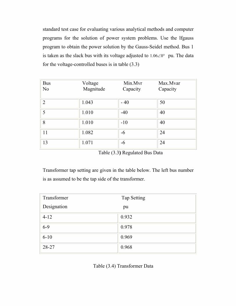
program to obtain the power solution by the Gauss-Seidel method. Bus 1

is taken as the slack bus with its voltage adjusted to 1.06 0° ∠ pu. The data

for the voltage-controlled buses is in table (3.3)

Bus Voltage Min.Mvr Max.Mvar No Magnitude Capacity Capacity

2 1.043 - 40 50

5 1.010 -40 40

8 1.010 -10 40

11 1.082 -6 24

13 1.071 -6 24

Table (3.3) Regulated Bus Data

Transformer tap setting are given in the table below. The left bus number

is as assumed to be the tap side of the transformer.

Transformer Tap Setting

Designation pu

4-12 0.932

6-9 0.978

6-10 0.969

28-27 0.968

Table (3.4) Transformer Data

The data for the injected Q due to shunt capacitors is.

Bus No Mvr

10 19

24 4.3

Table (3.5) Injected Q due to Capacitors

Fig (3.3) American Electric Power Service Corporation Network

IEEE sample system

Generation and loads are as given in the data prepared for use in the

MATLAP environment in the matrix defined as busdata. Code C, code 1,

and code 2 are used for the load buses, the slack bus and the voltage-

controlled buses, respectively. Values for basemva, accuracy, accer and

maxiter must be specified. Line data are as given in the matrix called

linedata. The last column of this data must contain 1 for lines, or the tap

setting values for transformers with off-nominal turn ratio. ‘The control

commands required are Ifybus, lfgauss and lineflow. A diary command

may be used to save the output to the specified file name. The power flow

data and the commands required are as follows.

3.6.3Testing the Program [3]

The above discussed program was tested using printed example given

in [3]

Repeat the symmetrical three-phase short circuit analysis for above

example considering the prefault bus voltages and the effect of load

current. The load data is as follows:

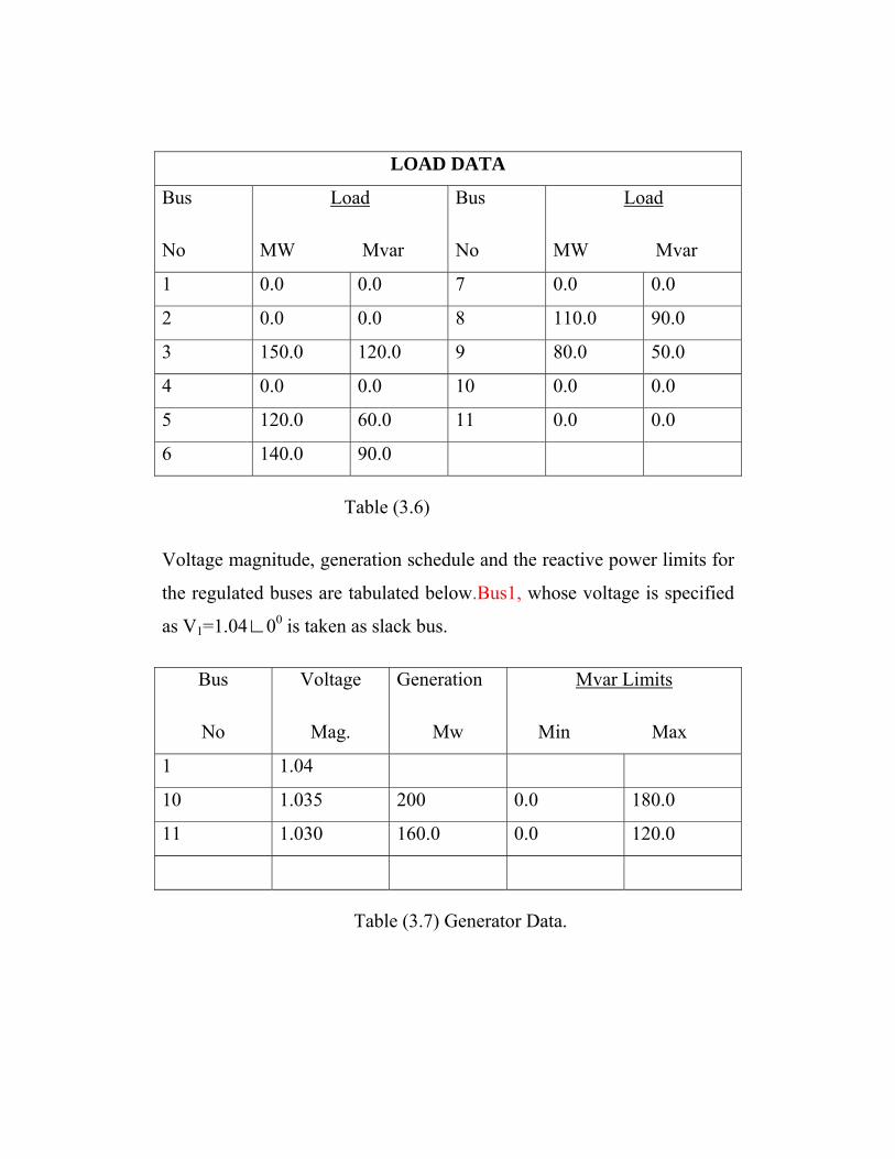
LOAD DATA

Bus

No

Load

MW Mvar

Bus

No

Load

MW Mvar

1 0.0 0.0 7 0.0 0.0

2 0.0 0.0 8 110.0 90.0

3 150.0 120.0 9 80.0 50.0

4 0.0 0.0 10 0.0 0.0

5 120.0 60.0 11 0.0 0.0

6 140.0 90.0

Table (3.6)

Voltage magnitude, generation schedule and the reactive power limits for

the regulated buses are tabulated below.Bus1, whose voltage is specified

as V1=1.04∟00 is taken as slack bus.

Bus

No

Voltage

Mag.

Generation

Mw

Mvar Limits

Min Max

1 1.04

10 1.035 200 0.0 180.0

11 1.030 160.0 0.0 120.0

Table (3.7) Generator Data.

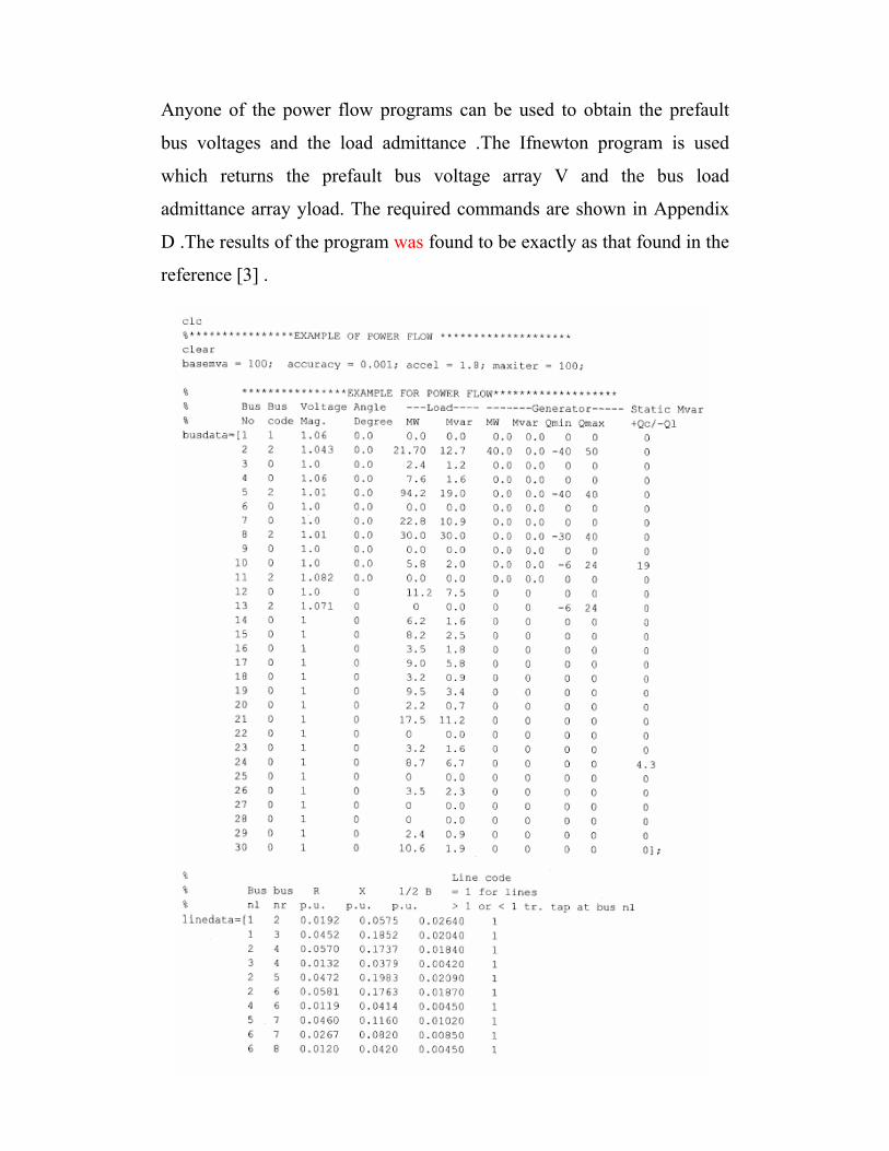
Anyone of the power flow programs can be used to obtain the prefault

bus voltages and the load admittance .The Ifnewton program is used

which returns the prefault bus voltage array V and the bus load

admittance array yload. The required commands are shown in Appendix

D .The results of the program was found to be exactly as that found in the

reference [3] .

GNPOC Network Description and Problems 4.1 Background The Greater Nile Petroleum Operating Company Limited

(GNPOC), Sudan is engaged in oil exploration and production operations

in the area located about 800 kms southwest of Khartoum .Heglig is

located on latitude 29º 23' 73" East ;and longitude10º 00' 48"; North ;and

theUnity field is about 70 kilometers southeast of Heglig. The whole area

falls in the Acacia Seyal “Tall grass savanna zone of the Sudan ".

Fig (4.1) Sudan Oil Map

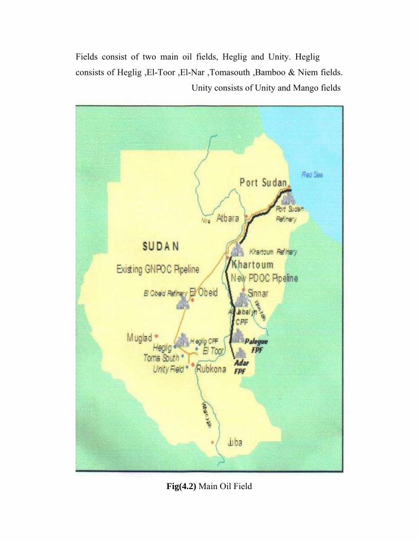
Fields consist of two main oil fields, Heglig and Unity. Heglig

consists of Heglig ,El-Toor ,El-Nar ,Tomasouth ,Bamboo & Niem fields.

Unity consists of Unity and Mango fields

Fig(4.2) Main Oil Field

ComTransm

Fig(4.3) shows the power system from 1999; up to date.

Fig(4.3) power system up to date

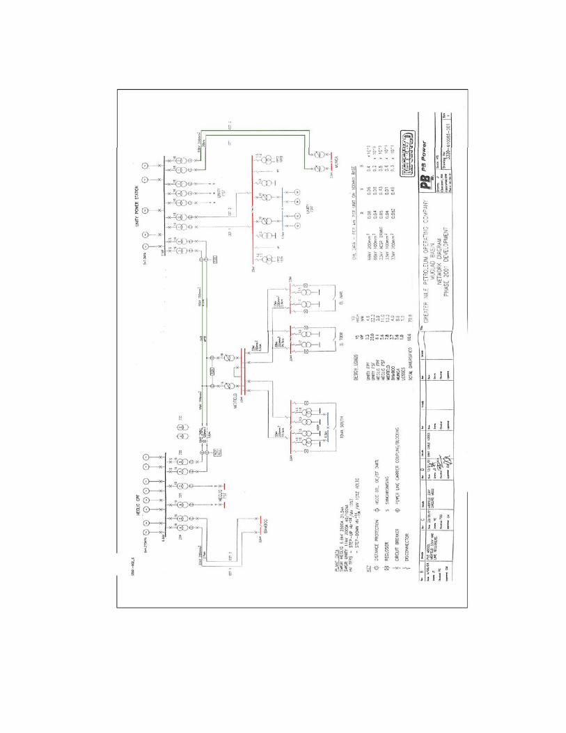
Power System4.2

GNPOC has two captive power plants one at Heglig (HPP) and the other

at Unity (UPP), to cater for the power needs of various oil wells and their

field & central processing facilities. The power generated is transmitted

to the loads at 66 kV & 33 kV voltage levels through overhead and

underground cable Network

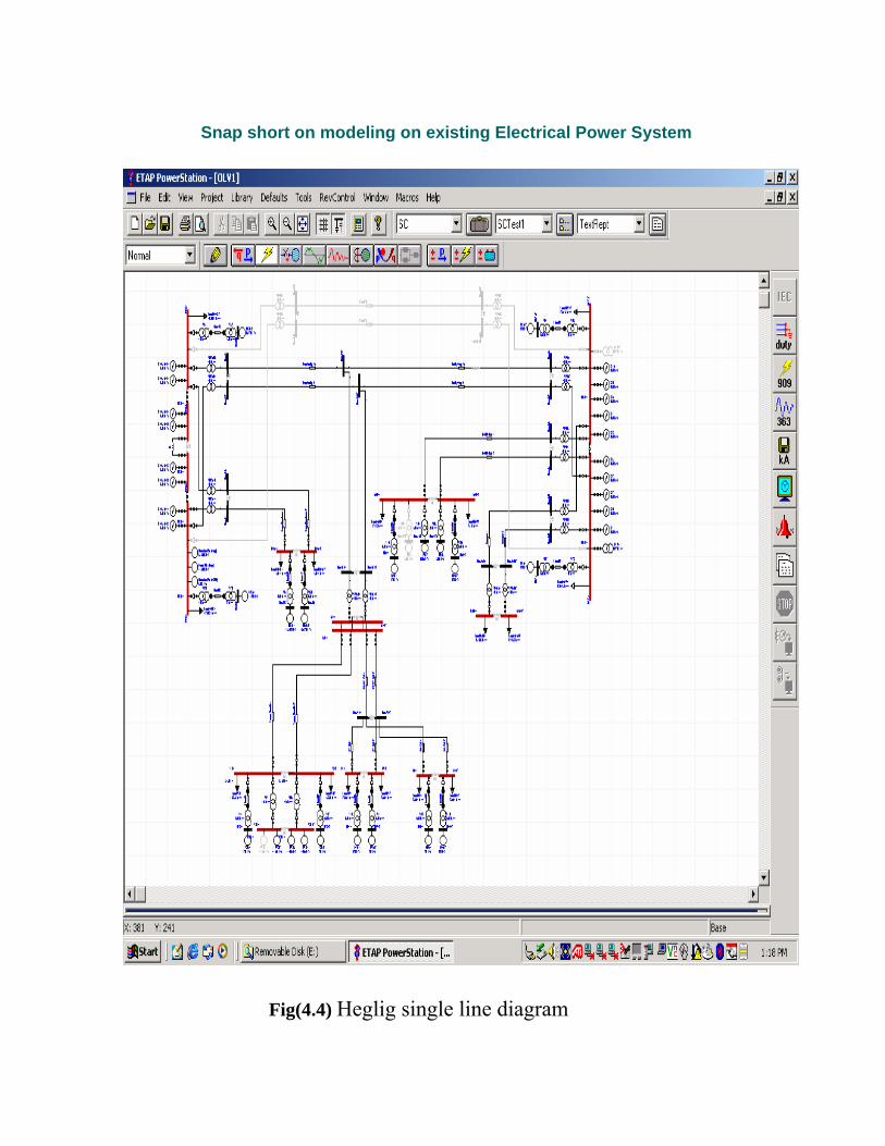
Snap short on modeling on existing Electrical Power System

Fig(4.4)

Fig(4.4) Heglig single line diagram

Started in year 2000, Electrical Power System and Network had drastically expand with the production increased from

150 kbpd to 300 kbpd, demand newHEGLIG POWER PLANT

8 x 3.5MW Generator (Crude Fuel Engine)

:Field Heglig North & Heglig South

:Facilities Field Production Facilities (FPF) &

Field Surface Facilities (FSF)

:Field Toma South, El Nar & El Toor

:Facilities Field Production Facilities (FPF) &

Field Surface Facilities (FSF)

:Field Unity

:Facilities Field Production Facilities (FPF) &

Field Surface Facilities (FSF)

UNITY POWER PLANT 8 x 3.5MW Generator (Crude Fuel Engine)

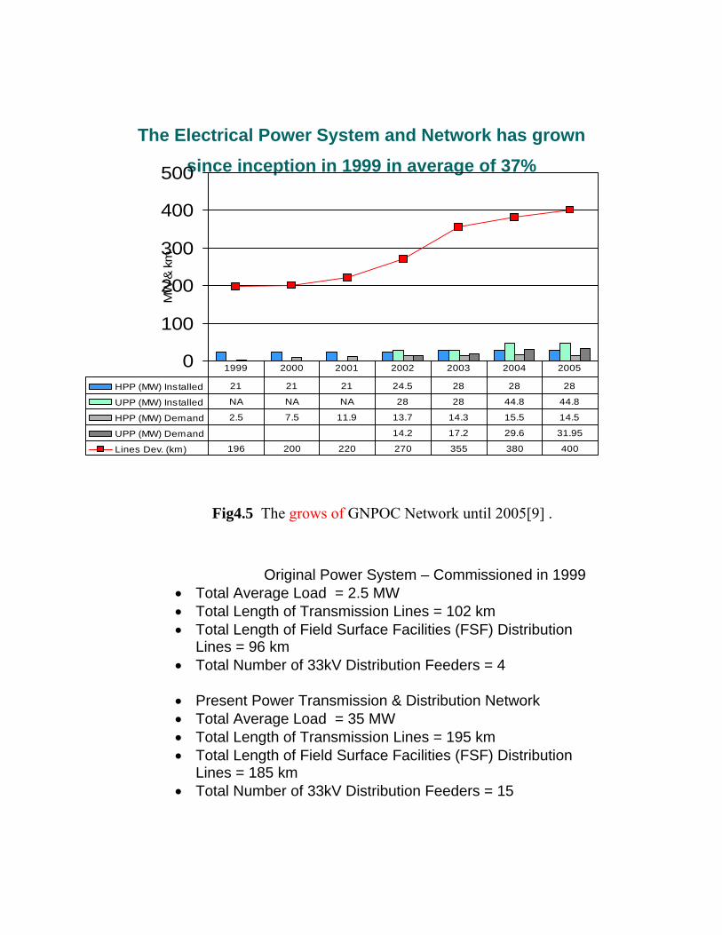
The Electrical Power System and Network has grown

since inception in 1999 in average of 37%

Fig4.5 The grows of GNPOC Network until 2005[9] .

0

100

200

300

400

500M

W &

km

HPP (MW) Installed 21 21 21 24.5 28 28 28

UPP (MW) Installed NA NA NA 28 28 44.8 44.8

HPP (MW) Demand 2.5 7.5 11.9 13.7 14.3 15.5 14.5

UPP (MW) Demand 14.2 17.2 29.6 31.95

Lines Dev. (km) 196 200 220 270 355 380 400

1999 2000 2001 2002 2003 2004 2005

Original Power System – Commissioned in 1999 • Total Average Load = 2.5 MW • Total Length of Transmission Lines = 102 km • Total Length of Field Surface Facilities (FSF) Distribution

Lines = 96 km • Total Number of 33kV Distribution Feeders = 4

• Present Power Transmission & Distribution Network • Total Average Load = 35 MW • Total Length of Transmission Lines = 195 km • Total Length of Field Surface Facilities (FSF) Distribution

Lines = 185 km • Total Number of 33kV Distribution Feeders = 15

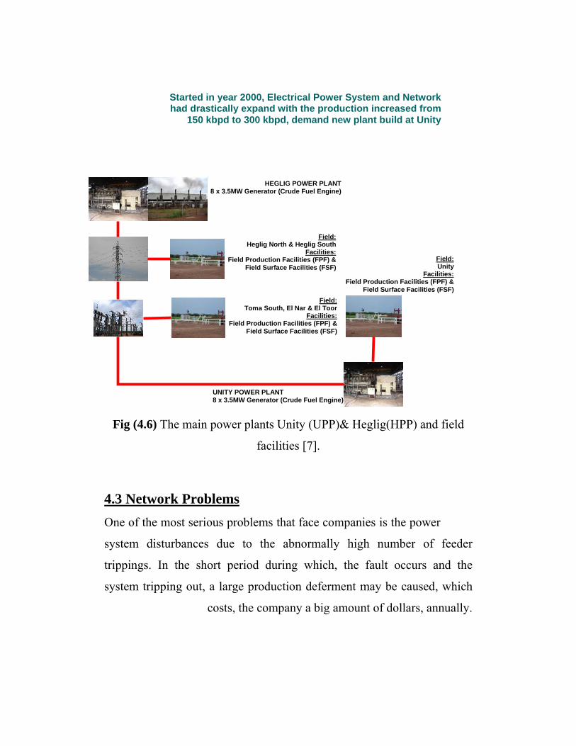
Fig (4.6) The main power plants Unity (UPP)& Heglig(HPP) and field

facilities [7].

4.3 Network Problems One of the most serious problems that face companies is the power

system disturbances due to the abnormally high number of feeder

trippings. In the short period during which, the fault occurs and the

system tripping out, a large production deferment may be caused, which

costs, the company a big amount of dollars, annually.

Started in year 2000, Electrical Power System and Network had drastically expand with the production increased from

150 kbpd to 300 kbpd, demand new plant build at Unity

HEGLIG POWER PLANT 8 x 3.5MW Generator (Crude Fuel Engine)

:Field Heglig North & Heglig South

:Facilities Field Production Facilities (FPF) &

Field Surface Facilities (FSF)

:Field Toma South, El Nar & El Toor

:Facilities Field Production Facilities (FPF) &

Field Surface Facilities (FSF)

:Field Unity

:Facilities Field Production Facilities (FPF) &

Field Surface Facilities (FSF)

UNITY POWER PLANT 8 x 3.5MW Generator (Crude Fuel Engine)

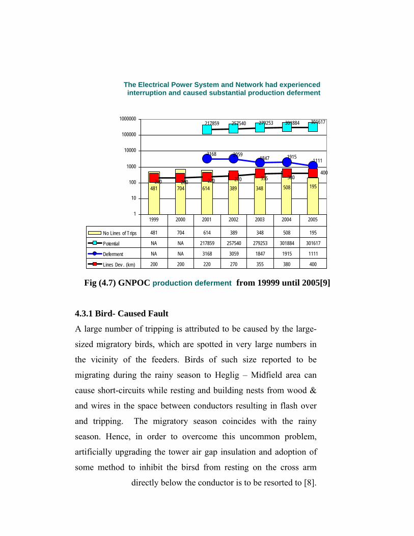
Fig (4.7) GNPOC production deferment from 19999 until 2005[9]

4.3.1 Bird- Caused Fault

A large number of tripping is attributed to be caused by the large-

sized migratory birds, which are spotted in very large numbers in

the vicinity of the feeders. Birds of such size reported to be

migrating during the rainy season to Heglig – Midfield area can

cause short-circuits while resting and building nests from wood &

and wires in the space between conductors resulting in flash over

and tripping. The migratory season coincides with the rainy

season. Hence, in order to overcome this uncommon problem,

artificially upgrading the tower air gap insulation and adoption of

some method to inhibit the birsd from resting on the cross arm

directly below the conductor is to be resorted to [8].

The Electrical Power System and Network had experienced interruption and caused substantial production deferment

195508348389614704481

400

301617301884279253257540217859

111119151847

30593168

380355270220200200

1

10

100

1000

10000

100000

1000000

No Lines of Trips 481 704 614 389 348 508 195

Potential NA NA 217859 257540 279253 301884 301617

Deferment NA NA 3168 3059 1847 1915 1111

Lines Dev . (km) 200 200 220 270 355 380 400

1999 2000 2001 2002 2003 2004 2005

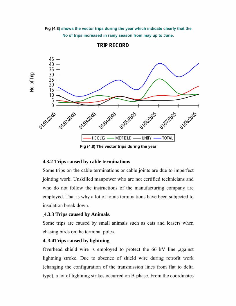
Fig (4.8) shows the vector trips during the year which indicate clearly that the No of trips increased in rainy season from may up to June.

Fig (4.8) The vector trips during the year

4.3.2 Trips caused by cable terminations

Some trips on the cable terminations or cable joints are due to imperfect

jointing work. Unskilled manpower who are not certified technicians and

who do not follow the instructions of the manufacturing company are

employed. That is why a lot of joints terminations have been subjected to

insulation break down.

4.3.3 Trips caused by Animals.

Some trips are caused by small animals such as cats and leasers when

chasing birds on the terminal poles.

4. 3.4Trips caused by lightning

Overhead shield wire is employed to protect the 66 kV line ,against

lightning stroke. Due to absence of shield wire during retrofit work

(changing the configuration of the transmission lines from flat to delta

type), a lot of lightning strikes occurred on B-phase. From the coordinates

TRIP RECORD

05

1015202530354045

01/01/

2005

01/02/

2005

01/03/

2005

01/04/

2005

01/05/

2005

01/06/

2005

01/07/

2005

01/08/

2005

No. o

f Trip

HEGLIG MIDFIELD UNITY TOTAL

of the locations of shield wire and the phase conductors on the tower, the

shielding angle offered by the overhead shield wire could be obtained for

the cases of the insulator string having 4 insulators in the string and for 5

insulators in the string. As per the standard design practice, shield angle

of more than 30 ° is considered to be inferior. Hence the 66 kV line could

be prone to lightning-caused over voltages and related tripping. This is

evident from the readings of the surge arrestor counters [8]. Hence a

substantial number of lightning-related insulation breakdowns could be

expected in on the top phase of the 66 kV line calling for additional

lightning protection for it.

4.3.5 Trips caused by Protection sensitivity

Settings of over-voltage and under-voltage relays of pumps (ESP) are

under international requirement (50%), but the majority are tuned to +-

5% so, they do not withstand any over or under voltage and therefore they

are too sensitive to the power tripping. The same thing is true for the

frequency relays .Moreover, protection grading time settings for the main

breaker at the power plants (40ms) and auto recloser on the overhead

lines (OHL) (70ms).

4.3.6 Trips caused by Harmonics

Harmonic levels of both voltage and current were recorded for some

important feeders at Heglig, Midfield, Unity and Bamboo. In all these

locations the dominating harmonic orders for voltage and current were

5th and 7th. The highest measured 5th harmonic component in the current

varied between 0.5% of fundamental and 19.4% of fundamental; and the

highest measured 5th harmonic voltage varied between 0.83%; of

fundamental and 2.9% of fundamental. The maximum Total Harmonic

Distortion ofthe current was 21.5 and the value for voltage was 3.5[8].

The presence of high content of harmonics in the voltage and

current (Distortion factor less than 20%) is known to make the relay

operation sluggish and not operate faster and / or lower pickup values

(refer IEEE Std. 519 – 1992, “IEEE Recommended practices and

requirements for harmonic control in electrical power systems). In

addition, the present day numerical relays, as employed by GNPOC, are

not expected to malfunction for the harmonic levels mentioned above.

4.3.7 Trips caused by H.V Fuses

Some High Voltage (H.V) fuses have different time current

characteristics. Consequently the main circuit breaker in the power plants

senses the fault before the fuses are blown out and hence a complete

power trip on the respective line occurs.

4.4- Trip Record

Based on the analysis, causes of the line trips can be categorized as

follows:

Fig (4.9, 10) shows common causes of line trips .

Trip analysis revealed that there are common causes of lines trip which can be categorized into various categories

Fig (4.9,10) Common causes of line trips

Fig (4.10) Common causes of lines trip

INS5%

CBL FLT11%

ABFI/ABI4%

ANML16%

Others16%

SA1%

Unknown32%

15%

15.7%

6.2%

1.7%

12.4%

5.1%

15.7% 15.7%

27.5%

0.0%

5.0%

10.0%

15.0%

20.0%

25.0%

30.0%

Ligh

tnin

g

Insu

lato

r

Surg

e Ar

rest

or

Cabl

e Fa

ult

ABFI

& A

BI

Anim

al

Othe

rs

Unkn

own

Analysis

• Lightning effect contribute 15%

of the total trip

• Cable fault count 11% of the trip

• Animal intervention contribute

16% of the trip causes

• Others records, 16% of trip

cause which were noted,

t ib t f t k

As advised by Experts from the University of Khartoum ,

CENTRAL POWER RESEARCH INSTITUTE- BANGALORE-INDIA

and PETRONAS in their studies ,most studies were assessment

processes to highlight the underlying causes in respect to design ,

construction & O&M .See following solutions :

Initiatives Implemented .44

A number of initiatives were carried out to resolve the issues

including retrofit and line enhancement. These may be summarized as

follows:

Year 2000: All the angle pole Jumpers replaced by HDPE Sleeves

Year 2001:Heglig Field Service Facility(FSF) Lines retrofitted

Year 2002: Unity Field Service Facility(FSF) Lines retrofitted

Year 2003: Midfield FSF Lines retrofitted

Year 2003: Pin Insulator jumpers replaced with XLPE (90% completed)

Year 2003: Section pole Jumpers replaced with HV heat shrinkable sleeves. (70% completed)

Year 2003: Insulation Enhancement (taping) on the road crossing cables. (30% completed)

8.7.6.

5. 4.3.2.1.No

UnknowUnknownOtherOthersANMLBirds

ABFI/ABI

Air Break Fused Isolator & Air

B k I l t

CBLCable FaultSASurge Arrestor

INSInsulatorLPSLightning

CodeCategory

Improvement Initiatives Implemented:

33 KV network sectionalized to reduce the impact on

production loss due to any tripping (production loss reduced by

75% by introducing 15 new breakers in the 33 KV network)

Main Heglig-Unity Transmission Line Upgraded from 33KV to

66KV to enhance the power transfer capability

Installed underground cable network, instead of O-H Lines, for

all the new fields to eliminate the bird faults

Changed of the design for the new Transmission Lines as well

as for FSF lines, to improve the conductor- tower air clearance

Modify HV terminal boxes of the well site ABB transformers &

redo the termination (on-going)

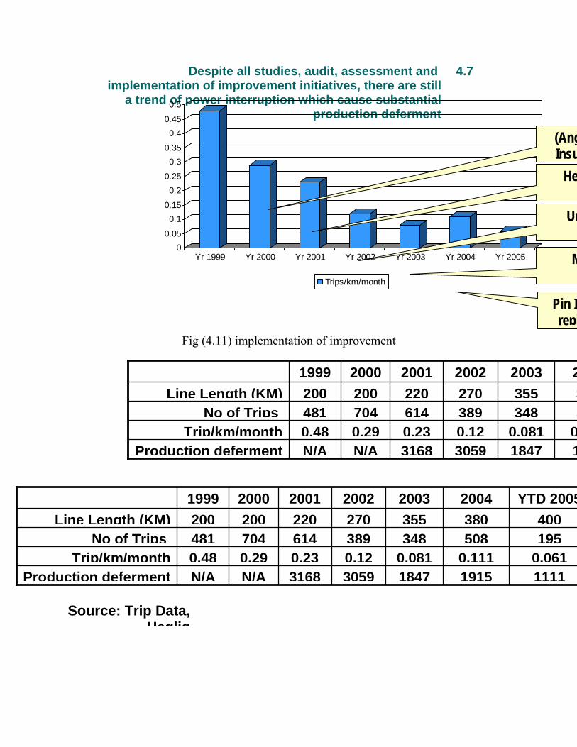
4.7 Despite all studies, audit, assessment and implementation of improvement initiatives, there are still

a trend of power interruption which cause substantial production deferment

Fig (4.11) implementation of improvement

PTER FIVE STABILITY ANAL

11110.061195400

YTD 2005

19150.111508380

2004 355270220200200Line Length (KM)348389614704481No of Trips

0.0810.120.230.290.48Trip/km/month184730593168N/AN/AProduction deferment

2003200220012000 1999

00.05

0.10.15

0.20.25

0.30.35

0.40.45

0.5

Yr 1999 Yr 2000 Yr 2001 Yr 2002 Yr 2003 Yr 2004 Yr 2005

Trips/km/month

(Ang Insu

He

Un

M

Pin Irepl

Source: Trip Data, Heglig

10532

355270220200200Line Length (KM)348389614704481No of Trips

0.0810.120.230.290.48Trip/km/month184730593168N/AN/AProduction deferment

20032002 200120001999

Heglig Grid Fault Analysis

5.1 Introduction Fault studies are carried out for the HEGLIG GRID, to verify the

nominal capacities of switchgear ,for the existing and planned systems,

and additionally for any protection system design, network equipment

design, and further it can be used for any network analysis.

HEGLIG GRID was analyzed for the following types of faults:

1-Balanced three phase fault.

2- Single line to ground fault.

3-Line to line fault.

4-Double line to ground fault.

One of the most common types of faults that affect Heglig grid is

the single line to ground fault which is caused by birds. It should be noted

that open circuit faults (series faults) were not included, because their

analysis is of little practical usel.

The study is presented with the consideration that all generators are

connected, thus the results obtained give the maximum short-circuit

currents. To compute the fault current, the bus voltages and line currents

during the fault, all shunt capacitances and loads are neglected and all the

prefault bus voltages are assumed to be unity.

The analysis was performed using the MATLAP PROGRAMM version 7

,which is described in chapter 3 .The basic data of Heglig Grid which are

necessary for carrying out fault analysis are shown in tables (5.1),( 5.2)

Gen.NO Ra X'd X0 Xn

1 o .20 0.06 0.05

10 o .15 0.04 0.05

11 o .25 0.08 0.00

Table(5.1) Transient Impedance in PU

The line and transformer data containing the series resistance and

reactance in per unit and one –half of the total capacitance in per unit

suseptance on a100-MVA base are tabulated in table 5.2.

Bus No Bus No R X 1/2 B Pu 1 2 0 .06 0.0 2 3 0.08 .3 .0004 2 5 .04 .15 .0002 2 6 .12 .45 .0005 3 4 .1 .4 .0005 3 6 .04 .4 .0005 4 6 .15 .60 .0008 4 9 .18 .7 .0009 4 10 0 .08 0.0 5 7 .05 .43 .0003 6 8 .06 .48 0.0 7 8 .06 .35 0.0004 7 11 0 .1 0.0 8 9 .052 .48 0.0

Table (5.2) Line and Transformer Data

5.2 Symmetrical Fault Simulation

Neglecting the shunt capacitors and the loads, zbuild(zdata)

function was used to obtain the bus impedance matrix for Heglig

Network which isshown in SLD appendix A. Assuming all the prefault

bus voltages are equal to 1.0 00 ∠ we use symfault function to compute the

fault currents for fault at bus 8. When using zbuild function, generator

reactance’s must be included in the impedance data with bus zero as the

reference bus the symfault program for Heglig Network to determine the

prefault conditions, solution of the network (Program $Result is given in

appendix E).

**********SYMFAULT PROGRAMS FOR HEGLIG *********

5.3 Unbalanced Fault Simulation

The lgfault' llfault, and dlgfault functions were used to compute

the fault current, bus voltages and line currents of HEGLIG GRID for the

following faults .

(a)A single-line-to-ground fault at bus 3 through fault impedance

0.1 fZ j per unit=

(b) A line-to-line fault at bus 3 through a fault impedance

0.1 fZ j per unit= .

(c) A Double-line-to-ground fault at bus 3 through fault impedance

0.1 fZ j per unit=

All shunt capacitances and loads are neglected and all prefault bus

voltages are assumed to be unity .The positive-sequence impedance

diagram is described by the variable zdata1 and the zero-sequence

impedance is described by the variable zdata0.The negative-sequence

data is assumed to be the same as the positive-sequence data .The

following commands were used. The lgfault' llfault, and dlgfault

program for Heglig Network to determine the prefault conditions,

solution of the network (Program $Result is given in appendix F).

****UNBALANCE FAULT PROGRAMS FOR HEGLIG*****

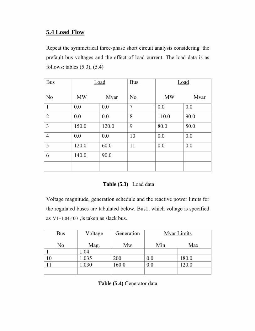
5.4 Load Flow

Repeat the symmetrical three-phase short circuit analysis considering the

prefault bus voltages and the effect of load current. The load data is as

follows: tables (5.3), (5.4)

Bus

No

Load

MW Mvar

Bus

No

Load

MW Mvar

1 0.0 0.0 7 0.0 0.0

2 0.0 0.0 8 110.0 90.0

3 150.0 120.0 9 80.0 50.0

4 0.0 0.0 10 0.0 0.0

5 120.0 60.0 11 0.0 0.0

6 140.0 90.0

Table (5.3) Load data

Voltage magnitude, generation schedule and the reactive power limits for

the regulated buses are tabulated below. Bus1, which voltage is specified

as V1=1.04 00 ∠ ,is taken as slack bus.

Bus

No

Voltage

Mag.

Generation

Mw

Mvar Limits

Min Max 1 1.04 10 1.035 200 0.0 180.0 11 1.030 160.0 0.0 120.0

Table (5.4) Generator data

Any of the power flow programs can be used to obtain the prefault

bus voltages and the load admittance .The Ifnewton program is used

which returns the prefault bus voltage array V and the bus load

admittance array yload. The required commands are as follows. The

Ifnewton program for Heglig Network to determine the prefault

conditions, solution of the network (Program $Result is given in appendix

(G).

Fault bus No. Fault type Current P.U Current

K.A K.V

Circuit Breaker capacity

K.A 8 3 – ph Sym fault 3.3319 17,498.56 11 31.5 5 ' ' 4.2519 7,434.81 33 31.5 3 ' ' 4.2476 3,720.09 66 31.5 1 ' ' 7.3203 12,800.1889 33 31.5 Unbalance fault 31.5 8 Single line – to -

ground 2.8290 14,857.41 11 31.5

5 ' ' 4.0803 7,134.764 33 31.5 3 ' ' 3.8032 3,330.88 66 31.5 1 ' ' 3.8032 10,890.03 33 31.5 8 Line – to – line 2.9060 1,5261.8 11 31.5 5 ' ' 3.7204 6,505.446 33 31.5 3 ' ' 3.7169 3,255.29 66 31.5 1 ' ' 6.3644 11,128.7 33 31.5 8 Double line – to –

ground 3.1527 16,557.34 11 31.5

5 ' ' 4.1971 7,338.99 33 31.5 3 ' ' 4.0902 3,582.24 66 31.5 1 ' ' 6.9142 12,090.87 33 31.5

Table (5.4) the result of fault currents

From the results obtained in above table (5.4) it is found that the

installed short circuit capacities of the circuit breakers (31.5K.A) are

reasonable compared to calculated values.

Conclusions & Recommendations 6.1 Conclusions

• Fault currents and voltages, have been obtained at each bus

.Therefore; fault level at each bus bar can easily be calculated.

Knowledge of the Fault level at each bus bar is very important for

the design ,sizing of the protective systems and sizing circuit

breakers

• The information gained from fault studies in this research, can be

used for proper relay settings, to verify the nominal capacities of

switchgear for the existing and planned systems, for network

design and for any network analysis.

• All types of fault currents in 11kv, 33kv and66 kV system are still

less than the rated capacities of the switchgears.

• The maximum value of fault current is the 3-ph symmetrical fault

type.

• This program is flexible and can be used in the future for any

analysis in Heglig grid. In case of modification in the system just

GNPOC simply has to enter the new data and clear the existing

data.

• This study will be useful where it is used in conjunction with other

studies covering the construction modification, designation and

coordination of the protective systems.

6.2 Recommendations 6.2.1 Relay Performance

• With the type of load on the 33 kV Well-feeders, transient inrush

currents due to switching of the pumps cannot be ruled out. Digital

/ numerical relays can be best exploited to ascertain the occurrence

of line tripping due to inrush current magnitude and/or duration. If

it is found to be happening, it is probable that the sensitivity of

relays could be high, causing spurious tripping. The relay

manufacturer shall be approached to reduce the sensitivity of

relays without sacrificing the protection requirements.

• In the absence of the record for checking the settings and

performance of relays after their installation, it is strongly

recommended that a competent agency could be approached to

check the relay performance in the field.

• It is also recommended that, when a change in the topology of the

distribution network changes, a check on the requirements of relay

settings and fuse characteristics be made by carrying out relay and

fuse coordination study by a competent agency.

6.2.2 Further Recommendation • Significant changes in frequency are quite enough to initiate the

protection schemes of submarine oil pump to trip out the pumps.

The suggestion is to increase the margin of frequency that initiates

the protection schemes. Inertia constant of the machines should be

taken in account.

• Fault currents (line to ground and double line to ground) must be

limited to reasonable values .For Limitations of short-circuit

currents it is recommended to use current-limiting reactors.

Moreover, ungrounded system shall be studied to assess the system

.The research focus is on the line-to earth fault, because it is the

common fault in Heglig (90% of the total faults occurring in the

Heglig gird is earth fault).

• For the11kv, 33kv and66 kV levels recommended circuit breakers

will have short- current values not less than 31.5 KA for the

present and future design specification.

• The program used in this research can be used for other types of

protection schemes with more delay times to avoid transient

disturbances which are cleared automatically (duration

proportional to currents) in order to decrease the number of trips,

because the faults are momentary and are automatically cleared.

References

1. William D.Stevenson, Element Of Power System Analysis,

Fourth Edition. Singapore.Mc Graw-Hill Book Co.1982.

2. R. Bergin-Vijay Vittal, Power System Analysis, Prentice Hall,

Upper Saddle River, New Jersey 2000.

3. Hadi Saadat, Power System Analysis, Singapore.Mc Graw-Hill

Book Co.1999.

4. Prabha Kundur, Power System Stability and Control, McGraw-

Hill, Inc. New York 1994.

5. R. Sunil S. Rao, Switchgear Protection and Power Systems,

Eleven Edition.Khanna Publishers.Delhi – 110006.

6. Dr. S.L. Uppal, Electrical Power, Eleven Edition.Khanna

Publishers.Delhi

7. Petroleum National Berhead (PETRONAS), Assessment of

GNPOC Electrical Power System. Heglig 4th Oct 2005

8. Bangalore India ,Central Power Research Institute, Heglig

2005 9. Trip Data, Heglig Power system

10. e-mail: saadat@msoe.edu

11. Matlap source version7.