fatigue reliability of gas turbine engine structures · pdf filefatigue reliability of gas...
TRANSCRIPT
NASA/CRD97-206215
Fatigue Reliability of Gas Turbine
Engine Structures
Thomas A. Cruse, Sankaran Mahadevan, and Robert G. Tryon
Vanderbilt University, Nashville, Tennessee
Prepared under Grant NGT-51053
National Aeronautics and
Space Administration
Lewis Research Center
October 1997
https://ntrs.nasa.gov/search.jsp?R=19970041395 2018-05-17T18:21:53+00:00Z

NASA Center for Aerospace Information
800 Elkridge Landing Road
Linthicum Heights, MD 21090-2934Price Code: A04
Available from
National Technical Information Service
5287 Port Royal Road
Springfield, VA 22100Price Code: A04
FATIGUE RELIABILITY OF GAS TURBINE ENGINE STRUCTURES
Thomas A. Cruse, Sankaran Mahadevan, and Robert G. Tryon
Vanderbilt University, Nashville, Tennessee
Abstract
The results of an investigation are described for fatigue reliability in engine structures. The
description consists of two parts. Part I is for method development. Part II is a specific case
study. In Part I, the essential concepts and practical approaches to damage tolerance design in
the gas turbine industry are summarized. These have evolved over the years in response to flight
safety certification requirements. The effect of non-destructive evaluation (NDE) methods onthese methods is also reviewed. Assessment methods based on probabilistic fracture mechanics,
with regard to both crack initiation and crack growth, are outlined. Limit state modeling
techniques from structural reliability theory are shown to be appropriate for application to this
problem, for both individual failure mode and system-level assessment. In Part H, the results of a
case study for the high pressure turbine of a turboprop engine are described. The response
surface approach is used to construct a fatigue performance function. This performance function
is used with the first order reliability method (FORM) to determine the probability of failure and
the sensitivity of the fatigue life to the engine parameters for the first stage disk rim of the two
stage turbine. A hybrid combination of regression and Monte Carlo simulation is to use
incorporate time dependent random variables. System reliability is used to determine the system
probability of failure, and the sensitivity of the system fatigue life to the engine parameters of the
high pressure turbine. The variation in the primary hot gas and secondary cooling air, the
uncertainty of the complex mission loading, and the scatter in the material data are considered.
Part I - METHODOLOGIES
Summary
Part I is a review of the developmentof reliability assessmentmethodologiesfor gasturbineenginestructures.Theessentialconceptsandpracticalapproachesto damagetolerancedesigninthegasturbineindustryaresummarized.Thesehaveevolvedovertheyearsin responseto flightsafetycertification requirements.The effect of non-destructiveevaluation(NDE) methodsonthesemethodsis alsoreviewed. Assessmentmethodsbasedonprobabilisticfracturemechanics,with regard to both crack initiation and crack growth, are outlined. Limit statemodelingtechniquesfrom structuralreliability theoryareshownto be appropriatefor applicationto thisproblem,for both individual failure modeand system-levelassessment.Theseareobservedtoprovide useful sensitivity information on the influence of various engine parameterson thereliability.
Introduction
The reliability of a gas turbine engine structure is affected by the uncertainties in the operating environment
(speed, temperature etc.) as well as in the structural properties (material properties, geometries, boundary
conditions etc.). Traditional design methods generally account for these uncertainties using experience-based
design safety margins. However, the statistical nature of fatigue and crack growth properties have long been
recognized and given increasingly appropriate treatment. For example, a common commercial certification
requirement is that the probability of crack initiation be less than 1/1000, recognizing the statistical basis
of this problem.
Several methodologies have been developed during the past several decades to address the problem of
fatigue and fracture reliability of gas turbine engine structures. These include crack initiation and crack
growth models, non-destructive evaluation, probabilistic risk assessment etc. Recent years have seen the
development of limit state modeling approaches to estimating component and system structural reliability,
including advances in response surface, ettieient simulation, and analytical approximation techniques. This
paper summari_es the development of the various methods for fatigue reliability assessment, and the advances
made by the gas turbine engine industry in applying these concepts. The companion paper (Part II) [43]
presents a case study in which the limit state modeling methodology is applied for individual crack as well
as system-level assessment.
1 Damage Tolerant Design in the Aeropropulsion Industry
For the most part, engine design today is driven by safe life design philosophy -- maximize the number of
flight cycles before cracking can be expected. This has been largely successful over the years, especially in
the commercial engine market, due to a very heavy emphasis placed on high performance materials, material
quality control, and processing control. The lead organization for much of this was Pratt & Whitney, as they
had 90% of the commercial market share in the 1960's and 1970's, when much of the production standards
on the part of suppliers was established.
The FAA life-certifies critical rotating structures in engines, such as disks, shafts, spacers, and hubs.
Some work is ongoing for life certifying static engine structures such as diffuser cases which see the same
stress levels as many rotating parts and failure of which is every bit as critical. Two engine manufacturers
certify the rotating parts on a minimum life basis, meaning that at the mandatory retirement life of the
parts, a statistically very small sample of the parts can be expected to have initiated a crack. The U.S.
Air Force refers to this safe life as the "economic life" of the part. Exposure to more flight cycles than this
limit results in a rapidly increasing number of cracked parts. The design basis of these two life methods
is different as Pratt & Whitney uses an empirical crack initiation model and Rolls Royce uses a fracture
mechanics model for initiation.
Around 1980, the U.S. Air Force Systems Command began to develop the engine structural integrity
program (ENSIP), patterned in appropriate ways after the successful ASIP standard. Much of the work in
development of the ENSIP handbook [3] was validated through application to the Pratt & Whitney F-100
engine. Non-destructive evaluation (NDE) standards were reviewed, improved, and extended, as well as were
the processes and process controls, as a result of that effort. All components received a detailed fracture
mechanics analysis for NDE-sized flaws to determine the depot inspection intervals.
As a result of the durability review of the F-100 engine, it was found that the operating stress level and
material crack growth rates in engine structures did not readily support damage tolerance. That is, the
resulting depot level inspections would be required at uneconomically short intervals, based on the existing
NDE capabilities. As a result, the San Antonio Air Logistics Center implemented cryogenic proof spin testing
of the F-100 first stage fan, as well as elaborate, automated eddy current component inspection methods in
order to establish highly sensitive NDE capabilities [26].
Very high strength turbine wheel designs in the 1970's started using powder metallurgy (PM) nickel base
superalloys, such as the Pratt & Whitney IN100 and the General Electric Rend 95 alloys. Due to prior
commercial experience with PM disk design, Pratt & Whitney established very stringent powder handling
andprocessingstandards. Considerable emphasis was placed on characterizing the intrinsic defects in these
materials, for example [19], in order to define more durable standards as well as to establish a fracture
mechanics design basis for the materials. Again, this effort followed that in the commercial arena at Pratt
& Whitney, but that commercial work was proprietary and still has not been adequately published.
The U.S. Air Force initiated an effort to increase the damage tolerance of powder metallurgy, nickel base
superalloys. It was found that a coarsening of the grain structure resulged in slower crack growth rates.
The trade-off was that the crack initiation life of the material decreased, thereby decreasing the economic
life limits of the parts. Damage tolerance was selected as the more important design concern in the final
material process selection.
Engine materials have high intrinsic strength and resulting fatigue capacity. This quality has always come
with a price. For example, a single nickel superalloy disk may cost well in excess of $50K. The U.S. Air Force
observed that there was much wasted money in the old method of retiring disks at an economic life limit,
because so few might be expected to be cracked. As a result, the "retirement for cause" (RFC) philosophy
of disk lifing was investigated [44], [22]. The RFC approach was to combine the inspection processes being
developed by the damage tolerance requirements with an indefinite life limit of engine parts, such that a
part stayed in service until it was found to be cracked; when cracked, the part was to be removed from
service. Significant probabilistic fracture mechanics issues were uncovered in the RFC approach owing to
the exposure and liability associated with missed cracks [44].
During this time period, the commercial engine fleets were setting the pace in terms of applied fracture
mechanics of engine parts. Air Force and Navy engines were too few and acquiring cycles at too slow a rate
to challenge the life envelope the way the commercial engines were. For example, significant numbers of mid-
size commercial turbofan engines were first designed in the late 1950's and are still being sold (in updated
versions, of course) today. There are thousands of such engines, each of which has a high stressed titanium
fan disk, a high stressed nickel turbine disk, and multiple high stressed steel high pressure compressor
(HPC) disks. The certified life limits on the various designs range from 15,000 flights to 20,000 flights. Some
operators might accumulate in excess of 2,000 fatigue cycles a year.
Some design successes were clearly established by the commercial fleets. The titanium fan disks at Pratt
& Whitney were retired in such numbers by the early 1980's that one had very high statistical confidence
in the minimum fatigue life of the material. Equally high reliability was demonstrated for a number of
turbine disk designs as well. However, there were also some design problems in the late 1970's and 1980's.
It was found, for example, that the stresses in engine disks had not been adequately calculated in the early
design periods, prior to the use of the finite element method. As a result, several engine models had disks
which would not reach their initial design life. Damage tolerance assessments were made using probabilistic
fracture mechanics to determine what inspection intervals could be imposed without undue risk to the total
fleet operations of the affected engines.
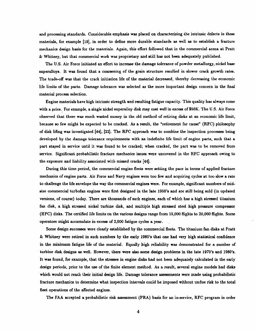
The FAA accepted a probabilistic risk assessment (PRA) basis for an in-service, RFC program in order
4
Part
Histogram
Cumulative
% PartsCracked
to 1/32"
1.1
Cycles
"INITIATION" -}-
Scatter
_'_m Crack
Size
Inspect.)(!Disk Limits
Establishes
Exposure_ J
•No Inspection
"L__ Inspection
Program;"Drawdown"
Limits
Propagation• Scatter
I
RELIABILITY
OFCRACK
DETECTION
"Monte Cede" Simulations
RISKASSESSMENT
let inspectionlimit
o Roinspectionlimit, Inspectionsensitivity
o inspectionreliability
t
Cycles Cycles, TJ( +
No
Inspect,
Figure 1: Probabilistic Risk Assessment Flow Diagram for Disk Cracking
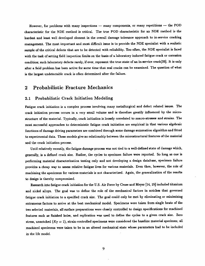
to minimize the number of aircraft engines that had to be removed from service due to field cracking. The
program was so successful that the FAA adopted the probabilistic risk assessment as the basis for all engine
disk in-service cracking problems. The elements of the PRA shown in Figure 1 include probabilistic models
for crack initiation, crack propagation, and NDE probability of detection (POD). The total fleet risk is
obtained by summing the individual element risks over the entire fleet of engine disks using the known,
current and future cyclic histogram. The inspection intervals are then adjusted in such a way to achieve the
desired level of risk of disk failure for the total fleet.
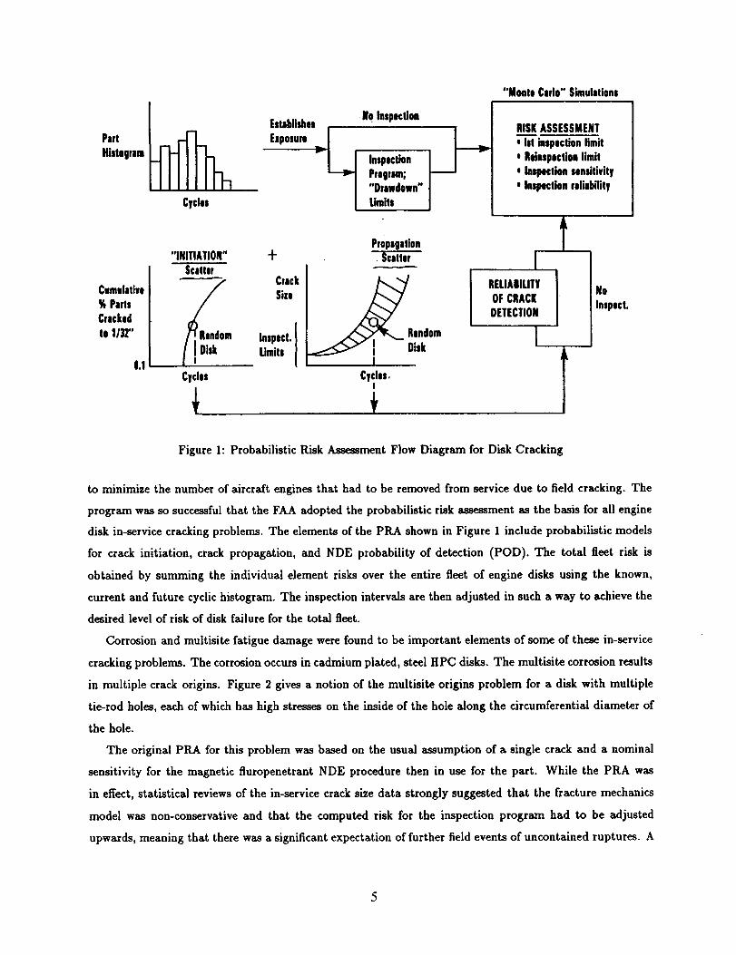
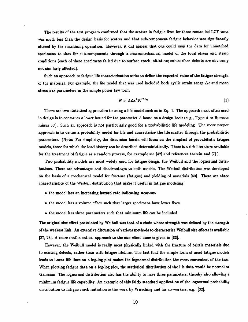
Corrosion and multisite fatigue damage were found to be important elements of some of these in-service
cracking problems. The corrosion occurs in cadmium plated, steel HPC disks. The multisite corrosion results
in multiple crack origins. Figure 2 gives a notion of the multisite origins problem for a disk with multiple
tie-rod holes, each of which has high stresses on the inside of the hole along the circumferential diameter of
the hole.
The original PRA for this problem was based on the usual assumption of a single crack and a nominal
sensitivity for the magnetic fluropenetrant NDE procedure then in use for the part. While the PRA was
in effect, statistical reviews of the in-service crack size data strongly suggested that the fracture mechanics
model was non-conservative and that the computed risk for the inspection program had to be adjusted
upwards, meaning that there was a significant expectation of further field events of uncontained ruptures. A
HPC Disk
ole Sec±ion (typ)
______Tie rod hole (typ)
Crack sites (±yp)
Figure 2: Typical HPC Disk with Multiple Corrosion-induced Fatigue Origins
review of the failed hardware from several incidents revealed that the multisite crack initiation process could
give rise to reduced fracture mechanics lives.
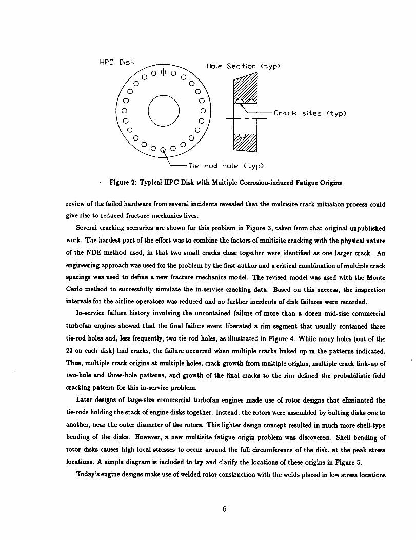
Several cracking scenarios are shown for this problem in Figure 3, taken from that original unpublished
work. The hardest part of the effort was to combine the factors of multisite cracking with the physical nature
of the NDE method used, in that two small cracks close together were identified as one larger crack. An
engineering approach was used for the problem by the first author and a critical combination of multiple crack
spacings was used to define a new fracture mechanics model. The revised model was used with the Monte
Carlo method to successfully simulate the in-service cracking data. Based on this success, the inspection
intervals for the airline operators was reduced and no further incidents of disk failures were recorded.
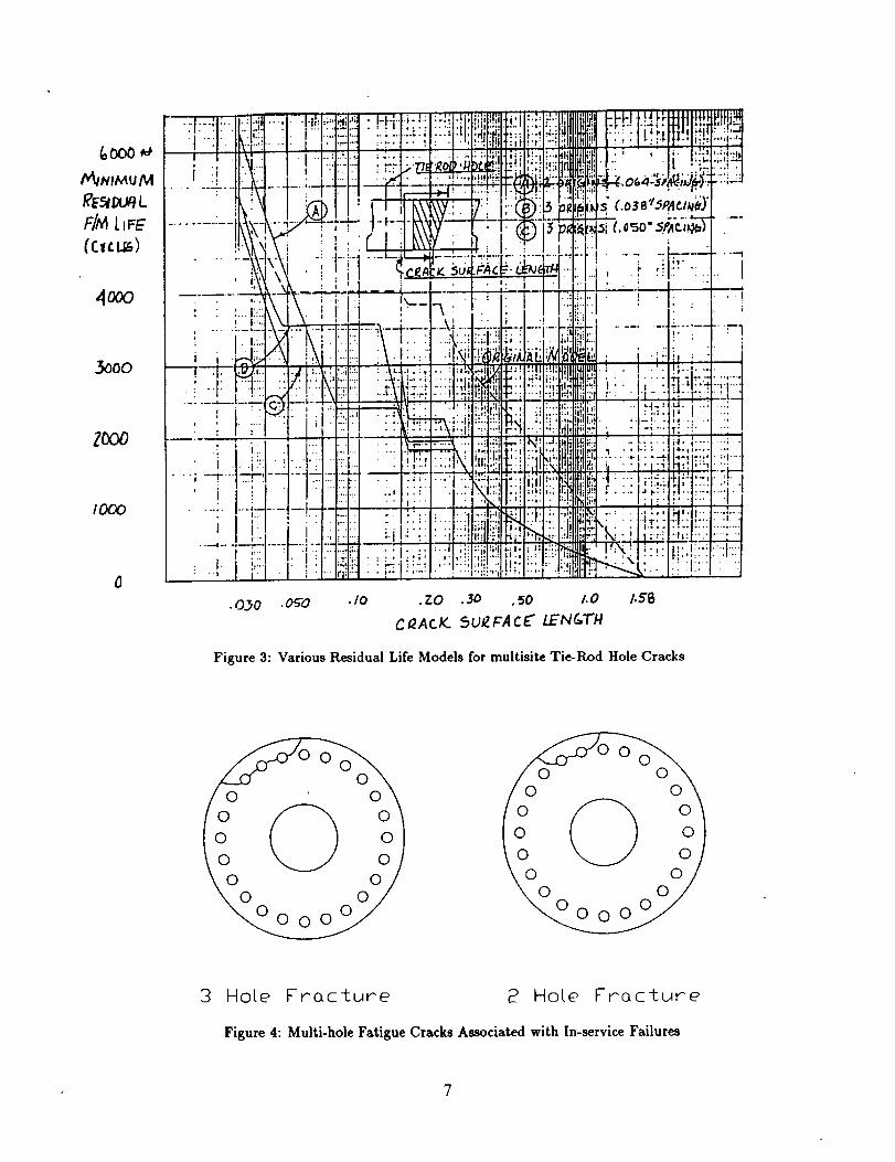
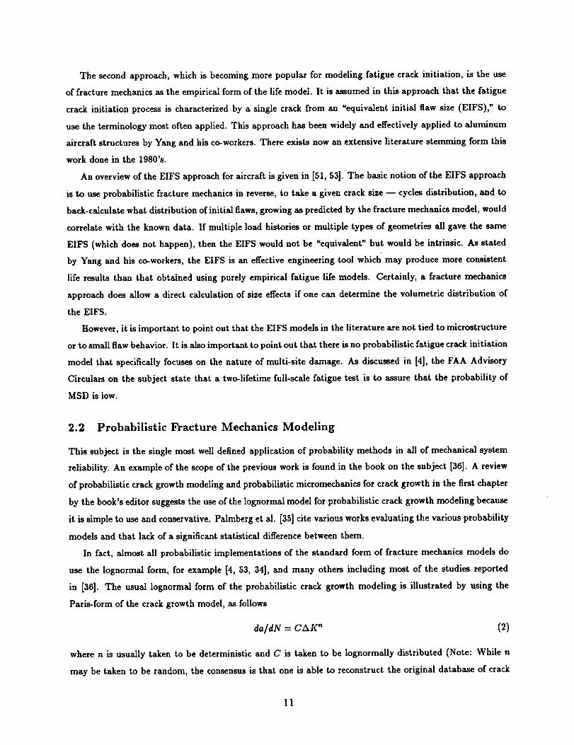
In-service failure history involving the uncontained failure of more than a dozen mid-size commercial
turbofan engines showed that the final failure event liberated a rim segment that usually contained three
tie-rod holes and, less frequently, two tie-rod holes, as illustrated in Figure 4. While many holes (out of the
23 on each disk) had cracks, the failure occurred when multiple cracks linked up in the patterns indicated.
Thus, multiple crack origins at multiple holes, crack growth from multiple origins, multiple crack link-up of
two-hole and three-hole patterns, and growth of the final cracks to the rim defined the probabilistic field
cracking pattern for this in-service problem.
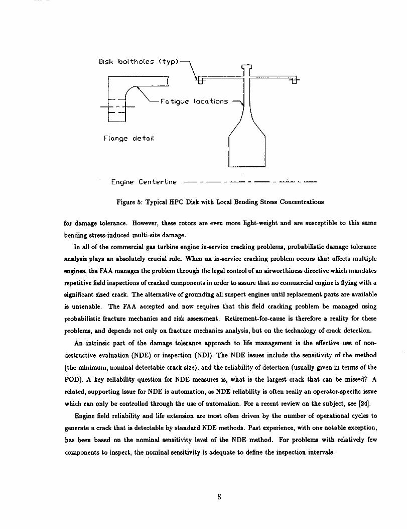
Later designs of large-size commercial turbofan engines made use of rotor designs that eliminated the
tie-rods holding the stack of engine disks together. Instead, the rotors were assembled by bolting disks one to
another, near the outer diameter of the rotors. This lighter design concept resulted in much more shell-type
bending of the disks. However, a new multisite fatigue origin problem was discovered. Shell bending of
rotor disks causes high local stresses to occur around the full circumference of the disk, at the peak stress
locations. A simple diagram is included to try and clarify the locations of these origins in Figure 5.
Today's engine designs make use of welded rotor construction with the welds placed in low stress locations
_ 000
tv mMvM
F/ 4 L
4ooo
3ooo
Zooo
I000
0
•0.._0 •Og'O •I0 .ZO .30 .50 1.0 I.E6C_ACK.. 5u£FACC I.EN&TH
Figure 3: Various Residual Life Models for multisite Tie-Rod Hole Cracks
3 Hole Frac±ure 2 HoLe Frc_cture
Figure 4: Multi-hole Fatigue Cracks Associated with In-service Failures
7
Engine Cen±er(ine
Figure 5: Typical HPC Disk with Local Bending Stress Concentrations
for damage tolerance. However, these rotors are even more light-weight and are susceptible to this same
bending stress-induced multi-site damage.
In all of the commercial gas turbine engine in-service cracking problems, probabilistic damage tolerance
analysis plays an absolutely crucial role. When an in-service cracking problem occurs that affects multiple
engines, the FAA manages the problem through the legal control of an airworthiness directive which mandates
repetitive field inspections of cracked components in order to assure that no commercial engine is flying with a
significant sized crack. The alternative of grounding all suspect engines until replacement parts are available
is untenable. The FAA accepted and now requires that this field cracking problem be managed using
probabilistic fracture mechanics and risk assessment. Retirement-for-cause is therefore a reality for these
problems, and depends not only on fracture mechanics analysis, but on the technology of crack detection.
An intrinsic part of the damage tolerance approach to life management is the effective use of non-
destructive evaluation (NDE) or inspection (NDI). The NDE issues include the sensitivity of the method
(the minimum, nominal detectable crack size), and the reliability of detection (usually given in terms of the
POD). A key reliability question for NDE measures is, what is the largest crack that can be missed? A
related, supporting issue for NDE is automation, as NDE reliability is often really an operator-specific issue
which can only be controlled through the use of automation. For a recent review on the subject, see [24].
Engine field reliability and life extension are most often driven by the number of operational cycles to
generate a crack that is detectable by standard NDE methods. Past experience, with one notable exception,
has been based on the nominal sensitivity level of the NDE method. For problems with relatively few
components to inspect, the nominal sensitivity is adequate to define the inspection intervals.
However,for problemswith many inspections m many components, or many repetitions -- the POD
characteristic for the NDE method is critical. The true POD characteristic for an NDE method is the
hardest and least well developed element in the overall damage tolerance approach to in-service cracking
management. The most important and most difficult issue is to provide the NDE specialist with a realistic
sample of the critical defects that are to be detected with reliability. Too often, the NDE specialist is faced
with the task of setting field inspection limits on the basis of a laboratory induced fatigue crack or corrosion
conditionl such laboratory defects rarely, if ever, represent the true state of an in-service crack[35]. It is only
after a field problem has been active for some time that real cracks can be examined. The question of what
is the largest undetectable crack is often determined after the failure.
2 Probabilistic Fracture Mechanics
2.1 Probabilistic Crack Initiation Modeling
Fatigue crack initiation is a complex process involving many metallurgical and defect related issues. The
crack initiation process occurs in a very small volume and is therefore greatly influenced by the micro-
structure of the material. Typically, crack initiation is loosely correlated to macro-stresses and strains. The
most successful approaches to deterministic fatigue crack initiation are empirical in that various algebraic
functions of damage driving parameters are combined through some damage summation algorithm and fitted
to experimental data. These models give no relationship between the microstructural features of the material
and the crack initiation process.
Until relatively recently, the fatigue damage process was not tied to a well-defined state of damage which,
generally, is a defined crack size. Rather, the cycles to specimen failure were reported. So long as one is
performing material characterization testing only and not developing a design database, specimen failure
provides a cheap way to assess relative fatigue lives for various materials. Even then, however, the role of
machining the specimens for various materials is not characterized. Again, the generalization of the results
to design is thereby compromised.
Research into fatigue crack initiation for the U.S. Air Force by Cruse and Meyer [14, 15] included titanium
and nickel alloys. The goal was to define the role of the mechanical factors in notches that governed
fatigue crack initiation to a specified crack size. The goal could only be met by eliminating or minimizing
extraneous factors to arrive at the best mechanical model. Specimens were taken from single heats of the
two selected materials, all surface preparations were closely controlled to design specifications for machined
features such as finished holes, and replication was used to define the cycles to a given crack size. Zero
stress, unnotched (KT = 1), strain-controlled specimens were considered the baseline material specimen; all
machined specimens were taken to be in an altered mechanical state whose parameters had to be included
in the life model.
The results of the test program confirmed that the scatter in fatigue lives for these controlled LCF tests
was much less than the design basis for scatter and that sub-component fatigue behavior was significantly
altered by the machining operation. However, it did appear that one could map the data for unnotched
specimens to that for sub-components through a macromechanical model of the local stress and strain
conditions (each of these specimens failed due to surface crack initiation; sub-surface defects are obviously
not similarly affected).
Such an approach to fatigue life characterization seeks to define the expected value of the fatigue strength
of the material. For example, the life model that was used included both cyclic strain range A¢ and mean
stress _rM parameters in the simple power law form
N = AAc_10 c°M (1)
There are two statistical approaches to using a life model such as in Eq. 1. The approach most often used
in design is to construct a lower bound for the parameter A based on a design basis (e. g., Type A or B; mean
minus 3_r). Such an approach is not particularly good for a probabilistic life modeling. The more proper
approach is to define a probability model for life and characterize the life scatter through the probabilistic
parameters. (Note: For simplicity, the discussion herein will focus on the simplest of probabilistic fatigue
models, those for which the load history can be described deterministically. There is a rich literature available
for the treatment of fatigue as a random process, for example see [42] and references therein and [7].)
Two probability models are most widely used for fatigue design, the Weibull and the lognormal distri-
butions. There are advantages and disadvantages to both models. The Weibull distribution was developed
on the basis of a mechanical model for fracture (fatigue) and yielding of materials [50]. There are three
characteristics of the Weibull distribution that make it useful in fatigue modeling:
• the model has an increasing hazard rate indicating wear-out
• the model has a volume effect such that larger specimens have lower lives
• the model has three parameters such that minimum life can be included
The original size effect postulated by Weibull was that of a chain whose strength was defined by the strength
of the weakest link. An extensive discussion of various methods to characterize Weibull size effects is available
[27, 28]. A more mathematical approach to the size effect issue is given in [33].
However, the Weibull model is really most physically linked with the fracture of brittle materials due
to existing defects, rather than with fatigue lifetime. The fact that the simple form of most fatigue models
leads to linear life lines on a log-log plot makes the lognormal distribution the most convenient of the two.
When plotting fatigue data on a log-log plot, the statistical distribution of the life data would be normal or
Ganssian. The lognormal distribution also has the ability to have three parameters, thereby also allowing a
minimum fatigue life capability. An example of this fairly standard application of the lognormal probability
distribution to fatigue crack initiation is the work by Wirsching and his co-workers, e.g., [32].
10
The second approach, which is becoming more popular for modeling fatigue crack initiation, is the use
of fracture mechanics as the empirical form of the life model. It is assumed in this approach that the fatigue
crack initiation process is characterized by a single crack from an "equivalent initial flaw size (EIFS)," to
use the terminology most often applied. This approach has been widely and effectively applied to aluminum
aircraft structures by Yang and his co-workers. There exists now an extensive literature stemming form this
work done in the 1980's.
An overview of the EIFS approach for aircraft is given in [51, 53]. The basic notion of the EIFS approach
is to use probabilistic fracture mechanics in reverse, to take a given crack size -- cycles distribution, and to
back-calculate what distribution of initial flaws, growing as predicted by the fracture mechanics model, would
correlate with the known data. If multiple load histories or multiple types of geometries all gave the same
EIFS (which does not happen), then the EIFS would not be "equivalent" but would be intrinsic. As stated
by Yang and his co-workers, the EIFS is an effective engineering tool which may produce more consistent
life results than that obtained using purely empirical fatigue life models. Certainly, a fracture mechanics
approach does allow a direct calculation of size effects if one can determine the volumetric distribution of
the EIFS.
However, it is important to point out that the EIFS models in the literature are not tied to microstructure
or to small flaw behavior. It is also important to point out that there is no probabilistic fatigue crack initiation
model that specifically focuses on the nature of multi-site damage. As discussed in [4], the FAA Advisory
Circulars on the subject state that a two-lifetime full-scale fatigue test is to assure that the probability of
MSD is low.
2.2 Probabilistic Fracture Mechanics Modeling
This subject is the single most well defined application of probability methods in all of mechanical system
reliability. An example of the scope of the previous work is found in the book on the subject [36]. A review
of probabilistic crack growth modeling and probabilistic micromechanics for crack growth in the first chapter
by the book's editor suggests the use of the lognormal model for probabilistic crack growth modeling because
it is simple to use and conservative. Palmberg et al. [35] cite various works evaluating the various probability
models and that lack of a significant statistical difference between them.
In fact, almost all probabilistic implementations of the standard form of fracture mechanics models do
use the lognormal form, for example [4, 53, 34], and many others including most of the studies reported
in [36]. The usual lognormal form of the probabilistic crack growth modeling is illustrated by using the
Paris-form of the crack growth model, as follows
da/dN -- CAK n (2)
where n is usually taken to be deterministic and C is taken to be lognormally distributed (Note: While n
may be taken to be random, the consensus is that one is able to reconstruct the original database of crack
11
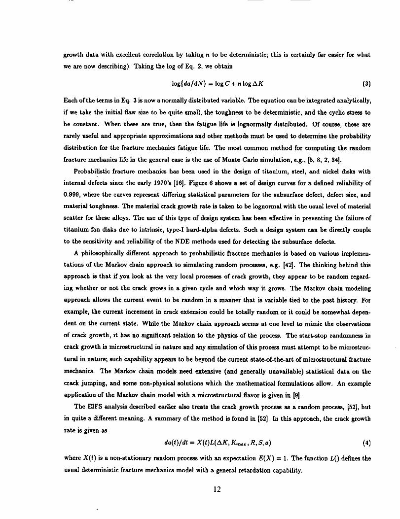
growth data with excellent correlation by taking n to be deterministic; this is certainly far easier for what
we are now describing). Taking the log of Eq. 2, we obtain
log{da/dN} - log C + n log AK (3)
Each of the terms in Eq. 3 is now a normally distributed variable. The equation can be integrated analytically,
if we take the initial flaw size to be quite small, the toughness to be deterministic, and the cyclic stress to
be constant. When these are true, then the fatigue life is lognormally distributed. Of course, these are
rarely useful and appropriate approximations and other methods must be used to determine the probability
distribution for the fracture mechanics fatigue life. The most common method for computing the random
fracture mechanics life in the general case is the use of Monte Carlo simulation, e.g., [5, 8, 2, 34].
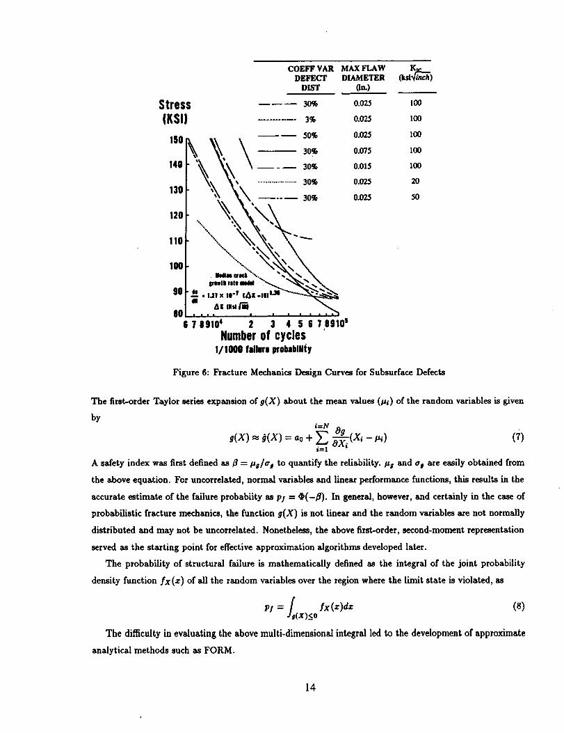
Probabilistic fracture mechanics has been used in the design of titanium, steel, and nickel disks with
internal defects since the early 1970's [16]. Figure 6 shows a set of design curves for a defined reliability of
0.999, where the curves represent differing statistical parameters for the subsurface defect, defect size, and
material toughness. The material crack growth rate is taken to be lognormal with the usual level of material
scatter for these alloys. The use of this type of design system has been effective in preventing the failure of
titanium fan disks due to intrinsic, type-I hard-alpha defects. Such a design system can be directly couple
to the sensitivity and reliability of the NDE methods used for detecting the subsurface defects.
A philosophically different approach to probabilistic fracture mechanics is based on various implemen-
tations of the Markov chain approach to simulating random processes, e.g. [42]. The thinking behind this
approach is that if you look at the very local processes of crack growth, they appear to be random regard-
ing whether or not the crack grows in a given cycle and which way it grows. The Markov chain modeling
approach allows the current event to be random in a manner that is variable tied to the past history. For
example, the current increment in crack extension could be totally random or it could he somewhat depen-
dent on the current state. While the Markov chain approach seems at one level to mimic the observations
of crack growth, it has no significant relation to the physics of the process. The start-stop randomness in
crack growth is microstructural in nature and any simulation of this process must attempt to be microstruc-
turai in nature; such capability appears to be beyond the current state-of-the-art of microstructural fracture
mechanics. The Markov chain models need extensive (and generally unavailable) statistical data on the
crack jumping, and some non-physical solutions which the mathematical formulations allow. An example
application of the Markov chain model with a microstructural flavor is given in [9].
The EIFS analysis described earlier also treats the crack growth process as a random process, [52], but
in quite a different meaning. A summary of the method is found in [52]. In this approach, the crack growth
rate is given as
da(t)/dt = X(OL(ZXK , K,,,,,, R, S, a) (4)
where X(t) is a non-stationary random process with an expectation E(X) = 1. The function L 0 defines the
usual deterministic fracture mechanics model with a general retardation capability.
12
Yang et al. take X(t) to be a lognormal random process. If we take Z(t) = logX(t), then the autocor-
relation function for the random process in log-space is given as
R,:(r) = E[Z(t)Z(t + r)] (5)
Since the autocorrelation function in gq. 5 is a function of r only, the process is stationary. The Fourier
transform of the autocorrelation function in Eq. 5, denoted _z,(w), is the power spectral density of the
lognormal random process. When the random process is completely correlated at any two time instants,
then the random process X(t) becomes a random variable X. The random crack growth process then
becomes the lognormal random variable crack growth model, given by
da(t)/dt = XQa (t)ao
a(t) =[1 - Xeta_)]ll"
(e)
where e = b-1. In [53], the authors state that the fully correlated model in Eq. 7 gives the greatest dispersion
of the various random process fracture mechanics models, where the fully random process model, Eq. 4,
gives the least. Based on extensive evaluations using fractography data for various aircraft structures and
configurations, the authors selected the lognormal, fully correlated approach. In this lognormal approach,
the mean crack growth rate is a deterministic result; variance or crack growth dispersion is predicted as a
function of time, based on fitting the model to the fractography results at one time point.
The EIFS approach has been applied to aircraft damage tolerance assessment for fastener holes [40, 51, 54].
Concern over the fact that the EIFS distribution depends on the sheet thickness and hole sizes is given in
[35, pp. 64-65]. However, the method does seem to provide some quantitative means for assessing advanced
alloy developments [29].
2.3 Limit State Modeling
Until recently, the two means for probahilistic fracture mechanics analysis were direct analytical solutions
and Monte Carlo simulations. While the former is strictly limited to simple formulations, the latter is totally
general and, in theory, provides the exact solution for any mathematical formulation. The practical limit
of Monte Carlo though is for reasonable numbers of probabilistic variables, as the computer time -- even
today -- is significant.
Approximate means for calculating probability integrals based on the first-order reliability method
(FORM) began in the 1970's for the purpose of predicting the reliability of civil building structures. First-
order refers to the use of a first-order Taylor series expansion of the physical system model in terms of the
random variables. A performance function g(X) is defined corresponding to a performance criterion in terms
of limits on the physical system response variables (e.g., stress, natural frequency, fracture mechanics life),
where X refers to the input random variables. The function g(X) is defined such that a negative value
corresponds to failure, positive value corresponds to safety, and g(X) = 0 is referred to as the limit state.
13
COEFF VAR MAX FLAWDEFECT DIAMETER
DIST (in.)
Stress _ 0.04(KSI) .......... s_ o.o25
50% 0.025150
140
_ __ 30% 0.075
3O% 0.015
................ 30% 0.025
130 '_ -- 3o% 0.025
,ooso _- .,., ,, ,,., m,-,,,'-'_'"--_-._.8o
678910' 2 3 4 5 8 78910 sNumberof cycles '
1/1000 failwo probabili|y
100
100
100
1o0
1oo
2o
50
Figure 6: Fracture Mechanics Design Curves for Subsurface Defects
The first-order Taylor series expansion of g(X) about the mean values (pl) of the random variables is given
by
,=N 09 (x,9(x) _ #(x) = ao+ _ K_ - _') (_)i=1
A safety index was first defined as/_ = pg/o" I to quantify the reliability, pg and % are easily obtained from
the above equation. For uncorrelated, normal variables and linear performance functions, this results in the
accurate estimate of the failure probabiity as p! = @(-/_). In general, however, and certainly in the case of
probabilistic fracture mechanics, the function 9(X) is not linear and the random variables are not normally
distributed and may not be uncorrelated. Nonetheless, the above first-order, second-moment representation
served as the starting point for effective approximation algorithms developed later.
The probability of structural failure is mathematically defined as the integral of the joint probability
density function fx(z) of all the random variables over the region where the limit state is violated, as
-- _(x)<_o fx(z)dz (8)P/
The difficulty in evaluating the above multi-dimensional integral led to the development of approximate
analytical methods such as FORM.
14
JointpdfA
i
!
................. _'u 1
.// /
u 2
," MPP
ss
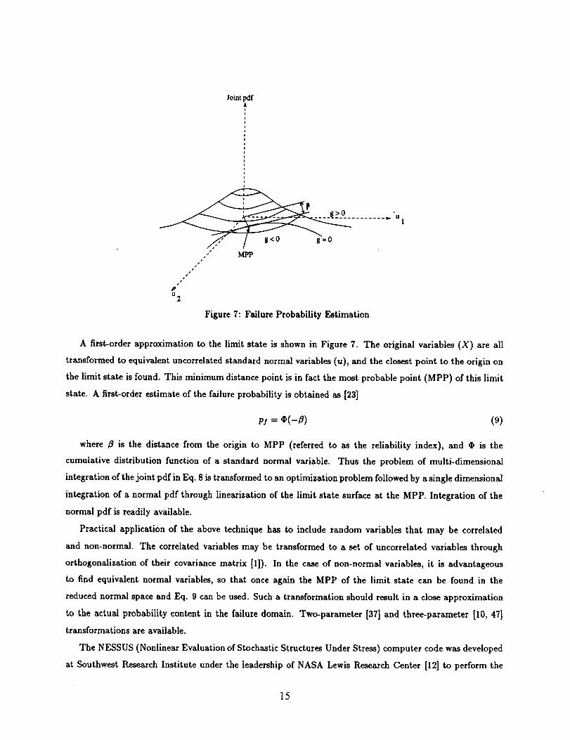
Figure 7: Failure Probability Estimation
A first-order approximation to the limit state is shown in Figure 7. The original variables (X) are all
transformed to equivalent uncorrelated standard normal variables (u), and the closest point to the origin on
the limit state is found. This minimum distance point is in fact the most probable point (MPP) of this limit
state. A first-order estimate of the failure probability is obtained as [23]
Pl = ¢(-_) (9)
where /_is the distance from the originto MPP (referredto as the reliabilityindex), and _ isthe
cumulative distributionfunction of a standard normal variable. Thus the problem of multi-dimensional
integrationofthejointpdf inEq. 8 istransformedto an optimizationproblem followedby a singledimensional
integration of a normal pdf through linearization of the limit state surface at the MPP. Integration of the
normal pdf is readily available.
Practical application of the above technique has to include random variables that may be correlated
and non-normal. The correlated variables may be transformed to a set of uncorrelated variables through
orthogonalization of their covariance matrix [1]). In the case of non-normal variables, it is advantageous
to find equivalent normal variables, so that once again the MPP of the limit state can be found in the
reduced normal space and Eq. 9 can be used. Such a transformation should result in a close approximation
to the actual probability content in the failure domain. Two-parameter [37] and three-parameter [10, 47]
transformations are available.
The NESSUS (Nonlinear Evaluation of Stochastic Structures Under Stress) computer code was developed
at Southwest Research Institute under the leadership of NASA Lewis Research Center [12] to perform the
15
probabilistic analysis of select space shuttle main engine components. It uses the refined three-parameter
equivalent normal transformation scheme of Wu and Wirsching [47]. However, instead of performing many
iterations to search for the exact minimum distance point, NESSUS employs an Advanced Mean Value
(AMV) procedure [49] to obtain sufficient accuracy in the second iteration. The search begins by computing
the sensitivities of the performance function at the mean values of the random variables, and using these
sensitivities to obtain a mean value first order (MVFO) estimate of the MPP and failure probability. Re-
analysis at this point provides the correct value of the performance function at this point. This information,
combined with that from the MVFO analysis, is seen to provide an accurate AMV estimate of the failure
probability. Further refinements are also possible, if necessary. The AMV analysis has been verified for
numerous problems using Monte Carlo simulation and has been found to provide accurate and fast estimates
of failure probability for practical space shuttle main engine (SSME) hardware [11] [38].
Perhaps the most significant contribution of the limit state modeling technique is the computation of
sensitivities of structural reliability to the basic random parameters. The sensitivity of the reliability index
to the original random variables Xi can be computed as
= out (10)Xi _ cgu.i OXij=l
where uj's are the equivalent uncorrelated standard normal variables. The first term in the summation is
obtained from the direction cosines of the MPP vector, and the second term is obtained from the transfor-
mation from the X-space to the u-space. This sensitivity measure combines both the physical sensitivities
and the uncertainty of the random variables.
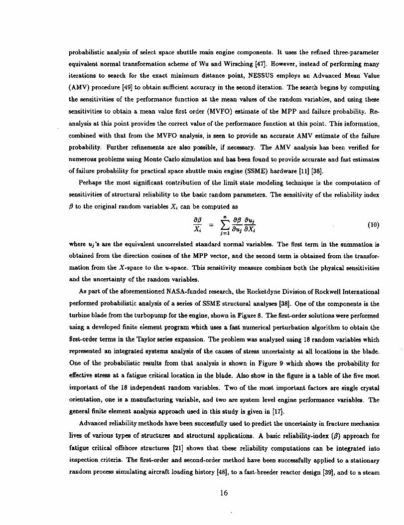
As part of the aforementioned NASA-funded research, the Rocketdyne Division of Rockwell International
performed probabilistic analysis of a series of SSME structural analyses [38]. One of the components is the
turbine blade from the turbopump for the engine, shown in Figure 8. The first-order solutions were performed
using a developed finite element program which uses a fast numerical perturbation algorithm to obtain the
first-order terms in the Taylor series expansion. The problem was analyzed using 18 random variables which
represented an integrated systems analysis of the causes of stress uncertainty at all locations in the blade.
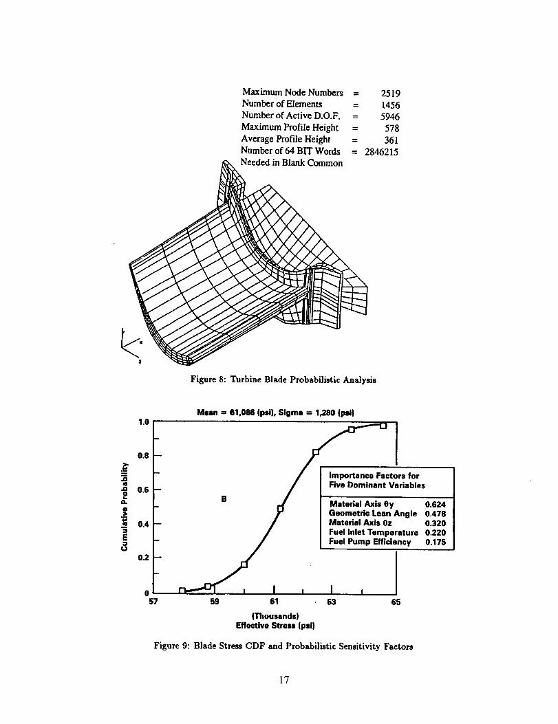
One of the probabilistic results from that analysis is shown in Figure 9 which shows the probability for
effective stress at a fatigue critical location in the blade. Also show in the figure is a table of the five most
important of the 18 independent random variables. Two of the most important factors are single crystal
orientation, one is a manufacturing variable, and two are system level engine performance variables. The
general finite element analysis approach used in this study is given in [17].
Advanced reliability methods have been successfully used to predict the uncertainty in fracture mechanics
lives of various types of structures and structural applications. A basic reliability-index (_ff) approach for
fatigue critical offshore structures [21] shows that these reliability computations can be integrated into
inspection criteria. The first-order and second-order method have been successfully applied to a stationary
random process simulating aircraft loading history [48], to a fast-breeder reactor design [39], and to a steam
16
Maximum Node Numbers
Number of Elements
Number of Active D.O.F.
Maximum Profile Height
Average lh'of'de HeightNumber of 64 BIT Words
Needed in Blank Common
= 2519
= 1456
= 5946
= 578
= 361
= 2846215
Figure 8: Turbine Blade Probabilistic Analysis
.nq
.Q
oQ.
@
m
E
¢J
1.0
0.8
0.8
m
I
m
0.4
0.2 --
057
Mean = 01,086 (psi), Sigma -- 1,280 (psi}
_ctors for
/ Five Dominant VariablesB ,/ "o. 4
y Geometric Lean Angle 0.478/ Material Axis Oz 0.320
jf Fuel Inlet Temperature 0.220
59 61 63 65
(Thousands)Effective Stress (psi)
Figure 9: Blade Stress CDF and Probabilistic Sensitivity Factors
17
turbine design [41]. A summary of an updating algorithm to improve solution accuracy developed by the
NASA-funded research [49] was shown to be effective for fracture mechanics analysis [45]. A special finite
element approach to probabilistic fracture mechanics is given in [6] which is also based on the limit state
approach.
Part II of this paper describes in detail the application of the limit state modeling methodology to the
engine structures fracture reliability problem.
3 System Failure
The probabilistic estimation of fracture life of mechanical components also has to contend with issues such
as multiple possible sites of crack initiation, the rate at which the initiated cracks grow at different sites, the
probability of coalescence of two or more cracks, several possible crack propagation paths, etc. This becomes
a system reliability problem.
Traditionally, mechanical system reliability has been based on classical statistics and experimental ob-
servations, and concepts such as MTBF and Weibull or exponential life distribution. In addition to the
inadequacies of such an approach in linking component and system reliability to design decisions, increas-
ingly complex propulsion systems are making it uneconomical to continue this approach due to the high cost
involved in testing. Therefore the limit state modeling approach has been extended by the authors to system
reliability evaluation of gas turbine engine structures. System failure may occur due to a combination of any
of the individual component failure modes. Structural system reliability analysis has traditionally modeled
structures as networks of simple parallel and series components analogous to electrical circuits. A "series"
or weakest-link system is one in which the violation of any one of the design limit states causes system
failure. In this case, the probability of system failure is computed through the union of the individual failure
events. A "parallel" or redundant or fail-safe system is one in which system failure occurs only when all
the individual modes are violated. In this case, the probability of system failure is the probability of joint
occurence (intersection) of all the individual failure events.
For systems with a large number of components, it is difficult to accurately compute the joint proba-
bilities of three or more failure events, except through Monte Carlo simulation. Therefore, first-order and
second-order analytical bounds for the system failure probability have been derived, e.g., [18]. First-order
approximations to the joint probabilities of multiple failure events have also been derived [20]. Monte Carlo
simulation has been the tool of choice for large complex systems which consist of many components and
failure paths. Efficient sampling schemes have been developed in this regard [25, 46].
System reliability estimation of mechanical structures such as in gas turbine engines also has to consider
the fact that some failure modes such as yielding, fracture, creep etc. are progressive in nature and distributed
over a continuum. Some of the failure modes may be physically related to each other; in that case the
probability of failure in one mode as the structure undergoes progressive damage in another is of concern.
18
mj=O
mj>O
mi=O
Ini>o /
i/j
_j/i
Oz i gin
ij =
_i/j ffi
x/l- pi_
_i'Pij_j
V -p j
Figure 10: Joint Probability of Two Failure Modes
A structural reanalysis procedure has recently been developed to accurately estimate the failure probability
various critical failure modes affected by progressive damage [13, 31].
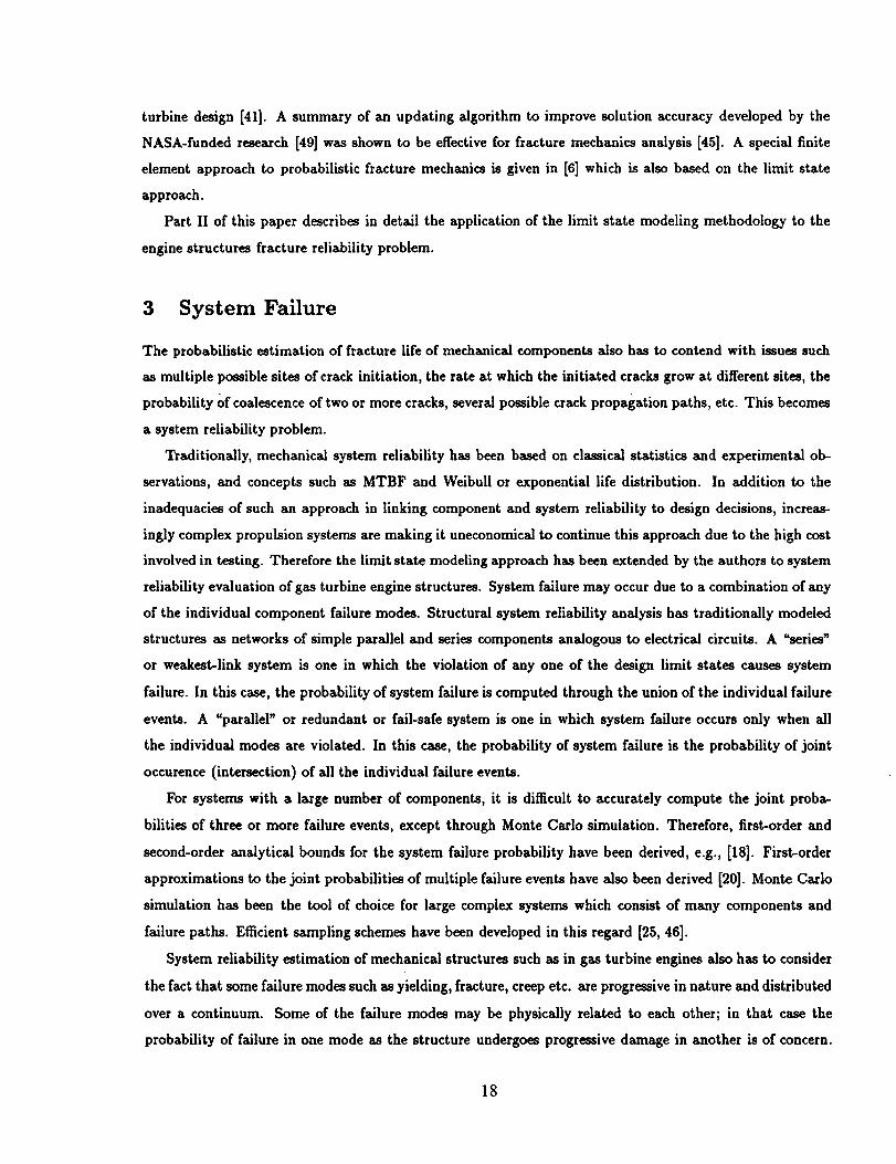
System reliability analysis with the limit state modeling approach also results in the computation of
overall system sensitivities to the random variables. For example, a first-order approximation to the system
sensitivity factors may be computed as
OXj i=, OXj (11)
where p} is the overall system failure probability, p) is the ith mode failure probability, Xj is ]th random
variable, and m is the number of individual failure modes. This result applies to the case where the system
failure is the union of the individual failures, and is based on the chain rule of differentiation applied to the
first-order upper bound of the probability of the union.
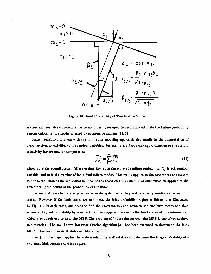
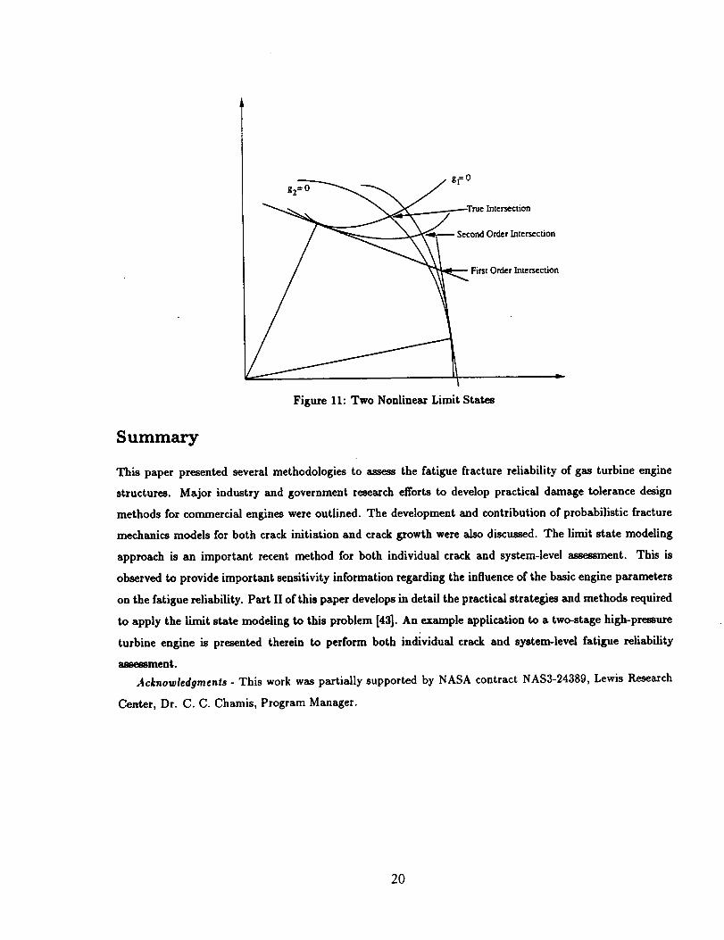
The method described above provides accurate system reliability and sensitivity results for linear limit
states. However, if the limit states are nonlinear, the joint probability region is different, as illustrated
by Fig. 11. In such cases, one needs to find the exact intersection between the two limit states and then
estimate the joint probability by constructing linear approximations to the limit states at this intersection,
which may be referred to as a joint MPP. The problem of finding the correct joint MPP is one of constrained
minimization. The well-known Rackwitz-Fiessler algorithm [37] has been extended to determine the joint
MPP of two nonlinear limit states as outlined in [30].
Part II of this paper applies the system reliability methodology to determine the fatigue reliability of a
two-stage high pressure turbine engine.
19
,2 j, 0TrueIntersection
Figure II: Two Nonlinear Limit States
Summary
This paper presented several methodologies to assess the fatigue fracture reliability of gas turbine engine
structures. Major industry and government research efforts to develop practical damage tolerance design
methods for commercial engines were outlined. The development and contribution of probabilistic fracture
mechanics models for both crack initiation and crack growth were also discussed. The limit state modeling
approach is an important recent method for both individual crack and system-level assessment. This is
observed to provide important sensitivity information regarding the influence of the basic engine parameters
on the fatigue reliability. Part II of this paper develops in detail the practical strategies and methods required
to apply the limit state modeling to this problem [43]. An example application to a two-stage high-pressure
turbine engine is presented therein to perform both individual crack and system-level fatigue reliability
assessment.
Acknowledgments - This work was partially supported by NASA contract NAS3-24389, Lewis Research
Center, Dr. C. C. Chamis, Program Manager.
2O
References
[1] A. H.-S Ang and W. H. Tang, Probability Concepts in Engineering Planning and Design, Vol
2, John Wiley and Sons, New York, 1984.
[2] Anon., _Probabilistic/Fracture-Mechanics Model for Service Life", NASA Tech Briefs MFS-27237.
[3] Anon., U. S. Air Force, Military Standard MIL-STD-1783, 1984.
[4] Hiroo Asada, "Reliability assessment of pressurized fuselages with multiple-site fatigue cracks", Pro-
ceedings of the 5 t_ International Conference on Structural Safety and Reliability, 1989, pp.
2369-2372.
[5] P. M. Besuner, "Probabilistic fracture mechanics", in Probabillstic Fracture Mechanics and Re-
liability, ed. J. W. Provan, op. cit., pp. 387-436.
[6] G. H. Besterfield, W. K. Liu, M. A. Lawrence, and T. B. Belytschko, "Brittle fracture reliability by
probabilistic finite elements", Journal of Engineering Mechanics, Vol. 116, No. 3, ASCE, 1990,
pp. 642-659.
[7] V. V. Bolotin, "Theory of extremes and its applications to mechanics of solids and structures", Pro-
ceedings of the 1Jt World Congress of the Bernoulli Society, Tashkent, USSR, ed. by Yu. A.
Prohorov and V. V. Sazanov, Utrecht, The Netherlands, VNU Science Press, 1987.
[8] A. Briickner, "Numerical methods in probabilistic fracture mechanics", in Probabilistic Fracture
Mechanics and Reliability, ed. J. W. Provan, op. cit., pp. 351-386.
[9] A. Briickner-Foit, H. Jgckels, H. Lahodny, and D. Munz, _Fatigue reliability of components containing
microstructural flaws", Proceedings of the 5 th International Conference on Structural Safety
and Reliability, 1989, pp. 1499-1506.
[10] X. Chen and N. C. Lind, "Fast Probability Integration by Three-Parameter Normal Tail Approxima.
tion',Structural Safety, Vol. 1, pp. 269-276, 1983.
[11] T. A. Cruse, O. H. Burnside, Y.-T Wu, E. Z. Polch, and J. B. Dias, "Probabilistic Structural Analy-
sis Methods for Select Space Propulsion System Structural Components (PSAM)', Computers and
Structures, Vol. 29(5), pp. 891-901, 1988.
[12] T. A. Cruse, C. C. Chamis, and Millwater, H.R., "An Overview of the NASA(LeRC)-SwRI Proba-
bilistic Structural Analysis (PSAM) Program", Proceedings, 5th International Conference on
Structural Safety and Reliability (ICOSSAR), San Francisco, California, pp. 2267-2274, 1989.
21
[13] T. A. Cruse, Q. Huang, S. Mehta, and S. Mahadevan, "System Reliability and Risk Assessment," Pro-
ceedlngs of the 33rd AIAA/ASME/ASCE/AHS/ASC Conference on Structures, Struc-
tural Dynamics and Materials, Dallas, Texas, pp.424-431, 1992.
[14] T. A. Cruse and T. G. Meyer, "A cumulative fatigue damage model for gas turbine disks subject to
complex mission loading" ,Journal of Engineering for Power, Vol. 101, No. 4, 1979, pp. 563-571.
[15] T. A. Cruse and T. G. Meyer, "Low cycle fatigue life model for gas turbine engine disks", 3ournal of
Engineering Materials and Technology, Vol. 102, 1980, pp. 45-49.
[16] T. A. Cruse, "Engine components", in Practical Applications of Fracture Mechanics, NATO
AGARDograph #257, 1980, Chapter 2.
[17] T. A. Cruse, K. R. Rajagopal, and J. B. Diaz, "Probabilistic structural analysis methodology and ap-
plications to advanced space propulsion system components", Computing Systems in Engineering,
Vol. 1, Nos. 2-4, 1990, pp. 365-372.
[18] O. Ditlevsen, "Narrow Reliability Bounds for Structural Systems", Journal of Structural Mechanics,
VoL 3,453-472, 1979.
[19] N. Engsberg, C. G. Annis, Jr., and B. A. Cowles, Effects of Defects in Powder Metallurgy
Superalloys, AFWAL-TR-81-4191, Feb. 1982.
[20] S. Gollwitzer and R. Rackwitz, UAn efficient numerical solution to the multinormal integral _, Proba-
bilistic Engineering Mechanics, Vol. 3(2), 1988, pp. 98-101.
[21] Guoyang Jiao and Torgeir Moan, "Reliability-based fatigue and fracture design criteria for welded
offshore structures", Engineering Fracture Mechanics, Vol. 41, No. 2, 1992, pp. 271-282.
[22] J. A. Harris, Jr. and R. White, Engine Component Retirement for Cause, AFWAL-TR-87-4069,
August 1987.
[23] A. M. Hasofer and N. C. Lind, "Exact and Invariant Second Moment Code Format", Journal of the
Engineering Mechanics Division, ASCE, Vol 100, No.EM1, pp. 111-121, 1985
[24] Peter W. Hovey and Alan P. Berens, "Statistical evaluation of NDE reliability in the aerospace industry",
Review of Progress in Quantitative NDE, Vol. 7B, 1988, pp. 1761-1768.
[25] A. Karamchandani, "Structural System Reliability Analysis Methods," Report No. 83, John A. Blume
Earthquake Engineering Center, Stanford University, 1987.
[26] T. T. King, W. D. Cowie, and W. H. Reimann, "Damage Tolerance Design Concepts for Military
Engines," Proceedings No. 393, AGAItD Conference on Damage Tolerance Concepts for
Critical Engine Components, 1985.
22
[27]P.Kittl and G. Diaz, "Five deductions of Weibull's distribution function in the probabilistic strength
of materials", Engineering Fracture Mechanics, Vol. 36, No. 5, 1990, pp. 749-762.
[28] P. Kittl and G. Diaz, "Size effect on fracture strength in the probabilistic strength of materials",
Reliability Engineering and System Safety_ Vol. 28, 1990. pp. 9-21.
[29] P. E. Magnusen, A. J. Hinkle, W. T. Kaiser, R. J. Bucci, and R. L. Roll, "Durability assessment based
on initial material quality", Journal of Testing and Evaluation, Vol. 18, No. 6, 1990, pp. 439-445.
[30] S Mahadevan, and T. A. Cruse,'An Advanced First-Order Method for System Reliability", Proceed-
ings of the ASCE Joint Specialty Conference on Probabilistlc Mechanics and Structural
and Geotechnical Reliability, Denver, Colorado, pp. 487-490, 1992.
[31] S. Mahadevan, T. A. Cruse, Q. Huang, and A. Mehta, "Structural Reanalysis for System Reliability
Computation,"in Reliability Technology, ASME AD-28, ed. by T.A. Cruse, American Soc. of Mech.
Engrs, New York, pp. 169-188, 1992.
[32] W. Scott Martin and Paul Wirsching, "Fatigue crack initiation - propagation reliability model", Journal
of Materials in Civil Engineering, Vol. 3, No. 1, 1991, pp. 1-18.
[33] L. N. McCartney, "Extensions of a statistical approach to fracture", International Journal of Frac-
ture_ Vol. 15, No. 5, 1979, pp. 477-487.
[34] Liao Min and Yang Qing-Xiong, "A probabilistic model for fatigue crack growth", Engineering Frac-
ture Mechanics_ Vol. 43, No. 4, 1992, pp. 651-655.
[35] B. Palmberg, A. F. Blom, and S. Eggwertz, "Probabilistic damage tolerance analysis of aircraft struc-
tures", in Probabillstic Fracture Mechanics and Reliability, ed. J. W. Provan, op. cit., pp.
47-130.
[36] James W. Provan, Editor of Probabilistic Fracture Mechanics and Reliability, Martinus Nijhoff
Publishers, Dordrecht, The Netherlands, 1987.
[37] R. Rackwitz and B. Fiessler, "Structural Reliability Under Combined Random Load Sequences", Com-
puters and Structures, Vol. 9, No. 5, pp. 484-494, 1978.
[38] K.R. Rajagopal, A. Debchaudhury and J.F. Newell, "Verification of NESSUS Code on Space Propulsion
Components", Proceedings, 5th International Conference on Structural Safety and Reliabil-
ity_ ICOSSAR '89, San Francisco, California, pp. 2299-2306, 1989.
[39] H. Riesch-Oppermann, and A. Briickner-Foit, "First- and second-order approximations of failure prob-
abilities in probabilistic fracture mechanics, Reliability Engineering and System Safety, Vol. 23,
1988, pp. 183-194.
23
[40] J. L. Rudd, J. N. Yang, S. D. Manning, and G. W. Lee, "Probabilistic fracture mechanics analysis
methods for structural durability", Proceedings of AGARD Meeting on Behavior of Short
Cracks in Airframe Components, Toronto, Canada, 1982.
[41] Murari P. Singh, "Reliability evaluation of a weld repaired steam turbine rotor using probabilistic
fracture mechanics", Design, Repair, and Refurbishment of Steam Turbines, PWR-VoL 113,
ASME, 1991, pp. 255-259.
[42] K. Sobczyk, "Stochastic models for fatigue damage of materials", Advanced Applications of Prob-
ability, Vol. 19, 1987, pp. 652-673.
[43] R. G. Tryon, S. Mahadevan, and T. A. Cruse, "Fatigue Reliability of Gas Turbine Engine Structures:
Part II.-- Limit State Modeling", Engineering _'_racture Mechanics, under review.
[44] T. Watkins, Jr. and C. G. Annis, Jr., Engine Component Retirement for Cause: Probabillstic
Life Analysis Technique, AFWAL-TR-85-4075, June 1985.
[45] P. H. Wirsching, T. Y. Torng, and W. S. Martin, "Advanced fatigue reliability analysis", International
Journal of Fatigue, Vol. 13, No. 5, 1991, pp. 389-394.
[46] Wu, Y.-T., "An Adaptive Importance Sampling Method for Structural System Reliability Analysis,"in
Reliability Technology, ASME AD-28, ed. by T.A. Cruse, American Soc. of Mech. Engrs, New York,
pp. 217-232, 1992.
[47] Y.-T. Wu and P. H. Wirsching, "New algorithm for structural reliability estimation", Journal of
Engineering Mechanics, Vol. 113, No. 9, ASCE, pp. 1319-1336.
[48] Y.-T. Wu, O. H. Burnside, and J. Dominguez, "Efficient probabilistic fracture mechanics analysis",
Numerical Methods in Fracture Mechanics, Proceedings of the Fourth International Con-
ference, Ed. A. R. Luxmore, D. R. J. Owen, Y. P. S. Rajapakse, and M. F. Kanninen, San Antonio,
Texas, 1987.
[49] Y.-T. Wu, H. R. Millwater, and T. A. Cruse, "An advanced probabilistic structural analysis method for
implicit performance functions", AIAA Journal, Vol. 28, No. 9, 1990, pp. 1663-1669.
[50] W. Weihull, "A statistical distribution function of wide applicability" ,Journal of Applied Mechanics,
VoL 18, 1951.
[51] J. N. Yang, S. D. Manning, and J. L. Rudd, "Evaluation of a stochastic initial fatigue quality model
for fastener holes", Fatigue in Mechanically Fastened Composite and Metallic Joints, ASTM
STP 927, Ed. John M. Potter, American Society for Testing and Materials, Philadelphia, PA, 1986,
pp. 118-149.
24
[52] J. N. Yang, W. H. Hsi, S. D. Manning, and J. L. Rudd, "Stochastic crack growth models for applications
to aircraft", in Probabillstic Fracture Mechanics and Reliability, ed. J. W. Provan, op. cit., pp.
171-212.
[53] J. N. Yang and S. D. Manning, "Application of probabilistic approach for crack growth damage accu-
mulation in metallic structures", Proceedings of the 5th International Conference on Structural
Safety and Reliability, 1989, pp. 1475-1482.
[54] J. N. Yang and S. D. Manning, "Demonstration of probabilistic-based durability method for metallic
airframes", Journal of Aircraft, Vol. 27, No. 2, 1990, pp. 169-175.
25
Part II - A CASE STUDY
Summary
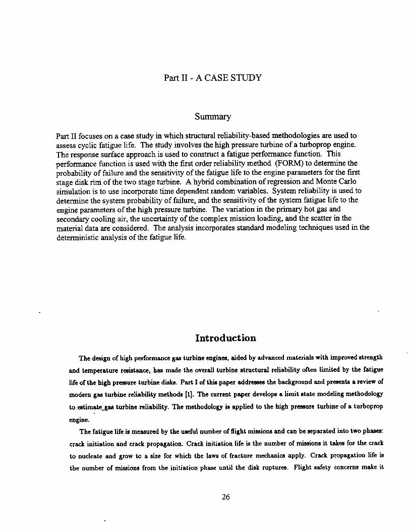
Part II focuses on a case study in which structural reliability-based methodologies are used to
assess cyclic fatigue life. The study involves the high pressure turbine of a turboprop engine.
The response surface approach is used to construct a fatigue performance function. This
performance function is used with the first order reliability method (FORM) to determine the
probability of failure and the sensitivity of the fatigue life to the engine parameters for the first
stage disk rim of the two stage turbine. A hybrid combination of regression and Monte Carlo
simulation is to use incorporate time dependent random variables. System reliability is used to
determine the system probability of failure, and the sensitivity of the system fatigue life to the
engine parameters of the high pressure turbine. The variation in the primary hot gas and
secondary cooling air, the uncertainty of the complex mission loading, and the scatter in the
material data are considered. The analysis incorporates standard modeling techniques used in the
deterministic analysis of the fatigue life.
Introduction
The design of high performance gas turbine engines, aided by advanced materials with improved strength
and temperature resistance, has made the overall turbine structural reliability often limited by the fatigue
life of the high pressure turbine disks. Part I of this paper addresses the background and presents a review of
modern gas turbine reliability methods [1]. The current paper develops a limit state modeling methodology
to estimate.gu turbine reliability. The methodology is applied to the high pressure turbine of a turboprop
engine.
The fatigue life is measured by the useful number of flight missions and can be separated into two phases:
crack initiation and crack propagation. Crack initiation life is the number of missions it takes for the crack
to nucleate and grow to a size for which the laws of fracture mechanics apply. Crack propagation life is
the number of missions from the initiation phase until the disk ruptures. Flight safety concerns make it
26
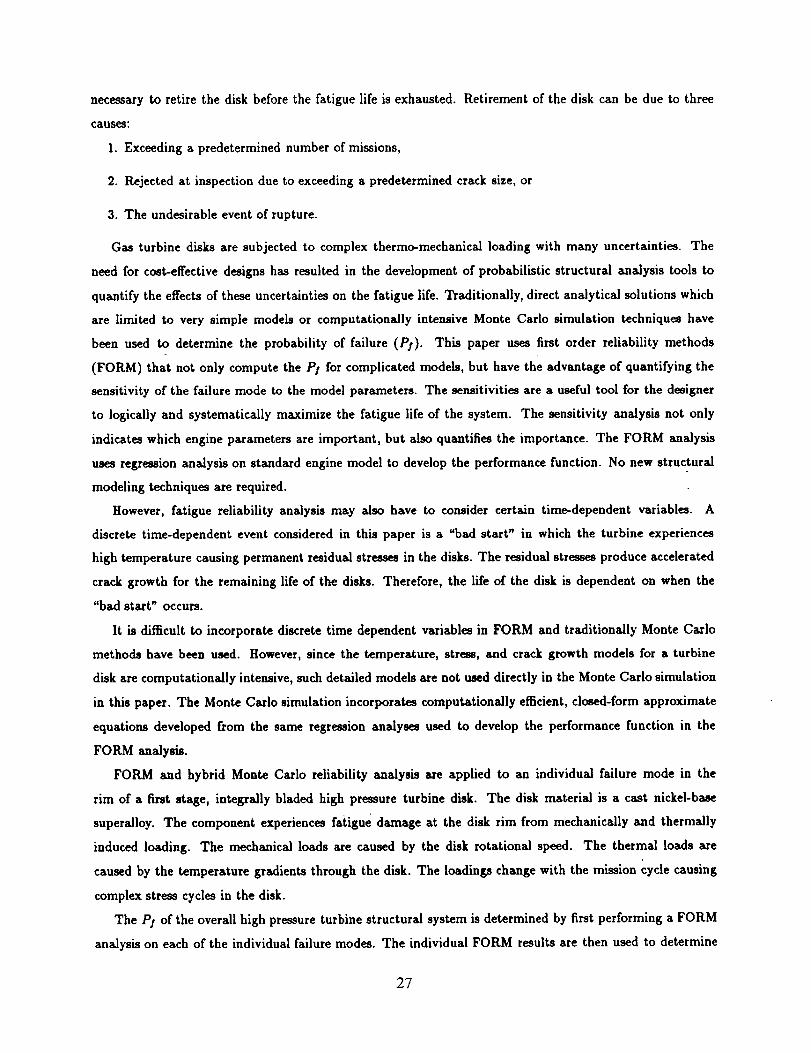
necessary to retire the disk before the fatigue life is exhausted. Retirement of the disk can be due to three
causes:
1. Exceeding a predetermined number of missions,
2. Rejected at inspection due to exceeding a predetermined crack size, or
3. The undesirable event of rupture.
Gas turbine disks are subjected to complex thermo-mechanical loading with many uncertainties. The
need for cost-effective designs has resulted in the development of probabilistic structural analysis tools to
quantify the effects of these uncertainties on the fatigue life. Traditionally, direct analytical solutions which
are limited to very simple models or computationally intensive Monte Carlo simulation techniques have
been used to determine the probability of failure (Pl). This paper uses first order reliability methods
(FORM) that not only compute the P! for complicated models, but have the advantage of quantifying the
sensitivity of the failure mode to the model parameters. The sensitivities are a useful tool for the designer
to logically and systematically maximize the fatigue life of the system. The sensitivity analysis not only
indicates which engine parameters are important, but also quantifies the importance. The FORM analysis
uses regression analysis on standard engine model to develop the performance function. No new structural
modeling techniques are required.
However, fatigue reliability analysis may also have to consider certain time-dependent variables. A
discrete time-dependent event considered in this paper is a "bad start" in which the turbine experiences
high temperature causing permanent residual stresses in the disks. The residual stresses produce accelerated
crack growth for the remaining life of the disks. Therefore, the life of the disk is dependent on when the
"bad start" occurs.
It is difficult to incorporate discrete time dependent variables in FORM and traditionally Monte Carlo
methods have been used. However, since the temperature, stress, and crack growth models for a turbine
disk are computationally intensive, such detailed models are not used directly in the Monte Carlo simulation
in this paper. The Monte Carlo simulation incorporates computationally efficient, closed-form approximate
equations developed from the same regression analyses used to develop the performance function in the
FORM analysis.
FORM and hybrid Monte Carlo reliability analysis are applied to an individual failure mode in the
rim of a first stage, integrally bladed high pressure turbine disk. The disk material is a cast nickel-base
superalloy. The component experiences fatigue damage at the disk rim from mechanically and thermally
induced loading. The mechanical loads are caused by the disk rotational speed. The thermal loads are
caused by the temperature gradients through the disk. The loadings change with the mission 'cycle causing
complex stress cycles in the disk.
The P! of the overall high pressure turbine structural system is determined by first performing a FORM
analysis on each of the individual failure modes. The individual FORM results are then used to determine
27
the systemfailureprobabilitythroughtheunionof individualmodefailures.Themethodalsoprovides
sensitivity information on the individual and system failure modes.
The approach presented considers the inherent scatter and the random nature of the engine operation,
hardware and material data. The methodology can be described along the following steps:
1. Determine potentially significant random variables.
2. Use engine system and structural finite element models to determine temperatures and stresses.
3. Use crack initiation and crack propagation models to determine fatigue life.
4. Use FORM analysis to determine P! and the sensitivities of individual failure modes (without time-
dependent random variables).
5. Use hybrid Monte Carlo analysis to determine P/ of individual failu_ modes (with time-dependent
random variables).
6. Use the system reliability method to determine P! and the sensitivities of the system failure (without
time-dependent random variables).
1 Performance Function
The performance function is generally defined as
g(x) = l(xt, x2,..., x,) (1)
where g(X) is a closed form function of the random variables Xz, X2,..., X,. The performance function
representing the onset of fatigue in gas turbine engines, g(X), is taken to be the number of flight cycles to
failure. To develop the performance function, the potentially significant random variables must be identi-
fied. Perturbation analysis is performed to eliminate the random variables that do not significantly effect
the fatigue life. Regression analysis is performed on the perturbation results to develop an closed form
approximation to g(X).
1.1 Determining Potentially Significant Random Variables
Ideally, all random variables should be measurable basic engine parameters. The random variables should
be physically measurable, because the scatter must be known. The random variables should be primitive
independent parameters such that the correlation between variables is minimized. The mean value, standard
deviation, and distribution type must be estimated based on test data or sound engineering experience.
Although all physically measured parameters have some variability, some physically measured parameters
can be considered deterministic variables while others must be considered random variables. A variable can
28
be considered deterministic if the range of variability is small enough such that any value within the range
will not significantly affect the outcome of the modeled response. A variable must be considered random if
range of variability is large enough such that changing the value within the range affects the response.
As a first step, engineering judgment should be used to determine which variable might be random. When
in doubt, the variable should be considered random. Then a sensitivity analysis in which the response is
modeled for the extreme values of the range of the variable in question should be performed. If the analysis
shows the sensitivity to this variable to be low, then the variable can be considered deterministic. Care
must be taken to reduce the number of random variables to as few as necessary because a major effort of
probabilistic modeling is in determining the statistics of the random variables.
It is necessary to determine all of the engine parameters that affect fatigue life. In a complex system such
as a gas turbine engine, it is quite difficult to understand the details as to which parameters affect disk life
and exactly how these parameters interact. Detailed knowledge of each discipline and how each influences
the disk response is needed. The disciplines that influence disk life include: primary hot gas flow, secondary
cooling air flow, heat transfer, structural mechanics, life prediction, materials, inspection, failure analysis
and design. Input from experienced engineers from all of the above disciplines was used to identify eleven
potentially significant random variables. These included the burner outlet temperatures (BOT), burner
profile, dwell times, seal clearances, material properties, and the number of missions at which the disk is
retired. The following sections discuss the use of engine models to perform sensitivity analysis which showed
the response to be sensitive to five of the eleven potentially significant random variables.
1.2 Engine Models
The present analysis incorporates the same basic engine models used in the deterministic fatigue life analysis.
No new modeling techniques are needed. However, the models are combined in a manner that allows the
designer to gain more understanding than what is available though a deterministic analysis. The basic
models used in the analysis are briefly described below.
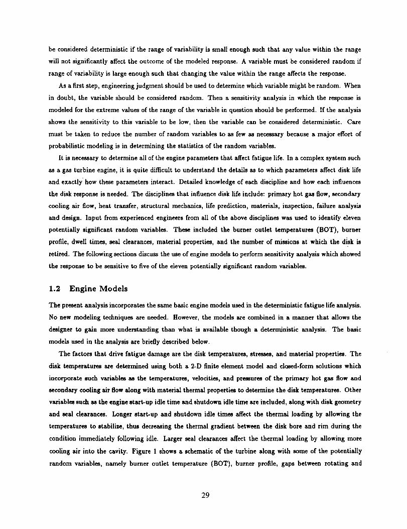
The factors that drive fatigue damage are the disk temperatures, stresses, and material properties. The
disk temperatures are determined using both a 2-D finite element model and clewed-form solutions which
incorporate such variables as the temperatures, velocities, and pressures of the primary hot gas flow and
secondary cooling air flow along with material thermal properties to determine the disk temperatures. Other
variables such as the engine start-up idle time and shutdown idle time are included, along with disk geometry
and seal clearances. Longer start-up and shutdown idle times affect the thermal loading by allowing the
temperatures to stabilize, thus decreasing the thermal gradient between the disk bore and rim during the
condition immediately following idle. Larger seal clearances affect the thermal loading by allowing more
cooling air into the cavity. Figure 1 shows a schematic of the turbine along with some of the potentially
random variables, namely burner outlet temperature (BOT), burner profile, gaps between rotating and
29
DIGINE VARIABLES
Burner Outlet
Temperature (BOT]
Gas Stream
Temperature
Profile
Aft Axial Gap
Seal Leakage
MISSIGN VARIABLES
Maximum Start-up SOT
Start-up Dwell
Shutdown Dwell
ow - J - J
LIFE VARIABLES
Crack Initiation Life
Initial Crack Size
Number of Initiation sites
Crack Growth Rate
Figure 1: Engine Model Random Variables
stationary parts, and seal leakages. Other variables in the heat transfer model such as idle dwell times are
also treated as random variables.
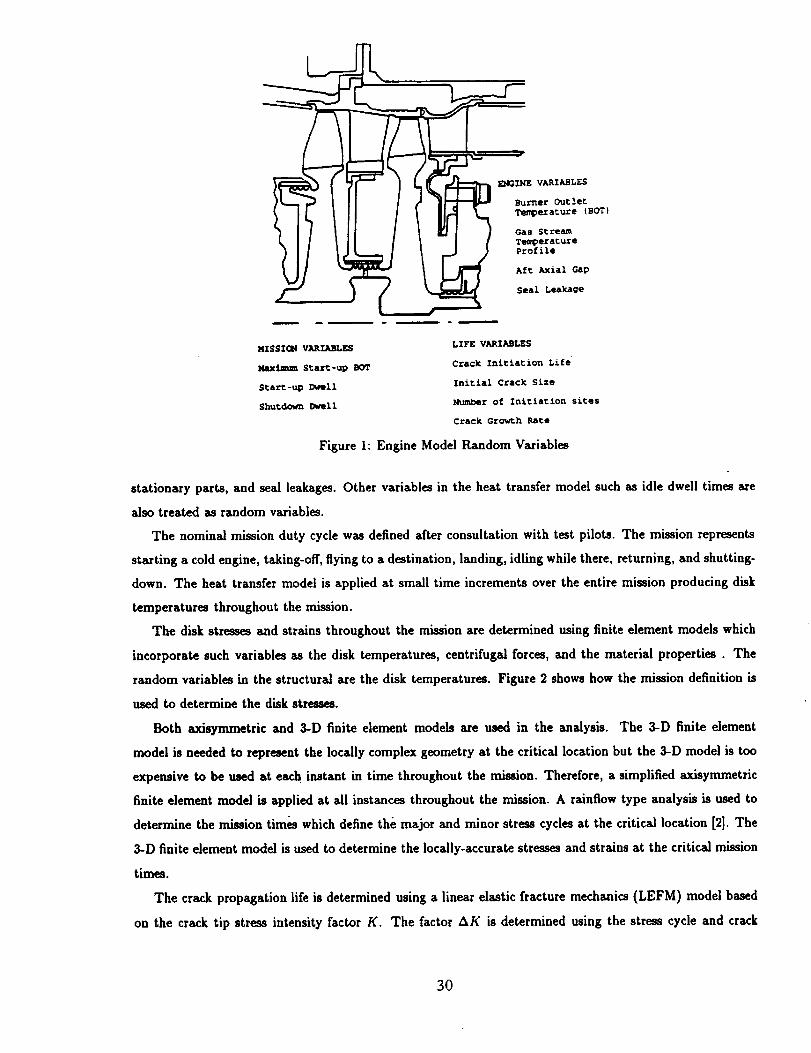
The nominal mission duty cycle was defined after consultation with test pilots. The mission represents
starting a cold engine, taking-off, flying to a destination, landing, idling while there, returning, and shutting-
down. The heat transfer model is applied at small time increments over the entire mission producing disk
temperatures throughout the mission.
The disk stresses and strains throughout the mission are determined using finite element models which
incorporate such variables as the disk temperatures, centrifugal forces, and the material properties. The
random variables in the structural are the disk temperatures. Figure 2 shows how the mission definition is
used to determine the disk stresses.
Both axisymmetric and 3-D finite element models are used in the analysis. The 3-D finite element
model is needed to represent the locally complex geometry at the critical location but the 3-D model is too
expensive to be used at each instant in time throughout the mission. Therefore, a simplified axisymmetric
finite element model is applied at all instances throughout the mission. A rainflow type analysis is used to
determine the mission times which define the major and minor stress cycles at the critical location [2]. The
3-D finite element model is used to determine the locally-accurate stresses and strains at the critical mission
times.
The crack propagation life is determined using a linear elastic fracture mechanics (LEFM) model based
on the crack tip stress intensity factor K. The factor AK is determined using the stress cycle and crack
3O
POWEI_
MISSION
DEFINITION
lime
TEMP
HEATTRANSFER
MODEL
WHEEL
TEMPERATURES
bore
STR UCTURA LMODEL
WHEELST_ES
a
Figure 2: Models Used at All Mission Points
geometry. The model considers disk geometry, initial crack size, and material data. Failure occurs when K
exceeds KIc. The Paris lawda
= C(AK)" (2)
is used to define the crack propagation at a given R and temperature, where _ is the crack growth rate,
AK is the stress intensity factor, and C,n are material constants. The maxima and minima of the stress
cycles computed from the mission analysis, the material constants, and the initial crack size are considered
random variables.
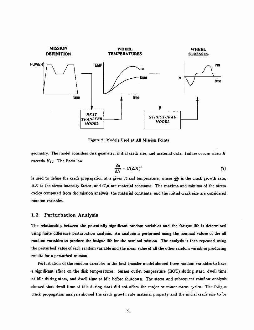
1.3 Perturbation Analysis
The relationship between the potentially significant random variables and the fatigue life is determined
using finite difference perturbation analysis. An analysis is performed using the nominal values of the all
random variables to produce the fatigue life for the nominal mission. The analysis is then repeated using
the perturbed value of each random variable and the mean value of all the other random variables producing
results for a perturbed mission.
Perturbation of the random variables in the heat transfer model showed three random variables to have
a significant affect on the disk temperatures: burner outlet temperature (BOT) during start, dwell time
at idle during start, and dwell time at idle before shutdown. The stress and subsequent rainflow analysis
showed that dwell time at idle during start did not affect the major or minor stress cycles. The fatigue
crack propagation analysis showed the crack growth rate material property and the initial crack size to be
31
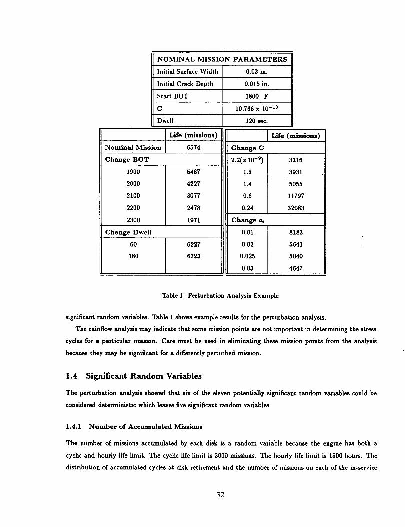
NOMINAL MISSION PARAMETERS
Initial Surface Width 0.03 in.
Initial Crack Depth 0.015 in.
Start BOT 1800 F
C 10.766 x I0 -x°
Dwell 120 sec.
I Life (missions)Nominal Mission 6574
Change BOT
1900
2000
5487
4227
l Life (missions)
Change C
2.2(x10 -9)
1.8
1.4
3216
3931
5055
2100
2200
2300
3077
2478
1971
Change Dwell
60
180
6227
6723
0.6
0.24
11797
32083
Change a_
0.01
0.02
0.025
0.03
8183
5641
5040
4647
Table h Perturbation Analysis Example
significant random variables. Table 1 shows example results for the perturbation analysis.
The rainflow analysis may indicate that some mission points are not important in determining the stress
cycles for a particular mission. Care must be used in eliminating these mission points from the analysis
because they may be significant for a differently perturbed mission.
1.4 Significant Random Variables
The perturbation analysis showed that six of the eleven potentially significant random variables could be
considered deterministic which leaves five significant random variables.
1.4.1 Number of Accumulated Missions
The number of missions accumulated by each disk is a random variable because the engine has both a
cyclic and hourly life limit. The cyclic life limit is 3000 missions. The hourly life limit is 1500 hours. The
distribution of accumulated cycles at disk retirement and the number of missions on each of the in-service
32
disks is determined from field service records. The histogram of the number of cycles on the retired disks
is added to the histogram of the number of cycles on the in-service disks to produce the histogram of total
fleet suspensions. The histogram of total fleet suspensions was approximated with a truncated Weibull
distribution.
1.4.2 BOT During Start
The BOT is a function of the duration the start switch is depressed by the pilot. The longer the pilot
depresses the switch the higher is the BOT. If the ambient temperature is cold, the engine is mistuned, or
the battery is low, the pilot may depress the switch for a long time resulting in high BOT. The high BOT
causes a thermal gradient across the disk which results in compressive yielding at the rim. The residual
effect of the yielding is to increase the R ratio (¢,nln/_rma=) of subsequent cyclic stresses. The high start
BOT affect the disk until a higher start BOT is experienced and the R ratio increases. There is little
information available concerning the occurrence of high start BOTs because start BOT is not recorded. The
range of possible start BOTs was divided into seven discrete temperatures for convenience. The probability
of occurrence of the discrete BOT for each start was estimated by interviewing the engine operators.
FORM analysis cannot account for a time dependent random variable such as start BOT. However, some
assumptions can be made about the start BOT that will allow the FORM analysis to compute an upper
bound on the P/. The worst case scenario is to determine the highest BOT the disk ever experiences and
assume the high BOT occurs on the first start.
Assume that the disk must endure 3000 missions. The probability of a disk experiencing a start BOT of
at least t in 3000 missions is
P,sooo= l - (1- Ptl)3°°° (3)
where Ptl is the probability of experiencing a BOT of at least t for each start.
The BOT distribution must be converted from a discrete distribution to a continuous distribution before
it can be used in FORM analysis. A polynomial curve fit is used to approximate the discrete distribution in
the standard normal (z,u) space
t - p_z - (4)cr|
u = -l(P(t < 7")) (5)
where z is the standard variable, u is the standard normal variable, t is the the value of the random variable
T representing the start BOT, @-1 is the the inverse of the standard normal transform and Pt, _t are the
mean and standard deviation of the start BOT.
The parameters p, and _, are estimated using the method of moments. The parameters z and u are
computed using Equations 4 and 5. By taking a polynomial curve fit of u in terms of z, the start BOT
33
distribution can be described by a function of the form
N
u = Ao + _., A,z _ (0)i---1
1.4.3 Dwell Time Before Shutdown
Longer idle dwell times affect the thermal loading by allowing the temperatures to stabilize, thus decreasing
the thermal gradient between the disk bore and rim during the shutdown. The dwell time distribution is
assumed to be lognormal. The distribution parameters were estimated by interviewing the engine operators.
1.4.4 Initial Crack Size
The crack initiation stage can be broken down into two stages: crack nucleation and small crack growth.
The stress concentrations of the complex geometry at the disk rim cause crack nucleation. In nickel-base
alloys, planar slip also causes crack nucleation even when no geometric stress concentration is present.
The second phase of crack initiation is the small crack growth phase. A small crack can be thought of as
a crack which is small compared to the microstructure. The conventionally cast nickel-based superalloy disk
has large grains. Therefore a physically large crack may still be considered microstructurally small because
the crack can lie in one or two grains. The crack growth rate of a small crack may vary widely, growing very
quickly and then retarding for thousands of cycles. Some cracks completely arrest. Grain size and resistance
at the grain boundary affect the small crack growth rate and are both random. In the large grain alloys,
a significant amount of the fatigue life can be spent in the small crack regime. A better understanding of
crack nucleation and the small crack effect is important in assessing disk fatigue life. Current research of the
authors investigates the random behavior of crack initiation.
The available crack initiation models are based on smooth round bar (SRB) tests. SRB tests of large
grain are such that after a crack nucleates, it progress to specimen failure in very few cycles. Consequently,
the SRB-based crack initiation models are not useful for determining crack growth in the small crack regime
but can be used to determine the cycles to crack nucleation. Comparison of the analytical strains from the
3-D stress analysis with the SRB test indicate that crack nucleation will occur in very few cycles.
The procedure in this paper is to assume a crack initiation life of zero cycles, and to choose a range of
initial equivalent flaw sizes (EIFS) based on the comparison of the analytical crack growth results with crack
size data from disks inspected in the field. The crack size does not represent the physically realized crack
initiation size, but is a crack in the LEFM regime that represents the culmination of crack nucleation and
the small crack effect. In other words, although the disk may not have a crack size of ai at zero cycles, the
crack growth analysis and field experience indicates that the disk "acts" as though it has a crack of size al
at zero cycles [3]. The initial crack size is found to fit a Weibull distribution.
The crack initiation size is not an independent random variable, but is highly correlated to start BOT
because crack initiation size is a function of the stress ratio R which is a function of start BOT. The FORM
34
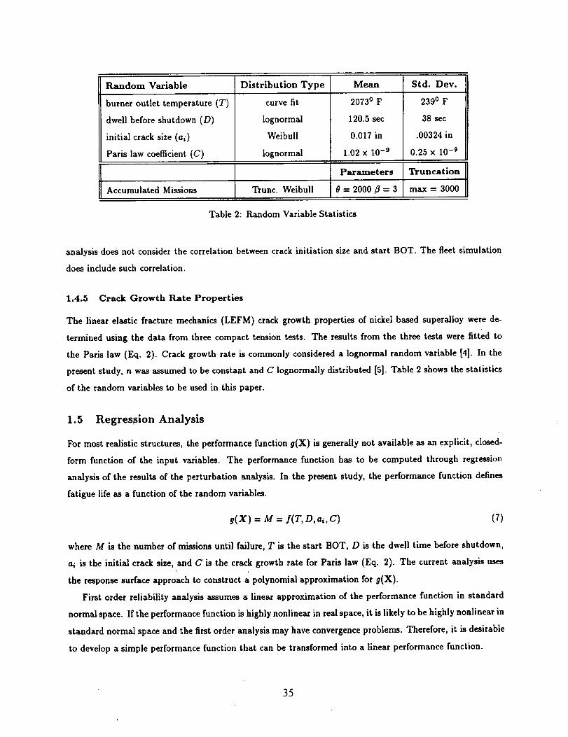
Random Variable Distribution Type Mean Std. Dev.
burner outlet temperature (T)
dwell before shutdown (D)
initial crack size (ai)
Paris law coefficient (C)
curve fit
lognormal
Weibull
lognormal
20730 F
120.5 sec
0.017 in
1.02 x 10 -9
2390 F
38 sec
.00324 in
0.25 × 10 -9
Parameters Truncation
Accumulated Missions Trunc. Weibull 0 = 2000/_ = 3 max = 3000
Table 2: Random Variable Statistics
analysis does not consider the correlation between crack initiation size and start BOT. The fleet simulation
does include such correlation.
1.4.5 Crack Growth Rate Properties
The linear elastic fracture mechanics (LEFM) crack growth properties of nickel based superalloy were de-
termined using the data from three compact tension tests. The results from the three tests were fitted to
the Paris law (Eq. 2). Crack growth rate is commonly considered a lognormal random variable [4]. In the
present study, n was assumed to be constant and C Iognormally distributed [5]. Table 2 shows the statistics
of the random variables to be used in this paper.
1.5 Regression Analysis
For most realistic structures, the performance function g(X) is generally not available as an explicit, closed-
form function of the input variables. The performance function has to be computed through regression
analysis of the results of the perturbation analysis. In the present study, the performance function defines
fatigue life as a function of the random variables.
g(X) = M - f(T, D, ai, C) (7)
where M is the number of missions until failure, T is the start BOT, D is the dwell time before shutdown,
ai is the initial crack size, and C is the crack growth rate for Paris law (Eq. 2). The current analysis uses
the response surface approach to construct a polynomial approximation for g(X).
First order reliability analysis assumes a linear approximation of the performance function in standard
normal space. If the performance function is highly nonlinear in real space, it is likely to be highly nonlinear in
standard normal space and the first order analysis may have convergence problems. Therefore, it is desirable
to develop a simple performance function that can be transformed into a linear performance function.
35
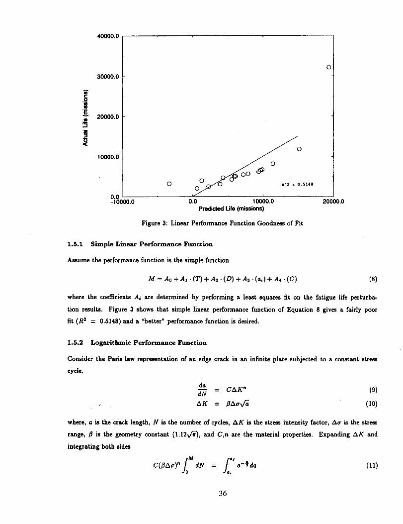
40000.0 , ,
30000.0
A
20000.0
10000.0
O
O
O O
oo _ .$148
0.0 10000.0
Predicted Ule (missions)
0.0-10000.0 20000.0
Figure 3: Linear Performance Function Goodness of Fit
1.5.1 Simple Linear Performance Function
Assume the performance function is the simple function
M = A0+ A_. (T) + A2- (D) + A3- Ca,)+ A,. (c) (8)
where the coefficients Ai are determined by performing a least squares fit on the fatigue life perturba-
tion results. Figure 3 shows that simple linear performance function of Equation 8 gives a fairly poor
fit (R _ = 0.5148) and a %etter" performance function is desired.
1.5.2 Logarithmic Performance Function
Consider the Paris law representation of an edge crack in an infinite plate subjected to a constant stress
cycle.
da
- OaK" (9)dN
AK = _:'_,V_ (,o)
where, a is the crack length, N is the number of cycles, AK is the stress intensity factor, Act is the stress
range, D is the geometry constant (1.12Vff), and C,n are the material properties. Expanding AK and
integrating both sides
C(BA_,)" dN - a-_da (11)i
36
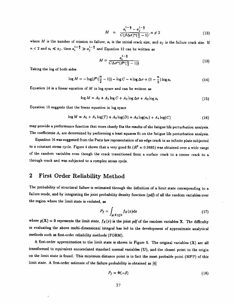
-M = C(3Aa)"(_- 1) 'n _ 2 (12)
where M is the number of mission to failure, ai is the initial crack size, and a I is the failure crack size. If
n < 2 and ai <(<(a], then _,a!-_ >> a_ -_ and Equation 12 can be written as
M - ai
CAtr"(/T'(_- 1)) (13)
Taking the log of both sides
n n
log M = - log(fl'*(_ - 1)) - logC - n logA_ + (1 loga, (14)
Equation 14 is a linear equation of M in log space and can be written as
logM = A0 + At IogC+ A2 log Ao" + Aa Iogai (15)
Equation 15 suggests that the linear equation in log space
log M = A0 + Al log(T) + A2 log(D) + A3 log(ai) + A4 log(C) (16)
may provide a performance function that more closely fits the results of the fatigue life perturbation analysis.
The coefficients Ai are determined by performing a least squares fit on the fatigue life perturbation analysis.
Equation 16 was suggested from the Paris law representation of an edge crack in an infinite plate subjected
to a cohstant stress cycle. Figure 4 shows that a very good fit (R 2 = 0.9885) was obtained over a wide range
of the random variables even though the crack transitioned from a surface crack to a corner crack to a
through crack and was subjected to a complex stress cycle.
2 First Order Reliability Method
The probability of structural failure is estimated through the definition of a limit state corresponding to a
failure mode, and by integrating the joint probability density function (pd]) of all the random variables over
the region where the limit state is violated, as
P! = [ fx(z)dz (17)Js (x)_<o
where 9(X) = 0 represents the limit state, fx(z) is the joint pdJof the random variables X. The difficulty
in evaluating the above multi-dimensional integral has led to the development of approximate analytical
methods such as first-order reliability methods' (FORM).
A first-order approximation to the limit state is shown in Figure 5. The original variables (X) are all
transformed to equivalent uncorrelated standard normal variables (U), and the closest point to the origin
on the limit state is found. This minimum distance point is in fact the most probable point (MPP) of this
limit state. A first-order estimate of the failure probability is obtained as [6]
P! = ¢(-8) (18)
37
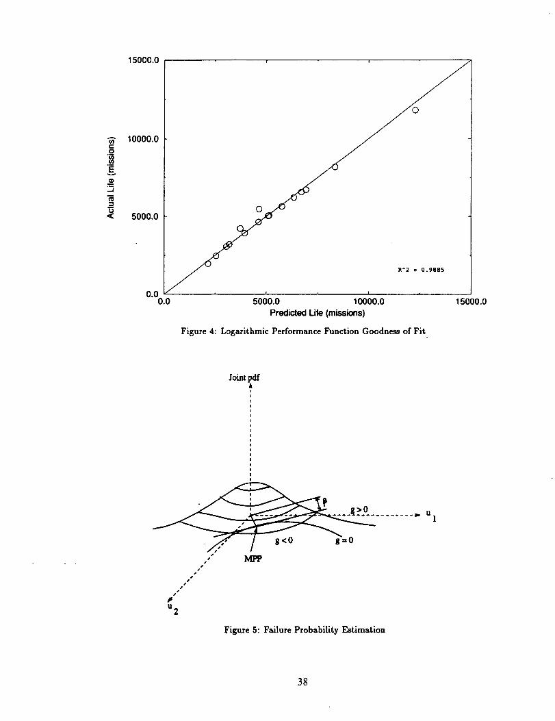
e
15000.0
10000.0
5000.0
0.00.0
i
R^2 = 0.9885
s i = I =
5000.0 10000.0 15000.0
Figure 4: Logarithmic Performance Function Goodness of Fit
Joint pdfA
s• MPP•J
p
u 2
Figure 5: Failure Probability Estimation
.._. U1
38
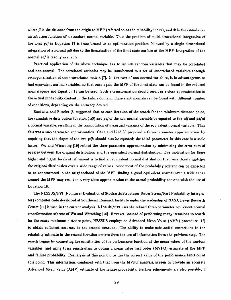
where _ is the distance from the origin to MPP (referred to as the reliability index), and _ is the cumulative
distribution function of a standard normal variable. Thus the problem of multi-dimensional integration of
the joint pdf in Equation 17 is transformed to an optimization problem followed by a single dimensional
integration of a normal pdfdue to the iinearization of the limit state surface at the MPP. Integration of the
normal pdf is readily available.
Practical application of the above technique has to include random variables that may be correlated
and non-normal. The correlated variables may be transformed to a set of uncorrelated variables through
orthogonalization of their covariance matrix [7]. In the case of non-normal variables, it is advantageous to
find equivalent normal variables, so that once again the MPP of the limit state can be found in the reduced
normal space and Equation 18 can be used. Such a transformation should result in a close approximation to
the actual probability content in the failure domain. Equivalent normals can be found with different number
of conditions, depending on the accuracy desired.
Rackwitz and Fiessler [8] suggested that at each iteration of the search for the minimum distance point,
the cumulative distribution function (cd]) and pdfof the non-normal variable be equated to the cdfand pdfof
a normal variable, resulting in the computation of mean and variance of the equivalent normal variable. Thus
this was a two-parameter approximation. Chert and Lind [9] proposed a three-parameter approximation, by
requiring that the slopes of the two pd.fs should also be equated; the third parameter in this case is a scale
factor. Wu and Wirsching [10] refined the three-parameter approximation by minimizing the error sum of
squares between the original distribution and the equivalent normal distribution. The motivation for these
higher and higher levels of refinement is to find an equivalent normal distribution that very closely matches
the original distribution over a wide range of values. Since most of the probability content can be expected
to be concentrated in the neighborhood of the MPP, finding a good equivalent normal over a wide range
around the MPP may result in a very close approximation to the actual probability content with the use of
Equation 18.
The NESSUS/FPI (Nonlinear Evaluation of Stochastic Structures Under Stress/Fast Probability Intergra-
tot) computer code developed at Southwest Research Institute under the leadership of NASA Lewis Research
Center [11] is used in the current analysis. NESSUS/FPI uses the refined three-parameter equivalent normal
transformation scheme of Wu and Wirsching [10]. However, instead of performing many iterations to search
for the exact minimum distance point, NESSUS employs an Advanced Mean Value (AMV) procedure [12]
to obtain sufficient accuracy in the second iteration. The ability to make substantial corrections to the
reliability estimate in the second iteration derives from the use of information from the previous step. The
search begins by computing the sensitivities of the performance function at the mean values of the random
variables, and using these sensitivities to obtain a mean value first order (MVFO) estimate of the MPP
and failure probability. Reanalysis at this point provides the correct value of the performance function at
this point. This information, combined with that from the MVFO analysis, is seen to provide an accurate
Advanced Mean Value (AMV) estimate of the failure probability. Further refinements are also possible, if
39
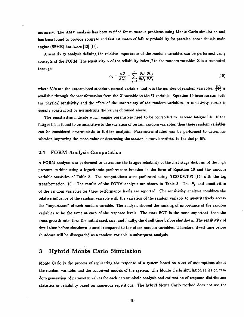
necessary. The AMV analysis has been verified for numerous problems using Monte Carlo simulation and
has been found to provide accurate and fast estimates of failure probability for practical space shuttle main
engine (SSME) hardware [13] [14].
A sensitivity analysis defining the relative importance of the random variables can be performed using
concepts of the FORM. The sensitivity a of the reliability index 8 to the random variables X is a computed
through
08 _ 08 au_ (19)- - j=
where//j's are the uncorrelated standard normal variable, and n is the number of random variables. _ is
available through the transformation from the X variable to the U variable. Equation 19 incorporates both
the physical sensitivity and the effect of the uncertainty of the random variables. A sensitivity vector is
usually constructed by normalizing the values obtained above.
The sensitivities indicate which engine parameters need to be controlled to increase fatigue life. If the
fatigue life is found to be insensitive to the variation of certain random variables, then these random variables
can be considered deterministic in further analysis. Parametric studies can be performed to determine
whether improving the mean value or decreasing the scatter is most beneficial to the design life.
2.1 FORM Analysis Computation
A FORM analysis was performed to determine the fatigue reliability of the first stage disk rim of the high
pressure turbine using a logarithmic performance function in the form of Equation 16 and the random
variable statistics of Table 2. The computations were performed using NESSUS/FPI [15] with the log
transformation [10]. The results of the FORM analysis are shown in Table 3. The PI and sensitivities
of the random variables for three performance levels are reported. The sensitivity analysis combines the
relative influence of the random variable with the variation of the random variable to quantitatively access
the "importance" of each random variable. The analysis showed the ranking of importance of the random
variables to be the same at each of the response levels. The start BOT is the most important, then the
crack growth rate, then the initial crack size, and finally, the dwell time before shutdown. The sensitivity of
dwell time before shutdown is small compared to the other random variables. Therefore, dwell time before
shutdown will be disregarded as a random variable in subsequent analysis.
3 Hybrid Monte Carlo Simulation
Monte Carlo is the process of replicating the response of a system based on a set of assumptions about
the random variables and the conceived models of the system. The Monte Carlo simulation relies on ran-
dom generation of parameter values for each deterministic analysis and estimation of response distribution
statistics or reliability based on numerous repetitions. The hybrid Monte Carlo method does not use the
4O
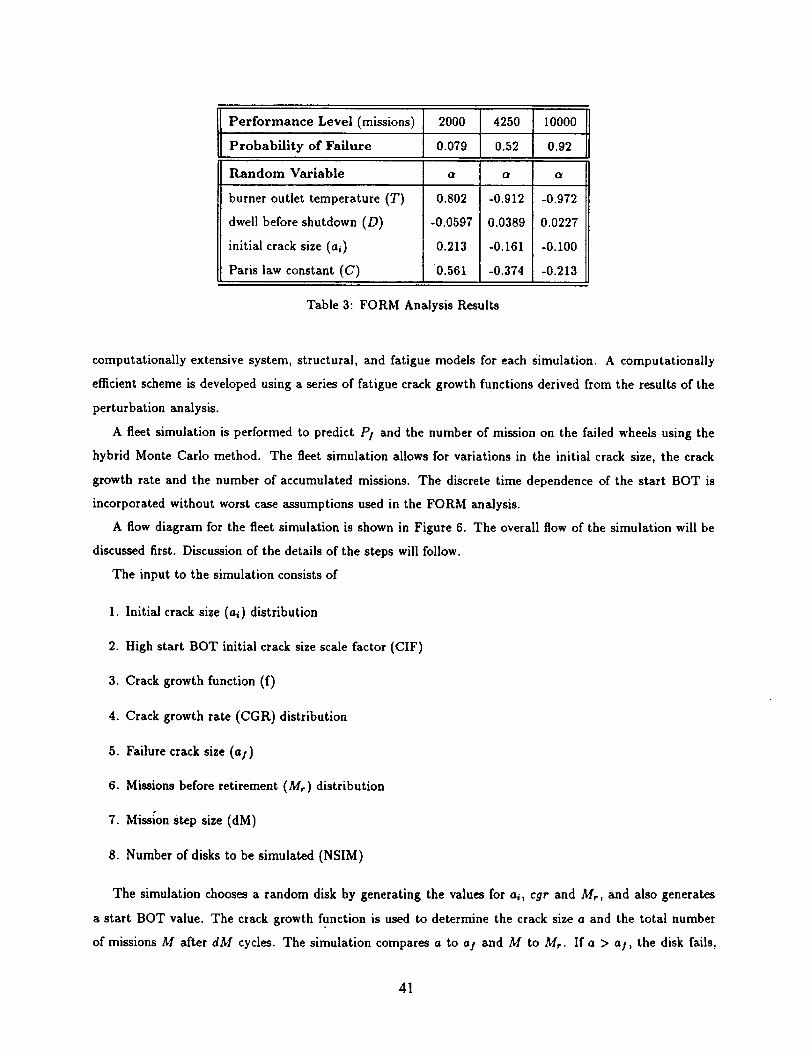
Performance Level (missions) 2000
Probability of Failure 0.079
Random Variable a
burner outlet temperature (T)
dwell before shutdown (D)
initial crack size (ai)
Paris law constant (C)
0.802
-0.0597
0.213
0.561
4250
0.52
-0.912
0.0389
-0.161
-0.374
Table 3: FORM Analysis Results
10000
0.92
a
-0.972
0.0227
-0.100
-0.213
computationally extensive system, structural, and fatigue models for each Simulation. A computationally
efficient scheme is developed using a series of fatigue crack growth functions derived from the results of the
perturbation analysis.
A fleet simulation is performed to predict PI and the number of mission on the failed wheels using the
hybrid Monte Carlo method. The fleet simulation allows for variations in the initial crack size, the crack
growth rate and the number of accumulated missions. The discrete time dependence of the start BOT is
incorporated without worst case assumptions used in the FORM analysis.
A flow diagram for the fleet simulation is shown in Figure 6. The overall flow of the simulation will be
discussed first. Discussion of the details of the steps will follow.
The input to the simulation consists of
1. Initial crack size (ai) distribution
2. High start BOT initial crack size scale factor (CIF)
3. Crack growth function (f)
4. Crack growth rate (CGR) distribution
5. Failure crack size (a I)
6. Missions before retirement (M,) distribution
7. Mission Step size (dM)
8. Number of disks to be simulated (NSIM)
The simulation chooses a random disk by generating the values for ai, cgr and M,, and also generates
a start BOT value. The crack growth function is used to determine the crack size a and the total number
of missions M after dM cycles. The simulation compares a to a I and M to M,. If a > a/, the disk fails,
41
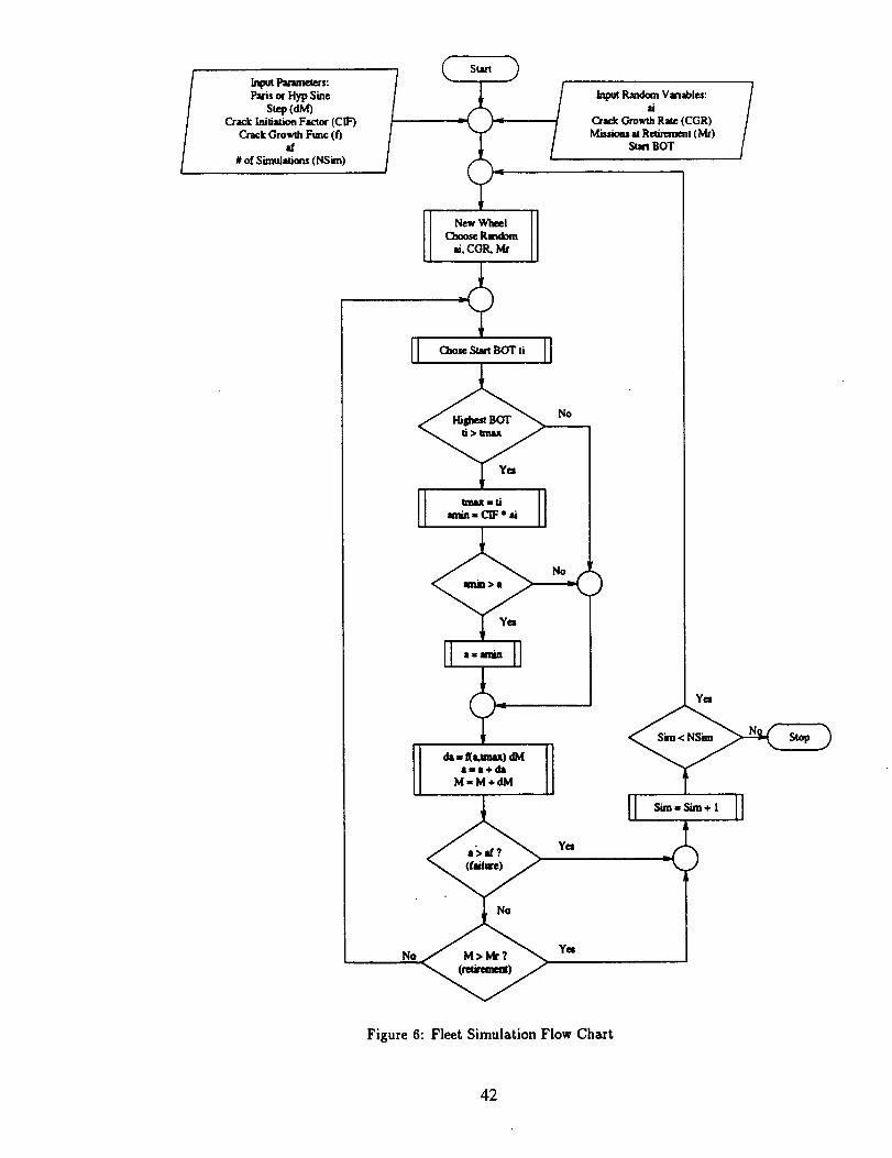
Inttm_p,anunem's"Pros o+H,/_Sine
StW (dld)O_J. _,iti_on Factor+elF)
Crack Growth Free (t')if
# of Simel_om (NS_)
No
No M>Mr?
Figure 6: FleetSimulation Flow Chazt
42
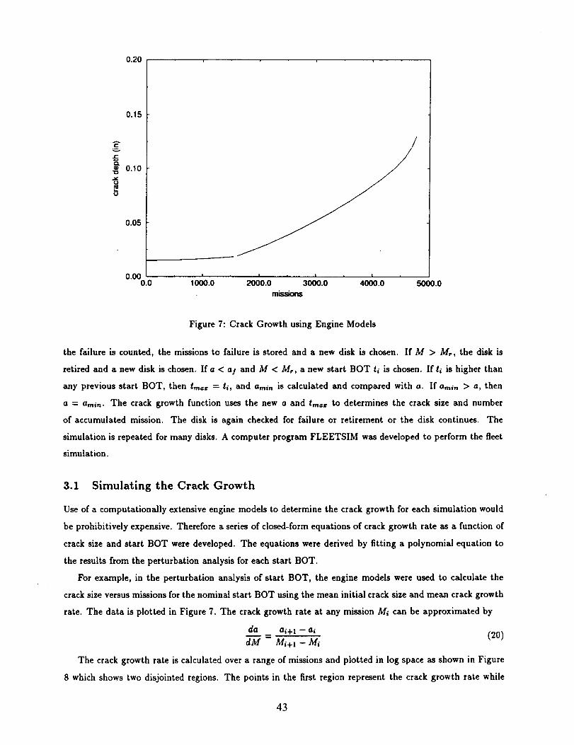
0.20 , ,
0.15
O.® 0.10"0
U
0.05
, !
o.OOo.0 10o0.oI , I I
2000.0 3000.0 4000.0 5000.0
missions
Figure 7: Crack Growth using Engine Models
the failure is counted, the missions to failure is stored and a new disk is chosen, If M > Mr, the disk is
retired and a new disk is chosen. If a < a! and M < Mr, a new start BOT ti is chosen. If tl is higher than
any previous start BOT, then t,,_== = ti, and am_. is calculated and compared with a. If amin > a, then
a = a,.i.. The crack growth function uses the new a and trnaz to determines the crack size and number
of accumulated mission. The disk is again checked for failure or retirement or the disk continues. The
simulation is repeated for many disks. A computer program FLEETSIM was developed to perform the fleet
simulation.
3.1 Simulating the Crack Growth
Use of a computationally extensive engine models to determine the crack growth for each simulation would
be prohibitively expensive. Therefore a series of closed-form equations of crack growth rate as a function of
crack size and start BOT were developed. The equations were derived by fitting a polynomial equation to
the results from the perturbation analysis for each start BOT.
For example, in the perturbation analysis of start BOT, the engine models were used to calculate the
crack size versus missions for the nominal start BOT using the mean initial crack size and mean crack growth
rate. The data is plotted in Figure 7. The crack growth rate at any mission Mi can be approximated by
da _ ai+l - ai (20)dM Mi+z - Mi
The crack growth rate is calculated over a range of missions and plotted in log space as shown in Figure
8 which shows two disjointed regions. The points in the first region represent the crack growth rate while
43
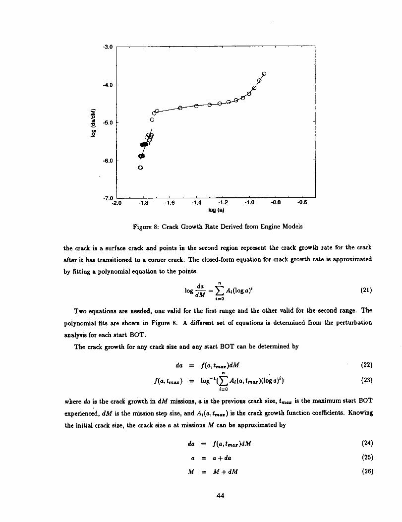
-3.0
_g
-4.0
-5.0
-6.0
O
O
! , i , i t
"7"02.0 ' "1'.8 ' -1.6 "1'.4 "1'.2 -1'.0 _.8 "0.6
tOg(a)
Figure 8: Crack Growth Rate Derived from Engine Models
the crack is a surface crack and points in the second region represent the crack growth rate for the crack
after it has transitioned to a corner crack. The closed-form equation for crack growth rate is approximated
by fitting a polynomial equation to the points.
dalog = A,(log.)' (2t)
i=O
Two equations are needed, one valid for the first range and the other valid for the second range. The
polynomial fits are shown in Figure 8. A different set of equations is determined from the perturbation
analysis for each start BOT.
The crack growth for any crack size and any start BOT can be determined by
da = f(a,t,n,r)dM (22)rl
f(a, tra,,) = log-l(E Ai(a,tn_az)(loga)i) (23)i=0
where da is the cracl/growth in dM missions, a is the previous crack size, tra_ is the maximum start BOT
experienced, dM is the mission step size, and Ai(a, tmaz) is the crack growth function coefficients. Knowing
the initial crack size, the crack size a at missions M can be approximated by
da = f(a, tma::)dM (24)
a = a + da (25)
M = M + dM (26)
44
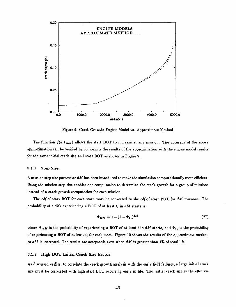
Ae-
J:
O.
J¢
¢J
0.20
0.15
0.10
0.05
i
ENGINE MODELS --
APPROXIMATE METHOD ....
fi
i
I t
t
I I
i I , I i | I I
0"000.0 1000.0 2000.0 3000.0 4000.0 5000.0
missions
Figure 9: Crack Growth: Engine Model vs. Approximate Method
The function f(a, t,,_,=)allowsthe startBOT to increaseat any mission. The accuracy of the above
approximation can be verifiedby comparing the resultsof the approximation with the engine model results
forthe same initialcrack sizeand startBOT asshown in Figure 9.
3.1.1 Step Size
A mission step size parameter dM has been introduced to make the simulation computationally more efficient.
Using the mission step size enables one computation to determine the crack growth for a group of missions
instead of a crack growth computation for each mission.
The cdf of start BOT for each start must be converted to the cdf of start BOT for dM missions. The
probability of a disk experiencing a BOT of at least tl in dM starts is
_raM = I - (1 - _tl) aM (27)
where _I¢ld M is the probability of experiencing a BOT of at least t in dM starts, and _tl is the probability
of experiencing a BOT of at least ti for each start. Figure 10 shows the results of the approximate method
as dM is increased. The results are acceptable even when dM is greater than 1% of total life.
3.1.2 High BOT Initial Crack Size Factor
As discussed earlier, to correlate the crack growth analysis with the early field failures, a large initial crack
size must be correlated with high start BOT occurring early in life. The initial crack size is the effective
45
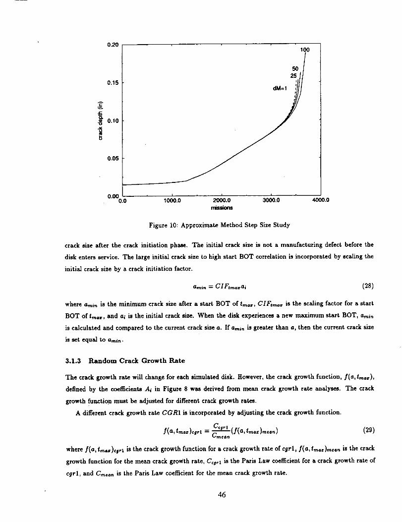
n
"o
g
0.20
0.15
0.10
0-05
100
25
dM=1 i
I . I I ,
0"_0.0 1_0.0 2000.0 3_0.0 4000.0
missions
Figure 10: Approximate Method Step Size Study
crack size after the crack initiation phase. The initial crack size is not a manufacturing defect before the
disk enters service. The large initial crack size to high start BOT correlation is incorporated by scaling the
initial crack size by a crack initiation factor.
a,,i, = C I Ftm==a, (28)
where a,,.,_ is the minimum crack size after a start BOT of t,.==, CIFt._== is the scaling factor for a start
BOT of t._==, and ai is the initial crack size. When the disk experiences a new maximum start BOT, a,_i.
is calculated and compared to the current crack size a. If a... is greater than a, then the current crack size
is set equal to a,_i,,.
3.1.3 Random Crack Growth Rate
The crack growth rate will change for each simulated disk. However, the crack growth function, f(a, tin,=),
defined by the coefficients Ai in Figure 8 was derived from mean crack growth rate analyses. The crack
growth function must be adjusted for different crack growth rates.
A different crack growth rate CGR1 is incorporated by adjusting the crack growth function.
f(=. = t.=o.)m...) (29)
where f(a, tm°=)¢s_l is the crack growth function for a crack growth rate of cgrl, f(a,tma=)mean is the crack
growth function for the mean crack growth rate, C¢g.1 is the Paris Law coefficient for a crack growth rate of
cgrl, and Cm.o. is the Paris Law coefficient for the mean crack growth rate.
46
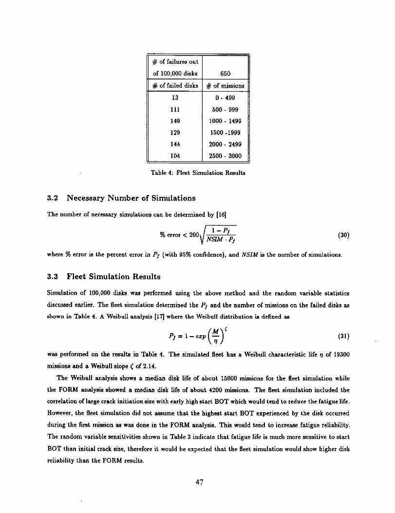
# of failures out
of 100,000 disks 650
# of failed disks # of missions
13
111
149
129
144
104
0- 499
500- 999
1000- 1499
1500-1999
2000- 2499
2500- 3000
Table 4: Fleet Simulation Results
3.2 Necessary Number of Simulations
The number of necessary simulations can be determined by [16]
- PI% error< 200 MS7M •P!(30)
where % error is the percent error in P! (with 95% confidence), and NSIM is the number of simulations.
3.3 Fleet Simulation Results
Simulation of 100,000 disks was performed using the above method and the random variable statistics
discussed earlier. The fleet simulation determined the P! and the number of missions on the failed disks as
shown in Table 4. A Weibull analysis [17] where the Weibull distribution is defined as
PI= I- (31)
The simulated fleet has a Weibull characteristic life _ of 19300was performed on the results in Table 4.
missions and a Weibull slope _ of 2.14.
The Weibull analysis shows a median disk life of about 15000 missions for the fleet simulation while
the FORM analysis showed a median disk life of about 4200 missions. The fleet simulation included the
correlation of large crack initiation size with early high start BOT which would tend to reduce the fatigue life.
However, the fleet simulation did not assume that the highest start BOT experienced by the disk occurred
during the first mission as was done in the FORM analysis. This would tend to increase fatigue reliability.
The random variable sensitivities shown in Table 3 indicate that fatigue life is much more sensitive to start
BOT than initial crack size, therefore it would be expected that the fleet simulation would show higher disk
reliability than the FORM results.
47
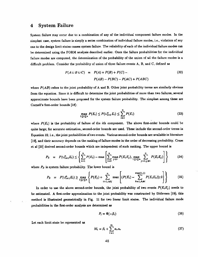
4 System Failure
System failure may occur due to a combination of any of the individual component failure modes. In the
simplest case, system failure is simply a series combination of individual failure modes, i.e., violation of any
one to the design limit states causes system failure. The reliability of each of the individual failure modes can
be determined using the FORM analysis described earlier. Once the failure probabilities for the individual
failure modes are computed, the determination of the probability of the union of all the failure modes is a
difficult problem. Consider the probability of union of three failure events A, B, and C, defined as
P(AUBtgC) = P(A)+ P(B)+ P(C)- (32)
P(AB) - P(BC) - P(AC) + P(ABC)
where P(AB) refers to the joint probability of A and B. Other joint probability terms are similarly obvious
from the equation. Since it is difficult to determine the joint probabilities of more than two failures, several
approximate bounds have been proposed for the system failure probability. The simplest among these are
Cornell's first-order bounds [18]:
max P(Ei) < P(U_=IEi) < _P(Ei) (33)l <i<_n -- i-_l
where P(E_) is the probability of failure of the ith component. The above first-order bounds could be
quite large; for accurate estimation, second-order bounds are used. These include the second-order terms in
Equation 32, i.e., the joint probabilities of two events. Various second-order bounds are available in literature
[19], and their accuracy depends on the ranking of failure modes in the order of decreasing probability. Cruse
et al [20] derived second-order bounds which are independent of such ranking. The upper bound is
Ps = P(tg_=lEi) _< P(E_) - max maxP(EiEj), max _ P(EiE_)i---1 j<i l<i_nj__l,j$i
where Ps is system failure probability. The lower bound is
Ps = P(U_'=IEi)> max P(Ej)+ __, max (P(Ei)- P(EIEk));O-- -- Igjgn
-- L _=l,i_j kfl,k#i
(34)
(35)
In order to use the above second-order bounds, the joint probability of two events P(EiE_) needs to
be estimated. A first-order approximation to the joint probability was constructed by Ditlevsen [19]; this
method is illustrated geometrically in Fig. 11 for two linear limit states. The individual failure mode
probabilities in the first-order analysis are determined as
P, = ¢(-_,) (30)
Let each limit state be represented as
Mi - _ + E a,u, (37)r----|
48
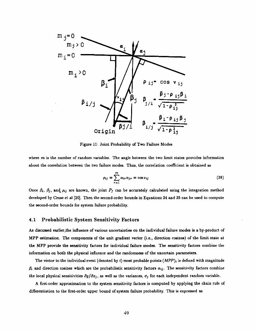
mj=O
mj>O
rni=O
mi>O /
Figure lh Joint Probability of Two Failure Modes
where m is the number of random variables.
about the correlation between the two failure modes. Thus, the correlation coefficient is obtained as
p_j= _,,_,ai,= co, _,_ (38)rffil
Once _i, _j, and Pij are known, the joint P! can be accurately calculated using the integration method
developed by Cruse et al [20]. Then the second-order bounds in Equations 34 and 35 can be used to compute
the second-order bounds for system failure probability.
The angle between the two limit states provides information
4.1 Probabilistic System Sensitivity Factors
As discussed earlier,the influence of various uncertainties on the individual failure modes is a by-product of
MPP estimation. The components of the unit gradient vector (i.e., direction cosines) of the limit state at
the MPP provide the sensitivity factors for individual failure modes. The sensitivity factors combine the
information on both the physical influence and the randomness of the uncertain parameters.
The vector to the individual event (denoted by i) most probable points (MPP)i is defined with magnitude
_/i and direction cosines which are the probabilistic sensitivity factors aij. The sensitivity factors combine
the local physical sensitivities ag/azj, as well as the variances, _j for each independent random variable.
A first-order approximation to the system sensitivity factors is computed by applying the chain rule of
differentiation to the first-order upper bound of system failure probability. This is expressed as
49
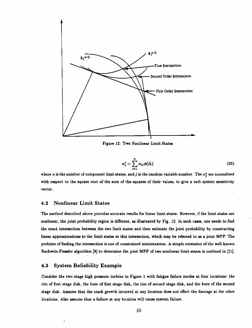
j,,0_L_True Intersection
Figure 12: Two Nonlinear Limit States
I1
a_ = _ aij_(/_i) (39)ill
Jwhere n is the number of component limit states, and j is the random variable number. The aj are normalized
with respect to the square root of the sum of the squares of their values, to give a unft system sensitivity
vector.
4.2 Nonlinear Limit States
The method described above provides accurate results for linear limit states. However, if the limit states are
nonlinear, the joint probability region is different, as illustrated by Fig. 12. In such cases, one needs to find
the exact intersection between the two limit states and then estimate the joint probability by constructing
linear approximations to the limit states at this intersection, which may be referred to as a joint MPP. The
problem of finding the intersection is one of constrained minimization. A simple extension of the well-known
Rackwitz-Fiessler algorithm [8] to determine the joint MPP of two nonlinear limit states is outlined in [21].
4.3 System Reliability Example
Consider the two stage high pressure turbine in Figure 1 with fatigue failure modes at four locations: the
rim of first stage disk, the bore of first stage disk, the rim of second stage disk, and the bore of the second
stage disk. Assume that the crack growth incurred at any location does not effect the damage at the other
locations. Also assume that a failure at any location will cause system failure.
50
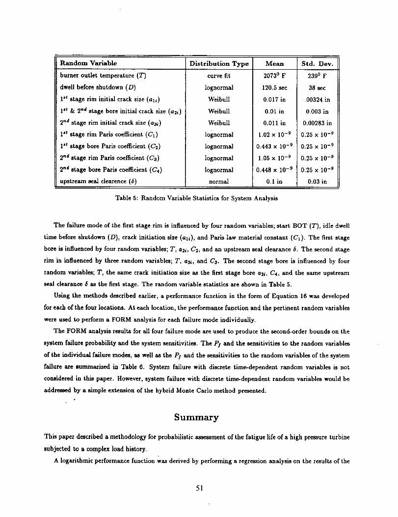
Random Variable Distribution Type Mean Std. Dev.
burner outlet temperature (T)
dwell before shutdown (D)
1 't stage rim initial crack size (al_)
1't & 2'_d stage bore initial crack size (a2i)
curve fit
lognormal
Weibull
Weibull
20730 F
120.5sec
0.017 in
0.01 in
2_a stage rim initial crack size (aa_)
1 't stage rim Paris coefficient (C1)
1't stage bore Paris coefficient (C2)
2nd stage rim Paris coefficient (C3)
2nd stage bore Paris coefficient (C4)
upstream seal clearence (6)
Weibull
lognormal
lognormal
lognormal
lognormal
normal
0.011 in
1.02 x 10 -9
0.443 x 10 -9
1.05 x 10 -9
0.448 x 10 -9
0.1 in
2390 F
38 sec
.00324 in
0.003 in
0.00283 in
0.25 x 10 -9
0.25 x 10⁻⁹
0.25 x 10 -9
0.25 x 10 -9
0.03 in
Table 5: Random VariableStatisticsforSystem Analysis
The failure mode of the first stage rim is influenced by four random variables; start BOT (T), idle dwell
time before shutdown (D), crack initiation size (all), and Paris law material constant (C1). The first stage
bore is influenced by four random variables; T, a21, C2, and an upstream seal clearance 6. The second stage
rim in influenced by three random variables; T, asl, and (73. The second stage bore is influenced by four
random variables; T, the same crack initiation size as the first stage bore a_i, C4, and the same upstream
seal clearance 5 as the first stage. The random variable statistics are shown in Table 5.
Using the methods described earlier, a performance function in the form of Equation 16 was developed
for each of the four locations. At each location, the performance function and the pertinent random variables
were used to perform a FORM analysis for each failure mode individually.
The FORM analysis results for all four failure mode are used to produce the second-order bounds on the
system failure probability and the system sensitivities. The P! and the sensitivities to the random variables
of the individual failure modes, as well as the P! and the sensitivities to the random variables of the system
failure are summarized in Table 6. System failure with discrete time-dependent random variables is not
considered in this paper. However, system failure with discrete time-dependent random variables would be
addressed by a simple extension of the hybrid Monte Carlo method presented.
Summary
This paper described a methodology for probabilistic assessment of the fatigue life of a high pressure turbine
subjected to a complex load history.
A logarithmic performance function was derived by performing a regression analysis on the results of the
51
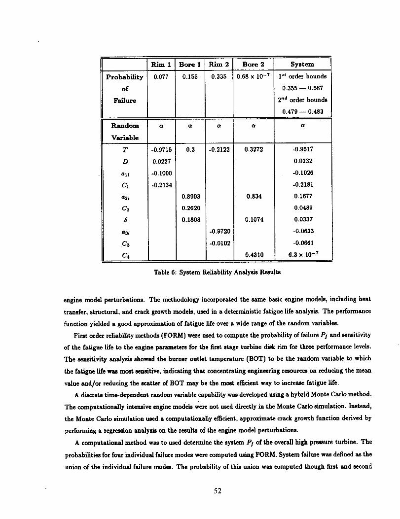
Probability
of
Failure
Random
Variable
T
D
ali
Cz
a2_
C2
6
a3/
c3
c_
-0.9715
Bore 1
0.155
0.3
Rim2
0.335
-0.2122
Bore 2
0.68 x 10 -7
0.3272
System
1"t order bounds
0.355m0.567
2"d order bounds
0.479m0.483
ot
-0.9517
0.0227
-0.1000
-0.2134
0.8993
0.2620
0.1808
-0.9720
-0.0102
0.834
0.1074
0.4310
0.0232
-0.I026
-0.2181
0.1677
0.0489
0.0337
-0.0633
-0.0661
6.3 x 10⁻⁷
Table 6: System Reliability Analysis Results
engine model perturbations. The methodology incorporated the same basic engine models, including heat
transfer, structural, and crack growth models, used in a deterministic fatigue life analysis. The performance
function yielded a good approximation of fatigue life over a wide range of the random variables.
First order reliability methods (FORM) were used to compute the probability of failure P! and sensitivity
of the fatigue life to the engine parameters for the first stage turbine disk rim for three performance levels.
The sensitivity analysis showed the burner outlet temperature (BOT) to be the random variable to which
the fatigue life was most sensitive, indicating that concentrating engineering resources on reducing the mean
value and/or reducing the scatter of BOT may be the most efficient way to increase fatigue life.
A discrete time-dependent random variable capability was developed using a hybrid Monte Carlo method.
The computationally intensive engine models Were not used directly in the Monte Carlo simulation. Instead,
the Monte Carlo simulation used. a computationally efficient, approximate crack growth function derived by
performing a regression analysis on the results of the engine model perturbations.
A computational method was to used determine the system P! of the overall high pressure turbine. The
probabilities for four individual failure modes were computed using FORM. System failure was defined as the
union of the individual failure modes. The probability of this union was computed though first and second
52

order bounds. Tile method also provided sensivity information about the effect of each random variable on
the individual failure probabilities as well a.s the system failure probability. The burner outlet temperature
(BOT) was found to be the random variable to which the fatigue life of the overall turbine was most sensitive.
Acknowledgments - This work was partially supported by NASA contract NAS3-24389, Lewis Research
Center, Dr. C. C. Chamis, Program Manager; NASA GSRP Project NGT-51053, Lewis Research Center,
Dr. C. C. Chamis, Technical Advisor; and Allison Gas Turbine contract H135571, Dr. ,1. E. Pope, Project
Engineer.
53
References
[1] Cruse, T.A., Mahadevan, S., Tryon, R.G., "Fatigue Reliability of Gas Turbine Engines, Part I - Method-
ologies Developed", Engineering Fracture Mechanics, under review.
I2] Socie, D.F. and Kuranth, P., "Cycle Counting for Variable Amplitude Crack Growth", Fracture Me-
chanics: Fourteenth Symposium, Vol 2, ASTM STP 791, 1983, pp II-19 - II-32.
[3] Asquith G. and Pickard A.C.,"Fatigue Testing of Gas Turbine Components", High Temperature
Technology, Vol 6, No 3, August 1988, pp 131-143.
[4] Yang, J.N., Salivar, G.C., Annis, C.G., Statistics of Crack Growth in Engine Materials - Vol-
ume 1: Constant Amplitude Fatigue Crack Growth at Elevated Temperatures, AFWAL-
TR-82-4040.
[5] Provan, J.W., Probabilistic Fracture Mechanics and Reliability, Martinus Nijhoff, Dordrecht,
The Netherlands, 1987.
[6] Hasofer, A.M. and Lind, N.C., "Exact and Invariant Second Moment Code Formst", Journal of the
Engineering Mechanics Division, ASCE, Vol 100, No.EM1, pp. 111-121, 1985
[7] Ang, A. H.-S. and Tang, W.H., Probability Concepts in Engineering Planning and Design,
Vol 2, John Wiley and Sons, New York, 1975.
[8] Rackwitz, R. and Fiessler, B, "Structural Reliability Under Combined Random Load Sequences", Com-
puters and Structures. Vol. 9, No. 5, pp. 484-494, 1978.
[9] Chen, X., and Lind, N.C., "Fast Probability Integration by Three-Parameter Normal Tail Approxima-
tion", Structural Safety, Vol. 1, pp. 269-276, 1983.
[10] Wu, Y.T., and Wirsching, P.H., "New algorithm for structural reliability estimation", Journal of
Engineering Mechanics, ASCE, Vol. 113, No. 9, pp. 1319-1336, 1987.
[11] Cruse, T.A., Chamis, C.C., and Millwater, H.R., "An Overview of the NASA(LeRC)-SwKI Prob_-
bilistic Structural Analysis (PSAM) Program", Proceedings, 5th International Conference on
Structural Safety and Reliability (ICOSSAR), San Francisco, California, pp. 2267-2274, 1989.
[12] Wu, Y.T., MiUwater, H.R., and Cruse, T.A., "An Advanced Probabilistic Structural Analysis Method
for Implicit Performance Functions", AIAA Journal, Vol. 28, No. 9, pp. 1663-1669, 1990.
[13] Cruse, T.A., Burnside, O.H., Wu, Y.-T., Polch, E.Z., and Dias, J.B., "Probabilistic Structural Analy-
sis Methods for Select Space Propulsion System Structural Components (PSAM) =, Computers and
Structures1 Vol. 29(5), pp. 891-901, 1988.
54
[14] Rajagopal, K.R., Debchaudhury, A., and Newell, J.F., "Verification of NESSUS Code on Space Propul-
sion Components", Proceedings, 5th International Conference on Structural Safety and Re-
liability, ICOSSAR '89, San Francisco, California, pp. 2299-2306, 1989.
[15] "NESSUS Reference Manual," Version 1.0, July 1991, Southwest Research Institute, TX.
[16] Ang, A. H.-S. and Tang, W.H., Probability Concepts in Engineering Planning and Design,
Vol 2, John Wiley and Sons, New York, 1975.
[17] Abernethy, R.B., Breneman, J.E., Medlin, C.H., Reinman, G.L., Weibull Analysis Handbook,
AFWAL-TR-83.2079, November 1983.
[18] Cornell, C.A., "Bounds on the Reliability of Structural Systems", Journal of the Structural Divi-
sion, ASCE, Vol. 93, No. ST1, pp. 171-200, 1967.
[19] Ditlevsen, O., "Narrow Reliability Bounds for Structural Systems", Journal of Structural Mechan-
ics, Vol. 3, 453-472, 1979.
[20] Cruse, T.A., Huang, Q., Mehta, S., and Mahadevan, S., "System Reliability and Risk Assessment", Pro-
ceedlngs of the 33rd AIAA/ASME/ASCE/AHS/ASC Conference on Structures, Struc-
tural Dynamics and Materials, Dallas, Texas, pp.424-431, 1992.
[21] Mahadevan, S., and Cruse, T.A., "An Advanced First-Order Method for System Reliability," Proceed-
ings of the ASCE Joint Specialty Conference on Probabilistic Mechanics and Structural
and Geotechnical Reliability, Denver, Colorado, pp. 487-490, 1992.
55
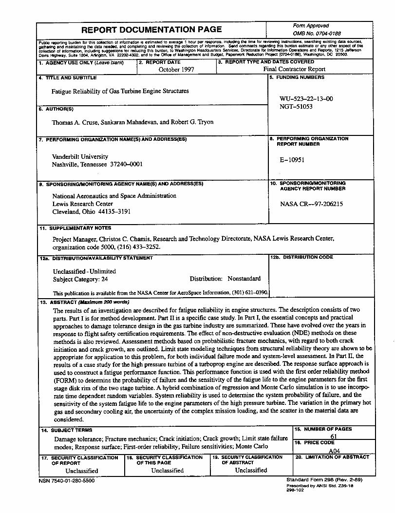
REPORT DOCUMENTATION PAGE FormApprovedOMB No. 0704-0188
Publicreportingburdenforthiscollectionofinformationisestimatedtoaverage1hourperresponse,includingthetimeforreviewinginstructions,searchingexistingdatasources,gatheringandmaintainingthedataneeded,andcompletingandreviewingthe.collectionofinformatio_Sendcommlmtsr.ege.rd.mgthisburdenestimateoranyotheraSl:_..ofthiscollectionofinformation,includingsuggestionsforreducingthisburden,towasningtonHeadcluarters::;ervices,u=mctoratemr inTormat_onuperaUonsandReports,12]_JenereonDavisHighway,Suite1204,Arlington,VA 22202-4302,andtotheOfficeofManagementandBudget,Paperwod(ReductionProj_'t(0704-0188},Washington,DC 20503.
1. AGENCYUSEONLY (Leaveblank) 2. REPORTDATEOctober 1997
4. TITLEANDSUBTITLE
Fatigue Reliability of Gas Turbine Engine Structures
6. AUTHOR(S)
Thomas A. Cruse, Sankaran Mahadevan, and Robert G. Tryon
7. PERFORMINGORGANIZATIONNAME(S)AND ADDRESS(ES)
Vanderbilt UniversityNashville, Tennessee 37240--0001
9. SPONSORING/MONITORINGAGENCYNAME(S)ANDADDRESS(ES)
National Aeronautics and Space AdministrationLewis Research Center
Cleveland, Ohio 44135-3191
3. REPORTTYPEAND DAi_ COVERED
Final Contractor Report5. FUNDINGNUMBERS
WU-523-22-13-00
NGT-51053
8. PERFORMINGORGANIZATIONREPORTNUMBER
E-10951
10. SPONSORING/MONITORINGAGENCYREPORTNUMBER
NASA CR--97-206215
11. SUPPLEMENTARYNOTES
Project Manager, Christos C. Chamis, Research and Technology Directorate, NASA Lewis Research Center,
organization code 5000, (216) 433-3252.
12a. DISTRIBUTION/AVAILABILITYSTATEMENT
Unclassified - Unlimited
Subject Category: 24 Distribution: Nonstandard
This publication is available from the NASA Center for AeroSpace Information. (301) 621--0390.
12b. DISTRIBUTIONCODE
13. ABSTRACT(Maximum200 words)
The results of an investigation are described for fatigue reliability in engine structures. The description consists of two
parts. Part I is for method development. Part 1"Iis a specific case study. In Part I, the essential concepts and practical
approaches to damage tolerance design in the gas turbine industry are summarized. These have evolved over the years in
response to flight safety certification requirements. The effect of non-destructive evaluation (/fiDE) methods on thesemethods is also reviewed. Assessment methods based on probabilistic fracture mechanics, with regard to both crack
initiation and crack growth, are oudined. Limit state modeling techniques from structural reliability theory are shown to be
appropriate for application to this problem, for both individual failure mode and system-level assessment. In Part II, theresults of a case study for the high pressure turbine of a turboprop engine are described. The response surface approach is
used to construct a fatigue performance function. This performance function is used with the first order reliability method
(FORM) to determine the probability of failure and the sensitivity of the fatigue life to the engine parameters for the first
stage disk rim of the two stage turbine. A hybrid combination of regression and Monte Carlo simulation is to use incorpo-
rate time dependent random variables. System reliability is used to determine the system probability of failure, and the
sensitivity of the system fatigue life to the engine parameters of the high pressure turbine. The variation in the primary hot
gas and secondary cooling air, the uncertainty of the complex mission loading, and the scatter in the material data areconsidered.
14. SUBJECT TERMS
Damage tolerance; Fracture mechanics; Crack initiation; Crack growth; Limit state failure
modes; Response surface; First-order reliability; Failure sensitivities; Monte Carlo
17. SECURITYCLASSIFICATIONOF REPORT
Unclassified
18. SECURITYCLASSIFICATIONOFTHIS PAGE
Unclassified
NSN 7540-01-280-5500
19. SECURITYCLASSIFICATIONOFABSTRACT
Unclassified
15. NUMBEROF PAGES
6116. PRICECODE
A0420. LIMITATIONOF ABSTRACT
Standard Form298 (Rev. 2-89)PrescribedbyANSIStd.Z39-18298-102