fatigue assessment of offshore structures - … · guide for the fatigue assessment of offshore...
TRANSCRIPT
G u i d e f o r t h e F a t i g u e A s s e s s m e n t o f O f f s h o r e S t r u c t u r e s
GUIDE FOR
FATIGUE ASSESSMENT OF OFFSHORE STRUCTURES
APRIL 2003 (Updated March 2018 – see next page)
American Bureau of Shipping Incorporated by Act of Legislature of the State of New York 1862
2003 American Bureau of Shipping. All rights reserved. ABS Plaza 16855 Northchase Drive Houston, TX 77060 USA

Updates
March 2018 consolidation includes: • February 2014 version plus Corrigenda/Editorials
February 2014 consolidation includes: • November 2010 version plus Corrigenda/Editorials
November 2010 consolidation includes: • April 2003 version plus Corrigenda/Editorials

F o r e w o r d
Foreword The main purpose of this Guide is to supplement the Rules and the other design and analysis criteria that ABS has issued for the Classification of some types of offshore structures. The specific Rules and other Classification criteria that are being supplemented by this Guide include the latest versions of the following documents:
• Rules for Building and Classing Offshore Installations
• Rules for Building and Classing Mobile Offshore Drilling Units
• Rules for Building and Classing Single Point Moorings
• Rules for Building and Classing Floating Production Installations
(However, the fatigue assessment of Ship-Type Floating Installations should be treated in accordance with the FPI Rules, and not this Guide)
While some of the criteria contained herein may be applicable to ship structure, it is not intended that this Guide be used in the Classification of a ship.
ABS welcomes comments and suggestions for improvement of this Guide. Comments or suggestions can be sent electronically to [email protected].
ABS GUIDE FOR THE FATIGUE ASSESSMENT OF OFFSHORE STRUCTURES . 2003 iii

T a b l e o f C o n t e n t s
GUIDE FOR
FATIGUE ASSESSMENT OF OFFSHORE STURCTURES CONTENTS SECTION 1 Introduction ............................................................................................ 1
1 Terminology and Basic Approaches Used in Fatigue Assessment .... 1 1.1 General ............................................................................................ 1 1.3 S-N Approach .................................................................................. 2 1.5 Fracture Mechanics ......................................................................... 2 1.7 Structural Detail Types .................................................................... 2
3 Damage Accumulation Rule and Fatigue Safety Checks ................... 2 3.1 General ............................................................................................ 2 3.3 Definitions ........................................................................................ 3 3.5 Fatigue Safety Check ...................................................................... 3
5 Existing Structures .............................................................................. 3 7 Summary ............................................................................................. 3 FIGURE 1 Schematic of Fatigue Assessment Process
(For each location or structural detail) ...................................... 4 SECTION 2 Fatigue Strength Based on S-N Curves ................................................ 5
1 Introduction ......................................................................................... 5 1.1 General ............................................................................................ 5 1.3 Defining Parameters ........................................................................ 5 1.5 Tolerances and Alignments ............................................................. 5
3 Nominal Stress Method ....................................................................... 5 3.1 ‘Reference’ Stress and Stress Concentration Factor ....................... 5
5 Hot Spot Stress Method ...................................................................... 7 5.1 Non-Tubular Joints .......................................................................... 7 5.3 Tubular Joints .................................................................................. 7 5.5 Stress Definitions and Related Approaches .................................... 8 5.7 Finite Element Analysis to Obtain Hot Spot Stress .......................... 9 5.9 FEA Data Interpretation – Stress Extrapolation Procedure and
S-N Curves ...................................................................................... 9 FIGURE 1 Two-Segment S-N Curve .......................................................... 7 FIGURE 2 Stress Gradients (Actual & Idealized) Near a Weld .................. 8
iv ABS GUIDE FOR THE FATIGUE ASSESSMENT OF OFFSHORE STRUCTURES . 2003

SECTION 3 S-N Curves ............................................................................................ 11 1 Introduction ....................................................................................... 11 3 S-N Curves and Adjustments for Non-Tubular Details
(Specification of the Nominal Fatigue Strength Criteria) .................. 11 3.1 ABS Offshore S-N Curves ............................................................. 11 3.3 AWS S-N Curves for Non-Tubular Details ..................................... 12
5 S-N Curves for Tubular Joints .......................................................... 16 5.1 ABS Offshore S-N Curves ............................................................. 16 5.3 API S-N Curves ............................................................................. 17 5.5 Parametric Equations for Stress Concentration Factors ................ 18
7 Cast Steel Components .................................................................... 19 TABLE 1 Parameters for ABS-(A) Offshore S-N Curves for Non-
Tubular Details in Air ............................................................... 13 TABLE 2 Parameters for ABS-(CP) Offshore S-N Curves for Non-
Tubular Details in Seawater with Cathodic Protection ............ 14 TABLE 3 Parameters for ABS-(FC) Offshore S-N Curves for Non-
Tubular Details in Seawater for Free Corrosion ..................... 15 TABLE 4 Parameters for Class ‘T’ ABS Offshore S-N Curves ............... 17 TABLE 5 Parameters for API S-N Curves for Tubular Joints ................. 18 TABLE 6 Parameters for ABS Offshore S-N Curve for Cast Steel
Joints (in-air) ........................................................................... 19 FIGURE 1 ABS-(A) Offshore S-N Curves for Non-Tubular Details in
Air ............................................................................................ 13 FIGURE 2 ABS-(CP) Offshore S-N Curves for Non-Tubular Details in
Seawater with Cathodic Protection ......................................... 14 FIGURE 3 ABS-(FC) Offshore S-N Curves for Non-Tubular Details in
Seawater for Free Corrosion ................................................... 15 FIGURE 4 ABS Offshore S-N Curves for Tubular Joints (in air, in
seawater with cathodic protection and in seawater for free corrosion) ......................................................................... 17
FIGURE 5 ABS Offshore S-N Curve for Cast Steel Joints (in-air) ........... 19 SECTION 4 Fatigue Design Factors ........................................................................ 20
1 General ............................................................................................. 20 TABLE 1 Fatigue Design Factors for Structural Details ......................... 21
SECTION 5 The Simplified Fatigue Assessment Method ..................................... 23
1 Introduction ....................................................................................... 23 3 Mathematical Development .............................................................. 23
3.1 General Assumptions .................................................................... 23 3.3 Parameters in the Weibull Distribution .......................................... 23 3.5 Fatigue Damage for the Single Segment S-N Curve ..................... 24 3.7 Fatigue Damage for the Two Segment S-N Curve ........................ 24 3.9 Allowable Stress Range ................................................................ 25
ABS GUIDE FOR THE FATIGUE ASSESSMENT OF OFFSHORE STRUCTURES . 2003 v

3.11 Fatigue Safety Check .................................................................... 25 5 Application to Jacket Type Fixed Offshore Installations ................... 25
SECTION 6 The Spectral-based Fatigue Assessment Method ............................. 26
1 General ............................................................................................. 26 3 Floating Offshore Installations .......................................................... 26 5 Jacket Type Fixed Platform Installations .......................................... 26 7 Spectral-based Assessment for Floating Offshore Installations ....... 26
7.1 General .......................................................................................... 26 7.3 Stress Range Transfer Function .................................................... 27 7.5 Outline of a Closed Form Spectral-based Fatigue Analysis
Procedure ...................................................................................... 27 9 Time-Domain Analysis Methods ....................................................... 31
SECTION 7 Deterministic Method of Fatigue Assessment ................................... 32
1 General ............................................................................................. 32 SECTION 8 Fatigue Strength Based on Fracture Mechanics ............................... 33
1 Introduction ....................................................................................... 33 3 Crack Growth Model ......................................................................... 33
3.1 General Comments ........................................................................ 33 3.3 The Paris Law ................................................................................ 33 3.5 Determination of the Paris Parameters, C and m ........................... 34
5 Life Prediction ................................................................................... 34 5.1 Relationship between Cycles and Crack Depth ............................. 34 5.3 Determination of Initial Crack Size ................................................. 34
7 Failure Assessment Diagram ............................................................ 34 9 Determination of Geometry Function ................................................ 35
APPENDIX 1 Guidance on Structural Detail Classifications for Use with ABS
Offshore S-N Curves ............................................................................ 36 APPENDIX 2 References on Parametric Equations for the SCFs of Tubular
Intersection Joints ................................................................................ 43 Simple Joints .................................................................................................. 43 Multi Planar Joints .......................................................................................... 43 Overlapped Joints .......................................................................................... 43 Stiffened Joints............................................................................................... 43 Key to A2/Table 1........................................................................................... 45 References ..................................................................................................... 45 TABLE 1 SCF Matrix Tables for X, K and T/Y Joints ............................. 44
X Joints ............................................................................................. 44 K Joints ............................................................................................. 44 T/Y Joints .......................................................................................... 44
vi ABS GUIDE FOR THE FATIGUE ASSESSMENT OF OFFSHORE STRUCTURES . 2003

APPENDIX 3 Alternative Fatigue Design Criteria for an Offshore Structure to be Sited on the U.S. Outer Continental Shelf ..................................... 46 1 General ............................................................................................. 46 TABLE 1 Fatigue Design Factors for Structural Details ......................... 47
ABS GUIDE FOR THE FATIGUE ASSESSMENT OF OFFSHORE STRUCTURES . 2003 vii

This Page Intentionally Left Blank

S e c t i o n 1 : I n t r o d u c t i o n
S E C T I O N 1 Introduction
1 Terminology and Basic Approaches Used in Fatigue Assessment
1.1 General Fatigue assessment1 denotes a process where the fatigue demand on a structural element (e.g. a connection detail) is established and compared to the predicted fatigue strength of that element. One way to categorize a fatigue assessment technique is to say that it is based on a direct calculation of fatigue damage or expected fatigue life. Three important methods of assessment are called the Simplified Method, the Spectral Method and the Deterministic Method. Alternatively, an indirect fatigue assessment may be performed by the Simplified Method, based on limiting a predicted (probabilistically defined) stress range to be at or below a permissible stress range. There are also assessment techniques that are based on Time Domain analysis methods that are especially useful for structural systems that are subjected to non-linear structural response or non-linear loading.
Fatigue Demand is stated in terms of stress ranges that are produced by the variable loads imposed on the structure. (A stress range is the absolute sum of stress amplitudes on either side of a ‘steady state’ mean stress. The term ‘variable load’ may be used in preference to ‘cyclic load’ since the latter may be taken to imply a uniform frequency content of the load, which may not be the case.) The fatigue inducing loads are the results of actions producing variable load effects. Most commonly, for ocean based structures, the most influential actions producing the higher magnitude variable loadings are waves and combinations of waves with other variable actions such as ocean current, and equipment induced variable loads. Since the loads being considered are variable with time, it is possible that they could excite dynamic response in the structure; this will amplify the acting fatigue inducing stresses.
The determination of fatigue demand should be accomplished by an appropriate structural analysis. The level of sophistication required in the analysis in terms of structural modeling and boundary conditions (i.e. soil-structure interaction or mooring system restraint), and the considered loads and load combinations are typically specified in the individual Rules and Guides for Classification of particular types of Mobile Units and offshore structures.
When considering fatigue inducing stress ranges, one also needs to consider the possible influences of stress concentrations and how these modify the predicted values of the acting stress. The model used to analyze the structure may not adequately account for local conditions that will modify the stress range near the location of the structural detail subject to the fatigue assessment. In practice this issue is dealt with by modifying the results of the stress analysis by the application of a stress concentration factor (SCF). The selection of an appropriate ‘geometric’ SCF may be obtained from standard references, or by the performance of Finite Element Analysis that will explicitly compute the geometric SCF. Two often mentioned examples of geometric SCFs are a circular hole in a flat plate structure, which nominally has the effect of introducing an SCF of 3.0 at the location on the circle where the direction of acting longitudinal membrane stress is tangent to the circular hole. The other example is the case of a transverse ring stiffener on a tubular member where the SCF to be applied to the tube’s axial stress can be less than 1.0.
1 NOTE: ITALICS are used throughout the text to highlight some words and phrases. This is done only to emphasize or define terminology that is used in the presentation.
ABS GUIDE FOR THE FATIGUE ASSESSMENT OF OFFSHORE STRUCTURES . 2003 1
Section 1 Introduction
1.3 S-N Approach In the S-N Approach the fatigue strength of commonly occurring (generic) structural details is presented as a table, curve or equation that represents a range of data pairs, each representing the number of cycles (N) of a constant stress range (S) that will cause fatigue failure. The data used to construct published S-N curves are assembled from collections of experimental data.
However, when comparing actual structural details with the laboratory specimens used to determine the recommended design S-N curves, questions arise as to what adjustments might need to be made to reflect the expected performance of actual structural details. In this regard, two major considerations have been identified as ones that require special awareness and possible adjustment in the fatigue assessment process. These are the effect of thickness and the relative corrosiveness of the environment in which the structural detail is being subjected to variable stress. The way in which these factors are treated in different reference S-N curve sets varies, primarily as a result of how the various originating or publishing bodies for the S-N curves have chosen to calibrate fatigue failure predictions against laboratory fatigue testing data and service experience.
1.5 Fracture Mechanics The determination of Fatigue Strength, to be used in the fatigue assessment, assumes that an S-N Approach will be employed. The ABS criteria for fatigue assessment do not exclude the use of an alternative based on a Fracture Mechanics Approach. However, recognizing the dominance of the S-N Approach, and its wide application, the Fracture Mechanics Approach is often reserved for use in ancillary or supporting studies dealing with fatigue related issues. For example, Fracture Mechanics has particular application in studies concerning acceptable or minimum detectable flaw size and crack growth prediction. Such studies are pursued to establish suitable inspection or component replacement schedules, or to justify modification of a prescriptive inspection frequency as may be stated in the Rules. See Section 8.
1.7 Structural Detail Types A general concept in the subject of characterizing Fatigue Strength concerns the two major categories of metallic structural details for which fatigue assessment criteria are produced. These are referred to as Tubular Joints and Non-Tubular Details; the latter (also referred to as Plate Details or Plate Connections) includes welds, other connections and non-connection details. All of the previously mentioned concepts and considerations apply to both these categories of structural details, but it is common throughout a wide variety of structural engineering applications that the distinction between these structural types is maintained.
3 Damage Accumulation Rule and Fatigue Safety Checks
3.1 General When the Fatigue Demand and Fatigue Strength are established, they are compared and the adequacy of the structural component with respect to fatigue is assessed using a Damage Accumulation Rule and a Fatigue Safety Check. Regarding the first of these, it is accepted practice that the fatigue damage experienced by the structure from each interval of applied stress range can be obtained as the ratio of the number of cycles (n) of that stress range applied to the structure to the number of cycles (N) that will cause a fatigue failure at that stress range, as determined from the S-N curve2. The total or cumulative fatigue damage (D) is the linear summation of the individual damage from all the considered stress range intervals. This approach is referred to as the Palmgren-Miner Rule. It is expressed mathematically by the equation:
∑=
=J
i i
i
Nn
D1
where ni is the number of cycles the structural detail endures at stress range Si, Ni is the number of cycles to failure at stress range Si, as determined by the appropriate S-N curve, and J is the number of considered stress range intervals.
2 NOTE: In the S-N Approach, failure is usually defined as the first through-thickness crack.
2 ABS GUIDE FOR THE FATIGUE ASSESSMENT OF OFFSHORE STRUCTURES . 2003

Section 1 Introduction
3.3 Definitions Design Life, denoted T (in years), or as NT when expressed as the number of stress cycles expected in the design life, is the required design life of the overall structure. The minimum required Design Life (the intended service life) specified in ABS Rules for the structure of a ‘new-build’ Mobile Drilling Unit or a Floating Production Installation is 20 years; the calculated fatigue life used in design cannot be less than this value or its equivalent NT.3
Calculated Fatigue Life, Tf, (or Nf) is the computed life, in units of time (or number of cycles) for a particular structural detail considering its appropriate S-N curve or Fracture Mechanics parameters.
Fatigue Design Factor, FDF, is a factor (≥ 1.0) that is applied to individual structural details which accounts for: uncertainties in the fatigue assessment process, the consequences of failure (i.e. criticality), and the relative difficulty of inspection and repair. Section 4 provides specific information on the values of FDF.
3.5 Fatigue Safety Check The fatigue safety check expression can be based on damage or life. When based on damage, the structural detail is considered safe if:
D ≤ ∆
where
∆ = 1.0/FDF
When based on life, the detail is considered safe if:
Tf ≥ T ∙ FDF
or
Nf ≥ NT ∙ FDF
5 Existing Structures For those cases where an existing structure is being reused or converted, the basis of the fatigue assessment should be modified to reflect past service or previously accumulated fatigue damage. If Dp denotes the damage from past service, the ‘unused fatigue damage’, ∆R, may be taken as:
∆R = (1 – Dp ∙ α)/FDF
Where α is a factor to reflect the uncertainty with which the past service data are known. When the data are well documented, α may be taken as 1.0, otherwise a higher value should be used.
7 Summary As stated previously, the specific information concerning the establishment of the Fatigue Demand, via structural analysis and modeling, is treated directly in the Rules, Guides and other criteria that have been issued for particular structural types, therefore these specific issues will not be subject to much further elaboration. The remainder of this Guide therefore concentrates on:
i) Specific fatigue assessment methods such as the Simplified and Spectral approaches,
ii) Specific S-N curves which can be employed in the fatigue assessment,
3 NOTE: For a fixed platform where the main source of major variable stress is ocean waves, the wave data can be readily examined to establish the number of waves (hence equivalent stress cycles) that the structure will experience annually. For a 20 to 25 year service life it is common that the number of expected waves will be approximately 1.0 × 10⁸. However, because Mobile Units are not permanently exposed to the ocean environment, the actual number of stress cycles that they will experience over time is reduced.
ABS GUIDE FOR THE FATIGUE ASSESSMENT OF OFFSHORE STRUCTURES . 2003 3
Section 1 Introduction
iii) The factors that should be considered in the selection of S-N curves and the adjustments that should be made to these curves, and
iv) Fatigue Design Factors used to reflect the critical nature of a structural detail or the difficulty in inspecting such a detail during the operating life of a structure.
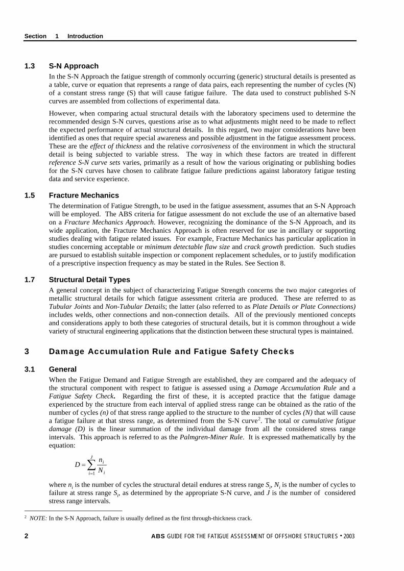
A diagram outlining the fatigue assessment process documented in this Guide is given in Section 1, Figure 1.
FIGURE 1 Schematic of Fatigue Assessment Process
(For each location or structural detail)
FATIGUESTRENGTH/
DAMAGECALCULATION
BASED ONSELECTEDMETHOD
INITIAL FATIGUEASSESSMENT
SELECT Fatigue DesignFactor (FDF)
SECTION 4
OBTAIN NEEDED FRACTUREMECHANICS ANALYSIS
PARAMETERS
SECTION 8
SELECT S-NCURVE
SECTION 3
CLASSIFY DETAIL,CONSIDER STRESS
CONCENTRATION FACTOR& DECIDE APPLICABILITY OF
NOMINAL OR HOT SPOTAPPROACH
SECTION 2
DETERMINISTICMETHOD
SECTION 7
FRACTUREMECHANICS METHOD
SECTION 8
SIMPLIFIEDMETHOD
SECTION 5
SPECTRAL-BASEDMETHOD
SECTION 6
FATIGUESAFETY CHECK
SEE 1/3.5
4 ABS GUIDE FOR THE FATIGUE ASSESSMENT OF OFFSHORE STRUCTURES . 2003
S e c t i o n 2 : F a t i g u e S t r e n g t h B a s e d o n S - N C u r v e s
S E C T I O N 2 Fatigue Strength Based on S-N Curves
1 Introduction
1.1 General This Section describes the procedures that can be followed when the fatigue strength of a structural detail is established using an S-N curve. Section 3 presents the specific data that define the various S-N curves and the required adjustments.
The S-N method and the S-N curves are typically presented as being related to a Nominal Stress Approach or a Hot Spot Stress Approach. The basis and application of these approaches are described below.
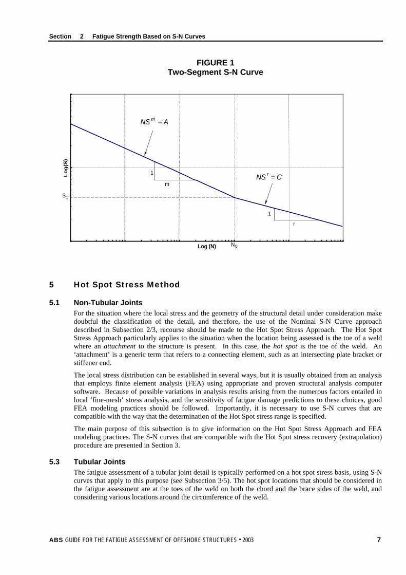
1.3 Defining Parameters Section 2, Figure 1 shows a two-segment S-N curve.
When the number of cycles to failure, N, is less than NQ in Section 2, Figure 1, the relationship between N and stress range (S) is:
N = A ∙ S–m .................................................................................................................................. (2.1)
where A and m are the fatigue strength coefficient and exponent respectively, as determined from fatigue tests.
When N is greater than NQ cycles,
N = C ∙ S–r ................................................................................................................................... (2.2)
where C and r are again determined from fatigue tests.
1.5 Tolerances and Alignments The basis of, and the selection and use of, nominal S-N curves should reflect the tolerance and alignment criteria, and inspection and repair practices employed by the builder. When those actually to be employed exceed the permissible bounds of acceptable industry practice, they are to be fully documented and proven acceptable for the intended application.
3 Nominal Stress Method
3.1 ‘Reference’ Stress and Stress Concentration Factor The nominal stress range for the location where the fatigue assessment is being conducted may need to be modified to account for local conditions that affect the local stress at that location. The ratio of the local to nominal stress is the definition of the Stress Concentration Factor (SCF) already described in Section 1. Depending on specific situations, different SCF may apply to different nominal stress components, and while it is most common to encounter SCF values larger than 1.0, thus signifying an amplification of the nominal stress, there are situations where a value of less than 1.0 can validly exist.
The nominal S-N curves were derived from fatigue test data obtained mainly from specimens subjected to axial and bending loads. The reference stresses used in the S-N curves are the nominal stresses typically calculated based on the applied loading and sectional properties of the specimens.
ABS GUIDE FOR THE FATIGUE ASSESSMENT OF OFFSHORE STRUCTURES . 2003 5
Section 2 Fatigue Strength Based on S-N Curves
Therefore, it is important to recognize that when using these design S-N curves in a fatigue assessment, the applied reference stresses should correspond to the nominal stresses used in creating these curves. However, in an actual structure, it is rare that a match will be found with the geometry and loading of the tested specimens. In most cases, the actual details are more complex than the test specimens, both in geometry and in applied loading, and the required nominal stresses are often not readily available or are difficult to determine. As general guidance, the following may be applied for the determination of the appropriate reference stresses required for a fatigue strength assessment:
i) In cases where the nominal stress approach can be used (e.g., in way of cut-outs or access holes), the reference stresses are the local nominal stresses. The word ‘local’ means that the nominal stresses are determined by taking into account the gross geometric changes of the detail (e.g. cutouts, tapers, haunches, presence of brackets, changes of scantlings, misalignment, etc.).
ii) The effect of stress concentration due to weld profiles should be disregarded. This effect is embodied in the design S-N curves.
iii) Often the S-N curve selected for the structural detail already reflects the effect of a stress concentration due to an abrupt geometric change. In this case, the effect of the stress concentration should be ignored since its effect is implicitly included in the S-N curve.
iv) If the stress field is more complex than a uniaxial field, the principal stress adjacent to potential crack locations should be used.
v) In making a finite element model for the structure, use smooth transitions to avoid abrupt changes in mesh sizes. It is also to be noted that it is unnecessary and often undesirable to use a very fine mesh model to determine the required local nominal stresses.
vi) One exception to the above is with regard to S-N curves that are used in the assessment of transverse load carrying fillet welds where cracking could occur in the weld throat (Detail Class ‘W’ of Appendix 1). In this case, the reference stress is the nominal shearing stress across the minimum weld throat area.
It is to be noted that when the hot spot stress approach is used (see Subsection 2/5 below), an exception should be made with regard to the above items iii) and v). The specified S-N curve used in the hot spot approach will not account for local geometric changes; therefore it will be necessary to perform a structural analysis to determine explicitly the stress concentrations due to such changes. Also in most cases, a finer-mesh finite element model will be required (i.e. approximate finite element analysis mesh size of t × t for shell elements immediately adjacent to the hot spot e.g. weld toe where t is the member thickness).
In addition to the ordinary ‘geometric’ SCF, an additional category of SCF occurs when, at the location where the fatigue assessment is performed, there is a welded ‘attachment’ present. The presence of the welded attachment adds uncertainty about the local stress and the applicable S-N curve at locations in the attachment weld. Many commonly occurring situations of this type are still covered in the nominal stress Joint Classification guidance, such as shown in Appendix 1 (see also 3/3.1.2). However, in the more complex/uncertain cases recourse is made to the hot spot stress approach, which is covered in the next subsection.
6 ABS GUIDE FOR THE FATIGUE ASSESSMENT OF OFFSHORE STRUCTURES . 2003
Section 2 Fatigue Strength Based on S-N Curves
FIGURE 1 Two-Segment S-N Curve
Log (N)
Log(
S)
NS m = A
NS r = C1
m
1
r
SQ
NQ
5 Hot Spot Stress Method
5.1 Non-Tubular Joints For the situation where the local stress and the geometry of the structural detail under consideration make doubtful the classification of the detail, and therefore, the use of the Nominal S-N Curve approach described in Subsection 2/3, recourse should be made to the Hot Spot Stress Approach. The Hot Spot Stress Approach particularly applies to the situation when the location being assessed is the toe of a weld where an attachment to the structure is present. In this case, the hot spot is the toe of the weld. An ‘attachment’ is a generic term that refers to a connecting element, such as an intersecting plate bracket or stiffener end.
The local stress distribution can be established in several ways, but it is usually obtained from an analysis that employs finite element analysis (FEA) using appropriate and proven structural analysis computer software. Because of possible variations in analysis results arising from the numerous factors entailed in local ‘fine-mesh’ stress analysis, and the sensitivity of fatigue damage predictions to these choices, good FEA modeling practices should be followed. Importantly, it is necessary to use S-N curves that are compatible with the way that the determination of the Hot Spot stress range is specified.
The main purpose of this subsection is to give information on the Hot Spot Stress Approach and FEA modeling practices. The S-N curves that are compatible with the Hot Spot stress recovery (extrapolation) procedure are presented in Section 3.
5.3 Tubular Joints The fatigue assessment of a tubular joint detail is typically performed on a hot spot stress basis, using S-N curves that apply to this purpose (see Subsection 3/5). The hot spot locations that should be considered in the fatigue assessment are at the toes of the weld on both the chord and the brace sides of the weld, and considering various locations around the circumference of the weld.
ABS GUIDE FOR THE FATIGUE ASSESSMENT OF OFFSHORE STRUCTURES . 2003 7
Section 2 Fatigue Strength Based on S-N Curves
5.5 Stress Definitions and Related Approaches 5.5.1 Stress Definitions
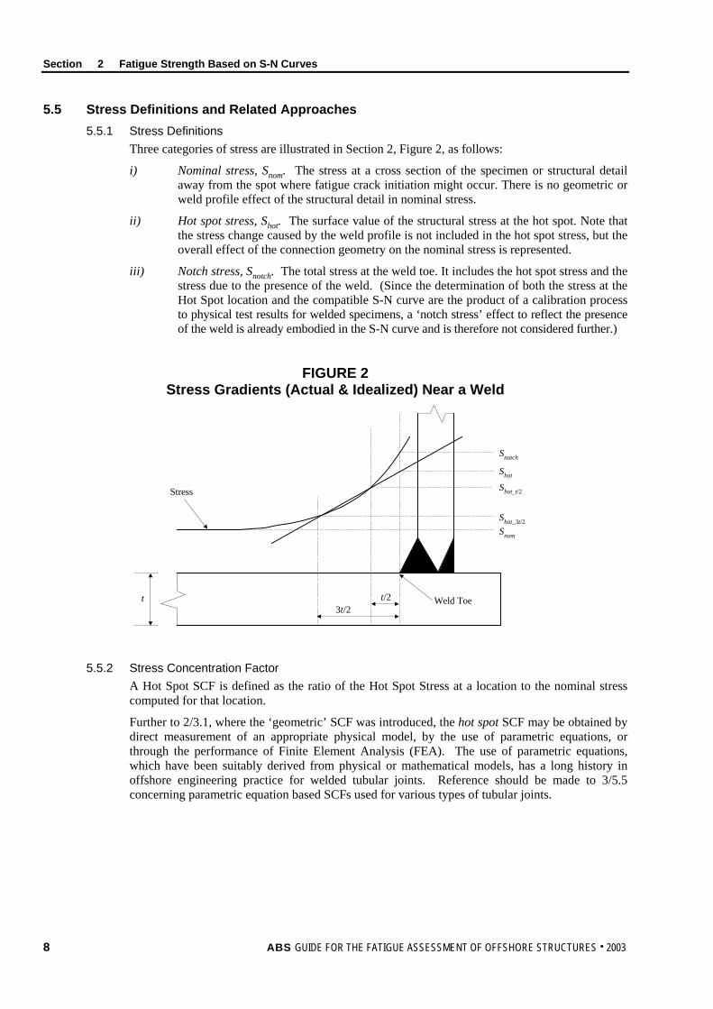
Three categories of stress are illustrated in Section 2, Figure 2, as follows:
i) Nominal stress, Snom. The stress at a cross section of the specimen or structural detail away from the spot where fatigue crack initiation might occur. There is no geometric or weld profile effect of the structural detail in nominal stress.
ii) Hot spot stress, Shot. The surface value of the structural stress at the hot spot. Note that the stress change caused by the weld profile is not included in the hot spot stress, but the overall effect of the connection geometry on the nominal stress is represented.
iii) Notch stress, Snotch. The total stress at the weld toe. It includes the hot spot stress and the stress due to the presence of the weld. (Since the determination of both the stress at the Hot Spot location and the compatible S-N curve are the product of a calibration process to physical test results for welded specimens, a ‘notch stress’ effect to reflect the presence of the weld is already embodied in the S-N curve and is therefore not considered further.)
FIGURE 2 Stress Gradients (Actual & Idealized) Near a Weld
Stress
t3t/2
t/2 Weld Toe
Snom
Shot_3t/2
Shot_t/2
Shot
Snotch
5.5.2 Stress Concentration Factor A Hot Spot SCF is defined as the ratio of the Hot Spot Stress at a location to the nominal stress computed for that location.
Further to 2/3.1, where the ‘geometric’ SCF was introduced, the hot spot SCF may be obtained by direct measurement of an appropriate physical model, by the use of parametric equations, or through the performance of Finite Element Analysis (FEA). The use of parametric equations, which have been suitably derived from physical or mathematical models, has a long history in offshore engineering practice for welded tubular joints. Reference should be made to 3/5.5 concerning parametric equation based SCFs used for various types of tubular joints.
8 ABS GUIDE FOR THE FATIGUE ASSESSMENT OF OFFSHORE STRUCTURES . 2003

Section 2 Fatigue Strength Based on S-N Curves
5.7 Finite Element Analysis to Obtain Hot Spot Stress 5.7.1 General Modeling Considerations
The FEA that needs to be performed to obtain the hot spot stress at each critical location on a structural detail will need to be relatively ‘fine-meshed’ so that an accurate depiction of the acting stress gradient in way of the critical location will be obtained. However, the mesh should not be too fine such that peak stresses due to geometric and other discontinuities will be overestimated. This is especially relevant if the S-N curve used in the fatigue assessment already reflects the presence of a discontinuity such as the weld itself. There are numerous literature references giving examples of successful analyses and appropriate recommendations on modeling practices that should be used to obtain the desired hot spot stress distribution. In the interest of providing an indication of the level and type of analysis envisioned the following modeling guidance is presented.
5.7.1(a) Element Type. Linear elastic quadrilateral plate or shell elements are typically used. The mesh is created at the mid-level of the plate and the weld profile itself is not represented in the model. In special situations, such as where the focus of the analysis is to establish the influence of the weld shape itself, recourse can be made to solid elements. The brick element may be used in this case. The use of triangular elements should be avoided in the hot spot region.
5.7.1(b) Element Size. The element size in way of the hot spot location should be approximately t × t. (See Section 2, Figure 2 regarding the dimension, t.)
5.7.1(c) Aspect Ratio. Ideally, an aspect ratio of 1:1 immediately adjacent to the hot spot location should be used. Away from the hot spot region, the aspect ratio should be ideally limited to 1:3, and any element exceeding this ratio should be well away from the area of interest and then should not exceed 1:5. The corner angles of the quadrilateral plate or shell elements should be confined to the range 50 to 130 degrees.
5.7.1(d) Gradation of the Mesh. The change in mesh size from the finest at the hot spot to coarser gradations away from the hot spot region should be accomplished in a smooth and uniform fashion. Immediately adjacent to the hot spot, it is suggested that several of the elements leading into the hot spot location should be the same size.
5.7.1(e) Stresses of Interest. The hot spot stress approach relies on a linear extrapolation scheme, where ‘reference’ stresses at each of two locations adjacent to the hot spot location are extrapolated to the hot spot.
5.9 FEA Data Interpretation – Stress Extrapolation Procedure and S-N Curves 5.9.1 Non-tubular Welded Connections
Section 2, Figure 2 shows an acceptable method, which can be used to extract and interpret the ‘weld toe’ hot spot stress and to obtain a linearly extrapolated stress at the weld toe. According to the Figure, the weld’s hot spot stress can be determined by a linear extrapolation to the weld toe using the calculated ‘reference’ stress at t/2 and 3t/2 from weld toe. When stresses are obtained in this manner, the use of the ABS Offshore S-N Curve-Joint Class ‘E’ curve is recommended (see Subsection 3/3).
When the finite element analysis employs the plate or shell element idealization of 2/5.7, the ‘reference’ stresses are the element component stresses obtained for the element’s surface that is on the plane containing the line along the weld toe. Each main surface stress component for both of the specified distances from the weld toe is individually extrapolated to the weld toe location. (The main stress components referred to here are typically – the two orthogonal local coordinate normal stresses and the corresponding shear stress; usually denoted σx, σy, τxy). Then the extrapolated component stresses are used to compute the maximum principal stress at the weld toe. The maximum principal stress at the hot spot, determined in this fashion, should be used in the fatigue assessment.4
4 NOTE: When the angle between the normal to the weld’s axis and the direction of the maximum principal stress at the hot spot is greater than 45 degrees, consideration may be given to an appropriate reduction of the maximum principal stress used in the fatigue assessment.
ABS GUIDE FOR THE FATIGUE ASSESSMENT OF OFFSHORE STRUCTURES . 2003 9

Section 2 Fatigue Strength Based on S-N Curves
A refined linear extrapolation procedure to obtain the hot spot stress, using the mentioned distances from the hot spot, may be accomplished following the procedure given in the ABS Steel Vessel Rules, Part 5C, Chapter 1, Appendix 1/13.7.
5.9.2 Tubular Joints In general, the use of parametric SCF equations is preferred to determine the SCFs at welded tubular connections. Where appropriate parametric equations based SCFs (See 3/5.5 and Appendix 2) are not available, recourse should be made to a suitable FEA to determine the applicable SCFs. In this case, the extrapolation procedure is similar to that for non-tubular welded connections.
10 ABS GUIDE FOR THE FATIGUE ASSESSMENT OF OFFSHORE STRUCTURES . 2003
S e c t i o n 3 : S - N C u r v e s
S E C T I O N 3 S-N Curves
1 Introduction This section presents the various S-N curves that can be used in a fatigue assessment. Subsection 3/3 addresses the S-N curves for non-tubular details using the nominal stress method. Subsection 3/5 primarily addresses the S-N curves which can be applied to tubular joints.
3 S-N Curves and Adjustments for Non-Tubular Details (Specification of the Nominal Fatigue Strength Criteria)
3.1 ABS Offshore S-N Curves 3.1.1 General
The ABS Offshore S-N Curves for non-tubular details (and non-intersection tubular connections) are defined according to the geometry of the detail and other considerations such as the direction of loading and expected fabrication/ inspection methods. The S-N curves are presented in various categories each representing a class of details (most of which are welded connection details) as discussed in 3/3.1.2 on ‘Joint Classification’. Section 3, Tables 1, 2 and 3 provide the defining parameters for the ABS Offshore S-N Curves applicable to various classes of non-tubular details. These Tables apply when the long-term environmental conditions (referred to here as, ‘corrosiveness’), that the structural detail will experience, are represented as being: ‘In –Air’ (A), ‘Cathodically Protected’ (CP), and ‘Freely Corroding’ (FC).
The three ‘corrosiveness’ situations for the ABS Offshore S-N Curves are denoted as:
ABS- (A) for the ‘In –Air’ condition
ABS- (CP) for the ‘Cathodic Protection’ condition, and
ABS- (FC) for the ‘Free Corrosion’ condition
Section 3, Figures 1, 2 and 3, respectively, show the S-N curves given in Section 3, Tables 1, 2 and 3.
3.1.2 Joint Classification The S-N curves categorize structural details into one of eight ‘nominal’ classes: denoted B, C, D, E, F, F2, G, and W. The classification of a detail requires appropriately matching it to the most applicable one of these nominal classes while considering the potential cracking locations in the detail and the direction of the applied loading.
An example of the preferred convention to refer to the particular S-N curve applicable to a detail would be: ABS- (A) Detail Class ‘F2’.
Appendix 1 provides guidance on the classification of structural details in accordance with the ABS Offshore S-N Curves. Note: Something that often confuses the classification of a detail is the desire to force the assignment of the
detail into one of the ‘nominal’ classes. It frequently happens that the complex geometry of a detail or local stress distribution makes the classification to one of the available classes inappropriate or too doubtful. In this case recourse should be made to the techniques discussed in Subparagraph 2/5.9.1.
ABS GUIDE FOR THE FATIGUE ASSESSMENT OF OFFSHORE STRUCTURES . 2003 11
Section 3 S-N Curves
3.1.3 Adjusting S-N Curves for Corrosive Environments The ‘In-Air’ (A) S-N curves are modified for ‘Cathodic Protection’ (CP)’ and ‘Free Corrosion’ (FC) conditions in seawater. Refer to Section 3, Tables 1, 2 and 3, which apply, respectively, to the three mentioned conditions. Note: For high strength steels with yield strengths σy > 400 MPa, the indicated adjustment between the ‘In-Air’
and the others conditions needs to be specially considered.
3.1.4 Adjustment for the Effect of Plate Thickness The fatigue performance of a structural detail depends on member thickness. For the same stress range the detail’s fatigue strength may decrease, as the member thickness increases. This effect (also called the ‘scale effect’) is caused by the local geometry of the weld toe in relation to the thickness of the adjoining plates and the stress gradient over the thickness. The basic design S-N curves are applicable to thicknesses that do not exceed the reference thickness tR = 22 mm (7/8 in). For members of greater thickness, the following thickness adjustment to the S-N curves applies:
Sf = S
q
Rtt
−
................................................................................................................ (3.1)
where
S = unmodified stress range in the S-N curve
t = plate thickness of the member under assessment
q = thickness exponent factor (= 0.25)
3.3 AWS S-N Curves for Non-Tubular Details5 The AWS S-N Curves may be permitted for the nominal fatigue assessment of applicable structural details located in ‘above water structure’ (defined under Appendix 3, Table 1). The specification of the S-N curves, structural detail classifications, and applicable adjustments are to comply with the AWS Structural Welding Code, D1.1, 2002.
5 NOTE: The application of these S-N curves is meant for use with Appendix 3.
12 ABS GUIDE FOR THE FATIGUE ASSESSMENT OF OFFSHORE STRUCTURES . 2003

Section 3 S-N Curves
TABLE 1 Parameters for ABS-(A) Offshore S-N Curves for Non-Tubular Details in Air
Curve Class
A m C r NQ SQ For MPa
Units For ksi Units
For MPa Units
For ksi Units
For MPa Units
For ksi Units
B 1.01×10¹⁵ 4.48×10¹¹ 4.0 1.02×10¹⁹ 9.49×10¹³ 6.0 1.0×10⁷ 100.2 14.5 C 4.23×10¹³ 4.93×10¹⁰ 3.5 2.59×10¹⁷ 6.35×10¹² 5.5 1.0×10⁷ 78.2 11.4 D 1.52×10¹² 4.65×10⁹ 3.0 4.33×10¹⁵ 2.79×10¹¹ 5.0 1.0×10⁷ 53.4 7.75 E 1.04×10¹² 3.18×10⁹ 3.0 2.30×10¹⁵ 1.48×10¹¹ 5.0 1.0×10⁷ 47.0 6.83 F 6.30×10¹¹ 1.93×10⁹ 3.0 9.97×10¹⁴ 6.42×10¹⁰ 5.0 1.0×10⁷ 39.8 5.78
F2 4.30×10¹¹ 1.31×10⁹ 3.0 5.28×10¹⁴ 3.40×10¹⁰ 5.0 1.0×10⁷ 35.0 5.08 G 2.50×10¹¹ 7.64×10⁸ 3.0 2.14×10¹⁴ 1.38×10¹⁰ 5.0 1.0×10⁷ 29.2 4.24 W 1.60×10¹¹ 4.89×10⁸ 3.0 1.02×10¹⁴ 6.54×10⁹ 5.0 1.0×10⁷ 25.2 3.66
FIGURE 1 ABS-(A) Offshore S-N Curves for Non-Tubular Details in Air
ABS GUIDE FOR THE FATIGUE ASSESSMENT OF OFFSHORE STRUCTURES . 2003 13
Section 3 S-N Curves
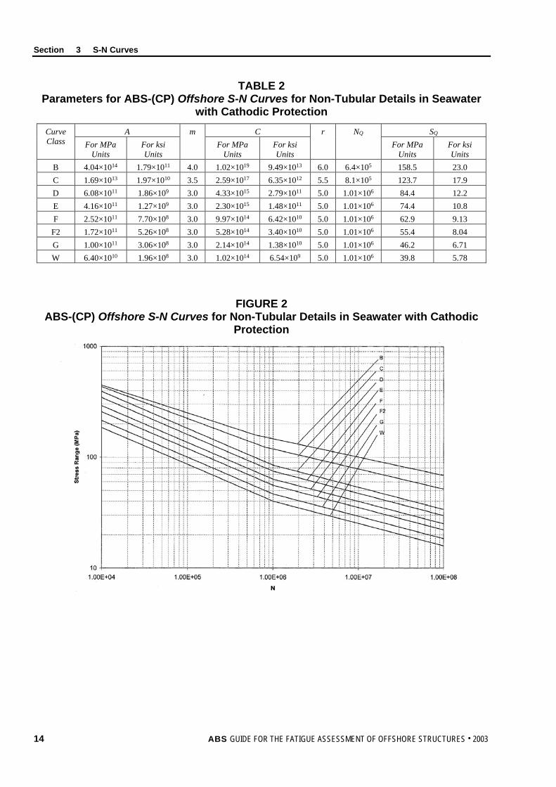
TABLE 2 Parameters for ABS-(CP) Offshore S-N Curves for Non-Tubular Details in Seawater
with Cathodic Protection Curve Class
A m C r NQ SQ For MPa
Units For ksi Units
For MPa Units
For ksi Units
For MPa Units
For ksi Units
B 4.04×10¹⁴ 1.79×10¹¹ 4.0 1.02×10¹⁹ 9.49×10¹³ 6.0 6.4×10⁵ 158.5 23.0 C 1.69×10¹³ 1.97×10¹⁰ 3.5 2.59×10¹⁷ 6.35×10¹² 5.5 8.1×10⁵ 123.7 17.9 D 6.08×10¹¹ 1.86×10⁹ 3.0 4.33×10¹⁵ 2.79×10¹¹ 5.0 1.01×10⁶ 84.4 12.2 E 4.16×10¹¹ 1.27×10⁹ 3.0 2.30×10¹⁵ 1.48×10¹¹ 5.0 1.01×10⁶ 74.4 10.8 F 2.52×10¹¹ 7.70×10⁸ 3.0 9.97×10¹⁴ 6.42×10¹⁰ 5.0 1.01×10⁶ 62.9 9.13
F2 1.72×10¹¹ 5.26×10⁸ 3.0 5.28×10¹⁴ 3.40×10¹⁰ 5.0 1.01×10⁶ 55.4 8.04 G 1.00×10¹¹ 3.06×10⁸ 3.0 2.14×10¹⁴ 1.38×10¹⁰ 5.0 1.01×10⁶ 46.2 6.71 W 6.40×10¹⁰ 1.96×10⁸ 3.0 1.02×10¹⁴ 6.54×10⁹ 5.0 1.01×10⁶ 39.8 5.78
FIGURE 2 ABS-(CP) Offshore S-N Curves for Non-Tubular Details in Seawater with Cathodic
Protection
14 ABS GUIDE FOR THE FATIGUE ASSESSMENT OF OFFSHORE STRUCTURES . 2003

Section 3 S-N Curves
TABLE 3 Parameters for ABS-(FC) Offshore S-N Curves for Non-Tubular Details in Seawater
for Free Corrosion Curve Class
A m For MPa
Units For ksi Units
B 3.37×10¹⁴ 1.49×10¹¹ 4.0 C 1.41×10¹³ 1.64×10¹⁰ 3.5 D 5.07×10¹¹ 1.55×10⁹ 3.0 E 3.47×10¹¹ 1.06×10⁹ 3.0 F 2.10×10¹¹ 6.42×10⁸ 3.0
F2 1.43×10¹¹ 4.38×10⁸ 3.0 G 8.33×10¹⁰ 2.55×10⁸ 3.0 W 5.33×10¹⁰ 1.63×10⁸ 3.0
FIGURE 3 ABS-(FC) Offshore S-N Curves for Non-Tubular Details in Seawater for Free
Corrosion
ABS GUIDE FOR THE FATIGUE ASSESSMENT OF OFFSHORE STRUCTURES . 2003 15

Section 3 S-N Curves
5 S-N Curves for Tubular Joints
5.1 ABS Offshore S-N Curves 5.1.1 General
The ABS S-N Curves for tubular intersection joints are denoted as:
ABS - T(A) for the ‘In-Air’ condition
ABS - T(CP) for the ‘Cathodic Protection’ condition
ABS - T(FC) for the ‘Free Corrosion’ condition
The ABS - T(A) curve is defined by parameters A and m, which are defined for Eq. (2.1), and the parameters r and C, defined for Eq. (2.2). This ‘T’ curve has a change of slope at 107 cycles.
5.1.2 Adjustment for Corrosive Environments The ABS - T(A) is modified for ‘Cathodic Protection’ (CP)’ and ‘Free Corrosion’ (FC) conditions. Refer to Section 3, Table 4, which applies, respectively, to the three mentioned conditions, and Section 3, Figure 4, depicts the curves.
5.1.3 Adjustment for Thickness The basic ‘T’ curve is applicable to member thickness up to 22 mm (7/8 in.). For members of greater thickness, Eq. (3.1) applies, using the reference thickness tR = 32 mm (11/4 in) with the thickness exponent factor (q) equal to 0.25. Note: This gives a benefit for nodal joints with wall thickness between 22 and 32 mm (7/8 and 11/4 in.).
16 ABS GUIDE FOR THE FATIGUE ASSESSMENT OF OFFSHORE STRUCTURES . 2003

Section 3 S-N Curves
TABLE 4 Parameters for Class ‘T’ ABS Offshore S-N Curves
S-N Curve
A m C r NQ SQ For MPa
Units For ksi Units
For MPa Units
For ksi Units
For MPa Units
For ksi Units
T(A) 1.46×10¹² 4.46×10⁹ 3.0 4.05×10¹⁵ 2.61×10¹¹ 5.0 1.0×10⁷ 52.7 7.64 T(CP) 7.30×10¹¹ 2.23×10⁹ 3.0 4.05×10¹⁵ 2.61×10¹¹ 5.0 1.77×10⁶ 74.5 10.8 T(FC) 4.87×10¹¹ 1.49×10⁹ 3.0 -- -- -- -- -- --
Note: For service in seawater with free corrosion (FC), there is no change in the curve slope.
FIGURE 4 ABS Offshore S-N Curves for Tubular Joints (in air, in seawater with cathodic
protection and in seawater for free corrosion)
5.3 API S-N Curves6 5.3.1 General
As per API RP-2A (WSD-21st Edition, 12/ 2000) the S-N curves for tubular intersections (API X and X′) are defined in Section 3, Table 5. The parameters A and m are defined for Eq. (2.1).
5.3.2 Use of the X′ Curve The X′ curve is applicable for welds without profile control that conform to a basic standard flat profile (Ref: AWS D1.1.2002, Figure 3.8) and has a branch thickness less than 16 mm (5/8 in). For greater wall thickness, the following thickness adjustment should be applied.
6 NOTE: The application of these S-N curves is meant for use with Appendix 3.
ABS GUIDE FOR THE FATIGUE ASSESSMENT OF OFFSHORE STRUCTURES . 2003 17
Section 3 S-N Curves
The fatigue strength, Sf, is:
Sf = S
25.0−
Rtt ............................................................................................................. (3.2)
where
S = allowable stress from the S-N curve
t = branch member thickness
tR = limiting branch thickness
5.3.3 Use of the X Curve The X curve is applicable to welds with profile control and having a branch thickness less than 25 mm (1 in). For the same controlled profile at a greater thickness, the thickness adjustment of Eq. (3.2) should be used. However, reductions below the X′ Curve are not required. The X curve may be used without the thickness adjustment, provided the profile is ground smooth to a radius greater than or equal to half the branch thickness. Final grinding marks should be transverse to the weld axis and the entire finished profile should pass magnetic particle inspection (MPI).
It is emphasized that the use of the X curve is contingent on the satisfactory performance and results of 100 percent MPI of the weld. The acceptance in the design review of the X curve may be reserved pending submission of acknowledgment that the fabricator can and will provide the required weld profiling, grinding marks and inspections.
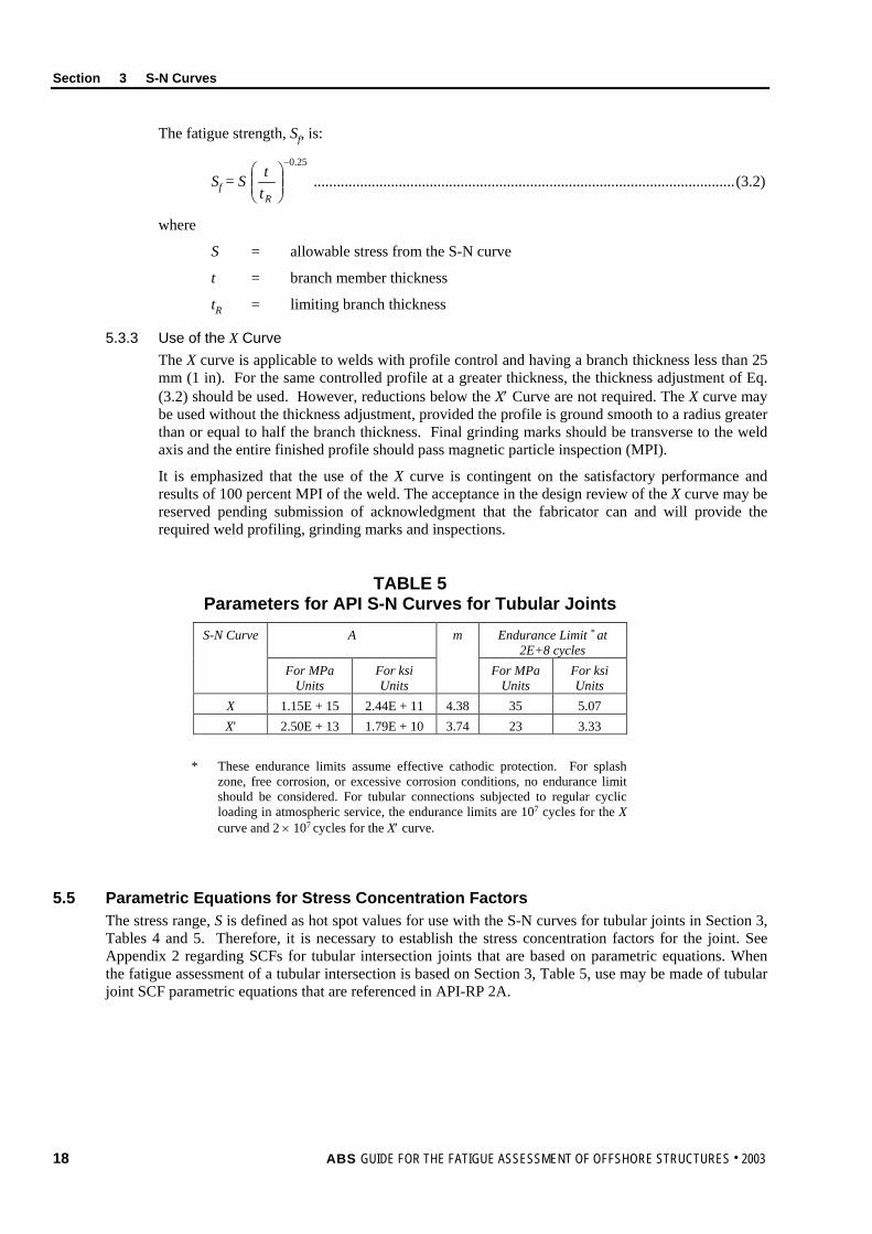
TABLE 5 Parameters for API S-N Curves for Tubular Joints S-N Curve A m Endurance Limit * at
2E+8 cycles For MPa
Units For ksi Units
For MPa Units
For ksi Units
X 1.15E + 15 2.44E + 11 4.38 35 5.07 X' 2.50E + 13 1.79E + 10 3.74 23 3.33
* These endurance limits assume effective cathodic protection. For splash zone, free corrosion, or excessive corrosion conditions, no endurance limit should be considered. For tubular connections subjected to regular cyclic loading in atmospheric service, the endurance limits are 107 cycles for the X curve and 2 × 10⁷ cycles for the X′ curve.
5.5 Parametric Equations for Stress Concentration Factors The stress range, S is defined as hot spot values for use with the S-N curves for tubular joints in Section 3, Tables 4 and 5. Therefore, it is necessary to establish the stress concentration factors for the joint. See Appendix 2 regarding SCFs for tubular intersection joints that are based on parametric equations. When the fatigue assessment of a tubular intersection is based on Section 3, Table 5, use may be made of tubular joint SCF parametric equations that are referenced in API-RP 2A.
18 ABS GUIDE FOR THE FATIGUE ASSESSMENT OF OFFSHORE STRUCTURES . 2003

Section 3 S-N Curves
7 Cast Steel Components A cast steel component that is fabricated in accordance with an acceptable standard may be used to resist long-term fatigue loadings. The fatigue strength should be based on the S-N curve given in Section 3, Figure 5, which represent the ‘in air’ condition. The parameters of this curve are given in Section 3, Table 6. When the cast steel component is used in a submerged structure with normal cathodic protection conditions, a factor of 2 should be applied to reduce the ordinates of the ‘in-air’ S-N curve.
The effect of casting thickness should be taken into account, using the approach given in 3/3.1.4. In Eq. (3.1), the reference thickness should be 38 mm (11/2 in.) and the exponent 0.15.
To verify the position of the maximum stress range in the casting it is recommended that a finite element analysis should be undertaken for fatigue sensitive joints. For the particular case of cast tubular nodal connections, it is important to note that the brace to casting circumferential butt weld may become the most critical location for fatigue.
TABLE 6 Parameters for ABS Offshore S-N Curve for Cast Steel Joints (in-air)
Curve Class
A m For MPa
Units For ksi Units
CS 1.48×10¹⁵ 6.56×10¹¹ 4.0
FIGURE 5 ABS Offshore S-N Curve for Cast Steel Joints (in-air)
ABS GUIDE FOR THE FATIGUE ASSESSMENT OF OFFSHORE STRUCTURES . 2003 19

S e c t i o n 4 : F a t i g u e D e s i g n F a c t o r s
S E C T I O N 4 Fatigue Design Factors
1 General The Fatigue Design Factor (FDF) is a parameter with a value of 1.0 or more, which is applied to increase the required design fatigue life or to decrease the calculated permissible fatigue damage; see 1/3.5. Section 4, Table 1 presents the FDF values for various types of offshore structures, structural details, detail locations and other considerations. The ‘Notes for Table 1’, listed after the table, must be observed when using the table.
Designers and Analysts are advised that a cognizant Regulatory Authority for the Offshore Structure may have required technical criteria that could be different from those stated herein. ABS will consider the use of such alternative criteria as a basis of Classification where it is shown that the use of the alternative criteria produces a level of safety that is not less than that produced by the criteria given herein. Ordinarily the demonstration of an alternative’s acceptability is done by the designer’s submission of comparative calculations that appropriately consider the pertinent parameters (including loads, S-N curve data, FDFs, etc.) and calculation methods specified in the alternative criteria. However, where satisfactory experience exists with the use of the regulatory mandated alternative criteria, they may be accepted for classification after consideration of the claimed experience by ABS and consultation with the structure’s Operator. An example of acceptable alternative criteria, for a steel Offshore Structure located on the Outer Continental Shelf (OCS) of the United States, are the fatigue design requirements cited in the technical criteria issued by Minerals Management Service (MMS). For the use of U.S. OCS platform clients, an alternative version of Table 1 is presented in Appendix 3 of this Guide.
20 ABS GUIDE FOR THE FATIGUE ASSESSMENT OF OFFSHORE STRUCTURES . 2003

Section 4 Fatigue Design Factors
TABLE 1 Fatigue Design Factors for Structural Details**
** The minimum Factor to be applied to uninspectable ‘ordinary’ or uninspectable ‘critical’ structural details is 5 or 10, respectively.
STRUCTURAL DETAIL (3) GOVERNING FATIGUE STRENGTH
CRITERIA
APPLICATION (1) CATEGORY**
LOCATION ORDINARY CRITICAL (2) Structural Subsystem (4) Type
FIXED & FLOATING INSTALLATION ABOVE WATER STRUCTURE Non-Integral Deck (5) Non Tubular (7) ABS-(A) 1 2
Tubular Intersection (8)
ABS-T(A) 1 2
Integral Deck (6) Non Tubular ABS- (A) 2 3 Tubular Intersection
ABS-T(A) 2 3
IN WATER & SUBMERGED STRUCTURE (9) Fixed Non-Floating Structure (e.g. fixed jacket, tower and template)
Non Tubular ABS- (CP) (16) 2 3 Tubular Intersection
ABS- T(CP) (16) 2 3
Fixed Floating Structure (e.g. TLP, Column Stabilized & SPAR; but excluding Ship-type & MODU (14))
Non Tubular (10) ABS- (CP) 3 5 Tubular Intersection
ABS-T(CP) 3 5
FOUNDATION COMPONENTS (12) ABS- (CP) or ABS-T(CP)
NA NA
10 10
MOORING COMPONENTS (13) ABS FPI Guide (11) NA 3 TLP TENDON (13) See Note 15 NA 10
NOTES for TABLE 1 1 The stated Factors presume that the detail can be inspected at times of anticipated scheduled survey or when structural
damage is suspected. The need to move equipment or covers to provide direct visual access or to employ inspection tools does not disqualify the detail as being ‘inspectable’. However where the ability to perform direct visual inspection is not evident from the submitted design documentation, any ‘Inspection Plan’ as required by the applicable Rules is to address how it is intended that the required, effective inspection will be accomplished. The use of uninspectable details should be avoided as far as is practicable.
2 A detail is considered critical if its failure will cause the rapid loss of structural integrity AND this produces an event of unacceptable consequence (e.g. loss of life; pollution; loss of platform; collision damage to another structure, facility, or important natural feature). In this context ‘rapid’ means that even a very local failure can not be detected, inspected and repaired
• before the occurrence of a broader, catastrophic structural failure, or
• before steps can be taken to eliminate any potential unacceptable consequence.
The designer is responsible to identify all potentially ‘critical’ structural details and to advise what rationale is being taken if the detail is being categorized as ‘ordinary’ (i.e. a detail that is redundant having a lower failure consequence).
3 ‘Structural Detail’ refers to both welded connections and non-welded details.
4 At an interface connection between structural subsystems, the higher (more demanding) of the two applicable requirements shall apply on both sides of the interface connection.
5 ‘Non-Integral Deck Structure’ means the deck is not essential for the structural integrity of the structural subsystem supporting the deck.
ABS GUIDE FOR THE FATIGUE ASSESSMENT OF OFFSHORE STRUCTURES . 2003 21

Section 4 Fatigue Design Factors
6 ‘Integral Deck Structure’ means the deck structure is an essential component of the structural integrity of the overall platform structure [e.g. the deck structure spanning the columns of a TLP or a Column Stabilized type platform.]
7 ‘Non-Tubular’ means both non-tubular details (also called ‘plate details’) and non-intersecting tubular details (e.g. butt joints of tubular members and attachments to tubular members)
8 ‘Tubular Intersection’ refers to the nodal connections of tubular brace (branch) members with a tubular chord member.
9 This region is defined as being from the top of the air-gap down to the seabed and beneath to the bottom of the foundation elements (e.g. pile tips). But, for a non-integral deck and for the purposes of the fatigue assessment only, this region can be defined as being from the ‘deck to jacket (or hull) connection’ down to (and below) the seabed.
10 Internal structural tanks that are used for the (non-permanent) storage of seawater may be designed to the ABS- (A) criteria provided:
• complete recoating is planned to occur in or before the 10th year of structural life,
• an effective coating system is provided to the entire tank (to be considered effective, there should be appropriate surface preparation prior to coating, appropriate application and monitoring of a 2 coat epoxy coating, or at least an equally effective coating),
• the space is accessible for close-up visual inspection to assess coating condition, and
• arrangements are provided to perform local coating renewal at weld detail locations.
11 Refer to API RP 2SK concerning the components and criteria to be assessed.
12 The factor listed is applicable to the in-place condition. Other criteria may be considered when assessing the installation condition.
13 The appropriate criteria to be used for cast structural components will be specially considered.
14 The fatigue assessment of a MODU (e.g. Column Stabilized and Self Elevating types) typically employs the ABS (A) or (CP) criteria, as applicable, with a Fatigue Design Factor of 1.0 for the structural details required by the MODU Rules to undergo a fatigue assessment.
15 Requires special consideration. For guidance use may be made of AWS C1 or API X S-N data for tendon girth welds, but note AWS criteria may have limitations regarding available geometry, material thickness and corrosiveness. The acceptability of these AWS and API S-N curves requires very high quality NDT of the welds, and appropriate corrosion protection via coating, cathodic protection or both.
16 In the ‘splash zone’ (see Offshore Installations Rules 3-2-4/5.9.2), the use of the ABS (FC) S-N data may be required.
22 ABS GUIDE FOR THE FATIGUE ASSESSMENT OF OFFSHORE STRUCTURES . 2003

ABS GUIDE FOR THE FATIGUE ASSESSMENT OF OFFSHORE STRUCTURES . 2003 23
S e c t i o n 5 : T h e S i m p l i f i e d F a t i g u e A s s e s s m e n t M e t h o d
S E C T I O N 5 The Simplified Fatigue Assessment Method
1 Introduction The so-called ‘simplified’ method is also sometimes referred to as the ‘permissible’ or ‘allowable’ stress range method, which can be categorized as an indirect fatigue assessment method because the result of the method’s application is not necessarily a value of fatigue damage or a fatigue life value. Often a ‘pass/fail’ answer results depending on whether the acting stress range is below or above the permissible value.
This method is often used as the basis of a fatigue screening technique. A screening technique is typically a rapid, but usually conservatively biased, check of structural adequacy. If the structure’s strength is adequate when checked with the screening criterion, no further analysis may be required. If the structural detail fails the screening criterion, the proof of its adequacy may still be pursued by analysis using more refined techniques. Also, a screening approach is quite useful to identify fatigue sensitive areas of the structure, thus providing a basis to develop fatigue inspection planning for future periodic inspections of the structure and Condition Assessment surveys of the structure.
3 Mathematical Development
3.1 General Assumptions In the simplified fatigue assessment method, the two-parameter Weibull distribution is used to model the long-term distribution of fatigue stresses. The cumulative distribution function of the stress range can be expressed as:
Fs(S) = 1 – exp
S
, S > 0 .............................................................................................. (5.1)
where
S = a random variable denoting stress range
= the Weibull shape parameter
= the Weibull scale parameter
Based on the long-term distribution of stress range, a closed form expression for fatigue damage can be derived. A major feature of the simplified method is that appropriate application of experience data can be made to establish or estimate the Weibull shape parameter, thus avoiding a lengthy spectral analysis.
The other major assumptions underlying the simplified approach are that the linear cumulative damage (Palmgren-Miner) rule applies, and that fatigue strength is defined by the S-N curves.
3.3 Parameters in the Weibull Distribution
The scale parameter, , which is also called the ‘characteristic value’ of the distribution, is obtained as follows.
Define a ‘reference’ stress range, SR, which characterizes the largest stress range anticipated in a reference number of stress cycles, NR. The probability statement for SR is:
P(S > SR) = RN
1 ......................................................................................................................... (5.2)

Section 5 The Simplified Fatigue Assessment Method
where
NR = number of cycles in a referenced period of time
SR = value which the fatigue stress range exceeds on average once every NR cycles.
For a particular offshore site, the selection of an NR and the determination of the corresponding value of SR can be obtained from empirical data or from long-term wave data (using wave scatter diagram) coupled with appropriate structural analysis.
From the definition of the distribution function, it follows from Eqs. (5.1) and (5.2) that:
γδ /1)(ln R
R
NS
= ........................................................................................................................... (5.3)
The shape parameter, γ, can be established from a detailed stress spectral analysis or its value may be assumed based on experience.
The results of the simplified fatigue assessment method can be very sensitive to the values of the Weibull shape parameter. Therefore, where there is a need to refine the accuracy of the selected shape parameters, the performance of even a basic level global response analysis can be very useful in providing more realistic values. Alternatively, it is suggested that when the basis for the selection of a shape factor is not well known, then a range of probable shape factor values should be employed so that a better appreciation of how selected values affect the fatigue assessment will be obtained.
3.5 Fatigue Damage for the Single Segment S-N Curve Consider the bilinear S-N curve of Section 2, Figure 1. Assume that the left segment, defined by m and A, is extrapolated into the high number of cycles range down to S = 0; i.e., there is no slope change at 107 cycles. (Such a single segment curve would be used for the case of free corrosion in seawater for tubular and non-tubular details.)
For the single segment case, the cumulative fatigue damage can be expressed as:
+Γ= 1
γδ mA
ND
mT ................................................................................................................. (5.4)
where NT is the design life in cycles and Γ(x) is the gamma function, defined as:
∫∞ −−=Γ
0
1)( dtetx tx ..................................................................................................................... (5.5)
3.7 Fatigue Damage for the Two Segment S-N Curve The cumulative fatigue damage for the two-segment case of Section 2, Figure 1 is expressed as:
+Γ+
+Γ= zr
CN
zmA
ND
rT
mT ,1,1 0 γ
δγ
δ .......................................................................... (5.6)
For symbols refer to Section 2, Figure 1 and Subsection 5/3.5. Γ(a,z) and Γ0(a,z) are incomplete gamma functions (integrals z to ∞ and 0 to z, respectively). Values of these functions may be obtained from handbooks.
∫∞ −− Γ−Γ==Γz
ta zaadtetza ),()(),( 01 ...................................................................................... (5.7)
∫ −−=Γz ta dtetza
0
10 ),( ................................................................................................................. (5.8)
γ
δ
= QS
z .................................................................................................................................. (5.9)
where SQ is the stress range at which the slope of the S-N curve changes.
24 ABS GUIDE FOR THE FATIGUE ASSESSMENT OF OFFSHORE STRUCTURES . 2003
Section 5 The Simplified Fatigue Assessment Method
3.9 Allowable Stress Range An alternative way to characterize fatigue strength is in terms of a maximum allowable stress range. This can be done to include consideration of the Fatigue Design Factors (FDF), defined in 1/3.2. Letting D = ∆ = 1/FDF in Eq. (5.6), the maximum allowable stress range, RS ′ , at the probability level corresponding to NR is found as
m
mrT
mR
R
CzrAzmNFDF
NS
/1
0
/
,1,1
)(ln
+Γ+
+Γ⋅
=′−
γδ
γ
γ
............................................ (5.10)
Note that an iterative method is needed to find RS ′ because δ also depends on RS ′ .
The following relationship can be used to find the allowable stress range corresponding to another number of cycles, NS:
γ/1
lnln
′=′
R
SRS N
NSS ................................................................................................................. (5.11)
3.11 Fatigue Safety Check When the fatigue damage is determined in terms of damage ratio, D, as in 5/3.5 or 5/3.7, the safety check is performed according to 1/3.5.
When the fatigue is assessed in terms of allowable stress range as in 5/3.9, the safety check expression corresponding to Eq. 5.10 is:
SR ≤ RS ′ (5.12)
Or if the allowable stress range is modified to reflect a different number of cycles, NS, the safety check is:
SS ≤ SS ′ (5.13)
In practice, it is likely that NR will be based on the Design Life so that the acting reference stress range and maximum allowable stress range (SR and RS ′ ) will refer to NT.
5 Application to Jacket Type Fixed Offshore Installations The simplified method is widely used in Offshore Engineering. For the commonly occurring steel jacket type platform, and similar structural types that meet the application criteria of API RP 2A, significant effort has been expended over the years to calibrate the simplified fatigue assessment method contained in API RP 2A so that it will serve as an appropriate basis for the fatigue design of such structures. When applicable, ABS recognizes the RP 2A ‘simplified method’ as an acceptable basis to perform the fatigue assessment for a fixed platform submitted for ABS Classification.
The use of the RP 2A simplified fatigue assessment criteria for a jacket structure at offshore sites where it is shown that the long-term fatigue inducing effects of the environment are equal to, or less severe than, Gulf of Mexico sites allows its use in these situations as well.
It may not be prudent to use this assessment method as the only basis to judge the acceptability of a design in deeper water [i.e. water depths greater than 120 m. (400 ft.)] because of possibly significant dynamic amplification, or in areas with environmental actions that will have greater fatigue inducing potential. In such cases the method can be employed as a ‘screening’ tool to help identify and prioritize fatigue sensitive areas of the jacket structure. However, it would be expected that the fatigue assessment will ultimately be based on a direct calculation method; and this most likely should be a spectral-based fatigue assessment. The spectral-based method of fatigue assessment is discussed in the next section.
ABS GUIDE FOR THE FATIGUE ASSESSMENT OF OFFSHORE STRUCTURES . 2003 25

S e c t i o n 6 : T h e S p e c t r a l - b a s e d F a t i g u e A s s e s s m e n t M e t h o d
S E C T I O N 6 The Spectral-based Fatigue Assessment Method
1 General A spectral-based fatigue assessment produces results in terms of fatigue induced damage or fatigue life, and it is therefore referred to as a direct method. With ocean waves considered the main source of fatigue demand, the fundamental task of a spectral fatigue analysis is the determination of the stress range transfer function, Hσ(ω|θ), which expresses the relationship between the stress, σ, at a particular structural location per ‘unit wave height,’ and wave of frequency (ω) and heading (θ).
Spectral-based Fatigue Analysis is a complex and numerically intensive technique. As such there is more than one variant of the method that can be validly applied in a particular case. The method is most appropriate when there exists a linear relationship between wave height and the wave-induced loads, and the structural response to these loads is linear. Adaptations to the basic method have been developed to account for various non-linearities, but where there is doubt about the use of such methods, recourse can be made to Time-Domain Analysis Methods as mentioned in Subsection 6/9.
3 Floating Offshore Installations For Column-stabilized and similar structures with large (effective) diameter structural elements, the wave and current induced load components are not dominated by the drag component. Then a linear relationship between wave height and stress range exists. In such a case, the method described Subsection 6/7 may be employed.
5 Jacket Type Fixed Platform Installations For a jacket type platform, because of the typical sizes of the submerged structural elements, the wave and wave with current induced loads are likely to be drag-dominated, thus requiring a structural analysis method that will linearize the hydrodynamic loads, or the transfer function. If the dynamic response characteristics of the platform structure make dynamic amplification likely, this effect also should be included in the Spectral Analysis Method to be employed in the fatigue assessment of the structure. Reference should be made to API RP 2A-WSD, Commentary Section 5, for information on analysis procedures that are applied in the fatigue analysis of this type of offshore installation.
7 Spectral-based Assessment for Floating Offshore Installations
7.1 General As mentioned previously, for Column-stabilized, and similar structural types with large (effective) diameter elements, a direct linear fatigue assessment procedure can be established. This will be described below, and this presentation closely follows information on this topic that was issued by ABS in its publication, ABS Guide for Spectral-Based Fatigue Analysis for Floating Production, Storage and Offloading (FPSO) Installations.
As for the main assumptions underlying the Spectral-Based Fatigue Analysis method, these are listed below.
26 ABS GUIDE FOR THE FATIGUE ASSESSMENT OF OFFSHORE STRUCTURES . 2003

Section 6 The Spectral-based Fatigue Assessment Method
i) Ocean waves are the source of the fatigue inducing stress range acting on the structural system being analyzed.
ii) In order for the frequency domain formulation and the associated probabilistically based analysis to be valid, load analysis and the associated structural analysis are assumed to be linear. Hence scaling and superposition of stress range transfer functions from unit amplitude waves are considered valid.
iii) Non-linearities, brought about by non-linear roll motions and intermittent application of loads such as wetting of the side shell in the splash zone, are treated by correction factors.
iv) Structural dynamic amplification, transient loads and effects such as springing are insignificant.
Also, for the particular method presented below, it is assumed that the short-term stress variation in a given sea-state is a random narrow banded stationary process. Therefore, the short-term distribution of stress range can be represented by a Rayleigh distribution.
7.3 Stress Range Transfer Function It is preferred that a structural analysis is carried out at each frequency, heading angle, and ‘Platform Loading Condition’ employed in the analysis, and that the resulting stresses are used to generate the stress transfer function directly.
The frequency range and the frequency increment that are used should be appropriate to establish adequately the transfer functions and to meet the needs of the extensive numerical integrations that are required in the spectral-based analysis method. For the wave heading range of 0 to 360 degrees, increments in heading should not be larger than 30 degrees. Note: Suggested Approach. In some (so called ‘Closed Form’) formulations to calculate fatigue demand, the fraction of the total time on-site for each Base Platform Loading Condition is used directly. In this case, potentially useful information about the separate fatigue damage from each loading condition is not obtained. Therefore it is suggested that the fatigue damage from each loading condition be calculated separately. Then the ‘combined fatigue life’ is calculated as a weighted average of the lives resulting from considering each case separately. For example if two base loading conditions are employed (say: deep and shallow hull draft conditions) and the calculated fatigue life for a structural location due to the respective base loading conditions are denoted L1 and L2; and it is assumed that each case is experienced for one-half of the platform’s on-site service life, then the combined fatigue life, LC is:
LC = 1/[0.5(1/L1) + 0.5(1/L2)].
As a further example, if there were three base loading conditions L1, L2, L3 with exposure time factors of 40, 40 and 20 percent, respectively; then the combined fatigue life, LC is:
LC = 1/[0.4(1/L1) + 0.4(1/L2) + 0.2(1/L3)].
7.5 Outline of a Closed Form Spectral-based Fatigue Analysis Procedure 7.5.1 General
In the ‘short-term closed form’ approach, described below, the stress range is normally expressed in terms of probability density functions for different short-term intervals corresponding to the individual cells (or bins) of the wave scatter diagram. These short-term probability density functions are derived by a spectral approach based on the Rayleigh distribution method whereby it is assumed that the variation of stress is a narrow banded random Gaussian process. When a narrow banded assumption is not valid for the stress process, a correction factor, e.g. Wirsching’s “rainflow correction” factor, is applied in the calculation of short-term fatigue damage. Having calculated the short-term damage, the total fatigue damage is calculated through their weighted linear summation (using Miner’s rule). Mathematical representations of the steps of the Spectral-based Fatigue Analysis approach just described are given below.
7.5.2 Key Steps in Closed Form Damage Calculation 7.5.2(a) Determine the complex stress transfer function, Hσ(ω|θ), at a structural location of interest for a particular load condition. This is done in a direct manner where structural analyses are performed for the specified ranges of wave frequencies and headings, and the resulting stresses are used to generate the stress transfer function explicitly.
ABS GUIDE FOR THE FATIGUE ASSESSMENT OF OFFSHORE STRUCTURES . 2003 27
Section 6 The Spectral-based Fatigue Assessment Method
7.5.2(b) Generate a stress energy spectrum, Sσ(ω|Hs, Tz, θ), by scaling the wave energy spectrum Sη(ω|Hs, Tz) in the following manner:
Sσ(ω|Hs, Tz, θ) = |Hσ(ω|θ)|2 Sη(ω|Hs, Tz) ........................................................................ (6.1)
7.5.2(c) Calculate the spectral moments. The nth spectral moment, mn, is calculated as follows:
∫∞
=0
nnm ω Sσ(ω|Hs, Tz, θ) dω ........................................................................................ (6.2)
Most fatigue damage is associated with low or moderate seas, hence confused short-crested sea conditions must be allowed. Confused short-crested seas result in a kinetic energy spread, which is modeled using the cosine-squared approach, (2/π) cos2θ. Generally, cosine-squared spreading is assumed from +90 to –90 degrees on either side of the selected wave heading. Applying the wave spreading function modifies the spectral moment as follows:
∫ ∑∞ +
−
=
0
90
90
2θ
θ πnm cos2θ ωn Sσ(ω|Hs, Tz, θ) dω .................................................................. (6.3)
7.5.2(d) Using the spectral moments, the Rayleigh probability density function (pdf) describing the short term stress-range distribution, the zero up-crossing frequency of the stress response and the bandwith parameter used in calculating Wirsching’s “rainflow correction” are calculated as follows:
Rayleigh pdf:
−=
2
2 22exp
4)(
σσsssg ...................................................................................... (6.4)
Zero-up crossing frequency, in Hz:
0
2
21
mm
fπ
= ................................................................................................................ (6.5)
Bandwidth Parameter:
40
221mm
m−=ε ............................................................................................................ (6.6)
where
s = stress range (twice the stress amplitude)
σ = 0m
m0, m2, m4 = spectral moments
7.5.2(e) Calculate cumulative fatigue damage based on Palmgren-Miner’s rule, which assumes that the cumulative fatigue damage (D) inflicted by a group of variable amplitude stress cycles is the sum of the damage inflicted by each stress range (di), independent of the sequence in which the stress cycles occur:
∑∑==
==J
i i
iJ
ii N
ndD
11
...................................................................................................... (6.7)
where
ni = number of stress cycles of a particular stress range
28 ABS GUIDE FOR THE FATIGUE ASSESSMENT OF OFFSHORE STRUCTURES . 2003

Section 6 The Spectral-based Fatigue Assessment Method
Ni = average number of loading cycles to failure under constant amplitude loading at that stress range according to the relevant S-N curve
J = number of considered stress range intervals
Failure is predicted to occur when the cumulative damage (D) over J exceeds a critical value equal to unity.
The short term damage incurred in the i-th sea-state assuming a S-N curve of the form N = AS-m is given by:
∫∞
=
00 dsgpfs
ATD iii
mi .............................................................................................. (6.8)
where
Di = damage incurred in the i-th sea-state
m, A = physical parameters describing the S-N curve
T = design life, in seconds
f0i = zero-up-crossing frequency of the stress response, Hz
pi = joint probability of Hs and Tz
gi = probability density function governing s in the i-th sea state
s = specific value of stress range
Summing Di over all the sea-states in the wave scatter diagram leads to the total cumulative damage, D. Therefore:
∫ ∑∞
=
=
0 100
0 / dsfgpfsATf
DM
iiii
m ............................................................................ (6.9)
where
D = total cumulative damage
f0 = “average” frequency of s over the lifetime
= Σi pif0i (where the summation is done from i = 1 to M, the number of considered sea-states)
Introducing, long-term probability density function, g(s) of the stress range as:
∑∑
=
iii
iiii
pf
gpfsg
0
0
)( ..................................................................................................... (6.10)
and
NT = total number of cycles in design life = f0T
the expression for total cumulative damage, D can be re-written as:
∫∞
=0
)( dssgsA
ND mT ................................................................................................... (6.11)
7.5.2(f) If the total number of cycles NT corresponds to the required minimum Design Life of 20 years, the Calculated Fatigue Life would then be equal to 20/D. Increasing the design life to higher values can be done accordingly. The fatigue safety check is to be done in accordance with 1/3.5.
ABS GUIDE FOR THE FATIGUE ASSESSMENT OF OFFSHORE STRUCTURES . 2003 29

Section 6 The Spectral-based Fatigue Assessment Method
7.5.3 Closed Form Damage Expression For all one-segment linear S-N curves, the closed form expression of damage, D as given by Eq. 6.9 is as follows:
D = AT m)22( Γ(m/2 + 1) ∑
=
M
i
miiii pfm
10 )(),(λ σε .................................................. (6.12)
where
σi = 0m for the i-th considered sea state
λ = rain flow factor of Wirsching and is defined as:
λ(m, εi) = a(m) + [1 – a(m)][1 – εi]b(m) .................................................... (6.13)
where
a(m) = 0.926 – 0.033m
b(m) = 1.587m – 2.323
εi = Spectral Bandwidth (Eq. 6.6)
For bi-linear S-N curves (see Section 2, Figure 1) where the negative slope changes at point Q = (NQ, SQ) from m to r = m + ∆m (∆m > 0) and the constant A changes to C, the expression for damage as given in equation 6.12 is as follows:
D = AT m)22( Γ(m/2 + 1) ∑
=
M
i
miiiii pfm
10 )(),(λ σµε .............................................. (6.14)
where
µi = endurance factor having its value between 0 and 1 and measuring the contribution of the lower branch to the damage. It is defined as:
∫
∫∫∞
∆+
−
−=
0
001
dsgs
dsgsCAdsgs
im
S
imm
S
im
i
µ ................................................... (6.15)
If g(s) is a Rayleigh distribution, then µi is:
)12/(),12/()/1(),12/(
1 02/
0
+Γ+Γ−+Γ
−=∆
mvrvvm i
mii
iµ ........................... (6.16)
where
vi = 2
22
i
QS
σ
Γ0 = incomplete gamma function and is
∫ −=Γ −x
a duuuxa0
10 )exp(),(
See 6/7.5.2(f) regarding the fatigue safety check and related fatigue terminology.
30 ABS GUIDE FOR THE FATIGUE ASSESSMENT OF OFFSHORE STRUCTURES . 2003
Section 6 The Spectral-based Fatigue Assessment Method
9 Time-Domain Analysis Methods Due to the limitations of the spectral method, e.g. linear and hard to predict low-frequency fatigue stresses, the Time-Domain Method along with its associated rainflow counting technique is employed in the fatigue assessment of Tension Leg Platforms and SPAR Platforms. In the time-domain approach, the long-term wave condition is discretized into representative sea-states of short duration and constant intensity. A time history of the wave kinematics for the short duration is generated from the wave spectrum. Hydrodynamic loads are then calculated based on the wave kinematics and applied to the structural model. Nonlinear effects can be included in the analysis. Structural analyses are performed to estimate stress responses. Rainflow counting technique is applied to estimate the number of stress cycles based on the stress time-history.
ABS GUIDE FOR THE FATIGUE ASSESSMENT OF OFFSHORE STRUCTURES . 2003 31

S e c t i o n 7 : D e t e r m i n i s t i c M e t h o d o f F a t i g u e A s s e s s m e n t
S E C T I O N 7 Deterministic Method of Fatigue Assessment
1 General This method may be considered as a ‘simplified’ version of the spectral method. The main simplification involves how wave-induced load effects are characterized. In the spectral method a relationship to characterize the expected energy in individual sea states is employed (such the Pierson-Moskowitz or JONSWOP spectral formulations), with a ‘scatter diagram’ that describes the expected long-term probability of occurrence information for sea-states at a platform’s installation site. In the deterministic method, a sea state is simply characterized using a deterministic wave height and period.
Since a deterministic approach does not represent the energy content of the sea state, it cannot be used directly to calculate dynamic response. Also, there is a significant element of judgment, guided by experience, that is needed to properly select the collection of discrete deterministic waves that will be sufficient to establish the fatigue demand that the structure will experience. For these reasons, when an explicit fatigue assessment is to be pursued for both fixed and floating Offshore Installations that are designed on a site-specific basis, preference is given to spectral based fatigue assessments over a deterministic approach.
However, the classification of a Mobile Unit is not based on site-specific sea state data; and in the case of self-elevating units there can be significant variations in water depth. Hence, there can be large variations of the structural response to waves. Even the most important locations on the legs for fatigue assessment will most likely change. In this case the fatigue assessment will be, of necessity, ‘notional’ in nature; meaning that a set of notional sea states and structural configurations is employed. This essentially is a deterministic approach.
32 ABS GUIDE FOR THE FATIGUE ASSESSMENT OF OFFSHORE STRUCTURES . 2003

ABS GUIDE FOR THE FATIGUE ASSESSMENT OF OFFSHORE STRUCTURES . 2003 33
S e c t i o n 8 : F a t i g u e S t r e n g t h B a s e d o n F r a c t u r e M e c h a n i c s
S E C T I O N 8 Fatigue Strength Based on Fracture Mechanics
1 Introduction While fatigue strength characterizations based on the S-N approach are recommended for fatigue assessment and design, fracture mechanics (FM) methods may be used to assess remaining life after a crack is discovered. FM is especially useful for evaluating crack growth and to develop and refine inspection programs.
The objective of this Section is to provide basic information on the fracture mechanics based fatigue strength model. Use of this information for life prediction is described in Subsection 8/5.
Fracture mechanics may be used in those cases where the S-N based fatigue assessment method is inappropriate, or needs to be refined or validated; e.g.:
i) When assessing the fitness for purpose of a detail/joint for which a crack is discovered and measured. The crack is difficult and/or expensive to repair and a ‘repair/no-repair’ decision must be made.
ii) In a design context when the detail/joint is unusual and is not adequately represented by the standard S-N classification or when a detail/joint is subjected to the influence of multiple, complex stress concentrations. For these special cases, ABS may require additional FM based studies to be conducted.
iii) When developing and updating in-service inspection planning programs
iv) When assessing the remaining fatigue life of an aging structure
The assumptions made for the fracture mechanics analysis model may be based on, or calibrated through, comparisons with the S-N approach.
3 Crack Growth Model
3.1 General Comments The fracture mechanics analysis for fatigue strength relies on crack growth data. Strength is characterized by a relationship between the crack growth rate, da/dN, and the stress intensity factor range, K, in which N is the number of cycles, a is the depth of the crack, a function of N, and K is:
K = Y(a)S a ......................................................................................................................... (8.1)
where
Y(a) = geometry function (see Subsection 8/9)
S = stress range
A constant amplitude stress process is assumed.
3.3 The Paris Law Historical crack growth data has indicated that the Paris Law is generally a reasonable model for the central, linear portion of the crack growth process.
mKCdN
da)( ........................................................................................................................... (8.2)

Section 8 Fatigue Strength Based on Fracture Mechanics
where
C = Paris coefficient
m = exponent as determined from crack growth data
3.5 Determination of the Paris Parameters, C and m The Paris parameters C and m depend on the material and the applied conditions, such as stress ratio, environment, test load frequency and waveform in the crack growth test. Whenever possible, data relevant to the particular material under service conditions should be used and where any doubt exists concerning the influence of the environment such data should be obtained. If the available data are sufficient to define C, the chosen values should correspond to the mean plus two standard deviation of log da/dN. When such data are not available, suitable values of C and m should be determined from other relevant published data.
5 Life Prediction
5.1 Relationship between Cycles and Crack Depth The analysis objective is cycles to failure, or alternatively the crack size associated with a given life. In doing so, it is assumed that the real flaws can be idealized as sharp-tipped cracks.
The number of cycles, N, required for a crack to propagate from an initial size, ai, to a crack depth a, can be determined from Eq. (8.3):
∫=a
amm
m
i
dxxxYC
NS 2/)()]([11π
.................................................................................................. (8.3)
When a = ac, the critical crack depth, failure is assumed, and N would be the cycles to failure.
Note that this form is identical to the S-N model of Section 2, NSm = A. The fatigue strength coefficient, A, will be equal to the right hand side of Eq. (8.3). This can be useful for the simplified fatigue method of Section 5.
5.3 Determination of Initial Crack Size The fracture mechanics model critically depends upon the value of the initial flaw size ai, whose value is to be determined accounting for the accuracy of the NDE inspection methods, which are used to detect defects during fabrication.
In the context of design, an assumption of initial crack size must be made. The initial crack size to be used in the calculation should be evaluated in each case, taking into account the defect size for various fabrication welds, geometries and the inspection accuracy. For surface cracks starting from the transition between weld/base material, a crack depth of 0.5 mm (e.g. due to undercuts and micro-cracks at the bottom of the undercuts) may be assumed if no other reliable data on crack depth are available.
7 Failure Assessment Diagram The analyst must use engineering judgment with regard to the choice of ac. Each of the following failure modes should be considered carefully in making this judgment:
i) Unstable brittle fracture
ii) Yielding of the remaining section
iii) Leakage
iv) Stress corrosion
v) Instability
vi) Creep
34 ABS GUIDE FOR THE FATIGUE ASSESSMENT OF OFFSHORE STRUCTURES . 2003

Section 8 Fatigue Strength Based on Fracture Mechanics
9 Determination of Geometry Function There are several options for determining Y(a). Direct analysis for Y(a) or the use of applicable, recognized solutions may be employed. As applicable, the analyst should submit documentation demonstrating the validity of the analysis method, or of the published parameters used in the Fracture Mechanics based analysis.
ABS GUIDE FOR THE FATIGUE ASSESSMENT OF OFFSHORE STRUCTURES . 2003 35

36 ABS GUIDE FOR THE FATIGUE ASSESSMENT OF OFFSHORE STRUCTURES . 2003
Appendix 1: Guidance on Structural Detail Classifications for Use with ABS Offshore S-N Curves
A P P E N D I X 1 Guidance on Structural Detail Classifications for Use with ABS Offshore S-N Curves*
Type number, description and notes on mode of failure
Class Explanatory comments Examples, including failure modes
TYPE 1 MATERIAL FREE FROM WELDING
Notes on potential modes of failure
In plain steel, fatigue cracks initiate at the surface, usually either at surface irregularities or at corners of the cross-section. In welded construction, fatigue failure will rarely occur in a region of plain material since the fatigue strength of the welded joints will usually be much lower. In steel with rivet or bolt holes or other stress concentrations arising from the shape of the member, failure will usually initiate at the stress concentration.
1.1 Plain steel
(a) In the as-rolled condition, or with cleaned surfaces but with no flame-cut edges of re-entrant corners.
B Beware of using Class B for a member which may acquire stress concentrations during its life, e.g. as a result of rust pitting. In such an event Class C would be more appropriate.
(b) As (a) but with any flame-cut edges subsequently ground or machined to remove all visible sign of the drag lines.
B Any re-entrant corners in flame-cut edges should have a radius greater than the plate thickness.
(c) As (a) but with the edges machine flame-cut by a controlled procedure to ensure that the cut surface is free from cracks.
C Note, however, that the presence of a re-entrant corner implies the existence of a stress concentration so that the design stress should be taken as the net stress multiplied by the relevant stress concentration factor.
TYPE 2 CONTINUOUS WELDS ESSENTIALLY PARALLEL TO THE DIRECTION OF APPLIED STRESS
Notes on potential modes of failure
With the excess weld metal dressed flush, fatigue cracks would be expected to initiate at weld defect locations. In the as-welded condition, cracks might initiate at stop-start positions or, if these are not present, at weld surface ripples.
General comments
i) Backing strips If backing strips are used in making these joints: (a) they must be continuous, and (b) if they are attached by welding those welds must also comply with the relevant Class requirements (note particularly that tack welds, unless subsequently ground out or covered by a continuous weld, would reduce the joint to Class F, see joint 6.5).
ii) Edge distance An edge distance criterion exists to limit the possibility of local stress concentrations occurring at unwelded edges as a result, for example, of undercut, weld spatter, or accidental overweave in manual fillet welding (see also notes on joint Type 4). Although an edge distance can be specified only for the 'width' direction of an element, it is equally important to ensure that no accidental undercutting occurs on the unwelded corners of, for example, cover plates or box girder flanges. If it does occur it should subsequently be ground smooth.
2.1 Full or partial penetration butt welds, or fillet welds. Parent or weld metal in members, without attachments, built up of plates or sections, and joined by continuous welds.
Appliedstress
* The contents of Appendix 1 have been adapted from publications of the U.K. Health and Safety Executive. Permission from the Health and Safety Executive to use the source material is gratefully acknowledged.

Appendix 1 Guidance on Structural Detail Classifications for Use with ABS Offshore S-N Curves
Type number, description and notes on mode of failure
Class Explanatory comments Examples, including failure modes
(a) Full penetration butt welds with the weld overfill dressed flush with the surface and finish-machined in the direction of stress, and with the weld proved free from significant defects by nondestructive examination.
B The significance of defects should be determined with the aid of specialist advice and/or by the use of fracture mechanics analysis. The NDT technique must be selected with a view to ensuring the detection of such significant defects.
(b) Butt or fillet welds with the welds made
by an automatic submerged or open arc process and with no stop-start positions within the length.
C If an accidental stop-start occurs in a region where Class C is required remedial action should be taken so that the finished weld has a similar surface and root profile to that intended.
Edge distance fromweld toe to edge offlange > 10 mm
(c) As (b) but with the weld containing stop-start positions within the length.
D For situation at the ends of flange cover plates see joint Type 6.4.
TYPE 3 TRANSVERSE BUTT WELDS IN PLATES (i.e. essentially perpendicular to the direction of applied stress)
Notes on potential modes of failure
With the weld ends machined flush with the plate edges, fatigue cracks in the as-welded condition normally initiate at the weld toe, so that the fatigue strength depends largely upon the shape of the weld overfill. If this is dressed flush the stress concentration caused by it is removed and failure is then associated with weld defects. In welds made on a permanent backing strip, fatigue cracks initiate at the weld metal/strip junction, and in partial penetration welds (which should not be used under fatigue conditions), at the weld root Welds made entirely from one side, without a permanent backing, require care to be taken in the making of the root bead in order to ensure a satisfactory profile.
Design stresses
In the design of butt welds of Types 3.1 or 3.2 which are not aligned the stresses must include the effect of any eccentricity. An approximate method of allowing for eccentricity in the thickness direction is to multiply the normal stress by (1 + 3 e/t), where e is the distance between centers of thickness of the two abutting members; if one of the members is tapered, the center of the untapered thickness must be used, and t is the thickness of the thinner member.
With connections which are supported laterally, e.g. flanges of a beam which are supported by the web, eccentricity may be neglected.
3.1 Parent metal adjacent to, or weld metal in, full penetration butt joints welded from both sides between plates of equal width and thickness or where differences in width and thickness are machined to a smooth transition not steeper than 1 in 4.
Note that this includes butt welds which do not completely traverse the member, such as welds used for inserting infilling plates into temporary holes.
(a) With the weld overfill dressed flush with the surface and with the weld proved free from significant defects by non-destructive examination.
C The significance of defects should be determine with the aid of specialist advice and/or by the use of fracture mechanics analysis. The NDT technique must be selected with a view to ensuring the detection of such significant defects.
(b) With the welds made, either manually or by an automatic process other than submerged arc, provided all runs are made in the downhand position.
D In general welds made by the submerged arc process, or in positions other than downhand, tend to have a poor reinforcement shape, from the point of view of fatigue strength. Hence such welds are downgraded from D to E.
(c) Welds made other than in (a) or (b). E In both (b) and (c) of the corners of the
cross-section of the stressed element at the weld toes should be dressed to a smooth profile. Note that step changes in thickness are in general, not permitted under fatigue conditions, but that where the thickness of the thicker member is not greater than 1.15 × the thickness of the thinner member, the change can be accommodated in the weld profile without any machining. Step changes in width lead to large reductions in strength (see joint Type 3.3).
t
e = eccentricity ofcenterlines
ABS GUIDE FOR THE FATIGUE ASSESSMENT OF OFFSHORE STRUCTURES . 2003 37

Appendix 1 Guidance on Structural Detail Classifications for Use with ABS Offshore S-N Curves
38 ABS GUIDE FOR THE FATIGUE ASSESSMENT OF OFFSHORE STRUCTURES . 2003
Type number, description and notes on mode of failure
Class Explanatory comments Examples, including failure modes
3.2 Parent metal adjacent to, or weld metal in, full penetration butt joints made on a permanent backing strip between plates of equal width and thickness or with differences in width and thickness machined to a smooth transition not steeper than 1 in 4.
F Note that if the backing strip is fillet welded or tack welded to the member the joint could be reduced to Class G (joint Type 4.2).
No tack welds
3.3 Parent metal adjacent to, or weld metal in, full penetration butt welded joints made from both sides between plates of unequal width, with the weld ends ground to a radius not less than 1.25 times the thickness t.
F2 Step changes in width can often be avoided by the use of shaped transition plates, arranged so as to enable butt welds to be made between plates of equal width. Note that for this detail the stress concentration has been taken into account in the joint classification.
tr 1.25t
TYPE 4 WELDED ATTACHMENTS ON THE SURFACE OR EDGE OF A STRESSED MEMBER
Notes on potential modes of failure
When the weld is parallel to the direction of the applied stress fatigue cracks normally initiate at the weld ends, but when it is transverse to the direction of stressing they usually initiate at the weld toe; for attachments involving a single, as opposed to a double weld, cracks may also initiate at the weld root. The cracks then propagate into the stressed member. When the welds are on or adjacent to the edge, of the stressed member the stress concentration is increased and the fatigue strength is reduced; this is the reason for specifying an ‘edge distance’ in some of these joints (see also note on edge distance in joint Type 2).
4.1 Parent metal (of the stressed member) adjacent to toes or ends of bevel-butt or fillet welded attachments, regardless of the orientation of the weld to the direction of applied stress, and whether or not the welds are continuous round the attachment.
Butt welded joints should be made with an additional reinforcing fillet so as to provide a similar toe profile to that which would exist in a fillet welded joint.
Edgedistance
(a) With attachment length (parallel to the direction of the applied stress) 150 mm and with edge distance 10 mm.
F The decrease in fatigue strength with increasing attachment length is because more load is transferred into the longer gusset giving an increase in stress concentration.
(b) With attachment length (parallel to the direction of the applied mess) >150 mm and with edge distance. 10 mm.
F2
4.2 Parent metal (of the stressed member) at the toes or the ends of butt or fillet welded attachments on or within 10 mm of the edges or corners of a stressed member, and regardless of the shape of the attachment.
G Note that the classification applies to all sizes of attachment. It would therefore include, for example, the junction of two flanges at right angles. In such situations a low fatigue classification can often be avoided by the use of a transition plate (see also joint Type 3.3).
Edge distance
4.3 Parent metal (of the stressed member) at the toe of a butt weld connecting the stressed member to another member slotted through it.
Note that this classification does not apply to fillet welded joints (see joint Type 5.1b). However it does apply to loading in either direction (L or T in the sketch).
T
T
L
L
(a) With the length of the slotted-through member, parallel to the direction of the applied stress, 150 mm and edge distance 10 mm.
F
(b) With the length of the slotted-through member, parallel to the direction of the applied stress, > 150 mm and edge distance 10 mm.
F2
(c) With edge distance < 10 mm. G
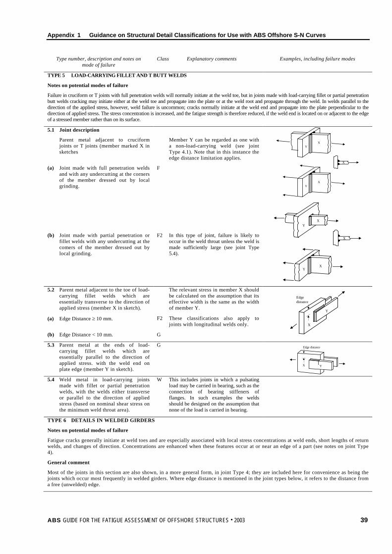
Appendix 1 Guidance on Structural Detail Classifications for Use with ABS Offshore S-N Curves
Type number, description and notes on mode of failure
Class Explanatory comments Examples, including failure modes
TYPE 5 LOAD-CARRYING FILLET AND T BUTT WELDS
Notes on potential modes of failure
Failure in cruciform or T joints with full penetration welds will normally initiate at the weld toe, but in joints made with load-carrying fillet or partial penetration butt welds cracking may initiate either at the weld toe and propagate into the plate or at the weld root and propagate through the weld. In welds parallel to the direction of the applied stress, however, weld failure is uncommon; cracks normally initiate at the weld end and propagate into the plate perpendicular to the direction of applied stress. The stress concentration is increased, and the fatigue strength is therefore reduced, if the weld end is located on or adjacent to the edge of a stressed member rather than on its surface.
5.1 Joint description
XY
XY
X
Parent metal adjacent to cruciform joints or T joints (member marked X in sketches
Member Y can be regarded as one with a non-load-carrying weld (see joint Type 4.1). Note that in this instance the edge distance limitation applies.
(a) Joint made with full penetration welds and with any undercutting at the corners of the member dressed out by local grinding.
F
XY
X
XY
(b) Joint made with partial penetration or fillet welds with any undercutting at the comers of the member dressed out by local grinding.
F2 In this type of joint, failure is likely to occur in the weld throat unless the weld is made sufficiently large (see joint Type 5.4).
5.2 Parent metal adjacent to the toe of load-carrying fillet welds which are essentially transverse to the direction of applied stress (member X in sketch).
The relevant stress in member X should be calculated on the assumption that its effective width is the same as the width of member Y.
X
Y
Edgedistance
(a) Edge Distance ≥ 10 mm. F2 These classifications also apply to joints with longitudinal welds only.
(b) Edge Distance < 10 mm. G
5.3 Parent metal at the ends of load-carrying fillet welds which are essentially parallel to the direction of applied stress. with the weld end on plate edge (member Y in sketch).
G
X Y
Edge distance
5.4 Weld metal in load-carrying joints
made with fillet or partial penetration welds, with the welds either transverse or parallel to the direction of applied stress (based on nominal shear stress on the minimum weld throat area).
W This includes joints in which a pulsating load may be carried in bearing, such as the connection of bearing stiffeners of flanges. In such examples the welds should be designed on the assumption that none of the load is carried in bearing.
TYPE 6 DETAILS IN WELDED GIRDERS
Notes on potential modes of failure
Fatigue cracks generally initiate at weld toes and are especially associated with local stress concentrations at weld ends, short lengths of return welds, and changes of direction. Concentrations are enhanced when these features occur at or near an edge of a part (see notes on joint Type 4).
General comment
Most of the joints in this section are also shown, in a more general form, in joint Type 4; they are included here for convenience as being the joints which occur most frequently in welded girders. Where edge distance is mentioned in the joint types below, it refers to the distance from a free (unwelded) edge.
ABS GUIDE FOR THE FATIGUE ASSESSMENT OF OFFSHORE STRUCTURES . 2003 39

Appendix 1 Guidance on Structural Detail Classifications for Use with ABS Offshore S-N Curves
Type number, description and notes on mode of failure
Class Explanatory comments Examples, including failure modes
6.1 Parent metal at the toe of a weld connecting a stiffener, diaphragm, etc. to a girder flange.
Edge distance refers to distance from a free, i.e. unwelded, edge. In this example, therefore, it is not relevant as far as the (welded) edge of the
Edgedistance
(a) Edge distance ≥ 10mm (see joint Type 4.2).
F Web plate is concerned. For reason for edge distance see note on joint
(b) Edge Distance < 10 mm. G Type 2.
6.2 Parent metal at the end of a weld connecting a stiffener, diaphragm, etc. to a girder web in a region of combined bending and shear.
E This classification includes all attachments to girder webs.
6.3 Parent metal adjacent to welded shear connectors.
Edge distance
(a) Edge distance ≥ 10mm. F
(b) Edge distance < 10mm (see Type 4.2). G
6.4 Parent metal at the end of a partial length welded cover plate, regardless of whether the plate has square or tapered ends and whether or not there are welds across the ends.
G This Class includes cover plates which are wider than the flange. However, such a detail is not recommended because it will almost inevitably result in undercutting of the flange edge where the transverse weld crosses it, as well as involving a longitudinal weld terminating on the flange edge and causing a high stress concentration.
6.5 Parent metal adjacent to the ends of discontinuous welds, e.g. intermittent web/flange welds, tack welds unless subsequently buried in continuous runs.
E This also includes tack welds which are not subsequently buried in a continuous weld. This may be particularly relevant in tack welded backing strips. Note that the existence of the cope hole is allowed for in the joint classification
Ditto. Adjacent to cope holes. F It should not be regarded as an additional stress concentration.
TYPE 7 DETAILS RELATING TO TUBULAR MEMBERS
7.1 Parent material adjacent to the toes of full penetration welded nodal joints.
T In this situation, design should be based on the hot spot stress as defined in Section 3 of this Guide.
7.2 Parent metal at the toes of welds associated with small (≤ 150 mm in the direction parallel to the applied stress) attachments to the tubular member.
F
Ditto, but with attachment length > 150 mm.
F2
40 ABS GUIDE FOR THE FATIGUE ASSESSMENT OF OFFSHORE STRUCTURES . 2003

Appendix 1 Guidance on Structural Detail Classifications for Use with ABS Offshore S-N Curves
ABS GUIDE FOR THE FATIGUE ASSESSMENT OF OFFSHORE STRUCTURES . 2003 41
Type number, description and notes on mode of failure
Class Explanatory comments Examples, including failure modes
7.3 Gusseted connections made with full penetration or fillet welds. (But note that full penetration welds are normally required).
F Note that the design stress must include any local bending stress adjacent to the weld end.
W For failure in the weld throat of fillet welded joints.
7.4 Parent material at the toe of a weld attaching a diaphragm or stiffener to a tubular member.
F Stress should include the stress concentration factor due to overall shape of adjoining structure.
7.5 Parent material adjacent to the toes of circumferential butt welds between tubes.
In this type of joint the stress should include the stress concentration factor to allow for any thickness change and for fabrication tolerances.
(a) Weld made from both sides with the weld overfill dressed flush with the surface and with the weld proved free from significant defects by non-destructive examination.
C The significance of defects should be determined with the aid of specialist advice and/or by the use of fracture mechanics analysis. The NDT technique should be selected with a view to ensuring the detection of such significant defects.
(b) Weld made from both sides. E
(c) Weld made from one side on a permanent backing strip.
F
(d) Weld made from one side without a backing strip provided that full penetration is achieved.
F2 Note that step changes in thickness are in general, not permitted under fatigue conditions, but that where the thickness of the thicker member is not greater than 1.15 × the thickness of the thinner member, the change can be accommodated in the weld profile without any machining.
7.6 Parent material at the toes of circumferential butt welds between tubular and conical sections.
C Class and stress should be those E corresponding to the joint type as F indicated in 7.5, but the stress must also F2 include the stress concentration factor due
to overall form of the joint.
7.7 Parent material (of the stressed member) adjacent to the toes of bevel butt or fillet welded attachments in a region of stress concentration
F Class depends on attachment length or (see Type 4.1) but stress should include F2 the stress concentration factor due to the
overall shape of adjoining structure.
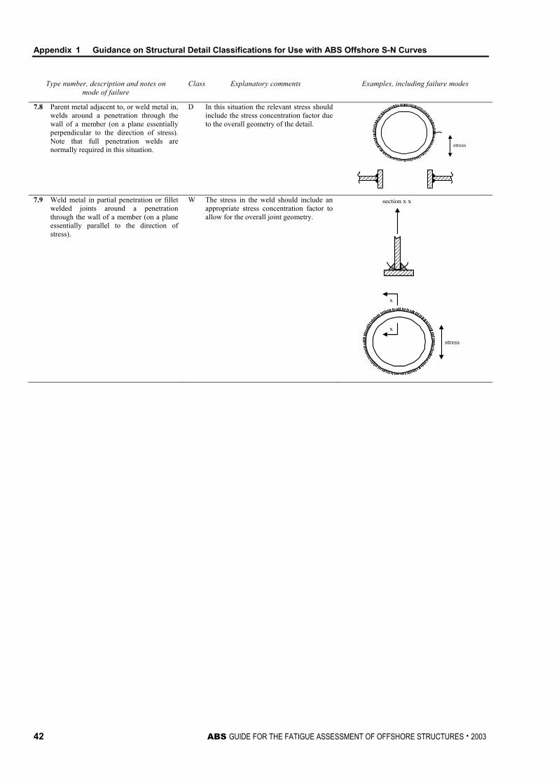
Appendix 1 Guidance on Structural Detail Classifications for Use with ABS Offshore S-N Curves
42 ABS GUIDE FOR THE FATIGUE ASSESSMENT OF OFFSHORE STRUCTURES . 2003
Type number, description and notes on mode of failure
Class Explanatory comments Examples, including failure modes
7.8 Parent metal adjacent to, or weld metal in, welds around a penetration through the wall of a member (on a plane essentially perpendicular to the direction of stress). Note that full penetration welds are normally required in this situation.
D In this situation the relevant stress should include the stress concentration factor due to the overall geometry of the detail.
stress
7.9 Weld metal in partial penetration or fillet welded joints around a penetration through the wall of a member (on a plane essentially parallel to the direction of stress).
W The stress in the weld should include an appropriate stress concentration factor to allow for the overall joint geometry.
x
x
stress
section x x
Appendix 2: References on Parametric Equations for the SCFs of Tubular Intersection Joints
A P P E N D I X 2 References on Parametric Equations for the SCFs of Tubular Intersection Joints*
Several parametric formulae have been produced for the prediction of SCFs for tubular joints, based on data from both physical and FE models.
Simple Joints Appendix 2, Table 1 indicates acceptable formulae for the prediction of SCFs for simple joints. These have been validated against data from large scale steel models and also checked against data from acrylic models and have been shown to provide acceptable predictions.
Multi Planar Joints For multi planar joints SCFs are usually determined assuming there is no interaction between joints in different planes. However, in certain load cases, significant interaction can occur between joints in different planes. These effects, which can result in significantly different SCFs, should be assessed using appropriate methods (e.g., expressions used in Efthymiou 1988).
Overlapped Joints Parametric formulae for the prediction of SCFs in overlapped joints have been published (Efthymiou 1988). They have not been validated because of the limited database available.
Stiffened Joints Parametric SCF formulae for ring-stiffened joints have been developed from acrylic model test data (Smedley and Fisher 1990), which give the brace/chord intersection SCFs in terms of the equivalent, unstiffened joint SCFS. Equations to predict the SCF at the ring inner edge have also been given (Smedley and Fisher 1990).
* The contents of Appendix 2 have been adapted from publications of the U.K. Health and Safety Executive. Permission from the Health and Safety Executive to use the source material is gratefully acknowledged.
ABS GUIDE FOR THE FATIGUE ASSESSMENT OF OFFSHORE STRUCTURES . 2003 43

Appendix 2 References on Parametric Equations for the SCFs of Tubular Intersection Joints
TABLE 1 SCF Matrix Tables for X, K and T/Y Joints
X Joints
Loading Position Efthy S&F
Balanced Axial
Chord Saddle Y X Chord Crown X* X* Brace Saddle Y Y Brace Crown Y Y
Balanced O.P.B Chordside Y Y Braceside Y Y
Balanced I.P.B Chordside Y Y Braceside Y Y
K Joints
Loading Position Efthy S&F
Balanced Axial Chordside X Y Braceside X Y
Unbalanced O.P.B Chordside Y Y Braceside Y Y
Balanced I.P.B Chordside Y Y Braceside YC Y
T/Y Joints
Loading Position Efthy S&F
Axial
Chord Saddle Y Y Chord Crown Y Y Brace Saddle Y Y Brace Crown YC Y
O.P.B Chordside Y Y Braceside Y Y
I.P.B Chordside Y Y Braceside Y X
44 ABS GUIDE FOR THE FATIGUE ASSESSMENT OF OFFSHORE STRUCTURES . 2003

Appendix 2 References on Parametric Equations for the SCFs of Tubular Intersection Joints
Key to A2/Table 1 Y Recommend the equation
YC Recommend the equation – but note that the equation is generally conservative
X Not recommend the equation, since it fails to meet the acceptance criteria
X* The equation cannot be recommended since there are less than 15 steel and acrylic joints in the SCF database.
Efthy Efthymiou Equations (Efthymiou 1988)
S&F Smedley and Fisher Equations (Smedley and Fisher 1991)
NB For X Joints For the chord crown under axial load, the database is too small to recommend any equation. It is recommended that the chord saddle SCF be applied at all periphery locations unless another appropriate method is established.
References P. Smedley and P. Fisher (1990), ‘A Review of Stress Concentration Factors for Complex Tubular Joints’, Integrity of Offshore Structures Conference, Glasgow
P. Smedley and P. Fisher (1991), ‘Stress Concentration Factors for Simple Tubular Joints’, ISOPE
M. Efthymiou (1988), ‘Development of SCF Formulae and Generalized Influence Functions for Use in Fatigue Analyses’, Proceedings of Offshore Tubular Joints Conference, Surrey [with corrections]
ABS GUIDE FOR THE FATIGUE ASSESSMENT OF OFFSHORE STRUCTURES . 2003 45

Appendix 3: Alternative Fatigue Design Criteria for an Offshore Structure to be Sited on the U.S. Outer Continental Shelf
A P P E N D I X 3 Alternative Fatigue Design Criteria for an Offshore Structure to be Sited on the U.S. Outer Continental Shelf
1 General This Appendix is referred to in Sections 3 and 4. It is provided for the use of clients who are required to apply the fatigue criteria cited by the U.S. Minerals Management Service (MMS) for a steel Offshore Structure. The MMS regulations indicate compliance is required with cited U.S. based practices and codes. For steel Offshore Structures, the main criteria referred to for fatigue are those provided in various Recommended Practice documents issued by the American Petroleum Institute (API); i.e. RP 2A, RP 2T, and RP 2FPS. The API RPs in turn make reference to other U.S. based standards, such as those issued by the American Welding Society (AWS).
Appendix 3, Table 1 presents the FDF values and the applicable S-N curves for various types of: offshore structures, structural details, detail locations and other considerations. The ‘Notes for Table 1’, listed after the table, must be observed when using the table.
46 ABS GUIDE FOR THE FATIGUE ASSESSMENT OF OFFSHORE STRUCTURES . 2003

Appendix 3 Alternative Fatigue Design Criteria for an Offshore Structure to be Sited on the U.S. Outer
Continental Shelf
TABLE 1 Fatigue Design Factors for Structural Details**
** The minimum Factor to be applied to uninspectable ‘ordinary’ or uninspectable ‘critical’ structural details is 5 or 10, respectively.
STRUCTURAL DETAIL (3) GOVERNING FATIGUE STRENGTH
CRITERIA
APPLICATION (1) CATEGORY**
LOCATION ORDINARY CRITICAL (2) Structural Subsystem (4) Type
FIXED & FLOATING INSTALLATION ABOVE WATER STRUCTURE Non-Integral Deck (5) Non Tubular (7) AWS (13)
2
3
Tubular Intersection (8)
API
2
3
Integral Deck (6) Non Tubular AWS (13)
3
5
Tubular Intersection
API 3 5
IN WATER & SUBMERGED STRUCTURE (9) Fixed Non-Floating Structure (e.g. fixed jacket, tower and template)
Non Tubular ABS- (CP) (17) 2 3 Tubular Intersection
API
2
3
Fixed Floating Structure (e.g. TLP, Column Stabilized & SPAR; but excluding Ship-type & MODU (15))
Non Tubular (10) ABS- (CP) 3 5 Tubular Intersection
API 3 5
Foundation Components (12) ABS- (CP) or API (for Tubular Intersection Details)
NA NA
10 10
MOORING COMPONENTS (14) ABS FPI Rules (11) NA 3 TLP TENDON (14) See Note 16 NA 10
NOTES for TABLE 1 1 The stated Factors presume that the detail can be inspected at times of anticipated scheduled survey or when structural
damage is suspected. The need to move equipment or covers to provide direct visual access or to employ inspection tools does not disqualify the detail as being ‘inspectable’. However, where the ability to perform direct visual inspection is not evident from the submitted design documentation, any ‘Inspection Plan’ as required by the applicable Rules is to address how it is intended that the required, effective inspection will be accomplished. The use of uninspectable details should be avoided as far as is practicable.
2 A detail is considered critical if its failure will cause the rapid loss of structural integrity AND this produces an event of unacceptable consequence (e.g. loss of life; pollution; loss of platform; collision damage to another structure, facility, or important natural feature). In this context, ‘rapid’ means that even a very local failure can not be detected, inspected and repaired:
• before the occurrence of a broader, catastrophic structural failure, or
• before steps can be taken to eliminate any potential unacceptable consequence.
The designer is responsible to identify all potentially ‘critical’ structural details and to advise what rationale is being taken if the detail is being categorized as ‘ordinary’ (i.e. a detail that is redundant having a lower failure consequence).
3 ‘Structural Detail’ refers to both welded connections and non-welded details.
4 At an interface connection between structural subsystems, the higher (more demanding) of the two applicable requirements shall apply on both sides of the interface connection.
ABS GUIDE FOR THE FATIGUE ASSESSMENT OF OFFSHORE STRUCTURES . 2003 47
Appendix 3 Alternative Fatigue Design Criteria for an Offshore Structure to be Sited on the U.S. Outer
Continental Shelf
5 ‘Non-Integral Deck Structure’ means the deck is not essential for the structural integrity of the structural subsystem supporting the deck.
6 ‘Integral Deck Structure’ means the deck structure is an essential component of the structural integrity of the overall platform structure [e.g. the deck structure spanning the columns of a TLP or a Column Stabilized type platform.]
7 ‘Non-Tubular’ means both non-tubular details (also called ‘plate details’) and non-intersecting tubular details (e.g. butt joints of tubular members and attachments to tubular members)
8 ‘Tubular Intersection’ refers to the nodal connections of tubular brace (branch) members with a tubular chord member.
9 This region is defined as being from the top of the air-gap down to the seabed and beneath to the bottom of the foundation elements (e.g. pile tips). But, for a non-integral deck and for the purposes of the fatigue assessment only, this region can be defined as being from the ‘deck to jacket (or hull) connection’ down to (and below) the seabed.
10 Internal structural tanks that are used for the (non-permanent) storage of seawater may be designed to the ABS- (A) criteria provided:
• Complete recoating is planned to occur in or before the 10th year of structural life,
• An effective coating system is provided to the entire tank (to be considered effective, there should be appropriate surface preparation prior to coating, appropriate application and monitoring of a 2 coat epoxy coating, or at least an equally effective coating),
• The space is accessible for close-up visual inspection to assess coating condition, and
• Arrangements are provided to perform local coating renewal at weld detail locations.
11 Refer to API RP 2SK concerning the components and criteria to be assessed.
12 The factor listed is applicable to the in-place condition. Other criteria may be considered when assessing the installation condition.
13 AWS Criteria may have limitations regarding available geometry, material thickness and corrosiveness.
14 The appropriate criteria to be used for cast structural components will be specially considered.
15 The fatigue assessment of a MODU (e.g. Column Stabilized and Self Elevating types) typically employs the ABS (A) or (CP) criteria, as applicable, with a Fatigue Design Factor of 1.0 for the structural details required by the MODU Rules to undergo a fatigue assessment.
16 Requires special consideration. For guidance, use may be made of AWS C1 or API X curve for tendon girth welds, but see also note 13 regarding AWS criteria. The acceptability of these AWS and API S-N curves requires very high quality NDT of the welds, and appropriate corrosion protection via coating, cathodic protection or both.
17 In the ‘splash zone’ (see Offshore Installations Rules 3-2-4/5.9.2), the use of the ABS (FC) S-N curves may be required.
48 ABS GUIDE FOR THE FATIGUE ASSESSMENT OF OFFSHORE STRUCTURES . 2003