fat chance - dartmouth collegeprob/prob/new/bestofchance.pdf · fat chance charles m. grinstead ......
TRANSCRIPT

Fat Chance
Charles M. Grinstead
Swarthmore College
J. Laurie Snell
Dartmouth College

2

Chapter 1
Fingerprints
1.1 Introduction
On January 7, 2002, in the case U.S. v. Llera-Plaza, Louis H. Pollack, a federal judgein the United States District Court in Philadelphia, barred any expert testimony onfingerprinting that asserted that a particular print gathered at the scene of a crimeis or is not the print of a particular person. As might be imagined, this decision wasmet with much interest, since it seemed to call into question whether fingerprintingcan be used to help prove the guilt or innocence of an accused person.
In this chapter, we will consider the ways in which fingerprints have been usedby society and show how the current quandary was reached. We will also con-sider what probability and statistics have to say about certain questions concerningfingerprints.
1.2 History of Fingerprinting
It seems that the first use of fingerprints in human society was to give evidence ofauthenticity to certain documents in seventh-century China, although it is possiblethat they were used even earlier than this. Fingerprints were used in a similarway in Japan, Tibet, and India. In Simon Cole’s excellent book on the history offingerprinting, the Persian historian Rashid-eddin is quoted as having declared in1303 that “Experience shows that no two individuals have fingers exactly alike.” 1
This statement is one with which the reader is no doubt familiar. A little thoughtwill show that unless all the fingerprints in the world are observed, it is impossibleto verify this statement. Thus, one might turn to a probability model to helpunderstand how likely it is that this statement is true. We will consider such modelsbelow.
In the Western World, fingerprints were not discussed in any written work until1685, when an illustration of the papillary ridges of a thumb was placed in ananatomy book written by the Dutch scientist Govard Bidloo. A century later, the
1Cole, Simon A., “Suspect Identities: A History of Fingerprinting and Criminal Identification,”Harvard University Press, Cambridge, Massachusetts, 2001, pgs. 60-61.
1
2 CHAPTER 1. FINGERPRINTS
statement that fingerprints are unique appeared in a book by the German anatomistJ. C. A. Mayer.
In 1857, a group of Indian conscripts rebelled against the British. After thisrebellion had been put down, the British government decided that it needed tobe more strict in its enforcements of laws in its colonies. William Herschel, thegrandson of the discoverer of the planet Uranus, was the chief administrator of adistrict in Bengal. Herschel noted that the unrest in his district had given rise to agreat amount of perjury and fraud. For example, it was believed that many peoplewere impersonating deceased officers to collect their pensions. Such impersonationwas hard to prove, since there was no method that could be used to decide whethera person was who he or she claimed to be.
In 1858, Herschel asked a road contractor for a handprint, to deter the contractorfrom trying to contest, at a later date, the authenticity of a certain contract. Afew years subsequent to this, Herschel began using fingerprints. It is interesting tonote that as with the Chinese, the first use of fingerprints was in civil, not criminal,identification.
At about the same time, the British were increasingly concerned about crimein India. One of the main problems was to determine whether a person arrestedand tried for a crime was a habitual offender. Of course, to determine this requiredthat some method be used to identify people who had been convicted of crimes.Presumably, a list would be created by the authorities, and if a person was arrested,this list would be consulted to determine whether the person in question was on thelist or not. In order for such a method to be useful, it would have to possess twoproperties. First, there would have to be a way to store, in written form, enoughinformation about a person so as to uniquely identify that person. Second, the listcontaining this information would have to be in a form that would allow quick andaccurate searches.
Although, in hindsight, it might seem obvious that one should use fingerprintsto help with the formation of such a list, this method was not the first to beused. Instead, a system based on anthropometry was developed. Anthropometryis the study and measurement of the size and proportions of the human body. Itwas naturally thought that once adulthood is reached, the lengths of bones do notchange. In the 1880’s Alphonse Bertillon, a French police official, developed a systemin which eleven different measurements were taken and recorded. In addition tothese measurements, a detailed physical description, including information on suchthings as eyes, ears, hair color, general demeanor, and many other attributes, wasrecorded. Finally, descriptions of any ‘peculiar marks’ were recorded. This systemwas called Bertillonage, and was widely used in Europe, India, and the UnitedStates, as well as other locations, for several decades.
One of the main problems encountered in the use of Bertillonage was inconsis-tency in measurement. Many measurements of each person were taken, and the‘operators,’ as the measurers were called, were trained. Nonetheless, if a criminalsuspect was measured in custody, and the suspect’s measurements were already inthe list, the two sets of measurements might vary enough so that no match wouldbe made.

1.2. HISTORY OF FINGERPRINTING 3
Another problem was the amount of time required to search the list of knownoffenders, in order to determine whether a person in custody had been arrestedbefore. In some places in India, the lists grew to contain many thousands of records.Although these records were certainly stored in a logical way, the variations inmeasurements made it necessary to look at many records that were ‘near’ the placethat the searched-for record should be.
The chief problem at that time with the use of fingerprints for identification wasthat no good classification system had been developed. In this regard, fingerprintswere not thought to be as useful as Bertillonage, since the latter method did in-volve numerical records that could be sorted. In the 1880’s, Henry Faulds, a Britishphysician who was serving in a Tokyo hospital at the time, devised a method forclassifying fingerprints. This method consisted of identifying each major type ofprint with a certain written syllable, followed by other syllables representing differ-ent features in the print. Once a set of syllables for a given print was determined,the set was added to a alphabetical list of stored sets of syllables representing otherprints.
Faulds wrote to Charles Darwin about his ideas, and Darwin forwarded them tohis cousin, Francis Galton. Galton was one of the giants among British scientistsin the late 19th century. His interests included meteorology, statistics, psychology,genetics, and geography. Early in his adulthood, he spent two years exploringsouthwest Africa. He was also a promoter of eugenics; in fact, this word is due toGalton.
Galton became interested in fingerprints for several reasons. He was interestedin the heritability of certain traits, and one such trait that could easily be testedwere fingerprint patterns. He was concerned with ethnology, and sought to comparethe various races. One question that he considered in this vein was whether theproportions of the various types of fingerprints differed among the races. He alsotried to determine whether any other traits were related to fingerprints. Finally, heunderstood the value that such a system would have in helping the police and thecourts identify recidivists.
To carry out such research, it was necessary for him to have access to manyfingerprints. By the early 1890’s, he had amassed a collection of thousands ofprints. This collection contained prints from people belonging to many differentethnic groups. He also collected fingerprints from certain types of people, such ascriminals. He was able to show that fingerprints are partially controlled by heredity.For example, it was found that a peculiarity in a pattern in a fingerprint of a parentmight pass to the same finger of a child, or, with less probability, to another fingerof that child. Nonetheless, it must be stated that his work in this area did not leadto any discoveries of great import.
One of Galton’s most fundamental contributions to the study of fingerprintsconsisted of his publishing of material, much of which was due to William Herschel,that fully established the fact that fingerprint patterns persist over the lifetimeof an individual. Of at least equal importance was his development of a methodto classify fingerprints. His method had the important attribute that it could bequickly searched to determine if it contained a given fingerprint.
4 CHAPTER 1. FINGERPRINTS
Very shortly thereafter, a committee consisting of various high officials in Britishlaw enforcement was formed to compare Bertillonage and the Galton fingerprintmethod, with the goal being to decide which method to adopt (although Bertillonagewas in use in continental Europe, India, and elsewhere, it had not yet been usedin Britain). The committee also considered whether it might be still better to useboth methods at once.
In their deliberations, the committee noted that the taking of fingerprints is amuch easier process than the one that is used by Bertillonage operators. In addition,a fingerprint, if it is properly taken (i.e. if the resulting impression is legible), is atrue and accurate rendition of the patterns on the finger. Both of these statementslead to the conclusion that this method is more accurate than Bertillonage.
Given these remarks, it might seem strange that the committee did not rec-ommend that fingerprints be the method of choice. However, there was still someconcern about the accuracy of the indexing used in the method. It was recom-mended that identification be made by fingerprints, but indexing be carried out byBertillonage. The committee did foresee that the problems with fingerprint index-ing could be overcome, and that in this case, the fingerprint method might be thesole system in use.
Galton continued to work on his method of classification, and in 1895, he pub-lished a system that greatly improved his previous attempts. Edward Henry, amagistrate of a district in India, worked on and modified Galton’s indexing methodbetween 1898 and 1900. This modification was adobted by Scotland Yard. Regard-ing credit for the method, a letter from Sir George Darwin to the London Times hadthis to say: “Sir Edward Henry undoubtedly deserves great credit in recognisingthe merits of the system and in organising its use in a practical manner in India,the Cape and England, but it would seem that the yet greater credit is due to Mr.Francis Galton.”2
In 1902, Galton published a letter in the journal Nature, entitled “Finger-PrintEvidence,” in which he discusses a new aspect (for him, at any rate) of fingerprints.Scotland Yard had sent him two enlarged photographs of thumbprints. The firstcame from the scene of a burglary, and the second came from the fingerprint files atScotland Yard. Galton discusses how the use of his system allows the prosecutionto explain the similarities in the two prints. The question of accuracy in matchingprints obtained from a crime scene with those in a database is one that is still beingconsidered today. Before turning to this question, we will describe Galton’s method.
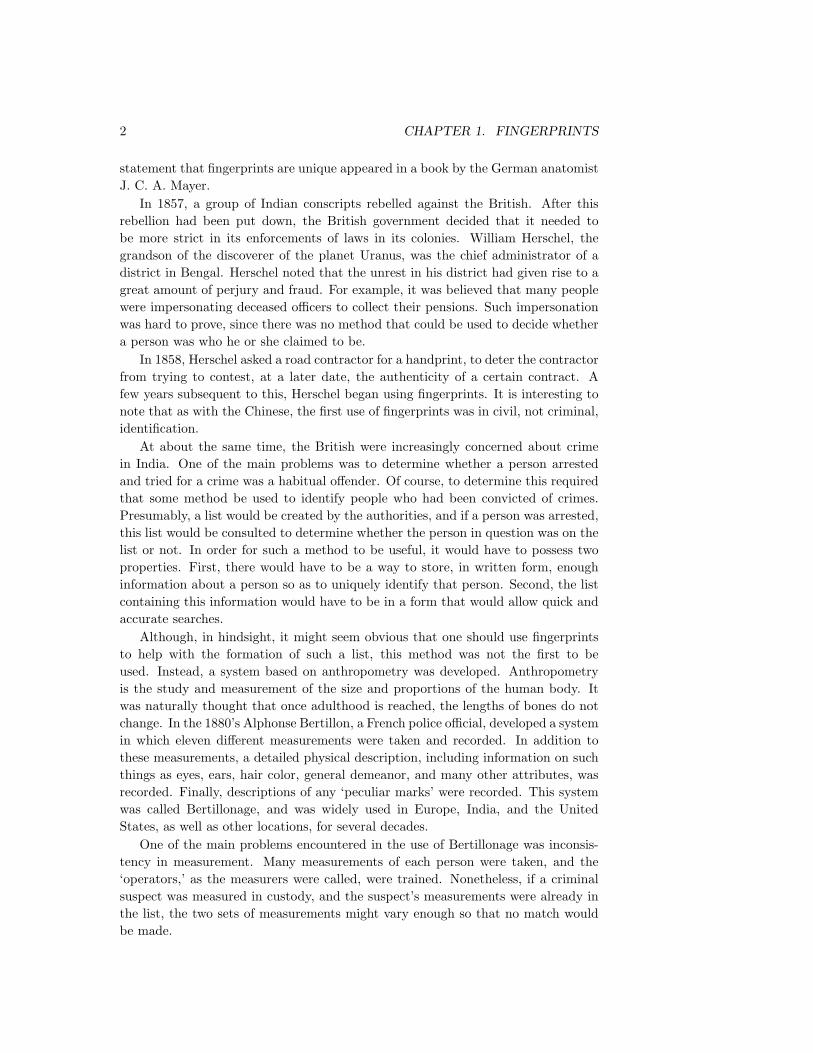
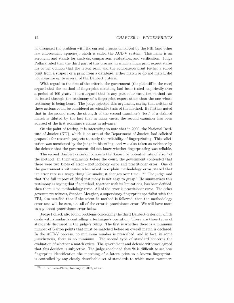
Galton begins by noting that in the center of most fingerprints there is a ‘core,’which consists of patterns that he calls loops and whorls (see Figure 1.13.) If nosuch core exists, the pattern is said to be an arch. Next, he defines a delta as theregion where the parallel ridges begin to diverge to form the core. Loops have onedelta, and whorls have two. These deltas serve as axes of reference for the rest ofthe classification. By tracing the ridges as they leave the delta(s) and cross thecore, one can partition fingerprints into ten classes. Since each finger would be in
2George Darwin, quoted in Karl Pearson, “Life and Letters of Francis Galton,”3Keogh, E.,An Overview of the Science of Fingerprints. Anil Aggrawal’s Internet Journal of
Forensic Medicine and Toxicology, 2001; Vol. 2, No. 1 (January-June 2001)

1.3. MODELS OF FINGERPRINTS 5
Figure 1.1: Four examples of fingerprints.
one of the ten classes, there are 1010 possible sets of ten classes. Even though theten classes do not occur with equal frequency among all fingerprints, this first levelof classification already serves to distinguish between most pairs of people.
Of the ten classes, only two correspond to loops, as opposed to arches andwhorls. However, about half of all fingerprints are loops, which suggests that thescheme is not yet precise enough. Galton was aware of this, and added two othertypes of information to the process. The first involved using the axes of referencearising from the deltas to count ridges in certain directions. The second involvedthe counting and classification of what he termed ‘minutiae.’ This term refers toplaces in the print where a ridge bifurcates or ends. The idea of minutiae is stillin use today, although they are now sometimes referred to as ‘Galton points’ or‘points.’
There are many different types of points, and the places that they occur in agiven fingerprint seems to be somewhat random. In addition, a typical fingerprinthas many such points. These observations imply that if one can accurately writedown where the points occur and which types of points occur, then one has a verypowerful way to distinguish two fingerprints. The method is even more powerfulwhen comparing sets of ten fingerprints from two people.
1.3 Models of Fingerprints
We shall investigate some probabilistic models for fingerprints that incorporate theidea of points. The two most basic questions that one might use such modelsto help answer are as follows. First, in a given model, what is the probabilitythat no two fingerprints, among all people who are now alive, are exactly alike?Second, suppose that we have a partial fingerprint, such as one that might have beenrecovered from a crime scene (such partial prints are called latent prints). Whatis the probability that this latent print exactly matches more than one fingerprint,among all fingerprints in the world? The reason that we are interested in whetherthe latent print matches more than one fingerprint is that it clearly matches oneprint, namely the one belonging to the person who left the latent print. It is typicallythe case that the latent print, if it is to be of any use, will identify a suspect, i.e.
6 CHAPTER 1. FINGERPRINTS
someone who has a fingerprint that matches the latent print. It is obviously of greatinterest in a court of law as to how likely it is that someone other than the suspecthas a fingerprint that matches the latent print. We will see that this second questionis of central importance in the discussions going on today about the accuracy offingerprinting as a crimefighting tool.
Galton seems to have been the first person to consider a probabilistic model thatmight shed some light on the answer to the first question. He began by imagininga fingerprint as a random set of ridges, with roughly 24 ridge intervals across thefinger and 36 ridge intervals along the finger. Next, he imagined covering up an n byn ridge interval square on a fingerprint, and attempting to recreate the ridge patternin the area that was covered. Galton maintained that if n were small, say at most4, then most of the time, the pattern could be recreated by using the informationin the rest of the fingerprint. However, if n were 6, he found that he was wrongmore often than right when he carried out this experiment.
He then let n = 5, and claimed that he would be right about one-half of thetime in reconstructing the fingerprint. This led him to consider the fingerprint asconsisting of a set of non-overlapping n x n squares, which he considered to beindependent random variables. In Pearson’s account, Galton used n = 6, althoughhis argument is more understandable had he used n = 5. Galton claimed that anyof the reconstructions, both the correct and incorrect ones, might have occurredin nature, so each random variable has two possible values,given the way that theridges leave and enter the square, and given how many ridges leave and enter.Pearson says that Galton ‘proceeds to gived a rough approximation to two otherchances, which he considers to be involved: the first concerns guessing correctlythe general course of the ridges adjacent to each square, and the second of guessingrightly the number of ridges that enter and issue from the square. He takes thesein round numbers to be 1/24 and 1/28... .’4 Finally, Galton multiplies all of theseprobabilities together, under the assumption of independence, and arrives at thenumber 64 billion which, at the time, was 4 times the number of fingerprints inthe world. (Galton claims that the odds are roughly 39 to 1 against any particularfingerprint occurring anywhere in the world. It seems to us that the odds shouldbe 3 to 1 against.)
We will soon see other models of fingerprints that arrive at much different an-swers. However, it should be remembered that we are trying to estimate the prob-ability that no two fingerprints, among all people who are now alive, are exactlyalike. Suppose, as Galton did, that there are 16 billion fingerprints among thepeople of the world, and there are 64 billion possible fingerprints. Does the readerthink that these assumptions make it very likely or very unlikely that there are twofingerprints that are the same? To answer this question, we can proceed as follows.Consider an urn with 64 billion labeled balls in it. We choose, one at a time, 16billion balls from the urn, replacing the balls after each choice. We are asking forthe probability that we never choose the same ball more than once. This is thecelebrated birthday problem, on a world where there are 64 billion days in a year,
4Pearson, ibid., pg. 182.

1.3. MODELS OF FINGERPRINTS 7
and 16 billion people. The birthday problem asks what is the probability that atleast two people share a birthday. The answer is(
1− 0n
)(1− 1
n
)(1− 2
n
). . .
(1− k − 1
n
),
where n = 64 billion and k = 16 billion. This can be seen by considering the peopleone at a time. If 6 people, say, have already been considered, and if they all havedifferent birthdays, then the probability that the seventh person has a birthday thatis different than all of the first 6 people equals(
1− 6n
).
It is relatively straightforward to estimate the above product in terms of k and n.For the values given by Galton, the product is less than
110109 .
This means that in Galton’s model, with his estimates, it is extremely likely thatthere are two fingerprints that are the same.
In fact, to our knowledge, no two fingerprints from different people have everbeen found that are identical. Of course, it is not the case that all fingerprintson Earth have been recorded or compared, but the FBI has a database with morethan 10 million fingerprints in it, and we presume that no two fingerprints in itare exactly the same. (It must be said that it is not clear to us that all pairs offingerprints in this database have actually been compared. In addition, one wonderswhether the FBI, if it found a pair of identical fingerprints, would announce thisto the world.) In any case, if we use Galton’s estimate for the number of possiblefingerprints, and let k = 10 million, the probability that no two are alike is stillvery small; it is less than
110339
.
We can turn the above question around and ask the following question. Supposethat there are 60 billion fingerprints in the world, and suppose that we imagine theyare chosen from a set of n possible fingerprints. How large would n have to be inorder that the probability that all of the chosen fingerprints are different exceeds.999? An approximate answer to this question is that it would suffice for n to beat least 1025. Although this is quite a bit larger than Galton’s estimate, there havebeen other, more sophisticated models of fingerprints, some of which we will nowdescribe, have come up with estimates for n that are much larger than 1025. Thus,if these models are at all accurate, it is extremely unlikely that there exist twofingerprints in the world that are exactly alike.
In 1933, T. Roxburgh described a model for fingerprint classification that is muchmore intricate than Galton’s model. This model, and many others, are describedand compared in an article in the Journal of Forensic Sciences, written by D. A.
8 CHAPTER 1. FINGERPRINTS
Stoney and J. I. Thornton.5 In Roxburgh’s model, a vertical ray is drawn upwardsfrom the center of the fingerprint (this idea must be accurately defined, but for ourpurposes, we can take it to mean the center of the loop or whorl, or the top of thearch). This ray is defined to be 0 degrees. Another ray, with endpoint at the center,is revolved clockwise from the first ray. As this ray passes over minutiae, the typesof the minutiae are recorded, along with the ridge numbers on which the minutiaelie. If a fingerprint has R concentric ridges, n minutiae, and there are T minutiatypes, then the number of possible patterns equals
(RT )n ,
since as the second ray revolves clockwise, the next minutia encountered could be onany of the R ridges and be of any of the T minutia types. Roxburgh also introducesa factor of P that corresponds to the number of different overall patterns andcore types that might be encountered. Thus, he estimates the number of possiblefingerprints to be
P (RT )n .
He takes P = 1000, R = 10, T = 4, and n = 35; this last value is Galton’sestimate for the typical number of minutia in a fingerprint. If we calculate theabove expression with these values, we obtain the number
1.18× 1059 .
Roxburgh modified the above expression for the number of possible fingerprintsto attempt to account for ambiguities between various types of minutiae. For exam-ple, it is possible that a fork in a ridge might be seen as a ridge ending, dependingupon whether the ridges in question meet each other or not. Roxburgh suggestedusing a number Q which would vary depending upon the quality of the fingerprintunder examination. The value of Q ranges from 1.5 to 3, with the smaller valuecorresponding to a higher quality fingerprint. For each minutia, Roxburgh replacedthe factor RT by the factor RT/Q. This leads to the expression
P ((RT )/Q)n
as an estimate for the number of discernable types of fingerprints, assuming theirquality corresponds to a particular value of Q. Note that even if Q = 3, so thatRT/Q = 1.33R, the number of discernable types of fingerprints in this model is
2.16× 1042 .
Stoney and Thornton note that although this is a very interesting, sophisticatedmodel, it has been “totally ignored by the forensic science community.”6
5Stoney, D. A. and J. I. Thornton, “A Critical Analysis of Quantitative Fingerprint Individu-ality Models,” Journal of Forensic Sciences, v. 31, no. 4 (1986), pgs. 1187-1216.
6ibid., pg. 1192

1.4. LATENT FINGERPRINTS 9
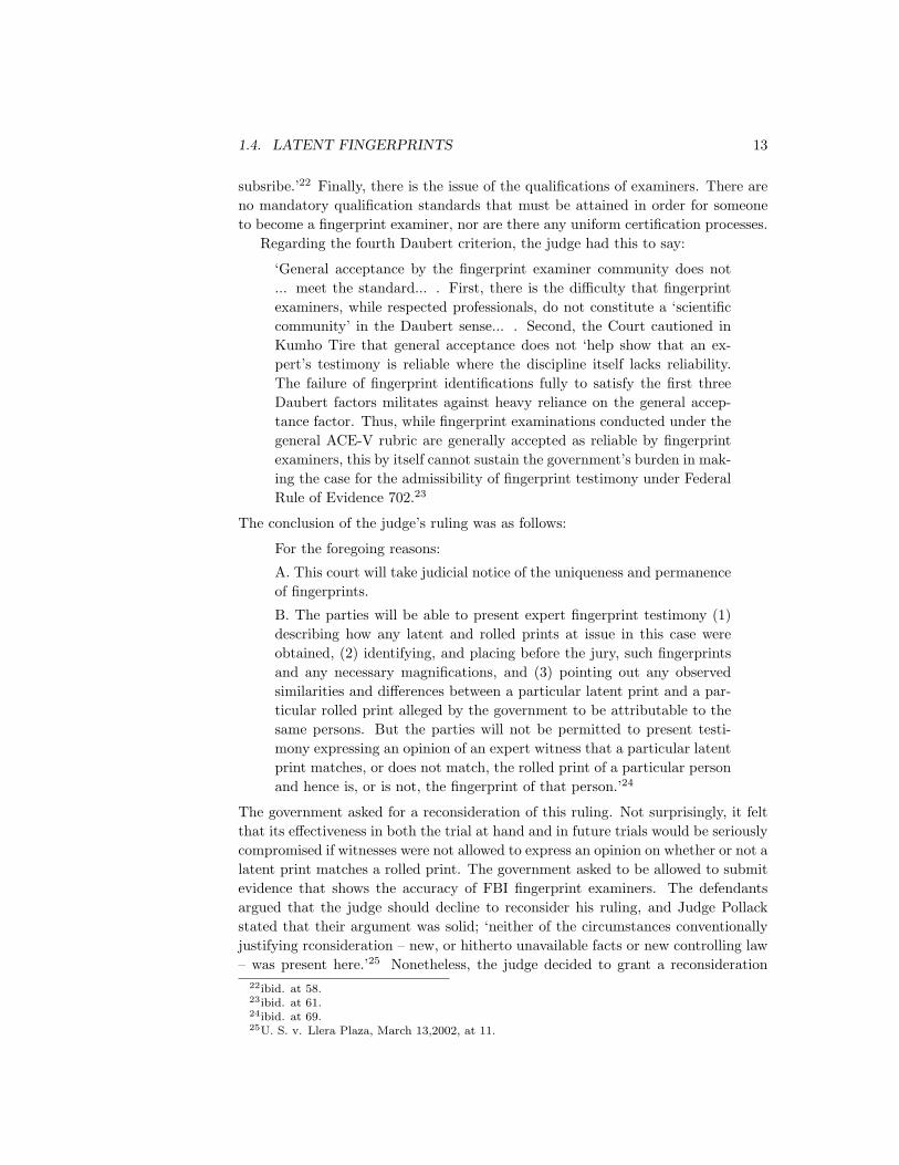
Figure 1.2: Examples of latent and rolled prints.
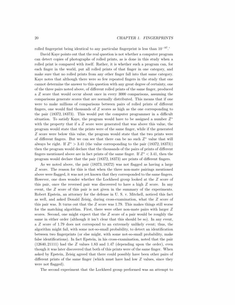
Figure 1.3: Minutiae matches.
1.4 Latent Fingerprints
According to a government expert who testified at a recent trial, the average size ofa latent fingerprint fragment is about one-fifth the size of a full fingerprint. Sincea typical fingerprint contains between 75 and 175 minutiae7, this means that atypical latent print has between 15 and 35 minutiae. In addition, the latent printrecovered from a crime scene is frequently of poor quality, which tends to increasethe likelihood of mistaking the types of minutiae being observed.
In a criminal case, the latent print is compared with a high quality print takenfrom the hand of the accused or from a database of fingerprints. Figure 1.2 showsa latent print and the corresponding rolled print to which the latent print wasmatched. Figure 1.3 shows another pair of prints, one latent and one rolled, fromthe same case. The figure also shows the claimed matching minutiae in the twoprints.
The person making the comparison states that there is a match if he or shebelieves that there are a sufficient number of common minutiae, both in type and
7‘An Analysis of Standards in Fingerprint Identification 1,’ Federal Bureau of Investigation,Department of Justice, Law Enforcement Bulletin, vol. 1 (June 1972).

10 CHAPTER 1. FINGERPRINTS
location, in the two prints. There have been many criminal cases in which an iden-tification was made with fewer than fifteen matching minutiae8. There is no generalagreement among various law enforcement agencies or among various countries, onthe number of matching minutiae that must exist in order for a match to be de-clared. In fact, according to Robert Epstein9, “many examiners ... including thoseat the FBI, currently believe that there should be no minimum standard whatsoeverand that the determination of whether there is a sufficient basis for an identificationshould be left to the subjective judgment of the individual examiner.” It is quiteunderstandable that a law enforcement agency might object to constraints on itsability to claim matches between fingerprints, as this could only serve to decreasethe number of matches obtained.
In some countries, fingerprint matches can be declared with as few as eightminutiae matches (such minutiae matches are sometimes called ‘points.’) However,there are examples of fingerprints from different people that have seven matchingminutiae. In a California bank robbery trial, U. S. v. Parks, in 1991, the prosecutionintroduced evidence that showed that the suspect’s fingerprint and the latent printhad ten points. The trial judge, Spencer Letts, asked the prosecution expert whatthe minimum standard was for points in order to declare a match. The expertannounced that the minimum was eight. Judge Letts had seen fingerprint evidenceentered in other trials. He said “If you only have ten points, you’re comfortablewith eight; if you have twelve, you’re comfortable with ten; if you have fifty, you’recomfortable with twenty.”10 Later in the same trial, the following exchange occurredbetween Judge Letts and another prosecution fingerprint expert:
“The Witness: ‘The thing you have there is that each department has their owngoals or their own rules as far as the number of points being a make [an identifica-tion]. ...that number really just varies from department to department.’
The Court: ‘I don’t think I’m ever going to use fingerprint testimony again; thatsimply won’t do...’
The Witness: ‘That just may be one of the problems of the field, but I think ifthere was [a] survey taken, you would probably get a different number from everydepartment that has a fingerprint section as to their lowest number of points for acomparison and make.’
The Court: ‘That’s the most incredible thing I’ve ever heard of.’ ”11
According to Simon Cole, no scientific study has been carried out to estimate theprobability of two different prints sharing a given number of minutiae. David Stoneyand John Thornton claim that none of the fingerprint models proposed during thepast century “even approaches theoretical accuracy ..., and none has been subjectedto empirical validations.”12 In fact, latent print examiners are prohibited by their
8see footnote 25 in Epstein, Robert, ‘Fingerprints Meet Daubert: The Myth of Fingerprint“Science” is Revealed,’ Southern California Law Review, vol. 75 (2002), pgs. 605-658.
9ibid., pg. 61010Cole, op. cit., pg. 272.11ibid., pgs 272-273.12Stoney and Thornton, op. cit., pg. 1187.

1.4. LATENT FINGERPRINTS 11
primary professional association, the International Association for Identification(“IAI”), from offering opinions of identification using probabilistic terminology. Aresolution, passed by the IAI at one of its meetings, states that “any member,officer, or certified latent print examiner who provides oral or written reports, orgives testimony of possible, probable, or likely friction ridge identification shall bedeemed to be engaged in [unbecoming] conduct... and charges may be brought.”13
In 1993, the Supreme Court rendered a decision in the case Daubert v. Mer-rell Dow Pharmaceuticals, Inc.14 The Court described certain factors that courtsneeded to consider when deciding whether to admit expert testimony. In this de-cision, the Court concentrated on scientific expert testimony; it considered theissue of expert testimony of a non-scientific nature in the case Kumho Tire Co. v.Carmichael, a few years later.15 In the first decision, the Court interpreted the Fed-eral Rule of Evidence 702, which defines the term ‘expert witness’ and states whensuch witness are allowed, as requiring trial judges to determine whether the opinionof an expert witness lacks sufficient reliability, and if so, to exclude this testimony.The Daubert decision listed five factors that could be considered when determiningwhether scientific expert testimony should be retained or excluded. These factorsare as follows:
1. “A preliminary assessment of whether the reasoning or methodology underlyingthe testimony is scientifically valid and of whether that reasoning or methodologyproperly can be applied to the facts in issue.”16
2. “The court ordinarily should consider the known or potential rate of error... .”17
3. The court should consider “the existence and maintenance of standards control-ling the technique’s operation... .”18
4. “‘General acceptance’ can ... have a bearing on the inquiry. A ”reliabilityassessment does not require, although it does permit, explicit identification of arelevant scientific community and an express determination of a particular degreeof acceptance within that community.”’19
5. “A pertinent consideration is whether the theory or technique has been subjectedto peer review and publication... .”20
In the Kumho case, the Court held that a trial court’s obligation to decidewhether to admit expert testimony applies to all experts, not just scientific experts.The Court also held that the factors listed above may be used by a court in assessingnonscientific expert testimony.
In the case (U.S. v. Llera-Plaza) mentioned at the beginning of the chapter,the presiding judge, Louis Pollack, applied the Daubert criteria to the fingerprintidentification process, as he was instructed to do by the Kumho case. In particular,
13Epstein, op. cit., pg. 611, footnote 32.14509 U.S. 579 (1993)15526 U.S. 137 (1999).16509 U.S. 579 (1993), note 593.17ibid., note 59418ibid.19ibid., quoted from United States v. Downing, 753 F.2d 1224, 1238 (3d Cir. 1985).20ibid., note 593.
12 CHAPTER 1. FINGERPRINTS
he discussed the problem with the current process employed by the FBI (and otherlaw enforcement agencies), which is called the ACE-V system. This name is anacronym, and stands for analysis, comparison, evaluation, and verification. JudgePollack ruled that the third part of this process, in which a fingerprint expert stateshis or her opinion that the latent print and the comparison print (either a rolledprint from a suspect or a print from a database) either match or do not match, didnot measure up to several of the Daubert criteria.
With regard to the first of the criteria, the government (the plaintiff in the case)argued that the method of fingerprint matching had been tested empirically overa period of 100 years. It also argued that in any particular case, the method canbe tested through the testimony of a fingerprint expert other than the one whosetestimony is being heard. The judge rejected this argument, saying that neither ofthese actions could be considered as scientific tests of the method. He further notedthat in the second case, the strength of the second examiner’s ‘test’ of a claimedmatch is diluted by the fact that in many cases, the second examiner has beenadvised of the first examiner’s claims in advance.
On the point of testing, it is interesting to note that in 2000, the National Insti-tute of Justice (NIJ), which is an arm of the Department of Justice, had solicitedproposals for research projects to study the reliability of fingerprinting. This solici-tation was mentioned by the judge in his ruling, and was also taken as evidence bythe defense that the government did not know whether fingerprinting was reliable.
The second Daubert criterion concerns the ‘known or potential rate of error’ ofthe method. In their arguments before the court, the government contended thatthere were two types of error - methodology error and practitioner error. One ofthe government’s witnesses, when asked to explain methodology error, stated that‘an error rate is a wispy thing like smoke, it changes over time...’21 The judge saidthat ‘the full import of [this] testimony is not easy to grasp.’ He summarizes thistestimony as saying that if a method, together with its limitations, has been defined,then there is no methodology error. All of the error is practitioner error. The othergovernment witness, Stephen Meagher, a supervisory fingerprint specialist with theFBI, also testified that if the scientific method is followed, then the methodologyerror rate will be zero, i.e. all of the error is practitioner error. We will have moreto say about practitioner error below.
Judge Pollack also found problems concerning the third Daubert criterion, whichdeals with standards controlling a technique’s operation. There are three types ofstandards discussed in the judge’s ruling. The first is whether there is a minimumnumber of Galton points that must be matched before an overall match is declared.In the ACE-V process, no minimum number is prescribed, and in fact, in somejurisdictions, there is no minimum. The second type of standard concerns theevaluation of whether a match exists. The government and defense witnesses agreedthat this decision is subjective. The judge concluded that ‘it is difficult to see howfingerprint identification–the matching of a latent print to a known fingerprint–is controlled by any clearly describable set of standards to which most examiners
21U.S. v. Llera-Plaza, January 7, 2002, at 47.
1.4. LATENT FINGERPRINTS 13
subsribe.’22 Finally, there is the issue of the qualifications of examiners. There areno mandatory qualification standards that must be attained in order for someoneto become a fingerprint examiner, nor are there any uniform certification processes.
Regarding the fourth Daubert criterion, the judge had this to say:
‘General acceptance by the fingerprint examiner community does not... meet the standard... . First, there is the difficulty that fingerprintexaminers, while respected professionals, do not constitute a ‘scientificcommunity’ in the Daubert sense... . Second, the Court cautioned inKumho Tire that general acceptance does not ‘help show that an ex-pert’s testimony is reliable where the discipline itself lacks reliability.The failure of fingerprint identifications fully to satisfy the first threeDaubert factors militates against heavy reliance on the general accep-tance factor. Thus, while fingerprint examinations conducted under thegeneral ACE-V rubric are generally accepted as reliable by fingerprintexaminers, this by itself cannot sustain the government’s burden in mak-ing the case for the admissibility of fingerprint testimony under FederalRule of Evidence 702.23
The conclusion of the judge’s ruling was as follows:
For the foregoing reasons:
A. This court will take judicial notice of the uniqueness and permanenceof fingerprints.
B. The parties will be able to present expert fingerprint testimony (1)describing how any latent and rolled prints at issue in this case wereobtained, (2) identifying, and placing before the jury, such fingerprintsand any necessary magnifications, and (3) pointing out any observedsimilarities and differences between a particular latent print and a par-ticular rolled print alleged by the government to be attributable to thesame persons. But the parties will not be permitted to present testi-mony expressing an opinion of an expert witness that a particular latentprint matches, or does not match, the rolled print of a particular personand hence is, or is not, the fingerprint of that person.’24
The government asked for a reconsideration of this ruling. Not surprisingly, it feltthat its effectiveness in both the trial at hand and in future trials would be seriouslycompromised if witnesses were not allowed to express an opinion on whether or not alatent print matches a rolled print. The government asked to be allowed to submitevidence that shows the accuracy of FBI fingerprint examiners. The defendantsargued that the judge should decline to reconsider his ruling, and Judge Pollackstated that their argument was solid; ‘neither of the circumstances conventionallyjustifying rconsideration – new, or hitherto unavailable facts or new controlling law– was present here.’25 Nonetheless, the judge decided to grant a reconsideration
22ibid. at 58.23ibid. at 61.24ibid. at 69.25U. S. v. Llera Plaza, March 13,2002, at 11.

14 CHAPTER 1. FINGERPRINTS
hearing, arguing that the record on which he made his previous ruling was testimonypresented two years earlier in another courtroom. ‘It seemed prudent to hear suchlive witnesses as the government wished to present, together with any rebuttalwitnesses the defense would elect to present.’26
At this point in our narrative, it makes sense to consider the various attemptsto measure error rates in the field of fingerprint analysis. Lyn and Ralph Haber,who are consultants at a private company in California, and are also adjuncts atthe University of California at Santa Cruz, have obtained and analyzed relevantdata from many sources.27 These data include both results on crime laboratoriesand individual practitioners. We will summarize some of their findings here.
The American Society of Crime Laboratory Directors (ASCLD) is an organiza-tion that provides leadership in the management of forensic science. It is in theirinterest to evaluate and improve the quality of operations of crime laboratories. In1977, the ASCLD began developing an accreditation program for crime laboratories.By 1999, 182 labs had been accredited. One requirement for a lab to be accreditedis that the examiners working in the lab must pass an externally administered pro-ficiency test. We note that since it is the lab, and not the individual examiners,that is being tested, these proficiency tests are taken by all of the examiners as agroup in a given lab.
Beginning in 1983, the ASCLD began administering such a test in the area offingerprint identification. The test, which is given each year to all labs requestingaccreditation, consists of pictures of 12 or more latent prints and a set of ten-print(rolled print) cards. The set of latent prints contains a range of quality, and issupposed to be representative of what is actually seen in practice. For each latentprint, the lab was asked to decide whether it is ‘scorable,’ i.e. whether it is ofsufficient quality to attempt to match it with a rolled print. If it is judged to bescorable, then the lab is asked to decide whether or not it matches one of the printson the ten-print cards. There are ‘correct’ answers for each latent print on the test,i.e. the ASCLD has decided, in each case, whether or not a latent print is scorable,and if so, whether or not it matches any of the rolled prints.
The Habers report on results from 1983 to 1991. During this time, the numberof labs that took the exam increased from 24 to 88; many labs took the tests morethan once (a new test was constructed each year). Assuming that in many cases,the labs have more than one fingerprint expert, this means that hundreds of theseexperts took this test at least once during this period.
Each lab returned one answer for each question. There are four types of errorthat can be made on each question of each test. A scorable print can be ruledunscorable, or vice versa. If a print is scorable, it can be erroneously matched toa rolled print, or it can fail to be matched at all, even though a match exists. Ofthese four types of errors, the second and third are more serious than the others,assuming that we take the point of view that erroneous evidence against an innocent
26ibid.27Haber, Lynn, and Ralph Norman Haber, “Error Rates for Human Latent Fingerprint Ex-
aminers,” in Advances in Automatic Fingerprint Recognition, Nalini K. Ratha, ed., New York,Springer-Verlag, 2003.

1.4. LATENT FINGERPRINTS 15
person should be strenuously guarded against.The percentage of answers with errors of each of the four types were 8%, 2%,
2%, and 8%, respectively. What should we make of these error rates? We seethat the more serious types of errors had lower rates, but we must remember thatthese answers are consensus answers of the experts in a given lab. For purposes ofillustration, suppose that there are two experts in a given lab, and they agree onan answer that turns out to be incorrect. Presumably they consulted each otheron their answers, so we cannot multiply their individual error rates to obtain theirgroup error rate, since their answers were not independent events. However, we cancertainly say that if the lab error rate is 2%, say, then the individual error rates ofthe experts at the lab who took the test are all at least 2%.
In 1994, the ASCLD asked the IAI for assistance in creating and reviewingfuture tests. The IAI asked a company called Collaborative Testing Services (CTS)to design and administer these tests. The format of these tests is similar to theearlier ones, but all of the latent prints are scorable, so there are only two possibletypes of errors for each question. In addition, individual fingerprint examiners whowish to do so may take the exam by themselves. The Habers report on the errorrates for the examinations given from 1995 through 2001. Of the 1685 tests thatwere graded by CTS, 95 of them, or more than 5%, had at least one erroneousidentification, and 502 of the tests, or more than 29%, had at least one missedidentification.
Since 1995, the FBI has administered its own examinations to all of its fingerprintexaminers. These examinations are similar in nature to the ones described above,but there are a few differences worthy of note. These differences were described inJudge Pollack’s reconsideration ruling, in the testimony of Allan Bayle, a fingerprintexaminer for 25 years at Scotland Yard.28
Mr. Bayle had reviewed copies of the internal FBI proficiency testsbefore taking the stand. He found the latent prints utilized in thosetests to be, on the whole, markedly unrepresentative of the latent printsthat would be lifted at a crime scene. In general, Mr. Bayle found thetest latent prints to be far clearer than the prints an examiner wouldroutinely deal with. The prints were too clear – they were, accordingto Mr. Bayle, lacking in the ‘background noise’ and ‘distortion’ onewould expect in latent prints that were not identifyable; according toMr. Bayle, at a typical crime scene only about ten per cent of the liftedlatent prints will turn out to be matched. In Mr. Bayle’s view thepaucity of non-identifyable prints: ‘makes the test too easy. It’s nottesting their ability. It doesn’t test their expertise. I mean I’ve set thesetests to trainees and advanced technicians. And if I gave my expertsthese tests, they’d fall about laughing.’
Approximately 60 FBI fingerprint examiners took the FBI test each year in theperiod from 1995 to 2001. On these tests, virtually all of the latent prints hadmatches among the rolled prints. Since many of the examiners took the tests most
28U. S. v. Llera Plaza, March 13,2002, at 24.

16 CHAPTER 1. FINGERPRINTS
or all of these years, it is reasonable to suppose that they knew this fact, and hencewould hardly ever claim that a latent print had no match. The results of thesetests are as follows: there were no erroneous matches, and only three cases wherean examiner claimed there was no match when there was one. Thus, the error ratesfor the two types of error were 0% and 1%.
It seems clear that the error rates of the crime labs for the various types of errorare small, but not negligible, and the FBI’s rates are suspect for the reasons givenabove. Given that in many criminal cases, fingerprint evidence forms a crucial partof the prosecution’s case, it is reasonable to ask whether the above data, were it tobe submitted to a jury, would make it difficult for the jury to find the defendantguilty ‘beyond a reasonable doubt,’ which is the standard that must be met in suchcases.
The question of what this last phrase means is a fascinating one. The U.S.Supreme Court recently weighed in on this issue, and the majority opinion is thor-ough in its attempt to explicate the history of the usage of this phrase. The Courtagreed to review two cases involving instructions given to juries by judges. Standardinstructions to juries state that ‘guilt beyond a reasonable doubt’ means that the ju-rors need to be convinced ‘to a moral certainty’ of the defendant’s guilt. In one case,‘California defended the use of the moral-certainty language as a ‘commonsense andnatural’ phrase that conveys an ‘extraordinarily high degree of certainty.’29 In thesecond case, a judge in Nebraska ‘included not only the moral-certainty languagebut also a definition of reasonable doubt as ’an actual and substantial doubt.’ Thejurors were instructed that ’you may find an accused guilty upon the strong prob-abilities of the case, provided such probabilities are strong enough to exclude anydoubt of his guilt that is reasonable.’30 The Supreme Court upheld both sets of in-structions. The decision regarding the first set was unanimous, while in the secondcase, two justices dissented, noting that ‘the jury was likely to have interpreted thephrase ‘substantial doubt’ to mean that ‘a large as opposed to a merely reasonabledoubt is required to acquit a defendant.”31
The Court went on to note that the meaning of the phrase ‘moral certainty’has changed over time. In the mid-19th century, the phrase generally meant a highdegree of certainty, whereas today, some dictionaries define the phrase to mean‘based on strong likelihood or firm conviction, rather than on the actual evidence.’32
Although the Court upheld both sets of instructions, the majority opinion statedthat the Court did not condone the use of the phrase ‘moral certainty.’
In a concurring opinion, Justice Ruth Bader Ginsburg noted that some Federalappellate circuit courts have instructed trial judges not to provide any definitionof the phrase ‘beyond a reasonable doubt.’ Justice Ginsburg said that it would bebetter to construct a better definition than the one used in the instructions in thecases under review. She ‘cited one suggested in 1987 by the Federal Judicial Center,a research arm of the Federal judiciary. Making no reference to moral certainty, that
29Linda Greenhouse, ‘High Court Warns About Test for Reasonable Doubt,’ The New YorkTimes, March 22, 1994
30ibid.31ibid.32American Heritage Dictionary of the English Language, 1992.

1.5. THE 50K STUDY 17
definition says in part, ‘Proof beyond a reasonable doubt is proof that leaves youfirmly convinced of the defendant’s guilt.”33
It may very well be the case that after wading through the above verbiage, thereader has no clearer an idea (and perhaps even has a less clear idea) than beforeof what the phrase ‘beyond a reasonable doubt’ means. However, juries are giventhis phrase as part of their instructions, and in the case of fingerprint evidence,they deserve to be educated about error rates involved. We leave it to the readerto ponder whether evidence produced by a technique whose error rate seems to beat least 2% is strong enough to be beyond a reasonable doubt.
On March 13, 2002, Judge Pollack filed his second decision in the Llera-Plazacase. The judge’s ruling was a partial reversal of the original one. His ruling allowedFBI fingerprint examiners to state in court whether there is a match between alatent and a rolled print, but nothing was said in the ruling about examiners notin the employ of the FBI. The judge’s mind was changed primarily because of thetestimony of Mr. Bayle who, ironically, was a witness for the defense. Although,as noted above and in the judge’s decision, there are shortcomings in the FBI’sproficiency testing of its examiners, the judge was convinced by the facts that theACE-V system used by the FBI is essentially the same as the system used in GreatBritain and that Mr. Bayle believes in this system without reservation.
As an interesting footnote to this case, after Judge Pollack announced his secondruling, the NIJ cancelled its original solicitation, described above, and replaced itby a ‘General Forensic Research and Development’ solicitation. In the guidelinesfor this proposal under ‘what will not be funded,’ we find the phrase ’proposals toevaluate, validate, or implement existing forensic technologies.’ This is a somewhatstrange way to respond to the judge’s worries about whether the method has beenadequately tested in a scientific manner.
1.5 The 50K Study
At the beginning of Section 1.3, we stated that in order to decide whether finger-prints are useful in forensics, it is of central importance to be able to estimate howlikely it is that a latent print will be incorrectly matched to a rolled print. In 1999,the FBI asked the Lockheed Martin Company to carry out a study of fingerprints.In a pre-trial hearing in the case U.S. v. Mitchell34, Stephen Meagher, whom wehave introduced earlier, explained why he commissioned the study. The primaryreason for carrying out this study, he said, was to use the FBI database of over 34million sets of 10 rolled prints to see how well the automatic fingerprint recognitioncomputer programs distinguished between prints of different fingers. The resultsof the study could also be used, he reasoned, to strengthen the claim that no twofingerprints are alike. Thus, this study was not originally conceived as a test of theaccuracy of matching latent and rolled prints. Nonetheless, as we shall see, thisstudy touched on this second issue.
33Greenhouse, loc. cit.34U.S. v. Mitchell, July 7, 1999.

18 CHAPTER 1. FINGERPRINTS
Together with Bruce Budlowe, a statistician who works for the FBI, Meaghercame up with the following design for the experiment. The overall idea was tocompare every pair of rolled prints in the database, to see if the computer algorithmscould distinguish among different prints with high accuracy. It was decided thatthe number of comparisons needed to carry this out for the whole database was nota reasonable number of comparisons to attempt to carry out (the number is about5.8 × 1016), so they instead chose 50,000 rolled fingerprints from the FBI’s masterfile. These prints were not chosen at random; rather, they were the first 50,000that were of the pattern ‘left loop’ from white males. It was decided to restrict thefingerprints in this way because according to Meagher, race and gender have someaffect on the size and types of fingerprints. By restricting in this way, the resultingset of fingerprints are probably more homogeneous than a set of randomly chosenfingerprints would be, thereby making it harder to distinguish between pairs fromthe set. If the study could show that each pair could be distinguished, then theresult is more impressive than a similar result accomplished using a set of randomlychosen prints.
At this point, Meagher turned the problem of design over to the Lockheed group.The design and implementation of the study were carried out by Donald Zeisig, anapplied mathematician and software designer, and James O’Sullivan, a statistician(both at Lockheed). Much of what follows comes from testimony that Zeisig gaveat the pre-trial hearing in U.S. v. Mitchell.
Two experiments with this data were performed. The first began by using twodifferent software programs that each generated a measure of similarity between twofingerprints based on their minutiae patterns. A third program was used to mergethese two measures. In a paper on this study, David Kaye35 delved into variousdifficulties presented by this study. Information about this study was also providedby the fascinating transcripts of the pre-trial hearing mentioned above36.
We follow Kaye in denoting the measure of similarity between fingerprints fi andfj by x(fi, fj). Each of the fingerprints was compared with itself, and the functionx was normalized. Although this normalization is not explicitly defined in either thecourt testimony or the Lockheed summary of the test, we will proceed as best wecan. It seems that the values of x(fi, fj) were all multiplied by a constant, so thatx(fi, fi) ≤ 1 for all i, and there is an i such that x(fi, fi) = 1. One would expectthat a measure of similarity would be symmetric, i.e. that x(fi, fj) = x(fj , fi), butthis is never mentioned in the report, and in fact there is evidence that this is nottrue for this measure.
The value of x(fi, fj) is then computed for all 2.5× 10⁹ ordered pairs of finger-prints. If this measure of similarity is of any value, it should be very small for allpairs of non-identical fingerprints, and large (i.e. close to 1) for all pairs of identicalfingerprints.
Next, for each rolled print fi, the 500 largest values of x(fi, fj) are recorded.One of these values, namely when j = i, will presumably be very close to 1, but the
35Kaye, David, ”Questioning a Courtroom Proof of the Uniqueness of Fingerprints,” Interna-tional Statistical Review, Vol. 71, No. 3 (2003), pgs 521-533.
36Daubert Hearing Transcripts, at www.clpex.com/Mitchell.htm

1.5. THE 50K STUDY 19
other 499 values will probably be very close to 0. At this point, the Lockheed groupcalculated the mean and standard deviation of this set of 500 values (for a fixedvalue of i). Presumably, the mean and the standard deviation are both positive andvery close to 0 (since all but one of the values is very small and positive).
At this point, Zeisig and O’Sullivan assume that the distribution, for each i,is normal, with the calculated mean and standard deviation. No reason is givenfor making this assumption, and we shall see that it gives rise to some amazingprobabilities. Under this assumption, one can change the values of x(fi, fj) intovalues of a standard normal distribution, by subtracting the mean and dividing bythe standard deviation. The Lockheed group calls these normalized values Z scores.The reader can see that if this is done for a typical set of 500 values of x(fi, fj),with i fixed, one should obtain 499 Z scores that are fairly close to 0 and one Z
score, corresponding to x(fi, fi), that is quite large.It is then pointed out that if one takes 500 values from the standard normal
distribution, the expected value of the largest value obtained should be about 3.This corresponds to the fact that for a standard normal distribution, the probabilitythat a sample value is greater than 3 is about .002 (= 1/500). Thus, Zeisig andO’Sullivan would be worried if any of the non-mate Z scores (i.e. Z scores corre-sponding to pairs (fi, fj) with i 6= j) were greater than 3. In fact, except for threecases, which will be discussed below, all of the non-mate Z scores were less than1.83. This fact should make a statistician worry; if one takes 500 non-negative val-ues from a standard normal distribution, and repeats this experiment 50,000 times,then one should expect to see many maximum values exceeding 3. In fact, whenwe carried out this experiment 100 times, we obtained a maximum value that waslarger than 3 in 71 cases. Thus, the fact that the largest value was 1.83 casts muchdoubt on whether the distribution in question is normal.
The three non-mate Z scores that were larger than 3 corresponded to the (i, j)-pairs (48541, 48543), (48543, 48541), and (18372, 18373). The scores in these caseswere 6.98, 6.95, and 3.41. When Zeisig and O’Sullivan found these high Z values,they discovered that in all three cases, the pairs were different rolled prints of thesame finger. In other words, the sample of 50,000 fingerprints were from 49,998different people. It is interesting to note that the pair (18373, 18372) must havehad a Z score of less than 1.83, even though the pair corresponds to two prints ofthe same finger. We’ll have more to say about this below. This shows that it ispossible for two different prints of the same finger to generate a Z score which is inthe same range as do two prints of different fingers.
Now things get murky. The smallest Z score of any fingerprint paired with itselfwas stated to be 21.7. This high value is to be expected; the reader will recallthat for any fingerprint fi, the 500 values correspond to 499 small Z scores and onevery large Z score. However, the conclusion drawn from this statement is far fromclear. If one calculates the probability that a standard normal random variablewill take on a value greater than 21.0, one obtains a value of less than 10−97. TheLockheed group states its conclusion as follows37: ‘The probability of a non-mate
37Kaye, op. cit. , pg. 530
20 CHAPTER 1. FINGERPRINTS
rolled fingerprint being identical to any particular fingerprint is less than 10−97.’David Kaye points out that the real question is not whether a computer program
can detect copies of photographs of rolled prints, as is done in this study when arolled print is compared with itself. Rather, it is whether such a program can, foreach finger in the world, put all rolled prints of that finger in one category, andmake sure that no rolled prints from any other finger fall into that same category.Kaye notes that although there were so few repeated fingers in the study that onecannot determine the answer to this question with any great degree of certainty, oneof the three pairs noted above, of different rolled prints of the same finger, produceda Z score that would occur about once in every 3000 comparisons, assuming thecomparisons generate scores that are normally distributed. This means that if onewere to make millions of comparisons between pairs of rolled prints of differentfingers, one would find thousands of Z scores as high as the one corresponding tothe pair (18372, 18373). This would put the computer programmer in a difficultsituation. To satisfy Kaye, the program would have to be assigned a number Z∗
with the property that if a Z score were generated that was above this value, theprogram would state that the prints were of the same finger, while if the generatedZ score were below this value, the program would state that the two prints wereof different fingers. But we can see that there can be no such Z∗ value that willalways be right. If Z∗ > 3.41 (the value corresponding to the pair (18372, 18373))then the program would declare that the thousands of the pairs of prints of differentfingers mentioned above are in fact prints of the same finger. If Z∗ < 3.41, then theprogram would declare that the pair (18372, 18373) are prints of different fingers.
As we noted above, the pair (18373, 18372) was not flagged as having a largeZ score. The reason for this is that when the three non-mate pairings mentionedabove were flagged, it was not yet known that they corresponded to the same fingers.However, one does wonder whether the Lockheed group looked at the Z score ofthis pair, once the reversed pair was discovered to have a high Z score. In anyevent, the Z score of this pair is not given in the summary of the experiments.Robert Epstein, an attorney for the defense in U. S. v. Mitchell, noticed this factas well, and asked Donald Zeisig, during cross-examination, what the Z score ofthis pair was. It turns out that the Z score was 1.79. This makes things still worsefor the matching algorithm. First, there were other non-mate pairs with larger Z
scores. Second, one might expect that the Z score of a pair would be roughly thesame in either order (although it isn’t clear that this should be so). In any event,a Z score of 1.79 does not correspond to an extremely unlikely event; thus, thealgorithm might fail, with some not-so-small probability, to detect an identificationbetween two fingerprints (or else might, with some not-so-small probability, makefalse identifications). In fact Epstein, in his cross-examination, noted that the pair(12640, 21111) had the Z values 1.83 and 1.47 (depending upon the order), eventhough it was later discovered that both of this prints were of the same finger. Whenasked by Epstein, Zeisig agreed that there could possibly have been other pairs ofdifferent prints of the same finger (which must have had low Z values, since theywere not flagged).
The second experiment that the Lockheed group performed was an attempt to
1.5. THE 50K STUDY 21
find out how well their computer algorithms dealt with latent fingerprints. To thatend, a set of ‘pseudo’ latent fingerprints was made up, by taking the central 21.7%of each of the 50,000 rolled prints in the original data set. This percentage wasarrived at by taking the average size of 300 latent prints from crime scenes versusthe size of the corresponding rolled prints.
At this point, the experiment was carried out in essentially the same way as thefirst experiment. Each pseudo latent li was compared with all 50,000 rolled prints,and a score y(li, fj) was determined. For each latent li, the largest 500 values ofy(li, fj) were used to construct Z scores. As before, the Z score corresponding tothe pair (li, fi) was expected to be the largest of these by far. Any non-mate Z
scores that were high were a cause for concern.The two pairs (48541, 48543) and (18372, 18373) did give high Z scores, but it
was already known at this point that these pairs corresponded to different rolledimages of the same finger. There were three other pairs whose Z scores were above3.6. One pair, (21852, 21853) gave a Z score of 3.64. The latent and the rolledprints were of fingers 7 and 8 of the same person. Further examination of thispair determined that part of finger 8 had intruded into the box containing therolled print of finger 7. The computer algorithm had found this intrusion, when thepseudo latent for finger 8 was compared with the rolled print of finger 7. This is asomewhat impressive achievement.
One other pair, (12640, 21111), generated large Z scores in both orders. At thetime the summary was written, it had not yet been determined whether these twoprints were of the same finger. The Lockheed group compared all 20 fingerprints(taken from the two sets of 10 rolled prints corresponding to this pair) with eachother. Not surprisingly, the largest scores were generated by prints being comparedwith themselves. The second highest score for each print was generated when thatprint was compared with the corresponding print in the other set of 10 rolled prints,and these second-highest scores were quite a bit higher than any of the remainingscores. This is certainly strong evidence that the two sets of 10 rolled prints corre-sponded to the same person.
The second experiment does not get at one of the central issues concerning latentprints, namely how the quality of the latent print affects the ability of the fingerprintexaminer (or a computer algorithm) to match this latent print with a rolled one.Figures 1.2 and 1.3 show that latent prints do not look much like the central 21.7%of a rolled print. Yet it is just these types of comparisons that are used as evidencein court. It would be interesting to conduct a third experiment with the Lockheeddata set, in which care was taken to create a more realistic set of latent prints.
Exercises
1. By the middle of the 20th century, the FBI had compiled a set of more than10 million fingerprints. Suppose that there are n fingerprint patterns amongall of the people on Earth. Thus, n is some number that does not exceed 10times the number of people on Earth, and it equals this value if and only if
22 CHAPTER 1. FINGERPRINTS
no two fingerprints are exactly alike.
(a) Suppose that all n fingerprint patterns are equally likely. Estimate thenumber f(n) of random fingerprints that must be observed in order thatthe probability that two of the same pattern are observed exceeds .5.Hint: To do this using a computer, try different values of n and guess anapproximate relationship between n and f(n).
(b) Under the supposition in part a), given that f(n) = 10 million, estimaten. Note that it is possible to show that if not all n fingerprint patternsare assumed to be equally likely, then the value of f(n) decreases.
(c) Suppose that n < 60 billion (so that at least two fingerprints are alike).Estimate f(n).
(d) Suppose that n = 30 billion, so that, on the average, every pattern ap-pears twice among the people who are presently alive. Using a computer,choose 10 million patterns at random, thereby simulating the set com-piled by the FBI. Was any pattern chosen more than once? Repeat thisprocess many times, keeping track of whether or not at least one patternis chosen twice. What percentage of the time was at least one patternchosen at least twice?
(e) Do the above calculations convince you that no fingerprint pattern ap-pears more than once among the people who are alive today?
Chapter 2
Streaks
2.1 Introduction
Most people who watch or participate in sports think that hot and cold streaksoccur. Such streaks may be at the individual or the team level, and may occurin the course of one contest or over many consecutive contests. As we will seein the next section, there are different probability models that might explain suchobservations. Statistics can be used to help us decide which model does the bestjob of describing (and therefore predicting) the observations.
As an example of a streak, suppose that a professional basketball player has alifetime free throw percentage of .850. This means that in her career, she has made85% of her free throw attempts. We assume that over the course of her career, thisprobability has remained roughly the same.
Now suppose that over the course of several games, she makes 20 free throws ina row. Even though she shoots free throws quite well, most sports fans would saythat she is ‘hot.’ Most fans would also say that because she is ‘hot,’ the probabilityof making her next free throw is higher than her career free throw percentage. Somefans might say that she is ‘due’ for a miss. The most basic question we look at inthis chapter is whether the data show that in such situations, a significant number ofplayers make the next shot (or get a hit in baseball, etc.) with a higher probabilitythan might be expected, given the players’ lifetime (or season) percentages. Inother words, is the player streaky? One can also ask whether the opposite is true,namely that many players make the next shot with a lower probability than mightbe expected. We might call such behavior ‘anti-streaky.’ Both types of behaviorare examples of non-independence between consecutive trials.
An argument in favor of dependence might run something like this. Supposethat the player’s shot attempts are modeled by a sequence of Bernoulli trials, i.e.on each shot, she has an 85% chance of making the shot, and this percentage isnot affected by the outcomes of her previous shot attempts. Under this model, theprobability that she makes 20 shots in a row, starting at a particular shot attempt,is (.85)20, which is approximately .0388. This is a highly improbable event underthe assumption of independence, so this model does not do a good job of explaining
23
24 CHAPTER 2. STREAKS
the observation.An argument in favor of the Bernoulli trials model might run as follows. It can
be shown that in a sequence of 200 independent trials, where the probability of asuccess on a given trial is .85, the average length of the longest run of successes isabout 20.5. Since many players shoot 200 or more free throws in a given season, itis not surprising that this player has a success run of 20. We will have more to sayabout the length of the longest run under this model.
There are models that might be used to model streaky behavior. We will considertwo of these models in this chapter. The first uses Markov chains. In this model,the probability of a success in a given trial is p1, if the preceding trial resulted in asuccess, and p2, if the preceding trial resulted in a failure. If p1 > p2 in the model,then one might expect to see streaky behavior in the model. The model is a Markovchain regardless of whether p1 > p2, p1 = p2, or p1 < p2. If p1 = p2, the model isthe same as the Bernoulli model.
For example, suppose that in the basketball example given above, the player hasa 95% chance of making a free throw if she has made the previous free throw. It ispossible to show that in order for her overall success rate to be 85%, the probabilitythat she makes a free throw after missing a free throw is 28.3%. It should be clearthat in this model, once she makes a free throw, she will usually make quite a fewmore before she misses, and once she misses, she may miss several in a row. In fact,in this model, once she has made a free throw, the number of free throws until herfirst miss is a geometric random variable, and has expected value 19, so includingthe first free throw that she made, she will have streaks of made free throws ofaverage length 20. In the Bernoulli trials model, the average length of her streakswill be only 11.8. Since these two average lengths are so different, the data shouldallow us to say which model is closer to the truth.
A second possible meaning of streakiness, which we call block-Bernoulli, refersto the possibility that in a long sequence of independent trials, the probabilityof success varies in some way. For example, there may be blocks of consecutivetrials, perhaps of varying lengths, such that in each block, the success probability isconstant, but the success probabilities in different blocks might be unequal. As anexample, suppose the basketball player has a season free throw percentage of 85%,and assume, in addition, that during the season, there are some blocks of consecutivefree throws of length between 20 and 40 in which her probability of success is 95%.This means there must be other blocks in which her success probability is less than95%. If we compute the observed probability of success over all blocks of length 30,say, we should see, under these assumptions, a wide variation in these probabilities.The question we need to answer is how much wider this variation will be than inthe Bernoulli model with constant probability of success. The greater the differencebetween the two variation sizes, the easier it will be to say which model fits thedata better.
It is natural to look at success and failure runs under the various models de-scribed above, since the ideas of runs and streakiness are closely related. We willdescribe some statistical tests that have been used in attempts to decide whichmodel most accurately reflects the data. We will then look at data from various

2.2. MODELS FOR REPEATED TRIALS 25
sports and from other sectors of human endeavor.
Exercises
1. Would you be more likely to say that the basketball player in the examplegiven above was ‘hot’ if she made 20 free throws in a row during one game,rather than over a stretch of several games?
2.2 Models for Repeated Trials
The simplest probability model for a sequence of repeated trials is the Bernoullitrials model. In this model, each trial is assumed to be independent of all of theothers, and the probability of a success on any given trial is a constant, usuallydenoted by p. This means, in particular, that the probability of a success followingone success, or even ten successes, is unchanged; it equals p. It is this last statementthat causes many people to doubt that this model can explain what actually happensin sports. However, as we shall see in the next section, even in this model, thereare ‘hot’ and ‘cold’ streaks. The question is whether the observed numbers anddurations of ‘hot’ and ’cold’ streaks exceed the predicted numbers under this model.
This model is a simple one, so one can certainly give reasons why it shouldnot be expected to apply very well in certain situations. For example, in a set ofconsecutive at-bats in baseball, a batter will face a variety of different pitchers, ina variety of game situations, and at different times of the day. It is reasonable toassert that some of these variables will affect the probability that the batter getsa hit. In other situations, such as free throw shooting in basketball, or horseshoes,the conditions that prevail in any given trial probably do not change very much.Some baseball models have been proposed that have many such situational, orexplanatory, variables.
Another relatively simple model is the Markov chain model. It is not necessaryfor us to define Markov chains here; the interested reader should consult [7]. Forour purposes, this model has two parameters, p1 and p2, which correspond to theprobability of a success in a trial immediately following a success or a failure, re-spectively. (The first trial can be defined to have any probability without affectingthe large-scale behavior of this model.) It is, of course, possible to define similar,but more complicated, models where the probability of success on a given trial de-pends upon the outcomes in the preceding k trials, where k is some integer greaterthan 1. In the case of baseball, some statisticians have considered such models forvarious values of k, and have also assumed that the dependence weakens with thedistance between the trials under consideration.
Another model, which has been used to study tennis, is called the odds model.Under this model, the probability p(0,0) that player A wins the first set in a matchagainst player B might depend upon their rankings, if they are professionals, or ontheir past head-to-head history. If the set score is (i, j) (meaning that player A haswon i sets and player B has won j sets), the probability that player A wins the nextset is denoted by p(i,j). In the particular model we will consider, odds, instead of

26 CHAPTER 2. STREAKS
probabilities, are used. The odds Oij that player A wins a set, if the set score is(i, j), is defined by the equation
Oij = ki−jO00 ,
where k is a parameter that is estimated from the data. If k > 1, then this meansfor example, that a player does better as the set score becomes more and morefavorable to him; in other words, he has momentum. The relatively simple form ofthe above equation is the reason that odds, and not probabilities, are used in thismodel (the corresponding equation involving probabilities is more complicated).
Finally, models have been proposed that add in ‘random effects’ to one of theabove models, i.e. at each trial, or possibly after a set of trials of a given length, arandom real number is added to the probability of success.
2.3 Runs in Repeated Trials
Suppose that we have an experiment which has several possible outcomes, and werepeat the experiment many times. For example, we might roll a die and record theface that comes up. Suppose that the sequence of rolls is
1, 4, 4, 3, 5, 6, 2, 2, 2, 3, 3, 5, 6, 5, 6, 1, 1, 2, 2 .
We define a run to be a consecutive set of trials with the same outcome that is notcontained in any longer such set. So, in the sequence above, there is one run oflength 3, namely the set of three consecutive 2’s, and there are four runs of length2.
If we wish to compare various models of repeated trials, with two possible out-comes, we might look at the length of the longest success run (or failure run), orthe number of runs (here it makes little difference whether one looks at the num-ber of success runs or the total number of runs, since the second is within one ofbeing twice the first in any sequence). One might also look at the average lengthof the success runs. When considering whether a process is Markovian, one mightlook at the observed success probabilities following successes and failures (or per-haps following sequences of consecutive successes or failures). When consideringthe block-Bernoulli model, one might compute observed values of the probability ofsuccess over blocks of consecutive trials.
In order to use statistical tests on any of the above parameters, one needs tocompute or estimate the theoretical distributions of the parameters under the mod-els being considered. For example, suppose that we have a set of data that consistsof many strings of 0’s and 1’s, with each string being of length around 500. Foreach string, we can determine the length of the longest run of 1’s. At this point,we could compare the observations with the theoretical distribution of the longestsuccess run in a Bernoulli trial, where the parameters are n = 500 and p equalingthe observed probability of a 1 in the strings. This comparison between the dataand the theoretical distribution would yield, for each string, a p-value. The readerwill recall that if we are testing a hypothesis, the p-value of an observation is the

2.4. STATISTICAL TESTS ON REPEATED TRIALS 27
probability, assuming the hypothesis is true, that we would observe an observationthat is as extreme or more extreme than the actual observation.
For example, suppose that in a sequence of 500 0’s and 1’s, we observe 245 0’sand 255 1’s, and we observe that the longest run of 1’s is of length 11. One canshow that if n = 500 and p = .51, then about 90% of the time, the longest successrun of 1’s in a Bernoulli trials sequence with these parameters is between 5 and 11.Thus, the p-value of this observation is about .1, which means that we might besomewhat skeptical that the model does a good job of explaining the data.
Exercises
1 (Classroom exercise) Half of the class should create sequences of 200 coin flips.The other half should write down sequences of length 200 that they think looklike typical sequences of coin flips. These data should be labelled only withthe person’s name. In the next few exercises, we will use some statistics tosee if we can determine which are the actual coin flip sequences, and whichare made up.
2 Suppose that we have a Bernoulli trials process in which the probability of asuccess equals p. If there are n trials, what is the expected number of runs?Hint: In any outcome sequence, the number of runs is equal to one more thanthe number of two consecutive unequal trials. For example, if the outcomesequence is SFFFSSFSSS, then there are four pairs of consecutive unequaltrials (these pairs correspond to the trials numbered (1, 2), (4, 5), (6, 7), and(7, 8)). There are five runs in this sequence. If we let Xi be a random variablewhich equals 1 if the outcomes of trials i and i + 1 are different, then thenumber of runs R is given by
R =n−1∑i=1
Xi .
Thus, to find the expected value of R, it suffices to find the expected value ofthe right-hand sum; this equals
n−1∑i=1
E(Xi) .
2.4 Statistical Tests on Repeated Trials
We now proceed to describe the distributions for the parameters that were men-tioned above. We begin by noting that if we let p1 = p2 in the Markov chain model,we obtain the Bernoulli model. If we are trying to test whether there is evidence ofstreakiness in a set of data, we might set the null hypothesis to be the statementthat p1 = p2, and the alternative hypothesis to be the statement that p1 > p2,since one definition of streakiness is that p1 > p2. If we are testing whether the

28 CHAPTER 2. STREAKS
10 20 30 40 50
0.02
0.04
0.06
0.08
0.1
0.12
Figure 2.1: Distribution of number of runs in the Bernoulli model
Bernoulli trials model fits the data, without any prejudice towards streakiness asan alternative, we might set the alternative hypothesis to p1 6= p2.
In both the Bernoulli and the Markov models, the observed value of p1 is closelyrelated to the observed value of p and the number of pairs of consecutive successesin a sequence. In fact, if we denote the number of such pairs by d, then in Exercise 1the reader is asked to derive the relationship between n, p, p1, and d. This meansthat if we wish to use p1 as a parameter to compare the two models, we can insteaduse d. In the Appendix, the distribution of d is derived.
The distribution for the number of runs in the Markov chain model is derived inthe appendix of this chapter. Plots of both distributions for the case n = 50, p = .2,p1 = .3, and p2 = .175 are shown in Figures 2.1 and 2.2. The reason for the choicesof p1 and p2 is that if p1 = .3, then in order to make the long-range percentageof successes equal .2, as it is in the first model, we must choose p2 = .175. Themost obvious difference between the distributions in the Markov chain model andthe Bernoulli model is that the number of runs in the former model is generallysmaller than in the latter model. This means that one might use an interval of theform [a+1,∞) as the acceptance region and the interval [1, a] as the critical regionin this hypothesis test. One can also compute a p-value of an observation under theBernoulli model.
Another parameter that we will consider is the length of the longest success run.The distribution of this parameter in the case of Bernoulli trials was computed in[13]. In the appendix, we derive the corresponding distribution for the Markov chainmodel. In Figure 2.3 we show the two distributions with parameters n = 100, p = .5,p1 = .7, and p2 = .3. The Markov chain distribution is the one with the right-handpeak. The means of the two distributions for these values of the parameters are 5.99and 9.57. Again, one can test the hypothesis that p1 = p2 against the hypothesisthat p1 > p2, using this parameter.

2.4. STATISTICAL TESTS ON REPEATED TRIALS 29
0 10 20 30 40 50Number of runs
0
0.025
0.05
0.075
0.1
0.125
0.15
Probability
Figure 2.2: Distribution of the number of runs in the Markov model
0 5 10 15 20Length of longest success run
0
0.05
0.1
0.15
0.2
0.25
Probability
Figure 2.3: Distributions of longest success run for Markov and Bernoulli models

30 CHAPTER 2. STREAKS
In [2], Albright used a χ2-test to test for dependence of consecutive at-bats forbaseball players; we will now give a general description of this test. Given a sequenceof 0’s and 1’s, define n to be the length of the sequence, n0 to be the number of0’s in the sequence, n1 the number of 1’s, and nij to be the number of consecutivepairs of terms in the sequence with the first equal to i and the second equal to j.Then the statistic
χ2 =n(n00n11 − n10n01)2
n20n
21
is, under the assumption that the sequence has been generated by a Bernoulli trialsprocess, approximately χ2-distributed with 1 degree of freedom. So, to apply thistest, we compute the value of χ2 and see if the value exceeds the critical valueof the χ2-distribution at a given level of significance, or we report the p-valuecorresponding to the observed value.
When trying to decide whether p 6= p1 another parameter that is useful is thenumber of success doubletons (hereafter called doubletons), i.e. consecutive pairs ofsuccesses. If we let d denote the number of doubletons in a sequence of length n,then Exercise 1 shows that d is within one of npp1, where p and p1 are the observedvalues of p and p1. Thus, using the number of doubletons to study a sequence isvery similar to using the value of the parameter p1.
In the appendix, we explain why the number of doubletons is asymptoticallynormally distributed in the Bernoulli trials model, and give expressions for theasymptotic mean and standard deviation. We now go through an example to showhow we can use this parameter. We assume that the sequence is of length n, andthat the observed value of p (which we will take as the value of p) is .3. In Figure 2.4,we show the normal distributions corresponding to values of p1 = .3 (the Bernoullicase) and p1 = .4; the first of these is on the left. The vertical line in the graph marksthe right-hand endpoint of a 95% confidence interval. The horizontal coordinate ofthis line is 57.7. Although this distribution and the next one are discrete, we havedrawn them as continuous to make it easier to see the vertical line.
In this case, we are testing the hypothesis that p1 = .3 (the null hypothesis)against the alternative hypothesis p1 = .4. If we have an observed sequence oflength 500, we count the number of doubletons. If the null hypothesis were true,the number of doubletons would be greater than 57.7 only 5% of the time. Ths, ifthe observed number of doubletons is greater than 57.7, we reject the null hypothesisat the 95% level of significance.
When one is carrying out a test of a hypothesis, there are two types of errorsthat can occur. A type I error occurs when the null hypothesis is rejected, eventhough it is true. The probability of a type I error is typically denoted by α. Wesee that in the present case, α = .05. A type II error occurs if the null hypothesisis accepted, even though it is false. The probability of such an error is denoted byβ. In order to estimate β, one needs an alternative value of the parameter beingestimated. In the present case, if we take this alternative value to be p1 = .4,then one can calculate that β = .404. It is possible to visualize both α and β. InFigure 2.4, α is the area under the left-hand curve to the right of the vertical line,and β is the area under the right-hand curve to the left of the vertical line.

2.4. STATISTICAL TESTS ON REPEATED TRIALS 31
0 20 40 60 80 100Number of doubletons
0
0.01
0.02
0.03
0.04
0.05
Probability
Figure 2.4: Number of Doubletons for n = 500, p = .3 and either p1 = .3 or p1 = .4
The power of a hypothesis test is defined to be 1−β; it is the probability that thenull hypothesis will be accepted at the 95% level of significance when the alternativehypothesis is true. In this case, the power is .596. The higher the power of a test,the better one feels about accepting the results of the test. If we change the valueof n to 2000, and graph the same distributions again, we obtain Figure 2.5. In thiscase, the power of the test is .964.
The reader will recall that we defined a process that generates sequences ofsuccesses and failures to be a block-Bernoulli process if the process has successprobabilities that change over time. For example, over the course of a baseballseason, a batter might have periods in which he has different probabilities of gettinga hit.
We will take as our model one that consists of blocks (intervals) of consecutivetrials, such that in each block, the individual trials are mutually independent andthe success probability is constant. Of course, for such a model to be interesting,the lengths of the blocks in which the success probability is constant must be fairlylong, for otherwise one could not hope to differentiate this process from a Bernoulliprocess. For example, suppose that we define a process that, for each block of size1, has a success probability that is picked uniformly at random from the interval[0, 1]. This process will be completely indistinguishable from a sequence of coin flipsof a fair coin. The reason for this is that on each trial, the probability that the coinwill come up heads is exactly 1/2, by symmetry considerations.
We will assume that the lengths of the blocks vary uniformly between a andb, and the success probabilities on these blocks vary uniformly between pmin andpmax. It is possible to imagine other assumptions one might make; for example,perhaps the success probabilities are more likely to be near the middle of the interval[pmin, pmax] than near the end.
What parameter might we use to distinguish block-Bernoulli trials processes

32 CHAPTER 2. STREAKS
0 50 100 150 200 250 300 350Number of doubletons
0
0.005
0.01
0.015
0.02
0.025Probability
Figure 2.5: Number of Doubletons for n = 2000, p = .3 and either p1 = .3 or p1 = .4
from Bernoulli ones? One fairly obvious parameter can be obtained in the followingway. Suppose we think that the blocks in a block-Bernoulli trials process are ofaverage length 40. In a sequence of length n, generated by this process, there willbe n− 39 blocks of length 40 (these blocks are allowed to overlap; they must startbetween position 1 and position n− 39). For each of these blocks, we compute theobserved probability of success by dividing the number of successes in the block by40, the length of the block. We then take the difference between the maximum andminimum observed probabilities.
In the Bernoulli trials model, if the success probability is p, then the observedsuccess probability in a block of length m is, for moderate-sized m, approximatelynormally distributed with mean p and variance p(1−p)/m. If we have a sequence oflength n, we wish to know the distribution of the difference between the maximumand minimum observed success probabilities over all blocks of length m.
We do not know whether this distribution has been calculated. However, it cancertainly be simulated. In Figures 2.6 and 2.7, we show simulations of the successprobabilities for blocks of length 40 in both a block-Bernoulli and a Bernoulli trialssequence. In both simulations, n = 200. In the Bernoulli case, p = .3, and in theblock-Bernoulli case, we let a = 30, b = 50, pmin = .25, and pmax = .35. In thesequence corresponding to Figure 2.6, the block sizes are 38, 40, 38, 39, and 30, andthe success probabilities in these blocks are .250, .293, .279, .319, and .288.
The reader will notice that the two figures look similar in the amount of variationin the success probabilities. This similarity should make the reader wonder whetherthe parameter described above, the difference between the maximum and minimumsuccess probabilities over the blocks, does a very good job at distinguishing betweenthe two models. We will call this parameter the windowed difference of the sequence.
One way to answer this question is to compute the power of a test. In thepresent case, we let the null hypothesis be the statement that the success probability

2.4. STATISTICAL TESTS ON REPEATED TRIALS 33
0 20 40 60 80 100 120 140Time
0.2
0.22
0.24
0.26
0.28
0.3
0.32
0.34
Probability
Figure 2.6: Running Success Probabilities for Block-Bernoulli Model
0 25 50 75 100 125 150Time
0.2
0.25
0.3
0.35
0.4
Probability
Figure 2.7: Running Success Probabilities for Bernoulli Model
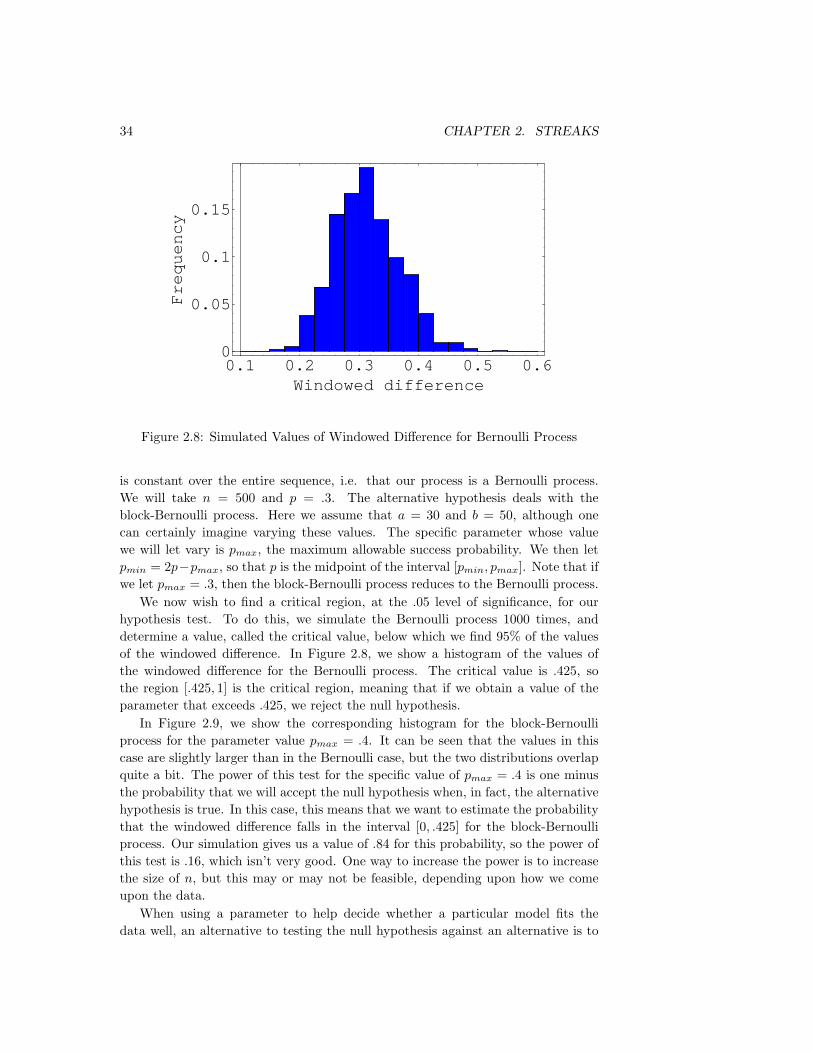
34 CHAPTER 2. STREAKS
0.1 0.2 0.3 0.4 0.5 0.6Windowed difference
0
0.05
0.1
0.15
Frequency
Figure 2.8: Simulated Values of Windowed Difference for Bernoulli Process
is constant over the entire sequence, i.e. that our process is a Bernoulli process.We will take n = 500 and p = .3. The alternative hypothesis deals with theblock-Bernoulli process. Here we assume that a = 30 and b = 50, although onecan certainly imagine varying these values. The specific parameter whose valuewe will let vary is pmax, the maximum allowable success probability. We then letpmin = 2p−pmax, so that p is the midpoint of the interval [pmin, pmax]. Note that ifwe let pmax = .3, then the block-Bernoulli process reduces to the Bernoulli process.
We now wish to find a critical region, at the .05 level of significance, for ourhypothesis test. To do this, we simulate the Bernoulli process 1000 times, anddetermine a value, called the critical value, below which we find 95% of the valuesof the windowed difference. In Figure 2.8, we show a histogram of the values ofthe windowed difference for the Bernoulli process. The critical value is .425, sothe region [.425, 1] is the critical region, meaning that if we obtain a value of theparameter that exceeds .425, we reject the null hypothesis.
In Figure 2.9, we show the corresponding histogram for the block-Bernoulliprocess for the parameter value pmax = .4. It can be seen that the values in thiscase are slightly larger than in the Bernoulli case, but the two distributions overlapquite a bit. The power of this test for the specific value of pmax = .4 is one minusthe probability that we will accept the null hypothesis when, in fact, the alternativehypothesis is true. In this case, this means that we want to estimate the probabilitythat the windowed difference falls in the interval [0, .425] for the block-Bernoulliprocess. Our simulation gives us a value of .84 for this probability, so the power ofthis test is .16, which isn’t very good. One way to increase the power is to increasethe size of n, but this may or may not be feasible, depending upon how we comeupon the data.
When using a parameter to help decide whether a particular model fits thedata well, an alternative to testing the null hypothesis against an alternative is to

2.4. STATISTICAL TESTS ON REPEATED TRIALS 35
0.1 0.2 0.3 0.4 0.5 0.6Windowed difference
0
0.025
0.05
0.075
0.1
0.125
0.15
0.175
Frequency
Figure 2.9: Simulated Values of Windowed Difference for Block-Bernoulli Process
compute and report a p-value of the observed value of the parameter. The p-value ofan observed value is the probability, under the assumption that the null hypothesisis true, that the parameter will take on a value that is at least as extreme as theobserved value.
The phrase “at least as extreme” needs some explanation. Suppose the nullhypothesis is of the form “p = p0” for some parameter p, and the alternativehypothesis is of the form “p > p0.” If a value of p is observed for the parameter p,then the p-value of this observation is the probability, given the null hypothesis istrue, that we would observe a value of p that is at least as large as p (the value thatwas actually observed).
On the other hand, suppose that the alternative hypothesis is of the form “p 6=p0.” In this case the p-value of the observed value p is the probability, given thenull hypothesis is true, that
|p− p0| ≥ |p− p0| .
For a given hypothesis, the smaller the p-value, the less faith we have in themodel as an explanation of the observed data. On the other hand, if we have manydata sets that are supposedly explained by a certain model, then some of the datasets have small p-values, even if the model is correct. To see why this is true,consider the following simple experiment. We have a coin, and we are testing thehypothesis that it is a fair coin, i.e. that the probability of a head coming up whenwe flip the coin is .5. Suppose the coin is fair. Suppose we perform 100 tests ineach of which the coin is flipped 500 times. Then about 5% of the tests will reporta p-value of less than .05. The reason for this is that the observed value p has acertain known distribution, because the null hypothesis is true, and we are usingthis distribution to calculate the p-values of the observations. Since the observationsare distributed according to this known distribution, about 5% of them will have
36 CHAPTER 2. STREAKS
p-values less than .05 (just as about 45% of them, say, will have p-values less than.45).
Another way of looking at this situation is as follows: If we have a large numberof observations under a single model, and the p-values of these observations arefairly uniformly distributed across the interval [0, 1], then the model is doing a goodjob of fitting the data. Of course this does not mean that the model is the only onethat fits the data well, or that it the ‘correct’ one. One should consider other factors,such as the simplicity (or lack thereof) of the various models under consideration,before deciding which model one likes best.
2.4.1 Selection Bias
If one calculates the value of a parameter for a given observation, and the value isseen to be closer to the expected value of that parameter under one model thanunder a second model, one is tempted to state that the first model does a better jobof explaining the observation than does the second model. However, if one selectsonly those observations for which the parameter is closer to the expected value inthe first model than in the second model, then one is guilty of selection bias.
It is also, in general, the case that if one considers more parameters in creating amodel, the model may fit the observed data better than the original, simpler model.For example, since the Markov model subsumes the Bernoulli model, if one includesp1 and p2 as parameters, thereby considering the Markov model, this model willdo a better job of fitting a sequence of 0’s and 1’s than will the Bernoulli model.The trade-off is that the Markov model is more complicated than the Bernoullimodel. If the Bernoulli model does a good job of describing the observations, thanits simplicity should be an argument against its rejection.
Exercises
1 Suppose that we have a sequence of successes and failures of length n. Definep to be the observed proportion of successes, and define p1 to be the observedproportion of successes (excluding the last entry in the sequence, if it is asuccess) that are followed by another success. Define d to be the observednumber of consecutive pairs of entries that are both successes (i.e. the numberof doubletons). Show that if the last entry in the sequence is a failure, then
d = npp1 ,
while if the last entry is a success, then
d = (np− 1)p1 .
Thus, in either case, d is within one of npp1.
2 Can you describe a win-loss sequence for a baseball team that you would sayexhibits streakiness, yet for which the parameter Black is very small?
2.5. DATA FROM VARIOUS SPORTS 37
2.5 Data from Various Sports
2.5.1 Baseball
In baseball, the sequence of hits and outs recorded by a batter in consecutive at-batsis a candidate for study. A plate appearance that results in a walk (or the batterbeing hit by a pitch, or a sacrifice bunt) is not counted as an at-bat, because inthose cases, it is thought that the batter has not been given a chance to hit a well-pitched ball. We remind the reader that even if one uses a Bernoulli trials approachto model such sequences, one should admit that this is only a first approximationto what is actually occurring on the field; presumably the batter’s chance of successin a given at-bat is affected by who is pitching, whether the game is being playedduring the day or at night, how many runners are on base, and many other factors.However, it is still of interest to test the Bernoulli trials model to see how well itfits the data.
We will now apply the various tests described above to our data set. This dataset consists of all players who played in the major leagues between 1978 and 1992,and is taken from the www.retrosheet.org website. We greatly appreciate their laborin creating the files of raw data that we used.
The first test we will apply is the chi-squared test of Albright, described above.For each player and for each season in which that player had at least 150 at-bats, wecomputed the chi-squared value of his sequence of hits and outs, and then computedthe p-value of this chi-squared value. If there is no overall departure from theBernoulli trials model, we would expect to see the p-values uniformly distributedacross the interval [0, 1]. The point here is that even though one might find someseasons for some players for which the p-value is less than some prescribed level ofsignificance, say .05, we should not reject the hypothesis that the Bernoulli trialsmodel fits the data well unless we observe many more than 5% of the p-values below.05.
There were 4786 player-seasons in our data set with the at-bat cutoff of 150.Figure 2.10 shows a histogram of the p-values associated with the chi-squared val-ues for these player-seasons. Since the interval [0, 1] has been partitioned into 20subintervals, uniformity would imply that about 5% of the values occur in eachsub-interval. It can be seen that the p-values are essentially uniform across the unitinterval. In particular, there is no apparent excess of small p-values that wouldcorrespond to large values of the chi-squared parameter (and therefore to eitherstreaky or anti-streaky behavior).
Another pair of parameters to look at is the pair (p1, p2); these are the observedprobabilities of a hit after a hit and after an out, respectively. Under the assumptionof Bernoulli trials, it can be shown that p1−p2 is approximately normally distributedwith a mean and a variance that depend on n and p (we have shown this in theAppendix). In fact, the mean is 0 and the variance is
n + 3np− 1− 5p
qn2.
We can test to see if the hits-outs sequences of baseball players fit the Bernoulli
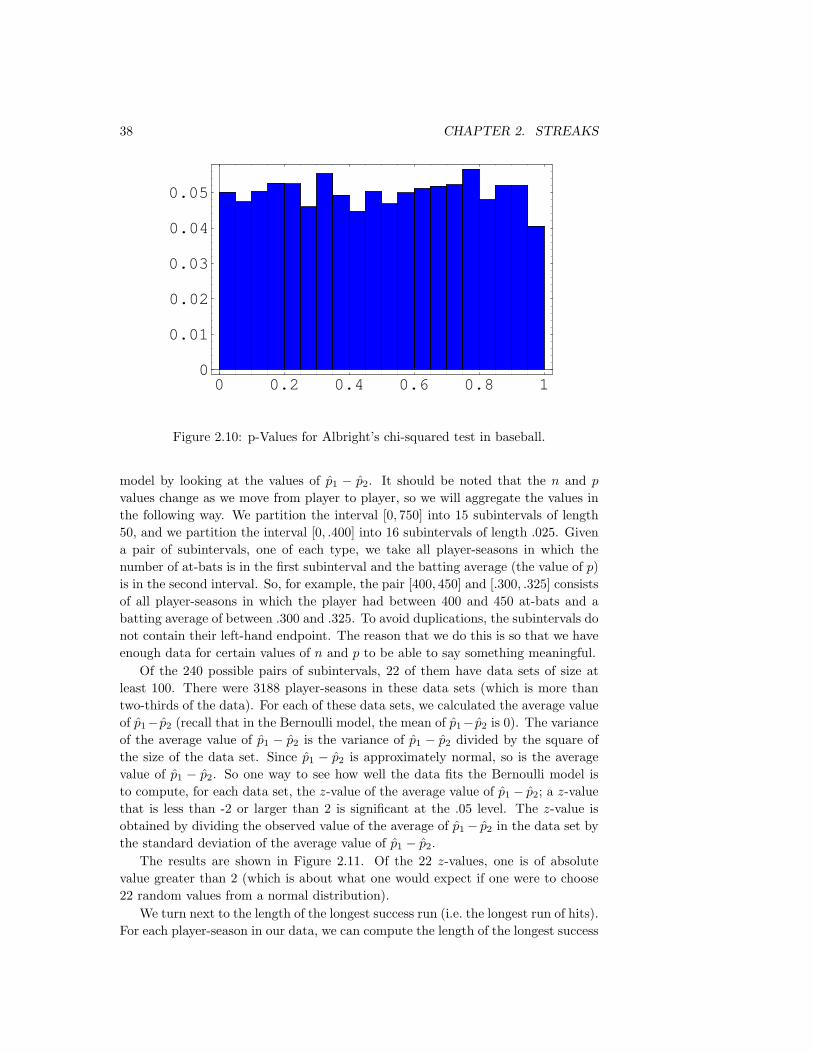
38 CHAPTER 2. STREAKS
0 0.2 0.4 0.6 0.8 10
0.01
0.02
0.03
0.04
0.05
Figure 2.10: p-Values for Albright’s chi-squared test in baseball.
model by looking at the values of p1 − p2. It should be noted that the n and p
values change as we move from player to player, so we will aggregate the values inthe following way. We partition the interval [0, 750] into 15 subintervals of length50, and we partition the interval [0, .400] into 16 subintervals of length .025. Givena pair of subintervals, one of each type, we take all player-seasons in which thenumber of at-bats is in the first subinterval and the batting average (the value of p)is in the second interval. So, for example, the pair [400, 450] and [.300, .325] consistsof all player-seasons in which the player had between 400 and 450 at-bats and abatting average of between .300 and .325. To avoid duplications, the subintervals donot contain their left-hand endpoint. The reason that we do this is so that we haveenough data for certain values of n and p to be able to say something meaningful.
Of the 240 possible pairs of subintervals, 22 of them have data sets of size atleast 100. There were 3188 player-seasons in these data sets (which is more thantwo-thirds of the data). For each of these data sets, we calculated the average valueof p1− p2 (recall that in the Bernoulli model, the mean of p1− p2 is 0). The varianceof the average value of p1 − p2 is the variance of p1 − p2 divided by the square ofthe size of the data set. Since p1 − p2 is approximately normal, so is the averagevalue of p1 − p2. So one way to see how well the data fits the Bernoulli model isto compute, for each data set, the z-value of the average value of p1 − p2; a z-valuethat is less than -2 or larger than 2 is significant at the .05 level. The z-value isobtained by dividing the observed value of the average of p1− p2 in the data set bythe standard deviation of the average value of p1 − p2.
The results are shown in Figure 2.11. Of the 22 z-values, one is of absolutevalue greater than 2 (which is about what one would expect if one were to choose22 random values from a normal distribution).
We turn next to the length of the longest success run (i.e. the longest run of hits).For each player-season in our data, we can compute the length of the longest success

2.5. DATA FROM VARIOUS SPORTS 39
0 5 10 15 20Group number
-2
-1
0
1
2
3
z-value
Figure 2.11: z-Values for the Average of p1 − p2.
run. However, in the Bernoulli model, the distribution of this length depends uponboth n, the length of the sequence (in this case, the number of at-bats), and p,the probability of a success in an individual trial (in this case, the batting average).The Markov model depends upon n, p, and p1, the probability of a success followinga success. We would like to be able to display the aggregate data against thepredictions made by both models.
In the case of the Bernoulli model, we can proceed in several ways. Our firstmethod of comparison will be carried out as follows. For each of the 4786 player-seasons with at least 150 at-bats, we will simulate a season using Bernoulli trialswith the same number of at-bats and batting average as the actual season. Then wewill observe the longest run of successes in each of these simulated seasons. Finally,we will compare the distribution of the lengths of the longest run of successes inthe simulated seasons with the corresponding distribution in the actual data.
When we carry this procedure out, we obtain the results shown in Figure 2.12.The horizontal coordinate represents the length of the longest success run in eachplayer-season, and the vertical coordinate represents the observed frequencies. Thefit between the simulated and actual data is quite good. In addition, the readerwill recall Figure 2.3, which shows that in the Markov model, if p1 > p, then thedistribution of the longest success run is shifted to the right from the correspondingdistribution in the Bernoulli model. The aggregate data does not show any suchshift.
Another way to compare the Bernoulli model with the data is to proceed aswe did above with the distribution of p1 − p2. We will group the data using pairsof subintervals, so that the numbers of at-bats and the batting averages are closeto equal across the group. Then, for each group, we will compute the distributionof the longest success run and compare it with the theoretical distribution. Thiscomparison will be carried out using a chi-square test. For each of the 22 groups we

40 CHAPTER 2. STREAKS
2 4 6 8 10Length of longest success run
0
0.1
0.2
0.3
Probability
Figure 2.12: Distributions of Simulated and Actual Longest Success Runs.
used above (those containing at least 100 player-seasons) we will report a p-valuefor the chi-square value.
In Figure 2.13, we show the results of the above calculations. For each of the 22groups of data containing at least 100 player-seasons, the observed and theoreticalaverage length of the longest success run; the theoretical average is obtained byusing, for each group, the average number of at-bats and the average success prob-ability. As can be seen, the fit is very good; the relative error is never greater than6%, and only twice is it as large as 4%. For each of the 22 data sets, we also com-pute the chi-squared value of the comparison between the theoretical and observeddistributions, and then compute the p-values corresponding to these chi-squaredvalues. Figure 2.14 shows the 22 p-values. These p-values show that the Bernoullimodel does a very good job of fitting the data.
It has been suggested that there might be a qualitative difference between successruns and failure runs. The thought was that while success runs are limited in lengthby the skill of the batter, failure runs might, in some cases, continue longer thanpredicted because the hitter will spiral downwards psychologically during a slump.We ran the above tests again on the same 22 groups, this time looking at thelongest failure runs. The p-values, corresponding to those in Figure 2.14, are shownin Figure 2.15. It can be seen that once again, the fit is very good.
Another aspect of baseball that has been taken to provide evidence in favor ofstreakiness is the idea of a hitting streak. A hitting streak by a player is a set ofconsecutive games played by the player in which he gets at least one hit in eachgame. In order to qualify as a hitting streak, the games must all occur in a singleseason. The longest hitting streak that has ever occurred in the major leagueslasted 56 games; it happened in 1941, and the player who accomplished this streakwas Joe DiMaggio. Much has been written about this streak (see, for example, [3],[6], and [10]). The question that we wish to consider is whether the fact that this

2.5. DATA FROM VARIOUS SPORTS 41
5 10 15 20Group number
0
1
2
3
4
Avg.
length
Figure 2.13: Observed vs. Theoretical Longest Success Run Lengths.
0 5 10 15 20Group number
0
0.2
0.4
0.6
0.8
p-value
Figure 2.14: p-Values for Chi-Squared Comparison of Longest Success Run Data.

42 CHAPTER 2. STREAKS
0 5 10 15 20Group number
0
0.2
0.4
0.6
0.8p-value
Figure 2.15: p-Values for Chi-Squared Comparison of Longest Failure Run Data.
streak occurred provides evidence against the Bernoulli trials model.If a hitter has a fixed number of at-bats in each game, then it is fairly easy to
calculate the probability that he will hit safely in n consecutive games, assumingthe Bernoulli model. For example, if a hitter has a .350 batting average, and hasfour at-bats in each game, then, under the Bernoulli model, the probability that hegets at least one hit in a given game is
1− (.650)4 = .8215 .
Thus, in a given set of 56 consecutive games, the probability that the hitter gets atleast one hit in each game is
(.8215)56 = .0000165 .
This sounds like a very unlikely event, but we’re not really asking the right question.A slightly better question might be the following: Given that a hitter plays in 154games in a season, and has a season batting average of .350, what is the probabilitythat he bats safely for at least 56 games? (We use 154 for the length of a season,since almost all of the player seasons with batting averages of at least .350 occurredbefore the seasons were lengthened to 162 games.) Once again, under the Bernoullimodel, we can answer this question rather easily. Putting this question in terms ofideas that we have already introduced, this question is equivalent to asking whatis the probability, in a Bernoulli trials sequence of length 154, and with successprobability .8215, that the longest success run is at least of length 56. The question,in a form similar to this one, was considered in [14]. The answer, in this case, is.0003.
Of course, there have been many batters who have had season batting averagesof much higher than .350, and it is clear that as the batting average climbs, so does

2.5. DATA FROM VARIOUS SPORTS 43
0.3 0.32 0.34 0.36 0.38 0.4 0.42Batting average
0
0.0025
0.005
0.0075
0.01
0.0125
0.015
0.0175
Probability
Figure 2.16: Probability of a hitting streak of at least 56 games.
the probability of having a long hitting streak. Figure 2.16 shows the probability ofa hitting streak of at least 56 games in a 154-game season as a function of the seasonbatting average. This figure shows that the season batting average has a large effecton the probability of a long hitting streak. Figure 2.17 shows a histogram of playerseasons since 1901 for which the batting average was at least .340.
We still are not asking quite the right question. There are two changes that weshould make. First, we do not want to know the probability that a given hitter willhave a long hitting streak; rather, we want to know the probability that at leastone of a set of hitters will have a long hitting streak. We will take this set of hittersto correspond to all hitters since 1901 who batted at least .340 in a season and hadat least 300 at-bats (there were 430 such seasons). We are arbitrarily disregardinghitters whose batting averages are below .340.
The second change that should be made concerns the variability of the number ofat-bats belonging to an individual player over a set of games. It should be clear thatif a batter averages four at-bats per game, but the number of at-bats varies widelyover a set of games, then it is less likely that he will have a long hitting streak. Asa simple example to help show this, consider a batter with a .350 batting averageunder the following two scenarios: first, he gets exactly four at-bats in each of 10consecutive games, and second, he gets, alternatively, two and six at-bats in 10consecutive games. In the first case, the probability that he gets at least one hit ineach game is (
1− (.650)4)10
= .13997 .
In the second case, the probability is(1− (.650)2
)5(1− (.650)6)5
)= .04400 .
So, here is the question that we want to try to answer: Suppose we restrict our

44 CHAPTER 2. STREAKS
0.34 0.36 0.38 0.4 0.42Batting average
0
5
10
15
20
25Number
of
seasons
Figure 2.17: Number of player seasons with a given batting average.
attention to those player-seasons in which the player batted at least .340 (we willcall this set our good-hitter data set), and suppose we take into account the typicalvariation between games of the number of at-bats of a player in a game. What isthe probability, under the Bernoulli trials model, that at least one of the playerswould have a hitting streak of at least 56 games?
This is too complicated a question to hope for a theoretical answer, but wecan simulate the seasons of these hitters, using the observed batting averages andnumbers of games and at-bats. Here is how the simulation is carried out. We beginby finding an estimate for the standard deviation in the sequence of numbers ofat-bats in a game, over a typical player season. We can use our original data setfrom the years 1978 to 1992 to obtain this estimate. We restrict our attention tothose players who batted at least .300 for the season, and who had at least 300at-bats. There were 369 player seasons that satisfied these requirements. For eachsuch season, we found the sequence of numbers of at-bats in all games started bythe player. The reason for this restriction is that the players in our good-hitter dataset started almost every game in which they played. For each of these 369 seasons,we compute the standard deviation of the sequence of at-bats. Then we computethe average of these standard deviations. When we do this, we obtain a value of.8523.
For each player-season in our good-hitter data set, we will produce a sequenceof at-bats per game for the number of games in which the player participated thatseason. The terms of this sequence will be drawn from a normal distribution withmean equal to the average number of at-bats by the player during that season, andwith standard deviation equal to .8523. The terms will be rounded to the nearestinteger, so that they represent numbers of at-bats (which must be integers). If aninteger in the sequence is less than or equal to 0, we throw it out. The reason forthis is that a hitting streak is not considered to be interrupted if a player appears

2.5. DATA FROM VARIOUS SPORTS 45
0 200 400 600 800 1000Simulation number
40
50
60
70
80
90
Longest
streak
Figure 2.18: Simulated longest hitting streak data.
in a game but does not record any official at-bats.Since we are operating under the assumption of Bernoulli trials, we use the
player’s season batting average to simulate his season with the above simulatedat-bat sequence. We then record the longest hitting streak in the season. We dothis for each player, and record the longest hitting streak among all of the players.To estimate the probability that someone would have a hitting streak of at least 56games, we carry out the above procedure many times, and calculate the fraction ofthose trials that lead to at least one such streak.
The results of the simulation are shown in Figure 2.18. The above procedurewas carried out 1000 times. In the simulated data, the length of the longest hittingstreak ranged from 33 to 85, and 126 times the length was at least 56 games.This simulation shows that the probability, under the Bernoulli trials model, thatwe would observe a hitting streak of at least 56 games in length is about 1/8(≈ 126/1000) and thus Joe DiMaggio’s streak does not cast doubts on the meritsof this model. The simulation also shows that viewed from this angle, DiMaggio’sfeat is probably not the most amazing feat in all of sports, or even in baseball.
One can consider another question that is usually raised when DiMaggio’s streakis discussed; that is the question of whether anyone will ever break his record.Predicting the future is a dangerous business, but one can use the above simulations,together with known data, to say something of interest. Of the 430 player seasonsin which the player batted at least .340, about three-quarters of them occurredin the period 1901-1950. Thus, the rate at which .340 seasons occur has changeddramatically over the years. Figure 2.19 shows the moving average of the numberof .340-plus player seasons, averaged over ten-year windows. Currently, the averagenumber of such player seasons is about 4 per year. Thus we assume that there willbe about 4 such player seasons in each year in the future. We have seen that in 430such player seasons, the probability is about 1/8 that someone will have a 56-game

46 CHAPTER 2. STREAKS
1920 1940 1960 1980 2000Year
0
2
4
6
8
10
12
14Rate
of
.340+
seasons
Figure 2.19: Moving average number of .340+ player seasons.
hitting streak. Thus, we should expect to see one in the next 3440 (= 8× 430) suchplayer seasons, which translates to 860 years. Putting it another way, it seems veryunlikely that we will see such a streak in any of our lifetimes. Viewed from thisperspective, DiMaggio’s streak seems much more impressive than before.
There is another way to estimate how long it might be until the record is broken.It was stated above that the probability is .0003 that a .350 hitter will have a hittingstreak of at least 56 games in a season. If there are about 4 such seasons per yearin the future, we would expect to see such a streak, assuming the Bernoulli trialsmodel, every 1/(.0003× 4) = 833 years.
The above argument does not take into account the incredible pressure thatwill surely be felt by any player who approaches the record. Joe DiMaggio musthave felt pressure as well during the streak, but once he had broken the existingrecord of 44 consecutive games, the pressure probably abated quite a bit. Thus,any player who threatens DiMaggio’s record will feel pressure for quite a bit longerthan DiMaggio did. Of course, those who believe that Bernolli trials are a goodmodel for hitting in baseball might argue that the pressure under which a playerfinds himself in such a situation is irrelevant.
We now turn to team statistics; we seek to answer the question of whether teamsexhibit streaky behavior. One way to check this is to recall that if a process has apositive autocorrelation (meaning that the probability of a success in a given trialincreases if the previous trial is a success), then the lengths of the longest streakswill, on average, be longer than in the Bernoulli trials model. This will be true ofboth winning and losing streaks.
There are 390 team seasons in our data set. For each of these seasons, wecomputed the lengths of the longest winning and losing streaks. Then we groupedthe team seasons by rounding the winning percentages to the nearest multiple of.01 (so, for example, a winning percentage of .564 is rounded to .56). For each

2.5. DATA FROM VARIOUS SPORTS 47
0.35 0.4 0.45 0.5 0.55 0.6 0.65Winning percentage
4
6
8
10
Avg.
length
Figure 2.20: Actual and Theoretical Longest Winning Streak Lengths.
group, we calculated the average lengths of the longest winning and losing streaks.Figures 2.20 and 2.21 show these average lengths, as well as the average lengthsin the Bernoulli trials model. We note that the fit between the actual and thetheoretical longest streak lengths is very good, except perhaps at the ends of thegraphs. But even at the ends, there is no bias; the reason for the large deviationsis that the group sizes are so small. Of the 390 team seasons in the data set, only9 have rounded winning percentages that lie outside of the interval [.36, .64].
In the book Curve Ball[1], the authors, Jim Albert and Jay Bennett, study thequestion of team streakinenss, in the sense of the block-Bernoulli process. Specif-ically, their model of streaky behavior is as follows: A hypothetical season is splitinto nine non-overlapping blocks of 18 games each (so in our notation, a = b = 18).Three winning percentages are computed, denoted by pC, pav, and pH (for cold, av-erage, and hot). The percentage pav is the team’s season winning percentage. Thepercentages pC and pH are defined to be .1 less than and more than pav, respec-tively. So this is somewhat like our pmin and pmax, except that in their model, theblock winning percentages are not uniformly chosen in the interval [pC, pH]; rather,there are only three possible block winning percentages. Finally, each of these threeblock winning percentages is assigned randomly to three of the nine 18-game blocks.Figure 2.22 shows an example of the block winning percentages for a team whoseseason percentage is .55.
A team whose win-loss sequence arises from the above block-Bernoulli processwill be said to be streaky, while one whose win-loss sequence arises from a Bernoulliprocess will be called consistent. Of course, we do not expect all teams to behavein one of these two ways; we need a parameter that can be calculated, and thatdoes a good job of distinguishing between these two models. As we said above,our windowed difference parameter does not distinguish very well between the twomodels we posited.

48 CHAPTER 2. STREAKS
0.35 0.4 0.45 0.5 0.55 0.6 0.65Winning percentage
4
6
8
10
12
14
Avg.
length
Figure 2.21: Actual and Theoretical Longest Losing Streak Lengths.
0 25 50 75 100 125 150Game number
0.45
0.5
0.55
0.6
0.65
Winning
percentage
Figure 2.22: Block winning percentages for a streaky team

2.5. DATA FROM VARIOUS SPORTS 49
0 20 40 60 80 100 120 140Game number
0.2
0.4
0.6
0.8
1
Winning
percentage
Figure 2.23: Windowed winning percentage for 1984 Baltimore Orioles
Albert and Bennett define their parameter, called Black, as follows. Given ateam’s win-loss sequence for a season, they compute the windowed winning per-centages for all blocks of 12 games (so in a 162-game season, there are 151 suchblocks, starting at games 1 to 151). They plot these percentages, along with a hori-zontal line whose y-value is the season winning percentage. An example of this plotis shown in Figure 2.23; the team is the 1984 Baltimore Orioles. The parameterBlack is easy to describe in terms of this figure; it is the area of the black region.
It is clear that if a team is consistent, then Black will be very small, while if ateam is streaky, Black will probably be large. Thus, this parameter might be ableto distinguish between the block-Bernoulli and the Bernoulli models. To decidewhich model fits a given team better, Albert and Bennett compute the winningpercentage, call it p, of the team. Then they obtain, by simulation, the distributionof the parameter Black under both models. The actual value of Black for the teamis computed, and compared with the two distributions. For each distribution, ap-value is reported. If the first p-value of the observation is larger than the secondp-value, then they claim that the first model fits the team’s performance betterthan the second model.
In fact, they go further and use the ratio of the p-values as the odds that theteam is consistent (or streaky). For example, if the p-values for a given team, underthe consistent and streaky models, are .08 and .30, respectively, then they say thatthe probability that the team is streaky is .79 (= .30/(.08 + .30)). This is a fairlyloose use of the word ‘probability,’ since there is no obvious experiment or samplespace on which this probability is based.
We will proceed in a different direction with the parameter Black. We are tryingto determine whether the Bernoulli model does a good job of fitting the win-losssequences in our data set. For each of the 390 teams in this data set, we cancalculate a p-value for the observed value of Black, under the null hypothesis of

50 CHAPTER 2. STREAKS
0 100 200 300Team number
0
0.2
0.4
0.6
0.8
1p-value
Figure 2.24: p-values for the Black parameter
the Bernoulli model. For each team, we use the winning percentage of that team,rounded to the nearest .01, to compute a simulated distribution for Black. If thereare more streaky teams than can be explained well by the Bernoulli model, weshould see more small p-values than expected, i.e. the set of p-values should notbe uniformly distributed across the interval [0, 1]. (The reason that the p-valuesof streaky teams are small is because the parameter Black is very large for suchteams, and large values of Black correspond to small p-values.) Figure 2.24 showsthis set of p-values. The set has been sorted. If the set were perfectly uniformlydistributed across [0, 1], the graph would be the straight line shown in the figure.One sees that the set of p-values is very close to uniform, and in addition, thereare certainly no more small p-values than expected under the Bernoulli model. Infact, we see that there are slightly more teams with large p-values than might beexpected. Since large p-values correspond to small values of Black, this says thatthe number of very consistent teams is slightly more than expected.
2.5.2 Basketball
The most widely referenced article on streaks in sports is undoubtedly the paperby Gilovich, Vallone, and Tversky[5]. This article examines whether or not thereis auto-correlation in the shooting sequences of basketball players. The authorssurveyed fans, collected data from games at both the professional and college level,and carried out a set of experiments with amateur subjects. We will give some oftheir most intriguing findings here.
In a survey of more than 100 basketball fans, recruited from the student bodiesof Cornell and Stanford, 91% believed that a player was more likely to make hisnext shot if he had made the last two or three shots than if he had missed the lasttwo or three shots. In addition, 68% said the same thing when asked about free
2.5. DATA FROM VARIOUS SPORTS 51
throws. The fans were then asked to consider a hypothetical basketball player whohas a field goal percentage of 50% (i.e. he makes about one-half of his shots). Theywere asked to estimate the player’s field goal percentage for those shots that occurafter he has made a shot, and for those shots that occur after he has missed a shot(these numbers are our p1 and p2). The average value of their estimate for p1 was.61, and for p2 it was .42. In addition, the former estimate was greater than thelatter estimate for all of the fans in the survey.
The authors compared these estimates with data obtained from 48 games in-volving the Philadelphia 76ers in the 1980-81 season. The data consisted of thesequences of hits and misses for all of the field goal attempts for all of the playerson the 76ers. Among the more interesting observations is the fact that for eightof the nine major players on the team, the probability that they made a shot washigher after a miss than after a hit. For these players, the weighted mean of theirfield goal percentages (the average of their probabilities of making a field goal,weighted by the number of attempts) was .52. The weighted mean of their fieldgoal percentages after a miss and a hit were .54 and .51, respectively.
In their paper, the authors performed other statistical tests, including a runstest, a test of stationarity, and a test for stability of shooting percentage acrossgames. None of these test provided any strong evidence for rejecting the Bernoullimodel.
They also looked at free throw data from the Boston Celtic teams in the 1980-81and 1981-82 seasons, and again found no evidence of streakiness. Finally, they re-cruited members of the Cornell basketball teams (both men and women) to take partin a controlled shooting experiment. Each participant was asked to take 100 shotsfrom a distance at which their accuracy was roughly 50%. They were paid money,where the amount was based both on how accurately they shot and how accuratelythey predicted their next shot. Once again, there was no evidence suggesting theexistence of streakiness.
We now turn to another aspect of basketball in which there is some evidencethat fans think there is streakiness. In much of the world, money is bet on almostall aspects of sports. In the United States, for example, one can bet on professionalbasketball in several ways. One of the most popular ways proceeds as follows.Professional odds-makers (called bookies) set a point spread before the beginningof a game. For example, if the Lakers are playing the Spurs, the bookies may saythat the Spurs are favored by 5.5 points. A bettor can bet on either team; if hebets on the Lakers, he is given 5.5 points, meaning that if the Lakers win the game,or if they lose by 5 points or fewer, then the bettor wins. Conversely, if he bets onthe Spurs, then the bettor wins only if the Spurs win by at least 6 points.
The bookies’ take 10% (called a vigorish, or vig) of the winning bets and all ofthe losing bets. In many cases, the bookies do not set the point spread at theirprediction for the game. The bookies’ objective is to have an equal amount ofmoney bet on both teams. To see why they want this, suppose first that $10,000 isbet on each team. Then the bookies make $1,000, regardless of which team beatsthe spread. However, if $15,000 is bet on the Lakers, and $5,000 is bet on the Spurs,and the Lakers beat the spread, then the bookies must pay out $13,500 and only
52 CHAPTER 2. STREAKS
take in $5,000, so they lose $8,500.In a paper that appeared in 1989[4], Colin Camerer showed that the bettors,
and hence the bookies, believed in streaky behavior in the NBA (the professionalbasketball league in the United States). Camerer collected data on all games playedin three seasons of the NBA (from 1983 to 1986). His data set consists of the scoresof all of the games, and the point spreads set by a popular bookie in Las Vegas.
At the beginning of every game (except for the first game played by a team ina season), each team has a winning streak or a losing streak. Each game is putinto a subset depending upon the lengths of these two streaks. For example, if thefirst team has a three-game winning streak and the second team has a two-gamelosing streak, then the game is put into the (+3,−2) subset. The longer of the twostreaks determines which of the two teams is the ‘first’ team; if the streaks are ofequal length, then a coin flip determines which team is the first team. Thus, eachgame appears in exactly one subset. For each subset, the fraction of those gamesin which the first team beat the spread was calculated.
This fraction is very important for the following reason. Camerer’s data show,for example, that the subsets of the form (+4, k), with 1 ≤ k ≤ 4, have a combinedfraction of .46, this means that 46% of the teams with four-game winning streakswho played teams with shorter streaks managed to beat the spread. This can betaken as evidence that the bettors (and hence the bookies) overvalued the teamswith four-game winning streaks. The question of whether such a fraction is signif-icant can be answered using standard statistical methods. We will now show howthis is done using the above data.
In order to proceed, we need one more parameter about our data subset, namelyits size. There were 159 games in the subsets that we are dealing with. Supposethat we assume the probability that the first team will beat the spread is .5. Whatis the probability that in 159 trials, the first team will actually beat the spread 46%of the time or less, or equivalently, in at most 73 games? The answer is about .17,which a statistician would not regard as significant.
The data can be pooled by considering all of the subsets (j, k) with j positive(and j ≥ |k|). There were 1208 games of this type, and the first team beat thespread 47.9% of the time. We can once again ask the question, if a fair coin isflipped 1208 times, what is the probability that we would see no more than 579(= .479 × 1208) heads? We can calculate this exactly, using a computer, or wecan find an accurate approximation, by recalling that the number of heads NH is abinomially distributed random variable with mean equal to 604 (= 1208 × .5) andstandard deviation equal to 17.38 (=
√1208× .5× .5). Thus, the expression
NH − 60417.38
has, approximately, a standard normal distribution. The value of this expressionin the present case is -1.44. The probability that a standard normal distributiontakes on a value of -1.44 or less is about .0749, which is thus the p-value of theobservation. This observation is therefore significant at the 10% level, but not atthe 5% level.

2.5. DATA FROM VARIOUS SPORTS 53
If one instead takes all of the subsets of the form (j, k) with j ≥ 3 and j ≥ |k|,there are 698 games, and the first team beat the spread in 318 of these games. Thisrepresents 45.6% of the games. What is the p-value of this observation? It turnsout to be about .0095, which is a very small p-value.
One can also look at the corresponding pooled data for teams with losing streaks.There were 1140 games in the subsets of the form (j, k), with j ≤ −1 and |j| ≥ |k|,and the first team beat the spread in 597 of these games. The p-value of thisobservation is .055. If we restrict our attention to those subsets for which j ≤ −3and |j| ≥ |k|, there were 643 games, and the first team beat the spread in 340 ofthese games. The p-value of this observation is .0721.
There are two more collections of subsets that are worth mentioning. The firstis the collection of subsets of the form (j, k), with j negative and k positive (and|j| ≥ |k|). If one does not believe in streaks, then one would think that in thiscase, bettors would undervalue the first team’s chances of beating the spread, sincethe first team is on a losing streak and the second team is on a winning streak.Thus, the first team should beat the spread more than half the time. There were670 games in this collection of subsets, and the first team beat the spread in 356 ofthese games, or 53.1% of the time, leading to a p-value of .0526. Interestingly, inthe corresponding collection, in which the first team is on a winning streak and thesecond team is on a losing streak of equal or smaller length, the first team beat thespread in 358 games, which is 50.1% of the time. The p-value of this observationis, of course, .5.
Although only one of the six p-values reported above is less than .05, five of themare rather small, and thus there is some evidence that the bettors are overvaluingteams with winning streaks and under-valuing those with losing streaks.
If the astute bettor realizes that the average bettor is overvaluing teams withlong winning streaks and undervaluing teams with long losing streaks, can he or shemake money on this information? In Exercise 1, the reader is asked to show that ifthere is a 10% vig, then the bettor needs to win 52.4% of the time (assuming he isbetting constant amounts) to break even. A few of the pooled subsets mentionedabove had winning percentages that were at least 2.4% away from 50% in onedirection or the other, meaning that had one made bets, in the correct direction, onall of the games in that pooled subset, one could have made money. Unfortunately,if one tests the hypothesis that the winning percentage in any of the pooled subsetsis at least 52.4%, one finds that none of the results are significant at the 5% level.
The results for the 2003-04 season are qualitatively different than those found byCamerer. Through the All-Star break (February 15, 2004), teams having a winningstreak, playing teams with equal or shorter streaks, beat the spread in 193 out of370 games, or 52.2% of the games. Teams having a losing streak, playing teamswith equal or shorter streaks, beat the spread in 179 out of 375 games, or 47.7%of the games. Thus, betting on teams with winning streaks, and betting againstteams with losing streaks, would have resulted in a winning percentage of 52.2%.Note that this is the opposite of what happened in Camerer’s data. Does the readerthink that this change will persist, and if so, is it because the bettors have gottensmarter (i.e. have they incorporated the fact that streaks are over-rated into their
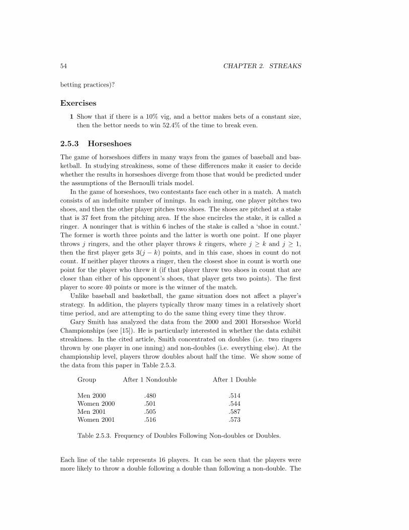
54 CHAPTER 2. STREAKS
betting practices)?
Exercises
1 Show that if there is a 10% vig, and a bettor makes bets of a constant size,then the bettor needs to win 52.4% of the time to break even.
2.5.3 Horseshoes
The game of horseshoes differs in many ways from the games of baseball and bas-ketball. In studying streakiness, some of these differences make it easier to decidewhether the results in horseshoes diverge from those that would be predicted underthe assumptions of the Bernoulli trials model.
In the game of horseshoes, two contestants face each other in a match. A matchconsists of an indefinite number of innings. In each inning, one player pitches twoshoes, and then the other player pitches two shoes. The shoes are pitched at a stakethat is 37 feet from the pitching area. If the shoe encircles the stake, it is called aringer. A nonringer that is within 6 inches of the stake is called a ‘shoe in count.’The former is worth three points and the latter is worth one point. If one playerthrows j ringers, and the other player throws k ringers, where j ≥ k and j ≥ 1,then the first player gets 3(j − k) points, and in this case, shoes in count do notcount. If neither player throws a ringer, then the closest shoe in count is worth onepoint for the player who threw it (if that player threw two shoes in count that arecloser than either of his opponent’s shoes, that player gets two points). The firstplayer to score 40 points or more is the winner of the match.
Unlike baseball and basketball, the game situation does not affect a player’sstrategy. In addition, the players typically throw many times in a relatively shorttime period, and are attempting to do the same thing every time they throw.
Gary Smith has analyzed the data from the 2000 and 2001 Horseshoe WorldChampionships (see [15]). He is particularly interested in whether the data exhibitstreakiness. In the cited article, Smith concentrated on doubles (i.e. two ringersthrown by one player in one inning) and non-doubles (i.e. everything else). At thechampionship level, players throw doubles about half the time. We show some ofthe data from this paper in Table 2.5.3.
Group After 1 Nondouble After 1 Double
Men 2000 .480 .514Women 2000 .501 .544Men 2001 .505 .587Women 2001 .516 .573
Table 2.5.3. Frequency of Doubles Following Non-doubles or Doubles.
Each line of the table represents 16 players. It can be seen that the players weremore likely to throw a double following a double than following a non-double. The

2.5. DATA FROM VARIOUS SPORTS 55
table gives the average frequencies over sets of players. A breakdown of the datashows that of the 64 players, 25 of the men and 26 of the women were more likely tothrow a double following a double than following a non-double (we will refer to thissituation as positive auto-correlation, as before). That this is evidence of streakinesscan be seen as follows. If players were not affected by their throws in the precedinginning, then about half of them would have positive auto-correlation. Continuingunder the assumption of independence between innings, we see that the probabilityof observing as many as 51 of the 64 players with positive auto-correlation is thesame as the probability that if a fair coin is flipped 64 times, it comes up heads atleast 51 times. This probability is approximately .0000009.
At the championship level, the players’ probabilities of throwing a double in anygiven inning is so high that using either the length of the longest run of doubles orthe number of runs of doubles and non-doubles cannot be used to reject the nullhypothesis of Bernoulli trials at the 5% level. For example, one of the players in the2000 championships pitched 13 doubles in 14 innings. This means that there wereeither two or three runs of either type. But under the null hypothesis of Bernoullitrials, using the value p = 13/14, there is a probability of ,143 of two runs (and aprobability of .857 of three runs), so in this case, even if there are two runs, thep-value is much larger than .05.
Smith gets around this problem by calculating, under the null hypothesis, theexpected number of runs by a given player in a given game, and then tabulatingthe number of games in which the actual number of runs was above or below theexpected number. Fewer runs than expected mean streakiness. Table 2.2 shows thenumber of games with fewer or more runs than expected for each championship,together with the p-values for the observations, under the null hypothesis.
Group Fewer Runs More Runs p-value
Men 2000 129 107 0.0857Women 2000 136 103 0.0191Men 2001 137 98 0.0065Women 2001 138 99 0.0067
Table 2.5.3. Number of Games with Fewer or More Runs than Expected.
2.5.4 Tennis
The game of tennis is interesting in probability theory because it provides an exam-ple of a nested set of Markov chains. The reader will recall that, roughly speaking,a Markov chain is a process in which there is a set of states and a transition matrixwhose entries give the probabilities of moving from any state to any other state inone step. The chain can either be started in a specific state, or it can be started witha certain initial distribution among the states. We will describe the various Markovchains that make up a tennis match, and then give some results about tennis thatfollow from elementary Markov chain theory. We will then look at whether or nottennis is streaky at the professional level.

56 CHAPTER 2. STREAKS
A tennis match is divided into sets; in most cases, the first person to win twosets is the winner of the match. (There are a few professional tournaments in whichthe winner is the first person to win three sets.) The set scores in an on-going tennismatch can be thought of as labels in a Markov chain. The possible scores, from thepoint of view of one player are 0-0 (at the beginning of the match), 1-0, 0-1, 1-1,2-0, 2-1, 1-2, and 0-2. The last four of these states are said to be absorbing states,because once the match enters one of these states, it never leaves the state. Theother four states are called transient states, because if the match is in one of thesestates at a given time, it will leave at the next step. (In a general absorbing Markovchain, a state is called transient if it possible for the chain to go from that state toan absorbing state in a finite number of steps. It is not necessary that the chainalways leave the transient state in one step.)
Suppose that player A has probability p of winning a set against player B. Then,for example, the probability that the Markov chain will move from state 0-1 to state1-1 is p, while the probability that it will move from state 1-1 to state 1-2 is 1− p.The reader can check that if the above states are numbered from 1 to 8, and wedenote by pij the probability of moving from state i to state j in one step, then thetransition matrix P = (pij) is given by
P =
0-0 1-0 0-1 1-1 2-0 2-1 1-2 0-2
0-0 0 p 1− p 0 0 0 0 0
1-0 0 0 0 1− p p 0 0 0
0-1 0 0 0 p 0 0 0 1− p
1-1 0 0 0 0 0 p 1− p 0
2-0 0 0 0 0 1 0 0 0
2-1 0 0 0 0 0 1 0 0
1-2 0 0 0 0 0 0 1 0
0-2 0 0 0 0 0 0 0 1
It turns out that we will want to split most of the above states into two statesin our final model, because it is thought that the serve in tennis has a large effecton who wins a given game; thus, it will be important for us to record who is servingat the beginning of each set. We will discuss this in more detail below.
Each set in tennis consists of a number of games. The first player to win sixgames, if his or her opponent has won at most four games, wins the set. If the scoreis 6-5, the set continues until it is either 7-5, in which case the player with sevengames wins, or it is 6-6, in which case a tie-breaker is played. Whoever wins thetiebreaker wins the set. Thus a set can be modeled by an absorbing Markov chain.

2.5. DATA FROM VARIOUS SPORTS 57
0 0.2 0.4 0.6 0.8 1Point-winning probability
0
0.2
0.4
0.6
0.8
1
Game-winning
prob.
Figure 2.25: Game-winning vs. point-winning probabilities in tennis.
Both a regular game and a tie-breaker are themselves absorbing Markov chains.In a game, the first person to win at least four points and be at least two pointsahead wins the game. In a tie-breaker, the first person to win at least seven pointsand be at least two points ahead wins the tie-breaker.
At the professional level, the person who is serving a point has a much greaterthan even chance of winning the point. In the authors’ opinion, this advantage maynot extend down to their level. Since our data comes from professional matches, weneed to take account of the serve. In each non-tie-break game, one person serves allof the points. The service rotation in a tie-break is more complicated; one playerstarts the tie-break by serving one point, and then the players take turns servingtwo consecutive points.
We show, in Figure 2.25, the probability that a player wins a game that he isserving, if he has a probability p of winning any given point. This graph shows thatif p = .6, then the player will win the game with probability .74, and if p = .8, thenthe player will win the game with probability .98.
Now suppose that two players are playing a best-of-three set match in which thefirst player has a probability of p of winning any given point (so in this case, we areassuming that the serve does not affect the outcome of the point). In Figure 2.26,we show the probability of the first player winning the match, as a function of p.Note that even if p = .51, the probability that the first player wins the match is.748.
How are such probabilities determined? We will briefly describe the calculationsthat are needed, and the theorems on which these calculations are based. For moreexamples, and for proofs of the theorems, the reader is referred to [7].
If P is the transition matrix of an absorbing Markov chain, then we can relabelthe states so that the first set of states are the transient ones, and the last set ofstates are the absorbing ones. If we do so, the matrix P assumes the following

58 CHAPTER 2. STREAKS
0.5 0.6 0.7 0.8 0.9Point probability
0.6
0.7
0.8
0.9
1Match
probability
Figure 2.26: Match-winning vs. point-winning probabilities in tennis.
canonical form:
P =
TR. ABS.
TR. Q R
ABS. 0 I
The four expressions Q, R, 0, and I are rectangular submatrices of P. If there
are t transient states and r absorbing states, then I, for example, is an r-by-rmatrix. The reason that it is denoted by I is that it is an identity matrix, since theprobability of moving from one absorbing state to a different absorbing state is 0,while the probability of remaining in an absorbing state is 1.
If P denotes the transition matrix for the set scores in tennis (which was givenabove), then the matrices Q and R are as follows:
Q =
0 p 1− p 00 0 0 1− p
0 0 0 p
0 0 0 0
,
R =
0 0 0 0p 0 0 00 0 0 1− p
0 p 1− p 0
.
Given a transition matrix P, in canonical form, for an absorbing Markov chain,assume that there are t transient states and r absorbing states. The matrix N,defined by the equation
N = (I−Q)−1 ,
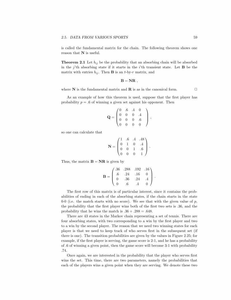
2.5. DATA FROM VARIOUS SPORTS 59
is called the fundamental matrix for the chain. The following theorem shows onereason that N is useful.
Theorem 2.1 Let bij be the probability that an absorbing chain will be absorbedin the j’th absorbing state if it starts in the i’th transient state. Let B be thematrix with entries bij . Then B is an t-by-r matrix, and
B = NR ,
where N is the fundamental matrix and R is as in the canonical form. 2
As an example of how this theorem is used, suppose that the first player hasprobability p = .6 of winning a given set against his opponent. Then
Q =
0 .6 .4 00 0 0 .40 0 0 .60 0 0 0
,
so one can calculate that
N =
1 .6 .4 .480 1 0 .40 0 1 .60 0 0 1
.
Thus, the matrix B = NR is given by
B =
.36 .288 .192 .16.6 .24 .16 00 .36 .24 .40 .6 .4 0
.
The first row of this matrix is of particular interest, since it contains the prob-abilities of ending in each of the absorbing states, if the chain starts in the state0-0 (i.e. the match starts with no score). We see that with the given value of p,the probability that the first player wins both of the first two sets is .36, and theprobability that he wins the match is .36 + .288 = .648.
There are 43 states in the Markov chain representing a set of tennis. There arefour absorbing states, with two corresponding to a win by the first player and twoto a win by the second player. The reason that we need two winning states for eachplayer is that we need to keep track of who serves first in the subsequent set (ifthere is one). The transition probabilities are given by the values in Figure 2.25; forexample, if the first player is serving, the game score is 2-1, and he has a probabilityof .6 of winning a given point, then the game score will become 3-1 with probability.74.
Once again, we are interested in the probability that the player who serves firstwins the set. This time, there are two parameters, namely the probabilities thateach of the players wins a given point when they are serving. We denote these two

60 CHAPTER 2. STREAKS
0 0.2 0.4 0.6 0.8Point probability
0.2
0.4
0.6
0.8
1Set
probability
Figure 2.27: Set-winning probabilities for players of equal abilities.
parameters by p1 and p2. If we let p1 = p2, then Figure 2.27 shows the probabilitythat the first player wins the set as a function of p1.
There is nothing very remarkable about this graph. Suppose instead that p1 =p2 + .1, i.e. the first player is somewhat better than the second player. In this case,Figure 2.28 shows the probability that the first player wins the set as a function ofp1 (given that the first player serves the first game). If, for example, p1 = .55 andp2 = .45, then the probability that the first player wins the set is .65.
Finally, suppose that two players play a best-of-three set match. The Markovchain corresponding to this situation has 11 states, because we must keep trackof who begins serving each set. Suppose that the first player has probability p
of winning a given point on his serve, and his opponent has probability p − .1 ofwinning a given point on his serve. Figure 2.29 shows the probability that the firstplayer will win the match as a function of p. Note that even though there is a dipin the graph, the probability that the first player wins the match is always at least.9, even though the probability that he wins a given point is only slightly greaterthan his opponent’s probability. What kind of streakiness, if any, is evident inprofessional tennis? The above models show that even with slight differences in theplayers’ abilities, many of the matches are likely to be one-sided. One can turn thisaround and say that the fact that there are so many close matches among the topprofessional tennis players means that these players must be very close in ability.
In [8], Jackson and Mosurski describe two models, and some variations on thesemodels, that deal with match scores in tennis. They were interested in the apparentoverabundance of ‘heavy defeats’ in tennis matches, i.e. best-of-three matches inwhich the loser does not win a set, or best-of-five matches in which the loser wins0 or 1 sets.
One can model the sequence of sets in a tennis match in several ways. Thesimplest model is a Bernoulli trials model, in which a given player has the same

2.5. DATA FROM VARIOUS SPORTS 61
0 0.2 0.4 0.6 0.8Point probability
0.2
0.4
0.6
0.8
1
Set
probability
Figure 2.28: Set-winning probabilities for players of unequal abilities.
0.5 0.6 0.7 0.8 0.9Point probability of first player
0.92
0.94
0.96
0.98
1
Match
probability
Figure 2.29: Match-winning probabilities for players of unequal abilities.

62 CHAPTER 2. STREAKS
0 50 100 150 200 250 300Rank difference
0
0.2
0.4
0.6
0.8
1Probability
of
winning
Figure 2.30: Observed winning probabilities vs. rank difference in 2002.
probability p of winning each set. In Exercise 1, we ask the reader to determine thedistribution of match scores under this assumption. In order to see if this modeldoes a good job of explaining the data, we need to have some way of estimatingp, since we certainly do not assume, even among professional tennis players, thatp = .5.
A reasonable way to proceed is to use the rankings of the players to estimate p.Tennis rankings of professional players are determined by the players’ performancein the previous twelve months. These rankings are updated each week. They arenot perfect because, for example, if a very good player is injured and doesn’t playfor awhile, his ranking can change by quite a bit, even though once he has recovered,he is presumably as good as he was before the injury.
We have obtained data from the website www.stevegtennis.com. We very muchappreciate the work that was done to create the raw data files that we used. Ourdata set consists of all men’s singles matches on the professional tour between 2000and 2002.
There are at least two ways to use player rankings to estimate p. One idea is tofit the observed probabilities to the difference of the two players’ ranks. A plot ofthe observed probabilities for the first sets in mens’ singles matches in 2002 versusthe difference in the ranks of the two players is shown in Figure 2.30. We onlyshow the results of matches where the rank difference was at most 300, since thereare comparatively few matches for each difference larger than this. There are 3925matches in the resulting data set. This figure also shows a best fit line. The readercan see that the fit is not very good; in fact, the correlation coefficient is .0298.
Jackson and Mosurski adopt a different strategy for estimating p. Denote byr and s the two players’ ranks, and assume that r ≤ s. They then define O(r, s)to be the odds (not the probability) that the better player wins the first set. Thereason that they define these odds in terms of the first set, rather than the match,

2.5. DATA FROM VARIOUS SPORTS 63
0 1 2 3 4 5 6 7Rank ratio
0.2
0.4
0.6
0.8
1
Prob.
of
winning
Figure 2.31: Observed winning probabilities vs. rank ratio in 2000-2002.
is that they are concerned about the outcomes of sets affecting the outcomes oflater sets in the same match. If we are considering a model in which the sets areconsidered to be independent events, then we can use O(r, s) as the odds that thebetter player wins any given set in the match. However, we must be careful withour use of O(r, s) if we are not assuming the sets are independent.
They next state the following assumed relationship among O(r, s), r and s:
O(r, s) = (ratio of ranks)α =(
s
r
)α
.
The parameter α is to be determined by the data. The above relation is equivalentto the relation
log(O(r, s)) = log(odds of success) = α log(s/r) .
This is a line through the origin with slope α.We carry out this regression for all matches in the years 2000 through 2002
in which the ratio of the ranks of the players is at most 7.4 (this is a completelyarbitrary cut-off; it is about e2). There were 12608 matches in this data set. Weobtain a value of α = .480, and a correlation coefficient of .363. Figure 2.31 showsthe observed probability of winning the match versus the ratio of the ranks, togetherwith the graph of the function (ratio)α.
Now that we have a way to estimate the probability that a given player will winthe first set against a certain opponent, we can proceed in several directions. First,we can explain and test the model of Jackson and Mosurski, which they call theodds model. Second, we can test for independence among the sets in professionaltennis matches.
In the odds model, it is assumed that the odds the better player will win a givenset depend upon the set score of the match. We let Oij denote the odds that the
64 CHAPTER 2. STREAKS
better will player will win the next set if the set score is i (for the better player) toj. The discussion above gives us an estimate for O00. The model asserts that eachtime a player wins a set, the odds for the next set change (in one direction or theother) by a factor of k, where k is to be determined by the data. So, for example, ifthe better player wins the first set, then the odds that he wins the second set equalkO00. In general, we have
Oij = ki−jO00 .
Using our estimate for O00, and taking logarithms, we have
log(Oij) = α log(s/r) + (i− j) log(k) .
Note that if we take k = 1, then we have the model where the sets are assumed tobe independent.
The above equation can be used, along with the data, to estimate α and k. Theprocedure we now describe results in the maximum likelihood estimates for α andk. In a nutshell, a maximum likelihood estimate for a set of parameters is the setof values for those parameters that leads to the highest probability for the data set.As an example of this idea, suppose that we flip a coin 20 times and observe 12heads. We wish to find the maximum likelihood estimate for p, the probability ofa head on a single toss. We certainly hope that this estimate is 12/20. Let us seeif this is the case. For each p between 0 and 1, we compute the probability that ifa coin has probability p of coming up heads, it will come up heads 12 times in 20tosses. This probability is (
2012
)p12(1− p)8 .
We wish to maximize this expression over all p. If we denote this expression byf(p), then we have
f ′(p) =(
2012
)(12p11(1− p)8 − 8p12(1− p)7
).
Setting this equal to 0 and solving for p, we obtain
p =1220
,
as we hoped. (It is easy to check that this value of p corresponds to a maximumvalue of f(p).) To reiterate, this means that the probability that we would actuallyobtain 12 heads in 20 tosses is largest if p = 12/20.
In the case of set scores in tennis, we treat each match as an independent event,and use the relationship given above among the odds that the better player winsa given set, α, and k, to compute the probability that we would obtain the actualdata set. Since the matches are assumed to be independent, this probability is theproduct of the probability that each match in the data set occurs, given valuesof α and k. This calculation is easy to carry out with a computer. The numberof completed best-of-three set matches in our data set is 12608. The maximumlikelihood estimates for the parameters are
α = .37

2.5. DATA FROM VARIOUS SPORTS 65
andk = 1.78 .
Note that this value of α is quite a bit different than the one we obtained using justthe first sets of the matches.
Now that we have estimated α and k, we can proceed, as in [8], to see how wellthe model fits the observed distribution of set scores in our data. The way thatwe do this is to simulate the matches many time on a computer, using the actualpairs of rankings in each match in the data set. When we did this 100 times, thedistribution of match results was
5271.77, 1196.99, 881.01, 941.8, 1317.93, 2998.5 ,
where the i’th number in the above list is the number of matches whose set out-comes (from the point of view of the better player) matched the i’th element in thefollowing list:
1, 1, 1, 0, 1, 1, 0, 0, 0, 1, 0, 0, 1, 1, 0, 0 .
This simulation gives us a decent approximation to the theoretical distribution. Tosee how well the model fits the actual distribution, we use a chi-squared test. Theactual distribution of the data is
5453, 1157, 993, 813, 1338, 2854 .
If we let Ei denote the i’th value in the theoretical distribution, and Oi denote thei’th value in the actual distribution, then value of the expression
6∑i=1
(Oi − Ei)2
Ei
is approximately chi-squared distributed with 5 degrees of freedom (see [7] for ex-amples of this technique). The value of the above expression is 46.69, which has ap-value of less than .01. So the model does not fit the data very well.
We can also carry out the above calculations under the assumption of indepen-dence of sets. To do this, we simply assume that the odds, O00, of the better playerwinning the first set continue to hold for all subsequent sets in the same match. Thiscorresponds to letting k = 1. However, we must re-estimate α, since our maximumlikelihood estimate of α was found simultaneously with our maximum likelihoodestimate of k. When we do this, we find a new estimate: α = .41. Using this value,and simulating the resulting distribution, we obtain the following approximation:
4459.56, 1742.79, 1235.17, 1241.94, 1746.56, 2181.98 .
The chi-squared value in this case is 916.374, which is much larger than in theprevious case. So we might conclude that the odds model fits the data better thanthe independent set model, but neither fits the data well.

66 CHAPTER 2. STREAKS
Before moving to the best-of-five set data, we digress slightly to suggest anotherway to estimate α and k. This method involves minimizing the value of the chi-squared distribution. More precisely, we try to find the values of α and k so thatwhen the theoretical values of the distribution are compared with the actual values,the chi-squared value is as small as possible. This method is due to Karl Pearson,who was the originator of the chi-squared method of comparing distributions.
The values of α and k that minimize the value of the chi-squared distributionfor the best-of-three set matches are .41 and 1.75, which we note are very close tothe maximum likelihood estimates for these parameters. For these values of α andk, the p-value of the observation is still less than .01, once again signifying that thefit is not good.
When we repeat the maximum likelihood calculations for all of the best-of-fiveset matches played between 2000 and 2002, the fit of the odds model is much better.There were 1571 completed best-of-five set matches in the data set. The maximumlikelihood estimates for α and k are .31 and 1.51. The chi-squared value of theobservation is 17.54, with a p-value of .55. We use a chi-squared distribution with19 degrees of freedom, since there are 20 possible outcomes in a best-of-five setmatch.
If we attempt to fit the independent set model to the data, we find a maximumlikelihood estimate for α of .36, and a chi-squared value of 235.2. The p-value forthis observation is less than .01. Thus the odds model fits the data fairly well, anddoes a much better job than the independent set model.
There is another way to help us decide whether professional tennis matchesare streaky. Consider a best-of-three set match. If each player has won one setin the match, then we might think that they are equally likely to win the third,and deciding, set. Of the 12608 completed best-of-three set matches in our dataset, 4301 required three sets to complete. Of these 4301 matches, 2331 matcheswere won by the player who won the second set. Thus, among the matches thattook three sets to complete, if a player won the second set, the probability that hewon the third set is .542. If the sets were independent, we might think that thisprobability should be close to .5. Since the actual probability is greater than .5,one could say that the player who won the second set has ‘momentum’, or is ‘ona streak.’ Before concluding that this is evidence of streaky behavior, we shouldconsider the relative abilities of the players involved in the matches. It is possiblethat the reason that the winner of the second set does so well in the third set isbecause he is the better player.
If we simulate a distribution of set scores, using the value of α = .480 (obtainedearlier by fitting the odds model to just the first sets in the matches in the data), weobtain the following (the average of 20 simulations, using the same sets of opponentsas in the actual data set):
4676.65, 1740.05, 1187.75, 1180.4, 1746.85, 2076.3 .
In this simulated distribution, there are 5855 matches that took three sets to com-plete. In these matches, there were 2935 (which is almost exactly one-half of 5855)

2.6. ADAPTIVE THINKING 67
in which the player who won the second set won the third. Thus, we can discountany effect due to the relative ranks of the players.
It is also the case that this percentage does not change very much if we varyα. For α = .3, .31, . . . , .5, the percentage stays between .497 and .505. Thus, wemay assume that in this model, the player who won the second set has about a 50%chance of winning the third set.
How likely is it that in as many as 2331 matches out of 4301, the player who winsthe second set wins the third set as well, given our assumption about independenceof sets? This is essentially the same question as asking how likely a fair coin, iftossed 4301 times, will come up heads at least 2331 times. The number of heads ina long sequence of coin flips is approximately normal. If the coin is fair, and thenumber of tosses is n, then the mean is n/2 and the standard deviation is
√n/2.
The standardized value corresponding to 2331 is
2331− n/2√n/2
= 5.505 .
The probability that a standard normal random variable takes on a value greaterthan 5.505 is much less than .01. Thus, we can claim that the data exhibits streak-iness.
Exercises
1 Assume that two players are playing a best-of-three set tennis match, and thefirst player has probability p of winning each set (i.e. the sets are independenttrials). Find the distribution of the four possible match outcomes: 2-0, 2-1,1-2, and 0-2.
2.6 Adaptive Thinking
2.7 Runs in the Stock Market
It is accepted that over the long run, most stocks go up in price. Thus, one way tomodel the price of a stock is to imagine that there is a line, with positive slope, thatrepresents the long-term trend of the stock, and then consider the stock’s variationabout this line. It is typically the case that instead of using the daily prices of thestock, one uses the logarithms of these prices. In this case, a straight trend linecorresponds to the stock price changing by a constant percentage each day. Theslope of the trend line can be found by either fitting a straight line to the log pricedata, or simply by using the starting and ending points of the data as anchor pointsfor the line. In either case, the slope cannot be found unless one knows the data.
As might be imagined, an incredible amount of effort has been directed to theproblem of modeling stock prices. In Chapter 4, we will focus on what is knownabout the distribution of the residual movements (those that remain after the trendline has been subtracted from the data) of stock prices. In this section, we will
68 CHAPTER 2. STREAKS
consider whether the stock market exhibits streaky behavior (or perhaps other formsof non-randomness).
One obvious way in which stock prices could be streaky concerns their dailyup-and-down motions. Most stocks have more up days than down days, so onemight model them with coins whose success probabilities are greater than .5. Usingthe data, one can compute the observed success probability, and then count thenumber of success (or failure) streaks of a given length, or of any length. Then onecan compare these observed values with the theoretical values.
Our data set consists of daily prices of 439 of the stocks that make up the S&P500 list. These prices have been adjusted to take into account dividends and stocksplits. For this reason, many of the stock prices are very small near the beginningof the data set, and hence are subject to rounding errors. We typically get aroundthis problem by using only the part of the data set in which a stock’s price is abovesome cutoff value. Also, we throw out all days for a given stock on which the stockprice was unchanged.
Suppose that we want to compare the expected and the observed number ofpairs of consecutive days in which a given stock’s price went up on both days. Ifwe have n data points, then we can define the random variable Xi to equal 1 ifthe i’th and (i + 1)’st price changes are both positive, and 0 otherwise. Under theassumption that the signs of the daily price changes are independent events, theprobability that Xi = 1 is just p2, where p is the observed long-range probability ofsuccess for that stock. Thus, it is easy to calculate the expected number of up-uppairs. There are n − 1 daily changes (since there are n data points), so there aren − 2 random variables Xi, each with the same distribution. Thus, the expectednumber of up-up pairs is just
(n− 2)p2 .
Unfortunately, the Xi’s are not mutually independent. For example, if X6 = 1and X8 = 1, then it is not possible for X7 to equal 0. Nonetheless, the Xi’s arem-independent, for m = 2. This concept means that it is possible to partitionthe sequence Xi into m subsets such that the random variables in each subsetare mutually independent. In this case, we can use the partition X1, X3, . . . andX2, X4, . . .. If a sequence of random variables is m-independent, then it satisfiesa modified version of the Central Limit Theorem. (The modification comes in howthe variance of the sum of the random variables is calculated.)
Using this modified version of the Central Limit Theorem, we can transform thesum X1 + X2 + . . . + Xn−1 into a random variable that is approximately standardnormal (this is done in the usual way; we subtract the mean and divide by thestandard deviation). This gives us, for each stock, a z-value, i.e. a value of astandard normal distribution that represents how far above or below the mean theobserved number of up-up pairs is. This approach works for any other pattern, suchas down-down, or up-down-up, etc.
If stocks are streaky, then the z-values for up-up pairs (and for down-down pairs)should be significantly greater than 0. The same thing should be true for up-up-uptriples. For each of several different patterns, we calculated the set of z-values forall 439 stocks in our data set. We used 1 as our cutoff value, meaning that for each
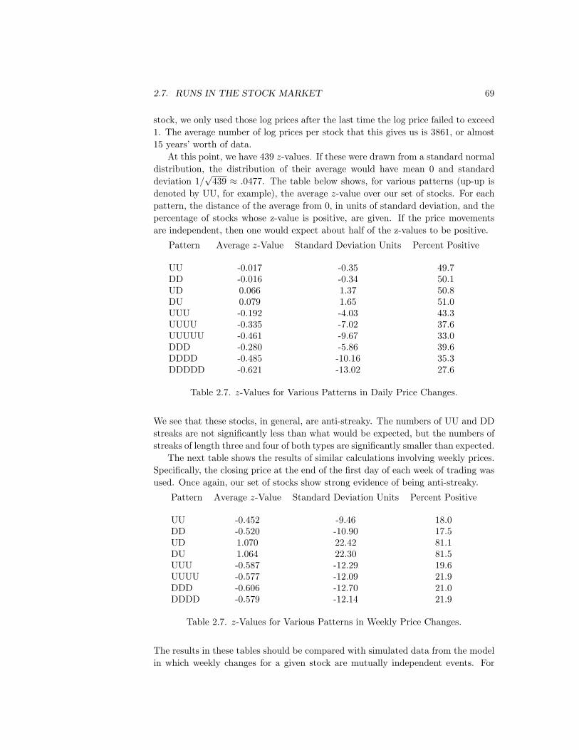
2.7. RUNS IN THE STOCK MARKET 69
stock, we only used those log prices after the last time the log price failed to exceed1. The average number of log prices per stock that this gives us is 3861, or almost15 years’ worth of data.
At this point, we have 439 z-values. If these were drawn from a standard normaldistribution, the distribution of their average would have mean 0 and standarddeviation 1/
√439 ≈ .0477. The table below shows, for various patterns (up-up is
denoted by UU, for example), the average z-value over our set of stocks. For eachpattern, the distance of the average from 0, in units of standard deviation, and thepercentage of stocks whose z-value is positive, are given. If the price movementsare independent, then one would expect about half of the z-values to be positive.
Pattern Average z-Value Standard Deviation Units Percent Positive
UU -0.017 -0.35 49.7DD -0.016 -0.34 50.1UD 0.066 1.37 50.8DU 0.079 1.65 51.0UUU -0.192 -4.03 43.3UUUU -0.335 -7.02 37.6UUUUU -0.461 -9.67 33.0DDD -0.280 -5.86 39.6DDDD -0.485 -10.16 35.3DDDDD -0.621 -13.02 27.6
Table 2.7. z-Values for Various Patterns in Daily Price Changes.
We see that these stocks, in general, are anti-streaky. The numbers of UU and DDstreaks are not significantly less than what would be expected, but the numbers ofstreaks of length three and four of both types are significantly smaller than expected.
The next table shows the results of similar calculations involving weekly prices.Specifically, the closing price at the end of the first day of each week of trading wasused. Once again, our set of stocks show strong evidence of being anti-streaky.
Pattern Average z-Value Standard Deviation Units Percent Positive
UU -0.452 -9.46 18.0DD -0.520 -10.90 17.5UD 1.070 22.42 81.1DU 1.064 22.30 81.5UUU -0.587 -12.29 19.6UUUU -0.577 -12.09 21.9DDD -0.606 -12.70 21.0DDDD -0.579 -12.14 21.9
Table 2.7. z-Values for Various Patterns in Weekly Price Changes.
The results in these tables should be compared with simulated data from the modelin which weekly changes for a given stock are mutually independent events. For

70 CHAPTER 2. STREAKS
each stock in our set, we used the observed probabilities of a positive and a negativeweekly change in the stock price to create a simulated set of stock prices. Then,using the same algorithms as were used above, we calculated the average z-valuesfor various patterns over our set of stocks. The results are shown in the table below.
Pattern Average z-Value Standard Deviation Units Percent Positive
UU -0.010 -0.21 50.1DD -0.074 1.56 51.7UD 0.005 0.10 51.0DU 0.002 0.04 51.0UUU -0.035 -0.74 44.9UUUU -0.020 -0.41 46.2DDD 0.064 1.34 50.8DDDD -0.060 -1.26 43.7
Table 2.7. Simulated z-Values for Various Patterns in Weekly Price Changes.
The simulated data from this model is much different than the actual data. Thissupports the observation that both daily and weekly stock prices are anti-streaky.
In their book[11], Andrew Lo and Craig MacKinlay discuss a parameter theycall the variance ratio. Suppose that Xin
i=0 is a sequence of n logarithms ofa stock’s price. The time increment between successive values might be days, orweeks, or even something as small as minutes. The log price increments are thevalues Xi+1 −Xin−1
i=0 . A central question that concerns this sequence of log priceincrements is whether it can be modeled well by a process in which the incrementsare assumed to be mutually independent.
Lo and MacKinlay begin by fixing a stock and a sequence of log prices Xini=0
for that stock. All prices have been adjusted for splits and dividends, and weassume in what follows that the time increment is a week. Next, they calculate theestimator
µ =1n
n−1∑i=0
(Xi+1 −Xi
),
which is an estimate of the average change per week in the logarithm of the stockprice. This expression can be simplified to
µ =1n
(Xn −X0
).
Next, they calculate the estimator
σ2 =1n
n−1∑i=0
(Xi+1 −Xi − µ
)2,
which is an estimator of the variance of the weekly change in the logarithm of thestock price. If we assume for the moment that n is even, we could instead look at

2.7. RUNS IN THE STOCK MARKET 71
the estimator1
n/2
n−1∑i=0
(X2i+2 −X2i − 2µ
)2,
which is an estimator of the variance of the increments in even-numbered observa-tions. Under the assumption that the increments are independent, the variance ofthe differences
X2i+2 −X2i
is twice the variance σ2 of the differences
Xi+1 −Xi .
This provides a way to test whether the assumption of independent increments instock prices is a reasonable one. One can compute both estimators for a given stock,and see how close the ratio is to two.
Lo and MacKinlay slightly change the second variance estimator above, by di-viding by two. So let us define
σ22 =
1n
(n−1)/2∑i=0
(X2i+2 −X2i − 2µ
)2.
Under the assumption of independent increments, the theoretical value of σ22 (for
which σ22 is an estimator) equals the value of σ2. Thus, still under this assumption,
the ratio of the estimators should be close to 1. Of course, one can, for any integerq > 1, define the estimator σq
2 in the same way. Once again, under the assumptionof independent increments, σ2
q = σ2.Lo and MacKinlay modify the above set-up in one additional way. Instead of
using non-overlapping time increments in the definition of σq2, they use all of the
time increments of length q, obtaining the following definition (note that we nolonger need to assume that q divides n):
σq2 =
1q(n− q + 1)
(n−q+1)∑i=0
(Xi+q−1 −Xi − qµ)2 .
The test statistic for the variance ratio σq2/σ2 is denoted by Mr(q) (the subscript
refers to the fact that we are dealing with a ratio), and is defined by
Mr(q) =σq
2
σ2− 1 .
We have seen that under the assumption of independent increments, this statisticshould typically be close to 0. In order for it to be a useful statistic in testingthis assumption, we need to know something about how this statistic is distributed.Lo and MacKinlay show that for large n, the statistic
√nMr(q) is approximately
normally distributed with mean 0 and variance
2(2q − 1)(q − 1)3q
.

72 CHAPTER 2. STREAKS
(In fact, to be strictly accurate, they make one further modification, that we willignore, in order that the estimators are unbiased. The above asymptotic statementdoes not change when this modification is made.)
Lo and MacKinlay calculated the variance ratio for both individual stocks andfor various sets of stocks on the New York and American stock exchanges. Theirdata consisted of weekly prices for 625 stocks from 1962 to 1985 (1216 weeks). Forthe values q = 2, 4, 8, and 16, their observed values of Mr(q) for the set of all stocksin their data set were .30, .64, .94, and 1.05 respectively. These were all statisticallydifferent from 0 at the 5% level of significance.
They also computed the average variance ratio for the individual stocks. For theabove values of q, these average variance ratios were −.03,−.06,−.08, and −.11.These observed values were not statistically different from 0 at the 5% level ofsignificance. However, it is interesting that these observed values are all of oppositesign from those corresponding to the set of all stocks.
It is possible to describe a situation in which the variance ratio of a stock (forq = 2, say) would be negative. Suppose that over blocks of two consecutive weeks,there were more up-down and down-up pairs than expected. This might meanthat the average net change in the stock’s price over two-week periods might besomewhat less than twice the average net change over one-week periods, and thesame might be true of the average variance.
The above is admittedly only speculation. We carried out two sets of calculationswith our stocks to see if any of this speculation is correct. First, we calculated thevariance ratios for our stocks, for the values of q listed above. The average varianceratios were -.060, -.103, -.135, and -.159.
Our second set of calculations consisted of simulating our stocks by using atwo-state Markov chain, in which the transition matrix entries are obtained fromthe observed probabilities for the four possible pairs up-up, up-down, down-up, anddown-down (these were discussed above). For each of the above q, we simulatedeach of our stocks ten times, and computed the average variance ratio. Then wecomputed the average, over all of the stocks, of these averages. The values obtainedwere -.088, -.125, -.142, and -.153. Furthermore, of the 439 stocks, the numberswhose average simulated variance ratio had the same sign as the actual varianceratio, for q = 2, 4, 8, and 16, were 386, 384, 373, and 358. So the Markov chainmodel behaves similarly, in terms of the variance ratio, to the actual stock prices.
2.8 Conclusions
2.9 Appendix
In this section, we will show how one can use generating functions to derive thetheoretical distributions of several parameters of interest in this chapter. The dis-tribution of the number of runs in a sequence of n Bernoulli trials was calculatedby Mood [12]. An example of this distribution, with n = 50 and p = .2, is shown inFigure 2.1.
2.9. APPENDIX 73
One sees two roughly normal-shaped distributions. The reason for this is thatthe probability that the number of runs is even does not equal the probability thatthe number of runs is odd (except if p = 1/2). In fact, the number of runs iseven if and only if the first trial and the last trial disagree, which happens withprobability 2p(1 − p). Thus, the sum of the distribution values corresponding toeven-valued outcomes equals this value, and the odd distribution values sum to 1minus this value. (Note to us: This picture means that it might be better to workwith the number of success runs.) We will give a derivation of this distribution thatis different than the one found in [12], using a method that will generalize to thedistribution of the number of success runs (i.e. the number of runs in the first state)of a Markov chain with two states. The distribution was first derived by Zaharovand Sarmanov [16].
If we denote by rn,k the probability of k runs in n trials (this number alsodepends upon p), then we will show that the generating function
r(x, y, p) =∞∑
n=1
n∑k=1
rn,kxnyk
equalsxy(1 + 2px(−1 + y)− 2p2x(−1 + y))
1− x + (−1 + p)px2(−1 + y2).
To derive this expression, we start by defining f(n, p, k, S) to be the probabilitythat in a sequence of n Bernoulli trials with success probability p, there are exactlyk runs and the sequence ends in a success. The quantity f(n, p, k, F ) is definedsimilarly. Next, we define
G(x, y) =∞∑
i=1
i∑j=1
f(i, p, j, S)xiyj
and
H(x, y) =∞∑
i=1
i∑j=1
f(i, p, j, F )xiyj .
How are the coefficients related to one another? If a sequence of length at least twoends in a success, and it has k runs, and we chop off the last term in the sequence,we obtain a sequence of length n− 1 that still has k runs and ends in a success, orit has k − 1 runs and ends in a failure. Thus, for n ≥ 2, we have
f(n, p, k, S) = f(n− 1, p, k, S)p + f(n− 1, p, k − 1, F )q .
Similarly, we have, for n ≥ 2,
f(n, p, k, F ) = f(n− 1, p, k, F )q + f(n− 1, p, k − 1, S)p .
These recursions do not hold when n = 1, because f is not defined if the firstparameter is 0. When n = 1, we have
f(1, p, 1, S) = p
74 CHAPTER 2. STREAKS
andf(1, p, 1, F ) = q .
Using the recursions and initial conditions given above, we can write
G(x, y) = pxyH(x, y) + pxG(x, y) + pxy ,
andH(x, y) = qxyG(x, y) + qxH(x, y) + qxy .
One can solve these equations for G(x, y) and H(x, y), obtaining
G(x, y) =pxy(1 + x(−1 + p + y − py))
1− x + (pqx2(1− y2)
and
H(x, y) =(−1 + p)xy(1 + px(−1 + y))
1− x + (pqx2(1− y2).
Finally, note thatr(n, k) = f(n, p, k, S) + f(n, p, k, F ) ,
sor(x, y, p) = G(x, y) + H(x, y) ,
giving us the required expression for r(x, y, p).The above expression for the generating function r(x, y, p) allows one to write
an exact expression for rn,k. The expression for r(x, y, p) is of the form
xyA + Bx
C + Dx + Ex2
where the capital letters represent expressions that do not involve x. Using the alge-braic method of partial fractions (usually first learned in calculus to help integraterational functions), one can write this expression as
xy
(F
1−Gx+
H
1− Ix
).
The two summands can be rewritten, using ideas about geometric series, to obtain
xy(F + FGx + FG2x2 + . . . + H + HIx + HI2x2 + . . .) .
We want the coefficient of xnyk in this expression. The coefficient of xn is
y(FGn−1 + HIn−1) .
This is a series involving y but not x. We want the coefficient of yk in this series.The answer, which is obtained after some gruesome algebra (best performed by acomputer algebra package) is as follows. Let q = 1− p. If k is odd, then
rn,k =1
2n−1
[ bn2 c∑
j=(k−1)
2
(n
2j + 1
) j∑i=
(k−1)2
(j
i
)(4pq)i
(i
(k − 1)/2
)(−1)i−(k−1)/2
−4pq
bn−12 c∑
j=(k−2)
2
(n− 12j + 1
) j∑i=
(k−1)2
(j
i
)(4pq)i
(i
(k − 1)/2
)(−1)i−(k−1)/2
],

2.9. APPENDIX 75
while if k is even, then
rn,k =4pq
2n−1
bn−12 c∑
j= k2
(n− 12j + 1
) j∑i=
(k−2)2
(j
i
)(4pq)i
(i
(k − 2)/2
)(−1)i−(k−2)/2 .
These expressions were used to generate Figure 2.1.We can use the expression for r(x, y, p) to calculate the mean (and variance)
of the distribution. We recall that for fixed n, the mean of the distribution rn,kequals
n∑k=1
krn,k .
The value of this sum can be obtained from the generating function r(x, y, p) byusing calculus. If we compute the partial of r(x, y, p) with respect to y, and thenset y = 1, we obtain the expression
∞∑n=1
n∑k=1
krn,kxn ,
which can be written as∞∑
n=1
xnn∑
k=1
krn,k .
Thus the mean of the distribution for sequences of length n is just the coefficientof xn in the above expression. The point of this is that we do not need to use theformulas for rn,k to calculate the mean. Rather, we use the closed-form expressionfor r(x, y, p), and apply the ideas above to this expression.
If we perform these calculations, we obtain the expression
x
1− x+
2pqx3
(1− x)2+
2pqx2
1− x.
Using the facts that1
1− x= 1 + x + x2 + . . .
and1
(1− x)2= 1 + 2x + 3x2 + . . . ,
in a suitable interval containing the origin, we can expand each of the three sum-mands above as series; they are, respectively,
x + x2 + x3 + . . . ,
2pq(x3 + 2x4 + 3x5 + . . .) ,
and2pq(x2 + x3 + x4 + . . .) .

76 CHAPTER 2. STREAKS
Now we can easily write down the coefficient of xn; it is
1 + 2pq(n− 2) + 2pq = 1 + 2pq(n− 1) ,
if n ≥ 2.There is an easy way to check this. In fact, the calculation below is an easier
way to find the mean in this case, but the above method can be used to find othermoments (including the variance) and the calculation below does not generalize.Let Xi, for 1 ≤ i ≤ n − 1, denote the random variable that is 1 if the i’th and(i + 1)’st outcomes disagree. Then the average number of runs is just
n−1∑i=1
Xi ,
so
µ =n−1∑i=1
E(Xi) .
But for each i, the probability that Xi = 1 is just 2pq, so for each i,
E(Xi) = 2pq ,
so the average number of runs is just
= 1 + 2p(1− p)(n− 1) .
In the Markov model, the situation is more complicated(!). We will not go intothe details here, but rather give an outline of how to proceed. We write
fS,S(n, k)
for the probability that a sequence of n trials begins and ends with a success andhas k runs. The quantities fS,F , fF,S and fF,F are defined similarly. We define thegenerating function
GS,S(x, y) =∞∑
n=1
∞∑k=1
fS,S(n, k)xnyk ;
the functions GS,F , GF,S , and GF,F are defined in a similar manner. One can showthat
GS,S(x, y) = p2xyGS,F (x, y) + p1xGS,S(x, y) + xy ,
GS,F (x, y) = (1− p1)xtGS,S(x, y) + (1− p2)xGS,F (x, y) ,
GF,S(x, y) = p2xyGF,F (x, y) + p1xGS,F (x, y) ,
GF,F (x, y) = (1− p1)xyGS,F (x, y) + (1− p2)xGF,F (x, y) + xy .
Note that two of these equations are homogeneous (there are no summands onthe right-hand sides that do not involve the functions G∗,∗) which makes it easyto find GS,F , say, once we have found GS,S . In addition, by switching the roles of

2.9. APPENDIX 77
success and failure, one sees that it is easy to find GF,F once we know GS,S (andGF,S once we know GS,F ).
Thus, we only need to find the coefficients fS,S(n, k), in a manner similar to theone used to obtain the results for Bernoulli trials. One can show that
GS,S(x, y) =xy
1− (p2(1− p1)x2y2)/(1− (1− p2)x)− p1x.
Note that since the sequences corresponding to GS,S(x, y) begin and end with asuccess, the only positive probabilities are those corresponding to odd k. If k isodd, then
fS,S(n, k) =1
2n−1
[(−(1− p1 − p2)
b (n−2)2 c∑
j=0
(n− 12j + 1
)(1 + p1 − p2)n−1−(2j+1)
(
j∑i= k−1
2
(j
i
)(1+p1−p2)2(j−i)(−4)i(−((1−p1)p2))(k−1)/2(p1(1−p2))i−(k−1)/2
(i
(k − 1)/2
))
+bn−1
2 c∑j=0
(n− 1
2j
)(1 + p1 − p2)n−1−2j
(j∑
i= k−12
(j
i
)(1+p1−p2)2(j−i)(−4)i(−((1−p1)p2))(k−1)/2(p1(1−p2))i−(k−1)/2
(i
(k − 1)/2
))⌋.
One can use the recursions relating GS,S(x, y) and GS,F (x, y) given above to obtainthe following formula for fS,F (n, k):
fS,F (n, k) = (1− p1)n−1∑l=0
(1− p2)lfS,S(n− l − 1, k − 1) .
These formulas are useful in plotting the distributions (depending upon whetherthe first trial is a success or a failure) of the number of runs. In Figure 2.2 a plot ofthe distribution for n = 50, p1 = .3, and p2 = .1, where the first trial is a success.
We note that the fixed probability vector of the transition matrix in the Markovchain model equals (
p2
1− p1 + p2,
1− p1
1− p1 + p2
).
This means that the long-term proportion of successes equals
p2
1− p1 + p2.
Note that in this model, we have three quantities that can be estimated from thedata, namely p1, p2, and the long-term proportion of successes (which we will callp), but there is a relation among them. I have no idea how a statistician would dealwith this, since it is unlikely that the observed values satisfy the relation.

78 CHAPTER 2. STREAKS
In order to create a distribution for the Markov chain model, we will weight thedistributions corresponding to starting with a success or a failure by p and (1− p).The resulting generating function is
p(GS,S(x, y) + GS,F (x, y)
)+ (1− p)
(GF,S(x, y) + GF,F (x, y)
).
If we do this, the expected number of runs equals
nΩ1 + pΩ2 + (1− p)Ω4 + (pΩ3 + (1− p)Ω5)(p1 − p2)n−1 ,
where
Ω1 =2p2(1− p1)1− p1 + p2
,
Ω2 =2− 4p1 + 2p2
1 − p2 + 3p1p2 − 2p21p2 − p2
2 + 2p1p22
(1− p1 + p2)2,
Ω3 =−1 + 2p1 − p2
1 + p2 − p1p2
(1− p1 + p2)2,
Ω4 =1− 2p1 + p2
1 − p2 + 3p1p2 − 2p21p2 + 2p1p
22
(1− p1 + p2)2,
Ω5 =p2(1− p1 − p2)(1− p1 + p2)2
.
Thus, the expected number of runs is asymptotic to
nΩ1 + Ω4 .
If one lets p1 = p2, so that the Bernoulli model is obtained, one can check that theresult agrees with the one already obtained.
The two graphs show what one might expect, namely that the expected numberof runs in the Markov model is less than in the Bernoulli trials model. It is easy toshow this; one need only show that if p1 > p2, then
Ω1 < 2p(1− p) .
Next, it might be nice to show that the runs distribution corresponding toGS,S(x, y) is asymptotically normal. One might need to do this to discuss thepower of the test that compares the two models.
We also might try writing approximation algorithms for the calculation of theseprobabilities, since the probabilities fall off rapidly and it is time-consuming tocalculate the sums using the exact expressions.
The distribution of the length of the longest success run in the Markov chainmodel can be calculated using recursions. Define A(n, x, k, p1, p2) to be the probabil-ity that a Markov sequence, beginning with a success, has no success run exceedingx in length, and ends with k successes, for 0 ≤ k ≤ x. This function satisfies thefollowing equations. First, if n = 1, then the function is 1 if k = 1 and 0 otherwise.If n > 1, then if k > 1,
A(n, x, k, p1, p2) = A(n− 1, x, k − 1, p1, p2)p1 ,
2.9. APPENDIX 79
since a sequence of length n that ends in k successes is obtained from one of lengthn−1 that ends in k−1 successes by adding one success to the end, and this happenswith probability p1, since k > 1. If n > 1 and k = 1, then
A(n, x, 1, p1, p2) = A(n− 1, x, 0, p1, p2)p2 ,
since in this case we are adding a success to the end of a sequence whose last statewas the failure state. Finally, if n > 1 and k = 0, then
A(n, x, 0, p1, p2) =( x∑
j=1
A(n−1, x, j, p1, p2)(1−p1))
+A(n−1, x, 0, p1, p2)(1−p2) ,
since in this case either there were j successes immediately preceding the last trial,which was a failure, for some j between 1 and x, or else the penultimate trial wasalso a failure.
These equations allow one to compute the values of the function A. To obtainthe desired distribution, namely the set of probabilities that a Markov sequence,beginning with a success, has longest success run exactly equal to x, we computethe quantity
x∑k=0
A(n, x, k, p1, p2)−x−1∑k=0
A(n, x− 1, k, p1, p2) .
This adds the weights of all of the sequences with longest success run at most x,and subtracts from this the weights of all of the sequences with longest success runat most x− 1.
2.9.1 Doubletons
We now turn to the question of the distribution of d, the number of doubletons (i.e.consecutive pairs of successes in a sequence of trials). The reason for our interestin this quantity is because, as was stated in Exercise 1, the number d is closelyrelated to p1, the probability of a success following a success, and p1 is of interestwhen studying autocorrelation. We will first consider asymptotic behavior of thedistribution of the number of doubletons, in both the Bernoulli trials model andthe Markov model, and then we will derive a recursion for the exact distribution inthe Bernoulli case.
Since the Bernoulli trials model is a special case of the Markov model, we willwork with the Markov model. In this model, the probabilities that a success followsa success or a failure are defined to be, respectively, p1 and p2.
We are interested in the distribution of d for large values of n, the length of thesequence. It turns out that if n is large, it does not matter very much in whichstate the Markov chain started (i.e. whether the first trial resulted in a success ora failure). We have stated above that the long-term fraction of the time that thechain is in state 1 is equal to
p2
1− p1 + p2.
Note that if p1 = p2 (i.e. we are in the Bernoulli model) then this expression reducesto p2 (= p1).

80 CHAPTER 2. STREAKS
We can find the distribution of the number of doubletons in a sequence of lengthn generated by the Markov process by considering the related Markov chain thatconsists of four states: SS, SF, FS, and FF. The first state, SS, means that thefirst two trials in the original sequence are both successes. It is straightforward todetermine the transition probabilities for this new Markov chain. For example, ifthe chain is in state SS, it stays in state SS or moves to state SF depending uponwhether the next trial in the original chain is a success or a failure. Thus,these twotransitions occur with probability p1 and moves to state SF with probability 1−p1.
In the new Markov chain, we wish to know the distribution of the numberof times Y
(n)SS that the chain is in state SS in the first n trials. Of course, this
distribution depends upon the starting state (or starting distribution), but it turnsout that the limiting distribution is independent of the starting state. The CentralLimit Theorem for Markov Chains (see [9], pg. 89) states that Y
(n)SS is asymptotically
normally distributed, with a mean and standard deviation that are straightforwardto calculate. Examples of how the mean and standard deviation are calculated aregiven in [9]. In the present case, the asymptotic value of the mean and standarddeviation are
np1p2
1− p1 + p2
andnp1p2(p2
1(−1 + p2) + (1 + p2)2 − p1p2(3 + p2))(1− p1 + p2)3
.
Now suppose that we have a process that presents us with a sequence of successesand failures, and suppose that the observed probability of a success is .3. We assumethat p = .3, and we wish to test the hypothesis that p1 = .3 against the alternativehypothesis that p1 > .3. To carry out this test, using the number of doubletons as aparameter, we first choose an acceptance region around the value np2 in which 95%of the values will fall (remember, in the case that the null hypothesis is true, thenp1 = p2 = p, and we are dealing with Bernolli trials). Since Y
(n)SS is asymptotically
normal, it is easy to pick this acceptance region. It is an interval of the form [0, c],because the form of the alternative hypothesis is a one-way inequality. The numberc is np2 plus 1.65 times the standard deviation of Y
(n)SS . We obtain the value of
c = n(.3)2 + 1.65√
.1197n .
This leads us to the distributions shown in Figures 2.4 to 2.5.We now give an outline of the method used to find the exact distribution of the
number of doubletons in the Bernoulli model, with parameters n and p. We definer(n, k, p) and s(n, k, p) to be the probabilities of exactly k doubleton successes inn trials, with success probability p, and with the sequence ending in a failure or asuccess, respectively. Then the following recursions hold:
r(n, k, p) = q ∗ r(n− 1, k, p) + q ∗ s(n− 1, k, p) ,
s(n, k, p) = p ∗ r(n− 1, k, p) + p ∗ s(n− 1, k − 1, p) .
The first of these equations says that sequences of length n with exactly k doubletonsand which end in a failure arise from sequences of length n − 1 with exactly k

2.9. APPENDIX 81
doubletons by adding a failure to the end. The second equation says that sequencesof length n with exactly k doubletons and which end in a success arise by adding asuccess to the end of either a sequence of length n − 1 with exactly k doubletons,ending in a failure, or to the end of a sequence of length n − 1 with exactly k − 1doubletons, ending in a success.
Next, define
R(p, x, y) =∞∑
n=1
n−1∑k=0
r(n, k, p)xnyk
and
S(p, x, y) =∞∑
n=1
n−1∑k=0
s(n, k, p)xnyk .
The distribution of the number of doubletons in sequences of length n is given bythe set of values
r(n, k, p) + s(n, k, p) .
The above recursions, together with attention to initial conditions, give rise tothe following functional equations:
R(p, x, y) = qx
(R(p, x, y) + S(p, x, y)
)+ qx
and
S(p, x, y) = px
(R(p, x, y) + S(p, x, y)
)+ px .
These equations can be solved for R(p, x, y) and S(p, x, y):
R(p, x, y) = −1 +1− pxy
1− qx− pqx2 − pxy + pqx2y
andS(p, x, y) =
px
1− qx− pqx2 − pxy + pqx2y,
where q = 1− p.We can write
1 + R(p, x, y) =A
1− γ1x+
B
1− γ2x,
for suitable choices of constants A, B, γ1, and γ2. The right-hand side can beexpanded to yield
(A + B) + (Aγ1 + Bγ2)x + (Aγ21 + Bγ2
2)x2 + . . . ,
allowing us to determine the coefficient of xn. A similar method allows us to dealwith S(p, x, y).
If we let∆ = q2 − 2pq(−2 + y) + p2y2 ,

82 CHAPTER 2. STREAKS
then one can show, after some work, that the coefficient of xn in the power seriesfor R(p, x, y) equals
12n
((q − py)
bn/2c∑j=0
(n
2j + 1
)(q + py)n−2j+1∆j +
bn/2c∑t=0
(q + py)n−2t∆t
),
and the coefficient of xn in the power series for S(p, x, y) equals
p
2n−1
bn/2c∑j=0
(n
2j + 1
)(q + py)n−2j−1∆j .
To obtain r(n, k, p) and s(n, k, p) from these expressions, we need to find thecoefficients of yk in the above expressions. Writing ∆j
l for the coefficient of yl in∆j , one can show that
∆jl =
l∑h=0
(j
h
)pl(−1)l(q − 2
√−pq)j−h(q + 2
√−pq)j−l+h .
Using this abbreviation, one can then show that
r(n, k, p) =12n
(q
bn/2c∑j=0
(n
2j + 1
) k∑l=0
∆jl
(n− 2j − 1
k − l
)pk−lqn−2j−1−(k−l)
−p
bn/2c∑j=0
(n
2j + 1
) k−1∑l=0
∆jl
(n− 2j − 1k − 1− l
)pk−1−lqn−2j−1−(k−1−l)
+bn/2c∑j=0
(n
2j
) k∑l=0
∆jl
(n− 2j
k − l
)pk−lqn−2j−(k−l) ,
)
and
s(n, k, p) =p
2n−1
bn/2c∑j=0
(n
2j + 1
) k∑l=0
∆jl
(n− 2j − 1
k − l
)pk−lqn−2j−1−(k−l) .
As before, we can use the closed-form expressions for R(p, x, y) and S(p, x, y) tofind the mean and variance of the distribution of the number of doubletons (andif we compare these expressions with the asymptotic ones obtained above for theMarkov case, we can partially check the accuracy of our calculations). If we write
F (p, x, y) = R(p, x, y) + S(p, x, y) ,
then the mean of the distribution of doubletons is obtained by differentiating F (p, x, y)with respect to y, setting y = 1, and asking for the coefficient of xn. To see whythis works, note first that since
F (p, x, y) =∞∑
n=1
n∑k=0
(r(n, k, p) + s(n, k, p))xnyk ,

2.9. APPENDIX 83
if we differentiate F (p, x, y) with respect to y, we obtain
∂
∂yF (p, x, y) =
∞∑n=1
n∑k=0
k(r(n, k, p) + s(n, k, p))xnyk−1 .
If we set y = 1 and consider the coefficient of xn, we find that it equals
n∑k=1
k(r(n, k, p) + s(n, k, p)) ,
which is clearly the mean of the distribution. In the present case, we find the valueof the mean to equal (n− 1)p2, which can be checked as being asymptotically equalto the expression we obtained for the asymptotic value of the mean in the Markovcase (with p1 = p2 = p).
A similar, but more complicated, calculation leads to the variance of the distri-bution of doubletons; we obtain the expression
p2q(n + 3np− 1− 5p) .
One can check that this is asymptotic to the expression obtained for the asymptoticvalue of the variance in the Markov case.
It would be nice to be able to show that the random variable that counts thenumber of doubletons in the Bernoulli trials case is asymptotically normal. If thiswere true, then we could use the above values for the mean and standard deviation togive a precise asymptotic description of the distribution of the number of doubletons.It is typically the case that one tries to use the Central Limit Theorem to showthat a given sequence of distributions is asymptotically normal. In order to usethe Central Limit Theorem, one must write the terms of the sequence as sums ofmutually independent random variables.
In the present situation, if we consider sequences of n Bernoulli trials, and we letXi denote the random variable that is 1 if the i’th and i + 1’st trials are successes,then the number of doubletons in the first n trials is
X1 + X2 + . . . + Xn−1 .
Unfortunately, the Xi’s are not mutually independent (for example, if Xi−1 =Xi+1 = 1, then Xi must be 1 as well). Nevertheless, it is possible to salvage thesituation, because the Xi’s are ‘independent enough.’ More precisely, the sequenceXi is m-independent, i.e. it is possible to find an m (in this case, m = 2)such that the sequence can be partitioned into m subsets such that the randomvariables in each subset are mutually independent. In this case, we can take thesets X1, X3, X5, . . . and X2, X4, X6, . . .. If some other conditions (which we willnot state here) are satisfied, then the sequence satisfies the Central Limit Theorem,i.e. the sum Sn = X1 + X2 + . . . + Xn is asymptotically normal. In the presentcase, all of the necessary conditions are satisfied, so the distribution of the numberof doubletons is asymptotically normal.

84 CHAPTER 2. STREAKS
Exercises
1 Let hS(n, k) denote the probability that in the Markov model, a sequence of n
trials begins with a success and has exactly k success runs. Explain how onecan write hS(n, k) in terms of fS,S(n, i) and fS,F (n, j) for appropriate choicesof i and j.
2 Define the function F (r1, r2) by
F (r1, r2) =
2 if r1 = r2
1 if |r1 − r2| = 10 otherwise.
Suppose that we have a sequence of n1 successes and n − n1 failures in aBernoulli trials process with parameters n and p. Suppose, in addition, thatthere are r1 success runs and r2 failure runs.
(a) Show that if r1 ≥ 1, then there are(n1−1r1−1
)ways to split the n1 successes
into runs.
(b) Using the fact that runs of successes and failures must alternate in asequence, show that if r1 ≥ 1 and r2 ≥ 1, then the number of sequencesof the given type equals(
n1 − 1r1 − 1
)(n− n1 − 1
r2 − 1
)F (r1, r2) .
(c) Show that any two sequences of length n with n1 successes are equallylikely.
(d) Show that the probability that a Bernoulli trials sequence of length n
has exactly r1 ≥ 1 success runs and r2 ≥ 1 failure runs, given that it hasn1 successes and n− n1 failures, equals
Pn1(r1, r2) =
(n1−1r1−1
)(n−n1−1
r2−1
)F (r1, r2)(
nn1
) .
(e) Determine the corresponding formula if either r1 = 0 or r2 = 0.
(f) If X and Y are events in a sample space, then
P (X ∧ Y ) = P (X |Y )P (Y ) .
In the space of all Bernoulli sequences of length n, let X denote the eventthat the number of success runs equals r1 and the number of failure runsequals r2, and let Y denote the event that the number of successes equalsn1 and the number of failures equals n − n1. Parts d) and e) calculateP (X |Y ). Find P (Y ) and use this to find a formula for P (X ∧ Y ).
(g) By summing over the appropriate set of n1’s, find a summation thatgives the probability that a Bernoulli sequence of length n has exactlyr1 success runs. (This is the form of the expression for this distributionin [12].)

2.9. APPENDIX 85
(h) Write a summation that gives the probability that a Bernoulli sequenceof length n has exactly r runs of both types (i.e. the total number ofruns is r).

86 CHAPTER 2. STREAKS

Chapter 3
Lotteries
3.1 Introduction
Lotteries are discussed frequently in the news, and they have a huge impact directlyand indirectly on our lives. They are the most popular form of gambling and anincreasingly important way that states obtain revenue. In this chapter, we willuse the Powerball lottery to illustrate some of the statistical ideas associated withlotteries.
3.2 The Powerball Lottery
3.2.1 The Rules
The Powerball Lottery is a multi-state lottery, a format which is gaining popularitybecause of the potential for large prizes. It is currently available in 20 states andWashington D.C. It is run by the Multi-State Lottery Association, and we shall useinformation from their web homepage, http://www.musl.com. We found their ”Fre-quently Asked Questions,” (hereafter abbreviated FAQ) to be particularly useful.These are compiled by Charles Strutt, the executive director of the Association.
A Powerball lottery ticket costs $1. For each ticket you are asked mark yourchoice of numbers in two boxes displayed as shown in Figure 3.1.
You are asked to select five numbers from the top box and one from the bottombox. The latter number is called the ”Powerball”. If you check EP (Easy Pick) atthe top of either box, the computer will make the selections for you. You also mustselect ”cash” or ”annuity” to determine how the jackpot will be paid should youwin. Finally, there is another option called the ”Power Play.” In what follows, wewill refer to a particular selection of five plus one numbers as a ”pick.”
The Powerball Lottery was started in 1992. In the history of this lottery, therehave been three versions, which we will refer to as old, middle, and new. BeforeNovember 2, 1997, there were 45 numbers in the top box and 45 in the bottombox. On that date, these numbers were changed to 49 and 42, respectively. Theywere changed again on October 9, 2002 to 53 and 42, respectively. Unless stated
87
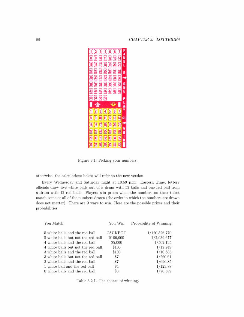
88 CHAPTER 3. LOTTERIES
Figure 3.1: Picking your numbers.
otherwise, the calculations below will refer to the new version.
Every Wednesday and Saturday night at 10:59 p.m. Eastern Time, lotteryofficials draw five white balls out of a drum with 53 balls and one red ball froma drum with 42 red balls. Players win prizes when the numbers on their ticketmatch some or all of the numbers drawn (the order in which the numbers are drawndoes not matter). There are 9 ways to win. Here are the possible prizes and theirprobabilities:
You Match You Win Probability of Winning
5 white balls and the red ball JACKPOT 1/120,526,7705 white balls but not the red ball $100,000 1/2,939,6774 white balls and the red ball $5,000 1/502,1954 white balls but not the red ball $100 1/12,2493 white balls and the red ball $100 1/10,6853 white balls but not the red ball $7 1/260.612 white balls and the red ball $7 1/696.851 white ball and the red ball $4 1/123.880 white balls and the red ball $3 1/70.389
Table 3.2.1. The chance of winning.

3.2. THE POWERBALL LOTTERY 89
If a player wins any prize except the jackpot and if she has not selected the PowerPlay option, she wins the amount of that prize. If she has selected the Power Playoption (which costs $1 dollar per ticket), then all prize amounts except the jackpotare multiplied by either 2, 3, 4, or 5. This multiplier is the same for all players ina given lottery, and is determined by the drawing of a Power Play ball at the timethe other balls are drawn. There are five Power Play balls; two of them have a 5on them, and the numbers 2, 3, and 4 each appear on one of the other three balls.
If the player wins the jackpot, she must share it equally with all other players (ifthere are any) who have also won the jackpot. A few other comments concerningthe jackpot are in order. First, the winning players have 60 days after they have wonto declare whether they want a lump sum payment or a series of 30 equal paymentsover the next 29 years (the first payment is made immediately and the others aremade at the end of each subsequent year). This latter type of award is called anannuity. Second, the lump sum is typically only about 60% of the announced valueof the jackpot. The present value of the annuity is equal to the lump sum amount.The announced value of the jackpot is the undiscounted total of all the annuitypayments. An example will help clear this up.
Suppose that the jackpot is announced to be $30 million. If there is only onewinner, and he chooses the annuity option, he will receive 30 equal payments of$1 million each. Thus, in some sense he has won $30 million. However, whenconsidering future payments, one usually discounts those future payments. Thepoint here is that having $100 today is in a sense equal to having $110 one yearfrom today, if one can earn 10% interest on cash. In a symmetric fashion, beingawarded a payment of $100 that will be paid one year from today is equal to having10/11 of $100 (or $90.91) today. The present value of the 30 equal payments of $1million is determined by discounting each of the last 29 payments by an amountdetermined by the date on which the payment will be made.
3.2.2 Calculating the Probabilities
The first question we ask is: how are these probabilities determined? In whatfollows, we will calculate various probabilities assuming the player has bought oneticket. This is a counting problem that requires that you understand one simplecounting rule: if you can do one task in n ways and, for each of these, another taskin m ways, the number of ways the two tasks can be done is mn. A simple treediagram makes this principle very clear.
When you watch the numbers being drawn on television, you see that, as thefive winning white balls come out of the drum, they are lined up in a row. The firstball could be any one of 53. For each of these possibilities the next ball could beany of 52, etc. Hence the number of possibilities for the way the five white ballscan come out in the order drawn is
53 · 52 · 51 · 50 · 49 = 344, 362, 200 .
But to win a prize, the order of these 5 white balls does not count. Thus, for aparticular set of 5 balls all possible orders are considered the same. Again by our

90 CHAPTER 3. LOTTERIES
counting principle, there are 5 ·4 ·3 ·2 ·1 = 120 possible orders. Thus, the number ofpossible sets of 5 white balls not counting order is 344, 262, 200/120 = 2, 869, 685.This is the familiar problem of choosing a set of 5 objects out of 53, and we denotethis by C(53, 5). Such numbers are called binomial coefficients. We can express ourresult as
C(53, 5) =(
535
)=
53!5!48!
= 2, 869, 685 .
Now for each pick of five white numbers there are 42 possibilities for the red Power-ball, so the total number of ways the winning six numbers can be chosen is
42 · C(53, 5) = 120, 526, 770 .
We will need this number often and denote it by b (for big).The lottery officials go to great pains to make sure that all b possibilities are
equally likely. So, a player has one chance in 120,526,770 of winning the jackpot.Of course, the player may have to share this prize.
We note that on the Powerball website, the column corresponding to the lastcolumn in Table 3.1 is labeled ’odds.’ The numbers in the column are in factprobabilities, not odds. Because the probabilities are small, there is not muchdifference between odds and probabilities. However, this is a good excuse to getthe difference between the two concepts straightened out. The media prefers to useodds, and textbooks prefer to use probability or chance. Here the chance of winningthe jackpot is 1 in 120,526,770, whereas the odds are 1 to 120,526,769 in favor (or120,526,769 to 1 against).
To win the $100,000 second prize, the player must get the 5 white numberscorrect but miss the Powerball number. How many ways can this be accomplished?There is only one way to get the set of five white numbers, but the player’s Powerballpick can be any of the 41 numbers different from the red number that was drawn.Thus, the chance of winning second prize is 41 in 120,526,770; rounded to thenearest integer this is 1 in 2,939,677.
One can find the probability of winning the second prize by pointing out theprobability that you get the 5 white numbers correct is 1/C(53,5). The chance ofnot getting the red ball correct is 41/42. Since these events are independent, thechance that they both happen is the product of their individual probabilities.
When there were 45 white balls and 45 red balls, the ticket listed the chances ofgetting only the red ball as 1 in 84. This often seemed wrong to players who havehad elementary probability, as the following exchange from the Powerball FAQ1
illustrates:
COULD YOUR ODDS BE WRONG?
I have a simple question. You list the odds of matching only the power-ball as one in 84 on the powerball ”ways to win” page. From my un-derstanding of statistics (I could be wrong, but I got an A), the oddsof selecting one number out of a group is simply one over the number
1From the Multi-State Lottery Association web site at http://www.musl.com/

3.2. THE POWERBALL LOTTERY 91
of choices. Since there are not 84 choices for the powerball, may I as-sume the balls are somehow ”fixed” so that some are more commonthan others? Otherwise, the listed odds are somehow defying the lawsof statistics. I am really very eager to hear your explanation, so pleasereturn my message. Thank you.
Susan G., via the Internet.
This is one of the most common questions we get about the statisticsof the game. If you could play only the red Powerball, then your oddsof matching it would indeed be 1 in 45. But to win the $1 prize formatching the red Powerball alone, you must do just that; match thered Powerball ALONE. When you bet a dollar and play the game, youmight match one white ball and the red Powerball. You might matchthree white balls and the red Powerball. To determine the probabilityof matching the red Powerball alone, you have to factor in the chancesof matching one or more of the white balls too.
C. S.
To win this last prize you must choose your six numbers so that only the Powerballnumber is correct. In the old version of the Powerball lottery this would be doneas follows: there are 45 · C(45, 5) = 54, 979, 155 ways to choose your six numbers.But here your first 5 numbers must come from the 40 numbers not drawn by thelottery. This can happen in C(40, 5) = 658, 008 ways. Now there is only one way tomatch the Powerball number, so overall you have 658,008 chances out of 54,979,155to win this prize. This reduces to 1 chance in 83.55, or about 1 chance in 84, inagreement with the official lottery pronouncement.
The same kind of reasoning of course carries over to the present version of thegame. To find the chance of winning any one of the prizes we need only count thenumber of ways to win the prize and divide this by the total number of possiblepicks b. Let n(i) be the number of ways to win the ith prize. Then the values ofn(i) are shown in Table 3.2 below.
Number of Ways Match
n(1) = 1 all six ballsn(2) = 41 5 white balls but not the red balln(3) = C(5, 4) · C(48, 1) 4 white balls and the red balln(4) = n(3) · 41 4 white balls but not the red balln(5) = C(5, 3) · C(48, 2) 3 white balls and the red balln(6) = n(5) · 41 3 white balls but not the red balln(7) = C(5, 2) · C(48, 3) 2 white balls and the red balln(8) = C(5, 1) · C(48, 4) 1 white ball and the red balln(9) = C(48, 5) only the red ball
Table 3.2.2. How many ways can you win a particular prize?

92 CHAPTER 3. LOTTERIES
Dividing these numbers by b, we obtain the chance of winning the correspondingprizes given in Table 3.2.1. Adding all the of n(i) values gives a total of 3,342,046ways to win something. Thus we get an overall chance of winning of 3, 342, 046/b =0.02773, which is about 1 in 36.
In a textbook, we would be apt to give the results of Table 3.1 as:
You Match You Win Probability of Winning
5 white balls and the red ball JACKPOT 0.00000000835 white balls but not the red ball $100,000 0.00000034024 white balls and the red ball $5,000 0.00000199134 white balls but not the red ball $100 0.00008164163 white balls and the red ball $100 0.00093589173 white balls but not the red ball $7 0.00383715582 white balls and the red ball $7 0.00143503391 white ball and the red ball $4 0.00807206560 white balls and the red ball $3 0.0142068355
Table 3.2.2. The probabilities of winning.
As noted earlier, rounding the reciprocals of these probabilities to the nearest integergives the numbers reported as ”odds” on the lottery ticket.
Discussion Question: Which of the two methods for presenting the chances of win-ning, Table 3.1 or Table 3.3, do you think is best understood by the general public?Which do you prefer?
3.2.3 What is your expected winning for a $1 ticket?
The value of a gambling game is usually expressed in terms of the player’s expectedwinning. If there are n prizes and p(i) is the probability of winning the ith prizew(i), then your expected winning is:
E = w(1) · p(1) + w(2) · p(2) + ... + w(n)· (n) .
We will first discuss the case when the Power Play option is not chosen. Later,we will summarize the corresponding case when this option is chosen. For all prizes,except the jackpot, we can assume we know the value of the prize. However, sincethe size of the jackpot differs significantly from drawing to drawing, we will want tofind the expected winning for different jackpot sizes. In the 508 drawings from thebeginning of the lottery on April 22, 1992 through March 1, 1997 the jackpot waswon 75 times. It was shared with one other winner 11 times. During this periodthe jackpot prize varied from $2 million to $314,900,000.
If x is the amount of the jackpot and p(i) the probability of winning the ithprize, the expected winning is:
E = x · p(1) + 100, 000 · p(2) + 5000 · p(3) + 100 · p(4) + 100 · p(5)
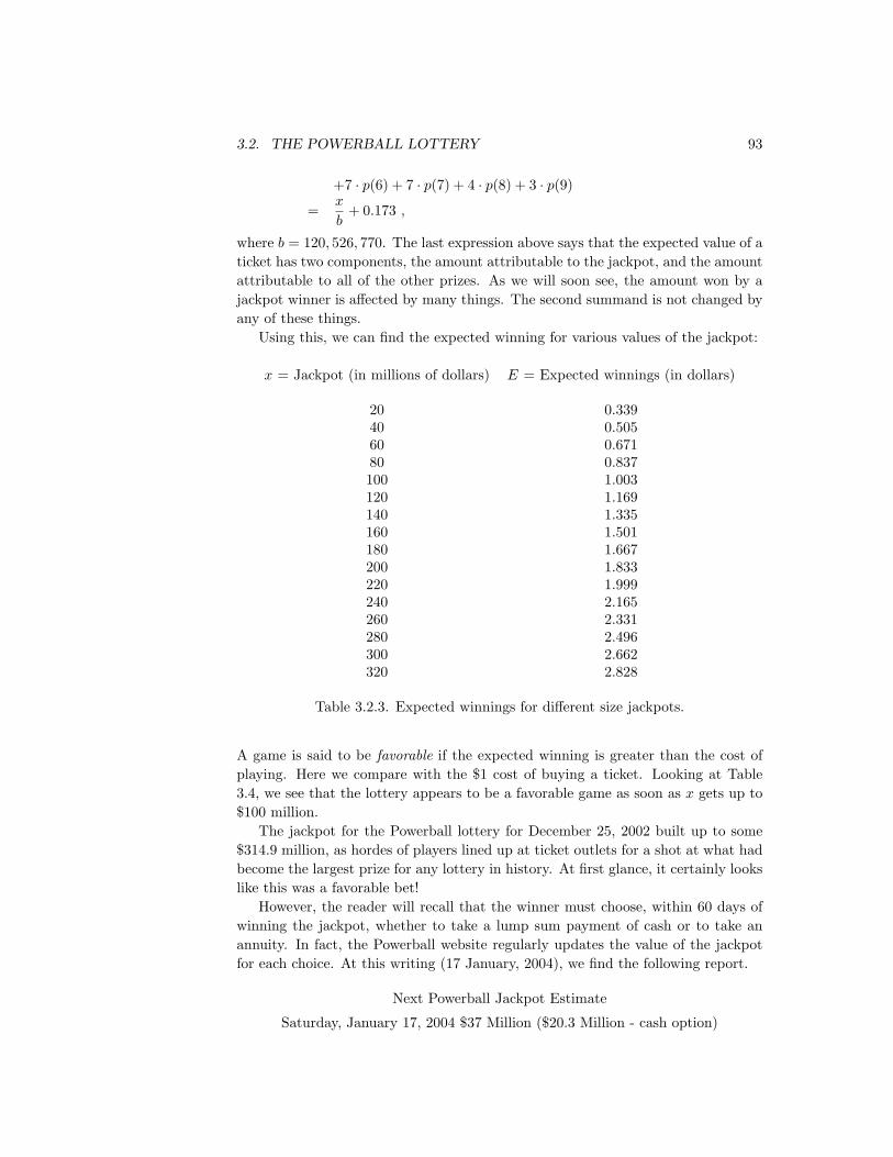
3.2. THE POWERBALL LOTTERY 93
+7 · p(6) + 7 · p(7) + 4 · p(8) + 3 · p(9)
=x
b+ 0.173 ,
where b = 120, 526, 770. The last expression above says that the expected value of aticket has two components, the amount attributable to the jackpot, and the amountattributable to all of the other prizes. As we will soon see, the amount won by ajackpot winner is affected by many things. The second summand is not changed byany of these things.
Using this, we can find the expected winning for various values of the jackpot:
x = Jackpot (in millions of dollars) E = Expected winnings (in dollars)
20 0.33940 0.50560 0.67180 0.837100 1.003120 1.169140 1.335160 1.501180 1.667200 1.833220 1.999240 2.165260 2.331280 2.496300 2.662320 2.828
Table 3.2.3. Expected winnings for different size jackpots.
A game is said to be favorable if the expected winning is greater than the cost ofplaying. Here we compare with the $1 cost of buying a ticket. Looking at Table3.4, we see that the lottery appears to be a favorable game as soon as x gets up to$100 million.
The jackpot for the Powerball lottery for December 25, 2002 built up to some$314.9 million, as hordes of players lined up at ticket outlets for a shot at what hadbecome the largest prize for any lottery in history. At first glance, it certainly lookslike this was a favorable bet!
However, the reader will recall that the winner must choose, within 60 days ofwinning the jackpot, whether to take a lump sum payment of cash or to take anannuity. In fact, the Powerball website regularly updates the value of the jackpotfor each choice. At this writing (17 January, 2004), we find the following report.
Next Powerball Jackpot Estimate
Saturday, January 17, 2004 $37 Million ($20.3 Million - cash option)

94 CHAPTER 3. LOTTERIES
Select the cash option and receive the full cash amount in the prizepool. Select the annuity option and we will invest the money and paythe annuity amount to you over 30 annual payments.
The $37 million here is analogous to the $314.9 million from December 25, 2002,and is the number that the media likes to hype. But note that this corresponds tothe annuity amount to be paid out over time, not the immediate cash value. Notonly are you not going to get this money tomorrow–the lottery doesn’t even haveit on hand! This is explained further in an earlier excerpt from the FAQ:
When we advertise a prize of $25 million paid over 29 years (30 pay-ments), we actually have about $13 million in cash. When someonewins the jackpot, we take bids to purchase government securities tofund the prize payout. We take the $13 million in cash and buy U.S.government-backed securities to fund these payments. We buy bondsthat will mature in one year at $1 million, then bonds which will ma-ture in two years at $1 million, etc. Generally, the longer the time tomaturity, the cheaper the bonds.
The cash option on the $314.9 million from December 25 was about $170 million.From Table 3.4, we see that this still looks like a favorable bet, with expected valueof about 2. We have been assuming that the player has elected the lump sum cashpayment, and treating the annuity as equivalent in present value terms. You maywant to think harder about this. An article in the Star Tribune by Julie Trip (June7, 1998, Metro section p. 1D) discusses the question of lump sum or annuity. Thearticle is based on an interview with Linda Crouse, a financial planner and certifiedpublic accountant in Portland, Oregon. (Note that this article was written in themiddle regime of the lottery.) From this article we read:
Crouse ran numbers to help determine whether it’s better to take awindfall in payments over time - an annuity - or in a lump sum.
Crouse used the Powerball jackpot as an example to determine whichpays off in the long run: the ticket that pays the winner $104.3 millionnow or pays $7.7 million annually for 25 years. (Both are before taxes.)
The annuity represents a 5.4 percent return. That sounds easy to beatif you take the lump sum and invest it - until you consider the hugenegative effect of paying all the taxes up front instead of over 25 years.Figure 45 percent of the payout - $46.9 million - goes to state and federaltaxes right off the bat. If you invest the remaining $57.4 million andreceive an average return of 8 percent, you still can’t beat the annuity.After all taxes are paid, you receive $4,235,000 annually for the annuityvs. $3,991,000 for the lump sum you invested at 8 percent.
Beyond about a 9 percent return, you start to beat the annuity.
Of course, one should consider the fact that the annuity is a guaranteed paymentwhile your investments are subject to the volatility of the way you invest yourmoney.

3.2. THE POWERBALL LOTTERY 95
Well, at least with the lump sum above, we convinced ourselves that we hada favorable game. Alas, there is another rub. We have been implicitly assumingthat if we hold the lucky numbers, we will get the whole prize! But if other ticketholders have selected the same numbers, the jackpot will be split. This will be aparticularly important factor when large number of tickets are sold. As the jackpotgrows, an increasing number of tickets are sold. For example, for the December 25,2002 Powerball lottery, it was estimated that 113 million tickets were sold.
The chance of having to share the jackpot depends upon several factors. First,it depends upon the number of tickets sold. Second, it depends upon whether thenumbers are all roughly equally likely to be chosen. In the Easy Pick method, thenumbers are chosen by the computer, and we can therefore assume that they areall equally likely. We are told that about 70% of tickets sold in a typical lottery arechosen by the Easy Pick method. Probably this percentage is even larger when thejackpot is large since people tend to buy a number of tickets and would be morelikely to use the Easy Pick method when they do this.
The remaining tickets have numbers that are chosen by the ticket buyers. Fig-ure 3.7 (displayed later in the chapter) shows that the numbers are not chosen withequal probabilities by the buyers. In a given winning set of numbers, some of themwill be more likely than others to have been chosen by these buyers. We expectthat this will have little effect on the number of jackpot winners. *****Simulatethis.
Because the effect of the non-Easy Pick tickets is small, we will usen = 113, 000, 000 as the number of tickets sold, and we will assume that theywere all chosen by the Easy Pick method. The probability that a particular ticketis the winning ticket is 1/120, 526, 770. The probability of k winners can be ob-tained from a binomial distribution with p = 1/120, 526, 770 and n = 113, 000, 000.The expected number of winning tickets is
np =113, 000, 000120, 526, 770
= 0.94 .
Since p is small and n is large we can use the Poisson approximation:
p(k) = e−m mk
k!,
where m = 0.94. Carrying out this calculation gives:
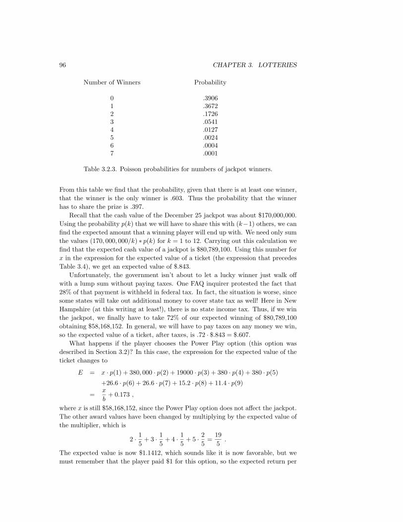
96 CHAPTER 3. LOTTERIES
Number of Winners Probability
0 .39061 .36722 .17263 .05414 .01275 .00246 .00047 .0001
Table 3.2.3. Poisson probabilities for numbers of jackpot winners.
From this table we find that the probability, given that there is at least one winner,that the winner is the only winner is .603. Thus the probability that the winnerhas to share the prize is .397.
Recall that the cash value of the December 25 jackpot was about $170,000,000.Using the probability p(k) that we will have to share this with (k−1) others, we canfind the expected amount that a winning player will end up with. We need only sumthe values (170, 000, 000/k) ∗ p(k) for k = 1 to 12. Carrying out this calculation wefind that the expected cash value of a jackpot is $80,789,100. Using this number forx in the expression for the expected value of a ticket (the expression that precedesTable 3.4), we get an expected value of $.843.
Unfortunately, the government isn’t about to let a lucky winner just walk offwith a lump sum without paying taxes. One FAQ inquirer protested the fact that28% of that payment is withheld in federal tax. In fact, the situation is worse, sincesome states will take out additional money to cover state tax as well! Here in NewHampshire (at this writing at least!), there is no state income tax. Thus, if we winthe jackpot, we finally have to take 72% of our expected winning of $80,789,100obtaining $58,168,152. In general, we will have to pay taxes on any money we win,so the expected value of a ticket, after taxes, is .72 · $.843 = $.607.
What happens if the player chooses the Power Play option (this option wasdescribed in Section 3.2)? In this case, the expression for the expected value of theticket changes to
E = x · p(1) + 380, 000 · p(2) + 19000 · p(3) + 380 · p(4) + 380 · p(5)
+26.6 · p(6) + 26.6 · p(7) + 15.2 · p(8) + 11.4 · p(9)
=x
b+ 0.173 ,
where x is still $58,168,152, since the Power Play option does not affect the jackpot.The other award values have been changed by multiplying by the expected value ofthe multiplier, which is
2 · 15
+ 3 · 15
+ 4 · 15
+ 5 · 25
=195
.
The expected value is now $1.1412, which sounds like it is now favorable, but wemust remember that the player paid $1 for this option, so the expected return per

3.2. THE POWERBALL LOTTERY 97
Figure 3.2: Powerball Sales vs. Jackpot Size.
dollar is $.057, which is slightly worse than it was before. par Perhaps we have nowexplained the famous quote:
”The lottery: A tax on people who flunked math.”
– Monique Lloyd
Discussion Question: Suppose that someone buys two lottery tickets, and fills themout with the same six numbers. How does this affect his expected value?
3.2.4 Is the expected value of a ticket every greater than $1?
We saw above that even in the record jackpot drawing of December 25, 2002, theexpected value of a ticket was significantly less than $1. We now consider whether,for certain jackpot sizes, the expected value of a ticket ever exceeds $1. To do this,we need to be able to estimate the number of tickets sold as a function of the jackpotsize. This has been done for the Powerball lottery, by Emily Oster, in her seniorthesis at Harvard.2 Figure 3.2 shows the data for the Powerball lottery from 1992to 2000.
Oster used a log-linear fit to arrive at the following equation. In this equation,si denotes the number of tickets sold in the i’th lottery, in millions, and pi denotesthe announced size of the i’th jackpot, in millions:
log(si) = 15.558 + .016pi ,
or equivalently,si = (5, 712, 000)(1.0161)pi .
2Emily Oster, Dreaming Big: Why Do People Play the Powerball?, Harvard University, March2002.
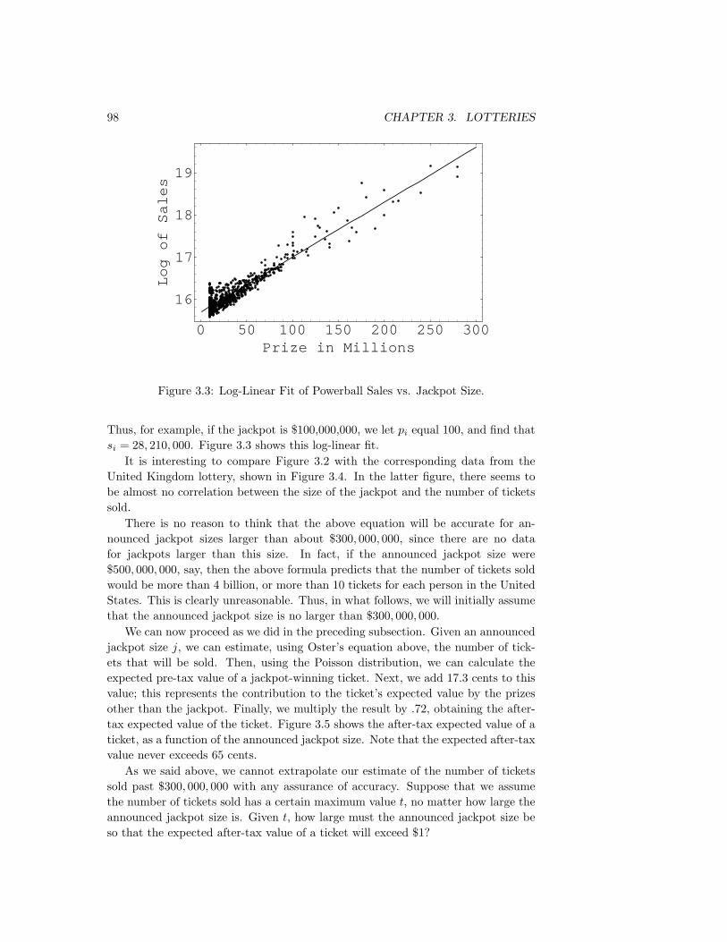
98 CHAPTER 3. LOTTERIES
0 50 100 150 200 250 300Prize in Millions
16
17
18
19Log
of
Sales
Figure 3.3: Log-Linear Fit of Powerball Sales vs. Jackpot Size.
Thus, for example, if the jackpot is $100,000,000, we let pi equal 100, and find thatsi = 28, 210, 000. Figure 3.3 shows this log-linear fit.
It is interesting to compare Figure 3.2 with the corresponding data from theUnited Kingdom lottery, shown in Figure 3.4. In the latter figure, there seems tobe almost no correlation between the size of the jackpot and the number of ticketssold.
There is no reason to think that the above equation will be accurate for an-nounced jackpot sizes larger than about $300, 000, 000, since there are no datafor jackpots larger than this size. In fact, if the announced jackpot size were$500, 000, 000, say, then the above formula predicts that the number of tickets soldwould be more than 4 billion, or more than 10 tickets for each person in the UnitedStates. This is clearly unreasonable. Thus, in what follows, we will initially assumethat the announced jackpot size is no larger than $300, 000, 000.
We can now proceed as we did in the preceding subsection. Given an announcedjackpot size j, we can estimate, using Oster’s equation above, the number of tick-ets that will be sold. Then, using the Poisson distribution, we can calculate theexpected pre-tax value of a jackpot-winning ticket. Next, we add 17.3 cents to thisvalue; this represents the contribution to the ticket’s expected value by the prizesother than the jackpot. Finally, we multiply the result by .72, obtaining the after-tax expected value of the ticket. Figure 3.5 shows the after-tax expected value of aticket, as a function of the announced jackpot size. Note that the expected after-taxvalue never exceeds 65 cents.
As we said above, we cannot extrapolate our estimate of the number of ticketssold past $300, 000, 000 with any assurance of accuracy. Suppose that we assumethe number of tickets sold has a certain maximum value t, no matter how large theannounced jackpot size is. Given t, how large must the announced jackpot size beso that the expected after-tax value of a ticket will exceed $1?

3.2. THE POWERBALL LOTTERY 99
0 2 4 6 8 10 12 14Jackpot Size Hin millionsL
0
20
40
60
80
100
120
SalesHin
millionsL
Figure 3.4: United Kingdom Sales vs. Jackpot Size.
0 50 100 150 200 250 300Prize in Millions
0.2
0.3
0.4
0.5
0.6
Expected
Value
Figure 3.5: Expected after-tax value of a ticket vs. announced jackpot size.
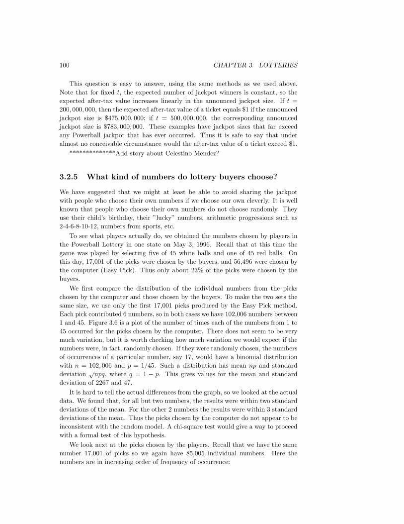
100 CHAPTER 3. LOTTERIES
This question is easy to answer, using the same methods as we used above.Note that for fixed t, the expected number of jackpot winners is constant, so theexpected after-tax value increases linearly in the announced jackpot size. If t =200, 000, 000, then the expected after-tax value of a ticket equals $1 if the announcedjackpot size is $475, 000, 000; if t = 500, 000, 000, the corresponding announcedjackpot size is $783, 000, 000. These examples have jackpot sizes that far exceedany Powerball jackpot that has ever occurred. Thus it is safe to say that underalmost no conceivable circumstance would the after-tax value of a ticket exceed $1.
**************Add story about Celestino Mendez?
3.2.5 What kind of numbers do lottery buyers choose?
We have suggested that we might at least be able to avoid sharing the jackpotwith people who choose their own numbers if we choose our own cleverly. It is wellknown that people who choose their own numbers do not choose randomly. Theyuse their child’s birthday, their ”lucky” numbers, arithmetic progressions such as2-4-6-8-10-12, numbers from sports, etc.
To see what players actually do, we obtained the numbers chosen by players inthe Powerball Lottery in one state on May 3, 1996. Recall that at this time thegame was played by selecting five of 45 white balls and one of 45 red balls. Onthis day, 17,001 of the picks were chosen by the buyers, and 56,496 were chosen bythe computer (Easy Pick). Thus only about 23% of the picks were chosen by thebuyers.
We first compare the distribution of the individual numbers from the pickschosen by the computer and those chosen by the buyers. To make the two sets thesame size, we use only the first 17,001 picks produced by the Easy Pick method.Each pick contributed 6 numbers, so in both cases we have 102,006 numbers between1 and 45. Figure 3.6 is a plot of the number of times each of the numbers from 1 to45 occurred for the picks chosen by the computer. There does not seem to be verymuch variation, but it is worth checking how much variation we would expect if thenumbers were, in fact, randomly chosen. If they were randomly chosen, the numbersof occurrences of a particular number, say 17, would have a binomial distributionwith n = 102, 006 and p = 1/45. Such a distribution has mean np and standarddeviation
√npq, where q = 1 − p. This gives values for the mean and standard
deviation of 2267 and 47.It is hard to tell the actual differences from the graph, so we looked at the actual
data. We found that, for all but two numbers, the results were within two standarddeviations of the mean. For the other 2 numbers the results were within 3 standarddeviations of the mean. Thus the picks chosen by the computer do not appear to beinconsistent with the random model. A chi-square test would give a way to proceedwith a formal test of this hypothesis.
We look next at the picks chosen by the players. Recall that we have the samenumber 17,001 of picks so we again have 85,005 individual numbers. Here thenumbers are in increasing order of frequency of occurrence:
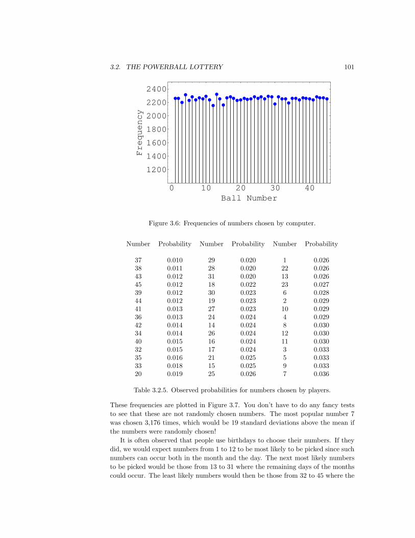
3.2. THE POWERBALL LOTTERY 101
0 10 20 30 40Ball Number
1200
1400
1600
1800
2000
2200
2400
Frequency
Figure 3.6: Frequencies of numbers chosen by computer.
Number Probability Number Probability Number Probability
37 0.010 29 0.020 1 0.02638 0.011 28 0.020 22 0.02643 0.012 31 0.020 13 0.02645 0.012 18 0.022 23 0.02739 0.012 30 0.023 6 0.02844 0.012 19 0.023 2 0.02941 0.013 27 0.023 10 0.02936 0.013 24 0.024 4 0.02942 0.014 14 0.024 8 0.03034 0.014 26 0.024 12 0.03040 0.015 16 0.024 11 0.03032 0.015 17 0.024 3 0.03335 0.016 21 0.025 5 0.03333 0.018 15 0.025 9 0.03320 0.019 25 0.026 7 0.036
Table 3.2.5. Observed probabilities for numbers chosen by players.
These frequencies are plotted in Figure 3.7. You don’t have to do any fancy teststo see that these are not randomly chosen numbers. The most popular number 7was chosen 3,176 times, which would be 19 standard deviations above the mean ifthe numbers were randomly chosen!
It is often observed that people use birthdays to choose their numbers. If theydid, we would expect numbers from 1 to 12 to be most likely to be picked since suchnumbers can occur both in the month and the day. The next most likely numbersto be picked would be those from 13 to 31 where the remaining days of the monthscould occur. The least likely numbers would then be those from 32 to 45 where the

102 CHAPTER 3. LOTTERIES
0 10 20 30 40Ball Number
500
1000
1500
2000
2500
3000
3500Frequency
Figure 3.7: Frequencies of numbers chosen by players.
year of the birthday could occur but only for those at least 52 years old. Note thatthis is indeed what appears to be happening.
Discussion Questions:
1. We have seen that the numbers picked by the players fall into three sets, withthe property that numbers in the same set are approximately equally likely to bechosen, but numbers in different sets are not equally likely to be chosen. Let usdenote the three sets by
S1 = 1, 2, . . . , 12 ,
S2 = 13, 14, . . . , 31 ,
S3 = 32, 33, . . . , 45 .
The collection of all sets of five unequal numbers, between 1 and 45, written inincreasing order, serves as the sample space of all possible choices by the players.The numbers in S1, S2, and S3 occur with average frequencies .0306, .0234, and.0134, respectively. Using these frequencies, show that if a chosen set of numbershas all of its numbers in S1, then it occurs with probability 2.7× 10⁻⁸, while if allof its numbers are in S3, then it occurs with probability 4.3× 10⁻¹⁰. How does thisaffect the expected value of these two tickets, i.e. is there a difference between theexpected values of tickets of the above two types?
2. Using the above data from the December 25, 2002 lottery, we saw that theexpected value of one lottery ticket, after taxes, is $.607. Suppose someone buystwo tickets and puts the same numbers on both tickets. What is the expected valueof each ticket?
Finally, we look at the winning numbers to see if they could be considered tobe randomly chosen. Recall that the lottery officials try to ensure that they are.

3.2. THE POWERBALL LOTTERY 103
0 10 20 30 40Ball Number
0
20
40
60
80
Frequency
Figure 3.8: Winning number frequencies.
Here we have many fewer numbers so we expect more variation even if randomlychosen. Since there were 508 drawings in the period we are considering, we have6 · 508 = 3048 numbers. Now, if the numbers are randomly chosen, the number oftimes a particular numbers occurs has a binomial distribution with n = 3048 andp = 1/45. Such a distribution has a mean of 67.7 and standard deviation 8.14.The biggest deviations from the mean are about 2 standard deviations so this looksconsistent with the hypothesis that the numbers were randomly chosen. Again, wecould check this with a chi-square test.
3.2.6 Finding patterns
Recall that players choose their first five numbers to match the white balls separatelyfrom their choice of the Powerball number to match the red ball. Thus, if we arelooking for patterns in the way people choose their numbers, it is best to considerthe first five numbers by themselves. We recall that our data set consists of two setsof picks of size 17,001; the first set contains picks chosen by the Easy Pick method,and the second set contains picks chosen by the players. For the Easy Picks, wefound that 136 of these were represented twice and 2 were represented 3 times.
To see if we should have expected to find 3 picks the same, we use the solutionof the birthday problem, which is a well-known problem in probability. The mostbasic form of this problem asks for the probability that at least two people amonga set of k people will share a birthday. Part of the reason that this problem isinteresting stems from the fact that if one asks how many people are needed in aroom in order to have a fair bet that at least two of these people have the samebirthday, then the surprising answer is that only 23 people are needed.
In our case, we are asking a more difficult question: Given 17,001 choices froma set of size C(45, 5) = 1, 221, 759 (this is the number of possible choices of five

104 CHAPTER 3. LOTTERIES
numbers from 45 numbers), what is the probability that at least three of the choicesare equal? So, instead of 366 possible birthdays, there are now 1,221,759 possiblebirthdays. It can be calculated that in this case, the probability of finding three ormore choices the same is about .42. To see how this calculation can be done, see3.One can also calculate that there is only a probability of .002 of finding 4 or morethe same birthday. Thus we should not be surprised at finding 3 picks the same andshould not expect to find 4 the same. Again, the computer picks seem to conformto random choices.
We look next at the 17,001 picks of 5 numbers chosen by the lottery players.We found 966 sets of numbers that were represented more than once (compared to138 for the Easy Pick numbers). The largest number of times a particular set ofnumbers was chosen was 24. This occurred for the pick 02-14-18-21-39. Lookingat the order in which the picks were given to us, we noticed that these occurredconsecutively in blocks of 5, with the blocks themselves close together. The ticketon which you mark your numbers allows room for 5 sets of numbers. We concludedthat one player had made 24 picks all with the same five numbers. He at leastchose different Powerball numbers. The same explanation applied to the next mostpopular pick 08-12-24-25-27, which occurred 16 times.
The third most popular set 03-13-23-33-43 was picked by 13 people and wasmore typical of the patterns that people chose. In this version of Powerball, thenumbers were arranged on the ticket as shown below:
Pick 5 EP
01 02 03 04 05 06 07 08 0910 11 12 13 14 15 16 17 1819 20 21 22 23 24 25 26 2728 29 30 31 32 33 34 35 3637 38 39 40 41 42 43 44 45
Note that the pick 03-13-23-33-43 is an arithmetic sequence obtained by going downa diagonal starting with 03. Similarly, the set of numbers 01-11-21-31-41, which waschosen 10 times, corresponds to going down a diagonal starting with 01 and the set06-15-24-33-42, chosen 9 times, corresponds to going down a column starting with06. The most interesting pattern noticed was 01-09-23-37-45, occurring 8 times,which results from choosing the corner points and the middle point. Since we donot expect repetitions of 4 or more to occur by chance, we looked at all those thatoccurred 4 or more times. We could explain all but three such sets of 5 numbers.These were:
01-03-09-30-34 (occurred 5 times, always with Powerball number 40)05-06-16-18-23 (occurred 4 times, always with Powerball number 31)02-05-20-26-43 (occurred 4 times with different Powerball numbers) .
Here are two letters that appeared in The Times (London) related to the problemof people choosing popular numbers. The letters followed an article in The Times
3MathWorld, ”Birthday Problem,” http://mathworld.wolfram.com/BirthdayProblem.html

3.2. THE POWERBALL LOTTERY 105
stating that the inaugural drawing of the new British Lottery had five times thenumber of winners expected, including seven people who had to share the jackpot.They blamed this on the fact that the six winning numbers 03-05-14-22-30-44 hadfive numbers under 31 and most people chose low numbers. In this lottery, youchoose 6 numbers between 1 and 49 and have to get them all correct to win thejackpot. If you get three numbers correct you win £10. The amount you win forany other prize depends on the number of other people who win this prize.
The Times, 24 November 1994, letters to the editor.
Slim pickings in National Lottery
From Mr. George Coggan
Sir, With random choices, the odds against there being seven or morejackpot winners in the National Lottery when only 44 million ticketshave been sold are 23-1. This suggests that those who predicted thatlow numbers would be popular were right as the slightly disproportionatenumber of single digits (3 and 5 came up) would combine to producemore winners than would be produced by entirely random selections.
Mildly interesting, one might think, but then one suddenly realizes thatthere is a lurking danger that the rules create the possibility that when(as will happen sooner or later) three single digit numbers come upthe prize fund may not be enough to cover the Pounds 10 guaranteedminimum prize, never mind a jackpot. I estimate that if the number 7had come up instead of say 44 the prize fund in this first lottery wouldhave been about Pounds 5 million short of the guarantee. What thenpanic?
Yours sincerely,
GEORGE COGGAN,
14 Cavendish Crescent North,
The Park, Nottingham.
November 21. 1994 Tuesday
The Times, 29 November 1994, letter to the editor.
No need to fear a lottery shortfall
From the Director General of the National Lottery
Sir, Mr. George Coggan (letter, November 24) raises concerns about theNational Lottery Prize Fund’s ability to pay winners when ”popular”numbers are selected in the weekly draw.
We are aware that players do not choose numbers randomly but usebirthdays, sequences or other lucky numbers. This causes the number

106 CHAPTER 3. LOTTERIES
of winners to deviate each week from the number predicted by statis-tical theory. Experience from other lotteries shows that the numberof winners of the lower prizes can vary by up to 30 per cent from thetheoretical expectation.
In the first National Lottery game there were many more Pounds 10prize-winners than theory predicted. It is just as likely that future drawswill produce fewer than expected winners and, because each higher prizepool is shared between the winners, prize values will rise accordingly.
Mr. Coggan suggests a pessimistic scenario in which the cost of payingthe fixed Pounds 10 prizes to those who choose three correct numbersexceeds the prize fund. Best advice, and observations from other lotter-ies around the world, is that, even after allowing for the concentration on”popular” numbers, the chances of this happening are extremely remote.
Your readers will be reassured to know, however, that I have not reliedtotally upon statistics or evidence from other lotteries. Camelot’s licenseto operate the National Lottery also requires them to provide substantialadditional funds by way of deposit in trust and by guarantee to protectthe interests of the prize-winners in unexpected circumstances.
Yours faithfully,
PETER A. DAVIS
Director General, National Lottery
PO Box 4465
London SW1Y 5XL
November 25.
Of course, it is interesting to look at this problem for the Powerball lottery. Wenoted that, in our sample of 17,001 numbers where players picked their own num-bers, there were particular sets of five numbers for the white balls that were chosenas many as 10 times. For example the set of numbers 01-11-21-31-41 obtained bygoing down a diagonal starting at 1 in the box where you mark your numbers waschosen 10 times in our sample of 17,001.
The July 29, 1998 lottery set a new record for the jackpot size (this record wasbroken on December 25, 2002, as noted earlier). For the July 29, 1998 drawingthere were 210,800,000 tickets sold. If we assume that about 30% of the playerspick their own numbers, then using the above example, it is possible that the thereexists a set of white numbers that was picked by
.3(210800000)1700
= 37200
players. It will be recalled that a player who picks all five white numbers gets$100,000, so if the lottery officials had the bad luck to also choose this set of five

3.2. THE POWERBALL LOTTERY 107
5 10 15Waiting Time Hin weeksL
2
4
6
8
10
12
14
16
Frequency
Figure 3.9: Waiting times between jackpots.
numbers this would cost them 3.72 billion dollars! The new boxes are not as sym-metric as the old ones to which our data applied. This may help them with thispotential problem. It is also the case that the lottery computer is very unlikely tochoose a popular set of numbers. However, the lottery is protected in still anotherway. In the fine print that describes the lottery, it is stated that if there are toomany awards won, the officials reserve the right to divide a certain amount of moneyamong the prize winners, just like what is done with the jackpot. This last eventhas never happened in the history of the Powerball lottery.
3.2.7 How often is the jackpot won?
The size of the jackpot changes from one drawing to the next. If, on a given drawing,no one chooses the winning numbers, the jackpot is increased several million dollarsfor the next drawing. When there is a winner, the jackpot goes back to the minimumamount, which currently is 10 million dollars. The size of the increase when thereis no winner depends upon the number of tickets sold for the previous drawing. Weinvestigate the size of the jackpots through the years of the original rules.
We find, on the Powerball homepage, the amounts of the jackpot in all thedrawings under the original rules. The jackpots, from the beginning of the Powerballlottery on April 22, 1992 until March 1, 1997, range from 2 million to 111,240,463.The jackpot was won in 75 of these 805 drawings. 11 of these times there weretwo winners and never more than two winners. The total of all these jackpots was$2,206,159,204 with an average of $29,415,456. The average number of drawingsbetween jackpots being won was 6.72 or, since there are two drawing a week, about3 weeks. The distribution of times between jackpots is shown in Figure 3.9.
*****************Add the data for the waiting times between 1997 and thepresent.

108 CHAPTER 3. LOTTERIES
DISCUSSION QUESTION: The mode 6 seems rather over-represented. Can youthink of any explanation for this, or is it just chance?
It is interesting to ask what kind of a probability model would be appropriateto describe the time between winning the jackpot. The probability of the jackpotbeing won depends upon the number of tickets sold. (Actually, it depends uponthe number of different picks chosen.) If the same number of tickets were sold oneach drawing then the appropriate model would be: toss a coin with probability p
for heads until the first time heads turns up where 1/p is the average time betweenheads. Unfortunately, it is not at all reasonable to assume the same number oftickets will be sold. Here is what the Powerball FAQ says about this.
For a $10 million jackpot draw we sell about $11 million. For a $20million jackpot we sell about $13 million. With a $100 million jackpotwe sell $50 to $70 million for the draw (depending on time of year andother factors).
Let’s assume that, for a particular jackpot, n tickets are sold. Then the probabilitythat a particular person does not win the jackpot is (a − 1)/a, where, for the oldversion of the game,
a = 45 · C(45, 5) = 54, 979, 155 .
The probability that none of the tickets sold wins the jackpot is(a− 1
a
)n
.
Here is a table of these probabilities for some different values of the number oftickets sold.
Millions of Probabilitytickets sold no one wins
10 .83420 .69530 .57940 .48350 .40360 .33670 .280
Table 3.2.7. Probability no one wins the jackpot.
3.2.8 Other lotteries pose new questions
There are many other interesting questions that can be explored about lotteries.The questions that one asks depend, to some extent, on the nature of the lottery.For example, in September 1996 the Multi-State lottery introduced a new lotterycalled Daily Millions where the amount of the jackpot is always $1 million and, if

3.2. THE POWERBALL LOTTERY 109
you win, you don’t have to share it with another person who also has the samewinning pick (actually, if there are more than 10 such winners they share a $10million prize.) An article appeared in the Star Tribune shortly after this lotterywas introduced4. The article began as follows:
The lottery wizards said it wasn’t supposed to work this way.
Nearly five months after the Daily Millions lottery began, none of the34 million tickets sold has won the $1 million jackpot. The probabilityof such a long losing streak is 1 in 38.
The drought has lasted so long, “We even have solid believers in statis-tics questioning the wisdom of numbers,” quipped Charles Strutt, exec-utive director of the Multi-State Lottery Association, which runs DailyMillions and Powerball.
They’re not the only ones.
At the East Grand Forks, Minn., Holiday store, “People are startingto get a little disgusted with it,” said cashier Steve Nelson. The storehas been among the top sellers of Powerball tickets, but sales of DailyMillions tickets have declined.
The article states that the ticket sales in the first week of the lottery were $2.75million, but five months later, they had declined to $1.23 million.
The day after the above article appeared, the Daily Millions lottery had its firstwinner.
3.2.9 Using lottery stories to discuss coincidences
James Hanley5 has discussed how stories about lottery winners provide good exam-ples to discuss the meaning of apparent coincidences. Here is his first example6.
Lottery officials say that there is 1 chance in 100 million that the samefour-digit lottery numbers would be drawn in Massachusetts and NewHampshire on the same night. That’s just what happened Tuesday.
The number 8092 came up, paying $5,482 in Massachusetts and $4,500 inNew Hampshire. ”There is a 1-in-10,000 chance of any four digit numberbeing drawn at any given time,” Massachusetts Lottery Commissionofficial David Ellis said. ”But the odds of it happening with two statesat any one time are just fantastic,” he said.
What is the probability that the same four-digit lottery number would be drawnin Massachusetts and New Hampshire on the same night? What is the probability
4Doyle, Pat, “Daily Millions Beats Odds: No One Wins – 5-Month Losing Streak Puzzles EvenStatisticians,” Star Tribune, Minneapolis, 7 Feb. 1997, pg. 1B.
5Hanley, James A. ”Jumping to Coincidences, ” The American Statistician, Vol 46, No. 3, pp197-201.
6“Same Number 2-State Winner,” Montreal Gazette, September 10, 1981.

110 CHAPTER 3. LOTTERIES
that some two such lotteries have the same two numbers during a given periodof time? Is this different from a reporter noticing that the number that turnedup in the lottery in New Hampshire on Wednesday happened also to occur in theMassachusetts lottery on Saturday?
Here is another of Hanley’s examples7.
Defying odds in the realm of the preposterous–1 in 17 million–a womenwho won $3.9 million in the New Jersey state lottery last October hashit the jackpot again and yesterday laid claim to an addition $1.5 millionprize...
She was the first two time million-dollar winner in the history of NewJersey’s lottery, state officials said. They added that they had neverbefore heard of a person winning two million-dollar prizes in any of thenation’s 22 state lotteries.
For aficionados of miraculous odds, the numbers were mind boggling: Inwinning her first prize last Oct. 24, Mrs. Adams was up against odds of1 in 3.2 million. The odds of winning last Monday, when numbers weredrawn in a somewhat modified game, were 1 in 5.2 million.
And after due consultation with a professor of statistics at Rutgers Uni-versity, lottery officials concluded that the odds of winning the toplottery prize twice in a lifetime were 1 in about 17.3 trillion–that is,17,300,000,000,000.
Does it matter that she played the lottery many times, often buying more than oneticket? Again, are we talking about this happening somewhere, sometime? Shouldwe ever believe that something with these odds has happened?
3.2.10 Lottery systems
Richard Paulson8 observes that claims made about systems for improving yourchances at lotteries illustrate important statistical concepts. For example, peopleclaim that, by analyzing the historical data of winning numbers, it is possible topredict future winners. Indeed, lottery sites encourage this by making this historicaldata available. Sometimes the argument is simply that, when a particular numberhas not turned up as often as would be expected, then this number is more likelyto come up in the future. This is often called the ”gambler’s fallacy” and all toomany people believe it. The fact that it is not true is the basis for many beautifulapplications of chance processes called martingales.
Paulson remarks that he particularly enjoys discussing the following system.Consider, the six winning numbers in the Powerball Lottery. If they occur randomlytheir sum should be approximately normally distributed with mean 6(1+45)/2 =
7“Odds-Defying Jersey Woman Hits Lottery Jackpot 2nd Time,” New York Times, February14, 1986.
8Paulson, Richard A. ”Using Lottery Games to Illustrate Statistical Concepts and Abuses”,The American Statistician , Vol. 45, No. 3, pp. 202-204.

3.2. THE POWERBALL LOTTERY 111
138 and standard deviation approximately 32. Thus, sets of six numbers whose sumis more than 64 away from the mean 138, are not likely to occur as winning setsand should be avoided. It is better to pick six numbers whose sum is near 138. Weleave the reader to ponder this last system.
One of our teachers, the well-known probabilist Joseph Doob, was often askedfor a system to use when playing roulette. His advice ran as follows. Play red once.Then wait until there have been two blacks and play red again. Then wait untilthere have been three blacks and play red again. Continue in this manner. You willenjoy playing and not lose too much.

112 CHAPTER 3. LOTTERIES

Chapter 4
Scaling in Human Endeavor
4.1 Zipf’s Law
In 1916, the Frence stenographer J. B. Estoup1 noted that if one listed words in atext according to the frequency of their occurrence, the product of frequency (F )and rank (R) of the words is approximately constant. Pereto2 observed the samephenomena relating to corporate wealth. In his book3, George Zipf showed that thisconstant product law applied to the ranking of populations of cities and to manyother data sets. This became known as Zipf’s law.
One can check this law on large sets of text, using computers. The BritishNational Corpus (BNC) is a 100-million word collection of samples of written andspoken language from a wide range of sources, designed to represent a wide cross-section of current British English, both spoken and written. If the product of rankand frequency is a constant, then a log-log plot of frequency versus rank should bea straight line with slope -1. (To see why this should be so, assume that
F =c
R,
where c is a constant. Then
log F = log c− log R ,
which is a straight line with slope -1.)The log-log plot of the data is shown in Figure ??. The line with slope -1 fits the
higher part of the graph corresponding to the most common words. But to fit thelower part of the graph, corresponding to words used infrequently, we had to choosea line with larger negative slope -1.64. The need for different lines forthe frequentand the infrequent words was suggested by Ferrer-i-Cancho and Sole in their paper
1J. B. Estoup, Gammes Stenographiques, Intstitut Stenographicque de France, Paris, 1916.2Cours d’economie politique, Drox, Geneva, Switzerland, 1896 and Rouge, Lausanne et Paris,
18973G. K. Zipf, Human Behavior and the Principle of Least Effort: An Introduction to Human
Ecology, Addison-Wesley, 1949
113

114 CHAPTER 4. SCALING IN HUMAN ENDEAVOR
”Two regimes in the frequency of words and the origins of complex lexicons: Zipf’slaw revisited.”4
An interesting application of Zipf’s law was carried out by Gabriel Landini. TheVoynich manuscript is a famous manuscript shrouded in mystery. this mystery isdescribed by Victory Segal in her brief account of a BBC4 documentary in theSunday Times.5 She writes:
While it is easy to mock conspiracy theorists as loners in X Files T-shirts, this documentary explores a puzzle whose appeal stretches waybeyond the glow of the internet chat room. The Voynich manuscriptwas discovered in an Italian villa by an antiquaian book dealer, WilfredVoynich, early last century. Decorated with pictures of plants, stars, and“naked nymphs,” its 238 pages are written in an unreadable language,a peculiar grid of symbols that have resisted all attempts at translation.
Some think it is a code, others a language in its own right. It mightcome from the 13th century or it might be a modern forgery, perpetratedby Voynich himself. This is a perfect introduction to the manuscript andits lore, veering between theories at a dizzying rate. Roger Bacon, JohnDee, and Emperor Rudolph II all play their part, as do National SecurityCouncil cryptographers, Yale maths professors and an array of eccentricamateurs, from computer games programmers to herbalists. And, ofcourse, there is a man in South Carolina who thinks extraterrestrialshold the key.
One can find more details of the history and current research on the web. Weenjoyed the discussion here which has several nice pictures from the manuscriptincluding the one in Figure ??.
Several electronic versions of the Voynich manuscript which use arbitrary al-phabets to transcribe the symbols are available. These have been used to studystatistical properties of the manuscript. In particular, Landini used two of theseto see if Zipf’s law applied to the frequencies of the Voynich text. His results aredescribed here. Figurereffig shows a plot that he gives for the rank-frequency rela-tion using a translation called voynich.now. For comparison, Landini gives similarplots (shown in Figure ??) for several well-known text sources including Alice inWonderland.
Of course, it would be nice if one could conclude that the Voynich manuscriptis not a hoax from the fact that the frequencies of words in the Voynich manuscriptsatisfy Zipf’s law. However, it may not be correct to conclude this, since it hasbeen verified by a number of studies that words generated randomly also appear tosatisfy Zipf’s law. ********Put in description of power laws and Polya models.
Zipf did not give a mathematical formulation but, as the title of his book sug-gests, he had the idea that it was related to a principle of least effort. For the caseof development of a language Zipf wrote:
4Ferrer-i-Cancho, R. and Sole, R. V., Journal of Quantitative Linguistics, 8 (3), pgs. 165-173.5Segal, Victory, London Times, 8 Dec. 2002
4.2. LOTKA DISTRIBUTIONS 115
Whenever a person uses words to convey meanings he will automat-ically try to get his ideas across most efficiently by seeking a balancebetween the economy of a small wieldy vocabulary of more general ref-erence on the one hand, and the economy of a larger one of more precisereference on the other hand, with the result that the vocabulary of dif-ferent words in his resulting flow of speech will represent a vocabularybalance between our theoretical Forces of Unification and Diversifica-tion.
4.2 Lotka Distributions
4.3 Appendix
In this section, we show how to find the limiting distribution of one of the Polyamodels. We begin with a description of the model.
Description of Model: Start with one bin with one ball at time t = 1. We denotethis first ball as b1, and set b1 = 1. At every integer step t, starting with t = 2,add one ball bt. The value of bt will be the number of the bin into which the ball isplaced. With probability p, the ball bt goes into a new bin, so in this case,
bt = 1 + maxj<t
bj .
With probability (1− p), we pick a ball bj uniformly over j < t, and add bt to thebin that contains bj ; in other words, in this case we set bt = bj .
For each i ≥ 1, define fi,t to be the random variable whose value is the fractionof bins at time t that contain exactly i balls. We want to show that for each i ≥ 1,
limt→∞
fi,t
exists with probability 1.Define ni,t to be the random variable whose value is the number of bins at time
t with exactly i balls, and define nt to be the random variable representing thenumber of bins at time t with at least one ball. Clearly,
fi,t =ni,t
nt.
Consider first the case i = 1. At time t + 1, with probability p we add bt+1 toa new bin, which means that n1,t+1 = n1,t + 1. Otherwise, there are n1,t balls inbins with one ball, and t balls already placed, so with probability (1 − p)(n1,t/t),we put bt+1 in a bin that contains one ball; in this case, n1,t+1 = n1,t− 1. The finalpossibility is that we put bt+1 in a bin that contains more than one ball; in thiscase, n1,t+1 = n1,t. Thus, we have
E(n1,t+1) = E
(p(n1,t + 1) + (1− p)
(n1,t
t(n1,t − 1) +
(1− n1,t
t
)n1,t
))

116 CHAPTER 4. SCALING IN HUMAN ENDEAVOR
= E
(n1,t + p− (1− p)
n1,t
t
).
Using standard generating function techniques, one can show that for t ≥ 1,
E(n1,t) =p
2− pt +
2t
p− 2(−1)t 1− p
t
=p
2− pt + o(t) .
Since nt is counting the number of new bins up to and including time t, togetherwith the original bin, we see that
E(nt) = 1 + p(t− 1) ∼ pt .
Of course, one cannot conclude from these statements about expected value that
E(f1,t) ∼1
2− p,
although one could conjecture that this is true. In order to prove that such astatement is true, it suffices to show that both of the sets of random variables ni,tand nt are usually very close to their mean. This would show that with highprobability, the ratio ni,t/nt is near the ratio of the means. The sequence nt isessentially a sequence of binomially distributed random variables, so it is easy todeal with. The sequence ni,t is a little more difficult. We will consider how to dothis once we have determined what the limit of fi,t should be.
If i ≥ 2, we have
E(ni,t+1) = E
(pni,t + (1− p)
(ini,t
t(ni,t − 1) +
(i− 1)ni−1,t
t(ni,t + 1) +
(1− (i− 1)ni−1,t + ini,t
t
)ni,t
))
=(
1− i(1− p)t
)E(ni,t) +
(i− 1)(1− p)t
E(ni−1,t) .
Suppose that we have shown that
E(ni−1,t) ∼ Ki−1t
for some constant Ki−1. (We have shown that K1 = p/(2−p).) If there is a constantKi such that
E(ni,t) ∼ Kit ,
what would the value of Ki be? One can show that
Ki ∼ i(1− p)(Ki−1 −Ki)− (1− p)Ki−1 ,

4.3. APPENDIX 117
which implies that for i ≥ 2,
Ki =(i− 1)(1− p)1 + i(1− p)
Ki−1 .
Since we don’t know that Ki exists for i ≥ 2, let us define K∗i by the equations
K∗1 =
12− p
and for i ≥ 2,
K∗i =
(i− 1)(1− p)1 + i(1− p)
K∗i−1 .
(We would like to show that Ki exists and equals K∗i .) If any of this is right, then
it must be true that∞∑
i=1
K∗i = p ,
since the left-hand side, multiplied by t, is asymptotically the number of bins filledwith balls at time t, which we know is close to pt with high probability.
Here are the first few values of K∗i :
K∗1 =
(p
2− p
)K∗
2 =(
1− p
3− 2p
)(p
2− p
)K∗
3 =(
2− 2p
4− 3p
)(1− p
3− 2p
)(p
2− p
).
The sum of this series can be calculated using hypergeometric functions. Specifi-cally, the hypergeometric function F (α, β, γ; z) is defined as follows:
F (α, β, γ; z) = 1 +αβ
γ1!z +
(α)(α + 1)(β)(β + 1)(γ)(γ + 1)2!
z2 +
(α)(α + 1)(α + 2)(β)(β + 1)(β + 2)(γ)(γ + 1)(γ + 2)3!
z3 + . . . .
It can be shown that
F (α, β, γ; z) =1
B(β, γ − β)
∫ 1
0
tβ−1(1− t)γ−β−1(1− tz)−α dt ,
if Re(γ) > Re(β) > 0. In the above equation, B(x, y) is the beta function, and isdefined by
B(x, y) =∫ 1
0
tx−1(1− t)y−1 dt .
It is relatively straightforward to show that∞∑
i=1
K∗i =
p
2− pF (1, 1, 2 + 1/(1− p); 1) ,

118 CHAPTER 4. SCALING IN HUMAN ENDEAVOR
and it is easy to calculate that the right-hand side of the above equation equals p.We can now proceed to the general case. Let
ai,t = E(ni,t) ,
and letbi,t =
ai,t
t.
Definegi(x) = bi,1x + bi,2x
2 + . . . .
We have already shown that
g1(x) =p
2− p(1− x)−1 + 1− 2
2− p(1− x)1−p .
(This is the equation that leads to our expression for E(n1,t).) In general, it is thecase that
gi(x) = Ai(1− x)−1 + Bi +i∑
j=1
Ci,j(1− x)j(1−p) ,
where the coefficients on the right-hand side are defined by
Ai =(i− 1)(1− p)
1 + i− ipAi−1 ,
if i > 1, and A1 = p/(2− p);
Bi =i− 1
iBi−1 ,
if i > 1, and B1 = 1;
Ci,j = (i− 1)Ci−1,j
i− j,
if i > 1 and j < i;
Ci,i = − (i− 1)(1− p)(1 + i− ip)
Ai−1 −(i− 1)(1− p)
(i− ip)Bi−1 − (i− 1)
i−1∑j=1
Ci−1,j
i− j,
if i > 1, and C1,1 = −2/(2− p).Where does this leave us? The above can be used to show that for all i ≥ 1,
E(ni,t) ∼ Ait = K∗i t ,
which is what we conjectured is true.Now, following Bollobas et al., we fix i ≥ 1 and n ≥ 1, and define a sequence of
random variables Xtnt=1 as follows:
Xt = E(ni,n|b1, b2, . . . , bt−1) .
This sequence is a martingale. We want to show that there is a c such that
|Xt+1 −Xt| ≤ c

4.3. APPENDIX 119
for 1 ≤ t < n. The reason that this is useful is the following theorem, due toAzuma6 and Hoeffding7.
Theorem 4.1 (Azuma-Hoeffding inequality) Let Xtnt=1 be a martingale with
|Xt+1 −Xt| ≤ c for t = 1, . . . , n. Then
P(|Xn −X1| ≥ x
)≤ exp
(− x2
2c2n
).
2
Here is an argument (modeled on the one in Bollobas et al.8) that shows that c canbe taken to be 2 in our model. At time t + 1, we choose, with probability p, a newbin numbered nt +1 (in other words, we set bt+1 equal to nt +1) or else we choose,with probability (1− p)/t, a j with 1 ≤ j ≤ t, and set bt+1 = bj .
Now consider two possible choices that were made at time t + 1 in the mannerdescribed above. We want to understand how much these two choices can affectthe number ni,n. So, for example, let’s assume that one choice was a new bin b∗,and the other choice was a bj , with j ≤ t. Any subsequent choice in either caseinvolving bins other than b∗ or bj will proceed with the same probability in eithercase. Thus, the only two bins which might have a different number of balls in thetwo cases are bins b∗ and bj . This means that in the two cases, the values of ni,n
differ by at most 2.We can now apply the Azuma-Hoeffding inequality to the sequence ni,t. We
see that X1 = E(ni,n) and Xn = ni,n, so the inequality implies that
P(|ni,n − E(ni,n)| ≥ x
)≤ exp
(−x2
8n
).
Let ε > 0. The law of large numbers implies that
P
(∣∣∣∣nn
n− p
∣∣∣∣ < ε
)> 1− ε
for sufficiently large n (say n ≥ n0). Thus, for all n ≥ n0, with probability greaterthan 1− ε,
ni,n
(p + ε)n<
ni,n
nn<
ni,n
(p− ε)n.
Now choose x so thatKi + x
p− ε<
Ki
p+ 2ε
andKi − x
p + ε>
Ki
p− 2ε .
6K. Azuma, Weighted sums of certain dependent variables, Tohoku Math J. 3 (1967), pgs.357-367.
7W. Hoeffding, Probability inequalities for sums of bounded random variables, J. Amer. Stat.Assoc. 58 (1963), pgs. 13-30
8Bollobas, B., O. Riordan, J. Spencer, and G. Tusnady, The degree sequence of a scale-freerandom graph process,

120 CHAPTER 4. SCALING IN HUMAN ENDEAVOR
If n is sufficiently large, then
exp(−x2
8n
)< ε .
Thus, for all large n, with probability greater than 1− 2ε,
Ki
p− 2ε <
ni,n
(p + ε)n<
ni,n
nn<
ni,n
(p− ε)n<
Ki
p+ 2ε .
This implies thatlim
n→∞fi,t = Ki .

Bibliography
[1] Jim Albert and Jay Bennett. Curve Ball. Copernicus Books, 2001.
[2] S. Christian Albright. A statistical analysis of hitting streaks in baseball.Journal of the American Statistical Association, 88(424):1175–1183, December1993.
[3] Scott Berry. The summer of ’41: A probabilistic analysis of DiMaggio’s “streak”and Williams’s average of .406”. Chance, 4(4):8–11, 1991.
[4] Colin Camerer. Does the basketball market believe in the ‘hot hand’? TheAmerican Economic Review, 79(5):1257–1261, 1989.
[5] Thomas Gilovich, Robert Vallone, and Amos Tversky. The hot hand in bas-ketball: On the misperception of random sequences. Cognitive Psychology,17:295–314, 1985.
[6] Stephen Jay Gould. The streak of streaks. Chance, 2(2):10–16, 1989.
[7] Charles M. Grinstead and J. Laurie Snell. Introduction to Probability. AmericanMathematical Society, 1997.
[8] D. A. Jackson and K. Mosurski. Heavy defeats in tennis: Psychological mo-mentum or random effect? Chance, 10(2):27–34, 1997.
[9] John G. Kemeny and J. Laurie Snell. Finite Markov Chains. D. Van Nostrandand Company, 1960.
[10] James R. Lackritz. Two of baseball’s great marks: Can they ever be broken?Chance, 9(4):12–18, 1996.
[11] Andrew Lo and Craig MacKinlay. A Non-Random Walk Down Wall Street.Princeton University Press, 1999.
[12] A. M. Mood. The distribution theory of runs. The Annals of MathematicalStatistics, 11(4):367–392, December 1940.
[13] Mark F. Schilling. The longest run of heads. The College Mathematics Journal,21(3):196–207, May 1990.
121

122 BIBLIOGRAPHY
[14] Tom Short and Larry Wasserman. Should we be surprised by the streak ofstreaks? Chance, 2(2):13, 1989.
[15] Gary Smith. Horseshoe pitchers’ hot hands.
[16] V. K. Zaharov and O. V. Sarmanov. Distribution law for the number of seriesin a homogeneous Markov chain. Soviet Math. Dokl., 9(2):399–402, 1968.