1

FastRoute: An efficient and high-quality globalrouter

Min Pan1, Yue Xu2, Yanheng Zhang3 and Chris Chu2

1Synopsys, Inc.2Iowa State University

3Cadence Design Systems, Inc.

Abstract—Modern large-scale circuit designs have createdgreat demand for fast and high-quality global routing algorithmsto resolve the routing congestion at the global level. Rip-upand reroute scheme has been employed by the majority ofacademic and industrial global routers today, which iterativelyresolve the congestion by recreating the routing path basedon current congestion. This method is proved to be the mostpractical routing framework. However, the traditional iterativemaze routing technique converges very slow and easily gets stuckat local optimal solutions. In this work, we propose a veryefficient and high-quality global router - FastRoute. FastRouteintegrates several novel techniques: fast congestion-driven via-aware Steiner tree construction, 3-bend routing, virtual capacityadjustment, multi-source multi-sink maze routing and spirallayer assignment. These techniques not only address the routingcongestion measured at the edges of global routing grids but alsominimize the total wirelength and via usage, which is criticalfor subsequent detailed routing, yield and manufacturability.Experimental results show that FastRoute is highly effiective andefficient to solve ISPD07 and ISPD08 global routing benchmarksuites. The results outperform recently published academic globalrouters in both routability and runtime. In particular, for ISPD07and ISPD08 global routing benchmarks, FastRoute generates 12congestion free solutions out of 16 benchmarks with a speedsingifinicantly faster than other routers.

I. INTRODUCTION

As the feature size of modern VLSI design continues toshrink and the on-chip communication becomes extremelycomplicated, the ascending circuit density poses greater chal-lenges for VLSI routers. Modern designs are liable to con-gestion problems due to increasing on-chip communication,concentrated routing demands and limited routing resources.Designs with IP blocks usually create narrow channels whichfurther increase the difficulty of routing. Routability has be-come a major issue for the large designs. Besides, rapidlygrowing problem size sets a stringent requirement on the speedof routers.

In order to tackle such a complex issue, the routing problemis usually solved by a two-stage approach: a global routingstage followed by a detailed routing one. Global routing workson abstracted tiles. It allocates the routing demand globallyover the circuit area and guides the subsequent detailed routingto finish the track assignment and via creation. Althoughglobal routing neglects the routing details such as tracks anddesign rule check (DRC), it generates interconnect informationvery close to the final routing implementation and can be used

for accurate estimation of interconnect topology, wirelength,congestion and timing.

In addition to routability issue, as the continuous shrink-ing feature size poses great difficulty on manufacture pro-cess. Routing is a key step to consider the design-for-manufacture/yield (DFM/DFY) during the design process. Itwould determine whether a layout would have high yield ornot. Vias, one major source for circuit failure, have largerprocess variation that impacts the timing/yield of circuitsin a less predictable way. Thus via minimization is anotherimportant goal for global routing.

Routing is one of the traditional VLSI design automationarea, along with placement and synthesis. Hu and Sapatnekar[1] gave a detailed survey for global routing algorithms.Recently, the global routing algorithms have been improvedsignificantly with the ISPD 2007 and ISPD 2008 global routingcontests held successfully. In the ISPD 2008 invited paper“The Coming of Age of (Academic) Global Routing”, Moffittet al. [2] presented the recent progress in the global routingarea.

There are two major categories of global routing ap-proaches: concurrent and sequential. Concurrent approach triesto handle multiple nets simultaneously. Albrecht [3] proposeda multi-commodity flow approximation algorithm to solve theglobal routing problem. The flow technique is used to solvea linear programming relaxation of global routing. BoxRouter[4] employed a hybrid approach with the application of ILP tosimultaneously handle multiple nets and achieved reasonablygood runtime. However, evidence suggests that the integerlinear programming based routers run much slower than thesequential routers. Sequential approach generally employs arip-up and reroute (R&R) framework. It takes an initial routingsolution and iteratively improves the solution one net at a time.In each iteration, a net passing through congested area is rip-upped and rerouted to avoid the currently congested regions.The sequential approach has been proved to be very effectivein practice and considerably faster than concurrent approach.

Most recently developed global routers employ this R&Rstrategy but proposed different techniques to improve solutionquality or speed. Kastner et al. [5] proposed a pattern routingscheme by using L-shaped and Z-shaped patterns to speedup the routing. Hadsell and Madden [6] propose to guidethe routing by amplifying the congestion map with a newcongestion cost function. In ISPD 2007 global routing contest,

2

several routers (BoxRouter 2.0 [7], Archer [8], NTHU-Route[9] [10], NTUgr [11] and FGR [12]) employed a negotiation-based R&R approach which was introduced by PathFinder [13]and successfully applied to FPGA routing. The negotiation-based cost functions are used by maze routing to drive thenets away from consistently congested regions.

In both ISPD 2007 and ISPD 2008 global routing contests,3-dimensional benchmarks include the costs on vias for perfor-mance evaluation to encourage the global routers to considerthe via effect. There are two categories of 3D techniques. Thefirst category tries to solve the 3D problem directly on the 3Drouting grids, FGR [12] belongs to this category. The secondcategory employs layer projection to transform the 3D routingproblem into a 2D one. After solving the 2D problem, the2D solutions are mapped to 3D ones by layer assignment.Almost all recent global routers (BoxRouter 2.0 [7], Archer[8], MaizeRouter [14], NTHU-Route [9] [10], NTUgr [11]and default algorithm in FGR [12]) belong to this category.Although theoretically the direct 3D technique should producebetter solutions, in practice it is less successful in both solutionquality and runtime than 2D routing with layer assignment[15].

In this work, we develop a very efficient and high-qualityglobal router FastRoute to tackle the 3D global routing prob-lem. FastRoute integrates novel techniques introduced in [16][17] [18] [19]. Our key contributions are:

1. A carefully designed framework to perform 3D globalrouting effectively and efficiently.

2. A congestion-driven, via-aware Steiner tree generationtechnique to form good starting topologies for multi-pinnets.

3. A segment shifting technique to direct routing demandaway from congested region by moving some tree edgeswithout increasing wirelength.

4. A 3-bend routing technique to quickly explore the rout-ing paths between a source pin and a sink pin with abalance between congestion reduction and control on thenumber of vias.

5. A multi-source multi-sink maze routing technique toreconnect two subtrees in a multi-pin net without fixingthe end points on both subtrees.

6. A virtual capacity technique which is a systematic wayto guide the maze routing to avoid congested regions.

7. A new adaptive cost function based on logistic functionto direct 3-bend routing and maze routing to find lesscongested paths.

8. A spiral layer assignment technique to extend a 2Drouting solution into its 3D counterpart.

Our first contribution is the FastRoute framework thatcoordinates the proper functioning of quite a few novel globalrouting techniques we propose. Although each new techniquetargets to improve the global routing quality, their cumulativeeffects could be counteractive. We study the interactionsbetween the various global routing techniques and design theframework to maximize the improvement. The second andthird contributions focus on the optimization of tree structurebefore any actual routing. They can improve the routing quality

of nets in congestion free region and effectively reduce theruntime for the actual routing process. The fourth and fifthcontributions propose two new routing techniques. While 3-bend routing offers a new degree of balance among congestionreduction, via generation and runtime, multi-source and multi-sink maze routing relaxes a major constraint on traditionalmaze routing and thus greatly improves the quality of globalrouting. The sixth and seventh contributions are enhancementtechniques to further help global router to reduce congestionin a more efficient manner. The last contribution, the spirallayer assignment technique, is a representative of various layerassignment techniques proposed between 2007 and 2010.

This paper is organized as follows. Section II introducesthe general model in global routing. Section III describesthe framework while the key techniques and algorithms usedin FastRoute are presented in Section IV. The experimentalresults are provided in Section V and we conclude in SectionVI.

II. GLOBAL ROUTING GRID MODEL

During global routing, complex design rules are abstractedaway and a design is captured in a grid graph. As illustratedin Fig. 1, each layer of the entire routing region is partitionedinto rectangular regions called global cells, each of which isrepresented by one node in the grid graph. The boundary oneach metal layer between two global cells is represented byone 3D grid edge in the grid graph on the specific layer. Thecapacity for a grid edge, i.e., ce, is defined as the maximumnumber of wires that can cross the grid edge. The usage, i.e.,ue, is defined as the actual number of wires crossing the gridedge. The overflow oe is defined as max(ue − ce, 0). In the3D model, a via is defined as a segment of wire that verticallyconnects one metal layer to a neighboring layer.

Global cell Global edge

Fig. 1. Global cells and corresponding 3D global routing grid graph.

III. FASTROUTE FRAMEWORK

FastRoute uses a sequential rip-up and reroute scheme tofirst solve the 2D version routing problem and later map the2D solution to 3D by layer assignment. The flow of FastRouteis illustrated in Fig. 2.

First, we construct congestion-driven via-aware Steinertopologies for each net followed by segment shifting tech-niques. After the tree structures are decomposed into 2-pinnets, a pattern routing step using L-shape and Z-shape willinitiate the routing solution. We initialize the virtual capacitybased on current routing status. The virtual capacity techniqueis proposed to tackle the congestion problem in a systematic

3

1. Congestion Estimation

2. Congestion Driven, Via Aware Tree Generation and Segment Shifting

3. Decomposition of Nets Into 2-Pin Nets

4. L & Z Routing

5. Virtual Capacity Initialization

6. Multi-Source Multi-Pin Maze Routing & 3-Bend Routing with Adaptive Cost Function

7. Virtual Capacity Adjustment

Overflow Stops Decreasing?

8. Spiral Layer Assignment

N

Y

Fig. 2. FastRoute framework.

manner to guide the iterative rip-up and reroute stage with anadaptive cost function. During rip-up and reroute, we applytwo major techniques: 3-bend routing and multi-source multi-sink maze routing to effectively avoid routing congestion andminimize via usage. Finally, after we obtain the 2D solution,we extend it to a full 3D solution by a spiral layer assignmentalgorithm.

This framework is the most practical one for global routing.Although we see solutions with shorter wirelength generatedby full-3D concurrent approach like GRIP [20], that solutionquality is achieved by impractically long runtime. The otherframework like full 3D approach [12] or concurrent 2Dapproach [4] do not lead to better solution or shorter runtime.Breaking down 3D global routing problem into 2D routingproblem plus layer assignment achieves has achieved the bestbalance between solution quality and runtime so far. FastRouteuses this framework. But more importantly routing techniquesdevelped do not blindly improve one performance metric ata significant cost of others and they choose a suitable metricto improve in the right place. For congestion, before mazerouting, FastRoute doesn’t encourage too much detour becausethey may create artifical congestion hot spot. L/Z routing and3-bend routing helps to eliminate easy overflow with shortruntimme and leave difficult regions for maze routing. On theother hand, via count is properly controlled throughout therouting flow because FastRoute only rips-up net in congestionregion so routing solution in any stage might be the finalsolution for one specific net, there might be no opportunityto optimize its routing topology again.

In FastRoute 4, we propose the routing algorithms withone important guideline: for the three performance metrics ofwirelength, via count and routing speed, any technique eitherimprove a single metric without degrading the other two orit improves two metrics with little sacrifice in the one left.Looking at the techniques used in topology generation, routingand convergence enhancement techniques, everyone of them

helps to speed upthe routing process and improves wirelengthand via. The major routing techniques, like congestion-drivenvia aware RSMT generation, 3-bend routing, layer assignmenttechniques, multi-souce multi-sink maze routing improvesall three metrics. Other assisting techniques, like the initialcongestion estimation and virtual capacity adjustment, useslittle runtime but provides much accurate information to guiderouting techniques to work more efficiently so their aggregateeffect is still positive.

IV. FASTROUTE TECHNIQUES

A. Topology Generation

The first part of FastRoute framework is topology genera-tion. Because FastRoute tries to avoid rip-up and reroute toreduce both wirelength and runtime, the initial tree topologyhas significant impacts. We find that the topology for each netis the determining factor for the quality of routing solutionwith regard to routability and the number of vias. So insteadof just using rectilinear minimal spanning tree (RMST) orrectilinear Steiner minimal tree (RSMT), FastRoute generatestree topologies that greatly reduce congestion and vias.

1) Congestion Estimation: Before we can construct Steinertree to help reduce the routing congestion, we need a conges-tion map to start with. Since this is the first shot and we aregoing to update the congestion map in later stages, we areaiming at a very fast but fairly good congestion estimationtechnique.

First, we generate the Steiner trees for all the nets usingFLUTE [21] [22]. FLUTE is a very fast and accurate rec-tilinear Steiner minimal tree algorithm. It generates optimalRSMT for nets up to degree 9 and is still very accurate fornets up to degree 100, and is much faster than other RSMTalgorithms. It is very suitable for our application. Second, aftergenerating the Steiner trees, we break all Steiner trees into 2-pin nets. For every 2-pin net, we assign the demand to thegrid edges in the 2D grid graph in the following manner.If the two pins of a net have the same x coordinates or ycoordinates, we assign demand 1.0 to each grid edge on thestraight line connecting the two pins. If the two pins of a nethave different x and y coordinates, we assume two possible L-shape (sometimes called 1-bend) routings for it. For each gridedge on the two L-shape routings, we assign demand 0.5 to it.This gives us the very first congestion map. Finally, in order tomake the congestion map more accurate, we perform a fast rip-up and reroute using L-shaped pattern routing. For each 2-pinnet, we first remove its routing demand from the congestionmap. Then we perform routing based on the current congestionmap by taking the L-shape which accumulates least number ofoverflow. After a full round of L-shaped pattern routing for all2-pin nets, we obtain a routing solution and its correspondingcongestion information. We use it as the congestion map toguide the following congestion-driven via-aware Steiner treegeneration.

2) Congestion-driven and Via-Aware Steiner Tree Genera-tion: Traditionally, global routing just uses tree structure likeRMST or RSMT while RSMT is becoming more popular dueto its minimal wirelength to connect a multi-pin net together.

4

Because congestion and via minimization are not taken intoaccount, simply adopting RSMT as the tree topology becomesinsufficient. To address this problem, FastRoute generatesrouting topologies with consideration of reducing routingcongestion and vias. The congestion-driven via-aware Steinertree topology construction technique has great impact on therouting solution quality. It explores the solution space out ofthe scope of pattern routing and maze routing.

Routing congestion happens when there is more routingdemand than the capacity of grid edges. We find that thecongestion in horizontal direction and vertical direction canvary a lot. Due to different routing demand and capacity, itis very common that one direction is highly congested butthe other direction is abundant of routing resources. If routingdemand can be transferred between two directions, a lot ofcongestion problems can be easily resolved. However, wenotice that neither pattern routing or maze routing is ableto shift routing demand in between horizontal and verticaldirections once the tree topology is fixed.

In addition, the local routing demand and resource alwaysvary so that local congestion differs a lot. Pattern routing andmaze routing have the ability to even out the routing demandbut their effectiveness is limited because both techniques areapplied only to 2-pin nets obtained after breaking the routingtree.

12111

1 2 2 2 1

12221

1 1 1 2 1

11121

1 2 2 2 1

11111

1 2 3 2 1

12211

1 2 2 1 1

12221

1 2 1 1 1

12321

1 1 1 1 1

11221

1 1 2 2 1(a) (b) (c)

(f)(e)(d)

(g) (h)

12111

1 2 2 2 1

12111

1 2 2 2 1

12111

1 2 2 2 1

12221

1 1 1 2 1

12221

1 1 1 2 1

12221

1 1 1 2 1

11121

1 2 2 2 1

11121

1 2 2 2 1

11121

1 2 2 2 1

11111

1 2 3 2 1

11111

1 2 3 2 1

11111

1 2 3 2 1

12211

1 2 2 1 1

12211

1 2 2 1 1

12211

1 2 2 1 1

12221

1 2 1 1 1

12221

1 2 1 1 1

12221

1 2 1 1 1

12321

1 1 1 1 1

12321

1 1 1 1 1

12321

1 1 1 1 1

11221

1 1 2 2 1

11221

1 1 2 2 1

11221

1 1 2 2 1(a) (b) (c)

(f)(e)(d)

(g) (h)

Fig. 3. Different Steiner trees topologies for a 6-pin net.

One important observation we make is that Steiner treetopologies can provide more flexibility to avoid routing con-gestion. For a multi-pin net, there are many different Steinertree topologies to connect all the pins. Each topology corre-sponds to some specific routing demand and affects congestiondifferently. For example, in Fig. 3, we show 8 different Steinertree topologies for a 6-pin net. For each topology, we onlyshow one of the possible embeddings on the routing grids. Thenumber below each column of grid edges is the routing de-mand over all the grid edges in that column. The number rightto each row of grid edges is the routing demand over all thegrid edges in that row. Although all these Steiner trees in Fig.3 have the same wirelength, they have very different routing

demand distribution, hence result in very different congestion.Therefore, we make use of this flexibility in topology and try tofind good topology for each net in terms of congestion metric.For example, for the net shown in Fig. 3, if it is congested inhorizontal direction, we want to pick topology (a) which hasless routing demand in horizontal direction. On the contrary,if it is congested in vertical direction, (h) would be the bestchoice. In addition to transferring routing demand between twodirections, shifting local routing demand in the same directionis also enabled by changing topology. Comparing topology (b)with (e), instead of having more routing demand in the 2ndrow (from left) and 2nd column (from top) of grid edges asin (e), topology (b) has more routing demand in the 4th rowand 4th column of grid edges. So whether using topology (b)or (e) depends on the congestion of these rows and columnsof grid edges.

With this flexibility of topology in mind, our main ideais to construct good Steiner tree for each net accordingto the congestion map. We encourage using the topologywith less routing demand in the congested direction andcongested regions. To achieve this goal, we construct Steinertree topologies in the following way. First, we define therow/column region between two Hanan grid lines for a netas the rectangular region between the two grid lines and thebounding rectangle of the net. As illustrated in Fig. 4, theshaded region in (a) is the row region between the Hanan gridlines GH1 and GH2, and the distance between GH1 and GH2

is v2. Similarly, the shaded region in (b) is the column regionbetween the Hanan grid lines GV 1 and GV 2, and the distancebetween GV 1 and GV 2 is h2. For each column region x orrow region y between two Hanan grid lines of the original net,we compute their corresponding “average congestion” ACx orACy as

ACx =

∑ni=1

usgV i

capV i

n(1)

ACy =

∑mj=1

usgHj

capHj

m(2)

where m and n are the numbers of vertical/horizontal Hanangrid lines within the bounding box, and Vi/Hj are the verti-cal/horizontal grid edges at (x, i)/(j, y). Then, the distancebetween the corresponding two Hanan grid lines is scaledaccording to the “average congestion” (the higher the “averagecongestion”, the bigger the scaling factor). In other words, wewarp the Hanan grid according to the congestion map. Finally,we apply FLUTE to find the RSMT for this warped Hanangrid. In this way, we maintain a balance between wirelengthand congestion when constructing the Steiner tree other thanjust minimizing wirelength.

In addition, we also notice that most global routers merelystart to consider via usage only in the R&R stages. Sincethe majority of nets are in congestion free regions and notinvolved in R&R, their via usage will stay as the solutionbefore R&R and is not optimized in consideration of via usage.After analysis of net topologies, we find that different treetopologies would have significant impact on the number ofvias. As shown in Fig. 5, three topologies are generated for a5-pin net. Assume that horizontal segments are routed on metal

5

v1

v2

v3

(a)

GV0 GV1 GV2 GV3

GH0

GH1

GH2

GH3

h1 h2 h3(b)

GV0 GV1 GV2 GV3

GH0

GH1

GH2

GH3

v1

v2

v3

(a)

GV0 GV1 GV2 GV3

GH0

GH1

GH2

GH3

v1

v2

v3

(a)

GV0 GV1 GV2 GV3

GH0

GH1

GH2

GH3

GV0 GV1 GV2 GV3

GH0

GH1

GH2

GH3

h1 h2 h3(b)

GV0 GV1 GV2 GV3

GH0

GH1

GH2

GH3

h1 h2 h3(b)

GV0 GV1 GV2 GV3

GH0

GH1

GH2

GH3

GV0 GV1 GV2 GV3

GH0

GH1

GH2

GH3

(a) The row region between GH1 and GH2

v1

v2

v3

(a)

GV0 GV1 GV2 GV3

GH0

GH1

GH2

GH3

h1 h2 h3(b)

GV0 GV1 GV2 GV3

GH0

GH1

GH2

GH3

v1

v2

v3

(a)

GV0 GV1 GV2 GV3

GH0

GH1

GH2

GH3

v1

v2

v3

(a)

GV0 GV1 GV2 GV3

GH0

GH1

GH2

GH3

GV0 GV1 GV2 GV3

GH0

GH1

GH2

GH3

h1 h2 h3(b)

GV0 GV1 GV2 GV3

GH0

GH1

GH2

GH3

h1 h2 h3(b)

GV0 GV1 GV2 GV3

GH0

GH1

GH2

GH3

GV0 GV1 GV2 GV3

GH0

GH1

GH2

GH3

(b) The column region between GV 1 and GV 2

Fig. 4. Hanan grid region.

layer 1 and vertical segments are routed on metal layer 2, andassume the pins are at metal layer 1. The three topologieswill generate 5, 8 and 7 vias respectively. Here we define twospecial topologies: Horizontal Tree (H Tree) and Vertical Tree(V Tree). H tree is defined as a rectilinear tree with only onevertical trunk and all the other trunks connecting pin nodes arehorizontal. Similarly, vertical tree is defined as a tree with onlyone horizontal trunk and all the other trunks coming out of pinnodes are vertical. If each net is assigned onto two adjacentmetal layers, which our layer assignment algorithm tries toachieve by keeping segments in one net close to each other, HTree and V Tree are two extremes with respect to the numberof vias. Other trees, like the RSMT with smaller wirelengthshown in Fig. 5, have via counts in between. However, it isnot always the case that H Tree would have less number ofvias than V Tree. If the resources on metal layer 1 is used upand the net has to go onto layer 2 and 3, it is obvious that VTree is a better choice.

To include via usage into the picture of Steiner tree topologygeneration, we adjust the net topology by the usage/capacityratio between horizontal metal layers and vertical ones, asdefined in Equation (3).(∑

cap(h)∑usg(h)

/∑cap(v)∑usg(v)

)(3)

In the equation,∑cap(h) and

∑usg(h) is the sum of

Via

Pin Node

Via

Pin Node

H Tree V Tree RSMT

Fig. 5. Via-aware Steiner tree.

horizontal capacity and usage in the bounding box of eachnet. Similarly,

∑cap(v) and

∑usg(v) is the sum of vertical

capacity and usage in the bounding box of each net. We usethis factor in concatenation to the congestion driven factorin Equations (1) and (2) to extend or shrink the horizontaldistances between the pin nodes and use FLUTE to generateadjusted topology for each tree. In this way, we can achieve3% less via count after pattern routing stage with less than1% overhead in wirelength and overflow.

3) Segment Shifting: The Steiner tree topology only spec-ifies the connections between the pins and Steiner nodesin a net. After fixing the topology, there is still flexibilityleft for congestion optimization. For instance, in , we canfocus on the segment location in the Steiner tree shown asthe bold line in Fig. 6. We define a segment as a straightconcatenation of routing edges that cannot be further extended.With different congestion scenarios, the segment should beshifted to different positions to avoid congested regions.

Fig. 6. Segment shifting for less congestion. (Shaded regions in bottom fourcases are congested.)

Our idea is to move some segments out of the congestedregions without increasing the Steiner tree wirelength. Weobserve that if the two endpoints of a horizontal or verticalsegment are both Steiner nodes, we can shift this segmentfreely within a “safe range” without increasing the Steinertree length. For a horizontal/vertical segment between a pairof Steiner nodes S1 and S2, the “safe range” is defined asthe shifting range of y/x coordinates for S1 and S2 so thatthe Steiner tree length will not be increased when shifting thetree edge S1-S2. As illustrated in Fig. 7, the “safe range” of(a) a horizontal segment, or (b) a vertical segment S1-S2 isR12. We only consider shifting segment S1-S2 when both S1

and S2 have degree 3. A Steiner node can only have degree 3or 4, but degree 4 Steiner node has no flexibility for moving.The way to get this “safe range” is as follows. We considerthe two neighbors for S1/S2 which are not S2/S1. If S1-S2 ishorizontal, the range for safely moving S1 and S2 is between

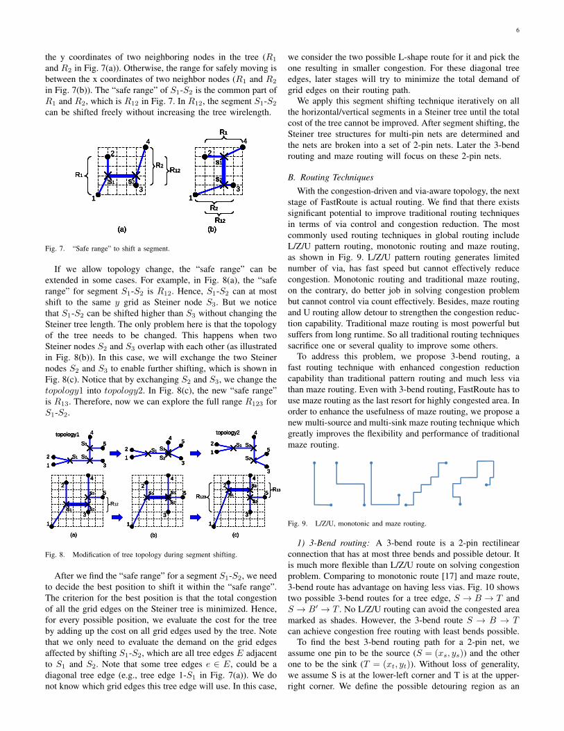
6

the y coordinates of two neighboring nodes in the tree (R1

and R2 in Fig. 7(a)). Otherwise, the range for safely moving isbetween the x coordinates of two neighbor nodes (R1 and R2

in Fig. 7(b)). The “safe range” of S1-S2 is the common part ofR1 and R2, which is R12 in Fig. 7. In R12, the segment S1-S2

can be shifted freely without increasing the tree wirelength.

R1

R2R12

(a)

S1 S2

1

2

3

4R1

R2

R12

(b)

S2

S1

1

2

3

4

R1

R2R12

(a)

S1 S2

1

2

3

4

R1

R2R12

(a)

R2R12

(a)

S1 S2

1

2

3

4R1

R2

R12

(b)

S2

S1

1

2

3

4R1

R2

R12

(b)

S2

S1

R1

R2

R12

(b)

R1

R2

R12

R1

R2

R12

(b)

S2

S1

1

2

3

4

Fig. 7. “Safe range” to shift a segment.

If we allow topology change, the “safe range” can beextended in some cases. For example, in Fig. 8(a), the “saferange” for segment S1-S2 is R12. Hence, S1-S2 can at mostshift to the same y grid as Steiner node S3. But we noticethat S1-S2 can be shifted higher than S3 without changing theSteiner tree length. The only problem here is that the topologyof the tree needs to be changed. This happens when twoSteiner nodes S2 and S3 overlap with each other (as illustratedin Fig. 8(b)). In this case, we will exchange the two Steinernodes S2 and S3 to enable further shifting, which is shown inFig. 8(c). Notice that by exchanging S2 and S3, we change thetopology1 into topology2. In Fig. 8(c), the new “safe range”is R13. Therefore, now we can explore the full range R123 forS1-S2.

R12

S3

S2S1

(a)

1

24

5

3

4

1

2

5

3

S1 S2

S3

topology1

1

24

5

3

R123

R13

(c)

S2

S1

S3

S1

S2

S3

1

2

4

5

3

topology2

S2

S1 S3

(b)

1

24

5

3

S1

S2

S3

1

2

45

3

R12

S3

S2S1

(a)

1

24

5

3

4

1

2

5

3

S1 S2

S3

topology1

S3

S2S1

(a)

1

24

5

3

1

24

5

3

4

1

2

5

3

S1 S2

S3

topology1

1

2

5

3

S1 S2

S3

topology1

1

24

5

3

R123

R13

(c)

S2

S1

S3

S1

S2

S3

1

2

4

5

3

topology2

1

24

5

3

R123

R13

(c)

S2

S1

S3

1

24

5

3

1

24

5

3

R123

R13

(c)

S2

S1

S3

S2

S1

S3

S1

S2

S3

1

2

4

5

3

topology2

S1

S2

S3

1

2

4

5

3

topology2

S2

S1 S3

(b)

1

24

5

3

S1

S2

S3

1

2

45

3

S2

S1 S3

(b)

1

24

5

3

1

24

5

3

S1

S2

S3

1

2

45

3

S1

S2

S3

1

2

45

3

Fig. 8. Modification of tree topology during segment shifting.

After we find the “safe range” for a segment S1-S2, we needto decide the best position to shift it within the “safe range”.The criterion for the best position is that the total congestionof all the grid edges on the Steiner tree is minimized. Hence,for every possible position, we evaluate the cost for the treeby adding up the cost on all grid edges used by the tree. Notethat we only need to evaluate the demand on the grid edgesaffected by shifting S1-S2, which are all tree edges E adjacentto S1 and S2. Note that some tree edges e ∈ E, could be adiagonal tree edge (e.g., tree edge 1-S1 in Fig. 7(a)). We donot know which grid edges this tree edge will use. In this case,

we consider the two possible L-shape route for it and pick theone resulting in smaller congestion. For these diagonal treeedges, later stages will try to minimize the total demand ofgrid edges on their routing path.

We apply this segment shifting technique iteratively on allthe horizontal/vertical segments in a Steiner tree until the totalcost of the tree cannot be improved. After segment shifting, theSteiner tree structures for multi-pin nets are determined andthe nets are broken into a set of 2-pin nets. Later the 3-bendrouting and maze routing will focus on these 2-pin nets.

B. Routing TechniquesWith the congestion-driven and via-aware topology, the next

stage of FastRoute is actual routing. We find that there existssignificant potential to improve traditional routing techniquesin terms of via control and congestion reduction. The mostcommonly used routing techniques in global routing includeL/Z/U pattern routing, monotonic routing and maze routing,as shown in Fig. 9. L/Z/U pattern routing generates limitednumber of via, has fast speed but cannot effectively reducecongestion. Monotonic routing and traditional maze routing,on the contrary, do better job in solving congestion problembut cannot control via count effectively. Besides, maze routingand U routing allow detour to strengthen the congestion reduc-tion capability. Traditional maze routing is most powerful butsuffers from long runtime. So all traditional routing techniquessacrifice one or several quality to improve some others.

To address this problem, we propose 3-bend routing, afast routing technique with enhanced congestion reductioncapability than traditional pattern routing and much less viathan maze routing. Even with 3-bend routing, FastRoute has touse maze routing as the last resort for highly congested area. Inorder to enhance the usefulness of maze routing, we propose anew multi-source and multi-sink maze routing technique whichgreatly improves the flexibility and performance of traditionalmaze routing.

Fig. 9. L/Z/U, monotonic and maze routing.

1) 3-Bend routing: A 3-bend route is a 2-pin rectilinearconnection that has at most three bends and possible detour. Itis much more flexible than L/Z/U route on solving congestionproblem. Comparing to monotonic route [17] and maze route,3-bend route has advantage on having less vias. Fig. 10 showstwo possible 3-bend routes for a tree edge, S → B → T andS → B′ → T . No L/Z/U routing can avoid the congested areamarked as shades. However, the 3-bend route S → B → Tcan achieve congestion free routing with least bends possible.

To find the best 3-bend routing path for a 2-pin net, weassume one pin to be the source (S = (xs, ys)) and the otherone to be the sink (T = (xt, yt)). Without loss of generality,we assume S is at the lower-left corner and T is at the upper-right corner. We define the possible detouring region as an

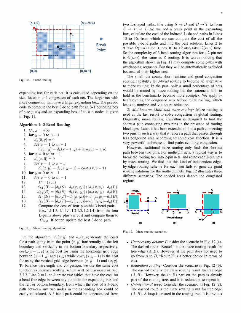
7

B(n‐1,m‐1)(n‐1,0)

T

B

B’Break Point

S

B Point

(0 0) (0 1)(0,0) (0,m‐1)

Fig. 10. 3-bend routing.

expanding box for each net. It is calculated depending on thesize, location and congestion of each net. The larger net withmore congestion will have a larger expanding box. The pseudocode to compute the best 3-bend path for an S-T bounding boxof size p× q and an expanding box of m× n nodes is givenin Fig. 11.

Algorithm 1: 3-Bend Routing1. Cbest = +∞2. for y = 0 to n− 13. dh(0, y) = 04. for x = 1 to m− 15. dh(x, y) = dh(x− 1, y) + costh(x− 1, y)6. for x = 0 to m− 17. dh(x, 0) = 08. for y = 1 to n− 19. dv(x, y) = dv(x, y − 1) + costv(x, y − 1)

10. for y = 0 to n− 111. for x = 0 to m− 112. B = (x, y)13. dL1(B) = |dh(S)−dh(x, ys)|+|dv(x, ys)−dv(B)|14. dL2(B) = |dh(S)−dh(xs, y)|+|dv(xs, y)−dv(B)|15. dL3(B) = |dh(T )−dh(x, yt)|+|dv(x, yt)−dv(B)|16. dL4(B) = |dh(T )−dh(xt, y)|+|dv(xt, y)−dv(B)|17. Compute the cost of four possible 3-bend paths

(i.e., L1-L3, L1-L4, L2-L3, L2-L4) from the fourL-paths above plus via cost and compare them toCbest. If better, update the best 3-bend path.

Fig. 11. 3-bend routing algorithm.

In the algorithm, dh(x, y) and dv(x, y) denote the costsfor a path going from the point (x, y) horizontally to the leftboundary and vertically to the bottom boundary respectively.costh(x− 1, y) is the cost for using the horizontal grid edgebetween (x−1, y) and (x, y) while costv(x, y−1) is the costfor using the vertical grid edge between (x, y− 1) and (x, y).To balance wirelength and congestion, we use the same costfunction as in maze routing, which will be discussed in Sec.3.3.2. Line 2 to Line 9 create two tables that have the cost fora bend-free edge between any points in the expanding box andthe left or bottom boundary, from which the cost of a 3-bendpath between any two nodes in the expanding box could beeasily calculated. A 3-bend path could be concatenated from

two L-shaped paths, like using S → B and B → T to formS → B → T . So we add a break point in the expandingbox, calculate the cost of the induced L-shaped paths in Lines13 to 16, from which we can compute the cost of all thepossible 3-bend paths and find the best solution. Lines 2 to9 take O(mn) time. Lines 10 to 19 also take O(mn) time.So the complexity of 3-bend routing algorithm for a 2-pin netis O(mn), the same as Z routing. It is worth noticing thatthe algorithm shown in Fig. 11 may compute some paths withoverlapping segments. But they will be automatically excludedbecause of their higher cost.

The small via count, short runtime and good congestionsolving capability let 3-bend routing to become an alternativeto maze routing. In the past, only a small percentage of netswould be routed by maze routing but the statement fails tohold as the benchmarks become more complex. We apply 3-bend routing for congested nets before maze routing, whichleads to runtime and via count reduction.

2) Multi-source Multi-sink maze routing: Maze routing isused as the last resort to solve congestion in global routing.Originally, maze routing algorithm is designed to find theshortest path connecting two pins in the presence of routingblockages. Later, it has been extended to find a path connectingtwo pins in such a way that it favors a path that passes throughless congested area according to some cost function. It is avery powerful technique to find paths avoiding congestion.

However, traditional maze routing only finds the shortestpath between two pins. For multi-pin nets, a typical way is tobreak the routing tree into 2-pin nets, and route each 2-pin netsby maze routing. We find that this kind of independent edge-by-edge routing scheme for each net fails to generate goodrouting solutions for the multi-pin nets. Fig. 12 illustrates threedifferent scenarios. The shaded areas denote the congestedregions.

A

Route2

B

C

Route1

D

(a)

A

BC De

Redundancy

(b) (c)

A

BC D

Loop

e

A

Route2

B

C

Route1

D

(a)

A

Route2

B

C

Route1

D

(a)

A

BC De

Redundancy

(b)

A

BC De

Redundancy

(b) (c)

A

BC D

Loop

e

(c)

A

BC D

Loop

e

Fig. 12. Maze routing scenarios.

• Unnecessary detour: Consider the scenario in Fig. 12 (a).The dashed route “Route1” is the maze routing result fortree edge (A,B). However, if the path does not need togo from A to B, “Route2” is a better choice in terms ofcost.

• Redundant routing: Consider the scenario in Fig. 12 (b).The dashed route is the maze routing result for tree edge(A,B). However, the (e,B) part on the path is alreadypart of the routing tree, and it is redundant to repeat it.

• Unintentional loop: Consider the scenario in Fig. 12 (c).The dashed route is the maze routing result for tree edge(A,B). A loop is created in the routing tree. It is obvious

8

that this loop is not needed and only the part from A toe is necessary on the path.

As we can see in these three scenarios, unnecessary wiresare used to route the multi-pin nets. This results in using morerouting resources than necessary and causes extra routing con-gestion. The major defect of this edge-by-edge routing schemefor each net is that the topology information is neglected.When routing a tree edge for multi-pin nets, global routerjust needs to rejoin the two disconnected subtree generated byrip-up procedure, no matter where the rejoining path ends.

A

B

T1 T2

X

Y

A

B

T1 T2

X

Y

Fig. 13. Multi-source multi-sink maze routing.

Aware of the problem, we propose a multi-source multi-sink maze routing algorithm. The main idea is that the existingrouting tree is respected when we route a tree edge for a multi-pin net. We do not constrain the two endpoints of the routingpath to be the original endpoints of the tree edge being routed.As illustrated in Fig. 13, suppose we are routing a tree edge(A,B) in the routing tree T for a multi-pin net N . We firstremove (A,B) from T and obtain two subtrees T1 and T2.(Note that T1 and T2 can be just a point.) We treat all the gridpoints on T1 as sources, and all the grid points on T2 as sinks.Then, we apply the multi-source multi-sink maze routing tofind the best path connecting T1 and T2 to form a tree. In Fig.13, the dotted line from X to Y is the best path to connectT1 and T2.

Our multi-source multi-sink maze routing algorithm isshown in Fig. 14. In the algorithm, d(g) is the distance fromT1 to g, defined as the total cost of all grid edges passed by thetemporary shortest path from T1 to g. The algorithm followsthe framework of Dijkstra’s algorithm [27]. Lines 1-5 initializethe distance d, priority queue Q and destination points. Lines6-17 are the loop similar to Dijkstra’s algorithm. Line 18 justtraces back to find the shortest path from T1 to T2.

Our algorithm finds the least cost routing path from T1 toT2. Theorem 1 gives the optimality of the algorithm.

Theorem 1 The path found by multi-source multi-sink mazerouting algorithm is the least cost routing path from T1 to T2.

Proof: First of all, note that the cost function cost(u, v) isa positive function in our problem. In Line 3, d(u) = 0 for allthe grid points on T1. Hence, we can assume a super sourcewhich replaces all the grid points on T1, and all grid pointsadjacent to T1 are its neighbor. Similarly, we can assume asuper sink which replaces all the grid points on T2, and alladjacent grid points to T2. Then the problem is transformed

Algorithm 2: Multi-source Multi-sink Maze Routing1. d(g) = inf for all grid points g2. Find subtree T1 (contains A) and T2 (contains B) after

removing tree-edge (A,B)3. Set d(u) = 0 and π(u) = nil, for all grid points u on

T14. Set up a priority queue Q with all grid points on T15. Mark all grid points on T2 as sink point6. u← Extract-Min(Q)7. while u is not sink point8. for each neighbor grid point v of u9. if d(v) > d(u) + cost(u, v)

10. π(v) = u11. if v is in Q12. Update Q13. else14. Insert v into Q15. u← Extract-Min(Q)16. Trace back from u using π to find the shortest path from

T1 to T2

Fig. 14. Multi-source multi-sink maze routing algorithm.

to a single-source, single-sink shortest path problem. Theoptimality follows the optimality of Dijkstra’s algorithm.

The only thing left is to prove the stopping criterion iscorrect. Recall that we stop when a destination point on T2is extracted from Q. Assume u is the first destination pointextracted from Q. For the purpose of contradiction, let w bethe destination point which is on the shortest path from T1to T2. Hence, we have d(w) < d(u). However, when weextract u from Q, w is still in Q, which means d(w) ≥ d(u).Because the cost function is positive, d(w) will never decreasein later updating. Therefore, we obtain a contradiction thatd(w) ≥ d(u).

Now we analyze the complexity of the algorithm. Assumethere are V grid points in the search region. Lines 1-5 takestime O(V ). Each Extract-Min operation on the priority queueQ takes time O(lgV ). There are at most V iterations for thewhile loop. For each u, there are at most 4 neighbors adjacentto it. The insertion and updating of Q takes time O(lgV ). Thetotal complexity is therefore O(V lgV ).

We apply this multi-source multi-sink maze routing algo-rithm on the tree edges of multi-pin nets. The runtime ofmaze routing algorithm is highly related to the size of thesearch region. In order to speed up the algorithm, we do notsearch the whole grid graph to find the least cost path. Instead,we use expanding box in the same way as 3-bend routingto significantly reduce the runtime while maintaining goodsolution quality. In our implementation, the enlarge value isproportional to the size and level of congestion of the originalbounding box.

We want to point out one issue for the multi-source multi-sink maze routing technique. It can totally change the routingtree structure because the endpoints of new routing path donot need to be the endpoints of the tree edge being routed.For example, in Fig. 15, the Steiner tree structure is changed

9

from (a) to (b) because of the new routing of tree edge (A,B).Hence, we need to update the Steiner tree structure accordinglyafter routing each tree edge by multi-source multi-sink mazerouting.

A

B

T1

A

B

T2T2

T1

A

B

T1

A

B

T2T2

T1

Fig. 15. Steiner tree topology changed by maze routing.

C. Convergence Enhancement Techniques

In addition to new topology and routing techniques, Fas-tRoute integrates several performance enhancement techniquesto further improve routing quality and reduce run time. Inthe 2007 and 2008 ISPD global routing contests, we find thattraditional global routing framework may easily get trapped inlocal minimal of solution space and require significant runtimeand control to jump out. In order to solve such problem,we propose two new enhancement techniques to improve theconvergence of global routing.

1) Virtual Capacity Technique: Other recently publishedacademic global routers, including BoxRouter [7], Archer [8],NTHU-R [9][10], NTUgr [11] and FGR [12] employ negotia-tion based maze routing technique, which increments the mazerouting cost for consistently congested grid edges. However,such negotiation based cost adjustment lacks theoretical basisand requires significant tuning before it can work properly.

Instead of negotiation based maze routing technique, wepropose virtual capacity, a systematic alternative to handlecongestion problem. Virtual capacity tries to use adjusted“virtual capacity” instead of original capacity to guide mazerouting. Given a global routing solution, consider any con-gested grid edge e. With capacity ue and capacity ce, overflowwould be oe = ue− ce. We denote the virtual capacity as vce.The basic idea of virtual capacity is to reduce the capacityof e by oe units (i.e., set the virtual capacity to ce − oe)for the next round of maze routing. Because of the reductionin capacity, grid edge e becomes more expensive to use andhence some of its routing demand will hopefully be pushedaway. In the ideal situation, exactly oe units of routing demandwill be pushed away in order to bring the congestion back tothe level of the previous round, if we measure the overflowusing virtual capacity. Thus, the new routing demand will beue − oe = ue − (ue − ce) = ce, i.e., the same as the originalcapacity. In order words, grid edge e will not be congestedin the second round of global routing. In reality, more or lessthan oe units of routing demand might be pushed away becauseother grid edges cannot absorb or will absorb more than thepushed routing demand. So it is necessary to update the virtual

capacities and apply maze routing again to further reduce theoverflow.

In Sec. IV-C1a, we discuss the initialization of virtualcapacities. In Sec. IV-C1b, we describe the updating of virtualcapacities during the routing process.

a) Virtual Capacity Initialization by Alternative Conges-tion Estimation (ACE): Virtual capacity is initialized by sub-tracting the overflow of last round of routing from the actualgrid edge capacity. But for the first round of routing, we wantto predict the overflow in order to use virtual capacity to speedup the convergence. We use adaptive congestion estimation(ACE) technique to predict the overflow. ACE assigns netusage to proper grid edge in a more realistic manner andcan estimate overflow much more accurately than traditionalprobabilistic estimation. We implement the estimation usingthe following two assumptions: (1) Routing region of each 2-pin net is confined within the bounding box. (2) Fractionalusage assignment is allowed. The first assumption suggeststhat we only consider the grid edges inside the bounding box.The second assumption allows breaking the integer usage intofractional values. The fractional value models the behaviorof global router that evenly distributes the routing usage incongested region.

The notation of problem formulation of ACE is shownin Table I. ACE designs a more realistic usage assignmentmethod to estimate routing demand. In general, it allocatesthe new routing demand to regions where routing demandsare previously low.

TABLE IACE USAGE ASSIGNMENT NOTATION

N number of 2-pin netsBBoxk bounding box of netk

rk number of rows inside BBoxk

ck number of columns inside BBoxk

leftk left coordinate of BBoxk

rightk right coordinate of BBoxk

topk top coordinate of BBoxk

bottomk bottom coordinate of BBoxk

cV/Hi,j capacity of the e

V/Hi,j

pV/Hi,j current assigned usage of eV/H

i,j

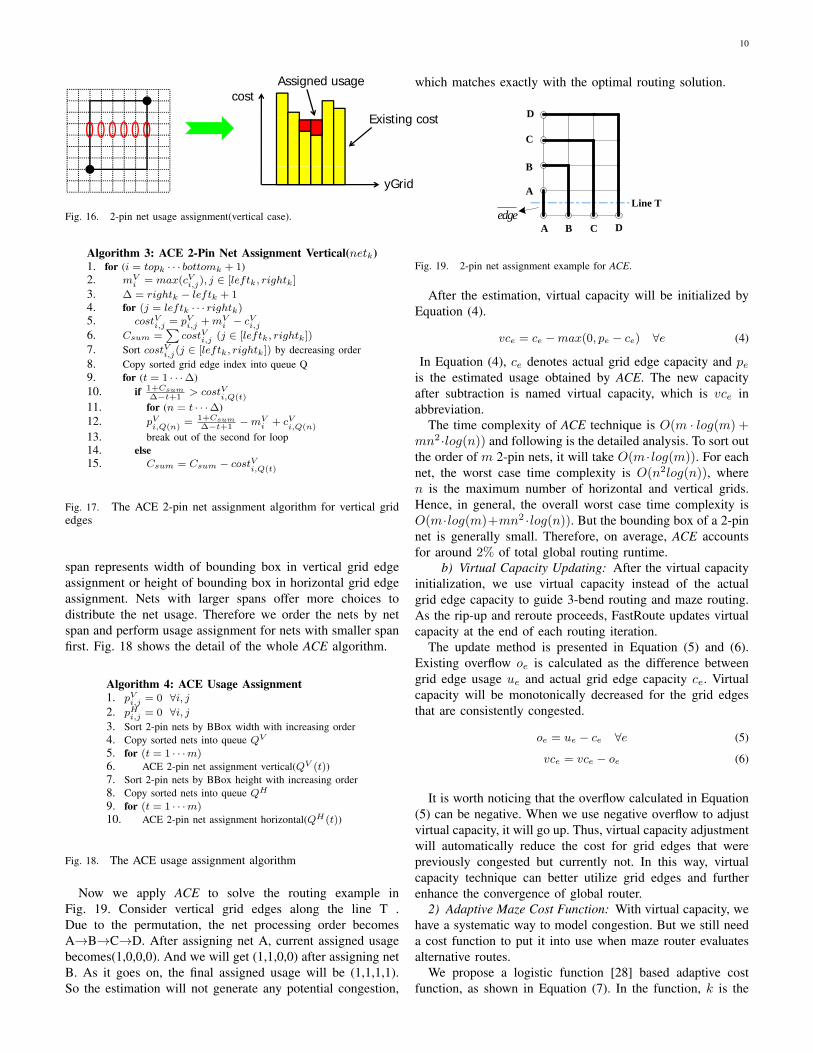
Consider the usage assignment of one single 2-pin net, theusage ready to be assigned within the bounding box is 1.Without loss of generality, here we just discuss the assignmentfor vertical grid edges. The usage assignment algorithm forvertical grid edges is shown in Fig. 17. Each row is processedindependently. Inside one row, grid edges are sorted in adecreasing order according to the value of costVi,j , which isequal to pVi,j + mV

i − cVi,j . mVi is the value of maximum

grid edge capacity of row i. The algorithm compares theaverage potential assigned usage with largest current assignedusage. It iteratively excludes the grid edge with largest currentassigned usage until an even assignment is possible. The timecomplexity required for processing single 2-pin net netk isO(rkck · log(ck)). Fig. 16 illustrates the assignment process.

Due to the sequential manner of usage assignment, thenet processing order may significantly affect accuracy. ACEprocesses smaller span nets with higher priority. The net

10

costAssigned usage

Existing costExisting cost

yGrid

2

Fig. 16. 2-pin net usage assignment(vertical case).

Algorithm 3: ACE 2-Pin Net Assignment Vertical(netk)1. for (i = topk · · · bottomk + 1)2. mV

i = max(cVi,j), j ∈ [leftk, rightk]

3. ∆ = rightk − leftk + 14. for (j = leftk · · · rightk)

5. costVi,j = pVi,j + mVi − cVi,j

6. Csum =∑

costVi,j (j ∈ [leftk, rightk])

7. Sort costVi,j(j ∈ [leftk, rightk]) by decreasing order8. Copy sorted grid edge index into queue Q9. for (t = 1 · · ·∆)10. if 1+Csum

∆−t+1> costV

i,Q(t)

11. for (n = t · · ·∆)12. pV

i,Q(n)= 1+Csum

∆−t+1−mV

i + cVi,Q(n)

13. break out of the second for loop14. else15. Csum = Csum − costV

i,Q(t)

Fig. 17. The ACE 2-pin net assignment algorithm for vertical gridedges

span represents width of bounding box in vertical grid edgeassignment or height of bounding box in horizontal grid edgeassignment. Nets with larger spans offer more choices todistribute the net usage. Therefore we order the nets by netspan and perform usage assignment for nets with smaller spanfirst. Fig. 18 shows the detail of the whole ACE algorithm.

Algorithm 4: ACE Usage Assignment1. pVi,j = 0 ∀i, j2. pHi,j = 0 ∀i, j3. Sort 2-pin nets by BBox width with increasing order4. Copy sorted nets into queue QV

5. for (t = 1 · · ·m)

6. ACE 2-pin net assignment vertical(QV (t))7. Sort 2-pin nets by BBox height with increasing order8. Copy sorted nets into queue QH

9. for (t = 1 · · ·m)

10. ACE 2-pin net assignment horizontal(QH(t))

Fig. 18. The ACE usage assignment algorithm

Now we apply ACE to solve the routing example inFig. 19. Consider vertical grid edges along the line T .Due to the permutation, the net processing order becomesA→B→C→D. After assigning net A, current assigned usagebecomes(1,0,0,0). And we will get (1,1,0,0) after assigning netB. As it goes on, the final assigned usage will be (1,1,1,1).So the estimation will not generate any potential congestion,

which matches exactly with the optimal routing solution.

Line TA

A B

B

C

C

D

Dedge

Fig. 19. 2-pin net assignment example for ACE.

After the estimation, virtual capacity will be initialized byEquation (4).

vce = ce −max(0, pe − ce) ∀e (4)

In Equation (4), ce denotes actual grid edge capacity and peis the estimated usage obtained by ACE. The new capacityafter subtraction is named virtual capacity, which is vce inabbreviation.

The time complexity of ACE technique is O(m · log(m) +mn2·log(n)) and following is the detailed analysis. To sort outthe order of m 2-pin nets, it will take O(m · log(m)). For eachnet, the worst case time complexity is O(n2log(n)), wheren is the maximum number of horizontal and vertical grids.Hence, in general, the overall worst case time complexity isO(m·log(m)+mn2 ·log(n)). But the bounding box of a 2-pinnet is generally small. Therefore, on average, ACE accountsfor around 2% of total global routing runtime.

b) Virtual Capacity Updating: After the virtual capacityinitialization, we use virtual capacity instead of the actualgrid edge capacity to guide 3-bend routing and maze routing.As the rip-up and reroute proceeds, FastRoute updates virtualcapacity at the end of each routing iteration.

The update method is presented in Equation (5) and (6).Existing overflow oe is calculated as the difference betweengrid edge usage ue and actual grid edge capacity ce. Virtualcapacity will be monotonically decreased for the grid edgesthat are consistently congested.

oe = ue − ce ∀e (5)

vce = vce − oe (6)

It is worth noticing that the overflow calculated in Equation(5) can be negative. When we use negative overflow to adjustvirtual capacity, it will go up. Thus, virtual capacity adjustmentwill automatically reduce the cost for grid edges that werepreviously congested but currently not. In this way, virtualcapacity technique can better utilize grid edges and furtherenhance the convergence of global router.

2) Adaptive Maze Cost Function: With virtual capacity, wehave a systematic way to model congestion. But we still needa cost function to put it into use when maze router evaluatesalternative routes.

We propose a logistic function [28] based adaptive costfunction, as shown in Equation (7). In the function, k is the

11

coefficient controlling the function curve slope when ue isbelow ce. k is adaptively adjusted in different maze routingphases. In the initial phase, k is set small to preserve goodwirelength. Normally in the first few iterations, many netsneed rip-up and reroute. If a large k coefficient is applied,those nets would be rerouted with huge detour. While in thefinal stage of maze routing, the cost function curve is madesteep to aggressively drive down the residual overflow. Thereare two other coefficients in the function: S determines theslope when ue is over ce. H is the cost height which controlsthe trade off between converging speed and wirelength andwould be increased each maze routing iteration.

coste =

{1 +H/(1 + exp(−k(ue − vce))) if 0 < ue ≤ ce

1 +H + S × (ue − vce) if ue > ce(7)

D. Spiral Layer Assignment

There are generally two ways to generate solutions for 3Dglobal routing benchmarks. One is running routing techniquesand layer assignment concurrently. It overly complicates theproblem and is rarely used. The other more popular wayfirst projects the 3D benchmarks from aerial view, finds asolution for the 2D problem and expands the solution tomultiple layers. This expansion is called layer assignment,which has significant impact on the number of vias for thefinal solution. To keep FastRoute fast, we propose a sequentiallayer assignment algorithm that would assign the 2D solutioninto routing layers, from lower layers to higher ones. Thelayer assignment algorithm will not change the aerial view of2D solution and thus keep the total wirelength. Besides, ouralgorithm keeps total number of overflow unchanged. Thus,if we can find a congestion-free solution for the 2D globalrouting problem, we can find a valid solution for the original3D problem.

In the algorithm, we first sort the nets considering theirtotal wirelength and number of pin nodes. Then we orderthe segments in each net according to their locations in thenet. Finally, we assign layers using dynamic programming,segment by segment, net by net.

Due to the competition of different nets in the assigningsequence and greedy nature of layer assignment, careless earlyassignment causes later nets switching among the layers andthus generates a large number of unnecessary vias. Smallernets connecting nearby global cells are considered relativelylocal and should use lower metal layers. On the contrary,longer nets assigned to upper layers will encounter less switch-ing between layers and will use wider tracks on top layers toachieve better timing. Furthermore, we observe that nets withhigher number of pins tend to cause more vias. So we ordernets by an increasing order of

∑wl/#Pins, where

∑wl is

the total wirelength for a net. Thus, we keep nets with smallertotal wirelength and higher pin count on the lower layers.

For each net, we order segments for the following reason.The only layer information for a net is that the pin nodes mustgo up to at least metal layer 1 to have metal connections. Sowe order the segments in each net in increasing order of their

distance to the pin nodes. Here, the distance is defined asthe number of segments the two nodes in a segment have totraverse to reach the nearest pin node. We first assign layers tothe segments with 0 distance i.e., segments that have at leastone pin node and move onto segments with larger distance.By such an order, we are sure that at least one end of eachsegment has the information that which layers the pin noderanges between. Thus, we start assigning segments on theperiphery of a net and continue inwardly.

As shown in Fig. 20, we create a “via grid graph” to assigneach segment to metal layers. We call each node on the grapha “via node”. Vertical grid edges represent the possible placesto add via while the horizontal grid edges are constructed fromthe actual 2D path in the “via grid graph”. We pull straightthe original zigzagged 2-pin net to form the horizontal gridedges in the via grid graph and copy the capacity and usageof corresponding grid edge from the original grid graph. Webreak the segments in a tree into the size of grid edges andassign them to layers one by one. Such breakdown enablesus to keep the total number of wirelength and overflow of the2D solution unchanged. Without loss of generality, we assumesources Si on the very left column and targets Tj on the right.If we do not know the layer information about the endingnode, layer 1 to L are all considered to be targets. Here, Lis the number of metal layers in a benchmark. Otherwise, thetarget is set to be the spanning range of the ending node.

T6M6T56

T

M5

M4

M6

T3

T4

M3

M4

S2

T3

T2

M3

M22

S1 T1M1

Fig. 20. Dynamic programming layer assignment.

We associate every via node with a cost, which representsthe least number of vias on the paths from the node to anysource nodes. Since we do not change the aerial view of a net,a 3D path must and must only use the horizontal segmentsbetween two adjacent columns once. Thus, the cost for anode is the same as its left neighbor if there is still routingresource or one plus the cost associated with the upper orlower neighbor nodes, whichever is smaller. The pseudo-codeto process each segment with wirelength n is shown in Fig.21.

In the algorithm, Line 1 uses O(nL) time and Line 2 takesO(L) time. The update of costs from vertical neighbors in-volves with a series of sorting, comparison and update, whichtakes O(LlgL) time. However, because of the small numberof L (typically less than 10 depending on the semiconductorprocess), we use an O(L2) implementation. Hence, Line 4 toLine 8 take O(nL2). So the complexity of layer assignmentfor each segment is O(nL2).

12

Algorithm 5: Layer Assignment for Segment1. Initialize the cost for all the via nodes to +∞2. For every source sj , C(j, 0) = 03. Update the cost for other via nodes on the first column4. for x = 1 to n− 15. for j = 1 to L6. if cap(j, x− 1) > usg(j, x− 1)7. C(j, x) = C(j, x− 1)8. Update the cost from vertical neighbors.9. Find the least cost for any sink node and trace back

using C(j, x)

Fig. 21. Layer assignment algorithm for segment.

V. EXPERIMENTAL RESULTS

We implemented FastRoute in C with Steiner tree packageFLUTE and the current version is FastRoute 4.1. All theexperiments are performed on a Linux machine with 2.8GHz Intel processor and 32GB RAM. We run experiments onISPD08 global routing contest benchmarks [30]. The bench-mark statistics are shown in table II. It is worth mentioningthat FastRoute 4.1 now adopts a single set of tuning and avoidsspecific benchmark tuning to demonstrate the effectivenessof global routing framework and techniques presented in thiswork. On the contrary, all the participants in ISPD 08 contestuse benchmark specific tuning.

The 2008 set of benchmarks has 8 new benchmarks and8 benchmarks inherited from 2007. However, when ISPD08global routing contest considers one unit of via at the samecost of one unit of wirelength, the one held in 2007 chargesvia at a cost three times of the cost for wirelength. In ourexperiment, we use the rules set by the 2008 contests whichtreats wire segments and vias equally.

In Table III., we compare the performance of FastRoute4.1 on the ISPD08 global routing contest benchmarks withthe top 4 routers besides FastRoute 3.0. Again, FastRoute4.1 is the fastest router. For the four benchmarks that no onecan successfully finish routing without incurring any overflow,FastRoute achieves lowest overflow for two benchmarks. Dueto the fact that other groups do not disclose the details aboutthe metal wirelength part and via part of the total wirelength,we only compare the total wirelength. Since no newer datais available for BoxRouter2.0 after the ISPD08 contest, wequote the results for BoxRouter2.0 from ISPD08 global routingcontest results. All runtime are scaled to 2.8GHz.

Comparing to NTHU-R2.0, the 2008 ISPD global routingcontest winner, FastRoute achieves 0.01% and 74% improve-ment for total wirelength and runtime respectively on the 12routable benchmarks. Comparing to the 2nd place winner,NTUgr, FastRoute 4.1 can finish routing one more benchmarkwithout overflow and can achieve 3.8% less wirelength in15X faster speed for 11 benchmarks that the two routers bothsuccessfully finished.

1Segment wirelength, via and total wirelength are in unit of 10K.2Wirelength and runtime comparisons are based on overflow-free bench-

marks.

Via accounts for 26% to 47% of the total wirelength ofFastRoute solutions to the contest benchmarks. Although viahas higher resistivity and larger process variation which makesit much more important than before, we still believe thatcongestion reduction is the most important function for globalrouter. Both of the two recent global routing contests held byISPD gave highest priority to the overflow of solutions forevaluating the performance of global routers.

Even though most global router that participated in the 2008ISPD global routing contests have greatly improved over theirearlier version in the 2007 contest, we observe that somerouters still face two challenges. One is how to handle thecongestion left in the final stages. Even though FastRoute 4.1and NTHU-R2.0 successfully finished routing for newblue1,they both failed newblue4, newblue7 and bigblue4, with aresidue overflow of just less than 150. The huge runtimespent by NTUgr and BoxRouter2.0 on newblue1 showed theinability to solve the few final overflow. Another challengeis the effectiveness for the global routers to balance betweenreducing the number of overflow and extending wirelength.The conflict incurs due to the fact that one of the mostefficient method to reduce congestion is detour, i.e. extendingwirelength, which could however induce congestion in otherareas. One important way to effectively control the trade-offis through cost function used in maze routing. Although costfunctions evolve from step function to logistic function andthe variants of logistic functions, the fact that global routersthat generates shorter wirelength or longer wirelength can onlyreduce congestion to a similar level demonstrates that thereis considerable potential for the academic global routers toimprove in this area.

To demonstrate the effectiveness of the global routing tech-niques proposed in this paper, we turn off certain techniquesto see the performance degradation as shown in Table IV. Inthe column “No Tree Adj”, we turn off the congestion-drivenvia-aware Steiner tree generation and use unadjusted treetopology directly generated from FLUTE. This configurationof FastRoute leads to 38% more congestion and 23% run timeoverhead. The “No 3-Bend” column shows the performanceof FastRoute without 3-Bend routing. We observe degradationfor all three qualities we focus on, though the degradationare not very significant. However, FastRoute spends 55%more runtime for the four unroutable benchmarks without 3-Bend routing, which has explanation in the fact that 3-bendrouting is much more efficient than maze routing. The “NoVCA” column shows results generated by FastRoute withoutVirtual Capacity Adjustment. Without convergence assistingtechniques, FastRoute only finishes 5 benchmarks withoutoverflow. This configuration also dramatically increase totalwirelength and runtime because FastRoute spends much moretime running maze routing to try to eliminate overflow. Forthe last configuration, we turn off net ordering and segmentordering used in the spiral layer assignment and it showsthat the two ordering saves 11% of wirelength, which wouldtranslate into significantly more percentages of via.

3Wirelength and runtime comparisons are based on overflow-free bench-marks.

13

TABLE IIEXPERIMENTAL BENCHMARKS STATISTICS

#Routed Max AvgName Grids #Layers #Nets Nets Deg Deg

adaptec1 324×324 6 219K 177k 340 4.2adaptec2 424×424 6 260K 208k 153 3.9adaptec3 774×779 6 466K 368k 82 4.0adaptec4 774×779 6 515K 401k 171 3.7adaptec5 465×468 6 867K 548k 121 4.1newblue1 399×399 6 332K 271k 74 3.5newblue2 557×463 6 463K 374k 116 3.6newblue3 973×1256 6 552K 442k 141 3.2newblue4 455×458 6 636K 531k 152 3.6newblue5 637×640 6 1.26M 892k 258 4.1newblue6 463×464 6 1.29M 835k 123 3.8newblue7 488×490 8 2.64M 1.65M 113 3.6bigblue1 227×227 6 283K 197k 74 4.1bigblue2 468×471 6 577K 429k 260 3.5bigblue3 555×557 8 1.12M 666k 91 3.4bigblue4 403×405 8 2.23M 1.13M 129 3.7

TABLE IIIFASTROUTE 4.1 RESULTS ON 3D VERSION OF ISPD08 GLOBAL ROUTING CONTEST BENCHMARKS

FastRoute 4.1 NTHU-R2.0 [10] NTUgr [11] BoxRouter2.0 [30]name ovfl swl1 via1 twl1 cpu(s) ovfl twl1 cpu(s) ovfl twl1 cpu(s) ovfl twl1 cpu(s)

adaptec1 0 36.4 17.4 53.8 193 0 53.4 568 0 57.4 270 0 52.9 1227adaptec2 0 33.3 18.9 52.2 51 0 52.3 98 0 53.7 66 0 52.7 162adaptec3 0 96.7 34.5 131.2 183 0 131.0 510 0 135.0 264 0 131.8 1635adaptec4 0 89.9 31.4 121.3 61 0 121.7 121 0 123.7 72 0 122.1 403adaptec5 0 104.1 51.7 155.8 407 0 155.4 1077 0 159.9 918 0 156.9 1889newblue1 0 24.5 21.8 46.3 361 0 46.5 290 6 49.3 58650 44 47.5 74488newblue2 0 46.7 28.5 75.2 40 0 75.7 57 0 76.9 36 0 75.9 109newblue3 31532 76.5 31.3 107.8 1353 31454106.5 5728 31024188.353040 38958 109.1 82615newblue4 142 82.9 47.6 130.5 2140 138 130.5 4525 142 143.867086 200 129.5 78225newblue5 0 148.8 82.1 230.9 565 0 231.6 908 0 244.9 1230 0 232.9 1700newblue6 0 103.7 73.8 177.5 598 0 176.9 847 0 186.6 1278 0 179.8 1785newblue7 54 186.1166.8352.916888 62 353.5 6734 310 372.286730 208 358.6 84743bigblue1 0 37.9 18.7 56.6 257 0 56.0 641 0 60.0 918 0 56.9 1147bigblue2 0 49.3 41.6 90.9 457 0 90.6 397 0 91.2 14898 0 90.4 2346bigblue3 0 78.9 51.1 130.0 114 0 130.7 235 0 133.5 240 0 131.3 380bigblue4 138 121.3108.9230.2 2144 162 231.0 6159 188 242.824786 472 231.6 52644

Comparison2 1 \ \ 1 1 0.998 1.001 1.75 0.994 1.038 23.99 1.25 1.0007 26.55

TABLE IVCONTRIBUTIONS FROM TECHNIQUES IN FASTROUTE

FastRoute 4.1 No Tree Adj No 3-Bend No VCA Input Order LAname ovfl twl cpu(s) ovfl twl cpu(s) ovfl twl cpu(s) ovfl twl cpu(s) ovfl twl cpu(s)

adaptec1 0 53.8 193 0 54.1 211 0 54.2 192 0 54.4 941 0 58.6 176adaptec2 0 52.2 51 0 52.4 56 0 52.4 58 126 52.8 343 0 56.7 37adaptec3 0 131.2 183 0 131.8 195 0 132.2 189 0 130.5 384 0 140.5 155adaptec4 0 121.3 61 0 121.5 60 0 121.3 62 0 121.3 70 0 129.4 30adaptec5 0 155.8 407 0 156.5 448 0 157.1 457 0 171.6 315 0 171.6 315newblue1 0 46.3 361 0 46.4 335 0 46.4 313 1362 46.6 2431 0 52.2 299newblue2 0 75.2 40 0 75.4 46 0 75.1 40 0 75.2 41 0 83.0 15newblue3 31532107.8 1353 33628107.8 3895 38563107.5 4345 34528108.5 4679 31532114.3 3737newblue4 142 130.5 2140 146 130.9 2211 144 130.9 2644 1352 130.512940 142 139.9 2189newblue5 0 230.9 565 0 231.9 646 0 232.2 670 166 235.620244 0 254.8 446newblue6 0 177.5 598 0 179.0 703 0 179.2 668 42 180.2 4755 0 202.1 514newblue7 54 352.916888 80 354.817376 86 353.322284 1124 357.142598 54 403.312633bigblue1 0 56.6 257 0 57.2 300 0 57.0 383 84 57.2 2179 0 63.6 231bigblue2 0 90.8 457 0 91.1 516 0 91.1 762 48 91.6 2355 0 99.1 434bigblue3 0 130.1 114 0 130.2 115 0 130.4 242 268 131.3 3195 0 150.0 73bigblue4 138 230.2 2144 144 232.1 4059 142 231.5 5529 648 228.9 7177 138 265.5 2807

Comparison3 1 1 1 1.38 1.005 1.23 1.07 1.004 1.10 1.25 1.02 11.33 1 1.11 0.83

14

The source code of lastest FastRoute 4.1 could be re-quested for download at http://home.eng.iastate.edu/cnchu/FastRoute.html. If the reader is interested, one can find allthe algorithm and tuning factors inside. The latest FastRoute4.1 uses a single set of tuning factors. The major factors arebounding box sizes, maze routing iterations and the factorsused in formula 7 in the cost funciton. Due to space limit, weonly present the philosophy in how to set them and user canrefer to the source code to find the exact value. For boudingbox sizes, Fastroute starts at a small value to limit detour atthe beginning of routing process. It increases as maze routingiterations proceed but is capped at 20% of the entire gridgraph size because a larger bounding box would not help tofurther eliminate congestion and would increase runtime invain. FastRoute run maze routing for at most 100 iterationsor as soon as it elimiates all violation. For the coefficient informula 7, H keeps growing to increase the strength to pushaway nets from congested edges. S is set to 10

VI. CONCLUSION

In this paper, we develop a new global routing tool thatfocuses on reducing routing congestion and the number ofvias. If the runtime bonus used in ISPD08 is considered, Fas-tRoute 4.1 outperforms every single academic global router.In addition, it reduces the via count significantly during globalrouting.

Our future work will focus on how to control maze routingso that it can make more effective balance between reducingcongestion and keeping wirelength small.

REFERENCES

[1] [1] J. Hu and S. S. Sapatnekar, “A survey on multi-net global routingfor integrated circuits,” Integration, the VLSI Journal, vol. 31, no. 1, pp.1-49, 2001.

[2] [2] M. D. Moffitt, J. A. Roy and I. L. Markov, “The coming of age of(academic) global routing,” invited paper Proc. of Intl. Symp. on PhysicalDesign, pp 148-155, 2008.

[3] [3] C.Albrecht, “Global routing by new approximation algorithms formulticommodity flow,” IEEE trans. on Computer-Aided Design of Inte-grated Circuits and Systems, vol. 20, no. 5, pp. 622-631, 2001.

[4] [4] M. Cho and D. Z. Pan, “BoxRouter: A new global router based on boxexpansion and progressive ILP,” Proc. of Design Automation Conference,pp. 373-378, 2006.

[5] [5] R. Kastner, E. Bozorgzadeh and M. Sarrafzadeh, “Pattern Routing:Use and Theory for Increasing Predictability and Avoiding Coupling,”IEEE trans. on Computer-Aided Design of Integrated Circuits and Sys-tems, vol. 21, no. 7, pp. 777-790, 2002.

[6] [6] R.T. Hadsell and P.H. Madden, “Improved global routing throughcongestion estimation,” Proc. of Design Automation Conference, pp. 28-31, 2003.

[7] [7] M. Cho, K. Lu, K. Yuan and D. Z. Pan, “BoxRouter 2.0: Architectureand Implementation of a hybrid and robust global router,” Proc. of Intl.Conf. on Compuer-Aided Design, pp. 503-508, 2007.

[8] [8] M. M. Ozdal and M. D.F. Wong, “ARCHER: a history-driven globalrouting algorithm,” Proc. of Intl. Conf. on Computer-Aided Design, pp.481-487, 2007.

[9] [9] J.-R. Gao, P.-C. Wu, and T.-C. Wang, “A new global router for moderndesigns,” Proc. Asia and South Pacific Design Automation Conf., 2008.

[10] [10] Y.-J. Chang, Y.-T. Lee, and T.-C. Wang, “NTHU-Route 2.0: A Fastand Stable Global Router,” Proc. IEEE/ACM Intl. Conf. on Compuer-Aided Design, 2008.

[11] [11] Y. Chen, C. Hsu and Y. Chang“High-Performance Global Routingwith Fast Overflow Reduction,” Proc. Asia and South Pacific DesignAutomation Conf., 2009.

[12] [12] J. A. Roy and I. L. Markov, “High-performance routing at thenanometer scale,” Proc. IEEE/ACM Intl. Conf. on Compuer-Aided Design,pp. 496-502, 2007.

[13] [13] L. McMurchie and C. Ebeling, “Pathfinder: A negotiation-basedperformance-driven router for FPGAs,” Proc. of Int’l Symp. on Field-Programmable Gate Arrays, pp. 111-117, 1995.

[14] [16] M. D. Moffitt, “MaizeRouter: Engineering an effective globalrouter,” Proc. Asia and South Pacific Design Automation Conf., 2008.

[15] [17] J. A. Roy and I. L. Markov, “High-performance Routing at theNanometer Scale,” IEEE trans. on Computer-Aided Design of IntegratedCircuits and Systems, VOL. 27, NO. 6, pp. 1066-1077, 2008.

[16] [14] M. Pan and C. Chu, “FastRoute: A step to integrate global routinginto placement,” Proc. of Intl. Conf. on Computer-Aided Design, pp. 464-471, 2006.

[17] [15] M. Pan and C. Chu, “FastRoute 2.0: A high-quality and efficientglobal router,” Proc. of Asia and South Pacific Design Automation Conf.,2007.

[18] [18] Y. Zhang, Y. Xu and C. Chu, “FastRoute 3.0: a fast and high qualityglobal router based on virtual capacity,” Proc. IEEE/ACM Intl. Conf. onComputer-Aided Design, pp. 344-349, 2008.

[19] [18] Y. Xu, Y. Zhang and C. Chu, “FastRoute 4.0: global routerwith efficient via minimization,” Proc. Asia and South Pacific DesignAutomation Conf., 2009.

[20] [19] T. Wu, A. Davoodi and J. Linderoth, “GRIP: scalable 3D globalrouting using integer programming,” Proc. of Design Automation Confer-ence, pp. 320-325, 2009.

[21] [20] C. Chu, “FLUTE: Fast lookup table based wirelength estimationtechnique,” Proc. of Intl. Conf. on Compuer-Aided Design, pp. 696-701,2004.

[22] [21] C. Chu and Y.-C. Wong “FLUTE: Fast lookup table based recti-linear Steiner minimal tree algorithm for VLSI design,” IEEE Trans. onComputer-Aided Design of Integrated Circuits and Systems, vol. 27, no.1, pp. 70-83, 2008.

[23] [22] J. Cong, M. Xie and Y. Zhang, “MARS - A multilevel fullchipgridless routing system,” IEEE Trans. on Computer-Aided Design ofIntegrated Circuits and Systems, vol. 24, no. 3, pp. 382-394, 2005.

[24] [23] J. Westra, C. Bartels and P. Groeneveld, “Probabilistic congestionprediction,” Proc. of Intl. Symp. on Physical Design, pp 204-209, 2004.

[25] [24] J. Westra and P. Groeneveld, “Is probabilistic congestion estimationworthwhile?” Proc. Intl. Workshop on System-Level Interconnect Predic-tion(SLIP), pp. 99-106, 2005.

[26] [25] M. Hanan, “On Steiner’s problem with rectilinear distance,” SIAMJournal of Applied Mathematics, vol. 14, pp. 255-265, 1966.

[27] [26] E. Dijkstra, “A note on two problems in connexion with graphs,”Numerische Mathematik, vol. 1, pp. 269-271, 1959.

[28] [27] D. von Seggern. CRC Standard Curves and Surfaces. Boca Raton,FL: CRC Press, 1993.

[29] [28] http://www.sigda.org/ispd2007/rcontest/.[30] [29] http://www.ispd.cc/contests/ispd08rc.html.