Faster Gaze Prediction With Dense Networksand Fisher Pruning

Lucas Theis, Iryna Korshunova, Alykhan Tejani, and Ferenc Huszar{ltheis,ikorshunova,atejani,fhuszar}@twitter.com

Twitter

Abstract. Predicting human fixations from images has recently seenlarge improvements by leveraging deep representations which were pre-trained for object recognition. However, as we show in this paper, thesenetworks are highly overparameterized for the task of fixation prediction.We first present a simple yet principled greedy pruning method whichwe call Fisher pruning. Through a combination of knowledge distillationand Fisher pruning, we obtain much more runtime-efficient architecturesfor saliency prediction, achieving a 10x speedup for the same AUC per-formance as a state of the art network on the CAT2000 dataset. Speedingup single-image gaze prediction is important for many real-world appli-cations, but it is also a crucial step in the development of video saliencymodels, where the amount of data to be processed is substantially larger.

1 Introduction

The ability to predict the gaze of humans has many applications in computervision and related fields. It has been used for image cropping [1], improving videocompression [2], and as a tool to optimize user interfaces [3], for instance. In psy-chology, gaze prediction models are used to shed light on how the brain mightprocess sensory information [4]. Recently, due to advances in deep learning, hu-man gaze prediction has received large performance gains. In particular, reusingimage representations trained for the task of object recognition have proven tobe very useful [5,6]. However, these networks are relatively slow to evaluate whilemany real-world applications require highly efficient predictions. For example,popular websites often deal with large amounts of images which need to be pro-cessed in a short amount of time using only CPUs. Similarly, improving videoencoding with gaze prediction maps requires the processing of large volumes ofdata in near real-time.

In this paper we explore the trade-off between computational complexityand gaze prediction performance. Our contributions are two-fold: First, usinga combination of knowledge distillation [7] and pruning, we show that goodperformance can be achieved with a much faster architecture, achieving a 10xspeedup for the same generalization performance in terms of AUC. Secondly,we provide a principled derivation for the pruning method of Molchanov et al.[8], extend it, and show that our extension works well when applied to gaze

arX

iv:1

801.

0578

7v2

[cs

.CV

] 9

Jul

201

8

2

prediction. We further discuss how to choose the trade-off between performanceand computational cost and suggest methods for automatically tuning a weightedcombination of the corresponding losses, reducing the need to run expensivehyperparameter searches.

2 Fast Gaze Prediction Models

Our models build on the recent state-of-the-art model DeepGaze II [6], whichwe first review before discussing our approach to speeding it up. The backboneof DeepGaze II is formed by VGG-19 [9], a deep neural network pre-trained forobject recognition. Feature maps are extracted from several of the top layers,upsampled, and concatenated. A readout network with 1 × 1 convolutions andReLU nonlinearities [10] takes in these feature maps and produces a single outputchannel, implementing a point-wise nonlinearity. This output is then blurredwith a Gaussian filter, Gσ, followed by the addition of a center bias to take intoaccount the tendencies of observers to fixate on pixels near the image center. Thiscenter bias is computed as the marginal log-probability of a fixation landing on agiven pixel, logQ(x, y), and is dataset dependent. Finally, a softmax operation isapplied to produce a normalized probability distribution over fixation locations,or saliency map:

Q(x, y | I) ∝ exp (R(U(F (I))) ∗Gσ + logQ(x, y)) (1)

Here, I is the input image, F extracts feature maps, U bilinearly upsamples thefeature maps and R is the readout network.

To improve efficiency, we made some minor modifications in our reimplemen-tation of DeepGaze II. We first applied the readout network and then bilinearlyupsampled the one-dimensional output of the readout network, instead of up-sampling the high-dimensional feature maps. We also used separable filters forthe Gaussian blur. To make sure the size of the saliency map matches the size ofthe input image, we upsample and crop the output before applying the softmaxoperation.

We use two basic alternative architectures providing different trade-offs be-tween computational efficiency and performance. First, instead of VGG-19, weuse the faster VGG-11 architecture [9]. As we will see, the performance lost byusing a smaller network can for the most part be compensated by fine-tuning thefeature map representations instead of using fixed pre-trained representations.Second, we try DenseNet-121 [11] as a feature extractor. DenseNets have beenshown to be more efficient, both computationally and in terms of parameterefficiency, when compared to state-of-the-art networks in the object recognitiontask [11].

Even when starting from these more parameter efficient pre-trained models,the resulting gaze prediction networks remain highly over-parametrized for thetask at hand. To further decrease the number of parameters we turn to pruning:greedy removal of redundant parameters or feature maps. In the following sectionwe derive a simple, yet principled, method for greedy network pruning which wecall Fisher pruning.

3

2.1 Fisher Pruning

Our goal is to remove feature maps or parameters which contribute little to theoverall performance of the model. In this section, we consider the general caseof a network with parameters θ trained to minimize a cross-entropy loss,

L(θ) = EP [− logQθ(z | I)] , (2)

where I are inputs, z are outputs, and the expectation is taken with respect tosome data distribution P . We first consider pruning single parameters θk. Forany change in parameters d, we can approximate the corresponding change inloss with a 2nd order approximation around the current parameter value θ:

g = ∇L(θ), H = ∇2L(θ), (3)

L(θ + d)− L(θ) ≈ g>d +1

2d>Hd (4)

Following this approximation, dropping the kth parameter (setting θk = 0)would lead to the following increase in loss:

L(θ − θkek)− L(θ) ≈ −gkθk +1

2Hkkθ

2k, (5)

where ek is the unit vector which is zero everywhere except at its kth entry,where it is 1. Following related methods which also start from a 2nd orderapproximation [12,13], we assume that the current set of parameters is at a localoptimum and that the 1st term vanishes as we average over a dataset of inputimages. In practice, we found that including the first term actually reduced theperformance of the pruning method. For the diagonal of the Hessian, we use theapproximation

Hkk ≈ EP

[(∂

∂θklogQθ(z | I)

)2], (6)

which assumes that Qθ(z | I) is close to P (z | I) (see Supplementary Section 1for a derivation). Eqn. (6) can be viewed as an empirical estimate of the Fisherinformation of θk, where an expectation over the model is replaced with real datasamples. If Q and P are in fact equal and the model is twice differentiable withrespect to parameters θ, the Hessian reduces to the Fisher information matrixand the approximation becomes exact.

If we useN data points to estimate the Fisher information, our approximationof the increase in loss becomes

∆k =1

2Nθ2k

N∑n=1

g2nk, (7)

where gn is the gradient of the parameters with respect to the nth data point.In what follows, we are going to use this as a pruning signal to greedily removeparameters one-by-one where this estimated increase in loss is smallest.

4

For convolutional architectures, it makes sense to try to prune entire featuremaps instead of individual parameters, since typical implementations of convo-lutions may not be able to exploit sparse kernels for speedups. Let ankij be theactivation of the kth feature map at spatial location i, j for the nth datapoint.Let us also introduce a binary mask m ∈ {0, 1}K into the network which modifiesthe activations ankij of each feature map k as follows:

ankij = mkankij . (8)

The gradient of the loss for the nth datapoint with respect to mk is

gnk = −∑ij

ankij∂

∂ankijlogQ(zn | In) (9)

and the pruning signal is therefore ∆k = 12N

∑n g

2nk, since m2

k = 1 beforepruning. The gradient with respect to the activations is available during thebackward pass of computing the network’s gradient and the pruning signal cantherefore be computed at little extra computational cost.

We note that this pruning signal is very similar to the one used by Molchanovet al. [8] – which uses absolute gradients instead of squared gradients and acertain normalization of the pruning signal – but our derivation provides a moreprincipled motivation. An alternative derivation which does not require P andQ to be close is provided in Supplementary Section 2.

2.2 Regularizing Computational Complexity

In the previous section, we have discussed how to reduce the number of parame-ters or feature maps of a neural network. However, we are often more interestedin reducing a network’s computational complexity. That is, we are trying to solvean optimization problem of the form

minimizeθ

L(θ) subject to C(θ) < K, (10)

where θ here may contain the weights of a neural network but may also con-tain a binary mask describing its architecture. C measures the computationalcomplexity of the network. During optimization, we quantify the computationalcomplexity in terms of floating point operations. For example, the number offloating point operations of a convolution with a bias term, K ×K filters, Cin

input channels, Cout output channels, and producing a feature map with spatialextent H ×W is given by

H ·W · Cout · (2 · Cin ·K2 + 1). (11)

Since H and W represent the size of the output, this formula automatically takesinto account any padding as well as the stride of a convolution. The total costof a network is the sum of the cost of each of its layers.

5

To solve the above optimization problem, we try to minimize the Lagrangian

L(θ) + β · C(θ), (12)

where β controls the trade-off between computational complexity and a model’sperformance. We compute the cost of removing a parameter or feature map as

L(θ − θkei)− L(θ) + β · (C(θ − θkei)− C(θ)) , (13)

where the increase in loss is estimated as in the previous section. During training,we periodically estimate the cost of all feature maps and greedily prune featuremaps which minimize the combined cost. When pruning a feature map, we expectthe loss to go up but the computational cost to go down. For different β, differentarchitectures will become optimal solutions of the optimization problem.

2.3 Automatically Tuning β

How should β be chosen? One option is to treat it like any hyperparameterand to train many models with different values of β. In some settings, this maynot be feasible. In this section, we therefore discuss an approach which allowsgenerating many models of different complexity in a single training run.

For a given β, a feature should be pruned if Equation 13 is negative, that is,when doing so reduces the overall cost because it decreases the computationalcost more than it increases the cross-entropy:

∆Li + β ·∆Ci ≤ 0 (14)

We propose choosing the smallest β such that after removing all features withnegative or zero pruning signal, a reduction in either a desired number of featuresor total computational cost is achieved.

The threshold for pruning feature map i is reached when setting the weightto

βi = −∆Li∆Ci

. (15)

Consider pruning only a single feature map. The smallest β such that Equa-tion 14 is satisfied for at least one feature map is given by β∗ = mini βi. For iwith βi 6= β∗, we have

∆Li + β∗ ·∆Ci = (−βi + β∗)∆Ci > 0, (16)

since ∆Ci < 0. That is, these feature maps should not be pruned, which meansthat β∗ is a reasonable choice if we only want to prune 1 feature map. Wepropose a greedy strategy, where in each iteration of pruning only 1 feature mapis targeted and β∗ is used as a weight. Note that we can equivalently use the βidirectly as a hyperparameter-free pruning signal. This signal is intuitive, as itpicks the feature map whose increase in loss is small relative to the decrease incomputational cost.

6

Another possibility is to automatically tune β such that the total reductionin cost reaches a target if one were to remove all feature maps with negativepruning signal (Equation 14). However, we do not explore this option further inthis paper.

2.4 Training

0 10 20 30 40 50 60Computational cost [GFLOP]

10.4

10.6

10.8

11.0

11.2

11.4

Cros

s-en

tropy

[nat

]

Fisher ( = 0)Fisher ( > 0)Fisher ( * )Molchanov et al.L1AL1W

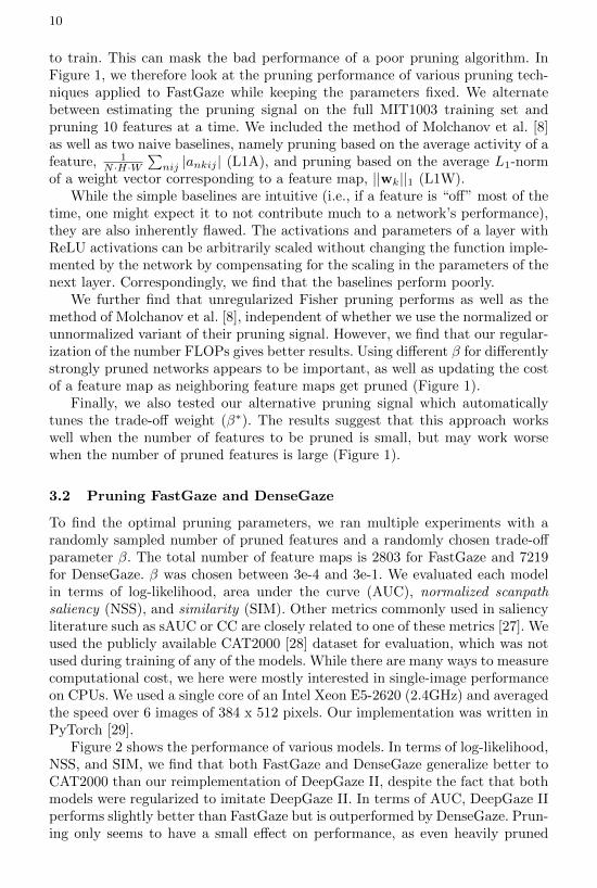
Fig. 1. Comparison of different pruning methods applied to FastGaze withoutretraining. We compared Fisher pruning to two baselines and the method ofMolchanov et al. [8]. For the latter, we ran the normalized/unnormalized and regu-larized/unregularized variants (gray lines). This plot shows that naive methods do notwork well (green lines), that using different regularization weights is important, andthat updating estimates of the computational cost during pruning is important foroptimal performance (orange lines).

Our saliency models were trained in several steps. First, we trained a DeepGaze IImodel using Adam [14] with a batch size of 8 and an initial learning rate of 0.001which was slowly decreased over the course of training. As in [6], the modelwas first pre-trained using the SALICON dataset [15] while using the MIT1003dataset [16] for validation. The validation data was evaluated every 100 stepsand training was stopped when the cross-entropy on the validation data did notdecrease 20 times in a row. The parameters with the best validation score ob-served until then were saved. Afterwards, the MIT1003 dataset was split into 10training and validation sets and used to train 10 DeepGaze II models again withearly stopping.

The ensemble of DeepGaze II models was used to generate an average saliencymap for each image in the SALICON dataset. These saliency maps were thenused for knowledge distillation [7]. This additional data allows us to not onlytrain the readout network of our own models, but also fine-tune the underlyingfeature representation. We used a weighted combination of the cross-entropy for

7

MIT1003 and the cross-entropy with respect to the DeepGaze II saliency maps,using weights of 0.1 and 0.9, respectively.

After training our models to convergence, we start pruning the network. Weaccumulated pruning signals (Equation 7) for 10 training steps while continuingto update the parameters before pruning a single feature map. The feature mapwas selected to maximize the reduction in the combined cost (Equation 13). Wetried to apply early stopping to the combined cost to automatically determinean appropriate number of feature maps to prune, however, we found that earlystopping terminated too early and we therefore opted to treat the number ofpruned features as another hyperparameter which we optimized via randomsearch. During the pruning phase we used SGD with a fixed learning rate of0.0025 and momentum of 0.9, as we found that this led to slightly better resultsthan using Adam. This may be explained by a regularizing effect of SGD [17].

2.5 Related Work

Many recent papers have used pretrained neural networks as feature extractorsfor the prediction of fixations [5,18,6,19,20]. Most closely related to our work isthe DeepGaze approach [5,6]. In contrast to DeepGaze, here we also finetune thefeature representations, which despite the limited amount of available fixationdata is possible because we use a combination of knowledge distillation andpruning to regularize our networks. Kruthiventi et al. [18] also tried to finetunea pretrained network by using a smaller learning rate for pretrained parametersthan for other parameters. Vig et al. [21] trained a smaller network end-to-end but did not start from a pretrained representation and therefore did notachieve the performance of current state-of-the-art architectures. Similarly, Panet al. [22] trained networks end-to-end while initializing only a few layers withparameters obtained from pretrained networks but have since been outperformedby DeepGaze II and other recent approaches.

To our knowledge, none of this prior work has addressed the question of howmuch computation is actually needed to achieve good performance.

Many heuristics have been developed for pruning [23,24,8]. More closely re-lated to ours are methods which try to directly estimate the effect on the loss.Optimal brain damage [12], for example, starts from a 2nd order approximationof a squared error loss and computes second derivatives analytically by perform-ing an additional backward pass. Optimal brain surgeon [13] extends this methodand automatically tries to correct parameters after pruning by computing thefull Hessian. In contrast, our pruning signal only requires gradient informationwhich is already computed during the backward pass. This makes the proposedFisher pruning not only more efficient but also easier to implement.

Most closely related to our pruning method is the approach of Molchanovet al. [8]. By combining a 1st order approximation with heuristics, they arriveat a very similar estimate of the change in loss due to pruning. We found thatin practice, both estimates performed similarly when used without regulariza-tion (Figure 1). The main contribution in Section 2.1 is a new derivation whichprovides a more principled motivation for the pruning signal.

8

Table 1. Comparison of pruning methods for the LeNet-5 network trained onMNIST [26]

Method Error Computational cost

LeCun et al. [26] 0.80% 100%Han et al. [24] 0.77% 16%Fisher (β = 0) 0.84% 26%Fisher (β > 0) 0.79% 10%Fisher (β∗) 0.86% 17%

Unlike most papers on pruning, Molchanov et al. [8] also explicitly regular-ized the computational complexity of the network. However, their approach toregularization differs from ours in two ways. First, a fixed weight was used forthe computational cost while pruning a different number of feature maps. Incontrast, here we recognize that each setting of β creates a separate optimiza-tion problem with its own optimal architecture. In practice, we find that thespeed and architecture of a network is heavily influenced by the choice of β evenwhen pruning the same number of feature maps, suggesting that using differentweights is important. Molchanov et al. [8] further only estimated the compu-tational cost of each feature map once before starting to prune. This leads tosuboptimal pruning, as the computational cost of a feature map changes whenneighboring layers are pruned (Figure 1).

3 Experiments

In the following, we first validate the performance of Fisher pruning on a simplertoy example. We then explore the performance and computational cost of twoarchitectures for saliency prediction. First, we try using the smaller VGG-11variant of Simonyan et al. [9] for feature extraction. In contrast to the readoutnetwork of Kummerer et al. [6], which took as input feature maps from 5 differentlayers, we only used the output of the last convolutional layer (“conv5 2”) asinput. Extracting information from multiple layers is less important in our case,since we are also optimizing the parameters of the feature extraction network.As an alternative to VGG, we try DenseNet-121 as a feature extractor [11], usingthe output of “dense block 3” as input to the readout network. In both cases,the readout network consisted of convolutions with parametric rectified linearunits [25] and 32, 16, and 2 feature maps in the hidden layers. In the following,we will call the first network FastGaze and the second network DenseGaze.

3.1 Fisher Pruning

We apply Fisher pruning to the example of a LeNet-5 network trained on theMNIST dataset [26]. We compare our method to the pruning method of Han etal. [24] which requires L1 or L2 regularization of the model’s parameters duringan initial training phase and cannot directly be applied to a pretrained model.

9

62 125 250 500 1000 2000 4000Speed [ms]

13.60

13.56

13.52

13.48

13.44

13.40Log-likelihood [nat]

62 125 250 500 1000 2000 4000Speed [ms]

0.610.620.630.640.650.660.670.680.69

SIM

62 125 250 500 1000 2000 4000Speed [ms]

0.850

0.855

0.860

0.865

0.870

0.875

0.880AUC

62 125 250 500 1000 2000 4000Speed [ms]

1.8

1.9

2.0

2.1

2.2

2.3NSS

Fig. 2. Speed and performance of various models trained on MIT1003 and evaluatedon the CAT2000 training set. Each point corresponds to a different architecture with adifferent number of pruned features and a different β. Solid lines mark Pareto optimalmodels. In some cases, only a single model is Pareto optimal and no solid line is shown.The x-axis shows speed measured on a CPU for a single image as input. FastGazereaches faster speeds than DenseGaze, especially when explicitly optimized to reducethe amount of floating point operations (β > 0). With the exception of SIM, DenseGazereaches higher prediction performance. For all metrics, even heavily pruned modelsappear to generalize as well or better to CAT2000 than DeepGaze II.

LeNet-5 consists of two convolutional layers and two pooling layers, followed bytwo fully connected layers. Following Han et al. [24], the details of the initialarchitecture were the same as in the MNIST example provided by the Caffeframework 1. We used 53000 data points of the training set for training and7000 data points for validation and early stopping.

We find that Fisher pruning performs well, but that taking the computationalcost into account is important (Table 1). Automatically choosing the weightcontrolling the trade-off between performance and computational cost worksbetter than ignoring computational cost (β∗), although not as well as using afixed but optimized weight (β > 0).

An incorrect decision of a pruning algorithm may be corrected by retrainingthe network’s weights, especially for toy examples like LeNet-5 which are quick

1 https://github.com/BVLC/caffe/

10

to train. This can mask the bad performance of a poor pruning algorithm. InFigure 1, we therefore look at the pruning performance of various pruning tech-niques applied to FastGaze while keeping the parameters fixed. We alternatebetween estimating the pruning signal on the full MIT1003 training set andpruning 10 features at a time. We included the method of Molchanov et al. [8]as well as two naive baselines, namely pruning based on the average activity of afeature, 1

N ·H·W∑nij |ankij | (L1A), and pruning based on the average L1-norm

of a weight vector corresponding to a feature map, ||wk||1 (L1W).While the simple baselines are intuitive (i.e., if a feature is “off” most of the

time, one might expect it to not contribute much to a network’s performance),they are also inherently flawed. The activations and parameters of a layer withReLU activations can be arbitrarily scaled without changing the function imple-mented by the network by compensating for the scaling in the parameters of thenext layer. Correspondingly, we find that the baselines perform poorly.

We further find that unregularized Fisher pruning performs as well as themethod of Molchanov et al. [8], independent of whether we use the normalized orunnormalized variant of their pruning signal. However, we find that our regular-ization of the number FLOPs gives better results. Using different β for differentlystrongly pruned networks appears to be important, as well as updating the costof a feature map as neighboring feature maps get pruned (Figure 1).

Finally, we also tested our alternative pruning signal which automaticallytunes the trade-off weight (β∗). The results suggest that this approach workswell when the number of features to be pruned is small, but may work worsewhen the number of pruned features is large (Figure 1).

3.2 Pruning FastGaze and DenseGaze

To find the optimal pruning parameters, we ran multiple experiments with arandomly sampled number of pruned features and a randomly chosen trade-offparameter β. The total number of feature maps is 2803 for FastGaze and 7219for DenseGaze. β was chosen between 3e-4 and 3e-1. We evaluated each modelin terms of log-likelihood, area under the curve (AUC), normalized scanpathsaliency (NSS), and similarity (SIM). Other metrics commonly used in saliencyliterature such as sAUC or CC are closely related to one of these metrics [27]. Weused the publicly available CAT2000 [28] dataset for evaluation, which was notused during training of any of the models. While there are many ways to measurecomputational cost, we here were mostly interested in single-image performanceon CPUs. We used a single core of an Intel Xeon E5-2620 (2.4GHz) and averagedthe speed over 6 images of 384 x 512 pixels. Our implementation was written inPyTorch [29].

Figure 2 shows the performance of various models. In terms of log-likelihood,NSS, and SIM, we find that both FastGaze and DenseGaze generalize better toCAT2000 than our reimplementation of DeepGaze II, despite the fact that bothmodels were regularized to imitate DeepGaze II. In terms of AUC, DeepGaze IIperforms slightly better than FastGaze but is outperformed by DenseGaze. Prun-ing only seems to have a small effect on performance, as even heavily pruned

11

Table 2. Comparison of deep models evaluated on the MIT300 benchmark dataset.For reference, we also include the performance of a Gaussian center bias. Results ofcompeting methods were obtained from the benchmark’s website [30]. The last columncontains the computational cost in terms of the number of floating point operationsrequired to process a 640 × 480 pixel input

Model AUC KL SIM NSS GFLOP

Center Bias 78% 1.24 0.45 0.92 -eDN [21] 82% 1.14 0.41 1.14 -SalNet [22] 83% 0.81 0.52 1.51 -DeepGaze I [5] 84% 1.23 0.39 1.22 -SAM-ResNet [31] 87% 1.27 0.68 2.34 -DSCLRCN 87% 0.95 0.68 2.35 -DeepFix [18] 87% 0.63 0.60 2.26 -SALICON [32] 87% 0.54 0.60 2.12 -DeepGaze II [6] 88% 0.96 0.46 1.29 240.6FastGaze 85% 1.21 0.61 2.00 10.7DenseGaze 86% 1.20 0.63 2.16 12.8

models still perform well. For the same AUC, we achieve a speedup of roughly 10xwith DenseGaze, while in terms of log-likelihood even our most heavily prunedmodel yielded better performance (which corresponds to a speedup of morethan 75x). Comparing DenseGaze and FastGaze, we find that while DenseGazeachieves better AUC performance, FastGaze is able to achieve faster runtimesdue to its less complex architecture.

We find that explicitly regularizing computational complexity is important.For the same AUC and depending on the amount of pruning, we observe speedupsof up to 2x for FastGaze when comparing regularized and non-regularized mod-els.

In Figure 3 we visualize some of the pruned FastGaze models. We find that atlower computational complexity, optimal architectures have a tendency to alter-nate between convolutions with large and small numbers of feature maps. Thismakes sense when only considering the computational cost of a convolutionallayer (Equation 11), but it is interesting to see that such an architecture canstill perform well in terms of fixation prediction, which requires the detection ofvarious types of objects.

Qualitative results are provided in Figure 4. Even at large reductions incomputational complexity, the fixation predictions appear very similar. At aspeedup of 39x compared to DeepGaze II, the saliency maps start to become abit blurrier, but generally detect the same structures. In particular, the modelstill responds to faces, people, objects, signs, and text.

To verify that our models indeed perform close to the state of the art, wesubmitted saliency maps to the MIT Saliency Benchmark [30,33,34]. We com-puted saliency maps for the MIT300 test set, which contains 300 more images ofthe same type as MIT1003. We evaluated a FastGaze model which took 356msto evaluate in PyTorch, (2250 pruned features, β = 0.0001) and a DenseGaze

12

model which took 577ms (2701 pruned features, β = 3 ·10−5). We find that bothmodels perform slightly below the state of the art when evaluated on MIT300(Table 2), but are still comparable to other recent deep saliency models. We ex-plain the discrepancy by the fact that the submitted models were chosen for theirperformance on CAT2000. That is, they generalize very well to other datasets,but may have lost information about the subtleties of the MIT datasets.

4 Conclusion

We have described a principled pruning method which only requires gradientsas input, and which is efficient and easy to implement. Unlike most pruningmethods, we explicitly penalized computational complexity and tried to find thearchitecture which optimally optimizes a given trade-off between performanceand computational complexity. With this we were able to show that the computa-tional complexity of state-of-the-art saliency models can be drastically reducedwhile maintaining a similar level of performance. Together with a knowledgedistillation approach, the reduced complexity allowed us to train the modelsend-to-end and achieve good generalization performance.

In settings where training is expensive, trying out many different parametersto tune the trade-off between computational complexity and performance maynot be feasible. We have discussed an alternative pruning signal which takes intoaccount computational complexity but is free of hyperparameters. This approachdoes not only apply to Fisher pruning, but can be combined with any pruningsignal estimating the importance of a feature map or parameter.

Less resource intensive models are of particular importance in applicationswhere a lot of data is processed, as well as in applications running on resourceconstrained devices such as mobile phones. Faster gaze prediction models alsohave the potential to speed up the development of video models. The largernumber of images to be processed in videos impacts training times, making itmore difficult to iterate models. Another issue is that the amount of fixationtraining data in existence is fairly limited for videos. Smaller models will allowfor faster training times and a more efficient use of the available training data.

13

Fig. 3. The top graph visualizes the feature maps of the unpruned FastGaze model,while the remaining graphs visualize models pruned to different degrees. Labels in-dicate the number of feature maps. From top to bottom, the measured runtime forthese models was 1.39s, 356ms, 258ms, and 91ms. For strongly regularized models, weobserved a tendency to alternate between convolutions with many feature maps andconvolutions with very few feature maps. The top left corner shows an example inputimage and ground truth fixations, while the right column shows saliency models gener-ated by the different models. Despite a 15x difference in speed, the saliency maps arevisually very similar.

14

Data

Dee

pGaze

II(3

.59s)

Den

seGaze

(577m

s)FastGaze

(356m

s)FastGaze

(91m

s)

Fig. 4. Example saliency maps generated for images of the CAT2000 dataset. (Theoriginal images contained gray borders which were cropped in this visualization.) In-tensities correspond to gamma-corrected fixation probabilities, where black and whitecorrespond to the 1% and 99% percentile of saliency values for a given image, respec-tively. Saliency maps in the second row were generated by an ensemble of DeepGaze IImodels, but we report the time for a single model. Rows 3 and 4 show saliency maps ofonly slightly pruned DenseGaze and FastGaze models, while the last row shows saliencymaps of a heavily pruned model. We find all models produce similar saliency maps.In particular, even the heavily pruned model (39x speedup compared to DeepGaze II)still responds to faces, people, other objects, and text.

15

References

1. Ardizzone, E., Bruno, A., Mazzola, G. In: Saliency Based Image Cropping. SpringerBerlin Heidelberg (2013) 773–782

2. Feng, Y., Cheung, G., Tan, W.T., Ji, Y.: Gaze-driven video streaming withsaliency-based dual-stream switching. In: IEEE Visual Communications and ImageProcessing (VCIP). (2012)

3. Xu, P., Sugano, Y., Bulling, A.: Spatio-temporal modeling and prediction of visualattention in graphical user interfaces. In: Proceedings of the 2016 CHI Conferenceon Human Factors in Computing Systems. (2016)

4. Koch, C., Ullman, S.: Shifts in selective visual attention: towards the underlyingneural circuitry. Human Neurobiology 4 (1985) 219–227

5. Kummerer, M., Theis, L., Bethge, M.: Deep Gaze I: Boosting Saliency Predictionwith Feature Maps Trained on ImageNet. In: ICLR Workshop. (May 2015)

6. Kummerer, M., Wallis, T.S.A., Bethge, M.: DeepGaze II: Reading fixations fromdeep features trained on object recognition. ArXiv e-prints (October 2016)

7. Hinton, G., Vinyals, O., Dean, J.: Distilling the Knowledge in a Neural Network.ArXiv e-prints (2015)

8. Molchanov, P., Tyree, S., Karras, T., Aila, T., Kautz, J.: Pruning convolutionalneural networks for resource efficient inference. In: International Conference onLearning Representations (ICLR). (2017)

9. Simonyan, K., Zisserman, A.: Very Deep Convolutional Networks for Large-ScaleImage Recognition. ArXiv e-prints (September 2014)

10. Nair, V., Hinton, G.: Rectified linear units improve restricted boltzmann machines.In: Proceedings of the 27th International Conference on Machine Learning. (2010)

11. Huang, G., Liu, Z., van der Maaten, L., Weinberger, K.Q.: Densely connectedconvolutional networks. In: The IEEE Conference on Computer Vision and PatternRecognition (CVPR). (2017)

12. LeCun, Y., Denker, J.S., Solla, S.A.: Optimal Brain Damage. In Touretzky, D.S.,ed.: Advances in Neural Information Processing Systems 2. Morgan-Kaufmann(1990) 598–605

13. Hassibi, B., Stork, D.G.: Second order derivatives for network pruning: Optimalbrain surgeon. In: Advances in Neural Information Processing Systems. (1993)164–171

14. Kingma, D.P., Ba, J.: Adam: A method for stochastic optimization. In: Proceedingsof the 3rd International Conference on Learning Representations (ICLR). (2015)

15. Jiang, M., Huang, S., Duan, J., Zhao, Q.: SALICON: Saliency in Context. In: TheIEEE Conference on Computer Vision and Pattern Recognition (CVPR). (June2015)

16. Judd, T., Ehinger, K., Durand, F., Torralba, A.: Learning to predict where humanslook. In: IEEE International Conference on Computer Vision (ICCV). (2009)

17. Zhang, C., Bengio, S., Hardt, M., Recht, B., Vinyals, O.: Understanding deep learn-ing requires rethinking generalization. In: International Conference on LearningRepresentations (ICLR). (2017)

18. Kruthiventi, S.S.S., Ayush, K., Babu, R.V.: DeepFix: A Fully Convolutional NeuralNetwork for Predicting Human Eye Fixations. In: IEEE Transactions on ImageProcessing. Volume 26. (2017)

19. Tavakoli, H.R., Borji, A., Laaksonen, J., Rahtu, E.: Exploiting inter-image simi-larity and ensemble of extreme learners for fixation prediction using deep features.Neurocomputing 244(Supplement C) (2017) 10 – 18

16

20. Liu, N., Han, J.: A deep spatial contextual long-term recurrent convolutionalnetwork for saliency detection. CoRR abs/1610.01708 (2016)

21. Vig, E., Dorr, M., Cox, D.: Large-Scale Optimization of Hierarchical Features forSaliency Prediction in Natural Images. In: The IEEE Conference on ComputerVision and Pattern Recognition (CVPR). (2014)

22. Pan, J., Sayrol, E., Giro-i Nieto, X., McGuinness, K., O’Connor, N.E.: Shallowand deep convolutional networks for saliency prediction. In: The IEEE Conferenceon Computer Vision and Pattern Recognition (CVPR). (June 2016)

23. Li, H., Kadav, A., Durdanovic, I., Samet, H., Graf, H.P.: Pruning filters for efficientconvnets. In: International Conference on Learning Representations (ICLR). (2017)

24. Han, S., Pool, J., Tran, J., Dally, W.J.: Learning both weights and connections forefficient neural networks. In: Advances in Neural Information Processing Systems.(2015)

25. He, K., Zhang, X., Ren, S., , Sun, J.: Delving Deep into Rectifiers: SurpassingHuman-Level Performance on ImageNet Classification. In: IEEE InternationalConference on Computer Vision (ICCV). (2015)

26. LeCun, Y., Bottou, L., Bengio, Y., Haffner, P.: Gradient-based learning applied todocument recognition. In: Proceedings of the IEEE. Volume 86. (1998) 2278–2324

27. Kmmerer, M., Wallis, T.S.A., Bethge, M.: Saliency benchmarking: Separatingmodels, maps and metrics. arxiv (Apr 2017)

28. Borji, A., Itti, L.: CAT2000: A Large Scale Fixation Dataset for Boosting SaliencyResearch. CVPR 2015 workshop on ”Future of Datasets” (2015) arXiv preprintarXiv:1505.03581.

29. PyTorch. https://github.com/pytorch

30. Bylinskii, Z., Judd, T., Borji, A., Itti, L., Durand, F., Oliva, A., Torralba, A.: MITSaliency Benchmark

31. Cornia, M., Baraldi, L., Serra, G., Cucchiara, R.: Predicting human eye fixationsvia an lstm-based saliency attentive model. CoRR abs/1611.09571 (2016)

32. Huang, X., Shen, C., Boix, X., Zhao, Q.: SALICON: Reducing the semantic gap insaliency prediction by adapting deep neural networks. In: The IEEE InternationalConference on Computer Vision (ICCV). (2015)

33. Judd, T., Durand, F., Torralba, A.: A benchmark of computational models ofsaliency to predict human fixations. Technical report, MIT technical report (2012)

34. Bylinskii, Z., Judd, T., Oliva, A., Torralba, A., Durand, F.: What do differentevaluation metrics tell us about saliency models? CoRR abs/1604.03605 (2016)

17

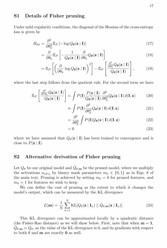
S1 Details of Fisher pruning

Under mild regularity conditions, the diagonal of the Hessian of the cross-entropyloss is given by

Hkk =∂2

∂θ2kEP [− logQθ(z | I)] (17)

=∂

∂θkEP[− 1

Qθ(z | I)∂

∂θkQθ(z | I)

](18)

= EP

[(∂

∂θklogQθ(z | I)

)2]− EP

∂2

∂θ2kQθ(z | I)

Qθ(z | I)

, (19)

where the last step follows from the quotient rule. For the second term we have

EP

[∂2

∂2θkQθ(z | I)

Qθ(z | I)

]=

∫P (I)

P (z | I)Qθ(z | I)

∂2

∂θ2kQθ(z | I) d(I, z) (20)

≈∫P (I)

∂2

∂θ2kQθ(z | I) d(I, z) (21)

=∂2

∂θ2k

∫P (I)Qθ(z | I) d(I, z) (22)

= 0 (23)

where we have assumed that Qθ(z | I) has been trained to convergence and isclose to P (z | I).

S2 Alternative derivation of Fisher pruning

Let Qθ be our original model and Qθ,m be the pruned model, where we multiplythe activations ankij by binary mask parameters mk ∈ {0, 1} as in Eqn. 8 ofthe main text. Pruning is achieved by setting mk = 0 for pruned features, andmk = 1 for features we wish to keep.

We can define the cost of pruning as the extent to which it changes themodel’s output, which can be measured by the KL divergence

L(m) =1

N

N∑n=1

KL[Qθ(z | In) || Qθ,m(z | In)]. (24)

This KL divergence can be approximated locally by a quadratic distance(the Fisher-Rao distance) as we will show below. First, note that when m = 1,Qθ,m ≡ Qθ, so the value of the KL divergence is 0, and its gradients with respectto both θ and m are exactly 0 as well.

18

Thus, we can approximate L by its second-order Taylor-approximation aroundthe unpruned model m = 1 as follows:

L(m) ≈ 1

2(m− 1)>H(m− 1), (25)

where H = ∇2L(1) is the Hessian of L at m = 1.Pruning a single feature k amounts to setting mk = 1− ek, where ek is the

unit vector which is zero everywhere except at its ith entry, where it is 1. Thecost of pruning a single feature k is then approximated as:

`k = L(1− ek) ≈ 1

2Hkk (26)

Under some mild conditions, the Hessian of L at m = 1 is the Fisher infor-mation matrix, which can be approximated by the empirical Fisher information.In particular for the diagonal terms Hkk we have that:

1

2Hkk = − ∂2

∂m2k

1

2N

N∑n=1

EQθ,1[log Qθ,1(z | In)

](27)

=1

2N

N∑n=1

EQθ,1

[(∂

∂mklog Qθ,1(z | In)

)2]

(28)

=1

2N

N∑n=1

EQθ

[(an,i,j,k

∂

∂an,i,j,klog Qθ,1(z | In)

)2]

(29)

=1

2N

N∑n=1

a2n,i,j,kEQθ

[(∂

∂an,i,j,klogQθ(z | In)

)2]

(30)

≈ 1

2N

N∑n=1

a2n,i,j,k

(∂

∂an,i,j,klogQθ(zn | In)

)2

(31)

=1

2N

N∑n=1

g2nk, (32)

where gnk is defined as in Eqn. 9 of the main text.