Fast Perceptron Decision Tree Learning fromEvolving Data Streams

Albert Bifet, Geoff Holmes, Bernhard Pfahringer, and Eibe Frank

University of Waikato, Hamilton, New Zealand{abifet,geoff,bernhard,eibe}@cs.waikato.ac.nz

Abstract. Mining of data streams must balance three evaluation dimen-sions: accuracy, time and memory. Excellent accuracy on data streamshas been obtained with Naive Bayes Hoeffding Trees—Hoeffding Treeswith naive Bayes models at the leaf nodes—albeit with increased run-time compared to standard Hoeffding Trees. In this paper, we showthat runtime can be reduced by replacing naive Bayes with perceptronclassifiers, while maintaining highly competitive accuracy. We also showthat accuracy can be increased even further by combining majority vote,naive Bayes, and perceptrons. We evaluate four perceptron-based learn-ing strategies and compare them against appropriate baselines: simpleperceptrons, Perceptron Hoeffding Trees, hybrid Naive Bayes PerceptronTrees, and bagged versions thereof. We implement a perceptron that usesthe sigmoid activation function instead of the threshold activation func-tion and optimizes the squared error, with one perceptron per class value.We test our methods by performing an evaluation study on synthetic andreal-world datasets comprising up to ten million examples.

1 Introduction

In the data stream model, data arrive at high speed, and algorithms that processthem must do so under very strict constraints of space and time. Consequently,data streams pose several challenges for data mining algorithm design. First,algorithms must make use of limited resources (time and memory). Second, theymust deal with data whose nature or distribution changes over time.

An important issue in data stream mining is the cost of performing thelearning and prediction process. As an example, it is possible to buy time andspace usage from cloud computing providers [25]. Several rental cost optionsexist:

– Cost per hour of usage: Amazon Elastic Compute Cloud (Amazon EC2) isa web service that provides resizable compute capacity in the cloud. Costdepends on the time and on the machine rented (small instance with 1.7 GB,large with 7.5 GB or extra large with 15 GB).

– Cost per hour and memory used: GoGrid is a web service similar to AmazonEC2, but it charges by RAM-Hours. Every GB of RAM deployed for 1 hourequals one RAM-Hour.

It is crucial to find mining methods that use resources efficiently. In this spirit, wepropose in this paper the Hoeffding Perceptron Tree for classification, as a fastermethod compared to the state-of-the-art Hoeffding Tree with naive Bayes leaves.The idea is to implement perceptron classifiers at the leaves of the HoeffdingTree, to potentially increase accuracy, but mainly to reduce runtime.

We introduce the use of RAM-Hours as an evaluation measure of the re-sources used by streaming algorithms. The paper is structured as follows: relatedwork is presented in Section 2. Hoeffding Perceptron Trees and bagging of suchtrees are discussed in Section 3. An experimental evaluation is conducted in Sec-tion 4. Finally, conclusions and suggested items for future work are presented inSection 5.

2 Related Work

Standard decision tree learners such as ID3, C4.5, and CART [18, 21] assumethat all training examples can be stored simultaneously in main memory, andare thus severely limited in the number of examples they can learn from. Inparticular, they are not applicable to data streams, where potentially there isno bound on the number of examples and these arrive sequentially.

Domingos et al. [6, 14] proposed the Hoeffding tree as an incremental, anytimedecision tree induction algorithm that is capable of learning from data streams,assuming that the distribution generating examples does not change over time.

Hoeffding trees exploit the fact that a small sample can often suffice to choosea splitting attribute. This idea is supported by the Hoeffding bound, whichquantifies the number of observations (in our case, examples) needed to estimatesome statistics within a prescribed precision (in our case, the goodness of anattribute). More precisely, the Hoeffding bound states that with probability 1−δ,the true mean of a random variable of range R will not differ from the estimatedmean after n independent observations by more than:

ε =

√R2 ln(1/δ)

2n.

A theoretically appealing feature of Hoeffding Trees not shared by other incre-mental decision tree learners (ID4 [22], ID5 [24]) is that it has sound guaranteesof performance. Using the Hoeffding bound one can show that its output isasymptotically nearly identical to that of a non-incremental learner using in-finitely many examples. CVFDT [14] is an extension of the Hoeffding Tree toevolving data streams, but does not exhibit theoretical guarantees.

Outside the data stream world, there is prior work on using perceptrons orsimilar classifiers in decision trees. Utgoff [24] presented the Perceptron DecisionTree as a decision tree in which each leaf node uses the perceptron as a classifierof the input instances. Bennett et al. [2] showed that maximizing margins inperceptron decision trees can be useful to combat overfitting. Zhou [26] proposedHybrid Decision Trees as a hybrid learning approach combining decision treeswith neural networks.

Frank et al. [7] investigated using Model Trees for classification problems.Model trees are decision trees with linear regression functions at the leaves.Logistic Model Trees [17] are model trees that use logistic regression insteadof linear regression. They have been shown to be very accurate and compactclassifiers, but their induction is very time-consuming.

The LTree algorithm of Gama [8] embodies a general framework for learn-ing functional trees, multivariate classification or regression trees that can usecombinations of attributes at decision nodes, leaf nodes, or both.

In the data streams literature, Ikonomovska et al. [15] presented FIMT, afast incremental model tree for regression on static data streams. To deal withconcept drift, Ikonomovska et al. [16] proposed FIRT-DD as an adaption ofthe FIMT algorithm to time-changing distributions. FIMT and FIRT-DD use aperceptron learner at the leaves to perform regression. Considering classificationmethods for data streams, Bifet et al. [4] presented two new ensemble learningmethods: one using bagging with decision trees of different size and one usingADWIN, an adaptive sliding window method that detects change and adjusts thesize of the window correspondingly. We revisit the latter approach in this paper.

3 Perceptrons and Hoeffding Perceptron Trees

In this section, we present the perceptron learner we use, and the Hoeffding Per-ceptron Tree based on it. We also consider bagging trees with change detection.

3.1 Perceptron Learning

We use an online version of the perceptron that employs the sigmoid activationfunction instead of the threshold activation function and optimizes the squarederror, with one perceptron per class value.

Given a data stream 〈xi, yi〉, where xi is an example and yi is its exampleclass, the classifier’s goal is to minimize the number of misclassified examples.Let hw(xi) be the hypothesis function of the perceptron for instance xi. Weuse the mean-square error J(w) = 1

2

∑(yi − hw(xi))

2 instead of the 0-1 lossfunction, since it is differentiable.

The classic perceptron takes a linear combination and thresholds it. Thepredicted class of the perceptron is hw(xi) = sgn(wTxi), where a bias weightwith constant input is included. Our hypothesis function hw = σ(wTx) insteaduses the sigmoid function σ(x) = 1/(1 + e−x) since it has the property σ′(x) =σ(x)(1− σ(x)). Thus, we can compute the gradient of the error function

∇J = −∑i

(yi − hw(xi))∇hw(xi)

where for sigmoid hypothesis

∇hw(xi) = hw(xi)(1− hw(xi))

obtaining the following weight update rule

w = w + η∑i

(yi − hw(xi))hw(xi)(1− hw(xi))xi

Because we work in a data stream scenario, rather than performing batchupdates, we use stochastic gradient descent where the weight vector is updatedafter every example. As we deal with multi-class problems, we train one per-ceptron for each class. To classify an unseen instance x, we obtain the pre-dictions hw1(x), . . . , hwn(x) from the perceptrons, and the predicted class isarg maxclass hwclass(x). The pseudocode is shown in Figure 1.

Perceptron Learning(Stream, η)

1 for each class2 do Perceptron Learning(Stream, class, η)

Perceptron Learning(Stream, class, η)

1 � Let w0 and w be randomly initialized2 for each example (x, y) in Stream3 do if class = y4 then δ = (1− hw(x)) · hw(x) · (1− hw(x))5 else δ = (0− hw(x)) · hw(x) · (1− hw(x))6 w = w + η · δ · x

Perceptron Prediction(x)

1 return arg maxclass hwclass(x)

Fig. 1. Perceptron algorithm

3.2 Hoeffding Perceptron Tree

Hoeffding trees [6] are state-of-the-art in classification for data streams and theyperform prediction by choosing the majority class at each leaf. Their predictiveaccuracy can be increased by adding naive Bayes models at the leaves of the trees.However, Holmes et al. [12] identified situations where the naive Bayes methodoutperforms the standard Hoeffding tree initially but is eventually overtaken.They propose a hybrid adaptive method that generally outperforms the twooriginal prediction methods for both simple and complex concepts. We call thismethod Hoeffding Naive Bayes Tree (hnbt). This method works by performinga naive Bayes prediction per training instance, and comparing its predictionwith the majority class. Counts are stored to measure how many times the naiveBayes prediction gets the true class correct as compared to the majority class.

When performing a prediction on a test instance, the leaf will only return a naiveBayes prediction if it has been more accurate overall than the majority class,otherwise it resorts to a majority class prediction.

We adapt this methodology to deal with perceptrons rather than naive Bayesmodels. A Hoeffding Perceptron Tree (hpt) is a Hoeffding Tree that has a per-ceptron at each leaf. Similarly to hnbt, predictions by the perceptron are onlyused if they are more accurate on average than the majority class. It improveson hnbt in terms of runtime because it does not need to estimate the statisticaldistribution for numeric attributes and calculate density values based on theexponential function, and for discrete attributes it does not need to calculatedivisions to estimate probabilities.

Finally, a Hoeffding Naive Bayes Perceptron Tree (hnbpt) is a HoeffdingTree that has three classifiers at each leaf: a majority class, naive Bayes, and aperceptron. Voting is used for prediction. It is slower than the Hoeffding Percep-tron Tree and the Hoeffding Naive Bayes Tree, but it combines the predictivepower of the base learners.

3.3 Bagging Trees with ADWIN

ADWIN [3] is a change detector and estimator that solves in a well-specified waythe problem of tracking the average of a stream of bits or real-valued numbers.ADWIN keeps a variable-length window of recently seen items, with the prop-erty that the window has the maximal length statistically consistent with thehypothesis “there has been no change in the average value inside the window”.

ADWIN is parameter- and assumption-free in the sense that it automaticallydetects and adapts to the current rate of change. Its only parameter is a confi-dence bound δ, indicating how confident we want to be in the algorithm’s output,inherent to all algorithms dealing with random processes.

Also important for our purposes, ADWIN does not maintain the window ex-plicitly, but compresses it using a variant of the exponential histogram technique.This means that it keeps a window of length W using only O(logW ) memoryand O(logW ) processing time per item.

ADWIN Bagging is the online bagging method of Oza and Russell [19] withthe addition of the ADWIN algorithm as a change detector. When a change isdetected, the worst classifier of the ensemble of classifiers is removed and a newclassifier is added to the ensemble.

4 Comparative Experimental Evaluation

Massive Online Analysis (MOA) [13] is a software environment for implementingalgorithms and running experiments for online learning from data streams. Allalgorithms evaluated in this paper were implemented in the Java programminglanguage by extending the MOA software.

We use the experimental framework for concept drift presented in [4]. Con-sidering data streams as data generated from pure distributions, we can model

a concept drift event as a weighted combination of two pure distributions thatcharacterizes the target concepts before and after the drift. This framework de-fines the probability that a new instance of the stream belongs to the new conceptafter the drift based on the sigmoid function.

Definition 1. Given two data streams a, b, we define c = a ⊕Wt0 b as the data

stream built by joining the two data streams a and b, where t0 is the point ofchange, W is the length of change, Pr[c(t) = b(t)] = 1/(1 + e−4(t−t0)/W ) andPr[c(t) = a(t)] = 1− Pr[c(t) = b(t)].

In order to create a data stream with multiple concept changes, we can buildnew data streams joining different concept drifts, i. e. (((a⊕W0

t0 b)⊕W1t1 c)⊕W2

t2 d) . . ..

4.1 Datasets for concept drift

Synthetic data has several advantages – it is easier to reproduce and there islittle cost in terms of storage and transmission. For this paper we use the datagenerators most commonly found in the literature.

SEA Concepts Generator This artificial dataset contains abrupt concept drift,first introduced in [23]. It is generated using three attributes, where only thetwo first attributes are relevant. All the attributes have values between 0and 10. The points of the dataset are divided into 4 blocks with differentconcepts. In each block, the classification is done using f1 +f2 ≤ θ, where f1

and f2 represent the first two attributes and θ is a threshold value. The mostfrequent values are 9, 8, 7 and 9.5 for the data blocks. In our framework,SEA concepts are defined as follows:

(((SEA9 ⊕Wt0 SEA8)⊕W

2t0 SEA7)⊕W3t0 SEA9.5)

Rotating Hyperplane This data was used as a testbed for CVFDT versusVFDT in [14]. Examples for which

∑di=1 wixi ≥ w0 are labeled positive,

and examples for which∑d

i=1 wixi < w0 are labeled negative. Hyperplanesare useful for simulating time-changing concepts, because we can change theorientation and position of the hyperplane in a smooth manner by changingthe relative size of the weights.

Random RBF Generator This generator was devised to offer an alternatecomplex concept type that is not straightforward to approximate with adecision tree model. The RBF (Radial Basis Function) generator works asfollows: A fixed number of random centroids are generated. Each center hasa random position, a single standard deviation, class label and weight. Newexamples are generated by selecting a center at random, taking weights intoconsideration so that centers with higher weight are more likely to be chosen.A random direction is chosen to offset the attribute values from the centralpoint. Drift is introduced by moving the centroids with constant speed.

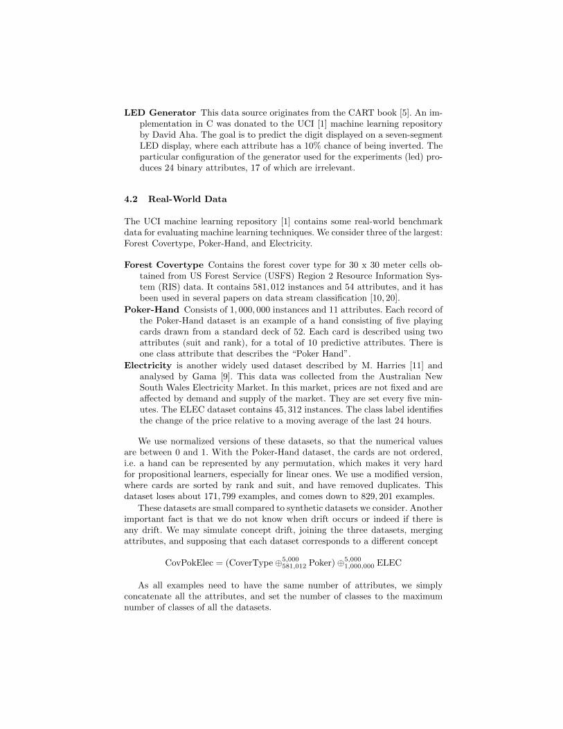
LED Generator This data source originates from the CART book [5]. An im-plementation in C was donated to the UCI [1] machine learning repositoryby David Aha. The goal is to predict the digit displayed on a seven-segmentLED display, where each attribute has a 10% chance of being inverted. Theparticular configuration of the generator used for the experiments (led) pro-duces 24 binary attributes, 17 of which are irrelevant.

4.2 Real-World Data

The UCI machine learning repository [1] contains some real-world benchmarkdata for evaluating machine learning techniques. We consider three of the largest:Forest Covertype, Poker-Hand, and Electricity.

Forest Covertype Contains the forest cover type for 30 x 30 meter cells ob-tained from US Forest Service (USFS) Region 2 Resource Information Sys-tem (RIS) data. It contains 581, 012 instances and 54 attributes, and it hasbeen used in several papers on data stream classification [10, 20].

Poker-Hand Consists of 1, 000, 000 instances and 11 attributes. Each record ofthe Poker-Hand dataset is an example of a hand consisting of five playingcards drawn from a standard deck of 52. Each card is described using twoattributes (suit and rank), for a total of 10 predictive attributes. There isone class attribute that describes the “Poker Hand”.

Electricity is another widely used dataset described by M. Harries [11] andanalysed by Gama [9]. This data was collected from the Australian NewSouth Wales Electricity Market. In this market, prices are not fixed and areaffected by demand and supply of the market. They are set every five min-utes. The ELEC dataset contains 45, 312 instances. The class label identifiesthe change of the price relative to a moving average of the last 24 hours.

We use normalized versions of these datasets, so that the numerical valuesare between 0 and 1. With the Poker-Hand dataset, the cards are not ordered,i.e. a hand can be represented by any permutation, which makes it very hardfor propositional learners, especially for linear ones. We use a modified version,where cards are sorted by rank and suit, and have removed duplicates. Thisdataset loses about 171, 799 examples, and comes down to 829, 201 examples.

These datasets are small compared to synthetic datasets we consider. Anotherimportant fact is that we do not know when drift occurs or indeed if there isany drift. We may simulate concept drift, joining the three datasets, mergingattributes, and supposing that each dataset corresponds to a different concept

CovPokElec = (CoverType⊕5,000581,012 Poker)⊕5,000

1,000,000 ELEC

As all examples need to have the same number of attributes, we simplyconcatenate all the attributes, and set the number of classes to the maximumnumber of classes of all the datasets.

Accuracy

40

45

50

55

60

65

70

75

80

10.000 120.000 230.000 340.000 450.000 560.000 670.000 780.000 890.000 1.000.0

Instances

Ac

cu

rac

y (

%)

htnbp

htnb

htp

ht

Memory

0

0,5

1

1,5

2

2,5

3

3,5

4

4,5

5

10.000 130.000 250.000 370.000 490.000 610.000 730.000 850.000 970.000

Instances

Me

mo

ry (

Mb

)

htnbp

htnb

htp

ht

RunTime

0

5

10

15

20

25

30

35

10.000 120.000 230.000 340.000 450.000 560.000 670.000 780.000 890.000

Instances

Tim

e (

se

c.) htnbp

htnb

htp

ht

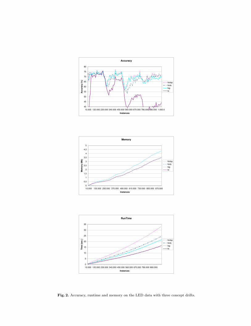
Fig. 2. Accuracy, runtime and memory on the LED data with three concept drifts.

Perceptron Naive Bayes Hoeffding TreeTime Acc. Mem. Time Acc. Mem. Time Acc. Mem.

RBF(0,0) 1.83 72.69± 0.28 0.01 4.15 72.04± 0.06 0.01 5.84 86.75± 0.83 1.56RBF(50,0.001) 2.67 65.33± 0.04 0.01 5.02 53.23± 0.05 0.01 6.40 52.52± 0.17 1.50RBF(10,0.001) 1.82 74.11± 0.09 0.01 4.14 75.79± 0.06 0.01 5.80 83.72± 0.58 1.55RBF(50,0.0001) 2.64 69.34± 0.07 0.01 4.99 53.82± 0.04 0.01 7.04 55.78± 0.33 1.86RBF(10,0.0001) 1.85 73.92± 0.16 0.01 4.14 75.18± 0.09 0.01 5.94 83.59 ± 0.50 1.62HYP(10,0.001) 1.55 92.87± 0.43 0.01 3.91 77.64± 3.74 0.01 5.37 73.19± 2.60 1.60HYP(10,0.0001) 1.56 93.70± 0.03 0.01 3.90 90.23± 0.76 0.01 4.99 76.87± 1.46 1.40SEA(50) 1.17 87.15± 0.05 0.00 1.54 85.37± 0.00 0.00 2.54 85.68± 0.00 0.56SEA(50000) 1.31 86.85± 0.04 0.00 1.69 85.38± 0.00 0.00 2.71 85.59± 0.04 0.56LED(50000) 6.64 72.76± 0.01 0.02 8.97 54.02± 0.00 0.04 12.81 52.74± 0.15 4.98CovType 12.21 81.68 0.05 22.81 60.52 0.08 13.43 68.30 2.59Poker 5.36 3.34 0.01 9.25 59.55 0.02 5.46 73.62 1.11Electricity 0.53 79.07 0.01 0.55 73.36 0.01 0.86 75.35 0.12CovPokElec 20.87 13.69 0.06 56.52 24.34 0.11 42.82 72.63 10.03

69.04 Acc. 67.18 Acc. 73.31 Acc.0.12 RAM-Hours 0.41 RAM-Hours 37 RAM-Hours

Table 1. Comparison of Perceptron, Naive Bayes and Hoeffding Tree. The best indi-vidual accuracies are indicated in boldface.

4.3 Results

We use the datasets explained in the previous sections for evaluation. The exper-iments were performed on a 3 GHz Intel 64-bit machine with 2 GB of memory.The evaluation methodology used was Interleaved Test-Then-Train on 10 runs:every example was used for testing the model before using it to train. This inter-leaved test followed by train procedure was carried out on 10 million examplesfrom the hyperplane and RandomRBF datasets, and one million examples fromthe SEA dataset. The parameters of these streams are the following:

– RBF(x,v): RandomRBF data stream with x centroids moving at speed v.– HYP(x,v): Hyperplane data stream with x attributes changing at speed v.– SEA(v): SEA dataset, with length of change v.– LED(v): LED dataset, with length of change v.

Tables 1, 2 and 3 report the final accuracy, and speed of the classificationmodels induced on the synthetic data and the real datasets: Forest Cover-Type, Poker Hand, Electricity and CovPokElec. Accuracy is measuredas the final percentage of examples correctly classified over the test/train inter-leaved evaluation. Time is measured in seconds, and memory in MB. The classifi-cation methods used are the following: perceptron, naive Bayes, Hoeffding NaiveBayes Tree (hnbt), Hoeffding Perceptron Tree (hpt), Hoeffding Naive BayesPerceptron Tree (hnbpt), and ADWIN bagging using hnbt, hpt, and hnbpt.

The learning curves and model growth curves for the Led dataset are plottedin Figure 2. We observe that ht and hpt are the fastest decision trees. As thetrees do not need more space to compute naive Bayes predictions at the leaves,hnbt uses the same memory as ht, and hpnbt uses the same memory as hpt. Onaccuracy, ht is the method that adapts more slowly to change, and during sometime intervals hpt performs better than hnbt, but in other intervals performsworse. hnbpt is always the most or very close to the most accurate method as

hnbt hpt hnbptTime Acc. Mem. Time Acc. Mem. Time Acc. Mem.

RBF(0,0) 9.03 90.78± 0.46 1.57 8.04 90.33± 0.49 2.30 10.77 91.07± 0.44 2.30RBF(50,0.001) 10.98 57.70± 0.22 1.51 8.66 68.95± 0.31 2.20 11.32 68.65± 0.32 2.20RBF(10,0.001) 9.07 87.24± 0.29 1.56 8.03 87.61± 0.36 2.28 10.77 87.98± 0.32 2.28RBF(50,0.0001) 11.62 69.00± 0.46 1.86 9.54 79.91± 0.42 2.72 12.45 79.88± 0.39 2.72RBF(10,0.0001) 9.28 88.47± 0.37 1.63 8.20 89.37± 0.32 2.38 10.98 89.74± 0.33 2.39HYP(10,0.001) 9.73 83.24± 2.29 1.61 7.57 82.74± 1.13 2.34 11.45 84.54± 1.40 2.34HYP(10,0.0001) 9.37 88.42± 0.36 1.40 7.08 82.59± 0.62 2.04 11.30 88.40± 0.36 2.04SEA(50) 3.70 86.63± 0.00 0.57 4.65 86.73± 0.01 1.23 5.49 87.41± 0.01 1.24SEA(50000) 4.51 86.44± 0.03 0.57 4.85 86.41± 0.07 1.23 5.64 87.12± 0.07 1.24LED(50000) 21.28 68.06± 0.10 4.99 18.64 68.87± 0.07 6.00 24.99 70.04± 0.03 6.00CovType 24.73 81.06 2.59 16.53 83.59 3.46 22.16 85.77 3.46Poker 9.81 83.05 1.12 8.40 74.02 1.82 11.40 82.93 1.82Electricity 0.96 80.69 0.12 0.93 84.24 0.21 1.07 84.34 0.21CovPokElec 68.37 83.41 10.05 49.37 73.33 13.53 69.70 83.28 13.53

81.01 Acc. 81.33 Acc. 83.65 Acc.61.58 RAM-Hours 68.56 RAM-Hours 93.84 RAM-Hours

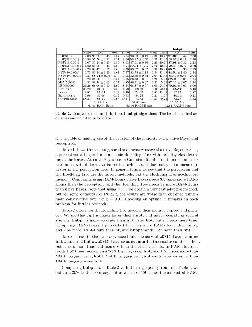
Table 2. Comparison of hnbt, hpt, and hnbpt algorithms. The best individual ac-curacies are indicated in boldface.

it is capable of making use of the decision of the majority class, naive Bayes andperceptron.

Table 1 shows the accuracy, speed and memory usage of a naive Bayes learner,a perceptron with η = 1 and a classic Hoeffding Tree with majority class learn-ing at the leaves. As naive Bayes uses a Gaussian distribution to model numericattributes, with different variances for each class, it does not yield a linear sep-arator as the perceptron does. In general terms, we see that the perceptron andthe Hoeffding Tree are the fastest methods, but the Hoeffding Tree needs morememory. Comparing using RAM-Hours, naive Bayes needs 3.5 times more RAM-Hours than the perceptron, and the Hoeffding Tree needs 89 more RAM-Hoursthan naive Bayes. Note that using η = 1 we obtain a very fast adaptive method,but for some datasets like Poker, the results are worse than obtained using amore conservative rate like η = 0.01. Choosing an optimal η remains an openproblem for further research.

Table 2 shows, for the Hoeffding tree models, their accuracy, speed and mem-ory. We see that hpt is much faster than hnbt, and more accurate in severalstreams. hnbpt is more accurate than hnbt and hpt, but it needs more time.Comparing RAM-Hours, hpt needs 1.11 times more RAM-Hours than hnbt,and 2.54 more RAM-Hours than ht, and hnbpt needs 1.37 more than hpt.

Table 3 reports the accuracy, speed and memory of ADWIN bagging usinghnbt, hpt, and hnbpt. ADWIN bagging using hnbpt is the most accurate method,but it uses more time and memory than the other variants. In RAM-Hours, itneeds 1.62 times more than ADWIN bagging using hpt, and 1.51 times more thanADWIN bagging using hnbt. ADWIN bagging using hpt needs fewer resources thanADWIN bagging using hnbt.

Comparing hnbpt from Table 2 with the single perceptron from Table 1, weobtain a 20% better accuracy, but at a cost of 780 times the amount of RAM-

ADWIN Bagging hnbt ADWIN Bagging hpt ADWIN Bagging hnbptTime Acc. Mem Time Acc. Mem Time Acc. Mem

RBF(0,0) 102.22 94.30± 0.07 16.22 88.84 93.70± 0.10 23.35 115.31 94.36± 0.07 23.98RBF(50,0.001) 88.75 67.67± 0.16 0.12 41.15 74.82± 0.26 2.27 76.34 74.13± 0.40 2.84RBF(10,0.001) 97.65 89.74± 0.09 12.97 80.65 90.36± 0.11 20.44 106.64 90.55± 0.10 19.73RBF(50,0.0001) 90.64 84.99± 0.17 1.33 61.82 87.24± 0.14 9.66 94.22 87.97± 0.11 9.39RBF(10,0.0001) 100.21 91.97± 0.07 13.81 82.54 92.53± 0.12 21.56 109.59 93.01± 0.05 21.32HYP(10,0.001) 90.77 89.92± 0.31 3.02 31.86 91.20± 0.99 1.11 69.23 91.45± 0.81 2.43HYP(10,0.0001) 107.36 91.30± 0.21 8.22 30.77 93.63± 0.21 0.08 50.57 93.61± 0.24 0.11SEA(50) 44.48 88.22± 0.22 4.33 54.09 88.08± 0.07 11.07 59.19 88.60± 0.09 10.17SEA(50000) 41.03 88.61± 0.07 2.69 53.44 87.85± 0.07 10.78 54.07 88.65 ± 0.05 6.83LED(50000) 150.62 73.14± 0.02 5.09 93.09 72.82± 0.03 14.84 130.56 73.02± 0.02 8.45CovType 165.75 85.73 0.80 50.06 86.33 1.66 115.58 87.88 1.25Poker 57.40 74.56 0.09 37.14 65.76 0.21 73.41 74.36 0.16Electricity 3.17 84.36 0.13 2.59 85.22 0.44 3.55 86.44 0.30CovPokElec 363.70 78.96 1.18 118.64 67.02 1.13 402.20 78.77 1.54

84.53 Acc. 84.04 Acc. 85.91 Acc.1028.02 RAM-Hours 957.38 RAM-Hours 1547.33 RAM-Hours

Table 3. Comparison of ADWIN bagging with hnbt, hpt, and hnbpt. The best indi-vidual accuracies are indicated in boldface.

Hours. Comparing ADWIN bagging using hnbpt (Table 3) with a single hnbpt(Table 2) we obtain a 3% better accuracy, at 16.50 times the RAM-Hours.

Concept drift is handled well by the proposed ADWIN bagging algorithms,excluding the poor performance of the hpt-based classifier on CovPokElec,which is due to the nature of the Poker dataset. Decision trees alone do notdeal as well with evolving streaming data, as they have limited capability ofadaption.

A tradeoff between RAM-Hours and accuracy could be to use single per-ceptrons when resources are scarce, and ADWIN bagging methods when moreaccuracy is needed. Note that to gain an increase of 24% in accuracy, we have toincrease by more than 10, 000 times the RAM-Hours needed; this is the differ-ence of magnitude between the RAM-Hours needed for a single perceptron andfor a more accurate ADWIN bagging method.

5 Conclusions

We have investigated four perceptron-based methods for data streams: a singlelearner, a decision tree, a hybrid tree, and an ensemble method. These methodsuse perceptrons with a sigmoid activation function, optimizing the squared error,with one perceptron per class value. We observe that perceptron-based methodsare competitive in accuracy and use of resources. We have introduced the use ofRAM-Hours as a performance measure. Using RAM-Hours, it is easy to compareresources used by classifier algorithms.

As future work, we would like to build new methods based on the perceptron,with an adaptive learning rate. We think that in changing scenarios, using aflexible learning rate may allow us to obtain more accurate methods, withoutincurring large additional runtime or memory costs.

References

1. A. Asuncion and D. Newman. UCI machine learning repository, 2007.2. K. Bennett, N. Cristianini, J. Shawe-Taylor, and D. Wu. Enlarging the margins in

perceptron decision trees. Machine Learning, 41(3):295–313, 2000.3. A. Bifet and R. Gavalda. Learning from time-changing data with adaptive win-

dowing. In SDM, 2007.4. A. Bifet, G. Holmes, B. Pfahringer, R. Kirkby, and R. Gavalda. New ensemble

methods for evolving data streams. In KDD, pages 139–148, 2009.5. L. Breiman, J. H. Friedman, R. A. Olshen, and C. J. Stone. Classification and

Regression Trees. Wadsworth, 1984.6. P. Domingos and G. Hulten. Mining high-speed data streams. In KDD, pages

71–80, 2000.7. E. Frank, Y. Wang, S. Inglis, G. Holmes, and I. H. Witten. Using model trees for

classification. Machine Learning, 32(1):63–76, 1998.8. J. Gama. On Combining Classification Algorithms. VDM Verlag, 2009.9. J. Gama, P. Medas, G. Castillo, and P. P. Rodrigues. Learning with drift detection.

In SBIA, pages 286–295, 2004.10. J. Gama, R. Rocha, and P. Medas. Accurate decision trees for mining high-speed

data streams. In KDD, pages 523–528, 2003.11. M. Harries. Splice-2 comparative evaluation: Electricity pricing. Technical report,

The University of South Wales, 1999.12. G. Holmes, R. Kirkby, and B. Pfahringer. Stress-testing Hoeffding trees. In PKDD,

pages 495–502, 2005.13. G. Holmes, R. Kirkby, and B. Pfahringer. MOA: Massive Online Analysis.

http://sourceforge.net/projects/moa-datastream. 2007.14. G. Hulten, L. Spencer, and P. Domingos. Mining time-changing data streams. In

KDD, pages 97–106, 2001.15. E. Ikonomovska and J. Gama. Learning model trees from data streams. In Dis-

covery Science, pages 52–63, 2008.16. E. Ikonomovska, J. Gama, R. Sebastiao, and D. Gjorgjevik. Regression trees from

data streams with drift detection. In Discovery Science, pages 121–135, 2009.17. N. Landwehr, M. Hall, and E. Frank. Logistic model trees. Machine Learning,

59(1-2):161–205, 2005.18. S. K. Murthy. Automatic construction of decision trees from data: A multi-

disciplinary survey. Data Min. Knowl. Discov., 2(4):345–389, 1998.19. N. Oza and S. Russell. Online bagging and boosting. In Artificial Intelligence and

Statistics 2001, pages 105–112. Morgan Kaufmann, 2001.20. N. C. Oza and S. J. Russell. Experimental comparisons of online and batch versions

of bagging and boosting. In KDD, pages 359–364, 2001.21. S. R. Safavian and D. Landgrebe. A survey of decision tree classifier methodology.

Systems, Man and Cybernetics, IEEE Transactions on, 21(3):660–674, 1991.22. J. C. Schlimmer and D. H. Fisher. A case study of incremental concept induction.

In AAAI, pages 496–501, 1986.23. W. N. Street and Y. Kim. A streaming ensemble algorithm (SEA) for large-scale

classification. In KDD, pages 377–382, 2001.24. P. E. Utgoff. Perceptron trees: A case study in hybrid concept representations. In

AAAI, pages 601–606, 1988.25. T. Velte, A. Velte, and R. Elsenpeter. Cloud Computing, A Practical Approach.

McGraw-Hill, Inc., New York, NY, USA, 2010.26. Z. Zhou and Z. Chen. Hybrid decision tree. Knowledge-based systems, 15(8):515–

528, 2002.