fast online set intersection for network processing on …ceng.usc.edu/techreports/2015/prasanna...

Fast Online Set Intersection for Network Processing on

FPGA

Yun R. Qu, Viktor Prasanna

Computer Engineering Technical Report Number CENG-2015-07

Ming Hsieh Department of Electrical Engineering – Systems

University of Southern California

Los Angeles, California 90089-2562

September 2015

1

Fast Online Set Intersection for NetworkProcessing on FPGA

Yun R. Qu, Member, IEEE, and Viktor K. Prasanna, Fellow, IEEE

Abstract

Online set intersection operations have been widely used in network processing tasks, such as Quality of Servicedifferentiation, firewall processing, and packet/traffic classification. The major challenge for online set intersection isto sustain line-rate processing speed; accelerating set intersection using state-of-the-art hardware devices is of greatinterest to the research community. In this paper, we present a novel high-performance set intersection approachon FPGA. In our approach, each element in any set is represented by a combination of Group ID (GID) and BitStride (BS); all the sets are intersected using linear merge techniques and bitwise AND operations. We map ouronline set intersection algorithm onto hardware; this is done by constructing modular Processing Element (PE) andconcatenating multiple PEs into a tree-based parallel architecture. In order to improve the throughput on a state-of-the-art FPGA, we feed all the inputs to FPGA in a streaming fashion with the help of the synchronization GIDs.Post place-and-route results show that, for a typical set intersection problem in network processing, our design canintersect 8 sets, each of upto 32K elements, at a throughput of 47.4 Thousand Intersections Per Second (KIPS) anda latency of 94.8µs per batch of inputs. Compared to the classic linear merge or bitwise AND techniques on state-of-the-art multi-core processors, our designs on FPGA achieves upto 66× throughput improvement and 80× latencyreduction.

Index Terms

Set intersection, Network Processing, Field-Programmable Gate Array (FPGA).

F

1 INTRODUCTION

S Et intersection is a key operation in many query processing tasks of databases. Meanwhile, due to therapid growth of Internet, set intersections are also widely performed in a plethora of network processing

tasks, including network security, packet classification, and traffic clustering. For example, packet classification[1] requires multiple fields of the packet headers to be examined. After searching all the fields of an incomingpacket header, the candidate rule ID sets have to be intersected to produce the final classification result [2].

Performing set intersection in network processing faces two major challenges: the increasing size of thedatasets, and the demand on line-rate processing. For example, the OpenFlow table lookup [3] in SoftwareDefined Networking (SDN) may require upto 40 sets to be intersected. At the same time, the increasingbandwidth of the current Internet has evolved to a rate of over hundreds of gigabits per second. These twofactors pose great challenges on intersecting many sets during run-time.

State-of-the-art VLSI chips can be built with massive amount of on-chip computation and memory resources,as well as large number of I/O pins for off-chip memory accesses; Field Programmable Gate Arrays (FPGAs)[4], with their flexibility and reconfigurability, are especially suitable for accelerating network applications [5].Efficient algorithms and parallel architectures are still to be explored on FPGA in order to achieve extremelyhigh performance.

In this paper, we present a novel approach based on both Linear Merge (LM) and Bitwise AND (BA)techniques. Compared to prior works where only the LM technique or the BA technique is used, our hybridapproach is both memory-efficient and hardware-friendly. Specifically, our contributions in this paper include:• We split all the elements in the same set into multiple groups; each group is assigned a Group ID (GID).

We linearly merge all the GIDs from different sets in multiple clock cycles.• We construct a Bit Stride (BS) for each group of elements. The BSs corresponding to the same GID are

bitwise ANDed in a pipelined fashion to produce the final set intersection result.

This work has been funded by the U.S. National Science Foundation under grand number CCF 1116781.

• The authors are with the Ming Hsieh Department of Electrical Engineering, University of Southern California, Los Angeles, CA 90089.E-mail: yunqu, [email protected]

2

0 5 7 103 255

3 5 103

2 5 7 103

intersecting

5 103

𝑺𝟎

𝑺𝟏

𝑺𝟐

𝑰

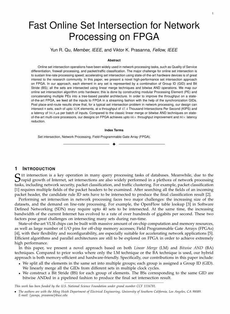
Fig. 1: An example of intersecting M = 3 sets, where all the elements are represented by IDs.

• We prototype our design on a state-of-the-art FPGA device. We present various tradeoffs on designparameters; we compare the performance of our designs in this paper with software-based set intersectionengines.

• We sustain 47.4 KIPS throughput when intersecting 8 sets, each of upto 32 K elements. Compared to theclassic LM technique or BA technique on state-of-the-art multi-core processors, our approach achievesupto 66× throughput improvement and 80× latency reduction.

The rest of the paper is organized as follows: We introduce the background and related works in Section 2.We present our novel data structures and algorithms in Section 3. We implement our set intersection engineon FPGA in Section 4. We evaluate the performance in Section 5 and conclude the paper in Section 6.

2 BACKGROUND

2.1 NotationsSet intersection is a well-known operation to select common elements in all the given sets. In this paper, weassume, without loss of generality, that the elements in each set are presorted in ascending order. We denotethe number of sets to be intersected as M . We denote the number of elements in each set as Nm, wherem = 0, 1, . . . ,M −1. We show an example of M = 3 in Figure 1, where N0 = 5, N1 = 3, and N2 = 4. We denotethe final intersected set as I ; in the example shown in Figure 1, I = 5, 103.

We use argminm

Nm as the index of the smallest set, where argminm

Nm ∈ 0, 1, . . . ,M−1. Similarly, argmaxm

Nm

can be defined. Assuming the element IDs use natural numbers, we denote the largest element in any set as(Ω− 1). In Figure 1, argmin

mNm = 1, argmax

mNm = 0, and Ω = 256.

2.2 ApproachesSet intersection has been widely studied in both database systems [6], [7] and network processing [8]–[10]. Ingeneral, there are two major categories for set intersection approaches: (1) the LM techniques, and (2) the BAtechniques.

The classic LM technique requires the elements in each set to be represented by IDs, each of log Ω bits;the common elements appearing in all the sets can be identified by iteratively checking the smallest/largestelements in all the sets [10]. This technique requires O (

∑Nm log Ω) memory and O (

∑Nm log Ω) time com-

plexity.An enhanced version [7] of the LM technique can be much more complex, where the elements in the

smallest set are used to eliminate the candidates in all the other sets. The memory consumption for thisenhanced version is O (

∑Nm log Ω), while the time complexity for intersecting all the M sets is

O

∑m 6=argmin

mNm

log (Nm log Ω)

(1)

The major drawback of the LM techniques is that it is not easy to implement such algorithms in a streamingfashion on hardware. A single intersection on M sets introduces processing latency of multiple clock cycles.

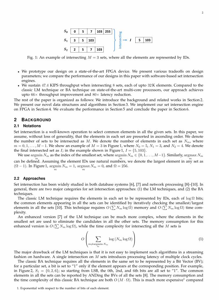
The classic BA technique requires all the elements in the same set to be represented by a Bit Vector (BV);for a particular set, a bit is set to “1” only if the element appears at the corresponding position. For example,in Figure 2, S1 = 0, 2, 6; so starting from LSB, the 0th, 2nd, and 6th bits are all set to “1”. The commonelements in all the sets can be reported by ANDing the BVs of all the sets [8]. The memory consumption andthe time complexity of this classic BA technique are both O (M · Ω). This is much more expensive1 compared

1. Exponential with respect to the number of bits of each element.

3

0 1 1 0 1 1 0 1𝑺𝟎

𝑺𝟏

𝑺𝟐

0 1 0 0 0 1 0 1

0 0 1 1 1 1 1 1

&

&

0 0 0 0 0 1 0 1𝑰

intersecting

Fig. 2: An example of intersecting M = 3 sets, where all the sets are represented by BVs.

Set intersection

engine

𝑰

𝑺𝟎

𝑺𝟏

𝑺𝑴−𝟏

FPGA

Set intersection

engine

𝑰

Index to 𝑺𝟎

Index to 𝑺𝟏

Index to 𝑺𝑴−𝟏

FPGA

memory

memory

memory

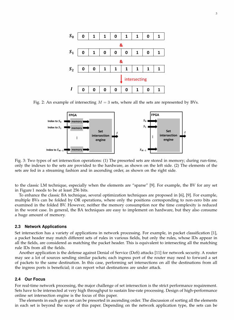
……Fig. 3: Two types of set intersection operations: (1) The presorted sets are stored in memory; during run-time,only the indexes to the sets are provided to the hardware, as shown on the left side. (2) The elements of thesets are fed in a streaming fashion and in ascending order, as shown on the right side.

to the classic LM technique, especially when the elements are “sparse” [9]. For example, the BV for any setin Figure 1 needs to be at least 256 bits.

To enhance the classic BA technique, several optimization techniques are proposed in [6], [9]. For example,multiple BVs can be folded by OR operations, where only the positions corresponding to non-zero bits areexamined in the folded BV. However, neither the memory consumption nor the time complexity is reducedin the worst case. In general, the BA techniques are easy to implement on hardware, but they also consumea huge amount of memory.

2.3 Network ApplicationsSet intersection has a variety of applications in network processing. For example, in packet classification [1],a packet header may match different sets of rules in various fields, but only the rules, whose IDs appear inall the fields, are considered as matching the packet header. This is equivalent to intersecting all the matchingrule IDs from all the fields.

Another application is the defense against Denial of Service (DoS) attacks [11] for network security. A routermay see a lot of sources sending similar packets; each ingress port of the router may need to forward a setof packets to the same destination. In this case, performing set intersections on all the destinations from allthe ingress ports is beneficial; it can report what destinations are under attack.

2.4 Our FocusFor real-time network processing, the major challenge of set intersection is the strict performance requirement.Sets have to be intersected at very high throughput to sustain line-rate processing. Design of high-performanceonline set intersection engine is the focus of this paper.

The elements in each given set can be presorted in ascending order. The discussion of sorting all the elementsin each set is beyond the scope of this paper. Depending on the network application type, the sets can be

4

GID BS

10000 0111

00001 1110

00000 1101

GID BS

11111 0001

00100 0100

00001 1011

Comparator (=)

Bitwise AND

Elements of 𝑆0 Elements of 𝑆1

GID BS

00100 0100

00001 1000

Elements of 𝑆2

55

5

4

4

45

4

𝒎 = 𝟎 𝒎 = 𝟏 𝒎 = 𝟐

GID BS

00001 1000

EN

Fig. 4: Using GID and BS for set intersection. In this example, there are M = 3 sets, g = 5 bits per GID, ands = 4 bits per BS. After groups are intersected, an enable signal EN is generated to control the bitwise ANDoperations for the corresponding BSs.

prepared during design-time [1], or provided as inputs during run-time [11]. This leads to two slightly differenthardware implementations, as shown on the left side and right side of Figure 3, respectively. In this paper,since our focus is the high-performance set intersection engine, we assume all the elements of the sets areonly known during run-time; hence we choose the implementation type as shown on the right hand side ofFigure 3.

3 DATA STRUCTURES AND ALGORITHMS

3.1 MotivationsAs can be seen, the LM techniques are memory-efficient for sparse sets, while the BA techniques are easy forhardware implementation. This observation inspires us to exploit a hybrid data structure. The basic ideas are:

1) We split all the elements into multiple groups; each group in a set is assigned a unique Group ID (GID).All the sets are intersected on GIDs first, using the LM techniques.

2) We associate each GID with a shorter Bit Stride (BS); each bit in the BS corresponds to an element in aset. For different sets, only the BSs corresponding to the same GIDs are ANDed.

Since all the sets are represented in GIDs and BSs, we define this representation of data structures as GID/BSrepresentation.

3.2 GID/BS representationWe denote the number of bits for a GID as g. We denote the number of bits in a BS as s. Based on the notationsintroduced in Section 2.1, each long BV in the classic BA technique can use upto Ω bits. To reduce the memoryconsumption, we split each BV into a total number of Ω

s groups, each of s bits. Hence each group correspondsto an s-bit BS. We assign a GID to a group. The GIDs are unique in each set, but the GIDs in different setscan be identical.

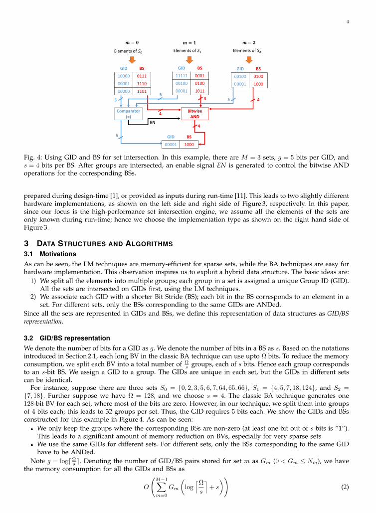
For instance, suppose there are three sets S0 = 0, 2, 3, 5, 6, 7, 64, 65, 66, S1 = 4, 5, 7, 18, 124, and S2 =7, 18. Further suppose we have Ω = 128, and we choose s = 4. The classic BA technique generates one128-bit BV for each set, where most of the bits are zero. However, in our technique, we split them into groupsof 4 bits each; this leads to 32 groups per set. Thus, the GID requires 5 bits each. We show the GIDs and BSsconstructed for this example in Figure 4. As can be seen:• We only keep the groups where the corresponding BSs are non-zero (at least one bit out of s bits is “1”).

This leads to a significant amount of memory reduction on BVs, especially for very sparse sets.• We use the same GIDs for different sets. For different sets, only the BSs corresponding to the same GID

have to be ANDed.Note g = logdΩ

s e. Denoting the number of GID/BS pairs stored for set m as Gm (0 < Gm ≤ Nm), we havethe memory consumption for all the GIDs and BSs as

O

(M−1∑m=0

Gm

(log⌈Ω

s

⌉+ s

))(2)

5

For s = 1, this memory requirement is the same as the classic LM technique. For s = Ω, this memoryrequirement is the same as the classic BA technique. We will discuss the time complexity of our set intersectionalgorithm in Section 4. We will also determine the value of s later in Section 5.

3.3 Online Set Intersection

Algorithm 1 Online Set Intersection

Input A total number of M sets Sm, m = 0, 1, . . . ,M − 1, represented using the GID/BS representation.Output An intersected set I , whose entries are indexed by i. ∀i, ∀m, GID[i] = GID[m, im] for some im; BS[i] =

BS[0, i0] & BS[1, i1] & . . . & BS[M−1, iM−1] where GID[i] = GID[0, i0] = GID[1, i1] = · · · = GID[M−1, iM−1].1: for m = 0 to M − 1 do2: im ← 0 pointers initialization3: end for4: i← 0 pointer for I5: while (i0 < G0) || (i1 < G1) ||

. . . || (iM−1 < GM−1) do6: X ← GID[0, i0] set current maximum7: for m = 0 to M − 1 do8: if GID[m, im] > X then9: flag ← false reset flag

10: X ← GID[m, im] elements not equal11: else if GID[m, im] < X then12: flag ← false reset flag13: if im < Gm then14: im ← im + 1 advance index15: else16: go to Step 3717: end if18: else19: if m = 0 then20: flag ← true set flag for S021: else if m = M − 1 then22: if flag = true then23: flag ← false elements equal24: GID[i]← GID[0, i0]25: BS[i]← BS[0, i0]26: i0 ← i0 + 1 advance index27: for m′ = 1 to M − 1 do28: BS[i]← BS[i] & BS[m′, im′ ]29: im′ ← im′ + 1 advance index30: end for31: i← i+ 132: end if33: end if34: end if35: end for36: end while37: report I consisting of GID[i], BS[i], where i = 0, 1, . . . , P − 1

Our set intersection approach consists of two phases as follows:1) Preprocessing: all the sets are preprocessed using the GID/BS representation. This phase can be done

offline.2) Online Set Intersection: all the GIDs are intersected for different sets; their corresponding BVs are bitwise

ANDed.As discussed in Section 2.4, we assume the elements in each given set are already sorted in ascending order,

thus, we ignore the discussion of the preprocessing phase in this paper. We focus on the online set intersectionphase in this section.

6

FIFO_0

FIFO_1

GIDComparator

(=)

Bitwise AND

EN_R0

EN_R1

EN_W0

EN_W1

EN_W2

BS

GID

BS

GID

BS

Fig. 5: Internal organization of a modular PE. The data width of any GID is g bits. The data width of anyBS is s bits. The data width of any control signal (e.g., EN W0, etc.) is 1 bit. Other FIFO control signals areomitted for simplicity, e.g., not full, not empty, etc.

For set m, since there are Gm GID/BS pairs stored, we index them by im = 0, 1, . . . , Gm − 1; the GID andBS corresponding to index im are denoted as GID[m, im] and BS[m, im], respectively. For example, in Figure 4,for set S2, G2 = 2, and i2 = 0, 1. GID[2, 0] = 00100, BS[2, 0] = 0100, GID[2, 1] = 00001, and BS[2, 1] = 1000.Similarly, we assume the final intersected set I has P GID/BS pairs, indexed by i = 0, 1, . . . , P − 1; the GIDand BS in set I are denoted as GID[i] and BS[i].

We show our online set intersection algorithm in Algorithm 1. Figure 4 shows an example of the correspond-ing architecture. The smallest GIDs in all the M sets are compared against each other, and the GIDs smallerthan the maximum value (X , as denoted in Algorithm 1) are excluded from I . Only if all the smallest GIDs inall the sets are equal, have we identified a common GID in all the M sets; in this case, the corresponding BSsare ANDed. In other words, the GIDs are intersected using an LM-like technique, while the BSs correspondingto the same GIDs are intersected using bitwise AND operations.

4 HARDWARE ARCHITECTURE

The architecture shown in Figure 4 is naive, because there are several drawbacks to be noticed:1) The performance of comparing GIDs and bitwise ANDing BSs deteriorates as M increases; intersecting

a large number of sets can lead to very slow clock rate.2) Intersecting GIDs may require multiple clock cycles to complete; this degrades the overall throughput

performance of the architecture.In this section, we will improve the performance of our hardware architecture on FPGA using (1) modularProcessing Element (PE) (Section 4.1), and (2) tree-based parallel architecture (Section 4.2). We present a streamingtechnique to feed different batches (see Section 4.3) of data back-to-back; our intention is to achieve very highthroughput by minimizing the communication overheads between different batches of data.

4.1 Modular PEWe show the internal organization of a modular PE in Figure 5. A modular PE takes GIDs and BSs from twoordered sets; the GIDs and BSs are fed in ascending order into the PE. The basic operations of a modularPE consist of reporting common GIDs, and performing bitwise AND operations on the corresponding BSs.Specifically, a modular PE contains the following components: 2 FIFOs, one g-bit comparator, and one s-bitbitwise AND gate.

4.1.1 2 FIFOsThe FIFOs are used to buffer the GID/BS pairs. The write enable signals EN W0 and EN W1 are fed fromthe inputs. The read enable signals EN R0 and EN R1 are generated internally by the comparator.

4.1.2 g-bit ComparatorThe comparator compares two GIDs, each of g bits. Based on the comparison result, the comparator generates3 control signals:

1) On the one hand, if two GIDs are identical, the comparator sets EN W2 = 1 for the next PE to acceptthis GID and the corresponding ANDed BS. To compare the next two GIDs, both EN R0 and EN R1 areset to 1 for the two FIFOs.

7

TABLE 1: Truth table for the control signals (assuming neither of the FIFO is empty)

Case Equal GIDsGID in FIFO 0 GID in FIFO 1

is smaller is smaller

EN R0 1 1 0EN R1 1 0 1EN W2 1 0 0

PE

PE

PE

From Set 𝑺𝟎

From Set 𝑺𝟏

From Set 𝑺𝟐

From Set 𝑺𝟑

Set 𝑰

Level 0 Level 1

Fig. 6: An example of tree-based architecture: M = 4 sets are intersected using 2 levels of PEs.

2) On the other hand, if two GIDs are not equal, the comparator sets EN W2 = 0. Since we only keep trackof the maximum value of the smallest elements in two sets, out of the two GIDs, the smaller one isdiscarded; hence, only one of EN R0 and EN R1 is set to 1 for the corresponding FIFO to provide thenext GID.

We summarize the values of the control signals generated by the g-bit comparator in Table 1.

4.1.3 s-bit Bitwise AND GateThe bitwise AND gate perform bitwise AND operations on two BSs, each of s bits. The result is an ANDedBS, consisting of s bits. Although the bitwise AND gate produces results for any two compared GIDs, thecontrol signal EN W2 decides whether the result produced by this gate should be accepted by the next PE.The ANDed BS is only accepted when the two GIDs compared are identical, as shown in Table 1.

4.2 Tree-based Parallel ArchitectureThe modular PE discussed in Section 4.1 only intersects 2 sets. To intersect a large number of sets, multiplemodular PEs have to be used. Also, to reduce the processing latency, parallel architectures have to be exploited.Our intuition in this paper is to intersect M sets iteratively, two sets at a time using the modular PE inSection 4.1.

For M sets, we choose to deploy logM levels of PEs; for instance, M = 4 in Figure 6, so 2 levels of PEsare deployed. In our notations, level 0 always consists of all the leaves of the tree, where level (logM − 1)consists of only the root of the tree. We denote this architecture as tree-based parallel architecture, because (1)all the PEs are connected in a tree-like fashion, and (2) all the PEs at the same level perform set intersectionsin parallel.

In our architecture, we notice that the size of the intersection of any two sets is no greater than the size ofthe smaller set; as we go towards the root, smaller and smaller FIFOs can be used. The clock rate supportedby the PE at the root is no slower than the clock rates supported by the PEs at the leaves.

The naive architecture shown in Figure 4 leads to a time complexity (or processing latency) of

O

(M−1∑m=0

Gm

(log⌈Ω

s

⌉+ s))

∼ O(M ·max

m[Gm]

(log⌈Ω

s

⌉+ s))

(3)

where Gm (0 < Gm ≤ Nm) denotes the number of GID/BS pairs stored for set m.However, using our tree-based parallel architecture introduced in this section, we can intersect M sets with

a (parallel) time complexity of

O

((logM

)·max

m[Gm] ·

(log⌈Ω

s

⌉+ s))

(4)

8

10

9

7

5

2

10

7

3

2

PE

10

7

2

10

9

7

255

5

2

10

255

7

3

2

PE

10

255

2

Ad

din

g sy

nc.

GID

(Wro

ng

resu

lt)

(Co

rre

ct r

esu

lt)

Fig. 7: Adding synchronization GIDs, where g = 8 and M = 2. Red numbers denote synchronization GIDs,while black numbers denote regular GIDs.

Note that this upperbound is quite a loose upperbound. As discussed, this is because the number of commonelements in two sets is no more than the number of elements in the smaller set; we have (possibly) smallerand smaller sets to be merged linearly as we go down towards the tree root.

4.3 Streaming InputsOur architecture can intersect M sets at a time. We denote such M sets to be intersected as a batch. For example,in Figure 7, suppose a batch of two sets, consisting of GIDs 2, 5 and GIDs 2, 3, 7, are to be intersected;another batch of two sets, consisting of GIDs 7, 9, 10 and GID 10, are to be intersected. Using a singlemodular PE, we need to generate the correct results consisting of GID 2 and GID 10 sequentially.

In our architecture, all the GID/BS pairs can be streamed in; this means the time for getting GIDs fromdifferent batches can be overlapped. This benefits the throughput performance. However, the inputs fromdifferent batches need to be distinguished to avoid any confusion; otherwise the intersected result can bewrong. Continuing the example discussed above, we show the wrong results generated from two batches ofinputs on the left side of Figure 7.

We employ synchronization GID to separate GIDs from different batches. As opposed to regular GIDs, asynchronization GID is a GID with all of its g bits set to 1. A synchronization GID is forbidden in theinput; meanwhile, all of the synchronization GIDs in the final output2 are discarded. Continuing the examplediscussed in this subsection, we show how we generate the correct intersected sets using synchronizationGIDs in Figure 7. As can be seen in this figure, since g = 8, we add the synchronization GID 255 immediatelyafter the end of the first batch; note that the same synchronization GID must be added to all the M sets (inthis example, M = 2). The synchronization GID is an overhead for streaming inputs:• Time overhead: it takes 1 extra clock cycle to synchronize all the sets of the same batch.• Resource overhead: the synchronization GID uses g bits itself; also, the corresponding s-bit BS cannot be

utilized for this GID.We add synchronization GIDs during the preprocessing phase; thus, the synchronization GIDs are streamedin just like all the other regular GIDs.

5 EVALUATION

We organized this section as follows:• In Section 5.1, we introduce the setups of our experiments.• In Section 5.2, we determine the values of g and b by investigating their effect on the hardware perfor-

mance.• In Section 5.3, we examine the impact of various values of Ω on the performance with respect to through-

put, latency, resource utilization, and power.• In Section 5.4, we examine the impact of various values of M on the performance with respect to through-

put, latency, resource utilization, and power.

2. Only at the root level of the tree-based architecture.

9

TABLE 2: Performance with respect to g and b (M = 4)

gb 2 4 8 16 32 64

2

Clock rate (MHz) 486.85 441.31 375.66 379.51 383.58 312.50Logic slices (%) 0.01 0.01 0.02 0.02 0.04 0.07

BRAM (%) 0.00 0.00 0.00 0.00 0.00 0.00I/O pins (%) 2.90 3.81 5.63 9.27 16.54 31.09

4


BRAM (%) 0.00 0.00 0.00 0.00 0.00 0.31I/O pins (%) 3.81 4.72 6.54 10.18 17.45 32.00

6


BRAM (%) 0.00 0.00 0.00 0.15 0.15 0.31I/O pins (%) 4.72 5.63 7.45 11.09 18.36 32.90

8


BRAM (%) 0.00 0.15 0.15 0.15 0.15 0.31I/O pins (%) 5.63 6.54 8.36 12.00 19.27 33.81

10


BRAM (%) 0.15 0.15 0.15 0.15 0.31 0.63I/O pins (%) 6.54 7.45 9.27 12.90 20.18 34.72

12


BRAM (%) 0.15 0.15 0.31 0.63 1.27 2.39I/O pins (%) 7.45 8.36 10.18 13.81 21.09 35.63

• In Section 5.5, we evaluate the performance of our set intersection engine using real-life datasets.• In Section 5.6, we compare our work with prior works on various platforms.

5.1 Experimental Setup5.1.1 Hardware and SoftwareWe conducted experiments on the state-of-the-art Xilinx Virtex 7 FPGA (XC7VX1140T-FLG1930 -2L) [4]. ThisFPGA has 218800 logic slices, 1100 I/O pins, and 68 Mb BRAM; it can be configured to realize a large amountof distributed RAM (distRAM, upto 18 Mb). To simplify our designs, we instantiated all the memory modules(e.g., FIFO) using single-port distRAM or BRAM. We evaluated the performance using Xilinx Vivado 2014.2design tool [12].

5.1.2 Performance MetricsThe following performance metrics were considered in our experiments:

– Throughput: the number of intersected sets (I) produced per unit time (in KIPS). We recorded thethroughput values based on the clock rates from the post-place-and-route timing reports.

– Latency: the processing time required for intersecting M sets of the same batch. We reported the latencyvalues based on simulation results.

– Resource Utilization: the percentages of basic FPGA resources utilized. We investigated (1) logic sliceutilization, (2) BRAM utilization, and (3) I/O pin utilization, based on the post-place-and-route resourceutilization reports.

– Power: the power consumption of an entire design on FPGA, including both static power and dynamicpower. We fixed the temperature at 25 C. We used Switching Activity Interchange Format (SAIF) files asinputs to Vivado power analysis tool.

Throughput and resource utilization are very commonly used for most FPGA-based implementations [2], [5].Latency has regained much attention nowadays in SDN [3]. Power is a very important metric, especially forlarge data centers.

In addition, for throughput, we further defined:

10

– Peak throughput (Tpeak): the throughput determined by the hardware architecture for a given set ofdesign parameters (e.g., M , g, etc.). When calculating the peak throughput, we assume the FIFOs in thePEs are full for worst-case analysis.

– Sustained throughput (Tsustained): the throughput measured for a specific data trace. The sustainedthroughput varies during run-time, because the number of GID/BS pairs buffered in the FIFOs dependson the data trace.

The sustained throughput is hard to measure; we defer the discussion of the sustained throughput until latersections. For a given design, the peak throughput mainly depends on (1) the clock rate achievable on FPGAand (2) the size of the largest set to be intersected. Let f denote the maximum frequency achievable for adesign. Considering the time overhead on synchronization GIDs, we have:

Tpeak =f

maxm

[Gm] + 1(5)

5.1.3 DatasetsWe conducted extensive experiments on the real datasets from the classic 5-field packet classification problem[1], due to the availability of the rule sets and the packet traces [13]. Assuming all the 5 sets from the samepacket header had already been obtained, we only focused on intersecting M = 5 sets in this paper3. In orderto make all the implementations “modular”, for M = 5, we designed our intersection engines to take inputdata from at most 8 sets concurrently; i.e., all the values of M were rounded up to the nearest power of 2.

For real-life datasets in the 5-field packet classification, the largest real-life rule set, to the best of ourknowledge, had 32 K rules [13]; i.e., Ω = 32 K in this case. To measure the sustained throughput, we categorizeddifferent packet traces [13] based on the values of max

m

[Gm

]. We conduct 10 runs (as examples) for each

category; each run performs 10 K set intersections.To investigate the sustained throughput, we defined selectivity (denoted as η) to be the ratio of the size of

the intersection to the size of the largest set to be intersected:

η =|I|

maxm

[Gm](6)

As can be seen later, η has significant impact on the throughput and latency performance4.

5.2 Determining ParametersThere are many ways to determine the values of g and b. For instance, our approach exploits the LM techniques,which is a data-dependent algorithm. For a specific data trace, there may exist an “optimal” combination ofg and b, which gives the highest throughput or lowest processing latency. However, at the design time, weusually don’t know the statistics of the input data; the input data can also be purely random. In such cases, itis impossible to always use the “optimal” values of g and b. In this paper, we assume very little informationon the input data is known at the design time; thus, we determine the values of g and b based on the hardwareperformance.

5.2.1 FIFO depthThe maximum value of Gm is no greater than (2g − 1), because for any set m, the maximum number ofpossible g-bit GIDs is (2g − 1), excluding the synchronization GID as discussed in Section 4.3.

There is no direct relation between the FIFO depth and the values of Gm. For simplicity, we use a FIFOdepth greater than (2g − 1); this ensures that there is no data drop for the same batch of streaming inputs.In the tree-based parallel architecture as introduced in Section 4.2, the FIFOs in the PEs at various levels mayrequire different FIFO depths; however, in this paper, we simply use the same FIFO depth for all the levels.

To summarize, the relationship between the FIFO depth, the value of g, and the value of Gm, m =0, 1, . . . ,M − 1 in this paper can be described as:

FIFO depth > 2g − 1 ≥ maxm

[Gm

](7)

When conducting experiments, we always follow the relation indicated in Equation 7 in this paper.

3. The packet classification problem also involves searching all the fields to get all the sets before intersecting all the sets.4. In [7], selectivity was defined to be the ratio of the size of the intersection to the size of the smallest set. However, they are very

similar definitions and have similar impact on the performance.

11

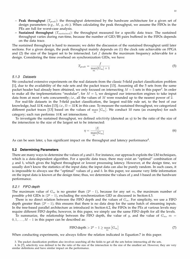
TABLE 3: Performance for various combinations of g and b, where Ω = 32 K, M = 8

g 11 12 13 14b 16 8 4 2

Clock (MHz) 222.52 261.23 196.19 180.54slices (%) 0.80 2.50 5.72 0.25

BRAM (%) 1.06 0.74 0.74 5.95I/O (%) 23.90 18.18 15.72 14.90

5.2.2 g and bTo determine the values of g and b, we first fix M = 4 as an example; similar trends can be seen for othervalues of M . We fix the depth of all the FIFOs in the modular PEs to be 2g ; thus, large values of g result indeep FIFOs. We show the clock rate achieved by our design and the corresponding resource consumption inTable 2. As can be seen:• Since both M and the FIFO depth are small, our designs utilize very small amounts of logic and memory

resources.• As the values of g increases, the clock rate usually degrades. Since the memory resources (distRAM

and BRAM) on FPGA are organized in modules, deep FIFOs require a large number of modules to beconnected by long wires.

• As the values of b increases, the clock rate also degrades. Since each PE in our designs performs ANDoperations in every clock cycle, it requires longer clock period to AND wide BSs.

• As the values of g or b increases, there are very few cases where the clock rate varies. The small variationsare caused by the design suite.

As can be seen in Table 2, the best clock rate is achieved at b = 4 or b = 8 in most cases; this is because forb = 4 or b = 8, very short BSs are ANDed in each PE, resulting in compact circuits and short wire lengths.Hence we tend to use small values of b in all of our experiments. Recalling Section 3.2, we have g = logdΩ

s e;therefore we choose the values of g based on both values of b and Ω.

5.2.3 Case StudyLet us study the case where Ω = 32 K and M = 8 as an example; we follow the same design methodology forother values of g, b, Ω, and M in this paper. Since we tend to use small values of b, we restrict b to be 2, 4,8, and 16. The corresponding values of g are 11, 12, 13, and 14, respectively. Under these configurations, weshow the performance with respect to the clock rate and the resource utilization in Table 3. As can be seen,the best clock rate is achieved when g = 12 and b = 8; this matches our conclusion in Section 5.2.2 that thebest clock rate is achieved when b = 4 or b = 8.

Note in Table 3, as the value of g increases, there are variations with respect to the utilization of logic slicesand BRAM. This is because we do not put any restrictions on the memory type (distRAM or BRAM) of theFIFOs; instead, we relay on the Vivado design suite to choose the memory type for best performance. A simplecalculation reveals that as g increases, the total memory consumption still increases.

5.3 Varying Ω

5.3.1 Throughput and LatencyUsing b = 8 and M = 8 as our configuration, we show the peak throughput and the corresponding latencywith respect to various values of g in Figure 8. For b = 8 and g = 11, 12, 13, 14, the corresponding values of Ωare 16 K, 32 K, 64 K, and 128 K, respectively; these values are sufficiently large for network applications [10]. Asthe value of g increases, the FIFO depth increases exponentially; the peak throughput tapers while the latencyincreases dramatically. The reason is that our set intersection approach still employs the LM techniques, whosetime complexity is linear with respect to max

m

[Gm

](or 2g in this paper, because of Equation 7).

5.3.2 Resource UtilizationIn Figure 9, we show the corresponding resource utilization with respect to (1) the logic slices, (2) BRAM, and(3) I/O pins on FPGA. As can be seen, the I/O pin utilization increases slightly as g increases; this matchesour intuition because each input GID/BS pair requires (g + b) input pins. There are variations with respect tothe logic slice utilization and BRAM utilization; this also matches our observation discussed in Section 5.2.3.

12

0

100

200

300

400

0

25

50

75

100

11 12 13 14

Late

ncy

(µ

s)

Pe

ak T

hro

ugh

pu

t (K

IPS)

No. of Bits per GID (g)

Throughput Latency

Fig. 8: Peak throughput for b = 8, and M = 8

0.7

9%

2.5

0%

5.7

2%

0.2

6%

0.6

9%

0.7

4%

1.4

8%

8.1

9%

17

.36

%

18

.18

%

19

.00

%

19

.81

%

0%

25%

50%

75%

100%

11 12 13 14

Uti

lizat

ion

(%

)


Logic slice BRAM I/O

Fig. 9: Resource utilization for b = 8, and M = 8

5.3.3 Power ConsumptionIn Figure 10, we show the corresponding power consumption. As can be seen, the static power consumptionvaries little while the dynamic power consumption increases as g increases.

The trends shown in Figure 8, Figure 9, and Figure 10 can be observed for other combinations of b and Mas well. Again, most of our designs on FPGA only consume very few logic slices, which is consistent with theresults shown in Table 2. This is an advantage because the remaining logic slices can be used to implementother database kernels besides set intersection.

5.4 Varying M

5.4.1 Throughput and LatencyTo examine the effect of M on the performance, we still use Ω = 32 K as an example, although similar trendscan be seen for other values of Ω as well. Varying M , we show the peak throughput and the “worst-case”latency in Figure 11, and Figure 12, respectively.

As can be seen in Figure 11 and Figure 12, as M increases, the peak throughput and the worst-case latencydeteriorate; this is because the clock rate degrades as M increases. For larger values of M , more resources areutilized, leading to less routing choices, longer wire lengths, and slower clock rates (see Section 5.4.2).

We have two important observations in Figure 11 and Figure 12:• The peak throughput and the worst-case latency are dominated by the largest size of the sets to be

intersected (2g).• M only has limited impact on the performance, especially when 2g is large.

As can be seen in Equation 4, in each FIFO, all the 2g GID/BS pairs buffered have to be checked in the worstcase, leading to a time complexity of O (2g). This explains why the peak throughput is halved and the worst-case latency is doubled each time as g increases. This matches our intuition in Equation 4: our tree-based

13

0

1

2

3

4

11 12 13 14P

ow

er

(W)


Static Dynamic

Fig. 10: Power consumption for b = 8, and M = 8

0

50

100

150

200

2 4 8 16

Pe

ak T

hro

ugh

pu

t (K

IPS)

No. of Sets (M)

g=11, b=16 g=12, b=8 g=13, b=4 g=14, b=2

Fig. 11: Peak throughput for Ω = 32 K

parallel architecture is in favor of intersecting a large number of small sets rather than intersecting very fewlarge sets.

5.4.2 Resource UtilizationIn Figure 13 and Figure 14, we can see that the total memory utilization increases with respect to M , in spiteof the variations with respect to the logic slice utilization or the BRAM utilization only. The reasons are thesame as discussed in Section 5.2.3.

Figure 15 show that, the total number of I/O pins available on FPGA bottlenecks the scalability of ourdesign, since intersecting a large number of M sets requires a large number of O(M) parallel input pins tobe used.

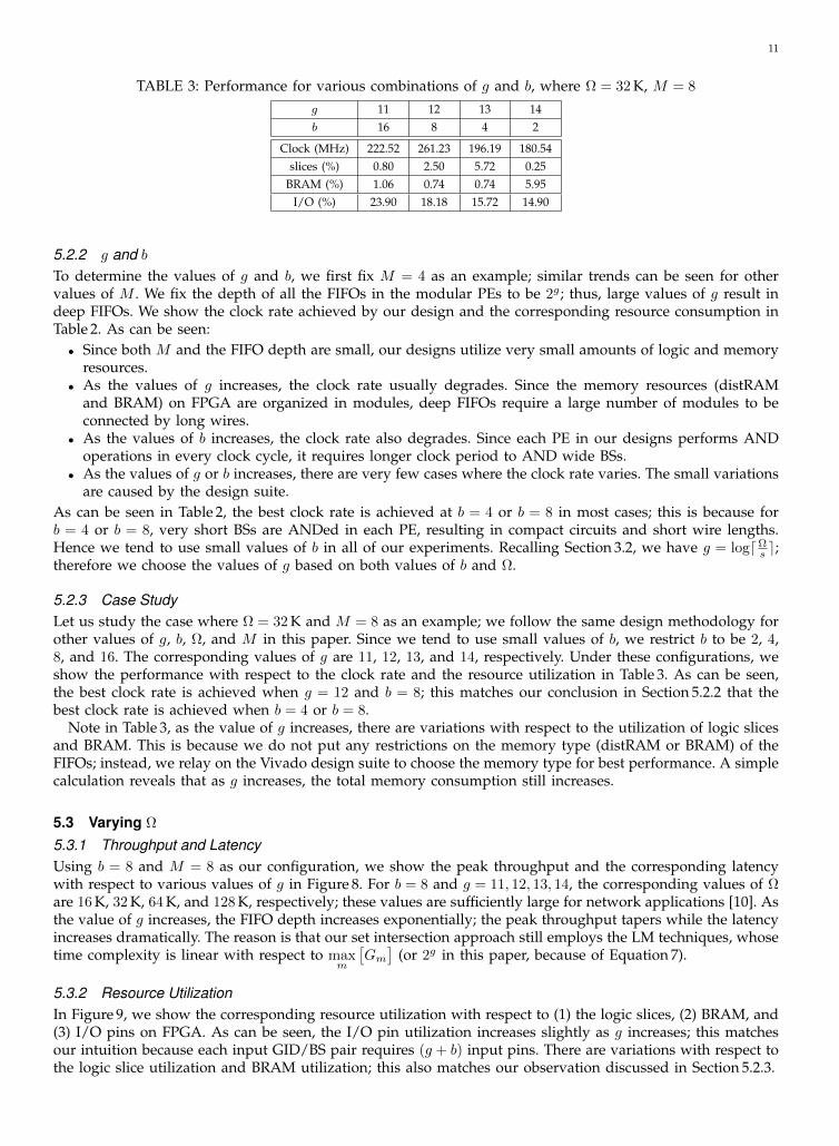
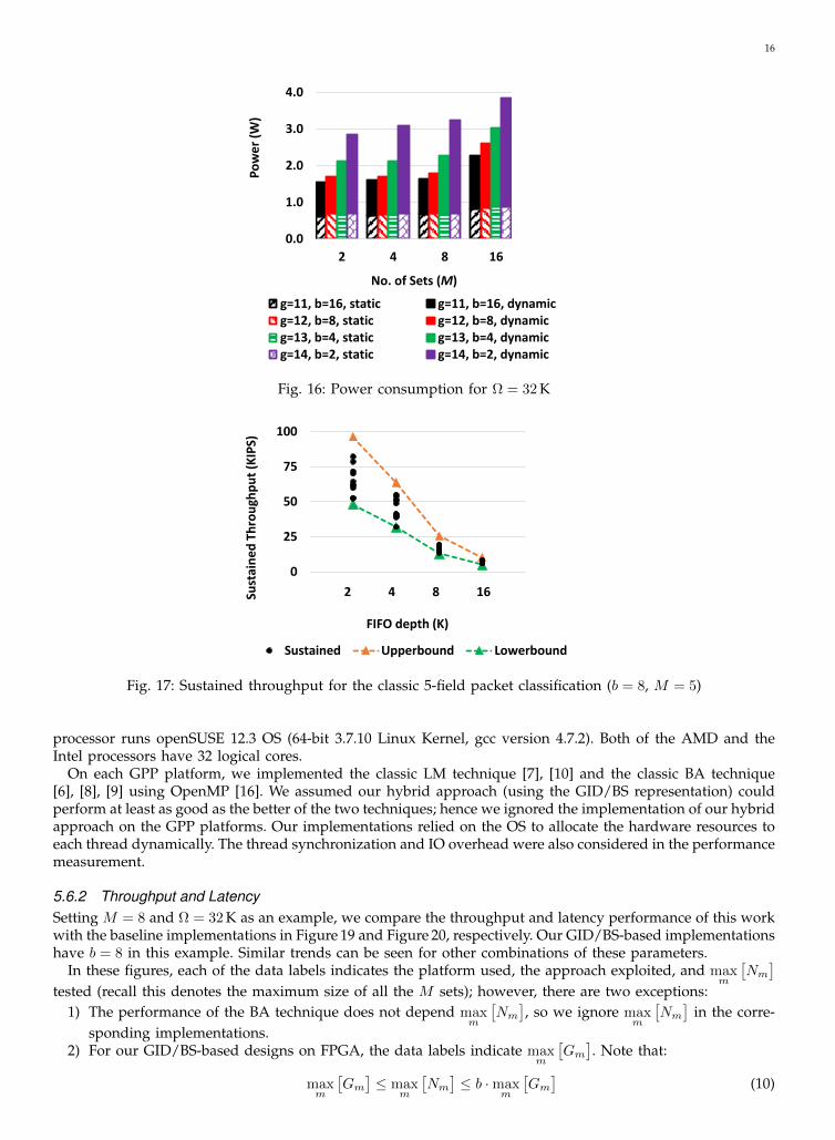
5.4.3 Power ConsumptionWe show the static power and dynamic power for Ω = 32 K in Figure 16, with respect to various combinationsof g and b. As can be seen:• As g increases, the dynamic power consumed by our designs increases linearly with respect to the total

memory consumption.• As M increases, the dynamic power consumed by our designs also increases linearly with respect to the

total memory consumption.• As g or M increases, the static power consumption only increases slightly.

Hence we observe that the total power consumption is almost linear with respect to the total memory utilized.This observation matches our intuition that the memory power dominates the total power consumption.

14

0

50

100

150

200

2 4 8 16La

ten

cy (

µs)

No. of Sets (M)

g=11, b=16 g=12, b=8 g=13, b=4 g=14, b=2

Fig. 12: Worst-case latency for Ω = 32 K

0.1

9%

0.5

6%

0.8

0%

1.0

2%

0.3

4%

1.0

5%

2.5

0%

0.4

0%

0.8

0%

2.4

4%

5.7

2%

0.4

4%

0.0

3%

0.1

1%

0.2

5%

0.5

1%

0%

25%

50%

75%

100%

2 4 8 16

Slic

e U

tiliz

atio

n (

%)

No. of Sets (M)

g=11, b=16 g=12, b=8 g=13, b=4 g=14, b=2

Fig. 13: Utilization of logic slices for Ω = 32 K

5.5 Real DatasetsIn this subsection, we use the real-life datasets in the 5-field packet classification to test our online setintersection engines, as introduced in Section 5.1.3.

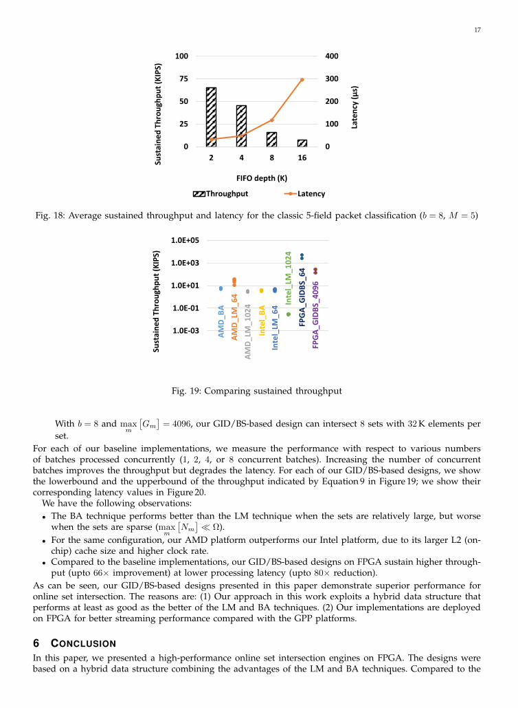
5.5.1 Throughput and LatencyFor a batch of M sets, the set intersection is not considered as complete unless all the GIDs have been examined(Gm GIDs for set m). In our tree-based parallel architecture, the sustained throughput is lowerbounded bythe throughput achieved at level 0 of the tree. We have

Tsustained ≥f

2 ·maxm

[Gm](8)

Besides, the sustained throughput is upperbounded by the peak throughput. Hence:

f

2 ·maxm

[Gm]≤ Tsustained ≤

f

maxm

[Gm] + 1(9)

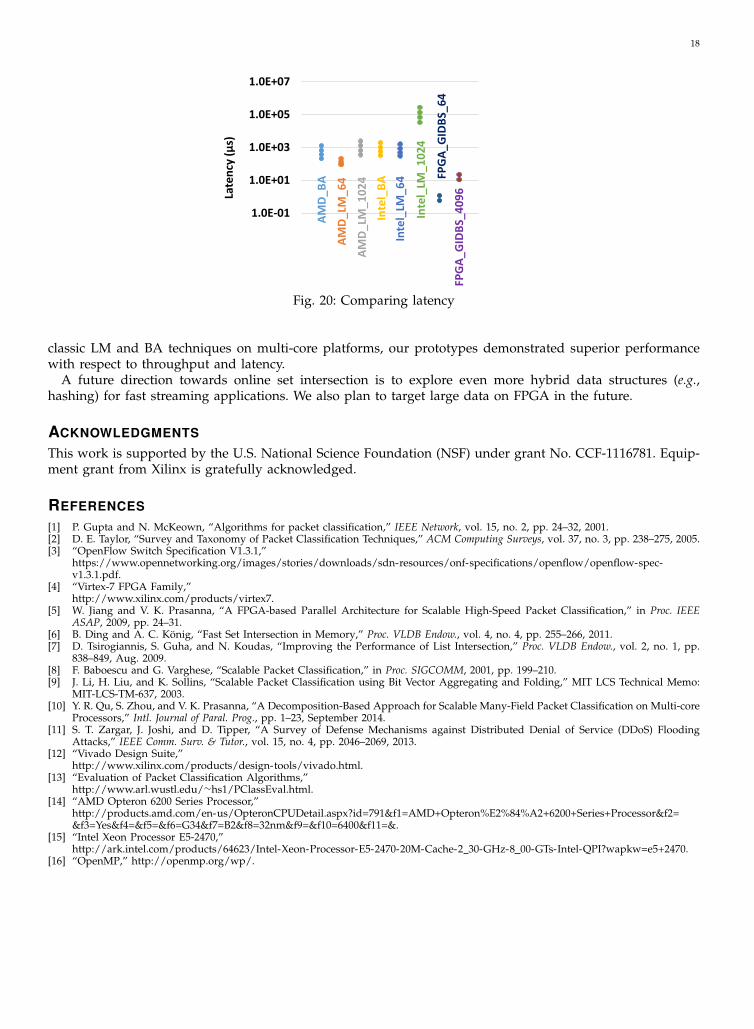
We show the sustained throughput with respect to various FIFO depths (from 2 K to 16 K) in Figure 17. Weindicate in this figure both the lowerbound and upperbound of the sustained throughput based on Equation 9.For each FIFO depth, we show the sustained throughput for 10 runs, each run corresponding to 10 K setintersections, as introduced in Section 5.1.3.

For each FIFO depth (10 runs), we show the average sustained throughput and the corresponding averagelatency in Figure 18. As max

m

[Gm

]increases, both the throughput and the latency deteriorate. Since it takes

linear time to merge all the GIDs in our approach, the performance with respect to throughput and latencyis adversely affected by max

m

[Gm

].

15

0.1

0%

0.3

1%

1.0

6%

2.7

6%

0.1

0%

0.3

1%

0.7

4%

3.9

8%

0.1

0%

0.3

1%

0.7

4%

7.1

8%

0.8

5%

2.5

5%

5.9

5%

12

.76

%

0%

25%

50%

75%

100%

2 4 8 16B

RA

M U

tiliz

atio

n (

%)

No. of Sets (M)

g=11, b=16 g=12, b=8 g=13, b=4 g=14, b=2

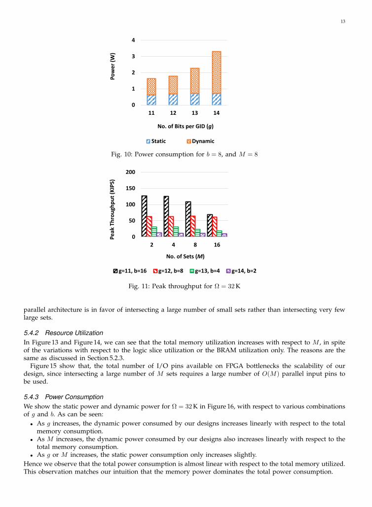
Fig. 14: Utilization of BRAM for Ω = 32 K

8.0

9%

13

.36

%

23

.90

% 45

.00

%

6.1

8%

10

.18

%

18

.18

% 34

.18

%

5.3

6%

8.8

1%

15

.72

%

29

.54

%

5.0

9%

8.3

6%

14

.90

%

28

.00

%

0%

25%

50%

75%

100%

2 4 8 16

I/O

Uti

lizat

ion

(%

)

No. of Sets (M)

g=11, b=16 g=12, b=8 g=13, b=4 g=14, b=2

Fig. 15: Utilization of I/O pins for Ω = 32 K

5.5.2 Resource Utilization and PowerFor real datasets, the performance with respect to resource utilization and power consumption are consistentwith Figure 9 and Figure 10:• The logic slice utilization increases linearly as the FIFO depth increases; the total resource utilization is

always kept under 25%.• Our designs only consume a small amount of power, due to the low resource utilization.

In spite of the same power performance as Figure 10, the energy performance on real datasets may vary; thisis because different datasets can introduce various values of processing latency.

5.6 Comparison with Prior Works5.6.1 BaselineTo the best of our knowledge, we are not aware of online set intersection engines on FPGA. Hence, to comparethis paper with prior works, we deployed software-based set intersection engines on state-of-the-art multi-coreGeneral-Purpose Processors (GPPs) as the baseline implementations. We conducted experiments on a 2× AMDOpteron 6278 processor [14] and a 2× Intel Xeon E5-2470 processor [15]. The AMD processor has 16 physicalcores, each running at 2.4 GHz. Each core is integrated with a 16 KB L1 data cache, 16 KB L1 instruction cache,and a 2 MB L2 cache. A 6 MB L3 cache (Last-Level Cache, LLC) is shared among all the 16 cores; all the coreshave access to 64 GB DDR3-1600 main memory. The AMD processor runs openSUSE 12.2 OS (64-bit 2.6.35Linux Kernel, gcc version 4.7.1). The Intel processor also has 16 physical cores, each running at 2.3 GHz. Eachcore has a 32 KB L1 data cache, 32 KB L1 instruction cache, and a 256 KB L2 cache. All the 16 cores sharea 20 MB L3 cache (Last-Level Cache, LLC), and they have access to 48 GB DDR3-1600 main memory. This

16

0.0

1.0

2.0

3.0

4.0

2 4 8 16P

ow

er

(W)

No. of Sets (M)

g=11, b=16, static g=11, b=16, dynamicg=12, b=8, static g=12, b=8, dynamicg=13, b=4, static g=13, b=4, dynamicg=14, b=2, static g=14, b=2, dynamic

Fig. 16: Power consumption for Ω = 32 K

0

25

50

75

100

Sust

ain

ed

Th

rou

ghp

ut

(KIP

S)

FIFO depth (K)

Sustained Upperbound Lowerbound

2 4 8 16

Fig. 17: Sustained throughput for the classic 5-field packet classification (b = 8, M = 5)

processor runs openSUSE 12.3 OS (64-bit 3.7.10 Linux Kernel, gcc version 4.7.2). Both of the AMD and theIntel processors have 32 logical cores.

On each GPP platform, we implemented the classic LM technique [7], [10] and the classic BA technique[6], [8], [9] using OpenMP [16]. We assumed our hybrid approach (using the GID/BS representation) couldperform at least as good as the better of the two techniques; hence we ignored the implementation of our hybridapproach on the GPP platforms. Our implementations relied on the OS to allocate the hardware resources toeach thread dynamically. The thread synchronization and IO overhead were also considered in the performancemeasurement.

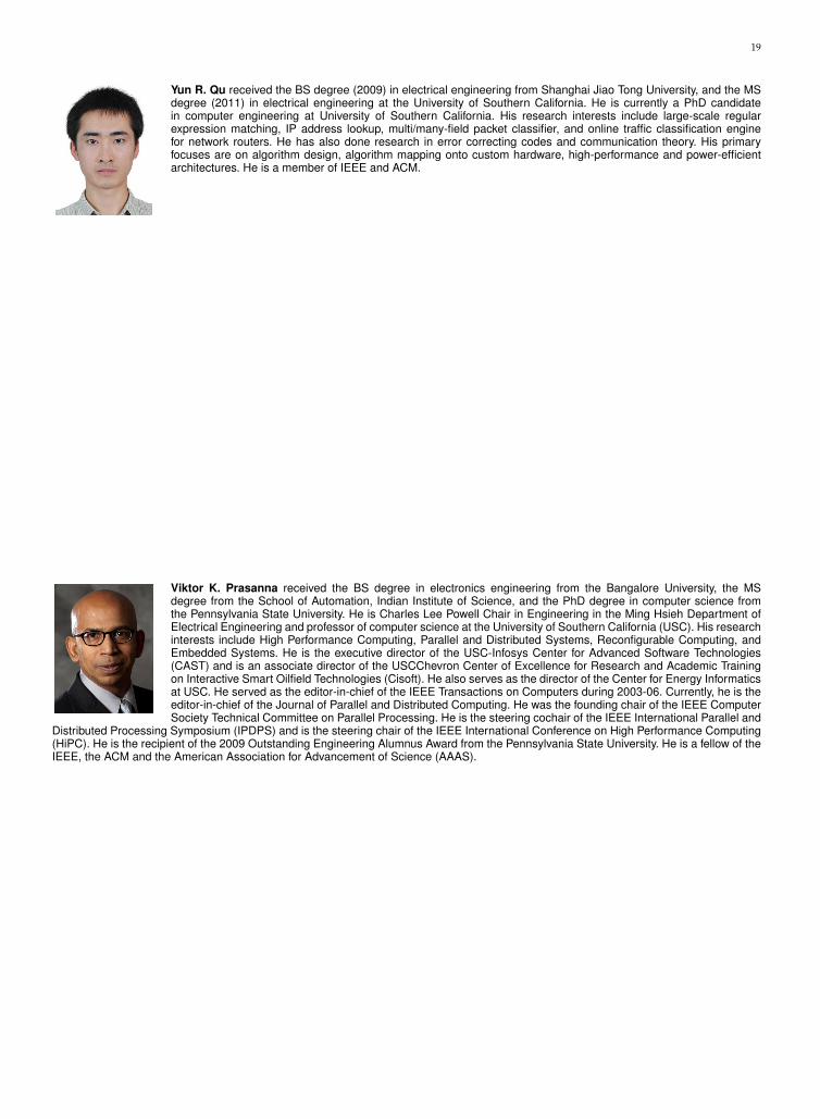
5.6.2 Throughput and LatencySetting M = 8 and Ω = 32 K as an example, we compare the throughput and latency performance of this workwith the baseline implementations in Figure 19 and Figure 20, respectively. Our GID/BS-based implementationshave b = 8 in this example. Similar trends can be seen for other combinations of these parameters.

In these figures, each of the data labels indicates the platform used, the approach exploited, and maxm

[Nm

]tested (recall this denotes the maximum size of all the M sets); however, there are two exceptions:

1) The performance of the BA technique does not depend maxm

[Nm

], so we ignore max

m

[Nm

]in the corre-

sponding implementations.2) For our GID/BS-based designs on FPGA, the data labels indicate max

m

[Gm

]. Note that:

maxm

[Gm

]≤ max

m

[Nm

]≤ b ·max

m

[Gm

](10)

17

0

100

200

300

400

0

25

50

75

100

2 4 8 16

Late

ncy

(µ

s)

Sust

ain

ed

Th

rou

ghp

ut

(KIP

S)

FIFO depth (K)

Throughput Latency

Fig. 18: Average sustained throughput and latency for the classic 5-field packet classification (b = 8, M = 5)

1.0E-03

1.0E-01

1.0E+01

1.0E+03

1.0E+05

Sust

ain

ed

Th

rou

ghp

ut

(KIP

S)

AM

D_B

A

AM

D_L

M_6

4

AM

D_L

M_1

02

4

Inte

l_B

A

Inte

l_LM

_64

Inte

l_LM

_10

24

FPG

A_G

IDB

S_6

4

FPG

A_G

IDB

S_4

09

6

Fig. 19: Comparing sustained throughput

With b = 8 and maxm

[Gm

]= 4096, our GID/BS-based design can intersect 8 sets with 32 K elements per

set.For each of our baseline implementations, we measure the performance with respect to various numbersof batches processed concurrently (1, 2, 4, or 8 concurrent batches). Increasing the number of concurrentbatches improves the throughput but degrades the latency. For each of our GID/BS-based designs, we showthe lowerbound and the upperbound of the throughput indicated by Equation 9 in Figure 19; we show theircorresponding latency values in Figure 20.

We have the following observations:• The BA technique performs better than the LM technique when the sets are relatively large, but worse

when the sets are sparse (maxm

[Nm

] Ω).

• For the same configuration, our AMD platform outperforms our Intel platform, due to its larger L2 (on-chip) cache size and higher clock rate.

• Compared to the baseline implementations, our GID/BS-based designs on FPGA sustain higher through-put (upto 66× improvement) at lower processing latency (upto 80× reduction).

As can be seen, our GID/BS-based designs presented in this paper demonstrate superior performance foronline set intersection. The reasons are: (1) Our approach in this work exploits a hybrid data structure thatperforms at least as good as the better of the LM and BA techniques. (2) Our implementations are deployedon FPGA for better streaming performance compared with the GPP platforms.

6 CONCLUSION

In this paper, we presented a high-performance online set intersection engines on FPGA. The designs werebased on a hybrid data structure combining the advantages of the LM and BA techniques. Compared to the

18

1.0E-01

1.0E+01

1.0E+03

1.0E+05

1.0E+07

Late

ncy

(µ

s)

AM

D_B

A

AM

D_L

M_6

4

AM

D_L

M_1

02

4

Inte

l_B

A

Inte

l_LM

_64

Inte

l_LM

_10

24

FPG

A_G

IDB

S_6

4

FPG

A_G

IDB

S_4

09

6

Fig. 20: Comparing latency

classic LM and BA techniques on multi-core platforms, our prototypes demonstrated superior performancewith respect to throughput and latency.

A future direction towards online set intersection is to explore even more hybrid data structures (e.g.,hashing) for fast streaming applications. We also plan to target large data on FPGA in the future.

ACKNOWLEDGMENTS

This work is supported by the U.S. National Science Foundation (NSF) under grant No. CCF-1116781. Equip-ment grant from Xilinx is gratefully acknowledged.

REFERENCES[1] P. Gupta and N. McKeown, “Algorithms for packet classification,” IEEE Network, vol. 15, no. 2, pp. 24–32, 2001.[2] D. E. Taylor, “Survey and Taxonomy of Packet Classification Techniques,” ACM Computing Surveys, vol. 37, no. 3, pp. 238–275, 2005.[3] “OpenFlow Switch Specification V1.3.1,”

https://www.opennetworking.org/images/stories/downloads/sdn-resources/onf-specifications/openflow/openflow-spec-v1.3.1.pdf.

[4] “Virtex-7 FPGA Family,”http://www.xilinx.com/products/virtex7.

[5] W. Jiang and V. K. Prasanna, “A FPGA-based Parallel Architecture for Scalable High-Speed Packet Classification,” in Proc. IEEEASAP, 2009, pp. 24–31.

[6] B. Ding and A. C. Konig, “Fast Set Intersection in Memory,” Proc. VLDB Endow., vol. 4, no. 4, pp. 255–266, 2011.[7] D. Tsirogiannis, S. Guha, and N. Koudas, “Improving the Performance of List Intersection,” Proc. VLDB Endow., vol. 2, no. 1, pp.

838–849, Aug. 2009.[8] F. Baboescu and G. Varghese, “Scalable Packet Classification,” in Proc. SIGCOMM, 2001, pp. 199–210.[9] J. Li, H. Liu, and K. Sollins, “Scalable Packet Classification using Bit Vector Aggregating and Folding,” MIT LCS Technical Memo:

MIT-LCS-TM-637, 2003.[10] Y. R. Qu, S. Zhou, and V. K. Prasanna, “A Decomposition-Based Approach for Scalable Many-Field Packet Classification on Multi-core

Processors,” Intl. Journal of Paral. Prog., pp. 1–23, September 2014.[11] S. T. Zargar, J. Joshi, and D. Tipper, “A Survey of Defense Mechanisms against Distributed Denial of Service (DDoS) Flooding

Attacks,” IEEE Comm. Surv. & Tutor., vol. 15, no. 4, pp. 2046–2069, 2013.[12] “Vivado Design Suite,”

http://www.xilinx.com/products/design-tools/vivado.html.[13] “Evaluation of Packet Classification Algorithms,”

http://www.arl.wustl.edu/∼hs1/PClassEval.html.[14] “AMD Opteron 6200 Series Processor,”

http://products.amd.com/en-us/OpteronCPUDetail.aspx?id=791&f1=AMD+Opteron%E2%84%A2+6200+Series+Processor&f2=&f3=Yes&f4=&f5=&f6=G34&f7=B2&f8=32nm&f9=&f10=6400&f11=&.

[15] “Intel Xeon Processor E5-2470,”http://ark.intel.com/products/64623/Intel-Xeon-Processor-E5-2470-20M-Cache-2 30-GHz-8 00-GTs-Intel-QPI?wapkw=e5+2470.

[16] “OpenMP,” http://openmp.org/wp/.

19

Yun R. Qu received the BS degree (2009) in electrical engineering from Shanghai Jiao Tong University, and the MSdegree (2011) in electrical engineering at the University of Southern California. He is currently a PhD candidatein computer engineering at University of Southern California. His research interests include large-scale regularexpression matching, IP address lookup, multi/many-field packet classifier, and online traffic classification enginefor network routers. He has also done research in error correcting codes and communication theory. His primaryfocuses are on algorithm design, algorithm mapping onto custom hardware, high-performance and power-efficientarchitectures. He is a member of IEEE and ACM.

Viktor K. Prasanna received the BS degree in electronics engineering from the Bangalore University, the MSdegree from the School of Automation, Indian Institute of Science, and the PhD degree in computer science fromthe Pennsylvania State University. He is Charles Lee Powell Chair in Engineering in the Ming Hsieh Department ofElectrical Engineering and professor of computer science at the University of Southern California (USC). His researchinterests include High Performance Computing, Parallel and Distributed Systems, Reconfigurable Computing, andEmbedded Systems. He is the executive director of the USC-Infosys Center for Advanced Software Technologies(CAST) and is an associate director of the USCChevron Center of Excellence for Research and Academic Trainingon Interactive Smart Oilfield Technologies (Cisoft). He also serves as the director of the Center for Energy Informaticsat USC. He served as the editor-in-chief of the IEEE Transactions on Computers during 2003-06. Currently, he is theeditor-in-chief of the Journal of Parallel and Distributed Computing. He was the founding chair of the IEEE ComputerSociety Technical Committee on Parallel Processing. He is the steering cochair of the IEEE International Parallel and

Distributed Processing Symposium (IPDPS) and is the steering chair of the IEEE International Conference on High Performance Computing(HiPC). He is the recipient of the 2009 Outstanding Engineering Alumnus Award from the Pennsylvania State University. He is a fellow of theIEEE, the ACM and the American Association for Advancement of Science (AAAS).

fast online set intersection for network processing on …ceng.usc.edu/techreports/2015/prasanna...

Documents