fast matrix treatment of 3-d radiative transfer in

Geosci. Model Dev., 11, 339–350, 2018https://doi.org/10.5194/gmd-11-339-2018© Author(s) 2018. This work is distributed underthe Creative Commons Attribution 4.0 License.

Fast matrix treatment of 3-D radiative transfer in vegetationcanopies: SPARTACUS-Vegetation 1.1Robin J. Hogan1,2, Tristan Quaife2, and Renato Braghiere2

1European Centre for Medium-range Weather Forecasts, Reading, UK2Department of Meteorology, University of Reading, Reading, UK

Correspondence: Robin J. Hogan ([email protected])

Received: 29 August 2017 – Discussion started: 14 September 2017Revised: 7 December 2017 – Accepted: 11 December 2017 – Published: 23 January 2018

Abstract. A fast scheme is described to compute the 3-Dinteraction of solar radiation with vegetation canopies. Thecanopy is split in the horizontal plane into one clear regionand one or more vegetated regions, and the two-stream equa-tions are used for each, but with additional terms representinglateral exchange of radiation between regions that are propor-tional to the area of the interface between them. The resultingcoupled set of ordinary differential equations is solved us-ing the matrix-exponential method. The scheme is comparedto solar Monte Carlo calculations for idealized scenes fromthe “RAMI4PILPS” intercomparison project, for open forestcanopies and shrublands both with and without snow on theground. Agreement is good in both the visible and infrared:for the cases compared, the root-mean-squared difference inreflectance, transmittance and canopy absorptance is 0.020,0.038 and 0.033, respectively. The technique has potentialapplication to weather and climate modelling.

1 Introduction

The treatment of the interaction of vegetation with solar ra-diation in weather and climate models varies greatly in com-plexity. The simplest schemes are concerned only with sur-face albedo and its impact on near-surface temperature fore-casts, and indeed Viterbo and Betts (1999) reported a largeimprovement in forecasts by the ECMWF model when theuse of a fixed snow albedo was modified to account for themuch lower albedo that occurs when snow falls in forestedareas. Much more sophisticated treatments are used in thedynamic vegetation schemes of many climate models, whichneed to calculate also the fraction of absorbed photosyn-

thetically active radiation (faPAR). But it was reported byLoew et al. (2014) that even state-of-the-art models, whenevaluated in benchmarks for which a full physical descrip-tion of the vegetation was available, had worst-case albedoerrors in excess of 0.3. The challenge is to represent the com-plex 3-D structure of vegetation canopies with a radiativetransfer algorithm that is nonetheless computationally effi-cient enough to use in a global model.

Sellers (1985) took the two-stream equations used in at-mospheric radiative transfer and applied them to a vegeta-tion canopy. In this approach, the vegetation is treated asa single horizontally homogeneous layer, and a set of threecoupled ordinary differential equations are solved for the di-rect downwelling irradiance and the downwelling and up-welling diffuse irradiances. If the leaves can be assumed ran-domly oriented then the optical depth of the layer is equalto half the leaf area index (LAI). Meador and Weaver (1980)provided an analytic solution to these equations that is stillused in a number of state-of-the-art surface energy exchangeschemes (e.g. Best et al., 2011). The first-order error thatarises is due to the fact that vegetation canopies are not ho-mogeneous: the heterogeneous distribution of leaves withina tree crown and crowns within a forest stand is such thatleaves are more likely to be shadowed by other leaves thanif they were homogeneously distributed. Typically this istreated by introducing a “clumping factor” that scales downthe LAI used in the two-stream scheme. A very similar ap-proach has previously been used in atmospheric radiationschemes to treat the clumpiness of clouds (Tiedtke, 1996).The clumping factor for vegetation is typically parameter-ized as an empirical function of properties of the vegetationand solar zenith angle (e.g. Ni-Meister et al., 2010), but this

Published by Copernicus Publications on behalf of the European Geosciences Union.

340 R. J. Hogan et al.: Matrix treatment of 3-D radiative transfer in vegetation

lacks a physical basis and fails to represent horizontal fluxesinto and out of individual tree crowns.

Pinty et al. (2006) described one of the most sophisti-cated yet affordable schemes to date that attempts to over-come these limitations. Their scheme sums three terms: thereflection from the vegetation assuming a black underlyingsurface, the reflection from the surface assuming no interac-tion with the vegetation, and a term representing interactionsbetween the surface and the vegetation. Despite much im-proved performance compared to the Sellers (1985) scheme,their approach still uses an empirical clumping factor, and isunderpinned by the Meador and Weaver (1980) solution thatassumes horizontally homogeneous vegetation.

In this paper we exploit recent advances in the atmosphericliterature, and adapt the “SPARTACUS” (SPeedy Algorithmfor Radiative Transfer through CloUd Sides) method ofHogan et al. (2016) to the vegetation problem. As describedin Sect. 2, this approach employs an explicit description ofthe horizontal distribution of vegetation for which we canwrite down a modified version of the two-stream equationsthat includes terms for lateral radiation exchange betweentree crowns and the clear regions between them. The equa-tions are then solved exactly using the matrix-exponentialmethod. This avoids the need for an empirical clumping fac-tor or the Meador and Weaver (1980) solution. In Sect. 3 itis compared to Monte Carlo calculations in idealized forestand shrubland conditions.

2 Method

2.1 Overview

We use a simple geometrical description of the problem, asshown in Fig. 1. Leafy vegetation is assumed to occupy a sin-gle constant-thickness “canopy layer”, with the horizontaldomain (corresponding to a weather- or climate-model gridbox) divided into m “regions”. Within an individual region,the optical properties of the atmosphere and any vegetationare assumed horizontally and vertically homogeneous. Fig-ure 1 considers three regions: one clear (denoted a) and twovegetated (denoted b and c). The use of two vegetated regionsadds the flexibility to represent horizontally heterogeneoustree crowns and trees of differing leaf density, borrowingthe idea of Shonk and Hogan (2008) for representing cloudheterogeneity. In Sect. 3 we compare this to a simpler two-region approach with only one vegetated region (denoted b).While the tree crowns are depicted in Fig. 1 as cylinders, thisis not explicitly assumed; rather, we assume that (1) all az-imuthal orientations of the interface between the clear andvegetated regions are equally likely, and (2) the tree crownsare randomly distributed. To represent forests with a signifi-cant separation between the ground and the base of the treecrowns, an additional “sub-canopy layer” may be added, alsodivided intom regions (see Fig. 1). Thus we require as a min-

imum just four numbers to define the geometry of the prob-lem: the fractional area of the domain covered by vegetation,cv, the vertical depth of the canopy layer, 1z1, the verticaldepth of the sub-canopy layer,1z2 (which may be zero), andthe length of the interface between the clear and vegetatedregions per unit area of the domain, Lab. Note that althoughthis paper considers only up to two layers and three regions,which is an appropriate level of complexity for a weather orclimate model, for other applications additional layers andregions may be added. This would enable the representationof different types of vegetation of different heights, or vege-tation in the understory.

In the SPARTACUS method, the two-stream differentialequations are used in each region, but with additional termsrepresenting lateral radiation transport between regions. Theformulation of these equations is given in Sect. 2.2, with thecoefficients to be used in the case of vegetation defined inSect. 2.3. Section 2.4 then outlines how the Lab term couldbe parameterized in a model. Section 2.5 describes how theequations are solved for a single layer using matrix exponen-tials, and Sect. 2.6 describes the use of the adding method tocompute the direct and diffuse albedos of the entire scene(vegetation and the surface beneath it). In the context ofa weather or climate model, this could be done for the samespectral intervals as the atmospheric radiation scheme, or inthe smaller number of broader spectral intervals for whichoptical properties of the vegetation and surface are defined.These albedos would then be used as boundary conditions forthe calculation of the radiative flux profile in the atmosphereabove. The downwelling direct and diffuse irradiances out-put from the atmospheric radiation scheme are then used inSect. 2.7 to compute the irradiance profile within the vegeta-tion canopy, enabling the absorbed and transmitted radiationto be computed. The Appendix describes how the schememay be made computationally faster by optimizing the treat-ment of the sub-canopy layer.

2.2 Differential two-stream equations in matrix form

This section summarizes the theoretical background toSPARTACUS that was introduced by Hogan et al. (2016).Solar radiation in a particular spectral interval is described bythree streams: the diffuse upwelling irradiance (u), the dif-fuse downwelling irradiance (v) and the direct downwellingirradiance (s), where u and v are irradiances into a horizon-tal plane while s is into a plane oriented perpendicular to theSun. At any given height, these are column vectors contain-ing the irradiances in m regions; in the equations that followwe usem= 3 to match the schematic shown in Fig. 1, but it isstraightforward to reduce to two regions. Thus for upwellingirradiance we have u= ( ua ub uc)T , where each irradi-ance component is defined as the radiative power divided bythe area of the entire grid box, such that the domain-mean ir-radiance is obtained by summing the elements of the vector.

Geosci. Model Dev., 11, 339–350, 2018 www.geosci-model-dev.net/11/339/2018/

R. J. Hogan et al.: Matrix treatment of 3-D radiative transfer in vegetation 341

Figure 1. Schematic of the idealized vegetation considered in this paper, illustrating the meanings of Layers 1 and 2 and Regions a, b and c.The diagram on the right also illustrates the interpretation of the elements of the reflectance matrix R given in Eq. (24).

The two-stream equations form a set of coupled differen-tial equations that can be written in matrix form as

ddz

u

v

s

= 0

u

v

s

, (1)

where z is height measured downward from the top of thelayer, and 0 is a matrix describing the interactions betweenirradiance components and between different regions. It isconvenient to partition it into a set of m×m component ma-trices as follows:

0 =

−01 −02 −0302 01 04

00

, (2)

where

00 =

−σ a0 /µ0−σ b0 /µ0

−σ c0 /µ0

+

−f abdir +f badir+f abdir −f badir − f

bcdir +f cbdir

+f bcdir −f cbdir

, (3)

01 =

−σ aγ a1 −σ bγ b1−σ cγ c1

+

−f abdiff +f badiff+f abdiff −f badiff− f

bcdiff +f cbdiff

+f bcdiff −f cbdiff

, (4)

02 =

σ aγ a2σ bγ b2

σ cγ c2

, (5)

03 =

σ aωaγ a3σ bωbγ b3

σ cωcγ c3

, (6)

and 04 is the same as 03 but using the quantity γ4 in place ofγ3. Missing entries in all these matrices are taken to be zero.

The 00 and 01 matrices describe the rate at which the directand diffuse downwelling irradiances, respectively, changealong their path. They are expressed in Eqs. (3) and (4) asthe sum of two matrices: the first matrix in each case repre-sents losses due to scattering and absorption, while the sec-ond represents exchange of radiation between regions. The02 matrix describes the rate of scattering of diffuse radiationfrom one direction to the other, while the 03 and 04 matricesdescribe the rate at which the direct solar beam is scatteredinto the upwelling and downwelling diffuse streams. The mi-nus signs in front of the matrices on the top row of Eq. (2)are due to this line corresponding to upwelling radiation, butthe vertical coordinate increasing downward.

The symbols in Eqs. (3)–(6) have the following meanings.The extinction coefficient to diffuse radiation of region j isdenoted σ j , and σ j0 is the same but for direct radiation. Thedistinction between the two permits the flexibility to repre-sent leaves with a preferred orientation. The cosine of thesolar zenith angle is denoted µ0 while the single-scatteringalbedo is ω. The coefficients γ1–γ4 govern the exchange ofradiation between the three streams. Finally, the coefficientsfjk

dir and f jkdiff represent the rate at which direct and diffuse ra-diation, respectively, is transferred from region j to region k.All these symbols are defined in terms of physical propertiesof the scene in the next section.

2.3 Coefficients in the two-stream equations

The matrix form of the two-stream equations in Sect. 2.2 in-troduced several coefficients that are themselves functions ofmore fundamental optical or geometric properties. The γ1–γ4coefficients may be written as (Meador and Weaver, 1980)

γ1 = [1−ω(1−β)]/µ1, (7)γ2 = ωβ/µ1, (8)γ3 = β0, (9)γ4 = 1−β0, (10)

www.geosci-model-dev.net/11/339/2018/ Geosci. Model Dev., 11, 339–350, 2018


where β and β0 are the “upscatter” fractions, the fractionsof downwelling radiation (in the diffuse and direct streamsrespectively) that are scattered upward, and µ1 is the cosineof the effective zenith angle of diffuse radiation. For the re-mainder of this paper we assume the diffuse radiation to behemispherically isotropic, so µ1 = 1/2.

In the simplest case, where leaves are assumed to be ran-domly oriented, the optical depth of a region is equal to halfits LAI, and therefore for a layer of thickness1z, the extinc-tion coefficients to direct and diffuse radiation are the sameand are given by

σ = σ0 = LAI/(21z). (11)

Assuming the leaves to be bi-Lambertian scatterers with re-flectance r and transmittance t , the single-scattering albedois given by

ω = r + t, (12)

and the upscatter fractions by

β = 1/2+µ1(r − t)/(3ω), (13)β0 = 1/2+µ0(r − t)/(3ω). (14)

These last two formulas may be derived by equating Eqs. (8)and (9) with the definitions given in the lowest row of Table 4of Pinty et al. (2006). Pinty et al. (2006) also provided moregeneral expressions for leaves with a preferential alignment.

The rates of lateral exchange of radiation between regionsthat appear in Eqs. (3) and (4) may be derived from geometri-cal arguments (Hogan and Shonk, 2013; Schäfer et al., 2016)as

fij

diff = Lij/(2ci), (15)

fij

dir = Lij tan(θ0)/(πc

i), (16)

where θ0 is the solar zenith angle, Lij is the length of the in-terface between regions i and j per unit area of the horizontaldomain, and ci is the fractional area of the domain coveredby region i. In the m= 3 case we have two regions to repre-sent horizontal heterogeneity of zenith optical depth, and fol-lowing the findings of Shonk and Hogan (2008) we assumethem to be of equal area, i.e. cb = cc = cv/2 and ca = 1− cv(where cv is the fractional coverage of vegetation). This leadsto f bcdir = f

cbdir and f bcdiff = f

cbdiff.

We may represent the effect of vertical tree trunks in re-gion c of the sub-canopy layer (illustrated in Fig. 1) as fol-lows. If the trunks are of a size and number such that a hor-izontal slice through the sub-canopy layer intercepts a nor-malized total trunk perimeter (per unit area of region c) ofLt , then by analogy with Eqs. (15) and (16), the diffuse anddirect extinction coefficients are given by

σ = Lt/(2cc), (17)σ0 = Lt tan(θ0)/(πc

c). (18)

For simplicity we assume the trunks to be Lambertian reflec-tors, in which case ω is simply the trunk albedo, and withno preference for upward or downward scattering we haveβ = β0 = 1/2.

Now that the problem has been formulated mathemati-cally, we can explain how the assumption that the tree crownsare randomly distributed is implicitly encoded in the equa-tions. At any given height in the canopy layer, the probabil-ity of direct radiation in the clear region intercepting a treecrown, per unit distance travelled vertically, is f abdir . This fac-tor is constant in the canopy layer. Therefore, for direct ra-diation emerging unscattered from the edge of a tree crowninto the clear region, the fraction of that light remaining inthe clear region rather than having encountered another treevaries in proportion to exp(−f abdir z), where z is the verti-cal distance travelled in the clear region (assuming no ab-sorption or scattering, and that the light remains within thecanopy layer). To express this in terms of horizontal distancex, we use Eq. (16) and recognize that tan(θ0)= x/z to ob-tain exp[−xLab/(πca)]. This implies that the chord lengthsbetween the edges of tree crowns in all possible horizontal di-rections also follow the same exponential distribution, whichin turn defines the spatial distribution of trees as random.

2.4 Parameterizing the vegetation perimeter length

The length of the vegetation-clear boundary, Lab, is the fun-damental property used by SPARTACUS to characterize theimportance of lateral radiative exchange between clear andvegetated regions. It is therefore the quantity that would ide-ally be measured in field experiments. However, in the con-text of weather and climate modelling, the physiographicvariable available would most likely be vegetation cover cv(e.g. from the measurements of Hansen et al., 2003), and Lab

would need to be parameterized as a function of cv. This canbe done by introducing an extra parameter representing thecharacteristic size of a tree crown that is independent of cv.We now present two possible characteristic sizes that couldbe used.

In the first case, we define the effective tree diameter,D, tobe the diameter of identical, cylindrical and physically sep-arated tree crowns in an idealized forest with the same Lab

and cv as the real forest. The assumption that tree crownsdo not touch was used by Widlowski et al. (2011) in gen-erating the idealized scenes that we use in Sect. 3 to evalu-ate SPARTACUS. The phenomenon of the crowns of sometree species remaining separate even for large tree cover isknown as crown shyness (e.g. Putz et al., 1984). In analogyto the concept of an effective cloud diameter by Jensen et al.(2008), this leads to the definition

Lab = 4cv/D. (19)

If region c represents the central core of the tree crowns, asdepicted in Fig. 1, then this implies Lbc = Lab/

√2.



In the second case we assume that tree crowns can toucheach other, and will do so increasingly in dense forests. Thisbehaviour is represented by defining an effective tree scale,S, such that

Lab = 4cv(1− cv)/S. (20)

This form is inspired by the idealized geometrical analysisof Morcrette (2012): if we place idealized trees with a squarefootprint measuring S× S randomly on a grid, then on aver-age the normalized perimeter lengthLab will follow Eq. (20).It leads to the behaviour that Lab increases with cv up tocv = 1/2, but for further increases in cv, crown touchingdominates which causes Lab to reduce again.

In the field we would envisage measuring Lab and cv andthen using Eqs. (19) and (20) to inferD and S. The character-istic size that varies least with cv would then be the one bestsuited for use in a weather or climate model, and potentiallya constant characteristic size could be used to characterize anentire forest on a regional scale. Within individual grid boxesof the model, it would be used to compute Lab from cv usingeither Eqs. (19) or (20).

2.5 Solution to equations within one layer

We may write the solution to Eq. (1) in terms of a matrixexponential (Waterman, 1981; Hogan et al., 2016): the irra-diances at the base of a layer of thickness 1z are related tothe irradiances at the top of the layer via u

v

s

z=z+1z

= exp(01z)

u

v

s

z=z

, (21)

where the matrix exponential may be computed numericallyusing the scaling and squaring method (e.g. Higham, 2005).If 3-D radiative transfer is neglected then fdiff = fdir = 0,which decouples the equations to the extent that a computa-tionally cheaper analytical solution is possible (Meador andWeaver, 1980). Conversely, if scattering and absorption areignored but 3-D radiative transfer is retained, a reasonableassumption in the sub-canopy layer, then σ = σ0 = 0, whichalso decouples the equations and leads to the computation-ally cheaper solution given in the Appendix.

In order to compute the irradiance profile, we wish to workwith expressions of the following form:

u(z)= Tu(z+1z)+Rv(z)+S+s(z), (22)v(z+1z)= Tv(z)+Ru(z+1z)+S−s(z), (23)

where Eq. (22) states that the upwelling irradiance exitingthe top of the layer is equal to transmission of the upwellingirradiance entering the base of the layer, plus reflection ofthe downwelling irradiance entering the top of the layer, plusscattering of the direct solar irradiance entering the top ofthe layer, and similarly for Eq. (23). Figure 1 illustrates the

meaning of the elements of the diffuse reflectance matrix Rfor the canopy layer:

R=

Raa Rba Rca

Rab Rbb Rcb

Rac Rbc Rcc

, (24)

where Rij is the fraction of diffuse downwelling radiationentering the top of region i that is scattered out of the topof region j without exiting the base of the layer. The othermatrices have analogous definitions: T represents the trans-mission of diffuse radiation across the layer, and S+ and S−represent the scattering of radiation from the direct down-welling stream at the top of the layer to the diffuse upwellingstream at the top of the layer and the diffuse downwellingstream at the base of the layer, respectively.

These matrices may be derived from the matrix exponen-tial, which we decompose into seven m×m matrices:

exp(01z)=

Euu Euv EusEvu Evv Evs

E0

. (25)

It was shown by Hogan et al. (2016) that

R=−E−1uuEuv, (26)

T= EvuR+Evv, (27)

S+ =−E−1uuEus, (28)

S− = EvuS++Evs . (29)

Moreover, the direct irradiance exiting the base of a layeris computed from the direct irradiance entering the top ofa layer via s(z+1z)= E0s(z).

2.6 Extension to multiple layers

To compute the irradiance profile we use the adding method(Lacis and Hansen, 1974) but in a somewhat different formto Hogan et al. (2016), in order to facilitate integration withina full atmospheric radiation scheme. This section considersthe first part: stepping up through the vegetation layers com-puting the albedo of the scene below each layer interface.We define the matrix Ai+1/2 as the albedo to diffuse down-welling radiation of the scene below interface i+1/2 (includ-ing the surface contribution), and the matrix Di+1/2 as thealbedo to direct radiation. The off-diagonal terms of thesematrices represent the fraction of radiation downwelling inone region that is reflected back into the other. At the surface(interface n+ 1/2 for an n-layer description of the canopy),these matrices are diagonal:

An+1/2 =

αadiffαbdiff

αcdiff

, (30)

Dn+1/2 = µ0

αadirαbdir

αcdir

, (31)



Table 1. Variables describing the geometry of “Open forest” and “Shrubland” RAMI4PILPS scenarios simulated in this paper (see Wid-lowski et al., 2011). The leaf area index of a vegetated region is defined as the total leaf surface area divided by the downward projected areaof the region.

Variable Symbol Open forest Shrubland

Leaf area index of vegetated region LAI 5 2.5Area fraction of vegetated region cv 0.1, 0.3, 0.5 0.1, 0.2, 0.4Effective tree diameter D 10 m 1 mCanopy layer depth 1z1 10 m 1 mSub-canopy layer depth 1z2 4 m 0.01 m

where for maximum flexibility we allow for separate directand diffuse surface albedos, and separate albedos below eachregion to represent lower snow cover beneath trees.

We then use the adding method to compute A and D justbelow the interface above, accounting for the possibility ofmultiple scattering. In the case of the diffuse albedo matrixwe have

Ai−1/2 = Ri +Ti[I+Ai+1/2Ri + (Ai+1/2Ri)2+ ·· ·

]×Ai+1/2Ti, (32)

where I is the m×m identity matrix. This equation statesthat the albedo at interface i− 1/2 is equal to the reflectionof layer i, plus the albedo at interface i+ 1/2 accounting forthe two-way transmission through the intervening layer. Theterm in square brackets accounts for multiple scattering be-tween interface i+1/2 and layer i, and since it is a geometricseries of matrices, the equation reduces to

Ai−1/2 = Ri +Ti(I−Ai+1/2Ri

)−1Ai+1/2Ti . (33)

Similarly, the direct albedo matrix at the interface above isgiven by

Di−1/2 = S+i +Ti(I−Ai+1/2Ri

)−1

×(Di+1/2E0i +Ai+1/2S−i

), (34)

where Di+1/2E0i represents the direct radiation that passesdown through layer i without being scattered and is thenreflected up from interface i+ 1/2, while Ai+1/2S−i repre-sents direct radiation that is scattered into the downward dif-fuse stream in layer i and then reflected up from interfacei+1/2. For the two-layer description of the vegetation shownin Fig. 1, Eqs. (33) and (34) are applied first at interface 1.5(between the canopy and the sub-canopy layers) and then atinterface 0.5 (the top of the canopy). It is straightforward toadd additional layers.

At this point we are able to compute the scalar “scenealbedos” of the surface and the vegetation. Denoting c =

( ca cb cc)T as a column vector containing the area frac-tions of each region, the scene albedos to diffuse and directradiation are

αdiff,scene = cTA1/2c, (35)

αdir,scene = cTD1/2c. (36)

When implementing the scheme described in this paper in theradiation scheme of a weather or climate model, these albe-dos would be used as the boundary conditions for the com-putation of the irradiance profile through the atmosphere.

2.7 Computing irradiances within the canopy

After running the atmospheric part of the radiation scheme,we proceed down through the vegetation to compute the di-rect and diffuse irradiances at each interface, ending up at thesurface. The output from the atmospheric radiation calcula-tion includes the downwelling direct and diffuse irradiancesat the top of the canopy, s1/2 and v1/2. These are partitionedinto component irradiances at the top of each region accord-ing to the area fraction of each region:

s1/2 = s1/2c, (37)v1/2 = v1/2c. (38)

The direct irradiance is propagated down through the vegeta-tion simply with

si+1/2 = E0isi−1/2. (39)

The diffuse irradiances at the interface beneath satisfy

ui+1/2 = Ai+1/2vi+1/2+Di+1/2si+1/2, (40)vi+1/2 = Tivi−1/2+Riui+1/2+S−i si−1/2. (41)

Eliminating ui+1/2 yields

vi+1/2 =(I−RiAi+1/2

)−1 (42)×(Tivi−1/2+RiDi+1/2si+1/2+S−i si−1/2

).

Thus, application of Eq. (42) followed by Eq. (40) providesthe irradiances at the interface below.

The horizontally averaged upwelling diffuse, downwellingdiffuse and downwelling direct irradiances at interface i+1/2, denoted ui+1/2, vi+1/2 and si+1/2, respectively, arefound by simply summing the elements of ui+1/2, vi+1/2and si+1/2. The total downwelling irradiance is then the sumof the direct and diffuse components: di+1/2 = µ0si+1/2+



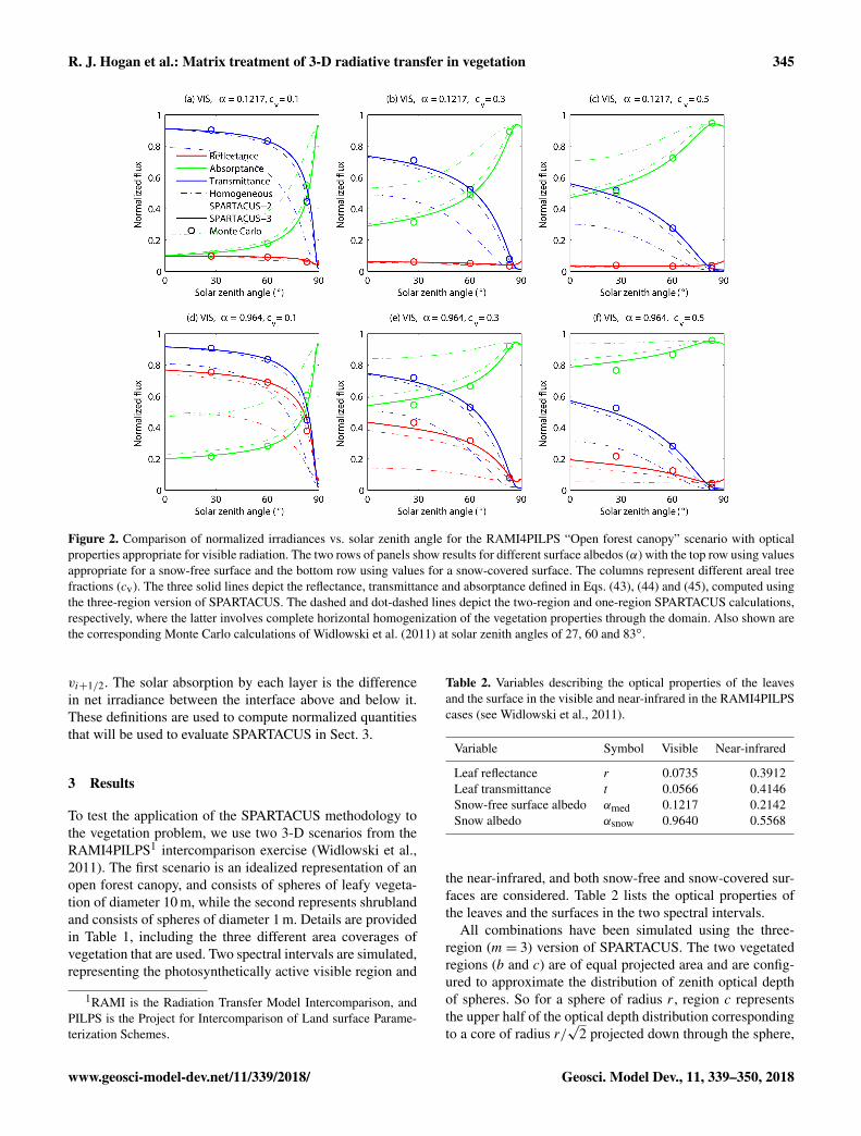
Figure 2. Comparison of normalized irradiances vs. solar zenith angle for the RAMI4PILPS “Open forest canopy” scenario with opticalproperties appropriate for visible radiation. The two rows of panels show results for different surface albedos (α) with the top row using valuesappropriate for a snow-free surface and the bottom row using values for a snow-covered surface. The columns represent different areal treefractions (cv). The three solid lines depict the reflectance, transmittance and absorptance defined in Eqs. (43), (44) and (45), computed usingthe three-region version of SPARTACUS. The dashed and dot-dashed lines depict the two-region and one-region SPARTACUS calculations,respectively, where the latter involves complete horizontal homogenization of the vegetation properties through the domain. Also shown arethe corresponding Monte Carlo calculations of Widlowski et al. (2011) at solar zenith angles of 27, 60 and 83◦.

vi+1/2. The solar absorption by each layer is the differencein net irradiance between the interface above and below it.These definitions are used to compute normalized quantitiesthat will be used to evaluate SPARTACUS in Sect. 3.

3 Results

To test the application of the SPARTACUS methodology tothe vegetation problem, we use two 3-D scenarios from theRAMI4PILPS1 intercomparison exercise (Widlowski et al.,2011). The first scenario is an idealized representation of anopen forest canopy, and consists of spheres of leafy vegeta-tion of diameter 10 m, while the second represents shrublandand consists of spheres of diameter 1 m. Details are providedin Table 1, including the three different area coverages ofvegetation that are used. Two spectral intervals are simulated,representing the photosynthetically active visible region and

1RAMI is the Radiation Transfer Model Intercomparison, andPILPS is the Project for Intercomparison of Land surface Parame-terization Schemes.

Table 2. Variables describing the optical properties of the leavesand the surface in the visible and near-infrared in the RAMI4PILPScases (see Widlowski et al., 2011).

Variable Symbol Visible Near-infrared

Leaf reflectance r 0.0735 0.3912Leaf transmittance t 0.0566 0.4146Snow-free surface albedo αmed 0.1217 0.2142Snow albedo αsnow 0.9640 0.5568

the near-infrared, and both snow-free and snow-covered sur-faces are considered. Table 2 lists the optical properties ofthe leaves and the surfaces in the two spectral intervals.

All combinations have been simulated using the three-region (m= 3) version of SPARTACUS. The two vegetatedregions (b and c) are of equal projected area and are config-ured to approximate the distribution of zenith optical depthof spheres. So for a sphere of radius r , region c representsthe upper half of the optical depth distribution correspondingto a core of radius r/

√2 projected down through the sphere,



Figure 3. As Fig. 2 but with optical properties appropriate for near-infrared radiation.

Figure 4. As Fig. 2 but for the RAMI4PILPS “Shrubland” scenario.



Figure 5. As Fig. 4 but with optical properties appropriate for near-infrared radiation.

which contains 1− 2−3/2, or 65 %, of its volume. Likewise,region b represents the lower half of the distribution corre-sponding to the remaining shell, and this contains 2−3/2, or35 %, of the volume of the sphere. Therefore, if the meanoptical depth of the sphere is δ, the mean optical depths ofregions b and c are 0.7δ and 1.3δ, respectively.

Figure 2 shows the results for the open forest canopyin the visible part of the spectrum while Fig. 3 shows thesame but for the near-infrared. The corresponding results forthe shrubland scenario are shown Figs. 4 and 5. Using thedomain-mean irradiances defined in Sect. 2.7, the quantitiesshown are reflectance R, transmittance T and absorptanceA:

R = u1/2/d1/2, (43)T = dn+1/2/d1/2, (44)A=

(d1/2− u1/2− dn+1/2+ un+1/2

)/d1/2. (45)

It can be seen that the three-region version of SPARTACUScompares well to Monte Carlo, including all four combina-tions of high- and low-reflectance leaves over a high- or low-reflectance surface. In total we have 72 points of comparisonwith Monte Carlo calculations: two scenarios, two spectralintervals, two surface types, three vegetation covers and threesolar zenith angles. Treating the Monte Carlo as “truth”, wecompute that the root-mean-squared error in R, T and A is0.020, 0.038 and 0.033, respectively. Probably the worse per-formance occurs for low solar zenith angle in Fig. 2f (corre-

sponding to visible radiation illuminating a scene with a treecover of 0.5 over snow): A is overestimated by around 0.05,suggesting that a little too much reflected sunlight from thesnow enters the tree crowns and is absorbed.

We next investigate how the results are degraded whenusing a more approximate description of the scene. Eachpanel of Figs. 2–5 includes two further lines. The “homo-geneous” calculation uses the same SPARTACUS code butwith only one region, treating the canopy as a single hori-zontally homogeneous layer with the same leaf area index.This is essentially the same as the Sellers (1985) assump-tion and indeed with a single region the matrix-exponentialmethod yields the same result as the Meador and Weaver(1980) solution. We see immediately that when the leavesare not clumped into trees but rather distributed uniformly,their exposure to incoming radiation is maximized and theirabsorptance is overestimated by up to 0.3. Conversely, boththe reflectance and transmittance of the scene are underesti-mated, with the largest error in reflectance for overhead sunand a snow-covered surface (Fig. 2e).

The two-region SPARTACUS calculation shown inFigs. 2–5 treats individual trees as horizontally homogeneouscylinders, thereby neglecting the variation in zenith opticaldepth of the spherical trees simulated by the Monte Carlocalculations. The results are much better than those with justa single region, and virtually the same as the three-region



calculation in the near infrared, but absorption still tends tobe overestimated in the visible. An analogous bias occurs incloudy radiative transfer calculations in which the internalvariability of clouds is neglected, which led to the proposalof Shonk and Hogan (2008) to use three regions to representa partially cloudy scene. The success of the three-region ap-proach suggests that it is also useful for vegetation. Havingsaid this, the uncertainty in computing radiative transfer thevegetation canopies of weather and climate models is typi-cally dominated by uncertainties in leaf area index. There-fore, for many applications the two-region calculation wouldbe adequate. Since the computational cost of SPARTACUS isdominated by the matrix exponential calculation, whose costis approximately proportional tom3, we would expect a two-region SPARTACUS calculation to be at least 3 times fasterthan a three-region calculation.

4 Discussion and conclusions

This paper has demonstrated the potential for the interactionof solar radiation and complex vegetation canopies to be rep-resented via an explicit description of the geometry, buildingon the SPARTACUS algorithm for representing the 3-D ra-diative effects of clouds (Hogan et al., 2016). The two-streamequations are written down for the tree crown and the gapsbetween them, but with additional terms for the horizontalexchange of radiation between regions. The equations aresolved exactly using the matrix exponential method. Multiplelayers are possible, although we have simplified the originalSPARTACUS algorithm by assuming maximum overlap be-tween the regions in each layer, rather than the arbitrary over-lap considered by Hogan et al. (2016). Comparison againstMonte Carlo calculations from the RAMI4PILPS intercom-parison exercise indicates that canopy reflectance, transmit-tance and absorptance are computed significantly more ac-curately than a number of state-of-the-art models assessedby Loew et al. (2014).

An advantage of the SPARTACUS approach is that in ad-dition to LAI, only a handful of physiographic variables arerequired to describe the geometry of the vegetation, such asthe vegetation height, coverage, and the diameter of typicaltree crowns. Global estimates of the first two are now avail-able from satellites (e.g. Simard et al., 2011; Hansen et al.,2003).

Although the testing scenarios used in this papers weresimple homogeneous spheres with no woody material, themethod described has the capability to represent more com-plex geometries. Horizontal variations in leaf density or treecrowns with different properties may be represented via twoor more vegetated regions with distinct optical properties.This paper considered a two-layer description of the vegeta-tion, with a single canopy layer overlying a sub-canopy layer,but the equations can easily be applied to a multi-layer de-scription of the canopy, for example to compute the verticalprofile of absorbed photosynthetically active radiation. Theoptical effects of tree trunks may also be incorporated. More-over, the good performance with solar radiation suggests thatthe thermal-infrared version of SPARTACUS (Schäfer et al.,2016) could also be adapted to the vegetation problem.

A further possible extension to SPARTACUS would be touse it for remote sensing; in addition to the possibility ofmore accurate LAI retrievals via explicit treatment of 3-Dradiative effects, this would provide a consistent frameworkfor both remote sensing and weather/climate modelling. Thechallenge would be to adapt SPARTACUS to compute solarradiances rather than irradiances, which adds an extra degreeof geometrical complexity. For example, trees cast shadowson the ground, but the extent to which shadows are visibleto a satellite depends on the sensor zenith angle and the az-imuthal separation of the sensor and the Sun.

Code availability. A MATLAB implementation of the algo-rithm is freely available from http://www.met.reading.ac.uk/clouds/spartacus and Zenodo (https://doi.org/10.5281/zenodo.1100534,Hogan, 2017). It was used to produce Figs. 2–5. Work is in progressto implement the algorithm in the “ecRad” atmospheric radiationscheme (Hogan and Bozzo, 2016).


http://www.met.reading.ac.uk/clouds/spartacus

http://www.met.reading.ac.uk/clouds/spartacus

https://doi.org/10.5281/zenodo.1100534


Appendix A: Faster treatment of clear layers

The main role of the sub-canopy layer is to represent howmuch of the sunlight passing down between the trees is re-flected back up into the base of a tree crown, i.e. the off-diagonal elements of An−1/2 and Dn−1/2. Since the matrixexponential accounts for most of the cost of the scheme, ifwe can accelerate or approximate the treatment of the sub-canopy layer in a way that avoids the full matrix-exponentialcalculation in this layer then we can almost halve the over-all computational cost. This is only possible if we assumethat the sub-canopy layer contains no absorbers or scatterers(σ = σ0 = 0), i.e. tree trunks and understory vegetation areneglected.

There are two extreme scenarios that lead to An−1/2 andDn−1/2 having trivial forms. For shrubs with a very shallowsub-canopy layer, the lateral transport between the regions ofthis layer is zero, leading to albedo matrices at the interfacebetween the canopy and sub-canopy layer being equal to thevalues at the surface given by Eqs. (35) and (36). For a verydeep sub-canopy layer, the radiation field beneath the canopyis randomized horizontally, leading to the diffuse albedo hav-ing the form

An−1/2 '

ca ca ca

cb cb cb

cc cc cc

αdiff, (A1)

where αdiff is the domain-averaged surface albedo to diffuseradiation. The direct albedo Dn−1/2 has a similar form.

For sub-canopy layers with a depth between these two ex-tremes, we seek to optimize the calculation of the matrix ex-ponential. The lack of scattering means that the 02, 03 and04 sub-matrices contain only zeros, and 0 becomes block-diagonal. This enables the exponential of a 3m× 3m matrixto be replaced by three m×m matrix-exponential calcula-tions, only two of which are needed: E0 = exp(001z) andEvv = exp(011z). Since there is no scattering in the sub-canopy layer, the matrices R, S+ and S− contain only zeros.Therefore, Eq. (27) simplifies to T= Evv , and Eqs. (33) and(34) simplify to

An−1/2 = TnAn+1/2Tn, (A2)Dn−1/2 = TnDn+1/2E0n. (A3)

Moreover, by approximating the extinction coefficients aszero, we see from Eqs. (3) and (4) that 00 and 01 have sim-pler forms whose matrix exponentials can be derived analyt-ically. In the m= 2 case these matrices have the form

0′ =

(−a b

a −b

), (A4)

for which the matrix exponential is given by Putzer’s algo-rithm as

exp(0′1z

)= I+

1− e−(a+b)1z

a+ b0′. (A5)

Likewise in the m= 3 case these matrices have the form

0′ =

−a b 0a −b− c c

0 c −c

, (A6)

for which the matrix exponential may be computed by thediagonalization method as

exp(0′1z

)= V

eλ11z

eλ21z

1

V−1, (A7)

where the two non-zero eigenvalues are

λ=−(a+ b+ 2c)/2± (a2+ b2+ 4c2

+ 2ab− 4ac)1/2/2, (A8)

and the matrix of eigenvectors is

V=

b/(a+ λ1) b/(a+ λ2) b/a

1 1 1c/(c+ λ1) c/(c+ λ2) 1

. (A9)



The Supplement related to this article is available onlineat https://doi.org/10.5194/gmd-11-339-2018-supplement.

Competing interests. The authors declare that they have no conflictof interest.

Acknowledgements. We thank Jean-Luc Widlowski for providingthe Monte Carlo results. Tristan Quaife’s contribution was fundedby the UK National Centre for Earth Observation. Renato Braghierewas supported by a scholarship from the Brazilian “Science withoutBorders” Program (grant number 9549-13-7), financed by CAPES,the Brazilian Federal Agency for Support and Evaluation ofGraduate Education within the Ministry of Education of Brazil.

Edited by: Jatin KalaReviewed by: two anonymous referees

References

Best, M. J., Pryor, M., Clark, D. B., Rooney, G. G., Essery, R. L.H., Ménard, C. B., Edwards, J. M., Hendry, M. A., Porson, A.,Gedney, N., Mercado, L. M., Sitch, S., Blyth, E., Boucher, O.,Cox, P. M., Grimmond, C. S. B., and Harding, R. J.: The JointUK Land Environment Simulator (JULES), model description –Part 1: Energy and water fluxes, Geosci. Model Dev., 4, 677–699,https://doi.org/10.5194/gmd-4-677-2011, 2011.

Hansen, M., DeFries, R. S., Townshend, J. R. G., Carroll, M., Dim-iceli, C., and Sohlberg, R. A.: Global percent tree cover at a spa-tial resolution of 500 meters: first results of the MODIS vegeta-tion continuous fields algorithm, Earth Interact., 7, 1–15, 2003.

Higham, N. J.: The scalingand squaring method for the Matrix Ex-ponential revisited, SIAM J. Matrix Anal. A., 26, 1179–1193,2005.

Hogan, R. J.: SPARTACUS Vegetation 1.1: Matlab imple-mentation of a matrix method to compute 3D radia-tive transfer in vegetation canopies (Version 1.1), Zenodo,https://doi.org/10.5281/zenodo.1100535, 2017.

Hogan, R. J. and Bozzo, A.: ECRAD: A New Radiation Scheme forthe IFS, ECMWF Technical Memorandum 787, 33 pp., 2016.

Hogan, R. J. and Shonk, J. K. P.: Incorporating the effects of 3Dradiative transfer in the presence of clouds into two-stream mul-tilayer radiation schemes, J. Atmos. Sci., 70, 708–724, 2013.

Hogan, R. J., Schäfer, S. A. K., Klinger, C., Chiu, J.-C., andMayer, B.: Representing 3D cloud-radiation effects in two-stream schemes: 2. Matrix formulation and broadband evalua-tion, J. Geophys. Res.-Atmos., 121, 8583–8599, 2016.

Jensen, M. P., Vogelmann, A. M., Collins, W. D., Zhang, G. J., andLuke, E. P.: Investigation of regional and seasonal variations inmarine boundary layer cloud properties from MODIS observa-tions, J. Climate, 21, 4955–4973, 2008.

Lacis, A. A. and Hansen, J. E.: A parameterization for the absorp-tion of solar radiation in the Earth’s atmosphere, J. Atmos. Sci.,31, 118–133, 1974.

Loew, A., van Bodegom, P. M., Widlowski, J.-L., Otto, J., Quaife,T., Pinty, B., and Raddatz, T.: Do we (need to) care about canopyradiation schemes in DGVMs? Caveats and potential impacts,Biogeosciences, 11, 1873–1897, https://doi.org/10.5194/bg-11-1873-2014, 2014.

Meador, W. E. and Weaver, W. R.: Two-stream approximations toradiative transefer in planetary atmospheres: a unified descriptionof existing methods and a new improvement, J. Atmos. Sci., 37,630–643, 1980.

Morcrette, C. J.: Improvements to a prognostic cloud schemethrough changes to its cloud erosion parametrization, Atmos. Sci.Lett., 13, 95–102, 2012.

Ni-Meister, W., Yang, W., and Kiang, N. Y.: A clumped-foliagecanopy radiative transfer model for a global dynamic terrestrialecosystem model. 1: Theory, Agr. Forest Meteorol., 150, 881–894, 2010.

Pinty, B., Lavergne, T., Dickinson, R. E., Widlowski, J.-L., Go-bron, N., and Verstraete, M. M.: Simplifying the interactionof land surfaces with radiation for relating remote sensingproducts to climate models, J. Geophys. Res., 111, D02116,https://doi.org/10.1029/2005JD005952, 2006.

Putz, F. E., Parker, G. G., and Archibald, R. M.: Mechanical abra-sion and intercrown spacing, Am. Midl. Nat., 112, 24–28, 1984.

Schäfer, S. A. K., Hogan, R. J., Klinger, C., and Mayer, B.: Rep-resenting 3D cloud-radiation effects in two-stream schemes: 1.Longwave considerations and effective cloud edge length, J. At-mos. Sci., 121, 8567–8582, 2016.

Sellers, P. J.: Canopyreflectance, photosynthesis and transpiration,Int. J. Remote Sens., 6, 1335–1372, 1985.

Shonk, J. K. P. and Hogan, R. J.: Tripleclouds: an efficient methodfor representing horizontal cloud inhomogeneity in 1D radiationschemes by using three regions at each height, J. Climate, 21,2352–2370, 2008.

Simard, M., Pinto, N., Fisher, J. B., and Baccini, A.: Mapping forestcanopy height globally with spaceborne lidar, J. Geophys. Res.-Biogeo., 116, G04021, https://doi.org/10.1029/2011JG001708,2011.

Tiedtke, M.: Anextension of cloud-radiation parameterization in theECMWF model: the representation of subgrid-scale variations ofoptical depth, Mon. Weather Rev., 124, 745–750, 1996.

Viterbo, P. and Betts, A. K.: Impact on ECMWF forecasts ofchanges to the albedo of the boreal forests in the presence ofsnow, J. Geophys. Res., 104, 27803–27810, 1999.

Waterman, P. C.: Matrix-exponential description of radiative trans-fer, J. Opt. Soc. Am., 71, 410–422, 1981.

Widlowski, J.-L., Pinty, B., Clerici, M., Dai, Y., De Kauwe, M.,de Ridder, K., Kallel, A., Kobayashi, H., Lavergne, T., Ni-Meister, W., Olchev, A., Quaife, T., Wang, S., Yang, W.,Yang, Y., and Yuan, H.: RAMI4PILPS: an intercompari-son of formulations for the partitioning of solar radiation inland surface models, J. Geophys. Res.-Biogeo., 116, G02019,https://doi.org/10.1029/2010JG001511, 2011.


https://doi.org/10.5194/gmd-11-339-2018-supplement

https://doi.org/10.5194/gmd-4-677-2011

https://doi.org/10.5281/zenodo.1100535

https://doi.org/10.5194/bg-11-1873-2014

https://doi.org/10.5194/bg-11-1873-2014

https://doi.org/10.1029/2005JD005952

https://doi.org/10.1029/2011JG001708

https://doi.org/10.1029/2010JG001511

fast matrix treatment of 3-d radiative transfer in

Documents