Fast Incremental Learning for Off-Road Robot Navigation

___________________________________________________

Artem Provodin

New York University

New York NY 10003

Liila Torabi Net-Scale Technologies

Morganville NJ 07751

Beat Flepp

NVIDIA Corp Holmdel NJ 07733

L. D. Jackel

North C Technologies

Holmdel NJ 07733

Yann LeCun

New York University New York NY10003

Urs Muller

NVIDIA Corp

Holmdel NJ 07733

Michael Sergio

Net-Scale Technologies Morganville NJ 07751

Jure Žbontar

New York University

New York NY 10003

Abstract

A promising approach to autonomous driving is machine learning. In such systems, training datasets are created that capture the sensory input to a vehicle as well as the desired

response. A disadvantage of using a learned navigation system is that the learning process

itself may require a huge number of training examples and a large amount of computing.

To avoid the need to collect a large training set of driving examples, we describe a system

that takes advantage of the huge number of training examples provided by ImageNet, but is able to adapt quickly using a small training set for the specific driving environment.

1 Introduction

Despite remarkable advances in autonomous vehicles, off-road autonomous ground navigation remains an

unsolved challenge. The difficulty of the task arises from the enormous variability that an Unmanned Ground

Vehicle confronts when it leaves the relatively well characterized domain of the road. While it may be possible to create a rule-based system that codifies all situations that might be presented to the vehicle, such approaches

are brittle, and tend to fail when new environments are encountered.

A more promising approach to autonomous driving is machine learning. In such systems, training datasets are

created that capture the sensory input to a vehicle as well as the desired response. These responses may be provided by a human driver who initially teleoperates the vehicle, or may be gleaned from the vehicle’s prior

driving experiences.

Page 2 of 14

A number of systems have been described that learn drivable vs non-drivable terrain using handcrafted features

based on color or texture (see, for example, Sofman 2010). In recent years, Convolution Neural Networks

[ConvNets] (LeCun et al 1989), in which the features are learned rather than handcrafted, have been shown to be the most accurate in numerous image recognition tasks (see, for example, Krizhevsky et al 2012).

A disadvantage of using a learned system is that the learning process itself may require a huge number of

training examples and a large amount of computing. As an illustration, the most accurate networks used in the

ImageNet competitions (ILSVRC 2014) train on over one million examples and often require days of training

on powerful processor clusters. While such expensive training may be fine for some applications, it is unacceptable for systems that have to adapt quickly and only have limited training data. Here we describe a

system that takes advantage of the huge number of training examples provided by ImageNet, but is able to

adapt quickly using a small training set.

2 System Overview

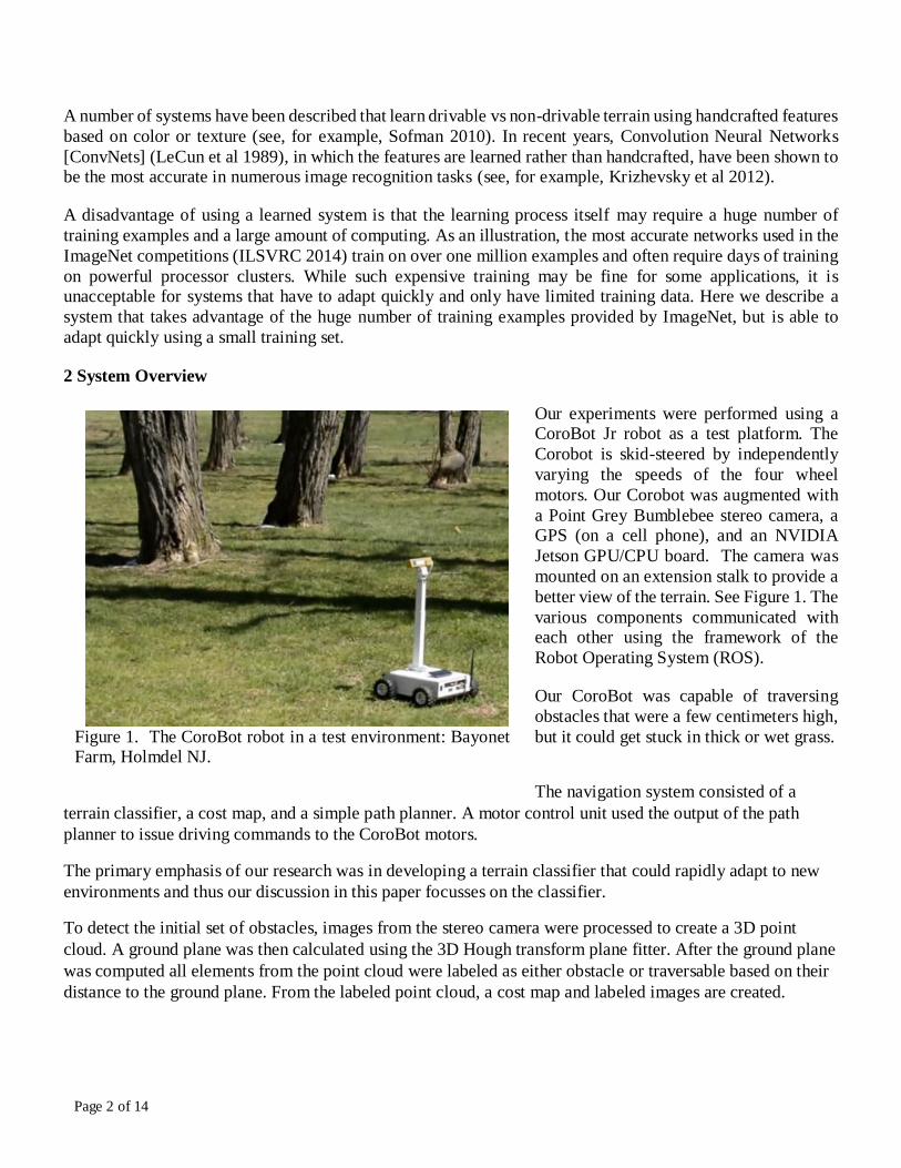
Our experiments were performed using a CoroBot Jr robot as a test platform. The

Corobot is skid-steered by independently

varying the speeds of the four wheel

motors. Our Corobot was augmented with

a Point Grey Bumblebee stereo camera, a GPS (on a cell phone), and an NVIDIA

Jetson GPU/CPU board. The camera was

mounted on an extension stalk to provide a

better view of the terrain. See Figure 1. The

various components communicated with each other using the framework of the

Robot Operating System (ROS).

Our CoroBot was capable of traversing

obstacles that were a few centimeters high,

but it could get stuck in thick or wet grass.

The navigation system consisted of a

terrain classifier, a cost map, and a simple path planner. A motor control unit used the output of the path

planner to issue driving commands to the CoroBot motors.

The primary emphasis of our research was in developing a terrain classifier that could rapidly adapt to new

environments and thus our discussion in this paper focusses on the classifier.

To detect the initial set of obstacles, images from the stereo camera were processed to create a 3D point

cloud. A ground plane was then calculated using the 3D Hough transform plane fitter. After the ground plane

was computed all elements from the point cloud were labeled as either obstacle or traversable based on their

distance to the ground plane. From the labeled point cloud, a cost map and labeled images are created.

Figure 1. The CoroBot robot in a test environment: Bayonet Farm, Holmdel NJ.

Page 3 of 14

The navigation system calculates the optimal driving direction based on the cost map and the goal position.

The trajectory planner incorporates the distance to an obstacle to calculate the drive direction so that the

CoroBot avoids obstacles.

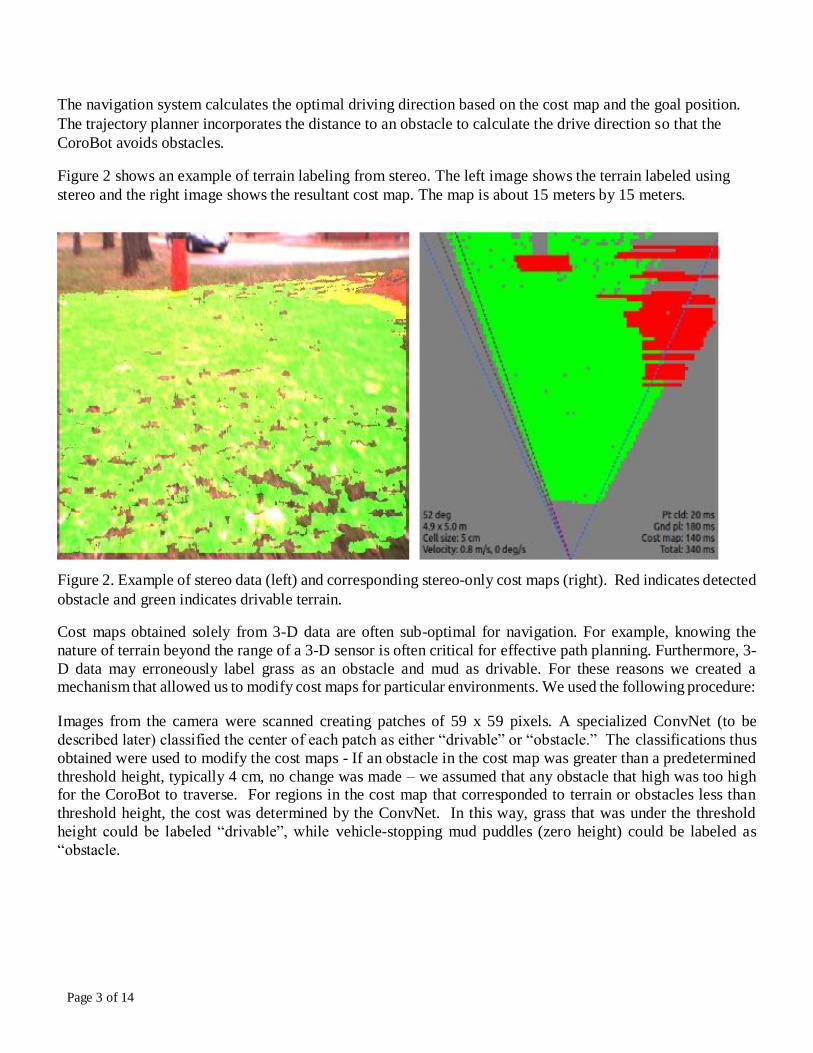
Figure 2 shows an example of terrain labeling from stereo. The left image shows the terrain labeled using

stereo and the right image shows the resultant cost map. The map is about 15 meters by 15 meters.

Figure 2. Example of stereo data (left) and corresponding stereo-only cost maps (right). Red indicates detected

obstacle and green indicates drivable terrain.

Cost maps obtained solely from 3-D data are often sub-optimal for navigation. For example, knowing the

nature of terrain beyond the range of a 3-D sensor is often critical for effective path planning. Furthermore, 3-

D data may erroneously label grass as an obstacle and mud as drivable. For these reasons we created a mechanism that allowed us to modify cost maps for particular environments. We used the following procedure:

Images from the camera were scanned creating patches of 59 x 59 pixels. A specialized ConvNet (to be

described later) classified the center of each patch as either “drivable” or “obstacle.” The classifications thus

obtained were used to modify the cost maps - If an obstacle in the cost map was greater than a predetermined

threshold height, typically 4 cm, no change was made – we assumed that any obstacle that high was too high for the CoroBot to traverse. For regions in the cost map that corresponded to terrain or obstacles less than

threshold height, the cost was determined by the ConvNet. In this way, grass that was under the threshold

height could be labeled “drivable”, while vehicle-stopping mud puddles (zero height) could be labeled as

“obstacle.

Page 4 of 14

3 Training the ConvNets

In order to build accurate classifiers, ConvNets with many weights are required. Training these weights

requires many labeled training examples. Obtaining an adequate number of training examples using just imagery for the CoroBot camera was not practical since that would have required extensive hand-labelling.

Fortunately, the ImageNet database provided an attractive and effective alternative. ImageNet includes about

1,000,000 images that are divided into 1000 labeled classes. In the last few years there has been tremendous

progress in creating ConvNets that keep advancing the accuracy of classifying the ImageNet test data. We

have been able to piggyback on this progress.

Our systems start with ConvNets that have been trained on ImageNet. We then preserve some of the initial

layers of these trained ConvNets for use as feature extractors for our navigation task. A separate navigation

training set is then created using the features extracted from the 59 x 59 patches taken from images in our

driving environment. We used patches, instead of just single labeled pixels because we hypothesized that

having “context” around the pixel in question would improve classification.

A subset of these patches were labeled by a human that identifying areas that might be misclassified by stereo.

Next, a single-layer perceptron was trained using these feature/label pairs, i.e. each training example pair

contains a feature vector obtained from the feature extractor applied to a patch and a label for that patch which

was either “drivable” or “not-drivable”. After this training, which can be done in a few seconds, a new

classifier was obtained that combined ImageNet-derived feature extraction and customized terrain classification. This new classifier was then used to label terrain in new images without using stereo.

The above strategy is an example of “transfer learning” in which a system designed for one task (in the case

ImageNet classification) is repurposed to perform a different task (terrain classification).

3.1 ImageNet Learning

The architecture of our ConvNet is shown in Figure 3. During training, the input to our ConvNet has 3

input image RGB planes, each 119 x 119 pixels taken from the ImageNet database.

● The first layer applies 64 filters, each 8x8 pixels, to the input. The first layer used a stride of 4x4, and

the maps produced by it are therefore 28x28. This convolutional step is then followed by a

thresholding operation, and a max pooling function, which pools regions of size 2x2, and uses a stride

of 2x2. The result of that operation is a 64x14x14 array, which represents a 14x14 map of 64-

dimensional feature vectors. The receptive field in the input image of each unit at this stage is 8x8.

● The second layer (conv+pooling) is very much analogous to the first, except that now the 64-dim

feature maps are projected into 96-dim maps (5x5 size filters). The result of the complete layer

(conv+pooling) is a 96x5x5 array.

● In the last stage, the 5x5 array of 96-dimensional feature vectors is flattened into a 2400-dimensional

vector, which is fed to a 2-layer classifier with 1536 hidden units, and 1000 output classes.

Page 5 of 14

Figure 3. ConvNet feature extractor structure

The loss function is set to negative log likelihood criterion.

Page 6 of 14

3.1.1 Details of Training Process

To speed network training, an NVIDIA GTX Titan GPU graphics card was used. To parallelize the training,

~15,000 batches of 64 119 x 119 RGB scaled ImageNet images were prepared as training input along with

their ImageNet classification labels. The only pre-processing was subtracting the mean RGB value,

computed on the first (shuffled) 10000 images, from each pixel.

We train the network using stochastic gradient descent with momentum set to 0.08. The learning rate is

calculated according to the formula 0.05 ∗ √𝑏𝑎𝑡𝑐ℎ 𝑠𝑖𝑧𝑒/√128 and multiplied by 0.96 each iteration, which

consist of 4 datasets described in the next section. On a system equipped with an NVIDIA GTX Titan

GPU, training a single net took one week.

3.1.2 Data Set Augmentation

Augmenting the data set by repeatedly transforming the training examples is a commonly employed trick to

reduce the network’s generalization error. The transformations are applied at training time and do not affect

the runtime performance.

We scaled the ImageNet images to 128 x 128 pixels from which we extracted training patches size 119 x

119. Then we randomly rotated, scaled and sheared the training patches according to the following rules:

● Flip: horizontally flip 25% of the examples, vertically flip 25%, both flip 25%, no change 25%.

● Scale: choose a random scale factor in the range of 0.83 to 1.2.

● Rotate: choose a random rotation angle in the range of -30 to +30 degrees.

● Shift horizontal and vertical direction (-5 to 5 pixels) and crop to 119 x 119.

Thus, the training data comprised 4 subsets, each obtained from the ImageNet initial data.

3.2 Terrain Classification Task

Our objective here was not to create the very best ImageNet classifier, but rather to learn feature vectors (the

output of the penultimate layer in our network) which could then be used for fast training of a linear network

that uses navigation sensor input coupled with labeled terrain classes as training examples. With the feature

extraction layer weights frozen, and the fully-connected neural network with one or more hidden layers

trained using these feature/label pairs appended, we created a classifier to be used during navigation.

Our network was designed to train on regions of an image where the terrain type was known, say from stereo

data, or by labeling by a human operator. The networks would then classify regions that were not known,

usually from an entirely new frame, but from the same environment.

Images for navigation training were labeled by having a human operator label representative obstacles in the

Page 7 of 14

environment. The patches, which were 59 x 59 pixels, were labeled by the class of the center pixel, i.e. each

training example contains a feature vector obtained from the feature extractor applied to a patch and the label

for that patch “drivable” or “obstacle”.

4 Implementation Details

4.1 Sensors

To process the camera images, we added the Robot Operating System (ROS) image pipeline stack in order to

integrate better with the open source ROS environment and to eliminate the dependency of the external and

proprietary stereo processing library. This ROS stack provided a set of modules for stereo processing,

visualization and camera calibration. The stereo image processing took the raw images from our custom

written camera driver for Bumblebee cameras, and performed image rectification (distortion correction and

alignment) and color processing for both the left and the right camera. The ROS image pipeline stack

performed the required process on the both raw images and finally created the point cloud.

4.2 Classification

Torch7 (a scientific computing framework with wide support for machine learning algorithms) was used in

the current project because it provided an easy and modular way to build and train simple or complex neural

networks. As a part of the navigation system, the classification algorithm was integrated into the ROS

environment via a special library that converted images to the Torch tensor representation, facilitating

processing by the ConvNet. The ConvNet returned classified labels for each pixel.

The classifier could be trained either in real time or after different images were gathered and labelled by a

human. Classifier training could be done on an external computer, i.e. the laptop that is used to control the

robot in the field. Training could be accomplished in a few seconds using a GPU enabled laptop. After

training, the new classifier was uploaded on to the robot.

5 Results and Discussion

5.1 Off-line Learning From a Human Teacher

A human teacher was used to label terrain that might be misclassified if we relied solely on stereo. The

human labeled representative terrain in one or a few images and we then used those labels for many images

in the same environment. Several images were chosen from different scenes as shown in Figure 4. Green

and Red tints indicate human labeled obstacles and drivable terrain (on the left) and the corresponding

classification result (on the right). In the upper images, flat snow-covered ground is classified as an obstacle,

while pavement is classified as drivable.

In the lower images of Figure 4 regions with small plants were classified as “drivable” while regions with

bushes and trees were classified as “obstacles”. While the results are not perfect, they clearly show as

“drivable” the terrain that is interspersed with small plants, regions that using stereo alone would have

classified as having obstacles.

Page 8 of 14

Figure 4: Examples of learning from hand-labeled region (left column) and classifications provided

by our system (right column). Red indicates obstacles and green indicates drivable terrain.

Figure 5 shows the effect of adding more human-supplied training labels. The left image in the

upper row shows the few pixels that were hand labeled as red and green streaks. The right image

shows the classification of the entire image based on these sparse labels. In the lower row, more

pixels were labeled (left image) resulting in a more precise labeling of the remaining pixels (right

in image).

Page 9 of 14

Figure 5. The effect of adding more human-supplied training labels. Labeled areas are shown as overlays in

the left column and the resulting classifications are shown in the right column. Red indicates obstacles and

green indicates drivable terrain. Adding more labels (lower row), gives a more precise classification than

with fewer labels (upper row).

5.2 Navigation

The ConvNet could be trained in real time on images from the current environment in which a small number

of representative images patches were hand labeled. As noted previously, the patches chosen for hand

labeling were ones from regions that would be improperly classified by stereo alone. Labels from the

ConvNet and the point cloud were then combined in a cost map using the following method:

First, stereo was used to identify as obstacles objects that extended above the ground plane by more than an

operator set threshold, typically 15 cm. For objects less than this threshold, the label obtained from the

Page 10 of 14

ConvNet was used for classification. In cases where stereo could not provide a height estimate, such as for

surfaces that lack sufficient features to measure disparity, we simply used the labels obtained from the

ConvNet.

Below we present results obtained by running the robot in various environments. Corresponding videos can

be found on line at

https://www.youtube.com/watch?v=zesKN_1i9VA https://www.youtube.com/watch?v=AXFupI_Nz8E https://www.youtube.com/watch?v=gDFQhFbX3oU

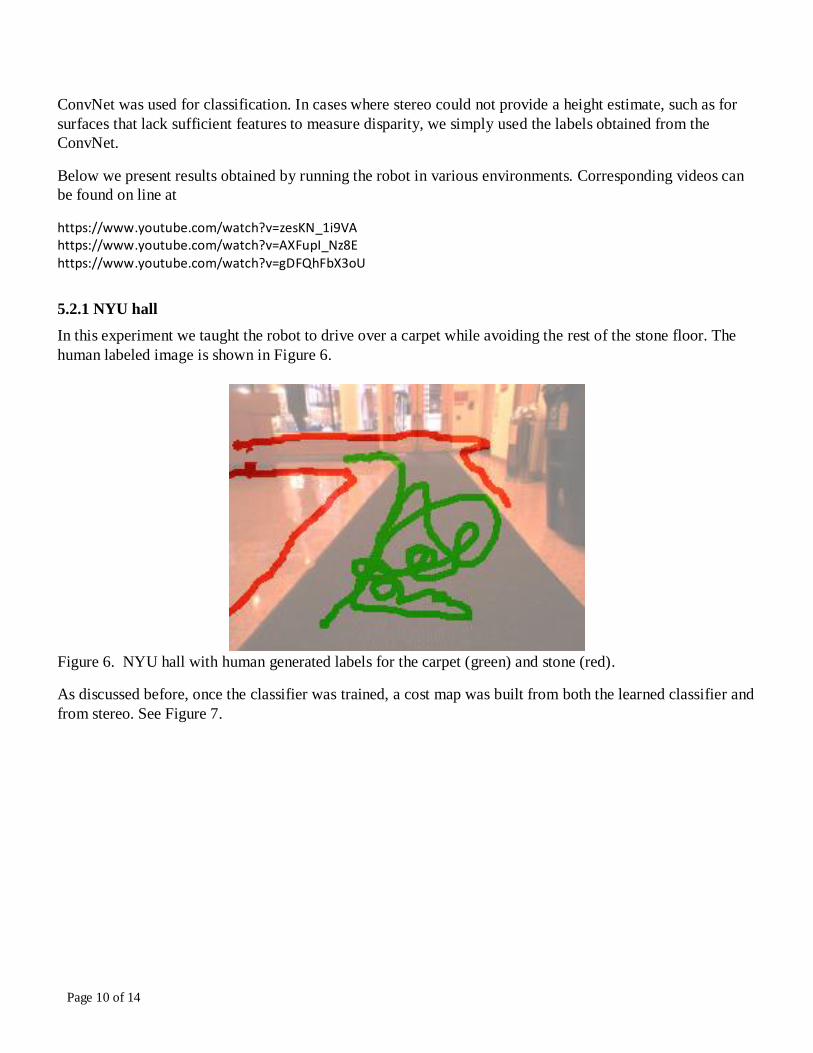
5.2.1 NYU hall

In this experiment we taught the robot to drive over a carpet while avoiding the rest of the stone floor. The

human labeled image is shown in Figure 6.

Figure 6. NYU hall with human generated labels for the carpet (green) and stone (red).

As discussed before, once the classifier was trained, a cost map was built from both the learned classifier and

from stereo. See Figure 7.

Page 11 of 14

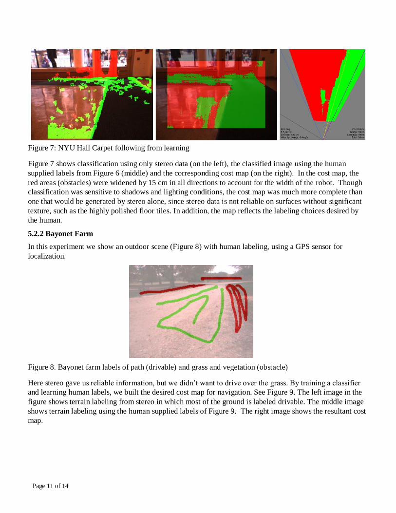
Figure 7: NYU Hall Carpet following from learning

Figure 7 shows classification using only stereo data (on the left), the classified image using the human

supplied labels from Figure 6 (middle) and the corresponding cost map (on the right). In the cost map, the

red areas (obstacles) were widened by 15 cm in all directions to account for the width of the robot. Though

classification was sensitive to shadows and lighting conditions, the cost map was much more complete than

one that would be generated by stereo alone, since stereo data is not reliable on surfaces without significant

texture, such as the highly polished floor tiles. In addition, the map reflects the labeling choices desired by

the human.

5.2.2 Bayonet Farm

In this experiment we show an outdoor scene (Figure 8) with human labeling, using a GPS sensor for

localization.

Figure 8. Bayonet farm labels of path (drivable) and grass and vegetation (obstacle)

Here stereo gave us reliable information, but we didn’t want to drive over the grass. By training a classifier

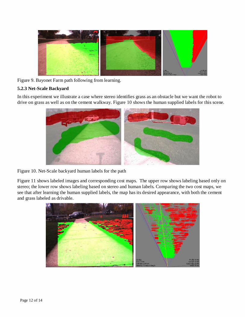
and learning human labels, we built the desired cost map for navigation. See Figure 9. The left image in the

figure shows terrain labeling from stereo in which most of the ground is labeled drivable. The middle image

shows terrain labeling using the human supplied labels of Figure 9. The right image shows the resultant cost

map.

Page 12 of 14

Figure 9. Bayonet Farm path following from learning.

5.2.3 Net-Scale Backyard

In this experiment we illustrate a case where stereo identifies grass as an obstacle but we want the robot to

drive on grass as well as on the cement walkway. Figure 10 shows the human supplied labels for this scene.

Figure 10. Net-Scale backyard human labels for the path

Figure 11 shows labeled images and corresponding cost maps. The upper row shows labeling based only on

stereo; the lower row shows labeling based on stereo and human labels. Comparing the two cost maps, we

see that after learning the human supplied labels, the map has its desired appearance, with both the cement

and grass labeled as drivable.

Page 13 of 14

Figure 11: Net-Scale backyard path.

6 Conclusion

We have shown that using the feature extractors obtained from previously trained ConvNets provides good

terrain classification, even though the original ConvNets were trained on a completely different corpus.

Training the single layer perceptrons that use the feature vectors extracted by the initial layers of the

ConvNets is sufficiently fast that the process provides a promising method for rapid adaptation while

navigating in diverse environments.

These results illustrate the feasibility of real-time tuning of autonomous robot navigation preferences,

creating a system that is highly customizable and adaptive.

Acknowledgement

This material is based upon work supported by the United States Army under Contract No. W56HZV-13-C-

0014.

Any opinions, findings and conclusions or recommendations expressed in this material are those of the

author(s) and do not necessarily reflect the views of the United States Army

References

ILSVRC 2014 http://image-net.org/challenges/LSVRC/2014/index

Krizhevsky, A., Sutskever, I., Hinton, G. E., (2012). ImageNet Classification with Deep Convolutional

Neural Networks. In: Pereira, F., Burges, C.J.C., Bottou. L., Weinberger, K.Q., editors. Advances in Neural

Information Processing Systems 25. Curran Associates, 1097–1105.

LeCun, Y., Boser, B., Denker, J. S., Henderson, D., Howard., R. E., Hubbard, W., and Jackel, L. D. (1989)

Backpropagation Applied to Handwritten Zip Code Recognition. Neural Computation 1:541-551.

Page 14 of 14

Sofman, B. (2010). Online Learning Techniques for Improving Robot Navigation in Unfamiliar Domains,

doctoral dissertation, tech report CMU RI-TR-10-43, Robotics Institute, Carnegie Mellon University.