Fast Imaging Trajectories:Non-Cartesian Sampling (2)

M229 Advanced Topics in MRI Holden H. Wu, Ph.D.

2018.05.08

Department of Radiological Sciences David Geffen School of Medicine at UCLA

Class Business

• Final project - Proposal due 5/11 Fri

can send us a draft to get feedback - Presentations:

6/7 Thu 9 am - 12 noon, and 6/8 Fri 3 pm - 6 pm

Outline

• Spiral Trajectory

• Non-Cartesian 3D Trajectories - 3D stack of radial - 3D radial (koosh ball) - 3D cones

• Non-Cartesian Image Reconstruction - Gridding reconstruction - Gradient measurement - Off-resonance correction (if time permits)

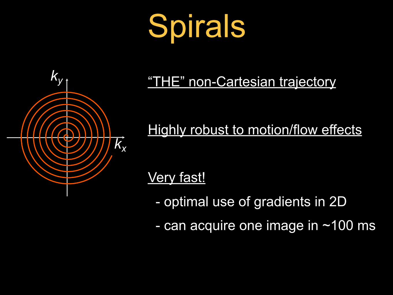
Spiralsky

kx

“THE” non-Cartesian trajectory

Highly robust to motion/flow effects

Very fast!

- optimal use of gradients in 2D

- can acquire one image in ~100 ms

Spirals: Sampling RequirementsN interleaves

2 kr,max = 1 / dx

dk = 1 / FOV

Design 1 interleaf

and rotate

Subject to HW limits

Spirals: Gradient Designk-space trajectory

Gradients vs. time Slew rate vs. time

k-space pos vs. time

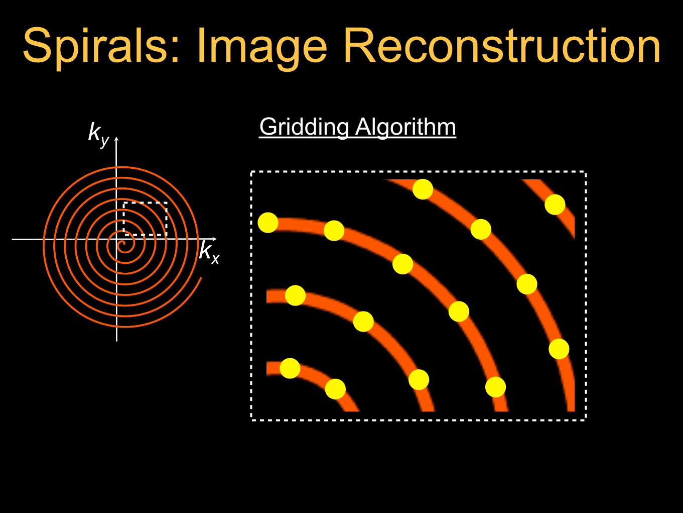
Spirals: Image Reconstructionky

kx

Gridding Algorithm

Spirals: Image Reconstructionky

kx

Gridding Algorithm

Spirals: Image Reconstructionky

kx

Gridding Algorithm

Follow with 2D Fourier Transform ...

Spirals: Gradient Delays

2 sample delay 1 sample delay calibrated

Spirals: Off-Resonance Effects

Nintlv = 8

Trd = 26.67 ms

Nintlv = 16

Trd = 13.41 ms

Nintlv = 48

Trd = 4.61 ms

Spirals: Practical Considerations

ky

kx

Trajectory design

Gradient waveform calibration

k-Space density compensation

Off-resonance correction

Fat suppression

Gridding reconstruction

applies to non-Cartesian MRI in general

Spirals: Real-Time Cardiac MRI

- Healthy volunteer; 1.5 T; 8-ch array - Golden-angle ordering - Spiral 2D GRE; 8-mm slice - Spatial resolution = 1.6 mm - SPIRiT recon with R = 2 - 40 cm, 1.6 mm - 250x250 matrix @ 6 fps - 12-fold reduction in #TRs (vs. 2DFT) - 8-TR sliding window display (16 fps)

Wu HH et al., ISMRM 2013, p3828

Spirals: 3D LGE MRI

courtesy of Joelle Barral & Juan Santos (HeartVista)

3D Spiral IR-GRE - 6-interleaf VD spiral - 7.5-ms readout - 90 x 90 x 11 matrix - outer volume suppr - water-only RF exc - TR = 15.48 ms - 8-HB BH scan

Reconstruction - SPIRiT (R = 2) - ~5-sec recon

1.5 T

Spirals: Pros and Consky

kx

Pros

- Very fast (up to single shot)

- Very short TE

- Robust to motion/flow effects

Cons

- May have mixed contrast

- Sensitive to gradient delays

- Sensitive to off-resonance effects

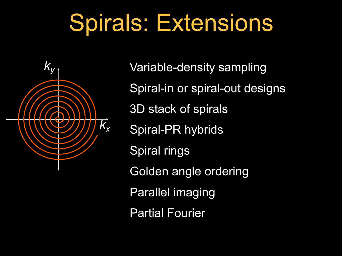
Spirals: Extensionsky

kx

Variable-density sampling

Spiral-in or spiral-out designs

3D stack of spirals

Spiral-PR hybrids

Spiral rings

Golden angle ordering

Parallel imaging

Partial Fourier

Spirals: Applicationsky

kx

Fast imaging and real-time imaging

- Cardiac MRI

- Functional MRI (fMRI)

- Dynamic contrast-enhanced MRI

- MR spectroscopic imaging

Improve motion/flow robustness

- Cardiac MRI

- Abdominal MRI

Non-Cartesian Samplingky

kx

2D Concentric Rings 2D Spiral2D Radial

ky

kx

ky

kx

and much more ...

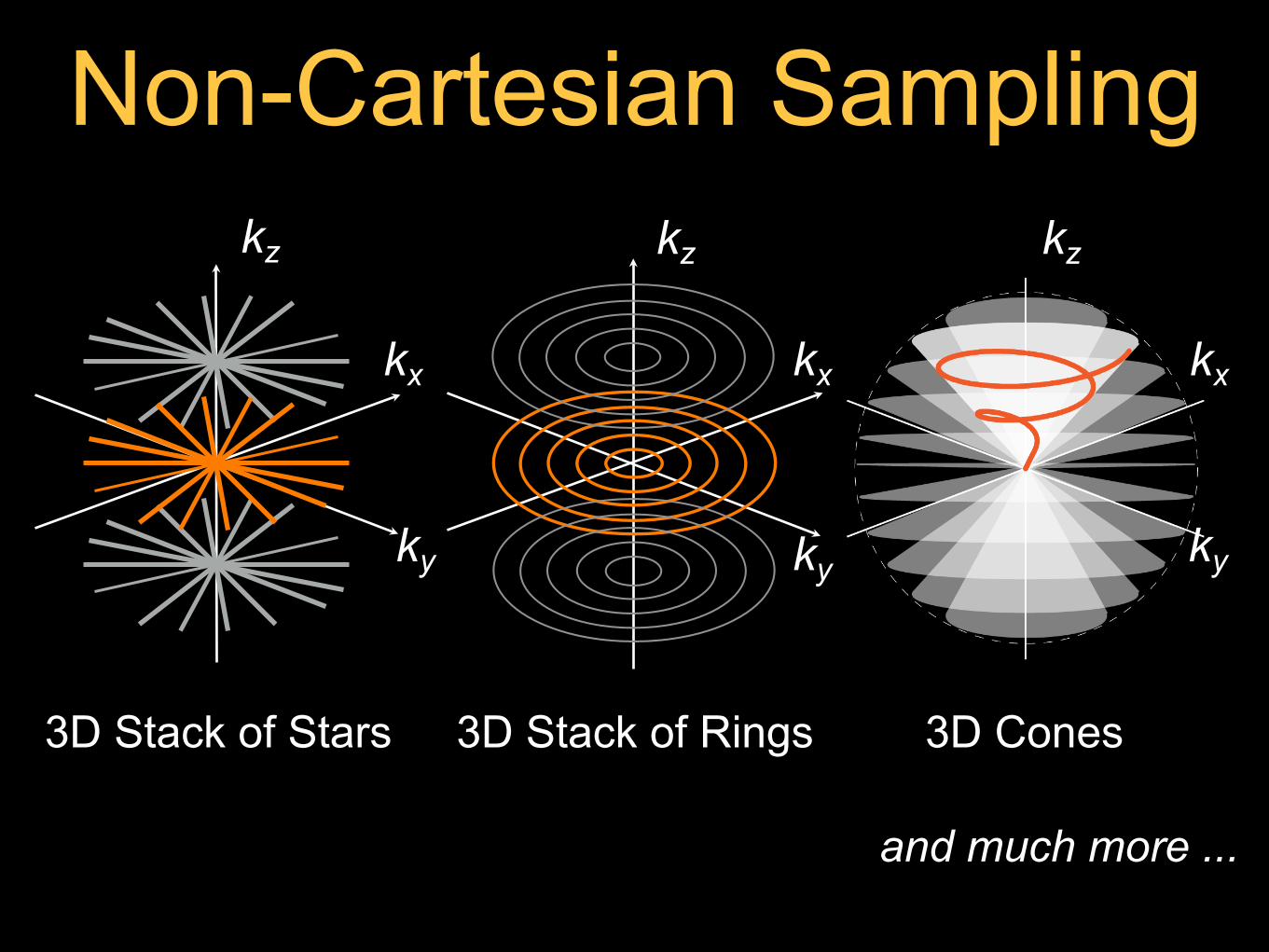
Non-Cartesian Sampling

3D Cones

kz

kx

ky

kz

kx

ky

3D Stack of Rings

and much more ...

kz

kx

ky

3D Stack of Stars

3D Stack-of-Radialkz

kx

ky

Pros - Straightforward extension of radial - Robust to motion - Can tolerate a lot of undersampling Cons - May have mixed contrast - Sensitive to gradient delays - Sensitive to off-resonance effects

aka Stack-of-Stars

3D Stack-of-Radial: Liver MRI

courtesy of Tess Armstrong

Axial

Coronal

Sagittal

Free-breathing 3D Liver MRI; FLASH at 3 T

3D Radialkz

kx

ky

image from http://en.wikipedia.org/wiki/Koosh_ball

Pros - Robust to motion (get DC every TR) - Can tolerate a lot of undersampling - Half-spoke PR has very short TE Cons - May have mixed contrast - Sensitive to gradient delays - Sensitive to off-resonance effects

3D Radial: Coronary MRAContrast-Enhanced at 3.0T

ECG-gated, fat-saturated, inversion-recovery prepared spoiled gradient echo sequence(1.0 mm)3 spatial resolution, 1D self navigation, CG-SENSE recon, 5.4 min scan time

courtesy of Debiao Li and J Pang (Cedars-Sinai)

3D Coneskz

kx

ky

Pros - Very fast (3-8x vs. Cartesian) - Very short TE - Flexible readout length - Robust to motion/flow effects Cons - May have mixed contrast - Sensitive to gradient delays - Sensitive to off-resonance effects

Gurney PT et al., MRM 2006; 55: 575-82

3D Cones: Coronary MRA3D Cones Sequence - 1.5 T; 8-ch cardiac array - ATR-SSFP - FOV 28x28x14 cm3 - RES 1.2x1.2x1.25 mm3 - 9142 TRs (~3x speedup) - 100 ms phase(s) - 3D motion compensation - <10 min scan

Wu HH et al., MRM 2013; 69: 1083-1093

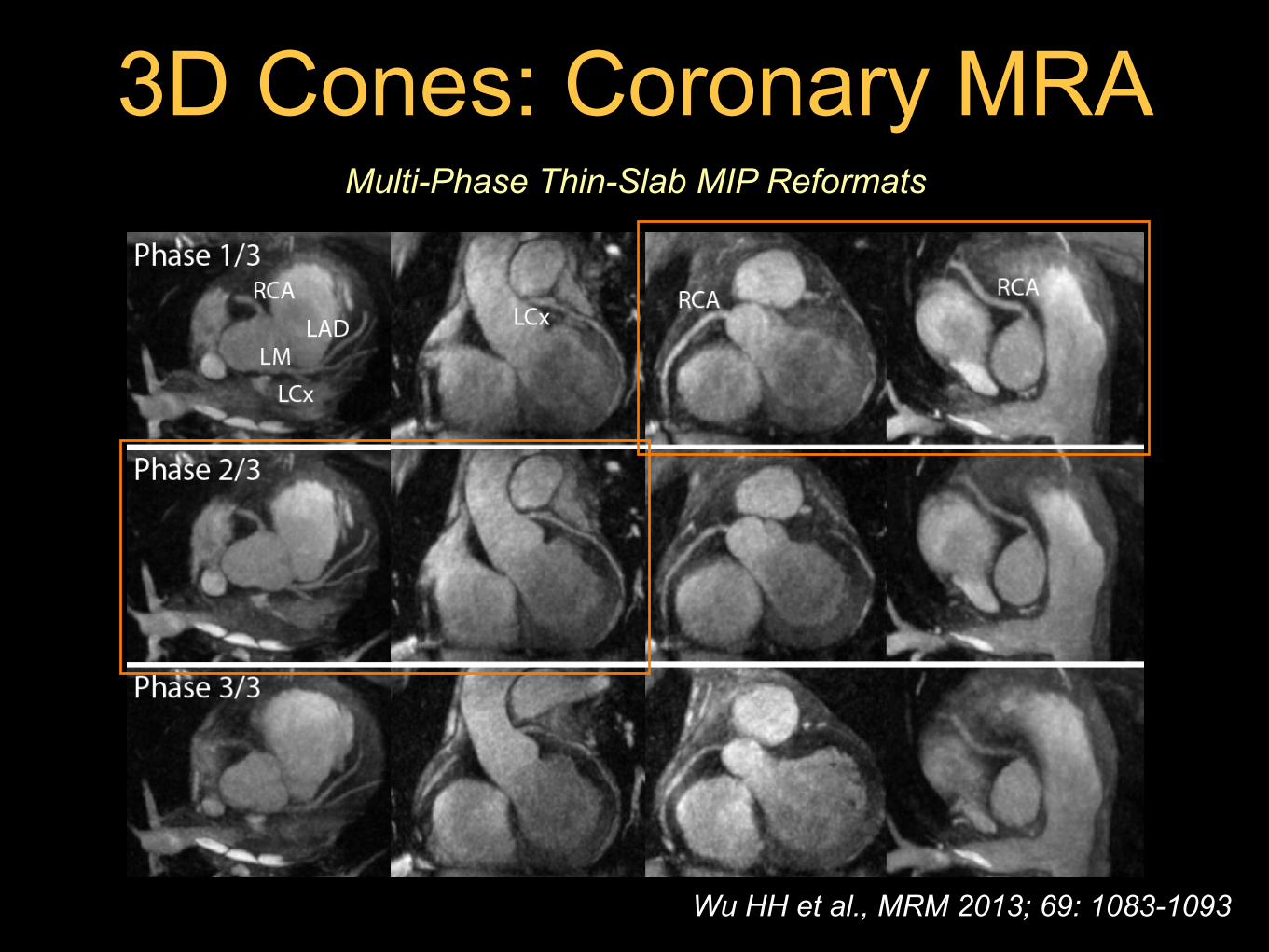
3D Cones: Coronary MRAMulti-Phase Thin-Slab MIP Reformats

Wu HH et al., MRM 2013; 69: 1083-1093

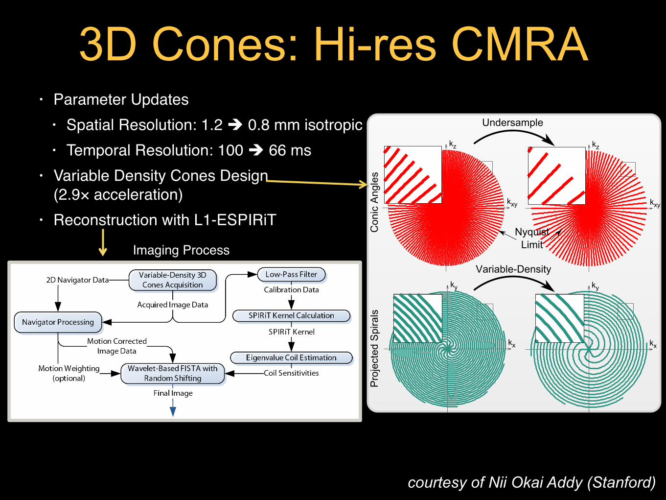
3D Cones: Hi-res CMRA• Parameter Updates

• Spatial Resolution: 1.2 ! 0.8 mm isotropic • Temporal Resolution: 100 ! 66 ms

• Variable Density Cones Design (2.9× acceleration)

• Reconstruction with L1-ESPIRiTkxy

kz

kxy

kz

Undersample

Variable-Density

kx

ky

kx

ky

NyquistLimit

Con

ic A

ngle

sPr

ojec

ted

Spira

ls

Imaging Process

courtesy of Nii Okai Addy (Stanford)

3D Cones: Hi-res CMRAThin-Slab MIP Reformats: 0.8 mm isotropic

Subject A Subject B Subject C

1.2 mm 0.8 mmRight coronary

artery cross section

1.5 T; 8-channel cardiac coil

courtesy of Nii Okai Addy (Stanford)

Non-Cartesian Image Reconstruction

• Gridding reconstruction

• Gradient measurement

• Off-resonance correction (if time permits)

MRI Signal Equation

kx(t) =�

2⇡

Z t

0Gx(⌧) d⌧, ky(t) =

�

2⇡

Z t

0Gy(⌧) d⌧

General definition of k-space:

s(t) =

ZZ

X,Y

m(x, y) · exp(�i2⇡ · [kx(t)x+ ky(t) y]) dx dy

= FT (m(x, y) ) = M( kx(t), ky(t) )

m(x, y) =

ZZ

kx,ky

M(kx, ky) · exp(i2⇡ · [kxx+ kyy]) dkx dky

m(x, y) = FT �1(M(kx, ky) )

MRI Reconstruction

simple for Cartesian (kx, ky) to Cartesian (x, y): 2D FFT

time consuming for non-Cartesian (kx, ky) to Cartesian (x, y)

k-space image space

uniform

non-uniform

uniform

non-uniform

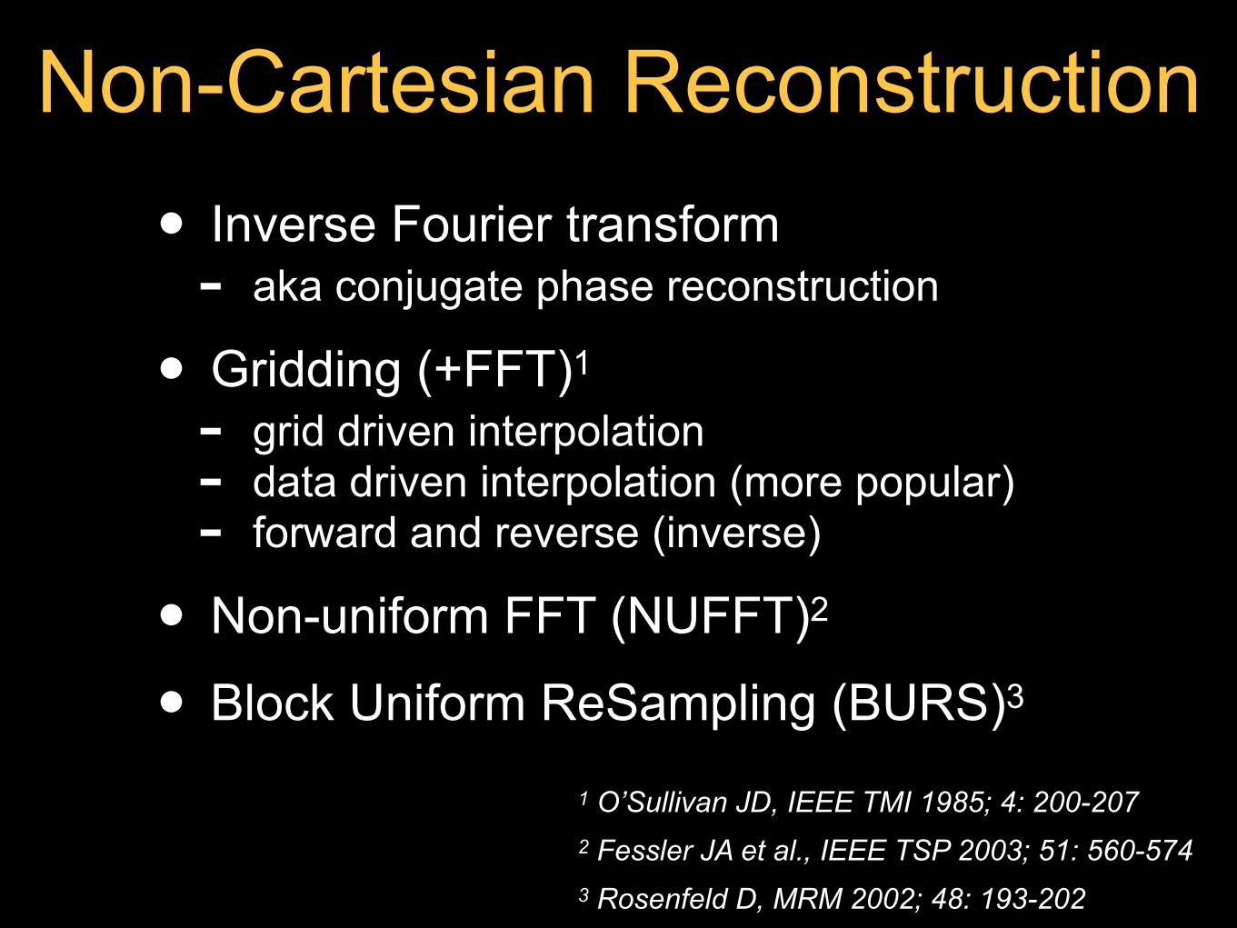
Non-Cartesian Reconstruction• Inverse Fourier transform

- aka conjugate phase reconstruction

• Gridding (+FFT)1 - grid driven interpolation - data driven interpolation (more popular) - forward and reverse (inverse)

• Non-uniform FFT (NUFFT)2

• Block Uniform ReSampling (BURS)3

2 Fessler JA et al., IEEE TSP 2003; 51: 560-5743 Rosenfeld D, MRM 2002; 48: 193-202

1 O’Sullivan JD, IEEE TMI 1985; 4: 200-207

Gridding: Basic Idea

convolve each acquired data point with kernel C(kx, ky)

k-spaceC(kx, ky)

resample the convolution onto Cartesian grid points2D inverse FFT; de-apodization and FOV cropping

Gridding: Basic MathTo the board …

Gridding: Basic MathS(kx, ky) =

X

j

2�(kx � kx,j , ky � ky,j)

M(kx, ky) = [(M(kx, ky) · S(kx, ky)) ⇤ C(kx, ky)] · III(kx�kx

,ky�ky

)

non-Cartesian dataset interpolation resample to grid

Sampling pattern:

C(kx, ky)Convolution kernel:

Gridding recon:

m(x, y) = [(m(x, y) ⇤ s(x, y)) · c(x, y)] ⇤ III( x

FOVx,

y

FOVy)

remove by croppingremove by deap! m(x, y)

III(kx�kx

,ky�ky

)Grid:

FFT

Gridding: Design Issues

• Convolution kernel - apodization; aliasing

• Sampling grid density (Cartesian) - aliasing

• Sampling pattern (non-Cartesian) - impulse response and side lobes - density characterization / compensation

Gridding: Design - Kernel

• Ideal convolution kernel: SINC - don’t need de-apodization - infinite extent impractical to implement - windowed version has limited performance

• Desired kernel characteristics - compact support (finite width) in k-space - minimal aliasing effects in image (sharp

transition)

Gridding: Design - Kernel

�kx =1

FOVx,�ky =

1

FOVy

Combine with grid oversampling

�kx↵

=1

↵FOVx,�ky↵

=1

↵FOVy↵ > 1

M(kx, ky) = [(M(kx, ky) · S(kx, ky)) ⇤ C(kx, ky)] · III(kx

�kx/↵,

ky�ky/↵

)

m(x, y) = [(m(x, y) ⇤ s(x, y)) · c(x, y)] ⇤ III( x

↵FOVx,

y

↵FOVy)

Gridding: Design - KernelCombine with grid oversampling

object ……

α = 2 very forgiving; many kernels work well; apodization minimalexpensive … especially for 3D gridding

c(x,y)

object replica

αFOV

c(x,y)……

replica

FOValiasing

replicas from resampling to gridFOVcause additional aliasing

Gridding: Design - Kernel

• Jointly consider α and kernel - minimize aliasing energy - characterize trade-offs - numerical designs possible - Kaiser-Bessel window works very well, with

proper choice of β and kw1,2; precompute a lookup table to speedup calculations2

2Beatty et al., IEEE TMI 2005; 24: 799-808

1Jackson et al., IEEE TMI 1991; 10: 473-478

CKB(kx) = I0

�

s

1� (kx

kw/2)2

!

Gridding: Design - DensitySampling density of S(kx, ky) not uniform: ⇢(kx, ky)

M(kx, ky) = [(M(kx, ky) ·S(kx, ky)

⇢(kx, ky)) ⇤ C(kx, ky)] · III

Pre-compensation of sampling density:

density corrected on a data point basis before convolutionneed to know ⇢(kx, ky)

from geometrical analysis, numerical analysis (Voronoi), etc.

inverse of ρ known as the density compensation function (DCF)

M(kx, ky) =[(M(kx, ky) · S(kx, ky)) ⇤ C(kx, ky)] · III

⇢(kx, ky)

Gridding: Design - DensityPost-compensation of sampling density:

density corrected on a grid point basis after convolutioncan estimate ρ along with gridding; grid all 1s:

… but only an approximation and fails when S changes rapidly

⇢(kx, ky) = [S(kx, ky) ⇤ C(kx, ky)] · III

may be okay if S changes slowly

Gridding: 2D Radial ExampleRadial trajectory [256x256] with ramp DCF

Gridding: 2D Radial Example

α = 2; grid size = 2x[256 256]; kw = 4;

Kaiser-Bessel convolution kernel with linear lookup table1

1Beatty et al., IEEE TMI 2005; 24: 799-808

showing 1D & one side

Gridding: 2D Radial ExampleGridded data on [512x512] grid

Gridding: 2D Radial ExampleInverse 2D FFT produces image with 2x FOV

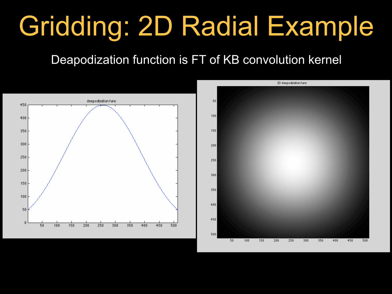
Gridding: 2D Radial ExampleDeapodization function is FT of KB convolution kernel

Gridding: 2D Radial ExampleDeapodized image

Gridding: 2D Radial ExampleFOV cropped to extract desired [256x256] image

α = 2, kw = 4

Gridding: 2D Radial ExampleFOV cropped to extract desired [256x256] image

α = 1.375, kw = 51

1Beatty et al., IEEE TMI 2005; 24: 799-808

Gridding: Summary

• Data input - k-space data - k-space traj (usually normalized), DCF

• Gridding params - target image dimensions [MxN] - grid oversampling factor α - kernel type and width

• Data output - gridded Cartesian k-space - reconstructed image

Gradient Measurement

• Non-Cartesian recon requires - k-space trajectory - density compensation function

• Both depend on actual gradient waveforms on scanner - can deviate from desired

• Knowledge of k-space trajectory also important for RF design

Gradient Measurement

• Gradient imperfections cause artifacts - FOV scaling, shifting - signal loss, shading - image blurring, geometric distortion

• Sources of gradient errors - eddy currents (B0, linear) - group delays (RF filters, A/D) - amplifier limitations (BW, freq response) - gradient warping - other ...

Gradient Measurement

• General techniques - off-iso slice technique1,2, and more

• Trajectory-specific techniques - radial3, spiral4, and more

• Characterize gradient system - assume linear time-invariant model5

5 Addy NO et al., MRM 2012; 68: 120-129

4 Robison RK et al., MRM 2010; 63: 1683-90

3 Peters DC et al., MRM 2003; 50: 1-6

2 Beaumont M et al., MRM 2007; 58: 200-205

1 Duyn JH et al., JMR 1998; 132: 150-153

Gradient Measurement

• Trajectory-specific delay calibration

Gradient MeasurementOff-isocenter slice measurement technique

Duyn JH et al., JMR 1998; 132: 150-153

test waveform

signal

G

RF

ADC

x1

Can repeat on all three axes Gx, Gy, Gz

Δx

Gradient MeasurementOff-isocenter slice measurement technique

Duyn JH et al., JMR 1998; 132: 150-153

Waveform ON:

Phase difference:

��x1(t) = �

Z t

0G(⌧) · x1 d⌧ = x1 · k(t)

sx1,Gon(t) =

ZZ

Y,Z

m(x1, y, z)e�i�0(x1,y,z,t) · e�i2⇡·[ �

2⇡

R t0 G(⌧)d⌧ ]·x1 dy dz

Waveform OFF:

sx1,Goff (t) =

ZZ

Y,Z

m(x1, y, z)e�i�0(x1,y,z,t) dy dz

Gradient Measurement

Gradient Measurement• Gradient (trajectory) correction - use actual trajectory for recon - pre-tune bulk gradient delay

Calculated TrajectoryNominal Trajectory Difference (x8)

Example: Axial Spiral at 1.5 T

Addy NO et al., MRM 2012; 68: 120-129

Gradient Measurement

• Off-iso slice measurement technique - two measurements per axis - can measure X on X, Y on Y, Z on Z, and

also cross terms; linearly combine - Δx should be small (may need avging) - need to account for phase wrapping - use spin echo for long waveforms - can acquire multiple slice offsets and

gradient polarities to model individual gradient error terms

Gradient Measurement

• Delay calibration - gradient errors (e.g., linear eddy currents)

mainly cause an apparent bulk delay - adjust ADC window w.r.t. gradients - delays may be different for each axis

s(t) =

ZZ

X,Y

m(x, y) · e�i�(x,y,t) · e�i2⇡·[kx(t) x+ky(t) y] dx dy

Off-resonance Correction • Off resonance effects (ΔB0, fat, etc.)

- patient (scan) dependent - pre-scan shim calibration helps - usually negligible for Cartesian MRI - non-Cartesian MRI: signal loss,

spatial blurring, geometric distortion

�(x, y, t) = 2⇡ (x, y)t

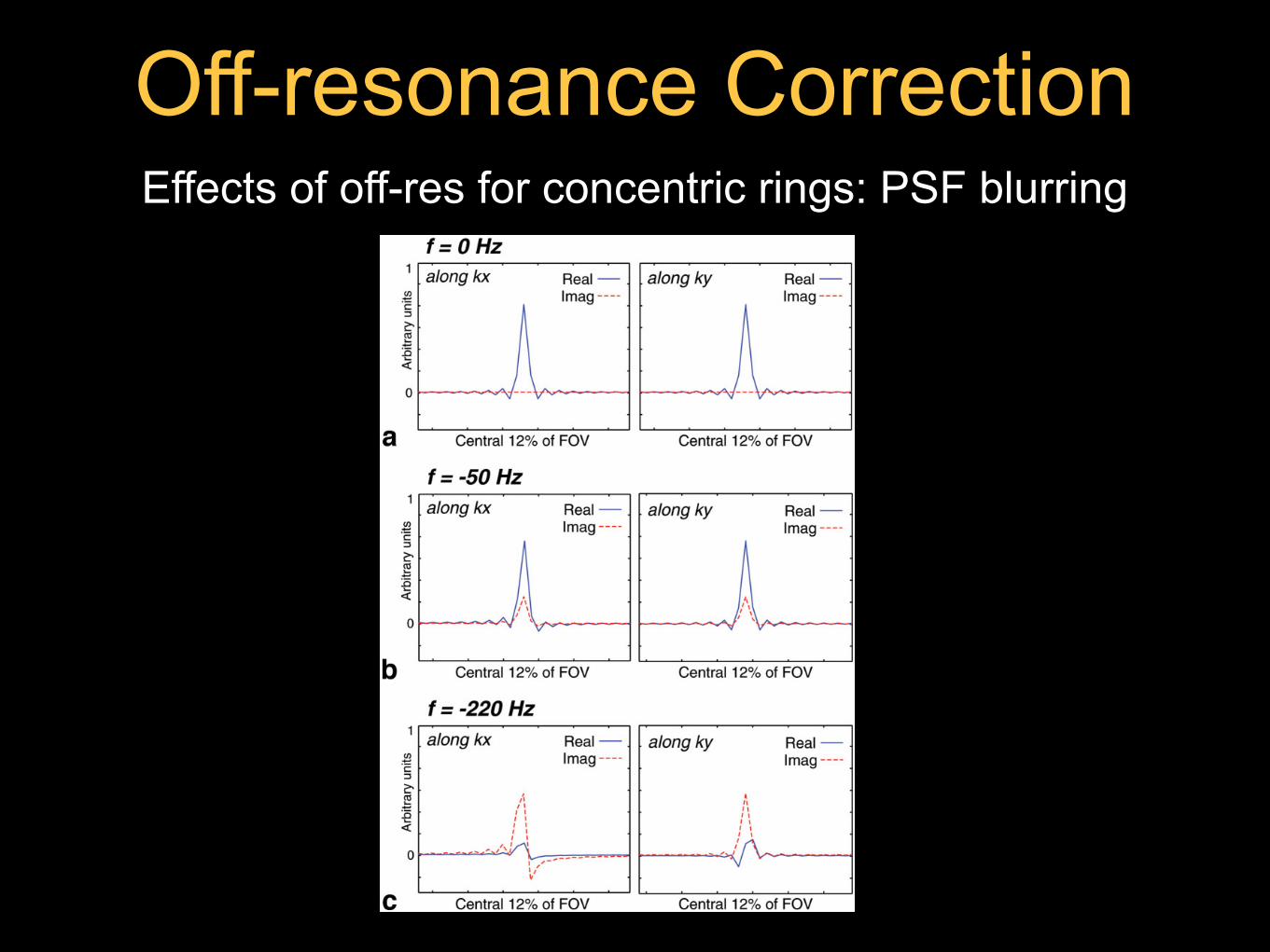
Off-resonance Correction Effects of off-res for concentric rings: PSF blurring

• Account for field inhomogeneity - use shorter readouts - measure/estimate field mapand then correct (during recon)1,2,3

time-segmented, freq-segmented, etc.

Off-resonance Correction

1 Noll DC et al., IEEE TMI 1991; 10: 629-637

3 Chen JY et al., MRM 2011; 66: 390-401

s(TE1) �! I1 = M 0(x, y) · e�i2⇡ (x,y)TE1

s(TE2) �! I2 = M 0(x, y) · e�i2⇡ (x,y)TE2

(x, y) = arg(I1 · I⇤2 )/2⇡(�TE) [±1/2⇡�TE ]

2 Noll DC et al., MRM 1992; 25: 319-333

Off-resonance Correction Linear Correction

(x, y) = f0 + fxx+ fyy (can fit to this model)

�(x, y) = 2⇡f0t+ 2⇡�kx(t)x+ 2⇡�ky(t)y

�kx(t) = fxt, �ky(t) = fyt

s(t) = e�i2⇡f0t

ZZ

X,Y

m(x, y) · e�i2⇡·[(kx(t)+�kx(t)) x+(ky(t)+�ky(t)) y] dx dy

demod shift k-space trajectory

Irarrazabal P et al., MRM 1996; 35: 278-282

Can follow with frequency-segmented off-res correction

Off-resonance Correction Frequency-segmented correction

Bernstein et al., Handbook of MRI Sequences, Fig. 17.63

Off-resonance Correction Time-segmented correction

Bernstein et al., Handbook of MRI Sequences, Fig. 17.64

Off-resonance Correction

Regular Recon Field Map ORC Image

Example: Axial Concentric Rings at 1.5 T

Wu HH et al., MRM 2008; 59: 102-112

Off-resonance Correction• Field map measurement

• Segmented correction methods - Need to recon multiple images,

Nbins ~ 4(fmax - fmin)Tacq

• Other sources of off resonance - concomitant gradients - chemical shift (next lecture)

• Other ORC algorithms - autofocusing (field map optional) - combine with image reconstruction

Thanks!

• Further reading - references on each slide - further reading section on website

• Acknowledgments - John Pauly’s EE369C class notes (Stanford)

Holden H. Wu, Ph.D.

HoldenWu@mednet.ucla.edu

http://mrrl.ucla.edu/wulab