Fast Fourier Transform in Predicting Financial Securities Prices

University of Utah

May 3, 2016

Michael Barrett Williams

Introduction

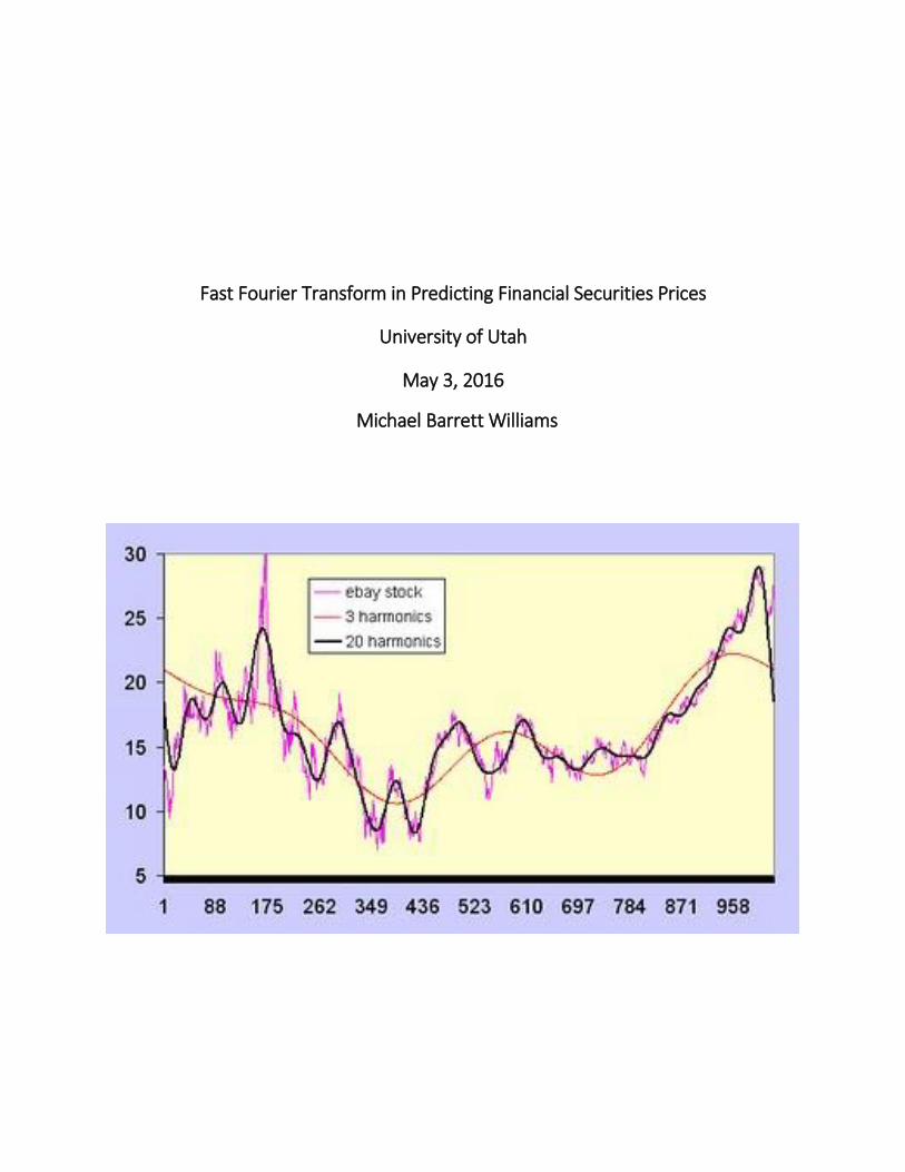
The Fast Fourier Transform (FFT) is a fascinating algorithm that is used for predicting the

future values of data. The algorithm computes the Discrete Fourier Transform of a sequence or

its inverse, often times both are performed. Fourier analysis transforms a signal from the

domain of the given data, usually being time or space, and transforms it into a representation

of frequency.

The FFT Algorithm: ∑ 𝑎2𝑛𝑒−2𝜋(2𝑛)𝑖𝑘

𝑁 +𝑁

2−1

𝑛=0∑ 𝑎2𝑛+1𝑒

−2𝜋(2𝑛+1)𝑖𝑘

𝑁

𝑁

2−1

𝑛=0

In the financial field the FFT is used in computational finance mostly, for predicting the

prices of financial derivatives on a time series basis. A financial derivative is an openly traded

security that is backed by multiple assets or other securities. The most common one is an

“option.” When performing Fourier analysis on a financial derivatives one would take the

Discrete Fourier Transform of the specific security and then take the Inverse Fourier Transform

to get the future prices of the security. An individual would then make trades based of this

data. These strategies are used by quant groups inside of Investment Banks, such as Morgan

Stanley and Goldman Sachs, as well as quantitative hedge funds. More robust strategies for

predicting and valuing these financial derivatives exist, but this is a base strategy.

The following steps will be a brief explanation of how the FFT is used to price a near-the-money

option call (Carr and Madan, 67).

The FFT algorithm for pricing an option: 𝜔𝑘 = ∑ 𝑒−1(2𝜋

𝑁)(𝑗−1)(𝑘−1)

𝑋(𝑗) 𝑁𝑗=1 for k=1,…,N

N is typically a power of 2. The algorithm reduces it from 𝑁^2 to 𝑁𝑙𝑛_2 (𝑁).

The approximation of the call price is: 𝐶𝑇(𝑘) ≈exp(−𝛼𝑘)

𝜋∑ 𝑒−𝑖𝑣𝑗𝑘𝛹𝑇(𝑣𝑗)𝜂𝑁

𝑗=1

The upper limit for integration is now 𝑎=𝑁𝜂. We are mostly focusing on near-the-money calls

with this integration. The FFT returns N values of k and we will then employ normal spacing of

size λ, this gives us k values of:

𝑘𝑢 = −𝑏 + 𝜆(𝑢 − 1) for u=1,…,N

This returns log strike levels from –b to b, where 𝑏 =1

2𝑁𝜆.

Incorporate Simpson's rule of weighting into the summation and the restriction 𝜆𝜂 =2𝜋

𝑁, the

call price can be rewritten as:

𝐶𝑇(𝑘𝑢) ≈exp(−𝛼𝑘𝑢)

𝜋∑ 𝑒−𝑖𝑣𝑗𝑘𝛹𝑇(𝑣𝑗) (

𝜂

3) [3 + (−1)𝑗 − 𝛿𝑗−1]

𝑁

𝑗=1

Where 𝛿𝑛 is the Kronecker delta function that is unity for n=0 and zero otherwise.

“The use of the FFT for calculating out-of-the-money option prices is similar to 𝐶𝑇(𝑘𝑢). The only

differences are that we replace the multiplication by exp(−𝛼𝑘𝑢) with a division by sinh (𝛼𝑘)

and the function call to 𝛹(𝑣) is replaced by a function call to 𝛾𝑡(𝑣) =ζ𝑇(𝑣−𝑖𝛼)−ζ𝑇(𝑣+𝑖𝛼)

2” (Carr

and Madan, 68).

In my analysis, I performed the FFT on a plain vanilla equity, which is very uncommon in

quantitative finance. This is because there is not a lot of mathematical data one can draw upon

to help predict future values, that is why they are mostly performed on derivatives. Also,

professional companies will likely have more data in their models than just stock price, which is

what I chose to do.

Model and Method

I implemented the FFT model to predict the future values of a stock price. I did a couple

of different lengths of time for my data sets. I will mainly be talking about the data set where I

used the closing stock price of 415 sequential trading days to predict prices for the following 90

trading days. The model uses a least squares regression to find the line of best fit for the data.

The maximum power of the line of best fit was three. I analyzed the curves from linear,

quadratic, and cubic functions and determined which one I wanted to use based off how well it

fit the data. When implementing this process, I only ever used a quadratic or cubic function to

model my data. I found the linear model was never sufficient in predicting the prices because of

the volatility that was encountered in the stock market. Also, when using the cubic functions,

sometimes they too were not sufficient because the function tried to follow to peaks and

troughs too closely. This would cause the best fit line to go to infinity or zero before trying to

map the rest of the data points causing the predicted values received from taking the inverse

transform to be extremely inaccurate.

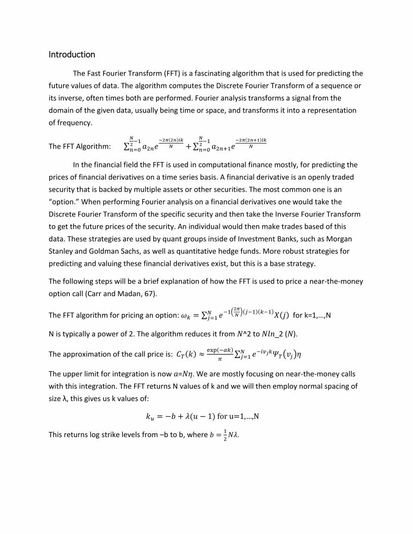
This is the stock price for Palo Alto Networks (PANW). A cubic function was the best fit for the

data. In this case, it maps the data pretty well, even though the market is going through a

volatile state.

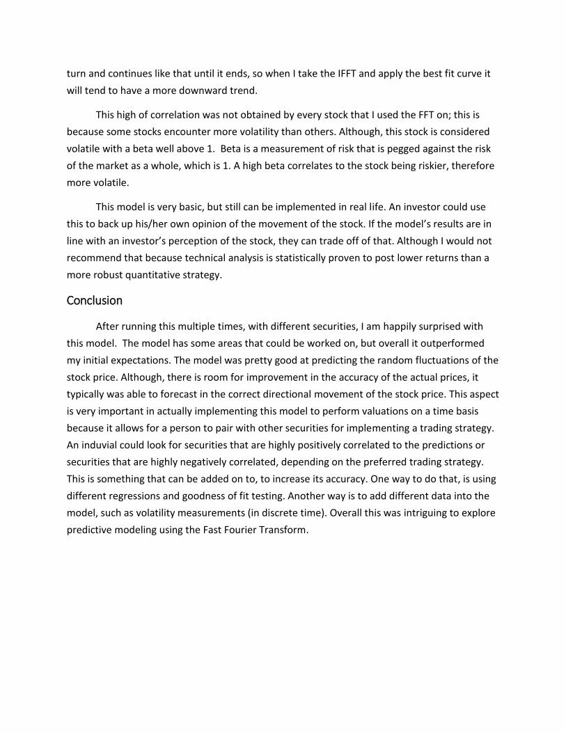
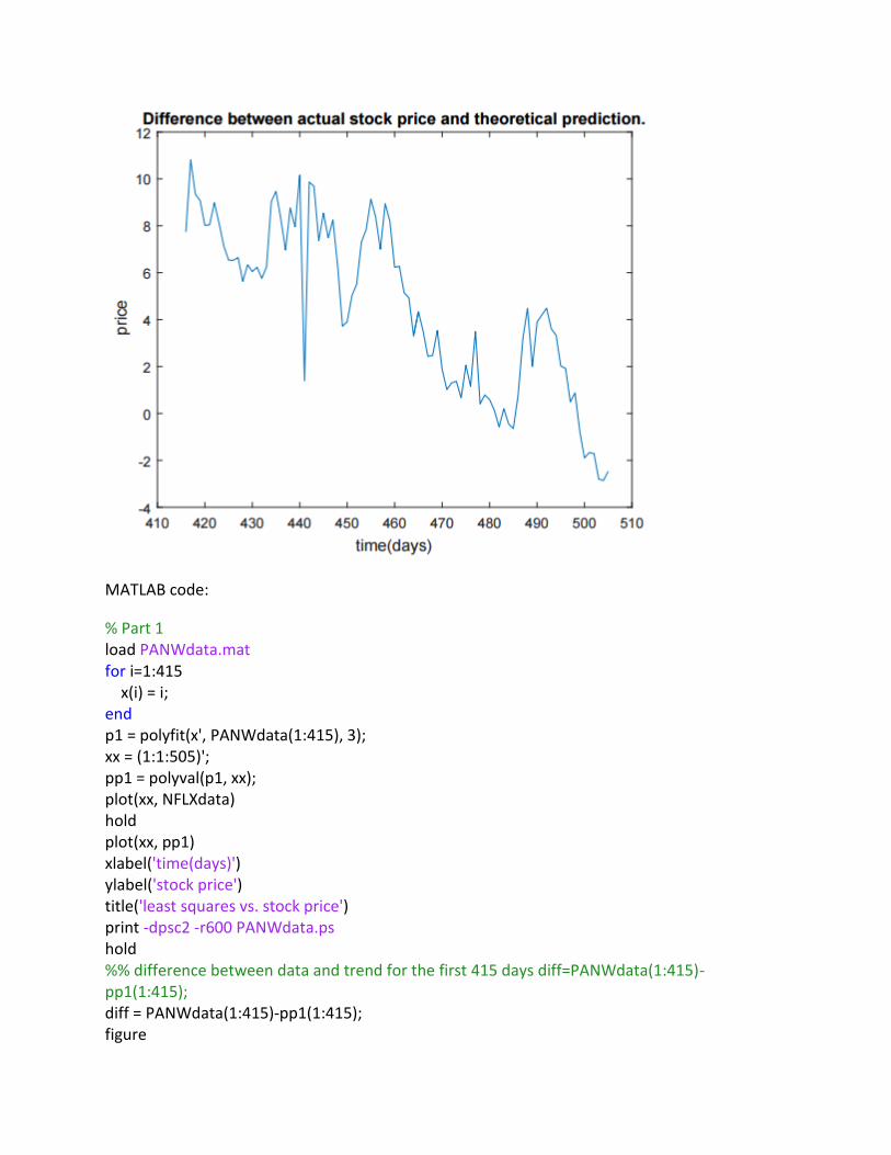
The second chart on this page shows the difference between the regression and the actual

stock price. This is how I determined which type of function to use. I picked the one that was

more accurate.

This is a graph of the absolute values of the FFT of the graph above. This is the initial step of the

algorithm, where it take the Discrete Fourier Transform. This is the representation of the time

series data in frequency of the sinusoidal curve depicting the transformed data.

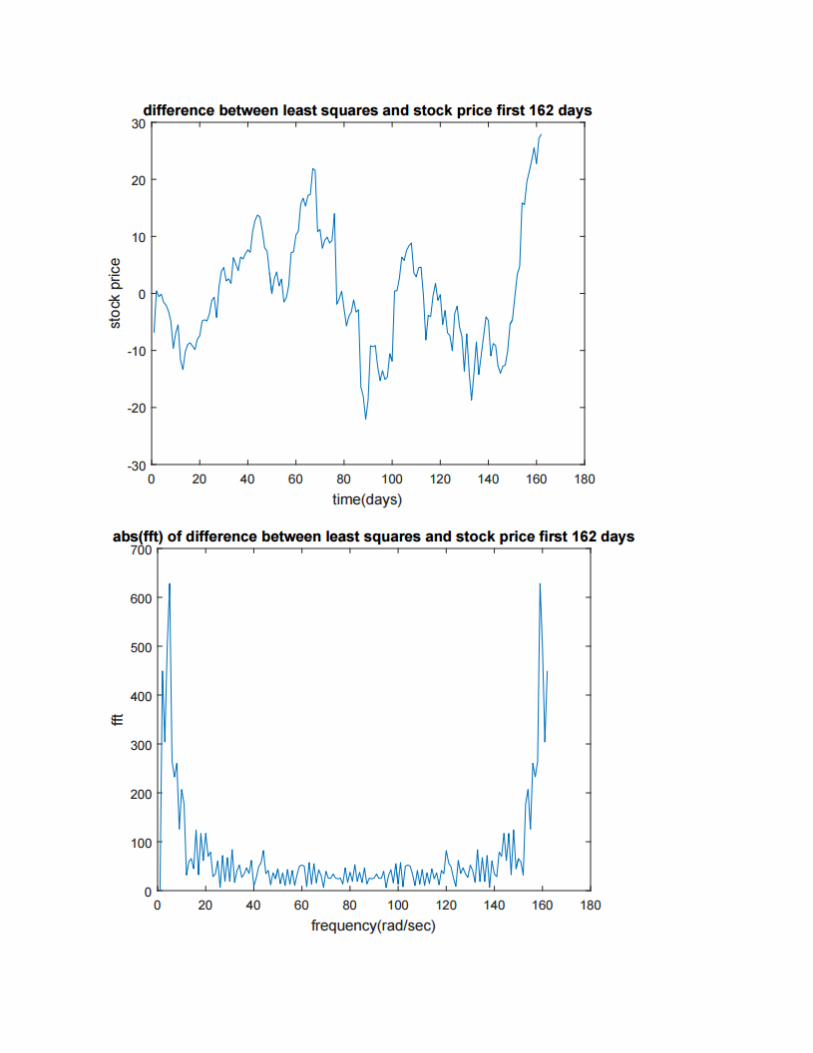
Then I took the Inverse FFT of the cleaned data. In this case, I chose to leave all the data points

in the model. This is why the difference is essentially zero, I took the IFFT of the FFT data and

since I did not clean the data it theoretically should be the same. The reason it is not zero is

presumed to be a rounding error in MATLAB.

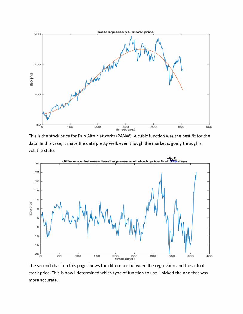
Next I interpolate the data for the 90 days that the model is trying to predict, this is

done by taking the Discrete Fourier Transformation with the equation form of:

a(k)=real(Y(k));

b(k)=-imag(Y(k));

omk=2*pi*(k-1)/365;

YY(n)=YY(n)+a(k)*cos(omk*(n-1))+b(k)*sin(omk*(n-1));

Using this a person is able to interpolate the IFFT curve obtained from the first 415 days and

use it to interpolate the following 90 days. The interpolation is then added to the best fit curve

obtained from the least squares regression for the next 90 days out. When this is done by the

program, it shows us how the stock price will fluctuate for the ensuing 90 day time period.

I obtained the theoretical (predicted) values (red) by taking the IFFT of the curve I got

from the first 415 days. I then used this to interpolate the next 90 days of data and plotted it

against the actual 90 days (blue). I obtained a 62% correlation, but my percent error was much

lower than expected for only having a 62.7% correlation. I had a 12.4% error of average of the

90 interpolated data points. This model is fairly good a predicting the swing of the stock price.

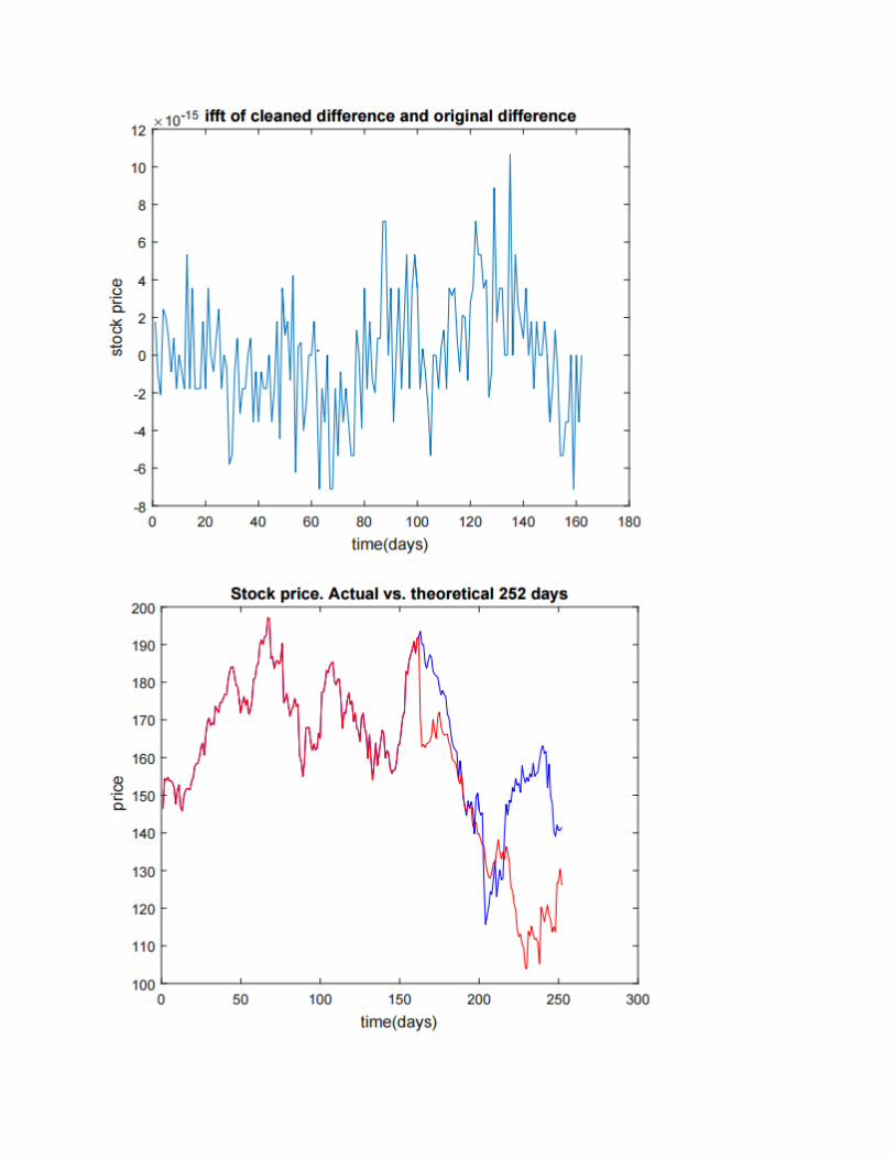
When looking at this graph, one can see that it models the decline in price very well, but it does

not catch the rebound of the price like we see in actual data for those 90 days. I believe this can

be attributed to the long linear increase of the price. Also, the best fit line takes a downward

turn and continues like that until it ends, so when I take the IFFT and apply the best fit curve it

will tend to have a more downward trend.

This high of correlation was not obtained by every stock that I used the FFT on; this is

because some stocks encounter more volatility than others. Although, this stock is considered

volatile with a beta well above 1. Beta is a measurement of risk that is pegged against the risk

of the market as a whole, which is 1. A high beta correlates to the stock being riskier, therefore

more volatile.

This model is very basic, but still can be implemented in real life. An investor could use

this to back up his/her own opinion of the movement of the stock. If the model’s results are in

line with an investor’s perception of the stock, they can trade off of that. Although I would not

recommend that because technical analysis is statistically proven to post lower returns than a

more robust quantitative strategy.

Conclusion

After running this multiple times, with different securities, I am happily surprised with

this model. The model has some areas that could be worked on, but overall it outperformed

my initial expectations. The model was pretty good at predicting the random fluctuations of the

stock price. Although, there is room for improvement in the accuracy of the actual prices, it

typically was able to forecast in the correct directional movement of the stock price. This aspect

is very important in actually implementing this model to perform valuations on a time basis

because it allows for a person to pair with other securities for implementing a trading strategy.

An induvial could look for securities that are highly positively correlated to the predictions or

securities that are highly negatively correlated, depending on the preferred trading strategy.

This is something that can be added on to, to increase its accuracy. One way to do that, is using

different regressions and goodness of fit testing. Another way is to add different data into the

model, such as volatility measurements (in discrete time). Overall this was intriguing to explore

predictive modeling using the Fast Fourier Transform.

Work Cited

Carr, P., & Madan, D. B. (1999). Option valuation using the fast Fourier transform (pp. 61-73,

Rep. No. Volume 2, Issue 4). New York City, NY: New York University. Retrieved April 18,

2015, from http://www.math.nyu.edu/research/carrp/papers/pdf/jcfpub.pdf

Wojtak, A. (2007). Attempt To Predict the Stock Market: An Interactive Qualifying Project

Report(Master's thesis, Worcester Polytechnic Institute, 2007) (pp. 1-65). Worcester

Polytechnic Institute. doi: https://www.wpi.edu/Pubs/E-project/Available/E-project-

022808-142909/unrestricted/FullIQPReport7.pdf

Appendix

Palo Alto Networks (215 Trading days):

Correlation: 55.4%

Percent Error (for Predictions): 15.5%

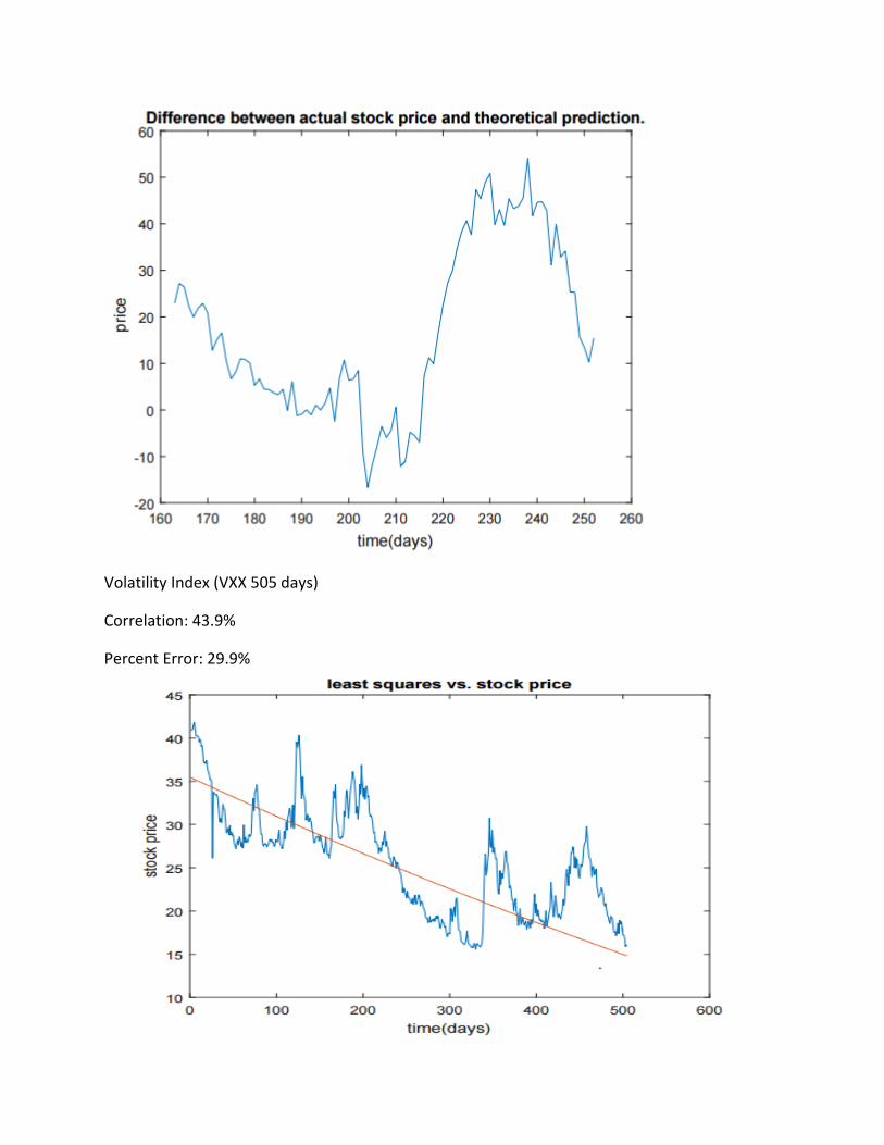
Volatility Index (VXX 505 days)

Correlation: 43.9%

Percent Error: 29.9%

MATLAB code:

% Part 1 load PANWdata.mat for i=1:415 x(i) = i; end p1 = polyfit(x', PANWdata(1:415), 3); xx = (1:1:505)'; pp1 = polyval(p1, xx); plot(xx, NFLXdata) hold plot(xx, pp1) xlabel('time(days)') ylabel('stock price') title('least squares vs. stock price') print -dpsc2 -r600 PANWdata.ps hold %% difference between data and trend for the first 415 days diff=PANWdata(1:415)-pp1(1:415); diff = PANWdata(1:415)-pp1(1:415); figure

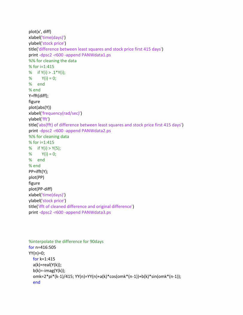
plot(x', diff) xlabel('time(days)') ylabel('stock price') title('difference between least squares and stock price first 415 days') print -dpsc2 -r600 -append PANWdata1.ps %% for cleaning the data % for i=1:415 % if Y(i) > .1*Y(i); % Y(i) = 0; % end % end Y=fft(diff); figure plot(abs(Y)) xlabel('frequency(rad/sec)') ylabel('fft') title('abs(fft) of difference between least squares and stock price first 415 days') print -dpsc2 -r600 -append PANWdata2.ps %% for cleaning data % for i=1:415 % if Y(i) > Y(5); % Y(i) = 0; % end % end PP=ifft(Y); plot(PP) figure plot(PP-diff) xlabel('time(days)') ylabel('stock price') title('ifft of cleaned difference and original difference') print -dpsc2 -r600 -append PANWdata3.ps %interpolate the difference for 90days for n=416:505 YY(n)=0; for k=1:415 a(k)=real(Y(k)); b(k)=-imag(Y(k)); omk=2*pi*(k-1)/415; YY(n)=YY(n)+a(k)*cos(omk*(n-1))+b(k)*sin(omk*(n-1)); end

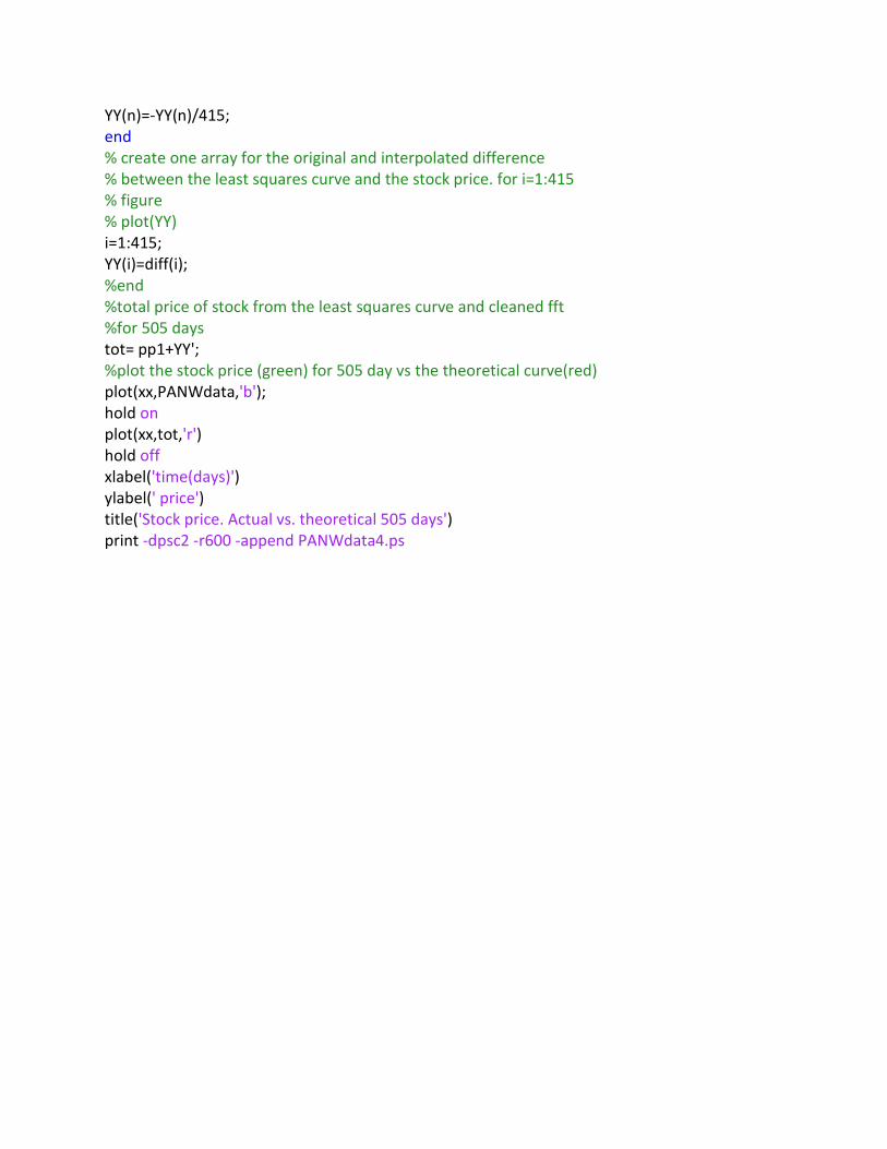
YY(n)=-YY(n)/415; end % create one array for the original and interpolated difference % between the least squares curve and the stock price. for i=1:415 % figure % plot(YY) i=1:415; YY(i)=diff(i); %end %total price of stock from the least squares curve and cleaned fft %for 505 days tot= pp1+YY'; %plot the stock price (green) for 505 day vs the theoretical curve(red) plot(xx,PANWdata,'b'); hold on plot(xx,tot,'r') hold off xlabel('time(days)') ylabel(' price') title('Stock price. Actual vs. theoretical 505 days') print -dpsc2 -r600 -append PANWdata4.ps