Fast Dynamic Programming for Labeling Problems with Ordering Constraints

Junjie Bai∗ Qi Song∗ Olga Veksler† Xiaodong Wu∗

∗Department of Electrical and Computer EngineeringThe University of Iowa

junjie-bai, qi-song, xiaodong-wu@uiowa.edu

†Computer Science DepartmentUniversity of Western Ontario

olga@csd.uwo.ca

Abstract

Many computer vision applications can be formulatedas labeling problems. However, multilabeling problems areusually very challenging to solve, especially when some or-dering constraints are enforced. We solve in this papera five-parts labeling problem proposed in [6, 7]. In thismodel, one wants to find an optimal labeling for an imagewith five possible parts: “left”, “right”, “top”, “bottom”and “center”. The geometric ordering constraints can beread naturally from the names. No previous method cansolve the problem with globally optimal solutions in a lin-ear space complexity. We propose an efficient dynamic pro-gramming based algorithm which guarantees the global op-timal labeling for the five-parts model. The time complexityis O(N1.5) and the space complexity is O(N), with N be-ing the number of pixels in the image. In practice, it runsfaster than previous methods. Moreover, it works for both4-neighborhood and 8-neighborhood settings, and can beeasily parallelized for GPU.

1. Introduction

Given an image, the multilabeling problem seeks to as-sign a label to each pixel from a set of fixed labels, which,in general, is NP-hard [1]. Multilabel oprimization is a veryactive area of research in computer vision since a wide va-riety of vision problems can be formulated as multilabel-ing problems. Ishikawa developed an exact optimizationmethod for Markov Random Fields with convex priors [5],which was among the first computational frameworks forefficiently solving the multilabeling problems. Wu andChen’s algorithm for convex multilabeling works in a moregeneral setting, restricting the label transition between twoneighboring pixels in a certain range of the linearly orderedlabels [10]. For more general cost functions, Boykovet al.’sα-expansion based graph cut approach [1] is widely usedin the vision community due to its accuracy and efficiency.However, this method provides no optimality guarantees in

NW

SESW

NEN

EMW

S( )B

( )T

( )C( )L ( )R

(a) (b)

Figure 1. The five-parts labeling model. (a) The partition of theimage into nine regions. The letter in the parenthesis indicatesthe label of each region. (b) An example labeling. Although theperson in the hall way occludes significant area of the image, ourmethod can correctly label the end of the hallway.

some cases, including the cases studied in this paper.Recently, the introduction of label ordering constraints

into the multilabel optimization, which allows substan-tially generalized cost functions, attracts noticeable atten-tion [3, 6, 7, 8]. In [6], Liu et al. proposed a five-parts label-ing model with the ordering constraints, in which the imageis to be labeled into five parts, namely, “left”, “right”, “top”,“bottom” and “center”, as shown in Fig. 1. The geometricordering constraints can be read from the names: (1) a pixellabeled as “left” cannot be to the right of a pixel with anyother label; (2) a pixel labeled as “right” cannot be the leftof a pixel with any other label; (3) a pixel labeled as “top”cannot be below a pixel with any other label; (4) a pixel la-beled as “bottom” cannot be above a pixel with any otherlabel; and (5) if a pixel p labeled as “center” has a neighborwith a different label, then the neighbor pixel has to be la-beled as “left”, “right”, “top”, or “bottom” if it is to the left,right, above, or below p, respectively. The last constraintindicates that the “center ” region is a rectangle. Note thatnot all parts have to be present.

To solve this five-parts labeling problem, Liu et al. [6]proposed the ordering preserving moves for the graph cutoptimization, which was demonstrated more effective thanthe α-expansion method [1]. However, their method doesnot guarantee to find the globally optimal solution.

1

Our main technical contribution is a dynamic program-ming algorithm for computing a globally optimal five-partslabeling of an N = n × n image in O(N1.5) time. Thisalgorithm runs quite fast in practice, taking just seconds tocompute an optimal labeling for a rather large images. Inaddition, our algorithm takes only a linear O(N) memoryspace.

The key idea for solving the five-parts labeling problemin our algorithm is to guess the possible “center” rectan-gles, and then for each rectangle, compute an optimal two-labeling for each of those four conner regions incident tothe rectangle (Fig. 1(a)) by finding a shortest path. Note thatthere are O(N2) possible rectangles, and thus a straightfor-ward algorithm, with an efficient O(N) shortest path algo-rithm called for each possible rectangle, would take O(N3)time, which is too slow for practical use. Fortunately, by ju-diciously characterizing the intrinsic structure of the prob-lem, we are able to improve the running time by a factor ofO(N1.5).

We evaluate our algorithm on the geometric class scenelabeling problem [4], where the goal is to assign each pixela rough geometric label, such as “sky”, “ground”, “sur-face above ground”, etc. Experiment shows our algorithmruns faster and more robustly on average than the order-preserving moves method [7]. The standard deviation ofthe execution times over hundreds of test images with thesame size is almost 0 for our method, while it is compa-rable to the mean execution time for the order-preservingmoves method. By intentionally adding Gaussian noise,we observe little effect on the execution time of our algo-rithm, while a big deterioration is observed for the order-preserving moves method. The average labeling accuracyof the two methods is highly comparable over all the testdatasets, though we do find some image datasets, for whichour algorithm obtains clearly superior labeling.

Related Work. Felzenszwalb and Veksler recently pro-posed a tiered scene model which is more general than thefive-parts model [3]. In this model, the image is first dividedby two horizontal curves into the top, middle and bottom re-gions, and the middle region is further subdivided verticallyinto subregions. They give a dynamic programming basedalgorithm which runs in O(N1.5K) time for a Potts-likemodel and in O(N1.5K2) time for more general models,in which N is the size of the image, and K is the num-ber of possible labels in the middle region. However, thespace complexity of the algorithm is O(N1.5), which couldbe problematic in practical use for a large image. For ex-ample, for an 500× 500 image, an O(N1.5) memory algo-rithm will require hundreds of times more memory than anO(N) memory algorithm. In addition, only the 4-connectedneighborhood setting case is presented in [3]. Anotherclosely related work is Strekalovskiy and Cremers’ multi-labeling framework with generalized ordering constraints

based on spatially continuous optimization [8]. This frame-work includes both the five-parts model and the tiered scenemodel as special cases, and can deal with even more com-plex ordering constraints. However, this algorithm does notguarantee global optimality and does not run fast enough inpractice. The execution time reported in [8] is 90 secondsfor solving the five-parts labeling problem on a 640 × 480image using CUDA parallel implementation; while our al-gorithm takes only about 17 seconds with no parallel imple-mentation.

2. The ModelGiven an image I with a set P of N = n× n pixels and

a set L of labels, the pixel labeling problem seeks a labelingf that assigns a label fp ∈ L to each pixel p ∈ P , such thatthe energy function of the following form is minimized.

E(f) = λ∑p∈P

Dp(fp) +∑

(p,q)∈N

Vpq(fp, fq) (1)

In Eq. (1), N is a neighboring system defined on P .In this paper, we demonstrate our approach using a 4-connected neighborhood. But our approach can be easilyextended to 8-connected neighborhood. Dp(fp) is the dataterm, which reversely measures the likelihood of assigninglabel fp to the pixel p. Vpq(fp, fq) is the smoothness term,which is the penalty we pay for assigning labels fp and fqto neighboring pixels p and q, respectively.

Due to the intractability of the general labeling prob-lem, most of previous work assumes Vpq is of a particularform (e.g, convex or metric). Here in the five-parts label-ing problem, we make no assumptions on either Dp or Vpq .Instead we consider the problem of minimizing E(f) overa restricted class of labelings. Specifically, Dp and Vpq canbe arbitrary.

The label set L includes five labels, ′L′, ′R′, ′C ′, ′T ′,′B′, which represent “left”, “right”, “center”, “top” and“bottom”, respectively. This model enforces the orderingconstraints by letting Vpq(fp, fq) = ∞ if fp and fq arenot allowed. Because we’re minimizing the energy, suchlabeling will not be feasible in a minimized energy. Forexample, we set V(x,y)(x,y+1)(

′B′,′ C ′) = ∞ to preventa pixel (x, y) labeled as “bottom” from appearing abovea pixel (x, y + 1) labeled as “center”. If fp = fq , thenVpq(fp, fq) = 0. Finally, if fp and fq satisfy the orderingconstraints, Vpq(fp, fq) = wpq > 0.

The complete set of ordering constraints is described inTable.1 and 2. An example labeling satisfying the 5 labelordering constraint model is presented in Fig. 1(a).

3. The MethodThis section presents our O(N1.5) time algorithm for

solving the five-parts labeling problem by dynamic pro-

Vertical Neighborsp = (x, y), q = (x, y + 1)

fp\fq L R C T BL 0 ∞ ∞ ∞ wpq

R ∞ 0 ∞ ∞ wpq

C ∞ ∞ 0 ∞ wpq

T wpq wpq wpq 0 ∞B ∞ ∞ ∞ ∞ 0

Table 1. Ordering constraints penalty table for vertical neighborsp(x, y) and q(x, y + 1) with p being on top of q.

Horizontal Neighborsp = (x, y), q = (x+ 1, y)

fp\fq L R C T BL 0 ∞ wpq wpq wpq

R ∞ 0 ∞ ∞ ∞C ∞ wpq 0 ∞ ∞T ∞ wpq ∞ 0 ∞B ∞ wpq ∞ ∞ 0

Table 2. Ordering constraints penalty table for horizontal neigh-bors p(x, y) and q(x+ 1, y) with q being to the right of p.

gramming.A key observation for our algorithm is as follows. For

a fixed center rectangle M , one can extend the four sidesof M to divide the image I into nine regions, denotedby NW,N,NE,W,M,E, SW,S, SE, as shown in Fig-ure 1(a). Due to the ordering constraints, the label for eachof the regions N, W, M, E, and S is determined, and eachof the four corner regions NW, NE, SW, and SE is labeledwith at most two different labels, more precisely, regionsNW, NE, SW, and SE are labeled with ‘L’ and ‘T’, ‘T’ and‘R’, ‘L’ and ‘B’, and ‘B’ and ‘R’, respectively. Clearly, theenergy on each of the regions N, W, M, E, and S is welldefined if the center rectangle M is fixed. Thus, the prob-lem is reduced to computing an optimal two-labeling foreach of those corner regions. We further observe that, ineach of those corner regions, the boundary between the twolabeled parts forms a monotone path with respect to bothhorizontal and vertical directions (Fig. 1(a)). Our main ideais to optimally solve the two-labeling problem for each cor-ner region by computing a shortest monotone path, whichtakes O(N) time. Note that there are O(N2) possible cen-ter rectangles in total. It thus takes O(N3) time for solvingthe five-parts labeling problem. Interestingly, we are able tobatch the computation of all O(N) shortest paths in O(N)time. Hence, the running time of our algorithm can be re-duced toO(N2). Furthermore, by judiciously exploring theintrinsic structure of the problem, we can further improvethe running time to O(N1.5).

Sections 3.1 and 3.2 show that after O(N) time prepro-cessing, the minimum energy of the five-parts labeling canbe computed in O(1) time for each possible center rectan-

gle, and the speedup of the algorithm is presented in Sec-tion 3.3.

3.1. Computing energy for non-corner regions

Given a center rectangle M specified by its two diagonalcorner points, (x1, y1) and (x2, y2) with x1 ≤ x2, y1 ≤ y2,we show that the energy for each of the regions N, W, M,E and S, can be computed in O(1) time after O(N) time ofpreprocessing.

The idea is to first pre-compute the integral data costimage [9] Cldata(x, y) of each label l ∈ L for thedata term of the energy function, with Cldata(x, y) =∑

1≤i≤x,1≤j≤yDp(i,j)(fp = l). Note that Cldata(·, ·)can be computed in O(N) time. Then we com-pute the integral row-smoothness cost C(T,C)

row sm(x, y) =∑1≤i≤x Vp(i,y),q(i,y−1)(fp = C, fq = T ) for the la-

bel transition from ‘T’ on Row y − 1 to ‘C’ on Rowy. Similarly, we can compute C(C,B)

row sm(x, y) for thelabel transition from ‘C’ to ‘B’. In addition, we de-fine the integral column-smoothness cost C(L,C)

col sm(x, y) =∑1≤j≤y Vp(x−1,j),q(x,j)(fp = L, fq = C) for the label

transition from ‘L’ on Column x − 1 to ‘C’ on Columnx. Similarly, C(C,R)

col sm(x, y) can be computed. Note that allthese tables can be computed in O(N) time. Now we cancompute the energy for each of the regions N, W, M, E andS in O(1) time, as follows.

EN = CTdata(x2, y1 − 1)− CTdata(x1 − 1, y1 − 1); (2)EW = CLdata(x1 − 1, y2)− CLdata(x1 − 1, y1 − 1); (3)EE = CRdata(n, y2)− CRdata(x2, y2)

−CRdata(n, y1 − 1) + CRdata(x2, y1 − 1); (4)ES = CBdata(x2, n)− CBdata(x1 − 1, n)

−CBdata(x2, y2) + CBdata(x1 − 1, y2); (5)EM = CCdata(x2, y2)− CCdata(x1 − 1, y2)

−CCdata(x2, y1 − 1) + CCdata(x1 − 1, y1 − 1)

+C(T,C)row sm(x2, y1)− C(T,C)

row sm(x1 − 1, y1)

+C(C,B)row sm(x2, y2)− C(C,B)

row sm(x1 − 1, y2)

+C(L,C)col sm(x1, y2)− C(L,C)

col sm(x1, y1 − 1)

+C(C,R)col sm(x2, y2)− C(C,R)

col sm(x2, y1 − 1) (6)

3.2. Computing min energy for corner regions

For each of the corner regions NW, NE, SW and SE(Fig. 1(a)), we essentially need to solve an optimal 2-labeling problem given a fixed center rectangle M. The ideais to compute a shortest monotone path which completelyseparates the two parts with different labels. Now we il-lustrate on the corner region NW that after O(N) prepro-cessing, given a fixed center rectangle M, each of those 2-labeling problem can be solved in O(1) time.

t

s

LT

s

t(a) (b)

Figure 2. (a) Graph construction for solving the 2-labeling prob-lem on Region NW. The horizontal edge (green) incorporates thedata term of part of the current column (green block). The ver-tical edge (red) incorporates the data term of part of the currentrow (red block). (b) Distribution of the smoothness penalties tothe edges. The dotted double-arrows represent the smoothnesspenalties between two pixels with different labels. The dottedsingle-arrows shows how the smoothness penalties are assigned tothe edges. The smoothness penalties indicated by the red (green)double-arrows are distributed to the red (green) edges.

Assume the lower-right corner of the NW region is(x0, y0). We construct the following directed acyclic graph(DAG) G(x0,y0) to compute a shortest path minimizing theenergy function ENW (x0, y0). The node set consists of twodummy nodes, a source s and a sink t, and N pixel nodesv(x,y) with each corresponding to exactly one pixel I(x, y)in the image I.

Now we define directed edges in G(x0,y0). Note that theboundary between the L-part (whose pixels are labeled as“left”) and the T-part (whose pixels are labeled as “top”) ofthe NW region is monotone to both horizontal and verticaldirections. Thus, for every node v(x,y) with 1 ≤ x ≤ x0

and 1 ≤ y < y0, one vertical edge to v(x,y+1) is introduced.For every node v(x,y) with 1 ≤ x < x0 and 1 < y ≤ y0,one horizontal edge to v(x+1,y) is introduced. We definethe boundary path in G(x0,y0) as a path whose nodes cor-responding to the upper envelop of an L-part of the NWregion. We further notice that a boundary path could startfrom any node in the first row or first column, and may endat any node in the last row. Hence, we add one directed edgefrom s to every node in the first row and the first column,and a directed edge from each node in the last row to thesink t (Fig. 2(a)).

We assign edge costs to encode the energy func-tion in G(x0,y0). For notation convenience, denote byrPreSum(L;x, y) =

∑1≤i≤xDp(i,y)(fp = L) the to-

tal sum of the data cost of the first x pixels of Row y,which are labeled as “left”; and by cPreSum(T ;x, y) =∑

1≤j≤yDp(x,j)(fp = T ) the total sum of the data cost of

the first y pixels of Column x, which are labeled as “top”.For any two vertically neighboring pixels p(x, y) and

r(x, y + 1), (1 ≤ x ≤ n, 1 ≤ y < n), there is adownward edge from p to r. If both vp and vr are on theboundary path (i.e. p and r are labeled as “left”), then pixelq(x+1, y) is labeled as “top”. Hence, a smoothness penaltyVpq(fp = L, fq = T ) needs to be enforced. In addition, allpixels from the leftmost pixel of Row y+1 to pixel r are la-beled as “left”. We thus assign a cost ce(vp, vr) to the edgee(vp, vr), with

ce(vp, vr) = Vpq(fp = L, fq = T )+rPreSum(L;x, y+1)(7)

Specifically, the edge from s to each node in the first rowvr(x, 1) can be treated as a special case of vertical edges,with cost:

ce(s, vr(x,1)) = rPreSum(L;x, 1) (8)

For any two horizontal neighbor pixels p(x, y) and r(x+1, y), there is a rightward edge from p to r. If both vp and vrare on the boundary path (i.e. p and r are labeled as “left”),then pixel q(x + 1, y − 1) is labeled as “top”. Hence, asmoothness penalty Vrq(fr = L, fq = T ) needs to be en-forced. In addition, all pixels in Column y starting from thetopmost pixel to pixel q are labeled as “top”, and pixel r islabeled as “left”. Thus the cost of edge e(vp, vr) is

ce(vp, vr) =Vqr(fq = T, fr = L) +Dr(fr = L)

+ cPreSum(T ;x+ 1, y − 1) (9)

Specifically, the edge from s to each node in the first columnvr(1,y) can be treated as a special case of horizontal edges,with cost:

ce(s, vr(1,y)) =Vq(1,y−1),r(fq = T, fr = L) +Dr(fr = L)

+ cPreSum(T ; 1, y − 1) (10)

Finally, we need to set the costs for the edges connectedto the sink t. For a pixel p(x, y0) in the last row of the NWregion, if vp is the last node on a boundary path, then pis labeled as “left”, and each pixel q(i, y0) right after p inthe same row (i.e. x < i ≤ x0) is labeled as “top”. How-ever, the pixel r(i, y0 + 1) immediately below q(i, y0) islabeled as “left”, as r is in Region W. Thus, we assign acost ce(vp, t) to the edge e(vp, t) to enforce the smoothnesspenalty for those label changes. In addition, the data costfor those columns after Column x also need to be enforced.Hence, we have

ce(vp, t) = Vp,q(x+1,y0)(fp = L, fq = T )

+∑

x<i≤x0

Vq(i,y0),r(i,y0+1)(fq = T, fr = L)

+CTdata(x0, y0)− CTdata(x, y0). (11)

This completes the construction of G(x0,y0) for comput-ing ENW (x0, y0). A shortest s-to-t path can be computed inO(N) time using topological ordering of this DAG, whichspecifies an optimal 2-labeling for the region NW. However,this is far from good enough to achieve our goal to computeENW (x0, y0) in O(1) time after an O(N) preprocessing.

Observe that for x0 ≤ x′0 and y0 ≤ y′0, the inducedgraph of G(x0,y0) after removing its sink is a subgraph ofthe induced graph ofG(x′

0,y′0) after removing the sink. Thus

we can compute all ENW (x0, y0) for 1 ≤ x0 ≤ n and1 ≤ y0 ≤ n, as follows. First, construct the graph G(n,n),and compute a shortest path tree from the source s inO(N)time. Then, for each node v(x0,y0), we introduce the sinkt(x0, y0) and its incident edges, as we do for the construc-tion of G(x0,y0). Thus, it take additional O(N0.5) timeto find a shortest path from s to t(x0, y0) from the com-puted shortest path tree, rather than from scratch. In thisway, it takes O(N1.5) time to compute all ENW (x0, y0) for1 ≤ x0 ≤ n and 1 ≤ y0 ≤ n.

Interestingly, we can further improve our algorithm.Consider all ENW (x, y0) (for 1 ≤ x ≤ n) in the same Rowy0. Define the ending point of ENW (x, y0) as the last nodethat is on the shortest path from s to the sink t(x, y0). Wehave the following lemma.

Lemma 1. If the ending point of ENW (x, y0) is v(x′,y0)

(x′ ≤ x), then the ending point of ENW (x + 1, y0) is ei-ther v(x′,y0) or v(x+1,y0).

The proof of the lemma is in the Supplementary Mate-rial. Based on Lemma 1, we can compute all ENW (x, y0),(1 ≤ x ≤ n) for Row y0 in O(N0.5) time from thecomputed shortest path tree. Hence, all ENW (x, y) for1 ≤ x ≤ n and 1 ≤ y ≤ n can be computed in O(N)time.Similarly, one can compute the table ENE(·, ·), ESW (·, ·)and ESE(·, ·) in O(N) time.

At this point, given a center rectangle M specified by itstwo diagonal corner points, (x1, y1) and (x2, y2), we cancompute an optimal five-parts labeling with minimized en-ergy Ef (x1, y1;x2, y2) in O(1) after an O(N) preprocess-ing. That is,

Ef (x1, y1;x2, y2) =∑

g∈{N,W,M,E,S}

Eg

+ENW (x1 − 1, y1 − 1) + ENE(x2 + 1, y1 − 1)

+ESW (x1 − 1, y2 + 1) + ESE(x2 + 1, y2 + 1) (12)

Since there areO(N2) possible center rectangles, we areable to optimally solve the five-parts labeling problem inO(N2) time. During the preprocessing, we only need tocompute O(1) tables each with a size of O(N). Thus, thespace complexity is O(N).

3.3. Speedup from O(N2) to O(N1.5)

The key idea of the speedup is: given two rows y1 and y2,y1 ≤ y2 , we return the best possible solution with its upperleftmost corner resides in Row y1 and its lower rightmostcorner resides in Row y2, inO(N0.5) time. In another word,find minx1,x2

Ef (x1, y1, x2, y2) in O(N0.5) time.Applying Eqn. (12) results in Ef (x1 + 1, y1, x2, y2) −

Ef (x1, y1, x2, y2) = H(x1, y1; y2). Note H(x1, y1; y2)is independent of x2. This property of H(·, ·; ·) iscrucial to the speedup (proof can be found in sup-plementary materials). According to definition ofH(·, ·; ·), we have Ef (x1, y1, x2, y2) = Ef (1, y1, x2, y2) +∑x1−1

i=1 H(i, y1; y2). As a result,

argx2minx2≥x1

Ef (x1, y1, x2, y2) = argx2minx2≥x1

Ef (1, y1, x2, y2)

(13)

for fixed y1, y2. In another word, we only need to com-pute min Ef (1, y1, ·, y2) for x1 = 1, and it could be used tocompute minx2≥x1

Ef (x1, y1, ·, y2) for x1 6= 1. Define thefollowing running min and running sum:

rMin(y1,y2)(x) = mini≥xEf (1, y1, i, y2) (14)

hMin(y1,y2)(x) =

x−1∑i=1

H(i, y1; y2) (15)

For fixed y1 and y2, rMin(y1,y2)(·) and hMin(y1,y2)(·) canbe computed within O(N0.5) time. Let x∗2 be the optimalx2 that achieves optimal energy Ef (x1, y1, x

∗2, y2) for fixed

x1, y1, y2, then

Ef (x1, y1, x∗2, y2) = rMin(y1,y2)(x1) + hMin(y1,y2)(x1)

(16)

Note for fixed x1, y1, y2 this only takes constant time, giventhat rMin(y1,y2)(·) and hMin(y1,y2)(·) have been com-puted.

This accomplish our goal of finding optimal solution forfixed Row y1 and y2 in O(N0.5) time. Directly repeatingthis process for all 1 ≤ y1 ≤ y2 ≤ n results in a O(N1.5)algorithm. Note rMin(y1,y2) and hMin(y1,y2) does notneed to be remembered for different y1, y2, so memory con-sumption for them is just O(N0.5).

Theorem 1. Given an image of N = n× n pixels, the five-parts labeling problem can be solved in O(N1.5) time andO(N) space.

4. Experiment–Geometric Class LabelingWe used 300 indoor images and 42 outdoor images,

which are the same as the test images used in [6]. All in-door images are 640*480. But outdoor images have varioussizes.

Figure 3. Some labeling results. Top row: original images; second row: SVM classifier results using data term only; last row: our results

Table 3. Average accuracy rate (%)Image sets OPM Our alg.

Indoor images 84.9 ± 14.9 85.1 ± 14.5Outdoor images 85.7 ± 7.0 85.7 ± 6.9OPM: the order-preserving moves method.

4.1. Cost images

We used the same data term costs as in [6]. First, theimages are partitioned into “superpixels”, which are ho-mogeneous regions within each region and heterogeneousbetween different regions, using the algorithm by Felzen-szwalb et al. [2]. Similar to Hoeim et al.’s method [4], anSVM classifier is then trained with a wide variety of se-lected features, such like location, color, texture, geometry,and edges. Finally, a probability for each “superpixel” to beassigned a label l ∈ L = {L,R, T,B,C} is computed. Allpixels within this “superpixel” are assigned a cost accord-ing to the probability of the “superpixel” it belongs to. Thiscompletes the data term generation.

The smoothness term is generated simply using Sobeloperator along the horizontal and vertical directions.

4.2. Results

Example results are shown in Fig. 3.Define the accuracy rate as the ratio of the number of

correctly labeled pixels over the total number of pixels. Theperformance on the accuracy of our algorithm and the order-preserving moves method is shown in Table.3.

Our algorithm does not show significant improvement inthe accuracy rate. The difference of minimized energy is0.10% for indoor images and 0.16% for outdoor images onaverage for both methods, although our method always ob-tained an energy no worse than the order-preserving movesmethod. The marginal difference indicates that the order-preserving moves works pretty well in practice.

Although for most of the test cases, there are little dif-

Figure 4. Example images on which our algorithm output quitedifferent labeling results from the order-preserving moves. Firstrow: original image; second row: SVM classifier results, i.e. re-sults using only data term; third row: results by OPM; fourth row:results by our algorithm.

ference between the order-preserving moves and our algo-rithm, we do observe significant difference on some cases,as shown in Fig.4. Our algorithm captures the door in theimage in the first column (last row), and the rectangularspace between the door and the box in the second column.The cost image for the image in the third column is poor,from which it is very difficult to distinguish the “left” regionfrom the “center” region. However, our algorithm still canproduce a reasonable labeling, while the order-preservingmoves is trapped into a local minima with a long executiontime of 244.18 seconds.

Table 4. Average execution time (s)Image sets OPM Our alg.

Indoor images 26.6±22.6 17.1±0.127 outdoor images with

size of 640× 480 20.6±12.5 16.4± 0.3Overall outdoor images∗ 20.2 14.1∗: The overall outdoor image datasets include varying

image sizes. Thus, no standard deviations are reported.

Table 5. Average execution time comparison (s)Methods No noise σ = 0.17 σ = 0.29 σ = 0.58

OPM 20.2 43.8 40.4 81.4Our alg. 14.1 14.7 14.5 15.0

Table 6. Max execution time comparison (s)Methods No noise σ = 0.17 σ = 0.29 σ = 0.58

OPM 136.4 396.4 267.7 1408.8Our alg. 33.8 35.2 35.2 41.1

Table.4 shows the average execution time of the order-preserving moves and our algorithm. Our algorithm out-performs the order-preserving moves significantly whileguaranteeing the global optimality. Note that our execu-tion time is much better than that (90s) reported in [8] byStrekalovskiy and Cremers despite their use of CUDA forparallel implementation.

The execution time reported in [3], for tiered scene la-beling, is 9.4 seconds on images approximately 300× 250;while the execution time of our algorithm is 2.2 seconds on320×240 images. Note theO(N1.5) memory consumptionof [3] might make it problematic to process large images,which is overcome by our algorithm. In addition, our algo-rithm can be easily parallelized for GPU, which may bringmore significant speedups. This will be discussed in Sec. 5

Moreover, the running time of our method only dependson the image size. The standard deviation of the executiontimes over hundreds of test images with the same size isalmost 0 for our method, while it is comparable to the meanexecution time for the order-preserving moves method, asin Table. 4. By intentionally adding Gaussian noise to costimages, we observe little effect on the execution time ofour algorithm, while a big deterioration is observed for theorder-preserving moves method, as shown in Table 5 andTable 6. The mean value of the Gaussian noise is 0 and σ isnormalized with respect to the maximum intensity value ofthe cost image.

5. Discussion5.1. Global optimality

Global optimization is important for the labeling prob-lems. Although the order-preserving moves method workswell for test image datasets we used, it may get trapped in

(a) Data terms C (b) Data terms L (c) Data terms R (d) Data terms T

(e) Data terms B (f) Local minima (g) Optimum

Figure 5. Illustrating the lack of global optimality for the order-preserving moves method. All smoothness penalties are 0 in thisexample. The energy of the global optimum is 0. While the energyof the local minima is a multiple of K. Note K can be arbitrarilylarge, which will make the local minima arbitrarily far away fromthe optimum.

a local minima very far away from the global optimal solu-tion, and fail to find an acceptable solution.

Consider the given costs for each label shown in Fig. 5,and all smoothness penalties are set to be 0. Start from aninitial labeling with all pixels labeled as ‘C’ [7]. A hori-zontal move results in a labeling of an energy of∞ , sincea vertical strip across the whole image must be labeled as‘C’ in this horizontal move. Hence, only a vertical move ispossible to return a finite energy by labeling the horizontalstrip in which all pixels have a cost of K for label ‘C’. Un-fortunately, the order-preserving moves method gets stuckhere. Any further order-preserving move will results in∞energy.

However, the energy of the global optimal solution is 0.Note the value of K could be arbitrarily large, which indi-cates that even this strong order-preserving moves methodgets trapped in a local minima arbitrarily far from the opti-mal solution.

5.2. Parallelization of the algorithm

The most time-consuming part of this algorithm is theoptimal center rectangle searching process. In a typical run-ning on a 640× 480 image, this process takes about 16 sec-onds, while the average total execution time for such an im-ages is just about 17 seconds.

However, this process is highly parallelizable. We canview each row pair of y1 and y2 as a unit for parallelization.As indicated in Sec. 5.1, the computations between differ-ent y1, y2 row pairs are totally independent of each other.This makes our algorithm straightforward to parallelize onmulti-core CPUs and high-end GPUs. There are O(N) dif-ferent y1, y2 pairs in total. This number of threads shouldbe able to saturate the current high-end CPUs, which only

have hundreds of cores.

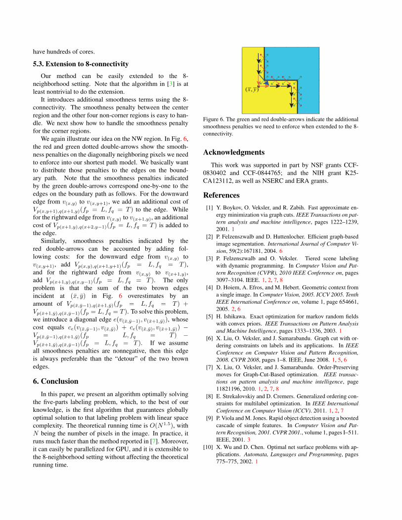
5.3. Extension to 8-connectivity

Our method can be easily extended to the 8-neighborhood setting. Note that the algorithm in [3] is atleast nontrivial to do the extension.

It introduces additional smoothness terms using the 8-connectivity. The smoothness penalty between the centerregion and the other four non-corner regions is easy to han-dle. We next show how to handle the smoothness penaltyfor the corner regions.

We again illustrate our idea on the NW region. In Fig. 6,the red and green dotted double-arrows show the smooth-ness penalties on the diagonally neighboring pixels we needto enforce into our shortest path model. We basically wantto distribute those penalties to the edges on the bound-ary path. Note that the smoothness penalties indicatedby the green double-arrows correspond one-by-one to theedges on the boundary path as follows. For the downwardedge from v(x,y) to v(x,y+1), we add an additional cost ofVp(x,y+1),q(x+1,y)(fp = L, fq = T ) to the edge. Whilefor the rightward edge from v(x,y) to v(x+1,y), an additionalcost of Vp(x+1,y),q(x+2,y−1)(fp = L, fq = T ) is added tothe edge.

Similarly, smoothness penalties indicated by thered double-arrows can be accounted by adding fol-lowing costs: for the downward edge from v(x,y) tov(x,y+1), add Vp(x,y),q(x+1,y+1)(fp = L, fq = T ),and for the rightward edge from v(x,y) to v(x+1,y),add Vp(x+1,y),q(x,y−1)(fp = L, fq = T ). The onlyproblem is that the sum of the two brown edgesincident at (x, y) in Fig. 6 overestimates by anamount of Vp(x,y−1),q(x+1,y)(fp = L, fq = T ) +Vp(x+1,y),q(x,y−1)(fp = L, fq = T ). To solve this problem,we introduce a diagonal edge e(v(x,y−1), v(x+1,y)), whosecost equals ce(v(x,y−1), v(x,y)) + ce(v(x,y), v(x+1,y)) −Vp(x,y−1),q(x+1,y)(fp = L, fq = T ) −Vp(x+1,y),q(x,y−1)(fp = L, fq = T ). If we assumeall smoothness penalties are nonnegative, then this edgeis always preferable than the “detour” of the two brownedges.

6. ConclusionIn this paper, we present an algorithm optimally solving

the five-parts labeling problem, which, to the best of ourknowledge, is the first algorithm that guarantees globallyoptimal solution to that labeling problem with linear spacecomplexity. The theoretical running time is O(N1.5), withN being the number of pixels in the image. In practice, itruns much faster than the method reported in [7]. Moreover,it can easily be parallelized for GPU, and it is extensible tothe 8-neighborhood setting without affecting the theoreticalrunning time.

( , )x y

Figure 6. The green and red double-arrows indicate the additionalsmoothness penalties we need to enforce when extended to the 8-connectivity.

AcknowledgmentsThis work was supported in part by NSF grants CCF-

0830402 and CCF-0844765; and the NIH grant K25-CA123112, as well as NSERC and ERA grants.

References[1] Y. Boykov, O. Veksler, and R. Zabih. Fast approximate en-

ergy minimization via graph cuts. IEEE Transactions on pat-tern analysis and machine intelligence, pages 1222–1239,2001. 1

[2] P. Felzenszwalb and D. Huttenlocher. Efficient graph-basedimage segmentation. International Journal of Computer Vi-sion, 59(2):167181, 2004. 6

[3] P. Felzenszwalb and O. Veksler. Tiered scene labelingwith dynamic programming. In Computer Vision and Pat-tern Recognition (CVPR), 2010 IEEE Conference on, pages3097–3104. IEEE. 1, 2, 7, 8

[4] D. Hoiem, A. Efros, and M. Hebert. Geometric context froma single image. In Computer Vision, 2005. ICCV 2005. TenthIEEE International Conference on, volume 1, page 654661,2005. 2, 6

[5] H. Ishikawa. Exact optimization for markov random fieldswith convex priors. IEEE Transactions on Pattern Analysisand Machine Intelligence, pages 1333–1336, 2003. 1

[6] X. Liu, O. Veksler, and J. Samarabandu. Graph cut with or-dering constraints on labels and its applications. In IEEEConference on Computer Vision and Pattern Recognition,2008. CVPR 2008, pages 1–8. IEEE, June 2008. 1, 5, 6

[7] X. Liu, O. Veksler, and J. Samarabandu. Order-Preservingmoves for Graph-Cut-Based optimization. IEEE transac-tions on pattern analysis and machine intelligence, page11821196, 2010. 1, 2, 7, 8

[8] E. Strekalovskiy and D. Cremers. Generalized ordering con-straints for multilabel optimization. In IEEE InternationalConference on Computer Vision (ICCV). 2011. 1, 2, 7

[9] P. Viola and M. Jones. Rapid object detection using a boostedcascade of simple features. In Computer Vision and Pat-tern Recognition, 2001. CVPR 2001., volume 1, pages I–511.IEEE, 2001. 3

[10] X. Wu and D. Chen. Optimal net surface problems with ap-plications. Automata, Languages and Programming, pages775–775, 2002. 1