Fast and Exact Solution of Total Variation Models on the GPU

Thomas Pock1,2, Markus Unger11Institute for Computer Graphics and Vision, Graz University of Technology

pock, unger, bischof@icg.tugraz.at

Daniel Cremers2 and Horst Bischof12Department of Computer Sience, University of Bonn

pock, dcremers@cs.uni-bonn.de

Abstract

This paper discusses fast and accurate methods to solveTotal Variation (TV) models on the graphics processingunit (GPU). We review two prominent models incorporatingTV regularization and present different algorithms to solvethese models. We mainly concentrate on variational tech-niques, i.e. algorithms which aim at solving the Euler La-grange equations associated with the variational model. Wethen show that particularly these algorithms can be effec-tively accelerated by implementing them on parallel archi-tectures such as GPUs. For comparison we chose a state-of-the-art method based on discrete optimization techniques.We then present the results of a rigorous performance eval-uation including 2D and 3D problems. As a main resultwe show that the our GPU based algorithms clearly out-perform discrete optimization techniques in both speed andmaximum problem size.

1. IntroductionVariational methods are among the most successful

methods to solve a number of inverse problems in Com-puter Vision. Basically, variational methods aim to mini-mize an energy functional which is designed to appropri-ately describe the behavior of a certain Computer Visiontask. The variational approach provides therefore a way toimplement unsupervised processes by simply looking forthe minimizer of the energy functional. Minimization isusually carried out by solving the Euler Lagrange (EL) dif-ferential equation associated with the energy functional.

In particular, variational models incorporating TotalVariation regularization are of great interest for a large classof Computer Vision problems due to its discontinuity pre-serving property. Total Variation methods were introducedfor non-linear image denoising [28] but in the last years theyalso showed great success for a much wider class of Com-

puter Vision problems. Examples include real-time opticalflow computation [34], medical image registration [27], 3Dreconstruction [20], range image fusion [35] and image seg-mentation [30].

Variational optimization techniques are commonly usedto compute the solution of Total Variation models. Due totheir iterative nature they are often considered to be slow,but we show that especially these algorithms can be effec-tively accelerated on streaming processors such as GPUs.This leads to high performance algorithms actually outper-forming state-of-the-art discrete optimization techniques.

The structure of the paper is as follows. In Section 2 wereview two prominent Total Variation models. In Section 3we discuss different algorithms to solve these models. Insection 4 we give details to its numerical implementationon the GPU. Experimental details are presented in Section5. In the last Section we give some conclusions.

2. Total Variation models

The history of L1 estimation procedures goes back toGalileo (1632) and Laplace (1793) and has also received alot of attention from the robust statistics community [19].The first who introduced Total Variation methods to Com-puter Vision tasks were Rudin, Osher and Fatemi (ROF)in their paper on edge preserving image denoising [28].The model is designed to remove noise and other unwantedfine scale details, while preserving sharp discontinuities(edges). The ROF model is defined as the following vari-ational model:

minu

∫Ω

|∇u| dΩ +1

2λ

∫Ω

(u− f)2dΩ, (1)

where Ω is the image domain, f is the observed image func-tion which is assumed to be corrupted by Gaussian noise,and u is the sought solution. The free parameter λ is usedto control the amount of smoothing in u. The aim of the

1

ROF model to minimize the Total Variation of u:∫Ω

|∇u| dΩ =∫

Ω

√(∂u

∂x

)2

+(∂u

∂y

)2

dΩ . (2)

Its main property is that it allows for sharp discontinuitiesin the solution while still being a convex in u [28].

Similar to the ROF model, the TV-L1

model [2], [23], [11] is defined as the variational problem

minu

∫Ω

|∇u| dΩ + λ

∫Ω

|u− f | dΩ. (3)

The difference compared to the ROF model is that thesquared L2 data fidelity term has been replaced by the L1

norm. Moreover, while the ROF model in its unconstrainedformulation (1) poses a strictly convex minimization prob-lem, the TV-L1 model is not strictly convex. This meansthat in general, there is no unique global minimizer.

The TV-L1 model also offers some desirable improve-ments. First, it turns out that the TV-L1 model is more ef-fective than the ROF model in removing impulse noise (e.g.salt and pepper noise) [23]. Second, the TV-L1 model iscontrast invariant. This means that, if u is a solution of (3)for a certain input image f , then cu is also a solution forcf for c ∈ R+. Therefore the TV-L1 model has a stronggeometrical meaning which makes it useful for scale-drivenfeature selection [13] and denoising of shapes [24].

3. Computing the Solution of Total Variationmodels

AlgorithmsExplicit time marching [28], [21]

Linearization of the EL equation [32], [31], [8]Nonlinear primal-dual method [12]

Duality based methods [12], [6], [5], [18], [7], [22]Non-linear multigrid methods [15], [4], [29], [10], [9]

First order schemes from convex optimization [33]Second-order cone programming [16]

Graph cut methods [14], [7], [17]Table 1. A selected list of numerical algorithms to solve Total Vari-ation models.

Computing the solution of Total Variation models isa challenging task. The main reason lies in the non-differentiability of the L1 norm at zero. It is therefore notsurprising that one can find many items about this topic inthe literature. Tab. 1 gives a selected overview of numeri-cal methods to solve Total Variation models. Describing allthese approaches in detail is clearly beyond the scope of thispaper. We rather proceed by restricting our investigations tothe variational approach. We do this mainly for three rea-sons. First, variational methods are very general and can

easily be adapted to different applications. Second, varia-tional algorithms provide a continuous solution to the un-derlying optimization problem. Third, variational methodsare well suited to be computed on highly parallel computerarchitectures such as graphics processing units (GPUs).

3.1. Computing the Solution of the ROF Model

The aim of the variational approach is to minimize anenergy functional by solving its associated Euler-Lagrange(EL) differential equation. For the unconstrained ROFmodel the EL equation is given by

−∇ ·(∇u|∇u|

)+

1λ

(u− f) = 0 , (4)

When looking at this equation, one can make two obser-vations: First, due to the 1

|∇u| term, the equation is highlynon-linear. Second, the equation is not defined for∇u = 0.To overcome the second limitation, a simple and commonlyused approach is to replace |∇u| by a regularized version|∇u|ε =

√|∇u|2 + ε. However, for small ε the equation

is still nearly degenerated and for larger ε the ability of theROF model to preserve sharp discontinuities is lost.

In [32], Vogel and Oman proposed a fixed point algo-rithm to solve (4). The basic idea is to linearize (4) by tak-ing the non-linear terms 1

|∇u| εfrom the previous iteration.

Therefore, at each iteration n, their method requires to solvea sparse system of linear equations

−∇(∇un+1

|∇un|ε

)+

1λ

(un+1 − f

)= 0 . (5)

This can be done with any sparse solver (e.g. Jacobi, Gauss-Seidel, SOR). In practice, the system of linear equationsneeds not to be solved exactly during each iteration. A fewiterations of a Jacobi or Gauss-Seidel algorithm are suffi-cient to achieve a reasonable convergence of the entire al-gorithm. One serious limitation of this method is still thechoice of the regularization parameter ε. Again, for smallε the algorithm becomes slow in flat regions and for largeε edges get blurred. We will refer to this algorithm in thefollowing as ROF-primal.

Chan et al. in [12], Carter et al. in [5] and Chambollein [6] studied the dual formulation of the ROF model. Allthree approaches exploit the dual formulation of the TVnorm:

|∇u| = maxpp · ∇u : ‖p‖ ≤ 1 . (6)

By substituting this expression into the ROF model (1) onearrives at the so-called primal-dual formulation of the ROFmodel

minu

max‖p‖≤1

∫Ω

p · ∇u dΩ +1

2λ

∫Ω

(u− f)2dΩ. (7)

Since this expression is convex, we can interchange the minand the max. Furthermore, the optimality condition withrespect to u is readily given by

u = f + λ∇ · p . (8)

Using this relation, the primal variable u can be eliminatedand one arrives at the dual ROF model

min‖p‖≤1

−∫

Ω

p · ∇f dΩ +λ

2

∫Ω

(∇ · p)2dΩ. (9)

Note that in order to be consistent with the other ap-proaches, we have turned the original maximization prob-lem with respect to the dual variable (see (7)) into a mini-mization problem. We do this by flipping the sign of the en-tire functional. The Euler-Lagrange equation of (9) is givenby

−∇ (f + λ∇ · p) = 0 , ‖p‖ ≤ 1 . (10)

The major advantage of the dual ROF model is that it is con-tinuously differentiable and therefore does not suffer fromthe problem of the primal model which gets degeneratedif ∇u = 0. On the other hand, the dual problem has theconstraint that ‖p‖ ≤ 1, which requires sophisticated op-timization techniques. In [5], Carter studied several algo-rithms (interior-point primal-dual method with three relax-ation methods: dual, hybrid, and barrier) to solve the dualROF model. However, the algorithms are not very useful forpractical problems due to a heavy runtimes and dependenceon additional parameters.

It is somehow astonishing that there exists a very ba-sic algorithm which has not been considered by Carterin [5]. In fact, a simple but efficient algorithm is obtainedby a straightforward gradient descent and subsequent re-projection of (10).

pn+1 =pn + τ

λ (∇ (f + λ∇ · pn))max(1,

∣∣pn + τλ (∇ (f + λ∇ · pn))

∣∣ . (11)

This algorithm has been proposed by Chambolle in [7] as avariant of a more comprehensive algorithm [6]. In practice,convergence is achieved as long as τ ≤ 1/4. The primalvariable can be recovered via u = f + λ∇ · p. Besides itssimplicity, a further promise of this algorithm is its robust-ness an a fast convergence. We will refer to this algorithmin the following as ROF-dual.

Very recently, Aujol [1] established connections betweenthe projected gradient descend algorithm [7], and a classof more general algorithms proposed almost 30 years agoin [3].

3.2. Computing the Solution of the TV-L1 Model

Unfortunately, the TV-L1 model (3) makes use of twoL1

norms, one for the TV term and one for data term. Therefore

the TV-L1 model is not strictly convex meaning that manysolutions may exist. This gives us raise to the assumptionthat the TV-L1 model is even more difficult to solve thanthe ROF model. Let us take a look at the Euler-Lagrangeequation of the TV-L1 model:

−∇ ·(∇u|∇u|

)+ λ

(u− f)|u− f |

= 0 . (12)

We can easily see that this equation is degenerated eitherif ∇u = 0 or u − f = 0. Therefore a first idea isto apply the same trick we used to regularize the Euler-Lagrange equation of the ROF model. Doing so, we sim-ply replace |∇u| by |∇u|ε =

√|∇u|+ ε and |u − f | by

|u− f |δ =√|u− f |2 + δ.

To find a convergent algorithm to solve the regularizedEuler-Lagrange equation, we follow the approach of Vogeland Oman. For each iteration n + 1 we have to solve thefollowing sparse system of linear equations:

−∇ ·(∇un+1

|∇un|ε

)+ λ

(un+1 − f)|un − f |δ

= 0 , (13)

where the non-linear terms have been taken from the previ-ous iteration n. We note that the performance of this algo-rithm is very sensitive with respect to the particular choiceof the parameters ε and δ. Basically, small values of ε and δslow down the algorithm a lot and large values of ε and δ in-duce large errors with respect to the original TV-L1 model.We will refer to this algorithm in the following as TVL1-primal.

A natural question is, whether we can solve the TV-L1

model exactly? More precisely, can we make use of thesame duality principles, we used to solve the ROF modelexactly? Unfortunately, it turns out that we cannot use theduality principles directly. The reason is that the TV-L1

model is not strictly convex.In order to make the TV-L1 model strictly convex, Aujol

et al. proposed the following convex approximation [2]:

minu,v

∫Ω

|∇u|dΩ +12θ

∫Ω

(u− v)2dΩ + λ

∫Ω

|v − f |dΩ.

(14)For θ > 0 (14) is a convex approximation of the TV-L1

model and as θ → 0 (14) approaches the original TV-L1

model (3).Unlike the original TV-L1 model (14) is now a optimiza-

tion problem in two variables, u and v. Therefore we haveto perform an alternating minimization with respect to u andv. The outline of the alternating minimization procedure isas follows:

1. For fixed v, solve (14) for u.

minu

∫Ω

|∇u| dΩ +12θ

∫Ω

(u− v)2dΩ. (15)

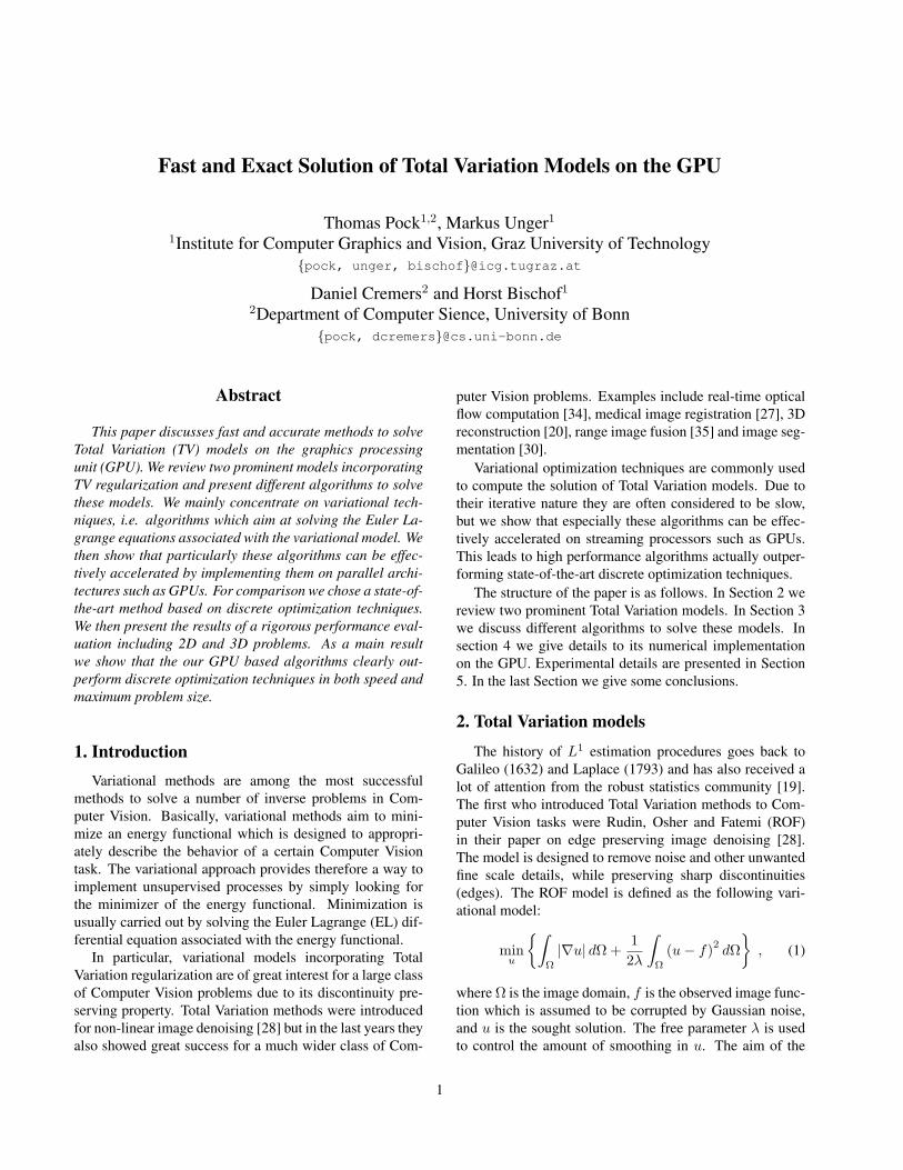
(a) (b) (c)

Figure 1. (a, b) Convergence time for the ROF and TV-L1 algorithms in dependence of number of internal iterations. (c) Overall iterationsper second in depenence of number of internal iterations.

This optimization problem is exactly the ROF model,with θ being the regularization parameter. We can usethe projected gradient descend algorithm to solve thissub-problem.

2. For fixed u, solve (14) for v.

minv

12θ

∫Ω

(u− v)2dΩ + λ

∫Ω

|v − f |dΩ. (16)

(16) is a point-wise convex minimization prob-lem which can be solved via the following soft-thresholding scheme:

v =

u− λθ if u− f > λθu+ λθ if u− f < −λθf if |u− f | ≤ λθ

(17)

3. Goto 1. until convergence.

We note that the algorithm is very robust with respect to thechoice of the approximation parameter θ. We found thata good choice is to set θ such that the soft-threshold λθ is1 − 5% of the maximum gray-level interval of f . We willrefer to this algorithm in the following as TVL1-dual.

4. Implementation on the GPU using CUDAWe implemented the following variational variational al-

gorithms: ROF-primal, ROF-dual, TVL1-primal and TVL1-dual on the graphics card. The implementation is basically astraight-forward implementation of the presented schemes.We used Jacobi’s method to solve the systems of linearequations in the primal methods. Our implementations canhandle 2D and 3D problems.

With the introduction of the 8-series [25], NVidia alsointroduced the CUDA (Compute Unified Device Architec-ture) framework [26]. CUDA provides a standard C lan-guage interface for programming on the GPU. It can handle

a massive number of parallel threads that are scheduled tothe processor. CUDA also provides the user with a pro-gramming interface that handles scheduling and executionon the GPU.

The processing units of the GPU are arranged intogroups of so-called multiprocessors. One multiprocessor,can execute several independent threads having access tothe same shared memory. While reading data from theglobal GPU memory is still fast (about 50 − 100 GB/s),reading from the shared memory is even 75 times faster. Weexploited this feature by loading a local image patch into theshared memory and ran the algorithms for several iterationsbefore writing the results back into global memory. Highspeedups can be gained using the shared memory. On theother hand, the number of such internal iterations shouldalso be limited. The information at block borders cannot beexchanged during computation leading to a slower conver-gence of the entire algorithm. The effects of internal itera-tions versus the convergence behavior the algorithms are il-lustrated in Fig. 1 shows the performance of our algorithmsdepending on the number of internal iterations. We foundthat using 5 internal iterations gives the best overall perfor-mance.

5. Experimental Results

For evaluation we used a standard personal computerequipped with a 2.13 GHz Core2-Duo CPU, 2 GB of mainmemory and a NVidia 8800GTX graphics card. The com-puter runs a 32-bit Linux operating system. Basically, withour GPU based implementation we achieved a speedup fac-tor of approximately 1000 compared to an optimized Mat-lab implementation. However, in this paper we do not com-pare our GPU-based algorithms to CPU-based variants, be-cause this question is of minor interest. The more inter-esting question is weather GPU-accelerated Total Variation

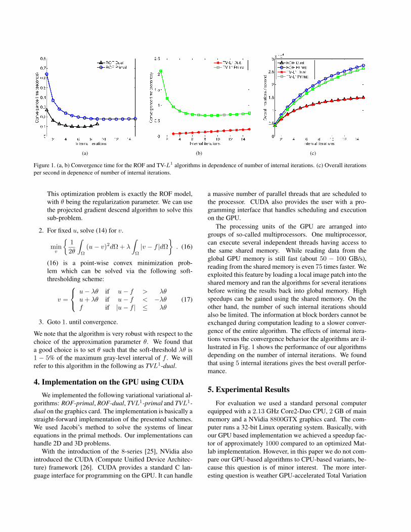
(a) (b) (c) (d) (e)

Figure 2. Test images: (a) Summit image: 256 × 256. (b) Basecamp image: 512 × 512. (c) Sunset image: 1024 × 1024. (d) Brain dataset: 256× 320× 256 . (e) Liver data set: 512× 512× 128

methods can compete with discrete optimization techniquessuch as graph cuts. Note that TV models and graph cuts cansolve problems of equal complexity. So far, it is not clearwhich method will be the clear winner. Maybe, the workpresented in this paper can shed further light on this ques-tion. We therefore decided to compare our algorithms to arecently published method based on parametric max-flowalgorithms [17]. The algorithm of [17] was downloadedfrom Wotao Yin’s homepage. It was executed on the samemachine as the GPU-based algorithms using Matlab 7.0.3.Note that the core of this algorithm is based on a high per-formance C/C++ implementation.

Unfortunately, there exist no sharp L2, or even bet-ter, L∞ error bound for variational methods. A commonmethod is to compute the residuum norm of the Euler-Lagrange equations and to stop the iterations when theresiduum norm is below a certain threshold. On the otherhand, the residual norm does not give any information aboutthe error of the solution with respect to the true solution.Note that graph-cut based algorithms come along with suchan error bound [7], [17]. This is can be seen as a clearadvantage of graph cut methods over variational methods.We applied the following procedure to estimate the L2 er-ror bound. We first run our algorithms for a long time toproduce a ground truth. We can then measure the time thealgorithms need to fall below a predefined L2 error bound.

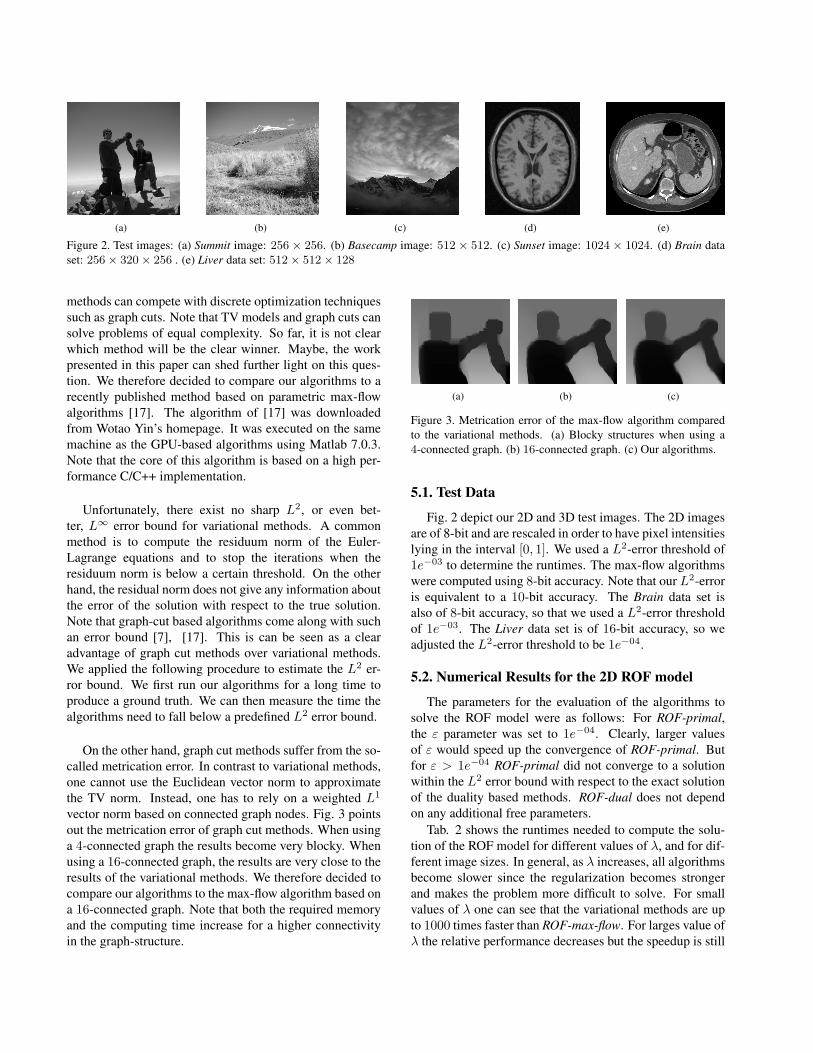
On the other hand, graph cut methods suffer from the so-called metrication error. In contrast to variational methods,one cannot use the Euclidean vector norm to approximatethe TV norm. Instead, one has to rely on a weighted L1

vector norm based on connected graph nodes. Fig. 3 pointsout the metrication error of graph cut methods. When usinga 4-connected graph the results become very blocky. Whenusing a 16-connected graph, the results are very close to theresults of the variational methods. We therefore decided tocompare our algorithms to the max-flow algorithm based ona 16-connected graph. Note that both the required memoryand the computing time increase for a higher connectivityin the graph-structure.

(a) (b) (c)

Figure 3. Metrication error of the max-flow algorithm comparedto the variational methods. (a) Blocky structures when using a4-connected graph. (b) 16-connected graph. (c) Our algorithms.

5.1. Test Data

Fig. 2 depict our 2D and 3D test images. The 2D imagesare of 8-bit and are rescaled in order to have pixel intensitieslying in the interval [0, 1]. We used a L2-error threshold of1e−03 to determine the runtimes. The max-flow algorithmswere computed using 8-bit accuracy. Note that our L2-erroris equivalent to a 10-bit accuracy. The Brain data set isalso of 8-bit accuracy, so that we used a L2-error thresholdof 1e−03. The Liver data set is of 16-bit accuracy, so weadjusted the L2-error threshold to be 1e−04.

5.2. Numerical Results for the 2D ROF model

The parameters for the evaluation of the algorithms tosolve the ROF model were as follows: For ROF-primal,the ε parameter was set to 1e−04. Clearly, larger valuesof ε would speed up the convergence of ROF-primal. Butfor ε > 1e−04 ROF-primal did not converge to a solutionwithin the L2 error bound with respect to the exact solutionof the duality based methods. ROF-dual does not dependon any additional free parameters.

Tab. 2 shows the runtimes needed to compute the solu-tion of the ROF model for different values of λ, and for dif-ferent image sizes. In general, as λ increases, all algorithmsbecome slower since the regularization becomes strongerand makes the problem more difficult to solve. For smallvalues of λ one can see that the variational methods are upto 1000 times faster than ROF-max-flow. For larges value ofλ the relative performance decreases but the speedup is still

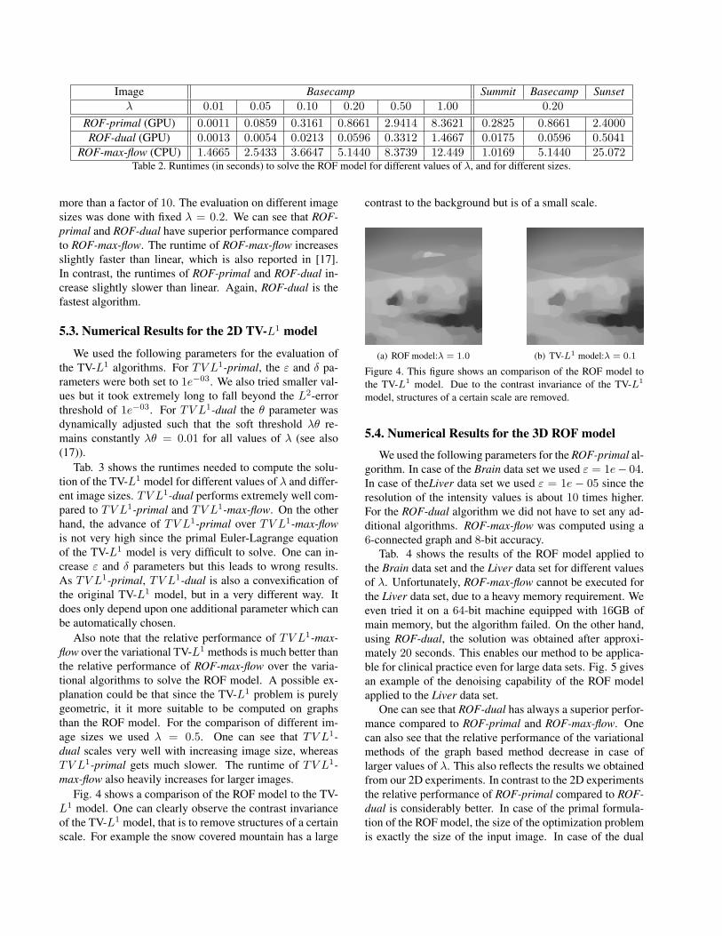
Image Basecamp Summit Basecamp Sunsetλ 0.01 0.05 0.10 0.20 0.50 1.00 0.20

ROF-primal (GPU) 0.0011 0.0859 0.3161 0.8661 2.9414 8.3621 0.2825 0.8661 2.4000ROF-dual (GPU) 0.0013 0.0054 0.0213 0.0596 0.3312 1.4667 0.0175 0.0596 0.5041

ROF-max-flow (CPU) 1.4665 2.5433 3.6647 5.1440 8.3739 12.449 1.0169 5.1440 25.072Table 2. Runtimes (in seconds) to solve the ROF model for different values of λ, and for different sizes.

more than a factor of 10. The evaluation on different imagesizes was done with fixed λ = 0.2. We can see that ROF-primal and ROF-dual have superior performance comparedto ROF-max-flow. The runtime of ROF-max-flow increasesslightly faster than linear, which is also reported in [17].In contrast, the runtimes of ROF-primal and ROF-dual in-crease slightly slower than linear. Again, ROF-dual is thefastest algorithm.

5.3. Numerical Results for the 2D TV-L1 model

We used the following parameters for the evaluation ofthe TV-L1 algorithms. For TV L1-primal, the ε and δ pa-rameters were both set to 1e−03. We also tried smaller val-ues but it took extremely long to fall beyond the L2-errorthreshold of 1e−03. For TV L1-dual the θ parameter wasdynamically adjusted such that the soft threshold λθ re-mains constantly λθ = 0.01 for all values of λ (see also(17)).

Tab. 3 shows the runtimes needed to compute the solu-tion of the TV-L1 model for different values of λ and differ-ent image sizes. TV L1-dual performs extremely well com-pared to TV L1-primal and TV L1-max-flow. On the otherhand, the advance of TV L1-primal over TV L1-max-flowis not very high since the primal Euler-Lagrange equationof the TV-L1 model is very difficult to solve. One can in-crease ε and δ parameters but this leads to wrong results.As TV L1-primal, TV L1-dual is also a convexification ofthe original TV-L1 model, but in a very different way. Itdoes only depend upon one additional parameter which canbe automatically chosen.

Also note that the relative performance of TV L1-max-flow over the variational TV-L1 methods is much better thanthe relative performance of ROF-max-flow over the varia-tional algorithms to solve the ROF model. A possible ex-planation could be that since the TV-L1 problem is purelygeometric, it it more suitable to be computed on graphsthan the ROF model. For the comparison of different im-age sizes we used λ = 0.5. One can see that TV L1-dual scales very well with increasing image size, whereasTV L1-primal gets much slower. The runtime of TV L1-max-flow also heavily increases for larger images.

Fig. 4 shows a comparison of the ROF model to the TV-L1 model. One can clearly observe the contrast invarianceof the TV-L1 model, that is to remove structures of a certainscale. For example the snow covered mountain has a large

contrast to the background but is of a small scale.

(a) ROF model:λ = 1.0 (b) TV-L1 model:λ = 0.1

Figure 4. This figure shows an comparison of the ROF model tothe TV-L1 model. Due to the contrast invariance of the TV-L1

model, structures of a certain scale are removed.

5.4. Numerical Results for the 3D ROF model

We used the following parameters for the ROF-primal al-gorithm. In case of the Brain data set we used ε = 1e− 04.In case of theLiver data set we used ε = 1e − 05 since theresolution of the intensity values is about 10 times higher.For the ROF-dual algorithm we did not have to set any ad-ditional algorithms. ROF-max-flow was computed using a6-connected graph and 8-bit accuracy.

Tab. 4 shows the results of the ROF model applied tothe Brain data set and the Liver data set for different valuesof λ. Unfortunately, ROF-max-flow cannot be executed forthe Liver data set, due to a heavy memory requirement. Weeven tried it on a 64-bit machine equipped with 16GB ofmain memory, but the algorithm failed. On the other hand,using ROF-dual, the solution was obtained after approxi-mately 20 seconds. This enables our method to be applica-ble for clinical practice even for large data sets. Fig. 5 givesan example of the denoising capability of the ROF modelapplied to the Liver data set.

One can see that ROF-dual has always a superior perfor-mance compared to ROF-primal and ROF-max-flow. Onecan also see that the relative performance of the variationalmethods of the graph based method decrease in case oflarger values of λ. This also reflects the results we obtainedfrom our 2D experiments. In contrast to the 2D experimentsthe relative performance of ROF-primal compared to ROF-dual is considerably better. In case of the primal formula-tion of the ROF model, the size of the optimization problemis exactly the size of the input image. In case of the dual

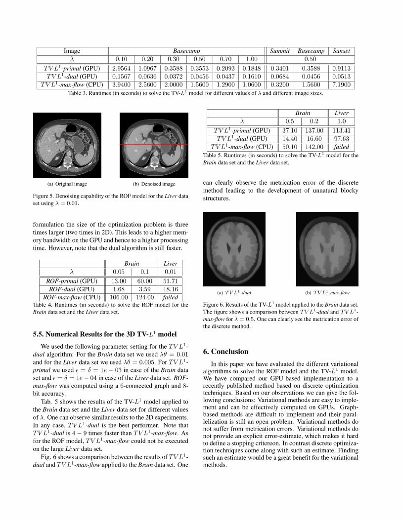
Image Basecamp Summit Basecamp Sunsetλ 0.10 0.20 0.30 0.50 0.70 1.00 0.50

TV L1-primal (GPU) 2.9564 1.0967 0.3588 0.3553 0.2093 0.1848 0.3401 0.3588 0.9113TV L1-dual (GPU) 0.1567 0.0636 0.0372 0.0456 0.0437 0.1610 0.0684 0.0456 0.0513

TV L1-max-flow (CPU) 3.9400 2.5600 2.0000 1.5600 1.2900 1.0600 0.3200 1.5600 7.1900Table 3. Runtimes (in seconds) to solve the TV-L1 model for different values of λ and different image sizes.

(a) Original image (b) Denoised image

Figure 5. Denoising capability of the ROF model for the Liver dataset using λ = 0.01.

formulation the size of the optimization problem is threetimes larger (two times in 2D). This leads to a higher mem-ory bandwidth on the GPU and hence to a higher processingtime. However, note that the dual algorithm is still faster.

Brain Liverλ 0.05 0.1 0.01

ROF-primal (GPU) 13.00 60.00 51.71ROF-dual (GPU) 1.68 3.59 18.16

ROF-max-flow (CPU) 106.00 124.00 failedTable 4. Runtimes (in seconds) to solve the ROF model for theBrain data set and the Liver data set.

5.5. Numerical Results for the 3D TV-L1 model

We used the following parameter setting for the TV L1-dual algorithm: For the Brain data set we used λθ = 0.01and for the Liver data set we used λθ = 0.005. For TV L1-primal we used ε = δ = 1e − 03 in case of the Brain dataset and ε = δ = 1e− 04 in case of the Liver data set. ROF-max-flow was computed using a 6-connected graph and 8-bit accuracy.

Tab. 5 shows the results of the TV-L1 model applied tothe Brain data set and the Liver data set for different valuesof λ. One can observe similar results to the 2D experiments.In any case, TV L1-dual is the best performer. Note thatTV L1-dual is 4− 9 times faster than TV L1-max-flow. Asfor the ROF model, TV L1-max-flow could not be executedon the large Liver data set.

Fig. 6 shows a comparison between the results of TV L1-dual and TV L1-max-flow applied to the Brain data set. One

Brain Liverλ 0.5 0.2 1.0

TV L1-primal (GPU) 37.10 137.00 113.41TV L1-dual (GPU) 14.40 16.60 97.63

TV L1-max-flow (CPU) 50.10 142.00 failedTable 5. Runtimes (in seconds) to solve the TV-L1 model for theBrain data set and the Liver data set.

can clearly observe the metrication error of the discretemethod leading to the development of unnatural blockystructures.

(a) TV L1-dual (b) TV L1-max-flow

Figure 6. Results of the TV-L1 model applied to the Brain data set.The figure shows a comparison between TV L1-dual and TV L1-max-flow for λ = 0.5. One can clearly see the metrication error ofthe discrete method.

6. ConclusionIn this paper we have evaluated the different variational

algorithms to solve the ROF model and the TV-L1 model.We have compared our GPU-based implementation to arecently published method based on discrete optimizationtechniques. Based on our observations we can give the fol-lowing conclusions: Variational methods are easy to imple-ment and can be effectively computed on GPUs. Graph-based methods are difficult to implement and their paral-lelization is still an open problem. Variational methods donot suffer from metrication errors. Variational methods donot provide an explicit error-estimate, which makes it hardto define a stopping critereon. In contrast discrete optimiza-tion techniques come along with such an estimate. Findingsuch an estimate would be a great benefit for the variationalmethods.

References[1] J.-F. Aujol. Some algorithms for total variation based im-

age restoration. Technical report, CMLA, ENS CACHAN,CNRS, UNIVERSUD, 2008.

[2] J.-F. Aujol, G. Gilboa, T. Chan, and S. Osher. Structure-texture image decomposition–modeling, algorithms, and pa-rameter selection. Int. J. Comp. Vis., 67(1):111–136, 2006.

[3] A. Bermudez and C. Moreno. Duality methods for solvingvariational inequalities. Comp. and Math. with Appls., 7:43–58, 1981.

[4] A. Bruhn and J. Weickert. Towards ultimate motion esti-mation: Combining highest accuracy with real-time perfor-mance. In Proc. 11th Int. Conf. Comp. Vis., pages 749–755,2005.

[5] J. Carter. Dual Methods for Total Variation-based ImageRestoration. PhD thesis, UCLA, Los Angeles, CA, 2001.

[6] A. Chambolle. An algorithm for total variation minimiza-tions and applications. J. Math. Imaging Vis., 2004.

[7] A. Chambolle. Total variation minimization and a class ofbinary MRF models. In Energy Minimization Methods inComputer Vision and Pattern Recognition, pages 136–152,2005.

[8] A. Chambolle and P.-L. Lions. Image recovery via totalvariation minimization and related problems. Numer. Math.,76:167–188, 1997.

[9] T. Chan and K. Chen. On a nonlinear multigrid algorithmwith primal relaxation for the image total variation minimi-sation. Numerical Algorithms, 41:387–411, 2006.

[10] T. Chan, K. Chen, and J. Carter. Iterative methods forsolving the dual formulation arising from image restoration.Electronic Transactions on Numerical Analysis, 26:299–311,2007.

[11] T. Chan and S. Esedoglu. Aspects of total variation regu-larized L1 function approximation. SIAM J. Appl. Math.,65(5):1817–1837, 2004.

[12] T. Chan, G. Golub, and P. Mulet. A nonlinear primal-dualmethod for total variation-based image restoration. SIAM J.Sci. Comp., 20(6):1964–1977, 1999.

[13] T. Chen, W. Yin, X. Zhou, D. Comaniciu, and T. Huang.Total variation models for variable lighting face recognition.IEEE Trans. Pattern Anal. Mach. Intell., 28(9):1519–1524,2006.

[14] J. Darbon and M. Sigelle. Image restoration with discreteconstrained total variation, part i: fast and exact optimiza-tion. J. Math. Imaging Vis., 26(3):261–276, 2006.

[15] C. Frohn-Schauf, S. Henn, and K. Witsch. Nonlinear multi-grid methods for total variation image denoising. Comput.Visual Sci., pages 199–206, 2004.

[16] D. Goldfarb and W. Yin. Second-order cone programmingmethods for total variation-based image restoration. SIAMJournal on Scientific Computing, 27(2):622–645, 2005.

[17] D. Goldfarb and W. Yin. Parametric maximum flow algo-rithms for fast total variation minimization. Technical report,Rice University, 2007.

[18] M. Hintermuller and K. Kunisch. Total bounded variationregularization as bilaterally constrained optimization prob-lems. SIAP, 64(4):1311–1333, 2004.

[19] P. Huber. Robust Statistics. Wiley, New York, 1981.[20] K. Kolev, M. Klodt, T. Brox, S. Esedoglu, and D. Cremers.

Continuous global optimization in multiview 3D reconstruc-tion. In Energy Minimization Methods in Computer Visionand Pattern Recognition, pages 441–452, China, 2007.

[21] A. Marquina and S. Osher. Explicit algorithms for a newtime dependent model based on level set motion for nonlin-ear deblurring and noise removal. SIAM J. Sci. Comput.,22:387–405, 2000.

[22] M. K. Ng, L. Qi, Y.-F. Yang, and Y.-M. Huang. On semis-mooth Newton’s method for total variation minimization. J.Math. Imaging Vis., 27:265–276, 2007.

[23] M. Nikolova. A variational approach to remove outliers andimpulse noise. J. Math. Imaging Vis., 20(1-2):99–120, 2004.

[24] M. Nikolova, S. Esedoglu, and T. Chan. Algorithms for find-ing global minimizers of image segmentation and denoisingmodels. SIAM Journal of Applied Mathematics, 66(5):1632–1648, 2006.

[25] NVidia. NVidia GeForce 8800 GPU architecture overview.Technical report, NVidia, 2006.

[26] NVidia. Nvidia CUDA Compute Unified Device Architec-ture programming guide 1.1. Technical report, NVidia, 2007.

[27] T. Pock, M. Urschler, C. Zach, R. Beichel, and H. Bischof. Aduality based algorithm for TV-L1-optical-flow image regis-tration. In 10th International Conference on Medical ImageComputing and Computer Assisted Intervention, pages 511–518, Brisbane, Australia, 2007.

[28] L. Rudin, S. Osher, and E. Fatemi. Nonlinear total variationbased noise removal algorithms. Physica D, 60:259–268,1992.

[29] J. Savage and K. Chen. An improved and accelerated nonlin-ear multigrid method for total-variation denoising. J. Math.Imaging Vis., 82(8):1001–1015, 2005.

[30] M. Unger, T. Pock, and H. Bischof. Continuous globallyoptimal image segmentation with local constraints. In Com-puter Vision Winter Workshop 2008, page accepted, 2008.

[31] C. Vogel. A multigrid method for total variation-based imagedenoising. Progress in Systems and Control Theory, 1995.

[32] C. Vogel and M. Oman. Iteration methods for total variationdenoising. SIAM J. Sci. Comp., 17:227–238, 1996.

[33] P. Weiss, L. Blanc-Feraud, and G. Aubert. Efficient schemesfor total variation minimization under constraints in imageprocessing. Technical report, INRIA, 2007.

[34] C. Zach, T. Pock, and H. Bischof. A duality based approachfor realtime TV-L1 optical flow. In 29th DAGM Symposiumon Pattern Recognition, pages 214–223, Heidelberg, Ger-many, 2007.

[35] C. Zach, T. Pock, and H. Bischof. A globally optimal al-gorithm for robust TV-L1 range image integration. In Proc.13th Int. Conf. Comp. Vis., Rio de Janeiro, Brazil, 2007.