farm employment transitions: a markov …ageconsearch.umn.edu/bitstream/21353/1/sp06iw01.pdf ·...

FARM EMPLOYMENT TRANSITIONS: A MARKOV CHAIN ANALYSIS WITH SELF-SELECTIVITY

Nobuyuki Iwai International Agricultural Trade & Policy Center

Food and Resource Economics Department PO Box 110240, University of Florida

Gainesville, FL 32611 [email protected]

Robert D. Emerson International Agricultural Trade & Policy Center

Food and Resource Economics Department PO Box 110240, University of Florida


Lurleen M. Walters International Agricultural Trade & Policy Center

Food and Resource Economics Department P.O. Box 110240, University of Florida


Selected Paper prepared for presentation at the American Agricultural Economics Association Annual Meeting, Long Beach, California, July 23-26, 2006.

Copyright 2006 by Nobuyuki Iwai, Robert D. Emerson, and Lurleen M. Walters. All rights reserved. Readers may make verbatim copies of this document for non-commercial purposes by

any means, provided that this copyright notice appears on all such copies.

mailto:[email protected]

FARM EMPLOYMENT TRANSITIONS: A MARKOV CHAIN ANALYSIS WITH SELF-SELECTIVITY*

Introduction

The U.S. agricultural labor market is heavily dependent on foreign-born workers.

According to the 2002 National Agricultural Workers Survey (NAWS) report, 77 percent

of agricultural workers were foreign-born for the years 2001-02 (Carroll et al. 2005).

Approximately 69 percent of these foreign-born workers lacked authorization to work in

the U.S. Hence, 53 percent of all farm workers were undocumented for the same period

(Carroll et al. 2005), making U.S. agriculture one of the most undocumented-worker-

intensive industries.

Political and national interest in immigration reform rose sharply over the last few

years, resulting in the introduction of two bills – somewhat diametrically opposed – in the

109th U.S. Congress. For example, in December 2005 the U.S. House of Representatives

passed H.R. 4437 which is considerably stricter on enforcement than the recent Senate

immigration bill (S. 2611) which favors legalization and guest worker programs for

undocumented immigrant workers1. Given the high proportion of unauthorized workers

in the agricultural labor force, farm employers are concerned that labor availability and

* The authors are grateful to Susan Gabbard, Trish Hernandez, Alberto Sandoval and their associates at Aguirre International for assistance with the NAWS data, and to Daniel Carroll at the U.S. Department of Labor for granting access and authorization to use the NAWS data. This research has been supported through a partnership agreement with the Risk Management Agency, U.S. Department of Agriculture; by the Center for International Business Education and Research at the University of Florida; and by the Florida Agricultural Experiment Station. The authors alone are responsible for any views expressed in the paper. 1 HR. 4437 (the Border Protection, Antiterrorism & Illegal Immigration Act of 2005) and the S. 2611 (Comprehensive Immigration Reform Act of 2006) disagree sharply on how undocumented immigrants should be dealt with by law.

1

cost may be adversely affected if certain reforms are passed, and specifically if they are

more stringently applied across the board (Walters et al. 2006).

Not surprisingly, the debate that has ensued on immigration reform and its

implications for agriculture is quite similar to that which preceded the passage of the

Immigration Reform and Control Act (IRCA) in 1986. In order to discourage the

employment of unauthorized immigrant labor in the U.S, several measures were

implemented. These included employer sanctions, a supplemental guest worker program,

modification of the H-2 program, and legalization of unauthorized workers.

Approximately 1.3 million unauthorized farm workers were granted legal status and

many farmers and politicians were concerned about the effect on U.S. agriculture. Their

prediction was that undocumented agricultural workers who received amnesty would

leave agriculture for other employment opportunities, and this would lead to serious labor

shortages and wage increases in US agriculture (Tran and Perloff 2002). These

predictions did not materialize since the employment of unauthorized workers in U.S.

agriculture has increased over time. This increase in undocumented workers seems to

suggest that IRCA has not been as effective as lawmakers had intended2.

However, there is no generally-accepted interpretation on why this considerable

increase in composition of unauthorized workers occurred in U.S. agriculture after the

IRCA. This phenomenon is even puzzling since existing literature generally concludes

that legal status tends to lengthen the duration of a worker staying in farm work. There

are two representative methods in the empirical study of the relationship between legal

2 The proportion of unauthorized workers in U.S. agriculture has risen from 7% in 1989 to 32% for the years 1994-95, and 53% in 2001-02 (Mines et al. 1997, Carroll et al. 2005).

2

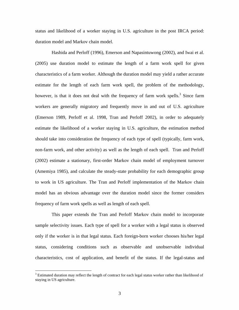
status and likelihood of a worker staying in U.S. agriculture in the post IRCA period:

duration model and Markov chain model.

Hashida and Perloff (1996), Emerson and Napasintuwong (2002), and Iwai et al.

(2005) use duration model to estimate the length of a farm work spell for given

characteristics of a farm worker. Although the duration model may yield a rather accurate

estimate for the length of each farm work spell, the problem of the methodology,

however, is that it does not deal with the frequency of farm work spells.3 Since farm

workers are generally migratory and frequently move in and out of U.S. agriculture

(Emerson 1989, Perloff et al. 1998, Tran and Perloff 2002), in order to adequately

estimate the likelihood of a worker staying in U.S. agriculture, the estimation method

should take into consideration the frequency of each type of spell (typically, farm work,

non-farm work, and other activity) as well as the length of each spell. Tran and Perloff

(2002) estimate a stationary, first-order Markov chain model of employment turnover

(Amemiya 1985), and calculate the steady-state probability for each demographic group

to work in US agriculture. The Tran and Perloff implementation of the Markov chain

model has an obvious advantage over the duration model since the former considers

frequency of farm work spells as well as length of each spell.

This paper extends the Tran and Perloff Markov chain model to incorporate

sample selectivity issues. Each type of spell for a worker with a legal status is observed

only if the worker is in that legal status. Each foreign-born worker chooses his/her legal

status, considering conditions such as observable and unobservable individual

characteristics, cost of application, and benefit of the status. If the legal-status and

3 Estimated duration may reflect the length of contract for each legal status worker rather than likelihood of staying in US agriculture.

3

employment-status selection are correlated, the Markov chain model may yield biased

estimators without correcting for the legal-status selection process. Regarding this, both

Hashida and Perloff (1996) and Iwai et al. (2005) point out the serious sample selection

bias problem in their duration models.4 In order to compensate for the problems in the

two representative methods above, it may be necessary to develop and estimate a Markov

chain model with correction for sample selection bias.

We have the following three objectives in the current study. We propose a

stationary, first-order Markov chain model with selection bias correction to adequately

estimate the likelihood of each legal status worker staying in U.S. agriculture. Second, we

extend our sample of the NAWS data up to 2004. The data sample (1989-91) used by

Tran and Perloff is in a transitional period in the sense that newly legalized workers

under IRCA may not have had enough time to move to other industries. Third, we

implement a simulation to investigate how the likelihood of a typical unauthorized

worker would be expected to change with a change in legal status.

Methodology

In this section we present the estimation method for legal status selection and

turnover between employment statuses for workers. First, we introduce the probit model

to explain legal status selection for workers, and then first-order Markov chain model to

explain the turnover between employment statuses for each legal status workers. Next,

we present an estimation method to deal with the possible sample selection bias in the

4 Hashida and Perloff (1996) correct selection bias using Lee’s extension of Heckman’s two-stage sample selection method (Lee 1983). Iwai et al. (2005) use a Heckman type two-stage method with the ordered probit model in the first stage.

4

Markov model. Finally, we introduce several statistical tests which investigate whether

there is a sample selection bias or not.

There are three legal statuses for a farm worker: 0=foreign-born unauthorized,

1=foreign-born authorized, and 2=US-born citizen worker. A foreign-born worker’s legal

status (Ji) takes on two values, 0 or 1, while a US-born worker’s legal status is fixed at 2

so that there is no selection problem for the latter. The probit model is used to explain the

legal status of a foreign-born worker as a function of the individuals’ demographic and

policy variables.5 With the familiar argument of latent regression (Greene 2003), we can

assume that an unobserved variable Ji* is censored as follows:

.0 if 1

,0 if 0*

*

ii

ii

JJ

JJ

<=

≤=

where ; xiii xJ εα += '*i is a vector of exogenous characteristics of individual i; and εi is a

disturbance term. The characteristics include gender, marital status, English speaking

ability, race (black, white, or other), ethnicity (Hispanic or other), age, age squared,

education, education squared, US farm experience, US farm experience squared, presence

of relatives or close friends in US non-farm work, and the year of interview (before 1993,

after 2001, or in-between).6 Following the probit model assumption, iε is normally

distributed with a mean of zero and a standard deviation of εσ . Then the likelihood

function can be expressed as

5 Isé and Perloff (1995) use multinomial logit, while Iwai et al. (2005) use ordered probit for legal status selection model. We use the standard probit model assuming there are only two statuses (unauthorized or authroized) for foreign-born workers, so that we can correct selection bias in the Markov model. 6 The intent of these dummy variables is to test the effects of immigration policy change. The Before 1993 dummy corresponds to the period just after IRCA; the After 2001 dummy corresponds to the period following September 11, 2001.

5

,1) | ,,(1

'

0

'

⎪⎭

⎪⎬⎫

⎪⎩

⎪⎨⎧

⎥⎦

⎤⎢⎣

⎡⎟⎟⎠

⎞⎜⎜⎝

⎛ −Φ−⎥

⎦

⎤⎢⎣

⎡⎟⎟⎠

⎞⎜⎜⎝

⎛ −Φ= ∏∏

== ii J

i

J

ij

xxdataLεε

ε σα

σαµσα (1)

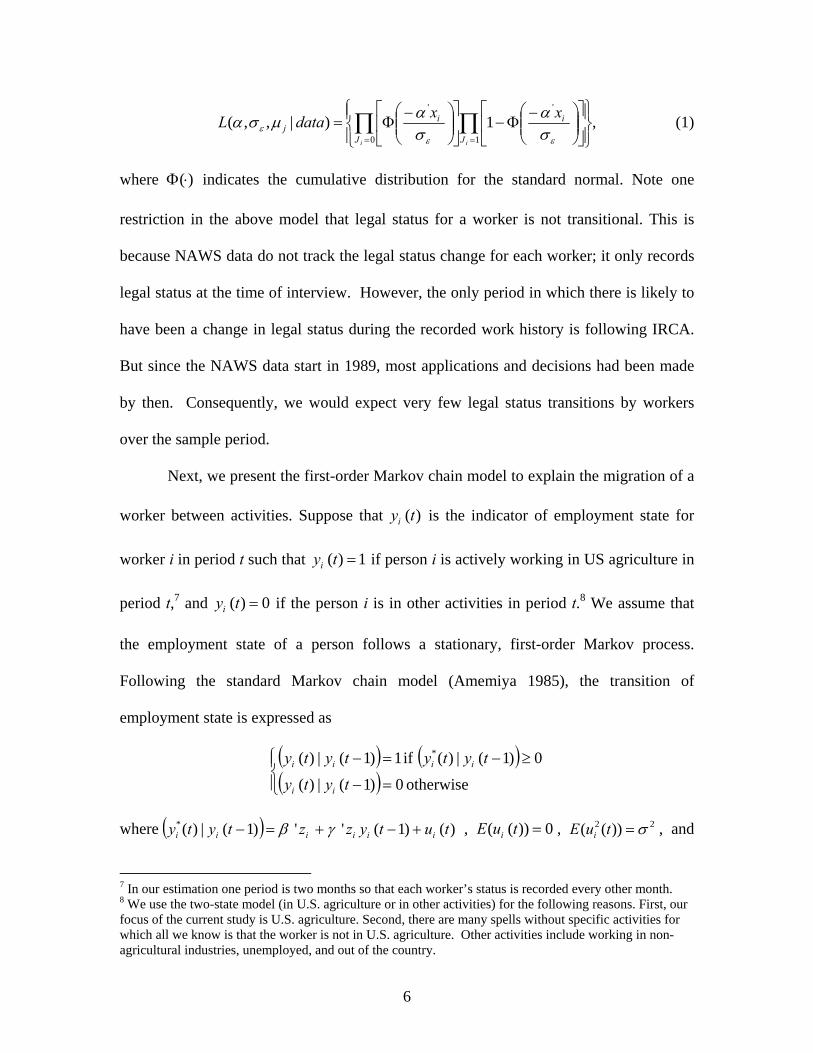
where indicates the cumulative distribution for the standard normal. Note one

restriction in the above model that legal status for a worker is not transitional. This is

because NAWS data do not track the legal status change for each worker; it only records

legal status at the time of interview. However, the only period in which there is likely to

have been a change in legal status during the recorded work history is following IRCA.

But since the NAWS data start in 1989, most applications and decisions had been made

by then. Consequently, we would expect very few legal status transitions by workers

over the sample period.

)(⋅Φ

Next, we present the first-order Markov chain model to explain the migration of a

worker between activities. Suppose that is the indicator of employment state for

worker i in period t such that if person i is actively working in US agriculture in

period t,

)(tyi

1)( =tyi

7 and if the person i is in other activities in period t.0)( =tyi8 We assume that

the employment state of a person follows a stationary, first-order Markov process.

Following the standard Markov chain model (Amemiya 1985), the transition of

employment state is expressed as

( ) ( )( )⎪⎩

⎪⎨⎧

=−

≥−=−

otherwise 0)1(|)(

0)1(|)( if 1)1(|)( *

tyty

tytytyty

ii

iiii

where ( ) )()1('')1(|)(* tutyzztyty iiiiii +−+=− γβ , , , and 0))(( =tuE i22 ))(( σ=tuE i

7 In our estimation one period is two months so that each worker’s status is recorded every other month. 8 We use the two-state model (in U.S. agriculture or in other activities) for the following reasons. First, our focus of the current study is U.S. agriculture. Second, there are many spells without specific activities for which all we know is that the worker is not in U.S. agriculture. Other activities include working in non-agricultural industries, unemployed, and out of the country.

6

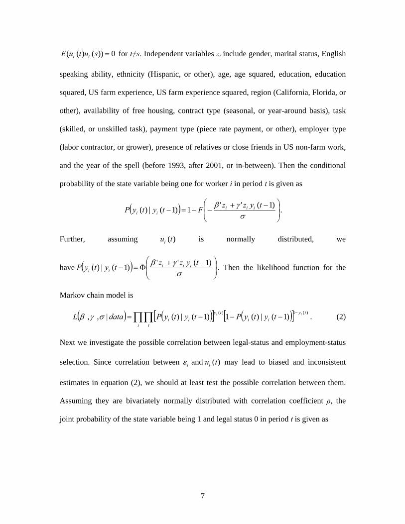
0))()(( =sutuE ii for t≠s. Independent variables zi include gender, marital status, English

speaking ability, ethnicity (Hispanic, or other), age, age squared, education, education

squared, US farm experience, US farm experience squared, region (California, Florida, or

other), availability of free housing, contract type (seasonal, or year-around basis), task

(skilled, or unskilled task), payment type (piece rate payment, or other), employer type

(labor contractor, or grower), presence of relatives or close friends in US non-farm work,

and the year of the spell (before 1993, after 2001, or in-between). Then the conditional

probability of the state variable being one for worker i in period t is given as

( ) ⎟⎟⎠

⎞⎜⎜⎝

⎛ −+−−=−

σγβ )1(''1)1(|)( tyzzFtytyP iii

ii .

Further, assuming is normally distributed, we

have

)(tui

( ) ⎟⎟⎠

⎞⎜⎜⎝

⎛ −+Φ=−

σγβ )1('')1(|)( tyzztytyP iii

ii . Then the likelihood function for the

Markov chain model is

( ) ( )[ ] ( )[ ]∏∏ −−−−=

i t

tyii

tyii

ii tytyPtytyPdataL )(1)( )1(|)(1)1(|)( | ,, σγβ . (2)

Next we investigate the possible correlation between legal-status and employment-status

selection. Since correlation between may lead to biased and inconsistent

estimates in equation (2), we should at least test the possible correlation between them.

Assuming they are bivariately normally distributed with correlation coefficient ρ, the

joint probability of the state variable being 1 and legal status 0 in period t is given as

and ( )i iu tε

7

' xiα−

( ) ( ) )(),(,)1(|0,1)()1(

2''

tdudtutyjtyP iityzz

iiii

iii

ερεφ

σ

γβ

σ ε

∫ ∫∞

−+−

∞−

=−== .

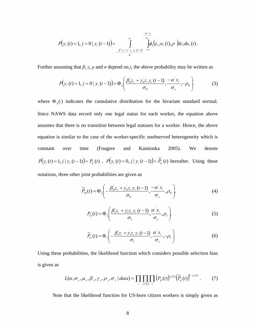
Further assuming that β, γ, ρ and σ depend on j, the above probability may be written as

( ) .,,)1()1(|0,1)('

0

'0

'0 ⎟

⎠

⎞⎜⎝

⎛−

−−+Φ=−== ρ

σα

σγβ

ε

iiii xtyzztyjtyP (3)

where )(2 ⋅Φ indicates the cumulative distribution for the bivariate standard normal.

Since NAWS data record only one legal status for each worker, the equation above

on orker. Hence, the above

equation is similar to the case of the worker-specific unobser

02 ⎟⎜ii

assum there is no transiti between legal statuses for a w

ved heterogeneity which is

constant over time (Fougere and Kamionka 2005). We denote

es that

( ) )()1(|,1)( tPtyjtyP ijii =−= , ( ) )(~)1(|,0)( tPtyjtyP ijii =−= hereafter. Using these

notations, three other joint probabilities are given as

,,,)1()(~0

'

0

'0

'0

20 ⎟⎟⎠

⎞⎜⎜⎝

⎛ −−+−Φ= ρ

σα

σγβ

ε

iiiii

xtyzztP (4)

,,,)1()( 1

'

121 ⎟

⎠⎜⎝ σσ ε

i

'1

'1 ⎟

⎞⎜⎛ −+

Φ= ραγβ iiii xtyzztP (5)

.,,)1()(~1

'

1

'1

'1

21 ⎟⎟⎠

⎞⎜⎜⎝

⎛−

−+−Φ= ρ

σα

σγβ

ε

iiiii

xtyzztP (6)

Using these probabilities, the likelihood function which considers possible selection bias

is given

as

( ) ( ) −=i

ty

j tij

tyijjjjjj

i )(1

1,0

)( ~

Note that the likelihood function for US-born citizen workers is simply given as

∏∏∏= i tPtPdataL )()() | ,,,,,,( σργβµσα ε . (7)

8

equation (2) since they do not have the legal-status-selection problem. Next, we introduce

tests for existence of sample selection bias in the above estimation. That is, we test

whether the ρj’s are significantly different from zero. The simplest test is checking t-

statistics for each ρj. The problem with this method is that there are many inconclusive

cases since it is possible to have a different test result for each ρj. More systematic test

methods are the likelihood ratio (LR) test and Wald test. It can be shown that maximizing

equation (7) is the identical problem as maximizing equation (1) for legal status 0 and 1,

and equation (2) separately for each legal status, if there is no sample selection bias (ρj=0

for j=0 and 1). Then the large sample distribution of -2*lnλ, where λ is the likelihood

ratio of restricted over unrestricted maximum likelihood, follows a chi-square distribution

ith degrees of freedom of 2. While the LR test requires both unrestricted and restricted

maximum likelihood estimators, the Wal ator.

These t

w

d test requires only the unrestricted estim

ests are standard, and we follow the formulas in Greene (2003).

Data

The data used in this study are obtained from the National Agricultural Workers Survey

(NAWS) (U.S. Department of Labor 2006). The survey reports each worker’s work-history for

three years at maximum preceding the date of interview. We used the study period from 1989,

when the NAWS was first available, to the most recent year available, 2004, with sample size of

40,650

workers.9 We record the employment status (in US agriculture or in other activities) of

each worker every other month for three years at maximum. Next we describe the definitions of

each variable used in the model below.

Legal status is a discrete variable ranging from 0 to 2. A foreign born worker must fall

9 This sample size is much larger than 1,538 in Tran and Perloff (2002).

9

into status 0 or 1. Status 0 = “unauthorized” worker means that the worker is undocumented (did

not apply to any legal status or application was denied) and also includes one who had no work

authorization even if he is documented. Status 1 = “authorized” worker includes naturalized

citizen,

). Skilled Task is a dummy for

workers

employer. It does not include those

who ow

green card holder and work authorization holder; the work authorization may fall into any

of the following: border crossing card/commuter card, pending status, or temporary resident

status with a non-immigrant visa. The US-born citizen has status 2 = “citizen” by birth.

The variable English measures the capability to speak English. The variable is a discrete

variable ranging from 1 to 4, where 1 = not speaking English at all, 2 = speak a little English, 3 =

somewhat able to speak English, and 4 = speaking English well. Hispanic is a dummy variable

for Hispanic which includes Mexican-American, Mexican, Chicano, Puerto Rican, and other

Hispanic ethnic groups. Black (or African American) and White are also dummy variables derived

from a question regarding their race which may also be American Indian/Alaka Native,

Indigenous, Asian, Native Hawaiian or Pacific Islander, or others. Age was calculated from the

difference between the beginning date of spell and the date of birth. Education is the highest

grade level for education, and it ranges from 0 to 20. Experience is the number of years of doing

farm work in the US (not including farm work experience abroad

who engage in semi-skilled or supervisory tasks. Although the original questions have

over 100 task codes, tasks are grouped into six categories as follows: 1 = pre-harvest, 2 = harvest,

3 = post-harvest, 4 = semi-skilled, 5 = supervisor, and 6 = other.

Seasonal Worker is a dummy for workers who were working on a seasonal basis for the

employer. Piece rate is a dummy for workers who are paid by piece rate instead of being paid by

the hour or a salary. Labor contractor is a dummy variable for workers who are employed by

labor contractors rather than the grower. Free housing is a dummy variable for workers (or

workers and their family) who receive free housing from their

n their house or live for free with friends or relatives. It also excludes those who pay for

housing provided by employers or by the government or charity. Relative is a dummy for workers

10

who have relatives or close friends in US non-farm work.

The dummies for Florida and California are the location of the employment. Before 1993

dummy variable is for all the years p majority of IRCA legalization was

granted

rior to 1993 when the

, and After 2001 is the years post-September 11, 2001 event.

Empirical Results

For legal status 0 and 1 workers, we estimated the Markov chain model with self-

selectivity using the Newton-Raphson method with the maximum likelihood function

iven as equation (7).10 Since status 2 workers (citizens by birth), do not have the legal-

, we simply estimated equation (2) for this group using the same

method

Using a 0.05 significance cr

find that all coefficients are statistically significant. The third column of Table 1 shows

the marginal effect of each variable on the probability of a worker being legal. The

probability of worker i being legal is given by

g

status-selection problem

.

Legal status selection

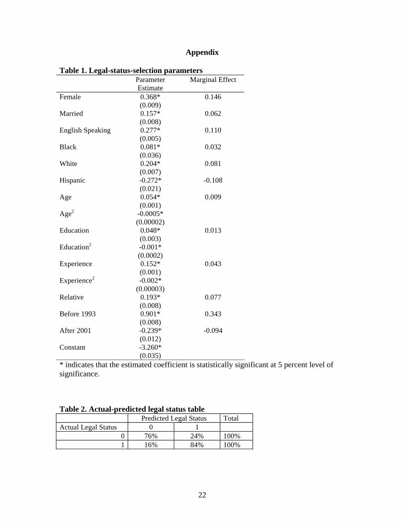
The estimates for legal-status-selection parameters in equation (7) and their

asymptotic standard errors are reported in table 1. iterion, we

*Pr ob( 0) 1 ( ' )i iJ x α> = −Φ − . Then the

marginal effect of variable k evaluated at the mean x is kx ααφ )'(− for the continuous

variables and )'()'( kkkkk xx ααα −−Φ−−Φ les, where −−−− for the dummy variab k−

k−

x ' and

α are variables and coefficients excluding the k . Females, married, workers with

higher English speaking ability, black, white, non-hispanic, with a relative in the US non-

th

10 We calculated gradient vector and Hessian matrix for logarithm of equation (7).

11

agricultural sector are statistically significantly more likely to have legal status all else

being the same. We also find that age, education and US farm experience have a

significant nonlinear effect on legal status. All three are positive almost throughout the

relevant range: US farm experience has a positive effect on legal status up to 34 years;

education has a positive effect on legal status up to 18 years, and age has a positive effect

on legal status up to 55 years. We find that the greatest positive marginal effect is from

the Before 1993 dummy followed by Female dummy and English speaking ability. The

greatest negative marginal effect is from the Hispanic dummy followed by the After 2001

dummy

ose emp

atus table. A worker is

predicted to be status 0 (unauthorized) if

. Note that, holding all other characteristics the same, the workers employed

before 1993 are 34% more likely and those interviewed after 2001 are 9% less likely to

be legal compared to th loyed between these periods.

Finally, Table 2 shows the actual-predicted legal st

0'ˆ <ixα , and is predicted to be status 1

(authorized) worker if 0'ˆ >ixα . Table 2 shows that 76% of unauthorized, and 84% of

authori

rentheses)

the coefficients on the selectivity variables

zed workers are correctly predicted in their legal status.

Employment state transition

The estimates for employment-state-transition parameters in equation (7) and

their asymptotic standard errors (given in the pa are reported in tables 3 and 4.

Status 0 (unauthorized) workers have 85,556 spells; status 1 (authorized) workers have

101,132 spells. Based on asymptotic standard errors using a 0.05 significance criterion,

0ρ and 1ρ are both highly significantly

12

negative.11 We have the same conclusion using LR test and Wald test. We have the

computed log likelihood ratio of 16.642 and Wald statistics of 34.443 both of which are

larger than the critical value of 5.991 with 2 degree of freedom at 5 % level of

significance. That is, using maximum likelihood estimator for equation (2) for each legal

status

alifornia, Florida, Skilled task worker (in agriculture) and After 2001

without correcting for self-selectivity would lead to bias in estimates for both

unauthorized and authorized workers.

Table 3 presents the employment transition parameters and asymptotic standard

errors for legal status 0 (unauthorized) and legal status 1 (authorized) worker given

previous state is “not in US agriculture”. This corresponds to estimate of 0β in equation

(3) and (4) for status 0 and 1β in equation (5) and (6) for status 1 worker. A positive

estimate means that it has a positive effect on the probability of being in US agriculture

given the previous state is not in US agriculture. We find that most of the estimates are

statistically significant and have the same sign for both legal statuses, except for a few

variables such as seasonal worker dummy and Before 1993 dummy. The former has

negative effect for authorized worker, but no significant effect for unauthorized worker,

while Before 1993 dummy has negative effect for unauthorized worker but no significant

effect for authorized worker. Females, married, workers with higher English speaking

ability, with free-housing, employed by labor contractors are statistically significantly

less likely to be into agriculture from other employment state, all else being the same. On

the other hand, C

11 The negative correlation between iε and does not mean that selection bias has negative effect on probability of being in US agriculture. This is especially true for the case of legal status 0 worker for whom being in US agriculture means that and .

)(tui

0'0

'0 /))1(()( σγβ −+−> tyzztu iiii εσαε /'

ii x−<

13

dummy

argest for the Hispanic dummy

followe

asympto

errors for each legal status worker given the previous state is “in US agriculture”. This is

calculated from in equations (3) and (4) for status 0 and in equations

have significantly positive effect on probability of being into agriculture, all else

being the same.

The third and fifth columns in table 3 show the marginal effects of each variable

on the joint probability of being in the respective legal status and in US agriculture. This

joint probability is given as equation (3) for unauthorized worker and equation (5) for

authorized worker. Marginal effects are evaluated at the mean of independent variables

for each legal status worker. Note that the marginal effects of some variables have

opposite signs to the partial effect on being in US agriculture, which is given as the

estimated coefficient. These variables are Marital status, Relative dummy and English

speaking ability for authorized workers, and Hispanic dummy for unauthorized workers.

All these variables have a very strong effect on being in the respective legal status,

especially the Marital status dummy and English speaking ability on being authorized,

and the Hispanic dummy on being an unauthorized worker. Although these variables

have a negative effect on being in US agriculture, the positive effect on the legal status

must dominate. As for the magnitude of the marginal effect for unauthorized workers, the

negative effect is largest for Before 1993 dummy followed by the Marital status dummy,

while the positive effect is largest for the California dummy followed by the After 2001

dummy. For authorized workers, the negative effect is l

d by the Labor contractor dummy, while the positive effect is largest for the

Before 1993 dummy followed by the California dummy.

Table 4 shows the employment transition parameters and tic standard

)ˆˆ( 00 γβ + )ˆˆ( 11 γβ +

14

(5) and (6) for status 1 workers.12 A positive estimate means that it has a positive effect

on the probability of being in US agriculture given the previous state is in US agriculture.

We find that most of the estimates are statistically significant and have the same sign for

both legal statuses, except for a few variables. For example, English speaking ability has

no significant effect for either legal status worker, while Marital status dummy has a

negative effect for unauthorized, and the Hispanic dummy has a positive effect for

authorized workers, but no significant effect on the other. Both Labor contractor and the

Piece rate payment dummies have negative effects for authorized workers, but no

significant effect for unauthorized workers.

Other than these variables, females, seasonal workers with a relative in US non-

agriculture sector, with free-housing, in California, before 1993 are statistically

significantly less likely to stay in US agriculture, all else being the same. Note also that

education has a negative effect on staying in US agriculture at the mean for both legal

statuses.13 On the other hand, Florida, After 2001, and Skilled task worker (in agriculture)

dummies have significantly positive effects, all else being the same.

The third and fifth columns in table 4 show the marginal effects of each variable

on the joint probability of being in the respective legal status and remaining in US

agriculture. This joint probability is given as equation (3) for the unauthorized worker

and equation (5) for the authorized worker. Again, marginal effects of some variables

have opposite signs to the partial effect on being in US agriculture, given as the estimated

coefficient. This happens only for authorized workers. These variables are Female,

12 We also used the following formula to calculate estimate for variance and standard errors:

Est. . )γ,β(*Est.)γ(Est.)β(Est.)γβ( jjjjjj ˆˆcov2ˆvarˆvarˆˆvar ++=+

15

Marital status, Relative and Before 1993 dummy and Education, all of which have very

strong positive effects on being in an authorized legal status. Although these variables

have negative effects on staying in US agriculture, the positive effects on the legal status

must dominate. Also, strong negative effects on legal status of Hispanic and After 2001

dummies dominate the positive effect on staying in US agriculture.

As for the magnitude of the marginal effect for unauthorized workers, the

negative effect is largest from the Before1993 dummy followed by the Female dummy,

while the positive effect is largest from the Hispanic dummy followed by the Florida

dummy. For authorized workers, the negative effect is largest from the Seasonal worker

dummy followed by the Hispanic dummy, while the positive effect is largest from the

Before1993 dummy followed by the Florida dummy. Before 1993, it is almost 30% less

likely to remain in US agriculture with an unauthorized worker status, and 23% more

likely to remain in US agriculture with an authorized worker status, all else being the

same.

Finally table 5 shows the estimates and their asymptotic standard errors for the

Markov chain model for US-born citizen workers. Here we estimated equation (2) using

the maximum likelihood method. We also calculated the marginal effect on the

probability of being in US agriculture at the mean of independent variables. We find the

strongest negative effect on moving into agriculture is from the Labor contractor and

Before 1993 dummies, and the strongest positive effect is from the After 2001 dummy

followed by the California dummy. The strongest negative effect on staying in US

agriculture is from the Seasonal worker dummy followed by Free housing and Relative

13 Education has negative effect up to 8.6 years for unauthorized workers and 6.5 years for authorized

16

dummy, and the strongest positive effect is from the Florida dummy followed by the

Skilled task worker (in agriculture) dummy.

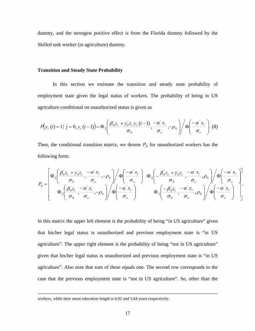
Transition and Steady State Probability

In this section we estimate the transition and steady state probability of

employment state given the legal status of workers. The probability of being in US

agriculture conditional on unauthorized status is given as

( ) ⎟⎟⎠

⎞⎜⎜⎝

⎛ −Φ⎟

⎟⎠

⎞⎜⎜⎝

⎛−

−−+Φ=−==

εε σα

ρσα

σγβ iiiii

ii

xxtyzztyjtyP

'

0

'

0

'0

'0

2 ,,)1(

)1(,0|1)( . (8)

Then, the conditional transition matrix, we denote Pj, for unauthorized workers has the

following form:

.,,,,

,,,,

'

0

'

0

'0

2

'

0

'

0

'0

2

'

0

'

0

'0

'0

2

'

0

'

0

'0

'0

2

0

⎥⎥⎥⎥⎥

⎦

⎤

⎢⎢⎢⎢⎢

⎣

⎡

⎟⎟⎠

⎞⎜⎜⎝

⎛ −Φ⎟

⎟⎠

⎞⎜⎜⎝

⎛ −−Φ⎟

⎟⎠

⎞⎜⎜⎝

⎛ −Φ⎟

⎟⎠

⎞⎜⎜⎝

⎛−

−Φ

⎟⎟⎠

⎞⎜⎜⎝

⎛ −Φ⎟

⎟⎠

⎞⎜⎜⎝

⎛ −+−Φ⎟

⎟⎠

⎞⎜⎜⎝

⎛ −Φ⎟

⎟⎠

⎞⎜⎜⎝

⎛−

−+Φ

=

εεεε

εεεε

σα

ρσα

σβ

σα

ρσα

σβ

σα

ρσα

σγβ

σα

ρσα

σγβ

iiiiii

iiiiiiii

xxzxxz

xxzzxxzz

P

In this matrix the upper left element is the probability of being “in US agriculture” given

that his/her legal status is unauthorized and previous employment state is “in US

agriculture”. The upper right element is the probability of being “not in US agriculture”

given that his/her legal status is unauthorized and previous employment state is “in US

agriculture”. Also note that sum of these equals one. The second row corresponds to the

case that the previous employment state is “not in US agriculture”. So, other than the

workers, while their mean education length is 6.02 and 5.64 years respectively.

17

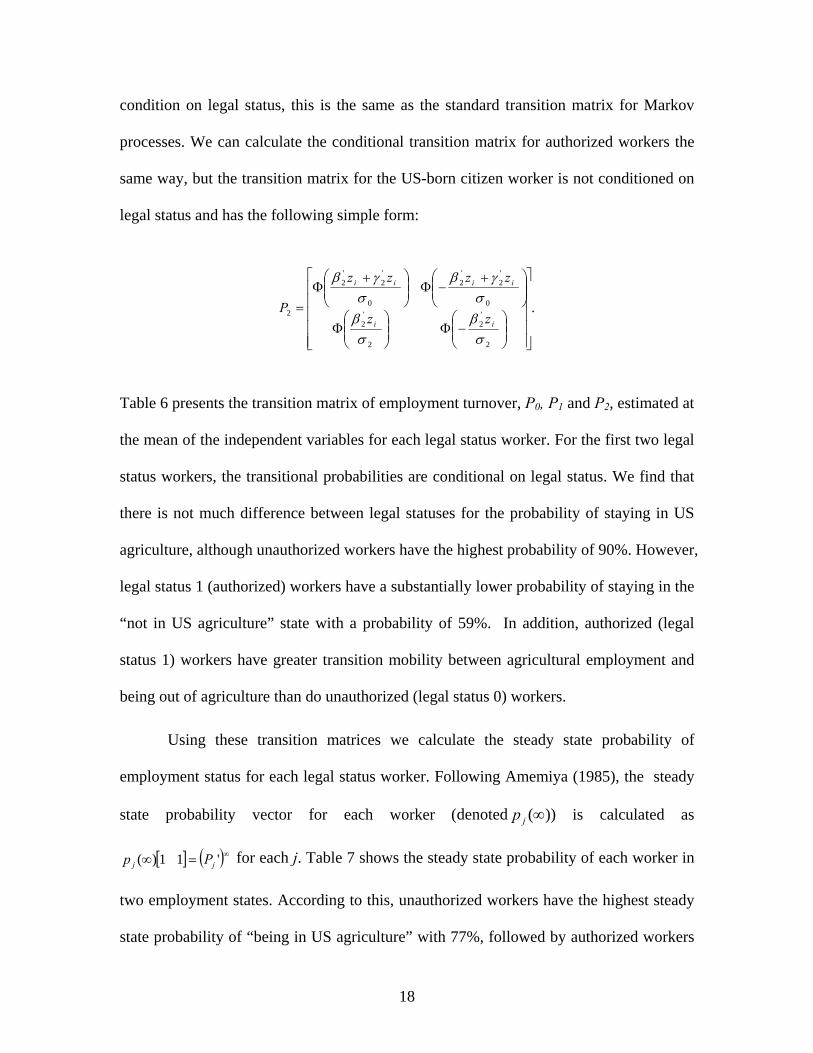
condition on legal status, this is the same as the standard transition matrix for Markov

processes. We can calculate the conditional transition matrix for authorized workers the

same way, but the transition matrix for the US-born citizen worker is not conditioned on

legal status and has the following simple form:

.

2

'2

2

'2

0

'2

'2

0

'2

'2

2

⎥⎥⎥⎥⎥

⎦

⎤

⎢⎢⎢⎢⎢

⎣

⎡

⎟⎟⎠

⎞⎜⎜⎝

⎛−Φ⎟⎟

⎠

⎞⎜⎜⎝

⎛Φ

⎟⎟⎠

⎞⎜⎜⎝

⎛ +−Φ⎟⎟

⎠

⎞⎜⎜⎝

⎛ +Φ

=

σβ

σβ

σγβ

σγβ

ii

iiii

zz

zzzz

P

Table 6 presents the transition matrix of employment turnover, P0, P1 and P2, estimated at

the mean of the independent variables for each legal status worker. For the first two legal

status workers, the transitional probabilities are conditional on legal status. We find that

there is not much difference between legal statuses for the probability of staying in US

agriculture, although unauthorized workers have the highest probability of 90%. However,

legal status 1 (authorized) workers have a substantially lower probability of staying in the

“not in US agriculture” state with a probability of 59%. In addition, authorized (legal

status 1) workers have greater transition mobility between agricultural employment and

being out of agriculture than do unauthorized (legal status 0) workers.

Using these transition matrices we calculate the steady state probability of

employment status for each legal status worker. Following Amemiya (1985), the steady

state probability vector for each worker ))( denoted( ∞jp is calculated as

for each j. Table 7 shows the steady state probability of each worker in

two employment states. According to this, unauthorized workers have the highest steady

state probability of “being in US agriculture” with 77%, followed by authorized workers

[ ] ( )∞=∞ '11)( jj Pp

18

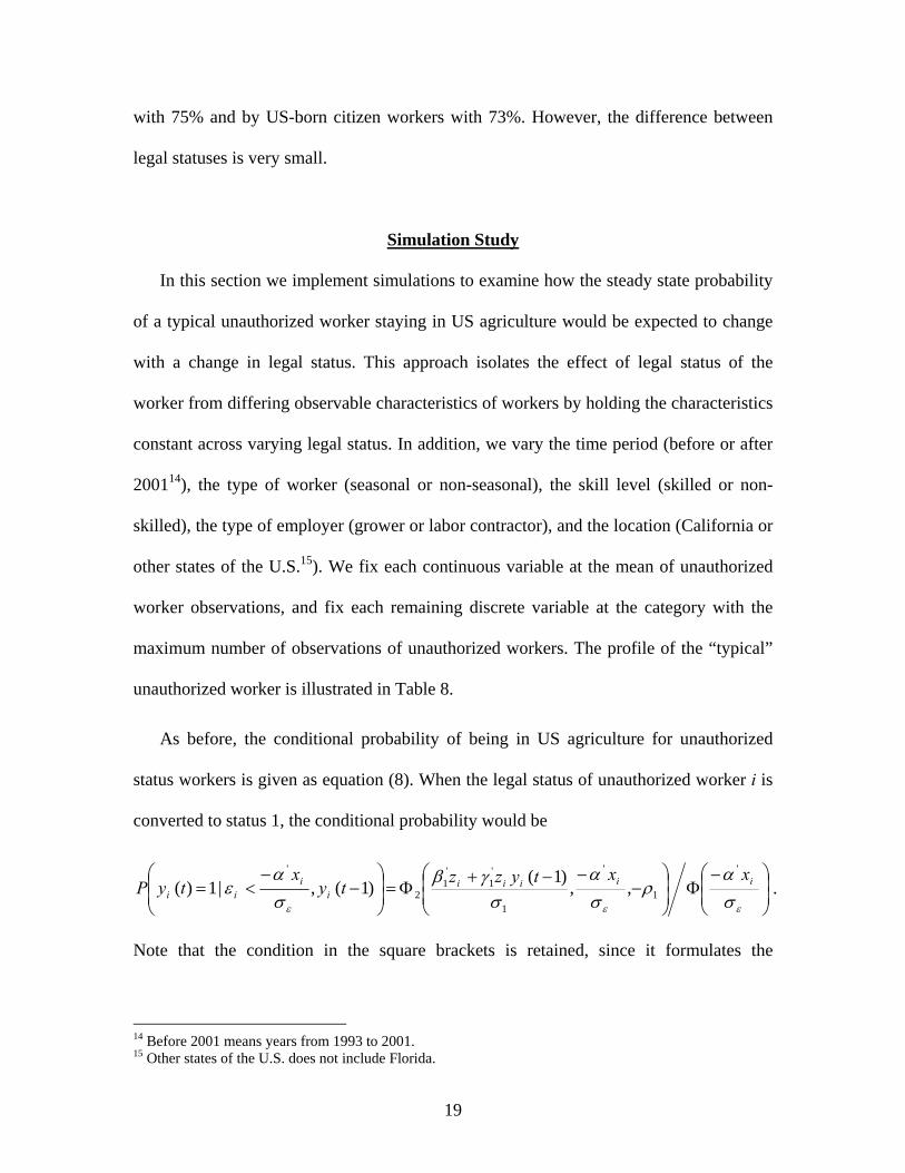
with 75% and by US-born citizen workers with 73%. However, the difference between

legal statuses is very small.

Simulation Study

In this section we implement simulations to examine how the steady state probability

of a typical unauthorized worker staying in US agriculture would be expected to change

with a change in legal status. This approach isolates the effect of legal status of the

worker from differing observable characteristics of workers by holding the characteristics

constant across varying legal status. In addition, we vary the time period (before or after

200114), the type of worker (seasonal or non-seasonal), the skill level (skilled or non-

skilled), the type of employer (grower or labor contractor), and the location (California or

other states of the U.S.15). We fix each continuous variable at the mean of unauthorized

worker observations, and fix each remaining discrete variable at the category with the

maximum number of observations of unauthorized workers. The profile of the “typical”

unauthorized worker is illustrated in Table 8.

As before, the conditional probability of being in US agriculture for unauthorized

status workers is given as equation (8). When the legal status of unauthorized worker i is

converted to status 1, the conditional probability would be

⎟⎟⎠

⎞⎜⎜⎝

⎛ −Φ⎟

⎟⎠

⎞⎜⎜⎝

⎛−

−−+Φ=⎟

⎟⎠

⎞⎜⎜⎝

⎛−

−<=

εεε σα

ρσα

σγβ

σα

ε iiiiii

iii

xxtyzztyx

tyP'

1

'

1

'1

'1

2

'

,,)1()1(,|1)( .

Note that the condition in the square brackets is retained, since it formulates the

14 Before 2001 means years from 1993 to 2001. 15 Other states of the U.S. does not include Florida.

19

unobservable characteristics for legal status selection of the worker i.16 In the same way

we calculate the conditional probabilities for the other three elements in the transition

matrix, then calculate the steady state probability in US agriculture. Finally, we calculate

the change in the steady state probability from this legal status conversion.

The results are shown in Table 9. For 27 out of 32 cases, unauthorized workers

working as “legal” workers would have a higher steady state probability in US

agriculture than when working as unauthorized workers. If we focus on before 1993 cases,

in all 16 cases, legal status would increase the steady state probability in US agriculture,

but the magnitude of the change is not large. The highest increase is for seasonal,

unskilled workers employed by growers not in California with a 7.3% point increase.

There are only four cases with changes greater than 5% points, all of which occur for

workers employed by growers. These five cases tend to be unskilled (with one exception)

and seasonal workers (with one exception).

There are five cases after 2001 in which legal status would decrease the steady

state probability in US agriculture. Interestingly, all of these cases are for workers

employed by labor contractors. However, the largest decrease is only 1.1% point for

seasonal, skilled workers employed by labor contractors in California. Overall, we could

say that the change in the steady state probability from legal status conversion is very

small after 2001; none of the 16 cases is over 5% points in absolute value.

Conclusion

We have proposed and estimated a stationary, first-order Markov chain model

with selection bias correction to adequately estimate the likelihood of each legal status

16 See Maddala (1983) for the detailed argument.

20

worker staying in U.S. agriculture. We used the NAWS data from 1989, when the NAWS

was first available, to the most recent year available, 2004, with a sample size of 40,650

workers, and recorded the employment status (in US agriculture or in other activities) of

each worker every other month for three years at maximum.

Our maximum likelihood estimation shows statistically significant coefficients on

the selection bias terms for both authorized and unauthorized workers. Then we corrected

selection bias in the calculation of transition and steady state probabilities of employment

turnover. The conditional steady state probability in US agriculture is highest for

unauthorized workers, but there is not much difference between legal statuses. Also, the

simulation study shows that a legal status change for unauthorized worker would result in

only small changes in the steady state probability of being in US agriculture, especially

after 2001. The dramatic increase in composition of unauthorized workers in US

agriculture during 1990s remains unexplained since our results find too small a difference

in employment turnover between legal statuses to explain that phenomenon. The next

issue is to study the entry into and exit out of US agriculture: what type of worker entered

and left US agriculture.

21

Appendix

Table 1. Legal-status-selection parameters

* indicates that the estimated coefficient is statistically significant at 5 percent level of significance.

Parameter Estimate

Marginal Effect

Female 0.368* (0.009)

0.146

Married 0.157* (0.008)

0.062

English Speaking 0.277* (0.005)

0.110

Black 0.081* (0.036)

0.032

White 0.204* (0.007)

0.081

Hispanic -0.272* (0.021)

-0.108

Age 0.054* (0.001)

0.009

Age2 -0.0005* (0.00002)

Education 0.048* (0.003)

0.013

Education2 -0.001* (0.0002)

Experience 0.152* (0.001)

0.043

Experience2 -0.002* (0.00003)

Relative 0.193* (0.008)

0.077

Before 1993 0.901* (0.008)

0.343

After 2001 -0.239* (0.012)

-0.094

Constant -3.260* (0.035)

Table 2. Actual-predicted legal status table Predicted Legal Status Total Actual Legal Status 0 1

0 76% 24% 100% 1 16% 84% 100%

22

Table 3. Employment transition parameters when the previous state is “not in US agriculture”. Unauthorized Marginal

Effect Authorized Marginal

Effect Female -0.123*

(0.021) -0.060 -0.197*

(0.018) -0.004

Married -0.281* (0.017)

-0.092 -0.055* (0.018)

0.007

English Speaking -0.040* (0.013)

-0.030 -0.027* (0.010)

0.032

Hispanic -0.060 (0.059)

0.001 -0.166* (0.037)

-0.088

Age 0.079* (0.003)

0.004 0.029* (0.004)

0.003

Age2 -0.001* (0.00004)

-0.0003* (0.00004)

Education 0.024* (0.008)

-0.002 0.013 (0.007)

0.004

Education2 -0.002* (0.001)

-0.001* (0.0005)

Experience -0.010* (0.004)

-0.011 0.018* (0.004)

0.015

Experience2 0.0002* (0.00007)

-0.0003* (0.00008)

California 0.298* (0.019)

0.086 0.274* (0.017)

0.080

Florida 0.081* (0.026)

0.024 0.250* (0.030)

0.073

Free Housing -0.050* (0.020)

-0.014 -0.058* (0.020)

-0.017

Seasonal Worker 0.020 (0.017)

0.006 -0.131* (0.015)

-0.039

Skilled Task 0.109* (0.024)

0.032 0.132* (0.019)

0.039

Piece Rate 0.010 (0.019)

0.003 0.040* (0.017)

0.012

Labor Contractor -0.074* (0.019)

-0.022 -0.154* (0.018)

-0.045

Relative -0.064* (0.018)

-0.031 -0.022 (0.016)

0.022

Before 1993 -0.183* (0.025)

-0.112 0.043 (0.022)

0.143

After 2001 0.228* (0.026)

0.082 0.150* (0.031)

0.010

Constant -1.685* (0.085)

-0.759* (0.123)

Rho -0.199* (0.039)

-0.110* (0.038)


23

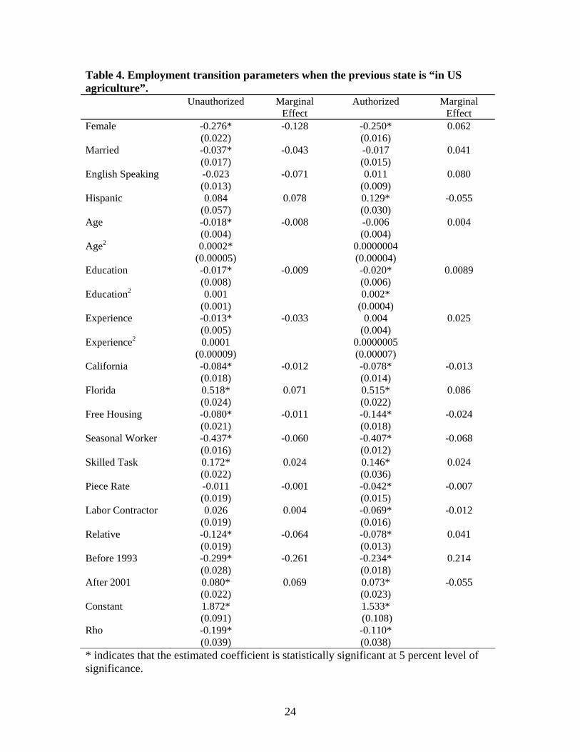
Table 4. Employment transition parameters when the previous state is “in US agriculture”. Unauthorized Marginal

Effect Authorized Marginal


(0.022) -0.128 -0.250*

(0.016) 0.062

Married -0.037* (0.017)

-0.043 -0.017 (0.015)

0.041

English Speaking -0.023 (0.013)

-0.071 0.011 (0.009)

0.080

Hispanic 0.084 (0.057)

0.078 0.129* (0.030)

-0.055

Age -0.018* (0.004)

-0.008 -0.006 (0.004)

0.004

Age2 0.0002* (0.00005)

0.0000004 (0.00004)

Education -0.017* (0.008)

-0.009 -0.020* (0.006)

0.0089

Education2 0.001 (0.001)

0.002* (0.0004)

Experience -0.013* (0.005)

-0.033 0.004 (0.004)

0.025

Experience2 0.0001 (0.00009)

0.0000005 (0.00007)

California -0.084* (0.018)

-0.012 -0.078* (0.014)

-0.013

Florida 0.518* (0.024)

0.071 0.515* (0.022)

0.086

Free Housing -0.080* (0.021)

-0.011 -0.144* (0.018)

-0.024

Seasonal Worker -0.437* (0.016)

-0.060 -0.407* (0.012)

-0.068


0.024 0.146* (0.036)

0.024

Piece Rate -0.011 (0.019)

-0.001 -0.042* (0.015)

-0.007

Labor Contractor 0.026 (0.019)

0.004 -0.069* (0.016)

-0.012

Relative -0.124* (0.019)

-0.064 -0.078* (0.013)

0.041

Before 1993 -0.299* (0.028)

-0.261 -0.234* (0.018)

0.214

After 2001 0.080* (0.022)

0.069 0.073* (0.023)

-0.055

Constant 1.872* (0.091)

1.533* (0.108)

Rho -0.199* (0.039)

-0.110* (0.038)


24

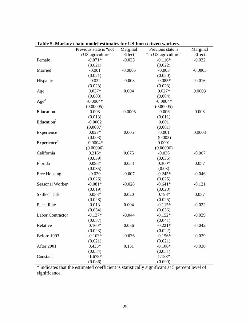
Table 5. Markov chain model estimates for US-born citizen workers. Previous state is “not

in US agriculture” Marginal

Effect Previous state is

“in US agriculture” Marginal


(0.021) -0.025 -0.116*

(0.022) -0.022

Married -0.001 (0.021)

-0.0005 -0.003 (0.020)

-0.0005

Hispanic -0.022 (0.023)

-0.008 -0.085* (0.023)

-0.016

Age 0.037* (0.003)

0.004 0.027* (0.004)

0.0003

Age2 -0.0004* (0.00005)

-0.0004* (0.00005)

Education 0.003 (0.013)

-0.0005 -0.006 (0.011)

0.003

Education2 -0.0002 (0.0007)

0.001 (0.001)

Experience 0.027* (0.003)

0.005 -0.001 (0.003)

0.0003

Experience2 -0.0004* (0.00006)

0.0001 (0.00006)

California 0.216* (0.039)

0.075 -0.036 (0.035)

-0.007

Florida 0.093* (0.035)

0.033 0.300* (0.03)

0.057

Free Housing -0.020 (0.026)

-0.007 -0.245* (0.025)

-0.046

Seasonal Worker -0.081* (0.019)

-0.028 -0.641* (0.020)

-0.121


0.020 0.198* (0.025)

0.037

Piece Rate 0.013 (0.034)

0.004 -0.115* (0.036)

-0.022

Labor Contractor -0.127* (0.037)

-0.044 -0.152* (0.041)

-0.029

Relative 0.160* (0.023)

0.056 -0.221* (0.022)

-0.042

Before 1993 -0.103* (0.021)

-0.036 -0.156* (0.021)

-0.029

After 2001 0.433* (0.034)

0.151 -0.106* (0.031)

-0.020

Constant -1.678* (0.086)

1.183* (0.090)


25

Table 6. Transition matrix for each legal status worker. Employments state=1 Employments state=0

Legal status 0 Previous employment state=1 0.904 0.096 Previous employment state=0 0.321 0.679



Employment state 1 is “in US agriculture” and Employment state 0 is “not in US agriculture”. One period is two months. Status 0 and status 1 worker probabilities are conditional on legal status. Table 7. Steady state probability of employment state. Legal status 0

Employment state=1 0.770 Employment state=0 0.230

Legal status 1 Employment state=1 0.746 Employment state=0 0.254

Legal status 2 Employment state=1 0.733 Employment state=0 0.267

Table 8. Profile of the “Typical” Unauthorized Worker Female 0 Married 0 English Speaking 1.506 Black 0 White 0 Hispanic 1 Age 27.880 Education 6.020 Experience 5.436 Florida 0 Free Housing 0 Piece Rate 0 Before 1993 0 Relative 0 Constant 1

26

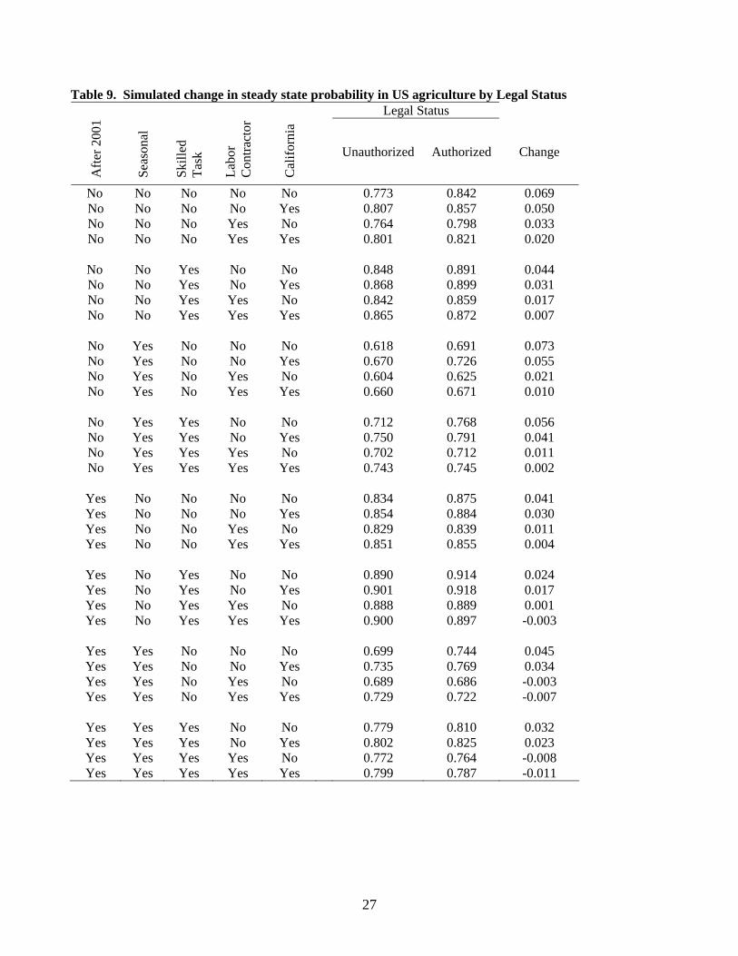
Table 9. Simulated change in steady state probability in US agriculture by Legal StatusLegal Status

Afte

r 200

1

Seas

onal

Skill

ed

Task

Labo

r C

ontra

ctor

Cal

iforn

ia

Unauthorized Authorized Change

No No No No No 0.773 0.842 0.069 No No No No Yes 0.807 0.857 0.050 No No No Yes No 0.764 0.798 0.033 No No No Yes Yes 0.801 0.821 0.020

No No Yes No No 0.848 0.891 0.044 No No Yes No Yes 0.868 0.899 0.031 No No Yes Yes No 0.842 0.859 0.017 No No Yes Yes Yes 0.865 0.872 0.007

No Yes No No No 0.618 0.691 0.073 No Yes No No Yes 0.670 0.726 0.055 No Yes No Yes No 0.604 0.625 0.021 No Yes No Yes Yes 0.660 0.671 0.010

No Yes Yes No No 0.712 0.768 0.056 No Yes Yes No Yes 0.750 0.791 0.041 No Yes Yes Yes No 0.702 0.712 0.011 No Yes Yes Yes Yes 0.743 0.745 0.002

Yes No No No No 0.834 0.875 0.041 Yes No No No Yes 0.854 0.884 0.030 Yes No No Yes No 0.829 0.839 0.011 Yes No No Yes Yes 0.851 0.855 0.004

Yes No Yes No No 0.890 0.914 0.024 Yes No Yes No Yes 0.901 0.918 0.017 Yes No Yes Yes No 0.888 0.889 0.001 Yes No Yes Yes Yes 0.900 0.897 -0.003

Yes Yes No No No 0.699 0.744 0.045 Yes Yes No No Yes 0.735 0.769 0.034 Yes Yes No Yes No 0.689 0.686 -0.003 Yes Yes No Yes Yes 0.729 0.722 -0.007

Yes Yes Yes No No 0.779 0.810 0.032 Yes Yes Yes No Yes 0.802 0.825 0.023 Yes Yes Yes Yes No 0.772 0.764 -0.008 Yes Yes Yes Yes Yes 0.799 0.787 -0.011

27

References

Amemiya, T. 1985. Advanced Econometrics. Cambridge, MA: Harvard University

Press.

Carroll, D., R. Samardick, S. Bernard, S. Gabbard, T. Hernandez. 2005. “Findings from

the National Agricultural Workers Survey (NAWS) 2001 - 2002. A Demographic

and Employment Profile of United States Farm Workers.” Research Rpt. No. 9,

Office of Programmatic Policy, Office of Asst. Secretary for Policy. U.S. Dept.

of Labor. (March).

Emerson, R. D. 1989. “Migratory Labor and Agriculture.” American Journal of

Agricultural Economics. 71:617-29.

Emerson, R. D., and O. Napasintuwong. 2002. “Foreign Workers in Southern

Agriculture.” Selected paper, Southern Agricultural Economics Association

Annual Meeting, Orlando, Florida (February).

Fougere, D. and T. Kamionka. 2005. "Econometrics of Individual Labor Market

Transitions." IZA Discussion Paper No. 1850, Institute for the Study of Labor,

Bonn, Germany. (November).

Greene, W. H. 2003. Econometric Analysis, 5th Edition. Upper Saddle River, N.J.:

Prentice Hall.

Hashida, E., and J. M. Perloff. 1996. “Duration of Agricultural Employment.” Working

Paper No. 779, Department of Agricultural and Resource Economics (CUDARE),

University of California, Berkeley (February).

Isé, S. and J. M. Perloff. 1995. “Legal Status and Earnings of Agricultural Workers.”

American Journal of Agricultural Economics. 77:375-86.

28

Iwai, N., O. Napasintuwong, and R. D. Emerson. 2005. “Immigration Policy and the

Agricultural Labor Market: The Effect on Job Duration.” Selected Paper,

American Agricultural Economics Association Annual Meeting, Providence, RI.

(July).

Lee, L. F. 1983. “Generalized Econometric Models with Selectivity,” Econometrica,

51:507-12.

Maddala, G. S. 1983. Limited-Dependent and Qualitative Variables in Econometrics.

New York: Cambridge University Press.

Mines, R., S. Gabbard, and A. Steirman. 1997. “A Profile of U.S. Farm Workers:

Demographics, Household Composition, Income and Use of Services.” Research

Rpt. No. 6, Office of Program Economics, Office of Asst. Secretary for Policy,

U.S. Dept. of Labor, Washington, DC. (April).

Perloff, J. M., L. Lynch, and S. M. Gabbard. 1998. “Migration of Seasonal Agricultural

Workers.” American Journal of Agricultural Economics. 80:154-64.

Tran, L. H., and J. M. Perloff. 2002, “Turnover in U.S. Agricultural Labor Markets.”

American Journal of Agricultural Economics. 84:427-37.

U.S. Department of Labor. 2006. “The National Agricultural Workers Survey: What is

the National Agricultural Workers Survey (NAWS)?”

http://www.doleta.gov/agworker/naws.cfm

Walters, L., O. Napasintuwong, N. Iwai, R. D. Emerson. 2006. “The U.S. Farm Labor

Market Post-IRCA: An Assessment of Employment Patterns, Farm Worker

Earnings and Legal Status.” Selected Paper, Southern Agricultural Economics

Association Annual Meeting, Orlando, FL. (February).

29

farm employment transitions: a markov …ageconsearch.umn.edu/bitstream/21353/1/sp06iw01.pdf ·...

Documents