Familiarity Does Not Breed Contempt: Generosity,

Discrimination and Diversity in Delhi Schools

Gautam Rao∗

October 16, 2014

Abstract

I exploit a natural experiment in India to identify how economic diversity in schools a�ects wealthy

students. A sudden policy change in 2007 forced many private schools in Delhi to meet a quota of poor

children in admissions. This led to a sharp increase in the presence of poor children in new cohorts

in those schools, but not in older cohorts or in other schools. Using this variation, I study impacts on

three broad classes of outcomes: (i) prosocial behavior; (ii) social interactions and discrimination, and

(iii) academic outcomes. My �rst �nding is that having poor classmates makes wealthy students more

prosocial and generous. They are more likely to volunteer for a charity at school, more generous towards

both rich and poor students in dictator games, and exhibit more egalitarian preferences. Second, wealthy

students discriminate less against poor children, as measured in a team-selection �eld experiment. Closely

related, having poor classmates increases their willingness to socially interact with poor children outside

school. I additionally exploit idiosyncratic assignment to study groups within classrooms to show that

these e�ects on social behaviors are largely driven by personal interactions between wealthy and poor

students, rather than by changes in teacher behavior or curriculum. In contrast to the strong impacts

on social outcomes, I �nd that poor students have mixed e�ects on the academic achievement of their

wealthy classmates. In particular, I �nd marginally signi�cant negative e�ects on test scores in English,

but no e�ects on Hindi, or Math. I also detect no peer e�ects on disruptive behavior in the classroom,

but do �nd substantial increases in the use of inappropriate language at school.

∗Microsoft Research and Department of Economics, Harvard University. E-mail: grao@fas.harvard.edu. The latest versionof this paper is available at https://sites.google.com/site/graoeconomics/. I thank my extraordinary advisors: StefanoDellaVigna, Edward Miguel, Matthew Rabin, Frederico Finan and Ernesto Dal Bo for their encouragement, counsel and patienceover the course of this project. This paper also bene�ted from helpful comments from Lorenzo Casaburi, Jacqueline Doremus,Greg Duncan, Willa Friedman, Matt Gentzkow, Paul Gertler, Jonas Hjort, Simon Jaeger, David Laibson, Steven Levitt, UlrikeMalmendier, Jesse Shapiro, Richard Thaler, Betty Sadoulet, and many others, including audiences at UC Berkeley, U Chicago,Stanford, PACDEV and the National Academy of Education. Tarunima Sen and Dheeraj Gupta provided excellent researchassistance. Funding for this project was generously provided by the Spencer Foundation, the National Academy of Education,the Center for Equitable Growth, the Program in Psychological Economics at UC Berkeley, the Levin Family Fellowship, theCenter for Evaluation of Global Action (CEGA) and the UC Berkeley Summer Research Grant.

1 Introduction

Schools are de facto segregated across social and economic lines in many countries. Much

research has examined the e�ects of such segregation on learning outcomes.1 But deseg-

regation and a�rmative action e�orts have historically been motivated not only by equity

concerns, but also by the argument that diversity in schools bene�ts society by positively

in�uencing inter-group attitudes and social behavior (Scho�eld 1996). Yet empirical evi-

dence on such e�ects is exceedingly scarce. More generally, little is known about how social

preferences and behaviors are shaped, and whether they can be in�uenced by policy. This

question is of particular interest in diverse and polarized societies, where the costs of social

divisions are well documented.2

I focus on a particular dimension of diversity - economic status - and seek to answer

the following question: What e�ect do peers from poor households have on students from

relatively wealthy families? I assemble a data set of about two thousand students in fourteen

schools in Delhi, India and use a combination of �eld and lab experiments, tests of learning

and administrative data to measure the following outcomes: (i) generosity and prosocial

behavior; (ii) tastes for socially interacting with or discriminating against the poor; and (iii)

learning and classroom behavior.

My �rst econometric strategy exploits the plausibly exogenous staggered timing of a

policy change that required elite private schools to o�er places to poor students. This

causes a sharp discontinuity across cohorts in the presence of poor students. In most schools,

cohorts beginning schooling in 2007 or later have many poor students, while older cohorts

are comprised exclusively of rich students. However, a small control group (about 4%)

of elite private schools are entirely exempt from the policy for historical reasons, while

another handful (6%) of schools complied with the policy a year late - in 2008 instead of

2007. I can therefore identify the e�ect of the presence of poor students (the �treatment�)

1Buchmann and Hannum (2001) and Karsten (2010) report measures of educational segregation or strat-i�cation in a number of countries. Hattie (2002) and Van Ewijk and Sleegers (2009) provide meta-analysesof the e�ects of segregation on inequalities in learning.

2A large empirical and theoretical literature links greater social diversity, inequality and polarizationwith con�ict (Esteban and Ray 2011), collective action problems (Bardhan et al. 2007), low levels of publicgood provision (Miguel and Gugerty 2005), political instability (Alesina and Perotti 1996) and diminishedeconomic growth (Easterly and Levine 1997).

1

by comparing both within schools (comparing treated and untreated cohorts) and within

cohorts (comparing treated and untreated schools) using a di�erence-in-di�erences regression

model. This approach identi�es the average e�ect on wealthy students of adding poor

children to their classroom - an important estimate for policy.

The second econometric strategy isolates the role of personal interactions between rich

and poor students by exploiting idiosyncratic variation in peer groups within the classroom.

Some schools in the sample use alphabetic order of �rst name to assign students to group-

work and study partners. In these schools, the number of poor children with names similar

to a given rich student provides plausibly exogenous variation in personal interactions with

a poor student. This allows me to distinguish between changes occurring due to personal

interactions between students, and the e�ects of other possible changes at the classroom

level, say in teacher behavior or curriculum.

My �rst �nding is that having poor classmates makes students more prosocial, as mea-

sured by their history of volunteering for charitable causes at school. The schools in my

sample occasionally o�er students opportunities to volunteer or fundraise for a�liated chari-

ties. One such activity involves attending school on two weekend afternoons to help fundraise

for a charity for disadvantaged children. I collect attendance records from such events and

�nd that having poor classmates increases the share of volunteers by 10 percentage points

(se 2.5%) on a base of 24%, while having a poor study partner increases volunteering by an

imprecisely estimated 13 percentage points (se 9%).

To complement the �eld measure of prosocial behavior, I invite students to participate

in a set of dictator games in the lab. Their incentivized choices in the games show that

having poor classmates makes them more generous and egalitarian. Treatment students

share 45% (se 7%) or about 0.45 standard deviations more than control students when

o�ered the chance to share money with an anonymous poor recipient at another school.

But importantly, they are also 27% (se 5%) more generous when paired with other rich

students. These e�ects are driven largely by increases in the share of students choosing a

50-50 split of the endowment. Consistent with this, I �nd increases in separate experimental

measures of egalitarian preferences. Thus, exposure to poor students does not just make

2

students more charitable towards the poor. Instead, it a�ects generosity and notions of

fairness more generally.

The second �nding is that economically diverse classrooms cause wealthy students to

discriminate less against other poor children outside school. I measure discrimination using

a �eld experiment in which participants select teammates for a relay race. By having

participants choose between more-athletic poor students and less-athletic rich students, I

create a tradeo� between ability and social similarity. Ability was revealed in a �rst stage

using individual sprints, and the reward o�ered for winning the relay race was randomly

varied across students. This provides exogenous variation in the price of discrimination.

I �nd that when the stakes are high - Rs. 500 ($10), about a month's pocket money

for the older students - only 6% of wealthy students discriminate by choosing a slower

rich student over a faster poor student. As the stakes decrease, however, I observe much

more discrimination. In the lowest stakes condition (Rs. 50), almost a third of students

discriminated against the poor. But past exposure to poor students reduces discrimination

by 12 percentage points. I structurally estimate a simple model of taste-based discrimination

and �nd that wealthy students dislike socially interacting with a poor teammate relative

to rich one by an average of Rs. 34, about two days worth of pocket money. Having poor

classmates reduces this distaste by 30%.3

To shed light on the observed reduction in discrimination, I conduct a separate exper-

iment to directly measure tastes for social interactions. Preferences for interacting with

people from other social groups provide a natural foundation for taste-based discrimination.

To measures such preferences, I invite students to attend a play date at a school for poor

students, and elicit incentivized measures of their willingness to accept. I �nd that having

poor classmates makes students more willing to attend the play dates with poor children.

In particular, it reduced the average size of the incentive they required to attend the play

date by 19% (se 3%). Having a poor study partner a�ects �willingness to play� by a similar

3The observed behavior is inconsistent with a simple model of statistical discrimination. When studentsare asked which of the prospective teammates is most likely to win the relay race, they invariably (98%)select the fastest student in the ability revelation round, similarly across treated and control classrooms.This implies that a substantial number of students chose a rich teammate despite believing that he is less

likely to help them win the race. This suggests that taste-based discrimination dominates in this setting.

3

amount.

Having established the e�ects of having poor classmates on social preferences and be-

haviors, I turn attention to impacts on learning and classroom discipline. A traditional

concern with integrating disadvantaged students into elite schools is the potential for neg-

ative peer e�ects on academic achievement. To evaluate this concern, I conduct tests of

learning in English, Hindi and Math, and collect teacher reports on classroom behavior.

I detect marginally signi�cant but meaningful decreases in wealthy students' English lan-

guage scores, but �nd no e�ects on Hindi or Math scores, or on a combined index over all

subjects. This pattern of �ndings is consistent with the measured achievement gap between

poor and wealthy students, which is largest in English � perhaps because wealthy students

are more likely to speak English at home. And while teachers do report higher rates of

disciplinary infractions by wealthy students in treated classrooms, the increase comprises

entirely of the use of inappropriate language (that is, swearing), as opposed to disruptive or

violent behavior. My third �nding is thus of mixed but arguably modest e�ects on academic

achievement and discipline.

For each of the outcomes above, I compare the e�ects of the two types of variation:

across-classroom variation in the presence of poor students, and within-classroom variation

driven by assignment to study groups. This sheds light on mechanisms underlying the

results by teasing apart the e�ect of direct personal interactions from the impact of other

changes such as those in teacher behavior or curriculum. I �nd that personal interactions

are an important driver of the overall e�ects. For example, having a poor study partner

alone explains 70% of the increase in �willingness to play� with a poor child, and 38% of

the increase in generosity towards the poor. This likely underestimates the importance of

personal interactions, since students surely also interact with other poor classmates outside

their study groups.

This paper relates to four bodies of work in economics. First, a recent literature studies

whether interaction reduces inter-group prejudice. Most closely related are Boisjoly et al.

(2007) and Burns et al. (2013), who �nd that being randomly assigned a roommate of a

4

di�erent race at college increases inter-racial social interactions in later years.4 Second, this

paper relates to research on the e�ects of desegregation and (more generally) peer e�ects

in education. Evidence on peer e�ects in learning is mixed, with impacts on non-academic

outcomes such as church attendance and drug and alcohol use a more robust �nding (see

Sacerdote 2011 for a review). Consistent with this, I �nd substantial e�ects on prosocial

behavior and discrimination, but mixed and overall modest e�ects on test scores. A third

connection is to the growing literature on how distributional social preferences are shaped,

for example by exposure to violent con�ict (Voors et al. 2012) and the ideology of one's

college professors (Fisman et al 2009). I add to this literature by showing that peers at

school can also shape social preferences. Finally, this paper relates to research on the

economics of discrimination. I contribute to this literature by showing evidence of taste-

based discrimination in an experiment (albeit in a non-market setting amongst students),

and more importantly by showing that past exposure to out-group members causally reduces

such discrimination.5

My �ndings are also of relevance to policy makers: the policy I study will shortly be

extended throughout India under the Right To Education Act, with consequences for over

300 million school-age children. This policy is controversial, with legal battles over its legit-

imacy reaching India's Supreme Court. Opponents have prominently argued that any gain

for poor children will come at a substantial cost to the existing clientele of private schools.

Proponents have responded that diversity will bene�t even rich students by providing them

with �a clearer idea of the world�.6 While we must be cautious in extrapolating from elite

private schools in Delhi to the rest of India, my �ndings provide some support for each side

of the debate. A radical increase in diversity in the classroom did have modest negative

impacts on the academic achievement and behavior of advantaged students. But it also

4Outside of economics, a long tradition of related work in social psychology following Allport (1954)generally documents a negative correlation between inter-group contact and prejudice, but su�ers from bothselection problems and a reliance on stated attitudes rather than observed behavior as outcome measures(Pettigrew and Tropp 2006).

5Scholars have investigated the extent to which discrimination exists and matters in the labor marketusing audit studies (Bertrand and Mullainathan 2004), quasi-experiments (Goldin and Rouse 2000) andexperiments (List 2004, Mobius and Rosenblat 2006).

6The Indian Express, April 13 2013. http://www.indianexpress.com/news/learning-curve/936084/

5

made them substantially more generous and prosocial, more willing to socially interact with

poor children, and less likely to discriminate against them. A full accounting of the e�ects

of economic diversity in schools on privileged students should consider all these e�ects.

The rest of this paper is organized as follows. In Section 2, I describe the policy change

underlying the natural experiment. Section 3 discusses the two econometric strategies and

addresses possible challenges to identi�cation. Section 4 reports impacts on the �rst class of

outcomes, prosocial behavior and generosity. Section 5 describes the experiments and results

relating to discrimination and social interaction. Section 6 reports e�ects on learning and

discipline. Section 7 summarizes the results and discusses shortcomings and avenues for

future research.

2 Background and Policy Experiment

In this section, I describe a policy change which forced most elite private schools in Delhi

to o�er places to poor children, thus integrating poor and wealthy students in the same

classrooms. I brie�y describe how the timing of the policy change varied across schools,

as well as key features of the selection process for both poor and wealthy students. In

particular, poor students are selected using randomized lotteries, while wealthy applicants

are selected using a transparent scoring system, which does not allow the use of baseline

test scores or ability measures.

Delhi - like most cities in India - has a highly strati�ed school system. Public schools and

a growing number of low-fee private schools serve the large population of urban poor. Rel-

atively expensive `elite' private schools cater to students from wealthy households.7 These

types of schools di�er widely in a�ordability, school inputs and acceptance rates. Public

schools are free, and students are typically guaranteed admission to at least one public school

in their neighborhood. In contrast, elite private schools as I de�ne them charge tuition fees

in excess of Rs. 2000 per month (approximately $40, 25% of median monthly household

consumption in 2010), and are vastly over-subscribed. Private schools in my sample report

7A loosely de�ned middle class typically sends it's children to private schools intermediate in their priceand exclusivity to public and elite private schools.

6

average acceptance rates of 11%, and monthly fees of up to Rs. 10,000.8

Policy Change. Many private schools in Delhi � including over 90% of the approxi-

mately 200 elite private schools � exist on land leased from the state in perpetuity at highly

subsidized rates. A previously unenforced part of the lease agreement required such schools

to make e�orts to serve �weaker sections� of society. In 2007, prompted by the Delhi High

Court, the Government of Delhi began to enforce this requirement. It issued an order requir-

ing 395 private schools to reserve 20% of their seats for students from households earning

under Rs. 100,000 a year (approximately $2000). Schools were not permitted to charge the

poor students any fees; instead, the government partially compensated the schools. Decades

after most of these private schools were founded, the policy change forced open their doors

to many relatively poor children.

Two features of the policy change are particularly important for my analysis: (i) schools

were not permitted to track the students by ability or socioeconomic status. Instead, they

were required to integrate the poor students into the same classrooms as the rich, and (ii)

the policy only applied to new admissions, which occur almost exclusively in the schools'

starting grades (usually preschool). Thus, the policy did not change the composition of

cohorts that began schooling before 2007.

Variation in timing. I divide elite private schools into three categories based on their

response to the policy change. (i) Treatment schools were subject to the policy, and complied

with it in the very �rst year. In these schools, cohorts admitted in 2007 or later have many

poor students, while older cohorts comprise exclusively of wealthy students. This group

includes about 90% of all elite private schools. (ii) Delayed treatment schools were also

subject to the policy, but failed to comply in the �rst year - either because they expected

the policy to be overturned in court, or because they felt the order was issued too late for

them to modify their admission procedures. These schools complied with the policy a year

later, in 2008, following a court ruling upholding the policy. This group comprises about 6%

of all elite private schools. Control schools are the 4% of elite private schools which were not

8Parents of the wealthy students in the elite private schools I study apply to 8.8 schools on average andare o�ered admission to 1.8 of them. An article in the Indian Express memorably lamented that gainingadmission to preschool in an elite private school in Delhi is harder than getting into Harvard.

7

subject to the policy at all, typically because they were built on land belonging to private

charitable trusts or the federal government instead of the state government. In control

schools, therefore, all cohorts comprise exclusively of rich students. The important point,

discussed in detail in the next section, is that while schools are not randomly assigned to

treatment, delayed treatment and control status, variation in the presence of poor children

exists both within schools (across cohorts) and within cohorts (across schools).

Selection of Poor Students. If the seats for poor children are over-subscribed, schools

are required to conduct a lottery to select bene�ciaries. Conditional on applying to a given

school, poor students are thus randomly selected for admission. While applications are free,

they do involve the time costs of �lling out and submitting the application form, and of

obtaining documentation of income. Within the universe of eligible households, applicants

are thus likely to be positively selected on their parents' preferences for their education,

knowledge of the program, and their ability to complete the necessary paperwork. Since the

children themselves are between 3 and 4 years of age when applying, it is less likely that

their own preferences are re�ected in the decision to apply.

The key point for this paper is that while the poor students may not be a representative

sample of poor children in Delhi, they are without doubt from a very di�erent economic

class than the typical wealthy student in an elite private school. Figure 1 shows that the

income cuto� of Rs. 100,000 per year is around the 45th percentile of the household income

distribution, and the average poor student in my sample is from the 25th percentile. In

contrast, the typical rich student in the sample is from well above the 95th percentile of

the consumption distribution. In the US, a corresponding policy change would see students

from households making $23,000 a year attend the same schools as those making $200,000

a year.

Selection of wealthy students. The admissions criteria used by elite private schools

to select wealthy (fee-paying) students are strictly regulated by the government, and publicly

declared by the schools themselves. Schools rank applicants using a point system, with the

greatest weight placed on distance to the applicant's home and whether an older sibling is

already enrolled in the school. Other factors include a parent interview, whether parents are

8

alumni, and gender (a slight preference is given to girls). Importantly, schools are prohibited

from interviewing or testing students before making admissions decisions. Thus, it is di�cult

for schools to screen applicants on ability.9 The overwhelming majority of admissions to

elite private schools occur in preschool, which is the usual starting grade. New students are

typically only admitted to higher grades when vacancies are created by transfers, which are

rare: 1.7% per year in my sample.

3 Econometric Strategies

Between February 2012 and September 2013, I conducted �eld and lab experiments, and

gathered test scores and administrative data on 2032 students in 14 elite private schools in

Delhi. The sample consists of 9 treatment schools, 2 delayed treatment schools and 3 control

schools, recruited as part of a larger project studying a variety of learning and behavioral

outcomes.10 Within each school, I constructed a representative sample of wealthy (that is,

fee-paying) students in the four cohorts who began preschool between 2005 and 2008. Given

the timing of the policy change, these students were in grades 2 (cohort of 2008) through 5

(cohort of 2005) at the time of data collection.

Using this data, I exploit two types of variation to identify the e�ects of poor students

on their rich classmates: whether or not poor students are present in a particular cohort and

school, and idiosyncratic variation in interactions with poor students within the classroom.

3.1 Variation within schools and cohorts

The �rst approach identi�es the average e�ect of having poor students in one's classroom.

Recall that in treatment schools, wealthy students in grades 2 and 3 are �treated� with poor

classmates, while grades 4 and 5 have no poor students. In delayed treatment schools, only

9Schools may, of course, use parent interviews to judge the ability of applicants. But parents cannoteasily provide schools with credible information about student ability in the interviews, since the child istypically under 4 years of age and has no prior schooling.

10I contacted a total of 16 schools. Two of these schools (one control and one treatment school) declined toparticipate. The 16 schools were selected partly for convenience, but also to cover all 12 education districts ofthe Delhi Directorate of Education, while oversampling control and delayed treatment schools and satisfyingmy criteria for being elite schools (monthly fees exceeding Rs. 2000). All schools were guaranteed completeanonymity in exchange for participating.

9

grade 2 is treated, while grades 3-5 are untreated. And in control schools, grades 2-5 are

all untreated. Restricting the sample to rich students, I estimate the following di�erence-

in-di�erences speci�cation by OLS:

Yigs = α+ δs + φg + βTreatedClassroomgs + γXigs + εigs (1)

where Yigs denotes outcome Y for student i in grade g in school s; X is a vector of controls,

δs are school �xed e�ects, φg are grade or cohort �xed e�ects and εigs is a student speci�c

error term. TreatedClassroomgs is the treatment indicator; it equals one if grade g in school

s contains poor students, and is zero otherwise. β is thus the average e�ect of having a

poor classmate, and is the key parameter to be estimated. I cluster standard errors at the

grade-by-school level, since this is the unit of treatment. With 14 schools and 4 grades (2

through 5) per school in the sample, this results in 56 clusters. For robustness, I also cluster

standard errors at the school level. Given the small number of schools (k = 14), I use the

wild-t cluster bootstrap method of Cameron, Gelbach and Miller (2008).

Note that average di�erences in outcomes across schools are permitted; they are con-

trolled for by the school �xed e�ects. Thus, I do not assume that treatment, delayed

treatment and control schools would have the same average outcomes without treatment.

Similarly, average di�erences across cohorts (or grades) are controlled for using cohort �xed

e�ects. This is important, given the possibility of age e�ects in social behaviors and prefer-

ences, as shown by Fehr et al. (2008) and Almas et al. (2012). I only utilize variation within

schools (comparing students in di�erent cohorts) and within cohorts (comparing students

in di�erent schools).

The identifying assumption is that in the absence of treatment, the gaps in outcomes

across the di�erent types of schools would be the same across treated and untreated grades.

This would be violated if, for example, even in the absence of the policy, treatment schools

had (say) better teachers than control schools in grades 2 and 3, but not in grades 4 and 5.

Challenges to Identi�cation. This identi�cation strategy faces the following potential

challenges, each of which I brie�y address below. (i) Wealthy students may select into control

10

schools based on their a�nity for poor children. (ii) Treatment and delayed treatment

schools have fewer seats for wealthy students after the policy change, which might increase

the average ability of admitted students. (iii) There may be spillovers between treated and

untreated grades within treated schools, and (iv) The policy may cause an increase an class

size, which could directly a�ect outcomes.

The concern most relevant to estimating e�ects on social outcomes is that students

might sort across the di�erent types of schools based on their a�nity for poor children.11 In

practice, this mechanism is of limited concern for the following reasons. First, it is di�cult

for parents to be picky, since acceptance rates at elite schools are low (about 10%) and

less than 5% of such schools are control schools. Transfers between elite schools are also

rare; control schools report very few open spaces in grades other than preschool each year.12

Second, as a robustness check, I can restrict attention to students who had older siblings

already enrolled in the same school. These students are likely to be less selected, both

because parents might prefer to have both children in the same school, and because younger

siblings of a current student are much more likely to be o�ered admission to the school. I

show that none of the main results substantially change when restricting the sample in this

way. Finally, the second identi�cation strategy I describe below is entirely exempt from this

concern, since it does not rely on variation across schools.

The main concern with estimating e�ects on academic outcomes is that the policy change

may force treatment schools to become more selective when admitting wealthy students.

And indeed, while the share of poor students in the incoming cohorts is around 18%, total

cohort size only increases by 5%.13 This implies that fewer wealthy students are accepted

into treated private schools after the policy change. If schools select students based on

academic ability, this would mechanically raise the average quality of admitted wealthy

students, and bias my estimate of the e�ect on learning outcomes. I can deal with this

11For example, a parent who particularly dislikes the thought of his son sitting next to a poor childmight try extra hard to have him enroll in one of the few control schools. Or students who �nd that theyparticularly dislike their poor classmates might transfer to a control school in later years.

12Additionally, I �nd that the number of applications to control schools relative to treatment schools doesnot increase after the policy change, suggesting that the policy change did not increase overall demand forthe control schools amongst wealthy parents.

13The target of 20% reservation was not always met in the early years of the program.

11

concern as above - by restricting attention to the less-selected younger siblings of previously

enrolled students, and by relying on the second identi�cation strategy. However, it is also

worth emphasizing that the schools are prohibited from testing or interviewing prospective

students in starting grades. Since preschool applicants are between 3 and 4 years old, schools

also have no prior test scores available while making their decisions. Thus, it is di�cult for

schools to screen applicants based on ability.

Spillovers between grades are likely minimal, since students spend over 85% of the school

day exclusively with their assigned classmates, and little time interacting with students in

other classrooms of the same grade, let alone students in other grades. To the extent that any

spillovers do exist, they would bias against �nding e�ects. And �nally, class sizes increase

by only 5% after the policy change. It is therefore unlikely that changes in class size could

be important drivers of any e�ects.

The econometric strategy described above identi�es the overall e�ect on wealthy students

of having poor students integrated into their classrooms. This e�ect would be one important

input to any evaluation of the costs and bene�ts of such programs. However, it tells us

little about the mechanisms underlying any e�ects. In particular, it does not separate

the e�ect of increased personal interactions between rich and poor students from other

plausible classroom-level changes such as teachers spending more time teaching students

about inequality and poverty.

3.2 Idiosyncratic variation within classrooms

The second approach uses membership in the same �study groups� as a proxy for personal

interactions between students. Students in my sample spend an average of an hour a day

engaged in learning activities in small groups of 2-4 students. Examples of such activities

include collaborative craft projects, and working on math problems or reading comprehen-

sion. I collect data on study group membership in each school, and determine whether

each student i has any poor children in his study group. I denote this binary measure by

HasPoorStudyPartnersi.

In 8 of the 14 schools, students are assigned to study groups by alphabetic order of �rst

12

name (SchoolUsesAlphaRule = 1). In the remaining schools, groups are either frequently

reshu�ed by teachers, or no systematic assignment procedure is used (SchoolUsesAlphaRule =

0). I obtain class rosters, and sort them alphabetically to compute whether each stu-

dent i is immediately followed or preceded by a poor student. I denote this measure by

HasPoorAlphabeticNeighbori. I then estimate the following regression by two-stage least

squares:

Yicgs = α+ νcgs + β1HasPoorStudyPartnersi + γXi + εigs (2)

where Yicgs denotes outcome Y for student i in classroom c in grade g in school s, νcgs is a

classroom �xed e�ect, and HasPoorStudyPartnersi is instrumented for using SchoolUsesAlphaRules∗

HasPoorAlphabeticNeighbori.

This identi�cation strategy isolates the e�ect of personal interactions between rich and

poor students. Identi�cation comes entirely from within treated classrooms in treatment

and delayed treatment classrooms, and average di�erences across classrooms (or schools and

cohorts) are controlled for using classroom �xed e�ects. Thus, this strategy is not subject to

concerns about the sorting of wealthy students across di�erent types of schools, or changes

in class size or teacher behavior.

Note that this approach does not require that poor and rich students have a similar

alphabetic distribution of names. Nor do I assume that a rich student's �rst name has no

direct e�ect on his outcomes. Instead, I only utilize variation in study groups predicted

by the di�erential e�ect of alphabetic ordering in schools which use versus do not use such

ordering to assign study groups. In the most aggressive speci�cation, the individual level

controls include �rst letter of �rst name, and thus directly control for any average di�erences

across alphabetic order of names.

Figure 2 graphically reports the �rst stage of this regression. It shows that in the schools

which report using alphabetic order to assign study groups, having a name alphabetically

adjacent to at least one poor student substantially increases the probability of having at

least one poor study partner, from about 40% to 90%. In contrast, alphabetic adjacency

13

has no e�ect in other schools. Table 1 provides the �rst stage regression, and reports that

the instrument is strong, with an F -statistic of over 40.

4 Generosity and Prosocial Behavior

Common sense and empirical evidence suggest that human beings care about others, and

about fairness. Economists have argued for the importance of such �social preferences� in

domains including charitable donations (Andreoni 1998), support for redistribution (Alesina

and Glaeser 2005), voter turnout (Edlin et al. 2007), and labor markets (Akerlof 1984,

Bandiera et al. 2005). Researchers have measured social preferences in the �eld using

behaviors like charitable giving and public goods provision (DellaVigna 2009), and in the

lab using dictator games (Kahneman et al. 1986), where the participant (the �dictator�)

typically decides how to split a pot of money between himself and an anonymous recipient.14

Recently, scholars have begun to investigate how social preferences are shaped by life

experiences, including education (Jakiela et al. 2010), the ideology of one's college profes-

sors (Fisman et al. 2012), political violence (De Voors et al. 2012) and macroeconomic

conditions (Fisman et al. 2013). Researchers have also begun to trace the emergence of

social preferences in children, where egalitarian preferences are seen to emerge around age

4-8 (Fehr et al. 2008), while more sophisticated notions of fairness emerge in adolescence

(Almas et al. 2010).

In this section, I estimate how having poor classmates a�ects the prosocial behavior of

wealthy students. I measure such behavior in two ways: in the �eld using administrative

data on volunteering for charities, and in the lab using dictator games. I �rst �nd that

wealthy students are substantially more likely to volunteer for a charity if they have poor

classmates in school. Next, I show that the increase in prosocial behavior is also visible in the

lab. Having poor classmates makes wealthy students more generous in dictator games. This

14More sophisticated versions of dictator games might vary the identity of the recipient (Ho�man et al.1996) or vary the exchange rate at which money can be transferred between the dictator's endowment andthe recipient (Andreoni and Miller 2002). Choices made in such lab games have been shown to predictreal-world behavior such as charitable donations (Benz and Meier 2008), loan repayment (Karlan 2005) andvoting behavior (Finan and Schechter 2012).

14

increased generosity is partly driven by the wealthy students displaying more egalitarian

preferences over monetary payo�s.

4.1 Prosocial Behavior - Volunteering for Charity

I begin by studying prosocial behavior in a setting familiar to students in elite private schools

in Delhi. All the schools in my sample provide students with occasional opportunities to

volunteer for charities. One such activity common across the schools involves spending

two weekend afternoons in school to help fundraise for a charity serving disadvantaged

children. The task itself is to help make and package greeting cards, which are then sold to

raise money for the charity. Participation in these events is strictly voluntary; only 28% of

students choose to attend. Volunteering activities thus serve as a natural real-world measure

of prosocial behavior.

I collect administrative data on attendance at these volunteering events, and apply both

econometric strategies described in the previous section to identify the e�ects of poor stu-

dents on their wealthy classmates. Figure 3a graphically depicts the di�erence-in-di�erences

strategy, plotting the share of students volunteering by grade and school type. The graph

shows that wealthy students in grades 4 and 5 - which have no poor students - have similar

volunteering rates across the three types of schools (control, treatment and delayed treat-

ment). This suggests that the control schools are not especially bad at teaching prosocial

behavior; before the policy change, all the schools had similarly prosocial students. How-

ever, wealthy students in treatment schools volunteer substantially more in grades 2 and 3

- precisely the grades which contain poor students. The same pattern is evident for delayed

treatment schools, which are only treated in grade 2. This pattern of volunteering behav-

ior suggests that it is having poor classmates that causes the increase in wealthy students'

prosocial behavior.

Figure 3b shows the e�ect of having a poor study partner, and conveys the essence of

the instrumental variable strategy. It shows the share of volunteers, separately by whether

or not the wealthy student's name is alphabetically adjacent to at least one poor student in

his class roster. The graph shows that wealthy students with names close to a poor student

15

are more likely to volunteer for the charity - but only in those schools which report using

alphabetic order to assign study groups. This result suggests that it is having a poor student

in one's study group - and therefore personally interacting with a poor student - that causes

an increase in prosocial behavior.

The regression results in Table 2 con�rm these �ndings, and attach a precise magnitude

to the e�ects. Column 1 reports the main di�erence-in-di�erences estimate and shows that

having poor classmates increases volunteering by 10 percentage points (se 2.4), an increase

of 43% or 0.25 standard deviations over the volunteering rate in control classrooms. The

e�ect remains highly signi�cant (p < 0.01) when standard errors are clustered at the school

level using the wild cluster bootstrap method of Cameron et al. (2008). Column 2 reports

the same speci�cation estimated on the restricted sample of students who have older siblings

in the same school. The results are similar and not statistically di�erent: an increase in

volunteering of 7 percentage points (se 3.0). Column 3 reports the instrumental variable

estimate of the e�ect of having a poor study partner. It shows that having at least one poor

study partner causally increases volunteering by 13 percentage points (se 8.6), an imprecisely

estimated increase of 53%.

4.2 Dictator Games

To complement the �eld measure of prosocial behavior, and to better understand any changes

in social preferences, I invite students to play dictator games in a lab setting. In particular,

I use two dictator games to measure their generosity towards both poor and rich recipients.

In the �rst game, students are knowingly paired with an anonymous poor student at a school

catering solely to poor children. In the second game, instead, students are paired with an

anonymous rich student at a control school catering exclusively to rich students.

Protocol. Within each school, I randomly selected about 30 students from each of grades

2 through 5. I invited these students to experimental sessions conducted in a separate room

in their school during a regular school day. Each student was provided with two numbered

and colored envelopes, corresponding to the two dictator games. Each envelope contained

a decision sheet and a photograph and brief description of the recipient's school. The

16

only di�erence between the two games was the identity of the recipient. In one game, the

recipient was an anonymous student in a school catering to disadvantaged children. In the

other, the recipient was an anonymous student in an elite private school which caters to

wealthy students. In each case, the experimenter read the description aloud to the students,

and also asked them to carefully look at the materials themselves. Students were informed

that they would play two such games, and that one of the two games would be selected for

implementation through a coin toss.

The decision sheet contained a table with rows corresponding to the possible splits

of the endowment. The student's allocation was in the left column, and the recipient's

endowment in the right column. The allocations summed to 10 rupees, with only integer

values permitted. Students were asked to circle their desired allocation. As a check, they

also �lled in blanks stating how much they would receive, and how much the recipient would

receive. After the game was verbally described to the students, the experimenter answered

any questions they had. The game proceeded only once the students appeared to understand

the procedure very well, and were able to correctly state how much they would receive by

circling each row. Students then played the two games, in an order randomly varied by

experimental session. After subjects made each decision, they placed the decision sheet and

descriptive materials back in the envelope, closed it and returned it to the experimenter.

Then, as promised, a coin was �ipped to determine which choice would be implemented.

Students next completed a brief survey to debrief, and a set of additional games and

questions for a related research project. At the end of this period, sealed envelopes were

returned to students containing their chosen payo�. Students then had the option to use

their payo� (and any other money they may have had) to purchase candy from a small store

set up by the experimenter.

Poor Recipient . I �nd that having poor classmates and interacting with them in study

groups makes wealthy students substantially more generous towards poor recipients. Fig

4 shows the results graphically, while Table 3 provides numerical estimates. Having poor

classmates increases the average amount shared with a poor recipient by 12 percentage

points (se 1.9), an increase of 45% or 0.45 standard deviations over the average giving in

17

control classrooms. The results are very similar for the reduced sample of younger siblings

(Column 2). The instrumental variable estimates of Column 3 show that having at least

one poor study partner partner causally increases giving by 7 percentage points (se 3.1), an

increase of 22%.

Rich Recipient. Figure 5 plots the corresponding results for the amounts shared with rich

recipients. They show a very similar pattern to the results for poor recipients, albeit with

slightly smaller e�ect sizes. Table 4 reports that having poor classmates increases giving to

wealthy recipients by 27% (se 5%), while having a poor study partner increases giving by a

less precisely estimated 42% (se 23%).

Egalitarian Preferences. Digging deeper, Figure 6 plots the distribution of giving in

the two games, separately for students in treated and untreated classrooms. The �gures

show a distinct increase in the probability of sharing exactly 50% of the endowment with

the recipient. This raises the intriguing possibility that exposure to poor classmates makes

wealthy students more egalitarian.

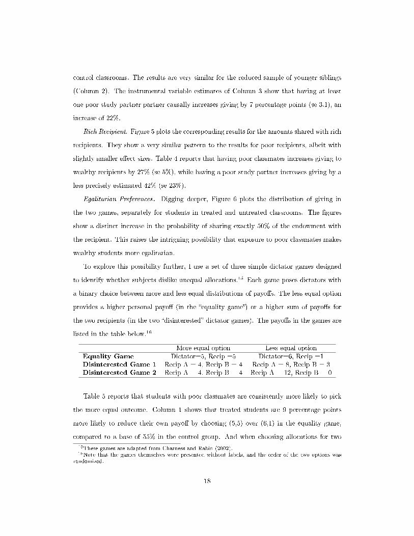
To explore this possibility further, I use a set of three simple dictator games designed

to identify whether subjects dislike unequal allocations.15 Each game poses dictators with

a binary choice between more and less equal distributions of payo�s. The less equal option

provides a higher personal payo� (in the �equality game�) or a higher sum of payo�s for

the two recipients (in the two �disinterested� dictator games). The payo�s in the games are

listed in the table below.16

More equal option Less equal optionEquality Game Dictator=5, Recip =5 Dictator=6, Recip =1Disinterested Game 1 Recip A = 4, Recip B = 4 Recip A = 8, Recip B = 3Disinterested Game 2 Recip A = 4, Recip B = 4 Recip A = 12, Recip B = 0

Table 5 reports that students with poor classmates are consistently more likely to pick

the more equal outcome. Column 1 shows that treated students are 9 percentage points

more likely to reduce their own payo� by choosing (5,5) over (6,1) in the equality game,

compared to a base of 55% in the control group. And when choosing allocations for two

15These games are adapted from Charness and Rabin (2002).16Note that the games themselves were presented without labels, and the order of the two options was

randomized.

18

anonymous recipients (holding their own payo� �xed) in the disinterested dictator games,

they are 12 percentage points more likely to choose (4,4) over (8,3) and 14 percentage points

more likely to pick (4,4) over (12,0).

Considering the set of dictator game results together, I conclude that having poor class-

mates does not simply make students more charitable towards the poor. Instead, it makes

them more generous overall, and in particular makes them exhibit more egalitarian prefer-

ences over monetary payo�s. This is an important point, suggesting that interacting with

poor children in school does not just make students more favorably inclined towards the

poor. Rather, it changes more fundamental preferences regarding fairness.

The dictator game measures were entirely independent of the �eld observations of volun-

teering behavior described previously. Putting together the �ndings of increased generosity

in the lab and increased volunteering in the �eld thus substantially strengthens my conclu-

sion that being exposed to poor children in school makes wealthy students more prosocial.

5 Social Interactions and Discrimination

Discrimination is a pervasive and important phenomenon in labor markets (Goldin and

Rouse 2000, Bertrand and Mullainathan 2004), law enforcement (Persico 2009), residential

location choice (Becker and Murphy 2009) and other contexts. Theories of discrimination

are of two main types: taste-based discrimination, re�ecting an innate animosity towards

individuals from a particular group (Becker 1957), and statistical discrimination, which

results from imperfect information about productivity or ability (Phelps 1972, Arrow 1973,

Aigner and Cain 1977).

Tastes for social interactions provide a natural foundation for taste-based discrimination.

But social interaction models also explain features of residential patterns (Schelling 1971),

collective action (Granovetter, 1978), job search (Beaman and Magruder 2012) and the

marriage market. Changes in willingness to interact with members of other social groups

are therefore a potentially important outcome of diversity in schools. Indeed, theory suggests

that even small changes in these tastes can lead to large di�erences in aggregate outcomes,

19

since social interaction models often feature multiple equilibria (Card et al. 2008).

In this section, I estimate how having poor classmates in school a�ects rich students'

willingness to socially interact and work with other poor children in teams, or conversely to

discriminate against them. I design two novel experiments to measure these outcomes. The

�rst is a team selection �eld experiment designed to estimate taste-based discrimination

using exogenous variation in the price of discrimination. The second experiment elicits

students �willingness to play� - the cost they attach to attending a play date with poor

children.

5.1 Team-Selection Field Experiment

Design. The main idea of the team-selection experiment is to create a tradeo� for wealthy

students between choosing a high ability teammate (and thus increasing their own expected

payo�) versus choosing a lower-ability teammate with whom they would prefer to socialize.

The team task I used in the experiment was a relay race, a task which was familiar to all

the students, and in which ability is easily revealed through times in individual sprints.

In addition to running the relay race together, participants were required to spend time

socializing with their teammates.

The experiment was conducted on the sidelines of a sports meet featuring athletes from

two elite private schools - one a treatment school, and the other a control school. The

participants in the experiment were not the athletes themselves, but were instead drawn

from the large contingents of students who were present to support their teams. Note

that attendance in this supporting role was compulsory for students in both schools; the

attendees were not a selected set of cheerleaders. In addition to students from the two

elite private schools, I invited selected students from a public school catering to relatively

poor students to participate in the experiment. These students were selected for having a

particular interest in athletics.

The experiment proceeded in four stages.

Randomization. First, students were randomized to di�erent sessions (separately by

gender) with varying stakes for winning the subsequent relay race - either Rs. 500, Rs. 200

20

or Rs. 50 per teammate for winning the race. 500 rupees are approximately a month's

pocket money for the oldest students in the sample, so the stakes are substantial. Within

each session, students were asked to mix and introduce themselves to each other for about

�fteen minutes. This ensured that students were able to accurately identify the di�erence

in the social groups that the various participants belonged to. School uniforms made group

membership salient, and debrie�ng suggested that students were quickly able to identify

that the students from the public school were relatively poor, while the students from the

private schools were wealthy. At the end of this phase, the following three stages were

described to the students, and the experiment proceeded.

Ability Revelation and Team Selection. Students watched a series of one-on-one sprints,

designed to reveal each runner's ability. In most cases, one runner was from the public

school, while the other was from one of the private schools. However, some pairs included

two students from private schools, or two from the public school. After each sprint, the rank

(�rst or second) and times of the two runners were announced.

Decision Stage. After each such ability revelation sprint, students privately chose on a

worksheet which of the two students they would like to have in their two-person team for a

relay race. After the sprints were complete, six students were picked at random to participate

in the relay race, and one of their choices was randomly selected for implementation.

Relay Race and Socializing with Teammate. The relay races were conducted and rewards

were distributed as promised. After the rewards were distributed, students were required

to spend two hours socializing with their teammate. They were provided with board games

and could also use playground equipment. However, they were not permitted to play in

larger groups. This part of the experiment was described to the participants in advance,

so they knew that their interactions with their selected teammate would exceed the few

minutes spent on the relay race itself.

Reduced Form Results. The �rst reduced form �nding is signi�cant discrimination

against the poor on average. I classify a wealthy student as having discriminated against

the poor if he or she chooses a lower ability (i.e. slower) rich student from another school

21

over a higher ability poor student from the public school.17 Averaging over the di�erent

reward conditions, participants discriminate 19% of the time. These are not just mistakes,

since the symmetric mistake of �discriminating� against a rich student occurs only 3% of

the time. And when participants are choosing between two runners from the same (other)

school, they pick the slower runner only 2% of the time. Thus, only poor students competing

against rich students are systematically discriminated against.

The second �nding is that discrimination decreases as the stakes increase. In the control

school, 35% of choices exhibit discrimination against the poor in the Rs. 50 condition, but

this falls to 27% when the reward is Rs. 200, and only 5% in the highest stakes condition

of Rs. 500. This result is shown by the solid line in Figure 7, which I interpret as a demand

curve for discrimination.

The third and most important �nding is a reduction in discrimination from having poor

classmates and study partners. Figure 7 shows that for each level of stakes, wealthy students

with poor classmates are less likely to discriminate against the poor. In addition, the slope of

the demand curve for discrimination is higher for students with poor classmates. Figure 8(a)

depicts the di�erence-in-di�erences estimates graphically by plotting rates of discrimination

by school and grade. In the treatment school, discrimination is substantially lower than

in the control school in the treated grades 2 and 3, but not in grades 4 and 5. Figure

8(b) instead depicts the reduced form of the IV strategy, plotting rates of discrimination

by whether the student has a name alphabetically adjacent to a poor students. Consistent

with the di�erence-in-di�erences result, the �gure shows that students with names close to a

poor student (and therefore a higher likelihood of having a poor study partner) discriminate

less.

Regression estimates are reported in Table 6. Column 1 shows that having a poor

classmate reduces discrimination by 12 percentage points (se 5).18 This e�ect is comparable

to the 11 percentage point reduction in discrimination caused by increasing the stakes from

17I do not consider a choice to be discriminatory if it involves choosing ones own schoolmate over ahigher-ability poor student, since participants may prefer to partner with children they already know.

18Since the discrimination experiment has wealthy students from only two schools, I do not attempt tocluster standard errors at the school level. Instead, I report unclustered standard errors and, as a robustnesscheck, cluster at the school-by-grade level (8 clusters) using the wild cluster bootstrap method.

22

Rs. 50 to Rs. 200 (an increase of about $3). Column 2 shows that having poor classmates

has the biggest e�ect on discrimination in the lowest stakes condition (a 25 percentage

point reduction). Column 3 reports the IV result that having a poor study partner reduces

discrimination by 14.7 percentage points (se 8.8).19

The observed behavior is more consistent with taste-based discrimination rather than

statistical discrimination. When a separate sample of students is asked which of the two

runners is more likely to be in the winning relay race, 98% pick the faster student. This

implies that many students prefer a wealthy teammate even though they believe he makes

them less likely to win, a fact inconsistent with a simple model of statistical discrimination.

This is not surprising, since the experiment was designed with the intention of measuring

taste-based discrimination. The clear signals of ability provided by the sprints additionally

make statistical discrimination unlikely. And the fact that participants are forced to actually

spend time socializing with their teammates - as is often the case when hiring colleagues or

employees - provides a natural setting for taste-based discrimination.

Since the experiment does not simulate a market with a wage o�ered to teammates,

I cannot directly test the classic prediction of taste-based discrimination that only the

marginal employer's tastes matter. However, the fact that about 35% of control students

discriminate in the low stakes condition suggests that at least a third of wealthy students

dislike having a poor teammate (relative to a wealthy teammate).

Model and Structural Estimation. The reduced form results provide evidence of

a reduction in discrimination. But they do not inform us of the precise magnitude of the

distaste that wealthy students have for partnering and socializing with a poor child, nor

how much this is changed by having poor classmates. In order to estimate these quantities,

I structurally estimate a simple model of discrimination.

Model . Suppose the decision-maker has expected utility:

Ut = ptM + St (3)

19The treatment school uses alphabetic order to assign study partners. Since the sample for this experi-ment does not include any other treatment schools which do not use such a rule, I directly use alphabeticadjacency to a poor student as the instrument for having a poor student in one's study group.

23

where pt is the probability of winning the race with teammate t, M is the monetary

reward for winning the race and St is the utility from socially interacting with teammate t.

I assume that teammates are of two types, t ∈ {R,P}, where R denotes a rich student and

P denotes a poor student.

Then, she chooses the rich teammate if

pRM + SR > pPM + SP

⇔ SR − SP > (pP − pR)M

In the absence of a particular distaste for having a poor teammate, SP = SR. And in the

absence of statistical discrimination, rich and poor students with the same performance in

the sprint would be perceived to be equally able, pP = pR. De�ne Dpoor ≡ SR − SP as the

distaste for interacting with a poor student (relative to a rich student), and δpoor ≡ pP −pR

as the perceived increase in probability of winning from having a poor teammate, provided

the poor student won the ability-revelation sprint. Then, the decision-maker discriminates

against a poor student if:

Dpoor > δpoorM (4)

Similarly, in the case where the rich student wins the sprint, we can de�ne the increase

in probability of winning from choosing the rich teammate, δrich.

In order to estimate the model, I impose the following distributional assumption: Dpoor

is distributed normally with mean µTD and standard deviation σTD, separately for students

from treated classrooms (T = 1) and untreated classrooms (T = 0). Consistent with the

fact that 98% of students state that the winner of the ability sprint is more likely to win

the relay race (regardless of whether the winner was rich or poor), I additionally impose the

assumption of no statistical discrimination, δpoor = δrich ≡ δ.

Then, the parameters to be estimated are: (i) µ1D and µ0

D, the average distaste for

24

having a poor teammate amongst students with and without poor classmates, respectively;

(ii) σ1D and σ0

D , the standard deviations of the distribution of distaste; (iii) δ, the increase

in probability of winning from choosing the teammate who won the ability-revelation sprint.

I estimate these parameters using a classical minimum distance estimator. Speci�cally,

the estimator solves Minθ (m(θ)− m̂)′W (m(θ)− m̂), where m̂ is a vector of the empiri-

cal moments and m(θ) is the vector of theoretically predicted moment for parameters θ.

The weighting matrix W is the diagonalized inverse of the variance of each moment; more

precisely estimated moments receive greater weight in the estimation.

The moments for the estimation are the following: (i) The probability of discriminating

against a higher-ability poor student, separately by stakesM ∈ {50, 200, 500} and treatment

status T ∈ {0, 1}, and (ii) The probability of discriminating against a higher-ability rich

student, by stakes M and treatment status T . The empirical moments are simply shares

of students observed to discriminate in each condition, estimated by an uncontrolled OLS

regression.

Identi�cation. All 5 parameters are jointly identi�ed using the 12 moments. The in-

tuition for the identi�cation is straightforward. Conditional on δ, the exogenous variation

in the stakes M pins down the mean µD and standard deviation σD of the distribution of

distaste D. Conditional on the distribution of D, the perceived increase in probability of

winning from choosing a high-ability teammate (δ), is identi�ed from comparing the prob-

abilities of choosing (say) the poor student when he wins versus loses the ability-revelation

sprint.

Estimates. The lower panel in Table 7 reports the empirical and �tted values of the

moments. The model overall does a good job of �tting the moments, with the exception

of slightly over-predicting discrimination against the poor in the lowest stakes condition.

Table 7 also reports the structural estimates of the parameters. The perceived increase

in probability of winning from choosing a high-ability teammate is imprecisely estimated,

δ = 0.08 (se 0.1). Students without poor classmates are estimated to feel an average distaste

for having a poor teammate of µ0D =Rs. 37 (se Rs. 4.4), with a standard deviation σ0

D =

Rs. 6 (se Rs. 1.9). In contrast, treated students are estimated to have a substantially

25

lower distaste of µ1D =Rs. 26 (se Rs. 4.8) and a similar standard deviaion, σ1

D = Rs. 5 (se

Rs. 2.1). The di�erence in average distaste of Rs. 11 is signi�cant at the 10% level, and

constitutes a 30% reduction relative to students without poor classmates.

5.2 Willingness to Play

To shed more light on the observed reduction in discrimination in the team-selection experi-

ment, I directly test wealthy students' tastes for socially interacting with poor children. I do

so by inviting them to play dates at neighborhood schools for poor children. The play dates

were motivated as an opportunity to make new friends, and involved two hours of games

and playground activities. In order to measure tastes, I elicited incentivized measures of

wealthy students' willingness to accept to attend these play dates. I �nd that having poor

classmates in school makes wealthy students substantially more willing to play with other

poor children.

Protocol. First, students were informed in school about the play dates. The play date was

presented to them as an opportunity to make new friends in their neighborhood. The host

school was named and described, and the experimenter showed the students a photograph

of the school. The play dates all occurred on a weekend morning, and the students were

informed about them approximately two weeks before the play date.

After answering students questions about the planned play dates, I elicited their will-

ingness to accept - the payment they required - to attend the play date.20 I employed a

simple Becker-Degroot-Marschak mechanism, where students were presented with a decision

sheet showing possible levels of payments for attending the play date. For each such price

level, they were asked to indicate whether they would like to attend the play date. Then, a

numbered ball was drawn from a bag, and their decision corresponding to that price was im-

plemented. In particular, if they had indicated they would like to attend for the drawn price,

their name was written down on a list, and they were provided an invitation form to take

20Pilot work revealed that students generally �nd the play dates unattractive � nearly all students ex-pressed a negative willingness to pay. This is unsurprising, given that the play dates were held on weekends,which are surely a precious part of a child's week. The opportunity cost of attending anecdotally includedwatching television and playing with existing friends.

26

home to their parents.21 The entire procedure was �rst explained to the students verbally,

and then they played three practice rounds, at which point they appeared to understand

the decision well.

Results. The key �nding is that students become more willing to socialize with poor

children if they already have poor classmates. Figure 9 shows the results of the two identi-

�cation strategies graphically. Panel (a) plots average willingness to accept by school type

(control, treatment and delayed treatment) and grade. For treatment schools, willingness

to accept is lower than control schools only in the treated grades 2 and 3, but not in the

untreated grades 4 and 5. A similar pattern is visible for delayed treatment schools, in which

only grade 3 is treated. A lower willingness to accept indicates greater willingness to socially

interact with poor children. Figure 10 plots the resulting supply curves for attending the

play date, separately for students with and without poor classmates.

Figure 9(b) depicts the IV strategy graphically, by plotting average willingness to accept

by whether the wealthy student has a name alphabetically adjacent to any poor children.

We see that having an alphabetic neighbor only increases willingness to play in schools which

use the alphabetic assignment rule. This suggests that personally interacting with a poor

student through assignment to a common study group reduces a wealthy students' distaste

for interacting with other poor children.

Finally, Table 8 reports numerical estimates of the e�ects, using the speci�cations dis-

cussed in Section 3. I �nd that having poor classmates decreases willingness to accept (i.e.

increases willingness to play) by Rs. 7 (se 1.1) on a base of Rs. 37, a decrease of 19%. The

e�ect is highly signi�cant (p<0.01) even when clustering standard errors at the school level,

and the result is similar in the restricted sample of younger siblings. Having a poor study

partner reduces willingness to accept by 24% (se 9%).

In contrast, I �nd no e�ects on willingness to attend play dates with rich students.

In August 2013, I conducted a parallel experiment in a smaller sample as a placebo test.

Students now had the opportunity to spend two hours playing with other wealthy students

21Parents, of course, had the ability to veto their childrens' choice to attend the play date, and didso in about 35% of cases. Since I wish to isolate the child's tastes rather than the parents, I use theelicited willingness to pay (or accept) as the outcome measure. Using actual attendance of play dates as analternative outcome, I �nd similar but muted e�ects.

27

from a control private school. While the estimates are less precise due to a smaller sample

size, Appendix Table 1 reports no average e�ect on willingness to play with rich students.

6 Academic Outcomes

One concern with integrating disadvantaged students into elite schools is that wealthy stu-

dents' academic outcomes may su�er as a result. This concern is motivated by the large

literature studying peer e�ects in education, which has sometimes found substantial peer

e�ects (Hoxby 2000, Hanushek et al. 2003) and at other times no evidence that peers a�ect

test scores (Angrist and Lang 2004, Imberman et al. 2009). Classroom disruptions by poorly

disciplined students have been proposed to an key mechanism underlying any negative ef-

fects (Lazear 2001, Lavy and Schlosser 2011, Figlio 2007). Indeed, principals in the schools

I studied reported being particularly concerned about classroom disruptions and learning.

In this section, I therefore turn attention to estimating the impact of poor students on the

learning and classroom discipline of their wealthy peers.

6.1 Learning

To measure e�ects on learning, I conduct simple tests of learning in English, Hindi and

Math. With the assistance of teachers in a non-sample school, I �rst assembled a master list

of questions from standard textbooks for grades 1 through 7. Students in each grade were

asked to answer a set of questions considered appropriate for their grade, and a smaller set

of questions at lower and higher grade levels. The test was designed to be quick and easy

to implement, and therefore provides a somewhat coarse measure of learning. Nonetheless,

it provides comparable test scores across di�erent schools in the absence of any existing

system of standardized testing in primary schools. I normalize the test score in order to

provide standardized e�ect sizes.

I �nd that poor students do worse than rich students on average, but with substantial

heterogeneity. Poor students score 0.32 standard deviations (s.d.) worse than wealthy

students in English, 0.12 s.d. worse in Hindi and 0.24 s.d. worse in Math. The lower

28

average learning levels of poor students make the possibility of negative peer e�ects very

real. But the variance in poor students' test scores is similar to that of wealthy students;

there is thus plenty of overlap in the distributions of academic achievement. For example,

poor students have weakly higher scores than 40% of their wealthy study partners even in

English.

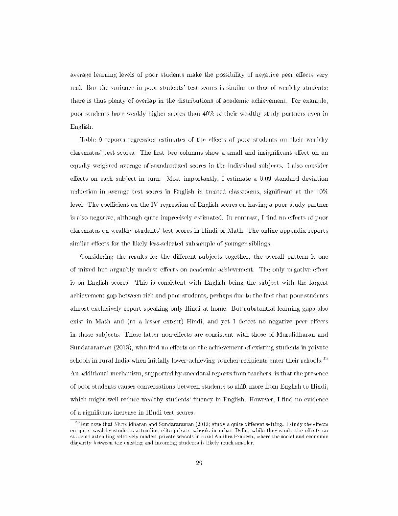
Table 9 reports regression estimates of the e�ects of poor students on their wealthy

classmates' test scores. The �rst two columns show a small and insigni�cant e�ect on an

equally weighted average of standardized scores in the individual subjects. I also consider

e�ects on each subject in turn. Most importantly, I estimate a 0.09 standard deviation

reduction in average test scores in English in treated classrooms, signi�cant at the 10%

level. The coe�cient on the IV regression of English scores on having a poor study partner

is also negative, although quite imprecisely estimated. In contrast, I �nd no e�ects of poor

classmates on wealthy students' test scores in Hindi or Math. The online appendix reports

similar e�ects for the likely less-selected subsample of younger siblings.

Considering the results for the di�erent subjects together, the overall pattern is one

of mixed but arguably modest e�ects on academic achievement. The only negative e�ect

is on English scores. This is consistent with English being the subject with the largest

achievement gap between rich and poor students, perhaps due to the fact that poor students

almost exclusively report speaking only Hindi at home. But substantial learning gaps also

exist in Math and (to a lesser extent) Hindi, and yet I detect no negative peer e�ects

in those subjects. These latter non-e�ects are consistent with those of Muralidharan and

Sundararaman (2013), who �nd no e�ects on the achievement of existing students in private

schools in rural India when initially lower-achieving voucher-recipients enter their schools.22

An additional mechanism, supported by anecdotal reports from teachers, is that the presence

of poor students causes conversations between students to shift more from English to Hindi,

which might well reduce wealthy students' �uency in English. However, I �nd no evidence

of a signi�cant increase in Hindi test scores.

22But note that Muralidharan and Sundararaman (2013) study a quite di�erent setting. I study the e�ectson quite wealthy students attending elite private schools in urban Delhi, while they study the e�ects onstudents attending relatively modest private schools in rural Andhra Pradesh, where the social and economicdisparity between the existing and incoming students is likely much smaller.

29

6.2 Discipline

To measure classroom discipline, I ask teachers to report whether each student has been

cited for any disciplinary infractions in the past six months23. I �nd that 22% of wealthy

students have been cited for the use of inappropriate language (that is, swearing) in school,

but only about 6% are cited for disruptive or violent behavior. Poor students are no more

likely than rich students to be disruptive in class, but they are 12 percentage points more

likely to be reported for using o�ensive language.

Table 10 reports regression estimates of the e�ects of poor students on disciplinary

infractions by their wealthy classmates. The results suggest that having poor classmates

increases the share of wealthy students reported for using inappropriate language by 7.5

percentage points (se 3.7). Having a poor study partner causes an even larger increase of 10

percentage points (se 6), an increase of about 45%. In contrast, I �nd precisely estimated

zero e�ects on the likelihood of being cited for disruptive or violent behavior.

The �nding that poor students do not make their wealthy classmates more disruptive �

and indeed are no more disruptive than wealthy students themselves � is consistent with the

absence of negative peer e�ects on Hindi and Math scores. In the context I study, concerns

about diversity a�ecting test scores through indiscipline appear to be unwarranted. In

contrast, the e�ects on inappropriate language use are substantial, although likely without

implication for learning and future academic achievement.

7 Conclusion

In this paper, I exploit a natural experiment in education policy in India to estimate how

greater economic diversity in classrooms a�ects wealthy students. I assemble a variety

of evidence from �eld and lab experiments, administrative data and tests of learning to

reach three main �ndings. The �rst �nding is that having poor classmates makes wealthy

students more prosocial and concerned about equality, and thus more generous towards

others. The second �nding is that wealthy students become more willing to socially interact

23This question was asked at the end of the academic year

30

with poor children outside school, and thus exhibit less taste-based discrimination against

the poor. The third �nding is of mixed but overall modest impacts on academic outcomes,

with negative e�ects on English language learning but no e�ect on Hindi or Math. Thus,

my overall conclusion is that increased diversity in the classroom led to large and arguably

positive impacts on social preferences and behaviors, at the cost of negative but modest

impacts on academic outcomes.

One implication of these �ndings is that school policies involving a�rmative action,

desegregation and tracking should be evaluated not only on learning outcomes - which are

of unarguable importance - but also on other economically important outcomes related to

social behaviors. More generally, my �ndings support the view that increased interactions

across social groups, perhaps especially in childhood, can improve inter-group behaviors.

This �nding has implications for diverse and polarized societies, where the costs of social

divisions are thought to be high. Finally, my �ndings are of relevance to the planned

expansion of this policy across India over the next few years.

One limitation of this paper is that due to the recency of the policy experiment, it

does not study important long-term outcomes and behaviors such as political beliefs, social

interactions as adults, and marriage market choices. Another limitation is the very particular

nature of the sample - wealthy students in elite private schools in Delhi. Finally, this paper

does not examine the e�ects on poor students of attending elite private schools, which might

have profound consequences for their academic achievement and life outcomes. In ongoing

and future work, I hope to address these shortcomings, as well as examine other aspects of

the impacts of diversity in schools.

31

References

[1] Aigner, D. J., and Cain, G. G. Statistical theories of discrimination in labor

markets. Industrial and Labor relations review 30, 2 (1977), 175�187.

[2] Akerlof, G. A. Gift exchange and e�ciency-wage theory: Four views. The American

Economic Review 74, 2 (1984), 79�83.

[3] Alesina, A., and Glaeser, E. Fighting poverty in the us and europe: A world of

di�erence. OUP Catalogue (2005).

[4] Alesina, A., and Perotti, R. Income distribution, political instability, and invest-

ment. European Economic Review 40, 6 (1996), 1203�1228.

[5] Allport, G. W. The nature of prejudice. Addison-Wesley, 1954.

[6] Almås, I., Cappelen, A. W., Sørensen, E. Ø., and Tungodden, B. Fairness

and the development of inequality acceptance. Science 328, 5982 (2010), 1176�1178.

[7] Andreoni, J. Toward a theory of charitable fund-raising. Journal of Political Economy

106, 6 (1998), 1186�1213.

[8] Andreoni, J., and Miller, J. Giving according to garp: An experimental test of

the consistency of preferences for altruism. Econometrica 70, 2 (2002), 737�753.

[9] Angrist, J. D., and Lang, K. Does school integration generate peer e�ects? evidence

from boston's metco program. The American Economic Review 94, 5 (2004), 1613�1634.

[10] Arrow, K. The theory of discrimination. In Discrimination in Labor Markets,

O. Ashenfelter and A. Rees, Eds. Princeton University Press, 1973.

[11] Bandiera, O., Barankay, I., and Rasul, I. Social preferences and the response to

incentives: Evidence from personnel data. The Quarterly Journal of Economics 120, 3

(2005), 917�962.

[12] Bardhan, P., Ghatak, M., and Karaivanov, A. Wealth inequality and collective

action. Journal of Public Economics 91, 9 (2007), 1843�1874.

[13] Becker, G. S. The economics of discrimination. University of Chicago press, 1957.

32

[14] Becker, G. S., and Murphy, K. M. Social economics: Market behavior in a social

environment. Harvard University Press, 2009.

[15] Benz, M., and Meier, S. Do people behave in experiments as in the �eld? evidence

from donations. Experimental Economics 11, 3 (2008), 268�281.

[16] Bertrand, M., and Mullainathan, S. Are emily and greg more employable than

lakisha and jamal? a �eld experiment on labor market discrimination. The American

Economic Review 94, 4 (2004), 991�1013.

[17] Boisjoly, J., Duncan, G. J., Kremer, M., Levy, D. M., and Eccles, J. Em-

pathy or antipathy? the impact of diversity. The American Economic Review 96, 5

(2006), 1890�1905.

[18] Buchmann, C., and Hannum, E. Education and strati�cation in developing coun-

tries: A review of theories and research. Annual review of sociology (2001), 77�102.

[19] Burns, J., Corno, L., and La Ferrara, E. Does interaction a�ect racial prejudice

and cooperation? evidence from randomly assigned peers in south africa. Unpublished

working paper (2013).

[20] Cameron, A. C., Gelbach, J. B., and Miller, D. L. Bootstrap-based improve-

ments for inference with clustered errors. The Review of Economics and Statistics 90,

3 (2008), 414�427.

[21] Card, D., Mas, A., and Rothstein, J. Tipping and the dynamics of segregation.

The Quarterly Journal of Economics 123, 1 (2008), 177�218.

[22] Charles, K. K., and Guryan, J. Studying discrimination: Fundamental challenges

and recent progress. Tech. rep., National Bureau of Economic Research, 2011.

[23] Charness, G., and Rabin, M. Understanding social preferences with simple tests.

The Quarterly Journal of Economics 117, 3 (2002), 817�869.

[24] Easterly, W., and Levine, R. Africa's growth tragedy: policies and ethnic divisions.

The Quarterly Journal of Economics 112, 4 (1997), 1203�1250.

33

[25] Edlin, A. S., Gelman, A., and Kaplan, N. Voting as a rational choice: Why and

how people vote to improve the well-being of others. Rationality and society 1 (2007).

[26] Esteban, J., and Ray, D. Linking con�ict to inequality and polarization. The

American Economic Review 101, 4 (2011), 1345�1374.

[27] Fehr, E., Bernhard, H., and Rockenbach, B. Egalitarianism in young children.

Nature 454, 7208 (2008), 1079�1083.

[28] Figlio, D. N. Boys named sue: Disruptive children and their peers. Education 2, 4

(2007), 376�394.

[29] Finan, F., and Schechter, L. Vote-buying and reciprocity. Econometrica 80, 2

(2012), 863�881.

[30] Fisman, R., Jakiela, P., and Kariv, S. How did the great recession impact social

preferences? Unpublished working paper (2012).

[31] Fisman, R., Kariv, S., and Markovits, D. Exposure to ideology and distributional

preferences. Unpublished paper (2009).

[32] Goldin, C., and Rouse, C. Orchestrating impartiality: The impact of. The American

Economic Review 90, 4 (2000), 715�741.

[33] Granovetter, M. Threshold models of collective behavior. American journal of

sociology (1978), 1420�1443.

[34] Hanushek, E. A., Kain, J. F., Markman, J. M., and Rivkin, S. G. Does peer

ability a�ect student achievement? Journal of Applied Econometrics 18, 5 (2003),

527�544.

[35] Hattie, J. A. Classroom composition and peer e�ects. International Journal of

Educational Research 37, 5 (2002), 449�481.

[36] Hoffman, E., McCabe, K., and Smith, V. L. Social distance and other-regarding

behavior in dictator games. The American Economic Review 86, 3 (1996), 653�660.

[37] Hoxby, C. Peer e�ects in the classroom: Learning from gender and race variation.

Tech. rep., National Bureau of Economic Research, 2000.

34

[38] Imberman, S., Kugler, A. D., and Sacerdote, B. Katrina's children: evidence

on the structure of peer e�ects from hurricane evacuees. Tech. rep., National Bureau

of Economic Research, 2009.

[39] Jakiela, P., Miguel, E., and Te Velde, V. L. You've earned it: Combining �eld

and lab experiments to estimate the impact of human capital on social preferences.

Tech. rep., National Bureau of Economic Research, 2010.

[40] Karlan, D. S. Using experimental economics to measure social capital and predict

�nancial decisions. American Economic Review (2005), 1688�1699.

[41] Karsten, S. School segregation. In Equal Opportunities?: The Labour Market Inte-

gration of the Children of Immigrants. OECD Publishing, 2010.

[42] Lavy, V., and Schlosser, A. Mechanisms and impacts of gender peer e�ects at

school. American Economic Journal: Applied Economics 3, 2 (2011), 1�33.

[43] Lazear, E. P. Educational production. The Quarterly Journal of Economics 116, 3

(2001), 777�803.

[44] List, J. A. The nature and extent of discrimination in the marketplace: Evidence

from the �eld. The Quarterly Journal of Economics 119, 1 (2004), 49�89.

[45] Miguel, E., and Gugerty, M. K. Ethnic diversity, social sanctions, and public

goods in kenya. Journal of Public Economics 89, 11 (2005), 2325�2368.

[46] Mobius, M. M., and Rosenblat, T. S. Why beauty matters. The American Eco-

nomic Review (2006), 222�235.

[47] Muralidharan, K., and Sundararaman, V. The aggregate e�ect of school choice:

Evidence from a two-stage experiment in india. 2013.

[48] Persico, N. Racial pro�ling? detecting bias using statistical evidence. Annu. Rev.

Econ. 1, 1 (2009), 229�254.

[49] Pettigrew, T. F., and Tropp, L. R. A meta-analytic test of intergroup contact

theory. Journal of personality and social psychology 90, 5 (2006), 751.

35

[50] Phelps, E. S. The statistical theory of racism and sexism. The american economic

review 62, 4 (1972), 659�661.

[51] Sacerdote, B. Peer e�ects in education: How might they work, how big are they and

how much do we know thus far? Handbook of the Economics of Education 3 (2011),

249�277.

[52] Schelling, T. C. Dynamic models of segregation. Journal of mathematical sociology

1, 2 (1971), 143�186.

[53] Schofield, J. W. School desegregation and intergroup relations: A review of the

literature. Review of research in education 17 (1991), 335�409.

[54] Van Ewijk, R., and Sleegers, P. The e�ect of peer socioeconomic status on student

achievement: A meta-analysis. Educational Research Review 5, 2 (2010), 134�150.

[55] Voors, M. J., Nillesen, E. E., Verwimp, P., Bulte, E. H., Lensink, R., and

Van Soest, D. P. Violent con�ict and behavior: a �eld experiment in burundi. The

American Economic Review 102, 2 (2012), 941�964.

36

39

Figure 1. Program eligibility and the household income distribution in Delhi

Note: This graph is based on the household consumption distribution reported in NSS-2010, with

consumption amount converted to income levels using the ratio of household income to household

consumption for urban Indian households reported in IHDS-2005.

40

Figure 2. First Stage of Instrumental Variable

Note: Having a name alphabetically adjacent to a poor student predicts having a poor student

in one’s study group, but only in the schools which explicitly use alphabetic ordering

41

Figure 3. Volunteering for Charity

Note: The top panel plots the share of wealthy students who participate in voluntary charitable

fundraising activities in school, separately by type of school. Error bars plot 95% confidence intervals

(unclustered).

The bottom panel plots share volunteering by whether the subject has a name alphabetically adjacent to

any poor students, separately by whether schools use alphabetic order to assign study groups.

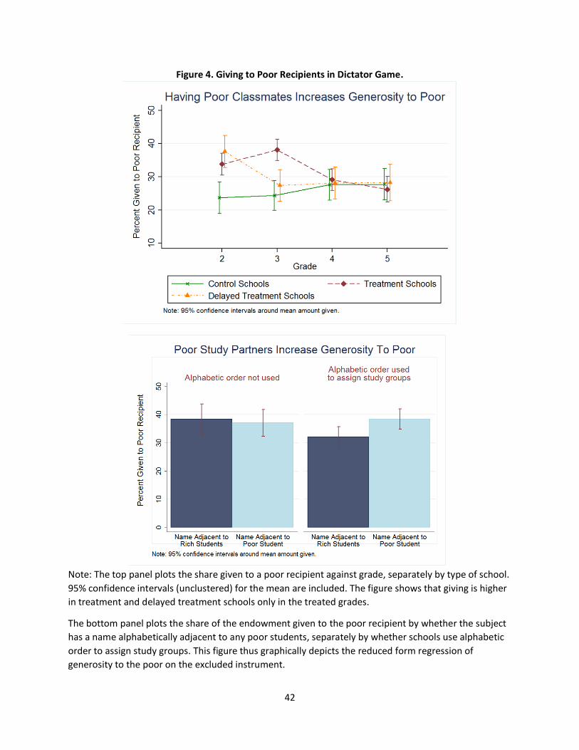
42

Figure 4. Giving to Poor Recipients in Dictator Game.

Note: The top panel plots the share given to a poor recipient against grade, separately by type of school.

95% confidence intervals (unclustered) for the mean are included. The figure shows that giving is higher

in treatment and delayed treatment schools only in the treated grades.

The bottom panel plots the share of the endowment given to the poor recipient by whether the subject

has a name alphabetically adjacent to any poor students, separately by whether schools use alphabetic

order to assign study groups. This figure thus graphically depicts the reduced form regression of

generosity to the poor on the excluded instrument.

43

Figure 5. Giving to Wealthy Recipients in Dictator Game.

Note: The top panel plots the share given to a wealthy recipient against grade, separately by type of

school. 95% confidence intervals (unclustered) for the mean are included.

The bottom panel plots the share of the endowment given to the poor recipient by whether the subject

has a name alphabetically adjacent to any poor students, separately by whether schools use alphabetic

order to assign study groups.

44

Figure 6. Distribution of Giving in Treated and Untreated Classrooms

Note: The top panel shows the distribution of giving by wealthy students to poor recipients, separately

for whether they have poor classmates (red bars) or not (blue bars). The bottom panel shows the same

results for giving to wealthy recipients instead of poor recipients.

45

Figure 7. Demand Curve for Discrimination

Notes: This graph plots the share of wealthy students who discriminate against the poor (on the y axis)

by the stakes of the decision, separately by whether the student has poor classmates (dotted red line) or

not (solid green line). A student is classified as having discriminated against the poor if he chooses a

lower-ability rich student over a higher-ability poor student.

46

Figure 8. Discrimination Against the Poor

Notes: The top panel plots the share of wealthy students who discriminate against the poor (on the y

axis) by grade (on the axis), separately by school type. The control school is represented by the solid

green line, while the treatment school is represented by the dotted red line. Error bars plot 95%

confidence intervals (unclustered).

The bottom panel plots discrimination rates by whether the participant has a name alphabetically

adjacent to any poor students, only for the treatment school.

47

Figure 9. Willingness to Play

Note: The top panel plots wealthy students’ average Willingess To Accept a play date with poor children,

separately by type of school. Error bars plot 95% confidence intervals (unclustered).

The bottom panel plots “willingess to play” by whether the subject has a name alphabetically adjacent

to any poor students, separately by whether schools use alphabetic order to assign study groups.

48

Figure 10. Supply Curve for Attending Play Date

Note: This graph plots the share of wealthy students willing to attend the play date with poor children

(on the y axis) for each given level of payment for attending the play date (on the x axis). The solid

green line represents this supply curve for wealthy students without poor classmates, while the dotted

red line represents wealthy students who do have poor classmates.

47

Table 1. First Stage of IV

Dependent Variable:

Indicator for having at least one poor student in one’s study groups (1)

Instrument Has Poor Study Partner

(Name Adjacent to Poor Student) x

(School Uses Alphabetic Rule)

0.519***

(0.0808)

Constant 0.456***

(0.0793)

N 677

F-Statistic 41.25

Note: Standard errors in parentheses. This table reports the results from regressing an indicator for

whether the student has a poor study group partner on the excluded instrument, school and grade

dummies, and a vector of second stage control variables. The F statistic reports results of a Wald

test of a zero coefficient on the instrument * p < 0.10, ** p < 0.05, *** p < 0.01

48

Table 2. Volunteering for Charity

Dependent Variable:

Indicator for Volunteering for Charity (1) (2) (3) (4)

Specification:

Sample:

DiD

Full Sample

DiD

Younger Sibs

IV

Treated Class

DiD+IV

Full Sample

Treated Classroom 0.105***

(0.0244)

0.0715**

(0.0305)

-0.0409

(0.0766)

Has Poor Study Partner

0.130

(0.0866)

0.208**

(0.0881)

Controls Yes Yes Yes Yes

Fixed Effects School, Grade School, Grade Classroom School, Grade

p-value (CGM) < 0.01 0.06 . .

Control Mean 0.242 0.220 0.245 0.242

Control SD 0.428 0.414 0.431 0.428

N 2017 1143 677 2017

Note. Standard errors in parentheses. This table reports results from linear probability models for the likelihood

of volunteering for a charity. Col 1 reports a difference-in-differences estimates of the effect of having poor

students in one's classroom, with standard errors clustered at the school-by-grade level. The p-value reported in

the table instead is calculated using clustering at the school level (k=14) using Cameron, Gelbach and Miller's

wild-cluster bootstrap. Col 2 reports the same specification as Col 1, but restricts the sample to students who have

older siblings enrolled in the same school. Col 3 reports IV estimates of the effect of having a poor study partner,

and presents robust standard errors. Col 4 reports a specification estimating both the classroom level effect using

the difference-in-differences term and an additional effect of having a poor study partner, with standard errors

clustered at the school-by-grade level. * p < 0.10, ** p < 0.05, *** p < 0.01

49

Table 3. Generosity towards Poor Students

Dependent Variable:

Share Given to Poor Recipient in Dictator Game (%) (1) (2) (3) (4)

Specification:

Sample:

DiD

Full Sample

DiD

Younger Sibs

IV

Treated Class

DiD+IV

Full Sample

Treated Classroom 12.22***

(1.901)

12.95***

(2.274)

8.747**

(3.510)

Has Poor Study Partner

7.53**

(3.147)

12.08***

(4.313)

Controls Yes Yes Yes Yes

Fixed Effects School, Grade School, Grade Classroom School, Grade

p-value (CGM) < 0.01 < 0.01 . .

Control Mean 27.12 26.75 33.77 27.12

Control SD 27.22 26.53 28.13 27.22

N 2015 1141 677 2015

Note. Standard errors in parentheses. This table reports regression results for giving in the dictator game when

matched with a poor recipient. Col 1 reports a difference-in-differences estimates of the effect of having poor students

in one's classroom, with standard errors clustered at the school-by-grade level. The p-value reported in the table

instead is calculated using clustering at the school level (k=14) using Cameron, Gelbach and Miller's wild-cluster

bootstrap. Col 2 reports the same specification as Col 1, but restricts the sample to students who have older siblings

enrolled in the same school. Col 3 reports IV estimates of the effect of having a poor study partner, and presents

robust standard errors. Col 4 reports a specification estimating both the classroom level effect using the difference-

in-differences term and an additional effect of having a poor study partner, with standard errors clustered at the

school-by-grade level * p < 0.10, ** p < 0.05, *** p < 0.01

50

Table 4. Generosity towards Wealthy Students

Dependent Variable:

Share Given to Wealthy Recipient in Dictator Game (%) (1) (2) (3) (4)

Specification:

Sample:

DiD

Full Sample

DiD

Younger Sibs

IV

Treated Class

DiD+IV

Full Sample

Treated Classroom 5.861***

(1.135)

6.053***

(1.742)

2.867

(2.801)

Has Poor Study Partner

8.342*

(4.479)

8.02**

(3.866)

Controls Yes Yes Yes Yes

Fixed Effects School, Grade School, Grade Classroom School, Grade

p-value (CGM) < 0.01 0.01 . .

Control Mean 21.44 22.49 19.62 21.44

Control SD 25.08 26.07 22.56 25.08

N 2015 1141 677 2015

Note: Standard errors in parentheses. This table reports regression results for giving in the dictator game when

matched with a rich recipient. Col 1 reports a difference-in-differences estimates of the effect of having poor

students in one's classroom, with standard errors clustered at the school-by-grade level. The p-value reported in

the table instead is calculated using clustering at the school level (k=14) using Cameron, Gelbach and Miller's

wild-cluster bootstrap. Col 2 reports the same specification as Col 1, but restricts the sample to students who have

older siblings enrolled in the same school. Col 3 reports IV estimates of the effect of having a poor study partner,

and presents robust standard errors. Col 4 reports a specification estimating both the classroom level effect using

the difference-in-differences term and an additional effect of having a poor study partner, with standard errors

clustered at the school-by-grade level * p < 0.10, ** p < 0.05, *** p < 0.01

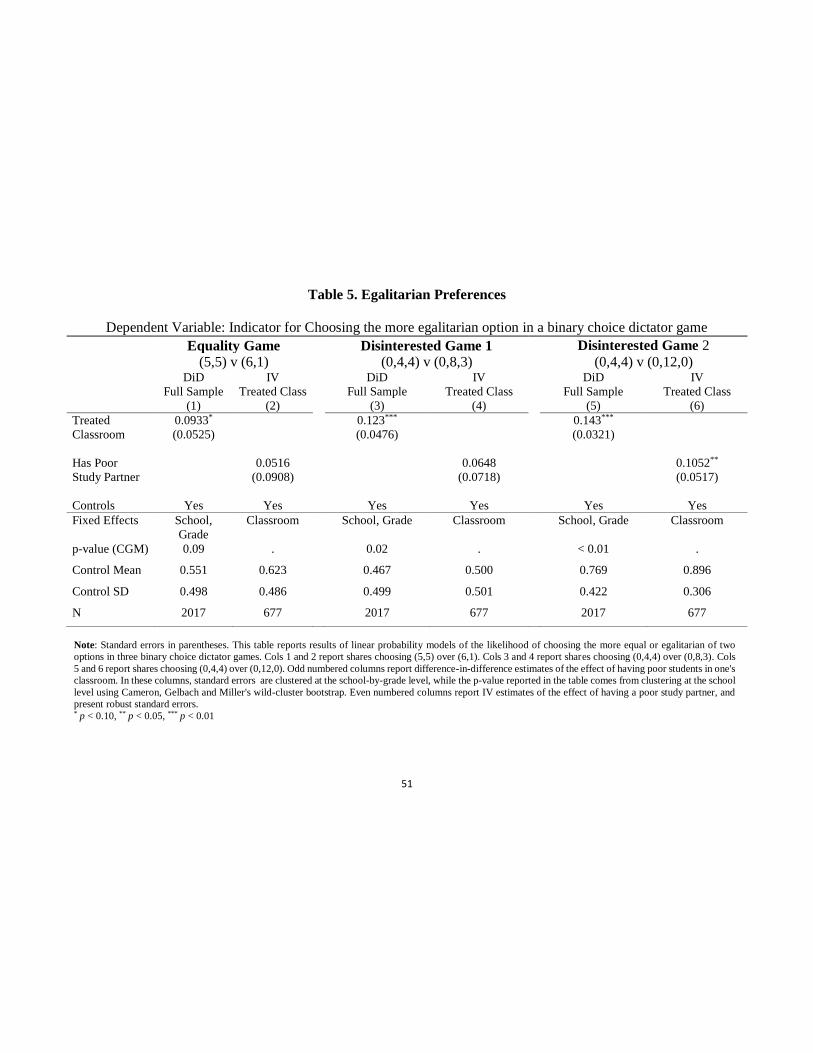
51

Table 5. Egalitarian Preferences

Dependent Variable: Indicator for Choosing the more egalitarian option in a binary choice dictator game

Equality Game Disinterested Game 1 Disinterested Game 2

(5,5) v (6,1) (0,4,4) v (0,8,3) (0,4,4) v (0,12,0) DiD

Full Sample

IV

Treated Class

DiD

Full Sample

IV

Treated Class

DiD

Full Sample

IV

Treated Class

(1) (2) (3) (4) (5) (6)

Treated

Classroom

0.0933*

(0.0525)

0.123***

(0.0476)

0.143***

(0.0321)

Has Poor

Study Partner

0.0516

(0.0908)

0.0648

(0.0718)

0.1052**

(0.0517)

Controls Yes Yes Yes Yes Yes Yes

Fixed Effects School,

Grade

Classroom School, Grade Classroom School, Grade Classroom

p-value (CGM) 0.09 . 0.02 . < 0.01 .

Control Mean 0.551 0.623 0.467 0.500 0.769 0.896

Control SD 0.498 0.486 0.499 0.501 0.422 0.306

N 2017 677 2017 677 2017 677

Note: Standard errors in parentheses. This table reports results of linear probability models of the likelihood of choosing the more equal or egalitarian of two

options in three binary choice dictator games. Cols 1 and 2 report shares choosing (5,5) over (6,1). Cols 3 and 4 report shares choosing (0,4,4) over (0,8,3). Cols

5 and 6 report shares choosing (0,4,4) over (0,12,0). Odd numbered columns report difference-in-difference estimates of the effect of having poor students in one's

classroom. In these columns, standard errors are clustered at the school-by-grade level, while the p-value reported in the table comes from clustering at the school

level using Cameron, Gelbach and Miller's wild-cluster bootstrap. Even numbered columns report IV estimates of the effect of having a poor study partner, and

present robust standard errors. * p < 0.10, ** p < 0.05, *** p < 0.01

52

Table 6. Discrimination Against Poor Children

Dependent Variable: Indicator for choosing lower-ability wealthy student over

higher-ability poor student (1) (2) (3) (4)

DiD-1

Full Sample

DiD-2

Full Sample

IV-1

Treated Class

IV-2

Full Sample

Treated Classroom -0.123**

(0.0466)

-0.256***

(0.0654)

Prize = Rs. 200 -0.110**

(0.0423)

-0.137**

(0.0540)

-0.0582

(0.0757)

-0.0415

(0.126)

Prize = Rs. 500 -0.250***

(0.0583)

-0.314***

(0.0498)

-0.126*

(0.0713)

-0.101

(0.135)

(Treated Classroom) x

(Prize = Rs. 200)

0.1153*

(0.0667)

(Treated Classroom) x

(Prize = Rs. 500)

0.186*

(0.0939)

Has Poor Study Partner

-0.147*

(0.0885)

-0.118

(0.156)

(Poor Study Partner) x

(Prize = Rs. 200)

-0.0337

(0.210)

(Poor Study Partner) x

(Prize = Rs. 500)

-0.0510

(0.227)

Fixed Effects School, Grade School, Grade Classroom Classroom

Control Mean 0.226 0.226 0.220 0.220

Control SD 0.419 0.419 0.418 0.418

N 342 342 116 116 Note: Standard errors in parentheses. This table reports results of linear probability models of the likelihood of

discriminating: i.e. choosing a wealthy teammate despite the poor child winning the first round race. Cols 1 and 2

report difference-in-difference estimates of the effect of having poor students in one's classroom, with robust standard

errors. Cols 3 and 4 report parallel IV estimates of the effect of having a poor study partner, with robust standard

errors. * p < 0.10, ** p < 0.05, *** p < 0.01

53

Table 7. Structural Estimates

Estimates Difference

-11*

(6.5)

-1

(2.8)

Boost in probability of winning from

choosing high ability teammate (δ)

Moments (Probability of Discriminating)

Empirical Predicted Empirical Predicted

Control Students:

Stakes = Rs. 50 35% 46% 4% 11%

Stakes = Rs. 200 27% 24% 3% 0%

Stakes = Rs. 500 5% 1% 2% 0%

Treated Students:

Stakes = Rs. 50 20% 32% 6% 16%

Stakes = Rs. 200 15% 18% 4% 1%

Stakes = Rs. 500 6% 0% 2% 0%

Mean distaste for poor teammate

relative to rich (µD), in Rupees

Std. Dev. of distaste for poor teammate

relative to rich (σD), in Rupees

Notes: Estimates from minimum-distance estimator using the moments shown, and weights given

by the inverse of each moment's variance. Standard errors are in parentheses.

Treated

26

(4.8)

Against Poor Against Rich

Control

37

(4.4)

6

(1.9)

5

(2.1)

0.08

(.1)

54

Table 8. Willingess to Play with Poor Children

Dependent Variable:

Willingness to Accept to Attend Play Date (Rupees) (1) (2) (3) (4)

Specification:

Sample:

DiD

Full Sample

DiD

Younger Sibs

IV

Treated Class

DiD+IV

Full Sample

Treated Classroom -6.961***

(1.075)

-6.262***

(1.698)

-1.891

(2.355)

Has Poor Study Partner

-7.878***

(2.889)

-7.226**

(3.272)

Controls Yes Yes Yes Yes

Fixed Effects School, Grade School, Grade Classroom School, Grade

p-value (CGM) < 0.01 0.02 . .

Control Mean 36.84 40.02 32.08 36.84

Control SD 11.94 13.67 14.75 11.94

N 2017 1143 677 2017

Note: Standard errors in parentheses. This table reports regression results for wealthy students' minimum

willingness to accept to attend a play date with poor children. Col 1 reports a difference-in-differences estimates

of the effect of having poor students in one's classroom, with standard errors clustered at the school-by-grade level.

The p-value reported in the table instead is calculated using clustering at the school level (k=14) using Cameron,

Gelbach and Miller's wild-cluster bootstrap. Col 2 reports the same specification as Col 1, but restricts the sample

to students who have older siblings enrolled in the same school. Col 3 reports IV estimates of the effect of having

a poor study partner, and presents robust standard errors. Col 4 reports a specification estimating both the

classroom level effect using the difference-in-differences term and an additional effect of having a poor study

partner, with standard errors clustered at the school-by-grade level. * p < 0.10, ** p < 0.05, *** p < 0.01

55

Table 9. Test Scores in English, Hindi and Math

Dependent Variable: Normalized Test Score

Combined English Hindi Math Specification:

Sample:

DiD

Full

IV

Treated

DiD

Full

IV

Treated

DiD

Full

IV

Treated

DiD

Full

IV

Treated

(1) (2) (3) (4) (5) (6) (7) (8)

Treated Classroom -0.024

(0.068)

-0.087*

(0.050)

0.0260

(0.0632)

0.037

(0.0466)

Has Poor Study

Partner

-0.025

(0.132)

-0.066

(0.135)

-0.181

(0.172)

0.0146

(0.083)

Controls Yes Yes Yes Yes Yes Yes Yes Yes

Fixed Effects School,

Grade

School,

Grade

Classroom School,

Grade

Classroom School,

Grade Classroom

p-value (CGM) 0.76 . 0.09 . 0.72 . 0.45 .

Control Mean 0 0.0466 0 0.0266 0 0.0372 0 0.0761

Control SD 0.594 0.628 1.000 1.127 1.000 1.021 1.000 0.974

N 2017 677 2017 677 2017 677 2017 677

Note: Standard errors in parentheses. This table reports effects on an index of test scores comprised of equally weighted normalized scores in English normalized

test scores of wealthy students in English (Cols 3 and 4), Hindi (Cols 5 and 6), (Cols 7 and 8). Odd numbered columns report difference-in-difference estimates

of the effect of having poor students in one's classroom. In these columns, standard errors are clustered at the school-by-grade level, while the p-value reported in

the table comes from clustering at the school level using Cameron, Gelbach and Miller's wild-cluster bootstrap. Even numbered columns report IV estimates of

the effect of having a poor study partner, and present robust standard errors. * p < 0.10, ** p < 0.05, *** p < 0.01

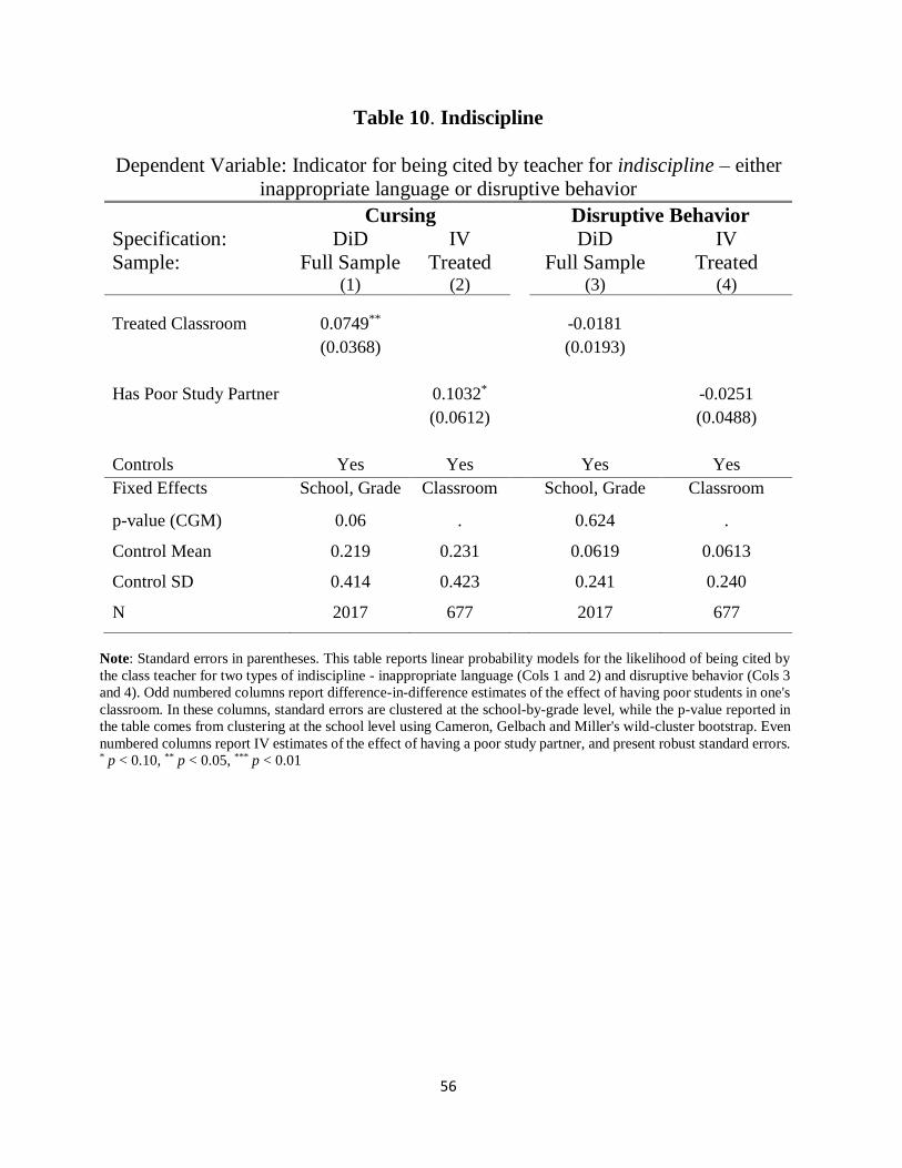
56

Table 10. Indiscipline

Dependent Variable: Indicator for being cited by teacher for indiscipline – either

inappropriate language or disruptive behavior

Cursing Disruptive Behavior

Specification:

Sample:

DiD

Full Sample

IV

Treated

DiD

Full Sample

IV

Treated (1) (2) (3) (4)

Treated Classroom 0.0749**

(0.0368)

-0.0181

(0.0193)

Has Poor Study Partner

0.1032*

(0.0612)

-0.0251

(0.0488)

Controls Yes Yes Yes Yes

Fixed Effects School, Grade Classroom School, Grade Classroom

p-value (CGM) 0.06 . 0.624 .

Control Mean 0.219 0.231 0.0619 0.0613

Control SD 0.414 0.423 0.241 0.240

N 2017 677 2017 677

Note: Standard errors in parentheses. This table reports linear probability models for the likelihood of being cited by

the class teacher for two types of indiscipline - inappropriate language (Cols 1 and 2) and disruptive behavior (Cols 3

and 4). Odd numbered columns report difference-in-difference estimates of the effect of having poor students in one's

classroom. In these columns, standard errors are clustered at the school-by-grade level, while the p-value reported in

the table comes from clustering at the school level using Cameron, Gelbach and Miller's wild-cluster bootstrap. Even

numbered columns report IV estimates of the effect of having a poor study partner, and present robust standard errors. * p < 0.10, ** p < 0.05, *** p < 0.01