Barcelona GSE Working Paper Series

Working Paper nº 815

Familiarity and Competition: The Case of Mutual Funds

Ariadna Dumitrescu Javier Gil-Bazo

March 2015

Familiarity and Competition:

The Case of Mutual Funds∗

Ariadna Dumitrescu

ESADE Business School and University Ramon Llull

Javier Gil-Bazo

University Pompeu Fabra and Barcelona GSE

First Version: March 2015

Abstract

We build a model of mutual fund competition in which a fraction of investors (“unsophisticated”)exhibit a preference for familiarity. Funds differ both in their quality and their visibility: Whileunsophisticated investors have varying degrees of familiarity with respect to more visible funds,they avoid low-visibility funds altogether. In equilibrium, bad low-visibility funds are drivenout of the market of sophisticated investors by good low-visibility funds. High-visibility fundsdo not engage in competition for sophisticated investors either, and choose instead, to cater tounsophisticated investors. If familiarity bias is high enough, bad funds survive competition fromhigher quality funds despite offering lower after-fee performance. Our model can thus shed lighton the persistence of underperforming funds. But it also delivers a completely new prediction:Persistent differences in performance should be observed among more visible funds but not inthe more competitive low-visibility segment of the market. Using data on US domestic equityfunds, we find strong evidence supporting this prediction. While performance differences surviveat least one year for the whole sample, they vanish within the year for low-visibility funds. Theseresults are not explained by differences in persistence due to fund size or investment category.The evidence also suggests that differences in persistence are not the consequence of other formsof segmentation on the basis of investor type (retail or institutional) or the distribution channel.

JEL codes: G2; G23.Keywords: familiarity bias; competition; mutual funds; performance persistence.

∗Corresponding author: Javier Gil-Bazo. Universitat Pompeu Fabra, c/Ramon Trias Fargas 25-27,08005 Barcelona, Spain. E-mail: javier.gil-bazo@upf.edu. Tel.: +34 93 542 2718. Fax: +34 93 5421746. Ariadna Dumitrescu acknowledges the financial support of Spain’s Ministry of Education (grantECO2011-24928), Government of Catalonia (grant 2014-SGR-1079) and Banc Sabadell. Javier Gil-Bazoacknowledges the financial support of the Government of Catalonia (grant 2014-SGR-549).

1 Introduction

Academics have spent decades teaching the benefits of portfolio diversification for risk-averse

investors. Despite this advice, investors tend to concentrate their holdings in stocks of companies

headquartered in their country of residence and within domestic firms, they choose those to which

they are geographically, linguistically or culturally close, and even the company they work for

(French and Poterba, 1991; Huberman, 2001; Grinblatt and Keloharju, 2001; Benartzi, 2001).

Familiarity bias can explain this lack of diversification. Familiarity biased investors overestimate

the risk of unfamiliar firms or underestimate their expected return, or both.1 Familiarity bias

does not only affect the composition of investors’ stock portfolios. Bailey et al. (2011) report

that many mutual fund investors exhibit a propensity to select funds with headquarters close

to where they live, and this bias has the strongest statistical and economic association with

poor fund choices among all other behavioral biases.2 While the impact of familiarity bias on

asset prices has been studied in the literature (e.g., Cao et al., 2009), its effects on the market

for financial services remains unexplored. In this paper we study how familiarity bias shapes

competition in the market for mutual funds, as well as the consequences for fund performance.

The main goal of our paper is to investigate whether familiarity bias can explain two closely

related puzzles documented in the mutual fund industry: fee setting and performance persis-

tence. There is abundant empirical evidence that differences in mutual fund fees do not reflect

differences in before-fee performance (see, e.g., Gil-Bazo and Ruiz-Verdu, 2009). There is also

much evidence that performance persists at least in the short run, and even in the long run

in the case of the worst performing funds (Carhart, 1997). Both pieces of evidence contradict

the central prediction of Berk and Green (2004). These authors assume that investors demand

shares of all funds with expected risk-adjusted performance net of fees and other costs higher

than their reservation return, which is assumed to be zero. In the presence of diseconomies of

scale, flows of money into (out of) funds decrease (increase) fund performance. In equilibrium,

1An alternative explanation is that investors possess and exploit non-public information about familiarinvestments (Ivkovic and Weisbenner, 2005, Massa and Simonov, 2006). However, individuals’ portfoliosof local holdings do not outperform passive benchmarks by a statistically or economically significantamount (Seasholes and Zhu, 2010).

2Bailey et al. (2011) find that investors that invest in funds headquartered in the proximity of theirplace of residence tend to invest in funds with higher expense ratios, higher front end loads, and higherturnover, after controlling for other behavioral biases.

2

all funds offer the same expected performance net of fees. Therefore, fees are higher for funds

with higher before-fee expected performance, and differences in net performance between funds

are unpredictable.

In order to achieve our goal, we build a model that captures three aspects of familiarity. First,

an investor’s familiarity with a mutual fund is defined by the distance between the investor and

the fund. One can think of distance as geographic distance but also, and more generally, as

being inversely related to the amount of exposure to information about the mutual fund due to

past investment experience with the same fund or management company, amount of personal

referrals, or other reasons. Second, some funds are more visible than others, making them more

familiar to all investors. The idea is that while some investors are more familiar with Fidelity

Investments and other investors are more familiar with Vanguard Group, most of them are more

familiar with both Fidelity and Vanguard funds than with those offered by small companies, such

as Merger Funds or Buffalo Funds. Third, not all investors are equally prone to familiarity bias.

More financially sophisticated investors overcome lack of familiarity by investing in research and

comparing funds, either because they have more at stake–they are wealthier–or because learning

is less costly for them–they are more financially literate, more experienced, or better educated.3

We study a market in which actively managed funds of two different qualities compete to at-

tract investors’ money. In this market there are two types of investors: unsophisticated investors,

prone to familiarity bias; and sophisticated investors. In addition to quality, funds differ in their

visibility. While unsophisticated investors suffer a disutility from investing in highly visible but

less familiar funds, their lack of familiarity with low-visibility funds is so high that they shun

them altogether.4 Our model delivers a number of predictions. First, in equilibrium bad low-

visibility funds are driven out of the market by good low-visibility funds. Second, in equilibrium

there is segmentation in that high-visibility funds cater to unsophisticated investors and refuse

to compete for sophisticated investors, who invest only in good low-visibility funds. Third, if

the disutility of investing in unfamiliar funds is high enough relative to performance differences,

3Bekaert et al. (2014) study the international diversification of 3 million 401(k) accounts and reportthat investor income, wealth, education, and financially literacy are all strongly and positively associatedwith international diversification.

4One may think of the disutility from investing in unfamiliar funds as the decrease in investor’sperception of risk-adjusted performance for such funds.

3

bad high-visibility funds coexist with good high-visibility funds in the unsophisticated segment

of the market and offer lower after-fee expected performance. Therefore, familiarity bias can

explain the puzzling survival of funds that are expected to underperform. But the model also

delivers a completely new prediction: While we can expect differences in after-fee performance

among high-visibility funds, we should expect no differences in after-fee performance among

low-visibility funds. This is a natural consequence of segmentation: Competition is fierce in

the low-visibility segment of the market, but is relaxed by familiarity bias in the high-visibility

segment. To the extent that quality persists, the model predicts that observed differences in per-

formance among the more visible funds also persist through time. In contrast, any performance

differences among low visibility funds are the consequence of luck and short-lived. Finally, for

intermediate levels of familiarity bias, the model yields a new prediction regarding strategic fee

setting: High-visibility funds charge higher fees on average than low-visibility funds.

To test the model’s predictions, we use US domestic equity mutual fund data covering the

1993-2010 period. We proxy for fund visibility using the size, age and diversity of investment

categories of the fund’s family. We also use advertising expenditures at the family level. Mea-

suring both past and future performance using the four-factor model of Carhart (1997), we find

strong evidence of persistent performance differences across funds over a one-year period, con-

ditional on other observable fund characteristics. In contrast and consistently with the model’s

prediction, the least visible funds exhibit no persistence in performance. This is true for both

underperformance and outperformance. Funds whose past performance has been in the bottom

decile of the distribution in the last twelve months and which belong to the group of low-visibility

funds, do not perform significantly worse than funds with median past performance. Similarly,

the performance of less visible recent winners is not significantly better than that of the median

fund. These results are not driven by different performance persistence for funds of different

sizes or funds in different investment categories.

When past performance is measured using raw returns, we only find evidence of performance

differences between the worst recent performers and the median fund for the whole sample.

Again, low-visibility funds exhibit no evidence of performance persistence.

We consider and test two alternative explanations. First, while some mutual fund shares are

4

available to retail investors, others can be purchased only by institutional investors. Regardless

of the economic reasons why this form of product differentiation arises in the mutual fund mar-

ket, one would expect institutional investors to be more sophisticated than retail investors, and

thus, more responsive to differences in performance. Second, there exists evidence of large dif-

ferences between funds sold directly to investors and funds sold through brokers. In particular,

funds in the broker channel tend to be more expensive and underperform, even before expenses

(Bergstresser et al., 2009; Christoffersen et al., 2013; Del Guercio and Reuter; 2014). As ex-

plained below, such segmentation may arise as the consequence of differences in fee sensitivity

across investors, with the least fee-sensitive investors choosing to pay a mark-up for advice. To

rule out the possibility that our results are simply capturing differences between retail funds

and institutional funds or differences in persistence due to the distribution channel, we run a

subsample analysis of persistence. Results suggest that both retail funds and institutional funds

exhibit very similar levels of persistence. We do not find differences in performance persistence

between directly sold and brokered funds, either.

Finally, consistently with the model prediction and intermediate levels of familiarity bias,

we find that investors in low-visibility funds pay economically and statistically lower fees than

investors in all other funds.

Our paper is part of a literature that tries to understand why performance differences across

mutual funds persist. One possible explanation is that contrary to the assumption of Berk

and Green (2004), there are no diseconomies of scale in money management. Ferreira et al.

(2013) study the relationship between fund size and performance in 27 countries and find that

most countries do not have decreasing returns to scale in asset management. However, they

also document that performance persists even in those countries with decreasing returns to

scale. Similarly, Bessler et al. (2010) show that outflows from underperforming funds alone

cannot eliminate their performance disadvantage. They do find, however, that outflows from

underperforming funds combined with manager replacement can cause reversals in performance.

Reuter and Zitzewitz (2010) study the effect of fund flows on performance using a regression

discontinuity approach and estimate diseconomies of scale of a magnitude larger than estimated

in standard regression but insufficient to eliminate performance persistence.

5

Therefore, empirical tests of the Berk and Green (2004) model suggest that fund flows do

not eliminate performance differences. But, what stops money from flowing freely from under-

performing to outperforming funds? Berk and Tonks (2007) and Glode et al. (2011) provide an

answer to that question. Berk and Tonks (2007) argue that differences in the speed of learning

across investors cause the composition of a fund’s investor base to change with performance,

since the first investors to leave or enter a fund are those who update their beliefs the fastest.

As a consequence, remaining investors of a fund that has underperformed in the past have a

lower flow-to-performance sensitivity, which prevents the fund’s assets from shrinking should

the fund continue to underperform in the future. They report evidence that funds that have

performed poorly in each of the last two years are more likely to underperform in the future

than funds that have performed poorly only in the last year. Glode et al. (2011) study time

variation in performance persistence and find evidence that mutual fund performance persistence

is strongest following periods of high market returns and vanishes after periods of low market

returns. The authors argue that differences in performance persistence across market conditions

may be explained by time-varying differences in the participation of unsophisticated investors

in the mutual fund market, with a higher fraction of unsophisticated investors leading to larger

deviation from the no-predictability equilibrium. Like Berk and Tonks (2007) and Glode et al.

(2011), we also propose lack of investor sophistication as the reason why fund performance per-

sists. Unlike those papers, we try to unveil the specific bias that makes unsophisticated investors

less sensitive to differences in performance in the first place. We also provide an explanation for

why competition for sophisticated investors is not sufficient to equate performance across funds.

A challenge of any model of mutual fund competition is to explain why low-quality funds

are not priced out of the market by high-quality funds in the absence of diseconomies of scale.

In a duopoly model of vertical differentiation, Metrick and Zeckhauser (1998) show that when

investors have different subjective valuations of fund quality, the high-quality fund will sell at a

higher price to the most quality-sensitive investors, while the bad-quality fund will survive by

selling at a low price to less quality-sensitive investors. Moreover, if a fraction of all investors

are uncertain about fund quality, it is possible to have a pooling equilibrium in which low-

quality funds set the same price as high-quality funds and sell only to uninformed investors.

6

Nanda et al. (2000) study a model in which mutual fund managers compete to attract investors

with low liquidity needs by offering them lower management fees and imposing exit fees. In

equilibrium, more skilled fund managers outbid less skilled managers, who become liquidity

providers. Gil-Bazo and Ruiz-Verdu (2008) study a market with multiple mutual funds and

identical investors in which a fund manager’s ability is known only by the manager herself. In

this setup, only pooling equilibria are possible. However, under the assumption that a fraction

of investors are not responsive to the information contained in mutual fund fees, the authors

show the existence of a separating equilibrium in which high-quality funds signal their quality

through low fees and low-quality funds must cater to price-inelastic investors to whom they

charge high fees. Gennaioli et al. (2015) model a duopoly market in which investors wish to

invest in risky assets only through a trusted money manager. Half of the investors trust one fund

more than the other, who, in turn, is trusted more by the other half. More trust in the manager

reduces investor’s disutility from taking risk. In equilibrium managers split the market with each

investor delegating his portfolio to his most trusted manager. Equilibrium fees are proportional

to expected returns, which provides managers with incentives to direct their investors towards

assets with higher perceived expected returns.

Like the models cited above, ours departs from the perfectly competitive equilibrium and

explains why strategically-set fees may not offset differences in quality. The novelty of our

model is that we introduce a new dimension along which mutual funds differ: familiarity to

investors. Moreover, by allowing for an extreme level of familiarity that depends only on the

characteristics of funds but not on those of investors, low visibility, we can empirically distinguish

between our model and other models that generate persistent differences in fund performance

using the available mutual fund data. In this sense, our model is more closely related to the

work of Sun (2014), who studies a market in which segmentation between directly sold funds

and brokered funds, which are bundled with advice, arises as the consequence of differences in

investors’ fee sensitivity.

The results of our paper have important implications. First, the empirical results combined

with our theory suggest that the presence of familiarity biased investors in the mutual fund

market, far from being negligible, is large enough to generate persistent differences in fund

7

performance. With over USD15 trillion of US investors’ money invested in mutual funds at year-

end 2013, USD6.5 trillion of which are held through defined contribution plans and individual

retirement accounts, the consequences of persistent differences in performance for investor wealth

are considerable.5 Our results suggest that such differences would be attenuated by reducing

investors’ familiarity bias. Second, the presence of sophisticated investors in the market is not a

sufficiently strong incentive for funds to set fees that offset differences in before-fee performance.

Third, entry of new competitors is not likely to alleviate this situation in the short term due to

lack of familiarity of investors with new fund families.

The rest of the paper is organized as follows. In section 2, we present the theoretical frame-

work of our analysis. In section 3, we describe the data set. In section 4 we present our main

empirical results. Section 5 explores two alternative hypotheses. Section 6 investigates differ-

ences in fees. Finally, section 7 concludes. All proofs can be found in the Appendix.

2 The model

Actively managed funds compete for investors’ money. We consider two continuums of investors:

sophisticated investors, with density λS ; and unsophisticated investors, with density λU . Unso-

phisticated investors are prone to familiarity bias: they derive a disutility from investing in less

familiar funds. As an alternative to active funds, investors can choose to invest with an index

fund offering a zero expected risk-adjusted return and charging a zero fee. Active funds differ

from each other in two dimensions: quality and visibility. More specificallly, we assume that

there are four active funds and each one of the four funds is different from the other three in

terms of either quality (θ) or visibility (v), or both, with θ ∈ {G,B} and v ∈ {H,L}, where G

and B denote high and low quality, respectively, and H and L denote high and low visibility,

respectively. A fund’s type is common knowledge. We denote the expected risk-adjusted per-

formance of high-quality (henceforth good) and low-quality (henceforth bad) funds by RG and

RB, respectively, with RG > RB. For simplicity, we refer to expected risk-adjusted performance

as return. When choosing among high-visibility funds, investors exhibit a preference for more

5Data from the Investment Company Institute’s 2014 Investment Company Fact Book,http://www.icifactbook.org.

8

familiar funds. However, the disutility of investing in low-visibility funds to unsophisticated

investors is so large that no unsophisticated investor ever finds it optimal to invest in them.

This means that unsophisticated investors choosing to invest in active funds are restricted to

the two high-visibility funds.

To model unsophisticated investors’ preference for more familiar funds, we build on Hotelling’s

(1929) model of horizontal differentiation. Unsophisticated investors are uniformly distributed

along a familiarity line of length λU and the two high-visibility funds are located at the extremes

of the line. The good, high-visibility fund is located at x = 0. The bad, high-visibility fund

is located at x = λU . We assume that the disutility of investing in a less familiar fund is a

quadratic function of the distance between the investor and the fund.6 In particular, an investor

living at x suffers a disutility kx2 from investing in the good fund and a disutility of k (λU − x)2

from investing in the bad fund.

2.1 The investor’s problem

Each investor is endowed with one dollar, and pays a fee, f, for investing with an active mutual

fund. Sophisticated investors derive a utility equal to USθv = Rθ − fθv, for investing in the active

mutual fund of quality θ and visibility v. The unsophisticated investor i derives a utility equal

to UUi,θv = Rθ − fθv − kd2i,θv, where di,θv denotes the distance between the investor and the fund.

Utility from investing with the index fund is zero. An investor decides to invest with fund θv

as long as the utility from investing with that fund is both positive and higher than the utility

from investing with any other active fund.

The demand of the sophisticated investors is split equally across all active funds offering the

highest positive net-of-fee return and is zero for all the other funds.

The demand of the unshophisticated investors for the low-visibility funds is zero by assump-

tion. Each unsophisticated investor chooses to invest in the high-visibility fund offering the

highest utility given the fund’s return, fee, and the distance between the fund and the investor,

as long as this utility is positive, otherwise she invests in the index fund. In case that both funds

offer the same positive utility, her wealth is split equally between them.

6Our results are qualitatively the same if we assume a linear function for disutility.

9

2.2 The manager’s problem

Fund managers choose the fees that maximize their profits given investors’ demand functions

and the other managers’ strategies. Without loss of generality, we assume that the marginal

cost to the manager of operating the fund is zero. Therefore, the manager’s problem becomes:

maxfθv

Πθv = fθv (qU,θv + qS,θv) ,

where qU,θv, qS,θv denote the total demand for the fund from unsophisticated and sophisticated

investors, respectively.

2.3 Equilibrium

The two high-visibility funds, GH and BH, are differentiated products for unsophisticated

investors because of their location. The two low-visibility funds, GL and BL, on the other

hand, are not differentiated in that they are perfect substitutes in the sophisticated investors’

utility function: All sophisticated investors value net returns equally and invest in the fund that

gives them the highest net return. The low-visibility funds engage in Bertrand-like competition.

Since the returns are such that RG > RB, the GL fund can drive the BL fund out of the market

simply by undercutting the fee. The BL fund cannot set a fee, fBL, lower than zero. By setting

a fee such that fGL < RG− RB ≡ ∆, the GL fund gains all the market of sophisticated investors

and the BL fund does not operate in the market.

Lemma 1 In equilibrium, no investors choose to invest in the bad low-visibility (BL) fund.

In next lemma, we show that sophisticated investors do not invest in high-visibility funds,

either.

Lemma 2 In equilibrium, high-visibility funds cater to unsophisticated investors and low-visibility

funds cater to sophisticated investors.

To see how this form of segmentation arises in equilibrium, assume that high-visibility funds

decide to compete against low-visibility funds for sophisticated investors. For the same reasons

10

that BL is driven out of the market, BH does not attract any sophisticated investors. If the two

good funds, GH and GL, engage in price competition, since both funds offer the same return

RG, each has an incentive to undercut its fee until the fee equals zero, i.e., fGL = fGH = 0. At

that fee, both GH and GL make zero profits. However, GH can always charge an arbitrarily

small but positive fee and make positive profits by operating only with unsophisticated investors.

More specifically, it is sufficient for the GH fund to charge a fee lower than ∆ ≡ RG− RB to

dominate the BH fund for investors sufficiently familiar with GH regardless of the fee charged

by the BH fund. This ensures that those investors that are closest to GH are willing to invest

in it, and therefore the GH makes a positive profit.

The two high-visibility funds, GH and BH, compete only against each other for unsophis-

ticated investors. When all unsophisticated investors purchase low-visibility funds, the market

is covered. When some unsophisticated investors decide to invest in the index fund, the mar-

ket is not covered and the two highly visible funds act as local monopolies. Depending on the

model parameters, we have three possible situations. First, the market is covered and all un-

sophisticated investors invest in the GH fund. This happens when the disutility of investing in

unfamiliar funds, which depends on k, is small relative to the difference in returns, ∆, and given

the distance between both funds λU . Second, the market is covered and the two high-visibility

funds share the market of unsophisticated investors. This happens for an intermediate value of

k, given the other parameters. Third, when k is very high, the market is not covered: Funds act

as local monopolies and set fees accordingly. Consequently, familiarity bias allows both good

and bad funds to coexist in equilibrium as long as differential performance is not very large

relative to the utility cost of investing in unfamiliar funds. These results are presented in the

following Proposition:

11

Proposition 1 In equilibrium, the fees charged by the funds are the following

f∗GH =

∆− k (λU )

2 if k ≤ k0,

k (λU )2 + 1

3∆ if k0 < k < k1,

23RG if k ≥ k1,

,

f∗BH =

0 if k ≤ k0,

k (λU )2 − 1

3∆ if k0 < k < k1,

23RB if k ≥ k1.

,

f∗GL =

λU

λS+λU

(∆− kλ2

U

)− ε if k ≤ k0,

min {∆, f∗} − ε if k ∈ (k0, k1)

min {∆, f∗∗} − ε if k ≥ k1

,

f∗BL = 0,

and the quantities invested in each fund are

q∗S,GL = λS ,

q∗S,GH = q

∗S,BH = q

∗S,BL = 0,

q∗U,GL = q

∗U,BL = 0,

q∗U,GH =

λU if k ≤ k0,

12kλU

(k (λU )

2 + 13∆)

if k0 < k < k1,√RG3k if k ≥ k1,

,

q∗U,BH =

0 if k ≤ k0,

12kλU

(k (λU )

2 − 13∆)

if k0 < k < k1,√RB3k if k ≥ k1.

,

where ε is strictly positive and arbitrarily small, and the definitions of f∗, f∗∗, k0 and k1 are

provided in the Appendix.

In the cases in which the BH fund survives, i.e., when k > k0, it charges a lower fee than the

GH fund. However, the difference in fees between both funds equals2

3∆, which is not enough

12

to fully offset the difference in before-fee performance, ∆. Therefore, when the bad visible fund

survives in the market, it does so despite offering lower net performance than the good visible

fund. In other words, in equilibrium, investors expect differences in performance between highly

visible funds. Notice that our model is static. However, since there is no asymmetric information

and therefore, no role for learning about performance, a dynamic model built as a succession

of static models would yield an identical outcome provided that pre-fee performance does not

change over time. This observation helps understand why differences in net performance can

persist.

Although we have characterized three different cases, we believe that the case in which only

the GH fund serves unsophisticated investors is not empirically plausible, as it would imply that

there are no differences in before-fee performance between actively managed funds. Therefore,

in next section, we rule out the first case and test the model’s prediction for the other two cases:

Persistent differences in performance should be observed among high-visibility funds but not

among low-visibility funds, as Bertrand-like competition in the latter segment of the market

ensures homogeneity in quality and fees.

In order to ensure that the GH fund does not want to deviate from the equilibrium with

segmentation, the GL fund sets a lower fee than that charged by GH so that the profit ob-

tained by GH from serving only unsophisticated investors is higher than the profit obtained by

lowering the fee in order to serve also the entire market of sophisticated investors. Further, for

intermediate values of k, i.e., when k0 < k < k1, the fee charged by GL is lower than the average

fee charged by high-visibility funds. This relationship is contained in the following corollary:

Corollary 1 In equilibrium, for k0 < k < k1, the average fee of high-visibility funds is higher

than the fee of the low-visibility fund1

2(fGH + fBH) > fGL.

Although we test for differences in fees in Section 6, since this is not an unambiguous

prediction of the model, most of of our empirical analysis focuses on testing for differences in

persistence between high- and low-visibility funds.

13

3 Data

Our main source of data is the CRSP Survivor-Bias-Free US Mutual Fund Database. Since

some of the variables employed in the analysis are available only since the early 1990s, we

restrict our attention to the 1993-2010 period. We exclude index, non-domestic, non-diversified,

and non-equity funds.7 We aggregate monthly data for different share classes at the fund level.

In particular, we compute fund total net assets as the sum of assets of all share classes of

the same portfolio, fund age as the number of years since inception of the oldest class, and all

other variables (return, expense ratio, 12b-1 fee, front-end and back-end loads) as asset-weighted

averages of those variables at the class level. We also compute family age and family assets as the

age of the oldest fund in the family and the sum of assets of all funds in the family, respectively.

Funds and families are identified using CRSP’s crsp portno and mgmt cd variables, respectively.

When those variables are not available, we use fund name and management company name,

instead. To mitigate the effect of documented biases in the CRSP database, we exclude all

fund-month observations with total net assets below $15 million and age less than three years

(Elton et al., 2011; Evans, 2010). Also, we winsorize expense ratios, 12b-1 fees, and turnover at

1% of each tail each month before aggregating class data at the portfolio level.

Throughout the paper, we evaluate mutual fund performance using Carhart’s (1997) four-

factor model:

rit = αi + βrmrf,irmrft + βsmb,ismbt + βhml,ihmlt + βpr1y,ipr1yt + εit, (1)

where rit is fund i’s return in month t in excess of the 30-day risk-free interest rate, as proxied

by Ibbotson’s one-month Treasury bill rate, and rmrft, smbt and hmlt denote the return on

portfolios that proxy for the market, size, and book-to-market risk factors, respectively. The

term pr1yt is the return difference between stocks with high and low returns in the previous

7To identify US domestic equity funds, we use the information in CRSP on investment categoryas follows. For years in which the only objective code available is Wiesenberger’s (wbrger obj cd), weconsider as US domestic equity those funds with the codes: G; G-I; I-G; MCG; GCI; LTG; MCG; SCG;and IEQ. For years 1993-1999, we use the si obj cd codes: AGG; GMC; GRI; GRO; ING; SCG. Foryears 2000-2010, we use the lipper class name codes: LCVE; MLVE; EI; EIEI; LCCE; MLCE; LCGE;MLGE; MCVE; MCCE; MCGE; SCVE; SCCE; and SCGE. Index funds are identified by the CRSP’sindex fund flag variable when available and by portfolio name otherwise.

14

year and is included to account for passive momentum strategies. We obtain the time series of

interest rates, the Fama-French factors, and momentum from Kenneth French’s website.

To estimate fund i’s risk-adjusted performance in month t, we first regress the fund’s excess

return on the three Fama-French factors and momentum over the previous three years. If less

than 36 monthly observations of previous data are available, we require at least 30 observations.

We then compute an estimate of fund i’s alpha in month t, αit, as the difference between the

fund’s excess return in month t and the dot product of the vectors of estimated betas and factor

realizations in that month.

We are interested in testing whether past performance predicts future performance over

multi-period horizons. To compute risk-adjusted performance over the prior h months in month

t, which we denote by αi,t−h:t−1, we sum monthly estimated alphas from months t−h to month

t− 1. Future performance, denoted by αi,t:t+m, is computed as the sum of monthly alphas from

months t to month t +m. Throughout the paper, we will focus on annual performance, so we

set h = 12 and m = 11.

We compute flows of money to mutual funds from monthly data on assets under management

and returns. In particular, monthly dollar flows in month t are computed as TNAt−TNAt−1(1+

rt), where TNA and r denote the fund’s total net assets and net return, respectively. Once we

have computed monthly dollar flows, we compute annual flows by adding dollar flows over the

year. In our regressions, we use annual relative flows defined as total annual flows divided by

total net assets at the end of the previous year. Relative flows are also winsorized at 1% of each

tail.

The final dataset contains information on an average number of 1,251 funds and 327 fund

families per month. Panels A and B of Table 1 contain summary statistics of fund characteristics

and performance for the 1993-2000 and 2001-2010 sample periods, respectively.

We use the following proxies for fund visibility:

1. Number of different investment categories in which the family offers mutual funds;

2. Family size, defined as total family assets;

3. Family age, computed as the age of the oldest fund in the family.

15

These variables have been previously proposed by Huang et al. (2007) as proxies for investor

participation costs. Low values of these variables characterize less visible funds.

For each one of these proxies, we create two dummy variables, denoted by LO and HI, which

equal one if fund i belongs to the bottom and top quartiles of the variable’s distribution in the

month prior to the evaluation period, respectively.

In addition to the three variables on fund visibility described above, we also use advertising as

a proxy for visibility. More specifically, we obtain data on advertising expenditures at the family

level from Kantar Media, which tracks advertising activity in a large variety of media including

magazines, newspapers, television, internet, and radio. We are able to collect information on

family advertising for about 18% of all fund-month observations in the 1995-2009 period. For

each family and month, we compute the average advertising expenditure over the previous 12

months. For this variable, we define the HI subsample as that containing funds in the top

quartile of the month’s distribution. It should be noted, however, that this subsample only

has 822 fund-month observations, so results for this subsample should be taken with caution.

Importantly, we set LO equal to one if the fund’s family is not contained in the advertising

database for that month.

Table 2 compares funds in the LO and HI subsamples on the basis of selected fund charac-

teristics. Less visible funds according to the number of investment categories, family size and

family age, are substantially smaller; they charge lower front-end loads, 12b-1 fees, and back-end

loads, but higher management fees; and they exhibit better risk-adjusted performance although

the difference in performance is not statistically significant. When we use family advertising to

proxy for fund visibility, we still find that funds in the LO subsample are smaller and charge

higher management fees. However, these funds also charge higher back-end loads and exhibit

worse performance.

16

4 Fund visibility and performance persistence

4.1 Methodology

To estimate persistence in mutual fund performance, the literature has employed two main alter-

native methodologies. The more traditional approach consists of sorting funds at the beginning

of each evaluation period on the basis of their past performance. Funds are then grouped in

quantile portfolios and portfolio returns are computed over the evaluation period. Finally, risk-

adjusted performance is measured using the time series of quantile portfolio returns. Failure to

find differences in risk-adjusted performance across portfolios is interpreted as lack of persistence

in mutual fund performance. This approach has been employed to study performance persis-

tence by Hendricks et al. (1993), Gruber (1996) and Carhart (1997), and Elton et al. (2011),

among others. The portfolio-based approach serves two purposes: It tests for persistence in

performance and it quantifies the value of investing on the basis of past performance. However,

the approach suffers from the same problem as all nonparametric methods, i.e., it requires a

large amount of data in multivariate settings.8

As an alternative, the regression-based approach consists of regressing future performance

on past performance and then testing whether the regression coefficient is zero. This approach

has been used by Busse et al. (2010), Elton et al. (2011), and Ferreira et al. (2013). By

imposing a parametric specification on the functional relation between future performance and

past performance and other variables, we can control for the effect of fund characteristics on

performance and allow for persistence to vary with those characteristics with less stringent

data requirements. Because we are interested in testing whether the degree of performance

persistence changes with fund visibility while controlling for a number of other variables, we

choose the regression approach.

We start by regressing future performance on past performance. Then, we allow for possible

8Suppose we wished to test for performance persistence while controlling for the effect of fund sizeon future performance. We could sort funds on both past performance and size, allocate funds to theresulting performance-size bins, and then compare portfolios that are neutral to size but correspond todifferent quantiles of past performance. Also, if our goal were to test whether performance persistencechanges with size, we could compare portfolios across both past performance and size bins. The problemis that the number of bins grows geometrically with the number of fund characteristics whose associationwith performance we wish to study.

17

non-linearities and regress future performance on dummy variables corresponding to different

deciles of past performance.

4.2 Results

To evaluate the prevalence of performance persistence in the entire sample, we estimate by

pooled OLS the regression equation:

αi,t:t+11 = δ0,t + δ1αi,t−12:t−1 +∆X ′i,t−1 + ξi,t:t+11, (2)

where each observation corresponds to one fund-month pair, X is a row vector of control vari-

ables, and ε denotes a generic error term. Control variables include: fund size in month t − 1,

defined as the natural logarithm of the fund’s assets; relative flows of money into the fund dur-

ing the year ending in month t − 1; fund age, defined as the natural logarithm of the fund’s

age in months; family size in month t− 1, defined as the natural logarithm of the assets under

management of the management company to which the fund belongs; and family age, defined

as the natural logarithm of the management company’s age in months. We also control for the

fund’s maximum front-end load, maximum back-end load, expense-ratio, and turnover ratio.

Since values of fees and turnover are reported for the entire fiscal year, their value in month t−1

is not strictly lagged with respect to future performance unless month t − 1 is the last month

of the fiscal year. To ensure that those variables are known before month t, we use a lag of 12

months for them. Like in the rest of the regressions presented in this paper, we allow for time

fixed effects and compute standard errors clustered by both fund and time to account for serial

and cross-sectional correlation of residuals, respectively.

The first column in Table 3 reports estimation results for equation (2). The coefficient on

past performance is positive and statistically significant at the 1% level, which suggests that

past performance persists for periods of at least one year, consistently with previous studies.

Both fund size and lagged flows are negatively and significantly associated with performance.

Funds belonging to larger management companies are associated with better performance, as

documented by Chen et al. (2004). Finally, the fund’s back-end load, expense ratio, and turnover

18

ratio are negatively related to performance, although the coefficient for turnover ratio is only

marginally statistically significant. In sum, these results are consistent with a large body of

empirical evidence that future US equity fund performance is predictable from the cross-section

of past performance and other fund characteristics.

We then interact the dummy variables LO and HI obtained according to the four proxies

of fund visibility with past performance, and estimate the regression equation:

αi,t:t+11 = θ0,t + θ1αi,t−12:t−1 + θ2αi,t−12:t−1LOi,t−1 + θ3αi,t−12:t−1HIi,t−1 +

+θ4LOi,t−1 + θ5HIi,t−1 +ΘX ′i,t−1 + υi,t:t+11, (3)

where we also include the two dummy variables to allow for the possibility of different means for

each group of funds. We are mainly interested in the coefficients θ2 and θ3. Columns 2-5 of Table

3 show the estimation results for each of the four proxies. The coefficients of the interaction of

performance with the LO dummy (θ2) are negative in all four cases and statistically significant at

the 1% level (family age), 5% level (number of investment categories and family advertising), and

10% level (family size). Estimation results, therefore, suggest that differences in performance

are shorter-lived for the least visible funds than for the rest of funds. Moreover, in contrast to

other funds, the least visible funds exhibit no performance persistence: The regression coefficient

on past performance for these funds, θ1+ θ2, is not statistically significant for any of the proxies

(unreported). We do not find differences in performance persistence between highly visible funds

and the rest of funds, which suggests that the relation between visibility and persistence is not

linear.

An obvious concern about these results is the possibility that they capture differences in

persistence across funds due to other fund characteristics. As mentioned in the introduction,

Elton et al. (2011) test the hypothesis that there should be less performance persistence among

larger funds, for which diseconomies of scale are more likely to be important, although they do

not find support for that hypothesis. Also, funds in different investment categories may exhibit

different degrees of performance persistence due to differences in the nature of the markets in

which they operate. To control for both possibilities, we include interactions of performance

19

with fund size and with dummies for investment categories. The estimation results are reported

in Table 4. The coefficients on the interactions of size with performance are negative, but not

statistically significant except in column 3 (Family Size), where it is only marginally significant.

The fact that the interaction of performance with size is not significant provides further support

to the finding of Elton et al. (2011) that performance persistence does not decline with fund size.

Further, all signs for the interactions of past performance with the LO dummies are negative

and the coefficients are statistically significant at the 1% level in all cases except for the family

advertising proxy (5%).

In sum, the results of Table 3 and 4 are strongly indicative that there exist differences in

performance persistence associated with fund visibility and that such differences in persistence

cannot be explained by differences in fund size or differences in investment categories.

Low persistence among certain types of funds may be the consequence of either recent under-

performers improving their performance or recent outperformers delivering lower performance,

or both. To disentangle the reason why less visible funds exhibit less persistent differences in

performance, we estimate the regression equation:

αi,t:t+11 = δ0,t +∑n

δ1,ndec ni,t−1

+∑n

δ2,ndec ni,t−1LOi,t−1 +∑n

δ3,ndec ni,t−1HIi,t−1

+δ4LOi,t−1 + δ5HIi,t−1 +∆X ′i,t−1 + νi,t:t+11, (4)

where dec ni,t−1 is a dummy variable that equals one if fund i’s performance is in the n-th decile

of all funds’ alphas over the prior twelve months. We omit the dummy variables corresponding to

the four central performance deciles, i.e., we only include in the regression the dummy variables

corresponding to the top three and bottom three performance deciles.

Once equation (4) has been estimated, we test whether the underperformance of funds

in the LO subsample is shorter-lived than that of otherwise similar recent underperformers.

More specifically, δ1,1 + δ2,1 captures the difference in expected performance between a LO-

fund whose past performance belongs to the first decile of the distribution and an otherwise

identical LO-fund with past performance in the central deciles. The coefficient δ1,1 captures the

20

difference in expected performance between a fund outside the LO and HI subsamples whose

past performance belongs to the first decile of the distribution and an otherwise identical fund

with performance in the central deciles. Therefore, a positive value of δ2,1 implies that the

performance of underperforming LO-funds converges faster to the median fund’s performance

than the performance of funds that do not belong to the LO or HI subsamples. Analogously, a

negative value of δ2,10 indicates that the performance of outperperforming LO-funds converges

faster to the median fund’s performance than the performance of funds that do not belong to

the LO or HI subsamples. Similarly, δ3,1 (δ3,10) is positive (negative) if HI-funds in the bottom

(top) performance decile converges to that of the median fund faster than that of funds with

LO = HI = 0.

Column 1 of Table 5 reports estimation results when no interactions with LO and HI

are included in the regression equation. The estimated coefficients on the three bottom (top)

performance decile dummies are negative (positive) and statistically significant at any signifi-

cance level. Future performance also appears to increase monotonically with past performance.

Differences in performance across deciles are economically significant: Recent top performers

outperform otherwise identical funds in the bottom decile by 180 basis points per year.

In columns 2-4 we report estimation results when interactions with LO and HI are included

and investor sophistication is determined according to the number of investment categories in

which the family offers funds, family size, and family age. The coefficient on the interaction

between the bottom decile dummy and LO, δ2,1, is positive and statistically significant, suggest-

ing that low-visibility underperforming funds exhibit better relative performance than otherwise

similar underperforming funds. In contrast, none of the coefficients on the interaction of the

bottom decile dummy and HI is statistically significant. When we use family advertising to de-

fine fund visibility, we find no difference in performance persistence for underperforming funds

in the low-visibility subsamples and otherwise similar funds. As mentioned above, when the

fund’s family is not contained in the advertising database for that month, we assume that the

advertising expenditures are zero for that family and set LO equal to one. This approach may

overestimate the number of funds in the low-visibility subsample.

We then ask whether good performance reverts faster for low-visibility funds. The answer is

21

yes: The coefficients on the interaction terms between LO and the top decile dummy, δ2,10, are

negative and significant for all four proxies of low visibility. None of the interaction terms with

the top decile dummy is significant for high-visibility funds.

Therefore, the results of Table 5 indicate that the lower performance persistence documented

in Tables 3 and 4 for low-visibility funds is due to these funds’ performance reverting fast to

median performance.

4.3 Ranking on returns

So far, we have used Carhart’s four-factor model to measure fund performance both in the

ranking period and in the evaluation period. There is no consensus in the literature on mutual

fund performance persistence as to whether the researcher should employ the same model to

rank funds and measure subsequent performance. On the one hand, failing to control for a

specific positively-priced risk factor in the ranking period contaminates the ranking: Top decile

portfolios contain both funds with true high alpha and funds with a high beta with respect to

the omitted risk factor. On the other hand, using the same asset pricing model to sort and

estimate performance also picks up the model bias, as pointed out by Carhart (1997). While

the former approach may bias results against finding persistence, the latter may bias results in

favor of finding persistence.

To examine whether our conclusions are robust to ranking funds on past returns, we re-

peat the tests of Table 5 using fund returns measured over the last 12 months to define decile

dummies. Table 6 reports the results. The estimated coefficients on the decile dummies when

no interactions are included (column 1) are similar to those of Table 5 for the bottom decile

dummies. However, the coefficients on the top decile dummies are much lower in absolute value

than those obtained when past performance is measured using the four-factor model. In fact,

there is no evidence of persistence in outperformance when funds are ranked on past returns.

Therefore, funds in the top deciles of past performance are not separated from mid-ranked funds

in terms of their subsequent performance.

Consistently with the results of Table 5, the underperformance of bottom-ranked funds in

the low-visibility subsample tends to vanish in the subsequent year if the low-visibility subsample

22

is defined according to the number of investment categories, family size, and family age, but not

advertising expenditures. However, the coefficients on the interaction of LO with the top decile

dummies are not statistically significant. Also, with one exception, none of the coefficients on

the interaction of HI with the top decile dummies is statistically significant.

The results of Table 6 suggest that lack of persistence in the underperformance of the least

visible funds appears to be robust to model bias. We do not find, however, that more visible

funds exhibit less persistence following good performance, simply because there is no evidence

of persistence in good performance when funds are ranked according to past fund returns.

5 Alternative hypotheses

So far, our results suggest that differences in annual performance do not survive another year

among low visibility funds. While this finding is consistent with segmentation of the mutual fund

market on the basis of investors’ proneness to familiarity bias, in this section we consider and

test two alternative explanations. First, while some mutual fund shares are available to retail

investors, others can be purchased only by institutional investors. Since institutional investors

are likely to be more sophisticated than retail investors, one would expect them to respond more

quickly to differences in after-fee performance, which could make differences in persistence last

shorter than in the retail segment of the market.

Second, as mentioned in the introduction there exists evidence of economically and significant

differences between funds sold directly to investors and funds sold through brokers in terms of

their fees and performance. Sun (2014) shows how that this form of segmentation can be the

outcome of mutual fund competition when investors differ in their sensitivity to fees. Although

Sun (2014) does not consider differences in performance, since more price sensitive investors

self-select into the direct channel, competition in this channel is more intense and persistence in

performance differences should be less likely than in the direct distribution channel.

To rule out the possibility that our results are simply capturing differences in persistence

due to the type of fund or due to the distribution channel, we identify retail funds, institutional

funds, brokered funds, and directly sold funds, and run the regression below for each of the four

23

subsamples:

αi,t:t+11 = δ0,t +∑n

δ1,ndec ni,t−1 +∆X ′i,t−1 + νi,t:t+11, (5)

where dec ni,t−1 has the same definition as above and we omit the dummy variables correspond-

ing to the four central performance deciles.

To identify institutional share classes, we use the CRSP identifiers when available, and the

fund’s or class’ name otherwise. Institutional funds are then defined as those offering share

classes that account for more than 50% of the fund’s total assets, while retail funds are those

with less than 50% of their assets in institutional classes. Following Sun (2014), we assume

that share classes charging a front-end load, or a back-end load, or a 12b-1 fee higher than 25

basis points, are distributed through brokers. Brokered funds are then defined as those in which

brokered share classes account for more than 50% of the fund’s assets, with the rest of funds

defined as directly sold.9

Estimation results for each one of the four subsamples are reported in Table 7. To facilitate

interpretation of results, we also display the coefficient estimates and standard errors for the

whole sample in column 1. The coefficients on past performance decile dummies for retail funds

(column 2) are very similar to those in the first column. They are also quite similar to those

for institutional funds (column 3), suggesting that both types of funds exhibit similar levels

of performance persistence. We also find similar coefficients, and therefore similar levels of

persistence among brokered funds (column 4) and directly-sold funds (column 5).

Therefore the results of Table 7 suggest that the differences in performance persistence doc-

umented in the previous section do not simply capture other forms of segmentation due to either

differences between retail and institutional investors or to the distribution channel. Instead, our

results unveil a different form of segmentation that has not been previously documented in the

literature, and that is related to differences in investors’ predisposition to invest with familiar

funds.

9Our results are robust to alternative definitions of both institutional and brokered funds based on25-75% thresholds. Results are available from the authors.

24

6 Fund visibility and mutual fund fees

To provide further support to the model, in this section we focus on the model’s prediction

regarding fee differences. As stated in Corollary 1, when the the disutility of investing in visible

funds is neither too low nor too high, the average fees of highly visible funds exceed those of low

visibility funds. In Tables 8 and 9, we test this prediction. This exercise is of course a joint test

of our model and the hypotheses that the intensity of familiarity bias (k) takes an intermediate

value.

As mentioned above, fee data are typically valid for the entire fiscal year. Therefore, we

choose an annual frequency for our regressions. In particular, we define total annual fee as the

sum of the expense ratio and annualized front-end and back-end loads, assuming a 1-year and

a 5-year holding period, respectively. We then run pooled OLS regressions for all fund-year

observations of total fees on our low- and high-visibility dummies, potential fee determinants

lagged one year, and past performance, defined as the (annualized) intercept from regression

(1).

Inspection of Tables 8 and 9 suggests that fees are statistically and economically significantly

lower for low-visibility funds using the number of investment categories of the management

company, its age, and its total assets under management to define visibility. In particular, for

a 1-year holding period (Table 8), investors in low-visibility funds pay between 29 and 92 basis

points less per year than investors in medium-visibility funds. For a 5-year holding period,

differences range from 11 to 27 basis points. To put these figures in perspective, consider that a

one standard deviation in volatility, an important determinant of fees, increases fees by about 10

basis points (1-year holding period) and 6.4 basis points (5-year holding period). Consistently

with our results for persistence, however, high-visibility funds do not charge significantly higher

fees than the rest of funds.

Results are different when we use advertising to proxy for visibility. In this case, low adver-

tising is associated with significantly higher total fees and high advertising is associated with

significantly lower total fees. One possible interpretation is that management companies use

advertising and broker compensation as substitute marketing strategies, so the negative relation

between visibility and fees is mechanical.

25

7 Conclusions

In this paper we ask the question: How does the well-documented familiarity bias affect the

nature of competition in the market for financial services? To answer this question we construct

a model of the mutual fund market where funds of different qualities compete for investors’ money

and a fraction of all investors have a preference for more familiar funds. When considering visible

funds, these investors perceive higher risk-adjusted performance in the more familiar ones. When

considering low-visibility funds, they decide to avoid them altogether. The model predicts that

good low-visibility funds will be the only ones catering to investors not prone to familiarity

bias: Bad low-visibility funds are driven out of the market and high-visibility funds cater to

familiarity-biased investors only. While competition is fierce in the low-visibility segment of

the market, it is relaxed by familiarity bias in the high visibility segment. If the intensity of

familiarity bias is high enough, bad high-visibility funds are able to survive despite offering lower

net performance than good highly visible funds.

Since there is no asymmetric information in our model, there is no role for learning either, so

the outcome of a multi-period version of the model is identical to that of the static version pre-

sented in the paper. This implies that, to the extent that quality does not change, performance

differences among high-visibility funds will persist through time. Among low-visibility funds,

however, competition ensures the homogeneity of operating funds, so one would not expect to

observe differences in performance. This prediction is new in the literature and forms the basis

of our empirical tests. Using data on US domestic equity funds, we show that, consistently with

the model prediction, performance persistence over a one year period is prevalent except for

low-visibility funds.

Our results are not driven by differences between large and small funds or differences across

investment categories. Also, results are robust to the definition of performance. Finally, we are

not just capturing differences in performance persistence between retail and institutional funds

or brokered and directly sold funds.

We also find evidence that low-visibility funds charge lower fees, which is consistent with

then model when the intensity of familiarity bias takes and intermediate value.

Our results unveil a form of segmentation that arises as a consequence of both investor

26

heterogeneity in their preference for familiar investment products and product heterogeneity in

their visibility to investors. The consequences are important. Investors prone to familiarity

bias end up both investing in inferior products and paying prices that do not offset quality

differences. The presence of sophisticated investors in the market is not enough to protect them.

Unfortunately, entry of new players in the market by itself is not likely to improve things for

familiarity-biased investors precisely because of investors’ lack of familiarity with new firms.

27

References

Bailey, W., A. Kumar, and D. Ng (2011). Behavioral biases of mutual fund investors. Journal

of Financial Economics 102 (1), 1–27.

Bekaert, G., K. Hoyem, W. Hu, and E. Ravina (2014). Who is internationally diversified?

Evidence from 296 401(k) plans. Working Paper .

Benartzi, S. (2001). Excessive extrapolation and the allocation of 401(k) accounts to company

stock. The Journal of Finance 56 (5), 1747–1764.

Bergstresser, D., J. Chalmers, and P. Tufano (2009). Assessing the costs and benefits of

brokers in the mutual fund industry. Review of Financial Studies 22 (10), 4129–4156.

Berk, J. and R. Green (2004). Mutual fund flows and performance in rational markets. Journal

of Political Economy 112 (6), 1269–1295.

Berk, J. and I. Tonks (2007). Return persistence and fund flows in the worst performing

mutual funds. Working paper .

Bessler, W., D. Blake, P. Luckoff, and I. Tonks (2010). Why does mutual fund performance

not persist? The impact and interaction of fund flows and manager changes. Working

paper .

Busse, J., A. Goyal, and S. Wahal (2010). Performance and persistence in institutional in-

vestment management. The Journal of Finance 65 (2), 765–790.

Cao, H. H., B. Han, D. Hirshleifer, and H. H. Zhang (2009). Fear of the unknown: Familiarity

and economic decisions. Review of Finance 15, 173–206.

Carhart, M. (1997). On persistence in mutual fund performance. Journal of Finance 52 (1),

57–82.

Chen, J., H. Hong, M. Huang, and J. Kubik (2004). Does fund size erode mutual fund perfor-

mance? The role of liquidity and organization. The American Economic Review 94 (5),

1276–1302.

Christoffersen, S. E., R. Evans, and D. K. Musto (2013). What do consumers fund flows

28

maximize? Evidence from their brokers incentives. The Journal of Finance 68 (1), 201–

235.

Del Guercio, D. and J. Reuter (2014). Mutual fund performance and the incentive to generate

alpha. The Journal of Finance 69 (4), 1673–1704.

Elton, E., M. Gruber, and C. Blake (2011). Does Size Matter? The Relationship Between

Size and Performance. Working paper .

Evans, R. (2010). Mutual fund incubation. The Journal of Finance 65 (4), 1581–1611.

Ferreira, M. A., A. Keswani, A. F. Miguel, and S. Ramos (2013). Testing the Berk and Green

model around the world. Working paper .

French, K. R. and J. M. Poterba (1991). Investor diversification and international equity

markets. American Economic Review 81 (2), 222–226.

Gennaioli, N., A. Shleifer, and R. Vishny (2015). Money doctors. Journal of Finance (Forth-

coming).

Gil-Bazo, J. and P. Ruiz-Verdu (2008). When cheaper is better: Fee determination in the

market for equity mutual funds. Journal of Economic Behavior & Organization 67 (3),

871–885.

Gil-Bazo, J. and P. Ruiz-Verdu (2009). The relation between price and performance in the

mutual fund industry. The Journal of Finance 64 (5), 2153–2183.

Glode, V., B. Hollifield, M. Kacperczyk, and S. Kogan (2011). Time-varying predictability in

mutual fund returns. Working paper .

Grinblatt, M. and M. Keloharju (2001). How distance, language, and culture influence stock-

holdings and trades. The Journal of Finance 56 (3), 1053–1073.

Gruber, M. (1996). Another puzzle: The growth in actively managed mutual funds. Journal

of Finance 51 (3), 783–810.

Hendricks, D., J. Patel, and R. Zeckhauser (1993). Hot hands in mutual funds: Short-run

persistence of relative performance, 1974-1988. Journal of Finance 48 (3), 93–130.

Hotelling, A. (1929). Stability in competition. Economic Journal 39, 41–57.

29

Huang, J., K. Wei, and H. Yan (2007). Participation costs and the sensitivity of fund flows

to past performance. The Journal of Finance 62 (3), 1273–1311.

Huberman, G. (2001). Familiarity breeds investment. Review of financial Studies 14 (3), 659–

680.

Ivkovic, Z. and S. Weisbenner (2005). Local does as local is: Information content of the geog-

raphy of individual investors’ common stock investments. The Journal of Finance 60 (1),

267–306.

Massa, M. and A. Simonov (2006). Hedging, familiarity and portfolio choice. Review of Fi-

nancial Studies 19 (2), 633–685.

Metrick, A. and R. Zeckhauser (1998). Price versus quantity: Market-clearing mechanisms

when consumers are uncertain about quality. Journal of Risk and Uncertainty 17 (3),

215–243.

Nanda, V., M. Narayanan, and V. A. Warther (2000). Liquidity, investment ability, and

mutual fund structure. Journal of Financial Economics 57 (3), 417–443.

Reuter, J. and E. Zitzewitz (2010). How much does size erode mutual fund performance? A

regression discontinuity approach. Working paper .

Seasholes, M. S. and N. Zhu (2010). Individual investors and local bias. The Journal of

Finance 65 (5), 1987–2010.

Sun, Y. (2014). The effect of index fund competition on money management fees. Working

paper .

30

Appendix

Proof of Proposition 1. The manager of each fund θv, with θ ∈ {G,B} and v ∈ {H,L}

solves the following maximization problem

maxfθv≥0

Πθv = fθv (qU,θv + qS,θv) .

We have shown that there is segmentation: sophisticated investors do not invest in high-visibility

funds, and therefore qS,θH = 0, for θ ∈ {B,G}.

Therefore, we solve for the optimal strategy of GH and BH funds under segmentation. The

unsophisticated investor i decides to invest in fund GH if her participation constraint is satisfied,

i.e. UUi,GH ≡ UG ≥ 0. We denote by x the demand of investors for fund GH. Since investors

have each $1 to invest, x is also the location of the investor that is indifferent between investing

or not with the fund. Similarly, an investor j decides to invest in fund BH if her participation

constraint is satisfied, i.e. UUj,BH ≡ UB ≥ 0. We denote by y the demand of investors for fund

BH, and the location of the last investor willing to invest in fund BH is λU −y. The fund GH ′s

manager solves the following maximization problem

maxfGH

ΠGH = fGHx

s.t. UG = RG − fGH − kx2 ≥ 0

x+ y ≤ λU ,

fGH ≥ 0,

and the fund BH ′s manager solves

maxfBH

ΠBH = fBHy

s.t. UB = RB − fBH − ky2 ≥ 0

x+ y ≤ λU ,

fBH ≥ 0.

31

The Lagrangean for the problem of the manager of the GH fund is

LG = fGHx− µG

(kx2 −RG + fGH

)− η (x+ y − λU ) ,

and the one for the problem of the manager of the BH fund is

LB = fBHx− µB

(ky2 −RB + fBH

)− η (x+ y − λU ) .

The Kuhn-Tucker conditions for these problems are

∂Lθ

∂fθH≤ 0, fθH ≥ 0, fθH

∂Lθ

∂fθH= 0, (6)

Uθ = Rθ − fθH − kx2 ≥ 0, µθ ≥ 0 , µθ

(kx2 −Rθ + fθH

)= 0,

x+ y ≤ λU , η ≥ 0, η (x+ y − λU ) = 0 ,

for θ ∈ {G,B}.

Since the manager’s profit in case fθH = 0 equals 0, we consider only the cases when fθH > 0.

Therefore, we have

∂LG

∂fGH= x+ fGH

∂x

∂fGH− µG

(2kx

∂x

∂fGH+ 1

)− η

∂x

∂fGH= 0, (7)

∂LB

∂fBH= y + fBH

∂y

∂fBH− µB

(2ky

∂y

∂fBH+ 1

)− η

∂y

∂fBH= 0.

Case 1 µG = µB = η = 0

The Kuhn-Tucker conditions (6) imply that in this case

x+ fGH∂x

∂fGH= 0,

y + fBH∂y

∂fBH= 0,

UG ≥ 0, UB ≥ 0 and x+ y ≤ λU .

Case 1.1 If x+ y < λU then UG = UB = 0 and from here combined with the conditions (7)

32

we obtain that both funds act as local monopolies and therefore

fG =2

3RG,

fB =2

3RB,

x =

√RG

3k,

y =

√RB

3k.

Since x+ y < λU , this is possible if and only if λU >

√RG

3k+

√RB

3k.

Case 1.2 If x+ y = λU

(notice that this is possible only when λU ≤

√RG

3k+

√RB

3k

)the

unsophisticated investors decide whether to invest in the good fund or the bad fund depending

on their location. In this case the market is covered and the two funds compete for attracting

the investors. Thus, we have that the marginal investor’s location, x, satisfies

RG − fGH − kx2 = RB − fBH − k (λU − x)2 .

Therefore the marginal investor is located at

x =λU

2+

RG − fGH − (RB − fBH)

2kλU=

λU

2+

rGH − rBH

2kλU, (8)

where rGH ≡ RG − fGH and rBH ≡ RB − fBH .

It follows

qU,GH =λU

2+

rGH − rBH

2kλU,

qU,BH =λU

2− rGH − rBH

2kλU.

Therefore the conditions (7) become

λU

2+

rGH − rBH

2kλU+

(− 1

2kλU

)fGH = 0,

λU

2− rGH − rBH

2kλU+

(− 1

2kλU

)fBH = 0.

33

Solving for fGH and fBH and imposing that fees are positive we find that in equilibrium

f∗GH =

k (λU )2 + 1

3∆ if k (λU )2 − 1

3∆ > 0,

∆− k (λU )2 otherwise,

f∗BH =

k (λU )2 − 1

3∆ if k (λU )2 − 1

3∆ > 0,

0 otherwise,

with ∆ = (RG −RB) . The optimal quantities invested in each fund are therefore equal to

q∗U,GH =

1

2kλU

(k (λU )

2 + 13∆)

if k (λU )2 − 1

3∆ > 0,

λU otherwise,

q∗U,BH =

1

2kλU

(k (λU )

2 − 13∆)

if k (λU )2 − 1

3∆ > 0,

0 otherwise.

Case 2 µG = µB = 0, η = 0

The Kuhn-Tucker conditions (6) imply that x+ y = λU , η > 0, UG ≥ 0, UB ≥ 0 and

x+∂x

∂fG(fGH − η) = 0,

y +∂y

∂fB(fBH − η) = 0.

Since x+ y = λU , it implies that UG = UB and therefore x is as defined in (8) and therefore

x+

(− 1

2kλU

)(fGH − η) = 0,

y +

(− 1

2kλU

)(fBH − η) = 0.

Consequently, we have that

x =

(1

2kλU

)(fGH − η) ,

y =

(− 1

2kλU

)(fBH − η) .

34

Since η > 0 the profit of the GH fund manager is fGHx =fGH

2kλU(fGH − η) <

(f∗GH)2

2kλUand

therefore in this case we do not obtain a global optimum.

Case 3 µG = 0, µB = 0, η = 0

This implies that x+y = λU , η > 0, UG = 0, µG > 0 and UB ≥ 0. However, since x+y = λU .

So, we have that

x =

√RG − fGH

k,

and

∂LG

∂fGH= x+ fGH

∂x

∂fGH− µG

(2kx

∂x

∂fGH+ 1

)− η

∂x

∂fGH= 0,

∂LB

∂fBH= y + fBH

∂y

∂fBH− η

∂y

∂fBH= 0.

Since y = λU−x, we can rewrite∂LB

∂fBH= λU−x−fBH

∂x

∂fBH+η

∂x

∂fBH= λU−x. This implies

that x = λU , y = 0 and fGH = RG− k (λU )2 . Finally, we have that x+(fGH − η)

∂x

∂fGH= 0 ⇔

λU + (fGH − η)(− 1

2kλU

)= 0 ⇔ 2k (λU )

2 + η = fGH ⇔ η = fGH − 2k (λU )2 .

Therefore η = RG − k (λU )2 − 2k (λU )

2 = RG − 3k (λU )2 > 0 if 3k (λU )

2 < RG.

Case 4 µG = 0, µB = 0, η = 0

This implies that x+y = λU , η > 0, UB = 0, µB > 0 and UG ≥ 0. However, since x+y = λU

it implies also UG = 0. So, we have that

x =

√RG − fGH

k,

y =

√RB − fBH

k,

and the conditions (7) become in this case

∂LG

∂fGH= x+ fGH

∂x

∂fGH− η

∂x

∂fGH= 0,

∂LB

∂fBH= y + fBH

∂y

∂fBH− µB

(2ky

∂y

∂fBH+ 1

)− η

∂y

∂fBH= 0.

35

Notice that

(2ky

∂y

∂fBH+ 1

)= 2k

√RB − fBH

k

− 1

2k

√RB − fBH

k

+ 1 = 0, and therefore

this case is reduced to Case 2, where we have proved that the solution obtained is not a global

optimum.

Case 5 µG = 0, µB = 0, η = 0

This implies that x + y ≤ λU , UB = 0, µB > 0 and UG ≥ 0. Since x + y ≤ λU , UB = 0 it

implies also UG = 0, so we have

x =

√RG − fGH

k,

y =

√RB − fBH

k,

and therefore the conditions (7) become

∂LG

∂fGH= x+ fGH

∂x

∂fGH= 0,

∂LB

∂fBH= y + fBH

∂y

∂fBH= 0,

since

(2ky

∂y

∂fBH+ 1

)= 2k

√RB − fBH

k

− 1

2k

√RB − fBH

k

+ 1 = 0. Consequently, we have

the same solution as in Case 1.1.

Case 6 µG = 0, µB = 0, η = 0

This implies that x + y ≤ λU , UG = 0, µG > 0 and UB ≥ 0. Since x + y ≤ λU , UG = 0 it

implies also UB = 0, so we have again that

x =

√RG − fGH

k,

y =

√RB − fBH

k.

36

Therefore the conditions (7) become

∂LG

∂fGH= x+ fGH

∂x

∂fGH= 0,

∂LB

∂fBH= y + fBH

∂y

∂fBH= 0,

since again

(2ky

∂x

∂fGH+ 1

)= 2k

√RG − fGH

k

− 1

2k

√RG − fGH

k

+ 1 = 0. Consequently, we

have again the same solution as in Case 1.1.

Case 7 µG = 0, µB = 0, η = 0

This implies that x + y ≤ λU , UB = 0, µB > 0 and UG = 0 , µB > 0. Similarly as in the

Cases 5 and 6 we have the same solution as in Case 1.1.

Case 8 µG = 0, µB = 0, η = 0

This implies that x+ y = λU , UB = 0, µB > 0 and UG = 0 , µB > 0 and again we have the

same solution as in Case 1.1 if λU =

√RG

3k+

√RB

3k.

We compare the possible equilibria to find the global optimum and we obtain that if λU ≥√RG

3k+

√RB

3kthe solution is the one obtained in Case 1.1, otherwise the solution is the one

from Case 1.2. We define k0 ≡ ∆

3 (λU )2 and k1 ≡

(√RG +

√RB

)23 (λU )

2 . With these notations, the

equilibrium fees are

f∗GH =

∆− k (λU )

2 if k ≤ k0,

k (λU )2 + 1

3∆ if k0 < k < k1,

23RG if k ≥ k1,

and

f∗BH =

0 if k ≤ k0,

k (λU )2 − 1

3∆ if k0 < k < k1,

23RB if k ≥ k1.

37

And the optimal quantities invested in each fund are therefore equal to

q∗U,GH =

λU if k ≤ k0,

12kλU

(k (λU )

2 + 13∆)

if k0 < k < k1,√RG3k if k ≥ k1,

q∗U,BH =

0 if k ≤ k0,

12kλU

(k (λU )

2 − 13∆)

if k0 < k < k1,√RB3k if k ≥ k1.

Finally, we have to determine the optimal fee for the GL fund. The optimal fee is determined

in such a way that the GH fund does not want to mimic the fee of the GL fund. We find next

the fee fGL in each of the three cases above, which are determined by the value of k.

Case A

First we considered the case when k ≤ k0, when the fund GH covers all the market of

unsophisticated investors and fund BH does not participate in the market (sets a fee f∗BH = 0).

The fee f that makes the manager of the GH fund to be indifferent between operating only

with the unsophisticated investors and operating with both unsophisticated and sophisticated

investors is such that

fGHqU,GH = f (qU,GH (f, fBH) + λS) . (9)

Replacing the optimal values for fGH , fBH and qU,GH in this case we obtain that (9) is equivalent

to (∆− kλ2

U

)λU = f(λU + λS).

Therefore the manager of the GL fund chooses

f∗GL = min

{∆,

λU

λS + λU

(∆− kλ2

U

)}− ε =

λU

λS + λU

(∆− kλ2

U

)− ε,

with ε positive and small enough, and at this fee the manager of the fund GH does not have

incentives to deviate.

38

Case B

In the second case we consider values for k such that k0 ≤ k ≤ k1. In this case the mar-

ket is covered by the two funds. The fee f that makes the manager of the GH fund to be

indifferent between operating only with the unsophisticated investors and operating with both

unsophisticated and sophisticated investors is such that

fGHqU,GH = f (qU,GH (f, fBH) + λS) . (10)

We define T ≡ fGH =(k (λU )

2 + 13∆), and K = kλU . With these notations the equation

(10) can be rewritten as

T 2

2K= f

(T

K− f

2K+ λS

).

Notice that in order to be able to serve all the market of sophisticated investors, the manager

of the GH fund should deviate to a fee f < fGH = T.

We define

G (f) ≡ T 2

2K− f

(T

K− f

2K+ λS

)and it results that

G (f) =1

18kλU

(9f2 − 18fk (λU )

2 − 18fkλUλS − 6f∆+ 9k2 (λU )4 + 6k∆(λU )

2 +∆2).

We solve for the fee from the equation

9f2 − 18fk (λU )2 − 18fkλUλS − 6f∆+ 9k2 (λU )

4 + 6k∆(λU )2 +∆2 = 0,

and the solutions are:

f1,2 = k (λU )2 + kλSλU +

1

3∆±

√3

3

√kλSλU

(6k (λU )

2 + 3kλSλU + 2∆).

39

Notice that f1,2 > 0. We define

k∗2 ≡ ∆

3 (λU )3

(3λS + 2λU −

√3

√4λSλU + 3 (λS)

2

)k∗3 ≡ ∆

3 (λU )3

(3λS + 2λ+

√3

√4λSλU + 3 (λS)

2

).

We study when f1,2 > ∆ and we obtain the following cases depending on the values of k.

Case B.1 If k ∈ (0, k∗2), then f1 < ∆ and f2 < ∆. In this case it results that G (f) ≥ 0 for

any f ∈ [0, f1] ∪ [f2,∞). Notice that f1 < T < f2, and therefore for all the fees f ∈ [f2,∞)

the manager of the fund GH attracts only unsophisticated investors, so deviating in this range

does not increase his profit. Since we have that f1 < T , the manager of the GL fund chooses

f∗GL = f1 − ε with ε positive and small enough.

Case B.2 If k ∈ (k∗2, k∗3), then f1 < ∆ and f2 > ∆. It results thatG (f) > 0 for any f ∈ (0, f1]

and G (f) < 0 for any f ∈ (f1,∆) , so the manager of the GL fund chooses f∗GL = f1 − ε with ε

positive and small enough.

Case B.3 If k ∈ (k∗3,∞), then f1 > ∆ and f2 > ∆.It results that G (f) > 0 for any f ∈ [0,∆]

and therefore the manager of the GL fund chooses f∗GL = ∆−ε with ε positive and small enough.

From the three cases above we obtain that when k0 < k < k1 the optimal fee for the GL

fund is

f∗GL =

f∗ − ε if k ∈ (k0,max {k0,min {k∗2, k1}}) ,

f∗ − ε if k ∈ (max {k0, k∗2} ,min {k∗3, k1}) ,

∆− ε if k ∈ (min {k∗3, k1} , k1) ,

=

f∗ − ε if k ∈ (k0,min {k∗3, k1}) ,

∆− ε if k ∈ (min {k∗3, k1} , k1) ,

where we have defined f∗ ≡ f1 = k (λU )2+kλSλU+

13∆−

√33

√kλSλU

(6k (λU )

2 + 3kλSλU + 2∆).

Case C

Finally, we consider the case when the market is not covered, i.e. when k ≥ k1. As explained

above, in this case the fund GH acts as a monopoly.

40

The fee f that makes the manager of the GH fund to be indifferent between operating only

with the unsophisticated investors and operating with both unsophisticated and sophisticated

investors is such that

fGHqU,GH = f (qU,GH (f) + λS) , (11)

where fGH =2

3RG and qU,GH =

√RG

3k. Replacing these values (11) becomes

2k−12

(RG

3

) 32

= f

(√RG − f

k+ λS

).

We define A ≡ 2k−12

(RG3

) 32and replace the fee f in the equation above with f = RG − kx2.

With this change of notation we define

H (x) ≡ A−(RG − kx2

)(x+ λS) .

Notice that the equation H ′ (x) = 0 has two solutions x1 = − 1

3k

(√λ2Sk

2 + 3RGk + λSk)< 0

and x2 =1

3k

(√λ2Sk

2 + 3RGk − λSk)∈

[0,

√R

3k

). If x ∈ (−∞, x1) ∪ (x2,+∞), H ′ (x) > 0,

and H ′ (x) ≤ 0, otherwise.

In order to be able to serve all the market of sophisticated investors, the manager of the

GH fund should deviate to a fee 0 < f < fGH =2

3RG. This condition is equivalent to

√R

3k<

x <

√R

k. Therefore, it results that since x∗2 <

√RG

3k, for any x ∈

[√RG

3k,

√RG

3k

], H ′ (x) > 0.

We calculate H

(√RG

3k

)= −1

9RG

(6λS − 5

√RG

3k

)≥ 0 if λS ≤ 5

6

√RG

3k, and H

(√Rk

)=

A = 23RG

√RG

3k> 0.

Case C.1 If λS ≤ 56

√RG

3kit implies that H

(√RG

3k

)≥ 0, H

(√RG

3k

)> 0 and H ′ (x) > 0

for any x ∈

[√RG

3k,√

RGk

]. This in turn implies that H (x) ≥ 0 for any x ∈

[√RG

3k,

√RG

3k

]and therefore the manager of the GL fund chooses f∗

GL = min{∆, 23RG

}−ε with ε positive and

small enough.

Case C.2 If λS >

√RG

3kit implies that H

(√RG

3k

)< 0, H

(√RG

3k

)> 0 and H ′ (x) > 0

41

for any x ∈

[√RG

3k,

√RG

3k

]. It results that there exists x∗ ∈

[√RG

3k,

√RG

3k

]solution of the

equation H (x) = 0, and therefore H (x) ≤ 0, for any x ∈

[√RG

3k, x∗

]and H (x) > 0, for any x ∈(

x∗,

√RG

k

]. Therefore the manager of the GL fund chooses in this case f∗

GL = min {∆, f∗∗}−ε

with ε positive and small enough, where f∗∗ ≡ RG − k (x∗)2 .

To summarize, we obtain that, the optimal fee for the GL fund in this case is

f∗GL =

λU

λS+λU

(∆− kλ2

U

)− ε if k ≤ k0,

min {∆, f∗} − ε if k ∈ (k0, k1) ,

min {∆, f∗∗} − ε if k ≥ k1.

Proof of Corollary 1. We have that fBH = k (λU )2 − 1

3 (RG −RB) > 0 = fB,L.

If k ∈ (0, k0) then f∗GL = λU

λS+λU

(∆− kλ2

U

)− ε <

(∆− kλ2

U

)= f∗

GH .

If k ∈ (k0,min {k∗3, k1}) then f∗GL = f1 − ε <

(k (λU )

2 + 13∆)= f∗

GH .

If k ∈ (min {k∗3, k1} , k1) then f∗GL = ∆− ε < f1 <

(k (λU )

2 + 13∆)= f∗

GH .

If k ≥ k1 then f∗GL = min {∆, f∗∗} − ε ≤ f∗∗ < 2

3RG = f∗GH .

Notice that if k ∈ (k0, k1) , i.e. if the market is covered we have that the average fee in the

high visibility sector is

f∗GH + f∗

LH

2= k (λU )

2 > ∆ ≥ f∗GL.

So the average fee in the high visibility sector is higher than the fee in the low visibility sector.

42

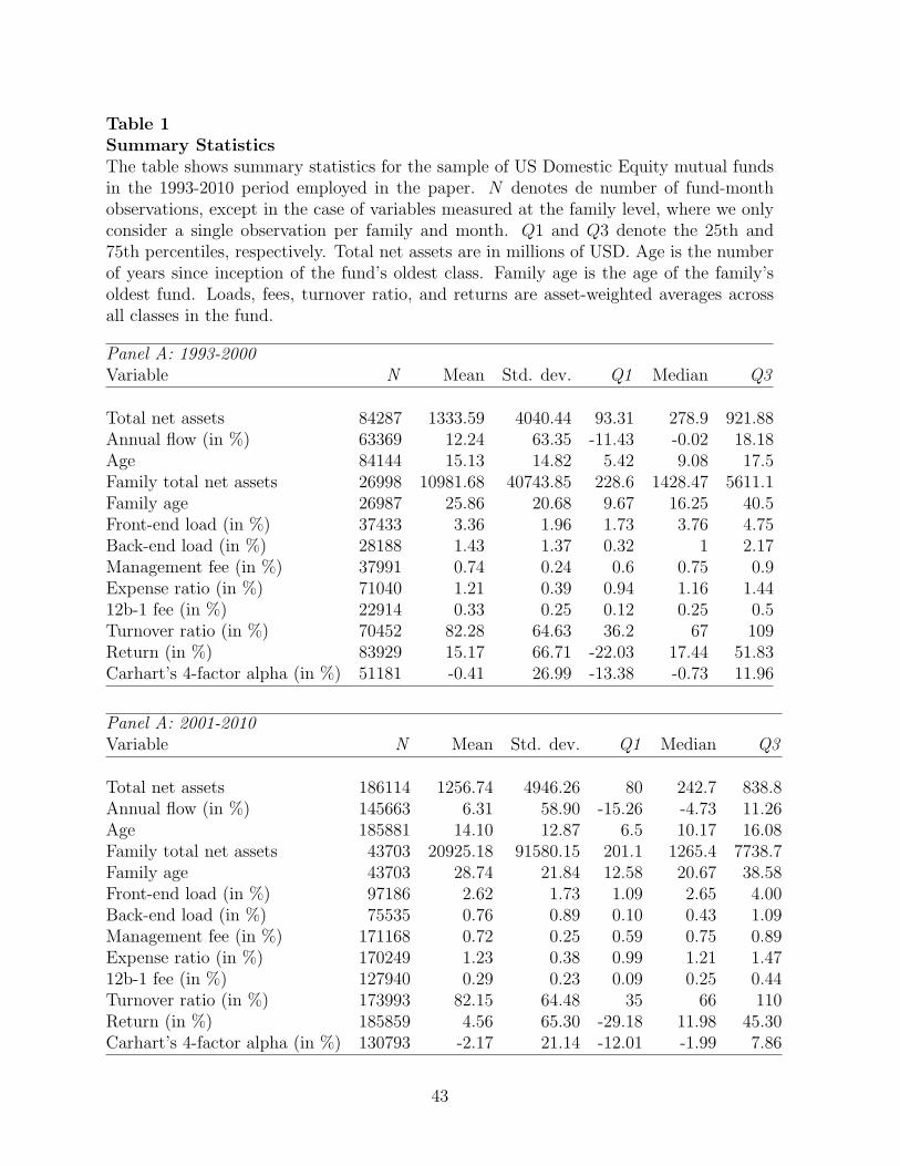
Table 1Summary StatisticsThe table shows summary statistics for the sample of US Domestic Equity mutual fundsin the 1993-2010 period employed in the paper. N denotes de number of fund-monthobservations, except in the case of variables measured at the family level, where we onlyconsider a single observation per family and month. Q1 and Q3 denote the 25th and75th percentiles, respectively. Total net assets are in millions of USD. Age is the numberof years since inception of the fund’s oldest class. Family age is the age of the family’soldest fund. Loads, fees, turnover ratio, and returns are asset-weighted averages acrossall classes in the fund.

Panel A: 1993-2000Variable N Mean Std. dev. Q1 Median Q3

Total net assets 84287 1333.59 4040.44 93.31 278.9 921.88Annual flow (in %) 63369 12.24 63.35 -11.43 -0.02 18.18Age 84144 15.13 14.82 5.42 9.08 17.5Family total net assets 26998 10981.68 40743.85 228.6 1428.47 5611.1Family age 26987 25.86 20.68 9.67 16.25 40.5Front-end load (in %) 37433 3.36 1.96 1.73 3.76 4.75Back-end load (in %) 28188 1.43 1.37 0.32 1 2.17Management fee (in %) 37991 0.74 0.24 0.6 0.75 0.9Expense ratio (in %) 71040 1.21 0.39 0.94 1.16 1.4412b-1 fee (in %) 22914 0.33 0.25 0.12 0.25 0.5Turnover ratio (in %) 70452 82.28 64.63 36.2 67 109Return (in %) 83929 15.17 66.71 -22.03 17.44 51.83Carhart’s 4-factor alpha (in %) 51181 -0.41 26.99 -13.38 -0.73 11.96

Panel A: 2001-2010Variable N Mean Std. dev. Q1 Median Q3

Total net assets 186114 1256.74 4946.26 80 242.7 838.8Annual flow (in %) 145663 6.31 58.90 -15.26 -4.73 11.26Age 185881 14.10 12.87 6.5 10.17 16.08Family total net assets 43703 20925.18 91580.15 201.1 1265.4 7738.7Family age 43703 28.74 21.84 12.58 20.67 38.58Front-end load (in %) 97186 2.62 1.73 1.09 2.65 4.00Back-end load (in %) 75535 0.76 0.89 0.10 0.43 1.09Management fee (in %) 171168 0.72 0.25 0.59 0.75 0.89Expense ratio (in %) 170249 1.23 0.38 0.99 1.21 1.4712b-1 fee (in %) 127940 0.29 0.23 0.09 0.25 0.44Turnover ratio (in %) 173993 82.15 64.48 35 66 110Return (in %) 185859 4.56 65.30 -29.18 11.98 45.30Carhart’s 4-factor alpha (in %) 130793 -2.17 21.14 -12.01 -1.99 7.86

43

Table 2Differences between Visibility SubsamplesThe table compares selected fund characteristics across fund subsamples defined accordingto fund visibility. Risk-adjusted performance is estimated using Carhart’s (1997) four-factormodel. α denotes performance in the subsequent 12 months. Assets denotes the fund’s assetsunder management. F-load and B-load denote the fund’s asset-weighted front-end load andback-end load, respectively. 12b-1 fee and Man. fee denote the fund’s 12b-1 and managementfee, respectively. High denotes the subsample of funds that belong to the top quartile of themonthly distribution of the number of investment categories in the family, family size, familyage, or family advertising. Low is defined analogously for the bottom quartile, except forfamily advertising, in which case Low denotes subsample of funds with no reported advertisingexpenditures. The number of fund-year observations is reported in parentheses.

Assets F-load 12b-1 fee Man. fee α B-load

# Inv Cat Low 525.79 0.74% 0.12% 0.84% -1.51% 0.12%

(4360) (4360) (3675) (3318) (2316) (4360)

High 2449.55 1.63% 0.22% 0.64% -1.66% 0.50%

(4238) (4238) (3806) (3494) (2621) (4238)

Low-High -1923.77 -0.89% -0.10% 0.20% 0.15% -0,38%

S.e 88.97 0.04% 0.01% 0.01% 0.20% 0.02%

Family Size Low 186.12 0.85% 0.14% 0.83% -1.55% 0.16%

(5580) (5580) (4709) (4276) (2915) (5580)

High 3387.16 1.71% 0.22% 0.63% -1.73% 0.49%

(5493) (5493) (4632) (4422) (3622) (5493)

Low-High -3201.04 -0.85% -0.08% 0.20% 0.18% -0.33%

S.e. 118.97 0.04% 0.00% 0.01% 0.18% 0.02%

Family Age Low 385.02 0.69% 0.11% 0.81% -1.63% 0.11%

(5648) (5648) (4761) (4455) (2622) (5648)

High 2971.8 2.12% 0.27% 0.63% -1.8% 0.52%

(5619) (5619) (4739) (4488) (3692) (5619)

Low-High -2586.78 -1.43% -0.15% 0.18% 0.16% -0.41%

S.e. 117.58 0.03% 0.00% 0.01% 0.18% 0.01%

Family Adv. Low 1210.00 1.38% 0.21% 0.74% -1.91% 0.37%

(15888) (15888) (14414) (13380) (9721) (15888)

High 2969.95 1.36% 0.19% 0.64% -1.07% 0.13%

(822) (822) (776) (731) (610) (822)

Low-High -1759.95 0.02% 0.02% 0.10% -0.84% 0.24%

S.e. 175.65 0.07% 0.01% 0.01% 0.30% 0.03%

44

Table 3Performance Persistence and Fund VisibilityThe table reports the estimated coefficients of monthly regressions of fund annual performance on pastannual performance and selected fund characteristics in the 1996-2010 period. Risk-adjusted performanceis estimated using Carhart’s (1997) four-factor model. α denotes performance over the prior 12 months.size denotes the natural logarithm of the fund’s assets under management, lagged one year. flow is thenet growth in fund’s assets during the last 12 months. age is the natural logarithm of the number ofmonths since the inception date of the fund’s oldest class, fam size and fam age, denote the size thefund’s family and the age of the oldest class in the fund’s family. F-load and B-load denote the fund’sasset-weighted front-end load and back-end load, lagged one year, respectively. turnover denotes thefund’s asset-weighted turnover. Regressors include month dummies. HI is a dummy variable that equalsone if the fund belongs to the top quartile of the monthly distribution of: the number of investmentcategories in the family (column 2); family size (column 3); family age (column 4); or family advertising(column 5). LO is defined analogously for the bottom quartile, except in column 4 where it equals one ifthe fund’s family has no reported advertising expenditures. Standard errors are clustered by both fundand month. ***, **, and * indicate significance at the 1%, 5%, and 10% levels, respectively

(1) (2) (3) (4) (5)#Inv Cat Family Size Family Age Family Adv.

α 0.071*** 0.085*** 0.088*** 0.090*** 0.113***(0.019) (0.022) (0.023) (0.022) (0.029)

size -0.003*** -0.003*** -0.003*** -0.002*** -0.002***(0.001) (0.001) (0.001) (0.001) (0.001)

flow -0.005** -0.005** -0.005** -0.004** -0.004**(0.002) (0.002) (0.002) (0.002) (0.002)

age 0.000 0.000 0.000 0.000 0.001(0.001) (0.001) (0.001) (0.001) (0.001)

fam size 0.001** 0.001** 0.003*** 0.001** 0.001(0.000) (0.001) (0.001) (0.000) (0.001)

fam age -0.000 -0.000 -0.000 -0.001 -0.001(0.001) (0.001) (0.001) (0.002) (0.001)

F-load 0.021 0.026 0.021 0.024 0.032(0.034) (0.034) (0.034) (0.034) (0.038)

B-load -0.329*** -0.317*** -0.335*** -0.328*** -0.315***(0.106) (0.105) (0.106) (0.105) (0.122)

exp -0.619** -0.615** -0.554** -0.637** -0.551*(0.275) (0.275) (0.277) (0.275) (0.295)

turnover -0.003* -0.003* -0.003* -0.003* -0.003(0.002) (0.002) (0.002) (0.002) (0.002)

α x LO -0.076** -0.059* -0.078*** -0.052**(0.031) (0.031) (0.030) (0.026)

α x HI -0.015 -0.018 -0.021 -0.048(0.025) (0.025) (0.022) (0.049)

LO 0.003 0.006** -0.003 -0.005***(0.002) (0.003) (0.003) (0.002)

HI 0.001 -0.004* -0.001 -0.001(0.002) (0.002) (0.002) (0.003)

Time Fixed Effects Yes Yes Yes Yes Yes

Observations 108,524 108,524 108,524 108,524 101,098Adjusted R-squared 0.074 0.075 0.075 0.074 0.076

45

Table 4Performance Persistence: The Role of Fund Size and Investment CategoriesThe table reports the estimated coefficients of monthly regressions of fund annual performance on pastannual performance and selected fund characteristics in the 1996-2010 period. Risk-adjusted performanceis estimated using Carhart’s (1997) four-factor model. α denotes performance over the prior 12 months.Controls include: size, flow, age, family size, family age, front-end and back-end loads, and portfolioturnover, as defined in Table 3. Regressors include dummy variables for months, investment categories,and interactions of investment categories with performance. HI is a dummy variable that equals one ifthe fund belongs to the top quartile of the monthly distribution of: the number of investment categoriesin the family (column 2); family size (column 3); family age (column 4); or family advertising (column5). LO is defined analogously for the bottom quartile, except in column 4 where it equals one if thefund’s family has no reported advertising expenditures. Standard errors are clustered by both fund andmonth. ***, **, and * indicate significance at the 1%, 5%, and 10% levels, respectively

(1) (2) (3) (4) (5)#Inv Cat Family Size Family Age Family Adv.

α 0.171*** 0.186*** 0.181*** 0.185*** 0.221***(0.043) (0.044) (0.044) (0.045) (0.058)

size -0.003*** -0.003*** -0.003*** -0.003*** -0.002***(0.001) (0.001) (0.001) (0.001) (0.001)

flow -0.005** -0.005** -0.005** -0.005** -0.004**(0.002) (0.002) (0.002) (0.002) (0.002)

age 0.001 0.001 0.001 0.001 0.001(0.001) (0.001) (0.001) (0.001) (0.001)

fam size 0.001*** 0.002*** 0.003*** 0.001*** 0.001*(0.000) (0.001) (0.001) (0.000) (0.000)

fam age -0.000 -0.000 -0.000 -0.000 -0.001(0.001) (0.001) (0.001) (0.002) (0.001)

F-load 0.025 0.029 0.026 0.027 0.036(0.034) (0.034) (0.034) (0.034) (0.038)

B-load -0.339*** -0.328*** -0.349*** -0.340*** -0.324***(0.103) (0.103) (0.104) (0.102) (0.117)

exp -0.622** -0.618** -0.552** -0.626** -0.567**(0.260) (0.260) (0.263) (0.259) (0.277)

turnover -0.002 -0.002 -0.002 -0.002 -0.001(0.001) (0.001) (0.001) (0.001) (0.002)

α x LO -0.096*** -0.089*** -0.088*** -0.058**(0.028) (0.031) (0.030) (0.025)

α x HI 0.005 0.019 -0.004 -0.028(0.025) (0.027) (0.022) (0.047)

LO 0.002 0.005* -0.003 -0.006***(0.002) (0.003) (0.003) (0.002)

HI 0.000 -0.003 -0.001 -0.001(0.002) (0.002) (0.002) (0.003)

α x size -0.003 -0.008 -0.016* -0.007 -0.005(0.007) (0.007) (0.009) (0.007) (0.007)

Time Fixed Effects Yes Yes Yes Yes YesInv. Cat. Fixed Effects Yes Yes Yes Yes YesInv. Cat. Interactions Yes Yes Yes Yes Yes

Observations 108,524 108,524 108,524 108,524 101,098Adjusted R-squared 0.090 0.091 0.091 0.091 0.094

46

Table 5Performance Persistence of Recent Winners and Losers: Ranking on Risk-Adjusted Per-formanceThe table reports the estimated coefficients of monthly regressions of fund annual risk-adjusted per-formance on past annual risk-adjusted performance and selected fund characteristics in the 1996-2010period. Risk-adjusted performance is estimated using Carhart’s (1997) four-factor model. α denotesperformance over the prior 12 months. dec n is a dummy variable that equals one if the fund belongsto the n-th decile of the monthly distribution of past performance. Coefficients for control variables arenot reported. Controls include: size, flow, age, family size, family age, front-end and back-end loads, andportfolio turnover, as defined in Table 3. Regressors include month dummies. HI is a dummy variablethat equals one if the fund belongs to the top quartile of the monthly distribution of: the number ofinvestment categories in the family (column 2); family size (column 3); family age (column 4); or familyadvertising (column 5). LO is defined analogously for the bottom quartile, except in column 4 where itequals one if the fund’s family has no reported advertising expenditures. Standard errors are clusteredby both fund and month. ***, **, and * indicate significance at the 1%, 5%, and 10% levels, respectively

(1) (2) (3) (4) (5)#Inv Cat Family Size Family Age Family Adv.

dec 1(α)(bottom) -0.008*** -0.012*** -0.010*** -0.009*** -0.009*(0.002) (0.003) (0.003) (0.003) (0.005)

dec 2(α) -0.004*** -0.005*** -0.003* -0.005** -0.006*(0.001) (0.002) (0.002) (0.002) (0.003)

dec 3(α) -0.003*** -0.003*** -0.003** -0.003*** -0.001(0.001) (0.001) (0.001) (0.001) (0.002)

dec 8(α) 0.003*** 0.003** 0.003** 0.003** 0.001(0.001) (0.001) (0.001) (0.001) (0.002)

dec 9(α) 0.006*** 0.006*** 0.008*** 0.007*** 0.008***(0.002) (0.002) (0.002) (0.002) (0.003)

dec 10(α)(top) 0.010*** 0.014*** 0.015*** 0.014*** 0.020***(0.003) (0.004) (0.004) (0.003) (0.006)

dec 1(α) x LO 0.012** 0.010** 0.009* 0.000(0.005) (0.005) (0.005) (0.005)

dec 2(α) x LO 0.003 -0.000 0.002 0.003(0.003) (0.003) (0.003) (0.003)

dec 3(α) x LO 0.006*** 0.003 0.007** -0.001(0.002) (0.002) (0.003) (0.002)

dec 1(α) x HI 0.006 -0.003 -0.001 0.017**(0.004) (0.004) (0.004) (0.008)

dec 2(α) x HI 0.002 -0.003 0.001 -0.002(0.003) (0.003) (0.003) (0.007)

dec 3(α) x HI -0.001 -0.001 -0.001 -0.003(0.002) (0.002) (0.002) (0.005)

dec 8(α) x LO -0.004* -0.004* -0.004 0.001(0.002) (0.002) (0.002) (0.002)

dec 9(α) x LO -0.001 -0.004 -0.004 -0.003(0.003) (0.003) (0.003) (0.003)

dec 10(α) x LO -0.016*** -0.014*** -0.011** -0.013**(0.005) (0.005) (0.005) (0.005)

dec 8(α) x HI 0.003 0.001 0.002 0.011**(0.002) (0.002) (0.002) (0.004)

dec 9(α) x HI 0.003 -0.004 -0.000 0.004(0.003) (0.003) (0.003) (0.005)

dec 10(α) x HI -0.005 -0.008 -0.007 -0.001(0.005) (0.006) (0.005) (0.010)

LO 0.004* 0.008*** -0.002 -0.003*(0.002) (0.003) (0.002) (0.002)

HI -0.000 -0.002 -0.001 -0.002(0.002) (0.002) (0.002) (0.003)

Time Fixed Effects Yes Yes Yes Yes YesControls Yes Yes Yes Yes Yes

Observations 108,524 108,524 108,524 108,524 101,098R-squared 0.076 0.077 0.078 0.077 0.079

47

Table 6Performance Persistence of Recent Winners and Losers: Ranking on Raw ReturnsThe table reports the estimated coefficients of monthly regressions of fund annual risk-adjusted perfor-mance on past annual returns and selected fund characteristics in the 1996-2010 period. Risk-adjustedperformance is estimated using Carhart’s (1997) four-factor model. ret denotes fund returns in the last12 months. dec n is a dummy variable that equals one if the fund belongs to the n-th decile of themonthly distribution of past performance. Coefficients for control variables are not reported. Controlsinclude: size, flow, age, family size, family age, front-end and back-end loads, and portfolio turnover, asdefined in Table 3. Regressors include month dummies. HI is a dummy variable that equals one if thefund belongs to the top quartile of the monthly distribution of: the number of investment categories inthe family (column 2); family size (column 3); family age (column 4); or family advertising (column 5).LO is defined analogously for the bottom quartile, except in column 4 where it equals one if the fund’sfamily has no reported advertising expenditures. Standard errors are clustered by both fund and month.***, **, and * indicate significance at the 1%, 5%, and 10% levels, respectively

(1) (2) (3) (4) (5)#Inv Cat Family Size Family Age Family Adv.

dec 1(ret) -0.009*** -0.013*** -0.012*** -0.012*** -0.009(0.003) (0.003) (0.003) (0.003) (0.005)

dec 2(ret) -0.004*** -0.006*** -0.007*** -0.004** -0.004(0.002) (0.002) (0.002) (0.002) (0.004)

dec 3(ret) -0.003** -0.004** -0.003** -0.003* 0.000(0.001) (0.002) (0.002) (0.002) (0.003)

dec 8(ret) 0.000 -0.000 -0.001 0.001 0.002(0.001) (0.002) (0.002) (0.002) (0.003)

dec 9(ret) 0.002 0.001 0.002 0.003 0.007*(0.002) (0.002) (0.002) (0.002) (0.004)

dec 10(ret) 0.003 0.003 0.003 0.005 0.006(0.003) (0.004) (0.004) (0.004) (0.006)

dec 1(ret) x LO 0.012*** 0.010** 0.012*** -0.001(0.004) (0.004) (0.005) (0.005)

dec 2(ret) x LO 0.009*** 0.008** 0.005* -0.000(0.003) (0.003) (0.003) (0.004)

dec 3(ret) x LO 0.005 0.003 0.005* -0.003(0.003) (0.003) (0.003) (0.003)

dec 1(ret) x HI 0.011** 0.001 0.003 -0.002(0.004) (0.005) (0.005) (0.010)

dec 2(ret) x HI 0.003 0.003 -0.004 -0.001(0.003) (0.003) (0.003) (0.006)

dec 3(ret) x HI 0.002 0.001 -0.003 -0.001(0.002) (0.002) (0.002) (0.005)

dec 8(ret) x LO 0.000 0.002 -0.001 -0.002(0.003) (0.002) (0.003) (0.003)

dec 9(ret) x LO 0.000 0.002 -0.003 -0.006(0.003) (0.004) (0.003) (0.004)

dec 10(ret) x LO -0.002 0.001 -0.002 -0.004(0.005) (0.005) (0.005) (0.005)

dec 8(ret) x HI 0.002 0.002 -0.003 -0.003(0.002) (0.002) (0.002) (0.005)

dec 9(ret) x HI 0.002 -0.004 -0.003 -0.004(0.003) (0.003) (0.003) (0.005)

dec 10(ret) x HI 0.002 -0.003 -0.004 -0.000(0.006) (0.005) (0.004) (0.010)

LO 0.001 0.004 -0.003 -0.003(0.002) (0.003) (0.003) (0.002)

HI -0.001 -0.004* 0.000 0.001(0.002) (0.002) (0.002) (0.003)

Time Fixed Effects Yes Yes Yes Yes YesControls Yes Yes Yes Yes Yes

Observations 108,524 108,524 108,524 108,524 101,098Adjusted R-squared 0.073 0.074 0.074 0.074 0.075

48

Table 7Other Forms of Segmentation: Retail v. Institutional Funds; and Brokered v.Directly-Sold FundsThe table reports the estimated coefficients of monthly regressions of fund annual perfor-mance on past annual performance and selected fund characteristics in the 1996-2010 period.Risk-adjusted performance is estimated using Carhart’s (1997) four-factor model. α denotesperformance over the prior 12 months. dec n is a dummy variable that equals one if the fundbelongs to the n-th decile of the monthly distribution of past performance. Coefficients forcontrol variables are not reported. Controls include: size, flow, age, family size, family age,front-end and back-end loads, and portfolio turnover, as defined in Table 3. Regressors includemonth dummies. Each regression is run on a different sample: All funds (Column 1); Retailfunds (Column 2); Institutional funds (Column 3); Brokered funds (Column 4); and Directlysold (Column 5). Standard errors are clustered by both fund and month. ***, **, and *indicate significance at the 1%, 5%, and 10% levels, respectively

(1) (2) (3) (4) (5)All Retail Instit. Broker Direct

dec 1(α)(bottom) -0.008*** -0.008*** -0.009** -0.007** -0.010***(0.002) (0.003) (0.004) (0.003) (0.003)

dec 2(α) -0.004*** -0.004*** -0.003 -0.005*** -0.003(0.001) (0.002) (0.002) (0.002) (0.002)

dec 3(α) -0.003*** -0.003*** -0.000 -0.005*** -0.000(0.001) (0.001) (0.002) (0.001) (0.001)

dec 8(α) 0.003*** 0.003*** 0.001 0.004*** 0.002(0.001) (0.001) (0.002) (0.001) (0.001)

dec 9(α) 0.006*** 0.006*** 0.008*** 0.007*** 0.006***(0.002) (0.002) (0.003) (0.002) (0.002)

dec 10(α)(top) 0.010*** 0.009*** 0.014** 0.012*** 0.007**(0.003) (0.003) (0.006) (0.004) (0.004)

Time Fixed Effects Yes Yes Yes Yes YesControls Yes Yes Yes Yes Yes

Observations 108,524 86,599 21,925 51,978 56,546Adjusted R-squared 0.076 0.077 0.099 0.092 0.065

49

Table 8Fund Visibility and Total Annual Fees (1-Year Holding Period)The table reports the estimated coefficients of annual regressions of total annual fees on past visibilitydummies and selected fund characteristics in the 1996-2010 period. Total annual fee is computed asthe sum of the expense ratio and annualized loads, assuming a 1-year holding period, and expressedin percent units. Controls include: size, age, family size, family age, portfolio turnover, annual returnvolatility, and Carhart’s (1997) risk-adjusted performance over the prior three years (annualized andexpressed in percent units). All controls are lagged one year. Regressions also include dummy variablesfor months and investment categories. HI is a dummy variable that equals one if the fund belongs to thetop quartile of the monthly distribution of: the number of investment categories in the family (column1); family size (column 2); family age (column 3); or family advertising (column 4). LO is definedanalogously for the bottom quartile, except in column 4 where it equals one if the fund’s family has noreported advertising expenditures. Standard errors are clustered by both fund and month. ***, **, and* indicate significance at the 1%, 5%, and 10% levels, respectively

(1) (2) (3) (4)#Inv Cat Family Size Family Age Family Adv.

LO -0.923*** -0.851*** -0.290** 0.494***(0.155) (0.246) (0.138) (0.160)

HI -0.296* -0.110 0.220 -0.767***(0.174) (0.188) (0.195) (0.280)

size -0.029 -0.064 -0.060 -0.069(0.047) (0.046) (0.046) (0.047)

age 0.323** 0.345*** 0.333*** 0.348***(0.126) (0.128) (0.127) (0.125)

turnover 0.016 -0.003 0.022 -0.009(0.084) (0.087) (0.086) (0.091)

fam size -0.044 -0.068 0.020 0.086**(0.047) (0.067) (0.039) (0.044)

fam age 1.080*** 1.082*** 0.886*** 1.088***(0.106) (0.109) (0.156) (0.111)

volatility 4.374 4.233 4.050 5.485**(2.827) (2.853) (2.938) (2.545)

performance -0.029*** -0.033*** -0.032*** -0.032***(0.009) (0.009) (0.009) (0.010)

Constant -3.794*** -3.760*** -3.204*** -5.875***(0.827) (0.903) (1.129) (0.752)

Time Fixed Effects Yes Yes Yes YesInv. Cat. Fixed Effects Yes Yes Yes Yes

Observations 9,370 9,358 9,370 8,372Adjusted R-squared 0.166 0.160 0.151 0.174

50

Table 9Fund Visibility and Total Annual Fees (5-Year Holding Period)The table reports the estimated coefficients of annual regressions of total annual fees on past visibilitydummies and selected fund characteristics in the 1996-2010 period. Total annual fee is computed asthe sum of the expense ratio and annualized loads, assuming a 5-year holding period, and expressedin percent units. Controls include: size, age, family size, family age, portfolio turnover, annual returnvolatility, and Carhart’s (1997) risk-adjusted performance over the prior three years (annualized andexpressed in percent units). All controls are lagged one year. Regressions also include dummy variablesfor months and investment categories. HI is a dummy variable that equals one if the fund belongs to thetop quartile of the monthly distribution of: the number of investment categories in the family (column1); family size (column 2); family age (column 3); or family advertising (column 4). LO is definedanalogously for the bottom quartile, except in column 4 where it equals one if the fund’s family has noreported advertising expenditures. Standard errors are clustered by both fund and month. ***, **, and* indicate significance at the 1%, 5%, and 10% levels, respectively

#Inv Cat Family Size Family Age Family Adv.

LO -0.213*** -0.275**** -0.113*** 0.121**(0.043) (0.061) (0.040) (0.047)

HI -0.059 0.008 0.065 -0.205***(0.048) (0.053) (0.052) (0.079)

size -0.027** -0.035*** -0.034*** -0.035***(0.013) (0.013) (0.013) (0.013)

age 0.010 0.017 0.012 0.014(0.035) (0.035) (0.035) (0.034)

turnover 0.038* 0.033 0.039* 0.032(0.023) (0.023) (0.023) (0.025)

fam size -0.050*** -0.070*** -0.036*** -0.019(0.014) (0.018) (0.011) (0.012)

fam age 0.329*** 0.328*** 0.262*** 0.334***(0.033) (0.033) (0.045) (0.034)

volatility 2.702*** 2.677*** 2.607*** 3.072***(0.868) (0.856) (0.897) (0.852)

performance -0.011*** -0.012*** -0.012*** -0.012***(0.003) (0.003) (0.003) (0.004)

Constant 0.300 0.400* 0.567* -0.277(0.230) (0.235) (0.311) (0.208)

Time Fixed Effects Yes Yes Yes YesInv. Cat. Fixed Effects Yes Yes Yes Yes

Observations 9,370 9,358 9,370 8,372Adjusted R-squared 0.144 0.145 0.135 0.153

51