False Discoveries in Mutual Fund Performance:

Measuring Luck in Estimated Alphas∗

Laurent Barras†, Olivier Scaillet‡, and Russ Wermers§

First version, September 2005; This version, May 2008

JEL Classification: G11, G23, C12Keywords: Mutual Fund Performance, Multiple-Hypothesis Test, Luck, False

Discovery Rate

∗We are grateful to S. Brown, B. Dumas, M. Huson, A. Metrick, L. Pedersen, E. Ronchetti,R. Stulz, M.-P. Victoria-Feser, M. Wolf, as well as seminar participants at Banque Cantonalede Genève, BNP Paribas, Bilgi University, CREST, Greqam, INSEAD, London School of Eco-nomics, Maastricht University, MIT, Princeton University, Queen Mary, Solvay Business School,NYU (Stern School), Universita della Svizzera Italiana, University of Geneva, University of Geor-gia, University of Missouri, University of Notre-Dame, University of Pennsylvania, Universityof Virginia (Darden), the Imperial College Risk Management Workshop (2005), the Swiss Doc-toral Workshop (2005), the Research and Knowledge Transfer Conference (2006), the ZeuthenFinancial Econometrics Workshop (2006), the Professional Asset Management Conference atRSM Erasmus University (2008), the Joint University of Alberta/University of Calgary FinanceConference (2008), the annual meetings of EC2 (2005), ESEM (2006), EURO XXI (2006), ICA(2006), AFFI (2006), SGF (2006), and WHU Campus for Finance (2007) for their helpful com-ments. We also thank C. Harvey (the Editor), the Associate Editor and the Referee (bothanonymous) for numerous helpful insights. The first and second authors acknowledge finan-cial support by the National Centre of Competence in Research “Financial Valuation and RiskManagement” (NCCR FINRISK). Part of this research was done while the second author wasvisiting the Centre Emile Bernheim (ULB).

†Swiss Finance Institute and Imperial College, Tanaka Business School, London SW7 2AZ,UK. Tel: +442075949766. E-mail: l.barras@ic.ac.uk

‡Swiss Finance Institute at HEC-University of Geneva, Boulevard du Pont d’Arve 40, 1211Geneva 4, Switzerland. Tel: +41223798816. E-mail: scaillet@hec.unige.ch

§University of Maryland - Robert H. Smith School of Business, Department of Finance,College Park, MD 20742-1815, Tel: +13014050572. E-mail: wermers@umd.edu

ABSTRACT

This paper uses a new approach to determine the fraction of truly skilled managers

among the universe of U.S. domestic-equity mutual funds over the 1975 to 2006 period.

We develop a simple technique that properly accounts for “false discoveries,” or mutual

funds which exhibit significant alphas by luck alone. We use this technique to precisely

separate actively managed funds into those having (1) unskilled, (2) zero-alpha, and (3)

skilled fund managers, net of expenses, even with cross-fund dependencies in estimated

alphas. This separation into skill groups allows several new insights. First, we find

that the majority of funds (75.4%) pick stocks well enough to cover their trading costs

and other expenses, producing a zero alpha, consistent with the equilibrium model of

Berk and Green (2004). Further, we find a significant proportion of skilled (positive

alpha) funds prior to 1995, but almost none by 2006, accompanied by a large increase in

unskilled (negative alpha) fund managers—due both to a large reduction in the proportion

of fund managers with stockpicking skills and to a persistent level of expenses that

exceed the value generated by these managers. Finally, we show that controlling for false

discoveries substantially improves the ability to find funds with persistent performance.

Investors and academic researchers have long searched for outperforming mutual

fund managers. Although several researchers document negative average fund alphas,

net of expenses and trading costs (e.g., Jensen (1968), Lehman and Modest (1987), El-

ton et al. (1993), and Carhart (1997)), recent papers show that some fund managers

have stock-selection skills. For instance, Kosowski, Timmermann, Wermers, and White

(2006; KTWW) use a bootstrap technique to document outperformance by some funds,

while Baks, Metrick, and Wachter (2001), Pastor and Stambaugh (2002b), and Avramov

and Wermers (2006) illustrate the benefits of investing in actively-managed funds from

a Bayesian perspective. While these papers are useful in uncovering whether, on the

margin, outperforming mutual funds exist, they are not particularly informative regard-

ing their prevalence in the entire fund population. For instance, it is natural to wonder

how many fund managers possess true stockpicking skills, and where these funds are

located in the cross-sectional estimated alpha distribution. From an investment per-

spective, precisely locating skilled funds maximizes our chances of achieving persistent

outperformance.1

Of course, we cannot observe the true alpha of each fund in the population. There-

fore, a seemingly reasonable way to estimate the prevalence of skilled fund managers

is to simply count the number of funds with sufficiently high estimated alphas, bα. Inimplementing such a procedure, we are actually conducting a multiple (hypothesis) test,

since we simultaneously examine the performance of several funds in the population (in-

stead of just one fund).2 However, it is clear that this simple count of significant-alpha

funds does not properly adjust for luck in such a multiple test setting—many of the funds

have significant estimated alphas by luck alone (i.e., their true alphas are zero). To illus-

trate, consider a population of funds with skills just sufficient to cover trading costs and

expenses (zero-alpha funds). With the usual chosen significance level of 5%, we should

expect that 5% of these zero-alpha funds will have significant estimated alphas—some

of them will be unlucky (bα < 0) while others are lucky (bα > 0), but all will be “false

discoveries”—funds with significant estimated alphas, but zero true alphas.

This paper implements a new approach to controlling for false discoveries in such a

multiple fund setting. Our approach much more accurately estimates (1) the proportions

of unskilled and skilled funds in the population (those with truly negative and positive

1From an investor perspective, “skill” is manager talent in selecting stocks sufficient to generate apositive alpha, net of trading costs and fund expenses.

2This multiple test should not be confused with the joint hypothesis test with the null hypothesisthat all fund alphas are equal to zero in a sample. This test, which is employed by several papers (e.g.,Grinblatt and Titman (1989, 1993)), addresses only whether at least one fund has a non-zero alphaamong several funds, but is silent on the prevalence of these non-zero alpha funds.

1

alphas, respectively), and (2) their respective locations in the left and right tails of

the cross-sectional estimated alpha (or estimated alpha t-statistic) distribution. One

main virtue of our approach is its simplicity—to determine the proportions of unlucky

and lucky funds, the only parameter needed is the proportion of zero-alpha funds in the

population, π0. Rather than arbitrarily imposing a prior assumption on π0, our approach

estimates it with a straightforward computation that uses the p-values of individual fund

estimated alphas—no further econometric tests are necessary. A second advantage of our

approach is its accuracy. Using a simple Monte-Carlo experiment, we demonstrate that

our approach provides a much more accurate partition of the universe of mutual funds

into zero-alpha, unskilled, and skilled funds than previous approaches that impose an a

priori assumption about the proportion of zero-alpha funds in the population.3

Another important advantage of our approach to multiple testing is its robustness

to cross-sectional dependencies among fund estimated alphas. Prior literature has indi-

cated that such dependencies, which exist due to herding and other correlated trading

behaviors (e.g., Wermers (1999)), greatly complicate performance measurement in a

group setting. However, Monte Carlo simulations show that our simple approach, which

requires only the (alpha) p-value for each fund in the population—and not the estimation

of the cross-fund covariance matrix—is quite robust to such dependencies.

We apply our novel approach to the monthly returns of 2,076 actively managed U.S.

open-end, domestic-equity mutual funds that exist at any time between 1975 and 2006

(inclusive), and revisit several important themes examined in the previous literature.

We start with an examination of the long-term (lifetime) performance (net of trading

costs and expenses) of these funds. Our decomposition of the population reveals that

75.4% are zero-alpha funds—funds having managers with some stockpicking abilities, but

that extract all of the rents generated by these abilities through fees. Among remaining

funds, only 0.6% are skilled (true α > 0), while 24.0% are unskilled (true α < 0).While

our empirical finding that the majority are zero-alpha funds is supportive of the long-

run equilibrium theory of Berk and Green (2004), it is surprising that we find so many

truly negative-alpha funds—those that overcharge relative to the skills of their managers.

Indeed, we find that such unskilled funds underperform for long time periods, indicating

that investors have had some time to evaluate and identify them as underperformers.

We also find some notable time trends in our study. Examining the evolution of

3The reader should note the difference between our approach and that of KTWW (2006). Ourapproach simultaneously estimates the prevalence and location of outperforming funds in a group, whileKTWW test for the skills of a single fund that is chosen from the universe of alpha-ranked funds. Assuch, our approach examines fund performance from a more general perspective, with a richer set ofinformation about active fund manager skills.

2

each skill group between 1990 and 2006, we observe that the proportion of skilled funds

dramatically decreases from 14.4% to 0.6%, while the proportion of unskilled funds

increases sharply from 9.2% to 24.0%. Thus, although the number of actively managed

funds has dramatically increased, skilled managers (those capable of picking stocks well

enough to overcome their trading costs and expenses) have become increasingly rare.

Motivated by the possibility that funds may outperform over the short-run, before

investors compete away their performance with inflows, we conduct further tests over

five-year subintervals—treating each five-year fund record as a separate “fund.” Here, we

find that the proportion of skilled funds equals 2.4%, implying that a small number of

managers have “hot hands” over short time periods. These skilled funds are located in

the extreme right tail of the cross-sectional estimated alpha distribution, which indicates

that a very low p-value is an accurate signal of short-run fund manager skill (relative to

pure luck). Across the investment subgroups, Aggressive Growth funds have the highest

proportion of managers with short-term skills, while Growth & Income funds exhibit no

skills.

The concentration of skilled funds in the extreme right tail of the estimated alpha

distribution suggests a natural way to choose funds in seeking out-of-sample persistent

performance. Specifically, we form portfolios of right-tail funds that condition on the

frequency of “false discoveries”—during years when our tests indicate higher proportions

of lucky, zero-alpha funds in the right tail, we move further to the extreme tail to

decrease false discoveries. Forming such a false discovery controlled portfolio at the

beginning of each year from January 1980 to 2006, we find a four-factor alpha of 1.45%

per year, which is statistically significant. Notably, we show that this luck-controlled

strategy outperforms prior persistence strategies used by Carhart (1997) and others,

where constant top-decile portfolios of funds are chosen with no control for luck.

Our final tests examine the performance of fund managers before expenses (but after

trading costs) are subtracted. Specifically, while fund managers may be able to pick

stocks well enough to cover their trading costs, they usually do not exert direct control

over the level of fund expenses and fees—management companies set these expenses, with

the approval of fund directors. We find evidence that indicates a very large impact of

fund fees and other expenses. Specifically, on a pre-expense basis, we find a much higher

incidence of funds with positive alphas—9.6%, compared to our above-mentioned finding

of 0.6% after expenses. Thus, almost all outperforming funds appear to capture (or waste

through operational inefficiencies) the entire surplus created by their portfolio managers.

It is also noteworthy that the proportion of skilled managers (before expenses) declines

substantially over time, again indicating that portfolio managers with skills have become

3

increasingly rare. We also observe a large reduction in the proportion of unskilled funds

when we move from net alphas to pre-expense alphas (from 24.0% to 4.5%), indicating

a big role for excessive fees (relative to manager stockpicking skills) in underperforming

funds. Although industry sources argue that competition among funds has reduced fees

and expenses substantially since 1980 (Rea and Reid (1998)), our study indicates that a

large subgroup of investors appear to either be unaware that they are being overcharged

(Christoffersen and Musto (2002)), or are constrained to invest in high-expense funds

(Elton, Gruber, and Blake (2007)).

The remainder of the paper is as follows. The next section explains our approach

to separating luck from skill in measuring the performance of asset managers. Section

2 presents the performance measures, and describes the mutual fund data. Section 3

contains the results of the paper, while Section 4 concludes.

I The Impact of Luck on Mutual Fund Performance

A Overview of the Approach

A.1 Luck in a Multiple Fund Setting

Our objective is to develop a framework to precisely estimate the fraction of mutual

funds in a large group that truly outperform their benchmarks. To begin, suppose

that a population of M actively managed mutual funds is composed of three distinct

performance categories, where performance is due to stock-selection skills. We define

such performance as the ability of fund managers to generate superior model alphas,

net of trading costs as well as all fees and other expenses (except loads and taxes). Our

performance categories are defined as follows:

• Unskilled funds: funds having managers with stockpicking skills insufficient torecover their trading costs and expenses, creating an “alpha shortfall” (α < 0),

• Zero-alpha funds: funds having managers with stockpicking skills sufficient tojust recover trading costs and expenses (α = 0),

• Skilled funds: funds having managers with stockpicking skills sufficient to pro-vide an “alpha surplus,” beyond simply recovering trading costs and expenses (α > 0).

Note that our above definition of skill is one that is relative to expenses, and not in

an absolute sense. This definition is driven by the idea that consumers look for mutual

funds that deliver surplus alpha, net of all expenses.4

4However, perhaps a manager exhibits skill sufficient to more than compensate for trading costs,but the fund management company overcharges fees or inefficiently generates other services (such asadministrative services, e.g., record-keeping)—costs that the manager usually has little control over. In

4

Of course, we cannot observe the true alphas of each fund in the population. There-

fore, how do we best infer the prevalence of each of the above skill groups from perfor-

mance estimates for individual funds? First, we use the t-statistic, bti = bαi/bσbαi , as ourperformance measure, where bαi is the estimated alpha for fund i, and bσbαi is its estimatedstandard deviation—KTWW (2006) show that the t-statistic has superior properties rel-

ative to alpha, since alpha estimates have differing precision across funds with varying

lives and portfolio volatilities. Second, after choosing a significance level, γ (e.g., 10%),

we observe whether bti lies outside the thresholds implied by γ (denoted by t−γ and t+γ ),

and label it “significant” if it is such an outlier. This procedure, simultaneously applied

across all funds, is a multiple-hypothesis test:

H0,1 : α1 = 0, HA,1 : α1 6= 0,... : ...

H0,M : αM = 0, HA,M : αM 6= 0. (1)

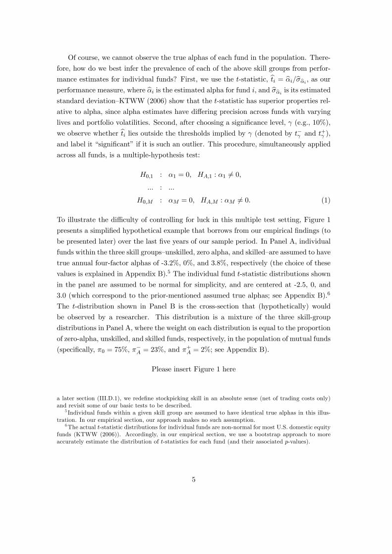
To illustrate the difficulty of controlling for luck in this multiple test setting, Figure 1

presents a simplified hypothetical example that borrows from our empirical findings (to

be presented later) over the last five years of our sample period. In Panel A, individual

funds within the three skill groups—unskilled, zero alpha, and skilled—are assumed to have

true annual four-factor alphas of -3.2%, 0%, and 3.8%, respectively (the choice of these

values is explained in Appendix B).5 The individual fund t-statistic distributions shown

in the panel are assumed to be normal for simplicity, and are centered at -2.5, 0, and

3.0 (which correspond to the prior-mentioned assumed true alphas; see Appendix B).6

The t-distribution shown in Panel B is the cross-section that (hypothetically) would

be observed by a researcher. This distribution is a mixture of the three skill-group

distributions in Panel A, where the weight on each distribution is equal to the proportion

of zero-alpha, unskilled, and skilled funds, respectively, in the population of mutual funds

(specifically, π0 = 75%, π−A = 23%, and π+A = 2%; see Appendix B).

Please insert Figure 1 here

a later section (III.D.1), we redefine stockpicking skill in an absolute sense (net of trading costs only)and revisit some of our basic tests to be described.

5 Individual funds within a given skill group are assumed to have identical true alphas in this illus-tration. In our empirical section, our approach makes no such assumption.

6The actual t-statistic distributions for individual funds are non-normal for most U.S. domestic equityfunds (KTWW (2006)). Accordingly, in our empirical section, we use a bootstrap approach to moreaccurately estimate the distribution of t-statistics for each fund (and their associated p-values).

5

To illustrate further, suppose that we choose a significance level, γ, of 10% (correspond-

ing to t−γ = −1.65 and t+γ = 1.65). With the test shown in Equation (1), the researcher

would expect to find 5.4% of funds with a positive and significant t-statistic.7 This pro-

portion, denoted by E(S+γ ), is represented by the shaded region in the right tail of the

cross-sectional t-distribution (Panel B). Does this area consist merely of skilled funds, as

defined above? Clearly not, because some funds are just lucky; as shown in the shaded

region of the right tail in Panel A, zero-alpha funds can exhibit positive and significant

estimated t-statistics. By the same token, the proportion of funds with a negative and

significant t-statistic (the shaded region in the left-tail of Panel B) overestimates the

proportion of unskilled funds, because it includes some unlucky zero-alpha funds (the

shaded region in the left tail in Panel A). Note that we have not considered the possi-

bility that skilled funds could be very unlucky, and exhibit a negative and significant

t-statistic. In our example of Figure 1, the probability that the estimated t-statistic of a

skilled fund is lower than t−γ = −1.65 is less than 0.001%. This probability is negligible,so we ignore this pathological case. The same applies to unskilled funds that are very

lucky.

The message conveyed by Figure 1 is that we measure performance with a limited

sample of data, therefore, unskilled and skilled funds cannot easily be distinguished from

zero-alpha funds. This problem can be worse if the cross-section of actual skill levels has

a complex distribution (and not all fixed at the same levels, as assumed by our simplified

example), and is further compounded if a substantial proportion of skilled fund managers

have low levels of skill, relative to the error in estimating their t-statistics. To proceed,

we must employ a procedure that is able to precisely account for “false discoveries,” i.e.,

funds that falsely exhibit significant estimated alphas (i.e., their true alphas are zero)

in the face of these complexities.

A.2 Measuring Luck

How do we measure the frequency of “false discoveries” in the tails of the cross-sectional

(alpha) t-distribution? At a given significance level γ, it is clear that the probability

that a zero-alpha fund (as defined in the last section) exhibits luck equals γ/2 (shown as

the dark shaded region in Panel A of Figure 1)). If the proportion of zero-alpha funds in

the population is π0, the expected proportion of “lucky funds” (zero-alpha funds with

7From Panel A, the probability that the observed t-statistic is greater than t+γ = 1.65 equals 5%for a zero-alpha fund and 84% for a skilled fund. Multiplying these two probabilities by the respectiveproportions represented by their categories (π−A and π+A) gives 5.4%.

6

positive and significant t-statistics) equals

E(F+γ ) = π0 · γ/2. (2)

Now, to determine the expected proportion of skilled funds, E(T+γ ), we simply adjust

E(S+γ ) for the presence of these lucky funds:

E(T+γ ) = E(S+γ )−E(F+γ ) = E(S+γ )− π0 · γ/2. (3)

Since the probability of a zero-alpha fund being unlucky is also equal to γ/2 (i.e., the grey

and black areas in Panel A of Figure 1 are identical), E(F−γ ), the expected proportion

of “unlucky funds,” is equal to E(F+γ ). As a result, the expected proportion of unskilled

funds, E(T−γ ), is similarly given by

E(T−γ ) = E(S−γ )−E(F−γ ) = E(S−γ )− π0 · γ/2. (4)

What is the role played by the significance level, γ, chosen by the researcher? By

defining the significance thresholds t−γ and t+γ , γ determines the portion of the right (or

left) tail which is examined for lucky vs. skilled funds (or unlucky vs. unskilled funds),

as described by Equations (3) and (4). By varying γ, we can determine the location of

skilled (or unskilled) funds—by measuring the proportion of such funds in any segment

of the cross-section.

This flexibility in choosing γ provides us with opportunities to make important in-

sights into the merits of active fund management. First, by choosing a larger γ (i.e., lower

t−γ and t+γ , in absolute value), we can estimate the proportions of unskilled and skilled

funds in a larger portion of the left and right tails of the cross-sectional t-distribution,

respectively—thus, giving us an appreciation of the proportions of unskilled and skilled

funds in the entire population, π−A and π+A. That is, as we increase γ, E(T

−γ ) and E(T

+γ )

converge to π−A and π+A, thus minimizing Type II error (failing to locate truly unskilled

or skilled funds). Alternatively, by reducing γ, we can determine the precise location of

unskilled or skilled funds in the extreme tails of the t-distribution. For instance, choos-

ing a very low γ (i.e., very large t−γ and t+γ , in absolute value) allows us to determine

whether extreme tail funds are skilled or simply lucky (unskilled or simply unlucky)—

information that is quite useful to investors trying to locate skilled (or avoid unskilled)

managers.

7

A.3 Estimation Procedure

The key to our approach to measuring luck in a group setting, as shown in Equation

(2), is the estimator of the proportion, π0, of zero-alpha funds in the population. Here,

we turn to a recent estimation approach developed by Storey (2002)—called the “False

Discovery Rate” (FDR) approach. The FDR approach is very straightforward, as its

sole inputs are the (two-sided) p-values associated with the (alpha) t-statistics of each of

the M funds. By definition, zero-alpha funds satisfy the null hypothesis, H0,i : αi = 0,

and, therefore, have p-values that are uniformly distributed over the interval [0, 1] .8 On

the other hand, p-values of unskilled and skilled funds tend to be very small because

their estimated t-statistics tend to be far from zero (see Panel A of Figure 1). We can

exploit this information to estimate π0 without knowing the exact distribution of the

p-values of the unskilled and skilled funds.

To explain further, a key intuition of the FDR approach is that it uses information

from the center of the cross-sectional t-distribution (which is dominated by zero-alpha

funds) to correct for luck in the tails. To illustrate the FDR procedure, suppose we

randomly draw 2,076 t-statistics (the number of funds in our study), each from one of

the three t-distributions in Panel A of Figure 1. Each t-statistic is drawn from a given

distribution with probability according to our estimates of the proportion of unskilled,

zero-alpha, and skilled funds in the population, π0 = 75%, π−A = 23%, and π+A = 2%,

respectively. Thus, our draw of t-statistics comes from a known frequency of each type

(23%, 75%, and 2%). Next, we apply the FDR technique to estimate these frequencies—

from the sampled t-statistics, we compute two-sided p-values, bpi, for each of the 2,076funds, then plot them in Figure 2.

Please insert Figure 2 here

The darkest grey zone near zero captures the majority of p-values of unskilled and skilled

funds (π−A + π+A =25%). The area below the horizontal line at 0.075 represents the true

(but unknown to the researcher) proportion, π0, of zero-alpha funds (75%), since zero-

alpha funds have uniformly distributed p-values. The researcher estimates π0 from the

histogram of observed p-values as follows. If we take a sufficiently high threshold λ∗

(e.g., λ∗ = 0.6), we know that the vast majority of p-values higher than λ∗ come from

8To see this, let us denote by t and p the t-statistic and p-value of the zero-alpha fund. We have p =1−F (|t|), where F (t) = prob(

¯̄bti ¯̄ < |t|¯̄αi = 0). The p-value is uniformly distributed over [0, 1] since itscdf, G(p) = prob(bpi < p) = prob(1−F (|tbpi |) < p) = prob(|tbpi | > F−1 (1− p)) = 1−F

¡F−1 (1− p)

¢= p.

8

zero-alpha funds. Thus, we first measure the proportion of the total area that is covered

by the four lightest grey bars on the right of λ∗, cW (λ∗) /M (where cW (λ∗) denotes the

number of funds having p-values exceeding λ∗). Then, we extrapolate this area over the

entire interval [0, 1] by multiplying by 1/(1−λ∗) (e.g., if λ∗ = 0.6, the area is multipliedby 2.5):9

bπ0 (λ∗) = cW (λ∗)

M· 1

(1− λ∗). (5)

To select λ∗, we use the simple data-driven approach suggested by Storey (2002) and

explained in detail in Appendix A.

Substituting the estimate bπ0 in Equations (2), (3), and replacing E(S+γ ) with the

observed proportion of significant funds in the right tail, bS+γ , we can easily estimateE(F+γ ) and E(T

+γ ) corresponding to any chosen significance level, γ. The same approach

can be used in the left tail by replacing E(S−γ ) in Equation (4) with the observed

proportion of significant funds in the left tail, bS−γ . This implies the following estimatesof the proportions of unlucky and lucky funds:

bF−γ = bF+γ = bπ0 · γ/2. (6)

Using Equation (6), the estimated proportions of unskilled and skilled funds (at the

chosen significance level, γ) are, respectively, equal to

bT−γ = bS−γ − bF−γ = bS−γ − bπ0 · γ/2,bT+γ = bS+γ − bF+γ = bS+γ − bπ0 · γ/2. (7)

Finally, we estimate the proportions of unskilled and skilled funds in the entire popula-

tion as bπ−A = bT−γ∗ , bπ+A = bT+γ∗ , (8)

where γ∗ is a sufficiently high significance level—we choose γ∗ with a simple data-driven

method explained in Appendix A.

B Comparison of Our Approach with Existing Methods

The previous literature has followed two alternative approaches when estimating the

proportions of unskilled and skilled funds. The “full luck” approach proposed by Jensen9This estimation procedure cannot be used in a one-sided multiple test, since the null hypothesis is

tested under the least favorable configuration (LFC). For instance, consider the following null hypothesisH0,i : αi ≤ 0. Under the LFC, it is replaced with H0,i : αi = 0. Therefore, all funds with αi ≤ 0 (i.e.,drawn from the null) have inflated p-values which are not uniformly distributed over [0, 1].

9

(1968) and Ferson and Qian (2004) assumes, a priori, that all funds in the population

have zero alphas, π0 = 1. Thus, for a given significance level, γ, this approach implies

an estimate of the proportions of unlucky and lucky funds equal to γ/2.10 At the other

extreme, the “no luck” approach reports the observed number of significant funds (for

instance, Ferson and Schadt (1996)) without making a correction for luck.

What are the errors introduced by assuming, a priori, that π0 equals 0 or 1, when it

does not accurately describe the population? To address this question, we compare the

bias produced by these two approaches relative to our FDR approach across different

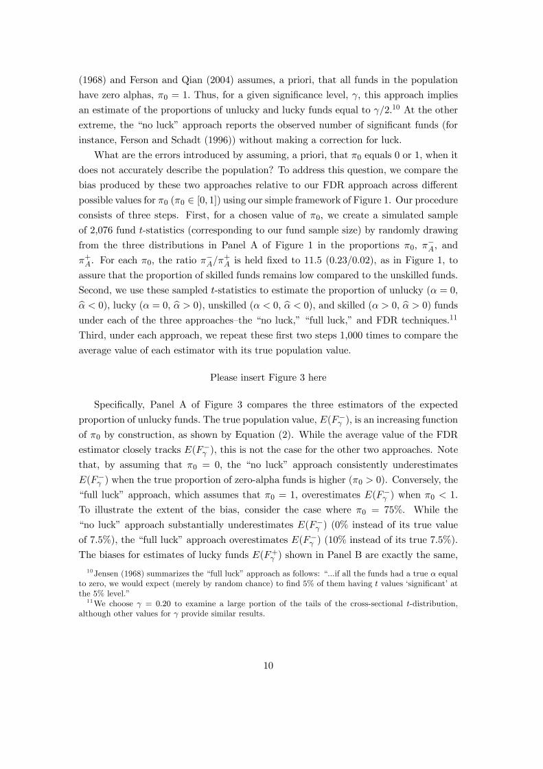
possible values for π0 (π0 ∈ [0, 1]) using our simple framework of Figure 1. Our procedureconsists of three steps. First, for a chosen value of π0, we create a simulated sample

of 2,076 fund t-statistics (corresponding to our fund sample size) by randomly drawing

from the three distributions in Panel A of Figure 1 in the proportions π0, π−A, and

π+A. For each π0, the ratio π−A/π+A is held fixed to 11.5 (0.23/0.02), as in Figure 1, to

assure that the proportion of skilled funds remains low compared to the unskilled funds.

Second, we use these sampled t-statistics to estimate the proportion of unlucky (α = 0,bα < 0), lucky (α = 0, bα > 0), unskilled (α < 0, bα < 0), and skilled (α > 0, bα > 0) funds

under each of the three approaches—the “no luck,” “full luck,” and FDR techniques.11

Third, under each approach, we repeat these first two steps 1,000 times to compare the

average value of each estimator with its true population value.

Please insert Figure 3 here

Specifically, Panel A of Figure 3 compares the three estimators of the expected

proportion of unlucky funds. The true population value, E(F−γ ), is an increasing function

of π0 by construction, as shown by Equation (2). While the average value of the FDR

estimator closely tracks E(F−γ ), this is not the case for the other two approaches. Note

that, by assuming that π0 = 0, the “no luck” approach consistently underestimates

E(F−γ ) when the true proportion of zero-alpha funds is higher (π0 > 0). Conversely, the

“full luck” approach, which assumes that π0 = 1, overestimates E(F−γ ) when π0 < 1.

To illustrate the extent of the bias, consider the case where π0 = 75%. While the

“no luck” approach substantially underestimates E(F−γ ) (0% instead of its true value

of 7.5%), the “full luck” approach overestimates E(F−γ ) (10% instead of its true 7.5%).

The biases for estimates of lucky funds E(F+γ ) shown in Panel B are exactly the same,

10Jensen (1968) summarizes the “full luck” approach as follows: “...if all the funds had a true α equalto zero, we would expect (merely by random chance) to find 5% of them having t values ‘significant’ atthe 5% level.”11We choose γ = 0.20 to examine a large portion of the tails of the cross-sectional t-distribution,

although other values for γ provide similar results.

10

since E(F+γ ) = E(F−γ ).

Estimates of the expected proportions of unskilled and skilled funds (E(T−γ ) and

E(T+γ )) provided by the three approaches are shown in Panels C and D, respectively.

As we move to higher true proportions of zero-alpha funds (a higher value of π0), the true

proportions of unskilled and skilled funds, E(T−γ ) and E(T+γ ), decrease by construction.

In both panels, our FDR estimator accurately captures this feature, while the other

approaches do not fare well due to their fallacious assumptions about the prevalence of

luck. For instance, when π0 = 75%, the “no luck” approach exhibits a large upward bias

in its estimates of the total proportion of unskilled and skilled funds, E(T−γ ) + E(T+γ )

(37.3% rather than the correct value of 22.3%). At the other extreme, the “full luck”

approach underestimates E(T−γ ) +E(T+γ ) (17.8% instead of 22.3%).

Panel D reveals that the “no luck” and “full luck” approaches also exhibit a non-

sensical positive relation between π0 and E(T+γ ). This result is a consequence of the

low proportion of skilled funds in the population. First, as π0 rises, the additional

lucky funds drive the proportion of significant funds up, making the “no-luck” approach

wrongly believe that more skilled funds are present. Second, the few skilled funds in the

population cannot offset the excessive luck adjustment made by the “full luck” approach,

which actually produces negative estimates of E(T+γ ).

In addition to the bias properties exhibited by our FDR estimators, their variability

is low because of the large cross-section of funds (M = 2, 076). To understand this,

consider our main estimator bπ0 (the same arguments apply to the other estimators).Since bπ0 is a proportion estimator that depends on the proportion of bpi > λ∗, the Law

of Large Numbers drives it close to its true value with our large sample size. For instance,

taking λ∗ = 0.6 and π0 = 75%, σπ0 is as low as 2.5% with independent p-values (1/30th

the magnitude of π0).12 In the appendix, we provide further evidence of the remarkable

accuracy of our estimators using Monte-Carlo simulations.

C Estimation under Cross-Sectional Dependence among Funds

Mutual funds can have correlated residuals if they “herd” in their stockholdings (Wer-

mers (1999)) or hold similar industry allocations. In general, cross-sectional dependence

in fund estimated alphas greatly complicates performance measurement. Any inference

test with dependencies becomes quickly intractable as M rises, since this requires the

12Specifically, bπ0 = (1− λ∗)−1 ·1/MPM

i=1 xi, where xi follows a binomial distribution with probabilityof success Pλ∗ = prob(bpi > λ∗) = 0.30 (i.e., the rectangle area delimited by the horizontal black line

and the vertical line at λ∗ = 0.6 in Figure 2). Therefore, we have σx = (Pλ∗ (1− Pλ∗))12 = 0.46, and

σπ0 = (1− λ∗)−1 · σx/√M = 2.5%.

11

estimation and inversion of an M ×M residual covariance matrix. In a Bayesian frame-

work, Jones and Shanken (2005) show that performance measurement requires intensive

numerical methods when investor prior beliefs about fund alphas include cross-fund de-

pendencies. Further, KTWW (2006) show that a complicated bootstrap is necessary to

test the significance of performance of a fund located at a particular alpha rank, since

this test depends on the joint distribution of all fund estimated alphas—cross-correlated

fund residuals must be bootstrapped simultaneously.

An important advantage of our approach is that we estimate the p-value of each fund

in isolation—avoiding the complications that arise because of the dependence structure

of fund residuals. However, high cross-sectional dependencies could potentially bias

our estimators. To illustrate this point with an extreme case, suppose that all funds

produce zero alphas (π0 = 100%), and that fund residuals are perfectly correlated

(perfect herding). In this case, all fund p-values would be the same, and the p-value

histogram would not converge to the uniform distribution, as shown in Figure 2. Clearly,

we would make serious errors no matter where we set λ∗.

In our sample, we are not overly concerned with dependencies, since we find that the

average correlation between four-factor model residuals of pairs of funds is only 0.08.

Further, many of our funds do not have highly overlapping return data, thus, ruling

out highly correlated residuals by construction. Specifically, we find that 15% of the

funds pairs do not have a single monthly return observation in common; on average,

only 55% of the return observations of fund pairs is overlapping. As a result, we believe

that cross-sectional dependencies are sufficiently low to allow consistent estimators (i.e.,

mutual fund residuals satisfy the ergodicity conditions discussed in Storey, Taylor, and

Siegmund (2004)).

However, in order to explicitly verify the properties of our estimators, we run a

Monte-Carlo simulation. In order to closely reproduce the actual pairwise correlations

between funds in our dataset, we estimate the residual covariance matrix directly from

the data, then use these dependencies in our simulations. In further simulations, we

impose other types of dependencies, such as residual block correlations or residual factor

dependencies, as in Jones and Shanken (2005). In all simulations, we find both that

average estimates (for all of our estimators) are very close to their true values, and that

confidence intervals for estimates are comparable to those that result from simulations

where independent residuals are assumed. These results, as well as further details on

the simulation experiment are discussed in Appendix B.

12

II Performance Measurement and Data Description

A Asset Pricing Models

To compute fund performance, our baseline asset pricing model is the four-factor model

proposed by Carhart (1997):

ri,t = αi + bi · rm,t + si · rsmb,t + hi · rhml,t +mi · rmom,t + εi,t, (9)

where ri,t is the month t excess return of fund i over the riskfree rate (proxied by the

monthly T-bill rate); rm,t is the month t excess return on the value-weighted market

portfolio; and rsmb,t, rhml,t, and rmom,t are the month t returns on zero-investment factor-

mimicking portfolios for size, book-to-market, and momentum obtained from Kenneth

French’s website.

We also implement a conditional four-factor model to account for time-varying ex-

posure to the market portfolio (Ferson and Schadt (1996)),

ri,t = αi + bi · rm,t + si · rsmb,t + hi · rhml,t +mi · rmom,t +B0(zt−1 · rm,t) + εi,t, (10)

where zt−1 denotes the J × 1 vector of centered predictive variables, and B is the J × 1vector of coefficients. The four predictive variables are the one-month T-bill rate; the

dividend yield of the CRSP value-weighted NYSE/AMEX stock index; the term spread,

proxied by the difference between yields on 10-year Treasurys and three-month T-bills;

and the default spread, proxied by the yield difference between Moody’s Baa-rated and

Aaa-rated corporate bonds. We have also computed fund alphas using the CAPM and

the Fama-French (1993) models. These results are summarized in Section III.D.2.

To compute each fund t-statistic, we use the Newey-West (1987) heteroscedastic-

ity and autocorrelation consistent estimator of the standard deviation, bσbαi . Further,KTWW (2006) find that the finite-sample distribution of bt is non-normal for approxi-mately half of the funds. Therefore, we use a bootstrap procedure (instead of asymptotic

theory) to compute fund p-values. In order to estimate the distribution of bti for eachfund i under the null hypothesis αi = 0, we use a residual-only bootstrap procedure,

which draws with replacement from the regression estimated residuals {bεi,t}.13 For each13To determine whether assuming homoscedasticity and temporal independence in individual fund

residuals is appropriate, we have checked for heteroscedasticity (White test), autocorrelation (Ljung-Box test), and Arch effects (Engle test). We have found that only a few funds present such regularities.We have also implemented a block bootstrap methodology with a block length equal to T

15 (proposed

by Hall, Horowitz, and Jing (1995)), where T denotes the length of the fund return time-series. All ofour results to be presented remain unchanged.

13

fund, we implement 1,000 bootstrap replications. The reader is referred to KTWW

(2006) for details on this bootstrap procedure.

B Mutual Fund Data

We use monthly mutual fund return data provided by the Center for Research in Security

Prices (CRSP) between January 1975 and December 2006 to estimate fund alphas.

Each monthly fund return is computed by weighting the net return of its component

shareclasses by their beginning-of-month total net asset values. The CRSP database is

matched with the Thomson/CDA database using the MFLINKs product of Wharton

Research Data Services (WRDS) in order to use Thomson fund investment-objective

information, which is more consistent over time. Wermers (2000) provides a description

of how an earlier version of MFLINKS was created. Our original sample is free of

survivorship bias, but we further select only funds having at least 60 monthly return

observations in order to obtain precise four-factor alpha estimates. These monthly

returns need not be contiguous. However, when we observe a missing return, we delete

the following-month return, since CRSP fills this with the cumulated return since the

last non-missing return. In unreported results, we find that reducing the minimum fund

return requirement to 36 months has no material impact on our main results, thus, we

believe that any biases introduced from the 60-month requirement are minimal.

Our final universe has 2,076 open-end, domestic equity mutual funds existing for

at least 60 months between 1975 and 2006. Funds are classified into three investment

categories: Growth (1,304 funds), Aggressive Growth (388 funds), and Growth & Income

(384 funds). If an investment objective is missing, the prior non-missing objective is

carried forward. A fund is included in a given investment category if its objective

corresponds to the investment category for at least 60 months.

Table I shows the estimated annualized alpha as well as factor loadings of equally-

weighted portfolios within each category of funds. The portfolio is rebalanced each

month to include all funds existing at the beginning of that month. Results using

the unconditional and conditional four-factor models are shown in Panels A and B,

respectively.

Please insert Table I here

Similar to results previously documented in the literature, we find that unconditional

estimated alphas for each category is negative, ranging from -0.45% to -0.60% per annum.

Aggressive Growth funds tilt towards small capitalization, low book-to-market, and

momentum stocks, while the opposite holds for Growth & Income funds. Introducing

14

time-varying market betas provides similar results (Panel B). In tests available upon

request from the authors, we find that all results to be discussed in the next section

are qualitatively similar whether we use the unconditional or conditional version of the

four-factor model. For brevity, we present only results from the unconditional four-factor

model.

III Empirical Results

A Impact of Luck on Long-Term Performance

We begin our empirical analysis by measuring the impact of luck on long-term mutual

fund performance, measured as the lifetime performance of each fund (over the period

1975-2006) using the four-factor model of Equation (9). Panel A of Table II shows esti-

mated proportions of zero-alpha, unskilled, and skilled funds in the population (bπ0, bπ−A,and bπ+A), as defined in Section I.A.1, with standard deviations of estimates in parenthe-ses. These point estimates are computed using the procedure described in Section I.A.3,

while standard deviations are computed using the method of Genovese and Wasserman

(2004)—which is described in the appendix.

Please insert Table II here

Among the 2,076 funds, we estimate that the majority—75.4%—are zero-alpha funds.

Managers of these funds exhibit stockpicking skills just sufficient to cover their trading

costs and other expenses (including fees). These funds, therefore, capture all of the

economic rents that they generate—consistent with the long-run prediction of Berk and

Green (2004).

Further, it is quite surprising that the estimated proportion of skilled funds is statisti-

cally indistinguishable from zero (see “Skilled” column). This result may seem surprising

in light of some prior studies, such as Ferson and Schadt (1996), which find that a small

group of top mutual fund managers appear to outperform their benchmarks, net of costs.

However, a closer examination—in Panel B—shows that our adjustment for luck is key in

understanding the difference between our study and prior research.

To be specific, Panel B shows the proportion of significant alpha funds in the left

and right tails (bS−γ and bS+γ , respectively) at four different significance levels (γ = 0.05,0.10, 0.15, 0.20). Similar to past research, there are many significant alpha funds in

the right tail—bS+γ peaks at 8.2% of the total population (170 funds) when γ = 0.20.

However, of course, “significant alpha” does not always mean “skilled fund manager.”

15

Illustrating this point, the right side of Panel B decomposes these significant funds into

the proportions of lucky zero-alpha funds and skilled funds ( bF+γ and bT+γ , respectively).Clearly, we cannot reject that all of the right tail funds are merely lucky outcomes

among the large number of zero-alpha funds (1,565), and that none of these right-tail

funds have truly skilled fund managers.

It is interesting (Panel A) that 24% of the population (499 funds) are truly unskilled

fund managers—unable to pick stocks well enough to recover their trading costs and other

expenses.14 In untabulated results, we find that left-tail funds, which are overwhelmingly

comprised of unskilled (and not merely unlucky) funds, have a relatively long fund life—

12.7 years, on average. And, these funds generally perform poorly over their entire lives,

making their survival puzzling. Perhaps, as discussed by Elton, Gruber, and Busse

(2003), such funds exist if they are able to attract a sufficient number of unsophisticated

investors, who are also charged higher fees (Christoffersen and Musto (2002)).

The bottom of Panel B presents characteristics of the average fund in each segment

of the tails. Although the average estimated alpha of right-tail funds is somewhat high

(between 4.8% and 6.5% per year), this is simply due to very lucky outcomes for a

small proportion of the 1,565 zero-alpha funds in the population. It is also interesting

that expense ratios are higher for left-tail funds, which likely explains some of the un-

derperformance of these funds (we will revisit this issue when we examine pre-expense

returns in a later section). Turnover does not vary systematically among the various

tail segments, but left-tail funds are much smaller than right-tail funds, presumably due

to the combined effects of outflows and poor investment returns. Results for the three

investment-objective subgroups (Aggressive Growth, Growth, and Growth & Income)

are similar—these results are available upon request from the authors.

As mentioned earlier, the universe of U.S. domestic equity mutual funds has ex-

panded substantially since 1990. Accordingly, we next examine the evolution of the

proportions of unskilled and skilled funds over time. To accomplish this, at the end of

each year from 1989 to 2006, we estimate the proportions of unskilled and skilled funds

using the entire return history for each fund up to that point in time—this would corre-

spond to the entire history of fund returns (starting in 1975) observed by a researcher

for the universe of domestic equity funds at that point in time. For instance, our initial

estimates, on December 31, 1989, cover the first 15 years of the sample, 1975-89, while

our final estimates, on December 31, 2006, are based on the entire 32 years of the sample,

14This minority of funds is the driving force explaining the negative average estimated alpha that iswidely documented in the literature (e.g., Jensen (1968), Carhart (1997), Elton et al. (1993), and Pastorand Stambaugh (2002a)).

16

1975-2006 (i.e., these are the estimates shown in Panel A of Table II).15 The results in

Panel A of Figure 4 show that the proportion of funds with non-zero alphas (equal to

the sum of the proportions of skilled and unskilled funds) remains fairly constant over

time. However, there are dramatic changes in the relative proportions of unskilled and

skilled funds: from 1989 to 2006. Specifically, the proportion of skilled funds declines

from 14.4% to 0.6%, while the proportion of unskilled funds rises from 9.2% to 24.0% of

the entire universe of funds. These changes are also reflected in the population average

estimated alpha (shown in Panel B), which drops from 0.16% to -0.97% per year over

the same period.

Please insert Figure 4 here

Panel B also displays the yearly count of funds included in the estimated proportions

of Panel A. From 1996 to 2005, there are more than 100 additional actively managed

domestic-equity mutual funds per year.16 Interestingly, this coincides with the time

trend in unskilled and skilled funds shown in Panel A—the huge increase in numbers of

actively managed mutual funds has resulted in a much larger proportion of unskilled

funds, at the expense of skilled funds. Either the growth of the fund industry has coin-

cided with greater levels of stock market efficiency, making stockpicking a more difficult

and costly endeavor, or the large number of new managers simply have inadequate skills.

It is also interesting that, during our period of analysis, many fund managers with good

track records left the sample to manage hedge funds (as shown by Kostovetski (2007)),

and that indexed investing increased substantially.

B Impact of Luck on Short-Term Performance

Our above results indicate that funds do not achieve superior long-term alphas, per-

haps because flows compete away any alpha surplus. However, we might find evidence

of funds with superior short-term alphas, before investors become fully aware of such

outperformers due to search costs.

To test for short-run mutual fund performance, we partition our data into six non-

overlapping subperiods of five years, beginning with 1977-1981 and ending with 2002-

2006. For each subperiod, we include all funds having 60 monthly return observations,

then compute their respective alpha p-values—in other words, we treat each fund during

15To be included at the end of a given year, a fund must have at least 60 monthly return observationsbefore that date, although these observations need not be contiguous.16Since we require 60 monthly observations to measure fund performance, this rise reflects the massive

entry of new funds over the period 1993-2001.

17

each five-year period as a separate “fund.”17 We pool these five-year records together

across all time periods to represent the average experience of an investor in a randomly

chosen fund during a randomly chosen five-year period. After pooling, we obtain a total

of 3,311 p-values from which we compute our different estimators. Results for the entire

population (All Funds) are shown in Table III, while results for Growth, Aggressive

Growth, and Growth & Income funds are displayed in Panels A, B, and C of Table IV,

respectively.

Please insert Table III here

First, Panel A of Table III shows that a small fraction of funds (2.4% of the popula-

tion) exhibit skill over the short-run (with a standard deviation of 0.7%). Thus, short-

term superior performance is rare, but does exist, as opposed to long-term performance.

Second, these skilled funds are located in the extreme right tail of the cross-sectional

t-distribution. Panel B of Table III shows that, with a γ of only 10%, we capture almost

all skilled funds, as bT+γ reaches 2.3% (close to its maximum value of 2.4%). Proceeding

toward the center of the distribution (by increasing γ to 0.10 and 0.20) produces almost

no additional skilled funds and almost entirely additional zero-alpha funds that are lucky

( bF+γ ). Thus, skilled fund managers, while rare, may be somewhat easy to find, since theyhave extremely high t-statistics (extremely low p-values)—we will use this finding in our

next section, where we attempt to find funds with out-of-sample skills. It is notable that

we find evidence of short-term outperformance of some funds here, but no evidence of

long-term outperformance in the prior section of this paper. This is consistent with Berk

and Green (2004), where outperforming funds exist only until investors are successfully

able to locate them.

In the left tail, we observe that the great majority of funds are unskilled, and not

merely unlucky zero-alpha funds. For instance, in the extreme left tail (at γ = 0.05),

the proportion of unskilled funds, bT−γ , is roughly five times the proportion of unlucky

funds, bF−γ (9.4% versus 1.8%). Here, the short-term results are similar to the prior-

discussed long-term results—the great majority of left-tail funds are truly unskilled. It is

also interesting that true skills seem to be inversely related to turnover, as indicated by

the substantially higher levels of turnover of left-tail funds (which are mainly unskilled

funds). Unskilled managers apparently trade frequently to appear skilled, which ulti-

mately hurts their performance. Perhaps poor governance of some funds explains why

they end up in the left tail (net of expenses), in the short-run—they overexpend on both

17Note that reducing the number of observations comes at a cost: it increases the standard deviationof the estimated alphas, making the p-values of non-zero alpha funds harder to distinguish from thoseof zero-alpha funds.

18

trading costs (through high turnover) and other expenses relative to their skills.

Table IV shows results for investment-objective subgroups. Panel A shows that the

proportions of skilled Growth funds in various segments of the right tail are similar

to those of the entire universe (from Table III). However, Aggressive-Growth funds

(Panel B) exhibit somewhat higher skills. For instance, at γ = 0.05, 73% of significant

Aggressive-Growth funds are truly skilled (3.1/4.9). On the other hand, Panel C shows

that no Growth & Income funds are truly skilled, but that a substantial proportion

of them are unskilled. The long-term existence of this category of actively-managed

funds, which includes “value funds” and “core funds” is remarkable in light of these

poor results.

Please insert Table IV here

C Performance Persistence

Our previous analysis reveals that only 2.4% of the funds are skilled over the short-term.

Can we detect these skilled funds over time, in order to capture their superior alphas?

Ideally, we would like to form a portfolio containing only the truly skilled funds in the

right tail; however, since we only know which segment of the tails in which they lie, but

not their identities, such an approach is not feasible.

Nonetheless, the reader should recall from the last section that skilled funds are

located in the extreme right tail. By forming portfolios containing all funds in this

extreme tail, we have a greater chance of capturing the superior alphas of the truly

skilled ones. For instance, Panel B of Table III shows that, at γ = 0.05, the proportion

of skilled funds among all significant funds, bT+γ /bS+γ , is about 50%, which is much higherthan the proportion of skilled funds in the entire universe, 2.4%.

To select a portfolio of funds, we use the False Discovery Rate in the right tail,

FDR+. At a given significance level, γ, the FDR+ is defined as the expected proportion

of lucky funds among all significant funds in this tail:

FDR+γ = E

ÃF+γ

S+γ

!. (11)

The FDR+γ provides a simple portfolio formation rule.18 When we set a low FDR+

target, we allow only a small proportion of lucky funds (“false discoveries”) in the chosen

18Our new measure, FDR+γ , is an extension of the traditional FDR introduced in the statistical

literature (e.g., Benjamini and Hochberg (1995), Storey (2002)), since the latter does not distinguishbetween bad and good luck. The traditional measure is FDRγ = E (Fγ/Sγ) , where Fγ = F+

γ + F−γ ,Sγ = S+γ + S−γ .

19

portfolio. Specifically, we set a sufficiently low significance level, γ, so as to include

skilled funds along with a small number of zero-alpha funds that are extremely lucky.

Conversely, increasing the FDR+ target has two opposing effects on a portfolio. First,

it decreases the portfolio’s expected future performance, since the proportion of lucky

funds in the portfolio is higher. However, it also increases its diversification, since more

funds are selected—reducing the volatility of the portfolio’s out-of-sample performance.

Accordingly, we examine five FDR+ target levels in our persistence test: 10%, 30%,

50%, 70%, and 90%.

The construction of the portfolios proceeds as follows. At the end of each year, we

estimate the alpha p-values of each existing fund using the previous five-year period.

Using these p-values, we estimate the FDR+γ over a range of chosen significance levels

(γ =0.01, 0.02,..., 0.60). Following Storey (2002) and Storey and Tibshirani (2003), we

implement the following straightforward estimator of the FDR+γ :

\FDR+

γ =bF+γbS+γ =

bπ0 · γ/2bS+γ , (12)

where bπ0 is the estimator of the proportion of zero-alpha funds described in Section I.A.3.For each FDR+ target level, we determine the significance level, γP , that provides an\FDR

+

γP as close as possible to this target. Then, only funds with p-values smaller than

γP are included in an equally-weighted portfolio. This portfolio is held for one year,

after which the selection procedure is repeated. If a selected fund does not survive after

a given month during the holding period, its weight is reallocated to the remaining funds

during the rest of the year to mitigate survival bias. The first portfolio formation date

is December 31, 1979 (after five years of returns have been observed), while the last is

December 31, 2005.

In Panel A of Table V, we show the FDR level (\FDR+

γP ) of the five portfolios, as

well as the proportion of funds in the population that they include (bS+γP) during the

five-year formation period, averaged over the 27 formation periods (ending from 1979

to 2005)—and, their respective distributions. First, we observe (as expected) that the

achieved FDR increases with the FDR target assigned to a portfolio. However, the

average \FDR+

γP does not always match its target. For instance, FDR10% achieves an

average of 41.5%, instead of the targeted 10%—during several formation periods, the

proportion of skilled funds in the population is too low to achieve a 10% FDR target.19

19For instance, the minimum achievable FDR at the end of 2003 and 2004 is equal to 47.0% and

39.1%, respectively. If we look at the \FDR+

γP distribution for the portfolio FDR 10% in Panel A,we

observe that in 6 years out of 27, the \FDR+

γP is higher than 70%.

20

Of course, a higher FDR target means an increase in the proportion of funds included

in a portfolio—as shown in the rightmost columns of Panel A—since our selection rule

becomes less restrictive.

In Panel B, we present the average out-of-sample performance (during the following

year) of these five false discovery controlled portfolios, starting January 1, 1980 and

ending December 31, 2006. We compute the estimated annualized alpha, bα, along withits bootstrapped p-value; annualized residual standard deviation, bσε; information ratio,IR= bα/bσε; four-factor model loadings; annualized mean return (minus T-bills); andannualized time-series standard deviation of monthly returns. The results reveal that

our FDR portfolios successfully detect funds with short-term skills. For example, the

portfolios FDR10% and 30% produce out-of-sample alphas (net of expenses) of 1.45%

and 1.15% per year (significant at the 5% level). As the FDR target rises to 90%,

the proportion of funds in the portfolio increases, which improves diversification (bσεfalls from 4.0% to 2.7%). However, we also observe a sharp decrease in the alpha (from

1.45% to 0.39%), reflecting the large proportion of lucky funds contained in the FDR90%

portfolio.

Please insert Table V here

Panel C examines portfolio turnover—we determine the proportion of funds which are

still selected using a given false discovery rule 1, 2, 3, 4, and 5 years after their initial

inclusion. The results sharply illustrate the short-term nature of truly outperforming

funds. After 1 year, 40% or fewer funds remain in portfolios FDR10% and 30%, while

after 3 years, these percentages drop below 6%.

Finally, we examine, in Figure 5, how the estimated alpha of the portfolio FDR10%

evolves over time using expanding windows. The initial value, on December 31, 1989, is

the yearly out-of-sample alpha, averaged over the period 1980 to 1989, while the final

value, on December 31, 2006, is the yearly out-of-sample alpha, averaged over the entire

period 1980-2006 (i.e., this is the estimated alpha shown in Panel B of Table V). Again,

these are the entire history of persistence results that would be observed by a researcher

at the end of each year. The similarity with Figure 4 is striking. While the alpha accruing

to the FDR10% portfolio is impressive at the beginning of the 1990s, it consistently

declines thereafter. As the proportion, π+A, of skilled funds falls, the FDR approach

moves much further to the extreme right tail of the cross-sectional t-distribution (from

5.7% of all funds in 1990 to 0.9% in 2006) in search of skilled managers. However,

this change is not sufficient to prevent the performance of FDR10% from dropping

21

substantially.

Please insert Figure 5 here

It is important to note the differences between our approach to persistence and that

of the previous literature (e.g., Hendricks, Patel, and Zeckhauser (1993), Elton, Gruber,

and Blake (1996), Carhart (1997)). These prior papers generally classify funds into

fractile portfolios based on their past performance (past returns, estimated alpha, or

alpha t-statistic) over a previous ranking period (one to three years). The size of fractile

portfolios (e.g., deciles) are held fixed, with no regard to the changing proportion of

lucky funds within these fixed fractiles. As a result, the signal used to form portfolios is

likely to be noisier than our FDR approach. To compare these approaches with ours,

Figure 5 displays the performance evolution of two top decile portfolios which are formed

based on ranking funds by their alpha t-statistic, estimated over the previous one and

three years, respectively.20 Over most years, the FDR approach performs much better,

consistent with the idea that it much more precisely detects skilled funds. However,

this performance advantage declines during later years, when the proportion of skilled

funds decreases substantially, making them much tougher to locate. Therefore, we find

that the superior performance of the FDR portfolio is tightly linked to the prevalence

of skilled funds in the population.

D Additional Results

D.1 Performance Measured with Pre-Expense Returns

In our baseline framework described previously, we define a fund as skilled if it generates

a positive alpha net of trading costs, fees, and other expenses. Alternatively, skill could

be defined, in an absolute sense, as the manager’s ability to produce a positive alpha

before expenses are deducted. Measuring performance on a pre-expense basis allows one

to disentangle the manager’s stockpicking skills, net of trading costs, from the fund’s

expense policy—which may be out of the control of the fund manager. To address this

issue, we add monthly expenses (1/12 times the most recent reported annual expense

ratio) to net returns for each fund, then revisit the long-term performance of the mutual

fund industry.21

Panel A of Table VI contains the estimated proportions of zero-alpha, unskilled, and

skilled funds in the population (bπ0, bπ−A, and bπ+A), on a pre-expense basis. Comparing20We use the t-statistic to be consistent with the rest of our paper, but the results are qualitatively

similar when we rank on the estimated alpha.21We discard funds which do not have at least 60 pre-expense return observations over the period

1975-2006. This leads to a small reduction in our sample from 2,076 to 1,836 funds.

22

these estimates with those shown in Table II, we observe a striking reduction in the pro-

portion of unskilled funds—from 24.0% to 4.5%. This result indicates that only a small

fraction of fund managers have stockpicking skills that are insufficient to at least com-

pensate for their trading costs. Instead, mutual funds produce negative net-of-expense

alphas chiefly because they charge excessive fees, in relation to the selection abilities

of their managers. In Panel B, we further find that the average expense ratio across

funds in the left tail is lower when performance is measured prior to expenses (1.3%

versus 1.5% per year), indicating that high fees (potentially charged to unsophisticated

investors) are a chief reason why funds end up in the extreme left tail, net of expenses.

In addition, turnover seems to have no relation to pre-expense performance, as with the

long-term net-of-expense results of Table II.

Please insert Table VI here

In the right tail, we find that 9.6% of fund managers have stockpicking skills suffi-

cient to more than compensate for trading costs (Panel A). Consistent with Berk and

Green (2004), the rents stemming from their skills are extracted through fees and other

expenses, driving the proportion of net-expense skilled funds to zero.

Since 75.4% of funds produce zero net-expense alphas, it seems surprising that that

we do not find more pre-expense skilled funds. However, this is due to the relatively

small impact of expense ratios on fund performance in the center of the cross-sectional

t-distribution. Adding back these expenses leads only to a marginal increase in the alpha

t-statistic, making the power of the tests rather low.22

Finally, in untabulated tests, we find that the proportion of skilled funds in the

population decreases from 27.5% to 10% between 1996 and 2006. This implies that

the decline in net-expense skills noted in Figure 4 is mostly driven by a reduction in

stockpicking skills over time (as opposed to an increase in expenses for (pre-expense)

skilled funds).

On the contrary, the proportion of pre-expense unskilled funds remains equal to

zero until the end of 2003. Thus, poor stockpicking skills (net of trading costs) cannot

explain the large increase in the proportion of unskilled funds (net of both trading costs

and expenses) from 1996 onwards. This increase is likely to be due to rising expenses

22The average expense ratio across funds with |bαi| < 1% is approximately 10 bp per month. Addingback these expenses to a fund with zero net-expense alpha only increases its t-statistic mean from 0to 0.9 (based on T

12αA/σε, with T = 384, and σε = 0.021). It implies that the null and alternative

t-statistic distributions are extremely difficult to distinguish (for a fund with a (pre-expense) t-statisticmean of 0.9, the probability of observing a negative (pre-expense) t-statistic is equal to 18%!).

23

charged by funds with weak stock-selection abilities, or the introduction of new funds

with high expense ratios and little stockpicking skills.

D.2 Performance Measured with Other Asset Pricing Models

Our estimation of the proportions of unskilled and skilled funds, bπ−A and bπ+A, obviouslydepends on the choice of the asset pricing model. To examine the sensitivity of our

results, we repeat the long-term (net of expense) performance analysis using the (un-

conditional) CAPM and Fama-French models. Based on the CAPM, we find that bπ−Aand bπ+A are equal to 14.3% and 8.6% respectively, which is much more supportive of

active management skills, compared to Section III.A.1. However, this result may be due

to the omission of the size, book-to-market, and momentum factors. This conjecture

is confirmed in Panel A of Table VII: the funds located in the right tail (according to

the CAPM) have substantial loadings on the size and the book-to-market factors, which

carry positive risk premia over our sample period (3.7% and 5.4% per year, respectively).

Please insert Table VII here

Turning to the Fama-French (1993) model, we find that bπ−A and bπ+A amount to

25.0% and 1.7%, respectively. These proportions are very close to those obtained with

the four-factor model, since only one factor is omitted. As expected, the 1.1% difference

in the estimated proportion of skilled funds between the two models (1.7%-0.6%) can be

explained by the momentum factor. As shown in Panel B, the funds located in the right

tail (according to the Fama-French model) have substantial loadings on the momentum

factor, which carries a positive risk premium over the period (9.4% per year).

D.3 Bayesian Interpretation

Although we operate in a classical frequentist framework, our new FDR measure,

FDR+, also has a natural Bayesian interpretation.23 To see this, we denote, by Hi,

a random variable which takes the value of -1 if fund i is unskilled, 0 if it has zero

alpha, and +1 if it is skilled. The prior probabilities for the three possible values (-1,

0, +1) are given by the proportion of each skill group in the population, π−A, π0, and

π+A. The Bayesian version of our FDR+ measure, denoted by fdr+γ , is defined as the

posterior probability that fund i has a zero alpha given that its t-statistic, bti, is positiveand significant: fdr+γ = prob

¡Hi = 0|bti ∈ Γ+A (γ)¢, where Γ+A (γ) = ¡

t+γ ,+∞¢. Using

23Our demonstration follows from the arguments used by Efron and Tibshirani (2002) and Storey(2003) for the traditional FDR, defined as FDRγ = E (Fγ/Sγ) , where Fγ = F+

γ + F−γ , Sγ = S+γ + S−γ .

24

Bayes theorem, we have:

fdr+γ =prob

¡bti ∈ Γ+A (γ)¯̄Hi = 0¢· prob(Hi = 0)

prob¡bti ∈ Γ+A (γ)¢ =

γ/2 · π0E(S+γ )

. (13)

Stated differently, the fdr+γ indicates how the investor changes his prior probability that

fund i has a zero alpha (Hi = 0) after observing that its t-statistic is significant. In light

of Equation (13), our estimator\FDR+

γ = (γ/2 · bπ0)/bS+γ can therefore be interpreted asan empirical Bayes estimator of fdr+γ , where π0 and E(S

+γ ) are directly estimated from

the data.24

In the recent Bayesian literature on mutual fund performance (e.g., Baks, Metrick, and

Wachter (2001) and Pastor and Stambaugh (2002a)), attention is given to the posterior

distribution of the fund alpha, αi, as opposed to the posterior distribution of Hi. In-

terestingly, our approach also provides some relevant information for modeling the fund

alpha prior distribution in an empirical Bayes setting. The parameters of the prior can

be specified based on the relative frequency of the three fund skill groups (zero-alpha,

unskilled, and skilled funds). In light of our estimates, an empirically-based alpha prior

distribution is characterized by a point mass at α = 0, reflecting the fact that 75.4%

of the funds yield zero alphas, net of expenses. Since bπ−A is higher than bπ+A, the priorprobability of observing a negative alpha is higher than that of observing a positive

alpha. These empirical constraints yield an asymmetric prior distribution. A tractable

way to model the left and right parts of this distribution is to exploit two truncated nor-

mal distributions in the same spirit as in Baks, Metrick, and Wachter (2001). Further,

we estimate that 9.6% of the funds have an alpha greater than zero, before expenses.

While Baks, Metrick, and Wachter (2001) set this probability to 1% in order to examine

the portfolio decision made by a skeptical investor, our analysis reveals that this level

represents an overly skeptical belief.

IV Conclusion

In this paper, we apply a new method for measuring the skills of fund managers in a

group setting. Specifically, the “False Discovery Rate” (FDR) approach provides a sim-

ple and straightforward method to estimate the proportion of funds within a population

24A full Bayesian estimation of fdr+γ requires to posit prior distributions for the proportions π0, π−A,

and π+A, and for the distribution parameters of bti for each skill group. This method based on additionalassumptions (including independent p-values) as well as intensive numerical methods is illustrated byTang, Ghosal, and Roy (2007) in the case of the traditional FDR.

25

that have stockpicking skills. In Monte Carlo simulations, we show that our novel ap-

proach gives very accurate estimates of the proportion of skilled funds (those providing

a positive alpha, net of trading costs and expenses), zero-alpha funds, and unskilled

funds (those providing a negative alpha) in the entire population. Further, we can use

these estimates to provide accurate counts of skilled funds within various intervals in

the right tail of the cross-sectional (estimated) alpha distribution, as well as unskilled

funds within segments of the left tail.

We also apply the FDR technique to show that the proportion of skilled fund man-

agers has diminished rapidly over the past 20 years. On the contrary, unskilled fund

managers have increased substantially in the population over this period. Further anal-

ysis of pre-expense alphas reveals that the increase in unskilled fund managers (net

of expenses) is due to an increase in the number of funds who charge high fees while

possessing no particular stockpicking skills.

Our paper focuses the long-standing puzzle of actively managed mutual fund under-

performance on the minority of truly underperforming funds. Most actively managed

funds provide either positive or zero net-of-expense alphas, putting them at least on par

with passive funds. Still, it is puzzling why investors seem to increasingly tolerate the

existence of a large minority of funds that produce negative alphas, when an increasing

array of passively managed funds have become available (such as ETFs). Perhaps a class

of unsophisticated or inattentive investors remain shareholders in funds after they have

clearly demonstrated (over time) their inferior returns. Or, as Elton, Gruber, and Blake

(2007) discuss, maybe investors are forced to make constrained rational decisions—since

these authors document that many 401(k) plans offer inefficient choices of mutual funds.

While our paper focuses on mutual fund performance, our approach has potentially

wide applications in finance. It can be used in any setting in which a multiple hypoth-

esis test is run and a large sample is available. We list two illustrative examples. First,

technical trading can be implemented with a myriad of trading rules (e.g., Sullivan,

Timmermann, and White (1999)). Our estimators can be used to determine the impact

of luck on the performance of all these trading rules simultaneously. Second, testing the

presence of commonality in liquidity boils down to regressing an individual stock liquid-

ity measure on the market liquidity measure (e.g., Chordia, Roll, and Subrahmanyam

(2000)). Since this regression is run for each individual stock, we are dealing with multi-

ple testing. As a result, a correct measurement of commonality in liquidity necessitates

a proper adjustment for luck. Because our approach only requires the estimation of π0,

controlling for luck in multiple testing is trivial: the only input required is a vector of

p-values, one for each stock.

26

V Appendix

A Estimation Procedure

A.1 Determining the Value for λ∗ from the Data

We use the bootstrap procedure proposed by Storey (2002) and Storey, Taylor, and

Siegmund (2004). This resampling approach chooses λ from the data such that an

estimate of the Mean-Squared Error (MSE) of bπ0 (λ) is minimized. First, we computebπ0 (λ) using Equation (5) across a range of λ values (λ = 0.30, 0.35, ..., 0.70). Second,

for each possible value of λ, we form 1,000 bootstrap replications of bπ0 (λ) by drawingwith replacement from the M × 1 vector of fund p-values. These are denoted by bπb0 (λ),for b = 1, ..., 1, 000. Third, we compute the estimated MSE for each possible value of

λ:

\MSE (λ) =1

1, 000

1,000Xb=1

∙bπb0 (λ)−minλbπ0 (λ)¸2 . (14)

We choose λ∗ such that λ∗ = argminλ \MSE (λ) . In unreported results (available upon

request), we find that fixing λ to 0.5 or 0.6 yields similar results to those obtained

with the bootstrap procedure (see also Storey (2002)). Still, the main advantage of the

bootstrap approach is that it is entirely data-driven.

A.2 Determining the Value for γ∗ from the Data

Similar to the approach used to determine λ∗, we use a bootstrap procedure which

minimizes the estimated MSE of bπ−A (γ) and bπ+A (γ). First, we compute bπ−A (γ) usingEquation (8) across a range of γ (γ = 0.10, 0.15, ..., 0.50). Second, we form 1,000 boot-

strap replications of bπ−A (γ) for each possible value of γ. These are denoted by bπb−A (γ) ,

for b = 1, ..., 1, 000. Third, we compute the estimated MSE for each possible value of

γ:

\MSE−(γ) =

1

1, 000

1,000Xb=1

∙bπb−A (γ)−maxγbπ−A (γ)¸2 . (15)

We choose γ− such that γ− = argminγ \MSE−(γ) . We use the same data-driven

procedure for bπ+A (γ) to determine γ+ = argminγ \MSE+(γ). If minγ \MSE

−(γ) <

minγ \MSE+(γ) , we set bπ−A (γ∗) = bπ−A (γ−) . To preserve the equality 1 = π0+π+A+π−A,

we set bπ+A (γ∗) = 1− bπ0 − bπ−A (γ∗) . Otherwise, we set bπ+A (γ∗) = bπ+A (γ+) and bπ−A (γ∗) =1− bπ0 − bπ+A (γ∗) .

27

A.3 Determining the Standard Deviation of the Estimators

We rely on the large-sample theory proposed by Genovese and Wasserman (2004). The

essential idea is to recognize that the estimators bπ0(λ∗), bS+γ , bF+γ , bT+γ , bS−γ , bF−γ , and bT−γare all stochastic processes indexed by λ∗ or γ which converge to a Gaussian process when

the number of funds, M, goes to infinity. Proposition 3.2 of Genovese and Wasserman

(2004) shows that bπ0(λ∗) is asymptotically normally distributed when M → ∞, with

standard deviation bσbπ0(λ∗) = ³cW (λ∗)(M−cW (λ∗))M3(1−λ∗)2

´ 12, where cW (λ∗) denotes the number

of funds having p-values exceeding λ∗. Similarly, we have bσ bF+γ = (γ/2) bσbπ0(λ∗), bσ bS+γ =³ bS+γ (1−bS+γ )M

´ 12, and bσ bT+γ = ³bσ2bS+γ + (γ/2)2 bσ2bπ0(λ∗) + 2 (γ/2)1−λ∗

bS+γ cW (λ∗)M

´ 12(using the equalitybS+γ = bF+γ + bT+γ ). Standard deviations for the estimators in the left tail ³bS−γ , bF−γ , bT−γ ´

are obtained by simply replacing bS+γ with bS−γ in the above formulas.Finally, if γ∗ = γ+, the standard deviation of bπ+A and bπ−A are respectively given bybσbπ+A = bσ bT+γ∗ , and bσbπ−A = ³bσ2bπ+A + bσ2bπ0(λ∗) − 2³ 1

1−λ∗´ bS+γ∗ cW (λ∗)

M − 2 (γ∗/2) bσ2bπ0(λ∗)´ 12 (usingthe equality bπ+A = 1− bπ+0 − bπ−A). Otherwise if γ∗ = γ−, we just reverse the superscripts

+/− in the two formulas above.

B Monte-Carlo Analysis

B.1 Under Cross-Sectional Independence

We use Monte-Carlo simulations to examine the performance of all estimators used in

the paper: bπ0, bπ−A, bπ+A, bS−γ , bF−γ , bT−γ , and bS+γ , bF+γ , bT+γ . We generate the M × 1 vectorof fund monthly excess returns, rt, according to the four-factor model (market, size,

book-to-market, and momentum factors):

rt = α+ βFt + εt, t = 1, ..., T,

Ft ∼ N(0,ΣF ), εt ∼ N(0, σ2εI), (16)

where α denotes the M × 1 vector of fund alphas, and β is the M × 4 matrix of factorloadings. The 4 × 1 vector of factor excess returns, Ft, is normally distributed withcovariance matrix ΣF . εt is the M × 1 vector of normally distributed residuals. Weinitially assume that the residuals are cross-sectionally independent and have the same

variance σ2ε, so that the covariance matrix of εt can simply be written as σ2εI, where I

is the M ×M identity matrix.

Our estimators are compared with their respective true population values defined

28

as follows. The parameters π0, π−A, and π+A denote the true proportions of zero-alpha,

unskilled, and skilled funds. The expected proportions of unlucky and lucky funds,

E(F−γ ) and E(F+γ ), are both equal to π0 ·γ/2. To determine the expected proportions of

unskilled and skilled funds, E(T−γ ) andE(T+γ ), we use the fact that, under the alternative

hypothesis αi 6= 0, the fund t-statistic follows a non-central student distribution with

T − 5 degrees of freedom and a noncentrality parameter equal to T12αA/σε (Davidson

and MacKinnon (2004), p. 169):

E(T−γ ) = π−A · prob¡t < tT−5,γ/2 |HA, αA < 0

¢,

E(T+γ ) = π+A · prob¡t > tT−5,1−γ/2 |HA, αA > 0

¢, (17)

where tT−5,γ/2 and tT−5,1−γ/2 denote the quantiles of probability level γ/2 and 1− γ/2,

respectively (these quantiles correspond to the thresholds t−γ and t+γ used in the text).

Finally, we have E(S−γ ) = E(F−γ ) +E(T−γ ), and E(S+γ ) = E(F+γ ) +E(T+γ ).

To compute these population values, we need to set values for the (true) proportions

π0, π−A, π

+A, as well as for the means of the non-central student distributions (required to

compute Equation (17)). In order to set realistic values, we estimate π0, π−A, and π+A at

the end of each of the final five years of our sample (2002-2006) using the entire return

history for each fund up to that point in time. These estimates are then averaged to

produce values that reflect the recent trend observed in Figure 4: π0 = 75%, π−A = 23%,

and π+A = 2%. To determine the means of the t-statistic distributions of the unskilled

and skilled funds, we use a simple calibration method. We first compute the averagebT−γ and bT+γ (at γ = 0.20) over the final 5 years of our sample (2002-2006). Inserting

these values along with π−A = 23% and π+A = 2% in Equation (17), we can determine

what are the means of the distributions which satisfy both equalities. The resulting

values are -2.5 and 3, and correspond to an annual four-factor alpha of -3.2% and 3.8%,

respectively (using the equality tA = T12αA/σε).

The total number of funds, M, used in the simulation is equal to 1,400.25 The input

for β is equal to the empirical loadings of a random draw of 1,400 funds (among the total

population of 2,076 funds). Consistent with our database, we set T = 384 (months),

σε = 0.021 (equal to the empirical average across the 1,400 funds), and proxy ΣF by

its empirical counterpart. To build the vector of fund alphas, α, we need to determine

the identity of the unskilled and skilled funds. This is done by randomly choosing 322

funds (i.e., 23% of the entire population) to which we assign a negative alpha (-3.2% per

25We use this sample size to allow for comparison with the dependence case (described hereafter),which uses a sample of 1,400 correlated fund returns. Since our original sample of funds is larger than1,400 (M = 2, 076), our assessment of the precision of the estimators in this section is conservative.

29

year), and 28 funds (2% of the population), to which we assign a positive alpha (3.8%

per year).

After randomly drawing Ft and εt (t = 1, ..., 384), we construct the fund return time-

series according to Equation (14), and compute their t-statistics by regressing the fund

returns on the four-factor model. To determine the alpha p-values, we use the fact that

the fund t-statistic follows a Student distribution with T − 5 degrees of freedom under

the null hypothesis αi = 0. Then, we compute bπ0, bπ−A, and bπ+A using Equations (5) and(8). bS−γ and bS+γ correspond to the observed number of significant funds with negative

and positive alphas, respectively. bF−γ and bF+γ are computed with Equation (6). bT−γ andbT+γ are given in Equation (7). We repeat this procedure 1,000 times.

In Table AI, we compare the average value of each estimator (over the 1,000 repli-

cations) with the true values. The figures in parentheses denote the lower and upper

bounds of the estimator 90%-confidence interval. We set γ equal to 0.05 and 0.20. In

all cases, the simulation results reveal that the average values of our estimators closely

match the true values, and that their 90%-confidence intervals are narrow. This result

is not surprising in light of the large cross-section of funds available in our sample.

Please insert Table AI here

B.2 Under Cross-Sectional Dependence

The return-generating process is the same as the one shown in Equation (16), except

that the fund residuals are cross-correlated:

εt ∼ N(0,Σ), (18)

where Σ denotes the M ×M residual covariance matrix. The main constraint imposed

on Σ is that it must be positive semi-definite. To achieve this, we select all funds with 60

valid return observations over the final five years (2002-2006), which is the period over

which we have the largest possible cross-section of funds existing simultaneously—898

funds, whose covariance matrix, Σ1, is directly estimated from the data.26 To assess

the precision of our estimators, we also need to account for the non-overlapping returns

observed in the long-term fund data due to funds that do not exist at the same time. To

address this issue, we introduce 502 uncorrelated funds, and write the covariance matrix

26The 25%, 50%, and 75% pairwise correlation quantiles are -0.09, 0.05, and 0.19, respectively.

30

for the resulting 1,400 funds as follows:27

Σ =

ÃΣ1 0

0 σ2εI

!. (19)

An an input for β, we use the empirical factor loadings of the 898 funds, along with

the loadings of a random draw of the 502 remaining funds. The vector of fund alphas,

α, is built by randomly choosing the identity of the unskilled and skilled funds, as in the

independence case. The results in Table AII indicate that all estimators remain nearly

unbiased (bπ0, bπ−A, and bπ+A exhibit small biases). Looking at the 90% confidence intervals,we logically observe that the dispersion of the estimators widens under cross-sectional

dependence. However, the performance of the estimators is still very good.

Please insert Table AII here

Apart from this baseline dependence scenario, we also examine three other cases (the

results are available upon request). First, we introduce correlation by block among each

skill group (zero-alpha, unskilled, and skilled funds) to account for their possible similar

bets. Inside each block (representing 10% of each skill group), we set the pairwise cor-

relation equal to 0.15 or 0.30. Second, we use the residual factor specification proposed

by Jones and Shanken (2005) in order to capture the role of non-priced factors. We as-

sume that all fund residuals depend on a common residual factor, and that the unskilled

and skilled funds are affected by specific residual factors. In the two cases, the results

show that the precision of the estimators remain very close to those obtained under the

independence case. Finally, we consider the extreme dependence case where the fund

population only consists of the 898 correlated funds. We find that all estimators remain

unbiased as shown in Tables AI and AII. But unsurprisingly, the confidence intervals

widen slightly compared to those shown in Table AII (on average 2% are added on each

side of the interval).

27The total number of fund pairs, P, is given by M(M − 1)/2, where M = 1, 400. If there are Xuncorrelated funds in the population, the total number of uncorrelated fund pairs, I, equals X · (M −X) +X(X − 1)/2. In our data, 15% of the funds pairs do not have any return observations in common,and 55% of the observations are common to the remaining pairs (85%). Therefore, we estimate that theproportion of uncorrelated pairs is equal to 53% (15%+ 85% · 45%). With 502 uncorrelated funds, I/Pamounts to 58%, and is very close to the ratio observed in the data.

31

Table AI

Monte-Carlo Analysis under Cross-Sectional Independence

We examine the average value and the 90%-confidence interval (in parentheses) of the differentestimators based on 1,000 replications. For each replication, we generate monthly fund returnsfor 1,400 funds and 384 periods using the four-factor model (market, size, book-to-market, andmomentum factors). Fund residuals are independent from one another. The true parametervalues for the proportions of zero-alpha, unskilled, and skilled funds (π0, π

−A, and π+A) are set to

75%, 23%, and 2%. We set the true four-factor annual alpha equal to -3.2% for the unskilledfunds and +3.8% for the skilled ones. In each tail (left and right), we assess the precision of thedifferent estimators at two significance levels (γ=0.05 and 0.20).

Fund Proportion True Estimator (90% interval)Zero-alpha funds (π0) 75.0 75.1 (71.7,78.6)Unskilled funds (π−A) 23.0 22.9 (19.7,25.9)Skilled funds (π+A) 2.0 2.0 (0.3,3.8)

Significance level γ = 0.05 Significance level γ = 0.20Left Tail True Estimator (90% interval) True Estimator (90% interval)Significant funds E

¡S−γ¢

18.1 18.1 (16.4,19.7) 27.9 27.9 (26.1,30.0)

Unlucky funds E¡F−γ¢

1.8 1.8 (1.8,1.9) 7.5 7.5 (7.1,7.9)Unskilled funds E

¡T−γ¢

16.2 16.2 (14.6,17.9) 20.4 20.4 (18.2,22.7)

Significance level γ = 0.05 Significance level γ = 0.20Right Tail True Estimator (90% interval) True Estimator (90% interval)Significant funds E

¡S+γ¢

3.6 3.6 (2.8,4.4) 9.4 9.4 (8.2,10.8)

Lucky funds E¡F+γ¢

1.8 1.8 (1.8,1.9) 7.5 7.5 (7.1,7.9)Skilled funds E

¡T+γ¢

1.7 1.7 (0.9,2.5) 1.9 1.9 (0.5,3.3)

32

Table AII

Monte-Carlo Analysis under Cross-Sectional Dependence

We examine the average value and the 90%-confidence interval (in parentheses) of the differentestimators based on 1,000 replications. For each replication, we generate monthly fund returnsfor 1,400 funds and 384 periods using the four-factor model (market, size, book-to-market, andmomentum factors). We assume that funds are cross-sectionally correlated and use the empricalcovariance matrix of the fund residuals as the true covariance matrix. The true parameter valuesfor the proportions of zero-alpha, unskilled, and skilled funds (π0, π

−A, and π+A) are set to 75%,

23%, and 2%. We set the true four-factor annual alpha equal to -3.2% for the unskilled funds and+3.8% for the skilled ones. In each tail (left and right), we assess the precision of the differentestimators at two significance levels (γ=0.05 and 0.20).

Fund Proportion True Estimator (90% interval)Zero-alpha funds (π0) 75.0 75.2 (69.5,80.8)Unskilled funds (π−A) 23.0 22.8 (17.0,28.9)Skilled funds (π+A) 2.0 1.9 (0.0,6.5)

Significance level γ = 0.05 Significance level γ = 0.20Left Tail True Estimator (90% interval) True Estimator (90% interval)Significant funds E

¡S−γ¢

18.1 18.1 (15.3,20.7) 27.9 27.9 (24.3,32.3)

Unlucky funds E¡F−γ¢

1.8 1.8 (1.6,2.1) 7.5 7.6 (6.6,8.3)Unskilled funds E

¡T−γ¢

16.2 16.2 (13.4,19.1) 20.4 20.4 (16.3,24.6)

Significance level γ = 0.05 Significance level γ = 0.20Right Tail True Estimator (90% interval) True Estimator (90% interval)Significant funds E

¡S+γ¢

3.5 3.6 (2.4,5.3) 9.4 9.4 (6.6,12.6)

Lucky funds E¡F+γ¢

1.8 1.8 (1.6,2.1) 7.5 7.6 (6.6,8.3)Skilled funds E

¡T+γ¢

1.7 1.7 (0.5,3.8) 1.9 1.9 (0.1,5.6)

33

References

[1] Avramov, Doron, and Russ Wermers, 2006, Investing in Mutual Funds When Re-

turn are Predictable, Journal of Financial Economics 81, 339-377.

[2] Baks, Klaas P., Andrew Metrick, and Jessica Wachter, 2001, Should Investors Avoid

all Actively Managed Mutual Funds? A Study in Bayesian Performance Evalu-

ation, Journal of Finance 56, 45-85.

[3] Benjamini, Yoav, and Yosef Hochberg, 1995, Controlling the False Discovery Rate:

A Practical and Powerful Approach to Multiple Testing, Journal of the Royal

Statistical Society 57, 289-300.

[4] Berk, Jonathan B., and Richard C. Green, 2004, Mutual Fund Flows and Perfor-

mance in Rational Markets, Journal of Political Economy 112, 1269-1295.

[5] Carhart, Mark M., 1997, On Persistence in Mutual Fund Performance, Journal of

Finance 52, 57-82.

[6] Chordia, Tarun, Richard Roll, and Avanidhar Subrahmanyam, 2000, Commonality

in Liquidity, Journal of Financial Economics 56, 3-28.

[7] Christoffersen, Susan E. K., and David K. Musto, 2002, Demand Curves and the

Pricing of Money Management, Review of Financial Studies 15, 1495-1524.

[8] Davidson, Russell, and James G. MacKinnon, 2004, Econometric Theory and Meth-

ods, Oxford University Press, New-York.

[9] Efron, Bradley, and Robert Tibshirani, 2002, Empirical Bayes Methods and False

Discovery Rates for Microarrays, Genetic Epidemiology 23, 70-86.

[10] Elton, Edwin J., Martin J. Gruber, Sanjiv Das, and Matthew Hlavka, 1993, Effi-

ciency with Costly Information: A Reinterpretation of Evidence from Managed

Portfolios, Review of Financial Studies 6, 1-22.

[11] Elton, Edwin J., Martin J. Gruber, Christopher R. Blake, 1996, The Persistence of

Risk-Adjusted Mutual Fund Performance, Journal of Business 69, 133-157.

[12] Elton, Edwin J., Martin J. Gruber, and Jeffrey Busse, 2004, Are Investors Rational?

Choices among Index Funds, Journal of Finance 59, 261-288.

[13] Elton, Edwin J., Martin J. Gruber, and Christopher R. Blake, 2007, Participant

Reaction and the Performance of Funds offered by 401(k) Plans, Journal of

Financial Intermediation 16, 249-271.

[14] Fama, Eugene F., and Kenneth R. French, 1993, Common Risk Factors in the

Returns on Stocks and Bonds, Journal of Financial Economics 33, 3-56.

34

[15] Ferson, Wayne E., and Rudi W. Schadt, 1996, Measuring Fund Strategy and Per-

formance in Changing Economic Conditions, Journal of Finance 51, 425-461.

[16] Ferson, Wayne E., and Meijun Qian, 2004, Conditional Performance Evaluation

Revisited, in Research Foundation Monograph of the CFA Institute.

[17] Genovese, Christopher, and Larry Wasserman, 2004, A Stochastic Process Ap-

proach to False Discovery Control, Annals of Statistics, 32, 1035-1061.

[18] Grinblatt, Mark, and Sheridan Titman, 1989, Mutual Fund Performance: An Anal-

ysis of Quarterly Portfolio Holdings, Journal of Business 62, 393-416.

[19] Grinblatt, Mark, and Sheridan Titman, 1993, Performance Measurement without

Benchmarks: An Examination of Mutual Fund Returns, Journal of Business 66,

47-68.

[20] Hall Peter, Joel L. Horowitz, and Bing-Yi Jing, 1995, On Blocking Rules for the

Bootstrap with Dependent Data, Biometrika 82, 561-574.

[21] Hendricks, Darryll, Jayendu Patel, and Richard Zeckhauser, 1993, Hot Hands in

Mutual Funds: The Persistence of Performance, 1974-88, Journal of Finance 48,

93-130.

[22] Jensen, Michael C., 1968, The Performance of Mutual Funds in the Period 1945-

1964, Journal of Finance 23, 389-416.

[23] Jones, Christopher S., and Jay Shanken, 2005, Mutual Fund Performance with

Learning across Funds, Journal of Financial Economics 78, 507-552.

[24] Kosowski, Robert, Allan Timmermann, Halbert White, and Russ Wermers, 2006,

Can Mutual Fund "Stars" Really Pick Stocks? New Evidence from a Bootstrap

Analysis, Journal of Finance 61, 2551-2595.

[25] Kostovetsky, Leonard, 2007, Brain Drain: Are Mutual Funds Losing their Best

Minds? Working Paper, Princeton University.

[26] Lehmann, Bruce N., and David M. Modest, 1987, Mutual Fund Performance Eval-

uation: A Comparison of Benchmarks and Benchmark Comparisons, Journal of

Finance 42, 233-265.

[27] Newey, Whitney K., and Kenneth D. West, 1987, A Simple, Positive Semi-Definite,

Heteroscedasticity and Autocorrelation Consistent Covariance Matrix, Econo-

metrica 55, 703-708.

[28] Pastor, Lubos, and Robert F. Stambaugh, 2002a, Mutual Fund Performance and

Seemingly Unrelated Assets, Journal of Financial Economics 63, 315-349.

35

[29] Pastor, Lubos, and Robert F. Stambaugh, 2002b, Investing in Equity Mutual Funds,

Journal of Financial Economics 63, 351-380.

[30] Rea, John D., and Brian K. Reid, 1998, Trends in the Ownership Cost of Equity

Mutual Funds, Investment Company Institute Perspective, November.

[31] Storey, John D., 2002, A Direct Approach to False Discovery Rates, Journal of the

Royal Statistical Society 64, 479—498.

[32] Storey, John D., 2003, The Positive False Discovery Rate: A Bayesian Interpreta-

tion and the q-Value, Annals of Statistics 31, 2013-2035.

[33] Storey, John D., and Robert Tibshirani, 2003, Statistical Significance for

Genomewide Studies, Proceedings of the National Academy of Sciences 100,

9440-9445.

[34] Storey, John D., Jonathan E. Taylor, and David Siegmund, 2004, Strong Control,

Conservative Point Estimation and Simultaneous Conservative Consistency of

False Discovery Rates: A Unified Approach, Journal of the Royal Statistical

Society 66, 187-205.

[35] Sullivan Ryan, Allan Timmermann, and Halbert White, 1999, Data-Snooping,

Technical Trading Rule Performance and the Bootstrap, Journal of Finance

54, 1647-1691.

[36] Tang, Yongqiang, Subhashis Ghosal, and Anindya Roy, 2007, Nonparametric

Bayesian Estimation of Positive False Discovery Rates, Biometrics 63, 1126-

1134.

[37] Wermers, Russ, 1999, Mutual Fund Herding and the Impact on Stock Prices, Jour-

nal of Finance 55, 581-622

[38] Wermers, Russ, 2000, Mutual Fund Performance: An Empirical Decomposition

into Stock-Picking Talent, Style, Transaction Costs, and Expenses, Journal of

Finance 55, 1655-1695.

36

Table I

Performance of the Equally-Weighted Portfolio of Funds

Results for the unconditional and conditional four-factor models are shown in Panels A and Bfor the entire fund population (All funds), as well as Growth, Aggressive Growth, and Growth &Income funds. The regressions are based on monthly data between January 1975 and December2006. Each Panel contains the estimated annualized alpha (bα), the estimated exposures to themarket (bbm), size (bbsmb), book-to-market (bbhml), and momentum factors (bbmom), as well as theadjusted R2 of an equally-weighted portfolio that includes all funds that exist at the beginningof each month. Figures in parentheses denote the Newey-West (1987) heteroskedasticity andautocorrelation consistent estimates of p-values, under the null hypothesis that the regressionparameters are equal to zero.

Panel A Unconditional Four-Factor Model

bα bbm bbsmbbbhml

bbmom R2

All (2,076) -0.48%(0.12)

0.95(0.00)

0.17(0.00)

-0.01(0.38)

0.02(0.09)

98.0%

Growth (1,304) -0.45%(0.16)

0.95(0.00)

0.16(0.00)

-0.03(0.15)

0.02(0.07)

98.0%

AggressiveGrowth (388)

-0.53%(0.22)

1.04(0.00)

0.43(0.00)

-0.17(0.00)

0.09(0.00)

95.8%

Growth &Income (384)

-0.47%(0.09)

0.87(0.00)

-0.04(0.02)

0.17(0.00)

-0.03(0.01)

98.2%

Panel B Conditional Four-Factor Model

bα bbm bbsmbbbhml

bbmom R2

All (2,076) -0.60%(0.09)

0.96(0.00)

0.17(0.00)

-0.02(0.23)

0.02(0.08)

98.2%

Growth (1,304) -0.59%(0.10)

0.96(0.00)

0.16(0.00)

-0.03(0.08)

0.03(0.05)

98.2%

AggressiveGrowth (388)

-0.49%(0.24)

1.05(0.00)

0.43(0.00)

-0.19(0.00)

0.08(0.00)

96.2%

Growth &Income (384)

-0.58%(0.05)

0.87(0.00)

-0.04(0.02)

0.16(0.00)

-0.03(0.02)

98.3%

37

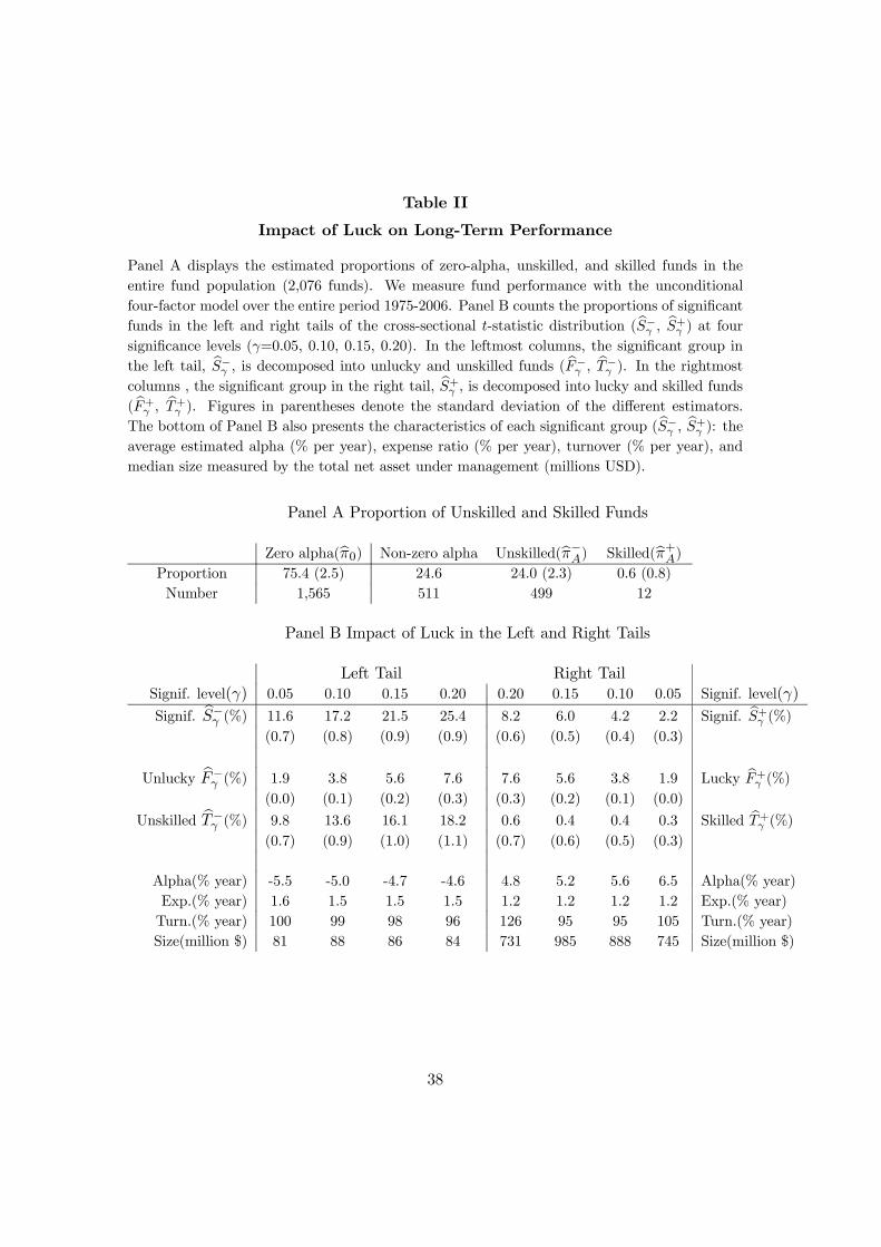
Table II

Impact of Luck on Long-Term Performance

Panel A displays the estimated proportions of zero-alpha, unskilled, and skilled funds in theentire fund population (2,076 funds). We measure fund performance with the unconditionalfour-factor model over the entire period 1975-2006. Panel B counts the proportions of significantfunds in the left and right tails of the cross-sectional t-statistic distribution (bS−γ , bS+γ ) at foursignificance levels (γ=0.05, 0.10, 0.15, 0.20). In the leftmost columns, the significant group inthe left tail, bS−γ , is decomposed into unlucky and unskilled funds ( bF−γ , bT−γ ). In the rightmostcolumns , the significant group in the right tail, bS+γ , is decomposed into lucky and skilled funds( bF+γ , bT+γ ). Figures in parentheses denote the standard deviation of the different estimators.The bottom of Panel B also presents the characteristics of each significant group (bS−γ , bS+γ ): theaverage estimated alpha (% per year), expense ratio (% per year), turnover (% per year), andmedian size measured by the total net asset under management (millions USD).

Panel A Proportion of Unskilled and Skilled Funds

Zero alpha(bπ0) Non-zero alpha Unskilled(bπ−A) Skilled(bπ+A)Proportion 75.4 (2.5) 24.6 24.0 (2.3) 0.6 (0.8)Number 1,565 511 499 12

Panel B Impact of Luck in the Left and Right Tails

Left Tail Right TailSignif. level(γ) 0.05 0.10 0.15 0.20 0.20 0.15 0.10 0.05 Signif. level(γ)

Signif. bS−γ (%) 11.6 17.2 21.5 25.4 8.2 6.0 4.2 2.2 Signif. bS+γ (%)(0.7) (0.8) (0.9) (0.9) (0.6) (0.5) (0.4) (0.3)

Unlucky bF−γ (%) 1.9 3.8 5.6 7.6 7.6 5.6 3.8 1.9 Lucky bF+γ (%)(0.0) (0.1) (0.2) (0.3) (0.3) (0.2) (0.1) (0.0)

Unskilled bT−γ (%) 9.8 13.6 16.1 18.2 0.6 0.4 0.4 0.3 Skilled bT+γ (%)(0.7) (0.9) (1.0) (1.1) (0.7) (0.6) (0.5) (0.3)

Alpha(% year) -5.5 -5.0 -4.7 -4.6 4.8 5.2 5.6 6.5 Alpha(% year)Exp.(% year) 1.6 1.5 1.5 1.5 1.2 1.2 1.2 1.2 Exp.(% year)Turn.(% year) 100 99 98 96 126 95 95 105 Turn.(% year)Size(million $) 81 88 86 84 731 985 888 745 Size(million $)

38

Table III

Impact of Luck on Short-Term Performance

Panel A displays the estimated proportions of zero-alpha, unskilled, and skilled funds in the entirefund population (3,311 funds). We measure fund performance with the unconditional four-factormodel over non-overlapping 5-year periods between 1977-2006. Panel B counts the proportionsof significant funds in the left and right tails of the cross-sectional t-statistic distribution (bS−γ ,bS+γ ) at four significance levels (γ=0.05, 0.10, 0.15, 0.20). In the leftmost columns, the significantgroup in the left tail, bS−γ , is decomposed into unlucky and unskilled funds ( bF−γ , bT−γ ). In therightmost columns , the significant group in the right tail, bS+γ , is decomposed into lucky andskilled funds ( bF+γ , bT+γ ). Figures in parentheses denote the standard deviation of the differentestimators. The bottom of Panel B also presents the characteristics of each significant group(bS−γ , bS+γ ): the average estimated alpha (% per year), expense ratio (% per year), turnover (%per year), and median size measured by the total net asset under management (millions USD).

Panel A Proportion of Unskilled and Skilled Funds

Zero alpha(bπ0) Non-zero alpha Unskilled(bπ−A) Skilled(bπ+A)Proportion 72.2 (2.0) 27.8 25.4 (1.7) 2.4 (0.7)Number 2,390 921 841 80

Panel B Impact of Luck in the Left and Right Tails

Left Tail Right TailSignif. level(γ) 0.05 0.10 0.15 0.20 0.20 0.15 0.10 0.05 Signif. level(γ)

Signif. bS−γ (%) 11.2 16.8 21.4 24.9 9.6 7.8 5.9 3.5 Signif. bS+γ (%)(0.5) (0.6) (0.7) (0.8) (0.5) (0.5) (0.4) (0.3)

Unlucky bF−γ (%) 1.8 3.6 5.4 7.2 7.2 5.4 3.6 1.8 Lucky bF+γ (%)(0.0) (0.0) (0.1) (0.2) (0.2) (0.1) (0.0) (0.0)

Unskilled bT−γ (%) 9.4 13.2 16.0 17.7 2.4 2.4 2.3 1.7 Skilled bT+γ (%)(0.6) (0.7) (0.8) (0.8) (0.6) (0.5) (0.4) (0.3)

Alpha(% year) -6.5 -5.9 -5.5 -5.3 6.7 7.0 7.2 7.5 Alpha(% year)Exp.(% year) 1.4 1.3 1.3 1.3 1.2 1.2 1.2 1.2 Exp.(% year)Turn.(% year) 98 105 100 99 80 81 83 81 Turn.(% year)Size(million $) 242 244 252 244 623 628 664 749 Size(million $)

39

Table IV

Short-Term Performance across Investment Categories

The impact of luck in the left and right tails for three investment categories (Growth, AggressiveGrowth, and Growth & Income funds) is presented in Panels A, B, and C, respectively. Wemeasure fund performance with the unconditional four-factor model over non-overlapping 5-yearperiods between 1977-2006. For each panel, we count the proportions of significant funds inthe left and right tails of the cross-sectional t-statistic distribution (bS−γ , bS+γ ) at four significancelevels (γ=0.05, 0.10, 0.15, 0.20). In the leftmost columns, the significant group in the left tail,bS−γ , is decomposed into unlucky and unskilled funds ( bF−γ , bT−γ ). In the rightmost columns , thesignificant group in the right tail, bS+γ , is decomposed into lucky and skilled funds ( bF+γ , bT+γ ).Figures in parentheses denote the standard deviation of the different estimators. The bottomof Panel B also presents the characteristics of each significant group (bS−γ , bS+γ ): the averageestimated alpha (% per year), expense ratio (% per year), turnover (% per year), and mediansize measured by the total net asset under management (millions USD).

Panel A Growth funds

Left Tail Right TailSignif. level(γ) 0.05 0.10 0.15 0.20 0.20 0.15 0.10 0.05 Signif. level(γ)

Signif. bS−γ (%) 11.3 16.6 21.4 25.2 9.9 8.1 5.9 3.5 Signif. bS+γ (%)(0.7) (0.8) (0.9) (1.0) (0.7) (0.6) (0.5) (0.4)

Unlucky bF−γ (%) 1.8 3.6 5.5 7.3 7.3 5.5 3.6 1.8 Lucky bF+γ (%)(0.0) (0.1) (0.2) (0.2) (0.2) (0.2) (0.1) (0.0)

Unskilled bT−γ (%) 9.5 13.0 15.9 17.9 2.6 2.6 2.3 1.7 Skilled bT+γ (%)(0.7) (0.9) (1.0) (1.1) (0.8) (0.7) (0.6) (0.4)

Alpha(% year) -6.0 -5.6 -5.2 -5.1 6.8 6.8 6.8 7.3 Alpha(% year)Exp.(% year) 1.4 1.3 1.3 1.3 1.2 1.2 1.2 1.2 Exp.(% year)Turn.(% year) 101 113 110 107 79 79 79 75 Turn.(% year)Size(million $) 253 253 253 252 589 593 621 580 Size(million $)

40

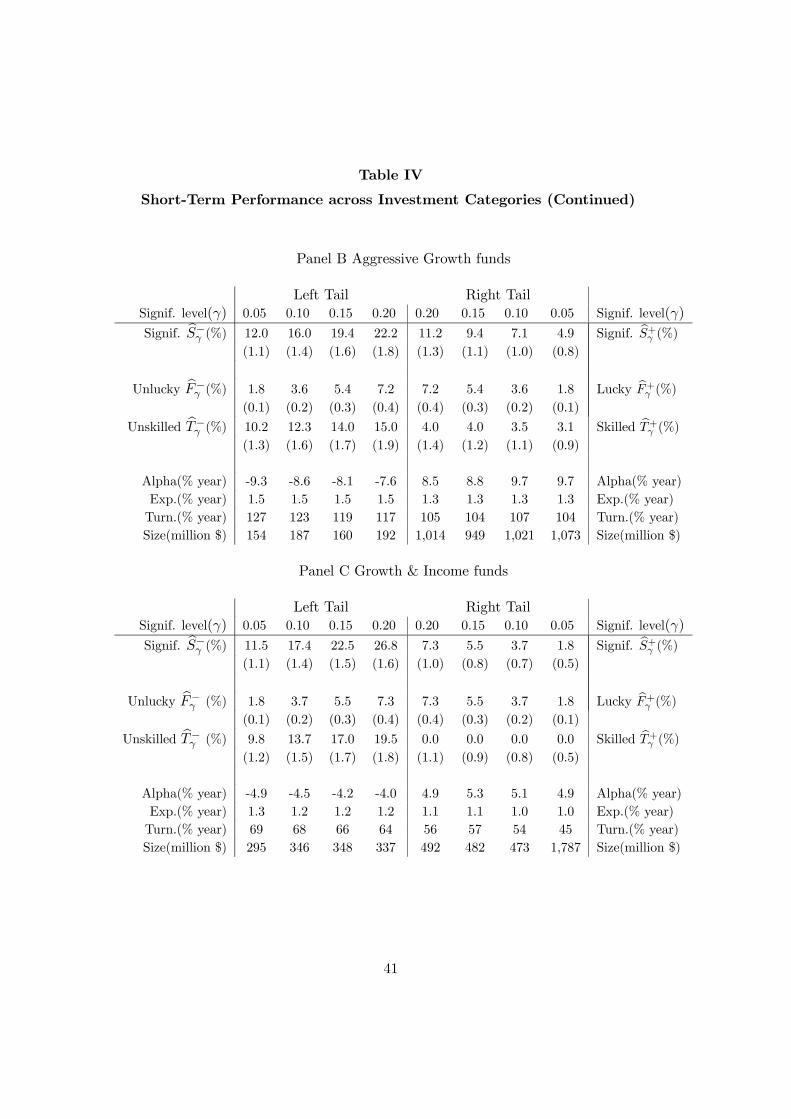
Table IV

Short-Term Performance across Investment Categories (Continued)

Panel B Aggressive Growth funds

Left Tail Right TailSignif. level(γ) 0.05 0.10 0.15 0.20 0.20 0.15 0.10 0.05 Signif. level(γ)

Signif. bS−γ (%) 12.0 16.0 19.4 22.2 11.2 9.4 7.1 4.9 Signif. bS+γ (%)(1.1) (1.4) (1.6) (1.8) (1.3) (1.1) (1.0) (0.8)

Unlucky bF−γ (%) 1.8 3.6 5.4 7.2 7.2 5.4 3.6 1.8 Lucky bF+γ (%)(0.1) (0.2) (0.3) (0.4) (0.4) (0.3) (0.2) (0.1)

Unskilled bT−γ (%) 10.2 12.3 14.0 15.0 4.0 4.0 3.5 3.1 Skilled bT+γ (%)(1.3) (1.6) (1.7) (1.9) (1.4) (1.2) (1.1) (0.9)

Alpha(% year) -9.3 -8.6 -8.1 -7.6 8.5 8.8 9.7 9.7 Alpha(% year)Exp.(% year) 1.5 1.5 1.5 1.5 1.3 1.3 1.3 1.3 Exp.(% year)Turn.(% year) 127 123 119 117 105 104 107 104 Turn.(% year)Size(million $) 154 187 160 192 1,014 949 1,021 1,073 Size(million $)

Panel C Growth & Income funds

Left Tail Right TailSignif. level(γ) 0.05 0.10 0.15 0.20 0.20 0.15 0.10 0.05 Signif. level(γ)

Signif. bS−γ (%) 11.5 17.4 22.5 26.8 7.3 5.5 3.7 1.8 Signif. bS+γ (%)(1.1) (1.4) (1.5) (1.6) (1.0) (0.8) (0.7) (0.5)

Unlucky bF−γ (%) 1.8 3.7 5.5 7.3 7.3 5.5 3.7 1.8 Lucky bF+γ (%)(0.1) (0.2) (0.3) (0.4) (0.4) (0.3) (0.2) (0.1)

Unskilled bT−γ (%) 9.8 13.7 17.0 19.5 0.0 0.0 0.0 0.0 Skilled bT+γ (%)(1.2) (1.5) (1.7) (1.8) (1.1) (0.9) (0.8) (0.5)

Alpha(% year) -4.9 -4.5 -4.2 -4.0 4.9 5.3 5.1 4.9 Alpha(% year)Exp.(% year) 1.3 1.2 1.2 1.2 1.1 1.1 1.0 1.0 Exp.(% year)Turn.(% year) 69 68 66 64 56 57 54 45 Turn.(% year)Size(million $) 295 346 348 337 492 482 473 1,787 Size(million $)

41

Table V

Performance Persistence Based on the False Discovery Rate

For each of the five FDR targets (10%, 30%, 50%, 70%, and 90%), Panel A contains descriptive

statistics on the FDR level (\FDR+

γP ) achieved by each portfolio, as well as the proportion of

funds in the population that it includes (bS+γP). The panel shows the average values of \FDR

+

γP

and bS+γP

over the 27 annual formation dates (from December 1979 to 2005), as well as theirrespective distributions. Panel B displays the performance of each portfolio over the period1980-2006. We estimate the annual four-factor alpha (bα) with its bootstrap p-value, its annualresidual standard deviation (bσε), its annual information ratio (IR=bα/bσε), its loadings on themarket (bbm), size (bbsmb), book-to-market (bbhml), and momentum factors (bbmom), and its annualexcess mean, and standard deviation. In Panel C, we examine the turnover of each portfolio.We compute the proportion of funds that are still included in the portfolio 1, 2, 3, 4, and 5 yearsafter their initial selection.

Panel A Portfolio Statistics

Achieved False Discovery Rate³\FDR

+

γP

´Included proportion of funds(bS+

γP)

Mean 10-30 30-50 50-70 >70% Mean 0-6 6-12 12-24 >24%FDR10% 41.5% 14 6 1 6 3.0% 25 2 0 0FDR30% 47.5% 8 12 1 6 8.2% 15 7 3 2FDR50% 60.4% 0 14 7 6 20.9% 5 7 4 11FDR70% 71.3% 0 4 12 11 29.7% 1 5 5 16FDR90% 75.0% 0 4 9 14 33.7% 0 3 4 20

Panel B Performance Analysis

bα(p-value) bσε IR bbm bbsmbbbhml

bbmom Mean Std devFDR10% 1.45%(0.04) 4.0% 0.36 0.93 0.16 -0.04 -0.02 8.3% 15.4%FDR30% 1.15%(0.05) 3.3% 0.35 0.94 0.17 -0.02 -0.03 8.1% 15.4%FDR50% 0.95%(0.10) 2.9% 0.33 0.96 0.20 -0.06 -0.01 8.1% 16.1%FDR70% 0.68%(0.15) 2.7% 0.25 0.97 0.19 -0.06 -0.01 7.9% 16.1%FDR90% 0.39%(0.30) 2.7% 0.14 0.97 0.19 -0.05 -0.00 7.8% 16.0%

Panel C Portfolio Turnover

Proportion of funds remaining in the portfolio...After 1 year After 2 years After 3 years After 4 years After 5 years

FDR10% 36.7 12.8 3.4 0.8 0.0FDR30% 40.0 14.7 5.1 1.7 1.3FDR50% 48.8 23.5 12.3 4.7 2.6FDR70% 52.2 29.0 17.4 9.5 6.3FDR90% 55.9 33.8 20.4 13.0 8.5

42

Table VI

Impact of Luck on Long-Term Pre-Expense Performance

Panel A displays the estimated proportions of zero-alpha, unskilled, and skilled funds in theentire fund population on a pre-expense basis (1,836 funds). We add the monthly expensesto net return of each fund, and measure performance with the unconditional four-factor modelover the entire period 1975-2006. Panel B counts the proportions of significant funds in theleft and right tails of the cross-sectional t-statistic distribution (bS−γ , bS+γ ) at four significancelevels (γ=0.05, 0.10, 0.15, 0.20). In the leftmost columns, the significant group in the left tail,bS−γ , is decomposed into unlucky and unskilled funds ( bF−γ , bT−γ ). In the rightmost columns , thesignificant group in the right tail, bS+γ , is decomposed into lucky and skilled funds ( bF+γ , bT+γ ).Figures in parentheses denote the standard deviation of the different estimators. The bottomof Panel B also presents the characteristics of each significant group (bS−γ , bS+γ ): the averageestimated alpha prior to expenses (in % per year), expense ratio (in % per year), turnover (in% per year), and median size measured by the total net asset under management (in millions ofdollars).

Panel A Proportion of Unskilled and Skilled Funds

Zero alpha(bπ0) Non-zero alpha Unskilled(bπ−A) Skilled(bπ+A)Proportion 85.9 (2.7) 14.1 4.5 (1.0) 9.6 (1.5)Number 1,577 259 176 83

Panel B Impact of Luck in the Left and Right Tails

Left Tail Right TailSignif. level(γ) 0.05 0.10 0.15 0.20 0.20 0.15 0.10 0.05 Signif. level(γ)

Signif. bS−γ (%) 4.3 7.5 10.2 12.8 17.3 13.1 9.3 5.8 Signif. bS+γ (%)(0.5) (0.6) (0.7) (0.8) (0.9) (0.8) (0.7) (0.5)

Unlucky bF−γ (%) 2.1 4.3 6.4 8.6 8.6 6.4 4.3 2.1 Lucky bF+γ (%)(0.0) (0.1) (0.1) (0.2) (0.2) (0.1) (0.1) (0.0)

Unskilled bT−γ (%) 2.2 3.2 3.8 4.2 8.7 6.6 5.0 3.6 Skilled bT+γ (%)(0.5) (0.6) (0.8) (0.9) (1.0) (0.9) (0.7) (0.5)

Pre Expense Pre ExpenseAlpha(% year) -5.9 -5.2 -4.8 -4.5 4.4 4.8 5.0 5.3 Alpha(% year)Exp.(% year) 1.5 1.4 1.3 1.3 1.3 1.3 1.3 1.3 Exp.(% year)Turn.(% year) 105 108 108 108 106 111 122 84 Turn.(% year)Size(million $) 81 90 93 90 430 578 948 1,000 Size(million $)

43

Table VII

Loadings on Omitted Factors

We determine the proportions of significant funds in the left and right tails (bS−γ , bS+γ ) at foursignificance levels (γ=0.05, 0.10, 0.15, 0.20) according to each asset-pricing model over the period1975-2006. For each of these significant groups, we compute their average loadings on the omittedfactors from the four-factor model: size (bbsmb), book-to-market (bbhml), and momentum (bbmom).Panel A shows the results obtained with the unconditional CAPM, while Panel B repeats thesame procedure with the unconditional Fama-French model.

Panel A Unconditional CAPM

Left Tail Right TailSignif. level(γ) 0.05 0.10 0.15 0.20 0.20 0.15 0.10 0.05 Signif. level(γ)

Size(bbsmb) 0.06 0.07 0.09 0.09 0.27 0.28 0.28 0.36 Size(bbsmb)

Book(bbhml) -0.14 -0.14 -0.13 -0.14 0.34 0.35 0.36 0.37 Book(bbhml)

Mom.(bbmom) 0.00 0.00 0.00 0.01 -0.01 -0.01 -0.02 -0.01 Mom.(bbmom)

Panel B Unconditional Fama-French model

Left Tail Right TailSignif. level(γ) 0.05 0.10 0.15 0.20 0.20 0.15 0.10 0.05 Signif. level(γ)

Mom.(bbmom) -0.02 -0.03 -0.02 -0.03 0.09 0.10 0.11 0.12 Mom.(bbmom)

44

Figure 1

Outcome of the Multiple Performance Test

Panel A shows the distribution of the fund t-statistic across the three skill groups (zero-alpha, unskilled, and skilled funds). We set the true four-factor alpha equal to -3.2%and +3.8% per year for the unskilled and skilled funds (implying that the t-statistic dis-tributions are centered at -2.5 and +3). Panel B displays the cross-sectional t-statisticdistribution. It is a mixture of the three distributions in Panel A, where the weight oneach distribution depends on the proportion of zero-alpha, unskilled, and skilled fundsin the population (π0, π−A, and π+A). In this example, we set π0 = 75%, π−A = 23%,and π+A = 2% to match our average estimated values over the final 5 years of our sample.

-5.5 -5 -4.5 -4 -3.5 -3 -2.5 -2 -1.5 -1 -0.5 0 0.5 1 1.5 2 2.5 3 3.5 4 4.5 5 5.5 60

0.1

0.2

0.3

0.4

0.5

t-statistic

dens

ity

-5.5 -5 -4.5 -4 -3.5 -3 -2.5 -2 -1.5 -1 -0.5 0 0.5 1 1.5 2 2.5 3 3.5 4 4.5 5 5.5 60

0.1

0.2

0.3

0.4

0.5

t-statistic

dens

ity

PANEL A: INDIVIDUAL FUND T-STATISTIC DISTRIBUTION

PANEL B: CROSS-SECTIONAL T-STATISTIC DISTRIBUTION

UNSKILLED FUNDSmean t=-2.5

ZERO-ALPHA FUNDSmean t=0

SKILLED FUNDSmean t=3.0

Probability of being unlucky

Probability of being lucky

Threshold= -1.65 Threshold=+1.65

PROPORTION OFUNSKILLED FUNDS=23%

PROPORTION OF ZERO-ALPHA FUNDS=75%

PROPORTION OF SKILLED FUNDS=2%

The proportion of significant funds is equal to 20.3%

But are all these funds truly unskilled?The proportion of significant fundsis equal to 5.4%

But are all these funds truly skilled?

45

Figure 2

Histogram of Fund p-values

This figure represents the p-value histogram of M=2,076 funds (as in our database). Foreach fund, we draw its t-statistic from one of the distributions in Figure 1 (Panel A)according to the proportion of zero-alpha, unskilled, and skilled funds in the population(π0, π−A, and π+A). In this example, we set π0 = 75%, π−A = 23%, and π+A = 2% tomatch our average estimated values over the final 5 years of our sample. Then, we computethe two-sided p-values of each fund from its respective t-statistic, and plot them in the histogram.

0 0.1 0.2 0.3 0.4 0.5 0.6 0.7 0.8 0.9 10

0.05

0.1

0.15

0.2

0.25

0.3

estimated p-values

dens

ity

0 0.1 0.2 0.3 0.4 0.5 0.6 0.7 0.8 0.9 10 0.1 0.2 0.3 0.4 0.5 0.6 0.7 0.8 0.9 1

p-values of the unskilledand skilled funds

Area containing the p-values ofthe zero-alpha funds

Proportion of funds represented bythese four rectangles=W( λ*)/M,where W( λ*)=number(p-values> λ*)

λ*

The area below this line equals the (unknown)proportion of zero-alpha funds, π

0(which we must estimate from the p-values)

46

Figure 3

Measuring Luck: Comparison with Existing Approaches

This figure examines the bias of different estimators produced by the three approaches ("noluck", "full luck", and "our approach") as a function of the proportion of zero-alpha funds, π0.We examine the estimators of the proportions of unlucky, lucky, unskilled, and skilled funds inPanel A, B, C, and D, respectively. The "no luck" approach assumes that π0=0, the "full luck"approach assumes that π0=1, while "our approach" estimates π0 directly from the data. Foreach approach, we compare the average estimator value (over 1,000 replications) with the truepopulation value. For each replication, we draw the t-statistic for each fund i (i=1,...,2,076)from one of the distributions in Figure 1 (Panel A) according to the weights π0, π

−A, and π+A,

and compute the different estimators at the significance level γ = 0.20. For each π0, the ratioπ−A over π

+A is held fixed to 11.5 (0.23/0.02) as in Figure 1.

0 0.1 0.2 0.3 0.4 0.5 0.6 0.7 0.8 0.9 1

0

0.01

0.02

0.03

0.04

0.05

0.06

0.07

0.08

0.09

0.1

proportion of zero-alpha funds ( π0)

estim

ated

pro

porti

on o

f unl

ucky

fund

s (a

vera

ge)

Full luck approach

(bias increases as π0 goes to one)

Our approach

True value

(bias increases as π0 goes to zero)

No luck approach

(A) Unlucky funds (left tail)

0 0.1 0.2 0.3 0.4 0.5 0.6 0.7 0.8 0.9 1

0

0.01

0.02

0.03

0.04

0.05

0.06

0.07

0.08

0.09

0.1

proportion of zero-alpha funds ( π0)

estim

ated

pro

porti

on o

f luc

ky fu

nds

(ave

rage

)

Full luck approach

No luck approach

Our approach

True value

(B) Lucky funds (right tail)

0 0.1 0.2 0.3 0.4 0.5 0.6 0.7 0.8 0.9 10

0.1

0.2

0.3

0.4

0.5

0.6

0.7

0.8

proportion of zero-alpha funds ( π0)

estim

ated

pro

porti

on o

f uns

kille

d fu

nds

(ave

rage

)

No luck approach

Our approach & True value

Full luck approach

(the two lines are the same)

(C) Unskilled funds (left tail)

0 0.1 0.2 0.3 0.4 0.5 0.6 0.7 0.8 0.9 1

-0.02

-0.01

0

0.01

0.02

0.03

0.04

0.05

0.06

0.07

0.08

0.09

0.1

proportion of zero-alpha funds ( π0)

estim

ated

pro

porti

on o

f ski

lled

fund

s (a

vera

ge)

No luck approach

True value

Our approach

(wrongly rises with π0wrongly produces negative estimates)

(wrongly rises with π0)

Full luck approach

(D) Skilled funds (right tail)

47

Figure 4

Evolution of Mutual Fund Performance over Time

Panel A plots the evolution of the estimated proportions of unskilled and skilled funds(bπ−A and bπ+A) between 1989 and 2006. At the end of each year, we measure bπ−A and bπ+Ausing the entire fund return history up to that point. The initial estimates at the endof 1989 cover the period 1975-1989, while the last ones in 2006 use the period 1975-2006.The performance of each fund is measured with the unconditional four-factor model.Panel B displays the growth in the mutual fund industry (proxied by the total number offunds used to compute bπ−A and bπ+A over time), as well as its average alpha (in % per year).

1989 1990 1991 1992 1993 1994 1995 1996 1997 1998 1999 2000 2001 2002 2003 2004 2005 20060

5

10

15

20

25

30

35

End of the year

Prop

ortio

n of

fund

s (in

per

cent

)

1989 1990 1991 1992 1993 1994 1995 1996 1997 1998 1999 2000 2001 2002 2003 2004 2005 20060

200400600800

1000120014001600180020002200

Tota

l num

ber o

f fun

ds

End of the year

-1

-0.75

-0.5

-0.25

0

0.25

0.5

Annu

al a

vera

ge a

lpha

(in

perc

ent)

Number of funds

Average alpha

Unskilled & Skilled funds

Unskilled funds

Skilled funds

PANEL A: PROPORTIONS OF UNSKILLED AND SKILLED FUNDS

PANEL B: TOTAL NUMBER OF FUNDS AND AVERAGE ALPHA

48

Figure 5

Performance of the Portfolios FDR10% over Time

The graph plots the evolution of the estimated annual four-factor alpha of the portfolioFDR10%. This portfolio contains funds located in the right tail of the cross-sectional t-statisticdistribution such that the targeted proportion of lucky funds included in the portfolio isequal to 10%. At the end of each year from 1989 to 2006, the portfolio’s alpha is estimatedusing the portfolio return history up to that point. The initial estimates cover the period1980-1989 (the first five years are used for the initial portfolio formation on December 31,1979), while the last ones use the entire portfolio history from 1980 up to 2006. For comparisonpurposes, we also show the performance of top decile portfolios formed according to a t-statisticranking, where the t-statistic is estimated over the prior one and three years, respectively.

1989 1990 1991 1992 1993 1994 1995 1996 1997 1998 1999 2000 2001 2002 2003 2004 2005 20060

0.250.5

0.751

1.251.5

1.752

2.252.5

2.753

3.253.5

3.754

4.254.5

4.755

End of the year

Ann

ual a

lpha

(in

perc

ent)

FDR10%

Top Decile t-statistic (1 year ranking)

Top Decile t-statistic (3 years ranking)

49