Fall 2017

MA 16100

Study Guide - Final Exam

1 Review of Algebra/PreCalculus:

(a) Distance between P (x1, y1) and P (x2, y2) is |PQ| =√

(x2 − x1)2 + (y2 − y1)2.(b) Equations of lines:

(i) Point-Slope Form: y − y1 = m(x− x1)(ii) Slope-Intercept Form: y = mx+ b

(c) L1||L2 ⇐⇒ m1 = m2 ; L1 ⊥ L2 ⇐⇒ m2 = − 1

m1

(d) Equation of a circle: (x− h)2 + (y − k)2 = r2.

(e) Determining domain of a function f(x).

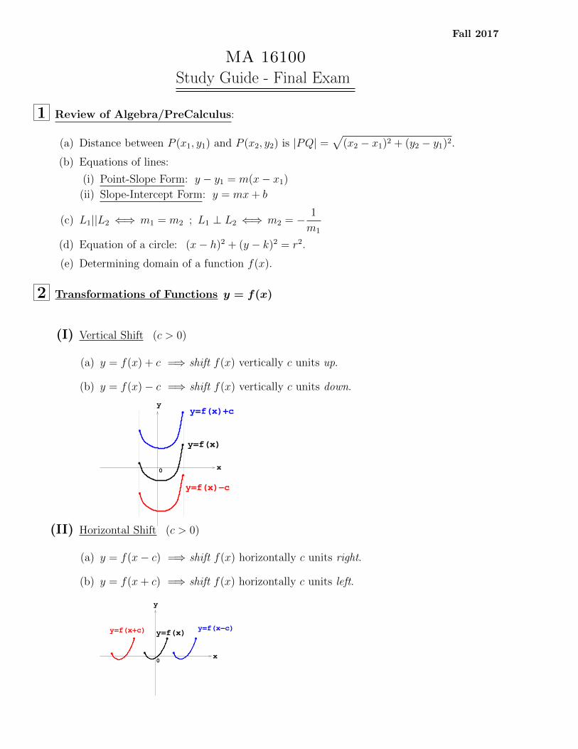
2 Transformations of Functions y = f(x)

(I) Vertical Shift (c > 0)

(a) y = f(x) + c =⇒ shift f(x) vertically c units up.

(b) y = f(x)− c =⇒ shift f(x) vertically c units down.

yy=f(x)+c

y=f(x)−c

0 x

y=f(x)

(II) Horizontal Shift (c > 0)

(a) y = f(x− c) =⇒ shift f(x) horizontally c units right.

(b) y = f(x+ c) =⇒ shift f(x) horizontally c units left.

x

y

0

y=f(x)y=f(x+c) y=f(x−c)

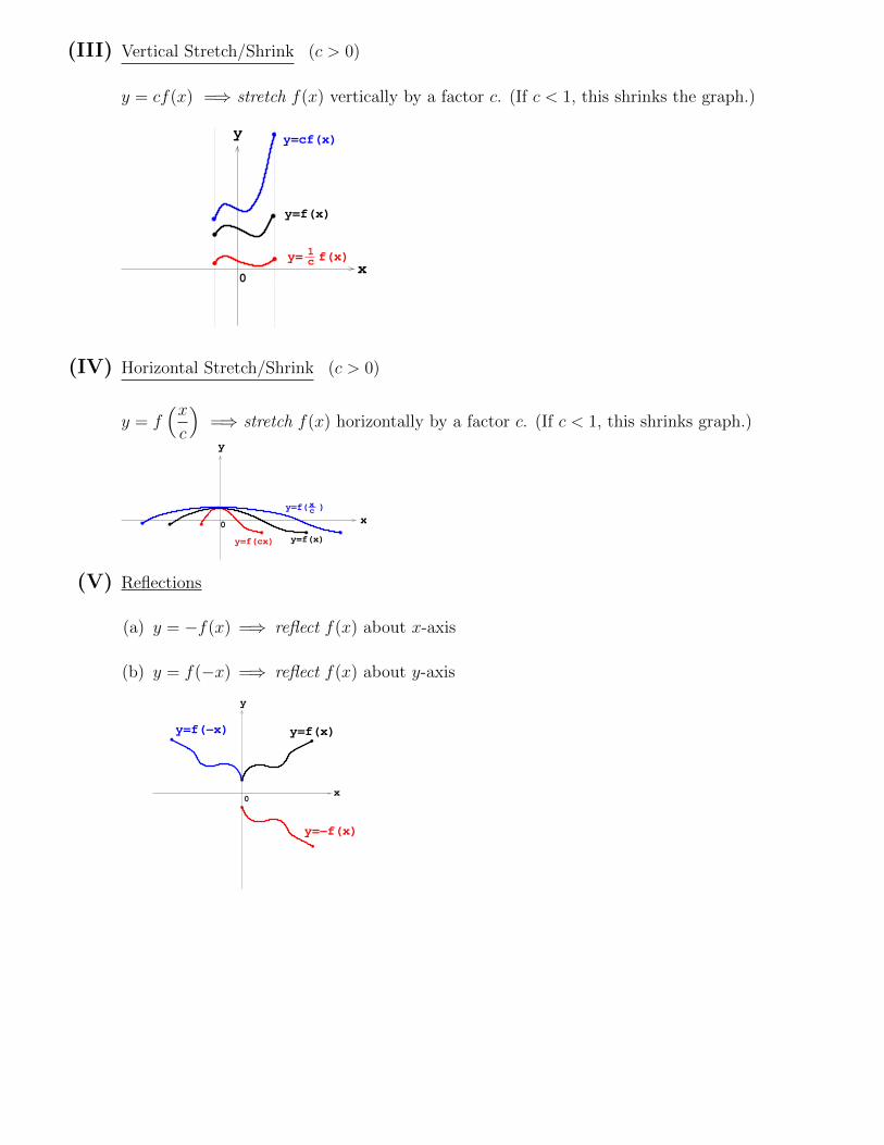
(III) Vertical Stretch/Shrink (c > 0)

y = cf(x) =⇒ stretch f(x) vertically by a factor c. (If c < 1, this shrinks the graph.)

x0

y=cf(x)

y= f(x)1c

y=f(x)

y

(IV) Horizontal Stretch/Shrink (c > 0)

y = f(xc

)=⇒ stretch f(x) horizontally by a factor c. (If c < 1, this shrinks graph.)

y=f(x)

y=f( )

0

y

x

y=f(cx)

xc

(V) Reflections

(a) y = −f(x) =⇒ reflect f(x) about x-axis

(b) y = f(−x) =⇒ reflect f(x) about y-axis

y

0x

y=f(x)y=f(−x)

y=−f(x)

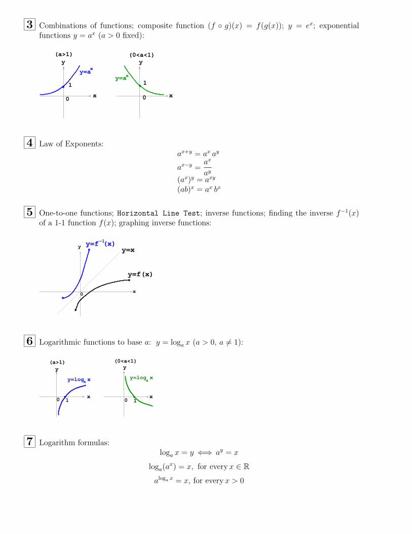
3 Combinations of functions; composite function (f ◦ g)(x) = f(g(x)); y = ex; exponentialfunctions y = ax (a > 0 fixed):

0

1

0

1

y=ay=ax

x

(a>1)y

x

y

x

(0<a<1)

4 Law of Exponents:ax+y = ax ay

ax−y =ax

ay(ax)y = axy

(ab)x = ax bx

5 One-to-one functions; Horizontal Line Test; inverse functions; finding the inverse f−1(x)of a 1-1 function f(x); graphing inverse functions:

y

x0

y=xy=f (x)−1

y=f(x)

6 Logarithmic functions to base a: y = loga x (a > 0, a 6= 1):

y

x

(0<a<1)

x

y(a>1)

y=log xa

0 1 0 1

y=log xa

7 Logarithm formulas:loga x = y ⇐⇒ ay = x

loga(ax) = x, for every x ∈ R

aloga x = x, for every x > 0

8 Law of Logarithms: loga(xy) = loga x+ loga y

loga

(x

y

)= loga x− loga y

loga(xp) = p loga x

9 Finite Limits

(a) limx→a

f(x) = L

y

x0

L

a

y=f(x)

(b) limx→a+

f(x) = L (right-hand limit)

y

x0

L

y=f(x)

a

(c) limx→a−

f(x) = L (left-hand limit)

y

x0

L

y=f(x)

a

Recall: limx→a

f(x) = L ⇐⇒ limx→a+

f(x) = limx→a−

f(x) = L

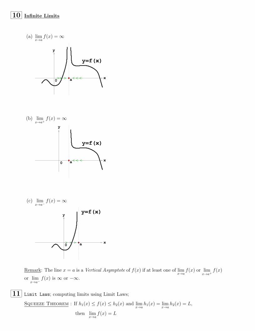
10 Infinite Limits

(a) limx→a

f(x) =∞

x0

y

y=f(x)

a

(b) limx→a+

f(x) =∞

xa

y=f(x)

0

y

(c) limx→a−

f(x) =∞

0 a

yy=f(x)

x

Remark: The line x = a is a Vertical Asymptote of f(x) if at least one of limx→a

f(x) or limx→a+

f(x)

or limx→a−

f(x) is ∞ or −∞.

11 Limit Laws; computing limits using Limit Laws;

Squeeze Theorem : If h1(x) ≤ f(x) ≤ h2(x) and limx→a

h1(x) = limx→a

h2(x) = L,

then limx→a

f(x) = L

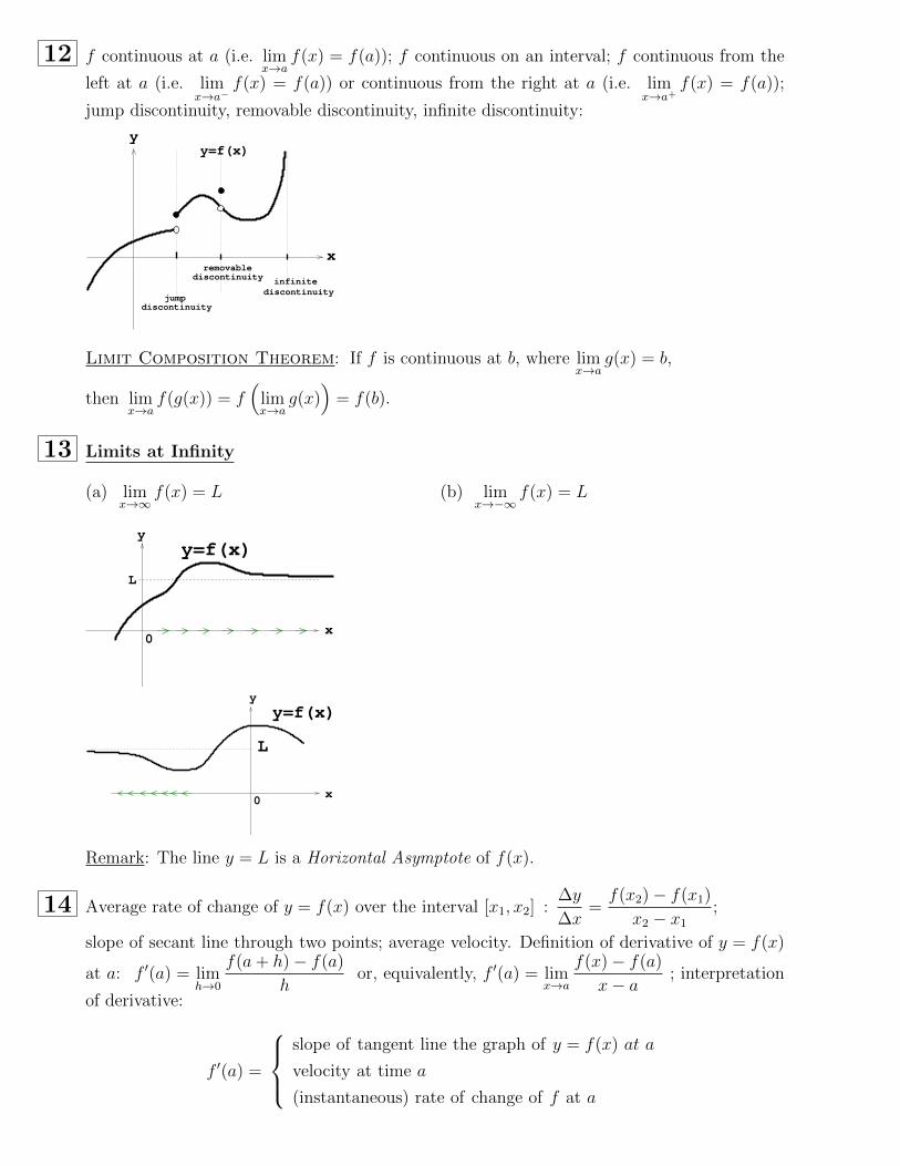
12 f continuous at a (i.e. limx→a

f(x) = f(a)); f continuous on an interval; f continuous from the

left at a (i.e. limx→a−

f(x) = f(a)) or continuous from the right at a (i.e. limx→a+

f(x) = f(a));

jump discontinuity, removable discontinuity, infinite discontinuity:

infinite

removable

jumpdiscontinuity

discontinuity

discontinuity

y

x

y=f(x)

Limit Composition Theorem: If f is continuous at b, where limx→a

g(x) = b,

then limx→a

f(g(x)) = f(

limx→a

g(x))

= f(b).

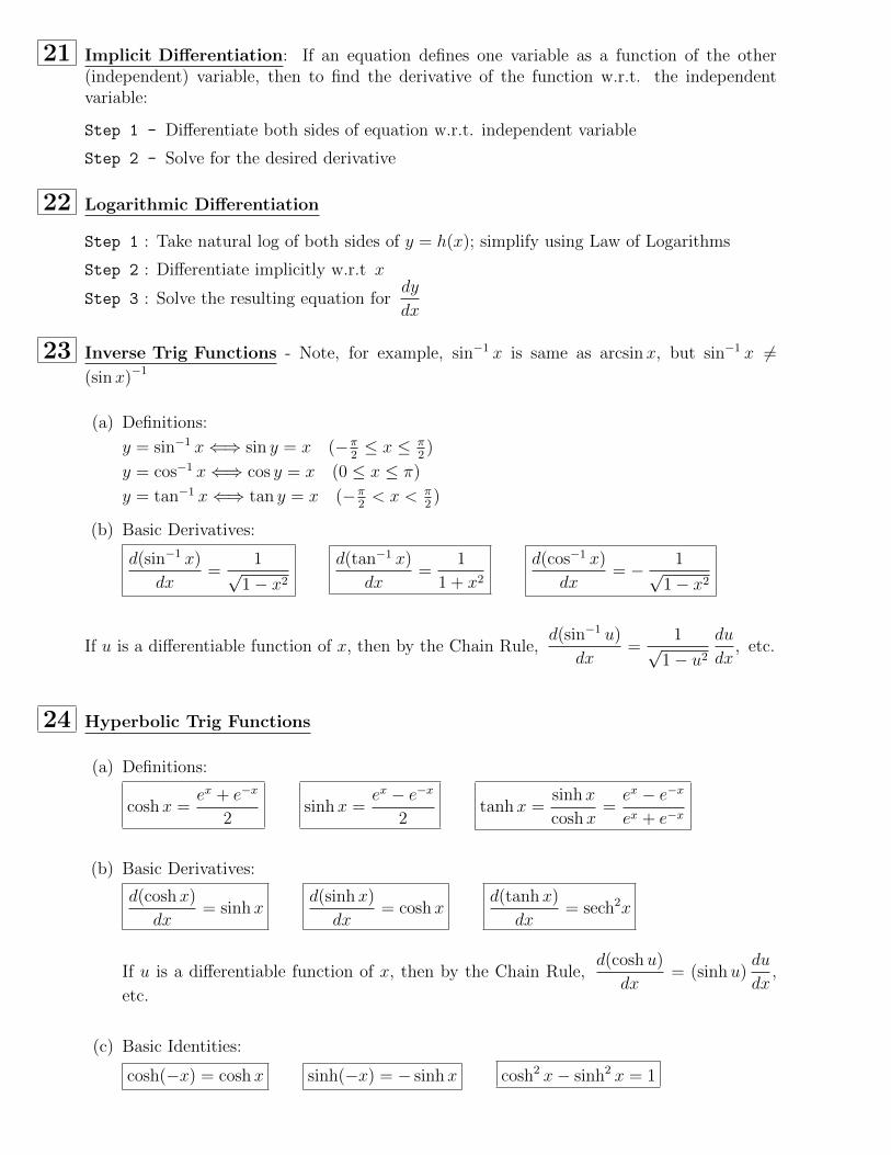
13 Limits at Infinity

(a) limx→∞

f(x) = L (b) limx→−∞

f(x) = L

0

yy=f(x)

x

L

0x

L

y

y=f(x)

Remark: The line y = L is a Horizontal Asymptote of f(x).

14 Average rate of change of y = f(x) over the interval [x1, x2] :∆y

∆x=f(x2)− f(x1)

x2 − x1;

slope of secant line through two points; average velocity. Definition of derivative of y = f(x)

at a: f ′(a) = limh→0

f(a+ h)− f(a)

hor, equivalently, f ′(a) = lim

x→a

f(x)− f(a)

x− a; interpretation

of derivative:

f ′(a) =

slope of tangent line the graph of y = f(x) at a

velocity at time a

(instantaneous) rate of change of f at a

15 Derivative as a function: f ′(x) = limh→0

f(x+ h)− f(x)

h=

dy

dx; differentiable functions (i.e.,

f ′(x) exists); higher order derivatives : f ′′(x) =d2y

dx2, . . . .

16 Average rate of change of y = f(x) over the interval [x1, x2] :∆y

∆x=f(x2)− f(x1)

x2 − x1(this is also

the average velocity). Definition of derivative of y = f(x) at a: f ′(a) = limh→0

f(a+ h)− f(a)

h

or, equivalently, f ′(a) = limx→a

f(x)− f(a)

x− a; interpretation of derivative:

f ′(a) =

slope of tangent line the graph of y = f(x) at a

velocity at time a

(instantaneous) rate of change of f at a

17 Derivative as a function: f ′(x) = limh→0

f(x+ h)− f(x)

h; differentiable functions (i.e., f ′(x)

exists);

higher order derivatives: y′′ or equivalentlyd2y

dx2; y′′′ or equivalently

d3y

dx3; etc...

18 Basic Differentiation Rules: If f and g are differentiable functions, and c is a constant:

(a)d(c)

dx= 0 (b)

d(u+ v)

dx=du

dx+dv

dx(c)

d(u− v)

dx=du

dx− dv

dx

(c) Power Rule:d(xn)

dx= nxn−1

(d) Product Rule :d(uv)

dx= u

dv

dx+ v

du

dxQuotient Rule :

d(uv

)dx

=vdu

dx− u dv

dxv2

19 Special Trig Limits : limθ→ 0

sin θ

θ= 1 lim

θ→ 0

θ

sin θ= 1 lim

θ→ 0

cos θ − 1

θ= 0 .

Hence also limθ→ 0

sin(kθ)

(kθ)= 1 and lim

θ→ 0

(kθ)

sin(kθ)= 1. Note that sin kθ 6= k sin θ.

20 CHAIN RULE: If g is differentiable at x and f is differentiable at g(x), then the compositefunction f ◦ g is differentiable at x and its derivative is

(f ◦ g)′(x) =

{f(g(x))

}′= f ′(g(x)) g′(x)

i.e., if y = f(u) and u = g(x), thendy

dx=dy

du

du

dx.

21 Implicit Differentiation: If an equation defines one variable as a function of the other(independent) variable, then to find the derivative of the function w.r.t. the independentvariable:

Step 1 - Differentiate both sides of equation w.r.t. independent variable

Step 2 - Solve for the desired derivative

22 Logarithmic Differentiation

Step 1 : Take natural log of both sides of y = h(x); simplify using Law of Logarithms

Step 2 : Differentiate implicitly w.r.t x

Step 3 : Solve the resulting equation fordy

dx

23 Inverse Trig Functions - Note, for example, sin−1 x is same as arcsinx, but sin−1 x 6=(sinx)−1

(a) Definitions:

y = sin−1 x⇐⇒ sin y = x (−π2≤ x ≤ π

2)

y = cos−1 x⇐⇒ cos y = x (0 ≤ x ≤ π)

y = tan−1 x⇐⇒ tan y = x (−π2< x < π

2)

(b) Basic Derivatives:

d(sin−1 x)

dx=

1√1− x2

d(tan−1 x)

dx=

1

1 + x2d(cos−1 x)

dx= − 1√

1− x2

If u is a differentiable function of x, then by the Chain Rule,d(sin−1 u)

dx=

1√1− u2

du

dx, etc.

24 Hyperbolic Trig Functions

(a) Definitions:

coshx =ex + e−x

2sinhx =

ex − e−x

2tanhx =

sinhx

coshx=ex − e−x

ex + e−x

(b) Basic Derivatives:

d(coshx)

dx= sinhx

d(sinhx)

dx= coshx

d(tanhx)

dx= sech2x

If u is a differentiable function of x, then by the Chain Rule,d(coshu)

dx= (sinhu)

du

dx,

etc.

(c) Basic Identities:

cosh(−x) = cosh x sinh(−x) = − sinhx cosh2 x− sinh2 x = 1

25 APPLICATIONS

Model 1 - Exponential Growth/Decay:dy

dt= k y where k = relative growth/decay

rate

(If the rate of change of y is proportional to y, then the above differential equation holds.)

• If k > 0, this is the law of Natural Growth (for example, population growth).

• If k < 0, this is the law of Natural Decay (for example, radioactive decay).

All solutions to this differential equation have the form y(t) = y(0) ekt .

(Usually need two pieces of information to determine both constants y(0) and k, unlessthey are given explicitly.)

Half-life = time it takes for radioactive substance to lose half its mass.)

Model 2 - Newton’s Law of Cooling : If T (t) = temperature of an object at time t and

Ts = temperature of its surrounding environment, then the rate of change of T (t) isproportional to the difference between T (t) and Ts :

dT

dt= k (T (t)− Ts)

The solution to this particular differential equation is always T (t) = Ts + Cekt

(Usually need two pieces of information to determine both constants C and k, unlessthey are given explicitly.)

Model 3 - Related Rates (Method to Solve) :

1 Read problem carefully several times to understand what is asked.

2 Draw a picture (if possible) and label.

3 Write down the given rate; write down the desired rate.

4 Find an equation relating the variables.

5 Use Chain Rule to differentiate equation w.r.t to time and solve for desired rate.

Useful Formulas for Related Rates

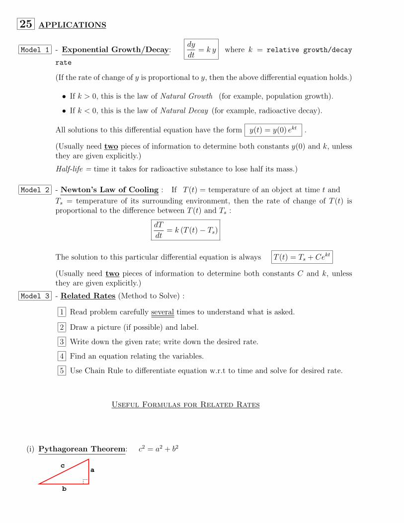
(i) Pythagorean Theorem: c2 = a2 + b2

ca

b

(ii) Similar Triangles:a

b=A

B

B

A

b

a

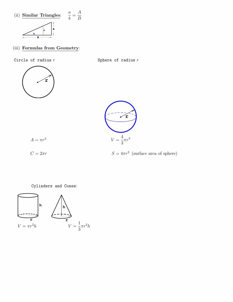
(iii) Formulas from Geometry:

Circle of radius r Sphere of radius r

r

r

A = πr2 V =4

3πr3

C = 2πr S = 4πr2 (surface area of sphere)

Cylinders and Cones:

r

h h

r

V = πr2h V =1

3πr2h

Additional Differentiation Formulas(u is a differentiable function of x)

d (un)

dx= nun−1

du

dx

d (eu)

dx= eu

du

dx

d (au)

dx= au (ln a)

du

dx

d (lnu)

dx=

1

u

du

dx

d (loga u)

dx=

1

u ln a

du

dx

d (sinu)

dx= (cosu)

du

dx

d (cosu)

dx= (− sinu)

du

dx

d (tanu)

dx= (sec2 u)

du

dx

d (cscu)

dx= (− cscu cotu)

du

dx

d (secu)

dx= (secu tanu)

du

dx

d (cotu)

dx= (− csc2 u)

du

dx

26 Related Rates Word Problems Method:

1 Read problem carefully several times to understand what is asked.

2 Draw a picture (if possible) and label.

3 Write down the given rate; write down the desired rate.

4 Find an equation relating the variables.

5 Use Chain Rule to differentiate equation w.r.t to time and solve for desired rate.

27 The Linear Approximation (or tangent line approximation) to a function f(x) at x = a is the

function L(x) = f(a) + f ′(a)(x−a); Approximation formula f(x) ≈ f(a) + f ′(a)(x− a) for

x near a; if y = f(x), the differential of y is dy = f ′(x)dx.

28 Definitions of absolute maximum, absolute minimum, local/relative maxmium, and local/relativeminimum; c is a critical number of f if c is in the domain of f and either f ′(c) = 0 or f ′(c)DNE.

29 Extreme Value Theorem: If f(x) is continuous on a closed interval [a, b], then f alwayshas an absolute maximum value and an absolute minimum value on [a, b].

30 Method to Find Absolute Max/Min of f(x) over Closed Interval [a, b]:

(i) Find all admissible critical numbers in (a, b);

(ii) Find endpoints of interval;

(iii) Make table of values of f(x) at the points found in (i) and (ii).

The largest value = abs max value of f and the smallest value = abs min value of f .

31 Rolle’s Theorem: If f(x) is continuous on [a, b] and differentiable on (a, b), and f(a) = f(b),then f ′(c) = 0 for some c ∈ (a, b).

32 Mean Value Theorem: If f(x) is continuous on [a, b] and differentiable on (a, b), then there

is a number c, where a < c < b, such thatf(b)− f(a)

b− a= f ′(c) :

i.e., f(b)− f(a) = f ′(c) (b− a)

If something about f ′ is known, then something about the sizes of f(a) and f(b) can be found.

33 Fact: (Useful for integration theory later)

(a) If f ′(x) = 0 for all x ∈ I, then f(x) = C for all x ∈ I.

(b) If f ′(x) = g′(x) for all x ∈ I, then f(x) = g(x) + C for all x ∈ I.

34 Increasing functions: f ′(x) > 0 =⇒ f↗ ; decreasing functions: f ′(x) < 0 =⇒ f ↘ .

35 First Derivative Test: Suppose c is a critical number of a continuous function f .

(a) If f ′ changes from + to − at c =⇒ f has local max at c

(b) If f ′ changes from − to + at c =⇒ f has local min at c

(c) If f ′ does not change sign at c =⇒ f has neither local max nor local min at c

(Displaying this information on a number line is much more efficient, see above figure.)

36 f concave up: f ′′(x) > 0 =⇒ f⋃

; and f concave down: f ′′(x) < 0 =⇒ f⋂

;

inflection point (i.e. point where concavity changes).

(Displaying this information on a number line is much more efficient, see above figure.)

37 Second Derivative Test: Suppose f ′′ is continuous near critical number c and f ′(c) = 0.

(a) If f ′′(c) > 0 =⇒ f has a local min at c.

(b) If f ′′(c) < 0 =⇒ f has a local max at c.

Note: If f ′′(c) = 0, then 2nd Derivative Test cannot be used, so then use 1st Derivative Test.

38 Indeterminate Forms:

(a) Indeterminate Form (Types):0

0,∞∞

, 0 · ∞, ∞−∞, 00, ∞0, 1∞

(b) L’Hopital’s Rule: Let f and g be differentiable and g′(x) 6= 0 on an open interval I

containing a (except possibly at a). If limx→a

f(x) = 0 and if limx→a

g(x) = 0 [Type 00];

or if limx→a

f(x) =∞ (or −∞) and if limx→a

g(x) =∞ (or −∞) [Type ∞∞ ], then

limx→a

f(x)

g(x)= lim

x→a

f ′(x)

g′(x),

provided the limit on the right side exists or is infinite.

Use algebra to convert the different Indetermine Forms in (a) into expressions where theabove formula can be used.

Important Remark: L’Hopital’s Rule is also valid for one-sided limits, x → a−, x →a+, and also for limits when x→∞ or x→ −∞.

39 Curve Sketching Guidelines:

(a) Domain of f

(b) Intercepts (if any)

(c) Symmetry:

f(−x) = f(x) for even function;

f(−x) = −f(x) for odd function;

f(x+ p) = f(x) for periodic function

(d) Asymptotes:

x = a is a Vertical Asymptote: if either limx→a−

f(x) or limx→a+

f(x) is infinite

y = L is a Horizontal Asymptote: if either limx→∞

f(x) = L or limx→−∞

f(x) = L.

(e) Intervals: where f is increasing ↗ and decreasing ↘ ; local max and local min

(f) Intervals: where f is concave up⋃

and concave down⋂

; inflection points

40 Optimization (Max/Min) Word Problems Method:

1 Read problem carefully several times.

2 Draw a picture (if possible) and label it.

3 Introduce notation for the quantity, say Q, to be extremized as a function of one or morevariables.

4 Use information given in problem to express Q as a function of only one variable, say x.Write the domain of Q.

5 Use Max/Min methods to determine the absolute maximum value of Q or the absoluteminimum of Q, whichever was asked for in problem.

41 Integration Theory:

(a) F (x) is an antiderivative of f(x), if F ′(x) = f(x).

(b) Definite Integral

∫ b

a

f(x) dx is a number; gives the net area under a curve y = f(x)

when a ≤ x ≤ b; also gives net distance traveled by particle with velocity y = f(x) fromtime x = a to x = b; many other applications (take Calculus II).

(c) Properties of Definite Integrals.

(d) FUNDAMENTAL THEOREM OF CALCULUS:

I If f(x) is continuous on [a, b] and g(x) =

∫ x

a

f(t) dt =⇒ g′(x) = f(x).

i.e.,d

dx

(∫ x

a

f(t) dt

)= f(x) FTC 1

II If F (x) is any antiderivative of f(x) =⇒∫ b

a

f(x) dx = F (x)

∣∣∣∣∣x=b

x=a

= F (b)− F (a).

i.e.,

∫ b

a

F ′(x) dx = F (b)− F (a) FTC 2

(e) Indefinite Integral

∫f(x) dx is a function.

Recall that

∫f(x) dx = F (x) means F ′(x) = f(x), i.e. the indefinite integral

∫f(x) dx

is simply the most general antiderivative of f(x).

(f) FTC 1 with Chain Rule:d

dx

(∫ u(x)

a

f(t) dt

)= f(u(x))

du(x)

dx

(g) Subsitution Rule (Indefinite Integrals):

∫f(g(x)) g′(x) dx =

∫f(u) du , u = g(x).

(h) Subsitution Rule (Definite Integrals):

∫ b

a

f(g(x)) g′(x) dx =

∫ g(b)

g(a)

f(u) du , u =

g(x).

Basic Table of Indefinite Integrals

(1)

∫k dx = kx+ C

(2)

∫xn dx =

xn+1

n+ 1+ C (n 6= −1)

(3)

∫1

xdx = ln |x|+ C

(4)

∫ex dx = ex + C

(5)

∫cosx dx = sinx+ C

(6)

∫sinx dx = − cosx+ C

(7)

∫sec2 x dx = tanx+ C

(8)

∫secx tanx dx = secx+ C

(9)

∫1

1 + x2dx = tan−1 x+ C

(10)

∫1√

1− x2dx = sin−1 x+ C

(11)

∫sinhx dx = coshx+ C

(12)

∫coshx dx = sinhx+ C

(13)

∫ax dx =

ax

ln a+ C