faculty of arts and science sta 302 h1f / 1001 h1f

UNIVERSITY OF TORONTO

Faculty of Arts and Science

DECEMBER 2003 EXAMINATIONS

STA 302 H1F / 1001 H1F

Duration - 3 hours

Aids Allowed: Calculator

NAME:

STUDENT NUMBER:

• There are 22 pages including this page.

• The last page is a table of formulae that may be useful.

• Tables of the t distribution can be found on page 20 and tables of the F distributioncan be found on page 21.

• Total marks: 90

1a 1bc 1de 1f 2ab 2cd 3ab

3cd 4ab 4cde 4fg 5abc 5de 6

1

Continued

1. Expenditures on the criminal justice system is an area of continually rising cost inthe U.S. This question examines the relationship between the total number of policeemployed in an American state, and the total spending on the state’s criminal justicesystem (in millions of dollars US) for the 50 American states. The base 10 logarithmof each variable was taken before fitting the model. The variables are named logpoland logexp. Some output from SAS is given below. Seven of the numbers have beenreplaced by upper case letters.

The REG Procedure

Descriptive Statistics

Uncorrected Standard

Variable Sum Mean SS Variance Deviation

Intercept 50.00000 1.00000 50.00000 0 0

logexp 129.26739 2.58535 334.94405 0.01516 0.12313

logpol 195.86603 3.91732 778.15035 0.22205 0.47122

The REG Procedure

Model: MODEL1

Dependent Variable: logpol

Analysis of Variance

Sum of Mean

Source DF Squares Square F Value Pr > F

Model (A) 1.09909 1.09909 (C) 0.0245

Error (B) 9.78122 (D)

Corrected Total 49 10.88031

Root MSE 0.45141 R-Square (E)

Dependent Mean 3.91732 Adj R-Sq 0.0823

Coeff Var 11.52356

Parameter Estimates

Parameter Standard

Variable DF Estimate Error t Value Pr > |t|

Intercept 1 0.77272 1.35553 (F) 0.5713

logexp 1 1.21632 0.52373 2.32 (G)

(a) (7 marks) Find the 7 missing values (A through G) in the SAS output.

2

Continued

(b) (3 marks) Construct simultaneous 90% confidence intervals for the slope andintercept of the regression line.

(c) (4 marks) Carry out an hypothesis test to determine whether or not the datagive evidence that the coefficient of logexp is greater than 1.

3

Continued

(d) (5 marks) The District of Columbia (not one of the 50 states but a separateregion of the U.S.) spends 1,217,000,000 (1,217 million) dollars on its criminaljustice system. Predict how many police officers it has. Construct a 99% intervalfor your value. Express your answer as a count of the number of police.

(e) (2 marks) On the next page there is a scatterplot of the logged data and aplot of the residuals versus the predicted values for the fitted regression above.Using information from the plots, give two reasons why you may not trust yourprediction in (b).

4

Continued5

Continued

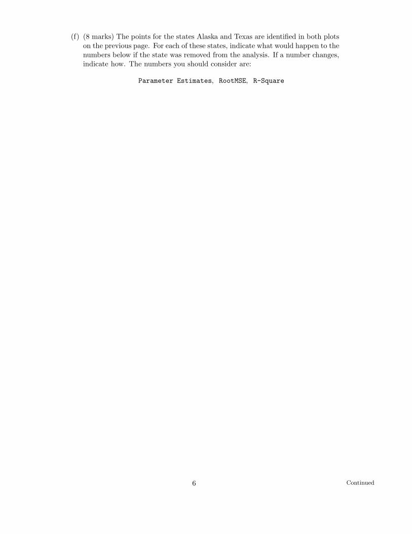
(f) (8 marks) The points for the states Alaska and Texas are identified in both plotson the previous page. For each of these states, indicate what would happen to thenumbers below if the state was removed from the analysis. If a number changes,indicate how. The numbers you should consider are:

Parameter Estimates, RootMSE, R-Square

6

Continued

2. For the mutiple linear regression model Y = Xβ + ε, the least squares estimates areb = (X′X)−1X′Y and the residuals are e = Y − Xb. Assume the Gauss-Markovconditions hold.

(a) (2 marks) Show that b is an unbiased estimator of β.

(b) (5 marks) Show Cov(b) = σ2(X′X)−1.

7

Continued

(c) (5 marks) Show e = (I−H)ε and Cov(e) = (I−H)σ2 where H = X(X′X)−1X′.

(d) (3 marks) Find Cov(Y) in terms of the matrix H, where Y = Xb.

8

Continued

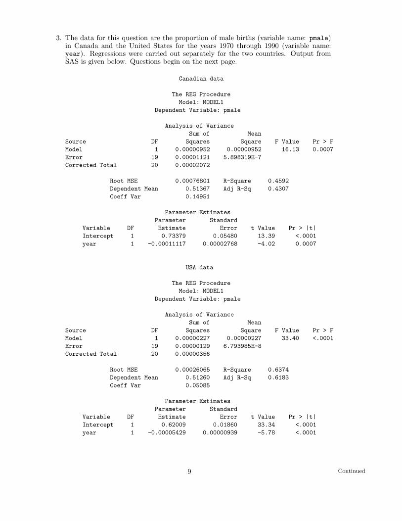
3. The data for this question are the proportion of male births (variable name: pmale)in Canada and the United States for the years 1970 through 1990 (variable name:year). Regressions were carried out separately for the two countries. Output fromSAS is given below. Questions begin on the next page.

Canadian data

The REG Procedure

Model: MODEL1

Dependent Variable: pmale


Sum of Mean


Model 1 0.00000952 0.00000952 16.13 0.0007

Error 19 0.00001121 5.898319E-7


Root MSE 0.00076801 R-Square 0.4592


Coeff Var 0.14951

Parameter Estimates

Parameter Standard


Intercept 1 0.73379 0.05480 13.39 <.0001

year 1 -0.00011117 0.00002768 -4.02 0.0007

USA data

The REG Procedure

Model: MODEL1

Dependent Variable: pmale


Sum of Mean


Model 1 0.00000227 0.00000227 33.40 <.0001

Error 19 0.00000129 6.793985E-8




Coeff Var 0.05085

Parameter Estimates

Parameter Standard


Intercept 1 0.62009 0.01860 33.34 <.0001

year 1 -0.00005429 0.00000939 -5.78 <.0001

9

Continued

(a) (4 marks) Are the proportions of male births on the decline in Canada and theU.S.? What can you conclude from these regressions to answer this question?

(b) (3 marks) Explain why the United States has the larger t statistic for the testof H0 : β1 = 0 even though its slope is closer to zero. Give both a statisticalexplanation and suggest a practical reason why this happened.

10

Continued

(c) (4 marks) Give an equation for a single linear model from whose fit both of theregression equations from the output above can be obtained. Be sure to defineall of your variables and explain how to test whether the change in the male birthrate differs between the two countries.

(d) (4 marks) On the next page there are residual plots for the regression of pmaleon year for Canada. What additional information about the data is provided bythese plots? How does this affect your answer to part (a) for Canada?

11

Continued12

Continued

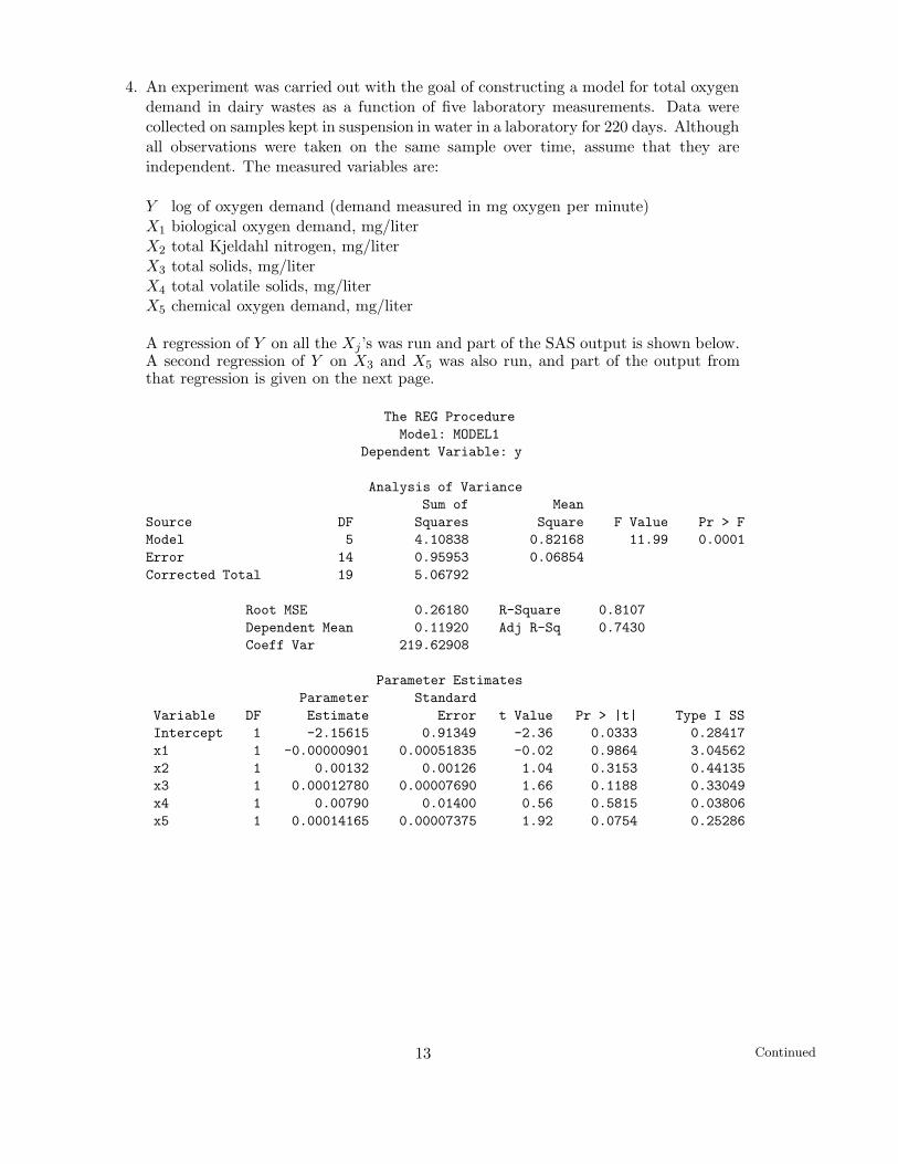
4. An experiment was carried out with the goal of constructing a model for total oxygendemand in dairy wastes as a function of five laboratory measurements. Data werecollected on samples kept in suspension in water in a laboratory for 220 days. Althoughall observations were taken on the same sample over time, assume that they areindependent. The measured variables are:

Y log of oxygen demand (demand measured in mg oxygen per minute)X1 biological oxygen demand, mg/literX2 total Kjeldahl nitrogen, mg/literX3 total solids, mg/literX4 total volatile solids, mg/literX5 chemical oxygen demand, mg/liter

A regression of Y on all the Xj’s was run and part of the SAS output is shown below.A second regression of Y on X3 and X5 was also run, and part of the output fromthat regression is given on the next page.

The REG Procedure

Model: MODEL1

Dependent Variable: y


Sum of Mean


Model 5 4.10838 0.82168 11.99 0.0001

Error 14 0.95953 0.06854




Coeff Var 219.62908

Parameter Estimates

Parameter Standard

Variable DF Estimate Error t Value Pr > |t| Type I SS

Intercept 1 -2.15615 0.91349 -2.36 0.0333 0.28417

x1 1 -0.00000901 0.00051835 -0.02 0.9864 3.04562

x2 1 0.00132 0.00126 1.04 0.3153 0.44135

x3 1 0.00012780 0.00007690 1.66 0.1188 0.33049

x4 1 0.00790 0.01400 0.56 0.5815 0.03806

x5 1 0.00014165 0.00007375 1.92 0.0754 0.25286

13

Continued

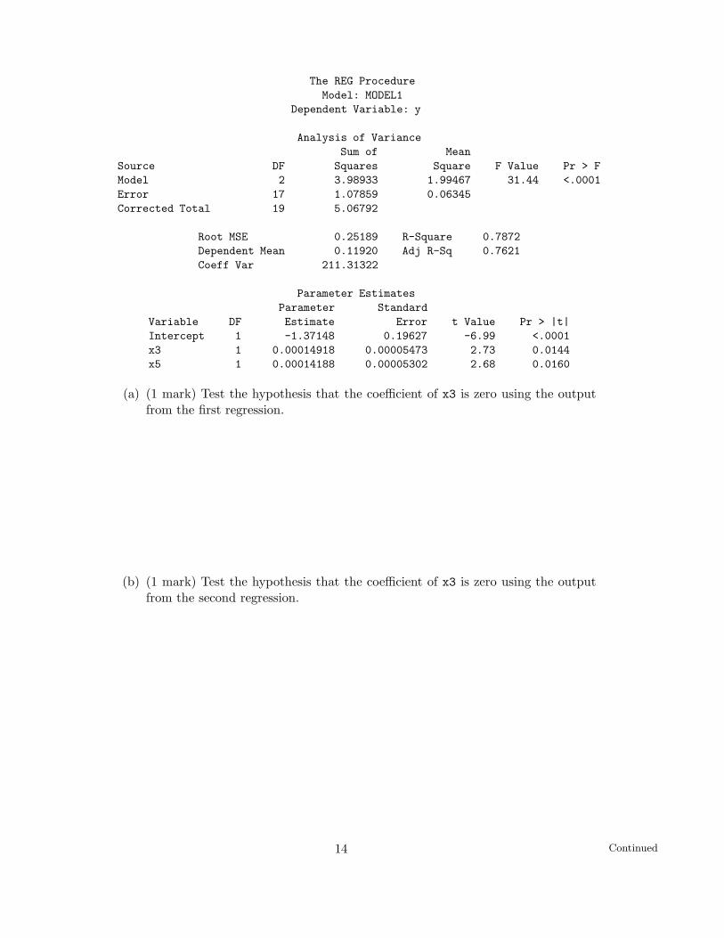
The REG Procedure

Model: MODEL1

Dependent Variable: y


Sum of Mean


Model 2 3.98933 1.99467 31.44 <.0001

Error 17 1.07859 0.06345




Coeff Var 211.31322

Parameter Estimates

Parameter Standard


Intercept 1 -1.37148 0.19627 -6.99 <.0001

x3 1 0.00014918 0.00005473 2.73 0.0144

x5 1 0.00014188 0.00005302 2.68 0.0160

(a) (1 mark) Test the hypothesis that the coefficient of x3 is zero using the outputfrom the first regression.

(b) (1 mark) Test the hypothesis that the coefficient of x3 is zero using the outputfrom the second regression.

14

Continued

(c) (2 marks) Explain why there is a difference in your answers to parts (a) and (b).

(d) (3 marks) State the null and alternative hypotheses for the Analysis of VarianceF test for the first regression. What conclusion do you draw from its p-value?(For the conclusion, do not say whether or not you reject the null hypothesis butrather say what the test tells you about the linear model.)

(e) (3 marks) Use the output from the first regression to test the joint hypothesisβ4 = 0, β5 = 0.

15

Continued

(f) (4 marks) Which model do you prefer? Justify your choice.

(g) (2 marks) What residual plots would you like to see to check whether it is rea-sonable to “treat the observations as independent”?

16

Continued

5. For each of the following questions, give brief answers (one or two sentences). Answerswithout explanation will not receive any marks.

(a) (2 marks) In a simple regression of weight on height for a sample of adult males,the estimated intercept is 5 kg. Interpret this value for someone who has nottaken any statistics courses.

(b) (2 marks) In simple linear regression, why can an R2 value close to 1 not be usedas evidence that the model is appropriate?

(c) (2 marks) Suppose that the variance of the estimated slope in the simple regres-sion of Y on X1 is 10. Suppose that X2 is added to the model, and that X2 isuncorrelated with X1. Will the variance of the coefficient of X1 still be 10?

17

(d) (2 marks) A regression analysis was carried out with response variable sales ofa product (Y ) and two predictor variables: the amount spent on print adver-tisements (X1) and the amount spent on television advertisements (X2) for theproduct. The fitted equation was Y = −2.35+2.36X1 +4.18X2 − .35X1X2. Thetest for whether the coefficient of the interaction term is zero had p-value lessthan 0.0001. Explain what this test means in practical terms for the companyexecutive who has never studied statistics.

(e) (2 marks) Explain why we might prefer to use adjusted R2 rather than R2 whencomparing two models.

18

Continued

6. (5 marks) A large real estate firm in Toronto has been keeping records on selling pricesfor single family dwellings. They have also recorded numerous other features of thehouses that sold, including square footage, number of rooms, property taxes, type ofheating, lot size, area of city, existence of finished basement, etc. An agent for thisfirm hopes to use these data to show that the rate of change in house prices over thepast seven years differs depending on area of the city. Describe how you would helpthe agent.

19

Continued20

Continued21

Total pages 22Total marks 90

Simple regression formulae

b1 =∑

(Xi−X)(Yi−Y )∑

(Xi−X)2b0 = Y − b1X

Var(b1) = σ2

∑

(Xi−X)2Var(b0) = σ2

(

1n

+ X2

∑

(Xi−X)2

)

Cov(b0, b1) = − σ2X∑

(Xi−X)2SSTO =

∑

(Yi − Y )2

SSE =∑

(Yi − Yi)2 SSR = b2

1

∑

(Xi −X)2 =∑

(Yi − Y )2

σ2{Y h} = Var(Y h) σ2{pred} = Var(Y h − Y h)

= σ2

(

1n

+ (Xh−X)2∑

(Xi−X)2

)

= σ2

(

1 + 1n

+ (Xh−X)2∑

(Xi−X)2

)

Xh ±tn−2,1−α/2

|b1|∗ appropriate s.e. Working-Hotelling coefficient:

(valid approximation if t2s2

b21

∑

(Xi−X)2is small) W =

√

2F2,n−2;1−α

Cov(X) = E[(X− EX)(X− EX)′] Cov(AX) = ACov(X)A′

= E(XX′) + (EX)(EX)′

b = (X′X)−1X′Y Cov(b) = σ2(X′X)−1

Y = Xb = HY e = Y − Y = (I−H)Y

H = X(X′X)−1X′ SSR = Y′(H− 1nJ)Y

SSE = Y′(I−H)Y SSTO = Y′(I− 1nJ)Y

R2adj = 1− (n− 1) MSE

SSTO

Cp =SSEp

MSEP− (n− 2p) PRESSp =

∑

(Yi − Yi(i)))2

22

faculty of arts and science sta 302 h1f / 1001 h1f

Documents