FACTORS INFLUENCING THE SUPPLY OF SUGAR: AN

ANALYSIS FOR KENYA 1970-2003

BY

FREDERICK K.^GITAIII

A RESEARCH PAPER SUBMITTED TO THE DEPARTMENT OF ECONOMICS,

UNIVERISTY OF NAIROBI IN PARTIAL FULFILMENT OF THE REQUIREMENT

FOR DEGREE IN MASTER OF ARTS IN ECONOMICS.

OCTOBER, 2004.

w .r - -ujessaj^

DECLARATION

This research paper is my original work and has not been presented for a degree

award in any other University

FREDERICK K. GITAHI...x5T.T^.:.............. ........ DatA qJ O J P ^ os

This paper has been submitted for examination with our approval as University

Supervisors.

MR. AWITI

n \

Dedication

Dedicated to my late parents Mr. Jacob Gitahi Kinini

And Mrs. Tabitha Nyathoko Gitahi.

in

AcknowledgementMy sincere thanks go to all people who contributed to the completion

o f this study. 1 am foremost grateful to my supervisors Mr. Awiti and

Dr Sule for their support, ideas and valuable feedback regarding the

materials in this research. They kindly advised and guided me up to

the completion of this research paper.

1 am also very grateful to all those institutions especially Kenya Sugar

Board and Meteorological Department that assisted in supplying the

necessary data for this study.

My sincere thanks also go to the M.A Economics students particularly

to Mr. Mike Ojuang’ and Mr. Joseph Tutoek for their academic

support.

I am also grateful to my family especially my wife Mrs. Miriam

Wanjiku Kariuki and my son Mr. Francis Gitahi Kariuki for their

material and moral support during my studies

I am especially very grateful to my brothers and sisters and in

particular Dr. Simon Ndung’u Gitahi and Dr. Clement Kanja Gitahi

for their moral, material and financial support during my schooling

To all those people and many others whom I could not mention by

name, my word is, I am grateful for assisting me in overcoming all

odds encountered in the cause of this study.

IV

List of Tables and Figures..............................................................Page1.1 World Sugar Production and Consumption (1964-1985)...................................................... 2

1.2 Annual Growth Rate of Real GDP................................................................................................ 4

1.3 Distribution of GDP by sector........................................................................................................4

14 Structural Adjustment Programme (SAPs) implementation process........................... 6

1.5 Area under Sugarcane by factory and Average Cane Yield....................................... II

1 6 Sugar Factories in Kenya: Rated Milling Capacity........................................................ 12

1.7 Sugar Supply and Demand in Kenya (1974-84), 1994-2003....................................................13

4.1 Summary Statistics......................................................................................................................... 37

4.2 Summary of Unit Root test............................................................................................................ 41

4.3 Regression Results.......................................................................................................................... 43

4.4 Short-run and Long-run Elasticities.............................................................................................. 47

APPENDIX...........................................................................................................................................54

1 Descriptive Statistics.......................................................................................................................54

2 Correlogram Test of Stationarity...................................................................................................55

3 Unit Root Results (ADF and PP test)............................................................................................ 58

4 Cointegration Analysis Results......................................................................................................60

6 Correlation Matrix........................................................................................................................... 60

5 Graph o f Residuals........................................................................................................................... 61

7 Regression Results (Long-run Equation)......................................................................................63

8 Regression results (Differenced Model)........................................................................................60

9 Regression Results Including Error Correction Model............................................................. 64

10 histogram for Residuals................................................................................................................ 65

11 Pairwise Granger Causality Test...................................................................................................66

12 Impulse Response Function (IRF)...............................................................................................67

v

List of AbbreviationsAFC Agricultural Finance Corporation

COMESA Common Market for Eastern and Southern Africa

CBS Central Bureau of Statistics

ESAF Enhanced Structural Adjustment Facility

ECM Error Correction Model

ICO International Sugar Organization

1CUMS A International Commission for Uniform Methods of Sugar Analysis

IRF Impulse Response Function

KBS Kenya Bureau of Standards

KSA Kenya Sugar Authority

KESREF Kenya Sugar Research Foundation

KMD Kenya Meteorological Department

SAPs Structural Adjustment Programme

VECM Vector Error Correction Model

vi

Abstract

Domestic demand for sugar in Kenya has continued to outstrip domestic production levels over

the last three decades Over the last ten years the country has registered an average annual deficit

in sugar production of one ninety thousand metric tones. This gap between domestic production

and domestic demand has to be met through importation.

The main objective of this study was to investigate the factors that influence supply of sugar in

Kenya with the aim of proposing policy measures to improve production.

The study found out that producer price, area under sugarcane and average annual rainfall and

structural policies implementation phase are significant factors influencing sugar production

The broad results indicate that improving producer price of sugarcane, acreage under sugarcane

and availability of water (e g through irrigation) would improve the quantity of sugarcane supplied

Results o f the study also indicate that implementation of structural adjustment policies adversely

affects sugarcane production.

Previous periods yields of sugarcane and the periods before introduction of SAI’s and SAPs

policy formulation stage were found not to influence sugarcane production. This may he attributed

to the fact that sugarcane is perishable industrial crop.

Policies recommended from the findings of the study include that producer prices be made more

favourable to sugarcane farmers, extensive methods of farming be enhanced and irrigation

methods be employed.

The short-run and long-run elasticities of output to various variables are equal implying that

policy impact on sugarcane production will persist into the future and have a permanent impact.

vn

Table of ContentsDeclaration................................................................................................................iiDedication.................................................................................................................iiiAcknowledgement.......................................................................................................ivList o f Tables and figures................................................................................. .......vList o f abbreviation......................................................................................................viabstract....................................................................................................................... vii

CHAPTER 1

1.0 Introduction......................................................................................... 1

1.1 Background to study....................................................................................... 1

1 2 Role of Agriculture in Economy..................................................................3

1.3 Kenya’s Economic Structure....................................................................... 3

1.2 Sugar Production in Kenya....................................................................................8

1.3 Organization of Kenya’s sugar Industry............................................................ 8

1.3.1 Performance of sugar Industry.................................................................... 10

1.3.2 Sugar cane production..................................................................................13

1.3.3 Sugar Milling Process..................................................................................14

1.3.4 Pricing and Distribution........................................................................................ .16

1.4 Statement of the Problem.................................................................................... 17

1.4.1 Objectives of Study.................................................................................... 18

1.4.2 Hypothesis.................................................................................................. 18

1.4.3 Significance of the Study..........................................................................19

CHAPTER 2

2.0 Literature Review................................................................................................21

2.1 Studies Outside Kenya........................................................................21

2.2 Studies in Kenya...................................................................................23

2.3 Overview of Literature.........................................................................26

CHAPTER 3

3.0 Methodology............................................................................................................28

3 1 Theoretical Framework............................................................................... 28

viii

3.1.1 The Model.................................................................................34

3.1.2 Estimation Technique..............................................................35

3.1.3 Data Types, Sources and Limitations................................... 35

CH A PTER 4

4.0 Final results.........................................................................................................36

4.1 Descriptive Analysis................................................................................36

4.1.1 Summary statistics of the variables........................................36

4.2 Stationarity Tests....................................................................................... 38

4.2.1 Graphical Approach................................................................38

4.2.2 Correlogram............................................................................. 39

4.2.3 Dickey-Fuller Unit root test...................................................40

4.3 Correlation Analysis...................................................................................40

4 4 Coitegration test......................................................................................... 41

4.4.1 Cointegration Result................................................................41

4.5 Empirical Results........................................................................................ 42

4.5.1 Final Estimation Results........................................................ 42

4.5.2 Interpretation........................................................................... 42

4.5.3 Error Correction Model.......................................................... 44

4.6 Structural Analysis..................................................................................... 44

4.6.1 Granger Causality Test........................................................... 45

4.6.2 Impulse Response Function....................................................45

4.7 Long-run and Short-run Elasticities........................................................ 45

CHAPTER 5

5.0 Conclusions And Recommendation.................................................................... 47

5.1 Policy Implication....................................................................................... 48

5.2 Suggestion for further research................................................................49

Bibliography................................................................................................................ 50

Appendix.........................................................................................................................54

ix

CHAPTER 1

1.0 INTRODUCTION

1.1. Background to Study

Sugarcane (Saccharum Officinarum) grows in the equatorial region and the tropics and warm

temperate zones between 35° North and 35° South. On average sugarcane requires a minimum

rainfall o f 1000 mm well distributed throughout the year, but optimum rainfall requirement is

1500 mm if satisfactory growth and yield are to be realized. Altitude with its moderating effect

on temperature has a significant impact upon duration of sugarcane maturity and subsequent

length o f the crop cycle (Odada & Awiti, et al 1986). Sugarcane is only but one source of sugar

consumed in the world, beet, produced in the temperate zones, has been for a long time a

significant source of sugar. There has also been a significant move in the production of sugar

from corn

The sugarcane industry is one o f the oldest food processing industries in the world Writers on

ancient civilizations in Egypt and India reckon that sugar extraction from sugarcane was part and

parcel o f these civilizations. As civilization spread to Western Europe, sugar extraction from

sugarcane became a significant process of the transfer of technology in those medieval days.

The Industrial Revolution in the 17th century in Europe gave the industry a big boost to the extent

that sugar became “white gold” because of its profitability. The sugar industry was the

cornerstone of the “triangular trade” which began with tradables from Europe being taken to

Africa to be bartered for slaves. The slaves were exchanged in the West Indies for sugar which

was then shipped to Europe

In 1964, contributions of developed and developing countries to world supply of sugar were

more or less equal By 1982, the developing countries share in total world sugar production had

increased to 60%. The rate o f increase in sugar production has been higher in developing

countries.

1

The following table shows world sugar production and consumption for the period 1964 to 1985

Table 1,1 World Sugar Production and Consumption (1964-1985) (million ionnesj

1964-1966 1968-1971 1974-1976 1979-1981 1982 1985

Production

Developed

Countries 31.7 32.7 33.6 37.1 38 6 39 7

Developing

Countries • 31.5 38.0 35.9 51.3 62 8 60 2

Total 63.2 70.7 69.5 88.4 101.4 99.9

ConsuniDtion

Developed

Countries

39.6 42.0 44.3 44.0 44.0 45.0

Developing

Countries

23.6 28.6 34.9 44.0 48.0 53.2

Total 63.2 70.6 79.2 88.0 92.0 98.2

Source: World Food Prospectus, various

The highest level of world sugar production was attained in 1982 when production reached on all

time pick o f 101.4 million tonnes By 1964, developed countries had a higher rate of sugar

consumption than developing countries.

The major world producers o f sugar are: India, Brazil and Cuba while in Africa, the leading

sugar producing countries are South Africa, Egypt, Mauritius, Swaziland and Zimbabwe in that

2

order (International Sugar Organization, 2002). By international standards. Kenya is considered

a marginal producer of sugar.

1.2 Role of Agriculture in the Economy

Agriculture accounts for almost 25% of GDP (Statistical Abstract - 2003).

Sessional Paper No. 1 of 1986 spelt out the goals of the agricultural sector to the year 2000 Self-

sufficiency in foodstuffs and food security is stressed as the long-run goal In the shoit-mn.

appropriate policies need to be formulated to revitalize the sugar sub-sector and enable it attain

long-run goals. Contrary to these intended goals as spelt out in Sessional Paper no. 1 of I'>86, the

trend depicted by the table 1.5 shows that demand continues to outstrip domestic supply and that

the shortfall is expanding. This means that both short-run and long-run sugar policies need to be

amended to reverse the trend.

1.3 Kenya’s Economic Structure

The macro-economic performance of the Kenyan economy since independence can be assessed

in the context of external shocks and internal challenges that the economy has had to adjust to.

Four phases are identifiable a rapid economic growth phase over the period 1964-73, an era of

external shdeks over 1974-79 dominated by oil shocks and coffee boom, a period of stabilization

and structural adjustment in the 1980s and an era o f liberalization and declining donor inflows

from 1990s to date The overall effects of changing circumstances have been a declining trend as

shown in table 1.2.

Kenya’s Economic structure comprises of monetary and non-monetary sectors. In the monetary

sector, agriculture continues to be the dominant sector followed by government services and then

manufacturing.

Kuznets (1966) postulated that for a country to industrialize, the contribution of agricultural

sector to GDP tend decline and contribution of industrial sector (manufacturing) tend increase

From the table 1.2 it is clear that growth rates of GDP in both agriculture and manufacturing

have been declining over time. This means that the decline in the agriculture is not being

compensated by growth in the industrial sector. There is no evidence o f structural shift from

agriculture to industrial sector. Therefore the decline in growth in the agricultural sector is not

due to the process of industrialization. Manufacturing registered a marginal growth in

contribution to GDP from 10.6 % in the period 1964-73 to 13.3 % for the period 1996-2000

3

GDP growth rate is projected to improve to 4 per cent in the period 2001-2008(Development

Plan, 2002).

Table 1.2 Annual Growth Rate of Real GDP (%)

Sector 1964-73 1974-79 1980-89 1990-95 1996-2000 2001-

08*

Agriculture 4.6 3.9 3.3 0.4 1.1 3.3

Manufacturing 9.1 10.0 4.8 3.0 1.3 3.3

GDP 6.6 5.2 4.1 2.5 2.0 4.0

Source National Development Plan, Statistical Abstract, various

Table 1 3 Distribution of GDP bv sector (%)

Sector 1964-73 1974-79 1980-89 1990-95 1996- 2001-

2000 2008*

Agriculture 36.6 33.2 29.8 26.2 24.5 22.4

Manufacturing 10.6 11.8 12.8 13.6 13 3 12.2

Source National Development Plan, Statistical Abstract, various

* projected

In 2002-2008 National Development Plan, the government re-asserted its aim of revitalizing the

sugar industry to ensure adequate supplies for local consumption.

In the decade 1963-73, Kenya’s economy grew at high rates, with GDP expanding by 6 6 per

cent per annum This was due to increased agricultural output; expansion of manufacturing

sector supported by adoption of import substitution strategies; rising domestic demand,

expansion of the regional markets and substantial inflows of foreign aid Fluctuating world prices

of agricultural products and the oil crisis reversed the impressive economic performance

experienced in the first decade. The first oil crisis of 1973 brought an abrupt decline in economic

growth rate. The growth rate declined to below 4 per cent except for 1976/77 when the

unexpected coffee boom saw the GDP grow at 8.2 in 1977. The collapse of the East African

Community (EAC) in 1977 and the second oil crisis o f 1979 contributed to further deceleration

in economic performance.

4

Unfavourable weather conditions experienced in the early 1980s, world recession and the

international debt crisis worsened the domestic economic situation The 1980s was also

characterized with misaligned real exchange rates, fixed exchange rate regime as well as pool

commodity pricing which all acted to undermine macroeconomic stability. To address the

macroeconomic instability the government introduced liberalization and deregulation of trade

and exchange rate regimes, public and financial sector reforms through tire SAI’s

programme.Table 1.4 summarizes the SAPs programme process as implemented in the

agricultural sector

In 1980 Kenya formally adopted the Structural Adjustment Programme (SAPs) which was being

advocated by World Bank and IMF and was aimed at achieving structural changes and attain

high levels of economic development. Between 1980 and 1985 the reform was mainly in policy

matters.

In the second half o f 1980s, there was gradual actual implementation of policies The

programme was characterized with liberalization of trade and prices including agricultural prices

and foreign exchange decontrols. The SAPS meant that from mid 1980s, Kenya experienced

changes affecting all the sectors o f the economy. The sugar cane industry was liberalized in that

period and there was free trade in sugar.

Before mid 1980s, the government controlled the sugar industry. The government was

controlling the supply o f sugar, pricing and marketing as well industry’s processing.

5

Table 1.4 SAPS implementation process

TYPE OF POLICY

INTRUMENTS

MACROECONOMIC

INTRUMENTS

AGRICULTURAL SECTOR

INTRUMENTS

Pricing policy

Exchange rate

Wage rate

Interest rates

Output prices (Administered),

Wage rate

Irrigation charges

Agricultural interest rates

Fiscal policy

Subsidies, Tax rates, Public

investment

Subsidies, Tax rates

Public investment•

Monetary policy

Money supply, target

interest rate, Credit

allocation

Agricultural credit targets

Agricultural interest rate

Trade policy

Tariffs and quotas

Export subsidies

Tariffs and quotas

Export subsidies

Institutional reforms

Monetary management

rules, Management o f

parastatals, Divestiture in

public enterprises

Marketing Boards reforms,

Reduction of intermediation

costs in agricultural banks.

Improved agricultural research

Land policy

Cadastral survey plans

Land taxes/levies

Zoning

Land taxes/levies, Land Titling,

Sale Policy o f Public land

Consolidation o f scattered

parcels

Source: Food Security, Food aid and Structural Adjustment in Agriculture, pg 9

In introducing the SAPs programme, the expectation was that agricultural sector would respond

to SAPs policy changes through increased agricultural supply of exports, help restore balance of

6

trade and assist in moderating domestic inflation and contribute to the process of internal

adjustment through increased food production.

The SAPs reform programme has been criticized on the grounds that a market-based approach is

inappropriate due to market imperfections in many sub-Saharan African countries (Obidegwu,

1990).

In Kenya, a study by Mwega (1995) concluded that trade liberalization, including the agricultural

sector, arising from SAPs does not seem to be positively correlated with productivity growth but

is positively correlated with output and employment growth in the manufacturing sector

In the 1990s and early 2000s, poor economic performance can be attributed to declining donor

funds, poor weather and infrastructure; insecurity; declining tourism activities and poor

performance of the manufacturing sector. Overall GDP growth declined further to 2.5 per cent

between 1990 and 1995 to 2 per cent between 19996 and 2000. The decline in economic

performance was apparent in all the sectors of the economy.

Liberalization of the economy introduced major changes in marketing and pricing of sugar

Before introduction of SAPs, importation of sugar was controlled by the government by

licensing particular importers/ agents and allocating import quotas through Kenya Sugar

Authority. Uncontrolled imports of white sugar which is more refined than locally produced

sugar found its way to the domestic market. Its importation is done by private firms and

individuals. The SAPs programme therefore introduced competition between local sugar firms

and sugar importers. Tariff on sugar imports is aimed at bringing prices for imported sugar to a

level which represent reasonable remuneration for the efficient producer at an acceptable level of

risk This is because the price at which sugar can be imported from the world market at any one

time bears little or no relation to the cost of producing that sugar. A possible reason of low prices

of imported sugar is application of agricultural subsidy policies in source countries and more

efficient production methods. A sugar importing country that fully exposes its domestic industry

to world prices faces negative impacts to development of sugar-based industries

7

1.2 Sugar Production in Kenya

Sugarcane production in Kenya on a commercial basis was started in 1922 when the Miwatii

Sugar Mills Limited established a medium-scale sugar mill at Miwani in Kisumu District of

Nyanza Province. A second sugar company was established in 1927 by Associated Sugar

Company at Ramisi in Kwale District of Coast Province. These sugar mills were owned by and

managed almost exclusively by Asians. African farmers started playing a major role in the

production of sugarcane when two additional sugar mills were established by Kenyan

Government in Kisumu District. These were the African Sugar Company Limited at Muhoroni

(1966) and Chemilil Sugar Company Limited (1967). Establishment of the two sugar schemes

saw the beginning of direct participation of the Kenya Government in the sugar industry’ in the

form of ownership

A fifth sugar mill was established by the Kenya Government at Mumias in Kakamega District of

Western Province in 1973. This was followed by a sixth sugar mill at Nzoia in Bungoma district

o f Western Province. A seventh sugar (Sony) mill was established in 1979 at Awendo in South

Nyanza Province. The establishment of these large-scale sugar schemes led to a significant

increase in domestic supply o f sugar in Kenya since the mid 1960s, and led the country to self

sufficiency in sugar in 1979 (see table 1.7) below. In 1994, West Kenya Sugar Company was

established in Western Province. Miwani Sugar Mill was closed down indefinitely in February

2002 while Ramisi was closed down in 1988.

1.3 ORGANISATION STRUCTURE OF KENYA’S SUGAR INDUSTRY

In Kenya cane is grown either in the nucleus estates, by outgrowers or contracted farmers The

nucleus estates (Plantations) are large parcels of land owned by the factory establishment. The

nucleus estates are established to provide buffer against risk of inadequate cane supplies from out

growers, provide sugar companies with a base for scientific research and cane husbandly and

provide land facilities for the introduction of new sugar cane varieties

The out growers can be divided into four district categories: large scale farms, small-scale farms,

cooperatives and settlement schemes. The large-scale farmers are concentrated in the Nyanza

Sugar Belt where they deliver cane to Chemilil, Muhoroni and Miwani Sugar factories.

Cooperative sugarcane farming is least developed and is found in Nyanza Sugar Belt (mainly

8

Chemilil and Miwani Sugar Schemes). Settlement Schemes Sugarcane farmers deliver cane to

Muhoroni and Chemilil Sugar factories Area under cane for outgrowers, nucleus estates and

contract farmers and the average cane yield for the various factories for 2003 is shown table 1.5.

Table 1.5 Area Under Sugarcane By Factory And Average Cane Yield-2003

Factory

Area Under Cane (hectares)

Average Cane Yield

(Tonnes/ha)

Outgrowers Nucleus Contract

Farmers

Chemilil 9256 2017 - 63 38

Muhoroni 8305 1345 - 57.10

Mumias 45031 3432 - 75 93

Nzoia 13160 3333 - 74.75

Sony 10807 2270 - 77.66

West Kenya 6240 1850 - 69.25

Miwani* ** 6300— — -

Ramisi"— — — —

Source Kenya Sugar ioard, 2004

* closed down at beginning of 2002

** closed down in 1988

Mumias Sugar factory has the greatest area under cane for both the outgrowers and nucleus

estate while Miwani had the smallest. Average cane yield ( i.e. no of tonnes of processed sugar

per hectare) is highest in Sony Sugar mill and smallest in Mumias sugar mill. The average cane

yield may be affected by cane variety and relative efficiency of factories in sugar processing

Table 1.6 Summaries information on the six major sugar factories which are operational

9

Table 1.6 Sugar Factories In Kenya- Annual Rated Milling Capacity (At Inception)

Factory Year o f Establishment Rated milling capacity of

sugar(1000’Metric tonnes)

Muhoroni 1966 60,000

Chemelil 1967 55,000

Mumias 1973 180,000

Nzoia 1978 60,000

Sony 1979 60,000

West Kenya 1994 50,000

Source. Kenya Sugar Board, 2004

The rated milling capacity is number of tonnes of sugar the factory is capable of processing per

year, assuming adequate cane supply and allowance for servicing of machines The figures

reflected above show the rated capacity of the factories at the time of inception and are expected

to decrease over time due to depreciation or some machines being rendered obsolete due to

changes in technology. The factories operate with excess capacity due to inadequate supply of

cane Seasonal fluctuations of cane supply may also force the factories to operate at sub-optimal

capacity. Mumias factory has the highest milling capacity while West Kenya which was

established in 1994 had the lowest.

1.3.1 Performance of the sugar industry

The performance of the agricultural sector in general in the decade 1964- i >74 was impressive

It’s contribution to GDP in that period was 36.6 per cent but declined to 26.2 per cent in 1990-

1995 and 24.5 percent in the period 1996-2000 and is projected to contribute to GDP at an

average share of 22 4 per cent over the period 2001-2008(see table 1.3).

The performance of the sugar sub-sector shows that demand continues to outstrip supply

(production) which means that the deficit must be met through sugar importation

The following table depicts sugar production and consumption Kenya for the periods 1974-1984

and 1994-2003.

10

The table shows there was declining deficit in the period 1974-1978 and a movement towards

self- sufficiency reflected by the surplus between 1979-1982. The trend was reversed in 1983

and from 1994 there was a large deficit in sugar supply.

Consumption in general depicts an increasing trend while production depicts a

mixed trend and increased between 1994 and 1999, then registered huge decline in

2000-2001 with improvements in production in 2002-2003. Despite mixed

performance in the production, domestic production was less than domestic

demand in the entire period 1994-2003.

11

Table 1.7 Sugar Supply And Demand In Kenya: (000’ Metric Tones) 1974-84; 1994-2003

Year Production Consumption Deficit/Surplus

1974 163 224 -61

1975 180 203 -23

1976 170 195 -25

1977 185 200 -15

1978 238 260 -22

1979 296 253 43

1980 383 296 87

1981 368 367 1

1982 353 348 5

1983 325 333 -8

1984 371 380 -9

1994 387.5 566.2 -178.7

1995 388.6 563.5 -174.9

1996 389.0 570.0 -181.0

1997 401.6 580.6 -179.0

1998 449.1 587.2 -138 1

1999 470.7 6094 -138.7

2000 401.9 631.2 -229.3

2001 377.4 644 5 -267.1

2002 494.2 680.5 -186.3

2003 448.5 691.6 -243.1

Source: Kenya Sugar Board, 2004

To fill the gap between domestic production and consumption, the country is forced to import

sugar To reduce importation, the country has to increase domestically produced sugar to the

level of consumption. The industry, however, is faced with a number of constraints and

12

challenges that may hinder realization of full potential. Decline in sugar production may be due

to failure by the farmers to supply cane to factories because of reduced cane producer prices,

unfavourable weather conditions, and increased imports (Economic Survey 2004). I lowever only

a comprehensive empirical study can investigate the underlying factors that have resulted in

underproduction o f sugarcane which has been unable to meet domestic demand over the years

1.3.2 Sugar Cane Production

Production o f sugarcane involves a number of mechanical operations right from the beginning

until the crop is established, mature and harvested In the initial stage, mechanical operations

aimed at preparing suitable seed bed for cane planting are carried out Where land is virgin,

capital investment in bush clearing, de-stumping and land formation (leveling and grading)

needs to be undertaken

The soil is opened up by one round of deep ploughing and two rounds of light ploughing

Harrowing is then done to ensure a suitable soil tilth After harrowing, sugarcane field is

furrowed to make appropriate beds for seed cane. Sugarcane is a semi-permanent crop which is

normally harvested at least three times before uprooting to plant a new sugarcane crop I he first

sugarcane crop is known as “plant crop”. The subsequent crops, before uprooting are known

respectively as the “first ratoon” and “second ratoon” crops. While the plant crop normally

matures in 22-24 months, the ratoon crops mature in 18-24 months. A complete sugarcane crop

cycle thus takes about five years from the establishment o f a plant crop to the harvest of a second

ratoon crop.

Apart from geo-physical and climatic factors, sugarcane yields depend upon the qualities ot

initial land preparation, the seed cane and crop maintenance after establishment Various

varieties of sugarcane have different yields. However data on the various yields is not obtainable

from factories as they pay a uniform price for cane delivered, irrespective o f cane variety

Because sugarcane is a semi-permanent crop it is important to plant appropriate seed cane

varieties which should come from nurseries which had been established from heat-treated

sugarcane as a control measure against ratoon stunting disease. However, a number ol sugar

13

companies supply their outgrowers with ordinary cane for planting due to scarcities of such

nurseries.

Sugar cane requires nitrogenous, potassium or phosphate fertilizers and lime. For the small-scale

farmer, the main agents who distribute these inputs are the sugar companies

The common practice is to cut seed cane into three-node pieces known as “setts” . These are then

planted end to end in the furrow-beds and buried with soil. The most suitable time for planting is

during rainy season from March to May and from September to November.

For good yields, sugarcane should be kept weed-free throughout its complete cycle. Hand

weeding is widely adopted in all the sugar schemes except in Chemelil and Muhoroni where

combination o f hand weeding and chemical weed control are used.

Cane is harvested when it is considered mature and millable. In all the sugar schemes in Kenya,

cane is cut by hand labour. In some schemes, mainly in Nyanza Sugar Belt, cane is burnt before

harvesting to make the operation less cumbersome in both nucleus estates and out growers

schemes.

The harvested cane is then loaded onto tractors or lorries and delivered to sugar companies.

Although the sugar companies own most of transport facilities, a large number ol private

contractors and individuals have been attracted to this lucrative business. Cane arrives at the

factory gates where the carriers are weighed together with the cane on arrival and re-wciglied

after they have been unloaded to determine quantity of cane delivered. At this stage the cane

begins the manufacturing process which is described below.

1.3.3 Sugar Milling Process

Sugar cane processing to produce refined sugar is a capital-intensive process Alternative use of

sugar cane (e g in the brewing o f local liquors) is prohibited by law, and therefore household

consumption is negligible. In this respect sugar cane farming differs with other food crops

14

where peasant families consume substantial proportion of their food production. Therefore the

total production by farmers is also the total marketed production. In case of sugar cane industry,

production per given period can be regarded as supply per the same period as sugar cane cannot

be stored for future marketing as it is a highly perishable good, even if farmers expect higher

prices in the future.

There are a number o f stages in the processing of sugar. After off-loading, it is conveyed to

cutting stage for milling. At the milling stage, the mass passed on, crushed and squeezed to

extract juice from cane. The juice is then separated from waste material - (bagasse). Bagasse

which is the fibrous stem after extraction of juice is used as fuel for the boilers. This use of waste

material as an input in the production process substantially reduce production costs

The juice is then strained through screens and heated, limed and phosphated to prevent

conversion of sucrose into simple sugars. This process known as “clarification of the juice”

results in precipitation and separation of suspended matter and soluble non-sugars in the juice

The juice is then led to evaporators where further boiling takes place in low pressure to remove

impurities while darkening or browning due to burning is avoided.

The next process is crystallization where the thick syrup obtained from evaporators is fed to

vacuum pans where the sugar saturated mixture of molasses and sucrose forms the massecuite.

The massecuite is then purged into automatic centrifugal with a modicum of washing which

separates the sugar crystals from molasses. The sugar crystals are then dried and bagged in 100

kg bags ready for distribution.

The bulk o f the sugar produced in Kenya is known as mill-white sugar. It has a brownish

colour due to incomplete removal o f molasses coating. The extent of brownness varies with

factory to factory, depending on the extent of processing method and the weather conditions

prevailing at the time cane is harvested.

The Kenya government has put a minimum quality standards as regards colour and content o f

impurities in sugar in line with requirements o f International Sugar Organization (ISO). This

15

standard is based on International Commission for Uniform Methods o f Sugar Analysis

(ICUMSA) unit. The Kenya Bureau o f Standards regulates the quality of domestic sugar

1.3.4 Pricing and Distribution

Sugar factories usually do delivery o f sugar cane from the farms to sugar factories. I he prices

that are charged for farm level mechanical services are set out by Kenya Sugar Board in terms o f

amount per hectare or per hour specified capacities of the equipment used

As with many agricultural crops, the short-run supply of sugar cane is fixed as farmers will not

be able to respond immediately to changes in producer prices As with other agricultural

commodities, there is a time lag between which supply can respond to changes in various

explanatory variables The adjustment process between production and various factors depend

on technology being employed by the farmcrs(Odada, 1986)

Sugar cane farmers sell their produce to particular factories as they are controlled bv the zoning

system Because o f the single buyer in a particular region, the sugar factory is faced with an

upward-sloping supply curve, which shows the quantity of sugar cane supplied to it bv the

farmers at different producer prices it pays to the farmers, subject to a reserve price that is

expected to meet the production costs of a unit of sugar cane delivered to it by the farmer I he

supply of sugar cane that farmers can supply to sugar industries is constrained by other factors

apart from producer prices like cane variety, soil type, farming methods, weather, land and input

prices. Reserve price is usually recommended price by farmers associations but sugar firms may

choose not to go by it The price paid to the farmer for his sugar cane is therefore not determined

by the competitive markets. The sugar firms buy all the sugar cane delivered by farmers from a

particular zone

The price to farmers is determined by sugar factories that buy the sugar cane, add value by

processing and then sell the finished product (refined sugar) to specified distributors to supply to

16

retailers. However, because sugarcane is a perennial crop, substitutability with other food crops

with shorter gestation period is difficult.

Sugarcane-processing industries, like other multinationals, are profit maximizing but are

restrained by the fact that they buy sugar cane at a price that is equal or greater than the

production cost o f sugar cane to the farmer, otherwise the farmer would substitute sugar cane

with other crops (e g. maize, sorghum and millet) that grow in the same ecological zone as sugar

cane and are apparent substitutes. However in the short-run, prices of these crops are unlikely to

affect sugar supply as cane due to its semi-permanent nature.

No special financing of farmers is made by the sugar factories and the form of credit is offered is

in seeds and transport. The factories then recover these costs from the proceeds of the farmers

Sugar cane market can therefore be regarded as a case of monopsonistic buyer (sugar-cane

processing industries) operating under a restricted market due to zoning system, and the factories

then market the refined sugar oligopolistically through appointed agents (distributors) The

monopsonistic nature of sugar industries may result in consumer surplus in favour of sugar

industries.

1.4 STATEMENT OF THE PROBLEM

Over the last two decades consumption of sugar in Kenya has continued to outstrip supply and

therefore necessitating importation to fill the gap.

Sugar imports drain the country’s foreign exchange as resources meant for investment in other

sectors of the economy, including agricultural sector, are depleted

When a country relies on food imports, it creates a balance of payment crisis Due to lack of

foreign exchange, the country borrows both internally and externally to finance food imports,

and this leaves little for investment by the government in the social services as a large proportion

of revenue due to government is used in debt servicing. In developing countries, this may lead to

debt crisis. Borrowing by government also crowds out private investment through high interest

rates which increase cost of credit. The National Development Plan 2002-2008 spells out the

17

government commitment in achieving self-sufficiency in basic foodstuffs in order to allow the

nation to be fed without using scarce foreign exchange.

Given this gap between domestically supplied and consumed sugar and the possibility of BOP

deficits and debt crisis, there is need to intensify domestic sugar supply to enable the country to

be self reliant. The problem is on the supply side, which has to be raised to the level of domestic

demand.

Sugar is a commodity that does not have close substitutes and demand for sugar is likely to

increase with increase in population, as there is no likelihood of a decrease in consumption

More emphasis is therefore put on the supply side in order to save foreign exchange and the

sugar cane farmer. The level of importation, given the decrease or marginal increases in

domestic production, is likely to increase with increase in domestic demand arising from increase

in population.

The study will try to identify the factors that influence supply o f sugar and their relative

importance.

1.5 Objective of Study

The objectives o f the study are as follows:

(i) To identify the factors that influence sugar supply in Kenya.

(ii) To estimate the impact of these factors on sugar supply including the role of

SAPs.

(iii) Estimate the short-run and long-run elasticities of supply of sugar

(IV) To draw short-run and long-run policy recommendation from (i) and (ii)

above

The production of sugar cane is likely to be affected by many factors such as producer price,

hectarage under cultivation, SAPs, rainfall, marketing, sugar imports seed variety, soil type and

other unpredictable factors.

18

1.6 Hypothesis

This study will attempt to test the following hypothesis. For each variable, the null hypothesis I In

will be tested against the alternative hypothesis Hi.

1. H0 : A positive relationship exists between supply of sugarcane and

producer price to sugarcane farmers

Hi: No relationship exists between the two.

2. H0 : A positive relationship exists between supply o f sugarcane and

hectarage of sugarcane planted by farmers.

Hi: No relationship exists between the two.

3. Ho: A positive relationship exists between supply of sugarcane and

Mean annual rainfall in sugar growing zone

Hi: No relationship exists between the two.

4. Ho: The phases of SAPs program are significantly different from no SAPs

Hi: No significant differences exist.

5. H0 : A positive relationship exists between supply of sugarcane in current

period (t) and period (t-2).

Hi: No relationship exists between the two.

Data on the appropriate variables to estimate regression coefficients will be collected, diagnostic

tests conducted and the data analyzed The effects of the qualitative variable (SAPs) will be

captured through SAPs dummies. T-test will be carried out to assess the significance of

coefficients and appropriate inferences made Both short- and long-run elasticities will be

derived from regression coefficients

17 Significance of the Study

Sugar cane is an industrial crop that generate income to farmers and provide raw material to the

sugar-based industries which are capable of providing gainful employment to a large proportion

of Kenya’s total agricultural labour force. The sugar cane crop enterprise will be able to fulfill

these functions through multiplier effects only when sufficient incomes accrue to sugar cane

farmers to enable then expand sugar cane production and leave them with subsistence for their

19

immediate needs. There is therefore need to investigate the various factors that influence sugar

supply in Kenya.

The study attempts to give policy guidelines that may be used by the authorities to increase

domestic sugar production. The study will also provide useful guideline information to sugar

management bodies on how the liberalization o f the agricultural sector has affected the sugar

industry in Kenya. Besides, it is hoped that this study will serve as a starting point to people

wishing to pursue further studies in the sugar industry. It will also add value to the existing body

of knowledge on the Kenyan sugar sector. Finally, the study will be of great importance to the

sugar industry and policy makers.

In the last half o f 1980s and early 1990s, Kenya experienced a lot of changes affecting all sectors

of the economy. The sugar sector was liberalized in that period and there was free trade in sugar.

Previous studies did not investigate the effects o f SAPs policies on sugar sector, since all the

industry’s processes were being controlled by the government, from marketing of sugar cane,

processing, pricing to distribution. According to COMESA Act of 2002, Kenya’s quota of

importation of sugar is 89,000 tonnes o f common sugar and 111,000 tonnes o f industrial sugar.

Despite COMESA regulation imported sugar still finds its way into the country through the black

market.

This study will add value to previous studies as it evaluates the temporal effects of SAPs

policies.

This study is different from previous studies in that it will estimate the short-run and long run

elasticities of supply of sugar and aims at evaluating the supply of sugar in a liberalized

economy. The study is also essentially differs from other studies in that it aims at carrying out

structural analysis o f the sugar supply in the study period.

20

CHAPTER 2

2.0 LITERATURE REVIEW

2.1 Studies outside Kenya

Many previous studies of supply o f agricultural commodities and covering a wide range of

agricultural crops have been conducted in Kenya and other developing countries.

Krishna (1963) estimated supply elasticities for sugarcane, cotton, rice, millet, wheat and bailey

in the Punjab region and obtained short-run supply elasticities ranging from 0.08 for wheat to

0 72 for cotton and long-run elasticities ranging from 0.14 for wheat to 1 62 for cotton The study

used Nerlovian Partial Adjustment Model.

Bond (1983) conducted a study to estimate aggregate agricultural response to real producer

prices in sub-Saharan African countries, namely Ghana, Cote D’ivore, Kenya, Liberia,

Madagascar, Senegal, Tanzania, Uganda and Burkina Faso He developed his estimation

equation by assuming that the actual changes in output (Qt) in relation to previous existing level

( 0 t-i) is only some fraction of the change required to achieve equilibrium level (Q t)

Ln Q, - Ln Q,_i =P(Ln (2, - Ln Q,.()........................................................................................... (i)

He further postulated that equilibrium output (Qt ) depend on the aggregate real producer price

(P(), a time trend (t) to take into account the effects of long-run equilibrium output, and a dummy

variable (Z,) to capture the influences o f usual weather pattern

The estimating equation was

Ln Qi = p0+ Pi LnPt +P2LnQ,.i + P3t + P4Z, .................................................................. (ii)

The regression analysis showed that the relative price coefficient were positive in all countries

studied and that long-run price elasticity was greater than short-run elasticities in Ghana, Kenya,

21

Liberia, Madagascar, Uganda and Burkina Faso. The study can be criticized on the ground that

aggregate function for each country is obtained by adding across supply functions of individual

crops, therefore it ignores the fact that individual crops react quite differently to changes in price.

Ramesh et al (1988) using time series data for the period 1960/61 to 1984/85 carried out a supply

study aimed at examining the supply responsiveness of rice in India. His investigation reveals

that there is a positive supply response to price incentive in developing countries I lovvever, the

magnitude varies according to nature o f crop and between regions He also separated area and

yield responses models using Nerlovian lagged adjusted model. Yield was found to be

responsive to prices, but area less so as cropping patterns tended to be more or less established.

He concluded that the scope for increasing area under rice is limited unless a major irrigation is

undertaken.

Binswanger, et al (1987) used a sample of 58 countries for the period 1969-1978 to analyze and

determine the role of price and non-price factors on agricultural supply. The cross-country

analysis, according to this study, is useful in understanding the implications of choice of

technology on supply responses.

An interesting aspect of the study is the way variables are represented in the model, for instance,

extension services are measured by the number of extension agent per capita o f farm production,

irrigation as a percent of agricultural land irrigated at least once during the year, research by

number of years of training taken to convert workers into stock of scientists, the human capital

by adult literacy and life expectancy.

The model was estimated by single equation technique but the large number o f variables created

the problem of multicollinearity. The results indicated that the variables as a group account for

most variation in supply both within- country and between-country analysis. The results also

show that the within country (time series) elasticity with respect to non-price is small around 0.1 -

0 2 (short-run elasticity) and that the cross-country elasticity is negative.

22

Ssmogerere (1990) investigated the effects of SAP policies on the supply condition of coffee in

Uganda The study used qualitative data due to lack o f quantitative data She used a supply

model which assumed that acreage under coffee-yielding is fixed in the short-run, and might

remain fixed even in the long-run if coffee is grown in densely populated areas where land is

scarce. The study concentrated on the determinants o f changes of output per acre on land

productivity, to which variation of labour can be used in the short-run, and technological

improvement, purchase input and tree planting can be applied in the long-run The standard

equation of the model is

Log(Q/H) =a0 + ailog P, - a2 log Pt* - a3 log Z, + &jlog (1/r)

The study postulates that output per hectare (Q/H) is affected by the own producer price

elasticity of supply, the price elasticity of substitute crop competing with coffee for the same

productive resources Pt*, stock of previous years output (Zt.i) which vary with marketing

efficiency, and land-rental ratio (L/r).

The study concluded that inefficient marketing system blocked the incentive as the farmers are

paid late An overall conclusion of the study is that whereas devaluation might be necessary to

stimulate export by itself, it is not sufficient. An optimal pricing policy administered through the

efficient marketing system, taxation reforms and exports diversification, appear equally

necessary component of a successful adjustment programme.

This study can be criticized on the ground of using qualitative evidence instead of quantitative

data For this reason, it is impossible to compute the price elasticity of supply related to higher

producer price.

2.2 Studies in Kenya

Maitha (1970) in studying the supply responses of Kenya coffee suggested that for a perennial

crop like coffee, the appropriate dependent variable is productivity rather than acreage or new

planting as has been in most studies. He concludes that farmers reaction to price changes will

depend on the amount of suitable land available.

23

Maitha proposed that farmers can react to price incentives by improving their output in quality

and quantity. Maitha used an aggregate production function of the CES type and a Fisher

distributed lag to derive his productivity equation. Acreage productivity index was the

dependent variable while lagged price (derived through Fisher distributed lagged method) and a

time trend were his independent variable. The model was estimated by Ordinary Least Squares

(OLS) method.

The result show that both the short-run and long-run elasticities from this equation were higher

than the ones obtained by the same author when acreage was used as the dependent variable

Maitha (1974) studied maize and wheat production response with respect to price in Kenya His

study used the data on large farms for period 1954-1969. He adapted the Nerlovian model, in

estimating the acreage of wheat and maize separately, with the difference that farmer price

expectation was specified as a distributed by model with a known lag. Wheat and maize were

treated as mutually competing crops. However, he used Ordinary Least Squares in estimating

the final reduced form, where acreage under the crop in previous year, a lagged dependent

variable appeared as explanatory variable. The results indicated that Kenya farmers do respond

to price changes and that in general, the price elasticity for maize is greater as compared to

wheat.

Available literature on Kenya sugar industry suggest that most researchers tend to focus their

research efforts on broad agricultural system represented by sugar industry in Kenya Ogendo

and Obiero analyzed factors that influence location o f sugar factories in East Africa and

concluded that the government of the East African Countries played a significant role in the

location of sugar factories.

Barclays (1977) studied the individual fate of a small part o f population which was evicted from

the Mumias Sugar Scheme in the process of land acquisition for the factory. He assessed private

and social gains brought about by the sugar factory to ascertain its impact on the economy

24

Odhiambo (1978) described the production structure of Kenya’s sugar industry and assessed the

extent to which the production structure affects performance at the farm, factory and national

levels. He concluded that shortages o f cane supplies to the factories are the main cause o f under

utilization of factory capacities.

\Vambia(1979) estimated the foreign exchange impact and internal rate o f return of Mumias

sugar factory and concluded that establishment of sugar factories is an effective way of

generating and conserving foreign exchange.

Odada (1986) used Cobb-Douglas production function to derive the supply function (long-run)

and related supply output to inputs of cane production by the formula:

Q,= (A)pI ( l /w )p2 (p /I)p3( P )p4

Where

Q, = Quantity supplied

A=technological parameter

l=cost of capital

W=wages in sugar industry

P= producer prices

PI, P2, P3, P4 are partial elasticities.

He estimated the cane supply structure in all of the four sugarcane growing zones and estimated

the extent to which cane producers in the various zones respond to changes in cane price

A study by Odada (1986) estimated the supply o f sugar in Kenya using Constant Elasticity of

Substitution (CES) for the sugar growing zones. The study conclude that cane farmers were

capable of adjusting the level o f cane supplied to changes in cane price paid to farmers by sugar

firms and that production in Kenya can be expanded sufficiently by increasing the relative

profitability of sugar cane growing enterprise. This study was conducted before SAPs

programme was fully operational and marketing and pricing of sugar was partially still under the

control of the government

Coughlin (1986) asserted that sugar industry has an inappropriate price structure, which rewards

those not directly involved in sugar industry and recommended that the price structure be

25

overhauled to reward the farmers. This was an important recommendation considering it has

always been Kenya government’s aim to raise the standard o f living o f farmers through incieased

agricultural earnings (Sessional Paper No. 10, 1965).

Mbogoh(1988) utilized distributed lag model to estimate the elasticity o f cane supply and

concludes that Kenya approach to self sufficiency in sugar supply has been rather low

According to his projections, Kenya should have been self-sufficient in sugar production by

1983.

In other studies done in Kenya, various response function for wheat have been estimated for

Kenya A study by Kirori and Gitu (1991) estimated various supply response function at a

national level. The estimated national short-run and long run price elasticities were 0.99 and

0 496 respectively. The gross price elasticity with respect to price o f milk at national level was

found to be -0.321. Other studies are those by Kabubo (1991) and Harsun et al (1992). All

these studies indicated that farmers' responded to producer prices.

2.3 Overview of the Literature

The literature reviewed above is diverse and different approaches have been used to organize

supply both in developed and developing countries. The factor that have been identified as

influencing supply o f agricultural commodities include producer price, area under crops, cost o f

capital, and technology.

However, the pricing policy is isolated as the single most important factor affecting supply and

this has led to many researchers to concentrate only on responsiveness o f supply to price,

including other factors would improve the results o f the study.

In sugar industry, few studies have been done concerning sugar supply in Kenya This study will

therefore essentially be different from other studies in that it will investigate the effects of SAPs

and rainfall on sugar supply in Kenya. Three phases of SAPs can be identified in the period of

this study In the period 1970-79 no SAPs policies were in place The period 1980 -92 represents

a period of gradual SAPs policy implementation. From 1992-2003 the SAPS policy

26

implementation process was deepened through Enhanced Structural Adjustment Facility

(ESAF). The various phases of SAPs on sugar supply will be evaluated in this study.

The reason for incorporating other factors is because the price effect cannot easily be separated

from the non-price effect and hence the need to know the share o f each to production of sugar

In Kenya dry farming is practiced in sugar cane production and rainfall patterns would be

expected to play an important role in production.

27

CHAPTER 3

3.0 METHODOLOGY

3.1 Theoretical Framework

Most models that have sought to investigate supply of agricultural commodities have based their

studies on Nerlovian Model. Nerlove (1956) initial model established a relationship between

long-run equilibrium of Acreage under an agricultural commodity to expectations He used

Geometric Lag Model to develop a behavioral model in the supply of agricultural commodities.

Lagged models have the advantage o f incorporating expectations about the future, lake into

account length of the adjustment process, and makes the model dynamic. Nerlove postulated the

hypothesis that each year farmers revise their price expectation for coming periods in proportion

to the error they made in predicting the current prices. He starts off with the assumption that

acreage planted o f the crop bears a linear relationship to the expected price I bis assumption can

be stated mathematically as:

Xt = ao + aiP*t + Ut.............................................................. (i)where Xt is the acreage of the crop planted in year t, P*t is the price farmers expect

to prevail in year t, Ut is the random error term, and ao and ai are constant or

regression parameters The rationale o f using acrearage and not output is that due

to great seasonal variation of weather conditions, farmers tend to have little control

over actual output and for that reason acrearage planted is a better approximation to

farmers intended output for that period. It is difficult to estimate equation (i) as P*(

cannot be observed. To overcome this, Nerlove applies the hypothesis that fanners

revise their price expectation each year in proportion to error they made in predicting

current prices. The hypothesis can be stated mathematically as follows:

p' . - p ',., = P(P,., - p ',.0 ................................................ (ii)Where 0 < p < 1 is a coefficient of expectation. P\.i is the price farmers expected to

have prevailed in year t-1, and Pt.| is the actual price that farmers realized in year t-1

Equation (ii) may be re-written as follows:

p‘« = P P.-. +(l-P)P\-i

28

Similarly we may write

P h = P Pt-2 +(1- P ) P't-2 and so on.

We may therefore write

P, - P P,.i + P (1- P )P,-2 + P (1- P)2 P‘,.3......................................(iii)Since 0< P <1 P*t is a weighted average o f past realized prices with weights

declining geometrically as we move back into the past. The significance of equation

(i) and (iii) is that previous prices influence on farmers decision on acrearage but

the more recent prices have a greater influence on farmers' decision than distant

previous prices.

Equation (i) and (ii) may be combined to give:

Xt = ao+a, P I ( 1 - P ) i ,P,.j + Ut........................................................................... (iv)

Applying Koyck transformation to (iv) we g e t :

X, = 71q+ 711 Pt-j + 7t2 X u +Vt.......................................................................................(V)

Where7io=aoP 7t| = ai P Vt = Ut -(1- P)Un and7i2=(l~P)

An attempt to estimate equation (v) creates a problem in that the new error term V,

is correlated with dependent variable X,.i which is now included in the equation as

an independent variable. OLS estimates are bound to be inconsistent Nerlove gave

an alternative rationalization procedure and formulated Partial Adjustment Model

The model is based on the argument that farmers are always trying to bring the

actual output to some desired level, but due some uncontrollable factors like

weather fluctuations, technological and financial constraints, such efforts are not

completely successful in any one period. Partial Adjustment Model is discussed

below in context o f sugarcane crop.

Due to difficulties associated with expectation lag models, Adjustment Lag Model is best

feasible choice, although it leads to over implication of expectation behaviour Many researchers

employ a modified form of Nerlovian Adjustment Lag Model

29

NERLOVE PARTIAL ADJUSTMENT MODEL

Nerlove developed this model as an alternative way of overcoming problems created by Koyck

transformation of Distributed Lag Model.

Partial Adjustment Model is adopted in this study to enable us to compute the short-run

elasticities and long-run elasticities of supply. Many agricultural policies are classified as short-

run policies and long-run policies. A model that would measure the responsiveness of policy

variables (exogenous variables) to endogenous variables would provide more information to

policy makers in the sugar industry and enable them to formulate short- and long-run policies.

The model starts off by assuming the following relationship based on human behaviour

y',=P„+ p , [x,]+ e , ................................................................................................................... ( 0

Equation (i) means there is a desired level of sugar Supply (Y \ ) in period t which depends on X

in period t, X,

If X, is the price , then at a price level Xt the sugarcane farmers will desire to supply Y t of

sugar cane

The desired level Y,* cannot be estimated because it is an expectation and not observable

Because of the gestation period (2 years in case of sugar cane) involved and technological

constraints, the realized change in sugarcane supply is only a fraction of the desired change

This is due to financial, technological, and managerial constraint experienced by cane farmers

who therefore never fully achieve the desired level

The adjustment process can be expressed through the following “adjustment equation’’:

Y,-Y,.]= 8 (Y,- -Y..0+V, .......................... (ii)

30

Where Yt - Y,.i=Actual change in cane supplied (realized sugarcane supply)

Y*i - Y,.i= desired sugarcane supply by the farmers

. 6 = adjustment coefficient, 0 < 5 < 1

Equation (ii) means that the achieved change ( Yt -Yt.i) in sugarcane supply by the farmers is

only a fraction of the desired change (Y \ -Yu )

Substituting equation (i) i.e Y \=po+ Pi Xt+ st into equation (ii) we get

Yt- Y t_, = 5 (po+ P, X,+ et - Y n )+ V t

Or

Y,=8 p0 +5 P,Xt+(l-5)Yt.,+(Vt+5 e t ) ......................................................................(iii)

Equation (iii) means the sugarcane supplied by the farmers at any period t depends partly on

explanatory variable (Xt) and partly on level of sugar supply in previous period (Yt.|) This forms

justification o f use of Partial Adjustment Model. Xt can be expanded to a vector of n-

independent variables.

Model (iii) eliminates, the problems that arise from Koyck transformation o f a distributed lag

model of the form.

Yf= Oo+ PoXt + PlXt-1 + P2Xt-2 + P3Xt-3 + ------ + PsXt.s +£t------ (iv)

While koyck transformation of model (iv) has the advantage that it conserves degree of freedom

and reduces multicollinearity to a great extent, it creates other problems (i.e autocorrelation,

interdependence between Yt and ^ and biasness and inconsistency). In model (iii) the error

terms are not autocorrelated with its own previous values and OLS is applicable

31

In Partial Adjustment Model (iii) the coefficient (1 -6) o f the lagged variable has an economic

meaning since it involves the adjustment parameter and also suggest a relationship with Cob-

Douglas production function In the model (iii) the coefficient of Yt.| is expected to be positive

for non-durables and it would be negative for durables (Houthakker-Taylor, 1966)

Lagged models have advantage of incorporating expectations about the future, take into account

the length o f adjustment process of economic phenomena and make the model dynamic

Short-run and Long-run elasticities

Nerlove (1958) formulated the following procedure for estimating short-run and long-run

elasticities for agricultural commodities. This procedure is illustrated here as this study aims at

computing short- and long-run elasticities.

Assume the long-run supply function o f Cobb-Douglas form

StL= Po .P tP1 . Y tP2. U t ......................................................................... (i)

Where So, is the long-run supply at time t , P t is producer price at time t and Y, is an

independent variable

In (i) a two - variable case is used for simplicity but it can be expanded to a multivariate case.

The collected data show the short-run quantities supplied. To estimate the long-run elasticities

and short-run elasticities, the following principle is followed

The ratio Su js closer to unity than the ratio So,. This is because there

St,* St.i

will tend to be greater coincidence between short- and long-run in year t than between short- and

long-run supply in successful years (nerlove and Addison, 1958). This implies that

32

StL- = ( S u j L ............................................................................... (ii)

Su (S,.1>s)x

0 < X < 1

By substituting (i) into (ii) and re-arranging, we get

So, = ( s„V ''- t = p„. p tci . y / 2 u , ...............................(iii)r c \X/t-X (->t-l,s)

Taking log of (ii) and re-arranging, we get

Su = Po0 "0 - PtP1(,'>’) • YtP2(,'X) . St.i,sX.Ut Or

Sts = Po* . p r . Ytp2’ .S ,1>sp3* .Ut .....Where

P,* = Pi(l-X) and p, = l/( l-p 3*)

p ; = p 2o-x) p, = i/(i- p3*)

P?* =X Pi = 1/(1- p3‘)

Equation (iv) is the short-run supply curve, from which we estimate both the short- and long-run

elasticities, where the P* s are the short-run elasticities and the P s are the long-run elasticities

The elasticity of the lagged supply gives the value o f “L

(iv)

33

3.1 THE MODEL

This study uses a modified form of Nerlovian Adjustment Lag Model of the form described

above. The model is popular in agricultural studies because it takes into account time lag in

adjustment process and is a behavioral model.

Stj = f^P,, A,, Rt, , St-i ,SAP)

Which can be re-written in the form of model (iv) above as:

P4 Etsu = p„ . P,.,1” . A, . | P2 .R P3,., .S,.2,s- . eLinearising the above equation, lagging by one period and including dummies, we get the

double-log equation of the form

LnSts= Ln p0 + PiLnPu + p2 Ln A n + p3 LtiRt_i+ P4 L11 St.2 + Di SAPN + D2 SAPM

+ D3SAPh + et

Where

St* = quantity of sugar supplied in time t

Pm = producer price of sugar cane at time t-1

A-i ^acreage under sugarcane in time t-1

SAPn =N o SAPs period (1970-1979)

SAPm = moderate SAPs (1980-92)

SAPh^ High/ enhanced SAPs (1993-03)

Rt-i = mean annual rainfall in sugar growing ecological zone in time t -1

St-2 = lagged quantity of sugarcane supplied in t-2

Dj= SAPs dummy (= 1 if period 1 (1970-79, 0 otherwise)

D2= SAPs dummy (= 1 if period 2 (1980-92), 0 otherwise)

Dj= SAPs dummy (= 1 if period 3 (1993-03), 0 otherwise)

Et = disturbance term

SAP = Structural Adjustment Programme

( one dummy will be dropped to avoid ‘’dummy trap” )

Po Pi P2 P3 P 4 P2 Di D2 D 3 are coefficients.

34

3.2 Estimation Technique

The simple model specified in section 3.2 will be estimated using Ordinary Least Squares (OLS).

This technique will be applied to annual time series data covering the period 1970-2003.

Structural breaks in sugar supply will be investigated and any problems such as autocorrelation,

spuriousness and normality will be tested. Stationarity of the variables will be investigated using

graphical method and Augmented Dickey-Fuller (ADF) unit root tests and order of integration

established. If data is non-stationary cointegration of the variables will be investigated using

Engel-Granger and Johannsen’s procedure and based on results of cointegration, Vector/Error

Correction Model (ECM) constructed. Granger causality, variance decomposition and Impulse

Response Function (IRF) will also be investigated

SAPs Dummies will be used to evaluate the effects of liberalization in the agricultural sector and

also capture effects o f uncontrolled importation/dumping o f sugar. Prices of substitute such as

maize, millet and sorghum may not influence sugarcane production to a large extent since it is a

perennial crop and these crops are not mutually competing crops. Financial problems

encountered by the farmers are incorporated in the model These problems may be inability of

farmers to buy inputs such as fertilizers, pesticides, herbicides and managerial and marketing

problems.

3.3 Data type, Sources and limitations

The study aims at utilizing discrete multivariate time-series data on annual basis from 1970-

2003. Such data will be collected from Kenya Sugar Board, Meteorological Stations, GoK

official documents, Ministry o f Agriculture, sugar industries, Economic Surveys, Agricultural

production documents. Statistical Abstracts, Annual reports and publications

Data limitations are certainly likely to exist in some areas. Data will be collected from several

sources and there may arise problem o f inconsistency. Some sources publish data, which may

refer to different time periods from the unit time period used in the study and may raise problems

of reliability. Unavailability of data and lack of up-to-date data are problems likely to be

encountered in the course of data mining.

Attempts will be made to adjust the data and stick to the most consistent, authentic and reliable

sources

35

CHAPTER 44.0 FINAL RESULTSThis section describes the nature and characteristics of the data used for estimation. In particular

we consider the measures of dispersion (range, minimum, maximum, standard deviation) and

measures o f central tendency (mean, median). It also provides descriptive analysis of data to

provide some knowledge of the data used in the analysis. Time series data is usually influenced

by seasonal variation, cyclical variation, trends and movements o f other economic variables

Correlation matrix of the independent is used to investigate any correlation between independent

variables and graphical analysis is used to portray trends or/and structural breaks This section

also presents the estimated model results, tests for stationarity of the explanatory variables, tests

for co-integration on the residual of non-stationary series and the estimation result o f the

dummies used to capture the non-observable influence of structural adjustments

4.1 DESCRIPTIVE ANALYSIS OF DATA

4.1.1 SUMMARY STATISTICS OF THE VARIABLES.

The variables used in the study are as follows

Y- Quantity of sugarcane supplied by farmers to sugar factories (tonnes)

X I- Producer price of sugarcane to farmers

X2 -Area of sugarcane planted (in hectares)

X3 -Average annual rainfall in sugarcane growing zones (millimeters)

LY1-Lagged quantity of sugarcane supplied

Table 4.1 Summary Statistics

VARIABLE MEAN MEDIAN

STANDARD

DEVIATION MAXIMUM MINIMUM RANGE

Y 3274058 3633900 1076210 4661369 1062295 359906

XI 685.41 298 82 733.79 2015.81 45 01 1970.8

X2 7854074 75350 34370.09 131130 26400 104730

t X3 1467.42 1439 257.25 2224.6 1065 2 1159.4

Source: Author’s calculation

The dependant variable (Y) measures the quantities of sugarcane supplied to the sugai industries

by sugar cane farmers. The annual mean (average) quantity of sugarcane supplied to sugar

36

industries is 3274058 tonnes. The maximum and minimum values are 4661361 and 1062295

metric tonnes respectively, with a range o f 359906.

The independent variable (XI) captures the price paid to farmers per tonne of sugarcane

delivered to sugar factories. It has a mean of 298.82, with standard deviation (average deviation

from the mean) of 733.79 and maximum and minimum of 2015.81 and 45.01 respectively Its

range (difference between maximum and minimum) is 1970.8. The variables X3 measure the

area in hectarage under sugarcane. The mean hectarage under sugarcane per year is 78540 74

with minimum area under sugarcane being 26400 (1973) and maximum o f 131130 (2004).

Rainfall (in millimeters) in the sugar-growing belt is measured by variable X3. The average

annual rainfall in the sugar growing zones is 1467.42 millimeters with a maximum of 2224.6 and

a minimum of 1065.2 millimeters. Rainfall pattern depicts a standard deviation of 257 25 and

median of 1439.0 millimeters. Dummies Dl(1970-79), D2 (1980-92) and D3 (1993-03) are used

to capture qualitative influence of SAPs policies.

The variability as shown by the standard deviations of the various variables is relatively low

suggesting that the variables were generally stable over the study period.

The Jarque-Bera statistics, which indicates the normality o f the distribution o f the variables,

show that the variables are normally distributed (see appendix Table 1). The joint combination

of these variables is normally distributed as shown by Jarque-Bera probability The application

of this task shows that the Jarque-Bera statistic is about 3.01 for the dependant variable and the

probability of obtaining such a statistic under the normality assumption is about 22.1%.

Therefore we do not reject the null hypothesis. OLS assumption requires that the error term is

normally distributed. It does not emphasize the normal distribution o f each variable used in the

regression. Therefore the model for the regression passed normality test. All the variables depict

positive skewness (mean greater than median) except the dependent variable, which has a

negative skewness (median greater than mean). The standard deviation indicates the degree of

symmetry about the average. The normal distribution is symmetrical about the mean Kurtosis

measures the third moment of a variable about its mean and degree of "peakedness". A normal

distribution has a kurtosis of about 3.

37

4.2 Stationarity tests.A time series is said to be stationary if its distribution remains invariance with respect to time It

is often difficult to represent time series with past and future intervals o f time by simple

algebraic models if the process is non-stationary. Use of non-stationary variables generate poor

forecasts and result in spurious regression. A spurious regression has a high correlation co­

efficient (R-squared) and a t-statistics that appear to be significant but without any economic

meaning However, if stationary, the process can be modeled with fixed co-efTicicnt that can be

estimated from past data It is therefore necessary to test for stationarity in a time series model A

number of approaches exist for testing the stationarity of time series variables. Three techniques

are used in this study to test for stationarity.

These are:

a) Graphical method

b) Correlogram

c) Dickey-Fuller Unit Root test.

Both the graphical method and the correlogram were popular in the 1970’s and 1960’s before the

development of the unit root test by Dickey-fuller. The three procedures are used here to test the

consistency of the variables.

4.2.1 Graphical Approach

The dependant variable Y (the quantity of sugarcane supplied) depicts an upward movement

over the study period. This implies the variable is trending, (see appendix figure I). Graphical

analysis of price and hectarage show presence of trend These variables are non-stationary.

However, the rainfall variable shows a general horizontal movement over the study period,

despite presence o f structural breaks. The graphical analysis of the rainfall variable suggests

stationarity. It is noted that graphical analysis of stationarity is not by itself conclusive as it is a

‘crude” test for stationarity. This calls for further tests for stationarity.

38

4.2.2 correlograin

The correlogram approach test for stationarity was popular in the I970’s and I960’s. The

correlogram shows the autocorrelation against different lag lengths. Auto-correlation is the ratio

of auto-covariance to variance. If the auto-correlation decays rapidly, the variable is stationary If

autocorrelation die gradually as lags increase, then the variable is non-stationary.

The autocorrelation o f the dependent variable (Y), price (X I), area (X2) die gradually (sec

appendix) implying non-stationarity while the autocorrelation of rainfall variable (X3) die

rapidly (see appendix, Table 2) indicating stationarity. The graphical and correlogram

approaches yield consistent results.

4.2.3 Dickey-Fuller unit root test

We formally test for non-stationarity using Dickey-Fuller unit root test. The presence of a unit

root indicates non-stationarity. We however use the augmented Dickey-fuller (ADP) and Phillip-

Peron (PP) to test for order o f integration (i.e. the number of times a variable is to be

differentiated before it becomes stationary). The PP test takes into account the presence of

structural breaks, which may exist in the study period,

a) Results o f unit root test

In the ta.ble below, we present the result of the unit root test for the variable in levels (without

differencing) and after 1st difference. We take log of variables to stabilize the variance.

As indicated in the table, the hypothesis of unit root cannot be rejected in all the cases using

ADF. Since the t-values are less than critical values (in absolute terms), we can interpret these

results as indicating all variables except rainfall are non-stationary in levels. Phillip Peron gives

mixed results and therefore for unit root we focus more on the results based on ADI'

39

Table 4.2 Summary of Unit Root test

ADF TEST PHILLIP -PERON TEST

Variable at levels 1 st difference at levels 1st difference

log Y -1.94581 -4.81535 -1.67777 -5.56895

log XI -1.01792 -4.08637 -0.82218 -5.07

log X2 -2.22862 -3.3696 -2 62286 -4.73649

log X3 -2.56505 -3.24747 -2.18109 -4 39839

The result for stationary test indicate presence of a unit root at 5% critical level or are integrated

of order one I (1) and are thus non-stationary in levels but stationary (i.e. integrated o f order zero

1(0)) after first difference. This suggests that in order to eliminate the possibility of spurious

regression and erroneous inferences, we should use the first difference of the relevant variables

in the estimation. However, this may lead to loss of information that occurs from the attempts to

address non-stationarity through differencing. The long run information will not be captured by

differencing . According to Engel -Granger, differencing captures relationship only if a variable

differs from long run equilibrium.

4.3 Correlation analysis

Correlation analysis assists in depicting the expected sign before the regression is carried out.

Besides, it gives a quick check on whether the independent variables are correlated and whether

this conforms to economic relationships. Two variables may have a positive correlation, a

negative correlation or they may be uncorrelated (correlation=0). Variables that have positive

correlation in relation to the dependant variable are producer price, area under sugarcane and

rainfall. Structural Adjustment Programme (SAPS) dummies may depict either positive or

negative correlation On looking at the correlation matrix, the co-linearity between the variables

is low (See appendix, Table 5). The vector of ones in the leading diagonal means that own

correlation is 100%. The regression is able to identify effects of explanatory variables on the

dependent variable This also suggests the use of ordinary Least Squares (OLS) as an applicable

procedure.

40

4.4 Co-integration Test.

Since all the variables are integrated of order one 1(1), we suspect that the variables arc co­

integrated since co-integration theory argues that co-integrated variables have a linear

combination that converges to equilibrium over time i.e. a combination that is stationary. Two or

more variables are said to be co-integrated if individually the variables are noil-stationary but

their linear combination is stationary. When variables are co-integrated, it means they have a

long-run equilibrium relationship.

It is therefore important that we test for co-integrating relationship amongst variables in order to

have an econometric model that is plausible in the long run. If there is some tendency for some

linear relationships to hold among a set o f variables over long periods, co-integration task help to

discover it.

4.4.1. Cointegration results

We proceed from the conclusion that all series in the model are non-stationary and become

stationary after differencing (i.e. integrated of order I (1)). Co-integration of variables is tested

using Engel and Granger (1987) two-stage algorithm approach. I he residuals from long-run

regression are generated and unit root test performed on them. This is based on the logic that if

two variables are co-integrated, then this should be reflected on the residuals. I lie icsults ol

Engel-Granger co-integration procedure are presented in the appendix. The results reject the null

hypothesis of no co-integration at 5% level of significance implying that co-integration exists

between the variables. This means that the residuals of the co-integration equation is integrated

of order zero 1(0) (i.e stationary).

The results are further corroborated by inspection of the graph of the residual obtained horn the

long-run equation which depicts a horizontal movement implying stationarity (sec appendix,

figure 6.

41

4.3 EMPIRICAL RESULTS

Table 4.3 Final Estimation Results

The following table presents the regression results of the static equation showing the coefficient,

standard errors, t-value, p-value for each of the variables in the regression equation.The

explanatory variables collectively explain 91.37% of the variation in the dependent

variablefsugar supply). Serial autocorrelation is found not to be serious (durbin-watson statistic

is 1.77 which is less than 2). The F-statistic which shows the significance o f correlation

coefficient is 59.2. The significance (or insignificance) of the various explanatory variables is

also shown in the table.

Table 4 3 REGRESSTN RESULTS

VARIABL

E

COEFFICIENT STANDARD

ERROR

t-VALUE P-VALUE COMMENTS

LY1 0.044287 0.055766 0.794152 0.4340 Insignificant

LX1 0.216671 0.092705 2.337201 0.0271 Significant

LX2L

1.088072 0.203808 5.338715 0.0000 Significant

LX3L

0.376191 0.156719 2.400447 0.0235 Significant

D3 -0.392996 0.111862 -3.51054 0.0016 Significant

D2 0.238507 0.190698 1.250705 0.2218 Insignificant

r c 0420736 2.722781 0.154524 0.8783 Insignificant

Adj R2 =0.9137 DURBIN-WATSON STATISTIC = 1.77 F-STATISTIC =59.2

From the above regression results, three explanatory variables and one dummy variable arc

significant as 5% level o f significance. These variables aware price (LX1), area (LX2), rainfall

(LX3) and dummy variable of SAPS policy implementation period (D3) During regression one

dummy variable (D l) was dropped to avoid “dummy trap” Lagged supply (L \ 1) as an

explanatory variable and moderate SAPS dummy (D2) and the constant were found insignificant

The significant variables have the expected signs.

The adjusted correlation coefficient is 0.9137, Durbin-Watson Statistic is 1.77 and the f-statistic

is 59 25.

42

4.4 INTERPRETATION

The regression results imply the quantity o f sugar cane supplied (LY) depends on producer price

to farmers (LX1), area o f sugarcane planted (LX2) and annual average rainfall (LX3) and the

SAPS policies implementation dummy (D3). All these variables have appositive relationship to

sugarcane supply. An increase of each o f the explanatory variables (price, area and rainfall) will

result in an increase o f sugarcane supplied by farmers to sugar factories In percentages, the

result is interpreted as follows.

Since the estimating equation is a double -log the coefficients are elasticities. A 10% increase in

the producer price o f sugarcane will result in a 2.1% increase in the sugarcane supplied A 10%

increase in the average annual rainfall will result in 3.8 increase in the quantity of sugarcane

supplied to sugar factories by sugar farmers. The adjusted R-squared of 0.9137 imply that those

variables jointly explain 91.4% of the variation in sugarcane supplied I he Durbin-watson

statistics o f 1 77(approximately = 2) imply there is no serious serial correlation (autocorrelation).

The f-statistic is significant implying the variable are jointly significant in influencing the

dependent variable (LY1). Since the constant is not significant, it means there is no autonomous

supply of sugarcane by farmers. The supply curve passes through the origin.

Interpretation of Dummy variables

The SAPS implementation period dummy D3 (1993-2004) is significant at 5% critical. 1 he

dropped dummy (D l) refers to no SAPS period (1970-1979). The significance of the coefficient

of D3 implies that the coefficient of the D3 dummy is significantly different from the coefficient

of the dropped dummy (Dl). The co-efficient o f the period of SAPS implementation is

significantly different from the co-efficient of no SAPS. T his represents a shift of the supply

curve, with a constant slope. The intercept of the SAPS implementation period is dillerent fiom

the intercept of no SAPs due the shift o f the supply curve. Since the coefficient is negative, SAPs

implementation has adverse effects on sugarcane supply. The insignificance of the moderate

43

SAPS dummy (D2) imply that the moderate SAPs did not have a significance influence on the

sugarcane supplied to sugar factories by the farmers.

4.3.1 Error Correction Model

If two variables are co-integrated, then they have long-run relationship. The long-run relationship

would be reflected in the stationarity of the residuals. Engel and Granger Representation I henry

suggests if two variables are co-integrated then we should incorporate the error correction term

Any deviation from the long-run path through the error correction term.

Applying the unit root test to the residuals from the regressive, it was found that the residuals

were stationary, suggesting that variables were co-integrated. The results of the Error

Correlation Model (ECM) are shown in appendix. Normal distribution o f the error correction

term is shown by the bell-shaped histogram (see appendix Figure 6).

The ECM model shows the short-run effects of changes in explanatory variables on the short-run

changes in dependent variable and this can be compared to the long-run one.

The coefficient of Error Correction term (ECM) shows the speed of adjustment towards the long-

run equilibrium relationship. The co-efficient of ECM has got the expected negative sign,

implying that any deviation from long-run relationship will always tend to go back to the

equilibrium position. If the coefficient is approximately equal to negative one, it indicates a high

speed of adjustment (almost instant) adjustment. If speed of adjustment is approximately = 0, it

indicates a very slow(almost non-existent) sped of adjustment to the long-run equilibrium In this

model a coefficient o f -0.28 indicates a moderate speed of adjustment.

In the error correlation model, only producer price to farmers is found to be significant The co­

efficient of ECM is also significant at 5% critical level.

The only variable that is able to explain the sugarcane supplied to sugar factories by farmers both

in short and long-run equations is the producer price to farmers. I he significance and

consistency of this variable in both regressions confirms this. The producer price variable is

therefore of most interest to policy maker in the sugar industry.

4.3.2 Structural analysis

Analysis of the residuals shows that the residuals are stationary and distributed with mean zero

as shown by figure (iv) in appendix and histogram of residuals. Jarque-Berra statistic of the

44

residuals is 3 implying the residuals are normally distributed The residuals are independent and

identically distributed (IId). The following procedures for performing structural analysis are

carried out:

(a) Granger Causality Test

A variable is said to be granger caused by another if the past and present information on a

variable helps to improve the forecast of the other. Granger Causality test involves testing the

significance o f the unrestricted and restricted equation. The test involves an F-test.

If the P-value of the F-statistics is high we reject the null hypothesis of Granger Causality and

accept the alternative hypothesis. Results o f pair-wise Granger Causality tests are presented in

the appendix, table 11 Granger Causality o f independent variables and the dependent variable

shows the results:

i. Producer price (LX1) Granger causes Sugarcane supplied (Ly)

ii. Acreage of sugarcane planted Granger causes quantity o f Sugarcane

supplied (Ly).

iii. Annual rainfall Granger causes quantity of Sugarcane supplied (Ly).

These results indicate that improving producer price of sugarcane, acreage under sugarcane and

availability o f water (e g through irrigation) would improve the quantity of sugarcane supplied

(b) Impulse Response Function (IRF)

The impulse response function traces out the effects on exogenous shock or innovation on a

variable. The response s are presented graphically in the appendix, figure 4. Thick error bands

imply a greater variation as a result o f a shock. The tapering o f the error bands towards the zero

point indicates convergence to long-run equilibrium.

C Variance Decomposition

Results of variance decomposition are presented graphically in the appendix. Variance

decomposition describe the relative importance of exogenous shocks on an endogenous variable

at different horizons The result shows that quantity of sugarcane supplied is a dependent

variable as most variation in this variable is explained by shocks in other variables at distant time

horizon.

45

4.3.3 Long run and short run elasticities

From the regression results of the static equation, we derive the short run and long-run

elasticities using procedure illustrated in chapter 3. Since the co-efficient o f the lagged

supply is insignificant, we conclude the co-efficient is statistically equal to zero. The

estimated equation is in the logs and the estimated coefficient arc short-run elasticities The

short-run elasticities are also the long-run elasticities.

Table 4.4 Short-Run And Long Run Supply Elasticities.

short run long run

variable coefficient elasticity elasticity

price (LX1) 0.216 0.216 0.216

area (LX2) 1.088 1.088 1.088

Rainfall (LX3) 0.376 0.376 0.3761

A 10% increase in the producer price will lead to 2.16 increase in the quantity supplied both

in the short-run and in the long-run. A 10% increase in the area planted will lead to 10.88%

increase in the quantity of sugarcane supplied both in the short-run and in the long-run. A

10% increase in the average annual rainfall will lead to a 3.76% increase in the short-run and

in the long-run. This result suggests the elasticities are constant in the short run and long-run.

Any short-run policy would have more or less a permanent effect on the quantity of

sugarcane supplied.

46

CHAPTER 5

5.0 CONCLUSION AND POLICY RECOMMENDATIONS

The broad objective of this study was to investigate the factors that influence the supply of

sugarcane. The producer price of sugarcane was found to influence supply of sugar cane

Hectarage under sugarcane and rainfall were found to be very significant factors influencing

supply in any period.

The SAPs variable was significant at policy implementation phase and was found to adversely

affect supply. The supply of sugarcane in previous period (lagged supply) was found not to

influence output

There are some factors which were not incorporated in the estimated model but play an

important role in the supply of sugarcane. These factors are:

First, research and technological constraint could influence supply. Research may result in

high yielding sugarcane and influence output.

Problems o f hard and land tenure also pose a limitation to production. In some areas that are

viable for sugarcane production, land remains unadjudicated and this limit the area available

for acreage expansion.

Third, infrastructural constraints arise especially in areas which are not served with roads,

constraining transportation of harvested cane to the factories This problem is especially

serious during the rainy season.

Fourth, a problem of finance arise when Agricultural Finance Corporation has a shortage of

funds Many commercial sources are reluctant to give credit level to small scale holders

47

Fifth, the impact of extension services has not been empirically investigated in this study.

Types of soils and inputs used may also affect output. Data on cane variety was not available

as sugar companies pay uniform price irrespective of cane variety.

Six, farmers in a particular zone lack market alternative due to the inonopsonistic nature of

sugar companies in a particular zone Alternative market stmeture may influence producer

prices of sugarcane.

5.1 Policy Implication

The Empirical results imply several policy issues for accelerating the supply of sugarcane. The

producer price to farmers was found to be an important factor influencing the output This

implies that the producer price of sugarcane should be made more favourable for farmers. This

could be done by reviewing the producer price annually. Area under sugarcane was found to be

an important variable in influencing sugarcane output. This suggests that extensive methods of

production should be practiced

.Annual rainfall was found to have a positive impact on sugarcane output. Ways o f employing

irrigation methods in the production of sugarcane should be explored Results ot Granger

Causality test indicate that improving producer price of sugarcane, acreage under sugarcane and

availability of water (e g through irrigation) would improve the quantity of sugarcane supplied.

The SAPs policy implementation phase was found to adversely affect the output o f sugarcane.

This calls for a redress o f SAPs and the way they were implemented Liberalization of prices

and sugar imports should be done in favour o f farmers and farmers should be cushioned against

adverse effects of SAPs.

There is need to liberalize the marketing of sugarcane. Monopoly in the marketing of sugarcane

may discourage farmers. Farmers should be left free to market their produce and this may

increase returns to farmers.

48

Empirical results imply that previous yield of cane does not affect sugarcane supply at any given

period This may be because cane is a highly perishable industrial crop and cannot be stored

even if farmers expect better prices in the future.

Although this study concludes that producer-price elasticities of the various factors are the same

in the short- and long-run, different policies may be applied in the short- and long-run, as the

study did not include all the factors that influence sugarcane supply in Kenya.

5.2 Suggestion for further Research.

The supply of sugar is affected by many factors but this study has considered only a few of them

leaving out the rest. The model used also does not capture all the variables that impact on the

dependent variable.

Also there is a problem of how to separate the influence of each variable when they may be

mutually reinforcing and may even be dependent on the price factor. For example, the acreage

of cane planted may depend on the producer price paid to farmers.

The impact of research, extension services, sugarcane variety, agricultural credit to fanners and

differences in output in various agro-ecological zones may provide insights of other factors that

may influence sugarcane supply and provide areas for further research

49

BibliographyBinswanger H P. & Yang M. (1987) “On the determinants of Cross-

Country Aggregate Agricultural supply”

BondM . E. (1983)

Journal o f Econometrics

“Agricultural Responses to Prices in African

Countries” . World Bank Development Report

Coughlin (1986) “ Decisions and their financial Implication” Work

paper, Friendrich Ebert Foundation, IDS Nairobi

University pp. 51-54

Georgesue - Roegen, N “The economics of production functions” Journal

offami economics Vo.39 (1957) pp.8-12

Gujarati, D. (2003) Basic Econometrics, McGraw-Hill International

Editions (4th Edition) pp. 690-706.

Howtrey, R. “Production Functions and Land; A new

approach”. Economic journal Vol.70 (I960) pp.

118-124

Kabagombe C., Odada E. Rural Development in Eastern and Southern Africa

Kabubo J. W Factors influencing the supply of wheat in Kenya. M A

Thesis, University of Nairobi

50

Kirori & Gitu (1991) Aggregate agricultural Supply response for selected Crops

MPND, Nairobi

Krishna R. (1963) Farm Supply response in India-Pakinstan A case

Study o f Punjab region Economic Journal vol. 73

M aitha J. K (1970) Productivity response to price: A case study o f Kenya

Coffee. East Africa economic Review vol.2 pp 3 1-37

Maitha J K. (1974) A note o f Distributed Lag Model for maize and wheat

production responses. The Kenyan case. Journal of

Agricultural Economics, vol.25 no. 2

Mbogoh, S. G. “An economic Analysis of Kenya’s Sugar

Industry, with special reference to the self-

sufficiency production policy” Nairobi University.

Mwega F. (1995) Trade liberalization, credibility and Impacts: A

case study of Kenya 1972-94, AERC

Nerlove M. A. (1958) The dynamics of Supply: Estimation of Farmers

Response to Price.

Nerlove, M. (1959) “Estimates of elasticities of Supply of selected

Agricultural commodities”. Journal of Farm

Economics. Vol.38, dd496-502

Obidegwu C. F (1990) Adjustment programmes and economic change in

sub-Saharan Africa

51

Odada J. E. (1976) “The role of Sugar Industry in Kenya Economy: A

case study of Lake Victoria Basin”. PhD thesis.

IDS Nairobi University, pp. 67-71.

OdadaJ. E. (1986) “Incentives for Increased Agricultural Production:

A case study of Kenya’s Sugar Industry” Working

Paper, Friendrich Ebert Foundation, IDS Nairobi

University pp. 12-18.

Odhiambo, M. O. The structure and performance of Kenya’s Sugar

Industry with special look on Nyanza Sugar belt,

Msc Thesis University of Nairobi (1978)

Ogendo, R. R. & “The East African Sugar Industry” Geoiournal. Vol2.4(1978) pp.343-354

Republic of Kenya (1986) Sessional Paper No.l Economic Management for

Renewed Growth.

Republic of Kenya Economic Review of Agriculture. Government

Printer Vol.7 pp. 36-41.

Republic of Kenya National Development Plans.

Senga W. Heyer J. et al (1976) Agricultural Development in Kenya

52

\

Ssemogerere (1990) Structural Adjustment Programme (SAPs) and

Coffee sector in Uganda, 1981-1987 AF.RC

Research Paper.

Wainbia, J. M. “An evaluation of the Kenya Sugar Industry: The

case of Mumias Sugar Scheme” MSc thesis

University of Nairobi (1979)

53

Appendix

TABLE l Descriptive Statistics

Y XI X2 X3

Mean 3274058 685.4103 78540.74 1467.424

Median 3633900 298.8250 75350.00 1438.950

Maximum 4661361. 2015.810 131130.0 2224.600

Minimum 1062295. 45.01000 26400.00 1065.200

Std. Dev. 1076210 733.7897 34370.09 257.2468

Skewness -0.788581 0.810311 0.024409 0.986924

Kurtosis 2.187377 1.915075 1.551086 3.939963

Jarque-Bera 4.459382 5.388257 2.977456 6.771109

Probability 0.107562 0.067601 0.225660 0.033859

Observations 34 34 34 34

54

TABLE 2 Correlogram Test of StationarityLog of Y .

Date: 09/10/04 Time: 17:18

Sample: 1970 2003

Included observations: 34

Autocorrelation Partial Correlation AC PAC Q-Slal Prob|*******| l*******| i 0.884 0.884 28.956 0.000

• * i . i 2 0.752 -0.131 50 586 0.000|***** |

• i . i 3 0.607 -0.131 65.155 0.000

• !♦•** 1 . r . i 4 0.512 0.147 75 845 0.000

!*** 1 ■ i . i 5 0.417 -0.089 83 176 0.000

■ r* . i • i . i 6 0.306 -0.172 87.281 0.000

. i*. i • i . i 7 0.185 -0.081 88 828 0.000

• I*-1 i • i • i 8 0.072 -0.043 89.071 0.000

• i i . r . i 9 0.014 0.136 89.081 0000

Log o f X I

Date: 09/10/04 Time: 17:21

Sample: 1970 2003

Included observations: 34

Autocorrelation Partial Correlation AC PAC Q-Stat Prob

|******#| . |*t*****| 1 0.927 0.927 31.898 0.000|****** | • 1 . 1 2 0.843 -0.123 59.071 0.000!**♦*♦* | • 1 • 1 3 0.757 -0.049 81.694 0.000

. i***** i •1 • 1 4 0.665 -0.089 99.761 0.000

• I**** 1 • 1 • 1 5 0.581 0.003 114.01 0.000

. i* * * * | • 1 • 1 6 0.502 -0.021 125.04 0.000

• r * i • 1 1 7 0.422 -0.063 133.13 0.000

. r * * i • 1 • 1 8 0.345 -0.043 138.73 0.000

. r * . i •*1 • 1 9 0.247 -0.211 141.72 0.000

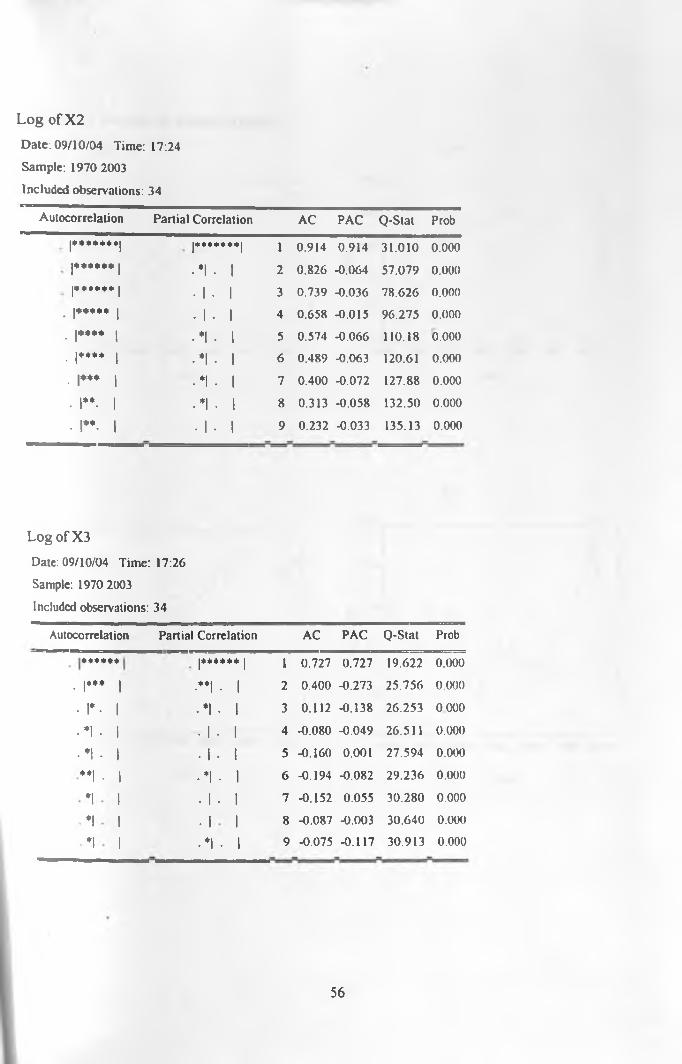
Log of X2

Date: 09/10/04 Time: 17:24 Sample: 1970 2003

Included observations: 34

Autocorrelation Partial Correlation AC PAC Q-Stat Prob|* + * * * + +| |** + * * * + | 1 0.914 0.914 31.010 0.000!♦ * ♦ * * * | • ♦I - 1 2 0.826 -0.064 57.079 0.000! * * » * * ♦ |

I I 3 0.739 -0.036 78.626 0.000

• .........1 • 1 • 1 4 0.658 -0.015 96.275 0.000

• ! * • • * 1 • *l . 1 5 0.574 -0.066 110.18 o.ooo

• ! * • • * 1 • 1 • 1 6 0.489 -0.063 120.61 0.000

• I* * * 1 • *l • 1 7 0.400 -0.072 127.88 0.000

• 1**- 1 ■ *l ■ 1 8 0.313 -0.058 132.50 0.000

• r - i • 1 ■ 1 9 0.232 -0.033 135.13 0.000

Log ofX3

Date: 09/10/04 Time: 17:26

Sample: 1970 2003

Included observations: 34

Autocorrelation Partial Correlation AC PAC Q-Stal Prob

| + t* + ** | 1 0.727 0.727 19.622 0.000

. I*** 1 •♦♦1 • 1 2 0.400 -0.273 25.756 0.000

• 1*. 1 • * l • 1 3 0.112 -0.138 26.253 0 000

• *1 • 1 • 1 • 1 4 -0.080 -0.049 26.511 0.000

• *1 • 1 • 1 • 1 5 -0.160 0.001 27.594 0.000

* * 1 . 1 •1-I 6 -0.194 -0.082 29.236 0.000

1 • 1 • 1 7 -0.152 0.055 30.280 0.000

1 •II 8 -0.087 -0.003 30.640 0.000

1 •*l • 1 9 -0.075 -0.117 30.913 0.000

56

Log

of x

2

1‘igure 1 Graphical Representation

(a) (b)

(c) (d)

57

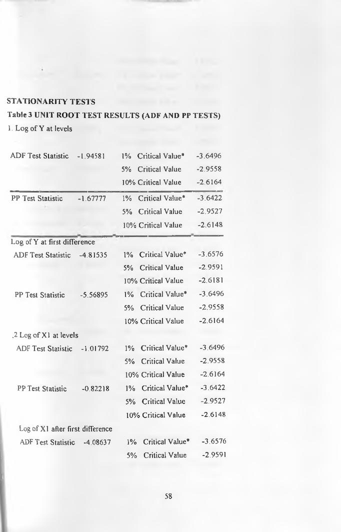
STATIONARITY TESTS

Table 3 UNIT ROOT TEST RESULTS (ADF AND PP TESTS)

1. Log of Y at levels

ADF Test Statistic -1.94581 1% Critical Value*

5% Critical Value

10% Critical Value

-3.6496

-2.9558

-2.6164

PP Test Statistic -1.67777 1% Critical Value* -3.6422

5% Critical Value -2.9527

10% Critical Value -2.6148

Log of Y at first difference

ADF Test Statistic -4.81535 1% Critical Value* -3.6576

5% Critical Value -2.9591

10% Critical Value -2.6181

PP Test Statistic -5.56895 1% Critical Value* -3.6496

5% Critical Value -2.9558

10% Critical Value -2.6164

.2 Log of XI at levels

ADF Test Statistic -1.01792 1% Critical Value* -3.6496

5% Critical Value -2.9558

10% Critical Value -2.6164

PP Test Statistic -0.82218 1% Critical Value* -3.6422

5% Critical Value -2.9527

10% Critical Value -2.6148

Log of XI after first difference

ADF Test Statistic -4.08637 1% Critical Value* -3.6576

5% Critical Value -2.9591

58

10% Critical Value -2.6181

PP Test Statistic -5.07000 1% Critical Value* -3.6496

5% Critical Value -2.9558

10% Critical Value -2.6164

3 Log of X2 at levels

ADF Test Statistic -2.22862 1% Critical Value* -3.6576

5% Critical Value -2.9591

10% Critical Value -2.6181

PP Test Statistic -2.62286 1% Critical Value* -3.6422

5% Critical Value -2.9527

10% Critical Value -2.6148

Log of X2 after first difference

ADF Test Statistic -3.36960 1% Critical Value* -3.6576

5% Critical Value -2.9591

10% Critical Value -2.6181

PP Test Statistic -4.73649 1% Critical Value* -3.6496

5% Critical Value -2.9558

10% Critical Value -2.6164

4 Log of X3 at levels

ADF Test Statistic -2.56505 1% Critical Value* -3.6496

5% Critical Value -2.9558

10% Critical Value -2.6164

PP Test Statistic -2.18109 1% Critical Value* -3.6422

5% Critical Value -2.9527

10% Critical Value -2.6148

Log of X3 after first difference

ADF Test Statistic -3 .24747 1% Critical Value* -3.6576

5% Critical Value -2.9591

10% Critical Value -2.6181

59

PP Test Statistic -4.39839 1% Critical Value* -3 6496

5% Critical Value -2.9558

10% Critical Value -2 6164

I able 5.4 Cointegration Analysis Results

ADF Test Statistic -3.655728 1% Critical Value* -3.6576

5% Critical Value -2.9591

10% Critical Value -2 6181

‘MacKinnon critical values for rejection of hypothesis of a unit root

Table 5.5 Correlation Matrixes

I.Y 1X1 I.X2 LX3________

LY 1 0.795422744 0.890922767 -0.108583827

LX1 0.795422744 1 0.062659222 0.114407772

LX2 0890922767 0.062659222 1 -0.020690933

LX3 -0.108583827 0.114407772 -0.020690933 1

60

Figure 6 Graph of Residuals

Residuals from the regression

61

Table 7. Regression Results (Long-Run Regression)

Dependent Variable: LY

Md: Least Squares

Date: 09/09/04 Time: 15:01

Sample: 1970 2003

Included observations: 34

Variable Coeflicien

t

Std. Error t-Statistic Prob.

LX1 0.216671 0.092705 2.337201 0.0271

LX2 1.088072 0.203808 5.338715 0.0000

LX3 0.376196 0.156719 2.400447 0.0235

LY1 0.044287 0.055766 0.794152 0.4340

D3 0.392696 0.111862 3.510524 0.0016

D2 0.238507 0.190698 1.250705 0.2218

C 0.420736 2.722781 0.154524 0.8783

R-squared 0.929412 Mean dependent var 14.92961

Adjusted R-squared 0.913725 S.D dependent var 0.417641

S.E. of regression 0.122672 Akaike info criterion -

1.177369

Sum squared resid 0.406305 Schwarz criterion -

0.863119

Log likelihood 27.01528 F-statistic 59.24991

Durbin-Watson stat 1.174223 Prob(F-statistic) 0.000000

62

Table 8 Regression Results (Differenced Model)

Dependent Variable: DLY

Method: Least Squares

Date: 09/10/04 Time: 14:42

Sample(adjusted): 1971 2003

Included observations: 33 after adjusting endpoints

Variable Coefficien

t

Std. Error t-Statistic Prob

DLX1 0.306958 0.148490 2.067194 0.0488

DLX2 0.760874 0.709399 2.072561 0.0033

DLX3 0.168273 0.220413 2.763446 0.0521

DLY1 -0.24802 0.190361 -1.302957 0.2040

D2 0.189767 0.169491 1.119633 0.2731

D3 0.206832 0.182407 2.133904 0.2672

c. 3.589019 2.735841 1.311852 0.2010

R-squared 0.737322 Mean dependent var 0.032232

Adjusted R-squared 0.61319 S.D. dependent var 0 142789

S.E. of regression 0.138342 Akaike info criterion -

0.932351

Sum squared resid 0.497598 Schwarz criterion -

0.614910

Log likelihood 22.38379 F-statistic 1.348401

Durbin-Watson stat 1.695895 Prob(F-statistic) 0.272093

63

Table 9 Regression Including Error Correction Model (ECM-1)Dependent Variable: DLY

Method: Least Squares

Date: 09/10/04 Time: 16:11

Sample(adjusted): 1972 2003

Included observations: 32 after .adjusting endpoints

Coefficient Std. Error t-Statistic Prob.

Variable

DLX1 -0.263314 0.151611 -1.736770 0.0952

DLX2 0.726712 0.752126 0.966210 0.3436

DLX3 0.168518 0.229702 0.733637 0.4703

D2 -0.023910 0.068668 -0.348197 0.7307

D3 -0.046958 0.081525 -0.576003 0.5700

DLY1 -0.042823 0.195602 -0.218928 0.8286

ECM_1 -0.289993 0.257010 -1.128336 0.2703

C 0.060933 0.074542 0.817435 0.4217

R-squared 0.266790 Mean dependent var 0.034744

Adjusted R-squared 0.052937 S.D. dependent var 0.144331

S.E. of regression 0.140459 Akaike info criterion -0.875490

Sum squared resid 0.473487 Schwarz criterion -0.509056

Log likelihood 22.00783 F-statistic 1.247537

Durbin-Watson stat 1.801931 Prob(F-statistic) 0.316862

64

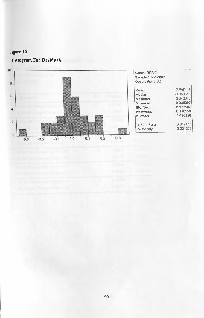
Histogram For Residuals

Figure 10

Series: RESIDSample 1972 2003Observations 32

Mean 7 59E-18Median -0.009510Maximum 0.342646Minimum -0.336007

Std Dev 0123587Skewness 0116556Kurtosis 4 486110

Jarque-Bera 3.017153

Probability 0 221225

65

Table 11 Pairwise Granger Causality Tests

Pairwise Granger Causality Tests

Date: 09/11/04 Time: 16:38

Sample: 1970 2003

Lags: 2

Null Hypothesis. Obs F-Statistic Probability

LX1 does not Granger Cause LY

LY does not Granger Cause LX1

32 0.47049

1.38413

0.62972

0.26776

LX2 does not Granger Cause LY

LY does not Granger Cause LX2

32 1.19229

3.01350

0.31901

0.06587

LX3 does not Granger Cause LY

LY does not Granger Cause LX3

32 0.003850.40318

0.99616

0.67215

LX2 does not Granger Cause LX1

LX1 docs not Granger Cause LX2

32 3.23695

0.12345

0.05494

0.88436

LX3 does not Granger Cause LX1

LX1 does not Granger Cause LX3

32 1.023950.19898

0.37270

0.82075

LX3 docs not Granger Cause LX2

LX2 docs not Granger Cause LX3

32 2.04449

0.18097

0.14901

0.83547

Figure (12)

Response to One S.D. Innovations ± 2 S E.

Response of LY to LY

Response of LX1 to LY Response of LX1 to LX1

Response of LX3 to LY Response of LX3 to LX1

Response of LX2 to LY Response of LX2 to LX1

Response of LY to LX3 Response of LY to LX2

Response of LX1 to LX3 Response of LX1 to LX2

Response of LX3 to LX3 Response of LX3 to LX2

Response of LX2 to LX3 Response of LX2 to LX/

67