factors controlling variability in the oxidative capacity ... · dell, 2001; young et al., 2013),...
TRANSCRIPT

Atmos. Chem. Phys., 14, 3589–3622, 2014www.atmos-chem-phys.net/14/3589/2014/doi:10.5194/acp-14-3589-2014© Author(s) 2014. CC Attribution 3.0 License.
Atmospheric Chemistry
and PhysicsO
pen Access
Factors controlling variability in the oxidative capacity of thetroposphere since the Last Glacial Maximum
L. T. Murray 1,*, L. J. Mickley 1, J. O. Kaplan2, E. D. Sofen3, M. Pfeiffer2, and B. Alexander3
1School of Engineering and Applied Sciences, Harvard University, Cambridge, MA, USA2ARVE Group, École Polytechnique Fédérale de Lausanne, Lausanne, Switzerland3Department of Atmospheric Sciences, University of Washington, Seattle, WA, USA* now at: Lamont-Doherty Earth Observatory, Columbia University, Palisades, NY, USA
Correspondence to:L. T. Murray ([email protected])
Received: 2 July 2013 – Published in Atmos. Chem. Phys. Discuss.: 17 September 2013Revised: 11 February 2014 – Accepted: 14 February 2014 – Published: 9 April 2014
Abstract. The oxidative capacity of past atmospheres ishighly uncertain. We present here a new climate–biosphere–chemistry modeling framework to determine oxidant levelsin the present and past troposphere. We use the GEOS-Chemchemical transport model driven by meteorological fieldsfrom the NASA Goddard Institute of Space Studies (GISS)ModelE, with land cover and fire emissions from dynamicglobal vegetation models. We present time-slice simulationsfor the present day, late preindustrial era (AD 1770), and theLast Glacial Maximum (LGM, 19–23 ka), and we test thesensitivity of model results to uncertainty in lightning andfire emissions. We find that most preindustrial and paleo cli-mate simulations yield reduced oxidant levels relative to thepresent day. Contrary to prior studies, tropospheric mean OHin our ensemble shows little change at the LGM relative tothe preindustrial era (0.5 ± 12 %), despite large reductionsin methane concentrations. We find a simple linear relation-ship between tropospheric mean ozone photolysis rates, wa-ter vapor, and total emissions of NOx and reactive carbonthat explains 72 % of the variability in global mean OH in 11different simulations across the last glacial–interglacial timeinterval and the industrial era. Key parameters controlling thetropospheric oxidative capacity over glacial–interglacial pe-riods include overhead stratospheric ozone, tropospheric wa-ter vapor, and lightning NOx emissions. Variability in globalmean OH since the LGM is insensitive to fire emissions. Oursimulations are broadly consistent with ice-core records of117O in sulfate and nitrate at the LGM, and CO, HCHO,and H2O2 in the preindustrial era. Our results imply thatthe glacial–interglacial changes in atmospheric methane ob-
served in ice cores are predominantly driven by changes inits sources as opposed to its sink with OH.
1 Introduction
The oxidative capacity of the troposphere – primarily char-acterized by the burden of the four most abundant and re-active oxidants (OH, ozone, H2O2, and NO3) – determinesthe lifetime before removal of many trace gases of impor-tance to climate and human health, including air pollutantsand the greenhouse gas methane (Fiore et al., 2012). Ozoneitself absorbs both longwave and shortwave radiation, andits tropospheric enhancement since the Industrial Revolutionis estimated to have contributed the third largest radiativeforcing effect of any gas over this period, after CO2 andmethane (IPCC, 2007). Oxidants also impact the evolution,lifetime, and physical properties of inorganic and primaryand secondary organic aerosol particles, modulating their di-rect and indirect radiative effects (Liao et al., 2003; Tie et al.,2005; Leibensperger et al., 2011). The tropospheric oxida-tive capacity may perturb terrestrial and marine ecosystemsvia oxidative stress and by altering deposition patterns of ox-idized nutrients such as nitrate (Shepon et al., 2007; Sitchet al., 2007; Collins et al., 2010). Understanding how tro-pospheric oxidative capacity has changed over the past iscritical for understanding its chemical, climatic, and eco-logical consequences. The oxidation capacity of past atmo-spheres, however, is uncertain. In this work, we introduce anew offline-coupled model framework to improve estimates
Published by Copernicus Publications on behalf of the European Geosciences Union.
3590 L. T. Murray et al.: Variability in tropospheric oxidants since the LGM
of the oxidative capacity on glacial–interglacial timescales,and we examine the implications of our results for currentunderstanding of the observed ice-core record of methane.
Tropospheric oxidant levels respond in well known butcomplex ways to meteorological conditions, changes inemissions of key chemical species, and changes in surfaceand stratospheric boundary conditions. These parameters in-clude temperature, clouds, water vapor concentrations, over-head ozone columns, aerosols, and emissions of reactive ox-ides of nitrogen (NOx), carbon monoxide, and volatile or-ganic compounds (VOCs) such as methane (e.g.,Thomp-son and Stewart, 1991; Spivakovsky et al., 2000; Lelieveldet al., 2002; Holmes et al., 2013). This sensitivity suggeststhat multi-millennial global environmental change, includingchanges in climate and land cover, should affect troposphericoxidative capacity.
Direct measurement of atmospheric oxidants is difficult atpresent, and nearly impossible for the past because most oxi-dants are highly reactive. The limited historical observationsof oxidant abundance that do exist imply that human activ-ity has indeed substantially perturbed the tropospheric oxi-dants since the preindustrial era (hereafter referred to as thepreindustrial) (e.g.,Staffelbach et al., 1991; Marenco et al.,1994; Anklin and Bales, 1997). The Last Glacial Maximum(LGM, 19–23 ka) is well characterized by ice-core and sedi-ment records, but no oxidants except for H2O2 are preservedin ice cores, and the H2O2 record is complicated by post-depositional processes (Hutterli et al., 2003). Proxies for ox-idant levels have been proposed, such as those from HCHOand methane (Staffelbach et al., 1991) or oxygen isotopeanomalies in sulfate and nitrate (e.g.,Alexander et al., 2002,2004; Kunasek et al., 2008), but these require models for in-terpretation in a global context. For methane, for example,there remains considerable uncertainty regarding the relativecontributions of the wetland emissions source vs. the OHsink in driving the large glacial–interglacial variability seenin ice-core bubbles (Khalil and Rasmussen, 1987; Chappel-laz et al., 1993; Crutzen and Brühl, 1993; Chappellaz et al.,1997; Martinerie et al., 1995; Brook et al., 2000; Kaplan,2002; Kaplan et al., 2006; Valdes et al., 2005; Levine et al.,2011c; Weber et al., 2010; Fischer et al., 2008; Singarayeret al., 2011; Levine et al., 2012).
Prior modeling studies that investigated past changes in thetropospheric oxidants have disagreed on the magnitude andeven the sign of changes, as summarized in Table1. Thesediscrepancies reflect differences in the model components ofthe Earth system allowed to vary, the differing degrees ofcomplexity in the representation of those components, andthe large uncertainties in past meteorological and biologi-cal conditions. Contributing to the uncertainty in estimatesof past oxidative capacity is the fact that the principal ox-idants are strongly and nonlinearly coupled to one another(Thompson, 1992). Models agree on the sign of the changein the global tropospheric mean ozone since the preindus-trial, with estimates of the change ranging from 25 to 65 %
(Wang and Jacob, 1998; Lelieveld and Dentener, 2000; Shin-dell, 2001; Young et al., 2013), but they have been unableto reproduce low surface concentrations of ozone implied bylate-19th-century observations (Marenco et al., 1994; Pavelinet al., 1999; Mickley et al., 2001). How OH changed over thisperiod is even more uncertain, with recent simulations from16 state-of-the-science models of the Atmospheric Chem-istry and Climate Model Intercomparison Project (ACCMIP)finding a mean change of−0.6± 8.8 % from 1850 to 2000,even with identical anthropogenic emission inventories ap-plied (Naik et al., 2013).
At the LGM, previous studies have generally found 20–30 % decreases in surface or free tropospheric ozone relativeto the preindustrial (Valdes et al., 2005; Kaplan et al., 2006;Karol et al., 1995). Most prior model studies have concludedthat OH concentrations at the LGM were about 25 % higherthan the preindustrial (range of 10–56 %) because of lowerhydrocarbon and CO concentrations (Law and Pyle, 1991;Crutzen and Zimmermann, 1991; Pinto and Khalil, 1991;Lu and Khalil, 1991; Martinerie et al., 1995; Valdes et al.,2005; Kaplan et al., 2006; Thompson et al., 1993, , and refer-ences therein), although the 1-D simulations byKarol et al.(1995) on average found 25 % less OH at the surface. How-ever, no LGM model study to date has considered the fullsuite of changes in the key variables for controlling tropo-spheric oxidants in a 3-D framework, in particular the ef-fect of the stratospheric ozone burden on photolysis rates inthe troposphere, to which OH is especially sensitive (e.g.,Holmes et al., 2013).
This study introduces the ICE age Chemistry And Prox-ies (ICECAP) project, which adopts as its central compo-nent a stepwise, offline-coupled framework for simulatingthe chemical composition of the atmosphere at and since theLGM. Our primary goal is to test, in a 3-D model, the sen-sitivity of tropospheric oxidants across the range of uncer-tainty in their controlling factors, with as much internal con-sistency as possible. Offline coupling, as opposed to usingan integrated Earth system model, allows for rapid sensitiv-ity tests and facilitates identification of first-order effects. Tothat end, we use a general circulation model (GCM) to sim-ulate meteorology for four different time slices: the presentday (ca. 1990s), the late preindustrial (ca. 1770s), and twodifferent possible representations of the LGM (19–23 ka),one significantly colder than the other to span the range oflikely LGM conditions. Second, we use the simulated me-teorology to determine land cover with an equilibrium ter-restrial biosphere model. We then apply the archived me-teorology and land cover products to a detailed chemicaltransport model (CTM), using an online-coupled linearizedstratospheric chemistry scheme for upper-boundary condi-tions. We allow tropospheric emissions of trace gases andaerosols to respond to climate within the CTM, and test thesensitivity of our results to two large sources of uncertainty:lightning and fires.
Atmos. Chem. Phys., 14, 3589–3622, 2014 www.atmos-chem-phys.net/14/3589/2014/

L. T. Murray et al.: Variability in tropospheric oxidants since the LGM 3591
Table 1.Percentage changes in tropospheric burdens of OH, ozone and H2O2, relative to the preindustrial, compiled from the literature
%1 at LGM %1 at present day
Reference OH Ozone OH Ozone H2O2 Method
McElroy (1989) +56 % – +60 % – – 1-D modelHough and Derwent(1990) – – −19 % – – 2-D modelValentin(1990) +23 % 0 % −9 % +64 % – 2-D modelLaw and Pyle(1991) – – −13 % +300 % – 2-D modelPinto and Khalil(1991), Lu and Khalil(1991) +15 %,+26 % −17 % −4 % +57 % – 1-D model, multi 1-D modelStaffelbach et al.(1991) – – −23 % – – Ice-core HCHOCrutzen and Zimmermann(1991) – – −10 % to−20 % +50 % – 3-D modelThompson et al.(1993) +10 % −20 % −17 % +80 % – Multi 1-D modelMartinerie et al.(1995) +20 % −30 % to+30 %a
+6 % Up to+250 %a – 2-D modelKarol et al.(1995) −60 % to+14 %b
−29 % to+12 %b+9 % to+12 %b
+56 % to+73 %b – Multi 1-D modelLevy et al.(1997) – – – +39 % – 3-D modelBerntsen et al.(1997) – – +6.80 % +53 % +100 % 3-D modelRoelofs et al.(1997) – – −22 % +43 % – 3-D modelBrasseur et al.(1998) – – −17 % +20 % to +80 %a – 3-D modelWang and Jacob(1998) – – −9.60 % +63 % – 3-D modelMickley et al.(1999) – – −16 % +56 % – 3-D modelLelieveld and Dentener(2000) – – – +25 % – 3-D modelGrenfell et al.(2001) – – −3.90 % +38 % – 3-D model, no NMVOCsHauglustaine and Brasseur(2001) – – −31 % +57 % – 3-D modelShindell et al.(2001) – – −5.90 % +45 % – 3-D modelLelieveld et al.(2002) – – −5 % +30 % – 3-D modelLamarque et al.(2005) – – −8 % +30 % – 3-D modelValdes et al.(2005) +25 %b
−17 %b – – – 3-D modelKaplan et al.(2006) +28 % −31 % – – – 3-D modelShindell et al.(2006) – – −16 % +11 % – 3-D modelSofen et al.(2011) – – −10 % +42 % +58 % 3-D modelParrella et al.(2012) – – – +47 % to+48 % – 3-D modelBock et al.(2012) +14 % – – – – 2-D modelNaik et al.(2013), Young et al.(2013) – – −0.6± 8.8 % +41± 8.9 % – Multi 3-D modelThis work, ensemble estimatec
+0.5± 12 % −20± 9 % +7.0± 4.3 % +28± 11 % +18± 22 % Multi 3-D modelThis work, best estimatec
+1.7 % −20 % +5.30 % +35 % +31 % 3-D modela Represents range throughout troposphere of local percentage changes relative to preindustrial, not a range in the global mean.b Difference reported for mean surface concentration.c cf. Sect.5 for description of ensemble and best estimates.
This paper focuses on the tropospheric gas-phase chem-istry component of the ICECAP project. In a separate paper,we will evaluate and interpret the role of aerosol particles oncomposition and climate across glacial–interglacial periods.
Section2 describes the climate, chemistry, and land mod-els used, and the manner in which they have been coupledto one another. Section3 summarizes and evaluates the fourdifferent climate simulations, focusing on the changes thatare most significant for tropospheric chemistry. Section4 de-scribes the response of natural emissions to changing climateas well as the scenarios we employ to test the sensitivity touncertainties in past lightning and fire emissions. Section5presents the resulting changes in tropospheric oxidants andidentifies their controlling factors, with particular focus onOH. Section6 evaluates and discusses the model results inthe context of the ice-core record. Section7 discusses the im-plications of our results for the methane record. We concludewith a summary section.
2 Methods: project and model description
Figure1 illustrates the stepwise offline coupling of the ICE-CAP project framework. Archived meteorology for multi-ple time slices from the NASA Goddard Institute of SpaceStudies (GISS) ModelE GCM (Schmidt et al., 2006) are
applied to the global vegetation models BIOME4-TG (Ka-plan et al., 2006) to determine land cover characteristics andLPJ-LMfire (Pfeiffer et al., 2013) to calculate dry matter con-sumed by fires. The archived meteorology and land coverproducts are then used to drive the GEOS-Chem CTM oftropospheric composition (Bey et al., 2001), which includesonline linearized stratospheric chemistry (McLinden et al.,2000).
2.1 The GISS ModelE general circulation model
The ModelE version of the GISS GCM of global climateis described in detail bySchmidt et al.(2006). The GISSGCM has a long history in investigations of past atmospheres(e.g.,Webb et al., 1997; Joussaume et al., 1999; Delaygueet al., 2000; Shindell et al., 2003; Schmidt and Shindell,2003; LeGrande et al., 2006; Rind et al., 2001, 2009). Weuse here ModelE with 4◦ latitude× 5◦ longitude horizon-tal resolution and 23 vertical layers extending from the sur-face to 0.002 hPa. We archive mean meteorological fieldsfrom ModelE for input to GEOS-Chem at temporal reso-lution of 6 h for three-dimensional fields (e.g., winds, con-vective mass fluxes) and 3 h for mixing depths and sur-face fields (e.g., surface temperature, solar radiation, albedo).The horizontal resolution used here is relatively coarse butstill common for simulations of global chemistry models
www.atmos-chem-phys.net/14/3589/2014/ Atmos. Chem. Phys., 14, 3589–3622, 2014

3592 L. T. Murray et al.: Variability in tropospheric oxidants since the LGM
26 Murray et al.: Variability in tropospheric oxidants since the LGM
ClimateGISS
ModelE GCM
(Schmidt et al., 2006)
Ice Core Records
VegetationBIOME4-TG
(Kaplan et al., 2006)
FireLPJ-LMfire
(Pfeiffer et al., 2013)
Tropospheric chemistryGEOS-Chem 3D CTM
(http://www.geos-chem.org)
Stratospheric chemistryLinoz
(McLinden et al., 2000)Isotope
chemistryGEOS-Chem
17O CTM(Sofen et al., 2011)
This study
Future study
Fig. 1. The ICE age Chemistry And Proxies (ICECAP) framework. Each box represents a separate model or measurement, except forstratospheric and tropospheric chemistry, which are online together in GEOS-Chem. Arrows indicate the coupling between models andmeasurements as used in this study. Dashed arrows indicate future work.
Fig. 1.The ICE age Chemistry And Proxies (ICECAP) framework.Each box represents a separate model or measurement, except forstratospheric and tropospheric chemistry, which are online togetherin GEOS-Chem. Arrows indicate the coupling between models andmeasurements as used in this study. Dashed arrows indicate futurework.
(e.g.,Lamarque et al., 2013). Climate in ModelE is forced bydifferent greenhouse gas levels from ice-core measurements,orbital parameters, topography, and fixed sea ice and sea sur-face temperatures (SSTs) as summarized in Table2 and dis-cussed in Sect.3. For each scenario the GCM is initialized forfive years, with four subsequent years of meteorology thenarchived for the terrestrial vegetation and chemical transportmodels. We discuss the forcings applied to the GISS climatemodel for each of the scenarios and the resulting climate inSect.3.1.
2.2 The BIOME4-TG global vegetation model
BIOME4-TG (Kaplan et al., 2006) is an equilibrium ter-restrial vegetation model that calculates the global distribu-tion of 28 biomes and a suite of associated biogeochemi-cal state variables and fluxes. The model is driven by cli-matological mean monthly climate, soil texture in two lay-ers, and atmospheric CO2 concentrations. BIOME4-TG hasbeen used extensively for simulating past vegetation dis-tributions and for evaluating paleoclimate simulations fromGCMs against paleoecological archives (e.g.,Kaplan, 2002;Kaplan et al., 2003, 2006; Harrison and Prentice, 2003). Forthis study, we drive BIOME4-TG with a standard baselineclimatology (Kaplan et al., 2006) to which we add monthlymean anomalies of surface temperature, precipitation, andsolar radiation from the GISS ModelE paleo and preindus-trial climate scenarios. The BIOME4-TG outputs passed toGEOS-Chem are biome classification and each biome’s con-stituent plant functional types (PFTs), as well as aggregateleaf area index (LAI). The PFTs and LAI are used for deter-mining terrestrial plant emissions of VOCs (Sect.4.2); LAIand biome classes are used in calculating dry deposition ve-locities in a resistance-in-series model in GEOS-Chem (We-sely, 1989). We elect to represent present-day land cover withBIOME4-TG rather than prescribe it from satellite products(as normal for GEOS-Chem) for consistency between simu-lations. However, to represent anthropogenic land use, we su-
perimpose a present-day crop fraction mask from the Modelof Emissions of Gases and Aerosols from Nature (MEGAN)version 2.1 (Guenther et al., 2012).
2.3 The LPJ-LMfire global biomass burning model
LPJ-LMfire (Pfeiffer et al., 2013) is a dynamic global vege-tation model designed to simulate biomass burning from nat-ural and human-caused wildfires in preindustrial time. Themodel further accounts for intentional burning of agricul-tural land and pastures in preindustrial societies. Similarly toBIOME4-TG, we drive LPJ-LMfire with a standard baselineclimatology (Pfeiffer et al., 2013) to which we add monthlymean anomalies of mean temperature, diurnal temperaturerange, precipitation, total cloud cover fraction, surface andwind speed from the GISS ModelE scenarios. Monthlyanomalies of lightning ground-strike rate determined byGEOS-Chem (Sect.4.5) are also used to drive LPJ-LMfirein the paleoclimate experiments. We archive monthly totaldry mass of biomass burned for use in GEOS-Chem.
2.4 The GEOS-Chem chemical transport model
The GEOS-Chem global CTM (version 9-01-03, with modi-fications as described;http://www.geos-chem.org) simulatestropospheric ozone–NOx–CO–VOC–BrOx–aerosol chem-istry. Emissions and their coupling with the GCM and veg-etation model outputs are the subject of Sect.4. The origi-nal description of the chemical mechanism is byBey et al.(2001). The coupled sulfur–nitrate–ammonium aerosol sim-ulation is described byPark et al.(2004), with aerosol ther-modynamics computed via the ISORROPIA II model (Foun-toukis and Nenes, 2007) as implemented byPye et al.(2009).Sea salt aerosol is described byJaeglé et al.(2011), primaryand secondary organic aerosol byHeald et al.(2011), andblack carbon byWang et al.(2011). Recent updates of rel-evance for this study include those to oceanic sources andsinks of acetone (Fischer et al., 2012), optical properties ofdust (Ridley et al., 2012), and snow scavenging and washoutof aerosols (Wang et al., 2011). We include online brominechemistry (Parrella et al., 2012), whose catalytic destructionof ozone may be an important mechanism for limiting prein-dustrial ozone levels.
In their study of effect of climate change on surfaceair quality in the near future,Wu et al. (2007) coupledGEOS-Chem with the GISS III version of the GISS GCM(Rind et al., 2007). Here, we build upon theWu et al.(2007)framework, using meteorology from GISS ModelE to driveGEOS-Chem chemistry. Primary differences between theWu et al.(2007) implementation and this work include theprescription of land cover from an offline global terrestrialvegetation model (Sects.2.2–2.3and4.2), a linearized strato-spheric ozone scheme, adjusted convective transport andrainout schemes to reflect the updated moist convection inModelE (Kim et al., 2012), and implementation of the GISS
Atmos. Chem. Phys., 14, 3589–3622, 2014 www.atmos-chem-phys.net/14/3589/2014/

L. T. Murray et al.: Variability in tropospheric oxidants since the LGM 3593
Table 2.Climate forcings used in GISS ModelE for each climate scenario.
Simulation parametersLast Glacial Maximum (21 ka) Preindustrial Present day
Cold LGM Warm LGM (ca. 1770s) (ca. 1990s)
Greenhouse gases (ppmv)CO2 188 188 280 354N2O 0.20 0.20 0.27 0.31CH4 0.39 0.39 0.73 1.69CFCs 0 0 0 1990 values
SST and sea ice Webb et al.(1997) CLIMAP (1976)1880s 1990s
Rayner et al.(2003) Rayner et al.(2003)Ice sheet topography Licciardi et al.(1998) Licciardi et al.(1998) Present day Present dayStratospheric ozonea 1880s values 1880s values 1880s values 1990s valuesOrbital forcingb 2000 conditionsc 2000 conditionsc 1770 conditions 2000 conditionsTropospheric aerosols and ozoned 1880s values 1880s values 1880s values 1990s values
a As used byHansen et al.(2007). b Calculation fromBerger(1978). c Orbital parameters for the LGM are nearly the same as they are today (Braconnot et al., 2007a).d Aerosols fromKoch et al.(2009). Ozone fromShindell et al.(2008).
quadratic upstream tracer advection scheme (Prather, 1986)for improved consistency with the GCM. We discuss theseupdates in detail below.
For this work, we prescribe atmospheric methane con-centrations, imposing a meridional gradient as summarizedin Table3. The preindustrial and LGM simulations use ob-served methane values from Antarctic, Andean, and Green-land ice cores in the NOAA National Geophysical DataCenter (NGDC) Paleoclimatology Program (http://www.ncdc.noaa.gov/paleo/paleo.html) (Chappellaz et al., 1990;Etheridge et al., 1998; Blunier et al., 1998; Thompson, 1998;Petit et al., 1999; Campen, 2000; Loulergue et al., 2008). Ourpresent-day values are from flask observations of the NOAAGlobal Monitoring Division database (http://www.esrl.noaa.gov/gmd/) (Dlugokencky et al., 2008). We assume methaneis uniformly mixed up to the tropopause in each latitudinalband. In the present day and preindustrial, methane increaseswith increasing latitude in the Northern Hemisphere, reflect-ing its terrestrial source. The record of tropical methane ex-ists from a single ice core and implies that tropical methaneat the LGM maintained preindustrial levels. This ice corewas likely contaminated by in situ methanogenic production(Campen et al., 2003), and it is unlikely that a gas with achemical lifetime of 10 years could maintain such a largetropical–extratropical gradient. We therefore assume tropicalmethane to be 4 % higher than recorded for Antarctica. Thisis similar to the present-day gradient, and consistent with ear-lier model studies of LGM methane (Kaplan et al., 2006) andwetland emissions (Weber et al., 2010).
We calculate stratospheric ozone online in GEOS-Chemfollowing the Linoz linearized chemical scheme (McLin-den et al., 2000), with coefficients appropriate for strato-spheric chemistry in the LGM (Rind et al., 2009) and thepreindustrial (C. McLinden, personal communication, 2009).GEOS-Chem typically uses satellite observations of total
Table 3.Methane mixing ratios prescribed in GEOS-Chem [ppbv].
90–30◦S 30◦S–0◦ 0◦–30◦N 30–90◦N
Present daya 1690 1700 1760 1810Preindustrialb 710 725 725 760LGMb 370 385 385 375
a Present-day values from flask samples of the NOAA Global Monitoring Division(GMD) database.b Preindustrial and LGM are mean values from ice-core records inthe NOAA National Geophysical Data Center (NGDC) Paleoclimatology Program,except for the tropical LGM, which is assumed to be 4 % higher than Antarcticmethane.
ozone columns to determine the attenuation of shortwave ra-diation in its calculation of tropospheric photolysis rates. Ouruse of Linoz allows for calculation of photolysis rates moreconsistent with changing climate and chemical conditions.
In addition to ozone, we also calculate an array of 20+other species in the stratosphere to account for chemi-cal fluxes across the tropopause. For example, the strato-sphere is a net source of NOx into the troposphere anda net sink of tropospheric CO. Stratospheric concentra-tions of these species are calculated from monthly cli-matological 3-D production rates and loss frequenciesarchived from the Global Modeling Initiative (GMI) CTMdriven by MERRA assimilated meteorology for 2004–2010(Allen et al., 2010; Duncan et al., 2007; Considine et al.,2008) and re-gridded to the ModelE grid. We approxi-mate the paleo-stratosphere by scaling the production ratesof NOx and HNO3 by the ratio of the primary strato-spheric nitrogen precursor (N2O) observed in NOAA/NGDCice cores (preindustrial/present= 0.83; LGM/present= 0.77)(Fluckiger et al., 2002), and similarly for CO by theratio of ice-core methane (preindustrial/present= 0.41;LGM/present= 0.32). Bromine species are the exception tothe linearized treatment, and stratospheric concentrations are
www.atmos-chem-phys.net/14/3589/2014/ Atmos. Chem. Phys., 14, 3589–3622, 2014

3594 L. T. Murray et al.: Variability in tropospheric oxidants since the LGM
instead prescribed as described byParrella et al.(2012) anddo not change between climates.
To reach equilibrium with respect to stratosphere–troposphere exchange, each scenario was initialized over10 years, repeatedly using the first year of archived meteorol-ogy. Simulations for analysis use the three remaining years ineach climate scenario.
2.5 Evaluation of present-day simulation
We evaluate the ICECAP present-day simulation against asuite of sonde, aircraft, satellite, and surface measurementsof trace gases, aerosols, and radionuclides, and we also com-pare ICECAP with the standard GEOS-Chem driven by as-similated meteorology (GEOS4 and GEOS5). We refer thereader to the supplemental materials for the details, and sum-marize here. Tropospheric vertical mixing performs betterthan, or on par with, the GEOS simulations as inferred bycomparisons to observed vertical profiles of222Rn and sur-face ratios of7Be /210Pb. Stratospheric age of air reaches 4–5 years by 35 km in our simulations, 1–2 years longer thaneither GEOS simulation, but in better agreement with ob-servations (Waugh and Hall, 2002). We find a troposphericresidence time for210Pb-containing aerosols against deposi-tion of 7.2 d, within the range of previous model studies: 6.5–12.5 d (Turekian et al., 1977; Lambert et al., 1982; Balkanskiet al., 1993; Koch et al., 1996; Guelle et al., 1998a, b; Liuet al., 2001).
Our simulated methyl chloroform (CH3CCl3) lifetimeagainst loss from tropospheric OH is 5.5 years, which is closeto the 6.0+0.5
−0.4 years inferred from observations byPrinn et al.(2005), and comparable to recent multi-model estimates of5.7 ± 0.9 years (Naik et al., 2013). The methane lifetimeagainst tropospheric OH is 10.4 years (cf. Sect.7), whichmatches the best estimate of 10.2+0.9
−0.7 years fromPrinn et al.(2005), recent multi-model estimates of 10.2± 1.7 (Fioreet al., 2009) and 9.8± 1.6 years (Voulgarakis et al., 2013),and an observationally derived estimate of 11.2± 1.3 years(Prather et al., 2012).
The simulated present-day stratospheric columns of ozone(SCO) in our model have a small mean bias of+1.5 % vs. a2004–2010 climatology from satellite (Ziemke et al., 2011).However, we overestimate SCO over the poles by 5–50 %due to an overly vigorous Brewer–Dobson circulation, partic-ularly over Antarctica during austral spring (> 100 %) as ourimplementation of Linoz does not include the heterogeneousreactions of the ozone hole. In the troposphere, we underesti-mate tropical ozone columns by 20 % and overestimate extra-tropical columns by 45 % vs. satellite climatologies (Ziemkeet al., 2011). Comparison with ozonesondes indicates thatthe tropical bias is in the free- and upper troposphere andnot at the surface, and that the extratropical bias is a spring-time feature in both hemispheres, consistent with overesti-mated transport from the stratosphere. Overly vigorous massfluxes from the stratosphere to the troposphere have histor-
ically been a problem with CTMs (e.g.,Liu et al., 2001),and some models have prescribed cross-tropopause fluxes ofozone (e.g.,Wu et al., 2007). Here we elect to accept thebias in the cross-tropopause flux of ozone in the present dayin order to examine the role of the tropical overhead ozonecolumns on photolysis in different climates. The extratropi-cal biases in ozone will have relatively little impact on theglobal budget of OH, whose burden is primarily in the tropi-cal lower free troposphere (Spivakovsky et al., 2000).
3 Climate
3.1 Climate forcings
Table2 summarizes the different greenhouse gas levels, or-bital parameters, topography, and fixed sea ice and sea sur-face temperatures (SSTs) used to force each of our four sim-ulations. In this section and throughout the paper, we reportmost changes relative to the state of the preindustrial.
Simulations of LGM climate are sensitive to assumptionsabout ice sheet topography and tropical SSTs (Rind, 2009),and these assumptions have implications for the chemi-cal composition of the troposphere, as they affect trans-port, surface emissions, and the surface UV albedo. At theLGM, large permanent land ice sheets 3–4 km thick existedover northern North America (Laurentide and Cordilleran),Greenland, and northwestern Eurasia (Fennoscandian). Weuse here the reconstruction of ice sheet thickness and extentfrom Licciardi et al. (1998), which has a lower maximumLaurentide Ice Sheet (LIS) elevation than those in the Pale-oclimate Modelling Intercomparison Project (PMIP) studies(Braconnot et al., 2007a, 2012). Ullman et al.(2013) evalu-ated the sensitivity of the resulting LGM climate in ModelEto two different ice-sheet reconstructions, includingLicciardiet al. (1998). They concluded that the lower maximum LISelevation led to cooler temperatures in the northern latitudes.The accumulation of water in terrestrial ice sheets causedsea levels to drop 120 m, exposing an additional 3 % of theEarth’s surface as land, particularly in Southeast Asia andOceania, the Bering Strait, and the southeastern continentalshelf of South America (Clark and Mix, 2002).
Figure2 shows the annual mean SST distribution used ineach past simulation. SSTs in the preindustrial and present-day simulations are from the Hadley Centre sea ice and SSTversion 1 (HadISST1) data set (Rayner et al., 2003). Forthe LGM, large uncertainty exists over the extent of cool-ing of tropical SSTs, which strongly affects LGM dynam-ics because of its influence on meridional temperature gra-dients and low-latitude circulation (Rind, 2009). To boundthe range of likely conditions, we simulate two potential re-alizations of the LGM climate driven by different SSTs. Forour “warm-LGM” simulation, we use the SST reconstruc-tion from the “Climate: Long range Investigation, Mapping,and Prediction” project (CLIMAP, 1976), with an average
Atmos. Chem. Phys., 14, 3589–3622, 2014 www.atmos-chem-phys.net/14/3589/2014/

L. T. Murray et al.: Variability in tropospheric oxidants since the LGM 3595
Murray et al.: Variability in tropospheric oxidants since the LGM 27
Fig. 2. Top panel shows preindustrial sea surface temperature (SST), as reconstructed by proxies (Rayner et al., 2003). Bottom two panels arethe absolute changes in SST during the warm-LGM (bottom left; CLIMAP, 1976) and cold-LGM (bottom right; Webb et al., 1997) scenarios,relative to the preindustrial, with the LGM coastlines and ice sheets. The difference plots share a common colorbar. The change in SST fromthe preindustrial to the present day is relatively small (not shown).
Fig. 2. Top panel shows preindustrial sea surface temperature(SST), as reconstructed by proxies (Rayner et al., 2003). Bottomtwo panels are the absolute changes in SST during the warm LGM(bottom left;CLIMAP, 1976) and cold LGM (bottom right;Webbet al., 1997) scenarios, relative to the preindustrial, with the LGMcoastlines and ice sheets. The difference plots share a common colorbar. The change in SST from the preindustrial to the present day isrelatively small (not shown).
change in SST within 15◦ of the Equator (1SST15◦ S−15◦ N)of −1.2◦C. The CLIMAP reconstruction indicates that muchof the subtropical Pacific was warmer in the LGM than inthe preindustrial, a controversial result (e.g.,Rind and Pe-teet, 1985). For our “cold-LGM” simulation, we use SSTsfrom Webb et al.(1997), who achieved1SST15◦ S−15◦ N of−6.1◦C by imposing an ocean heat transport flux in the GISSGCM. The recent “Multiproxy Approach for the Reconstruc-tion of the Glacial Ocean surface” project (MARGO ProjectMembers, 2009) concluded that the SST change was likelycolder than that implied by the CLIMAP reconstruction(1SST15◦ S−15◦ N =−1.7◦C) with a more subdued warmingof the subtropical Pacific gyres, but not as cold as inWebbet al. (1997). These changes at the LGM are all greater inmagnitude than the present-day1SST15◦ S−15◦ N of +0.4◦Crelative to the preindustrial.
3.2 Climate results
Table 4 shows mean values for the globe and large zonalbands of meteorological variables in each simulated cli-mate scenario. Relative to the preindustrial, surface air tem-peratures are 1.4 and 6.8◦C colder in the warm-LGM andcold-LGM scenarios, respectively, driven by the decreases ingreenhouse gases and SSTs and the increase in topography(Fig. 3, left column). The changes in surface temperature tothe LGM are much greater in magnitude than the simulated0.5◦C increase from the preindustrial to the present day (notshown). Tropospheric water vapor is highly sensitive to tem-perature (e.g.,Held and Soden, 2006; Sherwood et al., 2010),and tropical specific humidity in our warm-LGM and cold-LGM scenarios decrease by 10 and 38 % relative to the prein-dustrial.
Figure3 also shows the changing distribution of precip-itation in each past scenario (right column). The decreasesin greenhouse gases and water vapor increase the tropicaltropospheric lapse rate at the LGM, reducing the depth andintensity of tropical deep convection (e.g.,Sherwood et al.,2010) and weakening the Hadley circulation. With reducedupwelling near the Equator, precipitation decreases in thetropics and increases in the subtropics, especially in the warmpools in the CLIMAP reconstruction.
The residual circulation of the stratosphere also weakenswith decreasing levels of greenhouse gases in our simula-tions. Stratospheric circulation is characterized by net ascentin the tropics and descent in the extratropics, driven by strato-spheric breaking of upward-propagating planetary waves oftropospheric midlatitude origin (Holton et al., 1995). Thevertical component of the residual circulation (w∗) weak-ens in magnitude relative to the preindustrial by an averageof 16 and 32 %, respectively, in the warm-LGM and cold-LGM scenarios at 50 hPa in the tropics (12◦ S–12◦ N), andincreases by 5 % in the present day. There are correspondingchanges in the extratropics. The mass-weighted mean strato-spheric age of air (Waugh and Hall, 2002) deduced from anSF6-like tracer in GEOS-Chem is 9–15 % greater in the LGMthan the preindustrial, consistent with the weakening residualcirculation; the present-day age of air is 8 % lower than thepreindustrial.
That the strength of the residual circulation is correlatedwith greenhouse gas levels is a robust result of GCMs (Gar-cia and Randel, 2008), including at the LGM (Rind et al.,2001, 2009), although not clearly supported by observations(Engel et al., 2008). The decreased thermal wind shear atthe LGM reduces the strength of the subtropical jet, whichin turn weakens wave penetration into the stratosphere andleads to deceleration of the residual circulation relative tothe preindustrial; the converse holds for the preindustrial topresent (Shepherd and McLandress, 2011). Weakened tropi-cal deep convection at the LGM and increased static stabilityabout the tropopause from stratospheric radiative warmingalso impedes mixing across the tropopause. In addition, thetropopause height decreases in each colder climate; in thecold-LGM scenario it is 2 km lower than in the preindustrial.The slowing of the residual circulation of the stratosphere to-gether with decreases in tropopause height during the LGMcontribute toward enhancement of the SCO and have impli-cations for photolysis rates in the tropical troposphere, as wedescribe in Sect.5.1.
3.3 Evaluation of simulated LGM climate
Figure4 demonstrates that our GISS ModelE climate simu-lations for the LGM are in broad agreement with other LGMmodel studies and an independent reconstruction of regionalLGM climate from pollen records. The left panels comparethe zonal mean temperature and precipitation changes of ourtwo LGM simulations to the mean and range of those values
www.atmos-chem-phys.net/14/3589/2014/ Atmos. Chem. Phys., 14, 3589–3622, 2014

3596 L. T. Murray et al.: Variability in tropospheric oxidants since the LGM
28 Murray et al.: Variability in tropospheric oxidants since the LGM
Fig. 3. Simulated surface air temperatures (left column; ◦C) and precipitation fluxes (right column; mm d−1). Top panels: Preindustrialconditions. Bottom panels, absolute change from preindustrial to warm-LGM (middle row; CLIMAP, 1976) and cold-LGM (bottom row;Webb et al., 1997) scenarios. Both difference plots share a common colorbar for each variable. The green dots indicate regions with significantchanges, as determined by a Student’s t-test with degrees of freedom adjusted for autocorrelation (Wilks, 2011). The changes relative to thepreindustrial in present-day surface temperatures and precipitation fluxes are small, and significant only at the poles and over small areas ofthe tropics, respectively (not shown).
Fig. 3. Simulated surface air temperatures (left column,◦C) and precipitation fluxes (right column, mm d−1). Top panels: preindustrialconditions. Bottom panels, absolute change from preindustrial to warm-LGM (middle row;CLIMAP, 1976) and cold-LGM (bottom row;Webb et al., 1997) scenarios. Both difference plots share a common color bar for each variable. The green dots indicate regions withsignificant changes, as determined by a Student’st test with degrees of freedom adjusted for autocorrelation (Wilks, 2011). The changesrelative to the preindustrial in present-day surface temperatures and precipitation fluxes are small, and significant only at the poles and oversmall areas of the tropics, respectively (not shown).
Table 4.Climate results for the four scenarios.
Last Glacial Maximum (21 ka)
Cold LGM Warm LGM Preindustrial Present daySimulated variablea G SH T NH G SH T NH G SH T NH G SH T NH
Surface air temperature [◦C] 6.1 −3.7 19.2 -2 10.7 1.5 24.6 0.8 14.3 5.4 26 7.4 14.9 6 26.5 8Specific humidity [g kg−1] 1.8 1.3 1.8 1.8 2.6 1.7 2.6 2.6 2.9 2 2.9 2.9 3 2.1 3 3Tropopause pressure [hPa] 151 196 98 180135 173 80 172 126 165 75 158 123 160 73 155Precipitation rate [mm d−1] 2.4 1.6 3.5 1.7 2.8 2 4.2 1.9 3 2.3 4.3 2.1 3 2.3 4.3 2.1Ground albedo [%] 21 29 9 28 20 26 9 30 14 18 8 20 14 17 8 19Land coverage [%] 33 17 27 56 33 17 27 56 29 16 24 47 29 16 24 47Land ice coverage [%] 7 9 0 16 7 9 0 16 3 9 0 2 3 9 0 2Ocean/lake ice coverage [%] 11 31 0 7 10 24 0 9 5 8 0 8 4 7 0 7Total cloud cover [%] 58 69 48 62 57 64 49 61 58 63 51 61 59 63 52 63Cloud top pressure [hPa] 616 667 579 616585 640 535 601 570 616 536 570 574 616 540 577Elevation above sea level [m] 341 271 170 646341 271 170 646 238 218 145 386 238 218 145 386Surface wind speed [m s−1] 5.5 6.9 5.1 4.5 5.4 7.1 4.8 4.5 5.3 6.9 4.7 4.7 5.3 6.9 4.7 4.7Stratospheric age of airb [years] 1.64 1.55 1.43 1.31
a Annual multi-year tropospheric mean values for the globe (G), Southern Hemisphere (SH, 90–23◦ S), tropics (T, 23◦ S–23◦ N), and Northern Hemisphere (NH, 23–90◦ N).b Mass-weighted mean stratospheric age of air (Waugh and Hall, 2002), calculated with anSF6-like inert tracer.
in the models participating in PMIP2 (Braconnot et al.,2007a, b). Each of the seven models that simulated the LGMfor PMIP2 had a fully coupled ocean–atmosphere, and didnot prescribe SSTs as we do here. Our LGM scenarios bound
the PMIP2 ensemble mean change of−2.3◦C in the tropicsrelative to the preindustrial. Our simulations find decreases inzonal mean precipitation of 10–50 % within 10◦ of the Equa-tor, and of 10–90 % within 40◦ of the poles, as well as little
Atmos. Chem. Phys., 14, 3589–3622, 2014 www.atmos-chem-phys.net/14/3589/2014/
L. T. Murray et al.: Variability in tropospheric oxidants since the LGM 3597
Murray et al.: Variability in tropospheric oxidants since the LGM 29
−30
−20
−10
0
10 Zonal mean
(a) Change from preindustrial in mean surface air temperature [oC]
Warm LGMCold LGM
Present DayPMIP2 Ensemble LGM
Regional
Warm LGMCold LGM
Pollen RecordPMIP2 Ensemble
−4
−3
−2
−1
0
1
2
3
90oS 40
oS 20
oS 0
o20
oN 40
oS 90
oN
(b) Change from preindustrial in mean precipitation flux [mm d−1
]
Alaska N. America Africa Eurasia
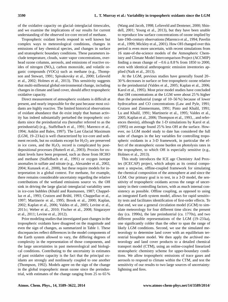
Fig. 4. Evaluation of climate changes for (a) mean surface temperature and (b) zonal mean precipitation flux. The left panels compare ourModelE simulations to the range of zonal mean changes from the preindustrial in the Paleoclimate Multimodelling Intercomparison ProjectPhase II (PMIP2; Braconnot et al., 2007a). The latitudinal axis is weighted by relative zonal area. The right panels compare our simulationto the pollen-based climate reconstruction from Bartlein et al. (2011) using box-and-whisker plots; dots indicate outliers. That study used thepresent day as its baseline, and we follow that convention here. We sample our simulations and the PMIP2 ensemble at the locations of thesediment core measurements.
Fig. 4. Evaluation of climate changes for(a) mean surface temperature and(b) zonal mean precipitation flux. The left panels compare ourModelE simulations to the range of zonal mean changes from the preindustrial in the Paleoclimate Multimodelling Intercomparison ProjectPhase II (PMIP2;Braconnot et al., 2007a). The latitudinal axis is weighted by relative zonal area. The right panels compare our simulation tothe pollen-based climate reconstruction fromBartlein et al.(2011) using box-and-whisker plots; dots indicate outliers. The above study usedthe present day as its baseline, and we follow that convention here. We sample our simulations and the PMIP2 ensemble at the locations ofthe sediment core measurements.
change in the midlatitudes as in the mean of the PMIP2 en-semble. Precipitation increases up to 25–33 % in the tropicspoleward of the Equator in our simulations, where the PMIP2ensemble mean is zero. Our zonal mean LGM precipitationchanges are of greater magnitude than the range of PMIP2.
Figure4 also compares our modeled results and those ofPMIP2 to an inverse reconstruction of regional climate usingpaleoecological archives byBartlein et al.(2011). Temper-ature changes in the warm-LGM simulation relative to thepreindustrial better match values inferred from the pollendata than do those in the cold-LGM simulation, with meanabsolute biases of 4.4 and 5.1◦C, respectively (the PMIP2bias is 3.5◦C). Both PMIP2 and our simulations have diffi-culty in matching the inferred changes in precipitation, ex-cept over Africa, where the cold LGM performs well. Thepollen record has a small sample size (n = 98 at the LGM)and a limited geographic distribution, but does provide someconfidence in our choice of LGM scenarios as brackets of arange of probable climates.
4 Tropospheric emissions
Figure5 summarizes the gas-phase emissions and Fig.6 thedirect and precursor aerosol emissions in our different sim-ulations. Wherever possible, emissions respond to changingmeteorology from the GCM, as described below. We test thesensitivity of our results to three different emission scenar-
ios in the preindustrial and LGM atmospheres: a low-fireand a high-fire scenario, which together span the range ofestimated past fire magnitudes (Sect.4.6), and a scenario inwhich we fix the total lightning source in all climates to com-pare to our other simulations in which total lightning changeswith climate (Sect.4.5).
4.1 Anthropogenic
Present-day anthropogenic emissions from fuel combustion,agriculture, and industry are prescribed from the Emis-sion Database for Global Atmospheric Research (EDGAR)base inventory for 2000 (Olivier, 2001), overwritten withregional inventories for the United States (EPA NEI99),Canada (CAC), Mexico (BRAVO;Kuhns et al., 2005), Eu-rope (EMEP;Auvray and Bey, 2005), and South and EastAsia (Streets et al., 2003, 2006). These inventories all havemonthly variability, some with additional weekly cycles.Biofuel emissions (Yevich and Logan, 2003) and aircraftemissions are constant. All emissions are scaled as describedby van Donkelaar et al.(2008) to 1995 values for our present-day simulation. Our preindustrial and LGM simulations as-sume no anthropogenic emissions aside from a small bio-fuel burning source in the preindustrial that is 45 % of thepresent-day value, estimated by scaling and distributing the1850 country-level inventory fromFernandes et al.(2007)by the grid cell level of population between 1770 and 1850
www.atmos-chem-phys.net/14/3589/2014/ Atmos. Chem. Phys., 14, 3589–3622, 2014

3598 L. T. Murray et al.: Variability in tropospheric oxidants since the LGM
30 Murray et al.: Variability in tropospheric oxidants since the LGM
Cold LGM
Warm LGM
Preind.
Cold LGM
Warm LGM
Preind.
Cold LGM
Warm LGM
Preind.
Present Day
0 10 20 30 40 50
6.3 3.7 10.5
6.3 6.1 13
6.3 4.9 6.2 1 18.3
3.3 12.6 3.7 19.6
4.8 12.5 6.1 23.4
6 20.7 6.2 1 33.9
3.3 3.7 7.5
4.8 6.1 11.4
6 4.9 6.2 1 18.1
6.3
Lightning
6.4
Fires
7.2
Soil
25.8
Fuel Combustion
45.7
(a) NOx Emissions [Tg N yr−1
]
fixed
lightning
high
fire
low
fire
Cold LGM
Warm LGM
Preind.
Cold LGM
Warm LGM
Preind.
Present Day
0 500 1000 1500 2000 2500
880 111 424 1415
903 157 689 1750
1482 304 800 2656
115 398 548
158 664 860
349 317 769 1504
453
Fires
805
Methane oxidation
687
NMVOC oxidation
412
Fuel Combustion
2357
(b) CO Sources (Direct Emissions + Chemical Production) [Tg yr−1
]
high
fire
low
fire
Cold LGM
Warm LGM
Preind.
Present Day
0 200 400 600 800
261 70 66 406
478 100 95 687
580 122 106 826
536
Isoprene
114
Monoterpenes
101
Acetone Other
767
(c) Terrestrial Plant VOC Emissions [Tg C yr−1
]
Fig. 5. Gas phase emissions used for each climate scenario. We test two different fire emission scenarios, a high fire scenario with pastfire emissions from the LPJ-LMfire model (Pfeiffer et al., 2013), and a low fire scenario in which we scale the model output by sedimentrecords of charcoal accumulation rates (Power et al., 2008). We also perform a fixed lightning suite of simulations in which we scale the totallightning NOx source to be constant in different climates.
Fig. 5.Gas-phase emissions used for each climate scenario. We testtwo different fire emission scenarios, a high-fire scenario with pastfire emissions from the LPJ-LMfire model (Pfeiffer et al., 2013),and a low-fire scenario in which we scale the model output by sed-iment records of charcoal accumulation rates (Power et al., 2008).We also perform a fixed lightning suite of simulations in which wescale the total lightning NOx source to be constant in different cli-mates.
from the History Database of Global Environment (HYDEv3.1; Klein Goldewijk et al., 2011). Anthropogenic emis-sions since the preindustrial yield large perturbations to thetropospheric budgets of reactive nitrogen, carbon, and sulfur(Fig. 5 and Fig.6), predominantly in the northern midlati-tudes.
4.2 Biogenic – land
Terrestrial plant emissions of VOCs in GEOS-Chem followthe MEGAN scheme, in which each model grid cell is as-signed a base emission rate based on its local vegetation.MEGAN adjusts these local base emission rates by applyingscaling factors that are time-varying functions of photosyn-thetically available radiation (PAR), leaf area index (LAI),and a 15-day moving average of recent surface air tempera-ture (Guenther et al., 1995, 1999, 2000, 2006, 2012). Emis-sions respond positively to increases in each driving vari-able. For all scenarios in this study, we calculate the basebiogenic VOC emissions using the PFT distributions fromBIOME4-TG. To derive these emissions, we first performa multiple regression, mapping the default distribution ofMEGAN version 2.1 emission factors onto the present-dayPFT distribution in BIOME4-TG. We then apply the result-ing emission factors, shown in Table5, onto the distributionof PFTs calculated by BIOME4-TG for the preindustrial andLGM climates.
Murray et al.: Variability in tropospheric oxidants since the LGM 31
Cold LGMWarm LGM
Preind.
Cold LGMWarm LGM
Preind.
Present Day
0 20 40 60 80
9 16 3 289 16 3 299 18 5 32
9 16 259 16 269 18 1 28
9
Volcanism
18
Biogenic DMS
1
Fires
49
Fuel Combustion & Industry
77
(a) Sulfur Emissions [Tg S yr−1
]
high
fire
low
fire
Cold LGMWarm LGM
Preind.
Cold LGMWarm LGM
Preind.
Present Day
0 20 40 60
17 12 2917 11 2917 19 36
17 1817 1817 4 22
17
Natural Ocean & Soil
7
Fires
47
Fuel Combustion & Agriculture
71
(b) NH3 Emissions [Tg yr−1
]
high
fire
low
fire
Cold LGMWarm LGM
Preind.
Cold LGMWarm LGM
Preind.
Present Day
0 2 4 6 8
5.1 5.15.4 5.4
8.9 8.9
0.20.2
2.1 2.1
2.8
Fires
4.5
Fuel Combustion
7.4
(c) Black Carbon Emissions [Tg yr−1
]
high
fire
low
fire
Cold LGMWarm LGM
Preind.
Cold LGMWarm LGM
Preind.
Present Day
0 50 100 150 200
70 60 130100 55 154
122 89 211
70 72100 102
122 21 143
114
Biogenic
23
Fires
9
Fuel Combustion
146
(d) Organic Carbon Emissions [Tg yr−1
]
high
fire
low
fire
Cold LGMWarm LGM
Preind.Present Day
0 500 1000 1500 2000 2500 3000
20542623
27292801
(e) Sea Salt [Tg yr−1
]
Fig. 6. Same as Fig. 5, but aerosol precursor emissions.Fig. 6.Same as Fig.5 but for aerosol precursor emissions.
Figure 5c shows the resulting biogenic emissions fromour approach, and Fig.7a the spatial distribution of changesin isoprene emissions between the different climate simu-lations. Global terrestrial plant emissions decrease by 7 %in the present day relative to the preindustrial because oflarge-scale conversion of natural vegetation types to mod-ern croplands (which have lower VOC yields), particularlyover southern Brazil and northern India. At the LGM, terres-trial plant emissions decrease by 17 and 51 % relative to thepreindustrial in our warm-LGM and cold-LGM scenarios,respectively, predominantly driven by decreases over SouthAmerica and Africa. These decreases are caused in part bya simulated reduction in tropical broadleaf forests and LAIin the colder and drier tropics (especially in the Amazon andCongo in the cold-LGM scenario), but the driving factor ispredominantly the leaf-temperature effect. Hence, we simu-late severe reduction in plant emissions of VOCs in the cold-LGM scenario with its> 6◦C of cooling in tropical surfacetemperatures. However, additional land area exposed on theSunda and Gulf of Carpentaria continental shelves causes alarge regional increase in plant emissions that is stronger inthe warm-LGM scenario due to warmer temperatures and in-creased PAR from decreased cloud cover than in the cold-LGM scenario. Our LGM results span the range of previousestimates:Valdes et al.(2005) simulated a 50 % reduction in
Atmos. Chem. Phys., 14, 3589–3622, 2014 www.atmos-chem-phys.net/14/3589/2014/

L. T. Murray et al.: Variability in tropospheric oxidants since the LGM 3599
Table 5.Biogenic emission factors used for plant functional types in the dynamic vegetation model BIOME4-TG.
Base emission factor (µg molecule m−2 h−1)BIOME4-TG PFT Isoprene Monoterpenes Acetone
Tropical evergreen trees 5650 700 2.4Tropical drought-deciduous trees (raingreens) 4347 535 4.1Temperate broadleaved evergreen trees 5594 575 33Temperate deciduous trees 4780 670 53Cool conifer trees 3685 622 19Boreal evergreen trees 3155 747 208Boreal deciduous trees 3603 533 29C3/C4 temperate grass plant type 1919 170 35C4 tropical grass plant type 4396 475 3.9C3/C4 woody desert plant type 2364 107 6.3Tundra shrub type 3689 319 61Cold herbaceous type 1677 162 24Lichen/forb type 1492 111 14Crops 407 163 0.0
biogenic VOC emissions relative to the preindustrial,Kaplanet al. (2006) a 33 % reduction, andAdams et al.(2001) a29 % reduction.
Emissions of NOx from soil microbial activity followthe parameterization ofYienger and Levy(1995) as imple-mented byWang et al.(1998) and are dependent on landcover type, precipitation, and temperature. The parameter-ization yields 7.2 Tg N year−1 in the present day, which ishigher than GEOS-Chem driven by GEOS4 meteorology(5.6 Tg N year−1), but lower than recently developed parame-terizations (8.6–10.7 Tg N year−1; Steinkamp and Lawrence,2011; Hudman et al., 2012). Present-day emissions are 16 %higher than the preindustrial, mostly reflecting the use of fer-tilizers (Fig. 5a). Soil emissions decrease in each succes-sively colder past climate simulation, driven by the associ-ated decreases in precipitation and surface temperature. Inthe warm LGM, decreases in precipitation and temperatureare offset by additional tropical land mass, and global soilemissions decrease by only 2 % relative to the preindustrial.In the cold LGM, large decreases in temperature and precip-itation (especially over southern Brazil) lead to a 40 % de-crease in global soil emissions relative to either the preindus-trial or warm LGM.
4.3 Biogenic – ocean
Phytoplankton and bacteria activity in the mixed layer of theocean may represent a local source or sink of acetone to theatmosphere. We assume constant ocean acetone concentra-tions in all climates (15 nM), but allow the sign and magni-tude of the ocean–atmosphere flux to vary locally with sur-face temperature and atmospheric concentration as describedby Fischer et al.(2012). In all scenarios, the ocean acts as anet sink for acetone.
Biogenic production of dimethyl sulfide (DMS) is repre-sented in the model as the product of seawater DMS concen-trations and sea-to-air transfer velocities (Park et al., 2004).We use distributions of surface ocean concentrations of DMSfrom Kettle et al.(1999) in all climates, but transfer veloci-ties are parameterized as a function of SST and surface windspeeds (Nightingale et al., 2000a, b). At the LGM, coolerSSTs together with our assumption that no production occursbeneath sea ice yield an 11 % reduction in DMS emissionsrelative to either the preindustrial or present day (Fig.6a).Our 84 % reduction in DMS emitted from the SouthernOcean in the warm-LGM scenario is somewhat greater thanthe 55 % reduction simulated byCastebrunet et al.(2006),who also used the CLIMAP SST/sea-ice reconstruction andheld theKettle et al.(1999) distribution constant, but useda different transfer velocity scheme and a different climatemodel.
Bromocarbon emissions from oceanic macroalgae andphytoplankton are the dominant bromocarbon precursors fortropospheric Bry (Warwick et al., 2006; Law et al., 2007).Emissions are prescribed fromLiang et al.(2010) as imple-mented byParrella et al.(2012), and remain constant be-tween climate scenarios.
4.4 Volcanic
Volcanic emissions of SO2 are from the AEROCOM inven-tory (Diehl, 2009) as implemented byFisher et al.(2011)and vary spatially and daily. The emissions are released ver-tically into the troposphere as inChin et al. (2000). Weapply emissions from a typical recent year (1995) to allscenarios, with 2.5 Tg S year−1 of eruptive emissions and8.9 Tg S year−1 of passive outgassing. Volcanic activity mayvary over glacial periods following redistribution of surface
www.atmos-chem-phys.net/14/3589/2014/ Atmos. Chem. Phys., 14, 3589–3622, 2014

3600 L. T. Murray et al.: Variability in tropospheric oxidants since the LGM
32 Murray et al.: Variability in tropospheric oxidants since the LGM
Fig. 7. Spatial distribution of annual mean preindustrial emissions, and the present-day and LGM absolute changes in these emissionsrelative to the preindustrial for (a) isoprene from terrestrial plants, (b) NOx from lightning, and (c) CO from fires in the low fire scenario.The difference plots share the common color bars at right.
Fig. 7. Spatial distribution of annual mean preindustrial emissions, and the present-day and LGM absolute changes in these emissionsrelative to the preindustrial for(a) isoprene from terrestrial plants,(b) NOx from lightning, and(c) CO from fires in the low-fire scenario.The difference plots share the common color bars on the right.
mass stresses from ice sheets (Kutterolf et al., 2013), but wedo not examine that possibility here.
4.5 Lightning
Lightning is a major natural source of NOx (Schumann andHuntrieser, 2007). The standard lightning NOx source inGEOS-Chem is described byMurray et al.(2012). Lightningflash rates in the model follow the parameterization ofPriceand Rind(1993, 1992, 1994) and reflect changes in convec-tive cloud top heights. For the present day, we determinea uniform scaling factor (i.e., 7.0) such that the simulatedglobal mean flash rate matches the 46 flashes s−1 observedby satellites (Christian et al., 2003). We use the same scal-ing factor for all climates, therefore allowing global meanlightning activity to change with changes in deep convection.We assume a uniform production rate of 310 mol N per allflash types (corresponding to 6.3 Tg N year−1 in the presentday), and distribute emissions vertically followingOtt et al.(2010). This falls within the range of current global models(5.5± 2.0 Tg N year−1; Stevenson et al., 2013), and matchesa recent top-down estimate of 6.3± 1.4 Tg N year−1 frommultiple satellite constraints (Miyazaki et al., 2013).
Figure7b shows changes in the lightning NOx distribution.ThePrice and Rind(1993, 1992, 1994) formulation stronglyresponds to decreases in the vertical extent of deep convec-tion, and lightning activity therefore decreases in each suc-cessively colder climate. Relative to the preindustrial, light-ning is 5 % more abundant at the present day and 20 and 45 %less abundant in the warm-LGM and cold-LGM scenarios,respectively (Fig.5a). The primary reductions in lightning
abundance at the LGM are simulated over Africa and SouthAmerica, with only very small reductions in temperate andboreal latitudes, and local increases in lightning over the ex-posed continental margins in the tropics.
Although lightning is known to be strongly correlated withsurface temperatures on diurnal through decadal timescales(Williams et al., 2005), how it may respond to changingmeteorology on longer scales is uncertain (Williams, 2005).Therefore we also perform a suite of “fixed lightning” sim-ulations in which we uniformly scale the average NOx yieldper flash in each climate scenario such that we maintain aconstant total lightning NOx yield of 6.3 Tg N year−1.
4.6 Fires
Both natural and human-ignited fires have likely played alarge role in trace gas emissions since the LGM (Pyne, 2001).For the present day, we prescribe monthly mean emissionsof pyrogenic trace gases and aerosols fromYevich and Lo-gan(2003). However, there is large uncertainty in the amountof fire activity in the past. Many previous model studies as-sumed that preindustrial fire emissions were considerablylower than those estimated for the present;Crutzen and Zim-mermann(1991) suggested a 90 % reduction. More recently,a global synthesis of charcoal accumulation rates suggestedthat preindustrial fire emissions were similar to or slightlyhigher than those in the present day (Power et al., 2008),while the record of black carbon deposition at Greenlandand Antarctica also implies that burning was mostly con-stant from the preindustrial through to the present (Mc-Connell et al., 2007; Bisiaux et al., 2012). Measurements
Atmos. Chem. Phys., 14, 3589–3622, 2014 www.atmos-chem-phys.net/14/3589/2014/

L. T. Murray et al.: Variability in tropospheric oxidants since the LGM 3601
of δ13C andδ18O in ice-core CO for Antarctica appear toindicate that southern hemispheric fire emissions were sub-stantially higher in the preindustrial than at present (Wanget al., 2010), but this view is controversial (van der Werfet al., 2013). Fischer et al.(2008) interpreted ice-core mea-surements ofδ13CH4 in a box model, and determined thepyrogenic source of methane to be roughly constant be-tween the LGM and the preindustrial at 45 Tg CH4 year−1,higher than most estimates of the present-day biomass burn-ing methane source (29–48 Tg CH4 year−1; Bousquet et al.,2011; Chen and Prinn, 2006; Pison et al., 2009; van der Werfet al., 2010), but not taking into account the potential largeinfluence of atomic chlorine (a minor oxidation pathway) onδ13CH4 (Levine et al., 2011b). The extremely limited char-coal data that exist for the LGM suggest that fire activitywas at a historical minimum (Power et al., 2008), but geo-graphic coverage is very poor, and only a small fraction ofthe continents are represented. Model representations of fireactivity show large disagreements in the trends over glacial–interglacial and preindustrial to present-day time horizons(Thonicke et al., 2005; Fischer et al., 2008; Pfeiffer and Ka-plan, 2013). Given the wide range of estimates for fire ac-tivity since the LGM, we test a range of emissions for eachclimate, as we describe below.
For all simulations, we use distributions of dry matter con-sumed per PFT from the LPJ-LMfire model (Pfeiffer et al.,2013) coupled with emission factors from the Global FireEmissions Database version 3 (GFED3) (van der Werf et al.,2010) for NOx, CO, SO2, black carbon, OC, and 17 addi-tional gas-phase species. We assume emission factors perPFT remain constant in all climates, and do not test theirsensitivity to changes in meteorological or geographical con-ditions. Such sensitivity is still poorly understood on globalscales (van Leeuwen and van der Werf, 2011). LPJ-LMfireyields fire emissions in the preindustrial and LGM scenariosthat are 3–4 times higher than those for the present day, pri-marily reflecting the absence of active fire suppression in thepreindustrial world and decreases in passive fire suppressiondue to less fragmentation in the landscape and reduced live-stock grazing. These results represent an upper limit of fireactivity in the past. For a lower limit, we estimate fire emis-sions by scaling the LPJ-LMfire total dry matter consumed tomatch emissions implied by the charcoal accumulation ratesfrom the Global Charcoal Database (preindustrial= 100 %and LGM= 10 % of the present-day 4.2 Pg year−1 dry mat-ter consumed) (Power et al., 2008, 2010; van der Werf et al.,2010). We apply both estimates to GEOS-Chem, and referto these simulations as the “high-fire” and “low-fire” scenar-ios in each climate. Totals for these scenarios are shown inFigs.5 and6. The model does not simulate online methanechemistry (or methane isotopes), so we are unable to directlycompare to ice-core records ofδ13CH4.
Figure 7c shows the changing distribution of CO emis-sions in the low-fire preindustrial emissions scenario. Whilethe total dry matter consumed is the same for the low-fire
and present-day simulations, there are changes in the geo-graphic distribution of emissions. Fire activity decreases inthe present-day extratropics due to active and passive firesuppression, and increases in the tropics due to deforesta-tion and agricultural practices. As tropical fires have higheremission factors per dry matter consumed (van der Werfet al., 2010), total emissions are higher in the present day by∼ 25 % relative to the preindustrial, despite dry matter con-sumed remaining constant. In the high-fire scenario, emis-sions are lower almost everywhere relative to preindustrial inboth the present-day and LGM scenarios (not shown).
4.7 Wind-driven emissions
Sea salt aerosol evasion from the ocean is described byJaegléet al.(2011), and responds to SSTs and surface wind speeds.Emissions at the present day are 3 % higher than the prein-dustrial. Emissions at the LGM are 4 % and 25 % lowerthan the preindustrial, largely reflecting SSTs and extent ofsea ice. Debromination of sea salt is an important source ofbromine radicals to the troposphere, and responds to sea saltaerosol as described byParrella et al.(2012); it has been up-dated with size-dependent bromine depletion factors fromYang et al.(2008). The debromination source increases by3 % at the present day and decreases by 7–9 % at the LGMrelative to the preindustrial. We do not consider here thepossible enhancement due to increased particle acidity frompresent-day anthropogenic emissions, or the reduction withincreased alkalinity at the LGM (Sander et al., 2003).
We prescribe monthly mean dust concentrations inGEOS-Chem, as the coarsely resolved surface winds fromthe GCM are too weak to mobilize a realistic dust burden.We use 3-D mineral dust fields fromMahowald et al.(2006),with LGM burdens 125 % greater than in the preindustrialand present. The drier conditions of the LGM promote largeincreases in dust mobilized from the expanded Sahara andthe Tibetan Plateau relative to the preindustrial and present,as well as from the exposed continental shelf of South Amer-ica.
5 Results: changes in the tropospheric oxidants
Figure 8 shows the tropospheric mean air-mass-weightedconcentrations for each of the four major oxidants simulatedin each of the four climates (present day, preindustrial, warmLGM, and cold LGM), and three sensitivity studies for thepast climates (high fire, low fire, and fixed lightning). Forcomparison, we also show a present-day simulation drivenby assimilated GEOS4 meteorology for 1994–1996 insteadof ModelE meteorology. Anthropogenic emissions in the twopresent-day simulations are identical. We find reduced oxida-tive capacity relative to the present day in all climates, exceptfor OH in the fixed lightning LGM simulations, and H2O2in the preindustrial high-fire scenario. In general, oxidant
www.atmos-chem-phys.net/14/3589/2014/ Atmos. Chem. Phys., 14, 3589–3622, 2014

3602 L. T. Murray et al.: Variability in tropospheric oxidants since the LGM
Murray et al.: Variability in tropospheric oxidants since the LGM 33
0
2
4
6
8
10
12
fix lightning high fire low fire present
OH [105 molec cm
−3]
11
.4
11
.7
10
.5
8.4
10
.1
9.7
9.0
10
.5
10
.4
10
.9
11
.3
0
10
20
30
40
50
fix lightning high fire low fire present
Ozone [ppbv]
30
30
35
34
34
41
26
28
35
47
39
0.0
0.2
0.4
0.6
0.8
fix lightning high fire low fire present
H2O2 [ppbv]
0.2
4
0.3
7
0.5
2
0.4
3
0.5
6
0.7
4
0.2
5
0.3
8
0.5
3
0.6
8
0.8
3
0.0
0.2
0.4
0.6
0.8
1.0
fix lightning high fire low fire present
NO3 [pptv]
.12
0.2
4
0.2
5
0.4
1
0.2
3
0.6
4
0.7
8
Present GEOS4Present ModelEPreindustrialWarm LGMCold LGM
.15 .18 .12.07
Fig. 8. Tropospheric mean mass-weighted oxidant burdens, calculated with the tropopause determined from the thermal lapse rate. Forcomparison with ACCMIP (Young et al., 2013), the horizontal yellow lines for ozone show the tropospheric burden calculated using a 150ppb chemical tropopause.
Fig. 8. Tropospheric mean mass-weighted oxidant burdens, calcu-lated with the tropopause determined from the thermal lapse rate.For comparison with ACCMIP (Young et al., 2013), the horizon-tal yellow lines for ozone show the tropospheric burden calculatedusing a 150 ppb chemical tropopause.
burdens decrease with decreasing surface temperature, andchanges in OH are relatively small compared to the other ox-idants. We discuss these changes in oxidants in more detailbelow. Unless otherwise indicated, all changes are reportedas the mean percentage change± standard deviation (1σ ) inthe 18 pairwise combinations of the 6 LGM simulations rel-ative to the 3 preindustrial ones, and the 3 pairwise combi-nations of the ModelE present day vs. 3 preindustrial. Com-parison with the PMIP2 ensemble and with reconstructionsof LGM climate from pollen records (Sect.3) and ice-corerecords (Sect.6) suggest that the low-fire scenarios and thewarm-LGM climate are the most likely representations of thepast atmospheres of our ensemble members; we refer to theircombination as our “best estimate”.
5.1 Hydroxyl radical
Tropospheric mean OH for each simulation is shown in thetop-left panel of Fig.8. OH burdens in our ModelE-drivensimulations increase by+7.0± 4.3 % in the present day rel-ative to the preindustrial (+5.3 % in our best estimate). Theensemble mean shows little change at the LGM relative tothe preindustrial:+0.5± 12 % (+1.7 % best estimate). Thespread in our estimated OH change is large, but much lessthan found by most prior studies (cf. Table1). OH is largelyinsensitive to variations in fire emissions. We diagnose thesechanges below.
Figure 9 shows the global chemical budget for OH ineach simulation. The nonlinear reactions controlling OH arecomplicated but well known (e.g.,Logan et al., 1981; Spi-vakovsky et al., 2000; Lelieveld et al., 2002). Primary pro-duction is by photolysis of tropospheric ozone in the pres-ence of water vapor, with secondary production from rapidchemical cycling of the HOx family (HOx ≡ OH + RO2;RO2 ≡ HO2 + organic peroxy radicals). Loss is primar-
34 Murray et al.: Variability in tropospheric oxidants since the LGM
−200
−100
0
100
200
O1D+H2O
HO2+NO
H2O2+hv
HO2+O3
Other prod.
OH+CO
OH+CH4OH+H2OH+C5H8
Other loss
Sinks
SourcesCold
LGM
Warm
LGMPreind.
Cold
LGM
Warm
LGMPreind.
Cold
LGM
Warm
LGMPreind.
Present
ModelE
Present
GEOS4
Fixed lightning High fire Low fire
11.4 11.7 10.5 8.4 10.1 9.7 9.0 10.5 10.4 10.9 11.3
Tropospheric OH Budget
Pro
du
cti
on
Ra
te [
Tm
ol y
r-1]
Mean OH
Fig. 9. Global annually averaged chemical production and loss rates of OH in each simulation, by contributing reaction. The numbers alongthe bottom are tropospheric airmass-weighted mean OH (105 molecules cm−3).Fig. 9. Global annually averaged chemical production and loss
rates of OH in each simulation by contributing reaction. The num-bers along the bottom are tropospheric air-mass-weighted mean OH(105 molecules cm−3).
ily via reaction with CO in all climates, but reaction withmethane, other VOCs, and their degradation products (whichinclude CO) are also important. Absolute production and lossrates consistently decrease in each successively colder cli-mate, and do so mostly independently of our different emis-sion scenarios, implying the changes are primarily driven bymeteorology. However, the response of mean OH as seen inFig.8 is relatively small compared to the changes in the over-all rates of its production and loss reactions.
Present-day mean OH increases+7.0± 4.3 % relative topreindustrial levels, which is much less than the perturbationsto emissions – e.g., the 35–52 % increase in NOx. Our resultsare consistent with the recent multi-model ACCMIP study,which reported a mean1OH of−0.6± 8.8 % for 1850–2000(Naik et al., 2013). To understand the relatively small impactof anthropogenic emissions on OH, we follow the approachof Wang and Jacob(1998), who derived a linear relationshipbetween OH and emissions using the steady-state equationsof the NOx–HOx–CO–ozone system. They found that meanOH varies with the ratioSN/(S
3/2C ), whereSN represents total
NOx emissions (mol year−1) andSC represents the source ofreactive carbon (CO and hydrocarbons, mol year−1). We alsofind a linear relationship between OH andSN/(S
3/2C ) in our
preindustrial and present-day simulations (R2= 0.81;n = 2
present-day+ 3 preindustrial simulations).1OH is small be-causeSN/(S
3/2C ) has changed little from the preindustrial to
the present, as human activity has increased bothSN andSC(Thompson et al., 1993).
On glacial–interglacial timescales, the dependence of OHon SN/(S
3/2C ) alone cannot explain the simulated variabil-
ity (R2= 0.06; n = 11 simulations). Instead, we find linear
dependence by including two variables thatWang and Ja-cob (1998) had assumed remained constant in their deriva-tion: the mean tropospheric ozone photolysis frequency,JO3
(s−1), and water vapor concentration, which we represent by
Atmos. Chem. Phys., 14, 3589–3622, 2014 www.atmos-chem-phys.net/14/3589/2014/

L. T. Murray et al.: Variability in tropospheric oxidants since the LGM 3603
Murray et al.: Variability in tropospheric oxidants since the LGM 35
20 30 40 50 60
8
9
10
11
12
JO3 q SN /(SC3/2)
[OH
]
●●
y = 5.7 + 0.11 x
R2 = 0.72
Present GEOS4
Present ModelE
Preindustrial
Warm LGM
Cold LGM
High fire
Low fire
Fixed lightning
[108 s-1 g/kg {Tmol yr-1}-1/2]
[10
5 m
ole
c c
m-3]
Fig. 10. Global mean OH concentration in each simulation as a function of JO3qSN/(S3/2C ), where JO3 is the mean tropospheric ozone
photolysis frequency (s−1), q is the tropospheric mean specific humidity (g/kg), and SN and SC are the tropospheric sources of reactivenitrogen (Tmol N yr−1) and reactive carbon (Tmol C yr−1). The line shows a reduced major axis regression fit. SC is calculated as the sumof emissions of CO and NMVOCs, and an implied source of methane equal to its loss rate. Each molecule of isoprene yields an average 2.5carbons that react within the gas-phase mechanism; the other NMVOCs have negligible global impact.
Fig. 10. Global mean OH concentration in each simulation as a
function of JO3qSN/(S3/2C ), whereJO3 is the mean tropospheric
ozone photolysis frequency (s−1), q is the tropospheric meanspecific humidity (g kg−1), and SN and SC are the troposphericsources of reactive nitrogen (Tmol N year−1) and reactive carbon(Tmol C year−1). The line shows a reduced major axis regres-sion fit. SC is calculated as the sum of emissions of CO andNMVOCs and an implied source of methane equal to its loss rate.Each molecule of isoprene yields an average 2.5 carbons that reactwithin the gas-phase mechanism; the other NMVOCs have negligi-ble global impact.
specific humidity,q (g H2O kg air−1), i.e.,
[OH] ∝ JO3qSN/(S3/2C ). (1)
This linear relationship explains 72 % of the simulated vari-ability in tropospheric mean OH across our 11 simulations(Fig. 10). Our simulations indicate thatJO3 andq are suf-ficiently variable on glacial–interglacial timescales to effectchanges greater than those from emissions. To first order,JO3q may be thought of as controlling the variability in pri-
mary production of HOx, andSN/(S3/2C ) in regulating HOx
equilibrium partitioning between OH and RO2, which takentogether determine mean OH (although the ratioSN/(S
3/2C )
also influences ozone production and therefore HOx produc-tion).
Mean OH independently varies most in our 11 simulationswith the photolysis component (JO3) of Eq. (1) (R2
= 0.26),although its weak correlation emphasizes the necessity ofconsidering all three factors together. Specific humidityq isa strong function of temperature (Sherwood et al., 2010), de-creasing by 23 % in the warm-LGM scenario and 50 % inthe cold-LGM scenario, and is more weakly correlated withmean OH (R2
= 0.18).
Changes inJO3 reflect changes in shortwave radiation at-tenuation through overhead ozone columns, aerosol concen-trations, and clouds; overhead ozone accounts for most ofthe change (JO3 vs. SCO:R2
= 0.85). Total cloud cover doesnot change sufficiently in our simulations to have a signifi-cant impact on global photolysis rates. Over high latitudes insummer at the LGM, increased snow and ice cover over bothland and ocean enhance UV surface albedos and thusJO3.
Figure 11 shows the absolute changes in stratosphericcolumns of ozone in our simulations. Relative to the prein-dustrial simulation, tropical stratospheric ozone columnshave decreased 4–6 % (10–12 DU) in the present day, andhave increased 3–6 % (10–12 DU) in the warm-LGM and10–13 % (26–30 DU) in the cold-LGM simulations. The in-creases in tropical overhead ozone at the LGM are drivenin the model by (a) reduced catalytic destruction of ozonefrom reduced stratospheric halogen and NOx burdens; (b)the deceleration of the residual stratospheric circulation (cf.Sect.3.2) that slows the transport of ozone away from theregion of net photochemical production in the tropics to thepolar stratosphere, which also decreases extratropical SCO;and (c) decreases in the tropical tropopause height, which in-creases stratospheric mass, especially in the cold-LGM sce-nario. These increases in stratospheric ozone are slightly off-set by the influence of warmer stratospheric temperatures atthe LGM. The converse holds true for explaining the prein-dustrial to present-day changes (increased catalyzed ozoneloss, a strengthened residual circulation, and a slight increasein tropopause height). Our results are consistent withRindet al. (2009), who also simulated increases in stratosphericozone at the LGM using Linoz online within the GISSIII GCM, and with climate-driven changes in stratosphericozone seen in satellite observations (Neu et al., 2014) andmodel studies (Hsu and Prather, 2009; Hegglin and Shep-herd, 2009) for the present day and near future.
The dependence of OH onSN/(S3/2C ) explains why the
simulated OH burden is insensitive to fire emissions buthighly sensitive to lightning. Fire emissions of NO, CO, andVOCs in the model assume fixed emission factors per drymatter consumed (van der Werf et al., 2010), so large ab-solute differences in burning yield relatively small changesin SN/(S
3/2C ). However, we note that if fire emission fac-
tors per species were to vary independently of one anotherin response to climate, then the fire influence on OH couldbe greater. In contrast, lightning and soil microbial activ-ity are large sources of NOx with potentially large changeson glacial–interglacial timescales and so can strongly alterSN/(S
3/2C ). Large changes in emissions of biogenic VOCs
could also potentially perturb theSN/(S3/2C ) ratio. However,
we find interglacial changes in biogenic VOCs are stronglycorrelated to soil NOx emissions (R2
= 0.92), muting the im-pact of either on OH.
That we simulate small and even negative1OH at theLGM relative to the preindustrial is contrary to most earlier
www.atmos-chem-phys.net/14/3589/2014/ Atmos. Chem. Phys., 14, 3589–3622, 2014

3604 L. T. Murray et al.: Variability in tropospheric oxidants since the LGM
36 Murray et al.: Variability in tropospheric oxidants since the LGM
Fig. 11. Preindustrial simulated zonal mean stratospheric ozone columns [DU], and the change in ozone in the present day relative to thepreindustrial (top panels). The model does not include the heterogeneous chemistry of the Antarctic ozone hole. Also shown are the changesduring the warm and cold simulations of the LGM, relative to the preindustrial (bottom panels). The difference plots share a common colorbar.
Fig. 11. Preindustrial simulated zonal mean stratospheric ozone columns [DU], and the change in ozone in the present day relative to thepreindustrial (top panels). The model does not include the heterogeneous chemistry of the Antarctic ozone hole. Also shown are the changesduring the warm and cold simulations of the LGM relative to the preindustrial (bottom panels). The difference plots share a common colorbar.
studies (Table1). Valdes et al.(2005) and Kaplan et al.(2006) simulated 25–28 % increases in OH at the LGMdriven by reductions in biogenic emissions. These two stud-ies favored the influence of biogenic emissions in the contextof Eq. (1) by calculating little or no change inSN across cli-mates, by having smaller values ofSN but simulating slightlylarger changes in biogenic emissions than we do at the LGM,and by assuming present-day stratospheric conditions in allclimates.Levine et al.(2011c) recently concluded that thetemperature effects on OH loss rates and on specific hu-midity q are sufficient to cancel out the effects of biogenicNMVOCs on OH across glacial timescales, more in keep-ing with our results, though they did not consider the effectof the stratosphere or changing NOx. Previous LGM stud-ies have neglected the possible influence of the stratosphere,exceptKarol et al.(1995), who simulated decreases in OHat the LGM. Equation (1) indicates OH will increase at theLGM only if the source of NOx from lightning (or potentiallysoils) increases relative to the reference period (as in four ofour LGM–preindustrial pairs), or if biogenic VOC emissionsdecrease sufficiently such that the increase inSN/(S
3/2C ) can
overcome the counter-effects of reduced water vapor and in-creased overhead ozone.
Figure12 shows the modeled spatiotemporal distributionof OH concentrations in the preindustrial scenario and the ab-solute changes in the present-day and LGM scenarios relativeto the preindustrial. Only results from the low-fire scenariosare shown, as the other emission scenarios have similar spa-tiotemporal patterns. Most of the change from the preindus-trial to present occurs in the boundary layer over the tem-perate latitudes of the Northern Hemisphere in summer, re-flecting the rise of anthropogenic emissions. At the LGM,the changes in overhead ozone and water vapor decrease OHthroughout most of the tropics, with maximum decreases oc-
curring over the land regions where lightning NOx decreasesthe most (Fig.7b). Decreased production rates in the trop-ics outweigh the reduction in loss frequencies from reducedCO, methane, and NMVOCs, driving net negative anoma-lies in most regions in all simulations. One exception is overSundaland, where increased lightning NOx over the exposedcontinental shelves locally enhances OH. Another exceptionis over the Indian subcontinent in the cold-LGM scenario,where severe reductions in biogenic emissions also increaseOH. In the polar regions, where OH production is relativelyslow, OH increases in response to reductions in CO trans-ported from lower latitudes and in polar methane concentra-tions (Table3). The increase is greatest in LGM summer overregions with enhanced snow and ice cover (e.g., the South-ern Ocean and the Laurentide Ice Sheet) and thus higher UVsurface albedos relative to the preindustrial or present day.The polar changes are inconsequential for global OH, but areof potential interest for the interpretation of measurements oftrace gases from ice cores.
5.2 Tropospheric ozone
The tropospheric ozone burden decreases in each progres-sively colder scenario (Fig.8). Relative to the preindustrial,present-day ozone increases+28± 11 % (+35 % best esti-mate), somewhat less than the mean change of+41± 9 %from 1850 to 2000 in the ACCMIP ensemble (Young et al.,2013) or the +40–48 % changes simulated by changingemissions in GEOS-Chem bySofen et al.(2011) and Par-rella et al.(2012). Our more tempered response likely re-flects the relatively high cross-tropopause flux of ozone inour model, and in the case ofSofen et al.(2011) andParrellaet al. (2012), our much higher fire emissions in the prein-dustrial. Our simulated changes of−20± 9 % (−20 % best
Atmos. Chem. Phys., 14, 3589–3622, 2014 www.atmos-chem-phys.net/14/3589/2014/

L. T. Murray et al.: Variability in tropospheric oxidants since the LGM 3605
Murray et al.: Variability in tropospheric oxidants since the LGM 37
Month Pressure [mb]Longitude
La
titu
de
Fig. 12. Spatiotemporal distribution of OH concentrations (105 molec cm−3) in the preindustrial simulation (top row), and absolute changesin the present day (second row) and LGM (third and fourth rows) relative to the preindustrial. Each row contains three plots sharing a commonordinate axis (area-weighted latitude) and presents mass-weighted tropospheric OH concentrations averaged across different dimensions.From left to right, a Hovmoller plot shows seasonality in zonal mean column densities, a map shows the horizontal distribution of thetropospheric mean columns, and an altitude plot shows the zonal mean vertical distribution. Mean tropopause pressure is shown as the blackline in the rightmost column. All difference plots share a common colorbar.
Fig. 12.Spatiotemporal distribution of OH concentrations (105 molec cm−3) in the preindustrial simulation (top row), and absolute changesin the present day (second row) and LGM (third and fourth rows) relative to the preindustrial. Each row contains three plots sharing a commonordinate axis (area-weighted latitude) and presents mass-weighted tropospheric OH concentrations averaged across different dimensions.From left to right, a Hovmöller plot shows seasonality in zonal mean column densities, a map shows the horizontal distribution of thetropospheric mean columns, and an altitude plot shows the zonal mean vertical distribution. Mean tropopause pressure is shown as the blackline in the rightmost column. All difference plots share a common color bar.
estimate) in the LGM tropospheric ozone burden relative tothe preindustrial are consistent with previous estimates (Ta-ble1).
To understand these changes, we examine the ozone bud-get in each simulation (Fig.13). Photochemical productionincreases in the present day, relative to the preindustrial, butdecreases in the two LGM scenarios in response to reduc-tions in photolysis rates and in emissions of NOx, CO, andVOCs. Ozone production efficiencies (OPE) per moleculeNOx emitted (Liu et al., 1987), as shown in the middle panelof Fig. 13, have decreased in the present day by 15 to 37 %,and range from 30 % decreases to 45 % increases in the LGMrelative to the preindustrial, although changes from the LGMare small within each of the three emission scenarios.
The cross-tropopause ozone flux decreases in each colderclimate in response to the deceleration of the stratospheric
circulation (Sect.3.2) together with decreases in extratropi-cal lower-stratospheric ozone (Sect.5.1 and Fig.11) wheremost stratosphere-to-troposphere transport occurs. Nonethe-less, transport of ozone from the stratosphere becomes an in-creasingly important fraction of total ozone sources in eachcolder climate, increasing from 17 % in the present day to33 % in the cold-LGM scenario.
The bottom panel of Fig.13 gives the lifetime of tropo-spheric ozone in each simulation. Loss is primarily by pho-tolysis in the presence of water vapor (i.e., primary produc-tion of OH), but also by reaction with HOx radicals; bothdecrease in each cold climate as described in Sect.5.1 andSect.5.3. The lifetime of the present-day simulation drivenby ModelE (23 d) is comparable to that of the multi-modelensemble ofStevenson et al.(2006) (22± 2 d).
www.atmos-chem-phys.net/14/3589/2014/ Atmos. Chem. Phys., 14, 3589–3622, 2014

3606 L. T. Murray et al.: Variability in tropospheric oxidants since the LGM
38 Murray et al.: Variability in tropospheric oxidants since the LGM
−4000
−2000
0
2000
4000
4553
656
4341
915
2669
847
1764
783
1200
5933710
817
2653
767
2041
564
2702
847
1965
778
1531
583
4436
773
4326
930
2869
648
2057
490
1376
4173680
847
2741
678
1994
611
2897
652
2227
516
1639
475
Chemicalproduction
Transport
from strat.
Chemicalloss
Deposition
BrOx loss
Sinks
SourcesCold
LGM
Warm
LGM Preind.
Cold
LGM
Warm
LGM Preind.
Cold
LGM
Warm
LGM Preind.
Present
ModelE
Present
GEOS4
Fixed lightning High fire Low fire
Ozone budget
Pro
du
cti
on
Ra
te [
Tg
yr-1
]
0
10
20
30
40
50
0
10
20
30
40
50
2927434546
323330434442
Ozone production efficiency
OP
E [
mo
l/m
ol]
0
10
20
30
40
0
10
20
30
40
1923252836
232531
252734
Ozone lifetime
Lif
eti
me
[d
]
Fig. 13. Top panel: Budget of tropospheric ozone in each simulation. Production and loss rates are for the odd oxygen family (Ox ≡ O3 +O + NO2 + 2NO3 + organic nitrates + HNO4 + 3N2O5 + HNO3 + BrO + HOBr + BrNO2 + 2BrNO3). Transport from the stratosphereis inferred by mass balance in the troposphere with chemical production, loss and deposition. Tropopause calculated with thermal lapse ratedefinition. Diagonal hatching indicates net magnitude of ozone destroyed by BrO + hν →O3 + Br and Br + O3 → BrO + O2. Middle panel:Ox production efficiency per unit NOx emitted. Bottom panel: Lifetime of tropospheric ozone against chemical loss and deposition.
Fig. 13.Top panel: budget of tropospheric ozone in each simulation. Production and loss rates are for the odd oxygen family (Ox ≡ O3 +
O + NO2 + 2NO3 + organic nitrates+ HNO4 + 3N2O5 + HNO3 + BrO + HOBr+ BrNO2 + 2BrNO3). Transport from the stratosphereis inferred by mass balance in the troposphere with chemical production, loss, and deposition. Tropopause calculated with thermal lapse ratedefinition. Diagonal hatching indicates net magnitude of ozone destroyed by BrO+ hν → O3 + Br and Br+ O3 → BrO + O2. Middlepanel: Ox production efficiency per unit NOx emitted. Bottom panel: lifetime of tropospheric ozone against chemical loss and deposition.
Bromine represents an increasingly important component(16 to 34 %) of the total loss rates in each successively colderclimate, as the net loss of ozone from the cycling of BrOxradicals (shown as hatching in the top panel of Fig.13) re-mains relatively constant between simulations. This reflectsthe nearly constant emissions of Bry. The depositional lossfrequencies decrease in each successively colder climate sce-nario, reflecting decreases in LAI and total vegetated area(despite the exposed continental margins) and, to a lesser ex-tent, decreases in surface friction velocities.
The multi-model comparisons byStevenson et al.(2006)andYoung et al.(2013) show a tight linear relationship be-tween ozone burdens and NOx emissions. Our simulationsextend the relationship of the tropospheric ozone burden withNOx into the different climate and emission scenarios of the
LGM, with an almost identical slope toYoung et al.(2013).In the 10 simulations driven by ModelE meteorology, 94 %of the variability in the tropospheric ozone burden,XO3, isexplained by differences in NOx emissions alone (XO3 =[160 Tg] + [52 Tg Tmol−1 year]SN), likely reflecting that themajority of the atmosphere is NOx-limited (Sillman et al.,1990). However, ozone is also strongly correlated withSC(XO3 = [150 Tg]+ [1.4 Tg Tmol−1 year]SC; R2
= 0.86).Figure 14 shows the changes in the temporal and spa-
tial distribution of ozone relative to the preindustrial in ourlow-fire simulations, which have similar patterns to the otheremissions scenarios. In the preindustrial simulations, tropo-spheric ozone columns peak at the poles during their respec-tive spring months due to transport from the stratosphere,consistent withMickley et al. (2001). In the present day,
Atmos. Chem. Phys., 14, 3589–3622, 2014 www.atmos-chem-phys.net/14/3589/2014/

L. T. Murray et al.: Variability in tropospheric oxidants since the LGM 3607
ozone increases everywhere due to anthropogenic precur-sor emissions, particularly in the temperate latitudes of theNorthern Hemisphere. Extratropical ozone also increases inboth hemispheres because of enhanced transport from thestratosphere, especially at the poles. Most of the LGM tropo-sphere has reduced ozone relative to the preindustrial drivenby the changes in climate and emissions. Greenland expe-riences local enhancements in stratospheric downwelling atthe LGM, probably driven by the presence of the Laurentideand Fennoscandian ice sheets.
Despite inclusion of bromine chemistry, our simulated re-duction in global ozone at the preindustrial is not sufficientto explain the low concentrations derived from surface airmeasurements taken in the late 19th century (e.g.,Pavelinet al., 1999). Reproduction of these low values remains along-standing issue in the modeling of past changes in tropo-spheric ozone (Wang and Jacob, 1998; Mickley et al., 2001;Shindell et al., 2003; Lamarque et al., 2005; Horowitz, 2006;Parrella et al., 2012; Young et al., 2013).
5.3 Hydrogen peroxide
H2O2 responds sensitively to different climates and emissionscenarios (Fig.8), changing by+18± 22 % in the presentday and by−36± 21 % at the LGM relative to the preindus-trial (+31 and−23 % best estimate). Its tropospheric budgetis given in Table6. H2O2 is both a reservoir species for HOxand the dominant HOx sink. The main loss mechanism forH2O2, and thus HOx, is via uptake by cloud droplets andsubsequent deposition. Despite reductions in precipitation ineach successively colder climate that increase the H2O2 life-time against deposition, we find that the decline in HOx pro-duction in the colder climates (Sect.5.1) governs the changesin H2O2. Our simulations indicate that H2O2, unlike OH, isvery sensitive to changing fire emissions, with H2O2 levelsin the high-fire scenarios 40–70 % greater than in the low-fire scenarios. Fire emissions generate peroxy radicals (RO2)and therefore can enhance total HOx (although not OH, forreasons described in Sect.5.1). The sensitivity of H2O2 tofire emissions but not to lightning make ice-core measure-ments of this molecule a potentially useful proxy for paleofire abundance. H2O2 could also reflect changes in biogenicVOC emissions, as they also generate RO2.
Figure15 shows the spatiotemporal distribution of H2O2and its changes in our low-fire simulations. Production ofH2O2 is greatest in the tropics, coincident with maximumproduction of OH and therefore HOx. However, the solubil-ity of H2O2 causes high loss in the intertropical convergencezone, leading to the maxima in H2O2 concentrations in thesubtropical lower free troposphere. At the LGM, precipita-tion increases in the subtropics and decreases in the tropicsrelative to the preindustrial in our simulations (Fig.3), butthese changes are not enough to offset reductions in primaryproduction, and H2O2 decreases almost everywhere. The ex-ception is over Southeast Asia in the warm LGM, where en-
hanced reactive carbon emissions from biogenics and firesover the exposed continental shelves (Fig.7) promote RO2production. In the present day relative to the low-fire prein-dustrial scenario, H2O2 increases everywhere.
The overall decrease in H2O2 levels has implications forthe oxidation pathways of SO2, which is primarily oxi-dized to sulfate in the aqueous phase by H2O2 within clouddroplets. If a greater fraction of SO2 is instead oxidized byOH in the gas phase, it would lead to additional particle for-mation with associated direct and indirect climate effects.
5.4 Nitrate radical
The chemistry of the nighttime troposphere is dominated bythe gas-phase nitrate radical NO3, acting as the major darkoxidant for VOCs that would otherwise react during daytimeto form ozone (Wayne et al., 1991). In the absence of solarradiation, almost all NOx is converted to NO2, which mayreact with ozone to produce NO3. The tropospheric burdenchanges by+130± 70 % at the present day and−46± 26 %at the LGM, relative to the preindustrial (+180 and−48 %best estimate). The tropospheric burden of NO3 (XNO3) ineach of the 11 simulations shown in the bottom-right panelof Fig. 8 almost exactly follows the total source of reactivenitrogen (XNO3 = 0.014 pptv Tg N−1 year×SN; R2
= 0.97).How NO3 changes in different climates is therefore sensitiveto assumptions made about lightning, fire, and soil emissions.
6 Comparison with ice-core record
Observations of reactive species in ice cores are limited forthe preindustrial, and even more so for the LGM (Wolff ,2012), but offer our only constraints for the chemical compo-sition of past atmospheres. Comparison of our model simula-tions with the ice-core record is important for both evaluationof the model and for interpretation of the observations, par-ticularly for placing polar observations in the context of theentire troposphere. However, many reactive species are sus-pected or known to undergo post-depositional changes (e.g.,Hutterli et al., 2002, 2003; Haan et al., 1996), which compli-cates interpretation.
Formaldehyde (HCHO) undergoes substantial post-depositional processing via evaporation followed by photol-ysis. The degree of post-depositional processing is stronglyinfluenced by local temperature and the snow accumulationrate (Hutterli et al., 2002, 2003). The available HCHO datahave not been corrected since that realization, though oursimulations qualitatively match measurements from Green-land (Staffelbach et al., 1991) and Antarctica (Gillett et al.,2000). Our results indicate that HCHO was relatively stablethrough the past 1000 years and then increased in the 20thcentury following increases in VOC precursors (70 % sim-ulated vs. 100 % observed increases at Greenland;+40 %vs. +40–100 % for Antarctica). At the LGM, however, the
www.atmos-chem-phys.net/14/3589/2014/ Atmos. Chem. Phys., 14, 3589–3622, 2014
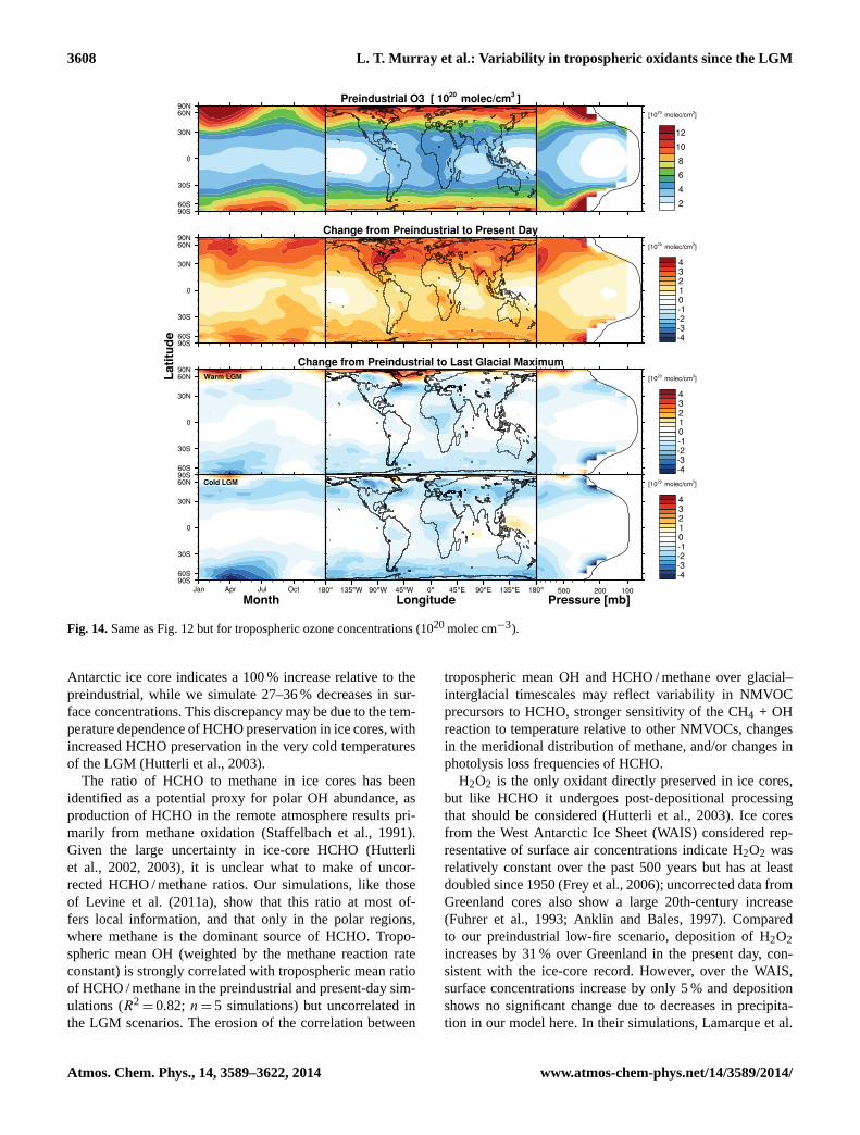
3608 L. T. Murray et al.: Variability in tropospheric oxidants since the LGM
Murray et al.: Variability in tropospheric oxidants since the LGM 39
Month Pressure [mb]Longitude
La
titu
de
]
]
]
]
Fig. 14. Same as Fig. 12, but for tropospheric ozone concentrations (1020 molec cm−3).Fig. 14.Same as Fig.12but for tropospheric ozone concentrations (1020molec cm−3).
Antarctic ice core indicates a 100 % increase relative to thepreindustrial, while we simulate 27–36 % decreases in sur-face concentrations. This discrepancy may be due to the tem-perature dependence of HCHO preservation in ice cores, withincreased HCHO preservation in the very cold temperaturesof the LGM (Hutterli et al., 2003).
The ratio of HCHO to methane in ice cores has beenidentified as a potential proxy for polar OH abundance, asproduction of HCHO in the remote atmosphere results pri-marily from methane oxidation (Staffelbach et al., 1991).Given the large uncertainty in ice-core HCHO (Hutterliet al., 2002, 2003), it is unclear what to make of uncor-rected HCHO / methane ratios. Our simulations, like thoseof Levine et al.(2011a), show that this ratio at most of-fers local information, and that only in the polar regions,where methane is the dominant source of HCHO. Tropo-spheric mean OH (weighted by the methane reaction rateconstant) is strongly correlated with tropospheric mean ratioof HCHO / methane in the preindustrial and present-day sim-ulations (R2
= 0.82; n = 5 simulations) but uncorrelated inthe LGM scenarios. The erosion of the correlation between
tropospheric mean OH and HCHO / methane over glacial–interglacial timescales may reflect variability in NMVOCprecursors to HCHO, stronger sensitivity of the CH4 + OHreaction to temperature relative to other NMVOCs, changesin the meridional distribution of methane, and/or changes inphotolysis loss frequencies of HCHO.
H2O2 is the only oxidant directly preserved in ice cores,but like HCHO it undergoes post-depositional processingthat should be considered (Hutterli et al., 2003). Ice coresfrom the West Antarctic Ice Sheet (WAIS) considered rep-resentative of surface air concentrations indicate H2O2 wasrelatively constant over the past 500 years but has at leastdoubled since 1950 (Frey et al., 2006); uncorrected data fromGreenland cores also show a large 20th-century increase(Fuhrer et al., 1993; Anklin and Bales, 1997). Comparedto our preindustrial low-fire scenario, deposition of H2O2increases by 31 % over Greenland in the present day, con-sistent with the ice-core record. However, over the WAIS,surface concentrations increase by only 5 % and depositionshows no significant change due to decreases in precipita-tion in our model here. In their simulations,Lamarque et al.
Atmos. Chem. Phys., 14, 3589–3622, 2014 www.atmos-chem-phys.net/14/3589/2014/

L. T. Murray et al.: Variability in tropospheric oxidants since the LGM 3609
40 Murray et al.: Variability in tropospheric oxidants since the LGM
]
]
]
]
Month Pressure [mb]Longitude
La
titu
de
Fig. 15. Same as Fig. 12, but for H2O2 (1019 molec cm−3).Fig. 15.Same as Fig.12but for H2O2 (1019molec cm−3).
Table 6.Global sources, sinks, and lifetimes for tropospheric H2O2
Emissions Fixed lightning High fire Low fire
ClimateLGM
Preind.LGM
Preind.LGM
Preind.Present
Cold Warm Cold Warm Cold Warm ModelE GEOS4
Burden (Tmol) 0.03 0.05 0.08 0.06 0.08 0.11 0.04 0.06 0.08 0.10 0.12Sources (Tmol year−1)
Chemical production 10 16 23 16 24 33 10 17 23 32 33Sinks (Tmol year−1)
Chemical loss 6 10 14 9 14 19 6 10 14 19 22Dry deposition 1 1 2 2 2 3 1 2 2 3 4Wet deposition 3 5 8 5 7 11 3 5 8 10 7
Lifetime (h) 30 28 29 33 30 29 33 30 29 28 32
(2011) attribute the late-20th century increase in the WAISrecord to the ozone hole, whose heterogeneous chemistry wedo not simulate here. The preindustrial high-fire simulation isinconsistent with the ice-core data, as it implies lower H2O2surface concentrations and deposition everywhere in thepresent day relative to the preindustrial. For the LGM, uncor-
rected measurements from Law Dome in East Antarctica im-ply decreases in H2O2 relative to the preindustrial (vanOm-men and Morgan, 1996), generally matched by reduced de-position fluxes in our simulations despite enhanced surfaceconcentrations. Surface concentrations over East Antarcticagenerally increase relative to the preindustrial in our various
www.atmos-chem-phys.net/14/3589/2014/ Atmos. Chem. Phys., 14, 3589–3622, 2014

3610 L. T. Murray et al.: Variability in tropospheric oxidants since the LGM
LGM simulations because of enhanced polar OH production(Sect.5.1) and decreased precipitation (Sect.3.2), with largevariability reflecting the wide spread in the LGM fire emis-sions as HOx precursors.
Our present-day simulation matches the mean CO surfaceconcentration of 49 ppbv measured at the South Pole by theNOAA Global Monitoring Division for the 1990s, as well asthe southern hemispheric gradient in CO. Carbon monoxidehas been recorded in ice-core air bubbles over the past twomillennia.Wang et al.(2010) measured ice-core concentra-tions of CO at the South Pole of 47± 4 ppbv for 1770. Ourlow-fire preindustrial scenario yields 35 ppbv surface CO atthe South Pole, consistent withWang et al.(2010), given thatas much as 10 ppbv of CO in Antarctic ice cores may derivefrom in situ production (Haan and Raynaud, 1998). Our high-fire simulations yield much higher surface concentrations of63 ppbv at the preindustrial, a value that is greater than anyover the entire CO ice-core record for Antarctica.
Black carbon deposited in Greenland ice cores increasedfrom 1850 to 1950 due to human industrial activity, but thendeclined to the 1800 values by the late 1950s (McConnellet al., 2007). Records of black carbon deposition to Antarc-tica for 1850–2000 imply mostly constant deposition rates(Bisiaux et al., 2012). Squaring these records of black carbondeposition with our model results is challenging. Our high-fire scenario for the preindustrial implies 40–50 % decreasesin black carbon deposition to both Greenland and Antarcticafrom the 1770s to the present day, not consistent with ob-servations. Our low-fire preindustrial scenario yields a bet-ter match with the observations over Antarctica, with similarrates of deposition in the 1770s and the present day. But thissame scenario indicates large, 40–500 %, increases in blackcarbon deposited to Greenland in the present day relative tothe 1770s. Reconciling both the black carbon and CO ice-core records with current understanding of trends in biomassburning is a direction for future research.
Antarctic ice cores show increased sea salt aerosol deposi-tion during cold periods, perhaps as a result of enhanced seasalt emission from frost flowers across the greater expanseof sea ice (Wolff , 2003; Wolff et al., 2006; Fischer et al.,2007; Rothlisberger et al., 2008; Röthlisberger et al., 2010;Wolff et al., 2010). GEOS-Chem assumes no source of seasalt from sea ice (Fig.6e; Jaeglé et al., 2011), and thereforepredicts 70–90 % decreases in sea salt deposition to Antarc-tica in the LGM climate relative to the preindustrial.
The 117O of ice-core sulfate measures the departurefrom mass-dependent fractionation in its oxygen isotopes(Thiemens, 2006). It provides a constraint for assessing therelative importance of different sulfate chemical productionpathways, i.e., gas-phase oxidation by OH vs. aqueous-phaseproduction via H2O2 or ozone, as the latter imparts a large117O signature (Savarino et al., 2000). Measurements fromthe Vostok ice core in Antarctica imply that gas-phase oxida-tion by OH contributed up to 40 % more to sulfate production
during the LGM relative to the interglacial periods that camebefore or after (Alexander et al., 2002).
Our results appear consistent with these measurements of117O of sulfate. In our LGM scenarios, surface concentra-tions of OH at the poles increase, driven primarily by thereduction in methane, CO, and overhead ozone, as well as in-creases in surface UV albedo. In addition, the fraction of SO2oxidized in the gas phase by OH increases throughout theLGM troposphere, reflecting a global decrease in aqueous-phase chemistry in the drier climate.
Unlike sulfate, nitrate aerosol undergoes substantial post-depositional photochemical processing via evaporation ofHNO3 (Rothlisberger et al., 2002) and photolysis to produceNOx (Honrath et al., 1999, 2000). Photolysis of snow ni-trate to produce NOx is thought to be dominant (Davis et al.,2008; Erbland et al., 2012). The degree of post-depositionalprocessing depends mainly on snow accumulation rate. InEast Antarctica, where the snow accumulation rate is low,it is thought that all of the nitrate originally deposited to thesnow is photolyzed to NOx during austral spring and summer(Erbland et al., 2012). This NOx is released to the boundarylayer, where it is re-oxidized locally and redeposited to thesnow surface as nitrate. The117O signature in East Antarc-tic ice-core nitrate thus reflects the relative abundance of lo-cal atmospheric oxidants ozone and RO2. At locations withhigher snow accumulation rates such as Greenland and WestAntarctica, the117O of nitrate may reflect a combination ofthe local summertime ozone / RO2 ratio and that ratio in theNOx source regions.
For the present day, our low-fire simulations yield a 4 %increase in the ozone / RO2 ratio over Greenland and a 7 %decrease over the WAIS, qualitatively consistent with the ex-pected sign changes from ice-core measurements of117O ofnitrate (Alexander et al., 2004; Sofen et al., 2014). For theLGM, we calculate 20–40 % increases in the ozone / RO2 ra-tio over East Antarctica relative to the preindustrial, and upto a 50 % increase over Greenland. Over Greenland, the in-creases result from increases in both tropospheric ozone fromlocal enhanced stratospheric downwelling (Fig.14) and re-ductions in RO2. Over Antarctica, ozone decreases in bothLGM scenarios, so decreases in RO2 largely dominate theresponse. Observations of nitrate117O in the LGM are notyet published, but are currently being collected.
7 Implications for the methane budget
Table7 gives the global methane lifetime against OH oxida-tion in the troposphere (τCH4,OH) for each simulation, whichlargely determines the removal efficiency of methane fromthe atmosphere. We findτCH4,OH in our present-day simula-tions decreases by 7± 3 % relative to the preindustrial. In thewarm-LGM scenario,τCH4,OH changes little from the prein-dustrial (0.2± 6 %), but increases by 35± 16 % in the cold-LGM scenario. In our most likely representation of change
Atmos. Chem. Phys., 14, 3589–3622, 2014 www.atmos-chem-phys.net/14/3589/2014/

L. T. Murray et al.: Variability in tropospheric oxidants since the LGM 3611
across the glacial–interglacial period, with low fire and warmLGM, τCH4,OH is 4.5 % higher at the LGM than in the prein-dustrial. We diagnose these changes below.
The value ofτCH4,OH is given by the global burden (Tg)divided by the total loss rate in the troposphere (Tg year−1),i.e.,
τCH4,OH =
TOA∫surface
[CH4]dx dy dp
tropopause∫surface
kCH4+OH(T )[OH][CH4]dx dy dp
. (2)
It therefore responds to convolved changes in the tropo-spheric OH and methane distributions and the strong tem-perature kinetic effect (2.4 % K−1 at 273 K) on the reactionrate constant,kCH4+OH (Lawrence et al., 2001; Sander et al.,2011; John et al., 2012). The temperature changes alonecauseτCH4,OH to increase by 4.2 % in the warm-LGM sce-nario and 20 % in the cold-LGM relative to the preindustrial,and decrease by 1.4 % at the present day. At the LGM, thiseffect is partially countered by the shift of the methane max-imum from the northern high latitudes to the tropics, whichby itself leads to a 1.9 % decrease inτCH4,OH. Changes inthe methane meridional distribution are negligible from thepreindustrial to present, despite the large change in the meanconcentration. The kinetic temperature and methane distri-bution effects are then offset or enhanced by changes in OHresponding to the factors outlined in Sect.5.1. In the presentday, the kinetic effect is augmented by the increase in tropo-spheric mean OH, and the lifetime decreases relative to thepreindustrial. In the warm-LGM scenario, the net effect ofthe changes in temperature and methane distribution is small,and therefore changes in OH dominateτCH4,OH. In the cold-LGM scenario, the temperature kinetic effect guarantees thatτCH4,OH increases relative to the preindustrial.
That τCH4,OH remains nearly constant or increases at theLGM in our simulations puts a higher burden on sources inexplaining the glacial–interglacial variability of atmosphericmethane concentrations recorded in ice cores. In their modelstudy, which did not include a paleo-stratosphere,Levineet al. (2011c) concluded that the effects of temperature andbiogenic VOCs cancel each other out such that observedchanges in ice-core methane must be driven primarily bysources. Our findings confirm those ofLevine et al.(2011c),and extend them to include changes in overhead ozone andNOx, which together may even drive decreased OH at theLGM relative to the preindustrial.
Assuming no large changes occurred in the minor lossmechanisms for methane (soils and stratospheric OH;IPCC,2007), the source of methane emissions scales as its loss byOH in the troposphere (Table7 and Fig.9). We estimate thatthe methane loss frequency in the stratosphere changes lessthan 1 % since the LGM in our simulations; the effect of re-duced stratospheric water vapor at the LGM is largely offsetby temperature increases. Our results imply that relative to
the preindustrial, total methane emissions are 150 % higherin the present, and are reduced by 42–65 % at the LGM, witha 50 % reduction our best estimate. These estimated reduc-tions at the LGM are greater than the 29–42 % decrease inwetland emissions simulated by the PMIP2 ensemble mem-bers (Weber et al., 2010), and much larger than the 16 and23 % decreases in natural methane emissions simulated byKaplan et al.(2006) andValdes et al.(2005) over the sameperiod. However, we note that if the tropical fraction of to-tal methane in LGM were to increase by 33 % as implied bya Bolivian ice core (Campen, 2000) – an extremely unlikelyscenario (Sect.2.4) – the implied methane source would infact be consistent with the previous bottom-up estimates, asthe integrated loss rate of methane (denominator of Eq.2)would increase despite the reductions in OH and tempera-ture.
8 Discussion and conclusions
We present a stepwise, offline-coupled modeling frameworkfor simulating paleo-oxidant levels since the LGM. Our goalis to test within a 3-D model framework the sensitivity oftropospheric oxidants over a range of likely forcings fromclimate-driven and anthropogenic changes. Archived mete-orology from the GISS ModelE GCM is used to drive theBIOME4-TG global equilibrium terrestrial vegetation modeland the LPJ-LMfire fire model. We also apply the Mod-elE meteorology to the GEOS-Chem CTM, together withthe BIOME4-TG vegetation structure and LPJ-LMfire emis-sions. We then perform detailed simulations of troposphericcomposition with an online-coupled linearized stratosphericchemistry scheme. Offline coupling allows for rapid sensi-tivity tests and identification of first-order effects of chang-ing climate on composition. However, it does not enable theexamination of chemical feedbacks on climate, which wouldrequire a fully integrated Earth system model, such as Mod-elE2 (Shindell et al., 2013).
We simulate four different time slices with the GCM: thepresent day (ca. 1990s); preindustrial (ca. 1770s); and twopossible realizations of the Last Glacial Maximum (LGM;21 ka), one significantly colder than the other, reflecting un-certainty in the extent of tropical cooling at the LGM. Theclimate simulations are forced by prescribing greenhouse gaslevels, orbital parameters, SSTs, sea ice extent, and ice sheettopography. Reductions in greenhouse gases drive decreasesin tropospheric temperatures and water vapor, and deceleratethe stratospheric residual circulation, consistent with earlierwork (Braconnot et al., 2007a; Bartlein et al., 2011; Rindet al., 2009). Relative to preindustrial, tropical surface airtemperatures are 1.4◦C colder in the warm-LGM scenarioand 6.8◦C colder in the cold-LGM scenario; the preindustrialto present-day change is+0.5◦C. Reduced stratospheric cir-culation leads to an increase in tropical stratospheric ozonecolumns, which strongly affect tropospheric photolysis rates.
www.atmos-chem-phys.net/14/3589/2014/ Atmos. Chem. Phys., 14, 3589–3622, 2014

3612 L. T. Murray et al.: Variability in tropospheric oxidants since the LGM
Table 7.Global methane burden and lifetime against tropospheric oxidation by OH (τCH4,OH).
Emission Scenario Fixed lightning High fire Low fire Present day
Climate Cold Warm Preind. Cold Warm Preind. Cold Warm Preind. ModelE GEOS4 LiteratureLGM LGM LGM LGM LGM LGM
CH4 burden [Tg]a 1040 1040 2000 1040 1040 2000 1040 1040 2000 4780 4780 4850b
Loss by OH in troposphere [Tg year−1] 82 100 184 64 90 174 66 90 181 460 481 512c
OH, kCH4+OH-weighted [105 molec cm−3]d 12.9 13.6 12.3 10.1 12.2 11.6 11.0 13.0 12.1 12.7 13.0τCH4,OH [year] 12.8 10.4 10.9 16.4 11.6 11.5 15.9 11.6 11.1 10.4 9.9 10.2+0.9
−0.7e
a Global burden calculated from mean surface concentration using a conversion factor of 2.75 TgCH4 ppbv−1 (Prather et al., 2012). b IPCC(2001). c IPCC(2007).d Tropospheric mean OH, weighted bykCH4+OH(T )MCH4
, wherekCH4+OH(T ) is the temperature-dependent rate coefficient for reaction of CH4 with OH, andMCH4is the mass of CH4 in the grid box.
e Prinn et al.(2005), inferred from methyl chloroform observations.
Tropospheric trace gas and aerosol emissions respond toclimate, and we simulate reductions in most trace gas emis-sions in cooler climates. Terrestrial plant VOC emissions areinfluenced by both land cover and meteorology. A decreasein the present day relative to the preindustrial results fromexpansions in cropland. In the LGM, the cooler temperaturesultimately drive decreases in plant VOC emissions relative tothe preindustrial. Soil microbial emissions of NOx also de-crease with reduced temperatures and precipitation fluxes atthe LGM. Lightning responds to the vertical extent of deepconvection, and therefore decreases at the LGM, especiallyin the cold-LGM scenario. We also test a scenario in whichwe fix total lightning emissions. Estimates of biomass burn-ing emissions in past atmospheres are highly uncertain; wetest the extremes in the range of estimates at the LGM (10and 200 % of present) and the preindustrial (100 and 320 %of present) using distributions of dry matter burned from theLPJ-LMfire model.
We find net reductions in all oxidants in past atmospheresrelative to the present day, except for H2O2 in the high-fire preindustrial simulation, and OH in the fixed lightningLGM scenarios. OH is relatively well buffered in compar-ison with the other oxidants. It is relatively insensitive tochanges in anthropogenic and fire emissions, but sensitiveto lightning. In our simulations, OH increases at the presentday by+7.0± 4.3 %, and shows little change at the LGM(0.5 ± 12 %), both relative to the preindustrial. A linear re-lationship with JO3qSN/(S
3/2C ) explains 72 % of the total
variability seen in the mean OH burdens of our 11 simula-tions.JO3 andq largely regulate primary production of HOx,
whereasSN/(S3/2C ) largely influences HOx partitioning be-
tween OH and RO2 (but also primary production).Most previous studies lacked realistic paleo-stratospheres
and simulated larger increases in OH at the LGM (cf. Ta-ble 1). Our work suggests that OH changes were more tem-pered, and possibly even reduced at the LGM. Of the vari-ous emission sources, lightning is most capable of perturb-ing SN/(S
3/2C ), as it makes up a relatively large fraction of
SN (37±16 % ofSN in past atmospheres; 14 % in the presentday), andSN � SC. Unlike anthropogenic or fire emissions,NOx from lightning also lacks any co-emissions of reactivecarbon, and it is relatively uncorrelated with a competing
emission source, as soil NOx emissions are with those ofbiogenic VOCs. Therefore, we conclude that the three fac-tors OH is most sensitive to on glacial–interglacial timescalesare overhead ozone, tropospheric water vapor, and lightningemissions. These factors should be given particular attentionin future studies.
Ozone in our simulations increases by 24± 11 % at thepresent and decreases by 12± 10 % at the LGM, relativeto the preindustrial. Our changes are consistent with priorstudies but more tempered, likely reflecting the high bias inthe source of ozone transported from the stratosphere. Thatsource decreases in magnitude in the colder climates follow-ing the deceleration of the stratospheric circulation, but nev-ertheless becomes an increasingly large fraction of the totalsource. We extend to LGM conditions the finding that globalmean ozone from 1850 through 2100 depends strongly onSN (Stevenson et al., 2006; Young et al., 2013). Ozone pro-duction efficiencies per unit NOx emitted increase in eachsuccessively colder atmosphere.
H2O2 responds to changes in both climate and emissions,varying more strongly in its production pathways across thedifferent scenarios than in its loss rates via wet deposition.We find that H2O2 abundance is very sensitive to fire emis-sions, as these emissions generate HOx. Ice-core H2O2 maytherefore act as a useful proxy for paleo fire emissions as wellas for biogenic emissions, another HOx source. Nitrate radi-cal is directly related to the total source of reactive nitrogen,SN (R2=0.97).
Our simulations are broadly qualitatively consistent withice-core records of117O in sulfate and nitrate at the LGM,and CO, HCHO, black carbon, and H2O2 in the preindustrial.Comparison with black carbon, CO and H2O2 preserved inice cores indicate that fire emissions during the preindustrialand LGM likely fall closer to the lower end of the estimatedrange. Our simulations indicate that the HCHO / methane ra-tio cannot serve as a proxy for global OH variability, evenfrom future tropical ice cores.
Finally, our work provides greater certainty in the break-down of the atmospheric methane budget at the LGM. Priorstudies disagree as to the relative role of sources vs. sinksin explaining the large glacial–interglacial variability in at-mospheric methane concentrations recorded in ice cores. We
Atmos. Chem. Phys., 14, 3589–3622, 2014 www.atmos-chem-phys.net/14/3589/2014/
L. T. Murray et al.: Variability in tropospheric oxidants since the LGM 3613
simulate nearly constant or increased methane lifetimes atthe LGM relative to the preindustrial, implying that the largeglacial–interglacial variability seen in ice-core methane ispredominantly driven by changing methane sources. Our re-sults imply that methane emissions decreased by 50 % at theLGM relative to the preindustrial, a greater change than re-ported in previous bottom-up estimates.
Supplementary material related to this article isavailable online athttp://www.atmos-chem-phys.net/14/3589/2014/acp-14-3589-2014-supplement.pdf.
Acknowledgements.The authors would like to thank C. McLinden(Environment Canada) for providing updated Linoz coefficientsfor the past atmospheres, N. Mahowald (Cornell U.) for providingLGM mineral dust burdens, A. LeGrande (NASA GISS) forproviding LGM boundary conditions for the GCM, and G. Schmidt(NASA GISS) and P. Lin (UW/NOAA GFDL) for useful discus-sions. This project was funded by NSF grant AGS-1102880 toHarvard University and the University of Washington.
Edited by: P. Jöckel
References
Adams, J. M., Constable, J. V. H., Guenther, A. B., and Zimmerman,P.: An estimate of natural volatile organic compound emissionsfrom vegetation since the last glacial maximum, Atmos. Envi-ron., 3, 73–91, 2001.
Alexander, B., Savarino, J., Barkov, N., Delmas, R., andThiemens, M. H.: Climate driven changes in the oxidation path-ways of atmospheric sulfur, Geophys. Res. Lett., 29, 1685,doi:10.1029/2002GL014879, 2002.
Alexander, B., Savarino, J., Kreutz, K., and Thiemens, M. H.: Im-pact of preindustrial biomass-burning emissions on the oxidationpathways of tropospheric sulfur and nitrogen, J. Geophys. Res.-Atmos., 109, D08303, doi:10.1029/2003JD004218, 2004.
Allen, D. J., Pickering, K., Duncan, B., and Damon, M.: Im-pact of lightning NO emissions on North American photo-chemistry as determined using the Global Modeling Initia-tive (GMI) model, J. Geophys. Res.-Atmos., 115, D22301,doi:10.1029/2010JD014062, 2010.
Anklin, M. and Bales, R. C.: Recent increase in H2O2 concentrationat Summit, Greenland, J. Geophys. Res.-Atmos., 102, 19099–19104, 1997.
Auvray, M. and Bey, I.: Long-range transport to Europe:Seasonal variations and implications for the Europeanozone budget, J. Geophys. Res.-Atmos., 110, D11303,doi:10.1029/2004JD005503, 2005.
Balkanski, Y., Jacob, D. J., Gardner, G., Graustein, W., andTurekian, K.: Transport and Residence Times of TroposphericAerosols Inferred From a Global 3-Dimensional Simulation ofPb-210, J. Geophys. Res.-Atmos., 98, 20573–20586, 1993.
Bartlein, P. J., Harrison, S. P., Brewer, S., Connor, S., Davis, B.A. S., Gajewski, K., Guiot, J., Harrison-Prentice, T. I., Hender-son, A., Peyron, O., Prentice, I. C., Scholze, M., Seppa, H., Shu-man, B., Sugita, S., Thompson, R. S., Viau, A. E., Williams, J.,and Wu, H.: Pollen-based continental climate reconstructions at 6and 21 ka: a global synthesis, Clim. Dynam., 37, 775–802, 2011.
Berger, A. L.: Long-term variations of daily insolation and Quater-nary climatic changes, J. Atmos. Sci., 35, 2362–2367, 1978.
Berntsen, T. K., Isaksen, I. S. A., Myhre, G., Fuglestvedt, J. S.,Stordal, F., Larsen, T. A., Freckleton, R. S., and Shine, K. P.:Effects of anthropogenic emissions on tropospheric ozone andits radiative forcing, J. Geophys. Res., 102, 28101–28126,doi:10.1029/97JD02226, 1997.
Bey, I., Jacob, D. J., Yantosca, R., Logan, J. A., Field, B., Fiore, A.,Li, Q., Liu, H., Mickley, L., and Schultz, M.: Global modeling oftropospheric chemistry with assimilated meteorology: Model de-scription and evaluation, J. Geophys. Res.-Atmos., 106, 23073–23095, 2001.
Bisiaux, M. M., Edwards, R., McConnell, J. R., Curran, M. A.J., Van Ommen, T. D., Smith, A. M., Neumann, T. A., Pas-teris, D. R., Penner, J. E., and Taylor, K.: Changes in black car-bon deposition to Antarctica from two high-resolution ice corerecords, 1850–2000 AD, Atmos. Chem. Phys., 12, 4107–4115,doi:10.5194/acp-12-4107-2012, 2012.
Blunier, T., Chappellaz, J., Schwander, J., Dällenbach, A., Stauf-fer, B., Stocker, T. F., Raynaud, D., Jouzel, J., Clausen, H. B.,Hammer, C. U., and Johnsen, S. J.: Asynchrony of Antarctic andGreenland climate change during the last glacial period, Nature,394, 739–743, 1998.
Bock, J., Martinerie, P., Witrant, E., and Chappellaz, J.: Atmo-spheric impacts and ice core imprints of a methane pulse fromclathrates, Earth Planet. Sc. Lett., 349–350, 98–108, 2012.
Bousquet, P., Ringeval, B., Pison, I., Dlugokencky, E. J., Brunke, E.-G., Carouge, C., Chevallier, F., Fortems-Cheiney, A., Franken-berg, C., Hauglustaine, D. A., Krummel, P. B., Langenfelds, R.L., Ramonet, M., Schmidt, M., Steele, L. P., Szopa, S., Yver,C., Viovy, N., and Ciais, P.: Source attribution of the changes inatmospheric methane for 2006–2008, Atmos. Chem. Phys., 11,3689–3700, doi:10.5194/acp-11-3689-2011, 2011.
Braconnot, P., Otto-Bliesner, B., Harrison, S., Joussaume, S., Pe-terchmitt, J.-Y., Abe-Ouchi, A., Crucifix, M., Driesschaert, E.,Fichefet, Th., Hewitt, C. D., Kageyama, M., Kitoh, A., Laîné,A., Loutre, M.-F., Marti, O., Merkel, U., Ramstein, G., Valdes,P., Weber, S. L., Yu, Y., and Zhao, Y.: Results of PMIP2 coupledsimulations of the Mid-Holocene and Last Glacial Maximum –Part 1: experiments and large-scale features, Clim. Past, 3, 261–277, doi:10.5194/cp-3-261-2007, 2007a.
Braconnot, P., Otto-Bliesner, B., Harrison, S., Joussaume, S., Pe-terchmitt, J.-Y., Abe-Ouchi, A., Crucifix, M., Driesschaert, E.,Fichefet, Th., Hewitt, C. D., Kageyama, M., Kitoh, A., Loutre,M.-F., Marti, O., Merkel, U., Ramstein, G., Valdes, P., Weber,L., Yu, Y., and Zhao, Y.: Results of PMIP2 coupled simula-tions of the Mid-Holocene and Last Glacial Maximum – Part2: feedbacks with emphasis on the location of the ITCZ andmid- and high latitudes heat budget, Clim. Past, 3, 279–296,doi:10.5194/cp-3-279-2007, 2007b.
Braconnot, P., Harrison, S. P., Kageyama, M., Bartlein, P. J.,Masson-Delmotte, V., Abe-Ouchi, A., Otto-Bliesner, B., and
www.atmos-chem-phys.net/14/3589/2014/ Atmos. Chem. Phys., 14, 3589–3622, 2014

3614 L. T. Murray et al.: Variability in tropospheric oxidants since the LGM
Zhao, Y.: Evaluation of climate models using palaeoclimaticdata, Nature Clim. Change, 2, 417–424, 2012.
Brasseur, G., Kiehl, J., Muller, J., Schneider, T., Granier, C., Tie, X.,and Hauglustaine, D.: Past and future changes in global tropo-spheric ozone: Impact on radiative forcing, Geophys. Res. Lett.,25, 3807–3810, 1998.
Brook, E. J., Harder, S., Severinghaus, J., Steig, E. J., and Sucher,C. M.: On the origin and timing of rapid changes in atmosphericmethane during the Last Glacial Period, Global Biogeochem.Cy., 14, 559–572, 2000.
Campen, R. K.: Measurements of gasses trapped in a South Ameri-can ice core: Paleoatmospheric composition and inferred micro-bial activity, Master’s thesis, Pennsylvania State University, 146pp., 2000.
Campen, R. K., Sowers, T., and Alley, R. B.: Evidence of microbialconsortia metabolizing within a low-latitude mountain glacier,Geology, 31, 231–234, 2003.
Castebrunet, H., Genthon, C., and Martinerie, P.: Sulfurcycle at Last Glacial Maximum: Model results versusAntarctic ice core data, Geophys. Res. Lett., 33, L22711,doi:10.1029/2006GL027681, 2006.
Chappellaz, J., Barnola, J. M., Raynaud, D., Korotkevich, Y. S., andLorius, C.: Ice-core record of atmospheric methane over the past160,000 years, Nature, 345, 127–131, 1990.
Chappellaz, J., Blunier, T., Raynaud, D., Barnola, J. M., Schwander,J., and Stauffert, B.: Synchronous changes in atmospheric CH4and Greenland climate between 40 and 8 kyr BP, Nature, 366,443–445, 1993.
Chappellaz, J., Blunier, T., Kints, S., Dällenbach, A., Barnola, J.-M., Schwander, J., Raynaud, D., and Stauffer, B.: Changes inthe atmospheric CH4 gradient between Greenland and Antarc-tica during the Holocene, J. Geophys. Res., 102, 15987–15997,doi:10.1029/97JD01017, 1997.
Chen, Y. H. and Prinn, R. G.: Estimation of atmospheric methaneemissions between 1996 and 2001 using a three-dimensionalglobal chemical transport model, J. Geophys. Res.-Atmos., 111,D10307, doi:10.1029/2005JD006058, 2006.
Chin, M., Rood, R. B., Lin, S. J., Muller, J.-F., and Thompson,A. M.: Atmospheric sulfur cycle simulated in the global modelGOCART- Model description and global properties, J. Geophys.Res., 105, 24671–24687, 2000.
Christian, H., Blakeslee, R., Boccippio, D., Boeck, W., Buechler,D., Driscoll, K., Goodman, S., Hall, J., Koshak, W., Mach, D.,and Stewart, M.: Global frequency and distribution of lightningas observed from space by the Optical Transient Detector, J.Geophys. Res.-Atmos., 108, 4005, doi:10.1029/2002JD002347,2003.
Clark, P. U. and Mix, A. C.: Ice sheets and sea level of the LastGlacial Maximum, Quaternary Sci. Rev., 21, 1–7, 2002.
CLIMAP: Surface of Ice-Age Earth, Science, 191, 1131–1137,1976.
Collins, W. J., Sitch, S., and Boucher, O.: How vegetation impactsaffect climate metrics for ozone precursors, J. Geophys. Res.,115, D23308, doi:10.1029/2010JD014187, 2010.
Considine, D. B., Logan, J. A., and Olsen, M. A.: Evalu-ation of near-tropopause ozone distributions in the GlobalModeling Initiative combined stratosphere/troposphere modelwith ozonesonde data, Atmos. Chem. Phys., 8, 2365–2385,doi:10.5194/acp-8-2365-2008, 2008.
Crutzen, P. J. and Brühl, C.: A model study of atmospheric tem-peratures and the concentrations of ozone, hydroxyl, and someother photochemically active gases during the glacial, the pre-industrial Holocene and the present, Geophys. Res. Lett., 20,1047–1050, 1993.
Crutzen, P. J. and Zimmermann, P. H.: The changing photochem-istry of the troposphere, Tellus B, 43, 136–151, 1991.
Davis, D., Seelig, J., Huey, G., Crawford, J., Chen, G., Wang, Y.,Buhr, M., Helmig, D., Neff, W., and Blake, D.: A reassessmentof Antarctic plateau reactive nitrogen based on ANTCI 2003airborne and ground based measurements, Atmos. Environ., 42,2831–2848, 2008.
Delaygue, G., Masson, V., Jouzel, J., Koster, R. D., and Healy, R. J.:The origin of Antarctic precipitation: a modelling approach, Tel-lus B, 52, 19–36, 2000.
Diehl, T.: A Global Inventory of Volcanic SO2 Emissionsfor Hindcast Scenarios,http://www-lscedods.cea.fr/aerocom/AEROCOM_HC/volc, 2009.
Dlugokencky, E. J., Lang, P. M., Crotwell, A. M., Masarie,K. A., and Crotwell, M. J.: Atmospheric Methane Dry AirMole Fractions from the NOAA ESRL Carbon Cycle Cooper-ative Global Air Sampling Network, 1983–2007, Version: 2008-07-02, Path:ftp://aftp.cmdl.noaa.gov/data/trace_gases/ch4/flask/surface/, 2008.
Duncan, B. N., Logan, J. A., Bey, I., Megretskaia, I. A., Yan-tosca, R. M., Novelli, P. C., Jones, N. B., and Rinsland, C. P.:Global budget of CO, 1988–1997: Source estimates and valida-tion with a global model, J. Geophys. Res.-Atmos., 112, D22301,doi:10.1029/2007JD008459, 2007.
Engel, A., Möbius, T., Bönisch, H., Schmidt, U., Heinz, R., Levin,I., Atlas, E., Aoki, S., Nakazawa, T., Sugawara, S., Moore, F.,Hurst, D., Elkins, J., Schauffler, S., Andrews, A., and Boering,K.: Age of stratospheric air unchanged within uncertainties overthe past 30 years, Nature, 2, 28–31, 2008.
Erbland, J., Vicars, W. C., Savarino, J., Morin, S., Frey, M. M.,Frosini, D., Vince, E., and Martins, J. M. F.: Air–snow transferof nitrate on the East Antarctic Plateau – Part 1: Isotopic evi-dence for a photolytically driven dynamic equilibrium in sum-mer, Atmos. Chem. Phys., 13, 6403–6419, doi:10.5194/acp-13-6403-2013, 2013.
Etheridge, D. M., Steele, L. P., Francey, R. J., and Langenfelds,R. L.: Atmospheric methane between 1000 A.D. and present:Evidence of anthropogenic emissions and climatic variability,J. Geophys. Res., 103, 15979–15993, doi:10.1029/98JD00923,1998.
Fernandes, S. D., Trautmann, N. M., Streets, D. G., Roden, C. A.,and Bond, T. C.: Global biofuel use, 1850–2000, Global Bio-geochem. Cy., 21, GB2019, doi:10.1029/2006GB002836, 2007.
Fiore, A. M., Dentener, F. J., Wild, O., Cuvelier, C., Schultz, M. G.,Hess, P., Textor, C., Schulz, M., Doherty, R. M., Horowitz, L. W.,MacKenzie, I. A., Sanderson, M. G., Shindell, D. T., Steven-son, D. S., Szopa, S., Van Dingenen, R., Zeng, G., Atherton,C., Bergmann, D., Bey, I., Carmichael, G., Collins, W. J., Dun-can, B. N., Faluvegi, G., Folberth, G., Gauss, M., Gong, S.,Hauglustaine, D., Holloway, T., Isaksen, I. S. A., Jacob, D. J.,Jonson, J. E., Kaminski, J. W., Keating, T. J., Lupu, A., Marmer,E., Montanaro, V., Park, R. J., Pitari, G., Pringle, K. J., Pyle,J. A., Schroeder, S., Vivanco, M. G., Wind, P., Wojcik, G.,Wu, S., and Zuber, A.: Multimodel estimates of intercontinental
Atmos. Chem. Phys., 14, 3589–3622, 2014 www.atmos-chem-phys.net/14/3589/2014/

L. T. Murray et al.: Variability in tropospheric oxidants since the LGM 3615
source-receptor relationships for ozone pollution, J. Geophys.Res.-Atmos., 114, D04301, doi:10.1029/2008JD010816, 2009.
Fiore, A. M., Naik, V., Spracklen, D. V., Steiner, A., Unger, N.,Prather, M., Bergmann, D., Cameron-Smith, P. J., Cionni, I.,Collins, W. J., Dalsoren, S., Eyring, V., Folberth, G. A., Ginoux,P., Horowitz, L. W., Josse, B., Lamarque, J.-F., MacKenzie, I. A.,Nagashima, T., O’Connor, F. M., Righi, M., Rumbold, S. T.,Shindell, D. T., Skeie, R. B., Sudo, K., Szopa, S., Takemura, T.,and Zeng, G.: Global air quality and climate, Chem. Soc. Rev.,41, 6663–6683, doi:10.1039/c2cs35095e, 2012.
Fischer, E. V., Jacob, D. J., Millet, D. B., Yantosca, R. M.,and Mao, J.: The role of the ocean in the global atmo-spheric budget of acetone, Geophys. Res. Lett., 39, L01807,doi:10.1029/2011GL050086, 2012.
Fischer, H., Fundel, F., Ruth, U., Twarloh, B., Wegner, A., Udisti,R., Becagli, S., Castellano, E., Morganti, A., Severi, M., Wolff,E., Littot, G. C., Rothlisberger, R., Mulvaney, R., Hutterli, M. A.,Kaufmann, P., Federer, U., Lambert, F., Bigler, M., Hansson, M.,Jonsell, U., De Angelis, M., Boutron, C. F., Siggaard-Andersen,M. L., Steffensen, J. P., Barbante, C., Gaspari, V., Gabrielli, P.,and Wagenbach, D.: Reconstruction of millennial changes in dustemission, transport and regional sea ice coverage using the deepEPICA ice cores from the Atlantic and Indian Ocean sector ofAntarctica, Earth Planet. Sc. Lett., 260, 340–354, 2007.
Fischer, H., Behrens, M., Bock, M., Richter, U., Schmitt, J., Louler-gue, L., Chappellaz, J., Spahni, R., Blunier, T., Leuenberger, M.,and Stocker, T. F.: Changing boreal methane sources and con-stant biomass burning during the last termination, Nature, 452,864–867, 2008.
Fisher, J. A., Jacob, D. J., Wang, Q., Bahreini, R., Carouge,C. C., Cubison, M. J., Dibb, J. E., Diehl, T., Jimenez, J. L.,Leibensperger, E. M., Lu, Z., Meinders, M. B. J., Pye, H. O. T.,Quinn, P. K., Sharma, S., Streets, D. G., van Donkelaar, A., andYantosca, R. M.: Sources, distribution, and acidity of sulfate–ammonium aerosol in the Arctic in winter–spring, Atmos. Envi-ron., 45, 7301–7318, 2011.
Fluckiger, J., Monnin, E., Stauffer, B., Schwander, J., Stocker,T., Chappellaz, J., Raynaud, D., and Barnola, J.: High-resolution Holocene N2O ice core record and its relation-ship with CH4 and CO2, Global Biogeochem. Cy., 16, 1010,doi:10.29/2001GB001417, 2002.
Fountoukis, C. and Nenes, A.: ISORROPIA II: a computationallyefficient thermodynamic equilibrium model for K+-Ca+2 -Mg+
2 -
NH+
4 -Na+-SO2−
4 -NO3–Cl–H2O aerosols, Atmos. Chem. Phys.,7, 4639–4659, doi:10.5194/acp-7-4639-2007, 2007.
Frey, M. M., Bales, R. C., and McConnell, J. R.: Climate sensitiv-ity of the century-scale hydrogen peroxide (H2O2) record pre-served in 23 ice cores from West Antarctica, J. Geophys. Res.,111, D21301, doi:10.1029/2005JD006816, 2006.
Fuhrer, K., Neftel, A., Anklin, M., and Maggi, V.: Continuous mea-surements of hydrogen peroxide, formaldehyde, calcium and am-monium concentrations along the new grip ice core from summit,Central Greenland, Atmos. Environ., 27, 1873–1880, 1993.
Garcia, R. R. and Randel, W. J.: Acceleration of the Brewer-Dobsoncirculation due to increases in greenhouse gases, J. Atmos. Sci.,65, 2731–2739, 2008.
Gillett, R. W., Van Ommen, T. D., Jackson, A. V., and Ayers,G. P.: Formaldehyde and peroxide concentrations in Law Dome(Antarctica) firn and ice cores, J. Glaciol., 46, 15–19, 2000.
Grenfell, J. L., Shindell, D. T., Koch, D., and Rind, D.: Chemistry-climate interactions in the Goddard Institute for Space Studiesgeneral circulation model: 2. New insights into modeling thepreindustrial atmosphere, J. Geophys. Res., 106, 33435–33451,doi:10.1029/2000JD000090, 2001.
Guelle, W., Balkanski, Y., Dibb, J., Schulz, M., and Dulac, F.: Wetdeposition in a global size-dependent aerosol transport model 2.Influence of the scavenging scheme on Pb-210 vertical profiles,surface concentrations, and deposition, J. Geophys. Res.-Atmos.,103, 28875–28891, 1998a.
Guelle, W., Balkanski, Y., Schulz, M., Dulac, F., and Monfray,P.: Wet deposition in a global size-dependent aerosol transportmodel – 1. Comparison of a 1 year Pb-210 simulation withground measurements, J. Geophys. Res.-Atmos., 103, 11429–11445, 1998b.
Guenther, A., Hewitt, C. N., Erickson, D., Fall, R., Geron, C.,Graedel, T., Harley, P., Klinger, L., Lerdau, M., Mckay, W. A.,Pierce, T., Scholes, B., Steinbrecher, R., Tallamraju, R., Tay-lor, J., and Zimmerman, P.: A global model of natural volatileorganic compound emissions, J. Geophys. Res., 100, 8873,doi:10.1029/94JD02950, 1995.
Guenther, A., Baugh, W. M., Brasseur, G. P., Greenberg, J., Harley,P., Klinger, L. F., Serça, D., and Vierling, L. A.: Isoprene emis-sion estimates and uncertainties for the Central African EX-PRESSO study domain, J. Geophys. Res.-Atmos., 104, 30625–30639, 1999.
Guenther, A., Geron, C., Pierce, T., Lamb, B., Harley, P., andFall, R.: Natural emissions of non-methane volatile organic com-pounds; carbon monoxide, and oxides of nitrogen from NorthAmerica, Atmos. Environ., 34, 2205–2230, 2000.
Guenther, A., Karl, T., Harley, P., Wiedinmyer, C., Palmer, P. I.,and Geron, C.: Estimates of global terrestrial isoprene emissionsusing MEGAN (Model of Emissions of Gases and Aerosols fromNature), Atmos. Chem. Phys., 6, 3181–3210, doi:10.5194/acp-6-3181-2006, 2006.
Guenther, A. B., Jiang, X., Heald, C. L., Sakulyanontvittaya, T.,Duhl, T., Emmons, L. K., and Wang, X.: The Model of Emissionsof Gases and Aerosols from Nature version 2.1 (MEGAN2.1): anextended and updated framework for modeling biogenic emis-sions, Geosci. Model Dev., 5, 1471–1492, doi:10.5194/gmd-5-1471-2012, 2012.
Haan, D. and Raynaud, D.: Ice core record of CO variations duringthe last two millennia: atmospheric implications and chemical in-teractions within the Greenland ice, Tellus B, 50, 253–262, 1998.
Haan, D., Martinerie, P., and Raynaud, D.: Ice core data of atmo-spheric carbon monoxide over Antarctica and Greenland duringthe last 200 years, Geophys. Res. Lett., 23, 2235–2238, 1996.
Hansen, J., Sato, M., Ruedy, R., Kharecha, P., Lacis, A., Miller, R.,Nazarenko, L., Lo, K., Schmidt, G. A., Russell, G., Aleinov, I.,Bauer, S., Baum, E., Cairns, B., Canuto, V., Chandler, M., Cheng,Y., Cohen, A., Del Genio, A., Faluvegi, G., Fleming, E., Friend,A., Hall, T., Jackman, C., Jonas, J., Kelley, M., Kiang, N. Y.,Koch, D., Labow, G., Lerner, J., Menon, S., Novakov, T., Oinas,V., Perlwitz, J., Perlwitz, J., Rind, D., Romanou, A., Schmunk,R., Shindell, D. T., Stone, P., Sun, S., Streets, D., Tausnev, N.,Thresher, D., Unger, N., Yao, M., and Zhang, S.: Climate sim-ulations for 1880–2003 with GISS modelE, Clim. Dynam., 29,661–696, 2007.
www.atmos-chem-phys.net/14/3589/2014/ Atmos. Chem. Phys., 14, 3589–3622, 2014

3616 L. T. Murray et al.: Variability in tropospheric oxidants since the LGM
Harrison, S. P. and Prentice, I. C.: Climate and CO2 controls onglobal vegetation distribution at the last glacial maximum: analy-sis based on palaeovegetation data, biome modelling and palaeo-climate simulations, Global Change Biol., 9, 983–1004, 2003.
Hauglustaine, D. and Brasseur, G.: Evolution of tropospheric ozoneunder anthropogenic activities and associated radiative forcing ofclimate, J. Geophys. Res.-Atmos., 106, 32337–32360, 2001.
Heald, C. L., Coe, H., Jimenez, J. L., Weber, R. J., Bahreini, R.,Middlebrook, A. M., Russell, L. M., Jolleys, M., Fu, T.-M., Al-lan, J. D., Bower, K. N., Capes, G., Crosier, J., Morgan, W.T., Robinson, N. H., Williams, P. I., Cubison, M. J., DeCarlo,P. F., and Dunlea, E. J.: Exploring the vertical profile of atmo-spheric organic aerosol: comparing 17 aircraft field campaignswith a global model, Atmos. Chem. Phys., 11, 12673–12696,doi:10.5194/acp-11-12673-2011, 2011.
Hegglin, M. I. and Shepherd, T. G.: Large climate-induced changesin ultraviolet index and stratosphere-to-troposphere ozone flux,Nat. Geosci., 2, 687–691, 2009.
Held, I. M. and Soden, B. J.: Robust responses of the hydrologicalcycle to global warming, J. Climate, 19, 5686–5699, 2006.
Holmes, C. D., Prather, M. J., Søvde, O. A., and Myhre, G.: Fu-ture methane, hydroxyl, and their uncertainties: key climate andemission parameters for future predictions, Atmos. Chem. Phys.,13, 285–302, doi:10.5194/acp-13-285-2013, 2013.
Holton, J., Haynes, P., Mcintyre, M., Douglass, A., Rood, R., andPfister, L.: Stratosphere-Troposphere Exchange, Rev. Geophys.,33, 403–439, 1995.
Honrath, R. E., Peterson, M. C., Guo, S., Dibb, J. E., Shepson, P. B.,and Campbell, B.: Evidence of NOx production within or uponice particles in the Greenland snowpack, Geophys. Res. Lett., 26,695–698, 1999.
Honrath, R. E., Guo, S., Peterson, M. C., Dziobak, M. P., Dibb,J. E., and Arsenault, M. A.: Photochemical production of gasphase NOx from ice crystal NO−3 , J. Geophys. Res., 105, 24183–24190, doi:10.1029/2000JD900361, 2000.
Horowitz, L. W.: Past, present, and future concentrations of tro-pospheric ozone and aerosols: Methodology, ozone evaluation,and sensitivity to aerosol wet removal, J. Geophys. Res., 111,D22211, doi:10.1029/2005JD006937, 2006.
Hough, A. M. and Derwent, R. G.: Changes in the global concentra-tion of tropospheric ozone due to human activities, Nature, 344,645–648, 1990.
Hsu, J. and Prather, M. J.: Stratospheric variability and tro-pospheric ozone, J. Geophys. Res.-Atmos., 114, D06102,doi:10.1029/2008JD010942, 2009.
Hudman, R. C., Moore, N. E., Mebust, A. K., Martin, R. V., Russell,A. R., Valin, L. C., and Cohen, R. C.: Steps towards a mechanisticmodel of global soil nitric oxide emissions: implementation andspace based-constraints, Atmos. Chem. Phys., 12, 7779–7795,doi:10.5194/acp-12-7779-2012, 2012.
Hutterli, M. A., Bales, R. C., McConnell, J. R., and Stew-art, R. W.: HCHO in Antarctic snow: Preservation in icecores and air-snow exchange, Geophys. Res. Lett., 29, 1235,doi:10.1029/2001GL014256, 2002.
Hutterli, M. A., McConnell, J. R., Bales, R. C., and Stewart,R. W.: Sensitivity of hydrogen peroxide (H2O2) and formalde-hyde (HCHO) preservation in snow to changing environmentalconditions: Implications for ice core records, J. Geophys. Res.,108, 4023, doi:10.1029/2002JD002528, 2003.
IPCC: Climate Change 2001: The Scientific Basis, Contribution ofWorking Group I to the Third Assessment Report of the Inter-governmental Panel on Climate Change, Cambridge UniversityPress, Cambridge, UK, 2001.
IPCC: Climate Change 2007: The Physical Science Basis, Con-tribution of Working Group I to the Fourth Assessment Reportof the Intergovernmental Panel on Climate Change, CambridgeUniversity Press, Cambridge, United Kingdom and New York,NY, USA, 2007.
Jaeglé, L., Quinn, P. K., Bates, T. S., Alexander, B., and Lin, J.-T.:Global distribution of sea salt aerosols: new constraints from insitu and remote sensing observations, Atmos. Chem. Phys., 11,3137–3157, doi:10.5194/acp-11-3137-2011, 2011.
John, J. G., Fiore, A. M., Naik, V., Horowitz, L. W., and Dunne, J.P.: Climate versus emission drivers of methane lifetime againstloss by tropospheric OH from 1860–2100, Atmos. Chem. Phys.,12, 12021–12036, doi:10.5194/acp-12-12021-2012, 2012.
Joussaume, S., Taylor, K. E., Braconnot, P., Mitchell, J. F. B.,Kutzbach, J. E., Harrison, S. P., Prentice, I. C., Broccoli, A. J.,Abe-Ouchi, A., Bartlein, P. J., Bonfils, C., Dong, B., Guiot, J.,Herterich, K., Hewitt, C. D., Jolly, D., Kim, J. W., Kislov, A.,Kitoh, A., Loutre, M. F., Masson, V., McAvaney, B., McFarlane,N., de Noblet, N., Peltier, W. R., Peterschmitt, J. Y., Pollard, D.,Rind, D., Royer, J. F., Schlesinger, M. E., Syktus, J., Thomp-son, S., Valdes, P., Vettoretti, G., Webb, R. S., and Wyputta,U.: Monsoon changes for 6000 years ago: Results of 18 simu-lations from the Paleoclimate Modeling Intercomparison Project(PMIP), Geophys. Res. Lett., 26, 859–862, 1999.
Kaplan, J., Bigelow, N., Prentice, I., Harrison, S., Bartlein, P., Chris-tensen, T., Cramer, W., Matveyeva, N., McGuire, A., Murray, D.,Razzhivin, V., Smith, B., Walker, D., Anderson, P., Andreev, A.,Brubaker, L., Edwards, M., and Lozhkin, A.: Climate changeand Arctic ecosystems: 2. Modeling, paleodata-model compar-isons, and future projections, J. Geophys. Res.-Atmos., 108,8171, doi:10.1029/2002JD002559, 2003.
Kaplan, J. O.: Wetlands at the Last Glacial Maximum: Distribu-tion and methane emissions, Geophys. Res. Lett., 29, 1079,doi:10.1029/2001GL013366, 2002.
Kaplan, J. O., Folberth, G., and Hauglustaine, D. A.: Roleof methane and biogenic volatile organic compound sourcesin late glacial and Holocene fluctuations of atmosphericmethane concentrations, Global Biogeochem. Cy., 20, GB2016,doi:10.1029/2005GB002590, 2006.
Karol, I., Frolkis, V., and Kiselev, A.: Radiative-PhotochemicalModeling of the Annually Averaged Composition and Tempera-ture of the Global Atmosphere During the Last Glacial and Inter-glacial Periods, J. Geophys. Res.-Atmos., 100, 7291–7301, 1995.
Kettle, A., Andreae, M., Amouroux, D., Andreae, T., Bates, T.,Berresheim, H., Bingemer, H., Boniforti, R., Curran, M., DiT-ullio, G., Helas, G., Jones, G., Keller, M., Kiene, R., Leck, C.,Levasseur, M., Malin, G., Maspero, M., Matrai, P., McTaggart,A., Mihalopoulos, N., Nguyen, B., Novo, A., Putaud, J., Rapso-manikis, S., Roberts, G., Schebeske, G., Sharma, S., Simo, R.,Staubes, R., Turner, S., and Uher, G.: A global database of seasurface dimethylsulfide (DMS) measurements and a procedureto predict sea surface DMS as a function of latitude, longitude,and month, Global Biogeochem. Cy., 13, 399–444, 1999.
Atmos. Chem. Phys., 14, 3589–3622, 2014 www.atmos-chem-phys.net/14/3589/2014/

L. T. Murray et al.: Variability in tropospheric oxidants since the LGM 3617
Khalil, M. A. K. and Rasmussen, R. A.: Atmospheric methane:Trends over the last 10,000 years, Atmos. Environ., 21, 2445–2452, 1987.
Kim, D., Sobel, A. H., Del Genio, A. D., Chen, Y., Camargo, S. J.,Yao, M.-S., Kelley, M., and Nazarenko, L.: The Tropical Subsea-sonal Variability Simulated in the NASA GISS General Circula-tion Model, J. Climate, 25, 4641–4659, 2012.
Klein Goldewijk, K., Beusen, A., Van Drecht, G., and De Vos,M.: The HYDE 3.1 spatially explicit database of human-inducedglobal land-use change over the past 12,000 years, Global Ecol.Biogeogr., 20, 73–86, 2011.
Koch, D., Jacob, D. J., and Graustein, W.: Vertical transport of tro-pospheric aerosols as indicated by Be-7 and Pb-210 in a chem-ical tracer model, J. Geophys. Res.-Atmos., 101, 18651–18666,1996.
Koch, D., Menon, S., Del Genio, A., Ruedy, R., Alienov, I., andSchmidt, G. A.: Distinguishing aerosol impacts on climate overthe past century, J. Climate, 22, 2659–2677, 2009.
Kuhns, H., Knipping, E. M., and Vukovich, J. M.: Devel-opment of a United States-Mexico emissions inventory forthe Big Bend Regional Aerosol and Visibility Observa-tional (BRAVO) Study, J. Air Waste Manage., 55, 677–692,doi:10.1080/10473289.2005.10464648, 2005.
Kunasek, S. A., Alexander, B., Steig, E. J., Hastings, M. G., Glea-son, D. J., and Jarvis, J. C.: Measurements and modeling of117O of nitrate in snowpits from Summit, Greenland, J. Geo-phys. Res., 113, D24302, doi:10.1029/2008JD010103, 2008.
Kutterolf, S., Jegen, M., Mitrovica, J. X., Kwasnitschka, T., Freundt,A., and Huybers, P. J.: A detection of Milankovitch frequenciesin global volcanic activity, Geology, 41, 227–230, 2013.
Lamarque, J. F., Hess, P., Emmons, L., Buja, L., Washing-ton, W., and Granier, C.: Tropospheric ozone evolution be-tween 1890 and 1990, J. Geophys. Res., 110, D08304,doi:10.1029/2004JD005537, 2005.
Lamarque, J.-F., McConnell, J. R., Shindell, D. T., Orlando, J. J.,and Tyndall, G. S.: Understanding the drivers for the 20th centurychange of hydrogen peroxide in Antarctic ice-cores, Geophys.Res. Lett., 38, L04810, doi:10.1029/2010GL045992, 2011.
Lamarque, J.-F., Shindell, D. T., Josse, B., Young, P. J., Cionni, I.,Eyring, V., Bergmann, D., Cameron-Smith, P., Collins, W. J., Do-herty, R., Dalsoren, S., Faluvegi, G., Folberth, G., Ghan, S. J.,Horowitz, L. W., Lee, Y. H., MacKenzie, I. A., Nagashima, T.,Naik, V., Plummer, D., Righi, M., Rumbold, S. T., Schulz, M.,Skeie, R. B., Stevenson, D. S., Strode, S., Sudo, K., Szopa, S.,Voulgarakis, A., and Zeng, G.: The Atmospheric Chemistry andClimate Model Intercomparison Project (ACCMIP): overviewand description of models, simulations and climate diagnostics,Geosci. Model Dev., 6, 179–206, doi:10.5194/gmd-6-179-2013,2013.
Lambert, G., Polian, G., Sanak, J., Ardouin, B., Buisson, A., Jegou,A., and Leroulley, J.: Cycle du radon et de ses descendants: ap-plication à l’étude des échanges troposphère-stratosphère, Ann.Geophys., 38, 497–531, 1982,http://www.ann-geophys.net/38/497/1982/.
Law, K. S. and Pyle, J. A.: Modelling the response of tropospherictrace species to changing source gas concentrations, Atmos. En-viron., 25, 1863–1871, 1991.
Law, K. S., Sturges, W. T., Blake, D. R., Burkholder, J. B., Butler,J. H., Cox, R. A., Haynes, P. H., Ko, M. K. W., Kreher, K., Mari,
C., Pfeilsticker, K., Plane, J. M. C., Salawitch, R. J., Schiller,C., Sinnhuber, B. M., von Glasow, R., Warwick, N. J., Wueb-bles, D. J., and Yvon-Lewis, S. A.: Chapter 2, Halogenated VeryShort-Lived Substances, in: Scientific Assessment of Ozone De-pletion: 2006, Global Ozone Research and Monitoring Project– Report No. 50, World Meteorological Organization, Geneva,Switzerland, 2007.
Lawrence, M. G., Jöckel, P., and von Kuhlmann, R.: What does theglobal mean OH concentration tell us?, Atmos. Chem. Phys., 1,37–49, doi:10.5194/acp-1-37-2001, 2001.
LeGrande, A. N., Schmidt, G. A., Shindell, D. T., Field, C. V.,Miller, R. L., Koch, D. M., Faluvegi, G., and Hoffmann, G.: Con-sistent simulations of multiple proxy responses to an abrupt cli-mate change event, P. Natl. Acad. Sci. USA, 103, 837–842, 2006.
Leibensperger, E. M., Mickley, L. J., Jacob, D. J., and Barrett, S.R. H.: Intercontinental influence of NOx and CO emissions onparticulate matter air quality, Atmos. Environ., 45, 3318–3324,2011.
Lelieveld, J. and Dentener, F.: What controls tropospheric ozone?,J. Geophys. Res.-Atmos., 105, 3531–3551, 2000.
Lelieveld, J., Peters, W., Dentener, F., and Krol, M.: Stability oftropospheric hydroxyl chemistry, J. Geophys. Res.-Atmos., 107,4715, doi:10.1029/2002JD002272, 2002.
Levine, J. G., Wolff, E. W., Jones, A. E., Hutterli, M. A., Wild,O., Carver, G. D., and Pyle, J. A.: In search of an ice coresignal to differentiate between source-driven and sink-drivenchanges in atmospheric methane, J. Geophys. Res., 116, D05305,doi:10.1029/2010JD014878, 2011a.
Levine, J. G., Wolff, E. W., Jones, A. E., and Sime, L. C.: The roleof atomic chlorine in glacial-/interglacial changes in the carbon-13 content of atmospheric methane, Geophys. Res. Lett., 38,L04801, doi:10.1029/2010GL046122, 2011b.
Levine, J. G., Wolff, E. W., Jones, A. E., Sime, L. C., Valdes,P. J., Archibald, A. T., Carver, G. D., Warwick, N. J.,and Pyle, J. A.: Reconciling the changes in atmosphericmethane sources and sinks between the Last Glacial Maximumand the pre-industrial era, Geophys. Res. Lett., 38, L23804,doi:10.1029/2011GL049545, 2011c.
Levine, J. G., Wolff, E. W., Hopcroft, P. O., and Valdes, P. J.: Con-trols on the tropospheric oxidizing capacity during an idealizedDansgaard-Oeschger event, and their implications for the rapidrises in atmospheric methane during the last glacial period, Geo-phys. Res. Lett., 39, L12805, doi:10.1029/2012GL051866, 2012.
Levy, II, H., Kasibhatla, P. S., Moxim, W. J., Klonecki, A. A.,Hirsch, A. I., Oltmans, S. J., and Chameides, W. L.: The globalimpact of human activity on tropospheric ozone, Geophys. Res.Lett., 24, 791–794, 1997.
Liang, Q., Stolarski, R. S., Kawa, S. R., Nielsen, J. E., Douglass, A.R., Rodriguez, J. M., Blake, D. R., Atlas, E. L., and Ott, L. E.:Finding the missing stratospheric Bry: a global modeling studyof CHBr3 and CH2Br2, Atmos. Chem. Phys., 10, 2269–2286,doi:10.5194/acp-10-2269-2010, 2010.
Liao, H., Adams, P., Chung, S., Seinfeld, J., Mickley, L., and Jacob,D. J.: Interactions between tropospheric chemistry and aerosolsin a unified general circulation model, J. Geophys. Res.-Atmos.,108, 4001, doi:10.1029/2001JD001260, 2003.
Licciardi, J. M., Clark, P. U., Jenson, J. W., and Macayeal, D. R.:Deglaciation of a Soft-Bedded Laurentide Ice Sheet, Atmos.Environ., 17, 427–448, 1998.
www.atmos-chem-phys.net/14/3589/2014/ Atmos. Chem. Phys., 14, 3589–3622, 2014
3618 L. T. Murray et al.: Variability in tropospheric oxidants since the LGM
Liu, H., Jacob, D. J., Bey, I., and Yantosca, R.: Constraints from Pb-210 and Be-7 on wet deposition and transport in a global three-dimensional chemical tracer model driven by assimilated mete-orological fields, J. Geophys. Res.-Atmos., 106, 12109–12128,2001.
Liu, S. C., Trainer, M., Fehsenfeld, F. C., Parrish, D. D., Williams,E. J., Fahey, D. W., Hubler, G., and Murphy, P. C.: Ozone pro-duction in the rural troposphere and the implications for re-gional and global ozone distributions, J. Geophys. Res., 92, 4191,doi:10.1029/JD092iD04p04191, 1987.
Logan, J. A., Prather, M., Wofsy, S. C., and McElroy, M.: Tropo-spheric Chemistry – a Global Perspective, J. Geophys. Res.-Oc.Atm., 86, 7210–7254, 1981.
Loulergue, L., Schilt, A., Spahni, R., Masson-Delmotte, V., Blu-nier, T., Lemieux, B., Barnola, J.-M., Raynaud, D., Stocker, T. F.,and Chappellaz, J.: Orbital and millennial-scale features of atmo-spheric CH4 over the past 800,000 years, Nature, 453, 383–386,2008.
Lu, Y. and Khalil, M.: Tropospheric OH: model calculations ofspatial, temporal, and secular variations, Chemosphere, 23, 397–444, 1991.
Mahowald, N. M., Yoshioka, M., Collins, W. D., Conley, A. J., Fill-more, D. W., and Coleman, D. B.: Climate response and radiativeforcing from mineral aerosols during the last glacial maximum,pre-industrial, current and doubled-carbon dioxide climates,Geophys. Res. Lett., 33, L20705, doi:10.1029/2006GL026126,2006.
Marenco, A., Gouget, H., Nedelec, P., PAGES, J., and Karcher,F.: Evidence of a Long-Term Increase in Tropospheric OzoneFrom Pic Du Midi Data Series – Consequences – Positive Ra-diative Forcing, J. Geophys. Res.-Atmos., 99, 16617–16632,doi:10.1029/94JD00021, 1994.
MARGO Project Members: Constraints on the magnitude andpatterns of ocean cooling at the Last Glacial Maximum, Nat.Geosci., 2, 127–132, 2009.
Martinerie, P., Brasseur, G., and Granier, C.: The Chemical-Composition of Ancient Atmospheres – a Model Study Con-strained by Ice Core Data, J. Geophys. Res.-Atmos., 100, 14291–14304, 1995.
McConnell, J. R., Edwards, R., Kok, G. L., Flanner, M. G., Zender,C. S., Saltzman, E. S., Banta, J. R., Pasteris, D. R., Carter, M. M.,and Kahl, J. D. W.: 20th-Century Industrial Black Carbon Emis-sions Altered Arctic Climate Forcing, Science, 317, 1381–1384,2007.
McElroy, M. B.: Studies of Polar Ice: Insights for AtmosphericChemistry, in: Report of the Dahlem Workshop on The Environ-mental Record in Glaciers and Ice Sheets, edited by: Oeschger,H. and Langway, Jr, C. C., p. 363, John Wiley and Sons, 1989.
McLinden, C., Olsen, S., Hannegan, B., Wild, O., Prather, M., andSundet, J.: Stratospheric ozone in 3-D models: A simple chem-istry and the cross-tropopause flux, J. Geophys. Res.-Atmos.,105, 14653–14665, 2000.
Mickley, L., Murti, P., Jacob, D. J., Logan, J. A., Koch, D., and Rind,D.: Radiative forcing from tropospheric ozone calculated with aunified chemistry-climate model, J. Geophys. Res.-Atmos., 104,30153–30172, 1999.
Mickley, L., Jacob, D. J., and Rind, D.: Uncertainty in preindus-trial abundance of tropospheric ozone: Implications for radiative
forcing calculations, J. Geophys. Res.-Atmos., 106, 3389–3399,2001.
Miyazaki, K., Eskes, H. J., Sudo, K., and Zhang, C.: Global light-ning NOx production estimated by an assimilation of multi-ple satellite datasets, Atmos. Chem. Phys. Discuss., 13, 29203–29261, doi:10.5194/acpd-13-29203-2013, 2013.
Murray, L. T., Jacob, D. J., Logan, J. A., Hudman, R. C., andKoshak, W. J.: Optimized regional and interannual variability oflightning in a global chemical transport model constrained byLIS/OTD satellite data, J. Geophys. Res.-Atmos., 117, D20307,doi:10.1029/2012JD017934, 2012.
Naik, V., Voulgarakis, A., Fiore, A. M., Horowitz, L. W., Lamar-que, J.-F., Lin, M., Prather, M. J., Young, P. J., Bergmann, D.,Cameron-Smith, P. J., Cionni, I., Collins, W. J., Dalsøren, S. B.,Doherty, R., Eyring, V., Faluvegi, G., Folberth, G. A., Josse, B.,Lee, Y. H., MacKenzie, I. A., Nagashima, T., van Noije, T. P. C.,Plummer, D. A., Righi, M., Rumbold, S. T., Skeie, R., Shindell,D. T., Stevenson, D. S., Strode, S., Sudo, K., Szopa, S., and Zeng,G.: Preindustrial to present-day changes in tropospheric hydroxylradical and methane lifetime from the Atmospheric Chemistryand Climate Model Intercomparison Project (ACCMIP), Atmos.Chem. Phys., 13, 5277–5298, doi:10.5194/acp-13-5277-2013,2013.
Neu, J. L., Flury, T., Manney, G. L., Santee, M. L., Livesey,N. J., and Worden, J.: Tropospheric ozone variations governedby changes in the stratospheric circulation, Nat. Geosci., submit-ted, 2014.
Nightingale, P. D., Liss, P. S., and Schlosser, P.: Measurements ofair-sea gas transfer during an open ocean algal bloom, J. Geo-phys. Res., 27, 2117–2120, 2000a.
Nightingale, P. D., Malin, G., Law, C. S., Watson, A. J., Liss, P. S.,Liddicoat, M. I., Boutin, J., and Upstill-Goddard, R. C.: In situevaluation of air-sea gas exchange parameterizations using novelconservative and volatile tracers, Global Biogeochem. Cy., 14,373–387, doi:10.1029/1999GB900091, 2000b.
Olivier, J. G.: Global emissions sources and sinks, The Climate Sys-tem, A. A. Balkema Publishers/Swets & Zeitlinger Publishers,Lisse, the Netherlands, 2001.
Ott, L. E., Pickering, K. E., Stenchikov, G. L., Allen, D. J., De-Caria, A. J., Ridley, B., Lin, R.-F., Lang, S., and Tao, W.-K.: Production of lightning NOx and its vertical distributioncalculated from three-dimensional cloud-scale chemical trans-port model simulations, J. Geophys. Res.-Atmos., 115, D04301,doi:10.1029/2009JD011880, 2010.
Park, R., Jacob, D. J., Field, B., Yantosca, R., and Chin, M.:Natural and transboundary pollution influences on sulfate-nitrate-ammonium aerosols in the United States: Implica-tions for policy, J. Geophys. Res.-Atmos., 109, D15204,doi:10.1029/2003JD004473, 2004.
Parrella, J. P., Jacob, D. J., Liang, Q., Zhang, Y., Mickley, L. J.,Miller, B., Evans, M. J., Yang, X., Pyle, J. A., Theys, N., and VanRoozendael, M.: Tropospheric bromine chemistry: implicationsfor present and pre-industrial ozone and mercury, Atmos. Chem.Phys., 12, 6723–6740, doi:10.5194/acp-12-6723-2012, 2012.
Pavelin, E. G., Johnson, C. E., Rughooputh, S., and Toumi, R.: Eval-uation of pre-industrial surface ozone measurements made usingSchönbein’s method, Atmos. Environ., 33, 919–929, 1999.
Petit, J., Jouzel, J., Raynaud, D., Barkov, N., Barnola, J., Basile, I.,Bender, M., Chappellaz, J., Davis, M., Delaygue, G., Delmotte,
Atmos. Chem. Phys., 14, 3589–3622, 2014 www.atmos-chem-phys.net/14/3589/2014/
L. T. Murray et al.: Variability in tropospheric oxidants since the LGM 3619
M., Kotlyakov, V., Legrand, M., Lipenkov, V., Lorius, C., Pepin,L., Ritz, C., Saltzman, E., and Stievenard, M.: Climate and at-mospheric history of the past 420,000 years from the Vostok icecore, Antarctica, Nature, 399, 429–436, 1999.
Pfeiffer, M. and Kaplan, J. O.: Role of humans and fire for vegeta-tion in Europe during the Last Glacial Maximum, in: ModelingTerrestrial Paleobiogeochemistry – Linking Fire, Biochemistry,Humans, and Climate, edited by: Pfeiffer, M., 165–183, 2013.
Pfeiffer, M., Spessa, A., and Kaplan, J. O.: A model for globalbiomass burning in preindustrial time: LPJ-LMfire (v1.0),Geosci. Model Dev., 6, 643–685, doi:10.5194/gmd-6-643-2013,2013.
Pinto, J. P. and Khalil, M.: The stability of tropospheric OH duringice ages, inter-glacial epochs and modern times, Tellus B, 43,347–352, 1991.
Pison, I., Bousquet, P., Chevallier, F., Szopa, S., and Hauglus-taine, D.: Multi-species inversion of CH4, CO and H2 emissionsfrom surface measurements, Atmos. Chem. Phys., 9, 5281–5297,doi:10.5194/acp-9-5281-2009, 2009.
Power, M. J., Marlon, J., Ortiz, N., Bartlein, P. J., Harrison, S. P.,Mayle, F. E., Ballouche, A., Bradshaw, R. H. W., Carcaillet, C.,Cordova, C., Mooney, S., moreno, P. I., Prentice, I. C., Thonicke,K., Tinner, W., Whitlock, C., Zhang, Y., Zhao, Y., Ali, A. A.,Anderson, R. S., Beer, R., Behling, H., Briles, C., Brown, K. J.,Brunelle, A., Bush, M., Camill, P., Chu, G. Q., Clark, J., Colom-baroli, D., Connor, S., Daniau, A. L., Daniels, M., Dodson, J.,Doughty, E., Edwards, M. E., Finsinger, W., Foster, D., Frechette,J., Gaillard, M. J., Gavin, D. G., Gobet, E., Haberle, S., Hallett,D. J., Higuera, P., Hope, G., Horn, S., Inoue, J., Kaltenrieder,P., Kennedy, L., Kong, Z. C., Larsen, C., Long, C. J., Lynch,J., Lynch, E. A., McGlone, M., Meeks, S., Mensing, S., Meyer,G., Minckley, T., Mohr, J., Nelson, D. M., New, J., Newnham,R., Noti, R., Oswald, W., Pierce, J., Richard, P. J. H., Rowe,C., Sanchez Goñi, M. F., Shuman, B. N., Takahara, H., Toney,J., Turney, C., Urrego-Sanchez, D. H., Umbanhowar, C., Van-dergoes, M., Vanniere, B., Vescovi, E., Walsh, M., Wang, X.,Williams, N., Wilmshurst, J., and Zhang, J. H.: Changes in fireregimes since the Last Glacial Maximum: an assessment basedon a global synthesis and analysis of charcoal data, Clim. Dy-nam., 30, 887–907, 2008.
Power, M. J., Marlon, J. R., Bartlein, P. J., and Harrison, S. P.: Firehistory and the Global Charcoal Database: A new tool for hy-pothesis testing and data exploration, Atmos. Environ., 291, 52–59, 2010.
Prather, M.: Numerical Advection by Conservation of 2nd-OrderMoments, J. Geophys. Res.-Atmos., 91, 6671–6681, 1986.
Prather, M. J., Holmes, C. D., and Hsu, J.: Reactive greenhousegas scenarios: Systematic exploration of uncertainties and therole of atmospheric chemistry, Geophys Res Lett, 39, L09803,doi:10.1029/2012GL051440, 2012.
Price, C. and Rind, D.: A Simple Lightning Parameterization forCalculating Global Lightning Distributions, J. Geophys. Res.-Atmos., 97, 9919–9933, 1992.
Price, C. and Rind, D.: What Determines the Cloud-to-GroundLightning Fraction in Thunderstorms, Geophys. Res. Lett., 20,463–466, 1993.
Price, C. and Rind, D.: Modeling Global Lightning Distributionsin a General-Circulation Model, Mon. Weather Rev., 122, 1930–1939, 1994.
Prinn, R., Huang, J., Weiss, R., Cunnold, D., Fraser, P., Sim-monds, P., McCulloch, A., Harth, C., Reimann, S., Salameh,P., O’Doherty, S., Wang, R., Porter, L., Miller, B., and Krum-mel, P.: Evidence for variability of atmospheric hydroxyl radicalsover the past quarter century, Geophys. Res. Lett., 32, L07809,doi:10.1029/2004GL022228, 2005.
Pye, H., Liao, H., Wu, S., Mickley, L. J., Jacob, D. J., Henze,D. K., and Seinfeld, J. H.: Effect of changes in climateand emissions on future sulfate-nitrate-ammonium aerosol lev-els in the United States, J. Geophys. Res., 114, D01205,doi:10.1029/2008JD010701, 2009.
Pyne, S.: Fire: A Brief History, University of Washington Press, 224pp., 2001.
Rayner, N. A., Parker, D. E., Horton, E. B., Folland, C. K., Alexan-der, L. V., Rowell, D. P., Kent, E. C., and Kaplan, A.: Globalanalyses of sea surface temperature, sea ice, and night marine airtemperature since the late nineteenth century, J. Geophys. Res.,108, 4407, doi:10.1029/2002JD002670, 2003.
Ridley, D. A., Heald, C. L., and Ford, B.: North African dust exportand deposition: A satellite and model perspective, J. Geophys.Res., 117, D02202, doi:10.1029/2011JD016794, 2012.
Rind, D.: Atmospheric circulation during the Last Glacial Maxi-mum, in: Encyclopedia of Paleoclimatology and Ancient Envi-ronments, 57–61, Springer, 2009.
Rind, D. and Peteet, D.: Terrestrial conditions at the Last GlacialMaximum and CLIMAP sea-surface temperature estimates: Arethey consistent?, Atmos. Environ., 24, 1–22, 1985.
Rind, D., Chandler, M., Lonergan, P., and Lerner, J.: Climate changeand the middle atmosphere 5. Paleostratosphere in cold andwarm climates, J. Geophys. Res., 106, 20195–20212, 2001.
Rind, D., Lerner, J., Jonas, J., and McLinden, C.: Effectsof resolution and model physics on tracer transports inthe NASA Goddard Institute for Space Studies general cir-culation models, J. Geophys. Res.-Atmos., 112, D09315,doi:10.1029/2006JD007476, 2007.
Rind, D., Lerner, J., McLinden, C., and Perlwitz, J.: Stratosphericozone during the Last Glacial Maximum, Geophys. Res. Lett.,36, L09712, doi:10.1029/2009GL037617, 2009.
Roelofs, G.-J., Lelieveld, J., and van Dorland, R.: A three-dimensional chemistry/general circulation model simulation ofanthropogenically derived ozone in the troposphere and its ra-diative climate forcing, J. Geophys. Res., 102, 23389–23401,doi:10.1029/97JD02210, 1997.
Rothlisberger, R., Hutterli, M., Wolff, E. W., Mulvaney, R., Fis-cher, H., Bigler, M., Goto-Azuma, K., Hansson, M. E., Ruth,U., Siggaard-Andersen, M. L., and Steffensen, J. P.: Nitrate inGreenland and Antarctic ice cores: a detailed description of post-depositional processes, Ann. Glaciol., 35, 210–216, 2002.
Röthlisberger, R., Mudelsee, M., Bigler, M., de Angelis, M., Fis-cher, H., Hansson, M., Lambert, F., Masson-Delmotte, V., Sime,L., Udisti, R., and Wolff, E. W.: The Southern Hemisphere atglacial terminations: insights from the Dome C ice core, Clim.Past, 4, 345–356, doi:10.5194/cp-4-345-2008, 2008.
Röthlisberger, R., Crosta, X., Abram, N. J., Armand, L., and Wolff,E. W.: Potential and limitations of marine and ice core sea iceproxies: an example from the Indian Ocean sector, QuaternarySci. Rev., 29, 296–302, 2010.
Sander, R., Keene, W. C., Pszenny, A. A. P., Arimoto, R., Ayers,G. P., Baboukas, E., Cainey, J. M., Crutzen, P. J., Duce, R. A.,
www.atmos-chem-phys.net/14/3589/2014/ Atmos. Chem. Phys., 14, 3589–3622, 2014

3620 L. T. Murray et al.: Variability in tropospheric oxidants since the LGM
Hönninger, G., Huebert, B. J., Maenhaut, W., Mihalopoulos, N.,Turekian, V. C., and Van Dingenen, R.: Inorganic bromine in themarine boundary layer: a critical review, Atmos. Chem. Phys., 3,1301–1336, doi:10.5194/acp-3-1301-2003, 2003.
Sander, S. P., Friedl, R. R., Abbatt, J. P. D., Barker, J. R.,Burkholder, J. B., Golden, D. M., Kolb, C. E., Kurylo, M. J.,Moortgat, G. K., Wine, P. H., Huie, R. E., and Orkin, V. L.:Chemical Kinetics and Photochemical Data for Use in Atmo-spheric Studies, Tech. Rep., JPL Publication 10-6, Jet PropulsionLaboratory, Pasadena, available at:http://jpldataeval.jpl.nasa.gov(last access: 7 April 2014), 2011.
Savarino, J., Lee, C., and Thiemens, M. H.: Laboratory oxygenisotopic study of sulfur (IV) oxidation: Origin of the mass-independent oxygen isotopic anomaly in atmospheric sulfatesand sulfate mineral deposits on Earth, J. Geophys. Res.-Atmos.,105, 29079–29088, 2000.
Schmidt, G. A. and Shindell, D. T.: Atmospheric composition, ra-diative forcing, and climate change as a consequence of a mas-sive methane release from gas hydrates, Paleoceanography, 18,1004, doi:10.1029/2002PA000757, 2003.
Schmidt, G. A., Ruedy, R., Hansen, J., Aleinov, I., Bell, N., Bauer,M., Bauer, S., Cairns, B., Canuto, V., Cheng, Y., Del Genio, A.,Faluvegi, G., Friend, A., Hall, T., Hu, Y., Kelley, M., Kiang, N.,Koch, D., Lacis, A., Lerner, J., Lo, K., Miller, R., Nazarenko,L., Oinas, V., Perlwitz, J., Perlwitz, J., Rind, D., Romanou, A.,Russell, G., Sato, M., Shindell, D. T., Stone, P., Sun, S., Tausnev,N., Thresher, D., and Yao, M.: Present-day atmospheric simula-tions using GISS ModelE: Comparison to in situ, satellite, andreanalysis data, J. Climate, 19, 153–192, 2006.
Schumann, U. and Huntrieser, H.: The global lightning-inducednitrogen oxides source, Atmos. Chem. Phys., 7, 3823–3907,doi:10.5194/acp-7-3823-2007, 2007.
Shepherd, T. G. and McLandress, C.: A Robust Mechanism forStrengthening of the Brewer–Dobson Circulation in Responseto Climate Change: Critical-Layer Control of Subtropical WaveBreaking, J. Atmos. Sci., 68, 784–797, 2011.
Shepon, A., Gildor, H., Labrador, L. J., Butler, T., Ganzeveld,L. N., and Lawrence, M. G.: Global reactive nitrogen deposi-tion from lightning NOx, J. Geophys. Res.-Atmos., 112, D06304,doi:10.1029/2006JD007458, 2007.
Sherwood, S. C., Roca, R., Weckwerth, T. M., and Andronova,N. G.: Tropospheric water vapor, convection, and climate, Rev.Geophys., 48, RG2001, doi:10.1029/2009RG000301, 2010.
Shindell, D. T.: Solar Forcing of Regional Climate Change Duringthe Maunder Minimum, Science, 294, 2149–2152, 2001.
Shindell, D. T., Grenfell, J., Rind, D., Grewe, V., and Price,C.: Chemistry-climate interactions in the Goddard Institute forSpace Studies general circulation model 1. Tropospheric chem-istry model description and evaluation, J. Geophys. Res.-Atmos.,106, 8047–8075, 2001.
Shindell, D. T., Faluvegi, G., and Bell, N.: Preindustrial-to-present-day radiative forcing by tropospheric ozone from improved sim-ulations with the GISS chemistry-climate GCM, Atmos. Chem.Phys., 3, 1675–1702, doi:10.5194/acp-3-1675-2003, 2003.
Shindell, D. T., Faluvegi, G., Unger, N., Aguilar, E., Schmidt,G. A., Koch, D. M., Bauer, S. E., and Miller, R. L.: Simula-tions of preindustrial, present-day, and 2100 conditions in theNASA GISS composition and climate model G-PUCCINI, At-
mos. Chem. Phys., 6, 4427–4459, doi:10.5194/acp-6-4427-2006,2006.
Shindell, D. T., Levy, H. I., Schwarzkopf, M. D., Horowitz,L. W., Lamarque, J.-F., and Faluvegi, G.: Multimodel pro-jections of climate change from short-lived emissions dueto human activities, J. Geophys. Res.-Atmos., 113, D11109,doi:10.1029/2007JD009152, 2008.
Shindell, D. T., Pechony, O., Voulgarakis, A., Faluvegi, G.,Nazarenko, L., Lamarque, J.-F., Bowman, K., Milly, G., Kovari,B., Ruedy, R., and Schmidt, G. A.: Interactive ozone and methanechemistry in GISS-E2 historical and future climate simulations,Atmos. Chem. Phys., 13, 2653–2689, doi:10.5194/acp-13-2653-2013, 2013.
Sillman, S., Logan, J. A., and Wofsy, S. C.: The Sensitivity ofOzone to Nitrogen-Oxides and Hydrocarbons in Regional OzoneEpisodes, J. Geophys. Res.-Atmos., 95, 1837–1851, 1990.
Singarayer, J. S., Valdes, P. J., Friedlingstein, P., Nelson, S., andBeerling, D. J.: Late Holocene methane rise caused by orbitallycontrolled increase in tropical sources, Nature, 470, 82–85, 2011.
Sitch, S., Cox, P. M., Collins, W. J., and Huntingford, C.: Indirectradiative forcing of climate change through ozone effects on theland-carbon sink, Nature, 448, 791–794, 2007.
Sofen, E. D., Alexander, B., and Kunasek, S. A.: The impact of an-thropogenic emissions on atmospheric sulfate production path-ways, oxidants, and ice core117O(SO2−
4 ), Atmos. Chem. Phys.,11, 3565–3578, doi:10.5194/acp-11-3565-2011, 2011.
Sofen, E. D., Alexander, B., Steig, E. J., Thiemens, M. H., Kunasek,S. A., Amos, H. M., Schauer, A. J., Hastings, M. G., Bautista,J., Jackson, T. L., Vogel, L. E., McConnell, J. R., Pasteris, D.R., and Saltzman, E. S.: WAIS Divide ice core suggests sus-tained changes in the atmospheric formation pathways of sulfateand nitrate since the 19th century in the extratropical SouthernHemisphere, Atmos. Chem. Phys. Discuss., 13, 23089–23138,doi:10.5194/acpd-13-23089-2013, 2013.
Spivakovsky, C., Logan, J. A., Montzka, S., Balkanski, Y.,Foreman-Fowler, M., Jones, D., Horowitz, L., Fusco, A., Bren-ninkmeijer, C., Prather, M., Wofsy, S. C., and McElroy, M.:Three-dimensional climatological distribution of troposphericOH: Update and evaluation, J. Geophys. Res.-Atmos., 105,8931–8980, 2000.
Staffelbach, T., Neftel, A., Stauffer, B., and Jacob, D. J.: A Recordof the Atmospheric Methane Sink From Formaldehyde in PolarIce Cores, Nature, 349, 603–605, 1991.
Steinkamp, J. and Lawrence, M. G.: Improvement and evaluationof simulated global biogenic soil NO emissions in an AC-GCM,Atmos. Chem. Phys., 11, 6063–6082, doi:10.5194/acp-11-6063-2011, 2011.
Stevenson, D., Dentener, F., Schultz, M., Ellingsen, K., van Noije,T., Wild, O., Zeng, G., Amann, M., Atherton, C., Bell, N.,Bergmann, D., Bey, I., Butler, T., Cofala, J., Collins, W., Der-went, R., Doherty, R., Drevet, J., Eskes, H., Fiore, A., Gauss,M., Hauglustaine, D., Horowitz, L., Isaksen, I., Krol, M., Lamar-que, J., Lawrence, M., Montanaro, V., Muller, J., Pitari, G.,Prather, M., Pyle, J., Rast, S., Rodriguez, J., Sanderson, M., Sav-age, N., Shindell, D. T., Strahan, S., Sudo, K., and Szopa, S.:Multimodel ensemble simulations of present-day and near-futuretropospheric ozone, J. Geophys. Res.-Atmos., 111, D08301,doi:10.1029/2005JD006338, 2006.
Atmos. Chem. Phys., 14, 3589–3622, 2014 www.atmos-chem-phys.net/14/3589/2014/

L. T. Murray et al.: Variability in tropospheric oxidants since the LGM 3621
Stevenson, D. S., Young, P. J., Naik, V., Lamarque, J.-F., Shindell,D. T., Voulgarakis, A., Skeie, R. B., Dalsoren, S. B., Myhre, G.,Berntsen, T. K., Folberth, G. A., Rumbold, S. T., Collins, W. J.,MacKenzie, I. A., Doherty, R. M., Zeng, G., van Noije, T. P. C.,Strunk, A., Bergmann, D., Cameron-Smith, P., Plummer, D. A.,Strode, S. A., Horowitz, L., Lee, Y. H., Szopa, S., Sudo, K., Na-gashima, T., Josse, B., Cionni, I., Righi, M., Eyring, V., Conley,A., Bowman, K. W., Wild, O., and Archibald, A.: Troposphericozone changes, radiative forcing and attribution to emissions inthe Atmospheric Chemistry and Climate Model Intercompari-son Project (ACCMIP), Atmos. Chem. Phys., 13, 3063–3085,doi:10.5194/acp-13-3063-2013, 2013.
Streets, D., Bond, T., Carmichael, G., Fernandes, S., Fu, Q., He,D., Klimont, Z., Nelson, S., Tsai, N., Wang, M., Woo, J., andYarber, K.: An inventory of gaseous and primary aerosol emis-sions in Asia in the year 2000, J. Geophys. Res.-Atmos., 108,8809, doi:10.1029/2002JD003093, 2003.
Streets, D. G., Zhang, Q., Wang, L., He, K., Hao, J., Wu, Y.,Tang, Y., and Carmichael, G. R.: Revisiting China’s CO emis-sions after the Transport and Chemical Evolution over the Pacific(TRACE-P) mission: Synthesis of inventories, atmospheric mod-eling, and observations, J. Geophys. Res.-Atmos., 111, D14306,doi:10.1029/2006JD007118, 2006.
Thiemens, M. H.: History and applications of mass-independentisotope effects, Annu. Rev. Earth Pl. Sc., 34, 217–262, 2006.
Thompson, A. M.: The Oxidizing Capacity of the Earths Atmo-sphere – Probable Past and Future Changes, Science, 256, 1157–1165, 1992.
Thompson, A. M. and Stewart, R. W.: Effect of chemical kineticsuncertainties on calculated constituents in a tropospheric pho-tochemical model, J. Geophys. Res.-Atmos., 96, 13089–13108,1991.
Thompson, A. M., Chappellaz, J., Fung, I. Y., and Kucsera, T.: Theatmospheric CH4 increase since the Last Glacial Maximum, (2).Interactions with oxidants, Tellus B, 45, 242–257, 1993.
Thompson, L. G.: A 25,000-Year Tropical Climate History fromBolivian Ice Cores, Science, 282, 1858–1864, 1998.
Thonicke, K., Prentice, I. C., and Hewitt, C.: Modelingglacial-interglacial changes in global fire regimes andtrace gas emissions, Global Biogeochem, Cy„ 19, GB3008,doi:10.1029/2004GB002278, 2005.
Tie, X., Madronich, S., Walters, S., Edwards, D. P., Ginoux, P., Ma-howald, N., Zhang, R. Y., Lou, C., and Brasseur, G.: Assessmentof the global impact of aerosols on tropospheric oxidants, J. Geo-phys. Res., 110, D03204, doi:10.1029/2004JD005359, 2005.
Turekian, K., Nozaki, Y., and Benninger, L.: Geochemistry of At-mospheric Radon and Radon Products, Annu. Rev. Earth Pl. Sc.,5, 227–255, 1977.
Ullman, D. J., LeGrande, A. N., Carlson, A. E., Anslow, F. S., andLicciardi, J. M.: Assessing the impact of Laurentide Ice-Sheet to-pography on glacial climate, Clim. Past Discuss., 9, 3239–3306,doi:10.5194/cpd-9-3239-2013, 2013.
Valdes, P., Beerling, D., and Johnson, C.: The ice agemethane budget, Geophys. Res. Lett., 32, L02704,doi:10.1029/2004GL021004, 2005.
Valentin, M. K.: Numerical modeling of the climatological and an-thropogenic influences on the chemical composition of the tropo-sphere since the Last Glacial Maximum, Ph.D. thesis, JohannesGutenburg Univ., Mainz, Germany, 1990.
van der Werf, G. R., Randerson, J. T., Giglio, L., Collatz, G. J., Mu,M., Kasibhatla, P. S., Morton, D. C., DeFries, R. S., Jin, Y., andvan Leeuwen, T. T.: Global fire emissions and the contribution ofdeforestation, savanna, forest, agricultural, and peat fires (1997–2009), Atmos. Chem. Phys., 10, 11707–11735, doi:10.5194/acp-10-11707-2010, 2010.
van der Werf, G. R., Peters, W., van Leeuwen, T. T., and Giglio,L.: What could have caused pre-industrial biomass burningemissions to exceed current rates?, Clim. Past, 9, 289–306,doi:10.5194/cp-9-289-2013, 2013.
van Donkelaar, A., Martin, R. V., Leaitch, W. R., Macdonald, A. M.,Walker, T. W., Streets, D. G., Zhang, Q., Dunlea, E. J., Jimenez,J. L., Dibb, J. E., Huey, L. G., Weber, R., and Andreae, M. O.:Analysis of aircraft and satellite measurements from the Inter-continental Chemical Transport Experiment (INTEX-B) to quan-tify long-range transport of East Asian sulfur to Canada, At-mos. Chem. Phys., 8, 2999–3014, doi:10.5194/acp-8-2999-2008,2008.
van Leeuwen, T. T. and van der Werf, G. R.: Spatial and tempo-ral variability in the ratio of trace gases emitted from biomassburning, Atmos. Chem. Phys., 11, 3611–3629, doi:10.5194/acp-11-3611-2011, 2011.
vanOmmen, T. and Morgan, V.: Peroxide concentrations in theDome Summit South ice core, Law Dome, Antarctica, J. Geo-phys. Res.-Atmos., 101, 15147–15152, 1996.
Voulgarakis, A., Naik, V., Lamarque, J.-F., Shindell, D. T., Young, P.J., Prather, M. J., Wild, O., Field, R. D., Bergmann, D., Cameron-Smith, P., Cionni, I., Collins, W. J., Dalsøren, S. B., Doherty,R. M., Eyring, V., Faluvegi, G., Folberth, G. A., Horowitz, L.W., Josse, B., MacKenzie, I. A., Nagashima, T., Plummer, D.A., Righi, M., Rumbold, S. T., Stevenson, D. S., Strode, S. A.,Sudo, K., Szopa, S., and Zeng, G.: Analysis of present day andfuture OH and methane lifetime in the ACCMIP simulations,Atmos. Chem. Phys., 13, 2563–2587, doi:10.5194/acp-13-2563-2013, 2013.
Wang, Q., Jacob, D. J., Fisher, J. A., Mao, J., Leibensperger, E. M.,Carouge, C. C., Le Sager, P., Kondo, Y., Jimenez, J. L., Cubi-son, M. J., and Doherty, S. J.: Sources of carbonaceous aerosolsand deposited black carbon in the Arctic in winter-spring: impli-cations for radiative forcing, Atmos. Chem. Phys., 11, 12453–12473, doi:10.5194/acp-11-12453-2011, 2011.
Wang, Y. and Jacob, D. J.: Anthropogenic forcing on troposphericozone and OH since preindustrial times, J. Geophys. Res.-Atmos., 103, 31123–31135, 1998.
Wang, Y., Jacob, D. J., and Logan, J. A.: Global simulation of tropo-spheric O3-NOx-hydrocarbon chemistry 1. Model formulation,J. Geophys. Res.-Atmos., 103, 10713–10725, 1998.
Wang, Z., Chappellaz, J., Park, K., and Mak, J. E.: Large varia-tions in Southern Hemisphere biomass burning during the last650 years, Science, 330, 1663–1666, 2010.
Warwick, N. J., Pyle, J. A., Carver, G. D., Yang, X., Savage,N. H., O’Connor, F. M., and Cox, R. A.: Global modelingof biogenic bromocarbons, J. Geophys. Res, 111, D24305,doi:10.1029/2006JD007264, 2006.
Waugh, D. W. and Hall, T. M.: Age of stratospheric air:Theory, observations, and models, Rev. Geophys., 40, 1010,doi:10.1029/2000RG000101, 2002.
Wayne, R. P., Barnes, I., Biggs, P., Burrows, J. P., Canosa-Mas,C. E., Hjorth, J., Le Bras, G., Moortgat, G. K., Perner, D.,
www.atmos-chem-phys.net/14/3589/2014/ Atmos. Chem. Phys., 14, 3589–3622, 2014
3622 L. T. Murray et al.: Variability in tropospheric oxidants since the LGM
Poulet, G., Restelli, G., and Sidebottom, H.: The nitrate radical:Physics, chemistry, and the atmosphere, Atmos. Environ., 25, 1–203, 1991.
Webb, R., Rind, D., Lehman, S., Healy, R., and Sigman, D.: Influ-ence of ocean heat transport on the climate of the Last GlacialMaximum, Nature, 385, 695–699, 1997.
Weber, S. L., Drury, A. J., Toonen, W. H. J., and van Weele,M.: Wetland methane emissions during the Last Glacial Max-imum estimated from PMIP2 simulations: Climate, vegeta-tion, and geographic controls, J. Geophys. Res., 115, D06111,doi:10.1029/2009JD012110, 2010.
Wesely, M.: Parameterization of Surface Resistances to GaseousDry Deposition in Regional-Scale Numerical-Models, Atmos.Environ., 23, 1293–1304, 1989.
Wilks, D. S.: Statistical Methods in the Atmospheric Sciences,Vol. 100 of International Geophysics Series, Elsevier AcademicPress, Oxford, UK, 3 Edn., 2011.
Williams, E.: Lightning and climate: A review, in: Atmos. Res.,272–287, MIT, Cambridge, MA 02139 USA, 2005.
Williams, E., Mushtak, V., Rosenfeld, D., Goodman, S., and Boc-cippio, D.: Thermodynamic conditions favorable to superlativethunderstorm updraft, mixed phase microphysics and lightningflash rate, in: Atmos Res, 288–306, MIT, Cambridge, MA 02139USA, 2005.
Wolff, E. W., Rankin, A. M., and Rothlisberger, R.: An ice coreindicator of Antarctic sea ice production?, Geophys. Res. Lett.,30, 2158, doi:10.1029/2003GL018454, 2003.
Wolff, E. W.: Chemical signals of past climate and environmentfrom polar ice cores and firn air, Chem. Soc. Rev., 41, 6247–6258, 2012.
Wolff, E. W., Fischer, H., Fundel, F., Ruth, U., Twarloh, B., Littot,G. C., Mulvaney, R., Röthlisberger, R., De Angelis, M., Boutron,C. F., Hansson, M., Jonsell, U., Hutterli, M., Lambert, F., Kauf-mann, A. J., Stauffer, B., Severi, M., Wagenbach, D., Barbante,C., Gabrielli, P., and Gaspari, V.: Southern Ocean sea-ice extent,productivity and iron flux over the past eight glacial cycles, Na-ture, 440, 491–496, 2006.
Wolff, E. W., Barbante, C., Becagli, S., Bigler, M., Boutron, C. F.,Castellano, E., De Angelis, M., Federer, U., Fischer, H., Fundel,F., Hansson, M., Hutterli, M. A., Jonsell, U., Karlin, T., Kauf-mann, P., Lambert, F., Littot, G. C., Mulvaney, R., Rothlisberger,R., Ruth, U., Severi, M., Siggaard-Andersen, M. L., Sime, L. C.,Steffensen, J. P., Stocker, T., Traversi, R., Twarloh, B., Udisti,R., Wagenbach, D., and Wegner, A.: Changes in environmentover the last 800,000 years from chemical analysis of the EPICADome C ice core, Quaternary Sci. Rev., 29, 285–295, 2010.
Wu, S., Mickley, L. J., Jacob, D. J., Logan, J. A., Yantosca, R. M.,and Rind, D.: Why are there large differences between models inglobal budgets of tropospheric ozone?, J. Geophys. Res.-Atmos.,112, D05302, doi:10.1029/2006JD007801, 2007.
Yang, X., Pyle, J. A., and Cox, R. A.: Sea salt aerosol productionand bromine release: Role of snow on sea ice, Geophys. Res.Lett., 35, L16815, doi:10.1029/2008GL034536, 2008.
Yevich, R. and Logan, J. A.: An assessment of biofuel use and burn-ing of agricultural waste in the developing world, Global Bio-geochem. Cy., 17, 1095, doi:10.1029/2002GB001952, 2003.
Yienger, J. and Levy, H.: Empirical-Model of Global Soil-BiogenicNOx Emissions, J. Geophys. Res.-Atmos., 100, 11447–11464,1995.
Young, P. J., Archibald, A. T., Bowman, K. W., Lamarque, J.-F.,Naik, V., Stevenson, D. S., Tilmes, S., Voulgarakis, A., Wild, O.,Bergmann, D., Cameron-Smith, P., Cionni, I., Collins, W. J., Dal-søren, S. B., Doherty, R. M., Eyring, V., Faluvegi, G., Horowitz,L. W., Josse, B., Lee, Y. H., MacKenzie, I. A., Nagashima, T.,Plummer, D. A., Righi, M., Rumbold, S. T., Skeie, R. B., Shin-dell, D. T., Strode, S. A., Sudo, K., Szopa, S., and Zeng, G.: Pre-industrial to end 21st century projections of tropospheric ozonefrom the Atmospheric Chemistry and Climate Model Intercom-parison Project (ACCMIP), Atmos. Chem. Phys., 13, 2063–2090, doi:10.5194/acp-13-2063-2013, 2013.
Ziemke, J. R., Chandra, S., Labow, G. J., Bhartia, P. K., Froidevaux,L., and Witte, J. C.: A global climatology of tropospheric andstratospheric ozone derived from Aura OMI and MLS measure-ments, Atmos. Chem. Phys., 11, 9237–9251, doi:10.5194/acp-11-9237-2011, 2011.
Atmos. Chem. Phys., 14, 3589–3622, 2014 www.atmos-chem-phys.net/14/3589/2014/