factors affecting the price of cotton

n I

FACTORS AFFECTING THE PRICE OF

COTTON

BY

BRADFORD B. SMITH

Economic Analyst, Division of Statistical and Historical Research

Bureau of Agricultural Economics

» UNITED STATES DEPARTMENT OF AGRICULTURE WASHINGTON, D. C.

TECHNICAL BULLETIN NO. 50 JANUARY, 1928

UNITED STATES DEPARTMENT OF AGRICULTURE WASHINGTON, D. C.

FACTORS AFFECTING THE PRICE OF COTTON

By BRADFORD B. SMITH ^ Economic Analyst, Dwision of Statistical and Historical Research^ Bureau of

Agricultural Economics

CONTENTS

Page Purpose and timeliness of the study- 1 Markets where cotton prices are

made 2 Effect of size of supply on price and

value of crop 3 Factors affecting changes in cotton

acreage 7 Factors influencing monthly prices

of cotton 9 Influence of supply upon prices- 10 Influence of demand upon

prices 14 Influence of purchasing power

of. consumers 15

Page Factors influencing monthly prices

of cotton—Continued. Belative importance of supply

and demand factors in cotton price fluctuations 17

Statistical analysis of factors influencing cotton prices 18

Methods of forecasting acreage- 19 Preliminary analysis 24 Detailed analysis 29

Conclusion 56 Tables 57 ï^iterature cited 72

PURPOSE AND IMPORTANCE OF THE STUDY

The cotton situation in 1926-27, characterized b}^ a record crop and depressed prices, made an analysis of the factors influencing cotton prices especially timely. More specifically, it raised such questions as : What effect has the size of the crop upon prices ? Upon the value of the crop ? What is likely to be the price trend during a large or small crop season? What effect do low prices have upon the next year's acreage? What effect would a change in business conditions have upon the price of cotton ?

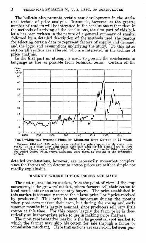
The purpose of this bulletin is to provide a basis for answering these and related questions, as determined by a study of factors influencing the yearly and monthly price variations over a period of 20 years. This period includes years in which the price situation has been somewhat comparable with the present ; in fact, years of record production and depressed prices have occurred with more or less regularity at least during the past half century. The alternating ups and downs in cotton prices since 1890 are illustrated in Figure 1.

^The author is indebted for assistance in preparing the first part of this bulletin to Louis H. Bean, of the Bureau of Agricultural Economics, and Edmund M. Daggit, of the American Cotton Growers' Exchange, who until recently was with the Bureau of Agri- cultural Economics. Since the author left the bureau in early 1926 they have done much of the diflacult work of revising the original manuscript. They suggested the first part and contributed freely in its preparation. The assistance of Miss Florena Cleaves, of the Bureau of Agricultural Economics, in the detailed analysis Avas invaluable.

71431'—28 1 1

TECHNICAL BULLETIN 50, U. S. DEPT. OF AGRICULTtTRE

The bulletin also presents certain new developments in the statistical technic of price analysis. Inasmuch, however, as the greater number of readers will be interested in the conclusions rather than in the methods of arriving at the conclusions, the first part of this bulletin has been written in the nature of a general summary of results, followed by a detailed description of the methods used, the reasons for selecting certain data to represent factors of supply and demand, and the logic and assumptions underlying the study. To this latter section all readers are referred who are interested in the technic of price analysis.

In the first part an attempt is made to present the conclusions in language as free as possible from technical terms. Certain of the

CENTS PER OUND

30

25

to

S

1890 1895 1900 1905 1910 1915 1920 1925

FIG. I.—MONTHLY AVERAGE PRICE OF MIDDLING SPOT COTTON IN 35 YEARS

Between 1890 and 1915 cotton prices reached low points approximately every three years. In this chart New York prices have been used for the period 1890 to 1901 and New Orleans prices 1901 to 1926. The break in the curve in 1914 represents the period during which cotton exchanges were closed on account of the declaration of war.

detailed explanations, however, are necessarily somewhat complex, since the factors which determine cotton prices are neither simple nor readily explainable.

MARKETS WHERE COTTON PRICES ARE MADE

The first representative market, from the point of view of the crop movement^ is the growers' market, where farmers sell their cotton to local merchants or to other country buyers. The price established in this market is commonly termed the " farm price," or " price received by producers." This price is most important during the months when producers market their crop, but during the spring and early summer months it is largely nominal, since producers sell very little cotton at this time. For this reason largely the farm price is theoretically an inappropriate price to use in making price analyses.

The most representative market is the large central spot market to which the farmer may ship his cotton for sale through a factor or conmiission merchant. Here transactions are carried on between pur-

FACTOKS AFFECTING THE PBICE OF COTTOÎT 6

chasers representing mills, exporters, and other interests, on the one hand, and commission merchants and factors or others on the other. Such spot markets are located at advantageous points throughout the Cotton Belt. Probably the most representative is New Orleans.

Two of these spot markets, New York and New Orleans, as well as Chicago and certain foreign markets, have future exchanges, where contracts are entered into for the delivery of cotton of standard grades and in standard quantities in specified future months for specified prices. These prices are the familiar " futures " prices and are identified by the particular month in which delivery is to take place. New York is the most important futures market in this country and Liverpool the most important one in the world.

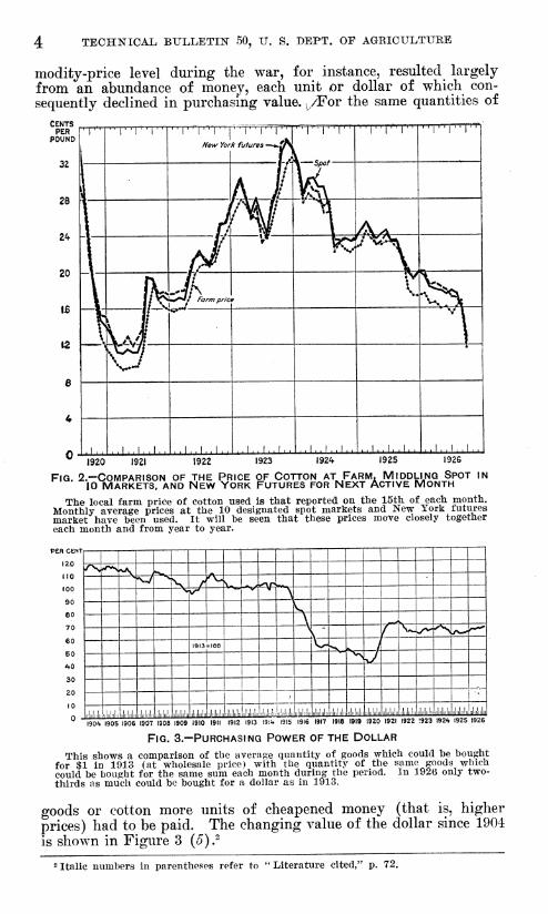
The price of cotton is determined largely in the futures markets, although the spot situation may be and often is an important factor. Since cotton may be sold or bought for delivery in future months, a purchaser, in effect, can place his order for his future needs and a seller can provide for the disposition of his cotton when it becomes available. In the meantime an operator can buy from one and sell to the other, thus evening up the operation. In case the price for future delivery goes much higher than the current price the operator buys the cotton in the spot market and sells it for delivery in the future month at the higher price, carrying the cotton over the intervening period. The continuation of this process tends to bring the prices together. A similar purchase in one market and simultaneous sale in another, known as a straddle between markets, tends to keep prices in the two markets within a margin equal to the cost of transportation between them. As a result, all the prices at the central and futures markets, as well as at the local farm markets, tend to move together, both as between markets and between months for future delivery. (Fig. 2.) Since it is in the futures operation that antici- pated needs are met, and since, by the mechanism of straddles, such needs are averaged out and communicated to the spot markets, it may be said that the futures markets determine the prices. A fuller discussion of the mechanism of prices is given elsewhere in this bulletin (pp. 30-32).

EFFECT OF SIZE OF SUPPLY UPON PRICE AND VALUE OF CROP

It is commonly understood that a large crop of cotton brings a low price and a small crop a high price, but the mathematical relation between the size of the crop and the resulting price is not usually known. For example, what change in the average annual price would be likely to result if the size of the crop were increased from 12,000,000 to 14,000,000 bales? To answer this question it is necessary first to take account of another important factor which has been found to have an important influence on changes in price from year to year—^the general level of commodity prices. When prices of other things go up there is a tendency for cotton prices to go up with them ; when other prices go down there is a tendency for the price of cotton also to go down. This was well illustrated by the general rise in prices during the World War and the general decline in prices after the war, and may be explained on the ground that a change in the general commodity price level means a change in the value of money with which cotton is purchased. The high com-

TECHKICAL BULLETIN 50, U. S. DEPT. OF AGRICULTURE

modity-price level during the war, for instance, resulted largely from an abundance of money, each unit or dollar of which consequently declined in purchasing value. ,/For the same quantities of

CENTS PER

POUND

32

28 •

2A.

20 -'

\2

'1" "I'T'I" ..,,,r,rr,,,|r'T"|"|"|"l"l"l" /^etv York futures -~*-&\

1 \\ , .

"l"l"l" " 1 " 1 " 1"'^

H \ J

\\ A^

(^

V V: \

h *^^f Farm prie ? \ ^ \ J 1 \5

-aij^ MIMIMIM MIMIMIM MIMIMIM MIMIMI,, .,I.,I..IM MI. JMIM 1924 1925 1926 1920 1921 1922 1923

FIG. 2.—COMPARISON OF THE PRICE OF COTTON AT FARM, MIDDLING SPOT IN 10 MARKETS, AND NEW YORK FUTURES FOR NEXT ACTIVE MONTH

The local farm, price of cotton used is that reported on the 15th of each month. Monthly average prices at the 10 designated spot markets and New York futures market have been used. It will he seen that these prices move closely together each month and from year to year.

PER CENT 120 7s! -'^ '^. i*^_ MO ^ ̂ ^

V / i^^ N«^ •Y^ 100 X \X "A 90 V 60

\ , f^ 70 \

\ (— V. \y^ ̂ s r>~^ r^

60 1913 = 100 vj ̂ . «s_ Í

60 S \J ¿Í-0

30 _^,_ 20

ululiiji alula ulululu iiliilir iihl'lii ,||l,,!, '|!|'lii!i llililliil iiMiili lllllllll! {!i!l!llll üliiliili lil.iliilii „|;,|,;!„ MAX lllüllllll |!llllll!ll IIIMIIIIII

0 - 130^ 1905 1906 1907 1908 1909 1910 1911 1912 1913 I9Í4 1915 1916 1917 1916 1919 1920 1921 1922 !923 I92ÍI 1925 1926

FIG. 3.—PURCHASING POWER OF THE DOLLAR

This shows a comparison of the average quantity of goods which could be bought for $1 in 1913 (at wholesale price) with the quantity of the same goods which could be bought for the same sum each month during the period. In 1926 only two- thirds as much could be bought for a dollar as in 1913.

goods or cotton more units of cheapened money (that is, higher prices) had to be paid. The changing vahie of the dollar since 1904 is shown in Figure 3 (5)?

2 Italic numbers in parentheses refer to " Literature cited," p. 72.

FACTORS AFFECTING THE PRICE OF COTTOK

If the influence of this factor—^the general level of commodity prices—is removed from the price of cotton, a fairly deñnite relationship can be established between the price of cotton thus adjusted

CENTS PER POUND

UO L

\

35 \ \

\ =RICE -SUP 1

PLY CURVE , 30 \

\

25 \ V \ <

20 \ v_ N S^

15

10

S

^ ^

./ "^ -^

1 1

( PRICE ADJ 1

1 1 1 JSTEO TO PRICE LEVEL OF 150 )

1 1 I

0 J _ MILLIONS

OF DOLLARS

1,750

1.500

1.250

1.000 1

\ V V ̂

X.

VALL E-SU :>PLYC ,URVE

^^ ^

■--

'^'•^*..

j

■^,11, '

■--

0 1 1 ! 2 1 3 1 ̂ 1 suppn

5 1 f IN M

5 1 LLIONS OF SA L' 9 2 0 2 I 2 2 2 3 2^

FIG. 4.~RELATION OF THE SUPPLY OF COTTON TO PRICE AND VALUE

Prices and values are adjusted to a current price level of 150—that is, 50 per cent higher than in 1913. If there is no change in general commodity prices a given change in supply produces a somewhat greater change in price, so that a larger supply tends to sell for less than a smaller one. This chart is based on December prices and supply data for 1905 to 1924.

and the size of the supply. In Figure 4 this relationship is shown. The horizontal measurements are the size of the supply in millions of bales ; the vertical measurements are the New Orleans prices of cot-

6 TECHKICAL BULLETIN 50, U. S. DEPT. OF AGEICULTUEE

ton in cents per pound in December, adjusted to a commodity price level 150 per cent of the average prices in 1913—approximately the level in 1926-27. The curve in the body of the chart traces the relationship between these two. Thus for a supply of 12,000,000 bales the price of cotton at current commodity price levels would normally be about 30 cents per pound. If we multiply the price per pound times the number of pounds in the supply (12,000,000 times 478) we obtain for the value of 12,000,000 bales supply approximately $1,700,000,000. On the other hand, with a supply of 18,000,000 bales, the price would be about 15 cents per pound and the value of the supply would be $1,300,000,000. This means, other things being equal, that the larger the supply the less the value of that supply. The value-supply curve shown in the figure was secured, as just illustrated, by multiplying the market price for given supply figures by the supply in pounds. This value-supply curve shows a consistent downward trend as we go from small supplies to large supplies. Relationships similar to that shown in Figure 4 obtain also between supply and the yearly average price at the central market or at the farm.

This relationship between the size of the supply and the market value of the supply has an important bearing upon the amount of money that producers will receive for their crop, for the largest element in the supply for any given season is the crop/^The other element is the carry-over at the beginning of the jear^iî the carry- over is 2,000,000 and the producers raise a crop of 16,000,000 bales, the supply would be 18,000,000 bales, the price would be about 15 cents, and the value of the 16,000,000-bale crop would be 0.15 X 478 X 16,000,000, or approximately $1,150,000,000. If, however, the crop were 10,000,000 bales, the supply would be 12,000,000 bales, the price would be 30 cents, and the value of the 10,000,000-bale crop would be 0.30X478X10,000,000, or approximately $1,430,000,000. Evidently it would be to the interest of producers to raise the small crop. They would get 25 per cent more money for it and their producing and harvesting costs would be less. Their profits would be much greater.

The significance to producers' gross income of this relationship between size of supply (chiefly crop) and value of supply has been amply illustrated during the past seasons, as shown by the figures in Table 1.

TAHLE3 1.—EeHaUonsMp 'between si^e cmd value of cotton crop

Year

Cotton production in United States

Average price

received by producers

Gross income

1924

Million bales 13,628 16,104 17, 977

Cents 23.0 19.5 12.4

Million dollars

1,567 1925 1,570 1926 ... 1.115

The increase in production of 5,000,000 bales from 13,600,000 to 18,600,000 in 1926, resulted in a decrease in income of more than $500,000,000. The larger crop in 1925, however, though bringing a

FACTOKS AFFECTIÎTG THE PRICE OF COTTOiT 7

lower price, sold for the same amount as the smaller crop of 1924^ largely because of improved commodity price levels. But the 1925 crop, being in excess of consumption, increased the stocks on hand at the begmning of the 1926-27 season. Consequently the addition of another large crop in 1926 to a plentiful carry-over reduced the average price from 19.5 to approximately 12.4 cents and the value of the crop from $1,570,000,000 to about $1,115,000,000.

FACTORS AFFECTING CHANGES IN COTTON ACREAGE

Since there is a definite tendency for smaller cotton crops to sell for more than larger crops, it may be asked why larger crops con- tinue to be produced; why, in other words, the annual supply does not tend toward smaller rather than larger quantities if smaller crops are more profitable to the farmers as a group ?

The answer is that the interest of the individual producer is op- posed to the interest of the producers as a group. Thus, if producers as a group should produce smaller crops the price would be higher and it would be to each individual's interest to produce as large a crop as possible to take advantage of the higher price. But these two points of view could be reconciled if producers knew what the prices were going to be when they marketed their crops and were guided by them rather than by the prices at the time they are making their plans for the coming season. Thus, when prices are high in December and January producers tend to plant large acreages and raise large crops, but when these crops come on the market they tend to depress the price to levels which render the year's efforts unprofitable.

Not only are the differences between individual and group interests and the lack of foresight in planning production responsible for the production of crops too large to be profitable, but variations in yield, largely uncontrollable, often result in large crops. Large yields per acre, however, are not so detrimental to the producer if they are raised on small acreages, for the small-acreages mean lower total costs so that the production is profitable despite its size. Large crops on large acreages, with somewhat smaller yields per acre, tend to be unprofitable, for total costs are large and total value is small. It is apparent, therefore, that acreage is in a large part at the root of profits to the producer and that proper control of acreage would do much to stabilize prosperity in the Cotton Belt. For this reason a study of the relationship between factors already determined in any given year and acreage changes in the following year is of particular significance.

The price of cotton is a dominant factor in determining the acreage planted the following year, as can be demonstrated by comparing ^ prices of cotton relative to prices of other farm products in January with acreage during the following season. The comparison is brought out more sharply if the changes in acreage from year to year are compared with the changes in relative prices from year to year. Thus, if the average spot price of cotton in New York during January is divided by the corresponding Bureau of Labor Statistics Index Number of Farm Products for a number of years and the changes in this relative price from one January to the next January

8 TECHíí^ICAL BULLETIJÍ?^ 50, U. S. DEPT. OF AGRICULTUEE

are plotted on a graph which also shows changes which take place in the acreage from year to year a very close coincidence is found, as may be observed in Figure 5.

190^ '06

FIG. ö.—CHANGES IN PRICES OF COTTON FROM JANUARY TO JANUARY AND CHANGES IN COTTON ACREAGES HARVESTED FROM YEAR TO YEAR

Since 1904 the acreage in cotton has usually been reduced when prices in Jan- uary were lower than in the preceding January and increased when prices were higher.

♦ lO

-10

•20

0 —f—1-T!

1902 '04 '06 '08 '10 '12 '14 '16 '18 '20 '22 '24 '26 '28 YEAR OF HARVEST

FIG. 6.-ACTUAL PERCENTAGE CHANGES IN COTTON ACREAGE HARVESTED COM- PARED WITH CHANGES AS ESTIMATED

Changes in cotton acreage during the years 1902 to 1926 have been largely determined by the price of cotton, by the general level of other farm-product prices in the preceding year, and by the change in acreage of the preceding year.

This usual response of cotton growers to changes in prices can be utilized in forecasting changes in cotton acreage. This is demonstrated elsewhere in this bulletin (see p. 19) where a detailed analysis of the relationship of cotton acreage to prices and other factors is presented. From this analysis it appears that cotton prices during

FACTOBS AFFECTIISTG THE PRICE OF COTTOK 9

December in relation to prices of other farm products and the changes in acreage made in the same year largely explain the changes in acreage the following yearr Estimates of acreage changes made from these factors from 1903 to 1926 were very close to the actual increases or decreases, explaining more than 90 per cent of the actual changes made by farmers. These estimates and the actual acreage changes are shown in Figure 6.

As of pertinent interest in the cotton situation of 1926-27 it may be noted that the maximum reduction during the period 1903-1926 has not exceeded 14.7 per cent and the cotton price at the time of preparation for planting being around 12.4 cents, indicated an acreage decrease of some 10 per cent in 1927 as compared with 1926. It is to be observed that such a reduction, as indicated by the analysis, was based on the assumption that farmers would make the usual response to low prices and did not take into account the possible results of an effective acreage-reduction campaign.

FACTORS INFLUENCING MONTHLY PRICES OF COTTON

In analyzing the monthly fluctuations in cotton prices it was found desirable for the sake of completeness to take into account more factors than were used to explain the rather simple relationship between prices and supply from year to year. According to economic theory, price results from the balancing of demand and supply. Demand and supply are each made up of numerous factors of varying importance. Variations in cotton prices can largely be explained by a few well-selected factors. Among these few the factors of supply are found to be of greater influence than factors of demand, as the foregoing discussion of price-supply relationships on an annual basis would lead one to believe. The greater influence of supply factors appears obvious from the fact that changes in the basic demand for cotton, arising from the growth of population, and changes in the needs and buying power of consumers vary comparatively little from ijaonth to month and from year to year, whereas extreme variations in supply are frequent. Furthermore, despite much adverse criticism of crop reports, but chiefly because of these reports, it is much easier for the market to gauge and measure changes in supply than for it to measure changes in demand.

Numerous factors of demand and supply have an influence upon the price of cotton, but it is not possible, nor in fact necessary, to take all factors into account. About 90 per cent of the variations in monthly prices of cotton over a period of 20 years can be explained by factors represented in eight series of data. Other, and more numerous, factors than those selected might have been used, but they would not have afforded an appreciably better explanation of the fluctuations in prices, largely because the inclusion of more factors would have been, for statistical purposes, essentially a repetition of what was already included. For example, a series showing the takings of mills does not differ materially from a series showing the mill consumption. The series which were selected, classified as to whether they were considered as demand or supply factors, are presented as follows:

Supply factors: (1) The indicated, or actual, supply of cotton in the united States at the beginning of the month. (2) The " potential " supply, or estimated size of the crop.

10 TECHNICAL BULLETIN 50^ U. S. DEPT. OF AGKICTJLTURE

Demand factors: (1) Relating to consumption: Accumulated domestic consumption, by months. ^Accumulated exports, for foreign consumption, by months. (2) Relating to business conditions: Accumulated rates of change in general price level. "'Average price of industrial stocks. (3) General: Series representing the years from 1903 to 1924 and indicating yearly changes, or " trend," in demand and other trend factorSi^ Series representing the months of the crop year, beginning June, and indicating seasonal changes not otherwise taken care of.

The relationship of each of these factors to the price of cotton will be discussed in turn.

INFLUENCE OF SUPPLY UPON PRICES

A comprehensive statement of the relationship of market concepts of supply to price is given on pages 30-32. An explanation of the reasons for selecting the particular measurements of actual and potential supply used is here presented. It is sufficient to state that actual supply for any given date is taken as the carry-over in the United States at the beginning of the season plus the ginnings and imports up to the given date and minus the exports and consumption up to the given date. It is, in short, the ginned cotton in the country which is available for export or consumption on the given date. This measurement of supply must not be confused with the measurement used in analyzing the relationship between annual supply available and price from year to year. In that case the total crop was added to the carry-over to give the supply figure.

Potential supply for any given date is taken as the current estimate of the size of the crop, except that from January to July it was found that the best results were secured by using the size of the crop in the last year as a measure of potential supply for the coming season. This was justified on the hypothesis that, failing more accurate information, the last year's crop is a more important factor than the market opinion of next year's crop. It was also justified by the greater success in explaining price fluctuations when this was used than when other measurements were used. Both actual and potential supply were expressed in bales, usually millions of bales.

Before going into a detailed description of the month-to-month relationship of supply to price it is interesting and useful to consider the changes which take place in both the actual and the potential supply series as we pass through a large crop year and to note the corresponding changes in price which take place as a result.

As the season develops in a large-crop year the market becomes cognizant of the large crop through the medium of crop reports issued both by private concerns and by the Government. "Poten- tial " supply becomes larger. Price should become lower. Some- what later, when the crop begins to pass through the gins in quantity, the expectation of a large crop is verified, and the actual supply becomes larger, thus tending to support and augment the influence of the large potential supply in causing prices to decline.

In such cases it would be logical to expect the price toward the end of the season to be considerably lower than at the beginning. But if, as the season approaches its termination, the next crop seems to be a small one, and is expected to be a small one by the market, the

FACTORS AFFEOTIIí^G THE PRICE OF COTTON" H

new potential supply is smaller, and at the same time the actual supply is being diminished by consumption and exports, both of which are stimulated by the lower prices. A recovery in prices is then to be expected.

On the other hand, if the next crop seems to be another large one, the potential supply is of sufficient size and influence to keep the price at low levels. This characteristic movement of price resulting from changes in the supply can be nicely demonstrated by classifying years of large crops into those followed by years of large crops and those followed by years of small crops and noting the movement in prices that takes place during the two types of years.^ This movement is shown in Figure 7.

The changes in prices during each of the selected years which comprise the averages in Figure 7 (upper section) are shown in Figure 8 to illustrate the extent to which the situation in any one year of large production may differ from the general statements in the preceding paragraphs {28),

In the more analytical study of month-to-month relationships of supply and other factors to price it was found desirable to use a " world " price of cotton, which needs some explanation. The price of middling spot cotton at New Orleans, average for the month of closing quotations, is used, adjusted, or corrected for variations in the levels of prices here and abroad and corrected for variations in the British exchange rate.

Just as it was necessary to adjust the annual price of cotton to a constant price level, in order to eliminate the effect of the general level of prices, it is likewise necessary to make the same adjustment in the monthly prices; and since roughly about half of our cotton is exported it is also necessary to make a similar adjustment to eliminate the influence of the foreign price level upon the price of cotton. The rate of exchange is an additional factor which must be allowed for. Great Britain is our most important foreign market for raw cotton, and many of the purchases from other countries are also made in sterling exchange. When British money becomes more valuable—when the rate of exchange in terms of dollars rises—^it means that the buyer in Great Britain can obtain more cotton for the same quantity of British money and the foreign demand for cotton will appear to the American to have increased. The New Orleans spot price corrected for variations in the general levels of commodity prices, here and abroad, and for the variations in sterling exchange, may properly be termed an adjusted world relative price.

The relationship of the actual supply and the potential supply to the price of cotton changes from month to month through the season. In both cases an increase in supply tends to cause a decrease in price, or vice versa; but the decrease in price resulting from a given increase in either the actual or potential supply may be much greater at one part of the season than at another. The potential

3 p. K. Whelpton, in Seasonal Fluctuations in the Price of Cotton (36), classified years according to whether the price is high in October or not, and traced a characteristic movement in subsequent prices. Perhaps this " seasonal " movement he found can be explained on the basis of the changing supply described above and in the normal relation between supply and prices.

12 TECHNICAL BULLETIN 50, U. S. DEPT. OF AGKICXJLTUEE

supply has its greatest influence upon prices during the fall months, when prospects for the crop become more and more definite and forecasts of production are being made at frequent intervals.

PER CENT OF YEARLY AVERAGE

110

100

90

80

\ J \ YEARS OF LARGE CROPS / \ ê \ ê \ / \ /

1 ê . ê V é \ / ►^ X > V

\ X L-^ Followed btj large crops ^'' \ X ^^ ^ 1 ^ V % V / % ^ / S , „ ■/,„ '% X / \ ^^ *^^ ^ \ \ 1 \à «i^ y

'--. .."' ^

\ _^rf /" \ -V, ollowed by smc ill crop. 3

AUG. SEPT. OCT. NOV. DEC. JAN. FEB. MAR. APR. MAY JUNE JULY

no

100

90

80

YE :AR5 0 F SMAL L CRO PS

Follov\> 'ed by large c rops ^

>^ \ _ ^4 __ ,-'-'

./■

i \^^—' ^ j^r' rs.i_^ X /

y, r Followed by small crops

f

AUG. SEPT OCT. NOV. DEC. JAN. FEB. MAR. APR. MAY JUNE JULY

FIG. 7.-PRICES OF COTTON IN YEARS OF LARGE AND SMALL CROPS

When indications are that a large crop will be followed by a small one, or a small crop by another small one, prices tend to rise during the spring months, but when a large or small crop is likely to be followed by a large crop, prices tend to decline during the spring months.

The actual supply, determined from stocks, ginnings, consumption, and exports, has its greatest effect upon prices during the latter

FACTORS AFFECTING THE PRICE OF COTTON 13

PER CENT OF

YEARLY AVERAGE

120

- YEARS OF LARGE CROPS FOLLOWED BY YEARS OF SMALL CROPS

//

-

\ \ \ N \

'--.

1 ===== Aver age

)4 74 06 78

/ i **v /)¿JÍ' /\ 110 •t*«**«**»* I9(_ <j^

\ \

k N

ß- 7^ i

/

100 ■

90

\ \ \ \

\

""""'

::^ \

¡/ rfl^"«— 0 / / / / / y /

-

>< / -

60

\ \ / \ *

100

YEARS OF LARGE CROPS FOLLOWED BY YEARS OF LARGE CROPS

AUG. SEPT. OCT. NOV. DEC. JAN. FEB. MAR. APR. MAY JUNE JULY

FIG. 8.—PRICES OF MIDDLING SPOT COTTON AT NEW ORLEANS IN YEARS OF LARGE CROPS

There is a considerable difference between the behavior of cotton prices during the years of large crops, but there is a general tendency for prices to rise or to decline during the last half of the season, depending upon whether the prospects are for a small or a large crop the following season.

14 TECHIsriCAL BULLETIN 50, U. S, DEPT. OF AGEICULTUEE

half of the crop season when the size of the current crop is rather well known, stocks are decreasing, the size of the next, " potential," crop is uncertain, and the rate of consumption is of more immediate interest.

In general it may bç said that the actual supply affects prices throughout the year, ^'Vhile potential supply has a diminishing though little effect on price between January and July, inclusive. " For a graphic representation of these relationships see Figure 14.

INFLUENCE OP DEMAND UPON PRICES

The basic motives controlling demand are simple; their effect on price is very complex. Obviously the demand for raw cotton depends ultimately upon the quantity that final consumers of cotton goods will purchase at various prices. Obvious, also, is the fact that both domestic and foreign consumers of American cotton and cotton goods are induced to buy larger quantities when prices are low but buy smaller quantities when prices are high. These usual reactions to changes in prices do not, however, indicate changes in demand. A true measure of demand must explain changes in consumption with no change in price, or, conversely, changes in price with no change in consumption. An increase in demand may be said to take place when more cotton is purchased at the same price or when the same amount is purchased at a higher price.

Changes in demand depend upon the continually changing wants of consumers and upon changes in their ability to satisfy those wants. In an analysis of cotton prices it is therefore necessary to make use of data that will represent changes in these two factors— the wants of consumers and their purchasing power.

On the assumption that the quantity of goods already possessed (among other things) determines the wants of consumers for more goods, an indirect measure of the supplies of cotton possessed by all classes of consumers was developed m this study, since direct measures were not available. Among the different classes of consumers are spinners, manufacturers, wholesalers, jobbers, retailers, and the ultimate consumers of cotton goods. All of these agencies carry stocks of varying sizes, in anticipation of future needs, and all such stocks have an influence upon the price of raw cotton in the central market, ^his indirect measure of domestic stocks, and thereby of demand, is termed the accumulated domestic consumption of cotton. A similar measure of stocks in foreign countries is termed the accumulated exports of cotton.

Headers who are interested in the details of these accumulated raeasures of stocks and the various economic and statistical assumptions which they embody are referred to page 32. For an under- standing of their relationship to price it will be sufficient merely to state that they were compiled from monthly data on domestic consumption and exports of raw cotton, and that for any given month the accumulation represents an average accumulation or sum of the monthly consumption or export figures—an average annual figure— for three years ending with the given month in which the most recent year is considered of greatest importance, the second year of less importance, and the earliest year of least importance.

FACTOES AFFECTING THE PRICE OF COTTON" 15

These indicators of the amounts of cotton in domestic and foreign channels of consumption are shown in Figure 8. They illustrate (1) the great expansion in foreign takings of American cotton before the World War, the contraction during and after the war, and the more recent increased purchases to make up for the previous curtail- ment; and (2) the increased consumption in the United States during the war and a continuation of the upward trend since 1921.

In their relation to price both of these measures of cotton in consuming channels show that within certain limits an increase in the quantity that has already gone into the channels of final consumption tends to lower prices, and vice versa. (See fig. 16.) In the case of domestic consumption an increase beyond 6,000,000 bales appears to have no additional effect on price; in the case of exports an accumulation in excess of 7,000,000 bales appears to have

BALES MILLIONS

uiiUáiULliuUukLJ^^^ LIHI I i,i„l Lii-i>.l„ili.iLiJui,J Li.ii.Li,.i.i„l |,jJni,,[|.ilL.i.hL.i,i,.l,j,j,,il.,|,j,,l,,i,,l,|..L,l.i,.L,, 1902'03 '04 'OS '06 "07 '08 109 '(0 Ml '12 '13 '14 '15 '16 '17 '18 '19 '20 '21 '22 '23 '24 '25 '26 '27 '2Ö

FIG. 9.—UNITED STATES COTTON CONSUMPTION AND EXPORTS

Foreign countries increased their purchases of American cotton before the World War, curtailed purchases during the war, and since then have been replenishing. Consumption in the United States increased during the war and has maintained an upward trend since 1921.

no further influence on price, indicating that accumulations beyond this point are noninfluential to any additional degree.

On the other hand, a decrease in accumulated consumption below 4,500,000 bales and in exports below 5,000,000 bales appears to produce no further increase in price; this situation runs counter to expectation. Very restricted use of cotton in past years should mean that available consumer supplies were exhausted and that further purchases were imperative. But probably the high prices following such a situation have served to stimulate more production before such low accumulations have opportunity to exert an emphasized effect. The expected price influence is thus probably reflected in the supply-price relationships, which reflect current situations with greater promptitude than do the three-year accumulations.

INFLUENCE OF PURCHASING POWER OF CONSUMERS

The willingness of consumers to pay for goods which they want depends in a large measure upon their purchasing power, which in

16 TECHlSriCAL BULLETIN 50, U. S. DEPT. OF AORICtTLTURE

turn depends upon such specific conditions as the state of employment of consumers and the level of wages earned. Inasmuch as the economic well-being of consumers is directly related to business conditions in general, and more particularly to industrial activity, it may, for the purposes of this study, be represented by a series of data which are either a direct or an indirect measure of business activity.

Investigators of the relationship between changes in the general price level of commodities and business conditions have found that^| changes in the former reflect to a high degree changes in industrial activity, provided fluctuations or rates of change in current months as well as during a preceding period of a year or more are taken into account and changes in recent months be taken as of greater importance than those of earlier periods. (Fig. 10.) (For further discussion and method of construction see p. 40.)

This indirect measure of business activity, termed the accumulated rate of changes in the general commodity price level, possesses a qualification as an indicator of demand not possessed by direct meas-

1902 "03 "04 'OS '06 '07 -08 10 "11 '12 '13 'K '15 '16 '\7 '18 '19 '20 '21 "22 '23 '24 "25 '26 '27 '28

■i

FIG. 10.—ACCUMULATED RATE OF MONTHLY CHANGE IN WHOLESALE COMMOD- ITY PRICES AND INDEX OF INDUSTRIAL EMPLOYMENT, UNITED STATES

These changes tend to reflect, among other things, the variations in industrial employment and consequently the purchasing power of the wage-earning portion, of consumers.

ures of current business conditions. It may be taken to serve as an indication of probable as well as current changes in the purchasing power of consumers, which is undoubtedly considered by those who carry on transactions in the cotton markets with a view toward later resale and who thereby bring into the current price of cotton the effect of expected changes in consumers' purchasing power.

The degree to which such an index of price changes reflects fluctuations in industrial employment and consequently the purchasing power of that portion of consumers represented by factory wage earners is shown in Figure 10.

As indicated by this accumulated rate of change in the price level, declining business conditions and therefore lower purchasing power of consumers, appear to have a greater effect upon the price of cotton than does increasing business activity. Stated in another way, the decline in cotton prices which accompanies a given accumulated decline in the general price level is generally about twice as great as a rise in the price of cotton which accompanies an accumulated price level rise of the same amount. (See fig, 18.)


The effect of business conditions and the purchasing power of consumers just described deals with the basic demand for cotton goods. Inasmuch, however, as the market price of cotton is determined largely by purchase with a view to reselling, it is necessary to consider the effect on price exerted by the buyers' idea of what the reselling price may be. This conception may relate to prospective general business conditions or to prospective conditions in the textile industry, since these affect the buying power of final consumers and the demand by manufacturers of cotton goods.

A common basis for such conceptions of future developments is / the trend of stock prices, which in the past have often forecasted changes in industrial activity, employment, and wage payments, factors bearing directly on the purchasing power of consumers as well as on the probable demand for cotton for industrial consumption. Prior to 1913 prospective business conditions, as represented by the Dow-Jones average of 20 industrial stocks, appear to have had no recognizable effect on cotton prices. During the years 1913-1918 stock prices falling below 80 tended to be accompanied by low cotton prices, and during the postwar period a similar depressing effect on cotton prices appeared when stock prices were below 100. From this it may be concluded that in the more recent years business conditions as reflected in low stock prices tended to depress the price of cotton, whereas business activity as shown by high stock prices failed materially to increase it. (See fig. 17.)

In addition to the effect on price of the specific demand factors - already presented there are other changes in cotton prices that are due to the gradual and constant increase in demand induced by the growth of population or by the development of new uses for cotton.

Prior to the war there appears to have been a constant increase in the demand for cotton such that the same quantity which sold for a world relative price of 0.9^ in 1906 would have sold for about 1.2^ in 1913, provided other price-influencing factors, such as business conditions and price levels, were also the same in the two years. (See fig. 19.) Except for a falling off in that demand during the period of the World War, it has since then continued to increase relative to the cost of production, so that at the present time a supply which in 1906 sold for 0.9^ would sell for approximately 1.5^, an increase of about 70 per cent, due largely to the mere growth of population.

RELATIVE IMPORTANCE OF SUPPLY AND DEMAND FACTORS IN COTTON PRICE FLUCTUATIONS

The two factors of supply (actual and potential) and the four ¿/ factors representing demand (domestic consumption, exports, industrial stock prices, commodity prices and changes in the annual and seasonal demand for cotton) when taken together over a period of 20 years, explain practically all of the monthly fluctuations in the price of cotton. This is illustrated in Figure 13, where the dotted line represents the price of cotton as estimated from the several factors shown in Figures 6-12, taken together, and the solid line • shows the actual monthly average price. Except for two or three brief periods during the 20-year interval from 1905 to 1925, there is a remarkable closeness between the estimated and actual prices.

71431°—28 ^2

18 TECHISriCAL BULLETIN" 50, tJ. S. DEPT. OE AGEICULTURE

Inasmuch as the estimated prices are derived entirely from the usual relationships between the several factors and price, it may be said that they account for most of the changes that have taken place in cotton prices since 1905. Measured mathematically, these factors explain about 90 per cent of the fluctuations illustrated in Figure 11.

The supply factors are usually responsible for about 39 per cent of this amount; the factor representing the long-time growth in demand is responsible for 26 per cent, while the more variable demand factors are responsible for 25 per cent. With changes in supply from year to year and month to month, thus shown to be the most important influence in cotton prices, it is obvious that less violent price fluctuations would result were the changes in production less violent.

1905 '06 '07 '08 '09 '10 'II '12 '13 '14 '15 '16 '17 '18 '19 '20 '21 '22 '23 '24 '25 '26 '27

FIG. 11.—ACTUAL PRICE OF MIDDLING SPOT COTTON, NEW ORLEANS, AND PRICE ESTIMATED FROM FACTORS OF SUPPLY AND DEMAND

More than 90 per cent of the monthly fluctuations in the actual price of cotton can be accounted for by the several factors of supply, domestic and foreign consumption, the general commodity price level, and business conditions, as indicated by the closeness of prices estimated from these factors to the actual prices from 1905 to 1925.

STATISTICAL ANALYSIS OF FACTORS INFLUENCING COTTON / PRICES

From an economic and statistical research point of view, the purpose of the study presented in the following pages is threefold : (1) To determine the factors which influence the price of cotton, (2) to reduce these factors to numerical measurement in so far as possible, and (3) to find and define the statistical relationship, if any, existing among these factors and the price. The study is not primarily an attempt to develop methods of forecasting, but rather an attempt to define quantitatively those relations of various factors to price, the qualitative nature of which is in many respects generally understood. For example, it is well known that a decrease in supply will bring about an increase in price. But an accurate statement of the percentage change in price accompanying any given percentage change in supply can not be made without defining the quantitative relationship between the two. This type of analysis is also a logical prerequisite to quantitative forecasting of price, for of what benefit

FACTORS AFFECTING THE PRICE OF COTTOK 19

in forecasting price is it to know what the supply will be unless the price effect of that supply is also known ?

Although this study is intended to analyze concurrent relationships rather than to produce forecasting methods, nevertheless in the process of constructing measurements of potential supply certain methods of forecasting acreage were developed. The use of forecasts of acreage in the measurement of potential supply did not prove to be successful, but the acreage forecasting methods in themselves are of sufficient interest and significance to justify their presentation as a unit in this study.

The analysis of the relationship of price to various factors as here described divides logically into two sections. The first section deals with price-supply relationships from year to year in an attempt to explain the annual variations in price. It is concerned with fejver variables and is much simpler than the more ambitious analysis described in the second section which attempts to explain the month-to-month variations in price on the basis of systematic relationship to several sets of factors for a period of 20 years. For convenience in referring to them, these two sections may be termed the "preliminary analysis" and the "detailed analysis." The preliminary analysis consists of two unit studies, the results of one of which have been presented in the preceding pages of this bulletin. The methods employed in both cases were those of linear multiple correlation (16)^ applied to the logarithms of the variables. In the detailed analysis curvilinear multiple correlation methods were applied to the original variables.

Pioneer work somewhat similar in nature to that described in this bulletin has been done by Moore (5), who found that by correlating the price of cotton with the production and the price level a relationship evidenced by a multiple correlation coefficient of 0.859 existed. Since this work was done, however, statistical methods have been developed which permit of a more comprehensive analysis of the price-factor relationships involved.

METHODS OF FORECASTING ACREAGE

In an earlier publication (11) the author has presented in considerable detail the theory underlying the use of prices in forecasting the acreage of cotton and set forth a statistical method for performing this forecasting. In subsequent publications {10, 15) further dis- cussions and more refined statistical technic were presented. The present description is essentially that given in a paper ^ presented at the December, 1926, annual meeting of the American Statistical Association.

If prices of cotton relative to other farm products are high in the late fall and early sçring when the cotton producers are marketing their crop and making plans for the new season it is logical to believe that, in the first place, the higher prices will have meant a more profitable season to cotton producers than to producers of other

* In the detailed analysis curvilinear methods of multiple correlation were employed as originally developed by Ezekiel (3). A complete description of the correlation technic may be found in Smith's Correlation Theory and Method Applied to Agricultural Research (U).

5 SMITH^ B. B. FORECASTING THE VOLUME AND VALUE OF THE COTTON CKOP. Journal American Statistical Association, December, 1927,

20 TECHNICAL BULLETIN 50, U. S. DEPT. OF AGEICULTUEE

products and, in the second place, that the higher price» will lead producers to believe that cotton will be a profitable crop to raise in the coming season—for such is the nature of the farmer. Both of these situations are conducive to expansion of acreage in the coming year. Producers who have been successful in the given year are pleased with their success and wish to increase that success in the coming year, hence they expand their acreage. Producers of other crops shift over to cotton in the hope of bettering their condition during the coming year.

From these considerations it is apparent that the price of cotton relative to the price of other farm products is likely to be a prime factor in influencing acreage changes. Accordingly, the first factor to be included in an analysis of acreage changes is such a relative price. A price which was found to give good results in past years was the average December quotation in New York for March futuBes.

To make this price series a relative price series, each average price was divided by the Bureau of Labor Statistics Wholesale Price Index of Farm Products for the corresponding month and year. The two series needed for this are shown in Table 2 in columns 2 and 3. The quotient of the price divided by the index is shown in column 4. This quotient is to be related to the acreage increase or decrease which takes place in the ensuing season. The acreage increases or decreases which actually took place and to which this series of quotients is to be related are shown in column 6. The increase or decrease is expressed as a percentage of the preceding year's acreage harvested.

Theoretically it would be more appropriate to relate the relative price to the acreage planted rather than to the acreage harvested, but the " acreage-planted '" figures are not as accurate as the " acreage harvested," nor are the deviations in the percentage of abandonment during the season large when compared with the deviations which take place in the percentage change in acreage harvested over a period of years. And, finally, it is the acreage harvested which is significant from the point of view of anticipating production.

In examining this series of percentage changes in acreage harvested it is interesting that for the period included, 1902 to 1926, according to Government estimates, there has never been an acreage decrease of as much as 15 per cent. The year in which this figure was most nearly approached was 1915, when there was an acreage decrease of 14.7 per cent from the 1914 acreage.

Not only is the price in the December immediately preceding the year of harvest likely to be significant in determining acreage changes but the price in the December two years preceding the year of harvest may also have some bearing on the acreage. For if there are two or more years of profitable growing a cumulative effect can easily be conceived of. Some producers who held back the first year that price was high, perhaps because of other rotation plans or of commitments in the form of equipment, seed, etc., may carry over the intervening year some intention to expand in cotton production. It is therefore desirable to repeat the relative price of cotton as a factor in influencing the acreage change taking, place in the given year, but in the repetition the item in the series preceding the item for the given year is employed.

FACTORS AFFECTIISTG THE PRICE OF COTTOIST 21

Yet another factor which is» desirable to employ in analyzing the change in acreage that takes place in any given year is the change that took place in the preceding year. For, other things being equal, a reaction from the change taking place in the preceding year is to be expected, chiefly because agricultural production is practically never in precise adjustment to demand, and a change in one direction in a given year is more likely than not to require a change in the other in the ensuing year, simply because an o ver adjustment has taken place. This tendency to swing from one type of change to another—a pendulum movement—^is apparent from an examination of the series showing acreage changes. Years of increase are followed more often than not by years of decrease, and vice versa.

Finally, owing to changing costs of production and changing values of farm products with reference to other products and other influences, it is easily probable that the price necessary to stimulate an acreage increase may have been gradually rising or falling through the period included in the study. Hence it is desirable to include, as a final factor in the analysis of influences affecting acreage changes, a series which represents a uniform time interval. Such a series is conveniently constructed by numbering consecutively the years included in the study, or by taking the last two digits of the calendar years designating the year of harvest.

The factors employed to explain the percentage increase or decrease in the cotton acreage of the United States harvested in a given year compared with the preceding may be summarized as follows :

(1) The New York average price of cotton for delivery in March as quoted during December of the calendar year preceding the year of harvest divided by the Bureau of Labor Statistics Index of Farm Product Prices at Wholesale for the same December.

(2) The same as (1), except that it is taken for one year earlier. (3) The percentage change that took place in acreage during the year pre-

ceding the given year of harvest (4) Trend—taken aö the last two digits of the year of harvest.

Once these series were set up, as shown in Table 2, the statistical process of analysis in this study consisted of determining the net curvilinear regression of the acreage change for the given year on the four independent factors listed above. Curvilinear multiple correlation methods cited previously were used. It may be pointed out that since values of the dependent and of relative price for observations preceding the given one were employed as independent factors all the advantages of a first-diflference method of correlation have been secured without introducing the limiting assumptions of first differences (^^). Furthermore, by introducing a trend factor as an independent factor, any possible advantages of using deviations from trend as the original series have been secured, in so far as this has a bearing upon the forecasting (18).

The net regression curves, showing the relation of each of the listed factors to cotton acreage change, are shown in Figure 12.

The first set of curves showing the relation of the relative price, one year before and two years b&iore, to acreage harvested are about as would be expected. The curve representing the relation of the relative price one year before to acreage harvested is much steeper than the other, indicating that a given change in it will produce more effect upon acreage. As a matter of fact, the curve represent-

22 TECHÍí^ICAL BULLETIN 50, U. S. DEPT. OF AGEICULTURE

ing relative price two jears before i^ horizontal throughout about half of its length, indicating that within this range it has no influence upon acreage. The curve representing the relative price

.008

+ 10

-5 -30

♦ 10

•10

•010 .012 .014 .016 .018 .02 AVERAGE MARCH FUTURE COTTON PRICE IN DECEMBER DIVIDED

BY DECEMBER INDEX OF FARM PRODUCTS

.022

-20 -10 0 +10 +20 +30 PERCENTAGE CHANGE IN ACREAGE FOR THE PRECEDING YEAR

+ H0

1902 '04 'Oe '08 •|0 '\2 '14 .'16 '18 '20 *22 YEAR OF HARVEST

•24 '26 »28 '30

FIG. I2.-RELATI0NSHIP OF PERCENTAGE CHANGES IN COTTON ACREAGE HAR- VESTED TO VARIOUS FACTORS

Net regression of changes in acreage (in percentages of the preceding year) on four other factors. These curves were used in making the estimates or forecasts of changes in acreage shown in Figure 6.

one year before becomes horizontal above a relative price of 13.5 indicating that prices higher than this can not serve to stimulate greater acreage increases. Such a flattening out of the curve is to

FACTOÈS AFFECTUSTG THE PKICE OF COTTON 23

be expected, for there are physical limitations upon the amount of acreage expansion that can take place, no matter what the price.

The curve in the second section of the chart shows the relation between acreage change in the preceding year and acreage change in the given year. It has a slope, as woum be expected—the greater the increase in the past year the greater the reaction or decrease in the given year.

The last of these curves shows the relation of the trend factor to acreage changes. From 1903 to 1912 this curve indicates an increasing increase in acreage to be normal, or, putting it in another way, should prices have remained constant during this period there would have been a normal increase in acreage of about 2 per cent in 1903, which gradually increased to a normal increase of about 5 per cent in 1912. This is probably a reflection of falling costs of production or an indication that costs of production were falling more rapidly than demand was increasing. From 1912 to 1921 there was a change in the normal annual change in acreage from an increase of about 5 per cent in 1912 to a decrease of about 6 per cent in 1921, or, putting it in another way, an increasing relative price was required to maintain a constant acreage.

This period was characterized by the rapid spread of the boll weevil throughout most of the Cotton Belt, which not only increased the unit cost of production but probably had an important psychological effect upon producers and contributed to the necessity of higher prices to maintain or stimulate acreage. It was also the period of the World War, when price relationships were generally upset. This situation terminated in 1921, perhaps because producers had become better acquainted with methods of handling the boll weevil, as is suggested by the fact that the pre-war trend in this curve was resumed.

To employ these relationship curves for the purpose of forecasting it is necessary only to obtain the values of the independents listed previously for the given year, read from the curves their effects upon acreage, and add together the resulting readings. The sum will represent the estimated or forecasted acreage change.

For illustration, suppose that in January, 1925, it was desired to forecast the percentage change that would take place in the 1925 cotton acreage compared with 1924. As shown in Table 2, column 3, the average March futures price in New York during the December just past was 23.81 cents. The Bureau of Labor Statistics (35) Index of Farm Product Prices at Wholesale was 157, as shown in column 2. Dividing the one by the other, a relative price of 15.2, as shown in column 4, was secured. Performing the same operations for the previous year gave a relative price of 24.1. From the curve showing the relation of relative price one year preceding to acreage, it was found that a relative price of 15.2 would have an effect of plus 5 per cent on acreage, as listed in column 8. From the curve showing the relation of relative price two years preceding to acreage it was found that a relative price of 24.1 would have an effect of plus 7 per cent upon acreage. The percentage change that took place in acreage in 1924, as shown in column 6, was plus 11.6. From the curve showing the relation of changes in the preceding year to changes in the given year

24 TECHNICAL BULLETIN 50, U. S. DEPT. OF AGEICULTURE

it was found that a change of plus 11.6 in the preceding year would have an effect upon the given year of minus 1 per cent, as listed in column 10. Finally, referring to the curve showing the net trend effects on acreage, it was found that in 1925 there would be an effect of plus 1 per cent. Adding together these effects, as listed for 1925 in columns 7 to 10, a sum of effects, plus 12, listed in column 11, is secured. This sum represents the estimated (or "regression estimate " of) acreage change. If similar estimates are made for all years throughout the period and these estimated changes, column 11, compared with the changes that actually took place, a very close agreement is observed. These two series, the actual and the estimated, percentage changes that took place are graphed together in Figure 6. The agreement between the tAvo is striking. The correlation (multiple correlation index) between them is 0.95; and if 1910—a bad year—is omitted, the correlation is 0.98.

It is an interesting process to deduce from the relationship curves the price of cotton at which acreage would be stabilized. Thus, for 1926 the trend influence would indicate a normal plus 2 per cent increase ; for a stabilized condition the effect of the preceding year's change (a zero change) would be plus 4 per cent. Thus, there is a combined plus 6 per cent increase to be offset by the price factor. From the price curve it is observed that a price of 11.2 would produce the requisite minus 6 per cent influence, resulting in a net effect of all the factors combined of zero change. To convert this relative price of 11.2 to a cents-per-pound price it is necessary to multiply by the index of farm products prices. This index is approximately 140. Multiplying 11.2 by 140 gives about 15.5 cents. Thus, we may con- clude that a price somewhere between 15 and 16 cents would have served to keep the acreage stabilized under conditions existing in 1926. Stating it another way, a price between 15 and 16 cents in îsTew York is one which made cotton production neither greatly more nor greatly less profitable than other agricultural enterprises in the South. It represents about the marginal cost of production plus a normal agricultural return.

PRELIMINARY ANALYSIS

RELATION BETWEEN ANNUAL SUPPLY, PRICE LEVEL, AND PRICE

In the first part of this bulletin the curves resulting from the analysis of the relation between price level, annual supply, and the price of cotton were discussed. The discussion here will therefore be largely confined to a description of the series used and methods employed.^

The available supply during a season may be considered as the sum of the carry-over at the beginning of the season and the crop harvested in the season, both with reference to the United States. It was desired to ascertain if there were any systematic relationship between this factor—supply for the crop year—and the price. But there are many factors, presumably, which influence price. In selecting a price to compare with supply, therefore, it is desirable to choose

6 This study was first presented in a somewliat summarized form by the writer in ** The Adjustment of Agricultural Production to Demand" (15).

TACTORS AFFECTING THE PRICE OF COTTOÎT 25

a price existing at a time during the year when the supply for the year would be the most important factor in making the price. Dur- ing the early part of the crop season the price is a reflection, not of what the crop actually turns out to be but of what the market thinks the crop will turn out to be. The two things are often different, as will be discussed in the detailed analysis.

To choose a price during the early part of the season for the present purpose is to compare incomparable things—a supply, as history has proved it to be, with a price determined by what the market at that time thought supply was going to be. On the other hand, to choose a price late in the season is to choose a price which is beginning to be influenced by conjectures as to the size of the next crop. A price somewhere near the middle of the crop season, when market concepts as to the size of the crop coincide with what the size of the crop actually is, should be used. This must be a price that exists some time after the crop report early in December. Because of these considerations, the average New Orleans price of middling spot cotton during December was taken as the price of cotton to which the supply, as measured by the size of the crop, plus the census estimate of the carry-over at the beginning of the season, would be related.

But even with this selection of price no systematic relationship was discoverd between price and supply because the price was affected by the movement of the general commodity price level to a much greater extent than it was affected by the changes in the supply. It was necessary to introduce an additional factor—^the average Bureau of Labor Statistics Index of All Commodity Prices at Wholesale during the corresponding December. The supply, taken as carry- over and crop, the price of cotton, and the Bureau of Labor Statistics Index were the only series of data employed in this analysis. These data are shown in Table 3.

Since it was felt that whatever relationships might be found to exist would lie between proportional changes in the three items rather than between absolute changes, the three series were converted to logarithms before correlating. Thus a constant increment added to any of the three was equivalent to a constant proportional increase. The three series of logarithms were correlated by usual multiple correlation technic in which the price, P, was the dependent, and the supply, S, and the price index, I, were the independents. The regression equation was found to be

Log P equals 1.548 Log 1-1.705 Log S-0.051,

where S is expressed in millions of bales, the price in cents per pound, and the index, as usually written, as a per cent of 1913.

The coeiScient of the logarithm of S may be interpreted to mean that the rate of change in price due to change in S is 1.7 times the rate of change in S. This means that larger supplies mean diminished values, for the value is equal to the product of S and P, and if P declines at a greater rate than S increases the product must of necessity decrease. The accuracy of the regression equation may be measured by the coefficient of multiple correlation, which in this case is 0.955.

26 TECHNICAL BULLETIN" 50, U. S. DEPT. OF AGKICULTUEE

The relationship between supply and price at any given price level may be shown graphically by substituting in the regression equation the given price-level value, letting it remain constant, while the equation is evaluated for a series of values of S. These values of S and the corresponding evaluations of the equations are a series of pairs of items which, when plotted on coordinate paper, give a curve showing the price-supply relation for the given price level in terms of logarithms. If antilogs are determined and plotted instead of the logarithms the straight line which resulted in the case of logarithms takes the familiar curvature of a price-supply curve. It was by this means that the price-supply curve adjusted for a price level of 150, discussed elsewhere in this bulletin was secured. (See fig. 4.)

To determine what size of crop will bring the maximum return to producers, the procedure might be to plot on coordinate paper the value of supply for given sizes of supply, as illustrated in the previous discussion of this point. Below this value-supply curve could be plotted a curve which represents the value of the carry-over for the specified size of supply. The difference between these two curves, of course, would represent the value of the supply less the value of the carry-over, or the value of the crop portion of the supply. The point where the difference between these two curves is greatest— where the value of the crop portion of the supply is greatest—indicates the size of supply which will bring the largest total value. With this desired size of supply known, it is necessary only to sub- tract from it the carry-over to ascertain the size of crop which will bring the producer the greatest value for that season. In general, the rule is that the larger the crop the less the value. But if the carry-over is a large proportion of the supply, larger crops, up to certain points, may mean larger values for the crop, since increasing the" size of the crop does not increase the size of the supply at as i:apid a rate.

The net regression of price on price level, 1.548, in the regression equation deserves comment. A more usual method of taking into account the influence of the price level on a given price is to divide the price by the price level. This would be the equivalent of substituting a regression coefficient of 1.000 in the equation. This, however, results in but low correlations. The regression of 1.548 means that the rate of change in the cotton price is 1.548 times the rate of change in the price level. Or, in other words, before the index of price level is a satisfactory deflator for the present purposes it must be raised to the 1.548 power. As a matter of fact, if the cotton price is divided by the index raised to the 1.548 power and is correlated with the supply raised to the 1.705 power, a correlation of —0.791 is secured which is considerably greater than can be secured by using the original index as a deflator. If from the logarithm of P is subtracted 1.548 times the logarithm of I, and if the remainders are correlated with the logarithms of S, a correlation of —0.84 results, which is the same as that secured by correlating the logarithm of (P/I^^^^) with log S, indicating that even after price has been deflated by the " stepped-up " index better results are secured by using logarithms which permit relations between proportional changes to be determined.

FACTORS AFFECTIKG THE PRICE OP COTTON" 27

EELATION BETWEEN PEICE IN DECEMBER AND JANUABY TO INDICATED SUPPLY ON

DECEMBER SI, INDEX OP GRADE OF CROP, PRICE LEVEL, AND TREND

For much the same reasons cited in the preceding paragraphs the supply-price analysis described in the following paragraphs was based on prices and supplies in December and January. The supply taken in this study, however, was defined as the crop plus the carry- over less the consumption and exports for the season up to January 1. To this figure, moreover, a slight correction was made as a proportional distribution of a discrepancy between the sum of carry-over at the beginning of the season and crop on the one hand and the sum of consumption, exports, and carry-over at the end of the season on the other, as reported by the Bureau of the Census.

The index of commodity prices was included as before. To take account of possible trend influences a series designating

the passage of time was also included. Finally an index of the grade of the crop was included, since the

price quotation used—the average middling spot price during Decem- ber and January in New Orleans—is for a specific grade.

If the grade of the crop is extraordinarily low there may be less of middling cotton than the size of the crop would indicate. Hence middling cotton would sell at an increased premium over lower grades. This condition would tend to vitiate any relationship established between supply and price, when the supply is taken as the size of the crop, which includes all grades, rather than the supply of middling alone. Since it is impossible to ascertain accurately the quantity of middling cotton, it is necessary to devise some other way of taking this factor into account.

If the grade of crop is lower than usual it reduces the supply of high grades, at the same time increasing the supply of low grades, thus tending to widen the price differences between them. ^ On the other hand, if the grade of the crop is higher than usual, it increases the supply of high grades, at the same time decreasing the supply of low grades, thus tending to bring all the prices together. The spread of these price differences may thus be used as indicative of grade of the crop, and an index may be constructed from them by averaging (arithmetically disregarding whether " on" or " off ") the differences between the basis grade, middling, and certain specified grades.

By enactment of Federal legislation on the subject, which became effective in 1915, the Department of Agriculture was directed to ascertain the true commercial price differences for standard grades in various markets. Prior to that time the differences quoted in the markets were determined for periods in advance and were unchange- able in that period according to exchange rules. Hence there is not the same assurance that these differences coincided with true commercial differences prior to 1915 as subsequent to that time. For this reason the index of grade price differences has been computed only for months since 1915.

The index is shown in Table 4. The data from which this mdex was constructed are the points on or off from middling cotton of prices in New Orleans for selected grades taken on the 15th of the month or first business day thereafter. The selected grades were

28 TECHKICAL BULLETIN 50, IT. S. DEPT. OF AGEICTJLTURE

middling fair, good middling, low middling, and yellow tinged strict middling. The index for any given month was constructed by adding the points on or off together. A point is 0.01 cent per pound of cotton.

In analyzing the relationship of cotton price to supply and demand factors this index of grade just described may be treated as an independent factor, although it is properly an index of corrections that should be made to supply. But since there is no way of ascertaining the statistical relation of this index to supply, as supply affects price, we can but bridge the dual relation by directly relating the grade index to price. In analyses it was found, however, that practically no relation could be traced between the grade differences index and price. The reason for this failure may perhaps be inherent in the merchandising methods involved. Thus, no publicity is given to the bookings of spot cotton for forward delivery made by merchants. It is, therefore, easily possible that specific grades may be oversold or undersold without the knowledge of the trade. But when it comes time to fulfill the forward commitments the prices of oversold grades are forced upward by the merchants in attempting to secure the desired cotton, whereas undersold grade prices are lowered. The grade index, therefore, is not strictly a measure of the average grade of the crop, but is a measure of the degree to which merchants, taken as a whole, failed to estimate the quantities in different grades.

The data used in this analysis are shown in Table 5. As in the preceding analysis, the logarithms of the variables, with

the exception of time, T, were used. The regression equation was found to be

Log P equal -0.9561 plus 0.00825T-1.0626 Log S-0.0361 Log G plus 1.4730 Log I,

where P is the price in cents per pound, T the trend measurement, S the supply as measured in millions of bales, G the grade index, and I the index of price level. The coefficient of multiple correlation proved to be 0.965, or not greatly different from that secured in the preceding analysis. The trend and grade factors are not of much significance, the sign of the regression of P on G being opposite to that which would be expected. The coefficient of I is 1.4730, which compares with the coefficient of 1.548, secured in the previous analysis. The significant difference between the two regression equations is in the regression of P on S ; in this case it is -1.0626, whereas in the former case it was -1.705. The reason for this is that the supply on December 31 is the difference between two fairly large items—crop and carry-over on the one hand and consumption and exports on the other—whereas the supply for the season employed in the previous analysis is a larger item. A given change in the supply for the season produces a much greater proportional change in the supply as of December 31 than takes place in the supply for the season. And, since logarithms are used in the correlation, the supply as of December 31 will show greater variation than will the supply for the season as a whole. It is, therefore, not necessary to multiply the variation in it by so large a regression coefficient in order to account effectively for the variations in the price.


The closeness with which price may be estimated from the regression equation is illustrated m Figure 13, where the regression estimates of price are shown compared with the actual price, both items being reconverted from logarithms to prices in cents per pound. The regression estimates were secured by evaluating the regression equation for values of the independents associated with the price for the given year and ascertaining the antilogarithm of this evaluation.

DETAILED ANALYSIS

In making a detailed analysis of the influence of factors affecting the variations in cotton prices from month to month and from year to year a considerably closer inspection of factors and their measurement is desirable than was taken in the studies described in the preliminary analysis.

CENTS PER

POUND

New Orleans, 1906-1926 1—

Price j \ I \. 1 ^>s Y \ & r \ ( Estimated . 4 \ / ^

pr^ce ^/i \\ / \

/ :::. / f

\ "-■>,

^ f > \ / / V f ^

ff X i ^ggi NUT V \ ̂ ^.—Ä. A w ^^ / —^ -^ y

1906'07 '08 '09 "10 'II '12 '13 '14 '15 '16 '\7 MS '19 '20 '21 '22 '23 'Z*^ '25 '26 '27

FIG. 13.—PRICE OF COTTON AT NEW ORLEANS COMPARED WITH PRICE ESTI- MATED FROM SUPPLY AND PRICE LEVEL

The estimated price for each year is that obtained from the regression equation given on page 25. Supply is estimated as of December 31 ; price level and actual prices at New Orleans are averages of December and January. (See Table 5.)

To proceed by the usual economic classification, the factors which influence the price of cotton may be divided into those which influence the supply of cotton and those which influence the demand for cotton. Of the two, the first group is much the more easily measured, since the growing of cotton is localized and is for the most part the major concern of those who produce it ; whereas the consumption of cotton is world-wide and of but minor concern to those who consume it. The analysis of the former, therefore, is limited to a study of influences affecting specific geographical areas and definite groups of people who are characterized somewhat by a uniformity of reaction. The analysis of factors influencing demand, on the other hand, must evidently contemplate the entire consuming world and people of diverse reactions.

But since the factors influencing demand are thus so numerous and widely dispersed, and the psychological reactions thereto so diversified, it is probable that, in the aggregate, many counteracting

30 TECHKICAL BULLETIN 50, U. S. DEPT. OF AGRICULTURE

and compensating influences are brought together, thus tending to minimize the net influence of the aggregate. This cumulation and evaluation of all influences affecting prices, whether they be supply or demand influences, are encompassed through the agency of the large futures markets. One might thus expect the supply changes and price effects thereof to be of greater proportions than the demand changes. The factors influencing supply may first be taken up, therefore, and later those influencing demand.

SUPPLY FACTORS AND THEIR MEASUREMENT

The supply of cotton in relation to its significance as a price- determining force is to be considered, and since no price effects whatever may be achieved except through the minds of those who buy and sell the cotton, the meaning given to " supply " should coincide as closely as possible with what is conceived to be its meaning to those whose bargaining operations determine the price. The futures markets are the scene of this bargaining. The prices established therein are so dominant in all lother transactions involving cotton-price settlements that it has become common usage to quote prices in these other transactions as so many points " on " or " off " a specified futures price. This being the case, it is desirable to measure the supply of cotton from the point of view of the futures markets.

Two types of traders operate in the futures market. One, the hedging element, uses this market to avoid the necessity of anticipating price changes; the other, the speculative element, uses the market to profit from the anticipation of price changes. The ac- tivities of both types of traders are expressed alike in purchases and sales, and each of these purchases and sales exerts its weight on the price level.

One important difference, however, should be noted. In hedge trading the individual buys and sells as his commitments in the sale or purchase of spot cotton dictate and with rather incidental regard to probable price changes in speculative trading, on the other hand, the individual buys and sells with the sole object of forecasting price changes and profiting thereby. He endeavors to evaluate every significant price factor, and his action, whether expressed by buying, selling, or withholding, is consciously predicated on the result of this reasoning. The proportion of total transactions made between or participated in by speculators is not known. It is fairly certain that in hedge trading at any given time there is either an excess of selling over buying or an excess of buying over selling. This excess is absorbed by the members of the speculative group. It may be reasoned that the price at which speculators are willing to balance the surplus of hedge trading will be the prevailing price of future contracts. It is, therefore, this speculative element rather than the hedging group which has the major influence upon prices and which will accordingly be referred to in the following discussion.

In the futures market a contract is consummated when one party agrees to deliver to another a certain quantity of cotton, of not less than a specific merchantable grade and staple length, for a specific price. The minimum staple length and grade are fixed by law, which also provides for certain allowances in price, based on current com-

FACTOES AFFECTIN-G THE PEICE OF COTTOÎT 31

mercial differences, should better than the minimum grade or length be delivered. The quantity involved in a futures contract in the American cotton futures exchanges is 50,000 pounds, in about 100 square bales, with a tolerance of 500 pounds. The quantity, grade, and length are thus removed from the sphere of bargaining, the issues remaining to be settled being price and the future month in which delivery is to take place.

Since the delivery is to take place sometime in the future, the supply of cotton does not mean to the traders only the actual quantity of cotton in existence at the time the contract is made, but also the quantity of cotton which can be made available in the future prior to the maturity of the contract. And since cotton in any part of the country can usually, though not always, be made available for delivery if needed, the effective supply is not limited to stocks in the immediate vicinity. Prices in different localities will reflect the varying costs of transportation from the surplus-producing areas. Aside from this, the idea of supply may be taken to embrace the country's, and for that matter the world's, stocks of cotton existent at the time or to be available within the lapse of a certain period.

For the immediate purpose, however, the idea of supply may be confined to American cotton, because there are no other extensive regions where quantities of cotton strictly competitive with the American product are grown. Indian cotton, for example, competes but little with American cotton, which is of longer staple length, except when the price differential between the two becomes excessive, for the shift from one quality of yarn to another by mills is likely to be a costly affair. Nor are the fabrics from the two cottons competitive except when unusual price margins between them obtain. Egyp- tian cotton competes only with long-staple American cotton. Fur- thermore, the American exchanges deal only in American cotton. In these circumstances it appears permissible to confine the present measurement of the supply of cotton to the supply of American cotton. The supply of other kinds of cotton will then be separately treated, if necessary.

It is also convenient to consider the supply of cotton as it affects prices in this country as consisting of stocks of American cotton in this country only. This convenience arises from the difficulty of measuring the extent of foreign stocks for analytical purposes, particularly during the period of the World War.

Thus far the supply of cotton with reference to its geographical limitations has been defined. In the preceding discussion it was further mentioned that the idea of supply was not confined to a specific point of time, but comprised estimates of cotton to be available in the future. The idea of supply at this juncture, therefore, assumes a dual aspect—actual and potential. The actual supply may be defined as that available at the time ; the potential as that which it is believed will be available in the future. The futures trading permits transactions which mature one year in advance; the maximum period of time in advance during which potential supply may be significant is thus, for practical purposes, automatically defined ; but it is reasonable to suppose the actual supply at the time, rather than the potential, to be the more significant in determining the price of contracts matur- ing at an early date. As a matter of fact, as will be shown later, in

32 TECHNICAL BULLETIISr 50, U. S. DEPT. OF AGRICTJLTUEE

selecting a price, these futures prices and spot prices all hang together to a high degree, indicating that whatever influences affect one of the prices are transmitted to the others, thus tending to average the effects of all influences. The mechanism of this transmission is inherent in the futures exchanges and will be discussed later.

Turning now from the psychological aspects of the supply of cotton and their significance in the analysis of the price-supply relation, the various statistical data upon which market conceptions of actual, as distinguished from potential, supply are formulated may be examined. Among these numerous data are the " carry-over," the " mill takings," " exports," "imports," " port stocks," " interior stocks," " over- land," " ginnings," " movement," "into sight," " visible supply," " invisible supply," " consumption," and myriads of other figures. From these various data must be secured a measure of the supply of cotton which will coincide with that net market conception of the supply which is effective in determining price.

The accuracy of this conception, as revealed by subsequent events, is not a major concern; that is another problem. The accuracy sought is in measuring the market belief of the fact, right or wrong, and the effect of this belief upon price. At any point in time, of course, individuals in the speculative group in the futures market are striving to anticipate the facts as they will be later unfolded, since the accuracy of their judgment in this matter is one measure of their success. Thus, if a moderate accuracy in their judgment is assumed, the use of the facts, as later revealed, is sanctioned to a degree. But the true components of their judgment are the facts as known at the time. For* this reason, therefore, it is advisable to use original rather than revised figures, unless the revisions be but slight, which practice has accordingly been followed.

Eesuming the examination of basic factors in market conception of actual or present supply, the various data may be categoried as (1) those which represent additions to supply, (2) those which represent withdrawals from supply, and (3) those which profess to represent supply at any instant, such as the " carry-over." Addi- tions to supply are crops and imports. As the crop is added to the supply it is manifested in and measured by the extent of the ginnings. " Movement into sight " supplements this measurement. Imports are measured by official statistics of the United States Department of Commerce, but represent in this country an item of little importance. Withdrawals from supply are measured by mill consumption and export data, both of which are compiled by the Department of Commerce. Mill takings reported by the exchanges are presumed to foreshadow consumption. Commercial agencies attempt to predetermine the magnitude of exports by tabulating cotton cargoes of ships clearing for foreign ports on a weekly basis. Other withdrawals are losses by fire. The visible, invisible, and carry-over data provide estimates of supply after taking into due account additions and withdrawals intervening from the preceding data of computation. Data relating to port stocks, to stocks in the interior, and to stocks in transit are used in these compilations.

The value of many of these series lies not in their ultimateness but in their timeliness. The ultimate figures are those which emanate from the official departments of the Government, since these departments have power and authority in excess of any com-

FACTOES AFPECTING THE PRICE OF COTTOlfT 33

mercial agency. The " timely " series are used to measure what has taken place since the issuance of the most recent official figure and are rectified upon the dissemination of the next official report. Thus, in measuring actual supply for use in an analysis of price, there are the alternate possibilities of (1) securing supply figures on the basis of the official figures supplemented by the commercial figures to compare with the current price, or (2) using official figures and lagging them when comparing with price series. The period of lag may be ascertained by experiment.

Of these two the latter is somewhat the simpler process. The resultant decision to use the latter method, however, need not exclude the former entirely, for residual variations in price after the elimi- nation of variation attributable to supply, as shown by the official figures, may be compared to differences between the official and commercial estimates of supply.

In accordance with the decision, the carry-over figure of the Bureau of the Census at the beginning of the season may be taken as indicative of the supply at that time. The supply at any subsequent time in the season may then be determined by adding imports and ginnings for the season to the specified date to the carry-over figure and subtracting therefrom mill consumption plus exports. A further subtraction is needed to account for fire and other losses. An addition may be needed to account for the accumulation of bale samples—called the city crop. In studying the supply data his- torically these last two items are rather indeterminate, so that the simpler way of accounting for changes in supply, due to these and to any other unmeasurable causes, is to modify the supply figures through the season in such a way that the twelfth-month computation will result in a figure identical with the next year's carry-over. This method was used and, with the exception of a few years, the corrections involved were slight.

The supply was computed as of the end of each month throughout the season. Since ginnings are not reported as of the end of the month, it was necessary to interpolate between dates specified in the census reports to obtain a figure for the end of the month. This interpolation was performed graphically by the use of coordinate paper. In the graphs the ordinates represented the accumulated ginnings for the season to the specified dates represented by the abscissae. - A smooth curve (ogive) was drawn through the points located in this manner and by reading the ordinate values of the curve for end- of-the-month abscissae the requisite interpolation was effected.

The unit for all series used was the " running bale," with the exception of the imports, wherein " equivalent oOO-pound bales " was the unit. The use of the running bale may be questioned on the ground that its weight varies from time to time, but ginnings and mill consumption are reported only in that unit, and the trade thinks of exports in terms of running bales. Since conformity to trade conception rather than to physical fact is the criterion, as explained previously, and since at the time that exports, ginnings, and consumption are actually encompassed the trade has quantitative knowledge thereof only in terms of running bales, it seems desirable as well as expedient to use this unit.

71431°--28 a

34 TECHNICAL BULLETIN 50, U. S. DEPT. OF AGRICULTUEE

Linters have been excluded throughout, whenever possible,' since they bear no logical contributing relation to the supply of lint cotton.

Prior to September, 1912, the Bureau of the Census did not secure monthly consumption figures for American mills. In order to obtain monthly supply figures prior to that time, therefore, it was necessary to use mill takings as reported in the New York Cotton Exchange report supplemented by the quarterly census figures on consumption. Mill takings, by themselves, are no sure indication of consumption or purchases, but when supplemented hj the quarterly census figures they provide a basis for approximating the monthly mill consumption.

The data used in computing the supply figures as described in the preceding, together with these supply figures, are shown in Table 6, page 60. These, although presenting a measure of the " actual supply " at specified dates, do not indicate the market's estimate of potential supply, without which the picture of supply is incomplete.

The item which is of the greatest importance in determining the supply, then, is the ginnings. For the ginnings (neglecting for the moment the imports which are comparatively small) are balanced against the two items of withdrawal from supply—consumption and exports. It is logical, consequently, to look for the largest element of potentiality in the ginnings. Ginnings depend on the crop, and the crop is also the factor with the greatest fluctuation. That the extent of the potential supply is closely related to the size of the expected crop is, therefore, but manifest, and is further evidenced by the market expectancy with which the Government crop reports are awaited and the violence of price reaction with which their issuance is sometimes attended.

Because of its importance, the size of the crop is the subject of unending conjecture throughout the growing period. Commercial agencies make and distribute estimates, as does also the crop-reporting board of the United States Department of Agriculture. The crop estimates of the latter are generally accorded the greater confidence because of the impartiality with which they are prepared and the greater resources at the disposal of the Government. They may be taken, therefore, as the best index of the size of the coming crop ; hence of the potential supply. Estimates of the size of the crop may accordingly be considered major influences in determining price.

Since 1915 the Department of Agriculture has issued with the cotton crop reports a forecast of the crop in bales, based on the condition and the acreage. Prior to that time only the condition figure was used, those who utilized the condition figures being left to make their own interpretation in terms of production. Thus the process of estimating market conception of the size of the crops is much simpler in the recent than in the early years. For the early years it is necessary to approximate the market's interpretation of the condition figures in terms of yield per acre, applying the so derived yield figure to the planted acreage to approximate the market's interpretation of the condition figure in terms of production. This process of approximation is described in the following paragraphs.

FACTORS AFFECTING THE PRICE OF COTTON" 35

Two methods of interpreting the condition figures in terms of yield were used. For convenience they may be called the par method and the regression method.

The par method was but a slight modification of the method now employed by the department in making forecasts. It consists essentially of determining the figure which, if multiplied by the condition figure, would have given a product which equaled the yield per acre as it actually turned out. What this figure should have been in past years is ascertained by dividing the yield, as it turned out, by the condition. The condition figure multiplied by this quotient, or par, would naturally equal the yield. The method of yield forecasting is to take these pars as determined for past years and make some kind of average of them, which may be multiplied by the current condition to give a forecasted yield.

In the approximation being described an average of the three preceding years' pars was used. The first preceding year was given a weight of 5, the second preceding year a weight of 3, and the earliest year a weight of 2. Additional weight was given to the nearer years because it is logical to suppose that the most recent events are the most vivid in memory and thus the most effective in determining current concepts. As there is no rational, adequate basis for selecting the period of years or the weights to be used, this selection is arbitrary.

The condition and yield figures used in this computation were taken from the Yearbook of the Department of Agriculture, 1923 {26^ Table 296)^ which is reproduced in part as Table 7. The quotients of each of the five annual condition figures, divided into the final yield for the period of years needed, are given in Table 8. The three-year weighted averages constituting the pars are given in Table 9. Similar pars for May, 1915 to 1924, inclusive, are given in Table 10. The acreage planted, as the country then knew it, is given in Table 11. The products of the forecasted yield multiplied by the acreage planted, divided by 478, giving a production in bales, as the market may have estimated it, are given in Table 12.

The second method of arriving at this probable market opinion of coming production, based on the official condition figures, was styled the regression method. By this method the final yield per acre was correlated with each of the associated condition figures for the period, 1897-1914, inclusive, and the regression equation was used to comput« estimates of yield from their associated condition figures. This method, since the regression equation is formulated from some values occurring subsequent to all but the last year included, imputes a measure of prescience of coming events to the participants in trade, and to that degree is accordingly subject to invalidation.

On the other hand, if the relation be constant, whatever it be, the inclusion of future elements of the relation is but the repetition of the present elements, and hence valid. An inspection of the pars given in Table 8, page 62, shows that there is no consistent transfor- mation of the relation, although variation of a somewhat random nature is evidenced. The successive computation of regression equations for use in securing each year's estimate, each equation involving

36 TECHNICAL BULLETIN 50, U. S. DEPT. OP AGRICULTURE

only preceding years in its formulation, gives estimates which must, by reason of mathematic necessity, be correlated with the actual yield values to a lesser degree than when a regression equation embracing the entire period is used throughout. The decrease in correlation, however, is not marked in this case and thus indulges the use of the simpler method.

In Table 13 are given all the necessary constants to write the regression equations, together with the correlations and standard deviations involved. Kegressions of yield and condition figures on time (annual trend increments) are also given and are shown to be of parallel nature and nearly equal degree, thus obviating the need of including trend allowances in making the correlations. The unusually low correlations between yield and the condition figures pur- porting to presage yield, as revealed in this table, may indicate the unreliability for forecasting purposes which existed in the condition figures in the period over which the computation was made, but this does not necessarily signify that these condition figures were of little importance as price-influencing factors through determining the trade's conception of the size of the crop.

Table 12 gives the production estimates based on the regression method compared with those derived from the par method.

The choice between the two is difficult; both series of estimates when compared with ultimate outturn of the crop seem exceedingly poor, thus providing no pragmatic test. If anything, the regression estimates are the poorer. A graph of the various curves suggests a pile of jackstraws. The par method has the theoretical sanction of conformity to psychological principles ; the regression method yields the theoretically most probable estimates. Since conformity to belief rather than conformity to fact has been established as the criterion of this phase of the investigation and since the regression method fails to show superior estimates, the par method may be selected.

The par-method estimates prior to 1915 and the department's production estimates subsequent to 1915 are accordingly conjoined and taken as a series representing the belief held by participators in futures trading as to the prospective crop. The par method is used in obtaining estimates for June in the later years, since the department's estimates of production begin in July for the period studied.

But this provides for a measure of potential supply during the growing season only. Some measure of market anticipation of supply is needed to represent the influence of potential supply in, say, January or in other months during the year. This need necessitates a consideration of the factors influencing the opinions of participators in trade at such times. In October and ISTovember, or perhaps even further into the winter, probably but scant attention is paid to the prospects of the next year's crop, for the current crop is at that time of absorbing interest. But as January and the spring months come on expressions of probable acreage begin to appear in market news. Since the advent of the boll weevil, winter weather conditions, which presumably affect the survival of weevils in hibernation, are remarked. Labor and financial conditions in the Cotton Belt and fertilizer prices are also contributory to market opinion as to coming acreage; and not least in importance is the price of cotton, relative to the prices of other crops. It is logical to suppose that relatively


high prices of cotton would induce acreage expansion, whereas low prices would prompt the substitution of other crops for the cotton.

As already stated (p. 19) acreage-forecasting methods were used to ascertain if some measure could be devised which would represent the " potential " supply during the spring months. Numerous devices were tried, but the one giving the most success was the use of the last year crop as a measure of potential supply on the hypothesis that, lacking better information, the market assumes that next year's crop will be the same as the last year's crop.

The supply of cotton as a factor in influencing price has been considered, and certain numerical measurements of that supply have been prepared, attempting ever to make these measurements reflect those market conceptions of both actual and potential supply that are eifective in influencing price. The next task is to undertake a similai treatment of demand factors, following which will be a discussion of price per se and its relation to the supply and demand factors.

DEMAND FACTORS AND THEIR MEASUREMENT

The analysis of the demand for cotton is rendered more compli- cated than the analysis of the supply, since it comprehends a much greater number of people subject to a wider variety of influences. The net effect of all these influences combined is less variable than that of the supply factors, for some influences counteract others. It is perhaps possible, then, that the net effect of all these factors may be indexed by some of the general measures of business conditions or economic welfare, since such measures are similarly compounded from a great number of influences. 'This may advantageously be remembered in seeking measures of demand.

The first measure of demand which comes to mind in making an historical study thereof is the quantity of cotton actually consumed. This measure, however, is unsatisfactory, for with precisely the same demand conditions more cotton would be consumed were the price lower and less cotton would be consumed were the price higher. Such a measure of demand would in itself be partially dependent upon price, and since the object is ultimately to explain price itself, to explain demand in terms of price, and then explain price in terms of demand is to explain price in terms of itself, which leads nowhere. The measures of demand needed are those which will explain changes in consumption at the same price, or, conversely, changes in price with the same consumption.

The basic motives controlling demand are simple; their working out is very complex. People have wants which may be satisfied by cotton or some of the countless fabrications therefrom. Both the wants and the ability to satisfy these wants are changing continually. Among other things, the amount of the goods already possessed affects the wants. The prosperity or purchasing power of the individuals is a controlling element in their ability to satisfy their wants. Measures of these two things would serve to partially index demand changes. They will therefore be discussed in order.

The most direct way of measuring the extent of cotton goods in the hands of consumers would be to take a census of consumers. But to make such an enumeration of the cotton goods in the possession

38 TECHNICAL BULLETIN 50, U. S. DEPT. OF AGEICTJLTITRE

of the billion or so of consumers is obviously impossible. To repeat this enumeration monthly for the purpose of ascertaining monthly changes is even more obviously impossible. If, however, it were known to what extent cotton goods were purchased by consumers, and how fast the consumers used up these goods, the differences between the rates of purchase and rates of using up during any period would indicate the change in the quantity of goods in their possession during the period.

At this point an assumption which seems fairly plausible may be made: The rate of using up probably changes very little compared with the rate of purchasing, because where the actual purchase takes but a minute the using-up process is extended over the life of the article purchased. There are thus a great many more articles being gradually consumed or used up at any one time than there are being purchased, but each one is being used up much more slowly than any purchased one is being purchased. Thus the rates of consumption of these goods purchased in an early period are averaged in with the rates of those purchased in a later period, tending to equalize the rate over the two periods, whereas there is no such equalizing tendency affecting the purchasing rates in the two periods. Although the purchasing rate may vary from time to time in excess of the variation in the rate of consumption, it is apparent that over a long period of time the average rate of purchasing is equivalent to the average rate of consuming, and since this latter varies but little the assumption may be made that the rate of consuming at any time is the average rate of purchasing over a period of time.

Thus if the rate of purchasing from time to time is known the difference between the average rate in a short period of time and the average rate in a long period of time indexes the change in the consumers' stock during the short period of time. Through this indirect route, then, can be obtained a measure of changes in the volume of cotton goods in the hands of consumers.

In effect, this measuring of the stocks on hand is a measure of the extent of the supply intervening between the consumer's utilization of the goods and his purchase of more goods. But this is not by any means the only intervening supply between the consumer's ultimate utilization of the goods and the purchase of the raw cotton in the central markets where price will be measured. There are the supplies in the hands of retailers, jobbers, wholesalers, manufacturers, and spinners. All of these may be considered as a chain or pyramid of agents for the consumers, through which the consumers' demand must be transmitted before it is felt in the central markets for raw cotton; these intervening agencies carry stocks of varying size in anticipation of future consumers' needs.

For the purpose of analyzing fluctuations in central market prices, therefore, all the supplies in possession of the intervening agencies should be measured rather than merely those in the hands of the consumers themselves. From the point of view of the ultimate consumer, these supplies are truly supply factors. From the point of view of the price in the central market, these supplies are demand factors; it is the latter point of view which is held here. The same considerations described in the preceding paragraph may be applied to the measuring of these stocks in the hands of manufacturers and dealers,

FACTORS AFFECTING THE PEICE OF COTTON 39

which stocks may be termed " consumers' stocks." The only ultimate disposal of these stocks is through their utilization by consumers, which utilization goes on at a relatively constant rate. The only source of these stocks is through purchases of raw cotton. The excess or deficiency in purchases during any period compared with normal purchases (rate of ultimate consumption), therefore, indicates the change in consumers' stocks. It remains, then, to devise some statistical way of ascertaining the " normal " rate of purchasing and of comparing therewith the actual rates. Consumption and exports may be taken as the original measures of this " purchasing."

In an historical study the recognized method of ascertaining the normal is to determine the trend and describe it as the normal. This method might accordingly be used. The difference between the actual and trend values would thus represent the difference between consumption and purchases for the given month.

The accumulation of these differences up to any specified point should indicate the degree to which the consumers' stocks were above or below normal at that point. But a method of straight accumulation would allow shortages and excesses of many years ago to affect the stock situation of the given time. This situation would be aggra- vated by any failure of the trend line to represent truly the rate of consumption. To avoid such error and because the adaptation on the part of consumers to new consumption standards would tend to eliminate the importance of deficiencies or excesses in remote years, it is desirable to free the described accumulation from the effect of deficiencies and excess occurring in years considerably prior to the given year.

Furthermore, since there is no reason to believe either that the adaptation on the part of consumers mentioned or the failure of the trend line to represent the rate of consumption would take place sud- denly, this freeing process should take place gradually. That is, from the accumulation up to the given point, should be subtracted a second accumulation of the differences up to a point, say, three years prior, but this second accumulation should include only portions of the more recent years, accumulating the remaining portions upon succeeding computations for the following years. Or, putting it from another angle, what is desired as an index of the extent of consumers' stocks is not a straight accumulation of the described differences up to the desired point, but a weighted moving aggregate of differences in a preceding period wherein the near differences have greater weights than the distant.

Since the matter of the length of this period and the weights used is largely empirical, the period selected was the preceding 36 months, the weight for the first 12 being 2, the weight for the second 12 being 3, and the weight for the most recent 12 being 5. The necessity of computing the trend line may be obviated by the following consideration. The accumulation to any one point may be described as the weighted sum of the actual (not differences) exports for the designated preceding period minus a correspondingly weighted sum of the trend values. As the accumulation is carried through the years, the sum of trend values will change, but gradually and uni- formly, and will have only a similar effect on the aggregate. This type of trend change will be handled independently in the analysis.

40 TECHNICAL BULLETIN 50, U. S. DEPT. OF AGKICULTXJRE

It is therefore necessary only to obtain the weighted sum of the actual consumption quantities, in effect a moving accumulation, weighted as described. This weighted aggregate for the three years ending with the listed month, expressed as an annual average, is given in Table 14 and similar figures for consumption in the United States are found in Table 15.

These weighted moving averages of three preceding years' consumption and exports are considered as partial measures of the stocks intervening between the stocks measured by the "indicated supply " figures of Table 6 and the ultimate consumption of the cotton. They might thus be considered as indicating the " saturation " of the market.

Turning now from a consideration of measures of goods already possessed as indicative of demand to measures of purchasing ability, it is well to direct attention to determining who are the consumers, and through what channels the goods reach these consumers.

An analysis of the distribution of cotton in the United States made from the 1919 census (2) indicates that approximately 50 per cent of the cotton used went into clothing, about 16 per cent into household furnishings, and about 34 per cent into industry. Household furnishings include such items as sheets, tablecloths, pillow tubing, mosquito netting, ticks, bedspreads, quilts, cotton blankets, batting, wadding, etc. Industry includes such items as drill, tire duck, bags and baggings, yarns for sale, twine, cordage, rope, etc.

The purchasing power which was exercised in the purchase of clothing would, therefore, probably have the greater influence in determining the demand for cotton and would find its reflection through the channels by which cotton goods were marketed. On the other hand, cotton clothing is one of the cheapest kinds of clothing and has many of the characteristics of necessities. One might, therefore, expect to find less variation in the exercise of purchasing power devoted to purchasing cotton clothing than in the purchasing power devoted to purchasing the articles of comparative luxury in the furnishings and industry groups as its objects. Employment conditions would serve to indicate to a degree both the purchasing power of the consumers of cotton clothing and industrial conditions, so that such data might conceivably bear a relation to the purchasing power of the consumers of cotton goods and their agents intervening between them and the raw-cotton market. A period of rising prices is often taken to indicate a period of business prosperity. Such prosperity presumably also bears a relation to demand conditions for cotton. Fisher (^) has shown a relationship existing between the rate of change in prices and subsequent general production conditions. The production data he uses, however, are chiefly data on the production of raw materials, whereas business conditions in industries using cotton after it has passed the production stage are the object of the present measurement. Nevertheless, the underlying hypothesis has sufficient general recognition to merit its application in the present instance. Fisher's proposition of " distributed lag " can be more suitably phrased for the present purpose as follows :

Probable business or demand conditions affecting the price of cotton at any one time are a reflection of the various rates of price

FACTOES AFFECTING THE PRICE OF COTTON 41

changes in a preceding period. A weighted moving index of such price changes should accordingly be constructed.

The price data used in constructing this weighted average are the monthly indices of the wholesale prices of all commodities prepared by the Bureau of Labor Statistics. The rate of change at any one time is computed by subtracting from the index of any one month the index of two months preceding and dividing by the index of the month immediately preceding.

The length of period and the weights to be used are next to be considered. In one of the last footnotes of the article just cited (4) a statement is made of the success in using a system of weights wherein the nearest month's change was given a certain weight, and each preceding month was given progressively smaller weights as one went back over a period of 25 months. This method appears adaptable to the present case. But since immediately adjoining months in this period of 25 months have approximately the same weights, a certain amount of arithmetical simplification may be secured without materially sacrificing accuracy by grouping the months together prior to weighting. Three months were accordingly grouped together. On passing from month to month, however, the calendar months embraced in each three months' group are progressively moving forward one month. Hence this grouping can be attained by computing a three months' moving average, which was done. In using these three months' average rates in the computation of the final weighted average the first preceding and then every third preceding three months' average is used until eight are included. The first preceding is given a weight of 8 and each of the other preceding months used are given progressively smaller weights until the last one used is given a weight of 1.

The rate of price change and the final resulting index of price change rates over the preceding two years are shown in Table 16.

The measures of demand heretofore described deal with the " saturation " of the market channels between the central markets and consumers and with purchasing ability of buyers. But since the buyers of cotton in the central markets purchase with a view to reselling, their conception of what their reselling prices in the future will be may be considered as an additional factor influencing their willingness to buy. Briefly, at this point measures of business optimism are needed. These may be of two kinds—^measures which have to do with general business conditions or which relate specifically to the textile industry.

The prices of industrial stocks certainly may be taken as an indication of what buyers and sellers expect future profits in the represented industries to be, for these securities are largely sold on the basis of prospective earning power. The factors determining conception of prospective earning power are immaterial here. It suffices that the prices are an index of all such factors which are effective in the market. As a measure of " business optimism " an average of industrial security prices in New York may be taken. The average monthly price of 20 industrial stocks taken from the Wall Street Journal was used. This series may be found in Table 17.

Measures of " optimism " in the textile industry itself are more difficult to secure. If, however, the price margin between raw cotton

42 TECHKICAL BXTLLETIK 50, IT. S. DEPT. OF AGEICXJLTUBE

and yarn prices is computed this may serve as a partial index. The use of this margin is further sanctioned from another point of view. An increased margin between yarn and cotton means either a relative increase in the demand for yarn over that for raw cotton or else a relative decrease in supplies. In either event the widening of margins may be taken to herald an increased buying power on the part of the spinner which is to be felt in the cotton market either directly by increased buying or indirectly by greater selling of yarns owing to increased demand.

Margins between cotton prices and prices of standard cloths such as sheeting are similar in nature except that they cover a larger proportion of the fabricating processes.

Such margins were computed for this country and for England, but they showed little relationship to price.

SELECTION OF PRICE TO BE USED

Hitherto the various factors influencing the price of cotton through the channels of supply and demand have been discussed with but little reference to the specific price in mind. The selection of the price to be used, however, involves several considerations. There are a great many quotations which might be used. A consideration of the more important alternatives will be sufficient. These alter- native prices are the average farm price, the prices in the central spot markets, and the prices in the futures markets.

The farm price prepared by the Bureau of Agricultural Economics differs from the other prices cited in that it is a quotation on whatever grade the farmer sells, which varies from year to year and from place to place. The other prices are for middling grade, though " ons " and " offs " and " premiums " for various grades and staple lengths are obtainable. The use of the farm price, then, would require both a determination of the grade upon which the quotation was based and the inclusion of this grade as a factor influencing the price. Neither can be adequately performed owing to the in- sufficiency of the available data. The farm price as quoted by the Bureau of Agricultural Economics is a price taken as of one given day in the month, not an average for the month. Farmers, furthermore, do not sell cotton throughout the year, and farm prices outside the marketing season may not reflect accurately the true demand and supply situation.

Finally, it is customary for buyers to base their offering prices on the futures market prices, offering a price which differs from the specified futures market price by a constant amount, whatever that may be. The use of the described farm price for the present purposes is therefore automatically proscribed.

It is, in general, immaterial which of the central market prices be used, for changes in the differences between them are slight, as a rule, compared with changes in any of them from year to year or month to month.

The closeness with which various futures prices at any one time agree merits a word of explanation. Suppose that in October it should develop that January futures were considerably higher than October futures. It would be necessary for a trader merely to pur-

FACTORS AFFECTING THE PBICE OF COTTON 43

chase October contracts, take delivery, at the same time selling January futures, and redeliver in January when the contract matures to assure himself a profit. This process of buying one month and selling another, or buying in one market and selling in another when the price differences promise a profit, is known as a straddle, and through this market mechanism of the straddle the various prices all over the world and for different months in the future are theoretically held together.

In effect, then, when the market becomes aware of any factor which will influence price in any specific month or place, this influence is disseminated throughout the price structure, so that practically any of these prices is a reflection of the net market reaction to all antici- pated influences. This statement does not contemplate minor fluctuations in local prices of contracts whose duration is so short as to pre- vent their liquidation from supplies in comparatively distant locations either in point of time or space. Such fluctuations are those which accompany the " squeeze."

There are certain other technical factors which influence the price differentials obtaining between spots and futures. Their analysis requires a study of each instance, for each instance is essentially peculiar to itself ; to generalize therefrom is to fall into error. Their analysis is, therefore, outside the scope of this present work, which is concerned with the systematic influences affecting price. Such price differences between spots and futures are logically likely to occur in those markets where the fulfillment of spot requirements from futures deliveries, or conversely, the fulfillment of futures obli- gations from spot supplies, the interchange between spots and futures, may become difficult. So long as this interchange is easily effected spot and future prices will obviously tend to coincide. Prices taken from a market where such interchange exists, therefore, are presumably adaptable to the present purposes. In the United States New Orleans is such a market. It is the largest spot market for American cotton and at the same time is an important futures market.

The next question is whether a spot or a futures price should be used. A market has been selected in Avhich the differences between the two tend to be a minimum so that either may be used. But the spot price has a continuity that is lacking in the futures price. As one passes through the year the futures month quoted must oc- casionally be jumped forward two or more months since about half the months in the year are inactive months, the futures tradings therein being either none at all or so limited as to be unrepresentative. Hence the New Orleans spot price may well be selected as the price to be used in this study—the monthly average of daily closing quotations in cents per pound for middling. Residual variations in this price may later be related to the differences between spots and futures.

Since this price is expressed in terms of United States coinage, changes in it may be due not only to demand and supply but also to changes in the value of money—in the purchasing power of the dollar. Figuratively, a decrease in the price of cotton may be due to a decrease in the esteem at which cotton is held or to an increase in the esteem at which money is held. Evidently this factor must also be included in an analysis of price.

44 TECHN-ICAL BXJLLETIÎÎ- 50, U. S. DEPT. OF AGRICULTURE

The value of money is not usually conceived of directly. It is more often realized indirectly in terms of the prices of articles which money buys—in terms of its exchange value. " Increasing prices " is but another way of describing " decreasing value of money." One may be measured by the other, for which purpose numerous indices of prices have been constructed. As evidenced by these, to use Irving Fisher's phrase, "The dance of the dollar" (4) has been lively, indeed. This was particularly true during the war period, when most products, including cotton, underwent a marked increase in price.

One way of looking at this is to say that the demand for all goods was sharply increased. Another is to say that the flood of Govern- ment disbumements for war purposes increased the supply of money, hence cheapened its value. Whichever point of view be taken, there is no ground for considering that this change was peculiar to cotton in either its demand or its supply aspects, and yet the cotton price was carried to high levels in common with other products. Evidently this influence must be eliminated before a price series reflecting the operation of demand and supply influences can be secured.

The change in the value of money in terms of which the cotton price is expressed suggests that perhaps the price should be expressed in terms of something else which does not vary so much in value. But probably the values of other products vary as much. If, however, a great many commodities be taken and their values averaged, there is less probability of this average value varying, for increases in the value of one item will be offset by decreases in the value of others. This would be true unless the point of view that war-time increases of prices may have been' due to an increase in the demand for practically all goods were maintained. This may have been true, and to the extent that it was true it is recognized by the index of demand conditions constructed from price changes discussed in the section dealing with demand.

Supposing the use of the average value of numerous products to be a more fitting unit than the dollar, in which to express the value of cotton, the expression may be attained by ascertaining the average money value (price) of these numerous products at any one time and ascertaining further how many units of this average it takes to equal the money price of cotton. The average-price series necessary to this computation is at hand in the wholesale-price index of all commodities prepared by the Bureau of Labor Statistics (35) (revised, 1919 weighting schedule, 1913 base). This index, instead of giving the actual average price in terms of dollars and cents, gives the average price of the commodities included as a percentage of the average price in 1913. This does not disqualify it for the present purpose. It is necessary only to express the cotton prices as percentages of the average price in 1913 and find what percentage these percentage figures are of the corresponding percentage index prices. This resulting percentage may be known as the relative price of cotton, 1913 base. It may be described by the following formula :

p 100 C 100 ^""12.21 * I

10000 c ~ 12.21 I

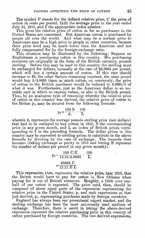
FACTOKS AFFECTING THE PRICE OF COTTOÎT 45

The symbol P stands for the defined relative price, C the price of cotton in cents per pound, 12.21 the average price in the year ended July 31, 1913, and I the appropriate index number.

This gives the relative price of cotton as far as purchasers in the United States are concerned. But American cotton is purchased by people all over the world. And what may be a normal price to Americans may be a high price to people in other countries, because their price level may be much lower than the American and not fully compensated for by the foreign-exchange rates.

This situation may be illustrated by the following: Suppose an Englishman is purchasing cotton in this country. His purchasing resources are originally in the form of the British currency, pounds sterling. Before this may be used in this country the sterling must be exchanged for dollars, normally at the rate of $4.8665 per pound, which will buy a certain amount of cotton. If this rate should increase to $5, the other factors remaining constant, the same pound would buy 5/4.8665 times as much cotton, or, conversely, the price of cotton to the British purchaser would be reduced to 4.8665/5 of what it was. Furthermore, just as the American dollar is an unstable unit in which to express values, so also is the British pound. Thus, by an analogous type of reasoning whereby the relative price of cotton in this country was derived, the relative price of cotton to the Briton Pf, may be secured from the following formula :

100 S 100

wherein £o represents the average pounds sterling price (not dollars) that had to be outlayed to buy cotton in 1913, S the corresponding price in any given month, and L an index of British prices corresponding to I in the preceding formula. The dollar prices in this country may be converted to sterling prices to substitute in the above formula by dividing by the rate of exchange. The formula then becomes (taking exchange as parity in 1913 and letting E represent the number of dollars per pound in any given month) :

100 C/E 100 P*~ 12.21/4.8665 ' L

48665 C "12.21 EL

This expression, then, represents the relative price, base 1913, that the Briton would have to pay for cotton in New Orleans when paying for it out of British resources. Eoughly, a little over one- half of our cotton is exported. The price used, then, should be compjosecl of about equal parts of the expression representing the relative price in the united States, p, and such expressions as that just derived, pf, representing purchases made by foreign countries.

England has always been our preeminent export market, and the sterling exchange has been the most universally used medium of exchange. Therefore, there is merit in letting the above-derived expression represent the relative purchasing price in this country of cotton purchased by foreign countries. The two derived expressions,

46 TECHNICAL BULLETIN 50, U. S. DEPT. OF AGBICULTURE

p and Pf, may be averaged to represent the final price of cotton, p to be used as the dependent variable in these studies. Thus

p=(ppluspf)K = 0.5 p plus 0.5 pf

n ^ /IQQQO C\ 1 n ^ / 48665 C \

0.5 C,^^^^/I , 4.8665\ 10000

/I , 4.8665\ (^jpius-ËTr; "12.21

Anc^ní^ 1 4.8665\ = 409 C(^j plus-g-jj-j

The formula was reduced to the last-shown form because that illustrates the easiest arithmetical way of computing the desired value. In the computations L represents the Statist Index of Whole- sale Prices in England. This index is a continuation of Sauerbeck's. It has been published as a yearly index for the years 1847-1910 and monthly thereafter. It includes 45 commodities, materials, and foods at wholesale. The index is an average of relative prices, each relative being given a weight of 1. The original base was 1867-1877, but has been reworked to a 1913 base, as may be found in European Currency and Finance {S7)^ from which the figures used were taken. Prior to 1910 annual figures were used, as only those are available. Prior to 1912 the sterling exchange rate was talien as par.

The " world relative price of cotton," base 1913, is shown as a decimal (rather than percentage) relative in Table 18. The world price is evidently computed by multiplying the New Orleans price by the product of 409 and the elements inclosed in the brackets in the last-shown formula. This product may be termed a " deflator " ; it is the factor by which it is necessary to multiply the New Orleans price in order to obtain the " world relative price." It is shown in Table 19.

RELATIONSHIP OF FACTORS TO PRICE

The preceding section of this detailed analysis has been devoted to a description of certain factors which presumably influence the price of cotton and methods whereby these factors may be reduced to statistical measurements. This section is concerned with the dis- covery and delineation of any statistical relationships between the world price of cotton and these various factors as so measured.

In this detailed analysis an attempt was made by methods of multiple curvilinear correlation to measure the relation of the monthly world price at New Orleans to the following factors :

TIME FACTORS

Symbol Data

t The crop year, beginning June. The value of t was taken as the last two digits of the calendar year in which the initial month (June) of the crop year occurred,

m The month within any given crop year, to take care of any net seasonal movement not adequately adjusted for in supply-price relationships.

Ï^ACTORS AFFECTING THE PRICE OF COTTON" 47

SUPPLY FACTORS

S The indicated, or actual, supply at the beginning- of the month. These data are found in Table 2.

a The " potential " supply, information on which was available nearest the first of the month, except that from January to May, inclusive, the figure for the preceding December was used. These data are found in Table 20, where data from Table 8 and oflScial forecasts for recent years are brought together.

DEMAND FACTORS—SPECIFIC

u — Accumulated domestic consumption to the first of the month. These data are found in Table 13.

e Accumulated exports to the first of the month. These data are found in Table 12.

DEMAND FACTORS—GENERAL

i Accumulated rates of general price changes, obtainable from data applicable to a period not later than the preceding month. These data are found in Table 14.

o Average price of industrial stocks as a measure of business optimism taken concurrently. These data are found in Table 15.

The price in any given month was related to these factors lagged in such a manner as to reflect the information on them prevailing during the month. For example, in June, 1914, the relative price of cotton (Table 18) was 1.17. The values of the independent factors to which this 1.17 was compared were :

t equals 14. m equals June. s equals 3.059 million bales. a equals 13.5 million bales, u equals 5.24 million bales, e equals 9.28 million bales. i equals —0.1282. o equals $81.

The period covered was June, 1905, to May, 1925, inclusive. The coordinate graph is capable of describing any possible relation-

ship between two real variables, and it is thus adaptable for use in a case, such as the present, where it is almost certain that the relationships will not be of a linear or simple curve nature such as could be adequately described in formulas.

In the case of the supply factor, however, no one curve can completely describe the relation between it and price, because this relation changes continually. It changes from month to month and from year to year. Thus 2,000,000 or 3,000,000 bales is not an exceptionally small supply in June, but it would be disastrously small in Januar}^ after the crop had been harvested and ginned. Owing to this seasonal fluctuation in the supply, it is necessary to have different curves showing its relation to price for different months in the year.

In a similar manner, owing to the increase in population and utilization of cotton, what was a depressingly large supply before the World War is not such a large supply since then, and its effect on price is accordingly different, and it is therefore necessary to have a set of monthly curves after the war different from those before.

If, however, the influence of supply is a systematic thing, there must be some fairly close resemblance between the monthly curves before the war and the monthly curves after the war—perhaps that

48 TECHNICAL BULLETIN 50, U. S. DEPT. OF AGRICULTURE

"^¡^i ACTUAL SUPPLY POTENTIAL syppLV. ACTUAL SUPPLY POTENTIAL SUPMT V

\ 1 ... 1 —. ♦ 03

JANUARY \JANUARY JULY JULY "■

»0.2 ,, 1 \ \\ 1 • 0.1

k,y-/9/5 -t6—/9S*- IS J9IS-I6- I92^2S^\ V V IS-ie-192*^ 2S ^ yl9IS-l6-l»Z -2f

0 —^\— V \\ ,9CS-06 ■■"-^

\ A N s. Vv %\\ \A —^

•0.3 >i^ -—-'--r .^.¿T\ •OA

,30S-0 '--'-f^. ' ■*

♦ OA 1 — «0.3

FEBRIW JTC FEBRUARy AUGUS T AUGUST ._._

V • 0 1

\ \ \ v \ 0 J

\ \ \ \S \ V\ -0.1 -vVi V \^ •^ s^-

•0.2 -\ "* " \ -0.3 \ "■ ^ '- -OA L -, .0,

. ._ ■

•OJ»

♦ 0.S MARO MARC » SEPTEM BER \SEPTEMBER

♦ 0.1 —w \ \ •0.1 vs ^ \ A

0 ■ *J \ -

N, V ■

\ \ •0.1 A s r**- *-«^ \ -0.2 ■\

"- \ -X -0.J \i

'.. '0.1* S , .,. •as . . . , _J_J_ .... .... , , , , •a«. ■ \

— • 0.S

APRl APRl . OCTOB 'Jfí V OBER ■"~

-i9os-oe- ...^ V

— ♦ai Vi r 1

ISI*-IS ^ ,«/5-/«-/ 2V-25 k' ISOS-OS—/t

0 • 1

u ^ P*!«^ \ Ä. -0.1 \^ ==-T - Ny^/S/5- S-/914-2S V •M \ laos-oe -«/♦-,i^

-A/*-/*¿-' •0.* -K- IS-.'e~/92*- -25

\ ♦as

♦OA

\ ^ , \

— ♦ 0.3

MAY NOVEM BER \NOVEMBER

—V— \^ ♦ 0.1 \ \\ ^

0 - ., \ S^ \\ V'- -0.1 S i\ ^A "V" s '»^ \\

». •0.3

\ 'OM

\ 1

,,,, __ ,,,. 1,... • 0.* 1 \

— •e.i -V

JUN JUN DECEMBER V ♦ OS ~'\—i v

V 1 N^ —

0 '• ~\ __ is^^._ \\ \~^

•0.1 AA \\ V.^ ,_ ••■2 \^ \\ _Y_j

•M _^-.. '^ •0.«» -^, -«.8 .... ' , . . . .... _i-<

* - ACTU

SU AL PPLY IN Ml LU ON S OF BALES

POTENT AL

SU 'PLY IN Ml

5

-LIONS OF BALES POTENT

y T AL

Ï—J

FIG. I4.-RELATI0N OF THE ACTUAL SUPPLY AND POTENTIAL SUPPLY TO COTTON PRICES

Actual supply affects prices throughout the year, and potential supply has a diminishing, though little effect on price between January and July, inclusive. Relative price deviations shown, here ahove and below zero represent deviations from the price trend in flg. 19.

FACTOBS AFFECTIÎTG THE PRICE OF COTTON" 49

the whole set of curves representing the postwar period have been moved over to cover a range representing larger supplies. And, indeed, this proves to be the case, as may be observed by inspecting the family of curves representing the relation of (actual) supply to price. Figure 14. The postwar curves (solid lines) in practically all instances have .similar slopes and shapes to those of the pre-war curves (broken lines). But in practically all instances the postwar curves are to the right of the pre-war, representing larger supplies.

If, furthermore, the influence of supply is a systematic thing, then the curves representing the effect on price should move to locations on the graphs representing increasing and then diminishing quantities of supply as the crop year is passed through, corresponding to the market's acceptance and discounting of a seasonally changing supply. And this, too, proves to be the case as inspection of the curves reveals.

This agreement between the quantitative, or mathematical, relationships with what are conceived from a theoretical standpoint to be the true relationships encourages placing confidence in these curves.

The family of curves representing the relation of "potential" supply to price may also be observed in Figure 14. But these curves should exhibit characteristics different in some respects from the " actual " supply curves, reflecting the different conceptions the two represent. In the first place there is no acceptance of a systematic seasonal change in forecast production. For this reason then, the curves should not and do not move into locations representing systematic changes in size of forecast production.

On the other hand, the potential supply in the months of Janu- ary to July is not of much significance nor capable of accurate determination. These curves, then, should demonstrate a diminished importance of potential supply during these months. Or, statistically speaking, a unit change in potential supply should have a reduced effect on price. This type of change is brought about by reducing the slope of the curves. When a curve becomes completely horizontal, as in the case of June, pre-war period, it means that, no matter what the potential supply, there is zero-price effect. With this under- standing, the diminished significance of potential supply in the period, February to July, is well demonstrated by the leveling out of the curves in that period.

In connection with the supply factors it is desirable to consider the curves showing the net seasonal price changes, since the greatest seasonal element is in supply. The curves are observable in Figure 15. They are not of much significance, but may be taken as residual (though systematic) seasonal influences that were not completely absorbed in the shifts of the supply curves. The pre-war and postwar periods in which these seasonal curves were computed coincide with the periods in which supply curves were determined.

Turning to the curves representing the relation of demand factors to price, the factors e and u may be considered. The curves (fig. 16), representing the relation of these two factors to price, are essentially of a similar shape, and they should be so, for one represents the degree of market saturation in this country, the other the same thing in foreign markets.

71431°—28 é

50 TECHNICAL BULLETIN 50, XT. S. DEPT. OE AGRICULTURE

Both curves are of an S type, indicating that these factors are effective in inducing price changes in the range between the leveling out of the curves at their ends. This would suggest that the statisti-

RELATIVE PRICE

tO.2

-0.2

•OA

y ^

^ /50J-/

■Á /

JUNE JULY AUG. SEPT. OCT. NOV DEC. MONTH

JAN. FEa MAR. APR. MAY

FIG. 15.—NET SEASONAL CHANGE IN WORLD RELATIVE PRICE OF COTTON

In addition to the effect of actual and potential supplies on the price of cotton there are other unmeasured factors which produce a seasonal variation, with prices lower than the yearly average during August and September and somewhat higher during December and January. Relative price deviations shown here above and below zero represent deviations from the price trend in fig. 19.

J^ELATIVE PRICE

♦ 0.2

-0.2

-O.-if

\ N/ ■ Exports

Cons jmptlon ^ \ \^

MILLIONS OF BALES

FIG. 16.—RELATION OF ACCUMULATED EXPORTS AND DOMESTIC CONSUMPTION TO THE WORLD PRICE OF COTTON

Both curves indicate that within certain limits (5,000,000 to 7,000,000 bales for exports and 4,500,000 to 6,000,000 bales for domestic consumption) an increase in the quantity of cotton that has already gone into channels of final consumption tends to lower prices, and vice versa. Relative price deviations shown, here above and below zero represent deviations from the price trend in fig. 19.

cal measurement of " saturation " was imperfect, but it in nowise invalidates the curves.

Figure 17 shows the relation between the average price of industrial stocks and the relative price of cotton. Owing to the gradual increase through the period in the average stock price, which was

FACTOES AFFECTING THE PRICE OF COTTON 51

conceived to be depressing, it was necessary to divide the 20-year period into three periods, for each of which a relationship curve was constructed. This situation is similar to that necessitating a division of the period in describing the supply-price relation. An interesting conclusion to be drawn from the industrial-stock-price curves is that low stock prices tend to be associated with low cotton prices, whereas high stock prices fail to be accompanied by materially higher cotton prices, showing no measurable relationship when they are above an average of $100. It is also interesting that in the earliest period the industrial-security prices failed to exhibit any measurable relationship to cotton prices. At that time the security market was apparently not considered a good barometer of business conditions so far as cotton was concerned.

80 90 100 STOCK PRICES, DOLLARS

FIG. I7.-RELATI0N BETWEEN PRICES OF 20 INDUSTRIAL STOCKS AND WORLD PRICE OF COTTON DURING THREE PERIODS

Prior to 1913 prospective business conditions as represented by industrial stock prices had no effect on cotton prices. During the war period a decline in stock prices from $80 to $50 tended to be accompanied by the same reduction in cotton prices, which more recently has accompanied a decline from $100 to $70. High stock prices have failed to be reflected in higher cotton prices. Relative price deviations shown here above and below zero represent deviations from the price trend in fig. 19.

The relation of the accumulated rates of general price change to cotton price is shown in Figure 18. In this it is exhibited that a period of rising general prices heralds increases in the relative price of cotton. The inverse is also true, because the curve has a positive slope throughout its entire length except for large values of the accumulation where the curve levels out.

The remaining factor included in the detailed analysis was a time measurement, taken empirically as the last two digits of the calendar year. This measurement was introduced on the assumption that it was proportional to changes in otherwise unmeasured factors influencing cotton price, such as increasing population, increasing costs of production, and utilization of cotton. The curve showing this relationship or "net trend" in price is given in Figure 19. Its general slope is positive. Its chief pecularity is the dip in it coinci- dent with the commencement of the World War. This is a reflection of the price disturbances.

52 TECHlSriCAL BULLETIN 50, U. S. DEPT. OF AGRICULTURE

PRICE

+ 0.2

^ n .

-0.2 /

y^

^ /

5 -1. 3 -0 5 C ) +0.5 +10 +1.5 +2.0 +2.i ACCUMULATED RATE OF PRICE CHANGE

FIG. 18.—RELATION BETWEEN ACCUMULATED RATES OF GENERAL PRICE CHANGE AND RELATIVE PRICE OF COTTON^

An accumulated advance in the general commodity price level is reflected in an advance in cotton prices, whereas a similar decline in commodity prices is reflected in a greater decrease in cotton prices. Relative price deviations shown here above and helow zero represent deviations from the price trend in fig. 19.

1.4

1.2

1.0

1907 1909 1911 1913 1915 1917 1919 YEAR BEGINNING JUNE

1921 1923 1925 1927

FIG. I9.-THE EFFECT OF CHANGES IN DEMAND ON PRICE (NET PRICE TREND)

These changes were due to the increase in demand and uses for cotton during the past 20 years. Had the production, the general commodity price level, and stock prices remained as in 1906, the increased demand for cotton would have increased its world relative price from about 0.90 in 1906 to 1.50 in 1925. The sharp dip beginning after 1913 shows the falling off of demand with the outbreak of the war.

All of the curves were obtained by methods of repeated simultaneous approximation.^

'^ Technically speaking, the functions in the following equation were determined, wherein P represents the world relative price at New Orleans :

P^'FiíFaít) +Fs(m, t) +F4(S, m, t) 4-F5(a, m, t) +P6(e) +F7(u) -fFgCo) +F9(î)) ' Pi is found in Figure 20, P2 in Figure 19, Fs in Figure 15, B\ in Figure 14, F5 in.

Figure 14, Fe m Figure 16, P7 in Figure 16, Fs in Figure 17, and F9 in Figure 18. The solution for a function, Fi, of the sum of all other functons was suggested and the method worked out by Donald Bruce, of the U. S. Forest Service. See BRUCB^ D,, ON POSSIBLE MODIFICATIONS IN THE EZEKIEL METHOD FOR HANDLING CURVILINEAR MULTIPLE CORRELA- TION. [Unpublished manuscript. Copy on file, Library, U. S. Dept. Agr.]

FACTOES AFFECTIÎÎ^G THE PBICE OF COTTON 53

By securing regression estimates of the dependent, that is, by ascertaining the hypothetical price that would have occurred if the discovered relationships were perfect and all-encompassing, and by comparing the hypothetical prices with the actual, a measure of the reliability of the relationships may be secured. To accomplish this the effects on price of each variable in each month are determined by reading them from the curves and these effects, or functions are then added together. This process gives a hypothetical or " estimated " price, which has a high degree of correlation with the " actual " relative price.

But before this sum (of the readings and constant term) is compared with the actual price it is advisable to ascertain if there is not some systematic relationship between the two, other than the "one- to-one " relationship which a direct comparison would imply. Thus it is easily possible to conceive that if there were a combination of the independent factors which would make for a high price their joint effect on price would be greater than the sum of readings from the curves which typify only the average net relationship through the period. For example, a decrease in actual supply of 10 per cent might mean an increase in price, on the average, of 11 per cent. Similarly, a 10 per cent decrease in potential supply might, on the average, mean an 11 per cent increase in price. But if there should be a 10 per cent decrease in potential supply and actual supply at the same time the joint effect on price might easily be more than 22 per cent, for this would herald a critical situation.

If there is a systematic tendency of this nature it may be easily observed by making a dot chart in which one dimension is the estimated price and the other the actual. If there is a one-to-one relationship the curve drawn to pass through the most dots will be a straight line with a 45° slope. When this test was made, however, it was discovered that the curve drawn to pass through the most dots had a pronounced curvature and was of a nature to verify the sup- position set forth in the preceding paragraph. This curve is shown in Figure 20. It shows that when the estimated price is high it will more closely approximate the actual price if it is made even higher. On the other hand, when it is as low as 0.50 it can go as low as 0.10 while the actual price remains between 0.60 and 0.50.

Since there is this systematic relationship between the estimated price and the actual, it is evidently desirable to employ it in making estimates of the actual price. In short, 1.20 plus the sum of the readings from the relationship graphs should no longer be called an estimated price ; for convenience in reference this quantity may be designated Q. The true estimated price P', should then be secured by reading the height of the curve. Figure 20, at a point above the given value of Q.

Accomplishing this for each month and correlating the "estimated" or hypothetical relative price, P', thus secured, with the actual, relative price, P, gave a correlation coefficient of 0.948, which is unusually high when it is remembered that this analysis covers a period including the panic of 1907, the World War, and the inflation, crisis, and depression following the v/ar.

The fact that the various relationships set forth have consistently held true through a wide range of economic circumstances to a degree

54 TECHNICAL BULLETIN 50, U. S. DEPT. OF AGEICXJLTURE

measured by a correlation of 0.948 is evidence in itself of a measure of stability in them and thus encourages acceptance of them as approximately the true quantitative relations among these factors and price.

On the other hand, there are certain considerations which would tend to modify such a conclusion. No factors on foreign demand other than accumulated exports have been included. No factors on world supplies or production as distinct from those in the United States have been included. And only six of the many statistical series on cotton available in the United States have been included. This forces the conclusion that 90 per cent (K^) of the variability in the relative price of cotton, as measured, is attributable to the six

RELATIVE PRICE

1.80

1.60

1.40

1.20

1.00

0.80

0.60

0.40 .60 .80 1.00

SUM OF READÍNGS 2.00

FIG. 20.—RELATION BETWEEN THE SUM OF READINGS FROM FIGURES 14-19 AND THE WORLD RELATIVE PRICE OF COTTON

Small sums of readings give estimates of relative cotton prices not quite so low, and large sums give estimates of relative prices somewhat higher.

factors (and time measurements) included in the analysis or to factors which are indirectly measured to the degree that they are correlated with those included.

Have such other factors, then, been largely uninfluential in determining price? Such would appear to be the case; but there is no certainty that other factors may not come to be of pronounced significance in the future. This should be remembered in applying the results of this study.

Yet another caution should be observed. The functional relation of the various factors included have been determined from 240 observations by approximation methods. To some degree the correlation between P and P' is due to the pure mathematical probability of fitting these functions to 240 random observations. The degree to which this probability affects the relationship can not be measured without knowing the number of constants necessary to define the

FACTORS AFFECTING THE PRICE OF COTTOK 55

various curves mathematically. If the total number, however, were as great as 120, the correlation would only be reduced to 0.894.^

Of the 90 per cent of price variability attributable to the factors included approximately 26.3 per cent is attributable to the net trend element, 38.7 per cent to the supply elements, and 25 per cent to the demand elements, which verifies the hypothesis that variations in supply factors are of more importance in determining the price than are variations in demand.^

It is of interest to reconvert the actual and estimated relative prices to currency prices and compare the two. The actual New Orleans average monthly spot price in cents per pound is what will be obtained by reversing the deñating process in the case of the actual price, for this is the actual price from which the relative price was obtained. This series may be found in Table 18. It remains to convert the estimated relative price to a doUars-and-cents basis. This is to be accomplished by dividing by the deñator factor. The deflator, or factor by which it is necessary to multiply the currency price to obtain the relative price, was discussed elsewhere, and is shown in Table 19. It was found, however, that when the deflator is relatively small in value better reconversion to currency prices is obtained by making the deflator even smaller. This is a situation analogous to that whereby the estimated relative price, P', was obtained from the quantity Q and is attributable to the fact that the price-level indices from which the deflator was constructed are not only measures of currency value but also, to a degree, of general demand conditions. The curve showing the relation between the value of the deflator and the best value to use in converting the estimated relative price to estimated currency price is given in Figure 21.

Each estimated relative price, P', was divided by the proper value of the deflator, giving a conversion to an estimated currency price of cotton at New Orleans in cents per pound.

A graph (fig. 11) was then constructed showing the actual New Orleans price and this estimated New Orleans price. The agreement between the two is exceptionally close. The correlation coefficient is 0.983. The reason that this coefficient is larger in value than the 0.948 obtained from relative prices is that a considerable portion of the variability in the currency price of cotton is directly due to the variability in the general price level. When this variability is rein- serted in the price by reconverting to currency prices the proportion that the differences between actual and estimated prices is of the total variability in the actual price is reduced, and the correlation coefficient is after all nothing but an inverse measure of this proportion.^^ From another point of view the increased coefficient of cor-

*For theory and method of computing correlation coefflcients adjusted for number of independents see Smith, B. B., Forecasting the Acreage of Cotton (il, p. Jfl, footnote).

^ These percentages were obtained by correlating the readings from function graphs which make up Q' with Q and computing the coefficients of determination (11, p. Iß, footnote). These coefficients were then multiplied by 0.900 (which is R^), which is the proportion of the total squared variability in P attributable to Q through Q's complete determination of P'.

^^ For if sz be the standard deviation of the residuals and Sp the standard deviation of price, then (SZVSP^) is the proportion that the squared variability of the differences is of the squared variability in the price, and the coefficient of correlation is equal to ■^ _,—2/ 2 y ^^ reinserting the price-level influence the standard deviation squared of price was increased 2.96 times as much as was the standard deviation squared of the residuals.


relation may be interpreted to mean that, although absolute accuracy in estimating the price has not been increased, relative accurracy has been increased, owing to the larger base to which errors of estimating are compared.

CONCLUSION

It seems to have been reasonably demonstrated that the price of cotton, to a surprising degree, can be statistically explained as the

VALUE TO USE IN

CONVERSION

0.09

0.08

0.07

0,06

0.05

0.04

0.03

0.02

0.01

.04 .05 .06 VALUE OF DEFLATOR

FIG. 2L—GRAPH FOR ASCERTAINING THE BEST VALUES OF DEFLATOR FOR USE IN CONVERTING ESTIMATED RELATIVE PRICES INTO CENTS-PER-POUND PRICE

When the value of the deflator, or adjustment for converting world relative prices to prices in cents per pound, is below 0.04, a still lower value should be used in the conversion.

reflection of a few selected, fundamental factors, or of others correlated with these selected factors. It is true that not all the variation in the monthly price of cotton during the last 20 years can be adequately allocated to systematic, specific causes, for the correlation between the prices and the selected factors is measurably less than perfect. Nevertheless, the correlation is unusually high for economic or social statistics and lends strength to the belief that cotton prices are definitely responsive to certain groups of influences.

FACTOES AFFECTIÎ^G THE PBICE OF COTTON 57

TABLES

TABLE 2.—Data for forecasting cotton acreage harvested in United States

Index of wholesale prices of

farm products, Decem- ber, preceding year i

Price of cotton preced-

ing year 2

Price of cotton

divided by index of farm- product prices 3

United States cotton acreage har-

vested

Percent- age of increase or decrease

in acreage from pre-

ceding year

Readings from curves <

Calendar Year

of harvest

Relative price Acre- age

change in preceding year

Sum of year

One year pre-

ceding

Two years pre-

ceding

Per cent

reading or fore-

cast of change

1902 81 79 78 80 81 85 86 91

107 97 96

101 103 101 105 146 207 227 242 152 120 145 145 157 152

Cents per pound

8.12 8.29

12.76 7.66

11.88 9.79

10.91 8.72

15.36 15.06 8.87

12.63 12.67 7.48

12.44 18.37 28.98 26.31 34.66 15.12 17.81 25.63 34.99 23.81 20.55

Cents per pound

10.0 10.5 16.4 9.5

14.8 11.5 12.7 9.6

14.5 15.5 9.2

12.5 12.3 7.4

11.8 12.6 14.0 11.6 14.3 9.9

14.8 17.7 24.1 15.2 13.5

Million acres

27.2 27.1 31.2 27.1 31.4 29.7 32 A 30.9 32.4 36.0 34.3 37.1 36.8 31.4 35.0 33.8 36.0 33.6 35.9 30.5 33.0 37.1 41.4 46.1

«47.2

Per cent +1.5 -.4

+15.1 -13.1 +15.7 -5.1 +9.2 -4.5 +4.7

+11.0 -4.9 +8.2 -.9

-14.7 +11.4 -3.4 +6.5 -6.7 +6.8

-15.0 +8.2

+12.4 +11.6 +11.5 +2.2

Per cent

Per cent

Per cent

Per cent

1903 +2 +2 +2 +3 +3 +4 +5 +5 +5 +6 +4 +3 +2 +1

0 -1 -3 -5 -6 -5 -2

0 +1 +2

-8 +6

-12 +4 -8 -2

-12 +3 +6

-14 -2 -3

-23 -4 -2 +2 -5 +2

-10 +4

+12 +13 +5

0

0 0 0

+1 0 0 0 0 0

+1 0 0 0 0 0 0 0 0 0 0 0

+1 +7 +1

+4 +5 -3

+11 -4 +7

0 +7 +2 -1 +7

0 +5

+12 -1 +6 +1 +8 +1

+12 +1 -2 -1 -1

—2 1904 +13 1905 -13 1906 +19

—9 1907 1908 +9

—7 1909 1910... +15

+13 1911 1912 —8 1913-. +9

0 1914 1915. —16 1916 +9

—3 1917 1918 +7

—7 1919 1920.... +5

-15 1921 1922.. +11

+11 +12 +12

1923 1924 1925.... 1926 - +2

11913=100, Bureau of Labor Statistics (35). 2 Price in December for March delivery at New York. 3 Column 3 divided by column 2. 4 See fig. 12. Í Preliminary,


TABLE 3.—Data used m securing supply-price and supply-value curves

Year Supply of cotton 1

Average Decem- ber spot

price New

Orleans

Index of wholesale "all commodity" prices, Decem-

ber 2

Index of wholesale

prices raised to

1.548 power 3

Deflated Decem-

ber price <

Deflated Decem-

ber prie« estimated

from supply 5

Actual Decem-

ber price adjusted to price level of

150 8

Esti- mated

Decem- ber price adjusted to price level of

150 7

1905.

Million bales

12.5 14.6 12.6 14.4 11.4 12.6 17.1 15.5 15.7 17.6 15.5 14.9 14.5 15.9 16.6 18.0 15.1 12.9 12.5 15.1

Cents 11.9 10.5 11.5 8.8

15.0 14.9 9.2

12.8 13.0 7.2

11.9 18.3. 29.1 29.4 39.9 14.6 17.2 25.5 34.9 23.7

87 92 91 93

103 96 94

101 99 97

108 149 182 202 223 179 140 156 151 157

1005 1097 1078 1113 1307 1170 1133 1266 1230 1191 1405 2311 3152 3699 4312 3073 2099 2482 2361 2508

Cents 11.8 9.6

10.7 7.9

11.5 12.7

'. 8.1 10.1 10.6 6.0 8.5 7.9 9.2 7.9 9.3 4.8 8.2

10.3 14.8 9.4

Cents 12.0 9.2

11.8 9.4

14.0 11.8 7.0 8.3 8.1 6.7 8.3 8.9 9.3 8.0 7.4 6.4 8.7

11.4 12.0 8.7

Cents 27.6 22.4 25.0 18.5 26.9 29.7 18.9 23.6 24.8 14.0 19.9 18.5 21.5 18.5 21.7 11.2 19.2 24.1 34.6 22.0

Cents 28.0 21.5 27.6 22.0 32.7 27.6 16.4 19.4 18.9 15.7 19.4 20.8 21.7 18.7 17.3 15.0 20.3 26.6 28.0 20.8

1906 1907 1908 _ 1909 1910 1911 1912 1913 1914 .._ 1915._ 1916 1917 1918._ 1919 1920 . _ 1921 1922 . 1923 _.. 1924

1 Carry over at beginning of crop year and production. 2 Bureau of Labor Statistics, 1913=100. 3 Referred to as the "stepped-up" deflator. * Obtained by dividing column 3 by column 5 and multiplying by 10,000.

889 » From formula 1,000 ^TTTöJ*

1501-848 8 Column 6 multiplied by

' Column 7 multiplied by NOTE.

1,000 150 ^-»^8

1,000 *

Regression equation P= .889 11-«^8 g -i-708. Correlation coefficients (correlating logs) :

Rp.is=0.9555. 'Pi.8=0.911. '■ps.i=0.791.

Normal equations (in terms of coded logs) :

I S P

I 341,143 40,431 59,177

459,422 -31,299

837,829

II 3

cr- _

b= -fl.548 -1.705

Correlation between P and S, after taking I out of P (14, p. 99).

R2 (P-b, I). S: 837829 (1-R2) ■^ 837829-(2) 1.548(459422)*

4-1.5482(341143). 8.38 (.083) ~^ 8.38-3.096(459)*

+2.395(341). = .704

R =.84 Plotting column 2 and 9 gives supply-price curve with prices adjusted to 150 price level (see fig. 4)

and for demand fluctuations correlated with price-level fluctuations. Plotting column 2 and 8 would give scatter diagram for the same curve.

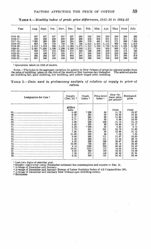
FACTORS AFFECTING THE PRICE OF COTTON- 59

TABLE 4.—Monthly index of grade price différences, 1915-16 to 1924-25

Year Aug. Sept. Oct. Nov. Dec. Jan. Feb. Mar. Apr. May June July

1915-16 327 230

1263 838

1,013 2,025

550 450 263 637

327 230 263 738

1,013 11,650

575 400 288 500

327 230 263 738 988

1,300 575 375 437 450

327 230 288 738

1,125 1,200

625 325 599 450

327 230 288 738

1,200 1,200

575 275 649 380

282 230 364 738

1,375 1,350

550 275 549 380

282 230 376

1,213 1,375 1,275

550 250 524 390

282 230 463

1,213 1,450

850 500 250 549 390

250 211 513

1,113 1,750

850 450 250 524 390

250 211 575 963

1,925 800 450 250 574 390

250 211 600 945

1,925 675 475 250 589 390

250 1916-17... 211 1917-18 1918-19

1888 1,013

1919-20 2,025 1920-21 .__. 575 1921-22 450 1922-23-.. 275 1923-24 674 1924-25 320

1 Quotations taken on 16th of month.

NOTE.—The index is the aggregate variation (in points) in New Orleans of prices for selected grades from the price of middling, taken on the 15th of the month or first business day thereafter. The selected grades are middling fair, good middling, low middUng, and yellow tinged strict middling.

TABLE 5.- -Data used in preliminary analysis of relation of supply to price of cotton

Designation for time i Supply (Dec. 31) 2

Grade index 3

Price-level index *

New Or- leans price per pound «

Estimated price

05.-

Million bales

6.02 6.83

. 6.17 6.77 4.96 5.42 8.24 7.70 7.88

11.69 9.80 8.42 8.22

10.00 9.18

10.87 9.05 7.36 6.43

6 220 282 295 274 229 229

6 230 251 340 328 305 230 326 738

1288 1275 563 275 599

88 92 90 93

103 96 95

101 99 98

111 151 183 201 228 175 139 156 151

Cents n.72 10.50 n.69 9.06

15.10 14.90 9.35

12.70 12.96 7.53

11.97 17.84 30.07 29.14 40.09 14.59 16.85 26.50 34.42

Cents 10.87

06- 10.25 07 - 11.24 08.-- 10.93 09.-- - ._ 18.14 10 15.17 11-- 9.75 12 11.65 13 11.12 14.._ . 7.35 15. .- 10.89 16 -- 20.73 17 28.40 18 26.20 19 ._ 34.50 20-. ... 19.91 21 - 18.08 22. 27.91 23 30.44

1 Last two digits of calendar year. 2 Supply—carry-over—crop (December estimate) less consumption and exports to Dec. 31. 3 Average of December and January. < Average of December and January Bureau of Labor Statistics Index of All Commodities (35). « Average of December and January New Orleans spot middling cotton. 6 Estimates.

60 TECHNICAL BTTLLETIN 50, U. S. DEPT. OF AGEICULTTJRE

TABLE 6.—Oinnings, imports, consumption, exports, cmd indicated supply as of the end of specified months, 1905-06 to 1925-26

[000 omitted]

Year beginning August—

1905 August September- October November. December- January February- March April.. May June July--

1906 August September.. October November.. December. _- January February March _ April May Jime July-

1907 August September. _ October November.. December... January February— March April May June July

1908 August September.- October November. _ December... January February March April May June -- July

Gin- nings

Run- ning bales

477 2,538 3,443 2,232 1,035

485 205

80

408 2,472 4,026 3,122 1,713

700 367 175

200 2,060 3,869 2,214 1,609

640 341 125

402 3,548 4,242 2,817 1,456

390 206

25

Im- ports (32)

600- pound

bales

15

Con- sumption 2

Run- ning bales

275 535 682 688 510 460 410 325 255 230 180

201 280 490 640 790 740 455 555 250 280 210 195

220 200 300 550 440 579 484 442 305 265 180 115

290 200 675 825 880 620 520 360 328 282 210 150

Ex- ports (32)

Run- ning bales

323 604 890

1,000 1,097

650 514 479 551 296 326 177

180 503

1,177 1,267 1,330 1,275 867 771 641 337 183 85

67 380 901

1,319 1,309 1,275 738 436 376 282 266 116

Indi- cated

supply (ad-

justed) 3

Bales i 1,935

4,152 6,152 6,734 6,024 5,386 4,698 3,911 3,070 2,552 2,028 1,701

i, 279 ;,172

4 1,236 4,394 6,921 7,664 6,769 5,522 4,614 3,826 3,154 2,496 2,102 1,867


1909 August September October—. November.- December. January—. February— March April May June July

1910 August September.. October November.. December... January February— March April... May June July__

1911 August September.- October November.. December... January February March. April... May June July-

1912 August September- October November. December.. January February.- March April May June July

Gin- nings '■

Run- ning bales

388 2,942 3,688 1,859

770 260 146 20

353 3,127 3,866 2,794

945 290 170 23

771 4,059 5,141 2,846 1,500

590 420 226

731 3,494 4,644 2,985 1,053

330 200 53

Im- ports

500- pound

bales 9

13 5 9

26 31 16 25 16

7 7

Con- sumption 2

Run- ning bales

350 290 610 820 730 550 380 300 170 140 150 135

75 320 680 780 680 440 380 290 240 190 165 125

100 315 585 800 600 800 550 440 370 278 212 180

110 412 484 449 423 510 448 462 479 482 441 462

Ex- ports (32)

Run- ning bales

114 701

1,289 1,080

705 493 332 444 334 288 311 116

240 1,017 1,417 1,351 1,574 1,414 1,244 1,104 704 370 166 119

202 730

,516 ,735 ,391 901 531 372 535 469 224 141

Indi- cated

supply (ad-

justed) 3

Bales 4 1,484

3,852 5,630 5,597 4,958 4,204 3,673 2,966 2,478 2,056 1,601 1,355

4 1,040 3,513 3,509 6,427 5,423 4,341 3,438 2,865 2,447 2,023 1,776 1,646

4 1,375 4,949 8,111 8,853 8,236 6,573 5,319 4,141 3,146 2,570 2,265 2,026

* 1,777 4,891 7,573 8,410 7,697 6,670 5,936 5,246 4,279 3,367 2,735 2,167

) and preliminary reports for crop of 1 Department of Commerce, Bureau of the Census, Bulletin 156 ( 1924. Ginnings interpolated to end of month when necessary.

2 Data for August, 1905-July, 1912, compiled from New York Cotton Exchange Weekly Market Report. Weekly mill takings converted to a monthly basis. Data for August, 1912-September, 1926, compiled from Department of Commerce, Bureau of the Census, bulletins (17-24). Linters have been excluded wherever possible.

3 Indicated supply figures have been adjusted so that the twelfth-month computation yields the new carry-over.

* Carry-over. Bureau of the Census.

Ginnings from Bulletin 156 (24) of the Department of Commerce and preliminary reports for crop of 1924. Exports and imports compiled from Commerce and Navigation reports (S3, 34). Consumption 1912-13 to 1925-26 from bulletins of Department of Commerce (17-24). Prior to 1912-13 mill takings converted to monthly basis from New York Cotton Exchange Weekly Market Report's report of mill takings. Linters have been excluded wherever possible.


TABLE 6.—Qinnings, imports, consumption, exports, and indicated supply as of the end of speoified months, 1905-06 to 1925-26—Continued

[000 omitted]


1913 August September- October November- December„ January February. _ March April May June , July

1914 August September- October November- December.- January— February. _ March April May June July

1915 August- September.. October.- November. _ December— January- February March _.- April May June July

1916 August September. October... November.. December. January..- February- March April May June July

1917 August September.. October November.. December... January February. _. March April May June July....

Gin- nings

Eun- ning hales

799 3,376 4,655 3,258 1,260

360 190

85

480 5,180 4,167 3,246 1,370 800 440

464 3,136 3,779 2,325

933 230 130

71

851 4,149 3,624 1,728

687 160 100 65

615 2,345 4,135 2,529

721 340 330 143

Im- ports (S2)

500- pound

bales

Con- sump ■ tion

Eun- ning hales

432 442 512 456 456 517 455 493 500 467 446 448

384 415 452 421 451 468 463 525 514 494 515 497

464 499 501 515 555 542 541 614 532 576 671 490

558 528 551 583 537 601 547 604 552 615 574 538

522 585 590 516 524 510 571 544 576 516 541

Ex- ports (32)

Eun- ning bales

257 930

1,518 1,501 1,231 1,052

751 695 398 395 296 118

20 124 493 754

1,172 1,348 1,469 1,148

654 597 310 233

150 491 663 512 547 534 689 426 488 473 499 425

384 509 789 725 755 569 323 279 184 303

438 413 504 409 471 454 352 299 202 280 264 202

Indi- cated

supply (ad-

justed)

Bales * 1,511

4,331 6,948 8,275 7,877 6,685 5,711 4,700 3,859 3,059 2,383 1,833

1,448 5,552 9,771

11,830 11,590 10,578 9,071 7,667 6,530 5,463 4,655

* 3,936

3,804 5,975 8,601 9,921 9,795 8,990 7,996 6,975 6,122 5,106 4,052

* 3,140

3,075 6,212 8,522 8,974 8,424 7,481 6,789 6,027 5,118 4,230 3,481

* 2,720

2,348 3,820 6,928 8,473 8,220 7,622 7,124 6,426 5,711 4,895 4,155

< 3,450


1918 August... September.. October November.. December. January—. February March _._ April May June July

1919 August... September.. October.. November.. December. January... February. March April May June July

1920 August September. October November. December.- January February. . March April May June July

1921 August September. October November. December... January February March April May June July

1922 August- September.. October November-. December—- Janua^y— February. March April May June July ,

Qin- nings

Eun- ning hales 1,038 3,292 3,447 1,794 1,203

500 422 210

143 2,307 3,855 2,539 1,165

587 520 210

352 3,578 3,579 2,632 1,414

830 586 300

2,934 3,226

994 242

75 15 6

806 3,594 3,739 1,181

277 100 25

7

Im- ports

500- pound

bales 8 2 4

28 14 12 10 16 38 39 18 20

15 57 37 54 51

109 130 140 73 16 21 30

16 6

28 52 72

110 69 56 39 25 14 7

Con. sump-

Eun- ning bales 535 490 440 456 473 557 433 433 476 488 474 510

497 491 556 491 512 592 516 576 567 541 555 525

484 458 401 333 295 366 395 438 409 441 462 410

467 485 494 528 511 627 472 520 444 495 509 458

526 494 534 679 629 610 567 624 577 621 542 463

Ex- ports (32)

Eun- ning bales 276 349 367 337 686 658 449 503 411 444 686 527

474 233 351 922 874 922 634 790 540 359 238 208

145 227 582 681 785 600 484 368 315 473 489 695

416 513 866 630 635 459 326 452 587 457 478 364

365 797 856 605 471 355 310 257 168 213 168

Indi- cated

supply (ad-

justed)

Bales 3,692 6,134 8,804 9,840

10,004 9,312 8,867 8,160 7,318 6,432 5,296

4 4,287

3,488 6,092 8,140 9,335 9,181 8,382 7,897 6,893 5,874 6,006 4,250

4 3, 563

3,318 5,249 8,857

10, 508 10, 870 10, 768 10, 506 10,047 9,352 8,458 7,526

< 6, 534

6,145 6,080 9,991 9,884 9,047 8,186 7,462 6,559 5,549 4,614 3,642

* 2, 832

2,922 5,776 8,224 8,085 7,361 6,557 5,788 4,982 4,251 3,662 2,885

< 2,325

* Carry-over. Bureau of the Census.

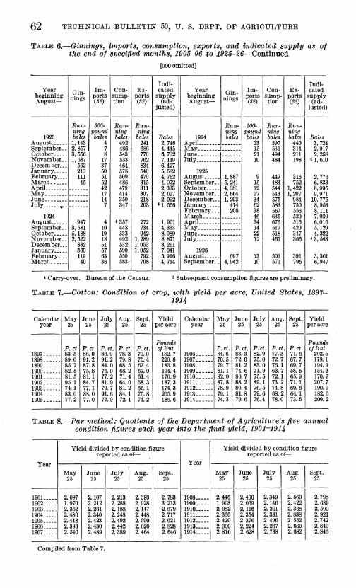
62 TECHNICAL BULLETIN 50, IT. S. DEPT. OF AGRICULTURE

TABLE 6.—Qinnings, imports, consumption, exports, cmd indicateur supply as of the end of specified months, 1905-06 to 1925-26—Continued

[000 omitted]


Gin- nings

Im- ports (32)

Con- sumption

Ex- ports (32)

Indi- cated

supply (ad-

justed)


Gin- nings

Im- ports (32)

Con- sumption

Ex- ports (32)

Indi- cated

supply (ad-

justed)

1923 August September- October November. December.- January February March-_. April May June July ^_

1924 August September-. October November.. December—- January February March

Eun- ning bales 1,143 2,857 3,556 1,687

562 210 111 45

947 3,581 5,188 2,522

882 360 119 40

600- pound

bales 4 7 8

17 37 50 51 52 42 17 14

7

Mun- ning bales

492 486 543 633 464 578 509 486 479 414 350 347

«357 448 533 492 532 590 550

Run- ning

bales 241 686 770 762 834 540 470 315 311 307 218 203

272 734 942

1,289 1,053 1,052

792 708

Bales 2,746 4,445 6,702 7,119 6,427 5,582 4,762 4,072 2,333 2,627 2,092

* 1,556

1,901 4,333 8,089 8,871 8,261 7,041 5,916 4,714

1924 April May June July

1925 August September. October November- December— January February-. March April May June July

1926 August September-

Run- ning bales

1,887 5,241 4,081 2,664 1,293 414

4,942

600- pound bales

23 15 21 10

Run- ning bales

597 531 494 484

449 483 544 543 575 583 567 635 676 517 518 461

501 571

Run- ning bales

440 314 211

316 752

1,422 1,207

984 750 556 520 516 420 347

391 795

Bales 3,724 2,917 2,258

4 1, 610

2,776 6,833 8,995 9,971

10, 775 8,953 8,111 7,039 6,016 5,129 4,322

* 3, 543

3,361 6,947

* Carry-over. Bureau of the Census. « Subsequent consumption figures are preliminary.

TABLE 7.—Cotton: Condition of crop, with yield per aore, United States, 1897^ 19U

Calendar May June July Aug. Sept. Yield Calendar May June July Aug. Sept. Yield year 25 25 25 25 25 per acre year 25 25 25 25 25 per acre

Pounds Pounds P.ct. P.ct. P.ct. P.ct. P.ct. oj lint P.ct. P.ct. P.ct. P.ct. P.ct. of lint

1897 83.5 86.0 86.9 78.3 70.0 182.7 1906 84.6 83.3 82.9 77.3 7L6 202.5 1898 89.0 91.2 9L2 79.8 75.4 220.6 1907 70.5 72.0 75.0 72.7 67.7 179.1 1899 85.7 87.8 84.0 68.5 62.4 183.8 1908 79.7 8L2 83.0 76.1 69.7 194.9 1900 82.5 75.8 76.0 68.2 67.0 194.4 1909 8L1 74.6 7L9 63.7 58.5 154.3 1901 81.5 81.1 77.2 7L4 61.4 170.9 1910 82.0 80.7 75.5 72.1 65.9 170.7 1902 95.1 84.7 8L9 64.0 58.3 187.3 1911 87.8 88.2 89.1 73.2 7L1 207.7 1903 74.1 77.1 79.7 81.2 65.1 174.3 1912 - 78.9 80.4 76.5 74.8 69.6 190.9 1904 83.0 88.0 9L6 84.1 75.8 205.9 1913 79.1 8L8 79.6 68.2 64.1 182.0 1905 77.2 77.0 74.9 72.1 71.2 186.6 1914 74.3 79.6 76.4 78.0 73.5 209.2

TABLE 8.—Par method: Quotients of the Department of Agriculture's five annual condition figures each year into the final yield, 1901^1914

Year

Yield divided by condition figure reported as of—

Year

Yield divided by condition figure reported as of—

May 25

June 25

July 25

Aug. 25

Sept. May 25

June 25

July 25

Aug. 25

Sept. 25

1901 1902 1903 1904 1905 1906 1907

2.097 L970 2.352 2.480 2.418 2.393 2.540

2.107 2. 212 2.261 2.340 2.423 2.430 2.489

2.213 2.288 2.188 2.248 2.492 2.442 2.389

2.393 2.928 2.147 2.448 2.590 2.620 2.464

2.783 3.213 2.679 2.717 2.621 2.828 2.646

1908 1909 1910 1911 1912 1913 1914

2.446 1.903 2.082 2.366 2.420 2.300 2.816

2.400 2.069 2.116 2.354 2 376 2.224 2.628

2.349 2.146 2.261 2.331 2 496 2.287 2.738

2.560 2.422 2.368 2.838 2 552 2.669 2.682

2.798 2.639 2.590 2.921 2.742 2.840 2.846

Compiled from Table 7.


TABLE 9.—Three-pear weiffhted pars, 1904-1915

Three-year weighted moving pars for Three-year weighted moving pars for condition figures as of— condition figures as of—

Par year Par year . May 25 June 25 July 25 Aug. 25 Sept. 25 May 25 June 25 July 25 Aug. 25 Sept. 25

1904 2.186 2.216 2.223 2.430 2.860 1910 2.283 2.252 2.256 2.472 2.688 1905 2.340 2.291 2.238 2.454 2.805 1911 2.101 2.159 2.244 2.423 2.646 1906 2.423 2.366 2.358 2.459 2.661 1912 2.188 2.226 2.273 2.614 2.765 1907 2.418 2.410 2.418 2.577 2.744 1913 2.336 2.317 2.400 2.601 2.765 1908 2.472 2.458 2.426 2.536 2.696 1914 2.349 2.296 2.358 2.668 2.827 1909 2.464 2.433 2.380 2.543 2.758 1915 2.582 2.456 2.554 2.652 2.823

Each par is the weighted average of the quotients in Table 8 for the three years preceding the designated year, with weights of 5, 3, and 2 in receding order. For comparable pars for May of later years see Table 10.

TABLE 10.—Map condition figures, three-year weighted moving pars for May condition figures and estimated (production, 1915^1924

Year

Three-year weighted moving par as of May 25 1

Condition May 25

Estimated production 2 Year

Three-year weighted moving par as of May 25 1

Condition May 25

Estimated production 2

1915 2.578 2.370 2.212 2.181 2.063

Per cent 80.0 11. b 69.5 82.3 75.6

Million hales

13.59 13.86 n.i5 13.88 n.08

1920 -. 2.109 2.457 2.227 2.153 L894

Per cent 62.4 66.0 69.6 7L0 65.5

Million hales

9.80 1916 1921 8.99 1917 1922 1L30 1918. 1923 12.26 1919 1924. _. 10.48

1 For method of computing pars see footnote foF Table 9. 2 Bales of 500 pounds gross weight.

TABLE 11.—United States Department of Agriculture's spring estimate of cotton acreage planted, Decem^her estimate of acreage harvested, and revised acreage harvested, 1900-1924 (25, 27, 29, 30, 31)

(In thousand acres—i. e., 000 omitted)

Year

Spring estimate of

area in cultivation!

December estimate of area picked

Revised (final) esti-

mate of area picked

Year

Spring estimate of

area in cultivation 1

December estimate of area picked

Revised (final) esti-

mate of area picked

1900 25, 558 27,532 27, 878 28,907 31, 730 28,120 28, 686 32,060 32,081 31,918 33,196 35,004 34,097

25,035 26,802 27,114 28,015 30,054 26,117 28,005 31,311 31, 218 30, 780 32,129 34,207 33,581

24,933 26, 774 27,175 27,052 31,215 27,110 31,374 29,660 32,444 30,938 32,403 36,043 34,283

1913 35,622 36,960 31, 535 35,994 34,600 37,073 33,960 35, 504 26, 519 34, 852

■ 38,287 40,403

• 35,676 36, 722 30,957 35,239 33,634 35, 890 33,344 36,383 31,427 33,742 37,420 40,115

37,089 1901 1914 36, 832 1902 1915 31, 412 1903 1916 34,985 1904 1917 33, 841 1905 1918 36,008 1906 . 1919.- __- 33, 566 1907 1920 35, 878 1908 1921 - 30,509 1909.-_ 1922 33,036 1910 1923 .- 37,123 1911 1924 41,360 1912

1 Report issued in June, 1900-11; issued in July, 1912-1924. the United States Department of Agriculture.

Estimates of the crop-reporting board of

64 TECHÍsTICAL BULLETIN 50, U. S. DEPT. OF AGRICULTURE

TABLE 12.—Production of cotton in the united States, estimated from reported condition, pars, and acreage compared with production estimated 'by " regression " method, 1904-1915

[In thousand bales—i. e., 000 omitted]

Year and month of estimate

1904 May June July.. August September.

1905 May June July .. August September.

1906 May June July August September.


Production,! estimated by the use of—

Pars

12,044 12, 945 13, 517 13, 565 14,391

10,627 10,378 10, 963 10,409 11, 749

12,302 11, 828 12,477 11,407 11,434

11,434 11.638 12,666 12, 566 12,460

Regres- sion

equation

12.546 12,612 14,139 13,475 13,940

10,648 10, 530 10,118 10,883 11,707

11,402 11,642 11, 522 11, 582 12,003

11,603 11,134 11, 536 12,542 12, 811


1908 May June __- July August September..

1909 May JuJne July August September..

1910 May June July August September..

1911 May June July August-


Pars

13,223 13,395 13, 514 12, 953 12,612

13,344 12,119 11,426 10,817 10,773

12,460 12,621 11,829 12,378 12,302

13,489 13, 945 14,642 12, 988

September. 13,777

sion equa-

12,416 12,349 12,886 12,819 13,155

12,420 12,487 11,018 11,619 11,352

13,056 13,056 12, 014 12, 917 12,987

14,278 14,646 15,085 13, 692 14, 573


1912 May June July.. August September.

1913 May June....... July August September.


1915 May June __ July August September.


Pars

12,304 12, 766 12,403 13,948 13, 727

13, 770 14,124 14,287 13,220 13, 208

13,495 14,131 13, 929 16,091 16,066

13, 627 12, 995 12, 704 12,107 11,324

Regres- sion

equation

13,125 12,983 12, 626 13, 553 13, 910

13,712 13,638 13, 712 14,457 13, 563

13, 763 14,305 13, 531 15,001 15,774

12,205 12,403 11,413 11,941 11, 545

! Bales of 500 pounds gross weight.

TABLE 13.—Correlation coefficients and regression coefficients of final yield on the several condition figures, product moments, standard deviations, and means used in writing the various regression equations, 1897 to 1913

Statistical unit

Cotton condition figures as of—

May 25 June 25 July 25 Aug. 25 Sept. 25 Yield

Correlation coefficient: Yield, with condition.. _

Regression coefficient: Yield, on condition Means Correlation coefficient: Condition and

yield with time (1905=0) Regression coefficient: Condition and

yield, on time Product moment: Yield, with condition.. Product moment: Time, with condition

and yield Squared standard deviations

0.42 L21

82.24

-. 38235 36.88

-9.18 30.47

0.63 L93

8L82

-.33088 5L76

-7.94 26.82

0.76 2.06

8L12

-.330

-.39216 69.82

0.51 L46

73.24

-.187

-. 21078

-5.06 30.65

0.76 2.34

67.35

-.009

6L82

-.24 26.35

187. 65

-.172

-.55392

-13.29 248. 24

FACTORS AFFECTIiSTG THE PRICE OF COTTON 65

TABLE 14.—Three-year weigJiteH average annual cotton exports from the üniteä States for period ending last dap of specified month, January, 1902-^uly, 1926^

[In thousand bales- tted]

Year Jan. Feb. Mar. Apr. May June July Aug. Sept. Oct. Nov. Dec.

1902, 1903. 1904 1905 1906 1907 1908, 1909 1910 1911 1912. 1913. 1914 1915. 1916. 1917. Î918. 1919. 1920. 1921. 1922. 1923. 1924. 1925. 1926.

6,711 6,803 6,860 6,735 7,308 7,733 8,060 8,180 8,093 7,854 8,386 9,316 9,236 7,946 7,375 6,871 6,609 4,709 6,501 6,768 6,218 6,045 5,703 6,376 7,255

6,725 6,885 6,760 6,708 7,267 7,931 8,104 8,196 7,370 7,664 8,474 9,188 9,223 8,229 7,244 6,598 5,358 4,693 5, 628 6,768 6,131 6,982 6,738 6,577 7,257

6,694 6,962 6,604 6,830 7,189 8,069 7,980 8,207 7,286 7,639 8,792 9,023 9,304 8,406 7,084 6,398 6.179 4,772 6,837 5,684 6,104 5,851 6,716 6,747 7,282

6,671 6,890 6,557 6,961 7,252 8,178 7,866 8,178 7,198 7,579 8,972 9,058 9,276 8,460 7,050 6,247 5,064 4,820 6,967 6,652 6,196 6,723 6,697 6,761 7,369

6,635 6,863 6,472 7,171 7,211 8,196 7,783 8,260 7,156 7,573 8, 974 9,130 9,280 8,558 7,034 6,166 4,977 4,862 5,970 6,716 6,207 6,591 6,678 6,760 7,454

6,607 6,833 6,461 7,359 7, 228 8,137 7,740 8,261 7,192 7,509 8.939 9,131 9,335 8,598 7,147 6,088 4,952 6,030 6,880 6,792 6,188 6,506 5,599 6,696 7,621

6,571 6,789 6,436 7,467 7,228 8,092 7,698 8,280 7,186 7,483 8,937 9.146 9,339 8,653 7,273 6,083 4,913 5,142 6,808 6,954 6,124 6,416 6,512 6,663 7,610

6,576 6,738 6,437 7,575 7,236 8,036 7,690 8,260 7,256 7,507 8,943 9,161 9,229 8,658 7,382 6,206 4,895 6,204 6,670 6,030 6,066 6,412 6,489

6,676 6,603 7,548 7,213 7,909 7,775 8,339 7,355 7,660 8,883 9,226 8,829 8,640 7,340 6,237 4,837 6,108 5,620 6,149 6,077 5,686 6,580 6,777

6,679 6,787 6,651 7,441 7,271 7,794 7, 910 8,413 7,416 7,747 8,981 9,292 8,337 8,418 7,248 6,166 4,708 6,002 5,703 6,357 6,174 6,607 6,643 7,063

6, 754 6,935 6,736 7,414 7,342 7,864 7,984 8,302 7,386 7,816 9,245 9,327 7,969 8,025 7,133 6,024 4,620 5,209 5,744 6,376 6,223 5,618 5,924 7,469

6,767 6,945 6,746 7,392 7,440 7,905 8,149 7,946 7,508 7,948 9,348 9,235 7,856 7,663 7,038 6,819 4,634 6,330 5,809 6,332 6,145 5,694 6,097 7,239

1 In thousand running bales, Unters excluded where possible, i. e., since July 1, 1914. The average for any given month was computed from the export data in Table 6 by summing the 12 months' figures ending with the last day of the specified month and weighting it 6; summing the corresponding 12 months in the year preceding and weighting 3; and summing the corresponding 12 months two years preceding and weight- mg 2. The aggregate of the 36 months thus weighted was divided by the sum of the weights, i. e., 10.

TABLE 15.—Three-year weighted average annual consumption of cotton in the united States for period ending lact day of specified month, 1908-1926

[In thousand bales—i. e., 000 omitted]

Years

1908-09. 1909-10. 1910-11. 1911-12. 1912-13. 1913-14. 1914-15. 1916-16. 1916-17. 1917-18. 1918-19. 1919-20. 1920-21. 1921-22. 1922-23. 1923-24. 1924-26. 1925-26.

Sept.

4,534 4.945 4,642 4,588 4,862 6,235 6,496 5,649 6,100 6,506 6,592 6,172 6,204 6.508 6,734 6,086 6,937 6,136

4,605 5,007 4,742 4,668 4,797 5,200 6,454 5,661 6,128 6,548 6,539 6,193 6,133 6,532 5, 751 6,121 5,942 6,140

Nov.

4,707 5,069 4,776 4,565 4,620 5,102 6,369 6,699 6,183 6,590 6,488 6,172 6,038 5,689 6,804 6,152 6,918 6,144

Dec.

4, 843 6,056 4,794 4,480 4,497 5,049 6,341 5,756 6,204 6,595 6,456 6,174 6,932 6,640 5.834 6,168 5, 936 6,173

Jan.

4,861 5,011 4,726 4,613 4,438 6,038 6,260 5,780 6,246 6,589 6,462 6,186 5,836 6,659 5,878 6,209 6.949 6,167

Feb.

4,887 4,948 4,691 4,670 4,438 6,046 6,246 6,823 6,274 6,588 6,413 6,197 5,785 6,678 6,925 6,224 6,971 6,176

Mar.

4,841 4,870 4,652 4,730 4.490 5,097 5,276 6,883 6,302 6,587 6,332 6,221 5,732 6,706 5,974 6,202 5,999 6,204

Apr.

4, 855 4,810 4,645 4,784 4, 600 6,166 5,311 5, 900 6,320 6,592 6,300 6,2^4 5,666 6,694 6,019 6,200 6,055 6,209

May

4,863 4, 740 4,630 4,815 4,738 5,237 5,361 6,946 6, 370 6,601 6,252 6,237 5,614 5,702 6,078 6,145 6,078 6,196

4,865 4,714 4,626 4,831 4,870 6,318 6,442 5,996 6,402 6,584 6.214 6,253 5,584 5,714 6,090 6,069 6.098 6,213

July

4,861 4,700 4,623 4,852 5,025 5,407 5,519 6,004 6,434 6,598 6,209 6,252 6,525 5,706 6,084 6,022 6,133 6,219

Aug.

4,916 4,600 4,563 4,809 5,192 5,481 5, 609 6,066 6,484 6, 604 6,182 6,227 5, 505 5,728 6,082 5,956 6,132

NOTE.—In thousand running bales. The average for any given month was computed from the consumption data in Table 6 by summing the 12 months' figures ending v/ith the last day of specified month and weighting 6; summing the corresponding 12 months in the year preceding and weighting 3; and summing the corresponding 12 months two years preceding and weighting 2. The aggregate of the 36 months thus weighted was divided by the sum of the weights, i. e., 10.

71431°—28 5

66 TECHNICAL BULLETIlSr 50, U. S. DEPT. OF AGRICULTUKE

TABLE 16.—Rate of wholesale price change in United States, March, 1900-Bep- tember, 1926, and two-year weighted accumulation thereof, February, 1902- Septemher, 1926

Month

Rate of change i

Weighted accumulation of changes 2

1900

Rate of Weighted accumulation of changes 2

1901

Rate of change ^

Weighted accumulation of changes 2

1902

Rate of change 1

Weighted accumulation of

1903

January February. _ March April May June July August September. October November. December..

0 0

-0. 01220

-. 01250 0 0 -. 01250 0 0

-0. 01266 -. 01266 -. 01282 0 0 0 0 +. 01282 +. 03797 +. 01235 0 +. 03704

+0. 01205 -. 02439 -. 01235 +.01235 0 +.02469 +.04762 -. 01176 -. 01205 -f. 09524 +. 03297 -. 03448

+0.1112 +. 0664 +.1038 -f. 1158 +. 1740 -f. 3012 -f. 2779 +.2210 +. 4552 +.5560 4-. 4424

+0. 03409 +.01111 -. 03371 -. 03448 -, 02326 -. 01176 -. 01176 -. 01190 +. 01190 0 -. 01190 0

+0. 4776 +. 5082 +. 4090 +.2458 +.1769 +. 1432 +. 0521 +. 0211 +. 0544 -. 0014 -. 0240 -. 0138

1904 1905 1906 1907

January. _. February. March April May June July August September October. _- November December.

January February.. March April May June July August September October November. December.

January..- February.. March April May June July August September. October November. December.

+0. 02381 +. 03488 +. 01149 ~. 02299 -. 03529 -. 01190 0 +. 01190 +. 02353 +. 01163 +. 01163 +. 02299

-0. 0020 +. 1040 -f. 1572 +. 0403 -. 0605 -. 0776 -.1214 -.0847 +. 0050 +. 0080 +. 0362 +. 1125

0 -0. 01149 -. 01149 0 -. 01149 -. 02353 0

-f. 01176 0 0 +. 01176 +. 01176

+0.1125 +.0860 +. 0506 +. 0622 +. 0436 -. 0307 -. 0309 +.0083 +.0007 -. 0035 +.0279 +.0556

+0. 02299 0 -. 01149 +. 01149 +. 01136 0 -. 02273 0 +. 02273 +. 02273 +. 03333 +. 02198

+0.1127 +. 1048 +. 0665 +. 0933 +. 1274 +. 1274 +. 0514 +. 0396 +. 0963 +.1491 +.2301 +.2851

+0. 01087 +. 01087 0 0 +. 02151 +. 02128 +.01053 0 0 +.01053 -.02083 -.05376

+0. 3026 +. 3164 +. 3132 +.2980 +.3328 +. 3825 +.3954 +.3618 +. 3398 +. 3492 +. 2641 +.0987

1908 1909

-0. 04396 -. 03371 0 +. 01124 0 +. 01124 +. 01111 0 +.01111 +. 01099 +. 01099 +. 02174

-0. 0408 -.1494 -. 1496 -. 1192 -.1269 -.1010 -. 0712 -. 0748 -. 0530 -. 0348 -.0092 +. 0448

+0. 01075 0 +. 01075 +. 02128 +. 03158 +. 02062 0 +. 01031 +. 02041 +. 03030 +. 02970 +. 01961

+0. 0664 +. 0701 +. 0949 +.1446 +.2362 +.2837 +.2696 +. 3010 +.3482 +.4184 +.4981 +. 5364

0 -0. +. 02941 +. 02857 -. 01905 -. 02913 -. 00980 0 -. 01961 -. 05000 -. 05155 -. 01053

+0. 5192 +. 4767 +.5167 +.5610 +.4859 +.3599 +. 2961 +. 2782 +. 1911 +.0271 -. 1284 -. 1810

0 -0.1913 -0. 04211 -.3008 -. 02174 -.3725 -. 01075 -.4080 -. 03297 -. 4790 -.01111 -. 5116 +. 02222 -.4485 +. 04348 -.2940 +. 03191 -.2013 +.01053 -. 1768 0 -.1493 -. 01053 -.1737

1912 1913 1914

0 +0. 02105 +. 02083 +. 04124 +. 03000 -. 01000 -. 01010 +. 01010 +. 02000 +. 00990 0 0

-0.1706 -. 0771 -.0078 +. 1052 +.2123 +.2022 +. 1742 +.2119 +. 2754 +.3007 +. 3082 +.3051

-0. 00990 -.01000 0 0 -.01000 -. 01010 +.01010 +.01000 +. 02000 +. 00980 -. 01980 -.02000

+0. 2577 +. 2213 --. 2148 --. 1970 ". 1499 --. 1092 —. 1148 --. 1133 --. 1526 —.1615 —.0916 —. 0282

-0. 02020 0 0 -. 01020 -. 01020 -. 01031 0 +. 04124 +. 04950 -. 03922 -. 05155 0

-0. 0426 -. 0531 -. 0600 -. 0975 -.1282 -.1556 -.1488 -.0288 +. 1034 +.0022 -.1357 -.1453

+0. 01031 +. 02041 +. 01010 0 +. 01010 0 0 +. 01000 0

+. 02000 +. 03922 +. 05769

-0. 0980 -. 0268 -.0095 +.0035 +. 0371 +. 0241 +.0372 +.0638 +. 0474 +. 1172 +. 2217 +. 3658

1 The rate of change for any given month is the Bureau of Labor All Commodity Index (Table 17) for the given month less the index for the second preceding month divided by the index for the first preceding month.

2 The weighted accumulation of change for any given month is computed by combining the rate of change for that month with the rates of change for the 23 preceding months in the following manner: The average rate of change for the given month and the 2 immediately preceding months is weighted 8; the average of the first 3 preceding these is weighted 7; of the next 3, 6; and so on with diminishing weights for every 3 months' grx)up until the average of the first 3 months included is weighted 1. —


TABLE 16.—Bate of wholesale price change in United States, March, 1900-Sep- temher, 1926, and two-year weighted accumulation thereof, Fe'bruary, 1902- Septemher, 1926—Continued

Month

Rate of change


1916

Rate of change

Weighted accumulation of changes

1917

Rate of change


1918

Rate of change


1919

January. __ February- March April May June July August September October. __ November. December.

+0.08333 +. 06195 +. 05217 -f. 05042 +. 02479 -f. 01639 +. 00813 +. 02439 +. 05556 +. 07692 +.11765 +. 08904

-f 0. 6011 +. 7466 -f. 8501 -f. 9631 -f. 9888 -f. 9795 +. 9596 -f. 9725

H-1. 0588 +1. 2196 +1.4868 H-1. 6603

+0. 04698 +. 05229 +. 05732 -f. 09877 +. 12139 +. 06557 -f. 02703 -f. 02128 -. 00529 -. 03209 -. 02186 -.00546

-f 1. 7026 -f 1. 7391 +1. 7984 +1. 9666 +2.1767 +2. 2422 +2.1861 4-2. 0923 +1. 9469 -f 1. 7242 +1. 5115 -f-1. 3675

+0. 00549 +. 02174 -f. 01613 +. 02139 -f. 01579 +. 00526 +. 03141 -f. 04592 +. 04000 +. 00980 -. 00495 0

-f 1. 2623 -f 1.1863 +1.1209 -f 1. 0840 +1. 0056 -f. 9232 +. 9228 +. 9277 +. 9416 +. 8758 +. 7379 -I-.6504

-0. -. 04523 -. 01554 +. 03061 +. 03015 +. 01980 +. 04926 -f. 06132

-. 02381 +. 03318 +. 05530

+Ö. 5280 -f. 3234 +. 2242 +. 2585 +.2875 +. 3067 +. 4135 +. 5560 +. 5130 -f. 4176 +. 4718 +. 6022

1920 1922 1923

January... February- March April May June July August September October... November. December.

+0.07175 +. 03863 +. 00431 -f. 05556 +. 05306 -. 00810 -. 02469 -. 04979 -.06494 -. 08850 -.14218 -. 00510

+0. 7589 +. 8092 +. 7834 +. 8747 +.9579 +. 9031 -f. 7690 +. 5655 +.3635 +.0780 -.3400 -.3474

-0.14525 -.11176 -. 09375 -. 07742 -. 06757 -. 04138 -. 02817 0 0 0 0 -. 01418

-0. 7516 -1.0427 -1.2848 -1. 4662 -1. 6173 -1.6937 -1. 7078 -1.6461 -1. 6918 -1. 5050 -1. 4228 -1.4094

-0. 02143 -f. 00725 +. 02837 +. 01408 +. 04196 +. 04730 -f. 04667 +. 03226 -. 01290 -. 00654 +. 01948 +. 01282

-1. 3879 -1.2751 -1.1251 -.9776 -.7620 -. 5695 -.3213 -.1278 -.1144 -. 0319 +.1002 +.1649

0 +0. 00641 +. 01911 +. 01258 -. 01887 -. 03846 -. 03268 -. 01987 +. 02000 +. 01948 -. 01307 -. 01316

+0. 2376 +. 2808 +. 3564 +.4141 +. 3505 +. 2349 +.1421 +. 0595 +. 0989 +.1466 +. 0888 +. 0331

1924 1925 1926

January.— February.. March April May June July August September October November. December.

-0.00662 +. 00662 -.00658 —. 02667 -. 02027 -. 02041 0 +. 03401 -f. 01333 +. 01342 +. 02632 +.

-0.0048 +.0038 -.0347 -.1215 -. 1939 -. 2576 -.2597 -.1597 -.1178 -.0681 +.0034 +.0950

+0. 04459 +.02500 +. 00621 -. 03106 -. 03846 +. 00645 +. 02986 +.01876 -.01433 -.01713 +.00063 -.00951

+0.2208 +.2870 +.3014 +.2105 +. 1014 +. 1208 +. 2068 +. 2568 +. 2058 +. 1458 +. 1344 +.1077

-0. 01088 -. 00769 -. 02903 -. 02574 +. 00132 -. 00791 -.00656 -. 02057 -.00134

+.0765 +.0385 -. 0416 —. 1109 -.1202 -.1364 -.1549 -.2297 -.2326

68 TECHNICAL BULLETIN 50, U. S. DEPT. OF AGEICULTUKE

TABLE 17.—Prices of 20 industrial stocks (6, p. 302; 7, v. 6, p. 162; v. 7, p. 1^8; V. 8, p. 245; 9, p. 166-167)

Year Jan. Feb. Mar. Apr. May June July Aug. Sept. Oct. Nov. Dec.

1899 Dolls.

62.7 65.7 67.6 63.9 65.3 48.8 70.1 98.7 93.6 62.7 85.6 94.3 83.3 81.3 85.1 80.7 56.6 94.7 97.2 76.6 81.7

104.6 75.1 80.9 97.9 97.4

122.2 156.6

Dolls. 64.8 65.9 68.9 65.1 66.6 47.9 73.6 97.8 91.6 60.4 83.3 88.2 85.2 80.9 81.2 82.3 56.0 93.6 91.0 80.0 82.4 94.5 75.5 84.0

101.8 98.8

121.1 159.2

Dolls. 70.3 63.6 68.6 66.2 64.5 47.8 78.0 95.0 82.8 65.5 83.9 92.1 83.2 85.3 80.0 82.3 58.3 93.3 94.6 78.0 86.6 99.5 75.4 87.3

104.3 96.3

120.9 146.4

Dolls. 75.0 63.4 73.4 67.2 62.7 49.3 80.0 93.5 83.1 68.7 85.9 89.4 82.5 89.8 80.8 79.8 66.4 89.8 93.9 77.6 91.2

100.9 76.7 91.7

101.5 91.7

119.8 140.5

Dolls. 71.8 59.0 71.7 65.9 62.2 48.1 74.7 90.1 81.2 72.5 90.3 87.2 84.5 89.1 79.2 80.5 66.0 90.2 93.4 81.0

100.4 91.4 77.2 93.6 96.2 90.5

126.1 140.2

Dolls. 70.8 56.6 77.2 65.0 58.3 48.8 75.2 91.1 78.9 73.1 92.1 83.8 86.5 89.7 74.7 80.6 68.4 90.6 97.0 80.4

105.4 91.4 69.1 93.4 93.7 92.6

128.8 149.2

Dolls. 72.2 57.3 73.3 64.8 54.0 51.2 79.6 88.8 80.7 76.6 94.8 77.6 85.9 89.9 77.2 76.6 71.9 88.5 92.9 81.8

110.0 90.6 68.5 95.2 89.3 98.3

133.6 156.6

Dolls. 75.0 58.0 71.5 66.1 50.7 53.7 81.7 93.9 74.1 83.0 97.8 78.8 82.2 91.0 80.0

Dolls. 75.0 65.8 69.8 66.0 49.0 56.3 80.3 94.7 70.6 80.9 98.0 79.1 76.6 92.3 81.9

Dolls. 73.0 57.7 64.8 65.2 44.9 61.1 82.3 94.8 62.6 81.6 98.1 83.0 76.8 92.3 79.3

Dolls. 74.5 64.2 65.5 63.2 43.9 68.1 85.4 93.9 55.8 85.7 98.2 84.2 79.8 90.8 77.2

Dolls. 67 0

1900 67.5 1901 63.2 1902 62.0 1903 46.9 1904 69 5 1905 93.1 1906 94.4 1907 59.3 1908 85.6 1909 98.0 1910 81.0 1911 80.9 1912 88.0 1913 77.1 1914 75.2 1915 . 79.2

91.0 88.6 82.0

102.6 85.4 66.8 98.3 90.8

103.3 139.6 163.2

85.5 97.4 83.6 82.5

107.5 87.0 70.2 99.8 90.3

102.8 144.0 160.1

92.4 102.1 79.0 86.2

114.1 84.9 71.3

100.4 87.7

102.0 149.9

94.4 107.9 71.4 84.0

110.8 78.4 76.0 95.8 91.0

108.2 153.9

97.0 1916 98.5 1917 70.2 1918 82.5 1919 105.7 1920 72.0 1921 79.9 1922 97.6 1923 94.1 1924 114.2 1925 154.2 1926

The original source is the Wall Street Journal.

TABLE 18.—World relative price of cotton at New Orleans and Mslc data from which computed, 1900-1926

Year beginning Aug-

ust—

Aver- age

price per

pound at New

Or- leans

Bu- reau of Labor Index of All Com- modi-

ties

Sterling ex-

change!

British price level 2

World price


ust—

Aver- age

price per

pound at New

Or- leans

Bu- reau of Labor Index of All Com- modi- ties

Sterling ex-

change!

British price level 2

World price

1900 August September.. October November.. December... January February. __ March April May June July _

1901 August September-. October November. - December- January February. __ March April May-- - June July

Cents

10.39 9.57 9.48 9.50 9.52 9.20 8.49 8.15 7.69 8.05 8.33

8.28 8.15 7.99 7.32 7.93 7.88 8.08 8.54 9.13 9.39 9.15 8.94

80 80 79 80 79 79 78 78 78 78 78 78

79 81 80 81 83 82 81 81 82 84 84 85

Dolls. 88 88 88 88 88 82 82 82 82 82 82 82

82 82 82 82 82 81 81 81 81 81 81 81

'Í."OÍ40 .9402 .9252 .9333 .9680 .9414 .8688 .8340 .7869 .8238 .8524

.8419

.8183

.8071

.7350

.7865

.7912

.8162

.8627

.9167

.9313

.9075

.8816

1902 August September.- October November.- Decembe^.„ January February. _. March April May_- _ June July

1903 August September. _ October November _ _ December-.- January February.— March April- May-- June July

Cents 8.43 8.43 8.22 7.82 8.14 8.66 9.36 9.73

10.05 n.i4 12.71 13.02

12.70 10.72 9.66

10.72 12.52 14.06 14.38 15.07 14.45 13.41 n.38 10.86

83 84 91 87 88 90 89 87 86 85 85 84

84 85 84 84 84 86 87 87 85 84 84 84

Dolls. 81 81 81 81 81 81 81 81 81 81 81 81

81 81 81 81 81 82 82 82 82 82 82 82

0. 8413 .8361 .7847 .7625 .7893 .8300 .9031 .9488 .9857

1.0985 1. 2533 1. 2913

1. 2596 L 0571 .9581

1.0632 1. 2417 1. 3703 1. 3933 1.4601 1. 4161 1. 3218 1.1217 1.0705

1 sterling exchange taken at parity, $4.8665, prior to January, 1912. 2 British price level is Statist Index Number (continuation of Sauerbecks) (Î). Prior to January, 1910,

only annual indices were available. 3 Market closed.

FACTOES AFFECTIKG THE PRICE OF COTTON 69

TABLE 18.—World relative price of cotton at New Orleans and haste data from which computed^ 1900-1926—Continued


ust—

Aver- age

price per

pound at New

Or- leans

1904 August September.. October November-. December__. January February. _. March April... May June. July..-

1905 August September. October November. December.. January February. _ March April. _ May June July

1906 August September. October November. December.. January February. _ March April. May June _ July

1907 August September. October November. December. _ January February.. March April May June July

1908 August September. October November. December.. January February.. March April May June July

Cents 10.59 10.54 9.80 9.50 7.48 6.83 7.45 7.45 7.39 7.90 8.87

10.61

10.48 10.26 10.16 11.28 11.88 11.56 10.67 10.84 11.28 11.33 10.99 10.96

9.24 10.76 10.39 10.53 10.46 10.49 10.83 10.79 11.85 12.81 12.89

13.13 12.41 11.19 10.84 11.54 11.84 11.63 10.93 10.20 10.86 11.59 10.81

9.92 9.11 8.92 8.97 8.78 9.34 9.42 9.39

10.03 10.59 11.04 12.13

Bu- reau of Labor Index of All Com- modi- ties

Sterling ex-

change

85

87

British price level

Dolls.

World price

1.0378 1.0272 .9551 .9205 . 7208 .6495 .7084 .7127 .7027 .7600 .8533 1.0207

1.0026 .9870 .9720 1.0792 1.1297 1.0567 .9810 .9966 1.0311 1. 0357 1.0046 1.0140

.9132

.8446

.9726

.9341

.9415

.9203

.9178

.9528

.9440 1. 0314 1.1092 1.1161

1.1369 1.0746 .9639 .9484 1.0209 1.1075 1.0936 1.0224 .9541 1.0158 1.0780 1.0054

.9227

.8429

.8253

.8254

.8568

.8499

.9033

.9442

.9843 1.0815


ust—

1909 August September. _ October November _ _ December..- January February. _- March April May.. June July

1910 August September.. October. November.. December. __ January February... March April May June .- July-..

1911 August September.. October November.. December... January February March April May June July...

1912 August September.. October November.. December.. _ January February March April May June July

1913 August September. _ October November.. December... January, February.. _ March April May. __ June July

Aver- Bu- age reau of

price per

Labor Index Sterling British

pound at New

of All Com-

exchange

price level

Or- modi- leans ties

Cents Dolls. 12.28 98 87 12.65 99 87 13.48 101 87 14.40 102 87 14.96 103 87 15.23 102 91 14.88 102 92 14.74 105 93 14.89 105 92 14.64 103 92 14.85 102 90 14.93 102 92

14.92 102 92 13.49 100 91 14.21 97 91 14.50 95 91 14.85 96 91 14.95 95 92 14.62 92 92 14.54 93 93 14.70 91 94 15.48 90 94 15.26 90 94 14.30 92 93

11.96 94 93 11.29 95 94 9.61 95 95 9.35 95 95 9.17 94 95 9.53 95 4. 8748 96

10.31 96 4. 8774 97 10.65 97 4. 8758 99 11.61 100 4.8744 100 11.72 100 4. 8730 100 12.07 99 4. 8760 100 12.93 99 4. 8790 1C2

12.07 100 4. 8755 101 11.37 101 4. 8641 102 10.95 101 4. 8615 101 12.15 101 4. 8579 100 12.81 101 4. 8563 101 12.58 100 4. 8743 101 12.51 100 4. 8813 101 12.45 100 4. 8820 102 12.44 100 4. 8724 101 12.29 99 4.8675 101 12.44 99 4. 8723 99 12.34 100 4.8724 99

12.02 100 4. 8663 100 13.11 102 4. 8596 101 13.73 101 4. 8608 99 13.26 100 4. 8576 98 12.98 99 4. 8595 99 12.93 98 4. 8628 98 12.90 99 4. 8576 98 12.95 98 4. 8623 97 13.11 98 4. 8699 97 13.36 97 4. 8816 97 13.79 97 4.8844 95 13.34 97 4.9013 97

World price

1.0894 1.1179 1.1794 1. 2540 1. 2972 1. 2950 1.2580 1. 2219 1. 2418 1. 2322 1. 2700 1. 2622

1. 2613 1.1581 1. 2380 1. 2763 1. 3004 1. 3086 1. 3000 1. 2786 1. 3005 1. 3771 1. 3575 1. 2645

1.0464 .9776 .8278 .8054 .7940 .8158 .8733

.9582

.9913 1. 0513

.9814

.9165

.8827

.9899 1. 0384 1. 0229 1. 0167 1. 0067 1. 0120 1.0053 1.0273 1.0140

1.0573 1.1237 1.0966 1. 0734 1. 0794 1. 0721 1.0869 1. 0991 1.1250 1.1731 1.1212

70 TECHKICAL BULLETIN 50, U. S. DEPÏ. OF AGEICULTUEÉ

TABLE 18.—World relative price of cotton at New Orleans and 'basic date from which computed, 1900-1926.—Continued

Aver- Bu- Aver- Bu- age reau of age reau of

Year begin- price per

pound at New

Labor Index Sterling British World Year begin- price

per pound at New

Labor Index Sterling British Worid

ning Aug- ust— of All

Com-

exchange

price level price ning Aug-

ust— of All Com-

exchange

price level price

Or- modi- Or- modi- leans ties leans ties

1914 Cents Dolls. 1919 Cents Dolls. August (3) 101 5.0549 103 August 31.38 216 4. 2720 250 1.1796 September-- 8.42 102 4. 9859 105 .6578 September-- 30.38 210 4.1790 252 1.1654 October 7.02 97 4. 9454 105 .5650 October 35.30 211 4.1840 264 1. 3209 November. - 7.43 97 4. 8897 104 .6041 November.. 39.58 217 4. 0982 271 1. 4554 December... 7.18 97 4. 8685 108 .5747 December... 39.89 223 3. 8123 276 L4863 January 7.87 98 4. 8420 113 .6145 January 40.28 233 3. 6779 288 1.4630 Februar y _.- 8.01 99 4. 8204 119 .6087 February. _. 39.40 232 3. 3810 306 1. 4519 March 8.34 99 4. 7996 122 .6280 March 40. 69 234 3. 7258 307 1. 4180 April 9.43 99 4. 7937 124 .7055 April 41.41 245 3. 9310 313 1. 3616 May 9.04 100 4. 7903 126 .6678 May 40.32 247 3. 9488 305 1. 3342 June 9.12 99 4.7739 125 .6811 June- 40.49 243 3. 9498 300 1. 3629 July 8.71 100 4. 7650 125 .6473 July-- 39.41 241 3.8647 299 1. 3474

1915 1920 August 8.94 100 4. 6930 126 .6666 August 34.03 231 3. 6219 298 1. 2305 September-- 10.40 100 4. 6767 127 .7727 September.. 27.35 226 3. 5103 282 1.0448 October 11.95 102 4. 6737 129 .8734 October 20.97 211 3. 4751 282 .8327 November.. 11.50 104 4. 6684 133 .8212 November.. 17.65 196 3.4372 263 . 7565 December..- 11.89 108 4. 7199 139 .8111 December. __ 14.64 179 3. 4924 243 .6778 January 12.04 113 4. 7592 145 .7830 January 14.53 170 3. 7420 232 .6828 February. _- 11.45 115 4. 7611 149 .7287 February- . 12.85 160 3. 8758 215 .6354 March 11.73 119 4. 7631 153 .7235 March 11.08 155 3. 9111 208 .5633 April 11.88 121 4. 7645 158 .7152 April 11.17 148 3. 9292 199 .5930 May 12.61 122 4. 7582 159 .7546 May 11.80 145 3. 9754 191 .6424 June 12.80 123 4. 7575 154 .7732 June 11.03 142 3. 7815 183 .6348 July 13.03 123 4. 7576 153 .7897 July 11.49 141 3. 6321 186 .6716

1916 1921 August 14.26 126 4. 7576 158 .8405 August 12.78 142 3.6536 181 .7527 September.- 15. 27 130 4. 7573 158 .8843 September. 19.35 141 3. 7240 175 1.1523 October 17.24 136 4. 7566 166 .9527 October 18.99 142 3. 8729 163 1.1457 November-- 19.45 146 4. 7566 177 1.0048 November.. 17.27 141 3. 9702 161 1.0383 December... 18.34 149 4. 7549 181 .9271 December... 17.16 140 4.1561 157 1. 0246 January 17.33 153 4. 7576 187 . 8512 January 16. 53 138 4. 2248 156 .9892 February. _. 17.14 157 4. 7547 193 .8181 February.__ 16.36 141 4. 3620 155 .9562 March 17. 94 162 4. 7540 198 .8321 March 16.74 142 4. 3757 157 .9667 April 19.50 173 4. 7565 203 .8629 April 16.80 143 4. 4134 158 .9600 May 20.06 183 4. 7553 206 .8558 May 19.31 148 4. 4461 159 1. 0773 June 24.17 185 4. 7543 216 1.0033 June 21.68 150 4. 4519 159 1.2015 July _ 25.41 188 4. 7553 208 1.0642 July 22.01 155 4.4464 157 1.2081

1917 1922 August 25.10 189 4. 7555 206 1.0532 August 21.55 155 4. 4647 152 1.2006 September.- 21.68 187 4. 7548 207 .9125 September.. 20.74 153 4.4307 150 1.1758 October 26.76 183 4. 7520 212 1.1263 October 22.05 154 4. 4385 153 1. 2319 November.. 28.08 183 4. 7518 215 1.1737 November.. 25.34 156 4. 4799 153 1. 4003 December... 29.07 182 4. 7517 217 1. 2140 December... 25.48 156 4. 6098 152 1. 3922 January 31.07 184 4. 7527 219 1.2847 January 27.51 156 4. 6546 153 1.4897 February 30.92 186 4.7529 220 1. 2683 February 28.78 157 4. 6908 155 1. 5374 March 32.76 187 4. 7530 221 1. 3373 March 30.43 159 4. 6957 156 1. 6091 April . 33.05 190 4.7546 223 1.3316 April 28.42 159 4. 6555 137 1. 5054 May.. - 28.92 190 4. 7548 226 1.1580 May 26.63 156 4. 6257 155 1. 4378 June 30.71 191 4. 7534 226 1.2272 June 28.61 153 4. 6147 150 1. 5879 July-- 29.50 196 4. 7531 227 1.1694 July 25.73 151 4. 5834 147 1. 4566

1918 1923 August 30.23 200 4. 7557 230 1.1684 August 24.22 150 4. 5603 147 1. 3798 September.- 33.28 204 4. 7546 231 1.2700 September.. 27.71 154 4. 5422 150 1.5448 October 31.19 202 4. 7547 232 1.1940 October 29.18 153 4. 5237 150 1. 6361 November.. 29.75 203 4. 7574 229 1.1439 November.- 33.68 152 4. 3822 156 1. 8871 December... 29.44 202 4. 7575 230 1.1320 December... 34.88 151 4. 3601 156 1. 9644 January 28.84 199 4. 7658 224 1.1311 January 33.95 151 4. 2591 161 1. 9049 February-_. 26.97 193 4. 7649 220 1.0831 February 31.90 152 4. 3077 163 1. 7628 March 26.84 196 4.7147 217 1.0825 March 28.74 150 4. 2906 161 1.6115 April 26.70 199 4. 6617 217 1. 0747 x^pril —. 30.41 148 4. 3513 161 1. 7051 May 29.36 202 4. 6676 229 1.1409 May 30.70 147 4.3608 161 1. 7241 June 32.09 203 4. 6211 235 1.2351 June 29.43 145 4.3199 160 1. 6778 July 33.93 212 4. 4287 243 1.2822 July 29.23 147 1 4. 3704 163 1.6296

3 Market closed.


TABI^E 18.—World relative price of cotton at New Orleans and 'basic data from, which computed, 1900-1926—Continued


ust—

Aver- age

price per

pound at New

Or- leans

Bu- reau of Labor Index of AU Com- modi- ties

Sterling ex-

change

British price level

World price


ust—

Aver- age

price per

pound at New

Or- leans

Bu- reau of Labor Index of AU Com- modi- ties

Sterling

change

British price level

World price

1924 August September.. October November..

Cents 26.85 22.79 23.48 23.95 23.66 23.66 24.61 25.52 24.52 23.53 24.07 24.05

23.07 23.09

150 149 152 153 157 160 161 161 156 155 157 160

160 160

Dolls. 4. 4995 4. 4605 4. 4870 4. 6097 4. 6958 4. 7817 4. 7724 4. 7762 4. 7953 4.8547 4. 8604 4. 8596

4. 8569 4. 8465

162 166 172 171 174 170 168 164 162 160 154 158

158 156

1.4551 1.2380 1. 2379 1. 2449 1.1932 1.1844 1.2362 1.2934 1.2706 1.2240 1. 2670 1.2383

1.1881 1.1979

1925 October November. _ December... January

Cents 20.86 19.82 19.27

158 158 156 156 155 152 151 152 152 151

149 150

Dolls. 4. 8428 4. 8459 4.8498 4. 8579 4. 8634 4. 8608 4. 8622 4. 8615 4. 8661 4.8634

4.8586

153 156 153 152 150 148 148 148 147 148"

149 150

L1002 1.0348 1. 0221

December.-. February January March February.- ApriL.. March .. May. . April June May July... June July 1926

August 1925 September..

August September..

For formula of world price see text, p. 45.

TABLE 19.—Deflator or factor hp which New Orleans average monthly spot price of cotton {cents per pound) must be nmltiplied in order to oMam ''world relative price of cotton at New Orleans "

Year beginning June—

1905. 1906 1907 1908 1909 1910 1911 1912 1913 1914 1915 1916 1917 1918 1919 1920 1921 1922 1923 1924 1925 1926

June

0. 09620 .09141 . 08659 .09301

.08552

.08213

.08258

.08507

. 07468

.06041

.04151

.03996

.03849

.03366

.05755

.05542

.05550

. 05701

.05264

.05473

July

. 09620

.09252

. 08659

.09301

. 08916

.08454

. 08843

. 08131

.08217

.08405

. 07432

. 06061

.04188

. 03930

. 03779

. 03419

.05845

. 05489

.05661

.05575

.05148 , 05474

Aug.

I. 09567 .09141 . 08659 .09301 . 08871 .08454 . 08749 . 08131 . 08180 . 07873 . 07456 . 05894 .04196 . 03865 . 03759 . 03616 . 05890 . 05571 . 05697 . 05460 . 05150 . 05494

Sept.

.09620

. 09141

.09252

. 08830

. 08585

. 08659

. 08061

. 08065

. 07812

. 07430

. 05791

.04209

. 03816

. 03836

. 03820

.05955

.05669

. 05575

.05432 ,05188

Oct.

I. 09567 .09039 . 08614 .09252 . 08749 . 08712 . 08614 . 08061 . 08184 . 08049 . 07309 . 05526 .04209

0. 0956:

. 03742

. 03971

. 06033

. 05587

. 05607 ,05272 ,05274

Nov.

. 08749

.09202

. 08708

. 08802

. 08614

. 08147

. 08270

. 08131

. 07141

. 05166

.04180

.03845

. 03677

. 04286

. 06012

.05526 , 05603 ,05198 05221

Dec.

L 09509 . 08941 . 08847 . 09153 . 08671 . 08757

.08106

. 08270

.08004

.06822

. 05055

.04176

. 03845

. 03726

.04630

. 05971

.05464

.05632

.05043 ,05304

Jan.

0. 09141

. 08503

. 08753

. 08131

. 08348

. 07808

.06503

.04912

.04135

. 03922

. 03632

.04699

. 05984

. 05415

.05611

. 05006

.05317

Feb.

. 09194

. 08749

.09403

. 09096

. 08454

. 08470

. 08127

. 08311

. 07599

. 06364

. 04773

. 04102

.04016

. 03685

. 04945

. 05845

.05342

.05526 , 05023 ,05367

Mar.

0. 09194

. 08354

.09051

. 08290

. 08794

. 08340

. 08393

. 07530

.06168

.04638

.04033

. 03485

.05084

. 05775

. 05288

. 05607

. 05068

. 05457

Apr.

. 09141

. 08749

.08354

.09006

. 08340

.08847

. 08172

. 08135

. 08384

. 07481

. 06020

. 04425

. 04029

.04025

.03288

.05309

. 05714

.05297

.05607

. 05182 ,05474

May

.09141

.08704

.09354

. 08916

. 08417

. 08176

. 08180

. 08421

. 07387

. 05984

. 04266

.04004

. 03886

. 03309

.05444

. 05579

.05399

.05616

. 05202 , 05457

72 TECHlSriCAL BULLETIN 50, TT. S. DEPT. OF AGEICULTURE

TABLE 20.—Forecasts of proäucUon und Decemher estimates of the Umted States cotton crop, IdOJt-ldH

(In thousand bales—i. e., 000 omitted)

Forecasts of production— Pro- duction esti-

mate, De- cem- ber

Year

Forecasts of production— Pro- duc-

Year June July Au-

gust Sep- tember

Octo- ber June July Au-

gust Sep- tember

Octo- ber

tion esti-

mate, De-

cem- ber

1904__ 1905_ - 1906-- 1907-- 1908__ 1909__ 1910__ 19U__ 1912-_ 1913__ 1914_-

12,044 10,627 12,302 11,434 13, 223 13, 344 12,460 13,489 12,304 13, 770 13,495

12,945 10, 378 11,828 11,638 13,395 12,119 12, 621 13,945 12,766 14,124 14,131

13, 517 10, 963 12,477 12, 666 13,514 11,426 11,829 14,642 12,403 14, 237 13,929

13, 665 10,409 11,407 12,566 12,953 10,817 12, 378 12, 988 13,948 13, 220 16,091

14,391 11,749 11,434 12,460 12,612 10,773 12, 302 13, 777 13, 727 13,208 16,066

12,163 10,168 12,546 11, 678 12,920 10,088 11,426 14, 885 13,820 13, 677 15,966

1915__ 1916-_ 1917-- 1918-_ 1919-_ 1920-_ 1921-_ 1922-_ 1923-_ 1924-_

13,590 13,860 11,150 13,880 11,080 9,800 8,990

11,300 12,260 10,480

12,381 14,2m 11,633 15,327 10, 986 11,450 8,433

11,065 11,412 12,039

11,876 12,916 11, 929 13,619 11,016 12,519 8,203

11,447 11,517 12,654

11,697 11,800 12,499 11,137 11,230 12, 783 7,037

10,575 10,788 12,692

10,950 11, 637 12,047 11,818 10,696 12,122 6,637

10,135 11,015 12,587

11,161 11,511 10,949 11,700 11,030 12,987 8,340 9,964

10,081 13,153

Division of Statistical and Historical Research, United States Department of Agricul- ture. Compiled from reports of the Division of Crop and Livestock Estimates. In bales of 500 pounds gross weight.

The data for 1904 to 1914, inclusive, were taken from Tables 10 and 12, except that the December estimates are the official estimates issued about the first week in December. The month designations have been arranged so that the forecast listed refers to the month during which knowledge of that forecast prevailed. Thus the data for June are compiled from condition figures issued as of the 2§th of May. From 1915 to 1923, inclusive, the data for July to October months, inclusive, are the official production forecasts, knowledge of which prevailed during the specified month. The data for June in this period and in 1924 came from Table 6. December data are official estimates of production issued in that month, as is also true of 1924. In 1924 two production forecasts were issued during each of the months July, August, September, October, and November. The data listed nnder any of these months for 1924 are, therefore, the average of the two forecasts issued in that month. In using this series as a measure of potential supply, potential supply in November was taken to be the same as that shown for October, except for three years, 1919, 1923, and 1924. In November, 1919, a condition estimate of 51.1 per cent indicated a crop of 10,040,000 bales, and a special forecast in November, 1923, of 10,040,000 bales, and these data were used for November in these two years. In 1924 two reports were issued and the average of these, 12,904,000 bales, taken. Potential supply from January to May, inclusive, was taken as equivalent to the preceding December estimate.

LITERATURE CITED (1) ANONYMOUS.

1900-26. [INDEX NUMBERS OF PBICES.] Statist [London], v. 45-108. (2) Cox, A. B.

1926. COTTON PRICES AN» MABKETS, U. S. Dept. Agr. Bnl. 1444, 78 p., illus.

(3) EZEKIEÍL, M. 1924. A METHOD OF HANDIJNG CUBVILINEAB CORRELATION FOB ANY NUMBER

OP VARIARLES. Jour. Amer. Statis. Assoc. (n. s. no. 148) 19: [1-23] [431]~453, illus.

(4) FISHER, I. 1925. OUR UNSTABLE »OLLAR ANö THE SO-CALLED BUSINESS CYCLE. JoUT.

Amer. Statis. Assoc. (n. s. no, 150) 20: [17-iO] 179-202, illus. (5) HAAS, G. C, and EZEKIEL, M.

1926. .FACTORS AFFECTING THE PRICE OF HOOS. Ü. S. Dept. Agr. Bul. 1440, 68 p., illus.

(6) [HARVARD] REVIEW OF ECONOMIC STATISTICS. 1921. MONTHLY SURVEY OF GENERAL BUSINESS CONDITIONS. ReV. ECOn.

Statis. 3: 299-303, illus. (7) .

1924r-26. STATISTICAL RECORD 1923-25. MONTHLY DATA. ReV. ECOD. StatiS. 6 (sup. 1): [119]-178, 1924; 7 (sup. 1): [105]-164, 1925; 8 (sup. 1) ; [205]-260, 1926.

€^

FACTORS AFFECTlîi^G THE PRICE OF COTTON 73

(8) MOORE, H. L. 1917. FOEECASTING THE YIELD AND THE PKICB OF COTTON. 173 P., IUUS.

New York. (9) PERSONS, W. M.

1919. AN INDEX OF GENERAL BUSINESS CONDITIONS. ReV. Econ. StatiS. 1 : 111-205, illus.

(10) SMITH, B. B. 1925. CROP ALTERNATION AND PROFITS. Manchester Guardian Com. [10] :

37. (Amer. Cotton Ann. Rev.) til)

(12)

1925. FORECASTING THE ACREiAGE OF COTTON. Jour. Amer. Statis. Assoc. (n. s. no. 149) 20: [31-47] 31-47, illus.

1925. THE ERROR IN ELIMINATING SECULAR TREND AND SEASONAL VARIATION BEFORE CORRELATING TIME SERIES. Jour. Amer. Statis. Assoc. (n. s. no. 152) 20: [77-79] 543-545.

1926. COMBINING THE ADVANTAGES OF FIRST-DIFFERENCE AND DEVIATION- FROM-TREND METHODS OF CORRELATING TIME SERIES. Jour. Amer. Statis. Assoc. 21: 55-59.

1926. CORRELATION THEORY AND METHOD APPLIED TO AGRICULTURAL RE- SEARCH. 102 p. Washington, D. C. [Mimeographed.]

(13)

(14)

U(15) 1926. THE ADJUSTMENT OF AGRICULTURAL PRODUCTION TO DEMAND. Jour.

Faim Econ. 8: 145-165, illus. (16) ToLLEY, H. R., and EZEKIEL, M. J. B.

1923. A METHOD OF HANDLING MULTIPLE C0RREa:.ATi0N PROBLEMS. Jour. Amer. Statis. Assoc. (n. s. no. 144) 18: [45-55] 993-1003.

(17) UNITED STATES BUREAU OF THE CENSUS.

1918. COTTON PRODUCTION AND DISTRIBUTION, SEASON OF 1916-17. U. S.

Bur. Census Bui. 135, 144 p., illus. (18)

(19)

(20)

(21)

(22)

(23)

(24)

1918. COTTON PRODUCTION AND DISTRIBUTION, SEASON OF 1917-18. U. Bur. Census Bui. 137, 135 p., illus.

1919. COTTON PRODUCTION AND DISTRIBUTION, SEASON OF 1918-19. U. S. Bur. Census Bui. 140, 135 p., illus.

1920. COTTON PRODUCTION AND DISTRIBUTION, sfcASON OF 1919-20. U. S. Bur. Census Bui. 145, 135 p., illus.

1921. COTTPON PRODUCTION AND DISTRIBUTION, SEASON OF 1920-21. U. S. Bur. Census Bui. 147, 138 p., illus.

1923. COTTON PRODUCTION AND DISTRIBUTION, SEASON OF 1921-22. U. S. Bur. Census Bui. 150, 128 p., illus.

1924. COTTON PRODUCTION AND DISTRIBUTION, SEASON OP 1922-23. U. S. Bur. Census Bui. 153, 103 p., illus.

1925. COTTON PRODUCTION AND DISTRIBUTION, SEASON OF 1923-24. U. S. Bur. Census Bui. 156, 63 p.

(25) UNITED STATES DEPARTMENT OP AGRICULTURE.

1922-23. [COTTON AREA ESTIMATED.] Weather, Crops, and Markets 2: 17-18, 1922; 4: 2, 1923.

(26)

(27)

(28)

1924. AGRICULTURAL STATISTICS, CROPS OTHER THAN GRAINS, FRUITS, AND

VEGETABLES. U. S. Dept. Agr. Yearbook 1923: 790-878.

1924. COTTON, PRICES DECLINE ON BETTER OUTLOOK. Crops and Markets 2: 30.

1926. THE PRICE SITUATION. Crox)s and Markets Mo. Sup. 3: 341-343, illus.


(29) UNITED STATES DEPARTMENT OF AGRICULTTIRE, BUREAU OF CROP ESTIMATES. 1913-14. [COTTON ACREAGE AND CONDITION.] Agr. Outlook 1913/15.

(U. S. Dept. Agr. Farmers' Bui. 558, 598, 611.) (30)

1915-21. [COTTON ACREAGE AND CONDITION.] MO. Crop Rpt., v. 1-7. (31) UNITED STATES DEPARTMENT OP AGRICULTURE, BUREAU OF STATISTICS.

1900^13. [COTTON ACREAGE AND CONDITION.] CrOp Rptr., V. 2-15. (32) UNITED STATES DEPARTMENT OF COMMERCE, BUREAU OF FOREIGN AND

DOMESTIC COMMERCE. 1906-25. MONTHLY SUMMARIES OF FOREIGN COMMERCE OF THE UNITED

STATES, 1905/06-1924/25. (33)

1913-25. FOREIGN COMMERCE AND NAVIGATION OF THE UNITED STATES FOR THE YEARS 1912-24.

(34) UNITED STATES DEPARTMENT OF COMMERCE AND LABOR, BUREAU OF STATISTICS.

1907-12. THE FOREIGN C0MME21CB AND NAVIGATION OF THE UNITED STATES FOR THE YEARS ENDING JUNE 30, 1906-1911.

(35) UNITED STATES DEPARTMENT OF LABOR., BUREAU OF LABOR STATISTICS. 1926. INDEX NUMBERS OF WHOLESALE PRICES, BY YEARS AND MONTHS, 1890

TO AUGUST, 1926. 17 p., iUuS. (36) WHELPTON, P. K.

1925. SEASONAL FLUCTUATIONS IN THE PRICE OF COTTON. Jour. Farm Econ. 7: 445-^50.

(37) YOUNG, J. P. 1925. EUROPEAN CURRENCY AND FINANCE. U. S. Cougress, 67th, 4tli Sess-

Senate Resolution 469, 2 v., illus.

ORGANIZATION OF THE UNITED STATES DEPARTMENT OF AGRICULTURE

January 20, 1928

Secretary of Agriculture W. M. JARDIISTEI.

Assistant Secretary R. W. DUNLAP.'

Director of ScieMiftc Work A. F. WOODS.

Director of Regulatory Work WALTER G. CAMPBELL.

Director of Extension C. W. WARBUETON.

Director of Personnel and Business Adminis- tration W. W. STOCKBERGER.

Director of Information NELSON ANTRIM CRAWFORD.

Solicitor R. w. WILLIAMS.

Weather Bureau CHARLES F. MARVIN, Chief. Bureau of Animal Industry JOHN R. MOHLER, Chief. Bureau of Dairy Industry L. A. ROGERS, Acting Chief. Bureau of Plant Industry WILLIAM A. TAYLOR, Chief. Forest Service W. B. GREELEY, Chief. Bureau of Chemistry and Smls H. G. KNIGHT, Chief. Bureau of Entomology C. L. MARLATT, Chief. Bureau of Biological Survey PAUL G. REDINGTON, Chief. Bureau of Piihlic Roads THOMAS H. MACDONALD, Chief. Bureau of Agricultural Economics LLOYD S. TENNY, Chief. Bureau of Home Economics LOUISE STANLEY, Chief, Federal Horticultural Board C. L. MARLATT, Chairman. Grain Futures Admi/iùstration J. W. T. DUVEL, Chief. Food, Drug, and Insecticide Administration^..^ WALTER G. CAMPBELL, Director of

Regulatory Work, in Charge. Ofßce of Experiment Stations E. W. ALLEN, Chief. Office of Cooperative Extensiofi Work C. B. SMITH, Chief. Library CLARIBELR. BARNETT, Librarian.

This bulletin is a contribution from

Bureau of Agricultural Economics LLOYD S. TENNY, Chief, Division of Statistical and Historical

Research . O. C. STINE, Senior Agricultural

Economdst, in Charge. 75

ADDITIONAL COPIES OF THIS PUBLICATION MAY BE PROCURED FROM

THE SUPERINTENDENT OF DOCUMENTS U.S.GOVERNMENT PRINTING OFFICE

WASHINGTON, D. C. AT

15 CENTS PER COPY V

factors affecting the price of cotton

Documents