:rr,:-ct'2C=::S,;;' MAR 79 ~ I;:;:B::2;;9::3;::;;3:;4::;;:S=======:::;E;;;S;:;;C:S=-::'47::;'=,."

I, _', ': FACTORS AFFECTING SUPPLY'; DEMAND, AND PRICES ,oF u.s. RICE'; , 'I WA,RREN R. GRANT,: ET AL ,', " ".1'i EC,oNqM'ICS, STATISTICS, AND C,oOPERA:TIVES SERVICE, WASHINGT,oN, DC. ," '{

I

·~.IIIII ,1.0 :: W Iii . ~ w ~ 12.2 .====: W .. . "" ~ ..

, 1.1 ~~: W I~

~~ Illil~ IIIII LAlllllLo

1) u.s. _UTIIDT 0' COMMdu .......Tec...tall......SInict

/1

v.

• <> Facto~s Affecting !J <, ~I ()

.~lIpply,P,?manil, and oPri"ces "of u.s. Rice \\ ," // .;. . g ~

, . o. " , 1 ' ~

. , Mar,.:79 . , ,

.,

IP FACTORS AFFECTING I SUPPLY, DEMAND, ANO

PRICES OF U.S. RICE

( ff WarrenR. Grant ( ·i ,~\ ~ Mack N. Leath

. ~ ,

US. Department of .Agriculture

. Economics, Statistics, and Cooperatives Service

. \~ ESCS-47

REPRtt..'UCm II'i NAnUNAL TECHNICAL

'INFORMAnON SERVICE u. s. DEPARTMENT OF COMMERCE

S'RINGFIELD, VA. 2Z161 " .

' . .,... ­

\, V

' ..I.IOOIAPHIC DATA 11. Report No. "SHIIT EscS-47 lSi Recipie.c'. Aceeuion No.I"4. Title .l1li Subtide

, , .. ,. aepore De,e "

,-FACTORS AFFECTING SUPPLY, DEMAND, AND PRICES ~

OF U.S. RICE Marcn 1979

e , I·'7. '\uthor(s) ;,

Warren R. G:rant and Mack ,N. Leath •• Peilonninl Organizadon Repl.9. Performinll Organiz.tion N.me .nd Addrea.

No. ESCS-47Commodity Economics Division : 10. Projece/Task/WorJc Unit No.Economics, Statistics, and Cooperatives ServiceU.S. Department of Agriculture 11, CODtr.ee/Gr.DI No.Washington, D.C. 20250

,)12. Sponsorinl Organiz.tion N.me and Address " 1;). Type of Report &: Pe rioa

CoyeredS~W\c.. ~s a ..,.,""~ •

"

,-" Final--1950/76'~ 14.

I5. Supplementary NOles \ ...P

!1

-'',I ~ 1

:\1.b"t;accs i! ­, ~,"' ;"h¥ study estimated the interrelationships of economic and institutional factors

J affect supply, demand, end prices for U.S. rice. "using the three stage least squares method. thatA model was devE!-'loped ary;~ estimated,Rice yields are affected by the climatic

conditions in each area, technologicel cfianges, area in rice, and other factors.Lagged farm price did not appear to influence rice yields during 1950-76.Government ptograms, and carryover affect area. Farm price,(elasticity) varies from 0.25 in Texas and Mississippi to nearly 0.5 in Ai-kansas.

Production response to Ii price change in retail price'have a very minor impact on demand. ChangesGovernmentexports are more elas-

Income and population are the major variables affecting food rice consumption.tic with respect to prices than are commercial exports. The degree of substitutionof Government exports for connnercial export sales is relatively low.

, 17. r.ey 'IIords ..odVocllmelil Aa.ly...... .17a. O•••rapeor.Climate Yie~.dCommerce

Consumption I

D~:\mand (economics)Economic analysisFarmsInternational tradePricesProduction rateRice

17 b. SI~.r.Pr~Ye rs<mr,~J;l.'fR!fJltermll f'

!Arkansas TexasCommercial exportsElasticity\ Government exports !,I Mississippi " lProduction response ,

, ' f

Retail y,rice17c. C{)SATI 'j",,, 'Group...::18. .'\YlIiJa!>ilily StI\temenc Available from:NATIONAL TECHNICAL INFORMATION SERVICE, 5285 Port

I'"'' SeC:lllicy CI••• (Thi. 21. No. of PagesROYlill Road, Springfield, Virginia

Re~tl..A; ('322161. .4IVo ~ec:UtIC" \..1••• (TillS 22. Price PCA-O~ o. ,/ Ii '..0 .... NTllo1S .. EV. '0 u' ENDORSI'.D BY ANSI .uiD UNESCO•

P·I~N~I A: , 1JIFAo)ntis FOR.. NAY 8E REPRODUCED "u .co..... oc Ues·~7.

iv

. C!.

"'f

~)

"

CONTENTS 1"1 fl

QPage'. ,1

,INTRODUCTION 1

1 MajQ~ Relationships

-.(1The Economic Model 2 " '!<,

:r'The Statistical Model 2 if Variables 5 "'Data,' . ,,,. 7

12 o.

EH1?IRICAL RESULTS /;~:;::::----.II '

/ 12'

Interpretation of Estimat~d Coefficients Relative Performance of the Model 13 .,Elasticities 27

34 ."

APPLICATION OF TeE MODEL 44

Supply Section Demand Section 44."

",',. 46 REFERENCES

48 APPENDIX

49

Washington, P~C. 20250 March 1979

Preceding page MInk iii

o

SUMMARY ::::.-

A specially developed economic model aided this study of the interrelat1~n_ ships Ci. economic and institutional factor.s affectir\g the supply, demand, and prices/fof U.S. rice. The demand section of this study covers the 1950-75 time period' while the supply section Covers 1950-76.

Rice yields are affected by local climate, technological change, area in rice, and other factors. Lagged farm price, a hypotheti.~al indicator of the pric~ farmers expect, did not appear to influence yields. Prices c'!u:dng the per~odstudied were supported by Government programs at a relatively stablelevel.

Area harvested has a negative effect on yields. Lagged endogenous vari­ables, farm price, private carryover, and Government carryover, primaril] affect::1 total production through their impact on area. Cumulati,,'~ effects of advet"se

_climate could affect rice area, a~ was the case when California's 1975-77 drought caused a decline in 1977 rice acreage. Production response to a price chjinge (elastic;ity) varies from about 0.25 in Texas and MisSissippi to nearly 0 • .5 in Arkansas. Area respr.lnse elasticity is slightly higher, with about the same proportion among the three States.

[acome and population are the major variablas affecting food rice consu~p­tion; changes in retail price have minor impact on demand. Rapid growth in beer demand af1!ectshrewers demand for rice, but this commodity accounts for a relatively small portion of brewers grain. Rice millfeed, a small percent2.ge of total agricultural feed, is influenced by the total quantity of rice milled and 'the general price level in the feed market. Current seed rice demand is influenced largely by next year's rice acres planted. However, the adj ustf,d farm price and lagged total carryover influence the acreage to be planted.

U.S. and Thailand export prices, Government exports, and U. S. productioI,\ influence U.S. commercial exports. Government exports are more elastic with respect to price than are commercial exports. Production atld carryover are key factors, too. The degree of substitution of P.L. 480 rice for commercial export sales is relatively low. This is bec"?iUse of the different types of markets involved, the quality ofproducti(>n demanded, and credit terms.

, i i I

iv

'-i'...

:.1. ~,,<

(,

l Factors Affecting Supply, Demari'd, and Prices of U.S. RiCe\"'.~

,

. '("A,

" (':, Warren R. Grant and Mack N. La:zth*

,I II

,~.. INTRODUCTION

This study estimates the economic relationships within the U.S. rice economy which determine the supply, demand, and price for U.S. rice. To do

!,i the.}',:, we: (1) developed an econometric model based on the~ry and knowledge I/ of/economic relationships in the U.S. rice industry, (2) formulated, esti ­

Cated, and tested the statistical model for the supply, demand, and price segments of the econom:f.c model, and (3) interpreted and applied the statis­tical model to current conditions. The results will be used to assist in c:leveloping forecasts of supply, demand, and prices in the rice industry and

;';>£0 evaluate the probable impacts of alternative public policies affectingj/ the ric~ industry.

,'i

Rice ranks eighth in value of U.S. crop production and is especiallyim~ort?nt in certain regions. Since the history and current status of the U.S. Lice industry is documented elsewhere (1), this report includes little descriptive material. 11

THEORETtCAL FRAMEWORK

The supplx-.d",mand-price relationships for rice, as with most major U.S. agricultural crops, arsc"complex. Prices a.nd uses in several market outlets are \\determined simultaneously, ~ot only b~\the supply of rice, but also by ~ertain factors outside the ri(!e markeL~structure that affect demand. The jOint product aspect of rice milling with diff6~~ng de~nd relationships for e~ch product pr()duces unique behavioral patterns for uses and prices. Many sep.aratem:a~1r~ts'compete for rice and rice products, and pricel:l adjust tq ration suppt:f..es atnong . the various markets. Since these outlets are grO'~ing at;;'qifferent rates, a model of the U.S. rice industry must allow for these. changas n

~1gricultural economists, Commodity Economics Division; Economics, Statis­tics, and Cooperatives Service; U.S. Department bf Agriculture, stationed at the Department of Agricultural Ecortomics, Texas A&M University and at the Departmerlt of Agricultural Economics, University of IllinOis, respectively.

0"

\'{ !/ Underscored numbers in parentheses refer to references listed at the t~pd of this report.

\.

, 1

Major Relationships

Princi.pal economic relationships and variables involved in th.e U.S. riceeconomy are illustrated in figure 1. The upper part of figure 1. iridicatesthe pattern of forces affecting production, yield, and acreage of rice.Weather is particularly important beca4se it affects both yield ana acreage.During the period 1955-73, allotments limited acreage to specified levels andGovernment price supports stabilized prices. With restrictive allotmentsand price supports above world levels, physical factors, such as weather,cultural practiceR, insects, and diseases, were more important in determiningyearly changes in production than were economic forces. Producers adopte.dnew cultural practices to increase yields. Under these conditions, changingtechnology was a significant causal factor. Since 1973, supply controlshave been less testrictive and producers have been more responsive to eco­nomic factors.

Some factors affecting world prices appear in the lower left side of fig­ure 1. The world price of rice is important to domestic producers since thiscountry, where rice production exceeds domestic use, is a major rice exporter,normally exporting about 60 percent of its crop. Except when Government pro­grams interfere, domestic prices normally reflect the world supply-demandsituation. The world rice price is determined by world supply-demand ofrice, quantity available for export~ income in the importing countries, andthe supply of competing grains.

The domestic outlets are food, beer, feed, seeu, and carryout ·(fig. 1).Utilization in the first two categories is assl~ed to depend in part on thelevel of price, income, population, consumption trends, and prices of compet­ing commodities. Rice used in feed is related to the level or bran or mill ­feed prices, animal numbers, and prices of competing commodities. See.d useis determined largely by acreage pla,nted. Carryout is the residual afterall other uses are filled. However, carryout (ending stocks) is influencedby rice price levels in relation to price suppo.t"ts and total supply.

The Economic Model

The econoQic model can be represented in a series of two dimensionalgraphs (sectioaq A through N in fig. 2). These generalized price-quantitydiagrams portray the U.S. rice markets at a given .moment with all other fac-­tors held constant. Total demand for U.S. rice for human consumption illillustrated in section E. ibis curve is a horizontal summation of thedemands for rice for food (section A), commercial milled exports (section B),Government milled exports (secti.on C), and brewers use (section D). Milledrice stock.s are ignored in this analysis since they are a relatively minorpart of the total use. Total byproduct demand is shown in section H.represents a horizontal summation of. the demand for hulls (section F) andIt

f(~ed (section G). Total human consumption (section E) and total byproductdemand (section H) added together give a derived U.S. mill demand schedulefor rough rice (secti~n M). Rough rice, when milled, yields head rice,

2

if

aPl'MT ExPEOTID AO"IAal I , ItRIOE I"UOI ALLOncNTI ----C .. I

TrOHNOLOGY

WrATHIRI

I I PRlcrs OFPROOUCTION

CI»PrTING CRePS

I/'PORTS"

I t

I , r /!

i

" i , II , ; r

I - GovEitlKNT , 'II'PORT ,

, _ .!.RO!RA.!!' )

Figure 1. Major r.elationships i~ the rice economy

3

~~~~",.,,,~:.-

I \: ,

PR I PE FS I PB PW

.0, ,--\----- -\---t~---r-1~----1--\

I

QEC QEG QB QFD B. Commercial C. Government milled D. U.S.milled ex- export demand brewer

I QDA. U.S. food port demand I

demand demand E. Totalthuman consU!fption

defind P PBR IP ,I

. j --\-----r-~---t-~ I I,

.f>.

t

QH QFE Q F. H.S. hull !G. U.5. feed It.. Total I:jYproductdemand dem'lnd demaI]d

I PF I IPF. PF DT

PF IPF

;S SG . - j ---..-r--------. -- "'I ~t ----/- --t ­.J; \ PLJ---­'I' ~--r- . w

.... --DS " .....DXQCP QCG QSE QER QM 0 Q2 Q3 Ql

1. U. S. private J. U.S. Government K. U.S. seedstock demand L. Rough rice M. U.S. millstock demand demand N. Total U.S. riceeJ:Cl.)ort demand demand supply and demand Figure 2. Graphic model of rice and rice byproducts markets

"'::",

.M

-. _.- ..... '. - ....-.~.. _.., ."'._--------..........---...... ;.

brokens, screenings, polish, bran, and hulls. Head rice "mixed with brokens moves through food, commercial expol.'ts, and Government\~X'"orts. Most of the t remaining brokens and screenings are taken by the brewing industry. Bran, (i either separately or mixed w!'l:h hulls and polish, is used as feed. Remaining! hulls are (1) burned to generate steam and the ashes are used in other pro­cesses, (2) processed to extract furfural, (3) used for poultry litter, (4) used for mulch, or (5) dumped. Data on hull utilization or prices are not available. However, the total supply of hulls is a fixed proportion of thequantity of rough rice milled.I I

I Mill demand for rough rice (section M) coupled with seed demand (section' I

K), export demand for rough rice (section L), and private and Government rstock demand (sections I and J) form the total U.S. rice demand shown in. section N. An aggregate supply curve is added in section N to illustrate how

I the model works. The sum of the various domestic demand schedules (food, brewer, feed·, seed, private stocks, hulls) is represented by the line DT-DD.I Export demand for U•. ~. r.ice is plotted as DW-ul-!. This c1em~nd schedule repre­

{ 'j

. sent". total world e~or.t demand with exports fl:'om otlu~r countries at some predetermined level. The line R-DS represents the Gcvernment nonreCOurse

1 loan program. Addin~ the Government nonre~ourse loan program to total domes­I tic and export demand gives the line DT-T-R-~S. The supply of rice without

allotments and changes in carryover is reprl~sented by the curve S-S. Release of Government stocks in the nor-recourse loan program is represented by the (!. '0line S-SG., I

Equilibrium, with no Government programs, would be at Ii. At this price, I the quantity Q2 would be utilized domestically. The quantily Q, minus ~2

(or Q3) would De exported. The nonrecourse loan acts as a floor price ~nI the event the supply curve shifts to the right or the export demand curve! shifts to the left. In either instance, Government stocks would increase.

J Production is a function of acres harvested times yield, with U.S. pro­I, duction a, S'llIlUllation of the individual State's production. U.S. supply.is

U.S. production plus Government and private carrying Rice imports into the! United Stat~~ are n~gligible.

The Statistical Model

The model used in this study is a simple represen.tation of the underlyingecono~ic relationships observed in the rice sector. Economic theory, as illustrated in figure 2, supplemented by knowledge of the economic and insti ­tutional characteristics of the rice industry, as shown in figure 1, forms a basiSi for the I::onstruction of the model aud classification of variables. The follo'wing relations are hypothesized for the U.S. rice industry:

!...-,-- .....--_...._------_"'-- .........._,-_._­;,,~

---"--

Supply Section i 2

1. AMt = F([RM*PF]t..l' Tt' Tt , Tt' P3M , D57 , D68 , D74 )t t t t

3. ALt '"' F( [RL*!?F] t-l' [QCG+QCP]t_2' D54 , D68 )t\ t

4. i!At = F([RA*PFJ _ ,t 1 Tt , Tt' [QCG+QCP] t-2' [QCG+QCP]t_1' D54 , D68t ,t

\\ ~ 5. ACt = F(:[RC*PF]t_l,' [QCG+QCP]t_2' t

Tt' D50t , D54t , D57 , 1158t' D74,,)t \:.

6. YM 2 t "" F(A.Mt' Tt , R3Mt , T7M , P45M , P89M )t t t

7. YT = F(AT ,t t TEt , R4Tt' T78T )t 8. YL

t '"' F('l'Et , Tt' T~, T56L , P34L , )P56Lt t t , 9. YA = F(AA , Tit t t' TEt' P45At , P67Ae P89A , SC56At , T67At , T78A )t 10. i

t YCt = F(ACt , T , R4Ct , T6C ,t P9C , SC5C )t t t

11. QPt = (YMt)AMt + (Y'rt)AT + (YLt)AL + (YAt)AA, + (YCt)ACt t t

Demand Section

14. QSEt = F[(R*PF)t' (QCP+QCG)t_1' Ttl

.."

\ !,

D74J

6

i

«­.-~~"---~

19. QER = F[PF , QER _ ]t t t l

20. QCP = F[(PF/PG)t' QCGt , QSt Jt

21. QCG = F«PF/PG) t ~ (PE/PT)t' GPl, GP]t j

22. QHt = F[(QFD+QB+QEC+QEG)t' QH _ ]t l ,'..

23. QM = QFD + QB + QFE + QH + QEC '+ QEGt t t t t t t

24. QD = QM + QCP + QCG + QER + QSEt t t t t t

. Price Relationships

25. PR = F[PW , T ,t t PRt_l]t

26. PBR = F[PW , LTJt , PIt]t t

27. PB = F[PW , PB _ ]t t t 1

28. PF =F'~~Wt' Ttlt , l

29. =PEt F [(QWW/POPW) t' (QWR/POPW) ,PE 1]t t ­

30. PTt = F[ (QWlV!POPW) t' (QWR/POPW)t' QWEt , PTt_l]

31. PW = PEt + PStt

In these r~lations, equation!'l 11, 12, 23, 24, and 31 B.re identities. Equa­tion 22 is. a technical relationship relating quantity of hulls to total quantity of rough rice milled.

Variables

The model developed for this study includes three groups of variables (1) endogenous variables which are genera~~d by the system that the model characteri:;;,es, (2) exogenous variables which art!· considered to be determined outside the rice industry, and (3) predetermined variables which are exogenous variables plus the lagged endogenous variables. The variables used in the model are defined as follows:

.

7

" 'i,'"

0 0 Endogenous Variables-.,.lsuppJ.y Section 1:...1 0 J.}._

q = 1,O~ ariresofr:f..ce harvested, ~isSissippi ~;""'.. ',<= 1,000 acres of ~rice harvested~ Texas

" ALt =1,000 acres of rice harvested, Louisiana

, ~

AAt 1,000 acres of rice harvested, Arka'l.lsas ami Missouri::0:

(;

,0 ACt. = 1,000 acres of i'iceharvested, California :,'~

I-':"J

YMt . = Average yield ,Mississippi, htind:t'edweights per acre 0 " (t,<)

YT....... Average yield, Texas::;:, hundredweights per acre ... -~~ ,.. I)

..' YLt = Average yield, Louisiana, hundredweights per acre\1 ~

1 i

VAt = AVi~rage yield, Ark.;lnsas and Missouri, hundredweights (ler acre

YCt = Average yield, California, h~ndredweights per acre (p' ,

Q,Pt = U.S, r{{e production, 1,000 hundredweights, rough rice

QSt = Total u.s. rice supply, 1,000 hundredweights, rough rice

Endog~nous Variables--Demand Section \',

= Price of brewers 1 weight rice, f.o.b. mill'i

!} California, dollars per hundred­

PBRt = P.rice received for :bran, f.o.b. mill, Houst;on, dollars per ton ,

= U.S •. export price, U.S. No.2 long grat,:n, f.o.b. mill, Houston,dollars per hundredweight

= U.S. farm price of rice, dollars per hundredweight, rough rice

= Retail ,price of long grain rice (BLS), dollars per hundredweight

("i - Thail,and export price: white rice, 100 percent 2ncLgrade, f .0. b.

Bangkok~ dollars per hundredweight

= U. S. mill price, U. S. No. 2 long grain., f. o.b. mill, Houston, dollars per hundredweight

]j The subscript "t" in the following variables denotes the current crop year. All exogenous and any lagged endogenous variables.are assumed a~ pre­determ:f,ned. i'." .

./ 8

,/ .)t.~

= U.S. rice quantity utilized by brewers, 1,000 hundI'~dweights, milledrice

QCGt ": U. S. ending rice carryo\'~r in Government hands, 1,000 hundredweights , 1J rough rice

QCP.~ = U.S. ending rice carryover in private hands, 1,000 htmdredweights,;'rough rice I

= Total utilization of U.S. rice, 1,000 hundredweights, rough rice

= U. S. milled rice .exports, commercial, 1,000 hundr<adweights, millt;'d rice

= U..S. milled rice exports, Government~ ,1,000 hundredweights, mill~drice

= U.S. rough::ice exports, 1,000 hundredweights, rough rice

= 3-year moving aver.age of U.S. rice quantity utilized for food, 1,000hundredweights, milled rice

= U.S. quantity of ~ice utilized for feed, 1,000 hundredweights; branand mill feed

= Quantity of rice hulls, 1,000 hundredweights, hulls

= Quantity of rough rice milled, 1,000 hundredweights, rough rice

QSE. t = U.S. quantity of rice utilized for seed, 1,000 hundredweights, rough. rice

Exogenous Variables--Supply Section

D50t = Dummy, 1950 = 1

D54t = Dummy, 1954 = 1

D57t = Dummy, 1957-58 == 1

D68t = Dummy, 1968-69\\~ 1

D71 = Dummy on \

t heavy l:in.e .. carryover, 1971 == 1 D74t = Dummy, 1974 = 1

i•

= Average number of days with more than 0.1 inch precipitation during I,March at Greenville and Stoneville, Mississippi

1\9C t = Average number of days with more than 0.1 inch precipitation during I

September at Chico and Sacramento, California

It:

\

:"'.,

9

o

P34Lt - Averagel1Ullber of days ~.th IIIOre than 0.1 inch precipitation during March and April at Cro\fley and Lake Charles, Louisiana

P4SAt - Average nuQlber of days with more·.than 0.1 inch precipitation dUring April and May at Little Rock and Stuttgart, ArkansasI~'<

l.r

P45Mt - Average number of days with more than 0.1 inch precipitation during April and May at Greenville and Stoneville J Mississippi

P56Lt - Average number of days with~ore than 0.1 inch precipitation during May and June at Crowley and Lake Charles, Louisiana

P67At - Average number of days with more than 0.1 inch precipitation during June and July at Little Rock and Stuttgart, Arkansas

P89A.t = Average number of days with more t.han 0.1 inch precipitation during\{ . August and September at Little Rock and Stuttgart, Arkansasil .

P89Mh.. • Average number of days with more than 0.1 inch precipitation during \\'J August and September at Greenville and St.oneville, Mississippi

R3Mt . =AVerage March rainfall at Greenville and Stoneville, Mississippi,inches

Q Average April rainfall at Chico and Sacramento, Calitornia, inches

=Average April rainfall at Beaumont and Houston, Texas, inches

- Ratio of rice allotment to maximum acres af rice planted in Arkansas(900,000 acres)

- Ratio of rice allotment to maximum acres of rice planted in California(525,000 acres)

RL t = Ratio of rice allotment to maximum acres of r~ce planted in Louisiana(679,000 acres)

RM t - Ratio .of rice allotment to maximum acres of rice planted in Missis­sippi (171,000 acres)

- Ratio of rice allotment to maximum acres of ri.ce planted in Texas(637,000 ~cres)

SC5Ct - Percent of sky cover in May at Sacramento, California

SC56At ... Percent of sky: COver in' May and June ~i: Little Rock, Arkansas

Tt = Time, where 1975 ... 75

Tit ... Square root of time, where 1975 =""\/75.

10

= Time squared, where 1975 = (75)2

= Average June temperature at Chico and Sacramento, California,degrees Fahrenheit

jf = Average July temperature at Greenville and Stoneville, MissisSippi,

degrees Fahrenheit

Average May and June temperature at Crowley and Lake Charles, Louisiana, degrees Fahrenheit

Average June and July temperature at Little Rock and Stuttgart,Arkansas, degrees Fahrenheit

= Average July and August temperature at Little Rock and Stuttgart,Arkansas, degrees Fahrenheit

Average July and August temperature at Beaumont and Houston, Texas,degrees Fahrenheit

= Dummy variable for technology released in early 1960's, 1962 0.5,1963-75 = 1, 0 otherwise 1/

Exogenous Variables--Demand Section

= Dummy for beginning of rice council and for admission of Hawaii into United States, 1959-75 = 1

GP = Dummy on Government export subsidy,t 1958-72 = 1

GP1t = Dummy, 1950-57 = 1

LU = Grain-consuming animal units, million unitst

PC = Average price received by U.S.t producers for corn, dollars perbushel

= U.S. Government support price for rice, dollars per hundredweight,rough rice

PI . t = Index of prices received by producers for feed grain and hay,

1967 = 100

= 50-State midyear population (adjusted in 1950's for Hawaii and Alaska), millions

1..1 Postemergent ht:!rbicide (propani1), short-season varieti.es. and ratoon cropping were recommended by the experiment statiOi:1S in 1962. However, there was a slight lag before full adoption occurred.

POPWt World population, millions,::0:

if = U.S. export subsidy on long grain milled ri,ce, d,ollars per

-.J hundred­weight

QWEt = World rice exports, million metric tons, milled rice

QWWt = Total wor.ldwheat production, 1,ODO metric tons

QWR 1\ t World rice p~oduction, 1,000 metric tons, rough tice::0:

= U.S. rice production, 1~000 hundt:edwelghts, t:ough rice,

= U.S. rice supply, 1,000 hundredweights, rough rice

= Ratio of rice allotment --"

tiD maximum acres of rice planted in the, Uilited~)tates (2,818 ,000 ~icres). During the years marketing quotas were not in effect, R = 1

t

= Time, where 1975 = 75Tt

= Index of per capita U.S. personal income, 1972 = 100

Data

Secondary data from various sources were used to measure the variables included in the model. The time period was 1950 through 1975 for the demand section and 1950 through 1976 for the supply section. Dummy variables were created to depict changes in Government programs during this period. Data used in estimating the equations are given in the appendix. .

EMPIRICAL RESULTS

The model's supply section was considered to be independent of the demand section since supplies available during a par,ticular marketing year are known and fixed at the beginning of the year. Consequently, the parameters of the model's supply section were estimated separately from those of the demand section. The supply section consists of a recursive model for each producing State and ordinary least squares (OLS) was selected as an optimal estimating technique. The demand section is., a more general simultaneous­equation model, 'and the parameters for the various demand equations were esti ­mated using three stage least squares (3SLS). Equations 11, 12, 23, 24, and 31 ar~ identities a~u were not fitted statistically.

\"

12

, 11 '_ ­

() Interpretation of Estimated Coe'fficients

It can be demonstrated that in the iimit, the yield equation errors areuncorrelated ~ith observed acreages so that OLS is the appropriate estimationprocedure fot each of the recursive supply models. Since the equation errore.',11 are normally distributed with zero mean and finite variance, OLS yields maxi"':""o mum l~~elihood estimates. The 3SLS estimates of the parameters of thedeDUlull model are consistent, asymptotically ,ef,~icient,' and have approximately1 a normal distribution.Ii '0 Therefore, the t-test can be used for approximatestatistical inference concerning the estimated coefficients of the supply anddemand equations. Thet-values associated with each estiuated coefficientare shown in parentheses under each estimate.

In interpreting the parameter estimates, an effort will be made to.assess the validity of th~ esti.mates in relation to tic-anomic theory. ThatJ is, the e~tent to which signs and relative magnitudes of the estimated param­J. eters agree with our expectations will b'e noted. The performance of themodel in terms of how well each c~~onent predicts values of. endogenousvariables will be examined in th:~ next section. This section will focus onthe coefficient estimates.

Supply Section II

The supply section of the model is composed of five independent recurs- I' I

ive submodels that contain acreage and yield equations for each of the major .rice producing States.

The individual State approach was chosen so that the impact of selectedweather variables on average yields could be measured in greater detail.we.~ther variables evaluated for inclusion iIi the structural equations may beca~egorized.into four types. They are (1) average monthly rainfall between

The.

II March and September, (2) average days of precipitation over 0.1 inch duringspecific months, (3) average temperature during specific months, and (4) !percent sky cover during specific months. TWo locations were selected withi~each State's ~~,jor production area to measure each of the weather variablesused. These variables were evaluated using OLS, and the ones that had asignificant impact on yield were included in tbe final structural equations.·. I Previous research has demonstrated that weather conditions during the

!'/"

planting and harvesting seasons have a major effect On rice yields. \i "...

Rice 1,planting dates are critical for the varieties grown in the United States.Rainfall and its dis~ribution during March, April, and May can delay seeding \;

and also affect crop development in the early stages. Seeding delay pushescrItical stages of plant development beyond the period of maximum day lengthand sunlight during late June and tends,to reduce yield. Yields tend to beat maximum if heading of the crop occurs around June 21. Since rice yieldsare positively related to the amount of sunlight, sky cover tends to loweryields. Excessive rainfall during the harvest season causes shatteringand lodging and usually reduces yield.j !I

I.

13

;;-~'------------"-----'-"'--"""------""'------­.--------~---

Lagged farm price, a hypothesized indicator of farmers' price expecta­tions, was tested but did not appear to influence rice yields during the

" 1950-76 period. Rice prices were supported and stabilized' by Government programs during most years included_<n the study. Consequent},y, price variations were too small to have a "statistically significant impact on yield. Other variables evaluated were technology and f,,::ea seeded in ricei.:\

In the rice industry, the flow of new technology vas no~ over the period of this study. A separate variable was included to accouI)t<for: technology released in the early sixties. The impact of thi.s t~chrio1ogy was most evi dent in Texas, where average yield increased frenD; '29 hundredweights per acr~ in 1961 to over 41 hundredweights per acre in 1963. Other factors thought to be related to technology were represented by trend variables.

The second component of the supply sector is acreage. During the period 1955-75, allotments and marketing quotas were in effect. The Secretary was required to announce an acreage allotment for rice for each year unless a national emergency occurred. Compliance with the acreage allotment was required for price support eligibility. If marketing quotas were in effect, producers were subject to fines approximating the crop value for any acreage harvested over their allotment. Marketing quotas were in effect if the total supply exceeded the normal supply and if marketing quotas were approved by two-thirds of the producers voting in a referendum. The following equations illustrated the legislative formulas for determining allotment levels and whether marketing quotas were to be announced',1

1.1) QNS t = [QFEt _2 + QSE _ - QFD _ + QB _ + QH _ + QEC _ + QEG _t 2 2t t 2 t 2 t 1 t l

1.3) AAt = QNS t - QCPt_l - QCG _t l

[Yt-1 + Yt-2 + Yt-3 + Yt-4 + Y _ J/5t 5

1.4) AAt-> 1650

1.5) AAAt = 1.0140 + 1.0236AA R2 = 98.09t o = 116.87

(34.38)

If

1.6) QTS t > QNS t then marketing quotas were announced, and if

1.7) QTS t ~ QNS t then no marketing quotas announced

14

IJ

":;,~nere

I 1 l

~

QNSt

QTSt

AAt

MAt

= normal supply of rice ,.1 ,000 hundredweights, rough rice

... total s~eply of ric,~, 1,000 hundredweights, rough rice

"

= derived rice allotml~nt based on legislative formula, 1,000 acres

= actual allqtment announced. by Secretary, 1,000 acres

r, I

'f I

I r

J I Yt - average U.S. rice yield, hundredweights per acre

1\

iI I

1

The allotment level announced by the Se.cretary differed slightly from the allotment &erived by the legislative formula. However, as indicated by equation 1.5, the announced allotment was closely related to the formula allotment.

A central problem over the time period in this anal:Tsiswas the measure­ment of the price effect of Government programs (allotments and marketing quotas) restricting acreage during the period 1955-73. J. P,. Houck and Mary Ryan demonstrated that this effect could be approximated by the formula;

, PF t-l = (R) PFt _l

, where PFt _l is the actual farm price lagged 1 year; PF -1 is the "effective" farm price; and R is some adjustment factor which embodIes the planting restriction [7]. When no marketing. quotas apply, R = 1. 0 and PF' = PFt - l • As allotments restrict acreage (marketing quotas in effect~-k lies between 0 and 1.0. In this study, R is the allotted acreage in the years of restrictions divided by the largest planted acreage when restraints were not in effect by State. The follo'Ning equations illustrate the calculation of R for Arkansas,

If:

1.8) QTS t > QNS~ then RAt = AAAt 900

, and if

1.9) QTS t ~ QNSt then R ~ 1

In addition to "effective" farm price, acreage in each State was assumed to be a function of lagged stocks, early season precipitation, selected dummy variables to account for unusual conditions, and trend variables. The esti­mated acreage and yield equations for the various States are p~esented below by State.

, 15

Acreage

The first component of the recursive supply model for each of the pro­ducing States is an acreage equation. The estimated coefficients for the variables affecting aCf~eage are shown in equations 1 to 5 by State. The parameter estimates display theoretically appropriate signs with one exception which will be noted later. The t-va1ue tor each parameter esti ­mate is shown in parenthes~s under each coefficient, and related statistics are presented below each equation.

1. Mississippi,

AMt '" - 44889.5595 + 9.6262(RM*PF)t_1 - 1413.7534T + 15035.2198T: t

(12.66) (8.80) (9.00)

+ 3.695()fr~ - 1.5264P3Mt -' 12. 2425D57 + 9.2939D6,,3 - 79.2904D74 t t t

(8.441) (3.96) (2,,95) (2.26) (9.8t;.,)

2R '" 0.98 D.W. '" 2.10 AM = 58.19 a = 4.97

2. Texas

ATt ,., 358.3521 + 7.5046(RT*PF)t - 0.0027(QCP+QCG)t_2 - 0.0018(QCP+QCG)t_1

(2.79) (2.13) (2.08)

+ 95.8790D54t - 6S.6265D68 + 0.2814AT _ t t 1

(2.95) (2.79) (2.24) 2R :0, 0.85 D.W. = 1.9~ AT '"' 490.31 a ,.. 30.33

3. Louisiana

ALt '"' 517.3760 + 14.7248(RL*PF)t_1 - 0.0050(QCP+QCG)t_2 + 92.7447D54 t

(4.85) (4.99) (2.47) + 94.8460D68

t

(3.58)

R2 = 0.83 D.W. ,., 1.41 At = 546.78 35.58

'. 16

:·n

o

~;

Cb Arkansas - Missouri~"

-- 6759.7163 + ,$3.4l6l(RA*PF)t - 0.003l(QCP-f.qCG)t:_2 + 0.0030(QCP+QCG\_1

(13.99) (3.77)I;, , (4.77) ' ;

i' i + l65.8570D54

t + 48.6425D68

t 326. 5465D74t 100.9528T- + 1691. 5493T: t , ".

(6.37) (2.~3) (8.59) (2.88) (3.07)

R2 .. 0.98 D.W • ., 2.1'6 AA ... 492.00 (] :c 23.59

5. California

ACt ... l~!~6729 + 20.8254(RC*PF)t_l - O.0016(QCP+QCG)t_2 + ~'5.48l2T:

(7.83) (1. 92) '(2.28)

- 97.2347D50t + 1l0.4lS6D54t - 45,,1254D57 + 56.3969D68 - l05.0520D74t t t

(4.09) (4.75) (2.14) (3.41) (3.42) R2 .. 0.94 D.W. ,. 1. 75 AC = 348.22 (] = 21.06

"Effective" farm prices--The adjusted farm price received by farmers for the previous crop was incorporatad in the acreage equations for each State. The effective farm price for the previous crop is assumed to reflect accu­rately·the farmers' price expectations for the crop they are planting. An increas2 in expected price was found to have a Significant impact on acreage in all States. Acreage in Arkansas and California is the most responsive i~. absolute terms to price changes.

Trends--Trends in acreage were found in Mississippi, Arkansas, and california. A combination of linear and nonlinear trends was identified in equations for the former two States. These combinations were positive over time, but not ver.y larg~. Significant trends in acreage were not found in Texas and Louisi:al1a, ana this suggests that these States have had limitations on acreage expansion over time. Restrictions on water usage is a limiting factor for Texas, while availability of suitable land is 2 major limitation in Louisiana.

Carryover stocks--observed carryover of rice stocks during the previous summer and expected carryover during the cur.rent marketing year (previous crop) were assumed to affect farmers' planting decisions for the current crop. A priori expectations were that large stocks would Signal lower prices and a need to reduce acreage. This expected relationship held for all cases except Arkansas, where potential carryover for the previous crop (QCP-f.qCG)t_l had a positive impact on acreage. Carryover sto.cks from prior crops had no signifi ­cant impact on acreage in Mississippi.

" 17

Precipitation--Average precipitation during planting time was evaluated in all yield equations. However, a significant r".Hationship was identified for only Mississippi where March precipitation (P3M ) had a negative impacton acreage. t

Dummy variables--Various forms of acreage equations were evaluated. In selected years, when observed acreage was vastly different from projected acreage because of unusual circumstances, dummy variables were used to improve the fit. Acreage in 1950 was relatively low in Californla, and variable D50 t reflects this in the California equation. Acreage and produc­tion were exceptionally large in 1954. Variable D54 was used to capture

tthis variation. As a result of surplus production and carryover, acreage was greatly reduced in both 1957 and 1958 through acreage controls. Variable D57 t was used to capture the larGe negative acreage adjustment. The variable D68 t was incorporated in the equations to reflect the sizable relaxation of acreage restriction for the 1968 and 1969 crops. Farm prices were abnormally high in 1974, and variable D74 t was incorporated to remove some of the impactof prices on acreage.

Yields

The sec0nd component of the reC\J.rsiv(~ supply model for each producing State is an eq,tation relating yields to acr~age and other exogenous variables. The estimated coefficients are shown in equations 6 to 10 by State. With the exception of a c.oup1e of weather variables, the parameter estimates displaytheoretically appropriate signs.

6. Mississippi

YMt = 51.1230 - O.0982AMt + 0.0095T2 - 0.4337R3M - 0.5635T7M + 0.5353P45Mt t t t

(5.91) (17.69) (3,33) (2.21) (2.40) - 0.8012P89M

t

(3.43)

R2 = 0.96 D.W. = 1. 86 YM = 35.24 a = 1. 78 7. Texas

YTt = 146.5108 1. 2754T78T 0.3952R4Tt t

(2.36) (11.18) (2.96) (1. 76)

D.W. = 1.67 YT = 31.21 cr = 2.76

,

18

8. Louisial'la

YLt t 2• 40.2923 + 2~5133TEt + 3.3388T - 0.0219T - O.6737T56L - 0.6405P34Lt t t

(2.11) (5.09) (4.26) (2.28) (3.34)

+ 0.593lP56Lt

. I (3.10)

R2 = 0.97 D.W. = 1.55 YL = 31.21 cr = 1.35

9. Arkansas - MissoiIri

i= -138.1811 - 0.0194AA + 2.6827TE + 20.2815T 0.6463P45At t t t

(10.43) (2.23) (15.23) (4.02)

-0.4765P67At - 0.9629P89At + 3.2242SC56At + 0.765lT67At

- 0.5476T78A t

(2.48) (5.81) (4.73) (1.85) (1.84)

R2 = 0.99 D.W. = 2.16 YA = 37.78 cr = 1.01

10. California

YCt = - 103.6158 - 0.0496ACt + 18.0722Tt t - 0.8824R4C + 0.4344T6C

t t

(7 .• 40) (19.18) (2.87) (2.50)

- 1.9l37P9C - 1.2311SC5Ct t

(3.83) (3.22)

R2 = 0.97 D.W. = 2.20 YC = 46.55 6' = 1.33

Acreage harvested--Acreage harvested was used in the equations to reflect the land area devoted to rice production in each State. Acreage increases were found to have a significant negative impact on acreage yield in all States except Louisiana. Acreage changes had the greatest impact in Missis­Sippi and California.

Technology and t't'end--The technology variable, representing new technol­ogy developed in the early sixties (TEt ) , was significant in yield equations

Ifor all Southern States except MissisSippi. The impact was posj.tive in all I

cases and was very large in Texas. This large impact reflects the advent I of second-crop rice production in Texas in the sixties as well as other ~.

I i

\

19

improvements in production techniques. This technology variable accounted for most of the upward trend In average Yields in Texas, thus the other trend variables were not included in the final analysis for this State.

Trend variables were inc::luded in the final specification for other States. Yield trends were positive for eacr. State. In all cases except Misl3issippi, the rate of increase declined over time. In LoUiSiana, the positive linear trend (Tt ) was2reduced over time through Lhe negative coef­fiCient on the squared term (Tt). Trends in Arkansas and California also were increasing at a decreasing rate «T~).

Rainfall--Rainfall during seeding time had a significant impact on yields in Mississippi, Tp.~a3, and California, and the estimated parameters agree in sign with a priori expectations.

Precipitation--The average number of days of preciptation over 0.1 inch in selected months during the seeding an~ 5rowing seasons (March to July) had different impacts at different locations. The impact was positive in Mississippi (P45M.t.) and negative in Arkansas (P45A and P67At) . In Louisiana,

tprecipitation in March and April (P34L ) reduced yields, wh~le precipitationtduring May and June (P56Lt ) increased yields. The positive parameter esti ­

mate~ for variables P45Mt and P56L do not agree with a priori expectations s.ince low yields have been observea in years when rainfall was higher than normal during the growing season. ?r~cipitation during harvest (August and September) had the expected effect of reducing yields in all States exceptTexas and LouiSiana.

Temperaturc--The relationship between yield and average temperature dur­ing selected months of the growing season depended on the location and month. In MiSSissippi, high average temperatures during July (T7M ) had a negative impact on average yield. The same trelationship existed 1n Texas for the July ~nd August temperature (T78Tt ), in Louisiana ror May and June temperature (T56Lt ), and in Arkansas for July and August temperature (T78A ). In contras~ higher temperatures in June and July were found tto be beneficial in Arkansas (T67At )· Likewise, California yields were positively related to higher Junetemperatures (T6C ).

t

Sky cover--Percent of sky cover was found to have a significant impact on average yields in Arkansas and California. Increasing the oercent of sky cover during May in California (SC5C ) reduced yields as expected. However,

tthe positive response to a May and June sky cover in Arkansas (SC56A ) was contrary to a ~riori expectations. t

Supply Identities

It was noted before that the quantity produced (QP ) in the United States and total supply (QS ) are treated as exogenous ~ariables in the demand section. In the model, U.S. production is determined from the acreage and yield equations, and is defined as the Sum of quantities (acreag,"! x yi~ld per

,. 20

acre) praduced in each State (equatian 11). Total. supply is de:f;;i.ned as current production (QP t ) plus stocks in private (QCP _ ) and Go.. vernment

t 1(QCGt _1 ) ownership th~t were carried over from the previaus marketing year(eGuation 12).

I I

The quantity of rice imported into the United States is ne.gligible. I Th t'efore, it is ignored as a component af suppy in the model.

1

Demand Sect ian

The demand se~tian af the model is compased af a set of ecanomic re1a­tianships which represent the several damestic and expart aut lets far U,S. rice. The parameters associated vlith the demand equations were estimated using three sta~e 1eclst squares (3S1"S). Thus, the parameter estimates far this simultaneaus system of equatians reflect the ecanamic 'interre1atio::lships that exist amang the various outlets for U.~. rice. The parameter estimates are presented belaw by majar outlet. The t-va1ue far ea(:h paramet2r esti ­mated is shown in parentheses under each coefficient. The related statistics, as given in the supply sectian, are nat applicable with three stnge leastsquc.\res estimatian.

Rice tni11feed, a mixture of bran, graund hulls, and polish is one af tbe min:Dr agricultural praducts used far feed. Thus , this market is influenced 1y the general price level for feed grains and hay. Since it is a bypraduct af rice milling, the tata1 quantity of rice milled is also. a significant determinant of quantity, The signs on the caefficients in equation 13 were in accard with expectatian. The caefficients were rather large in relation to. their standard errars, especially the quantity af raugh rice milled.

13. QFEt = - 117.6124 - 6.5427PBR + .1103QM + 3.2589Plt t t

(1. 94) (73.57) (3.03)

Seed

The demand far seed in the current marketing year is determined to a large extent by the acreage seeded to. rice in the fallowing year. Hawever, an acreage variable was not included in the specifications because it is an unknawn when the madel is used in a farecasting framework. The adjusted farm

21

price and lagged total carryover were found to influence planted acreage in each State and were;included in the estimating equation for seed demand. A time trend was also included to reflect increases in seeding rates per acre that have occurred over time. The higher per acre rates are due primarily to a shift from drilled seeding to aerial seeding.

The latter method involves higher seeding rates. The parameter esti­mates associated with these variables are shown in equation 14. The signs associated with the coefficients agree with expectations.

11.. QSEt = 58.7343 + 83.l568(R*PF)t - .0220(QCP+QCG)t_l + 38.2032Tt

(4.26) (4.91) (6.12)

Food

Food demapd for rice consi,s.ts of direct food use (including white rice, parboiled, precooked, brown, and flavored) and processed food use (includiIlg cereals, soups, baby food, package mixes, and other unclassified uses). Economic theory suggests that food demand for rice is influenced by the retail price of rice, price of competing commodities, income, populat:i.on, changes in tastes and habits, and other factors. Prices of potatoes, corn, and wheat products were evaluated, but did not have any appreciable effect on food rice consumption. Consequently, prices of these substitutes were not ~i\Cluded in the final specification. Income and population are the majot/'\variables affecting food rice consumption. Income and population are highly correlated. To avoid statistical problems in estimation, a per capita food demand equation was estimated, and the results were multiplied by population. Changes in the retail ric,e price were found to have a very minor impac~ on demand. The estimated parameters in equation 15 agree in sign with a priori e~ectations and are significantly different from zero.

15. QFD = [74.0344 - .1563PR + .1702Yl + 5.4368D59 ]POPt t t t t

(1. 68) (5.22) (5.12) ,

Annual estimates of rice food demand are based primarily on mill shipment data. Actual consumption, not available on a periodic basis, lags behind mill shipments. To compensate for this lag and the mill to consumer fluctuatlon in projecting stocks, a 3-yea~ moving average for rice food demand was used.

Brewers

Rice used by brewers, a relatively small portion of total starch inputs in the brewing industry, is influenced by the rapid growth in beer sales. Only a limited number of brewing firms use brewers'ri~e. Although brewers rice competes with corn grits in this market, the adjustment in brewing

"

22

o

r'-~'--r-e-c-i-~===~::ted due to fina~=~den~it:. Thus, dema~~:n- th1S--'

I outlet is determined by a ratio Cif brewers rice price to corn price, economic ~' 'II variables reflecting growth in beer sales (income), lagged brewers use of g , rice, and population. The estimated ~quation was formulated on a per capita i

basis and the parameter estimates are shown in equation 16. !

16. QBt = [9.5079 - 1.299l(PB/PC)t t .0287YI + 7.4750(QB/POP)t_l]POP it t t t

(3.32) (2.32) (9.18)

The signs on the coefficients agree with expectations and are signifi ­cantly different from zero at the I-percent probability level.

Exports

The quantity of milled rice exported from the United States under com­mercial arrangement and Government financial programs averaged about the same during the study period. The relative quantities moving under each arrange­ment vary greatly from year to year and are determined in part by different . variables. The U.S. export price (PE) and the Thailand export price (PT) ar~ highly correlated; however, each is affected by Government programs in the respective countries. The ratio of these prices was assumed to influence U.S. exports and was included in both milled rice export demand equations. The quantity exported under Government programs and the quantity produced also influence the demand for commercial exports. The estimated parameters associated with these variables are shown in equation 17. The magnitude of the coeffiCients and their associated signs 'are consistent with expectations.

17. QECt = 9451.6913 - 9755.8640(PE/PT)t - .2938QEG + .2937QP t t

(3.93) (5.44) (13.66)

In contrast to commercial exports, the quantity exported under Government programs is influenced by the quantity of stocks carried over from the pre­vious year. The parameter estimates for variables influencing Government exports are shown in equation 18.

18. QEGt = 19387.7364 - 26021.ll02(PE/PT)t + .2l68QP t

(6.98) (7,8l

+ .8872(QCP+..CG) t-l

(12.58)

A change in relative export prices in the United States and Thailand has l-Ia lnuch greater impact on Government-financed exports in comparison to

..

23

Commercial exports. The coefficient estimates indicate that the impact isabout three times as great.

Rough rice exports h'ave declined over t.l,me and are currently a very minor outlet in terms of total rice exports. Farm price and lagged exports were included in the structural equation and the parameter estimates are shown in equation 19. Rough rice is exported mainly for use as seed in importing countries, and price is not a major determining factor in determin­ing quantity. ,

19. QERt - 66.5024 - S.3363PF + .7833QER _ t t l

(.54) (9.69)

The price coefficient was negative as expected, but the price effect is notsignificantly different from zero.

r ,Carrrover Stocks !

, I

I u.s. carryover, both private and Government-held stocks, was influenced

during 1950-75 by Government programs. Th~ relationship between the support price and actual price received by producers, the relationship between the U.S. export price and a world price indicator, the P.L.-480 program, the export subsidy program, and allotment program all affected carryover stocks. The estimated parameters for variables that influence private and Government­

I owned stocks are shown,in equations 20 and 21, respectively. The estimated parameters agree in sign with ~~~~ expectations.

I 20. QCPt =- 336.1814 - l432.0274(PF/PG)t + .1278QCG + .0999QSt tI

I (1. 46) (3.76) (7.60)

21. QCGt = - 8762.6522 - l2392.3270(PF/PG)t + 2927l.4~8~(PE/PT)t

(6.12) (6.75)

- 9576.498lGPl - 8346.l33lGPt t

(4.39) (4.56)

Hulls

Utilization data for hulls were not available. Accordingly, the equa­ jtion for hulls (equation 16) was expressed as a technical relationship of quantity of milled rice using a standard ratio of hulls obtained per hundred­ r weight of rough rice. Lagged use of hulls was added to remove auto correla­tion .. ,

It;,,",:,,;,,'

t""

24

p.;V:.~~""',,;"'~_"'__.

ff

22. Ql1t = 1355.9183 + .1362(QFD+Q:&f-I1!!C+QEG)t + .3308QH _ t l

(12.57) (6.53)

Identities

The demand section i~ closed with identit1~s representing the total quantity milled (equation 23) and, total quantity demanded (equation 24).

-" 23. QMt = QFDt + QH + QFE + QB + QEC + QEGt t t t t

The total quantity milled is the sum of all demands for mHled rice. Total demand is a sum of quantities milled, carryover stucks, rough rice exports, and seed uses.

Price Relationships

Price relationships were specified to link the various demand components of the model. The relationship between prices at various stages of the marketing process was established using the price equations. The model was formulated such that various domestic prices are directly related to the wholesale price established at the mill level (PW). The domestic price reletionships assumed in the model are shown in equations 26-29.

26. PR = - 9.7708 + .S857PWt + .1400Tt + •6176PR _t t l

(13.60) (3.07) (18.94) 27. PB = 1.5266 + .18l4PWt + .3745PB 1t t ­

(6.84) (6.08)

28. PBR '" - 46.2637 + .7840PWt t + .656lLUt + • 2453,Pl

t

(5.57) (3.72) (13.44) 29. PF = - 2.1383 + •4171PWt + .0445Tt t

(28.67) (4.86)

Changes in the price at the wholesale level (PW) do not generally result in immediate changes in the retail price (PR) and in the price of brewers rice (PB). To account for this lag in price response, a partial adjustment

, 25

scheme. was hypothesized for the retail and brewer price relationships (equations 26 and 27). The distribution lag in price adjustments at the brewers and retail level to changes in the wholesale price is given by the coefficient estimate for the lagged dependent variables.

The price of bran (PBR) is affected by changes in the wholesale price (PW) , the number of grain-consuming animal units (LU); and the price index for feed grains and hay (PI). The coefficient estimates were positive as expected 8~d were highly significant (equation 28). The farm price (PF) was assumed to be directly related to the wholesale price (PW) and a trend variable was included to account for gradual upward adjustment and Government support of farm prices that occurred during the study period (equation 29).

The U.S. export price (PE) and the Thailand \~xport price (PT) were hypo­thesized to be determined by world rice production per capita (QWR/POPW) J

world r~ce exports (QWE), and world wheat p,roduction per capita (QWW/POP~)t' The estl.mated coefficients associated with each of these variables are shown in equations 30 and 31. There are lags in the adjustment of export prices to changes in world supply conditions; therefore, a partial adjustment scheme was assumed for the export price equations.

30. PEt = 8.6798 - .2497(QWR/POPW)t •7261QWEt + 0.2256(QWW/POPW)t

(1.30) (.93) (1.89)

+ .7648PE 1t ­

(9.17)

31. PT t - 8.9553 - .3153(Q~~/POPW)t _ .3247QWE + O. 2464 (QWW/POPW) tt

(2.04) ( .52) (2.57)

+ .7684PT _t 1

(9.87)

The signs of the estimated coefficients agree with expectations. A more significant relationship between wOl'ld exports and exptlrt prices was expected; however, U.S. export prices appear to be more responsive to changes in the Volume of rice traded in the world market as was expected.

The U.S. export pric~ (PE) was linked to the domestic wholesale price (PW) in the model through an identity involving the export subsidy established by the U.S. G~vernment (PS). This relationship is expressed in equation 32. This subsidy was discontinued after 1972 so domestic prices currently respond directly to changes in world market conditions.

26

Relative Performance of the Model

The performance of the model wao further evaluated by comparing the predicted values of the endogenous variables with their actual values. The OLS estimates of the structural equation were used for the supply section, and the reduced-form equations were used for the demand section. The reduced-form equations are an expression of each endogenous variable within the model as a function of all the exogenous variables. The reduced-form equations may be estimated by fitting each equation by ordinary least squares regression techniques (unrestricted reduced-form equations) or by solving the structural models simultaneously (derived reduced-form equations). The two methods will yield identical results only if the model is just identified. The demand model was overidentified in this study. The derived reduced-form equations are theoretically more efficient esti"llators than the unrestricted reduced-form equations. However, they may not track historical data as well. The algebraic determination of the derived reduced-form equations was compli­cated by the presence of nonlinear variables (ratios and products). The non­linear variables, however, were linearized according to the procedure suggest­ed by Klein [6].

The actual ratio and '?roduct values were replaced by the linearized values in the models during the estimation process. The estimated structural equations may be rewritten by incorporating the linearized values as follows:

l4a. QSEt = - 295.0979 + 6l.536PF + 478.l516R - .022OQCP _t t t 1

.0220QCG + 38.2032Tt _l t

l5a. = ­ 1984.585 - 28.969PR + 31.569Yl + 1009.651D59t t t

+ 84.721POPt

l6a. = - 3298.2612 - 169.8969PB + 708.2784PC + 5.3296YlQBt t t t

+ 1388.1075(QB/POP)t_l + 2l.8531POP t

17a. QECt = - 2339.,7205 - 1054.688PE + 1271,..7472PT - .2938QEGt t t

+ .2937QPt

18a. QE~t = - 12062.6433 - 2813.093PE + 3400.0410PT + .2168QPt t t

+ .887 'lQCP t-l + .887 2QCGt-l

,

27

.. __~ _____tl __~___~_· ~,_____. _____

.~.-" ....._-- ­

20a. QCPt - 1976.4518 - 285.2644PFt + 326.747lPGt + .1278QCG

t

+ .0999QSt

2la. QCGt = 12421.8701 - 2468.5910PFt + 2827.5694PG

t + 3l64.483lPEt

- 3824.7482PTt - 9576.4981GPlt - 8346.l33lGPt

The reduced-form equations for the demand section of the model are pre­sented in appendix table 9.

The relative performance of the model was evaluated by examining thefrequency of underestimation and overestimation errors, the number of errorsin the estimation of turning points, and plots of actual and estimated endo­genous variables. The supply section is first examined, followed by thedemand section.

Supply Sectit)U

The frequency of underestimation and overestimation errors was aboutequal for all equations in the supply system (table 1). The frequency ofturning point errors for each dependent variable was determined by comparingthe direction of change in observed values with that of estimated v~lue6(table 1). The turning point errors ranged from 2 for California acreage(CA) to 6 for Texas y:'~eld (YT).

The coefficient of vari~tion (C.V.) associated with each of the estimat­ing equations in the supply model is shown in table 1. The C.V. expressesthe standard error of the estimate for each equation as a percent of themean of the dependent variable. Thus, this statistic ~llows comparison ofthe estimating power of equations with small values for the dependent variablewith those having large values. For example, Mississippi has small averageacreage in comparison to Arkansas, and the acreage equation for Mississippi(equation 1) had a relatively small standard error of the estimate (4.97).comparison, the standard error of the estimate for the acreage equation for In

Arkansas (equation 4) was 23.59; however, the equation for Arkansas providesbetter estimates when judged on the basis of the coefficient of variation.

Actual and estimated dependent variables for the supply section areshown in figures 3 to 14. In most instances, the estimated values approximatethe values fairly accurately.

Demand Section

The frequency of turning point errors for an endogenous variable wasdetermined by comparing the actual change with the estimated change (table 2).

,

28

Table 1--Underestimation, overestimation, and turning point errors and the coefficient of variation for supply section equations estimated

by ordinary least squares, 1950-76

Equation

Acreage:

Miss. Texas La. Ark. Cal.

Yield:I Miss. f Texas I La.

I Ark. Cal.

Dependent variable

Under­estimation

Over­estimation

error error

AM 12 15 AT 12 14 AL 14 13 AA 14 13 AC 15 12

YM 15 12 YT 15 12 YL 12 15 YA 12 15 YC 15 12

:Turning point: error

3 7 4 4 2

5 6 5 4 4

C. V)./

8.55 6.19 6.51 4.79 6.05

5.04 7.45 4.31 2.67 3.94

Coefficient of variation is the standardI 1/ error of the estimate foreach equation expressed as a percent of the meanI of the dependent variable. 1 1,

,

29

Pounds I40.0

37.5 I35.040.

32.537.5

30.035.0

27.5 Actual

32.5 Actual

l'\V-V, " . Estimated *

- - -* 25.0 * * 0 0 0-- - 030.01 Estimated

; ·C. f}1 22.527.

~ """. 1 25.

17 • ~~----I---5!----I---6b----I---6!----I---76----I---7!_---'---sb22.:k---�---S!----�---66----�---6!----�---76----�---7!----1--- b8IN Yearo

Year Figure 4. Louisiana: Yield per harvested acre,Figure 3. Mississippi: Yield per harvested acre,

actual and estimated from equation, 1950-76actual and estimated from equation, 1950-76

Pounds 55

Pounds 50 50

o-~, 45 45,0Vo0

\ , o ./~P-': "d

40 40

35 35 ,0. //'

30 I

30 Actual 'V* * Actual * Estimated 0 - - - 0 Es tima ted 0 --- * Io25 i

201____ 1----1----1----1----1----1----1----1----1----1--·--1----1 2CI_lr__ I----I----I----I----I----I----I----I----I----I-___ 1----1 f 50 55 60 65 70 75 80 50 55 60 65 70 75 80 i

Year Year ~ Figure 5. Texas: Yield per harvested acre, actual Figure 6. Arkansas: Yield per harvested acre, ~

and estimated from equation, 1950-76 actual and estimated from equation, 1950-76 ! I u

-~_==-.r;;:"'-~~

.I

"_-..".__. -------Pounds Thousand 60 acres

650 55

50

45

40

Actual *0__ _ '"()Estimated Actual Estimated 0\ '" '"

25, ____ 1----1----1----1----1----1----1----1----1----1-___ 1----1 50 55 60 65 70 7S 80 3001____ I----I----I----I----I----I~---I----I----I----j____1____1

50 55 60 65 70 75 80Year YearFigure 7. California: Yield per harvested acre,

actual and estimated from equation, 1950-76 Figure 8. Texas: Harvested acres, actual and estimated from equation, 1950-76 I

'" w ....

Thousand acres Thousand

175)

!5v~ Actual '" * Estimated - - - 00

125

100 550

500 , .. -~~~ 1

I ,~ 450

Actual400 Estimated '" o - - _ 0 '"

~~----1---5!----1---66----1---6!----1---76----1---7!----1---86 35G,-___ I----I----I----I--__ I----I----I----r-___ I____ I____1____ 1 Year 50 55 60 65 70 75 80

Year Figure 9. Mississippi: Harvested acres, actual and

estimated from equation, 1950-76 Figure 10. Louisiana: Harvested acres, actual and Iestimated from equation, 1950-76

, < -.~-~ ~" •....,...,-~ ••~

,,~".if"t:--;.>

,v," .... ----.~--~-----

..,

____ ____ ____

____ ____ ___ ____ ____ ____ ____ ____ ____ ____ ____ ____

____ ____

Thousand acres

Thousand acres

1000

900 Actual

8001 Estimated

~ " ~ 3001 1 1 ~1 1 1 1 1 1 1 1 1 1

500 A55°1 Actual * 450 Estimated 0A" *

I400 /\h ~

2001----1----1----1----1----1--__ 1____ 1____ 1____ ____ 1----1----1150 55 60 65 70 75 80

Year

Figure 11. California: Harvested acres, actual and estimated from equation, 1950-76

W Thousand I\J

hundredweight

50 55 60 65 70

Year

Figure 12. Arkansas: Harvested acres, estimated from equation, 1950-76

130000'

120000

110000

100000

90000

80000

70000

60000

50000

40000

300001 1

Thousand hundredweight

168000

154000

140000 Actual Estimated *

0 *

126000 1

112000

98000

84000

70000

56000 , ~_o

4200 ----I----I~---l----I----l----I---_I-___ I-___ 50 55 60 65 70

Year

Figure 14. United States: Rice supply,

Actual *-Estimated - - _ 00

J -.0 .,

'"

1---_1----1----1----1 1--__ 1----1___-1----1----1

I 75 80

actual and estimated from identity equation, 1950-76

ft 75 80

f ! E

actual and

~

I-___ 1 150 55 60 65 70 75 80 Year

Figure 13. United States: Rice production~ actual and estimated from identity equation, 19JO-76

~

--~-'--"""'"...-~. ___ .~k_,<~~~_._ ,..........r- 'tt1\1'd1Qot;11:),..,... IIIS ..........___ --"""---,ITable

2--Errors due to underestimation, overestimation, and turning POint for demand endogenous variables using unrestricted

and derived reduced-form equations, 1950-75 f ; I

Underestimation IEndogenous: Overestimation 1 error Turning pointvariable error I

error :Unr.estricted:Derived I. . .:Unrestricted:Derived I

I, :unrestricted:Derived QFE , ,

13 15QSE 1212 118 1QFD 1/ 13 613 1816 5QB 1/ 11

12 10 3 612

QEC 13 512 1515 313 611 4QEG 612 12QER 1315 1413 3QCP 10 614 1315 8QCG 11 1411 1112 4QH 14 1115 1410 810 1016 3 .:: QM 13 14

7 QD 1212 12 114PW 13 813 12 pa 10 12 0 514 1610 2PBR 11 1312 1614 013 412 4PB 911 12PF 1414 149 3PE .11 1014 1710 4PT 11 1114 168 111 1318 2 9

1/ With unrestricted reduced-form, the endogenous variable is on a percapita basis.

The turning point errors ranged from 0 on both QD and PR to 8 on QER and QCG using the unrestricted reduced-form coefficients. The turning point errors were greater with the derived reduced-form coefficients (4 for PR to 14 for QER).

The frequency of underestimation and overestimation errors is about equal with the unrestricted reduced-form equations. The worst distribution was for QER and QH with 15 underestimation errors to 10 overestimation errors. The derived reduced-form equations give a less equal distributi0n. The worst distributions were with QSE and PT at 8 underestimation errors to 18 over­estimation errors.

The relative performance of the model may be further examined by compar­ing visually the actual data plotted against the estimated values calculated with the unrestricted reduced-form equations. This information is summarized in figuri€~s 15 to 33. In most instances, the estimated values over time approximate the actual values. The export and carryover variables have the largest variation between actual and estimated. The plots from the derived reduced-form equations are not presented.

Both methods of calculating the reduced-form equations indicate that the estimates for QER, QCP, and QCG during the study period were the least accu­rate for the model.

Elasticities

Production and demand. elasticities calculated with the structural model for 1975 are presented in tables 3 and 4. Elasticities were compuced at the price level in the market that the structural equation represents.

Table 3--Estimated rice supply elasticities for 1975

EQ/p!/State EA/ P EY/A

0.78 -0.43 0.44Mississippi .19 -.23 .15Texas

-.00 .31Louil.;iana .31 .82 -.39 .50Arkansas .55 -.45 .30California

.52 -.28 .35United States 2:..i

Y EQ/ p = EO/p (l+Ey / A)

Weighted acreage based on State acreage.JJ

34

i

--,':-'f~:-}:,"'~~~"""\~~I"":~"'.~"'7:"'~"'1~"'!!~:"';~,-t·~-\r-'~'-,;~""-T\~ " ·-:l·

_!~~l"',~~~:~~~rll'i:~'}:.~~··~·" --W""~:<"'·"·',<""J~~·'7'"~ ;;.~~'.··"_~,~r·<.~?,~,-;>'\,· ...f·,.~::,~,._ ., '~':" ~~,,, .. 7'-::-.!"'r ... ~~;·-..~..._" ~_'--....... ,·<·L.t~-<~~;HW<t"~...-';~':' ~'" .....,-" ','''''_ - .; /,.' :"">~ 'F' .:,; -_.-:: _;,n "7'\-; .,~'.. r""""JI--_¥-ii';,tV"_~ ....;.••• ;~Ur""~~-";Z'.-:,~l:r~1'"'~.~~~~:-",,,:,,,;;:-"~;,,'!,~~!r~~~'!t--:'~;;:::-,~~~~m~"

'_._ .._, .._/Thousand huntiredweight ~;

13000 Pounds 21000 )

12000 I°

11000 Actual * 'I<

10000 Estimated o - - - 0

9000

~JOOO

7000 ..

6000

4000r'

300~I----I---5!----I---6b----I---6!----I---7&----I---7! Year

Figure 15. Rice dem&nd for feed, actual and estimated w..., from reduced-form equation, 1950-75

Thousand hundredweight 4000'

3750 Actual 'I< 'I<

3500 ~&timated 0 - - - °

3250

3000

2750

2000,

17501 \-/ 1500 ----1----1-:--1----1----1---- 1---- 1---- 1----1----1

50 55 60 65 70 75 Year

Figure 17. Rice demand for seed, actual and estimated from reduced-form e~uation, 1950-75

20000

19000 Actual * * 15000 Estimated o - - - 0

,,0' ° 17000 , o

o~o

16000

15000

14000

13000 ~~

12000... o~ /o'~

110001----1----1----1----1--__ 1____ 1____ 1____ 1____ 1___-I ~ ~ ~ ~ ro ~

Year Figure 16. Rice demand for food, actual and estimated

from reduced-form equation, 1950-75

Pounds 6500 Actual

Estimated - - - 006000

5500

5000

4500

4000

3000

2500 1____ 1____ ____ 1____ 1____ 1____ 1____ 1____ 1____ 1____ 11 50 55 60 65 70 75

Year

Figure 18. Rice demand ~or beer, actual and estimated from reduced-form ~quation 1550-75

I

I )

.~

J, -~

, ,!

t "

l

'~I

" ~ ~

"1 •.:'!i

J~~1':­

.~

~~'I 1

"

~~.

";1

,~

~ .~~ ~~

.! ;il

1 J;i

....;--_. "~ " ~~I

;,~

, (J~-·:~,;:;.£j;~~';!._,i._~;~".ll".r.2:.·~:.:._..,·~j :. '~~,~"'~'" ...., '''' ~,'-.~ '.:.-~ \: .~J,.,.. .'" •... -.~.,~ -,..'='t,.·:"'Z·.,i,'

~)

~""'~:;'.....~ r..""~..""",-,-,,.

~-

__~ ,_

Thousand hundr~dweight35000

30000 Actual * * Estimated o - - - ,"025000

20000

5000

°1 ___ ~1----1----1----1----1- ___ 1____ 1 ____ 1 ____ 1____ 1 50 55 60 65 70 75

Year

Figure 19. Commercial milled rice exports, actual and estimated from reduced-form equation, 1950-75

Thousand hundredweight 900

Actual '" '* Estimated - - - 00

400' 0-0

300

200

100

01 ____ 1 ____ 1----1----1----1--__ 1____ 1____ 1_~: 50 55 60 65 70 71

Year

Figure 21. Rough rice exports. aCtual and estimated from reduced-form equation. 1950-75

I

Thousand hundredweight 30000

25000 o

20000 I

15000

10000 I 5000

Actual '" * I

Estimated o - - - 0

-50001----1----1----1----1----1 ____ �----1----1----�----I I50 55 60 65 70 75

Year I Figure 20.- Government milled rice exports, actual and

I Iestimated from reduced-from equation. 1950-75

Thousand hundredweight 17500

15000 Actual '" * 1 Estimated12500 0

10000

..,

O'_~__ I____ I----I----I----I----I----I----I----I----I 50 55 60 65 70 75

Year

Figure 22. Rice in private carryover, actual and esti ­mated from reduced-form I~quation. 1950-75

"

.#

Thousand hundredweight30000'

25000 Actual

20000 * * Estimated

15000

10000 .. j5000 0,0 ".:' 0

, \ 0 I-.. , , \

o ~(,o'1\"/\J ,

I ' "---" -5000

° -100001----1----1----1---_1 ____ 1 ____ 1 ____ 1____ 1____ 1___ -I

~ ~ w ~ ro ~ Year

w..... Figure 23. Rice in Government carryover, actual and estimated from reduced-form equation, 1950-75

Thousand hundredweight20000'

17500 Actual * * 15000 Estimated ° - - _ 0

12500

10000 oO- ~_:r~o , " .,.. 0_

... 0 .... ­7500 0 ~ 50001 ____ 1____ 1____ 1 ____ 1 ____ 1____ 1____ 1____ 1____ 1____ 1

50 55 60 65 70 75 Year

Figure 25. Rice hulls available, actual and estimated from reduced-form equation, 1950-75

c\ "' ~.--"-'~.,.-..

r Thousand hundredweight140000·

130000

120000

110000 Actual * * Estimated o - - - 0100000

90000

80000

70000

60000

4000~A----I---5J----I---6J----I---6!----1-7-7b----I---;J Year

Figure 24. Total utilization of U.S. rice, actual and estimated from reduced-form equation, 1950-75

Thousand hundredweight110000· I100000

90000 Actual j<°

Estimated 80000

70000

60000

300001 ____ 1____ 1____ 1____ 1____ 1____ 1____ 1 ____ 1 ____ 1 ___-I j50 55 60 65 70 75

Year tFigure 26.

Rough rice milled, actual and estimated i from reduced-form equation, 1950-75 ~

!

...~-J ~

30.0

, -==---~ --- - ~,---,,~-

-""-'."--_.• '.,"-,> ..---.~ ..

Dollars! hundredweight 32.5

27.5 Actual * * o

25.0 Estimated o "0

" 22.5

20.0

17.5

15.0 o,, 12.5

10.0

7·~A----I---5!----I---6b----I---6!----I---7b----I---7!. Year

w 00 Figure 27. u.s. mill price of long grain rice}-actual

and estimated from reduced-form equation, 1950-75

Dollars! hundr~dweight

55

50 Actual

o ___ 045 Estimated

40 , , ,35

30

,....;-,... .... ~ ........ o-o... ~ ,I> ' .~

15 ­1----1----1----1----1----1----1----1----1----1----1 50 55 60 65 70 75

Year

Figure 29. Retail price of long grain rice, actual and estimated from reduced-form equ~tion, 1950-75

"

Dollars! ton 10

Actual9 * * Estimated - - - 00

8

0, ,0, , ... ' ­o ......

3,----�----�----�----�----�----�----�----1----�----�~ " ~ ~ ro ~ Year

Figure 28. Mill price ~f bran, actual and estimated from reduced-form equation, 1950-75

Dollars! hundredweight

80 •I'

70 1

60' Actual Estimated

~ 0

* o

50

.... «i_o...

2~~----I---5!----I---6~----I---6!----I---i~----I---7! Year

Figure 30. Mill price of brewers rice, actual and estimated'from reduced-form equation, 1950-75

25

Dollars! hundredweight

141 13

12

11 Actual * Estimated * o - - - 0

10

9

8

7 a I

I 6 a I

a 1\ ,of.~I \ I \

~- .... ,I" \ el " ' .......,

I "I 0 .... 0, a a

41-~--I----I----I----I----I----J----I----I----I----1 50 55 60 65 70 75

W \0 Year

Figure 31. U.S. farm price of rice, actual and esti ­mated from reduced-form equation, 1950-75

Dollars! hundredweight 35

30

25 Actual * * Estimated o - - - 0

20

15 ".

10

..."...- . , 51 ____ 1----1----1----1-~--1----1----1----1----1----1 59 55 60 65 70 75

Year

Figure 33. U.S. export price, actual and estimated from reduced-form equation, 1950-75

~.

">f"'""

.'

Dollars! hundredweight27.5"

25.0

22.5 Actual * * EStimated20.0 o - - - 0

17 .5

15.0

12.5 /\..... 0 ,I

10.oLo' I o

7.5

~ ~'

S.OI----�----�----�----�-~--I----I----I----I----I----1 50 55 60 65 70 75

Year

Figure 32. Thailand export price, actual and estimated from reduced-form equation, 1950-75 I

;

!

! "",'<t,.~ I

~~1 "~< '"_.''''-_'~'

._<..... .... ----------.:.-."­-.,~-,,-~

,Table 4--Estimated demand elasticities, 1975 L

PR

. t j iEndogenous

PBRt PFvariable t PBt PEt PT YIt t t PCt PIt QEG PG QPt t [

QFE -0.04t 0.07QSEt -0.20

QFD!POP -0.07t 0.23 QB!POPt -0.14 0.12 0.14

~ ,QEC

0 t -0.46 0.46 -0.17 1.50

QEGt -2.11 2.11 1.88

QERt -4.45

QCPt -0.03 0.08

QCG -0.63t 1.83 -1.83 0.63 QWR!POPW

t 0.74 0.51 QWEt -3.05 -5.72 QWW!POPWt 0.83 0.63

-_os Not available.

'_'___""4__ ___~ ._~

-~?-----::,;;;;{'-

'--'----.... __.. _.J

\~/ .:::-~,:;; ': ~

Area

The elasticity of harvested acreage with respect to lagged farm price ranged from a low of 0.32 in Louisiana to a high of 0.82 in Arkansas. Land and water restrictions are not as limiting a factor in the areas with higher elasticities. Water limitations on the Gulf Coast prevent much upward ad­justment in acreage. Using each State's share of acreage as weights, the estimated elasticity of U.S. acreage with respect to lagged farm price was 0.52 for 1975. That is, a O.52-percent change in acreage was associated with a I-percent change in lagged farm price in the same direction. John Kincannon (4), using equations based on 1923-40 and 1948-54 data, estimated elasticity of U.S. rice acreage with respect to lagged farm price, deflated by the index of prices paid, at 0.33 for 1954. He found also that yield during the same period was not appreciably affected by lagged, deflated farm price. The research reported here also indicates no farm price-yield rela­tionship.

Yield

Although yield is not directly affected by price changes, the acreage changes in response to price changes do affect yields. The elasticity of average yield with respect to harvested acreage ranged from 0.00 in Louisiana to -0.45 in Mlssissippi and California. Again, using State shares of acreage as weight'S, the estimated elasticity for U.S. average yield with respect to acreage harvested is -0.28.

Production

The elasticity of production with respect to lagged farm price is a combination of the direct effect of acreage changes in response to price ci'anges and yield changes in response to acreage changes. 'The estimated production elasticities with respect to lagged farm price for 1975 ranged from 0.15 in Texas to 0.50 in Arkansas. The weighted average elasticity for the United States was 0.35. That is, a I-percent change in price will result in a 0.35-percent average change in production in the same direction.

Domestic F~!ed Demand

The elasticity of domestic rice feed demand with respect to the ~rice of rice bran was estimated ·to be -0.04 in 1975. That is, a 0.04-percent change in rice mill feed use was associated with a I-percent change in the opposite direction of the price of rice bran. Rice mill feed, a relatively small portion of the total feed market and commanding very few altern~.tive uses, would be expected to have a low response to price change. No estimates of elasticity by other researchers were found for this outlet. The cross­elasticity between rice mill feed use and the index of feed grain prices at 0.07 indicates very little effect on rice mill feed use relative to a change

41

, ,J.

in feed grain prices and the very minor role rice mill feeds play in thetotal feed picture.

Domestic Food Demand

The elasticity of per capita domestic food demand with respect to the retail rice price was -0.07 for 1975. That is, a 0.07-percent change in per capita food demand of rice was associated With a I-percent change in the opposite direction in the retail price. With this condition, changes in the retail rice price have little effect on direct food Use of rice.

Several researchers have estimated the elasticity of total U.S. domestic demand with respect to farm price for various time periods as: -0.04 (G.E. Brandow (2) in 1955-57); -0.15 (Grant and Moore (3) in 1966); -0.21 (Kincannon(~) in 1954); and -0.56 (G. L. Mehren and N. Thuroczy (5) in 1952). All these estimates of demand elasticity are relatively low (inelastic) and indicate adownward trend over time.

The income elasticity of per capita domestic demand for rice as a fOod was estimated to be 0.23 in 1975. That is, a .0. 23-percent change in per capita food demand for rice was associated with a I-percent change in the same direction in the index of per capita income. This compares with esti ­mates of elasticity of total domestic use with respect to income of 0.99 for 1952 by Mehren and Thuroczy (5), 0.46 for 1954 by Kincannon (4), and 0.61 for 1966 by Grant and Moore (1). -~ith the income elasticity declining over time, the impact of riSing incomes on per capita direct food use of rice is ofdiminishing magnitude.

To determine the importance of potatoes and corn products as a substi ­t;{lte for rice, the retail price of potatoes and farm price of corn were inCluded in early runs of the food demand e~aation. The standard errors of these coefficients were greater than the coefficients indicating that the substitutability of potatoes and corn for rice was not statistically signif­icant.

Domestic Brewer Demand

In preliminary run~ of the model, the coefficient for brewers rice price was not statistically significant and r.arried the wrong sign in the demand equation for brewers rice. Prices for brewers rice and corn tended to move together creating estimation problems when both are included as separate variables in the equation. A ratio between brewers price and corn price was used. Using this ratio assumes that a 10-percent increase in corn price has the same effect as a 10-percent decrease in brewers price. Thus, the elasticity of demand for brewers rice with respect to brewers price at -0.14 is the same, exc,pt for the Sign, as for the cross-elasticity with respect to corn price. The income elasticity at 0.12 is slightly less than that for direct food demand. No estimates of these elasticities by otherresearchers are available.

../ "

42

U.S. Export Demand

U.S. exports were grouped into three categories for this study, commer­cial milled rice, Government milled rice, and rough t'ice. Equations wereestimated for each category.

The U.S. milled rice commercial export elasticity with respect to theU.S. export price at -0.46 is considerably smaller than the U.S. milled riceGovernment export elasticity with respect to the same price (-2.11). A prioriexpectations point to Government exports being more responsive to pricechanges than commercial exports.

The cross-eiasticity of U.S. commercial milled exports to U.S. Governmentmilled exports was -0.17 in 1975. The degree of substitution of P.L.-4BOrice for commercial export sales is relatively low. Differentiated markets,quality of product demanded, and cre(1it terms limit substitution between thesemarkets. .

Rough rice export elasticity with respect to U.S. farm price at -4.45appears high relative to the milled rice export elasticities. The farmprice variable in the rough rice export equation had the right sign, but didnot appear to have a strong statistical significance. Thus, reliance uponthis elasticity should be viewed with caution.

The elasticity of demand for. world rice exports with respect to the U.S.export price was at -3.05 in 1975. However, this coefficient must be viewedwith caution since the t-value is relatively low. Grant and Hoore 0)estimated the world export elasticity with ref~pect to the U.S. average exportvalue at -1.56 and the partial elasticity of U.S. exports to the same priceat -B.05 in 1966. The established 1975 elasticity for total world exportsis greater than that for U.S. connnercial exports. In a purely competitivemarket, the elasticity' for the United States should be greater than that forthe total world export demand. In the real world, world rice markets arenot purely competitive. The U.S. commercial rice exports are moving intod1f!,;erentiated markets with a d1f'ierentiated product. P.L.-480 rice exportscompete more directly with low quality rice exported from other countries.Thus, the elasticity for U.S. Government exports with respect to U.S. exportprice is nearer to the total world rice export demand elasticity than thatfor U.S. commercial exports.

U.S. Carryover Demand

U.S. carryover was group~1 into two categories for this analysis: thatin private hands and that held by the Government. During 1950-75, the pri ­vate sector of the U.S. rice industry carried over enough rice to meet marketand pipeline demands. Any excess was channeled into Commodity Credit Corpo­ration (CCC) stocks. For this reason, the elasticity of demand for privatecarryover with respect to U.S •. farm price of rice would be expected to be

,

43

.,--...-~~

much lower than the elasticity of demand for Government carryover with respect to the same price series. They were -0.03 for private carryoverand -0.63 for Government carryover.

World Demand

Th~ elasticity of per capita world rice demand with respect to the U.S. export price was -0.74 in 1975 and, with respect to the Thailand export price, was at -0.51 in 1975. Mehren and Thuroczy (5) estimated the elas­ticity of world production (a rough estimate of cons~Ption) with respect to the price of rice in London at -0.225 for 1938. Their estimate was based on 1922-38 data. Grant and Moore (3), using equations. estimated from 1934-66 data minus the two periods 1941-45 and 1954-58, estimated the elasticity of per capita world demand with r~~spect to the U.S. exp.... rt value at -0.61 for 1966. World War II interrupted world rice production, trade, and demand. Although the conflict ended in 1945, the impact lasted much longer. For example, the low elasticity in 1938 had increased nearly threefold by 1966,but little change has occurred since then.

APPLICATION OF THE MODEL

Estimates for the period 1950-75 were made using the mean values for exogenous variables, and estimates for the 1978/79 crop year were made using the actual values for exogenous variables and the derived reduced-form equa­tions. The supply section is first discussed, sec­tion. fOllowed by the demand

Supply Section

Estimated 1977 rice production is 98.8 million hundredweights, assuming actual values for the exogenous variables (table 5). This is from 2,047,000 acres harvested, yielding an average of 48.28 hundredweights per acre. The estimated yield is slightly below the overall trend level. However, histori ­cally, as acreage increased, yields declined. The supply model reflects the historical relationship between yield and area. Lagged endogenous variables,

lPFt _ and(QCP+QCG)t_2~ primarily shift production through their effect on area. Both are relavtively inelastic. A $1.00 per hundredweight change in the lagged farm price affects U.S. production by about 3.2 million hundred­weights.

The change in Government policy, from a rigid supply control through acreage allotrnents to a relaxed supply management through target price and set aside coupled with a reserve program, is shifting producer response. During 1955-73, Government response to large increases in carryover was to decrease allotments and move the surpluses through P.L.-480 or other pro­grams. However, under the current policy, carryover controlled by the Govern­ent is isolated from the market unless rice prices are ISS percent above

44

--... - - ..~-~,--- ........ - .. - .• _.,._------, - .....,.~------.-.-.. ,-~ ....-.,----,<-,.- --......_._.,.

···-··-·~·'·I

r Table .5--Actua1 and estimated values for endogenous supply variables, using the actual equations

Average, 1950-76. 1977Variable Actual Estimated 1/ Actual Estimated Adjusted ~/

Hundredweights YM 35.24 35.18 40.00 41.75 4~.75 YC 46.55 46.56 58.10 58.18 56.64 YT 37.04 37.03 46.70 48.22 46.60 YL 31.21 31.31 36.70 35.53 35.53 YA 37.78 37.77 42 •.18 52.28 52.18

.,::.. I.n 1,000 acres i

AM 58.19 58.01 111.00 152.50 152.50 AC 348.22 348.21 308.00 384.50 I415.40 AT I490.33 490.34 501.00 381.50 1466.60 AL 546.78 547.06 475.00 436.30 532.30 M 492.00 492.49

f 854.00 692.40 697.30

1!000 hundredweights QP 72,849.33 72,137.29 99,223.00 98,834.00 106,937.00

84,992.89"QS 84,280.84 139,723.00 139,334.00 147,437.00

1/ The 1950-76 means for each exogenous variable were used to obtain the estimated average.2/ Government-owned stocks were removed from the lagged carryover.

i I

i I

-¥·_~"il;;4-.,.,.i$,r:' --.--.~ -- ---. ~

----- '~-"""",,",-~,,,.----. fr~__~~.r:~","-~~~~~

,

the loan level. This isolation tends to dampen the negative effect on production of a buildup on Government-held carryover.

The rice industry started the 1976/77 marketing season with nearly 37 million hundredweights in stocks. The Gove~nment held over half of this total. Lowering stocks to the level held by the private sector increased the estimated production for 1977 by 8.1 million hundredweights (table 5).

Demand Section

Estimated demand for the 1977/78 marketing season totals 143.2 million hundredweights, assuming production at 99.2 million hundredweights (table 6). Of this total, 11.8 million hundredweights is in carryover stocks, 11.5 million private and 0.3 million Government. Domestic use plus exports total 131.4 million hundredweights, 18.3 million over the actual use in 1977/78.

The change in Government policy discussed earlier also affects exports. With the program in effect during 1955-75, surplus production was moved by the Government primarily into export channels. The shift to a reserve policy resulted in part of this excess being isolated from the market and held in reserve until prices rose above certain levels. . The model developed in this study is influenced largely by the 1955-75 policy. As a result, it shows a large portion of the 1977/78 supply exported under Government pro­grams, rather than through private transactions. The model estimates are closer to the actual 1977/78 data when the lagged Government carryover is reduced to the zero level (table 6).

,

46

--, '-~ -'""--.-..

Table 6--Actua1 and estimated values for endogenous demand variables,using the derived reduced-form equations

Average, 1950-75 1977

IVariable Actual Estimated Actual Estimated Adjusted

1 2000 hundredweights QFE 7,268 7,335 11,723 14,233 12,505 QSE 2,563 2,554 3,800 2,790 3,211 I

i QFD 15,848 15,739 21,156 21,116 21,107j ~QB 4-~045

J 4,057 7,100 7,208 7,196

I QEC 14,608 14,651­1 34,843 13,994 18,835 QEG 12,743 13,310 13,228I 51,847 34,767 QER 261I 261 2,800 22 21 QCP 6,996 6,867 15,000 11,469 11,445 QCG 5,481 4,637 10,000 337 491 QH 11 ,442 11,515 18,404 20,182 18,512 QM 65,973 66!!607 106,~54 128,581 112,925

QD 81,237 80,926 138,054 143,199 128,094 Dollars Eer hundredweight

prll 12.22 12.26 22.72 18.59 18.95 PR 24.04 24.04 43.UO 42.79 43.11 PB 5.92 5.92 7.25 7.49 7.56 PF 5.75 5.76 10.78 9.04 9.19 PE 11.18 11.18 22.72 18.59 18.95 PT 9.25 9.26 16.09 17.28 17 .44

Dollars per ton

PBR 40.95 _ 40.96 64.41 64.69

,

47 I I f . ' L:l~i•.. J J ••

REFERENCES

[1] Holder, Shelby, Jr. and Warren R. Grant The U.S. Rice Industry, (forthcoming) Econ., Stat., and Coop. Serv., U.S. Dept. Agr.

[2] Brandow, G. E. Interrelationships Among Demands for Farm Products and Implications, for Control of Market Supply, Pa. Agr. Exp. Sta. Bu1. 680, Aug. 1961.

[3] Grant, Warren R. and D. S. Moore Alternative Government Rice Programs, An Economic Evaluation, Econ. Res. Serv., U.S. Dept. Agr., AER-187, Jun~ 1970.

[4] Kincannon, John Statistical Analysis of Rice Supply and Demand Before and During Government Programs, Tex. Agr. Exp. Sta., Misc. Pub. 273, Apr. 1958.

[5] Mehren, G. L. and N. Thuroczy The Market for United States Rice, Domestic, Cal. Agr. Exp. Sta., Giannini Foundation of Agr. Econ., Mimeo Rept. 162, Mar. 1954.

[6] Klein, Lawrence R. A Textbook of Econometrics, Evanston, Ill,: Harper & Row Pub., 1953.

[7] Houck, J. P. and M. E. Ryan "Supply Analysis for Corn in the United States: The Impact of Chang­ing Government Programs," Am. J. Agr. Econ., Vol. 54, pp. 184-191, May 1972.

II

,

48

--

,.•~:r.;i""~;i1£-'~~~~?:.~it~~,~!'"b:...."';"·:·..·...."--~ ···I""! ......... W'"!"- ....- .. -''';'''''''''~~'7'---o'.,I'':' <~. ""1'(._,-,.. ~,,~. ";"";- :"'~: ~~.- _r,..•.~:;: ~,.~:-r.;.i- ~ - ,.;-,.:<~ '''~:: -....,.~... -:_ :f'"..._~,..;.: ",::~~~.:",.,:~~;~",?.:;"::-:.~:""".~~q.:~>;,,,~~?<,

;-..;

{Appendix table 1--Acreage and yield data used in supply section of model

!

Average yield Crop : Acreage harvested year Miss. Tex. La. Ark. Cal., (YM ) Miss. Tex.(YT ) La.

~-~ .. ::- t t (YLt ) (YA ) (1~Ct) (AM ) Ark. 1/ ! Cal.t (AT )t t (AL ) (AA )t t (ACt)

- - - - - - - - - Hundredweight per acre _ _ _ _ _ _ _ _ _ - - - - - - - - - - - 1,000 aCi:es - - _________ .

1950 27.00 24.00 19.501951 24.50 23.]5 22.52 34.75 7 48219.50 5631952 23.25 20.03 33.00 26 347 238 )25.00 20.25 20.52 569 619 458 324 ".1953 25.50 34.75 40 552 -:;26.25 20.]5 600 4681954 26.25 23.02'" 29.00 51 337

26.75 574 61'~ .~23.50 25.02 25.50 497 425 ,77 637 6;-) 680 4771955 28.50 30.50 28.001956 28.50 31.21 34.50 .52 I -.~ 29.00 480 5261957 27.00 32.01 42.00 439 329 :~32.00 32.00 26.75 44 403 450 I

1958 28.00 31.01 43.00 .." 31 386 28631.00 26.50 347 400 33629.49 44.50 .- 2261959 27.00 39 '>'31.50 37928.50 40834.01 46.50 44 417 340 249 .~

453 I387 .;\0""'. 1.960 285

1961 29.50 30.75 28.50 35.22 47.75 I .~ 33.00 29.00 44 417 458 :.:29.25 34.97 48.00 388 288 11962 32.00 35.50 44 40930.50 4581963 39.00 38.50 49.50 49 388 290 ~ ",41.25 33.25 462 508 43142:97 43.25 3231964 38.00 41.50 49 45933.00 50842.96 50.50 431 324 i49 I462 I.513 4351965 327 ;137.00 46.00 35.501966 43.09 49.00 J~I43.00 42.00 50 462 515 .~37.00 43.03 55.00 438 3271967 43.00 50.00 39.00 55 505 565 'g

1968 45.52 49.00 482 360 ·143.00 46.00 55 508 56539.00 43.55 53.25 482 3601969 42.00 67 59739.50 34.00 47.52 679 578 :f55.25 60 432 f548 611 520 ,1970 389 f ';44.00 44.50 39.00 ,47.931971 46.00 51.00 57.00 51 46738.00 50.46 523 443 331 ~ 1972 52.00 .,";45.59 47.27 51 468 5221973 38.25 49.68 56.14 51 446 3."::1 ~~143.06 37.40 34.51 468 5221974 47.68 56.16 446 331 '~i41".80 44.94 62 549 62036.50 45.23 533 40153.80 108 562 660 739 4671975 39.00 45.601976 38.10 45.35 58.00 17142.00 48.10 548 65839.10 47.56 90055.70 144 508 525

568 1)61 420

1:/ MiSsouri data included in Arkansas.

I:1

I .~

, - ..... ~,. •.,.-.' '.i_~ ~'--...;, ~ i- {~.-v

'"::k::' ;;'~U;'l, -"~"t"-L4,:>!<",~- .

..0

Appendix table 2--Pr.oduction and stock data used in supply section of model

Production Ending stocksCrop Miss. Tex.year (YMt *AMt ) (YTt*ATt )

La. Ark. 1/ Cal. Total I-year lag 2-year lag(YLt*ALt ) (YAt*Mt ) (YCt *ACt ) (QPt ) (QCG+QCP}t_1 (QCG+QCP}t_2

1,000 hundredweight ,l1950 189.0 11,568.0 10,978.5 7,815.0 t,

1951 8,270.5 38,821.0 3,469637.0 13,513.8 12,070.5 9,176.0 10,692.0 46,089.3 2,505

1952 4,519930.0 13,800.0 12,150.0 9,602.0 3,46911,; '1.8 48,193.8 2,040 ~1953 1,300.5 15,067.5 12,699.0 11,442.0 4,51912,~ .0 52,834.0 1,515 rt1954 2,021.2 17,039.8 2,04015,956.5 17,012.0 12,163.5 64,193.0 7,546 1,515 ~

1955 1,482.0 14,640.0 14,728.0 13,702.0 11,350.0 55,902.5 26,7001956 1,254,9 11,687.0 7,546 11,104.0 10,700.0 10,421.0'1

. 1957 992.0

12,150.0 12,356.0 12,012.0 49,459.0 34,618 26,700 I

1958 1,092.0 9,718.0 42,935.0 19,956 34,611,3i 11,749.0 10,812.0 10,027.0 11,080.51959 1,188.0 44,760.5 18,169 19,956 f13 ,135.5 12,910.5 13,161.0 11,252.5 53,647.5 15,669 18,169 r

al.n 1960 1,298.0 12,822.8 13,053.0 13,665.0 13,752.0 54,590.8

,!

1961 1,452.0 11,861.0 13,396.5 13,569.0 13,920.0 12,144 15,669

54,198.5 10,0801962 1,568.0 16,401.0 15,494.0 16,593.0 15,988.5 12,144

66,044.': 5,3291963 1,911.0 18,933.8 16,891.0 18,520.0 14,013.0 10,080

70,268.8 7,7301964 1,862.0 19,173.0 16,929.0 18,688.0 16,513.5 5,329 1

73,165.5 7,539 7,7301965 1,850.0 21,252.0 18,282.5 18,874.0 16,023.0

I.76,281.5 7,6771966 2,365.0 21,210.0 20,905.0 20,740.0 19,800.0

7,53985,020.0 8,2391967 2,365.0 25,400.0 22,035.0 21,939.0 17,640.0

7,67789,379.0 8,511 I1968 2,881.0 27,462.0 26,481.0 25,170.0 23,004.0

8,239104,998.0 6,7841969 2,520.0 -21,646.0 20,774.0 24,711.0 21,492.3

8,51191,143.3 16,210 ,\1,784

1970 2,244.0 20,781.5 20,397.0 21,231.0 18,867.0 f

83,520.3 16,4461971 2,346.0 23,868.0 19,836.0 22,506.0 17,212.0 16,210

85,768.0 18,6341972 2,325.1 22,122.4 19,966.5 22,157.0 18,582.3 16,446

85,153.3 11,4341973 2,669.7 20,532.6 21,396.2 25,650.0 22,520.2 18,634

92,768.7 5,1391974 4,514.4 25,256.3 24,090.0 33,423.0 25,124.6 11,434

112,408.3 7,842 5,1391975 6,669.0 24,988.8 25,069.8 40,81.1.0 30,450.0 127,988.6 7,0571976 6,048.0 24,434.8 22,208.8 40,950.0 23,394.0

7,842117,035.6 36,880 7,057

1/ Missouri data included in Arkansas.

-";,:.,"~~<!',~

.- --~-~. -----~.-" .

~

'"

>~"_A..,,_~,..,",-.~ ,.,....,._,,",""""""~u••",:.~~, " '-......,"",~~-....... ,_,. ···-'_.~"'E"~_"'""""-"~._

' .. -_........_---;

Appendix table 3--Price trend and technology data used in supply section of model

Effective farm prices Trend variablesCrop

year Miss. Tex. r:a. Ark. Cal. Time Time Time Tech­(RM*PF _ ) (RT*PF _ ) (RL*PF _ ) (RA*PF _ ) nologyt 1 t 1 t 1 t

(RC*PF _ ) (T ) (Tt) (T2)1 t 1 t t t (TE)

Dollars ~er hundredwt ~

1950 4.1000 4.1000 4.1000 4.1000 4.10001951 5.0900 5.0900 5.0990 50 7.07107 2500 0.05.0900 5.09001952 4.8200 4.8200 51 7.14143 26014.8200 0.04.8200 4.82001953 5.8700 5.8700 52 7.21110 27045.8700 5.8700 5.8700 0.01954 5.1900 5.1900 5.1900 "'3 7.28011 2809 0.05.1900 5.1900 ~, 7.34847 2916 0.0 I1955 1.4699 3.5297 I3.7287 2.3916 3.04671956 1.3220 3.l865 55 7.41620 3025 !3.3649 2.1592 0.02.74861957 1.3358 3.2197 56 7.48331 3136 0.03.3999 2.1816 2.7Z:-:'11958 '1.4045 3.3853 3.5747 57 7.54983 3249 0.0

I.n 2.2938 2.9~VD I,... 1959 1.2863 3.1004 58 7.61577 33643.2739 2.1008 0.02.6743 59 7.68115 3481 0.01960 1.2616 3.0408 L\32110 2.0604 2.62291961 1.2506 3.0143 60 7.74597 3600 0.0 f' ~3.1830 2.0424 2.60001962 1.5330 3.7521 3.9591 61 7.81025 3721 ,0.0 ,2.5357 3.23091963 1.5032 3.6791 3.8821 62 7.87401 3844 0.52.4864 3.16801964 1.4942 3.6572 63 7.93725 3969 1.03.8590 2.4716 3.1491 64 8.00000 4096 1.01965 1.4614 3.5769 3.7742 2.4173 3.08001966 1.6145 3.9548 65 8.06226 4225 1.04.1749 2.6786 3.40871967 1.6211 3.9709 4.1918 66 8.12404 4356 1.02.6895 3.42261968 1. 9764 4.7827 67 8.18535 44895.0505 3.2415 1.04.1180 681969 1. 7836 4.3328 8.24621 4624­4.5729 2.9333 3.7333 1.0

69 8.30662 4761 1.01970 1.5053 3.6445 3.8492 2.4640 3.13971971 1.5722 3.8065 4.0203 70 8.36660 4900 1.02.5735 3.27931972 1.6239 3.9316 71 8.42615 504l4.1525 1.02.6581" 3.38711973 722.4795 6.0010 6.3335 8.48528 5184 1.04.0530 5.16611974 13.8000 13.8000 13.8000 13.8000

73 8.54400 5329 1.013.8000 74 8.60233 5476 1.01975 11.2000 11.2000 11.2000 11.2000 11.20001976 8.3400 75 8.66025 56268.3400 8.3400 8.3400 1.08.3400 76 8.71780 5776 1.0

-:,~

"" g,Aii4£~\;' :4&,' 0 ".~--••". - -.~.....",~- .._"-------- -~,- .. --~ -'- .. ~..'-_. ---...~.,--~., - ~~" ~ '~-~- .. ~..""------.,

,j~~ .~

,

:"::::~:;:::::::....:..::~

...""""-_....-

I .~_..:L "'-""----J

1

Appendix table 4--Precipitation data used in &upp1y section of model I Average days of precipitation over 0.1 inch during

f .1

Crop year Mar.

Hiss. (P3Mt )

Apr4-May Hiss.

(P45Ht )

Aug.-Sept. Miss.

(P89Ht )

Har. Tex.

(P3Tt )

Mar.-Apr. La.

(P34Lt )

May-June La.

(P56Lt

)

Apr.-May Ark.

(P45At )

June-July Ark.

(P67At

)

Aug.-Sept. Ark.

(P89At

)

Sept. Cal.

(P9Ct

)

f,

~er month

1./1-N

1950 1951 1952 1953 1954

1955 1956 1957 1958 1959

1960 1961 1962 1!163 ]964

7.0 8.5 7.5

10.5 4.5

4.0 8.0 9.0 7.0 8.0

9.5 14.0 5.5 8.5

10.0

4.50 5.25 5.50 8.75 8.00

6.50 5.00 9.50 8.50 6.00

5.25 4.50 4.75 4.50 5.50

6.25 3.00 2.75 3.00 1.50

2.50 2.50 6.75 6.50 6.25

7.50 5.00 5.25 2.75 3.50

7.0 4.5 3.5 1.5 3.0

1.0 3.5 8.5 5.0 3.5

2.5 3.0 2.5 2.5 3.5

6.50 5.25 6.50 3.75 4.50

3.25 5.25 7.00 5.25 5.25

4.00 5.50 4.75 1.25 3.75

7.75 3.50 6.00 6.25 4.00

5.50 7.00 7.25 5.75 8.25

2.50 7.25 5.75 5.00 5.00

6.50 4.75 5.75

10.25 5.75

6.25 4.50

12.00 7.75 4.75

5.25 7.00 3.25 5.50 6.75

4.25 7.50 2.50 2.75 2.75

4.50 4.75 6.00 7.00 6.75

4.75 6.00 8.00 5.25 3.50

. 8.75 5.00 3.25 2.50 2.50

3.25 2.00 5.75 5.75 6.00

4.25, 5.50 5.75 3.25 4.75

1.5 I1.0 0.0 0.0 0.0 r 2.0

I1.0 2.5 0.5 1.0

I0.0 1.5 0.0 0.5 I 0.5 f

1965 1966 1967 1968 1969

7.0 1.5 4.0 5.5 6.0

5.75 6.00 6.00

10.25 4.75

5.00 4.00 4.25 5.00 2.00

3.5 2.5 2.0 6.0 7.0

3.50 4.75 3.00 4.00 7.25

4.25 7.00 6.25 8.75 5.00

4.50 6.75 9.00 9.75 5.00

5.00 3.50 5.75 5.00 6.25

5.25 6.00 5.25 4.75 3.50

0.0 0.0 0.0 0.0 0.0

1970 1971 1972 1973 1974

12.5 7.5 9.0

11.5 6.5

6.50 4.50 4.25 7.50 4.25

5.75 4.00 4.00 3.75 6.50

8.5 3.5 2.5 7.0 4.0

6.25 3.00 4.50 9.25 4.25

6.00 5.25 5.00 5.50 6.00

5.00 6.50 3.00 9.75 6.25

6.25 6.25 4.75 6.75 5.50

5.25 4.50 6.75 5.00 9.00

0.0 0.5 2.5 1.0 0.0

1975 1976

8.5 10.5

9.75 6.25

6.00 3.00

4.0 10.0

6.75 4.75

8.75 5.75

7.00 7.00

6.00 6.00

5.~5

4.25 0.0 2.0

~.,~ ~-~>"""-_>_""""""-~E,"~__'

~

J

Crop year

~.,~

l>

1950 1951 1952 1953 1954

1955 1956 1957 1958

VI 1959 w

1960 1961 1962 1963 1964

1965 1966 1967 1968 1969

1970 1971 1972 1973 1974

1975 1976

j.,-. ,.,,~;,'f.(

'-~-l

IAppendix table 5--Rainfa11 and sky cover data used in supply section of model I

f I

Average monthly rainfall iPercent sky cover J

May-Mar. Mar. Apr. May Sept. May June MayMiss. Tex. Tex. Tex. Cal. Tex. Ark. Cal.(R3M ) (R3T ) (R4T )i t t (R5Tt ) (R4Ct ) (SC5Tt ) (SC56At ) (SC5Ct

)

- - - - - - - - - - - - - - - - - - Inches - - - - - - - - - - - _ _ _ _ _ _ _ - - - - - - Percent - - - - - - ­

4.595 1.625 9.820 4.040 1.135 7.7 6.65 2.14.895 3.975 0.475 2.225 1.000 5.8 5.65 3.44.580 1.845 5.445 4.025 1.575 5.4 3.60 2.96.390 0.670 2.750 8.890 2.765 6.0 4.65 5.11.835 1.710 4.110 3.935 2.955 4.9 5.00 3.5 7.030 0.395 2.700 4.915 3.050 6.3 6.50 3.03.980 2.735 2.470 2.930 1.605 5.3 5.15 4.14.650 6.720 9.550 1.865 1.535 6.4 6.45 5.35.975 1.235 3.065 2.265 4.165 6.6 5.45 3.44.475 1.285 8·200 5.500 1.075 6.4 6.25 3.1 4.730 0.885 2.665 0.620 1.640 5.8 5.35 4.311.130 1.165 3.790 2.310 0.725 6.1 6.05 4.22.535 1.140 4.350 1.550 0.385 4.8 5.70 4.2 ,4.415 0.595 1.050 1.045 4.655 6.7 5.50 5.86.025 2.900 1.695 3.270 0.305 6.9 5.25 3.7

I J

5.755 2.210 1.385 3.510 3.065 8.4 5.85 3.20.510 1.635 5.990 9.725 0.640 7.9 5.25 3.42.170 1.215 4.625 5.730 4.375 6.1 5.65 2.84.650 2.865 r5.805 10.010 0.325 6.3 6.40 3.64.465 3.180 5.300 5.490 2.125 6.3 5.30 1.8 7.370 4.635 2.370 10,385 0,,215 6.6 5.20 4.04.670 1.795 1.370 2.880 0,415 6.8 5.00 5.34.850 2.755 5.715 6.510 l.,390 5.2 4.85 3.214.870 5.600 8.690 1+.325 0.~l30 5.4 5.~.5 3.34.770 4.060 2.480 6.665 1..190 6.4 6.0U 1.9

10.765 2.945 5.055 7.900 0.995 6.8 5.80 2.17.100 3.930 3.180 4.370 1.880 5.9 5.95 2.5

, !

I"I !

"-~'~ .",--",....

.1

';'

,~~. . '-"""~'- .._-,"

.. _._._---

Appendix table 6--Temperature data and dummy variables used in supply section of model

Average daily temperature

I 1

Crop Ju1y- May- DUDDllYJune- Ju1y­year July Aug. June July Aug.

variables JuneMiss. Tex. La. Ark. Ark. Cal.(T7M ) (T78T ) (T56L ) (T67A )t t t (T78A ) (T6C ) (D50 )t t t t

(D54t ) (D57 ) (D68 ) (D71 ) (D74 )t t t t

- - - - - - - - - - - - - - - Degrees - - - - - _ _ _ _ _ _ _ _ _ _

1950 78.90 83.375 78.275 79.025 78.725 69.851951 81.95 86.750 1 0 0 0 073.300 79,,700 82.075 71.45 01952 84.10 84.900 78.025 0 0 0 0 084.975 83.850 66.30 0 01953 081.90 83.975 81.200 83.400 0 0 0 081.850 67.70 01954 85.20 85.625 76.450 84.650 0 0 0 0 087.275 69.90 0 1 0 0 0 01955 8Zl)5 83.475 77.775 79.425 82.8251956 82';}5 70.30 0 085.075 78.275 80.675 83.425

0 0 0 01957 72.65 081.25 84.725 78.475 0 0 0 0 081.025 81.350 75.701958 80.50 85.150 79.750 0 0 1 0 080.250 81.650 71.65 0 0

U1 1959 80.75 82.425 0 1 0 ~ 78.625 79.100 0 081.225 75.40 0 0 0 0 0 0

1960 82.70 83.225 77 .275 79.875 81.950 77.70 01961 79.20 81.825 76.375 78.200 79.650 76.90 0 0 0 0 01962 83.35 85.450 77.575 79.800

0 0 0 0 0 082.175 72.701963 80.25 0 0 0 084.000 78.400 82.025 0 082.650 71.50 01964 81.50 84.050 77 .375 82.725 0 0 0

0 0 0 082.475 70.60 0 0 0 01965 81.85 83.675 77.575 81.025 82.525 68.75 01966 83.60 83.750 77 .100 81.025 80.750 73.65 0 0 0 0 0

1967 78.55 0 0 081.425 77 .550 78.425 76.925 0 0 070.651968 80.45 0 0 0 082.750 77 .150 79.050 0 080.250 75.05 01969 83.45 84.725 76.650 81.450 81.925 70.65 0 0 0 1 0 00 0 1 0 0

1970 80.95 84.500 76.500 79.2501971 80.475 73.10 0 081.15 81.600 77.350 0 0 080.625 79.625 071.35 01972 80.10 0 081.175 77 .400 79.87.'5 80.750 74.05 0 1 0

1973 82.75 81. 700 76.475 80.150 80.875 0 0 0 0 0 075.701974 82.10 0 0 0 082.275 77 .300 78.750 0 080.825 71.85 _ 0 0 0 0

1975 82.15 81.400 77 .575 79.60ti 80.500 0 1

72.501976 0 080.95 81.975 74.950 78.100 0 0 0 080.000 72.50 0 0 0 0 0 0

'--~--.----,..--........,~--... " - -.--..",".-.--..-~--

........-.. - -~ -" ~'-" .......... ----~,

~

," Appendix table 7--Data used in the demand section of the model

. . .T : PI :QCPT_l :QCGT_l : D59 : QP ;QER _ ; QS ; QPl ; GP ;VHT_ ;PRT_l ; RT l I ; YI ; POP ~ PC ;IQB/POPl T_ I : PC : PS ~ LU ;PBr_l ~QWP/POP~ QWE :QWW/POP~PEy_I: PT- l

1950 : 111 3010 \59 0 38820 6% \2833 a 7173 18 1.00395 0 \6089 \69 50997 Q 6290 17 1.00 ~.56 .00 76.60 ~.85 67.\0 \.10 67.\0 10.25 8.37

1951 : 130 ~12\ 33.00 152.30 1.52 2.19 1952 : 13\ 1813 227 36.\0 15\.90 1.66 2.21 5.000 ~8193 ~71 50~76 .00 76.30 6.95 68.\01953 : 118 0 6907 18 1.00 38.20 157.60 1.52 5.00 67.90 11.10 9.~91507 8 2.19 5.0~0 5283~ 672 5\639 .00 72.70 6.65 71.80 5.10195\ : 117 63\6 1200 a a 8089 18 1.00 39.70 160.20 I. ~8 2.01 ~.8~ .00

79.60 12.00 10.236~193 8~7 -;-,78~ 0 72.00 7.50 76.50 ~.~O 77.609~\7 20 1.00 39.30 163.00 1.~3 1.98 1\.00 11.87 ~.n .00 73.70 6.60 73.10 ~.60 72.90 10.50 8.78

1955 : 105 8255 18\\5 0 55902 706 82737 1 a 1062~1956 : 105 72\~ 2737\ a \9\59 ~01 20 .66 ~1.\0 166.00 1.35 2.38 \.66 .00, 7\.50 3.908\3\5 1 a 8312 21 77.50 5.50 75.90 11.10 6.90.57 ~3.60 168.901957 95 7\01 1.29 2.5212555 0 \2935 3\6 63055 ~.57 .00 72.90 5.15 79.701958 1 0 96% 19 .51 \5.20 172.00 6.al 81.70 9.90 6. ItO89 6157 12012 0 1t\760 280 630\5 1.11 2.10 ~. 72 .00 71.~0 6.~0 76.70 6.300 1 8~30 19 .51 78.30 10.85 6.221959 90 62111 9~55 1 536\7 327 69866 0

~5. 70 17~. BO 1.12 1.95 \.\8 2.08 73.90 6.20 82.50 6.601 8\2\ 21 .57 ~7.BO 88.10 10.50 6.87177. 80 1.05 1.88 It. 38 3.22 73.20 1t.75 77.90 6.70 82.90 8.07 6.\7

lJ1 1%0 87 5277 6867 5\591 385 66938 0 9236 21 .57lJ1 1961 ~9.00 160.70 1.0087 59\8 \132 5\198 1.% \.\2 2.90 73.80 5.30379 6~552 a 9392 77.50 6. ItO 80.00 6.28 5.531962 89 5015 31\ 21 .57 50.10 183.70 1.10 1.93 ~. 71 2.61t660\5 79 71\01 a 9605 21 ~.8D 5.20 78.30 6.50 7\.20 6.80 6.1t31963 95 .63 52.\0 186.50 1.12 1.825870 1860 70269 1\3 78012 ~. 71 2.21 76.70 5.35 77.80a 10833 21 .63 7.10 82.20 7.81 7.01t196\ % 610~ 5~. 20 189.20 1.11 1.56 ~. 71 to1~35 73166 105 810\3 0 11610 22 .6~ 2.53 76.00 5.10 79.80 8.00 86.~0 7.9\ 6.9357.20 191.90 1.17 ~1.\6 ~. 71 2.63 7\.30 5.10 83.20 8.00 85.00 7.97 6.91: r

1965 : 100 6633 10\~ t76281 126 8\\\0 a 12125 22 .6~1966 : 101t 7618 621 85020 169 93265 0 121151 6i.2O 19\.30 1.16 1.61 \.50 1. 8~ 7~.\() 5.10 79.10 7.60 80.20 7.1t6 6.231967 : 100 8279 232 89379

22 .70 65.90 196.60 1.2\ 1.75 \.50 .86 77.20 5.10 78.10160 97895 0 12952 7. Ita 92.00 8.31 7.091968 91 6698 86 22 .70 69.90 198.70 1.03 1.95 \.55 .0010ltllt2 206 110931t a llt516 22 .61t 77.10 5.10 83.20 6.90 86.90 9.0\ 8.611969 : % 9886 6325 75.60 200.70 1.08 1.99 ~. 60 .64 78. ItO9190\ 67 108273 a 13%6 22 .76 5.28 82.90 6.60 91t.30 10.25 10.1t881.50 202.70 1.16 2.10 ~. 72 .93 78.60 5.30 81t.1t0 7.50 87.30 9.36 8.81

1970 : 101 10029 61t17 a3805 193 101315 0 1 llt395 23 .65 86.70 20\.90lnt : 106 9167 91t67 1.33 2.51 ~.86 1.21 80.0085768 1~0 105205 a 5.30 85.90 7.90 87.30 9.071 11736 21t .65 !11.90 207.10 7.671972 : 105 8687 271t7 1.08 2.1t\ 5.07 2.35 80.20 5.::ll85\39 62 9725~ a 1 8\.90 8.10 9\.50 8.89 6.331973 llt196 21t .65 100.00 208.80 1.57: 162 \991 2.61 5.271\8 92765 16 98021 a 0 1~22~ 1.91 79. ItO 5.\8 80.~0 8.20 91.1t0 7.90 6.391971t 21t2 78\2 25 .77 110.80 210. ItO 2.55 2.67 6.07 .000 112391t 78.50 5.80 8~. 706 120259 0 a llt511 ~6 1.00 120.60 211.90 3.03 2.79 7.70 96.20 15.3\ 12.97

7.5~ .00 69.80 8.1t3 8~.80 7.60 91.1t0 31.50 26.25

1975 230 7053 1 127621t 10 13~712 a 0 181ltl ~9 1.00 129.60 213.60 2.55 2.6~ 8.52 .00 73.30 9.~3 88.50 7. ItO 88.00 22.25 19.92

,­o~

0#

"~I~;!1/hm

"~-I C)

Appendix table 8--Data for the endogenous variables., demand section

T QFE QSE QFD QB QEC QEC QElI ~CP QCG QH 111 QD P)/ PR , PBR PB PF PE PT

VI 0\

,'SO : 3B'2 "5' : It7..' "52 : 51BB "53 : 531J2 195.. : 58'2

1955 : ..620 "5': 55~ 1957 : "80"1958 : ..8ltO "5' : 5 .... '

'''0 : 572' "61 : 'O'~ '''2 : "78 19'3 : 7S08",.. : 7808

'''5 : 7766 "6' : 887' '''7: '520 '''8: '880 ",,: '800

"70 : 8720 "71 : '580 "72: 881tO "73 : ,31tO "7" : 11520

1975 : 11000

2~5 231tO 2575 3103 2222

"88 1735 18'" 2071 20'2

21" 23SO 2383 2't58 2't'"

2702 2688 3235 ~32 2510

2531 2500 3032 30" ..003

3IJ00

12010 12130",;;,12237 12'57

13~3 13.,7 13311 13&08 1~10

''''23 15182 158'3 16315 16851

1727' 17S07 18.... ' 18302 1837'

18335 18.. 33 18558 "225 "5'2

2035'

33&7 B13' 3~5 13350 3165 1"'57 3170 1~26 3882 8'28

1t176 6157 35~' ..638 33..8 60'3 3278 68'7 3..88 772'

3..82 '''5'3338 11701 ~11 1'''2'' 2767 16232 30'5 17'3"

3~1 " ..873828 211t71 ~52 25133 .. 215 18708 S08' 17863

SOoO 13052 5"07 1162.. 5585 1832't 5875 2~3" '015 3""~

'~1 250'7

B'73583 2065 1272 "'3

58" 20'"'6',6661

'2'0'

1.,8. 9l3IJ

137'6 131'88 12555

116.8 '5",16082 22~2 2~57

210.... ~'7' 21100 1~11 18065

IIt71'

~" ..71 672 8~7 706

.01 31t' 280 327 385

37!1 7!1

1It3 105 126

'"160 20' '7

"3

litO '2

", 10

,0

"'~ ~5 1813 227 1507 8 '3~' 1200 8255 18""5

7Z1t.. 27371t 7"01 12555 6157 12012 '21. ' ..555277 '867

5'.8 "'32SOlS 31 .. 5870 18'0 610.. , .. 35 "33 10....

7618 '21 827' 232 "'8 86 '88' '325 100~ ''''7

'''7 ' ..678'87 271t'l

"'" , ..8 78.. 2 1 7053 ..

17737 ", .. 3

,~O

"07 808' ,.".7

10'-<!It

fr312

"" 8lt30 8"~ '236

''''2 "05

10833 11610 12125

lZ1t51 1~52 , ..5,' 13'" 1It~5

11736

""" 1.22't 1It511 18,,,,

17378

35..00 "3200 "5700 "8500 53'00

"2200 SOItOO .. 3700 .3700 ..'SOO

52000 55..00 'OBOO 68300 71000

70600 80200 88100 89100 8'SOO

77300 87!100 851t00 851t00

105600

'5800

~2221 11.&0 ~B812 12. 0 ""83 l1t.OO 5'''70 10.SO 72255 10.10

7'587 '.'0(10081 10.85 '28..3 10.50 61236 10.15 '7'3. '.SO

'5'36 '.70 '37'7 10."5 71163 10.15 78165 10.SO 81276 10.15

82755 10.15 '1882 '.'0 '7612 10.25

107"8 10.00 to'Zlt7 10.00

"271 10.10 10337!1 10.25 '.5lt7 17.25 '5277 31.50

117358 22.25

131t.. " "."0

17.00 le.OO 18.00 20.00 20.00

21.00 19.00 !!I. 00 21.00 21.00

21.00 21.00 21.00 22.00 22.00

22.00 22.00 22.00 22.00 23.00

2't.00 2't.00 25.00 "'.00 "'.00

"5.00

~:~~ "'.00 35.35 3IJ.80

3•• 80 35. SO 28.'0 35.05 33.'0

33.'0 35.60 3".05 33.00 33.'5

37.70 "2.10 38.25 ~.85 33.10

"3.20 31.'5 SO.'O 70.50 711.10

711.02

6.'~6.' 7. SO '.60 3.~

5.15 , ••0 '.20 ".75 5.30

5.20 5.35 5.10 5.10 5.10

5.10 5.10 5.28 5.30 5.30

5.30 5."8 5.80 8."3 ' ...3

8.13

5.0' ".B2 5.87 5. " ".57

".81".865.11 ".68 •• 5'

".55 5.1" 5.0" 5.01 ... ~ ".'3 ".'5 ".'7 5.00 It.'5

5.17 5.31t 6.73

13.BO 11.20

8.31t

11'&812. '''.00 10.SO 11.10

'.'0 10.85 10.SO 8.07 '.28

'.80 7.81 7.'" 7.'77.'" 8.31 '.0"

10.25'.36 '.07

8.8' 7.90

15.3" 31.50 22.25

16. itO

la:~~ 11.87 B.78 ,.~

6••0 '.22 '.87 ' ...7 5.53

' ...3 7.0" '.'3,."'.23

7.0' 8.61

10."8 8.81 7.67

'.33 6.~

12.'7 26.25 19.'2

13. 711

~~-'--" ',----- .. -.~

~

'.. '

Appendix table 9--Derived reduced-form equations, demand section

ENDOGENOUS xcVARIABLE PI R : QCP _ : QCG _ TT l T 1 YI 05' POP PC :( QB/POPl _ : QP QER _T I T l PG

QFE : :

-10n.\105 1.8590 .0000 .08S3 .08S3 -.5725 5.2016 1~2. 2~3:1QSE n.!!gas 100.0391 19".9863 .0629-203.8019 .0000 .0000 .0000~78.5009 -.0220 -.0220 ~0.93~ .0000 .0000QFO .0000 .0000 .0000 .0000-ln~. 7353 .0000 .0000 .0000.0000 .0000 .0000 -~.06~3 31.6126 100'. 82O~QB 8~. 7226 .0000 .0000 .0000-3806.692" .0000 .0000 .0000.0000 .0000 .0000 .0000 5. 31~8 .0000QEC 21.7222 710. 2037 138~. 2593 .00001693.~7~5 .0000 .0000 .0000.0000 -.2607 -.2607 • 0000 .0000 .0000QEG .0000 .0000 .0000. 23:10-6032.2~1 .0000 .0000 .0000.0000 .8872 .8872 .0000 .0000 .0000QER .0000 .0000 .0000. 216858.5938 .0000 .0000 • ODD!).0000 .0000 .0000 -.2375 .0000 .0000QCP .0000 .0000 .0000.0000-21\5.286\ .7833.0000 .OJOO.0000 .0000 .0000 -26.7121 .0000IJ1 .0000

'-I QCG .0000 .0000 •~~OO .00001983.5256 .0000 .0000 687.5170.0000 .0000 .0000 -109.76~8 .0000 .0000 .0000QH .0000 .0000 .0000-15.6\67 .0000 .0000 2825.13:17.0000 .0853 .0853 -.5536 5.0295 137.5375 1~.~978 %.7297t;V1 188.5361 .0609: -11178.28~\ 1.8590 .0000 .0000.0000 .8001 .8001 -5.190~ ~7.1585 12B'.6009 135.936" 906.9725 1767.7817QO : -11\85.2533 1.8590 ~78.5009 .5706 .0000 .0000 ~ .77Bl .7781 -100.%69 ~7. 1585 12B9.6009 I"135.936"PIo/ '06.9725 1767.7817 .57068.6798 .0000 .7833 3512.6\77.0000 .0000 .0000 .0000 .0000 .0000 .0000 .0000PR .0000 .0000 .0000-2.0831 .0000 .0000 .0000.0000 .0000 .1\00 .0000 .0000 .0000PBR .0000 .0000 .0000-39.~587 • 2~53 .0000 .0000 .0000.0000 .0000 .0000 .0000 .0000 .0000 .0000PB .0000 .\lOOO3.1011 .0000 .0000 .0000.0000 .0000 .0000 .0000 .0000 .0000 .0000 .0000PF .00Gu .00001.\820 .0000 .0000 .0000 .0000.0000 .0000 f.0\"5 .0000 .0000 .0000PE .0000 .0000 .00008.6798 .0000 .0000 .0000.0000 .0000 .0000 .0000 .0000 .0000 .0000 .0000PT .0000 .0000 .00008.9553 .0000 .0000.0000 .0000 .0000 .0000 .0000 .0000 .oeoo .0000 .0000 .0000 .0000 .0000

Continued--

J "

'~~~--.-'''''''-'''-'-.~-~-.~----"-,"",,"----,,,--------

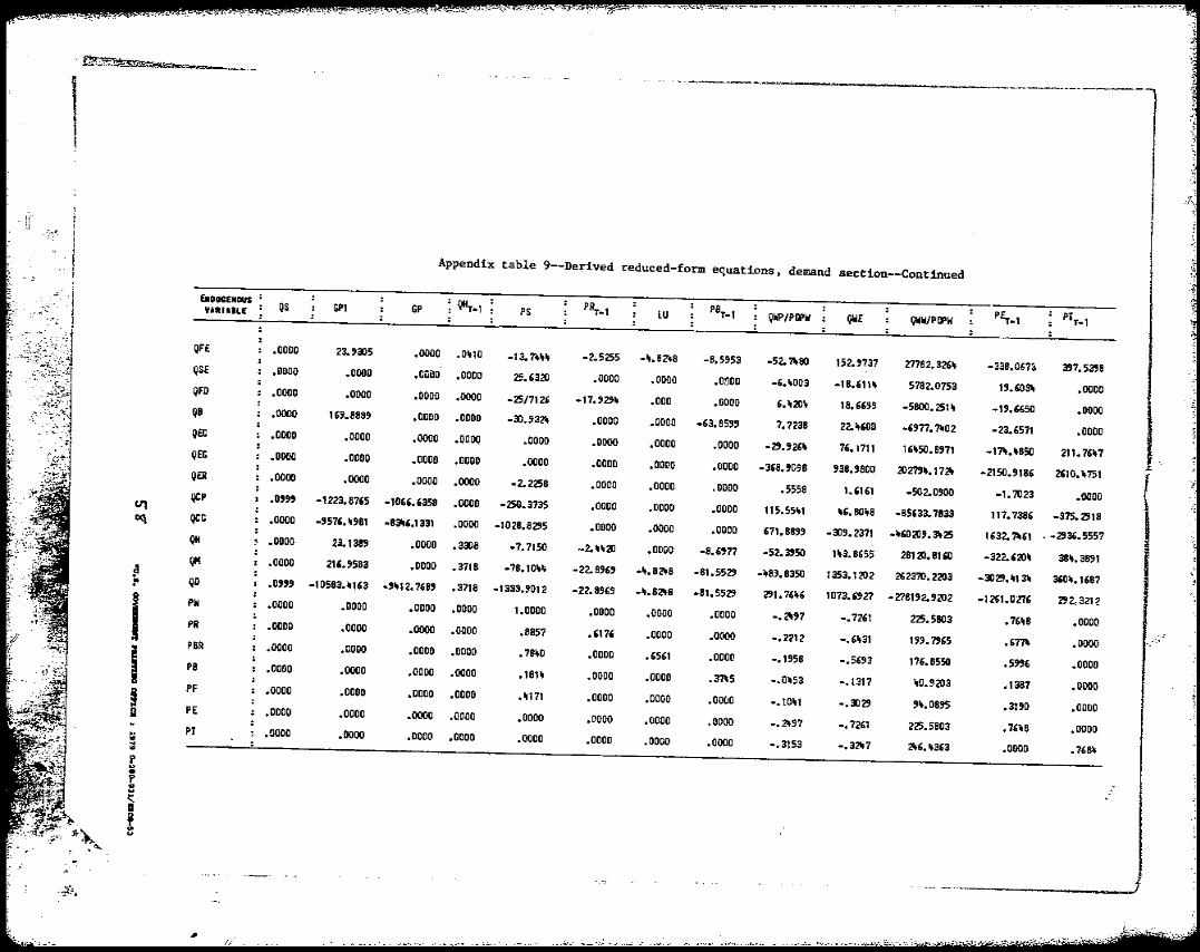
1,

.' I',"1

Appendix table 9--De~ived reduced-form equations, demand section--Continued

EIIDOCENDUS QS GPI PS PO _VARUILE GP ~ QHT-l PR,.-1 lU T 1 PT _QWP/PIPW QWE QWiI/PIPW PEr-l T 1

QFE .0000 23.9315 .0000 .0ltlO -13. 71t~~ -2.5255 -It.821t8 -8.5~53 -52.7't80 152.9737 27782.326~ -338.067~ 397.5398QSE .0000 .0000 •como .0000 25.6320 .0000 .0000 .0000 -6.~003 -18.61n 5782.0753 19.60311 .0000QFO .0000 .0000 .0000 .0000 -25/7126 -17.'~1t .000 .0000 6.lt201t 18.6699 -5800.25n -19.6650 .0000QO .0000 1".8889 .0000 .0000 -31.9321t .0000 .0000 -63.8599 7.7238 22. ~6OD -6977.7't02 -23.6571 .0000QEC .0000 .0000 .0000 .OOOQ .0000 .0000 .0000 .0000 -29.n6~ 76. 1711 16"50.8971 -171t. "850 211.76"7QEG .0000 .0000 .0000 .0000 .0000 .0000 .0000 .0000 -368.9098 1938.9800 20279".17211QER -2150.9186 2610."751.0000 .0000 .0000 .0000 -2.2258 .0000 .0000 .0000 .5558 1.'1'1 -502.0900QCP -1.7023 .0000 I .09" -'223.87'5 -10".'358 .0000 -250.3735VI .0000 .0000 .0000 115.55" 1 "6.80lt8 -85633.7833oq QCG 117.738' -375.2'18

.0000 -957'."981 -8311'.1331 .0000 -1028.82'5 .0000 .0000 .0000 671.8899 -319.2371 -"60209.31125 1632. 7't61 . - 2'36. 5557QH '0 .0000 23. 1389 .0000.3<118 -7.7150

··2.""20 .0000 -8.6977 -52.3950 tlt3.8655 28120.8160 -322. '20" 38". 3891QM .0000 21 ,. 9583 .0000.3718 -78. 1o,,~P -22. 89" -".821t8 -81.5529 -"83.8350 1353.1202 262370.2203

:0 QO -3129."13" 360".1'87.0'" -10583."1'3 ~9"12.7689 .3718 -1333.9012

-22.8969 -".821t8 -81.5529 291.76"6 1073.6927 -278192.9202 -12'1.0276 292.,3212PW •0000 .0000 .0000.0000 1.0000 .0000 .0000 .0000 -.21197 -.7261 225.5803 .76"8 .0000PH .0000 .0000 .0000 .0000 .8857I I.6176 .0000 .0000 -.2212 -.6"31 199.7965 .6771t .0000

I PHR .0000 .0000 .0000.0000 • 78..0

.0000 .6561 .0000 -.1958 -.56'3 176.8550 .5996 .0000PO .0000 .0000 .0000 .0000 .181"

.0000 .0000 .3?1t5 -.0"53 -.1317 "0.9203 .1387 .0000PF .0000 .0000 .0000 .0000 ."171

.0000 .0000 .0000 -.10"1 -.3129 9".0895 .3190 .0000! PE .0000 .0000 .0000 .0000 .0000

.0000 .0000 .0000 -.21197 -.7261 225.5803 .76"8 .0000PT .!l000 .0000to .0000 .0000 .0000 .0000 .0000;;j .0000 -.3153 -.32117 2It6."363 .0000 .768" r.. f

i.. w

~