factors affecting feedlots' decisions on cattle marketing
TRANSCRIPT

South Dakota State University South Dakota State University
Open PRAIRIE: Open Public Research Access Institutional Open PRAIRIE: Open Public Research Access Institutional
Repository and Information Exchange Repository and Information Exchange
Electronic Theses and Dissertations
2017
Factors Affecting Feedlots' Decisions on Cattle Marketing Factors Affecting Feedlots' Decisions on Cattle Marketing
Options: A National Study Options: A National Study
Charlotte Owusu-Smart South Dakota State University
Follow this and additional works at: https://openprairie.sdstate.edu/etd
Part of the Agricultural Economics Commons, and the Economics Commons
Recommended Citation Recommended Citation Owusu-Smart, Charlotte, "Factors Affecting Feedlots' Decisions on Cattle Marketing Options: A National Study" (2017). Electronic Theses and Dissertations. 1154. https://openprairie.sdstate.edu/etd/1154
This Thesis - Open Access is brought to you for free and open access by Open PRAIRIE: Open Public Research Access Institutional Repository and Information Exchange. It has been accepted for inclusion in Electronic Theses and Dissertations by an authorized administrator of Open PRAIRIE: Open Public Research Access Institutional Repository and Information Exchange. For more information, please contact [email protected].
FACTORS AFFECTING FEEDLOTS’ DECISIONS ON CATTLE MARKETING
OPTIONS: A NATIONAL STUDY
BY
CHARLOTTE OWUSU – SMART
A thesis submitted in partial fulfillment of the requirement for the degree
Master of Science
Major in Economics
South Dakota State University
2017


iii
ACKNOWLEDGEMENTS
First, I would like to thank God for how far He has brought me. I also would like
to thank my Advisor Scott William Fausti for his enormous support throughout the writing
process. My committee members, Dr. David Davis and Dr. Matthew Diersen, have also
being of great help.
Special thanks also goes to the Department of Economics for their financial support
in my study at SDSU. I would also like thank South Dakota Association of Economics
students and NIFA for their financial support towards my work.
Last but not least, I would like to thank all my friends especially Kenneth Kwesi
Amoah for making time to edit my work and making constructive suggestions. I am very
grateful for the time, encouragement and support.

iv
TABLE OF CONTENTS
LIST OF FIGURES...………………………………………………………...........v
LIST OF TABLES…………………………………………………………..........vi
LIST OF APPENDICES…………………………………………………………….vii
ABSTRACT.....………………………………………………………………… ...ix
CHAPTER 1: INTRODUCTION
1.1 Background ……………………………………………………………1
1.11 Alternative Marketing Arrangements …………………………… 1
1.12 Thinning Cash Market – Causes and Implications ……………… 4
1.2 Problem Statement …………………………………………………… 9
1.3 Research Objectives and Hypothesis ………………………………...11
1.4 Justification of the study ……………………………………………. 13
CHAPTER 2: LITERATURE REVIEW
2.1 Literature on Benefits and Impacts of Captive Supplies …………… 15
2.2 Literature on Concentration and Market Power ……………………. 19
2.3 Literature on Mandatory Price Reporting …………………………... 22
2.4 Literature on Price Transparency and Price Discovery …………….. 30
CHAPTER 3: DATA DESCRIPTION AND METHODOLOGY
3.1 Data Sources ………………………………………………………... 34
3.2 Theoretical Foundation ……………………………………………... 36
v
3.3 Econometric Model …………………………………………………...39
3.4 Regression Diagnostics …………………………………………….....44
3.41 Stationarity Test ……………………………………………..44
3.42 Serial correlation test ………………………………………..46
3.43 Heteroscedasticity …………………………………………...48
3.44 Multicollinearity …………………………………………….48
3.5 Estimation Techniques ……………………………………………… .48
CHAPTER 4: RESULTS AND ANALYSIS
4.1 Summary Statistics ………………………………………………….. 51
4.2 Discussion on Regression Analysis …………………………………. 52
4.3 Results from Diagnostic Tests ………………………………………..58
4.31 Results from Residual Correlation Matrix …………………..58
4.32 Results from Endogeneity Test ……………………………...59
4.33 Results from stationarity Test ……………………………….60
4.34 Results from Serial Correlation Test ………………………...60
4.35 Results from heteroscedasticity Test ………………………...60
CHAPTER 5: CONCLUSIONS …………………………………………………..62
REFERENCES ……………………………………………………………………66
vi
LIST OF FIGURES
Figure 1: Summary of Marketing and Pricing Methods in Cattle market ………... 2
Figure 2: Trends of Market Shares for Fed Cattle ………………………………... 7
Figure 3: Cattle Transactions on Live Basis ……………………………………… 7
Figure 4: Cattle Transactions on Dressed Basis ………………………………….. 8
vii
LIST OF TABLES
Table 3.1: Description of Variables …………………………………………....... 35
Table 4.1: Summary Statistics ………………………………………………....... 52
Table 4.2: SUR for Cash versus Formula Market ………………………………. 53
Table 4.3: SUR for Cash versus Forward Contract Market …………………….. 56

viii
LIST OF APPENDICES
Appendix A: Stationarity test for residuals …………………………………….. 81
Appendix B: Results from residual versus fitted plots …………………………..82
Appendix C: Error Correlation Matrix ………………………………………… .84
Appendix D: Results from Augmented Regression Test ………………………. 85
Appendix E: Test for Serial Correlation …………………………………………86
Appendix F: Stationarity test for variables ………………………………………87
Appendix G: Robust OLS for Forward Contract Market ………………………..88
Appendix H: Robust OLS for Formula Market ………………………………….89
ix
ABSTRACT
FACTORS AFFECTING FEEDLOTS’ DECISIONS ON CATTLE MARKETING
OPTIONS: A NATIONAL STUDY
CHARLOTTE OWUSU-SMART
2017
This thesis investigates the economic implication of changing slaughter volume
patterns across the cash and contract markets in the US cattle industry. Weekly time series
data that spans from November 2002 to December 2015 was used in the analysis. Empirical
evidence suggests that Mandatory Price Reporting (MPR) played an important role in
changing slaughter volumes across the cash and contract markets. Additionally, price of
feeder cattle, cattle quality characteristics (Choice-Select spread and the percentage of
animals grading choice or better) among others influence feedlots’ decision to use a
particular marketing arrangement.
Key words: AMA, MPR, SUR, cattle, cash market, formula market, forward contract
market, thinning market, price discovery.

1
1.0 CHAPTER ONE: BACKGROUND OF STUDY
1.1 ALTERNATIVE MARKETING ARRANGEMENTS
Cash market transactions are transactions that occur immediately or “on the spot”.
They may include sales through other buyers, dealers or brokers; direct sales and auction
barn sales (Taylor et. al, 2007). All possible alternatives to the cash market are termed
Alternative Marketing Arrangements (AMAs). Apart from the fact that AMAs are
alternatives to the cash market, they all (except packer ownership) involve delivery of
contracted cattle at least 2 weeks after the contract was entered into. AMAs may, however,
vary in terms of their ownership method, pricing method or valuation method.
The ownership method defines who owns the cattle at the time of transaction; the
pricing method shows how transaction prices were established and the valuation method
tells whether or not cattle characteristics were considered in the final transaction price. If
cattle characteristics were considered, then grid premiums and or discounts would apply
(Taylor et. al).
Forward contracts are similar to cash markets since there is a bid and ask on prices
except that cattle are delivered at least two weeks after the agreement was entered into.
Formula trades are the most widely used AMAs. Prices used in formula transactions are
determined using a base rather than prices dictated by agents involved in the transaction
(Koontz, 2013). Sources of base prices used in formula trades of fed cattle may include
average regional prices, USDA AMS1 regional prices, plant average prices and national
average prices. The final formula price for a given transaction is composed of a base price
1 United States Department of Agricultural (USDA), Agricultural Marketing Service (AMS).
2
plus or minus premiums or discounts depending on cattle quality. Until 2004, negotiated
grid trades were considered as part of formula trades since they all involved the use of a
formula to determine prices. The main difference, however, is that formula trading relies
on external market indicators to determine prices while the negotiated grid system
sometimes uses these formula prices as a base prices. For the purpose of this discussion,
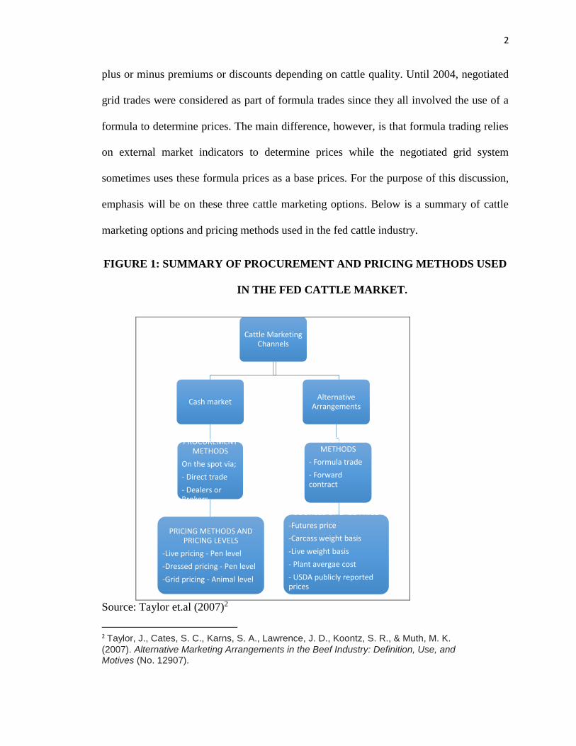
emphasis will be on these three cattle marketing options. Below is a summary of cattle
marketing options and pricing methods used in the fed cattle industry.
FIGURE 1: SUMMARY OF PROCUREMENT AND PRICING METHODS USED
IN THE FED CATTLE MARKET.
Source: Taylor et.al (2007)2
2 Taylor, J., Cates, S. C., Karns, S. A., Lawrence, J. D., Koontz, S. R., & Muth, M. K.
(2007). Alternative Marketing Arrangements in the Beef Industry: Definition, Use, and Motives (No. 12907).
Cattle Marketing Channels
Cash market
PROCUREMENT METHODS
On the spot via;
- Direct trade
- Dealers or Brokers
PRICING METHODS AND PRICING LEVELS
-Live pricing - Pen level
-Dressed pricing - Pen level
-Grid pricing - Animal level
Alternative Arrangements
PROCUREMENT METHODS
- Formula trade
- Forward contract
SOURCES OF BASE PRICE
-Futures price
-Carcass weight basis
-Live weight basis
- Plant avergae cost
- USDA publicly reported prices

3
There have been significant changes in the U.S livestock market which includes but
is not limited to the increased use of AMAs (as against the cash or spot market) by feedlots
to market their livestock (Kim and Zheng; 2015). Over the past few decades, there has been
a gradual transition from the use of the cash market to the use of AMAs to sell fed cattle.
This is because of the increased advantages AMAs possess and may include: higher and
predictable volumes, relatively lower transportation costs as compared to cash markets,
higher capacity utilization, and their demand enhancing ability (Koontz, 2013). Also, in
the 2007 Grain Inspection, Packers and Stockyards Administration (GIPSA) report,
producers and packers were asked the three most important reasons for either using AMAs
or cash markets. About 51.6% of producers used AMAs because it allows the sale of higher
quality cattle. Again, 16.3% of the respondents also used cash markets because of its higher
prices which reflected higher cattle quality.
AMAs that result in captive supplies of livestock by packers (i.e. control or
ownership of livestock more than 14 days prior to slaughter) have raised particular
concerns for many industry participants. For this reason, in 2003, Congress funded research
that was based on the potential costs and benefits that AMAs might have on the meat and
livestock industries. The study was completed in early 2007, and the results are being used
in discussions about policy changes that are needed to address whether the use of particular
methods of procuring livestock by packers had adverse effects on the livestock and beef
industries (Taylor et al).
The fact still remains that the use of AMAs is relatively advantageous to both
feedlots and packers. This, however, does not justify the displacement of the cash market
4
(Koontz, 2013). The cash market still plays an important role because, at the very least, it
enhances the price discovery3 mechanism that aids the determination of prices for most
AMAs especially formula-based prices.
1.12 THINNING CASH MARKET- CAUSES AND IMPLICATIONS
Most agricultural markets in the United States have experienced increased
concentration over the past two decades. The concentration of the livestock industry has
been incentivized by vertical coordination4, change in consumer preferences and
technological advancement.
Discussing vertical coordination, firms that use a competitive strategy aim at
operating at the lowest average cost as possible (Boland, Barton and Domine, 1999). For
this reason, beef packers have increasingly entered into contracts with feedlots to ensure a
steady supply of fed cattle so they can operate at full capacity. This makes the livestock
industry concentrated as it results in the formation of very large firms.
With reference to changes in consumer preferences, rising incomes, over the years,
have led to changes in demand patterns. Even though this has created market for most
producers, it has further concentrated the industry since fewer producers “fill each niche”
(Adjemian et al, 2016). Historically it has been noted that, the four firm concentration
3 Price discovery is the process by which buyers and sellers use available market information to determine the price for a given transaction. It involves two market participants (buyers and sellers) to arrive at a price taking into account the quantity and quality of the commodity being traded (Ward and Schroeder, 2002). 4 Vertical coordination is said to have occurred when firms in different stages of production work together to achieve an economic goal (Harkin, 2004).
5
ration (CR45) for fed cattle increased from 36% to 81% from 1980 to 1993 and has
increased marginally since then6. Concentration in the beef industry can be problematic
when it results in the exercise of market power by beef packers. Perloff and Rausser (1983)
argue that firms that exercise market power are able to control prices and can cause
economic losses to other market participants. Below is a chart that shows the trend of the
concentration ratio in the US fed cattle industry.
Between 1980 and 2010, concentration in the cattle industry has risen by more than
100% (USDA ERS, 2012). The increase in concentration was sharp between 1980 and
1995, however concentration increased marginally thereafter. The recent thinning7 of the
cash market, however, is attributable not only to concentration in the livestock industry but
also to the gradual transition from the use of the cash market to contract markets. In packers
or processors quest to satisfy downstream demand, they seek better coordination from the
sources of their inputs. To further improve the quality of coordination, market participants
resort to the use of contracting. According to MacDonald and Korb (2008) the use of
contracts offer several advantages to feedlots. Some of which include: serving as a risk
management tool, assuring feedlots of a market for their cattle and rewarding (through
premiums) feedlots who provide the quality characteristics stated in the contracts. The
5 CR4 simply means four-firm concentration ratio. It measures market concentration by combining the market shares of the four largest firms in the industry. According to Wise and Trist (2010), when CR4 is 20%, the market is concentrated; a CR4 of 40% means that the firm is highly concentrated and 60% and beyond means there is a possibility of firms to exercise market power. A CR4 of 20% means that 20% of the market is being controlled by 4 largest firms. 6 For details on concentration in the livestock industry, see the Concentration in Agriculture report (U.S. Government Accountability Office, 2009). 7 A market can be said to be thin when there is a small number of buying or selling offers. It is usually characterized by high price volatility, low trading volumes, higher searching and bargaining costs (Rostek and Weretka, 2008).

6
packing industry benefits include the ability to manage their input supply chain and to
maintain their plants at full capacity. AMAs are thought to be beneficial to market
participants, otherwise, they would not use it. Koontz (2013), however, discussed that a
considerable increase in the use of contracts may go a long way to affect the cash market
negatively. Koontz argues that the process of price discovery is enhanced by increased
transactions in the cash market. Thus, for an effective and efficient price discovery process
there should be enough transactions to accurately reflect market activities.
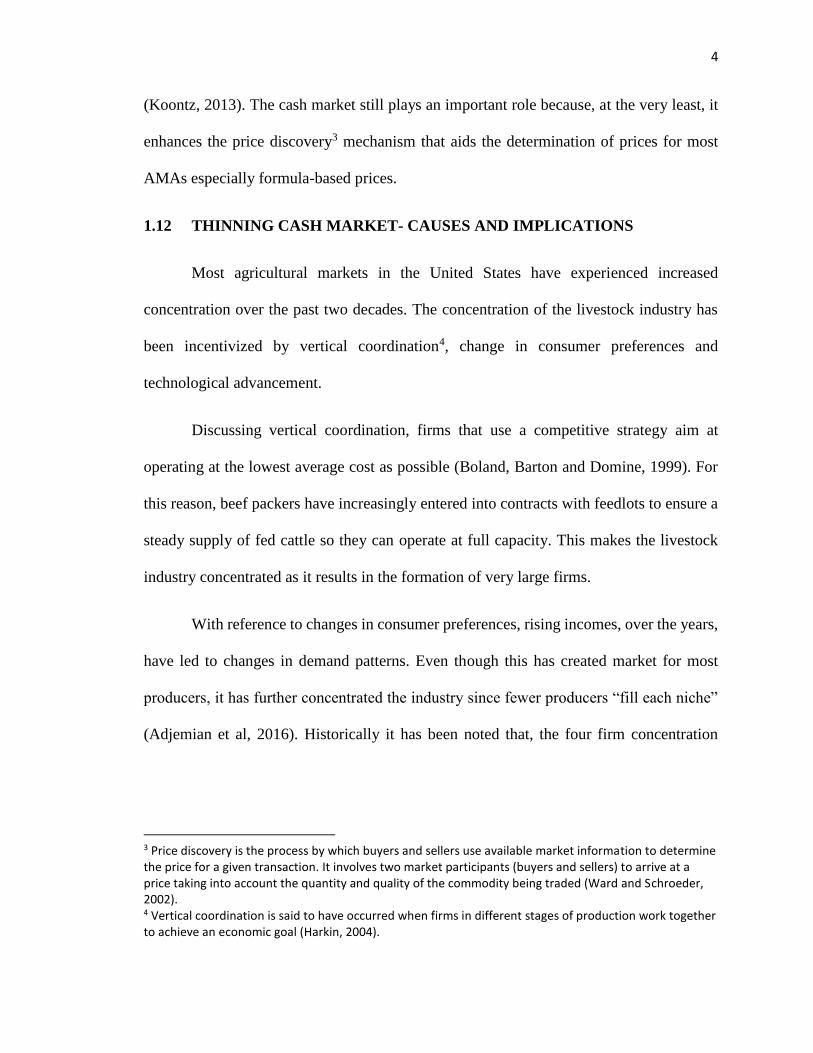
Figure 2 shows trends of markets shares under the four major marketing options. It
confirms that the fed cattle market, over the years, has experienced an enormous shift from
the use of conventional cash markets to the use of contracts – formula trade and forward
contracts. Negotiated grid sales, however, have seen little or no changes in volume shares
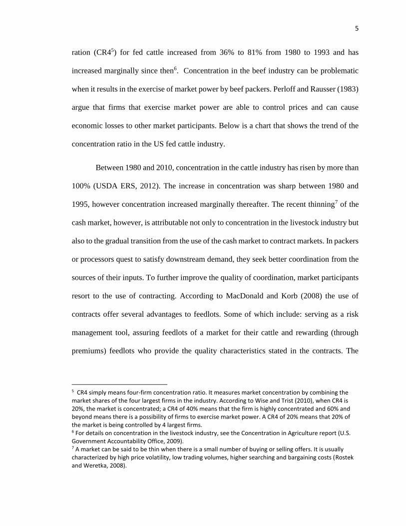
over the course of time. These trends slightly differ for both the live and dressed-weight
market. For this reason, figure 2 was further broken down into transaction on live and
dressed basis for the various marketing arrangements. Figure 2 indicates that there has been
a steady decline in cash market sales over the past few decades. Most of the shift in market
shares favored formula trade. There has also been a slight increase in forward contract
shares over time. The decline in the cash market is also evident in figure 4. It is, however,
slightly different from what was seen in figure 2.

7
FIGURE 2: TRENDS OF MARKET SHARES FOR FED CATTLE
Source: Livestock Marketing Information Center (LMIC)
FIGURE 3: CATTLE TRANSACTIONS ON LIVE BASIS
Source: Livestock Marketing Information Center (LMIC)
0.00%
10.00%
20.00%
30.00%
40.00%
50.00%
60.00%
70.00%
80.00%
04
/08
/01
11
/08
/01
06
/08
/02
01
/08
/03
08
/08
/03
03
/08
/04
10
/08
/04
05
/08
/05
12
/08
/05
07
/08
/06
02
/08
/07
09
/08
/07
04
/08
/08
11
/08
/08
06
/08
/09
01
/08
/10
08
/08
/10
03
/08
/11
10
/08
/11
05
/08
/12
12
/08
/12
07
/08
/13
02
/08
/14
09
/08
/14
04
/08
/15
11
/08
/15
Vo
lum
es in
Per
cen
tage
s
Weeks
Market Shares
Negotiated Negotiated Grid Formula Forward Contract
0.00%10.00%20.00%30.00%40.00%50.00%60.00%70.00%80.00%90.00%
100.00%
11
/24
/02
06
/24
/03
01
/24
/04
08
/24
/04
03
/24
/05
10
/24
/05
05
/24
/06
12
/24
/06
07
/24
/07
02
/24
/08
09
/24
/08
04
/24
/09
11
/24
/09
06
/24
/10
01
/24
/11
08
/24
/11
03
/24
/12
10
/24
/12
05
/24
/13
12
/24
/13
07
/24
/14
02
/24
/15
09
/24
/15P
erce
nta
ge o
f tr
ansa
ctio
ns
Date
LIVE BASIS
Negotiated Negotiated Grid Formula Forward Contract

8
Figure 3 shows that, even though cash transactions for the live market are declining
over the years; the cash market still remains dominant relative to the other AMAs as far as
the live market is concerned. Schroder et. al (2009) argued that the live market is mostly
used by those producers who are not sure of the quality characteristics of their cattle. They
further explained that if producers expect the quality of their cattle to be lower than average,
they are motivated to sell on the live rather than the dressed market.
Fausti and Qasmi (2002) also explained that producers who are risk averse and do
not meet the minimum quality characteristics prefer to sell on an average price basis rather
than on a grid. In the same light, most producers who use the cash market are not concerned
about quality characteristics. This further explains why the cash market is dominant when
selling cattle on live basis
FIGURE 4: CATTLE TRANSACTIONS ON DRESSED BASIS
Source: Livestock Marketing Information Center (LMIC)
0.00%
10.00%
20.00%
30.00%
40.00%
50.00%
60.00%
70.00%
80.00%
90.00%
11
/24
/02
05
/24
/03
11
/24
/03
05
/24
/04
11
/24
/04
05
/24
/05
11
/24
/05
05
/24
/06
11
/24
/06
05
/24
/07
11
/24
/07
05
/24
/08
11
/24
/08
05
/24
/09
11
/24
/09
05
/24
/10
11
/24
/10
05
/24
/11
11
/24
/11
05
/24
/12
11
/24
/12
05
/24
/13
11
/24
/13
05
/24
/14
11
/24
/14
05
/24
/15
11
/24
/15
Per
cen
tage
of
tran
sact
ion
s
Date
Dressed basis
Negotiated Negotiated Grid Formula Forward Contract

9
Dressed weight pricing was not more popular relative to live weight pricing. Feuz
et al (1993) asserted that this was because there is a time lag between the sale and
procurement of animals under the dressed weight marketing option. Most dressed weight
prices are similar to live prices in the sense they all start off with a base price and are further
adjusted for weight premiums and discounts, yield and quality grades, slaughter cost and
so on (Schroder et al). Dressed-weight prices can be compared to live-weight prices after
adjusting for dressing percentage. However, dressed weight cattle sold by the pen will
receive the same price per hundredweight.
According to Feuz et al, dressed weight system (except for cattle sold by the pen8)
is value based and it rewards quality cattle. It is, therefore, expected marketing option that
takes into account quality measures will dominate the dressed-weight market. Figure 4
shows that formula trade transactions are dominant with the dressed weight pricing option.
1.2 PROBLEM STATEMENT
A market is said to be transparent when all market information deemed relevant is
made available to market participants. In an economic sense, relevant information may
include information on both price and quantities traded to determine the market price for a
given commodity. Price transparency, therefore, is making transaction prices available to
all market participants. This has the advantage of resulting in efficiency in price discovery,
reducing the incidence of arbitrage opportunities and increasing integration between spatial
markets (Pendell & Schroeder, 2006).
8 Cattle sold by the pen will receive the same price per hundredweight.

10
Prior to the Mandatory Price Reporting Act of 1999, the Voluntary Price Reporting
(VPR) system was the primary source of public information on livestock market activity.
This system allowed producers, feedlot operators and packers to voluntarily report prices
and respective quantities for the various sale/procurement methods they used. Over time,
both feeders and packers began to resort to the use of alternatives to the cash market. These
other methods, however, did not have prices and volumes reported. In other words, a
framework had not been established to report these prices. Also, given the heterogeneous
nature of the pricing and valuation methods that were in use, it was not possible for market
reporters to collect price information for the variety of sales through the informal survey
methods they were using (Ward and Schroeder, 2002). This made the accuracy of the prices
used on the cash market questionable since it did not reflect all on-going cattle transactions.
There were various criticisms regarding the use of the VPR system as prices and
quantities reported did not reflect what was happening in reality. Market transparency was
degraded and market agents behaved strategically when they voluntarily reported prices
(Fausti and Diersen, 2003). Without price information there will be no historical basis upon
which risk management policies will be formulated (Koontz, 2015). In an attempt to
increase competition, make prices reflect all cattle trade, and more importantly, improve
price discovery; Congress passed the Livestock Mandatory Price Reporting (LMR) Act of
1999. The LMR policy proposal was strongly contested by packing industries but was
supported by producers. The system, however, took effect from April 2001 and mandated
meatpackers to report daily transactions of their livestock to the Agricultural Marketing
Services (AMS).

11
Various studies (Schroeder, Grunewald & Ward 2004; Koontz 2013; Ward, Vestal
and Lee 2014) have observed downward trends in the use of the cash market since the
implementation of the MPR. Increased transparency has led to renewed interest and focus
on thin markets (Ward, Vestal and Lee 2014). The thinning of the cash market has raised
concerns regarding the accuracy of prices reported on the cash market. Another concern
that Ward (2008) raised is that prices in thin markets are subject to greater potential
manipulation than in more heavily traded markets. Are these prices representative of the
interaction between market forces? How thin can the cash market be so that the prices
discovered are still accurate? How thin can the cash market get so that the price discovery
mechanism is still efficient? Most parts of literature on this subject matter have looked at
the trends of the cash market and AMAs before and after the inception of MPR
(Wachenheim and DeVuyst (2001); Koontz (2013); Ward (2014); Ward, Vestal and Lee
2014).
In addition, concentration in the fed cattle industry has led to decreased competition
among packers. A reduction in competitive activities also serves as breeding grounds for
certain market participants to exercise power. In the case of the fed cattle industry, packers
who exercise market power may increase their profits by reducing the prices they pay to
feedlots. The issue of thin cash markets results in insufficient data for market participants
to analyze the accuracy of information on the market. Feedlots, for this reason, doubt
whether they receive fair prices in the face the thinning cash market (Adjemian et al., 2016).
In an effort to add to existing knowledge, this study attempts to explore the potential
causes of the shift from the use of the cash market to contract markets. Specifically, it seeks

12
to find out the possible factors that encourage or prompts market participants to use
contracts instead of the conventional cash market beyond rational provided in the current
literature9.
1.3 RESEARCH OBJECTIVES AND HYPOTHESES
This study generally seeks to examine factors responsible for the shift from the use
of cash markets to the use of AMAs. Economic factors suggested in the literature are
empirically tested. One controversial casual factor being tested is whether or not MPR
played a role in the decline of cash market volume over the period under study. The
influence of MPR is of interest because it is a major policy change that occurred in the US
livestock industry since 2001. There is a branch of the MPR literature that argues that MPR
could result in a change in marketing behavior in the fed cattle market. Anecdotal evidence
in support of this view is that use of cash market also occurred around the same time. This
provides a basis to the believe that MPR might partly be responsible for the gradual shifts
to the use of AMAs. To account for this in the analysis, MPR is defined as a dummy
variable that takes on the value of one in periods when MPR was enforced and zero in
periods when MPR was not active.
The strawman assumption behind the MPR dummy variable is that the introduction
of MPR did not affect volumes shares of marketing arrangements in any way. Or, even if
it did, the effect was insignificant. The reverse is true for the alternative hypothesis.
9 Recent studies show that market participants use AMAs instead of the cash market because of the many advantage AMAs provide. [Ward and Schroeder (2004); Franken et al (2009); Koontz (2007)] argue that some reasons why feedlots and packers use AMAs include: lower transaction costs, higher and predictable volumes and reduction of potential risk.
13
Rejection of the null hypothesis will mean that the introduction of MPR had a significant
effect on volumes shares. A rejection of the null hypothesis will imply that volume shares
in the contract market increased in periods when MPR was enforced.
1.4 JUSTIFICATION OF THE STUDY
Agricultural commodities experience relatively higher price variations than other
non-farm goods (Tomek & Robinson, 2003). These variations can be attributed to market
forces coupled with the production process. Economists and other financial stakeholders
have recognized price fluctuations as an important economic phenomenon that affects most
decision-making on prices. This complicates price discovery and implies risk to many
economic agents.
The AMA literature has shown that most AMA prices are related to cash market
prices. For instance, the base prices used in formula prices are frequently tied to last week’s
cash market in some way (Ward, Vestal & Lee, 2014). In this regard, prices dictated by the
cash market should be as accurate as possible since there is a spillover to other markets.
The recent concern regarding the thinning of the cash market and the accuracy of cash
prices have necessitated studies that seek to find out the causes of this problem.
Results from this study will provide information relevant to policy making in the
fed cattle industry. Policy officials working on policies geared towards tackling specific
problems may find insight on how price discovery and market transparency can be
improved once the questions to these objectives are answered. Specifically, results from
this study will give insight as to how MPR has affected volume shares of the cattle
marketing options under consideration.

14
This thesis was divided into five chapters. Chapter 1 covers the introduction,
research objectives and the justification of the study. Chapter 2 is a review of previous
literature related to cash market thinning. Chapter 3 describes the datasets and the research
methodology used. Analysis of empirical results corresponding to the research objectives
is presented in Chapter 4. Conclusions from the study and necessary recommendations are
provided in Chapter 5.

15
2.0 CHAPTER 2: LITERATURE REVIEW
This section provides literature on the main tenets of this paper. It covers literature
on Alternative Marketing Arrangements, Mandatory Price Reporting, Concentration in the
livestock industry, market transparency and price discovery.
2.1 LITERATURE ON BENEFITS AND IMPACTS OF CAPTIVE SUPPLIES
GIPSA defines captive supply as livestock that is procured by packers for more
than two weeks before slaughter. In other words, captive supply can be referred to as
livestock that are procured through a contract, which was entered into at least 14 days
before slaughter. The rising concern about the use of captive supplies resulted in a
legislation proposed as part of the 2002 Farm Bill to ban packer procurement of cattle
through captive supplies. In the fall of 2007, the Senate Agriculture Committee passed an
amendment that would have prevented packers from owning cattle for more than two
weeks before slaughter. The share of livestock procured through captive supplies is on the
increase and has raised concerns about thinning cash markets and its unexpected
consequences. In the case of cattle, cash transactions declined from more than 60% in 2004
to less than 30% in 2014 (Adjemian et. al, 2016). About 36% of hogs were transacted on
the cash market in 1999, however, this share had decreased to 24% by 2004 and 2005
(Grimes and Plains, 2009). These trends do not only show producer-packer preference for
non-cash transactions but also draws attention to the potential to erode price transparency
and price discovery in the cash market.
There are two Congressionally-mandated studies on captive supplies. The first
study was done by Ward, Koontz and Schroeder in 1996 and the second study was Taylor

16
et. al (2007). Both studies were focused on evaluating the cost and benefits from the use of
AMAs. Using data from April 1992 to April 1993, the 1996 study found that the use of
AMAs reduces cash prices by at most 1.2%. The 2007 study found that the use of AMAs
reduced cash prices by at most 0.3%. Authors of the 2007 paper also found that the cost of
using AMAs was about $4.50 per head while gains from the use of AMAs were estimated
to be $6.50 per head. They concluded that the overall benefits from the use of AMAs
outweighed costs.
Schroeter and Azzam (1996) used data on cattle procurement for the four largest
packing firms in Texas, Panhandle from February 1995 to May 1996 to assess the effect of
AMAs on cash prices. They found that when packers anticipate large deliveries of AMA
cattle, they are motivated to pay lower prices in the cash market. Schroeter and Azzam
found that a 10% increase in AMA deliveries is associated with a $0.021/cwt lower cash
price. They explained further that if the source of the base price is USDA reported prices,
it will be nearly impossible for packers to manipulate cash prices. However, if the source
of the base price is from the plant average cost, then it would be easier to manipulate prices
paid for formula-priced cattle. They argued that whether or not AMA deliveries affected
cash prices depended on the type of base price used in formula pricing. Crespi and Sexton
(2004) also used transaction data on Texas Panhandle region to examine market
competitiveness with reference to the procurement of captive supplies. They found that
captive supplies allow packers to reduce cash bids by 5-10%.
Hayenga and O’Brien (1991) used a 15-month period data from October 1988 to
December 1989 to examine the effect of captive supply deliveries on weekly fed cattle

17
prices. They found no evidence to support the claim that forward contracts negatively
affected fed cattle prices. Elam (1993) also used monthly average fed cattle data from
October 1988 to May 1991. The main aim of the study was to examine the effects of captive
supply deliveries on fed cattle price in Kansas, Colorado, Texas, Nebraska and the United
States as a whole. Elam found an inverse relationship between fed cattle prices and captive
supplies. Results from Elam’s time series analysis suggested that impacts of captive
supplies on fed cattle price differed from state to state. Elam found that the impact of
captive supplies on cattle prices ranged from no significant impact to about $0.37/cwt.
Ward et al (1998) found rather mixed but interesting results. They found that the
relationship between total inventory of captive supply was generally negative for the period
they examined. These results, however, differed based on the marketing arrangement under
consideration. Captive supplies associated with the forward market had a positive impact
on cash prices while marketing arrangement inventory constantly showed a negative
relationship with cash prices.
Ward and Schroeder (2004) concluded that AMAs are beneficial to both cattle
producers and packers or else they would not use them. The concern of most market
participants in the industry is how AMAs might affect suppliers who prefer to deal on cash
basis. Procuring cattle through AMAs effectively reduces the supply of cattle on the cash
market that can be purchased by other buyers. Also, packers without captive supplies need
to bid more aggressively on the cash market for the limited supply of cattle (Ward and
Schroeder, 2004). Both of these scenarios should push the prices of fed cattle up. However,
it also means that packers who have met most of their supply needs through captive

18
supplies need not bid aggressively on the cash market and this may cause a decline in the
market price of fed cattle.
Research by USDA GIPSA (1996) and Schroeter and Azzam (2003) have also
confirmed that the net effects of the increased use of captive supplies on short run prices
paid for cattle on the cash market is negative but small. Kim and Zheng (2015) specified a
model which defines two ways through which captive supplies may affect the spot price in
livestock markets. They found that increases in the number of hogs procured through
AMAs increases cash price volatility and the cash price level. They further decomposed
the effect on the price level into direct effects and indirect effects. The direct effect,
according to their model, results from the increase in the number of hogs procured through
AMAs. This causes packers to bid less aggressively in the cash market thus causing a
reduction in demand rather than supply in the cash market. Kim and Zheng concluded that
this represented a structural change that favored packers. Wang and Jaenicke (2006),
however, argued that the reason for low cash prices is that captive supplies divert livestock
of good quality away from the cash market. If that is the case, then the issue of low cash
prices is less problematic as it simply reflects that fact that low quality livestock commands
low prices.
Another branch of the AMA literature discusses the benefits and potential
motivations involved in the use of captive supplies. Franken et. al (2008) stated that both
risk preferences and transaction costs are important in determining a packer’s choice of
procurement method. Other papers show that efficiencies exist where packers with more
captive supplies operate at higher volumes, have less variability in slaughter volumes,

19
lower average cost and higher average margins per head. For example, Key and McBride
(2003) specifically show that one of the main reasons why packers use captive supplies is
that they can reduce transaction costs by contracting with fewer and larger feedlots. Ward
and Schroeder (2004) also identified potential motivations behind why cattle feeders use
contract markets. Risk management, obtaining favorable financial terms and securing a
buyer(s) for their cattle were some of the reason they stated. On the other hand, the cash
market exhibits economies of scale and as the cash market thins, producers may incur
higher transaction costs that may make the use of cash markets less attractive. Koontz
(2007) also stated that higher predictable volumes and lower average costs are some of the
reasons why packers would want to use captive supplies. Whitley (2002) also found that,
on average, a greater percentage of cattle procured through AMAs is positively related to
a higher beef quality. However, a relationship between beef quality and the use of certain
marketing channels has not been established.
2.2 LITERATURE ON CONCENTRATION AND MARKET POWER
As discussed in Chapter one, one of the structural changes that the US livestock
industry has undergone over the past few decades is increased firm concentration. A major
concern with regards to concentration in the beef industry is the inadequacy of competition
among buyers and its effects on fed cattle prices.
Ward and Schroeder (2004) defined concentration as a measure of the market
dominance by few large firms. High concentration levels are usually associated with lower
prices paid for inputs and higher prices charged for outputs. Impacts of high concentration
are difficult to measure. Cattle suppliers raise concerns about not having a market for cattle
20
when they reach market weight, receiving lower prices for livestock and inadequate
competition among buyers.
Azzam and Schroeter (1995) assessed the tradeoffs in gains from efficiency and
loss from market power that results from concentration in the beef packing industry. They
found that cost savings of at most 2.4% from efficiency gains can offset a 50% increase in
concentration that results in market power. They, therefore, concluded that the net effect
will be positive as efficiency gains outweighed losses from market power. Azzam (1997)
extended the work of Appelbaum (1982) and clearly distinguished market power effects
that are due to concentration from effects due to cost efficiency. He also found that
concentration of packers is associated with both costs and benefits, which yielded positive
net effects. He concluded that his analysis provided empirical confirmation of the trade-off
between cost efficiency and market power that results from packer concentration. Paul
(2001) also used monthly plant-level cost and revenue data from 1992 to 1993 to estimate
Oligopsony and Oligopoly power for beef packing plants. This study found significant
evidence of economies of size and little evidence in support of market price distortions.
Several studies have also used different approaches and varying sources of data to
test whether there is evidence that beef packers exercise market power. The overall
conclusions with regards to the extent and impacts of market power on the cattle industry
as a whole is, however, mixed.
Schroeter (1988) used the conduct parameter approach to assess the degree of
market power in the beef packing industry. He found that monopoly and monopsony price

21
distortions10 were small but statistically significant. Koontz, Garcia and Hudson (1993)
modified the conduct parameter approach by featuring a dynamic pricing game. They
found that market power is found in daily fed cattle prices and price distortion ranges
between 0.5% and 0.8%. They, therefore, concluded that cooperative price behavior among
meatpackers in procuring cattle is indicative of oligopsonistic power. Stiegart, Azzam and
Brorsen (1993), however, stated that reducing concentration in the cattle industry is
unlikely to increase fed cattle prices. Koontz and Garcia (1997) extend the 1993 paper to
include multiple regional markets. Oligopsony behavior was found across multiple
geographic (regional) fed cattle markets.
Zhang and Sexton (2000) used a spatial model and a noncooperative game approach
to show how meatpackers use captive supplies to strategically influence cash prices. They
find that captive supplies can create geographic buffers that reduce competition among
processors. Xia and Sexton (2004) also examine the competitive implications of the
contract arrangements on the cash market. They focused on “top-of-the-market-pricing”
(TOMP) which is commonly related to AMAs. They found that buyers who purchase cattle
on contract also compete to procure cattle in the cash market. They, however, noted that
the use of captive supplies reduces packers’ incentive to compete in the cash market.
For the purposes of testing the existence of market power on the cash market and
whether the source of that market power could be related to the use of captive supplies,
Vukina and Zheng (2009) modelled market power as a function of packers’ stock of captive
10 Monopoly price distortions refer to observing prices that are higher than competitive prices for wholesale
meat sold by packers. Monopsony price distortions, on the other hand, refer to observing prices that are
lower than competitive prices for livestock purchased for slaughter by packers.

22
supplies. They found a statistically significant presence of market power in the
procurement of live hogs on the cash market. They, however, concluded that the source of
market power could not result from captive supplies only; it could also stem from the
concentration of meat packers in the industry. Ji (2011), in one of his three essays on
market power, used a New Empirical Industry Organization (NEIO) model. He extended
the work of Azzam (1997) by including the effects of captive supplies on market power.
He estimated the conjectural variation elasticity, which measures how market power
responded to changes in concentration, captive supplies and their corresponding cost-
efficiencies. He concluded that captive supplies and packers’ concentration were sources
of market power in the beef industry; however, their benefits exceeded costs and hence
improved social welfare.
2.3 LITERATURE ON MANDATORY PRICE REPORTING
The voluntary pricing system was used to report prices and volumes before 2001.
This system allowed buyers and sellers to report market prices willingly. Confirmations
were required by both buyers and sellers by Agricultural Marketing Service (AMS)
reporters before transactions were included in market summaries. It was basically a
communication between reporters and market participants to provide market summaries on
prices and volumes. The Livestock Mandatory Report Act (LMR) was passed in 1999 and
allowed the USDA AMS to implement a mandatory price reporting system which took
effect in April 2001. The main goal of the Act was to facilitate marketing by providing
information about what transpired in the market and to ensure transparent price discovery.

23
According to the US Senate report in 1999, the Act required packers that slaughter
greater than 125,000 cattle yearly to give reports on transactions twice daily. Prices paid
for cattle and the marketing arrangement(s) under which they were sold were also supposed
to be part of the reports. The passage of MPR was accompanied by new reports and an
increase in the amount of information available to market participants. The Act was
reauthorized in 2010 and expired in September 30, 2015. According to Scott Shearer of the
Bockony Group in Washington D.C., the Act has currently being reauthorized and is set to
expire on September 30, 2020.
Proponents of the mandatory system argued that the voluntary price system was no
longer reliable due to the decline of terminal livestock markets and an increase in
concentration in the livestock industry (Keimig et. al, 2002). Feeders and packers also had
rapidly adopted the use of AMAs to market cattle, a portion of on-going transactions that
were not included in market summaries under the voluntary system. The transition from
the use of cash markets to the use of contracts reduced the amount and quality of
information that were available to both feedlots and packers (Perry, 2005). These raised
concerns among cattle producers about the advantages meat packers could be enjoying to
their detriment.
There is a considerable amount of literature that discusses the implications of
MPR11 and its effects on the livestock industry. A large component of this literature
addresses the issue of the potential costs and benefits associated with its implementation.
Specifically, previous literature discusses: price and volume differentials associated with
11 See Ward and Koontz 2011 for an excellent discussion of the MPR literature.

24
the introduction of MPR and how the change in the quality of information (if any) has
caused market shares to change over time.
To examine the adequacy of the voluntary price reporting system, Fausti and
Diersen (2005) used a 19-month period data on South Dakota’s MPR that was collected
prior to the federal MPR. They addressed the question of whether there were similarities
in the content of information provided by the voluntary system and MPR. The results from
their Cointegration and Error Correction model suggested no difference in the content of
information both systems provided, in the case of South Dakota. The content of information
provided by these two systems is debatable as it depends on whether “content” is defined
as “quality” or “quantity” of information provided. Reports from the USDA in 2002
indicated that about 35% to 40% of negotiated cattle transactions were not reported.
In this same light, Wachenheim and DeVuyst (2001) also mentioned that there was
the need for MPR because of the incomplete nature of the information provided by the
voluntary system and its inability to ensure market transparency12. They stated that
transparent markets provide useful information on volumes, prices and quality of
commodities traded for the purpose of decision making in production and marketing.
Koontz and Ward (2011), however, disagreed with the idea of “incomplete information”
and argued that even statisticians work with samples; not the whole population. Instead,
they suggested that the most efficient way to assess MPR was to first find out the
percentage of prices and volumes that were needed for price accuracy. One of the major
conclusions in Wachenheim and DeVuyst’s 2001 paper was that reports from MPR at the
12 Market transparency is a situation where market participants have equal accessibility to information on prices and respective quantities traded at those prices to aid decision making.

25
national level were likely to be of little importance to producers. They explained that, even
if reports from MPR shows that another packer is paying a higher price for livestock; it
does not tell producers where to redirect their cattle – due to confidentiality reasons. Wilson
et. al (1999) also had similar conclusions even though their arguments were based on
empirical observations of industries rather than a formal model. Wilson et. al again noted
that meatpackers already had accurate information about other firms’ bids so it wasn’t clear
whether the introduction of MPR added more information to what was already available.
Their observation was, however, based on industries such as the railroad industry which
use a posted price system, so it is uncertain whether all these arguments relates to livestock
markets.
One of the key reasons behind the introduction of MPR was to increase market
information on prices and volumes traded in order to enhance the efficiency of price
discovery through transparency. Parcell et. al (2009) argued that the introduction of the
MPR could reduce missing data that usually occurred under the voluntary price reporting
system. They also argued that the lack of trust in the voluntary price reporting system raised
costs to firms since they had to spend additional money to collect data on prices. Njoroge,
Giannakas and Azzam (2007) also developed a theoretical model to account for both risk
and collusive effects from improved transparency associated with MPR. They argued that
increased information enhances social benefits by reducing the cost of uncertainty for
packers but could, as well, lead to collusive behaviors and thus create social costs.

26
Matthews et. al (2015), used an error correction model (ECM)13 to examine how
markets changed given that there is new information available. They found that market
efficiency improved in MPR periods regardless of the continuous reduction in cash market
transactions. They further argued that despite the declining nature of cash market
transactions during MPR periods, there are similarities in the pre and post MPR cash prices.
This further implied the content of information provided in both periods were also similar.
They finally concluded that, even though the content of information in both periods
remained the same, MPR ensured an increase in the flow of information and fastened the
price discovery process in all of the markets they examined.
Another major objective of MPR was to provide information to all market
participants to ensure a fair distribution of potential benefits from trading. However, a
major criticism against MPR was that it resulted in increased price transparency which had
the tendency to increase Oligopsony power14 exercised by meatpackers. The relatively high
concentration in the meatpacking industry has lead livestock producers to be believe that
meatpackers may exercise market power. However, the high level of concentration in the
meatpacking industry allows these firms to handle high livestock volumes efficiency due
to economies of scale. This gives rise to circumstances under which meatpackers will have
a relative advantage in bargaining over a fragmented livestock production sector. Several
studies have hypothesized that despite the numerous advantages that MPR may possess, it
13 The Error Correction Model measures the speed with which a dependent variable returns to equilibrium after a change in the independent variable. 14 Oligopsony is a market structure in which there are small number of buyers and a relatively large number of sellers.

27
may induce meatpackers to adopt strategic behaviors which includes merging and collusion
to their advantage.
Koontz (1999); Wachenheim and DeVuyst (2001) and Njorage (2003), in their
studies, find evidence to support the claim that the introduction of MPR could increase the
ability of meat packers to exercise market power and collude at the detriment of cattle
producers. Wachenheim and DeVuyst (2001) specifically noted that greater transparency
due to MPR could assist firms to behave non-competitively by speeding the flow of
information among the few firms. Njorage, Yiannaka, Giannakas and Azzam (2007) also
included in their model the tendency of packers to collude given new market information
and they discussed two possible instances. The first instance they considered was the
possibility of risk effects from increased transparency to exceed collusive effects - resulting
in an increase in livestock procurement. They added that this will improve the welfare of
packers, feeders and consumers. The second instance they considered had to do with
collusive effects outweighing risk effects – this had the possibility of reducing quantity
procured and increasing packers’ market power. In both instances, they concluded that
social benefits outweighed social costs.
Cai, Stiegert and Koontz (2011) developed a Markov chain model that tested a
regime switching behavior among packing firms that moved between cooperative and non-
cooperative systems. They examined beef pricing margins using periods before and after
the implementation of the Act. They found that market power of meatpackers increased
after MPR. Post MPR periods (after 2001) showed economic profits of $2.59 per head
which means that cattle prices were reduced by 0.2 to 0.3 cents due to Oligopsony power.

28
Their results are consistent with the fact that even though MPR encouraged transparency,
it also has the tendency to facilitate market power among meatpackers. An earlier research
article by Anderson et al. (1998), however, argues that increased transparency could also
favor feedlots. They simulated interactions between meatpackers and livestock sellers
using experimental data from Oklahoma State University’s Packer-Feeder game. They
found that an increase in public information to meatpackers increased market prices paid
to feedlots.
Azzam and Salvador (2004), however, came to the opposite conclusion reported by
Anderson et al. They developed a theoretical model assuming risk averse Cournot firms to
measure the change in market power of meatpackers with the introduction of MPR. They
found that the introduction of the policy did not increase market power of meat packers in
all the regional markets under consideration. They concluded that MPR would not lead to
collusive behaviors among packers.
Discussing MPR and its effects on price volatility: Njorage (2003), following
Koontz (2003), considered a conceptual model that sought to analyze the potential impacts
of market transparency under MPR. The results from this analysis predicted that MPR
would reduce price volatility of slaughter livestock and thus reduce the associated cost of
uncertainty. Empirical evidence contradicting to this argument was found by Perry et al
(2005) who examined the volatility of prices before and after MPR. They concluded that
prices were twice as volatile under the mandatory system. Perry et al explained that, one
of the possible reasons for the increased price volatility was that the AMS may have
observed less week-to-week variations with the voluntary price system. This, therefore,

29
resulted in more a consistent animal quality and hence prices. Koontz and Ward (2011)
also noted and gave a plausible reason to this conclusion to be the result of the reduced
filtering role of reporters under the mandatory system. The mandatory system allowed the
inclusion of the full price range of all transactions and thus increased price variability.
Koontz (2007) also examined the vertical relationship between national fed cattle
prices and boxed beef cutout values. He modelled cattle prices as a function of boxed beef
prices, byproduct values, and live cattle futures prices. The results from his analysis
suggested that, on average, there is a stronger relation between fed cattle prices and live
cattle futures prices. However, the confidence interval around the expected price was larger
with the MPR. These results are consistent with findings that support the claim that MPR
ensured increased transparency but also increased price volatility.
As stated earlier, MPR allowed the prices and volumes of non-cash market
transactions to be also reported. Using different econometric techniques, many authors in
their attempt to assess the implications of the MPR, have written extensively on the market
trends in the post-MPR era. Most proponents of the MPR were livestock producers because
they believed the voluntary system did not reflect all market transactions. They asserted
that higher prices are paid for cattle sold in the contract market and that if these higher
prices were reported; it will help them obtain higher prices from packers. They were,
therefore, speculating large price differences existed between cash and non-cash
transactions.
Ward (2004) used MPR data from April 2001 to March 2004 to compare the
current week’s formula prices to the previous week’s cash prices. He found an insignificant

30
difference between the two prices and thus rejected the concept of large price differentials
between cash and formula prices as livestock producers speculated. Perry (2005) also found
evidence against the producers’ assertion and explained that it might be the reason for the
initial producer dissatisfaction with the MPR. Grunewald, Schroeder and Ward (2004) also
empirically verified whether or not cattle feeders were satisfied with the mandatory system.
They administered a survey that asked for feedback on MPR report usage. As early as 2002,
their results indicated that MPR had not enhanced negotiations between cattle feeders and
beef packers. Schroder et. al (2002) also surveyed feedlot operators in Kansas, Nebraska,
Texas and Iowa about their views on MPR. About 76% of the respondents expressed
dissatisfaction with the mandatory system.
Some aspects of literature have looked at how cattle prices have changed with
regards to the availability of new information as required by MPR. Other papers have
looked at the role MPR has played in empowering packers at the detriment of producers.
Through it all, the results are rather mixed. This paper focuses mainly on whether the
introduction of MPR has affected volume shares of the various marketing arrangement over
the past few decades.
2.4 LITERATURE ON PRICE TRANSPARENCY AND PRICE DISCOVERY
Price transparency is an important component of market transparency. A market is
said to be transparent if all relevant information on prevailing market conditions is made
available to all market participants. According to the Council of Security Regulators of the
Americas (COSRA, 1993), transparency can also be defined as the degree to which
information on prices and volumes is made publicly available. Market transparency is an

31
important factor in ensuring efficient price discovery and increase traders confidence that
they are trading efficiently (International Organization of Securities Commissions
(IOSCO), 2001). O’Hara (1995) also notes that price transparency enables market
participants to extract market information necessary for achieving the goal of price
discovery. There are several studies on financial markets regarding market transparency
and how it affects prices and trade volumes.
Barclay and Hendershott (2003) examined the effects of trading after hours on the
amount and timing of price discovery over a 24 – hour period. They found that higher
volumes of liquidity trade enhanced price discovery in the US stock exchange market.
Barclay and Hendershott also found that lower trading volumes resulted in significant
although inefficient price discovery. Similarly, Ward (1987) noted the importance of
accurate and timely reports on market prices and concluded that it was necessary for the
promotion of market efficiency and adequate price discovery.
Flood et al (1999) examined the effect of price disclosure on market performance.
Their experiment was on a multi-dealer market where seven markets trade a single security.
Public prices were compared to bilateral quoting. They concluded that higher cost of
searching induces aggressive pricing strategies which enhances price discovery in opaque
markets.
Pagano and Roell (1996), also investigated whether greater market transparency
reduces the possibility of taking advantage of uninformed market participants. They
compared auction and dealer market prices with different degrees of transparency. They

32
concluded that, on average, increased information from market transparency reduces
transaction cost for uninformed traders.
Bloomfield and O’Hara (1999) used laboratory experiments to determine how
market efficiency is affected by trade and quote disclosure. They found that transparency
of trade improves information efficiency of transaction prices. They noted, however, that
trade disclosure also had the tendency to reduce competition among market participants.
Though their study was on financial markets, their conclusion is in line with Wachenheim
and DeVuyst (2001) who concluded that firms may behave non-competitively with
increased transparency resulting from MPR.
Anderson (1998) used experimental simulations to examine the impacts of reduced
market information on price discovery and production efficiency. Results from their
analysis showed that reducing market information increased variation in prices and
decreased market efficiency. Bastian, Koontz and Menkhaus (2007) also performed an
experimental simulation to assess the impact of increased information of forward contract
volumes. They found that when MPR-like information was provided, forward contract
volumes improved. They concluded that MPR-like information caused forward contract
volumes to increase and improved market efficiency.
Fausti, Qasmi and Diersen (2010) used data on national slaughter cattle grid
premiums and discounts to evaluate the increased market transparency following the
implementation MPR. They found that the variations in premiums and discounts were
higher after the implementation of MPR. They concluded that the passage of the Act was
necessary with regards to public reports on grid premiums and discounts.

33
Conclusions from this section suggest that market transparency has the overall
effect of increasing market efficiency. The literature reviewed on MPR also suggests that
the policy increased market transparency. For this reason, MPR was included in the
analysis to verify whether or not it impacted the volume shares of the marketing channels
under consideration.

34
CHAPTER THREE: DATA DESCRIPTION AND METHODOLOGY
3.0 INTRODUCTION
This chapter introduces the theoretical framework upon which a series of
hypotheses associated with AMA volume patterns can be derived. An econometric model
is developed based on the underlying theoretical framework. Estimation of the econometric
model and diagnostic tests employed in the analysis were conducted using Stata 12.1
statistical software. Data sources and the description of variables were also provided in this
section. Data used in this study were collected from secondary sources.
3.1 DATA SOURCES
The datasets used for analysis in this paper were compiled from two main sources:
Livestock Marketing Information Center (LMIC) and the Bureau of Labor Statistics (BLS)
of the United States Department of Labor (USDL). A weekly data series were compiled
from Nov 24th, 2002 to December 27th, 2015 for all variables used in the empirical analysis.
National slaughter cattle, both live and dressed for all steers, heifers, cows and
bulls, were used as the total supply of fed cattle in the market (LM_CT106). Both live
prices and dressed prices were used for the analysis. Weekly live prices (steers) and dressed
prices (all heifers and steers) were compiled from LMIC for all three marketing options
(LM_CT151 and LM_CT 154). Cattle on feed, placements, choice-select spread
(LM_CT155), percentage of animals grading choice or better, packer-owned cattle for both
formula and forward contract (LM_CT153) were also used as explanatory variables in the
two contract markets. Both corn and feeder cattle prices were also obtained from LMIC.

35
The producer price index for farm products was derived from BLS and was used as
the price deflator for the prices in all 8 equations. All prices are in 2015 dollars. See full
definition of variables in table 1.
TABLE 3.1: DESCRIPTION OF VARIABLES
Variables Description
𝑝1 ($/cwt) Average price paid to feedlot operators for cattle (both live and
dressed) sold on the cash market.
𝑝2 ($/cwt) Average price paid to feedlot operators for cattle (both live and
dressed) sold by forward contract.
𝑝3 ($/cwt) Average price paid to feedlot operators for cattle (both live and
dressed) sold by formula trade.
𝑝𝐶 ($/bushel) Price of corn (input) used in feeding cattle in dollars per bushel. 𝑝𝐶
was lagged 8 weeks.
𝑝𝑓 ($/cwt) Price of feeder cattle used in feeding cattle. This is used as an input
by feedlot operators. 𝑝𝑓 was lagged 16 weeks.
mpr Dummy variable representing periods when mpr was active and
periods when it had expired. 1 represents periods when mpr was
active and 0 if otherwise.
Neg Proportion of cattle (both live and dressed) sold on the cash market.
forw Proportion of cattle (both live and dressed) sold by forward contract.
Agreement is entered into at least two weeks before cattle is
delivered to packer.
form Proportion of cattle (both live and dressed) sold on formula.
spread ($/cwt) Choice-select spread is the spread between the price of USDA choice
beef and USDA select beef.
choice (%) Percentage of animals grading choice or better. This is equivalent
total number of cattle grading prime and choice.
onfeed (1000/head) Cattle on feed to gain weight before slaughter. Onfeed was lagged 8
weeks. It can also be defined as the stock of cattle in a feedlot.
Plc (1000/head) Cattle being put in feedlots to attain required weight. It usually takes
a period of an average of 16 weeks. This variable was lagged 16
weeks. It can also be defined as the flow of cattle to a feedlot.

36
3.2 THEORETICAL FOUNDATION
The theoretical framework is based upon Hoteling’s lemma (Hoteling, 1932).
Hoteling’s lemma demonstrates the relationship that exists between profit that a firm earns
and its output supply and input demand functions. It is assumed here that the firm operates
in a competitive market.15 Thus the following conditions hold:
i. There are n identical firms that sell undifferentiated goods
ii. There are no barriers to entry and exit into the market
iii. There is perfect information about prices
iv. Firms are price takers
v. There are many buyers and sellers
Varian (1992) discusses the concept of an equilibrium profit function and the use of
Hoteling’s lemma in creating output supply functions.
There are two main market participants: feedlot operators (on the supply side) and
packers (demand side). The focus of this investigation is feedlot marketing behavior with
respect to AMA options. The ith feedlot firm’s goal is to maximize profit. If it is assumed
that π denotes profit, si denotes the firm’s output (fed cattle) that will be sold using an
AMA16, p denotes the vector of AMA prices, x denotes vector of inputs into the production
of cattle si and w denotes the vector of input prices. Then an individual firm’s goal is to:
15 Firms are assumed to be competitive for simplicity of analysis. The beef industry is, however, not considered competitive as there is evidence of the existence of market power – even though it causes up to 3% of price distortions on average (Schroeter, 1988). The possibility of the existence of market power in the beef industry is therefore relaxed. However, the focus of this study is on the beef feedlot industry and feedlot firm behavior. Thus, assuming competitive behavior in the feedlot industry is less problematic than if this study was modeling the packing industry. 16 For estimating purposes and ease of discussion the cash market is considered to be a component of the AMA set of alternatives in this chapter.

37
Max 𝜋𝑖 = p𝑠𝑖 − wx
Accordingly, the general form of the profit function can be specified as follows
(Varian 1992);
𝜋∗ = 𝜋∗(𝑝𝑖, 𝑤𝑖) (1)
The profit function is stated the way it is because it is assumed that the individual firm is
in equilibrium. Comparative static analysis requires differentiating with respect to input
and output prices to derive the general functional form of the input demand and output
supply functions for the firm. They are defined as follows;
𝜕𝜋∗(𝑝,𝑤)
𝜕𝑝= 𝑠(𝑝, 𝑤) ≥ 0 (2)
𝜕𝜋∗(𝑝,𝑤)
𝜕𝑤= 𝑥(𝑝, 𝑤) ≤ 0 (3)
Hoteling’s lemma assumes that the profit function increases with p (output price)
and decreases with w (input price). The profit function is also homogenous of degree one
in p and w. This means that profit changes one-for-one with input and output prices. It is
assumed that the conditions of hoteling’s lemma are met in this analysis. It is assumed in
the fed cattle market an individual feedlot can sell cattle through one or all marketing
arrangements. In this analysis three market outlets are considered for cattle produced by
each firm: the cash market, forward contract market and the formula market17. An
individual firm produces si number of cattle using xi inputs in a given market period. Given
that 𝑤𝑖 and 𝑝𝑖 are input and output prices respectively and all inputs are used in the
17 Before 2004, negotiated grid trades were considered as part of formula trades since they all involved the
use of some formula to determine prices. The negotiated grid market was not included in our discussion
because there has been relatively little or no changes compared to the rest of the marketing options.

38
production of total output; an individual firm maximizes profits based on input and output
prices:
𝜋∗ = 𝜋∗ (𝑝1, 𝑝2, 𝑝3, ∑ 𝑤𝑖𝑘𝑖=1 ) (4)
𝜕𝜋∗(𝑝𝑖,𝑤𝑖)
𝜕𝑝1= 𝑠1(𝑝𝑖 , 𝑤𝑖) (5)
𝜕𝜋∗(𝑝𝑖,𝑤𝑖)
𝜕𝑝2= 𝑠2(𝑝𝑖 , 𝑤𝑖) (6)
𝜕𝜋∗(𝑝𝑖,𝑤𝑖)
𝜕𝑝3= 𝑠3(𝑝𝑖 , 𝑤𝑖) (7)
Equation (4) is the general profit maximizing function given that there are three
different market outlets for fed cattle. Equations (5), (6) and (7) are supply equations for
negotiated cash market, forward contract market and formula based market respectively
for an individual firm. 𝑝1, 𝑝2, 𝑝3 are prices received by an individual feedlot operator from
the cash market, forward contract market and formula based market, respectively.
Since there are n identical firms, a linear aggregation of individual input and output
functions was used to construct the industry’s input demand and output supply functions.
The total cattle produced by industry in a given market period is thus given by ∑ 𝑠𝑖𝑛𝑖=1 = 𝑆.
Where, ∑ 𝑥𝐾𝑛𝑘=1 is a vector of factor inputs needed to produce total output, 𝑆. Feedlot
operators choose to maximize their profits in equation (8) by choosing output prices.
Equations (9), (10) and (11) give the industry’s supply functions for the three market
outlets.
𝜋∗ = 𝜋∗ (𝑃1, 𝑃2, 𝑃3, ∑ 𝑊𝑖𝐾𝑖=1 ) (8)
𝜕𝜋∗(𝑃𝑖,𝑊𝑖)
𝜕𝑃1= 𝑆1(𝑃𝑖, 𝑊𝑖) (9)
39
𝜕𝜋∗(𝑃𝑖,𝑊𝑖)
𝜕𝑃2= 𝑆2(𝑃𝑖, 𝑊𝑖) (10)
𝜕𝜋∗(𝑃𝑖,𝑊𝑖)
𝜕𝑃3= 𝑆3(𝑃𝑖, 𝑊𝑖) (11)
𝑃1, 𝑃2, 𝑃3 are prices received by all feedlot operators from the cash market, forward
contract market and formula based market respectively.
3.3 ECONOMETRIC MODEL
The supply equations were specified in terms of input prices, output prices and
other variables that may affect the volume shares of the cattle marketing channels. Two fed
cattle marketing channels are considered: live and dressed weight. Separate OLS
regressions were estimated for live and dressed delivery options. The assumed model
structure upon which this analysis is based is due to following observations:
the live market and dressed weight market behave differently,
there is a high correlation between the cash and the two contract markets under
consideration and;
the forward contract market and formula market are independent of each other
(evidence from correlation matrix of their residuals and endogeneity test).
From the observations above, two SUR (Seeming Unrelated Regressions) were
estimated between the negotiated market and each of the two contract markets. Individual
OLS regressions were estimated for forward contract and the formula markets in the live
and dressed weight delivery options (since they acted independent of each other).18
18 The individual OLS regression results for the forward and formula markets are considered unbiased and consistent but inefficient. SUR provides more efficient estimates.

40
The two sets of SUR equations were structured for the live market as follows:
𝑁𝑒𝑔𝑡 = 𝛼𝑜 + 𝛼1(𝑝1𝑡 − 𝑝2𝑡) + 𝛼2 𝑚𝑝𝑟 + 𝛼3 𝑝𝑐8 + 𝛼4𝑡𝑟𝑒𝑛𝑑 + ∑ 𝛼𝑖𝐷𝑖7𝑖=5 + 휀1𝑡
(12a)
𝐹𝑜𝑟𝑤𝑡 = 𝛽𝑜 + 𝛽1𝑓𝑜𝑟𝑤𝑡−1 + 𝛽2(𝑝1𝑡 − 𝑝2𝑡) + 𝛽3𝑚𝑝𝑟 + 𝛽4𝑝𝑓16 + 𝛽5𝑝𝑙𝑐16 +
𝛽6𝑜𝑛𝑓𝑒𝑒𝑑8 + 𝛽7𝑡𝑟𝑒𝑛𝑑 + ∑ 𝛽𝑖𝐷𝑖10𝑖=8 + 휀2𝑡
(12b)
𝑁𝑒𝑔𝑡 = 𝛿𝑜 + 𝛿1𝑛𝑒𝑔𝑡−1 + 𝛿2𝑛𝑒𝑔𝑡−2 + 𝛿3(𝑝1𝑡 − 𝑝3𝑡) + 𝛿4𝑚𝑝𝑟 + 𝛿5𝑝𝑐8 + 𝛿6𝑡𝑟𝑒𝑛𝑑 +
∑ 𝛿𝑖𝐷𝑖9𝑖=7 + 휀3𝑡 (13a)
𝐹𝑜𝑟𝑚𝑡 = 𝛾𝑜 + 𝛾1𝑓𝑜𝑟𝑚𝑡−1 + 𝛾2𝑓𝑜𝑟𝑚𝑡−2 + 𝛾3(𝑝1𝑡 − 𝑝3𝑡) + 𝛾4𝑚𝑝𝑟 + 𝛾5𝑝𝑓16 +
𝛾6𝑝𝑙𝑐16 + +𝛾7𝑜𝑛𝑓𝑒𝑒𝑑8 + 𝛾8𝑡𝑟𝑒𝑛𝑑 + 𝛾9𝑐ℎ𝑜𝑖𝑐𝑒 + 𝛾10𝑠𝑝𝑟𝑒𝑎𝑑 + ∑ 𝛾𝑖𝐷𝑖13𝑖=11 + 휀4𝑡 (13b)
The two sets of SUR equations were structured for the dressed-weight market as follows:
𝑁𝑒𝑔𝑡 = 𝛿𝑜 + 𝛿1𝑛𝑒𝑔𝑡−1 + 𝛿2(𝑝1𝑡 − 𝑝3𝑡) + 𝛿3𝑚𝑝𝑟 + 𝛿4𝑝𝑐8 + 𝛿5𝑡𝑟𝑒𝑛𝑑 + ∑ 𝛿𝑖𝐷𝑖8𝑖=6 +
휀5𝑡 (14a)
𝐹𝑜𝑟𝑤𝑡 = 𝛽𝑜 + 𝛽1𝑓𝑜𝑟𝑤𝑡−1 + 𝛽2(𝑝1𝑡 − 𝑝2𝑡) + 𝛽3𝑚𝑝𝑟 + 𝛽4𝑝𝑓16 + 𝛽5𝑝𝑙𝑐16 +
𝛽6𝑜𝑛𝑓𝑒𝑒𝑑8 + 𝛽7𝑡𝑟𝑒𝑛𝑑 + ∑ 𝛽𝑖𝐷𝑖10𝑖=8 + 휀6𝑡 (14b)
𝑁𝑒𝑔𝑡 = 𝜎𝑜 + 𝜎1𝑛𝑒𝑔𝑡−1 + 𝜎2(𝑝1𝑡 − 𝑝3𝑡) + 𝜎3𝑚𝑝𝑟 + 𝜎4𝑝𝑐8 + 𝜎5𝑡𝑟𝑒𝑛𝑑 + ∑ 𝜎𝑖𝐷𝑖8𝑖=6 +
휀7𝑡 (15a)
𝐹𝑜𝑟𝑚𝑡 = 𝜃𝑜 + 𝜃1𝑓𝑜𝑟𝑚𝑡−1 + 𝜃𝑓𝑜𝑟𝑚𝑡−2 + 𝜃3(𝑝1𝑡 − 𝑝3𝑡) + 𝜃4𝑚𝑝𝑟 + 𝜃5𝑝𝑓16 +
𝜃6𝑝𝑙𝑐16 + 𝜃7𝑜𝑛𝑓𝑒𝑒𝑑8 + 𝜃8𝑡𝑟𝑒𝑛𝑑 + 𝜃9𝑐ℎ𝑜𝑖𝑐𝑒 + 𝜃10𝑠𝑝𝑟𝑒𝑎𝑑 + ∑ 𝜃𝑖𝐷𝑖13𝑖=11 + 휀8𝑡 (15b)

41
Where;𝑁𝑒𝑔𝑡, 𝐹𝑜𝑟𝑤𝑡, 𝐹𝑜𝑟𝑚𝑡 are market shares for negotiated, forward and formula
markets respectively. 𝑝1𝑡, 𝑝2𝑡, 𝑝3𝑡 are prices received by feedlot operators at time t. The
coefficients of these prices provide an estimate of how volume shares in each market
change when prices in other markets change. Own prices were, however, not included in
the models because the focus is on how shares in the two contract markets change when
the price in the cash market changes.
Instead, price differentials were included in all the equations to capture a price
change and its effect on a feedlot’s motivation to supply fed cattle to a given market. For
instance, if an increase in the own price of a particular supply outlet, say 𝑝1 (negotiated
cash price), increases 𝑞1(negotiated market share); then it is expected that if 𝑝1 − 𝑝2 > 0,
then 𝑞1 should increase relative to q2. In effect, an increase in the own price of market 1
relative to market 2’s price should cause volumes to increase in market 1.
Input prices, 𝑝𝑓 and 𝑝𝑐 are prices of feeder cattle and corn; the two main inputs
firms use in the production of cattle (Feuz, 2011). The price of corn relates differently to
all three markets. As corn prices become cheaper during the feeding period, there is a
tendency for producers to feed cattle longer, and this will lead to an increase in quality
rather than yield (Diersen and Fausti, 2012). This gives a greater incentive to sell on
contract rather than the cash market. The coefficient of corn in the negotiated cash market
is, therefore, expected to be less than zero since producers prefer to sell higher quality cattle
on contract instead of the cash market. Producers are rewarded if they meet the quality
requirements stated in the agreement they entered into. Again, since contracting is used as
a risk management tool, when feedlot operators expect an increase in the price of corn;

42
they are likely to lock-in current corn prices. It is, therefore, expected that as the price of
corn increase, volumes in formula and forward markets will also increase.
𝐷𝑖 represents three quarterly dummies that were included in all three models to
account for seasonal variations The first quarter was used as the base quarter to which
comparisons were made. A linear time trend was also included to control for unobservable
factors associated with market shares.
The variable “Cattle on Feed” denotes cattle on feed in feed yards to gain weight
prior to slaughter. It was lagged 8 weeks because that is the average time cattle are fed
prior to slaughter. This was used as an explanatory variable in both formula and forward
contract markets as it has the tendency to affect the volume shares in both markets.
Cattle placed on feed is directly related with future cattle on feed inventory (Mark
and Small, 2007). It is expected an increase in placements will lead to an increase in future
cattle supplies. Placement was lagged 16 weeks because on average, cattle spend about
three to six months in a feedlot.
Periods when MPR active include: April, 2001 to September, 2005; October, 2006
to September, 2010 and September, 2010 to September, 2015. All periods beside these
were considered as periods when MPR was inactive. The explanatory variable MPR (a
dummy variable) was also included in all the equations to capture the influence of the
introduction of the mandatory price reporting system on feedlot and packer behavior during
periods when mandatory reporting was enforced and periods when it had expired. As
discussed earlier, Matthews et. al (2015), claimed that the introduction of MPR occurred
at the same time as a decline in cash market volumes. In the light of this argument, it is

43
expected that negotiated market volumes decline while contract market volumes increase
in periods when MPR was enforced.
Quality traits such as choice-select spread (“spread”) and animals grading choice
or better (choice) were included as covariates in equations with formula volumes as
dependent variables. According to Whitley (2002), AMA are directly related with higher
quality cattle. Even though he did not find a causal relationship, it is expected that as these
quality traits increase, formula volumes will also increase.
The variables, 휀1𝑡 through 휀8𝑡 represent the error terms associated with the supply
equations. These error terms are assumed to be normally distributed and have an expected
value of zero.
3.4 REGRESSION DIAGNOSTICS
Four standard regression diagnostic tests were conducted. The essence of these tests
is to assess the validity of the model in several ways. Due to the time-series nature of the
data, the following tests were carried out: test for stationarity, serial correlation,
heteroskedasticity, and multicollinearity.
3.41 STATIONARITY TEST
In order to avoid spurious estimates in the regression analysis, Augmented Dickey
Fuller and Phillips-Perron unit root tests were applied on the time series data used in the
regression analysis. The ADF test, as proposed by Said and Dickey (1984), is an
improvement on the Dickey- Fuller (DF) test to allow for series to be autocorrelated at
higher order lags (Dickey and Fuller, 1979). Both tests were used to determine whether or
not the variables under consideration were stationary.

44
The ADF statistic was obtained from the parameter 𝛿 by using the following
equation;
∆𝑧𝑡 = 𝛿𝑧𝑡−1 + ∑ 𝛾𝑖𝑝𝑖=1 ∆𝑧𝑡−1 + 𝛽𝑡 + 𝜇𝑡 (16)
The null hypothesis for the ADF test is that the variable in question is non-
stationary or has a unit root (𝛿 = 0). The alternative hypothesis is that the null hypothesis
is false (𝛿 ≠ 0). In other words, if the test statistic is less than the critical value, we fail to
reject the null hypothesis of unit root and vice versa. These null and alternative hypotheses
also hold for the Phillips-Perron test.
The Phillips-Perron (PP) test rectifies serial correlation and heteroskedasticity by
using the Newey-West heteroskedasticity and autocorrelation-consistent covariance matrix
(Philips, 1987). It also has the merit of not having to specify the lag lengths for the test
regression. According to Philips and Perron (1988, p.343), the PP unit root test also derives
it test statistic from the following equation;
∆𝑦𝑡 = 𝜋𝑧𝑡−1 + ∑ 𝛾𝑖𝑝𝑖=1 ∆𝑧𝑡−1 + 𝛽𝑡 + 𝜇𝑡 (17)
The null hypothesis for the PP test is that 𝜋 = 0 (presence of unit root) and the alternative
hypothesis is that the null is false.
There are three possible cases with regards to stationarity of variables in a given
regression. First, both the independent and dependent variable may be stationary. Second,
both the independent (x) and the dependent (y) variables may be integrated of order one.
The last condition is that y may be stationary and x may be integrated of order one. In the
last two cases, if the returned error terms are I (1), then the regressions are spurious.
However, if the error terms turn out to be I (0), it means that x and y are cointegrated. In

45
other words, the models eliminate the stochastic trends to produce stationary error terms
(Nielsen, 2005).
The stationarity tests showed that negotiated and formula market shares were I (1)
and the forward contract market share is I (0). According to Baffes (1997), the minimum
criterion for an appropriate model is to have an I (0) error term. The condition to achieve
an I (0) error term with an I (1) dependent variable, is to have at least two independent
variables that are I (1). He stressed that, if this is not the case, the growth in the dependent
variable will be explained by the error term. Also, explanatory variables will just explain
the variation in the growth of the dependent variable in question.
Even though the error term is expected to be I (0) to prove a satisfactory model, it
should not be as a result of inheriting the stationarity properties of the dependent variable
in question. For this reason, the coefficients of the explanatory variables in the forward
contract market equation were tested to see if they are significantly different than zero.
Different than zero coefficients implied that the stationary error term was not as a result of
the stationary dependent variable. This same principle was applied in the case of our
regression analysis. Both stationary and non-stationary variables were included in the
regression equation without detrending or first differencing. The stationarity of the error
terms in all equations was checked prior to all estimations. The error terms for all equations,
both in the live and dressed weight markets, were I (0). See Appendix A for results from
stationarity test of the error terms of the equations under consideration.

46
3.42 SERIAL CORRELATION
Serial correlation is frequently a problem with time-series data. It occurs when
errors from a one-time period say, t, is correlated with another time period say, t+1. Even
though the presence of serial correlation does not affect consistency; some efficiency might
be lost.
The Durbin-Watson (DW) test was used to test the presence of serial correlation.
The null hypothesis is that there is no serial correlation in the time series. The alternative
hypothesis for this test is that the errors are positively autocorrelated (Montgomery et. al,
2008 p.136). The DW statistics is given by;
𝑑 = ∑ (𝑒𝑡−𝑒𝑡−1)2𝑇
𝑖=2
∑ 𝑒𝑡2𝑡
𝑖=1
(18)
Lagged dependent variables were included as covariates in most of the equations.
For this reason, the DW test would not be appropriate to check for autocorrelation. The
Durbin h test was used for this purpose. According to Durbin (1970, p.419), the Durbin h
statistic is given by;
ℎ = (1 − 0.5𝑑)√𝑇
1−𝑇 𝑉𝑎�̂�(𝛽1̂) (19)
where;
d is the DW statistic; 𝑉𝑎�̂�(𝛽1̂) is the estimated variance of the coefficient of the lagged
dependent variable. The same null and alternative hypotheses apply for both the DW and
the Durbin h tests.

47
In instances when serial correlation was detected, lagged dependent variables were
included as covariates to resolve this issue (Verbeek, 2008). However, equations 12b and
14b exhibited serial correlation which could not be corrected with the addition of lagged
dependent variables as covariates.
3.43 HETEROSKEDASTICITY
Heteroskedasticity is rarely an issue when analyzing time series data. However, this
problem can occur. It occurs when the variances of regression disturbances are not constant
across observations (Greene, 2003 p.215). In this paper, the Breusch-Pagan test was used
to detect the presence of heteroskedasticity in the models. The Breusch-Pagan test is a
Lagrange multiplier that tests the hypothesis that 𝜎𝑖2 = 𝜎2𝑓(𝑎0 + 𝑎′𝑥𝑖); where 𝑥𝑖 is a
vector of covariates. If 𝛼 = 0 then the model is homoskedastic. The null hypothesis is that
the errors are homoscedastic and the reverse is true for the alternative hypothesis.
3.44 MULTICOLLINEARITY
As part of the model diagnostics, a multicollinearity test was also carried out. Mere
correlations among a pair of predictors may understate multicollinearity in a given
equation. The variance inflation factor (VIF), which measures the how much the variance
of an estimated regression coefficient is inflated due to collinearity, was used to detect
multicollinearity in all equations. Farrar and Glauber (1967, p.98) explain that the rule of
thumb for unacceptable collinearity is correlations between covariates ≥ 0.8. In our case,
lagged dependent variables were also covariates in most equations. Some degree of
multicollinearity was, therefore, expected.

48
3.5 ESTIMATION TECHNIQUES
Ordinary Least Square (OLS) is a method for estimating unknown parameters of a
linear regression model with the aim of minimizing the sum of squared approximation
errors. According to (Verbeek, 2008. p.15) OLS follows these four Gauss-Markov
assumptions:
The expected value of the error term should be equal to zero;
Explanatory variables should be independent of error terms;
Constant variance of the error terms and;
Independence of error terms from different time periods.
A SUR (Seemingly Unrelated Regressions) estimation was used to estimate equations
whose error terms were related. A Seemingly Unrelated Regression is a system of
equations that is composed of several individual seemingly unrelated equations that are
linked because their error terms are correlated (Moon and Perron, 2006). This paper
considered four (two by two) SUR estimations instead of a three by three SUR. This was
because of the idea to capture the unique relationship between the cash market and the
formula and forward contract market.
The four SUR equations comprised of the negotiated with formula market and the
negotiated with the forward contract market. These estimations were done for both the live
and dressed markets. The correlation matrix of the residuals between the forward and the
formula markets suggested that they were independent of each other. However, OLS
estimations for the forward and formula market were not carried out. This is because
performing OLS estimations for these two markets will suggest that they do not have any

49
relationship with the cash market – which is not the case. Besides, the OLS estimations for
the forward and formula markets did not provide any additional information to what the
SUR estimations between the cash and each of the two contract markets provided. See
Appendix E and Appendix F for SUR and OLS estimations respectively.
The Augmented regression test (Durbin-Wu Hausman test) which was suggested
by Davidson and MacKinnon (1993, p.237) showed that there was no endogeneity between
the two contract markets. See Appendix C and Appendix D for error correlation matrices
and results for the endogeneity test respectively. All diagnostics tests discussed in this
chapter are relevant in ensuring that the estimated results are valid.

50
4.0 CHAPTER 4: RESULTS AND ANALYSIS
This chapter provides the empirical findings associated with the primary objective
of this thesis; to identify the economic factors that have resulted in the shift in market
volume shares in the fed cattle market across the cash and contract markets. This chapter
reports the following statistical results; a. summary statistics for all the variables used in
this research, b. diagnostic test results discussed in Chapter three, and c. parameter
estimates produced by the SUR empirical model and the implications of those results.
4.1 SUMMARY STATISTICS
Weekly data series that spans from November 24, 2002 to December 27, 2015 was
used. This thesis examines the economic factors responsible for changes in market shares
between cash and contract markets. Variables or factors under consideration were selected
from the literature addressing pricing discovery and market structure issues in the fed
cattle. Descriptive statistics of the variables of interest are presented in table 4.1.
Table 4.1 shows that, on average, the percentage of market shares going to the cash,
forward contracts and formula trade markets is 40.1%, 9.4% and 43.5% respectively. Their
sum does not add up to 100% because negotiated grid transactions were not reported until
2004. Of the three markets, forward market volumes were the most volatile while formula
volumes were the least volatile. Prices of the three markets are very close to each other in
both the live and dressed markets. Also, the coefficient of variation shows that the
variability of these prices are almost the same.

51
Table 4.1: Summary Statistics (For live and dressed markets)
Variables Obs19 Mean Std. Dev COV20 Min Max
𝑝1 (dressed) 680 174.082 21.641 0.124 132.294 241.614
𝑝2 (dressed) 680 173.112 21.479 0.124 133.411 241.166
𝑝3(dressed) 680 174.697 21.903 0.125 131.696 239.420
𝑝1𝑝2 (dressed) 680 .970224 11.784 12.146 -39.628 47.253
𝑝1𝑝3 (dressed) 680 -.614 5.62241 9.157 38.082 37.274
𝑝1 (live) 680 109.883 13.854 0.126 84.193 151.867
𝑝2 (live) 680 110.888 13.959 0.126 84.959 152.181
𝑝3 (live) 680 110.858 13.97 0.126 83.119 153.575
𝑝1𝑝2 (live) 680 -1.005 6.669 6.636 -25.561 23.049
𝑝1𝑝3 (live) 680 -.975 3.162 3.243 -22.828 23.505
𝑝𝑐 680 3.972 1.0637 0.268 2.152 6.787
𝑝𝑓 680 127.524 24.115 0.189 87.747 198.862
Neg 680 .4014 .1335 0.333 .135 .687
Forw 680 .0942 .0437 0.464 .0171 .266
Form 680 0.435 .1157 0.266 .2094 .6704
Choice 680 61.812 6.42256 0.104 50.72 75.68
Spread 680 -9.161 4.572935 0.499 -24.87 -1.22
Plc 680 1894.56 303.025 0.160 1391 2788
mpr 680 0.904 0.295 0.326 0 1
NB: All prices are in 2015 dollars.
Cattle grading choice or better (choice) were 61.8% on average; depicting that more
than half of cattle slaughtered graded prime or choice. Choice-Select spread21 also averages
-9.2. A wider spread (Choice-Select Spread), means that there is an increase in the demand
(or lower supply of) for high quality cattle relative to low quality cattle. The number of
cattle placed on feed was denoted by “place”. The summary statistics showed that, on
19 Number of observations used to calculate the above estimates. 20 The coefficient of variation (COV) is the ratio of the standard deviation to the absolute mean value. It shows the variability of an object in relation to the mean of the population. The COV will be used as a measure of variation in this discussion. 21 The choice-select spread was calculated by LMIC as the difference in the price of select cattle and choice cattle. This is why it returns a negative value. It is sometimes referred to as choice-select discount.
52
average, 189522 head of cattle are placed on feed in a given market period. Also, about
90.4% of the observations represents periods when MPR was active.
4.2 DISCUSSION ON REGRESSION ANALYSIS
Table 4.2 gives SUR regression estimates between the cash and formula markets.
About 93% of the variation in cash volumes was explained by the covariates considered
for both the live and dressed markets. Covariates included in the live and dressed markets
for formula trade also explained about 94% of the variation in formula volumes.
For the live market, every dollar increase in cash prices over formula prices
increased volume in the cash market by 0.35%23. This is consistent with economic theory
because producers are induced to sell in markets that offer relatively higher prices. This
was also the case in the dressed weight market except that volume shares in the cash market
increased by 0.234%, on average.
Every dollar increase in cash prices over formula prices had an adverse effect on
the formula market. On average, volume shares for formula trade reduced by 0.4% and
0.2% for the live and dressed markets respectively; with a dollar increase in cash prices. In
both instances, relative price differential had a greater impact on the live than the dressed
weight market. All price differential estimates were significant at 5%.
22 In thousands. 23 All interpretations are based on Multiple Linear regressions. As such, it is assumed that all other covariates are held constant per the effect of variation in the covariates under consideration.

53
TABLE 4.2: SUR FOR CASH VERSUS FORMULA MARKET
LIVE DRESSED
Markets Observations R-squared R-squared
Neg 664 0.9335 0.9361
Form 664 0.9402 0.9413
LIVE DRESSED
Neg Coefficient Std. Err P value Coefficient Std. Err P value
neg1 0.5721 0.0312 0.000***24 0.5918 0.0261 0.000***
neg2 0.0409 0.0311 0.189 N/A N/A N/A
p1p3 0.0035 0.0004 0.000*** 0.0023 0.0251 0.000***
mpr -0.0075 0.0048 0.120 -0.0089 0.0047 0.059*
pc8 -0.0021 0.0013 0.092 -0.0024 0.0012 0.057*
trend -0.0002 0.0000 0.000*** -0.0003 0.00002 0.000***
q2 -0.0126 0.0039 0.001*** -0.0078 0.0038 0.040**
q3 -0.0012 0.0038 0.758 -0.0006 0.0038 0.880
q4 0.0034 0.0039 0.377 0.0053 0.0038 0.165
constant 0.2610 0.0196 0.000*** 0.2741 0.0176 0.000***
Form Coefficient Std. Err P value Coefficient Std. Err P value
form1 0.5862 0.0311 0.000*** 0.5970 0.0295 0.000***
form2 0.1916 0.0312 0.000*** 0.1753 0.0280 0.000***
p1p3 -0.0016 0.0004 0.000*** -0.0012 0.0002 0.000***
mpr 0.0088 0.0042 0.035** 0.0096 0.0041 0.020**
pf16 -0.00007 0.00005 0.115 -0.00008 0.0005 0.084*
plc16 3.11e-06 3.58-06 0.385 3.02e-06 3.60e-06 0.401
onfeed8 -2.25-07 2.25-06 0.920 -4.53e-08 2.25e-06 0.984
trend 0.00009 0.00002 0.000*** 0.0001 0.00002 0.000***
spread -0.0007 0.0002 0.005*** -0.0007 0.0002 0.003***
choice 0.0008 0.0005 0.095* 0.0008 0.0005 0.086*
q2 -0.0056 0.0036 0.123 -0.0031 0.0036 0.399
q3 0.0056 0.0039 0.154 0.0053 0.0038 0.171
q4 -0.0035 0.0043 0.425 -0.0044 0.0043 0.304
constant -0.0021 0.0398 0.985 -0.0011 0.0398 0.978
As mentioned earlier, MPR is a dummy variable that takes on the value of 1 for
periods when MPR was active and 0 if otherwise. On average, in periods when MPR was
active, volume shares for the cash market reduced by 0.8% and 0.9% in the live and dressed
24 *, **, *** indicates a rejection of the 𝐻0 at 10%, 5%, 1% significance level. A
significance level is the probability of rejecting the null hypothesis given that it is true.
For instance, a 95% significance level shows that we are 95% confident that the estimates
from the regression analysis are true.

54
markets respectively. However, this effect was not statistically significant for the live
market. Even though the reduction in cash volumes was relatively small, it is at least
significant at 10% for the dressed-weight market. It further confirmed Wachenheim and
DeVuyst’s (2001) theoretical conclusions on MPR and its relation to packer
competitiveness. They argued that MPR could decrease competitiveness among packers
and consequently result in the thinning of the cash market. The reverse is true for the
formula market. MPR had a positive impact on formula trade as far as volume shares were
concerned. On average, in periods when MPR was active, formula volumes increased by
0.9% and 1% in the live and dressed market respectively. MPR estimates, for both live and
dressed markets were significant at 5%.
The price of corn was lagged eight weeks and was included as an explanatory
variable in the cash market. An increase in corn prices had a negative impact on both the
live and dressed cash market - reducing volume shares by 0.024 and 0.021 respectively;
per dollar increase in corn prices. These estimates were significant for live market but not
for the dressed market. This is expected because corn is an input used in feeding cattle. It
is, therefore, expected that as corn prices increase, cash volumes will decrease. The result
is in line with the adage regarding changes in corn prices and its tendency to influence
feeding practices. As corn price become cheaper, cattle are fed for more days, dressing
percentage falls and yield increases relative to quality. When this happens feedlots are more
likely to sell their cattle on a live weight basis.
Price of feeder cattle was also lagged 16 weeks and was used as an explanatory
variable in the formula trade market. It was significant for the dressed market but not the
live market. An increase in the price of feeder cattle by a dollar decreases formula volumes

55
by 0.008%. Though trivial, this is expected because feeder cattle is an input used in feeding
cattle. Cattle placement and cattle on feed were insignificant in explaining changes in
formula market volumes.
The choice select-spread (discount) is a negative value because it was computed by
LMIC as the difference between the select discount and the choice premium. It is the
current price differential between carcass with higher intramuscular fat and carcass of low
quality (Fausti et al., 2012). Empirical evidence from table 4.3 indicates that, for every
dollar increase in the choice-select spread, formula volumes increase by 0.07% for both
live and dressed markets. This is consistent with the conclusions Fausti et al (2012) found
in this study on pricing fed cattle on a grid. They concluded that an increase in the choice
premium by a dollar will reduce carcass quality price risk and thus increase the incentive
to use a pricing method that rewards cattle quality (in their case grid pricing).
The choice variable also depicts the percentage of cattle grading choice or better.
The results from table 4.3 suggests that an increase in the percentage of animals grading
choice or better by 1,000 head increases formula volumes by 0.08% for both live and
dressed markets. This implies that as the percentage of cattle grading choice or better
increases, feedlots will prefer to sell on formula than the cash market.
Trend and quarterly dummies were included to control for seasonality. All quarterly
dummies were not significant except in the second quarter for the cash market. The
reasoning behind this could be that as summer approaches, the demand for high quality
beef is likely to increase. Also as mentioned earlier, feedlots would rather sell higher
quality cattle on a formula because they will be rewarded for cattle quality. It is, therefore,
expected that as the demand for higher quality cattle increases, cash volumes will fall in

56
favor of AMA volumes; all things being equal. The trend coefficients for the cash market
further confirms the declining nature of the cash market over the past few decades.
Conversely, the trend for formula trade was positive for both the live and dressed markets;
further confirming the gradual replacement of the cash market with AMAs. All trend
coefficients were significant at 5%.
Table 4.3: SUR for Cash versus Forward Contract Market
LIVE DRESSED
Markets Observations R-squared R-squared
Neg 664 0.8925 0.9272
Forw 664 0.6955 0.6976
LIVE DRESSED
Neg Coefficient Std. Err P value Coefficient Std. Err P value
neg1 N/A N/A N/A 0.6254 0.0267 0.000***
p1p2 0.0006 0.00027 0.013*** 0.0003 0.0001 0.014*
mpr -0.020 0.0063 0.002*** -0.0079 0.0052 0.124
pc8 -0.0033 0.0018 0.074* -0.0015 0.0015 0.295
trend -0.0006 9.63e-06 0.000*** -0.0002 0.00002 0.000***
q2 -0.02018 0.0049 0.000*** -0.0112 0.0040 0.005***
q3 -0.0075 0.0049 0.125 -0.0030 0.0040 0.454
q4 0.0033 0.0049 0.504 -0.0001 0.0040 0.975
constant 0.6624 0.0079 0.000*** 0.2503 0.0188 0.000***
Forw Coefficient Std. Err P value Coefficient Std. Err P value
forw1 0.5197 0.0288 0.000*** 0.6364 0.0264 0.000***
p1p2 -0.00012 0.0001 0.323 -0.00008 0.0008 0.331
mpr 0.0065 0.0038 0.086* 0.0035 0.0023 0.335
pf16 0.0001 0.000059 0.052* 0.0001 0.00004 0.008***
plc16 2.42e-07 3.71e-06 0.948 3.60e-07 3.30e-06 0.913
onfeed8 3.41e-06 2.30e-06 0.139 9.75e-07 1.91e-06 0.610
trend 0.00007 7.72e-06 0.000*** 0.000053 6.40e-06 0.000***
q2 -0.0021 0.0032 0.028* -0.0052 0.0031 0.087*
q3 -0.0091 0.0033 0.006*** -0.0082 0.0032 0.010**
q4 0.0042 0.0035 0.237 0.0017 0.0033 0.602
constant -0.0307 0.0259 0.235 -0.0120 0.0234 0.607

57
Table 4.3 gives SUR regression estimates between the cash and forward contract
markets. Covariates considered under live and dressed markets explained 89.3% and
92.87% of the variations in cash volume shares respectively. Also, covariates considered
under live and dressed weights explained about 70% of the variations in forward contract
volume shares.
For cattle priced by live weight, every dollar increase in cash prices over forward
contract prices increases volume shares of the cash market by 0.06%. This is consistent
with economic theory because producers are induced to sell in markets that offer relatively
higher prices. This is also the case in the dressed weight market except that volume shares
in the cash market increases by 0.03% on the average. Also, every dollar increase in cash
price over formula prices conversely affected volume shares in the forward contract
market. Forward volume shares are, however, irresponsive to changes in cash prices.
On average, in periods when MPR was active, volume shares for the cash market
reduced by 2% for the live market. Even though the reduction in cash volumes was
relatively small, it was significant at 5%. It further confirms the fact that there might be a
relationship between MPR and the thinning cash market. On the other hand, MPR had a
positive impact on forward contract volumes at least for the live market. On average, in
periods when MPR was active, volume shares for the forward contract market increased
by 0.65% for the live market.
Price of corn was lagged eight weeks and was included as an explanatory variable
in the cash market. It had a negative impact in both the live and dressed weight markets -
reducing volume shares by 0.033% and 0.15% per increase in the price of corn by a dollar.
These estimates were significant for live weight in the cash market but not for the dressed

58
weight. These findings are similar to results from the SUR between the cash and formula
markets. The economic implication of this can also be explained by how changes in corn
prices affect feeding practices and impact the quality and yield grades of cattle.
Price of feeder cattle was also lagged 16 weeks and was used as an explanatory
variable in the forward contract market. A dollar increase in the price of feeder cattle
increased volume shares by 0.01% for both live and dressed markets. These coefficients
were statistically significant at 5%. This may explain why feedlots choose to forward
contract. Feedlots are able to lock in prices of inputs so that changes in market conditions
do not affect their profit margins. Cattle on feed placement and cattle on feed variables
were insignificant in explaining changes in volumes for forward contracts.
Trend and quarterly dummies were included to control for seasonality. All quarterly
dummies were not significant at 5% except in the second quarter for the cash market and
the third quarter for the forward contract market. The trend coefficients for the cash market
further confirms the declining nature of the cash market over the past few decades. The
trend coefficients for forward contracts were, however, positive and statistically
significant; further confirming the gradual replacement of the cash market with contracts.
Trend coefficients were all significant at 5%.
4.3 RESULT FROM DIAGNOSTIC TESTS
4.31 RESULTS FROM RESIDUAL CORRELATION MATRIX
The Breusch – Pagan test for independence was used to obtain the correlation
matrix for the residuals in all four SUR equations. The null hypothesis for the Breusch –
Pagan test was that the equations under consideration are independent of each other and

59
the alternative hypothesis was that the equations are not independent of each. A failure to
reject the null hypothesis will mean that OLS can be used to obtain estimates for parameters
without danger. A failure to reject the alternative hypothesis will permit the use of SUR
(Seeming Uncorrelated Regressions) to obtain estimates for parameters.
Appendix C gives cross model correlations for the marketing options under
consideration (for the dressed and live markets). Results for both live and dressed markets
are similar in every sense. Cash-forward and cash-formula models (for both live and
dressed markets) seem to be correlated. Some efficiency will be lost when OLS is used.
4.32 RESULTS FROM ENDOGENEITY TEST
It was hypothesized that the forward and formula markets might be related since
they are all AMAs. The Augmented regression test as suggested by Davidson and
Mackinnon was used to test for endogeneity between the forward contract and formula
trade markets. First, the formula trade market was set as a function of the forward contract
market. An OLS regression was estimated and the residual (e13) was obtained. Finally, an
OLS regression was estimated for the forward contract market with the obtained residual
as one of the covariates.
The basis for the decision on endogeneity lied in the significance of the error term.
If the error term was statistically different than zero, then there was an issue of endogeneity.
Put differently, if the error term was significant, then driving forces in the formula market
were the same forces affecting the forward contract market. The endogeneity test between
the forward contract and the formula markets was carried out for both live and dressed
weight pricing options. Results from the test suggested that the forward contract and

60
formula trade markets were not related. In other words, even though they were all AMAs,
they acted independently of each other. This was the case for both live and dressed weight
markets. See Appendix D for endogeneity test results.
4.33 RESULTS FROM STATIONARITY TEST
ADF and PP tests were used to test for the stationarity of all the variables under
consideration. Some variables were integrated of order zero, I (0) and others were
integrated of order one, I (1). Following Baffes, regardless of the stationarity of the
variables under consideration, a stationary error term is enough to show that the model is
satisfactory. The stationarity of error terms in all equations under consideration were tested
before regression analysis was carried out. All the error terms were I (0) – stationary. See
Appendix A for stationarity test results.
4.34 RESULTS FROM SERIAL CORRELATION
The Durbin Watson test was used to check for serial correlation in the models. The
test showed that serial correlation was present in all models. Lagged dependent variables
were included to cater for the presence of multicollinearity. The Durbin h test was used to
check for the presence of serial correlation after the lagged dependent variables were
included. All but equations for the forward contract market (both live and dressed weights)
had no serial correlation. See Appendix E for results from serial correlation.

61
4.35 RESULTS FOR HETEROSCEDASTICITY
The Breusch-Pagan test statistics revealed that most of the models were
heteroskedastic in nature. Fitted values were plotted against the residuals to visually
confirm the results from the Breusch-Pagan test. All 8 plots seemed fairly homoscedastic
(See Appendix B for plots).

62
CHAPTER 5: SUMMARY AND CONCLUSION
This study sought to provide insight into factors responsible for the shift in the
pattern of slaughter volumes across marketing channels. To provide a better understanding
of how the cattle market works, the linkages between the marketing channels under
consideration were examined. Also, it had been hypothesized in the literature that the
introduction of MPR provided additional information that gave packers a competitive
advantage over feedlots. In addition, the introduction of MPR occurred side-by-side with
the dramatic change in the flow of slaughter volumes across cattle marketing channels. The
specific objective of this study sought to access the role of MPR with regards to changes
in volume shares in the cattle market.
For the purpose of this analysis, MPR together with other factors thought to
influence volume shares were included in the equations to be estimated. The theoretical
framework was based on the assumptions of Hoteling’s lemma. In that, the cattle market
was assumed to be perfectly competitive and in equilibrium. The output supply assumption
of the lemma was used to structure all regression equations used in this paper.
Appropriate correlation tests revealed that there was a relationship between the cash
and the two contract markets – formula and forward contract markets. However, forward
contract and formula markets had no relationship. Based on the discovery of this
relationship, eight SUR equations were estimated – four for negotiated versus formula
markets (for live and dressed prices) and the other four for negotiated versus forward
contract markets (for live and dressed prices).

63
From the regression analysis, driving forces identified to cause changes in volume
shares in the two contract markets included: MPR, cattle price differentials, price of feeder
cattle, quality characteristics (i.e. choice-select spread and animals grading choice or
better). Overall, as consistent with economic theory25, feedlots were induced to sell their
cattle in a market that offered a relatively higher price.
As mentioned earlier, the transition from voluntary price reporting to MPR changed
the informational structure of the cattle market. In that, there was a sudden release of
information on prices and volumes on cattle transactions. As hypothesized in the literature,
packers could use the available information to the detriment of feedlot operators. Overall,
MPR had a significant effect on volume shares for all marketing channels but for live cash
market26 and dressed forward market. Generally speaking, MPR had a positive impact on
forward contract and formula markets – for both live and dressed prices. Mandatory Price
Reporting (MPR), however, had a negative impact on the cash market.
Cattle quality characteristics coefficients also provided evidence that producers are
motivated to sell high quality cattle on formula when they are given the choice between
the cash and formula market. This is in line with theory because unlike live weight and
dressed weight pricing where a single average price can be used for the entire lot, formula
pricing allows higher quality cattle to receive relatively higher prices (Feuz, Schroeder and
Ward, 1998).
25 The law of supply states that more is supplied at a higher price. Producers are induced to sell in markets that gives the highest prices – this is because they are rational beings. 26 The MPR coefficient for the SUR between cash versus formula trade for the live market was insignificant.

64
Also, since forward contract is used as a risk management tool, it is very distinct in
explaining volume shares (Diersen and Fausti, 2012). It allows feedlots to lock in feeder
cattle prices when they expect the market to change. We observe from the results that an
increase in feeder cattle prices increases forward contract volumes. This explains why
feedlots might want to forward contract.
Evidence from the coefficients of the trend component in all equations estimated
confirmed the shift from the use of the conventional cash markets to the use of contract
markets. The seasonality coefficient also showed that cash volumes reduced by 1.3% and
0.8% in the second quarter27 for live and dressed markets respectively. The reasoning
behind this could be that as summer approaches, demand for high quality beef is likely to
increase. Also as mentioned earlier, feedlots would rather sell higher quality cattle on a
formula because they will be rewarded for cattle quality. It is, therefore, expected that as
the demand for higher quality cattle increases, cash volumes will fall in favor of AMA
volumes; all things being equal.
Due to time constraint and insufficient and or unavailability of data, some factors
that could have provided more insights to the objective of the study could not be included
in the models estimated. Following Cai et al (2011) and Fausti et al (2015)28; market power
(cooperative29 and non-cooperative periods) could be included in the model to assess
packer behavior and its possible effects on volume shares. Packer margins could also be
27 This reduction is relative to the first quarter. The first quarter was used as the benchmark to which other quarters were compared to. 28 Fausti et al (2015) argued that during cooperative periods, discounts paid on cattle increased. This made it difficult for producers who were not sure about the quality of their cattle to adopt the grid pricing system. 29 Cooperative periods are used interchangeably with non-competitive periods on the part of the packers.

65
useful in the variation in cattle volumes. Further studies can include these factors as they
may throw more light on what is going on in the cattle market. While this study is not
conclusive, it provides useful explanations regarding possible factors that are responsible
for changes in volume shares across cattle marketing channels.

66
REFERENCES
Adjemian, M. K., Brorsen, B. W., Hahn, W., Saitone, T. L., & Sexton, R. J. (2016). Thinning
Markets in US Agriculture. Economic information bulletin; no. 148.
Anderson, J. D., Ward, C. E., Koontz, S. R., Peel, D. S. & Trapp, J. N. (1998). Experimental
simulation of public information impacts on price discovery and marketing efficiency
in the fed cattle market. Journal of Agricultural and Resource Economics, 262-278.
Appelbaum, E. (1982). The estimation of the degree of oligopoly power. Journal of
Econometrics, 19(2-3), 287-299.
Azzam, A. (2003). Market transparency and market structure: The livestock mandatory
reporting act of 1999. American Journal of Agricultural Economics, 85(2), 387-395.
Azzam, A. M. (1997). Measuring Market Power and Cost‐efficiency Effects of Industrial
Concentration. The Journal of Industrial Economics, 45(4), 377-386.
Azzam, A. M., & Salvador, S. (2004). Information pooling and collusion: an empirical
analysis. Information Economics and Policy, 16(2), 275-286.
Azzam, A. M., & Schroeter, J. R. (1995). The tradeoff between Oligopsony power and cost
efficiency in horizontal consolidation: An example from beef packing. American
Journal of Agricultural Economics, 77(4), 825-836.
Baffes, J. (1997). Explaining stationary variables with non-stationary regressors. Applied
Economics Letters, 4(1), 69-75.
Barclay, M. J., & Hendershott, T. (2003). Price discovery and trading after hours. Review of
Financial Studies, 16(4), 1041-1073.

67
Bastian, C. T. (2007). Impacts of Forward Contract Information on Market Pricing and
Production Efficiency in a Simulated Fed Cattle Market Experiment (Doctoral
dissertation, University of Wyoming).
Bloomfield, R., & O'Hara, M. (1999). Market transparency: Who wins and who loses? Review
of Financial Studies, 12(1), 5-35.
Boland, M., Barton, D., & Domine, M. (1999). Economic issues with vertical coordination.
Agricultural Experiment Station and Cooperative Extension Service, Kansas State
University.
Cai, X., Stiegert, K. W., & Koontz, S. R. (2009). Oligopsony Power: Evidence from the US
Beef Packing Industry. In Agricultural and Applied Economics Association 2009
AAEA & ACCI Joint Annual Meeting in Milwaukee, Wisconsin, July (pp. 26-29).
Cai, X., Stiegert, K. W., & Koontz, S. R. (2011). Oligopsony Fed Cattle Pricing: Did
Mandatory Price Reporting Increase Meatpacker Market Power? Applied Economic
Perspectives and Policy, 33(4), 606-622.
Cates, S. C., Muth, M. K., Coglaiti, M. C., Fahimi, M., Franklin, J. W., Karns, S. A., ... &
Paoli, N. R. (2007). GIPSA Livestock and Meat Marketing Study, Volume 2. Data
Collection Methods and Results. Prepared for the US Department of Agriculture,
Grain Inspection, Packers and Stockyard Administration.
COSRA (1993). “Principles of Transaction Transparency.” Council of Securities Regulators
of the Americas.
68
Crespi, J. M., & Sexton, R. J. (2004). Bidding for cattle in the Texas Panhandle. American
Journal of Agricultural Economics, 86(3), 660-674.
Davidson, R., & MacKinnon, J. G. (1993). Estimation and inference in econometrics.
Dickey, D. A., & Fuller, W. A. (1979). Distribution of the estimators for autoregressive time
series with a unit root. Journal of the American statistical association, 74(366a), 427-
431
Diersen, M. & S. Fausti. (2012). Usage Determinants of Fed Cattle Pricing Mechanism.
Proceedings of the NCCC-134 Conference on Applied Commodity Price Analysis,
Forecasting and Market Risk Management, St. Louis, MO, April 16-17.
Durbin, J. (1970). Testing for serial correlation in least-squares regression when some of the
regressors are lagged dependent variables. Econometrica: Journal of the Econometric
Society, 410-421
Farrar, D. E., & Glauber, R. R. (1967). Multicollinearity in regression analysis: the problem
revisited. The Review of Economic and Statistics, 92-107
Fausti, S. W., & Qasmi, B. A. (2002). Does the producer have an incentive to sell fed cattle on
a grid?. The International Food and Agribusiness Management Review, 5(1), 23-39.
Fausti, S. W., Feuz, D. M., & Wagner, J. J. (1998). Value based marketing for fed cattle: A
discussion of the issues. The International Food and Agribusiness Management
Review, 1(1), 73-90.

69
Fausti, S. W., Qasmi, B. A., Li, J., & Diersen, M. A. (2010). The effect of the livestock
mandatory reporting act on market transparency and grid price dispersion. Agricultural
& Resource Economics Review, 39(3), 457.
Fausti, S., & Diersen, M. (2003). Did the Voluntary Price Reporting System Fail to Provide
Price Transparency in the Cash Market for Dressed Steers: Evidence from South
Dakota. Economics Department, South Dakota State University.
Fausti, S., & Diersen, M. (2005). Price Transparency in the Voluntary Price Reporting System
for Live Cattle: Theory and Empirical Evidence from South Dakota. Department of
Economics, South Dakota State University.
Fausti, S., Diersen, M., Qasmi, B., & Adamson, B. (2015). The Influence of Market Power and
Market Trends on Grid Market Signals. Journal of Agricultural and Resource
Economics, 40(1), 112-123.
Fausti, S. W., Wang, G., Diersen, M. A., & Qasmi, B. A. (2012, January). Pricing Fed Cattle
on a Grid: An Analysis of the Incentive Mechanism over Time. In 2012 Annual
Meeting, February 4-7, 2012, Birmingham, Alabama (No. 119670). Southern
Agricultural Economics Association.
Feuz, D. M., Schroeder, T. C., & Ward, C. E. (1998). Fed Cattle Pricing. Cooperative
Extension, Institute of Agriculture and Natural Resources, University of Nebraska-
Lincoln.
Feuz, D.M., S.W. Fausti and J.J. Wagner. 1993. "An Empirical Analysis of the Efficiency of
Four Alternative Marketing Methods for Slaughter Cattle." Agribusiness An
International Journal, vol 9(5):453-463.

70
Flood, M. D., Huisman, R., Koedijk, K. G., & Mahieu, R. J. (1999). Quote disclosure and price
discovery in multiple-dealer financial markets. Review of Financial Studies, 12(1), 37-
59.
Franken, J. R. (2008). Do transaction costs and risk preferences influence marketing
arrangements in the Illinois hog industry? ProQuest.
Gillespie, J., Basarir, A., & Schupp, A. (2004). Beef producer choice in cattle
marketing. Journal of Agribusiness, 22(2), 149-161.
Greene, W. H. (2003). Econometric analysis. Pearson Education India.
Grimes, G., & Plain, R. L. (2009). US hog marketing contract study.
Grossman, S. J., & Stiglitz, J. E. (1980). On the impossibility of informationally efficient
markets. The American economic review, 70(3), 393-408.
Grunewald, S., Schroeder, T. C., & Ward, C. E. (2004). Cattle feeder perceptions of livestock
mandatory price reporting. Applied Economic Perspectives and Policy, 26(4), 521-538.
Harkin, T. (2004). Economic concentration and structural change in the food and agriculture
sector. Prepared by the Democratic Staff of the Committee on Agriculture. Nutrition,
and Forestry United States Senate, 29.
Hayenga, M. L., & O'Brien, D. (1991). Packer competition, forward contracting price impacts,
and the relevant market for fed cattle. Research Institute on Livestock Pricing.
Hotelling, H. (1932). Edgeworth's taxation paradox and the nature of demand and supply
functions. The Journal of Political Economy, 577-616.

71
http://nationalhogfarmer.com/marketing/senate-committee-passes-mandatory-pricing-bill.
Accessed on September 25, 2016.
International Organization of Securities Commissions (2001). Transparency and Market
Fragmentation.https://www.iosco.org/library/pubdocs/pdf/IOSCOPD124.pdf.
Accessed on 9/28/2016.
Ji, I. B. (2011). Three Essays on Market Power in the US Cattle Procurement Market (Doctoral
dissertation, Oklahoma State University).
Keimig, R., Diersen, M., Kim, H., & Santos, J. (2002). Mandatory Versus Voluntary Price
Reporting: An Empirical Investigation of the Market Transparency Controversy.
Department of Economics, South Dakota State University.
Key, N., & McBride, W. (2003). Production contracts and productivity in the US hog
sector. American Journal of Agricultural Economics, 85(1), 121-133.
Kim, J. J., & Zheng, X. (2015). Effects of alternative marketing arrangements on the spot
market price distribution in the US Hog market. Journal of Agricultural and Resource
Economics, 40(2), 242-265.
Koontz, S. R. (1999, April). Accuracy of USDA Fed Cattle Price Reporting: Is Mandatory
Price Reporting Needed? In Proceedings of the NCR-134 Conference held in Chicago
IL (pp. 53-68).
Koontz, S. R. (2007). Impacts of Mandatory Price Reporting on the Relationship Between Fed
Cattle Prices and the USDA Boxed Beef Cutout Value. Working Paper, Department of
Agricultural and Resource Economics, Colorado State University.

72
Koontz, S. R. (2013). Price Discovery Issues for Fed Cattle: What's the Future of the Cash
Market of How Thin is Too Thin?(Power Point).
Koontz, S. R. (2015). Marketing Methods used in Trade of Fed Cattle: Causes and
Consequences of Thinning Cash Markets and Potential Solutions.
Koontz, S. R., & Garcia, P. (1997). Meat-packer conduct in fed cattle pricing: multiple-market
oligopsony power. Journal of Agricultural and Resource Economics, 87-103.
Koontz, S. R., & Ward, C. E. (2011). Livestock mandatory price reporting: A literature review
and synthesis of related market information research. Journal of Agricultural & Food
Industrial Organization, 9(1).
Koontz, S. R., Garcia, P., & Hudson, M. A. (1993). Meatpacker conduct in fed cattle pricing:
An investigation of oligopsony power. American Journal of Agricultural
Economics, 75(3), 537-548.
Liu, Y., Muth, M. K., Koontz, S. R., & Lawrence, J. D. (2009). Evidence of the role of
marketing arrangements and valuation methods in improving beef quality.
Agribusiness, 25(2), 147-163.
Livestock Marketing Information Center. May 15, 2016. Weekly Direct Steer and Heifer
Slaughter Cattle Summary. http://www.lmic.info/members-
only/Spreadsheets/Cattle/InventorySlaughter. (Accessed May, 2016)
Livestock Marketing Information Center. May 15, 2016. Weekly Feeder Cattle Prices.
http://lmic.info/members-only/Spreadsheets/Cattle/FeederPrices. (Accessed May,
2016)

73
MacDonald, J. M., & Korb, P. (2008). Agricultural contracting update. Washington (DC):
USDA Economic Research Service.
Mark, D.R. and Small, R.M. (2007), Interpretation of the USDA Cattle on Feed Report,
Extension Report No. 850, Extension Division of the Institute of Agriculture and
Natural Resources, University of Nebraska, Lincoln, NE.
Mathews Jr, K. H., Brorsen, W., Hahn, W. F., Arnade, C., & Dohlman, E. (2015). Mandatory
Price Reporting, Market Efficiency, and Price Discovery in Livestock Markets.
Montgomery, D. C., Jennings, C. L., & Kulahci, M. (2008). Introduction to time series analysis
and forecasting. John Wiley & Sons.
Moon, H. R., & Perron, B. (2006). Seemingly unrelated regressions. The New Palgrave
Dictionary of Economics, 1-9.
Muth, M. K., Del Roccili, J., Asher, M., Atwood, J., Brester, G., Cates, S. C., ... & Liu, Y.
(2007). GIPSA Livestock and Meat Marketing Study, Volume 3. Fed Cattle and Beef
Industries. Research Triangle Park, NC: US Department of Agriculture, Grain
Inspection, Packers and Stockyards Administration, RTI International, January.
Nielsen, H. B. (2005). Non-stationary time series, cointegration and spurious
regression. Online course, available at http://www. econ. ku.
dk/metrics/Econometrics2_05_II/Slides/10_ cointegration_2pp. pdf (accessed on 25
March 2011).

74
Njoroge, K. (2003). Information pooling and collusion: Implications for the livestock
mandatory reporting act. Journal of Agricultural & Food Industrial
Organization, 1(1).
Njoroge, K., Yiannaka, A., Giannakas, K., & Azzam, A. M. (2007). Market and welfare effects
of the US Livestock Mandatory Reporting Act. Southern Economic Journal, 290-311.
O'hara, M. (1995). Market microstructure theory (Vol. 108). Cambridge, MA: Blackwell.
Pagano, M., & Röell, A. (1996). Transparency and liquidity: a comparison of auction and
dealer markets with informed trading. The Journal of Finance, 51(2), 579-611.
Parcell, J., Schroeder, T. C., & Tonsor, G. T. (2009). Wholesale pork price reporting analysis.
Paul, C. J. M. (2001). Market and cost structure in the US beef packing industry: a plant-level
analysis. American Journal of Agricultural Economics,83(1), 64-76.
Pendell, D. L., & Schroeder, T. C. (2006). Impact of mandatory price reporting on fed cattle
market integration. Journal of Agricultural and Resource Economics, 568-579.
Perloff, J. M., & Rausser, G. C. (1983). The effect of asymmetrically held information and
market power in agricultural markets. American Journal of Agricultural
Economics, 65(2), 366-372.
Perry, J. (2005). Did the Mandatory Requirement Aid the Market? Impact of the Livestock
Mandatory Reporting Act?. United States Department of Agriculture, Economic
Research Service.
Phillips, P. C. (1987). Time series regression with a unit root. Econometrica: Journal of the
Econometric Society, 277-301.

75
Rostek, M., & Weretka, M. (2008). Dynamic Thin Markets1.
Sancewich, B. R. (2014). Agricultural Marketing And Risk Management Strategies: An
Analysis Of The United States Livestock Industry (Doctoral dissertation, Kansas State
University).
Schroeder, T. C., Hogan, R. J., & Anderson, D. P. (2009). Grid pricing of fed cattle. Texas
FARMER Collection.
Schroeder, T. C., Ward, C. E., Lawrence, J., & Fuez, D. M. (2002). Fed cattle marketing trends
and concerns: Cattle feeder survey results. MF-2561.Kansas State University
Agricultural Experiment Station and Cooperative Extension Service, Manhattan (KS).
Schroeter, J. R. (1988). Estimating the degree of market power in the beef packing
industry. The Review of Economics and Statistics, 158-162.
Schroeter, J. R., & Azzam, A. (2003). Captive supplies and the spot market price of fed cattle:
The plant‐level relationship. Agribusiness, 19(4), 489-504.
Schroeter, J. R., Azzam, A., & Inspection, G. (1999). Econometric Analysis of Fed Cattle
Procurement in the Texas Panhandle.
Stiegert, K. W., Azzam, A., & Brorsen, B. W. (1993). Markdown pricing and cattle supply in
the beef packing industry. American Journal of Agricultural Economics, 75(3), 549-
558.
Taylor, J., Cates, S. C., Karns, S. A., Lawrence, J. D., Koontz, S. R., & Muth, M. K.
(2007). Alternative Marketing Arrangements in the Beef Industry: Definition, Use, and
Motives (No. 12907).
76
Tomek, W. G., & Kaiser, H. M. (2014). Agricultural product prices. Cornell University Press.
U.S. Department of Agriculture, Livestock Marketing Information Center. Weekly, Monthly,
Annual Type of Cattle Summarization. http://lmic.info/members-
only/Spreadsheets/Cattle/InventorySlaughter (accessed May 2016).
U.S. Department of Agriculture, Livestock Marketing Information Center. Monthly Cattle On
Feed. http://lmic.info/members-only/Spreadsheets/Cattle/InventorySlaughter
(accessed May 2016).
U.S. Department of Agriculture, Livestock Marketing Information Center. Monthly Cattle
Graded Percentages. http://lmic.info/members-
only/Spreadsheets/Cattle/InventorySlaughter (accessed May 2016).
U.S. Department of Agriculture, Livestock Marketing Information Center. Monthly Cattle On
Feed Placements by Weight Group. http://lmic.info/members-
only/Spreadsheets/Cattle/InventorySlaughter (accessed May 2016).
U.S. Department of Agriculture, Livestock Marketing Information Center. Weekly National
Direct Slaughter Cattle – Negotiated Purchases. http://lmic.info/members-
only/Spreadsheets/Cattle/FedPrices (accessed May 2016).
U.S. Department of Agriculture, Livestock Marketing Information Center. Weekly National
Direct Slaughter Cattle – Formulated. http://lmic.info/members-
only/Spreadsheets/Cattle/FedPrices (accessed May 2016).

77
U.S. Department of Agriculture, Livestock Marketing Information Center. Weekly National
Direct Slaughter Cattle – Forward Contract. http://lmic.info/members-
only/Spreadsheets/Cattle/FedPrices (accessed May 2016).
U.S. Department of Agriculture, Livestock Marketing Information Center. Daily, Weekly and
Monthly Corn Futures Prices. http://lmic.info/members-
only/Spreadsheets/Feedstuffs/FuturesPrices (accessed May 2016).
U.S. Department of Agriculture, Livestock Marketing Information Center. Packer Owned
Cattle Slaughtered.
U.S. Department of Agriculture/Agricultural Marketing Service. (2000, December 1).
“Livestock and grain market news branch: Livestock mandatory reporting; final rule.”
Federal Register, Vol. 65, No. 232. Washington, DC: U.S. Government Printing office.
U.S. Senate Report 106-168, Livestock Mandatory Reporting Act. September 30, 1999.
http://www.gpo.gov/fdsys/pkg/CRPT-106srpt168/html/CRPT-106srpt168.htm
(accessed August 2016).
United States General Accounting Office (1990). Packer Market Concentration and Cattle
Prices. http://www.gao.gov/assets/220/213391.pdf. Retrieved on 10/2/2016.
USDA, G. (1996). Concentration in the Red Meat Packing Industry.
Varian, H. R. (1992). Microeconomic analysis.
Verbeek, M. (2008). A guide to modern econometrics. John Wiley & Sons.
Vukina, T., Muth, M. K., Piggott, N. E., Shin, C., Wohlgenant, M. K., Zheng, X., ... & Taylor,
J. L. (2007). GIPSA Livestock and Meat Marketing Study, Volume 4. Hog and Pork

78
Industries. Report prepared for USDA, Grain Inspection, Packers and Stockyards
Administration, Washington, DC.
Wachenheim, C. J., & DeVuyst, E. A. (2001). Strategic response to mandatory reporting
legislation in the US livestock and meat industries: Are collusive opportunities
enhanced? Agribusiness, 17(2), 177-195.
Wang, Y., & Jaenicke, E. C. (2006). Simulating the impacts of contract supplies in a spot
market-contract market equilibrium setting. American Journal of Agricultural
Economics, 88(4), 1062-1077.
Ward, C. E. (1987). Market structure dynamics in the livestock-meat subsector: Implications
for pricing and price reporting. Key Issues in Livestock Pricing: A Perspective for the
1990s, 8-54.
Ward, C. E. (2008, June). Preferential Cattle and Hog Pricing by Packers: Evidence from
Mandatory Price Reports. In Selected paper, Western Agricultural Economics
Association meeting, Big Sky, Montana (pp. 235-246).
Ward, C. E. (2010). Assessing competition in the US beef packing industry. Choices, 25(2), 1-
14.
Ward, C. E. (2014). Extent of Alternative Marketing Arrangements for Fed Cattle and Hogs,
2001-2013. Oklahoma State University Cooperative Extension Service AGEC-615.
Ward, C. E., & Schroeder, T. C. (2002). Price Determination versus Price
Discovery. Managing for Tody’s Cattle Market and Beyond. Cattle market analysis
org/class/PriceDeterminationDscov. pdf.[Diakses 23 Pebruari 2013], 1-3.

79
Ward, C. E., & Schroeder, T. C. (2004). Packer Concentration and Captive Supplies. Division
of Agricultural Sciences and Natural Resources, Oklahoma State University.
Ward, C. E., Koontz, S. R., & Schroeder, T. C. (1996). Short-run captive supply relationships
with fed cattle transaction prices. US Department of Agriculture, Grain Inspection,
Packers and Stockyards Administration.
Ward, C. E., Koontz, S. R., & Schroeder, T. C. (1998). Impacts from captive supplies on fed
cattle transaction prices. Journal of Agricultural and Resource Economics, 494-514.
Ward, C. E., Schroeder, T. C., & Feuz, D. M. (2004). Fed Cattle Pricing: Live and Dressed
Weight. Division of Agricultural Sciences and Natural Resources, Oklahoma State
University.
Ward, C. E., Vestal, M. K., & Lee, Y. (2014). Relationships between Alternative Marketing
Arrangement Prices for Fed Cattle and Hogs, 2001-2013.
Whitley, J. E. (2002). The political economy of quality measurement: a case study of the USA
slaughter cattle market. Australian Journal of Agricultural and Resource Economics,
46(4), 515-538.
Wilson, W. W., Dahl, B. L., & Johnson, D. D. (1999). Transparency and bidding competition
in international wheat trade. Department of Agricultural Economics, Agricultural
Experiment Station, North Dakota State University.
Wise, T. A., & Trist, S. E. (2010). Buyer power in US hog markets: A critical review of the
literature. Tufts University.

80
Xia, T., & Sexton, R. J. (2004). The competitive implications of top-of-the-market and related
contract-pricing clauses. American Journal of Agricultural Economics, 86(1), 124-
138.
Zhang, M., & Sexton, R. J. (2000). Captive supplies and the cash market price: A spatial
markets approach. Journal of Agricultural and Resource Economics, 88-108.
Zheng, X., & Vukina, T. (2009). Do alternative marketing arrangements increase pork packers'
market power? American Journal of Agricultural Economics, 91(1), 250-263.

81
APPENDIX
APPENDIX A: STATIONARITY TEST FOR RESIDUALS.
Residuals PP test statistic Results
휀1 -13.592*** I(0)
휀2 -20.542*** I(0)
휀3 -26.526*** I(0)
휀4 -25.861*** I(0)
휀5 -20.903*** I(0)
휀6 -25.861*** I(0)
휀7 -27.247*** I(0)
휀8 -20.568*** I(0)
휀9 -25.909*** I(0)
휀10 -25.529*** I(0)
휀11 -20.917*** I(0)
휀12 -25.529*** I(0)
NB: *, **, *** indicates a rejection of the 𝐻0 at 10%, 5%, 1% significance level. The
critical value at 1%, 5%, 10% significance level for both tests are -3.43, -2.86 and -2.57
respectively.

82
APPENDIX B: RESULTS FOR RESIDUAL VS. FITTED PLOTS
Equation 12a
Equation 12b
Equation 13a
Equation 13b
-.3
-.2
-.1
0.1
.2
Resid
uals
.2 .3 .4 .5 .6Linear prediction
-.05
0
.05
.1
Resid
uals
0 .05 .1 .15 .2 .25Linear prediction
-.2
-.1
0.1
.2
Resid
uals
0 .2 .4 .6 .8Linear prediction
-.1
-.05
0
.05
.1
Resid
uals
.2 .3 .4 .5 .6 .7Linear prediction

83
Equation 14a
Equation 14b
Equation 15a
Equation 15b
-.2
-.1
0.1
.2
Resid
uals
.2 .3 .4 .5 .6 .7Linear prediction
-.04
-.02
0
.02
.04
.06
Resid
uals
0 .05 .1 .15 .2 .25Linear prediction
-.2
-.1
0.1
.2
Resid
uals
0 .2 .4 .6 .8Linear prediction
-.1
-.05
0
.05
.1
Resid
uals
.2 .3 .4 .5 .6 .7Linear prediction

84
APPENDIX C: ERROR CORRELATION MATRIX
i. SUR Correlation matrix of residuals (For live prices)
∆𝑵𝒆𝒈 ∆𝑭𝒐𝒓𝒘 ∆𝑭𝒐𝒓𝒎
∆𝑵𝒆𝒈 1.000
∆𝑭𝒐𝒓𝒘 -0.3985 1.000
∆𝑭𝒐𝒓𝒎 -0.6632 1.000
ii. SUR Correlation matrix of residuals (For dressed prices)
∆𝑵𝒆𝒈 ∆𝑭𝒐𝒓𝒘 ∆𝑭𝒐𝒓𝒎
∆𝑵𝒆𝒈 1.000
∆𝑭𝒐𝒓𝒘 -0.5709 1.000
∆𝑭𝒐𝒓𝒎 -0.647 1.000

85
APPENDIX D: RESULTS FOR ENDOGENEITY TEST FOR LIVE AND
DRESSED MARKETS.
Observations Root MSE R-squared
Live 664 0.02415 0.7049
Dressed 664 0.02805 0.9436
LIVE DRESSED
Form Coefficient Std. Err P value Coefficient Std. Err P value
form1 0.538 0.0371 0.000*** 0.522 0.367 0.000***
form2 0.268 0.0372 0.000*** 0.287 0.0370 0.000***
p1p3 -0.0022 0.0004 0.000*** -0.0016 0.00024 0.000***
mpr 0.0072 0.0046 0.120 0.006 0.00456 0.172
pf16 -0.0001 0.00006 0.099* -0.0001 0.00006 0.040**
plc16 3.28e-06 4.84 e-06 0.497 3.21 e-06 4.76 e-06 0.501
choice 0.00177 0.00063 0.005** 0.00177 0.00062 0.005**
spread -0.0014 0.00034 0.000*** -0.00126 0.00033 0.000***
onfeed8 2.63 e-07 3.03 e-06 0.931 -8.61 e-07 2.95 e-06 0.770
q2 0.0063 0.0041 0.123 0.0034 0.0041 0.403
q3 0.0056 0.0045 0.219 0.0038 0.0044 0.399
q4 -0.0032 0.0051 0.530 -0.0048 0.0050 0.341
trend 0.000063 0.00002 0.004** 0.00006 0.00002 0.003**
p1p2 0.000286 0.00021 0.166 0.00021 0.00012 0.066*
Forw1 -0.077 0.0457 0.091* -0.090 0.0451 0.047**
Forw2 0.040 0.0461 0.389 0.0517 0.0455 0.257
constant -0.063 0.0535 0.240 -0.044 0.0525 0.401

86
PART TWO OF THE ENDOGENEITY TEST FOR LIVE AND DRESSED
MARKETS.
LIVE DRESSED
Forw Coefficient Std. Err P value Coefficient Std. Err P value
forw1 0.641 0.0388 0.000*** 0.642 0.0387 0.000
forw2 -0.114 0.0389 0.004*** -0.1131 0.0388 0.004
p1p2 -0.00017 0.00015 0.238 -0.00011 0.00008 0.168
mpr 0.0048 0.00378 0.207 0.00465 0.00376 0.218
pf16 0.00015 0.00005 0.002*** 0.00016 0.00005 0.002
plc16 3.57e-06 4.07 e-06 0.381 3.22 e-06 4.05 e-06 0.427
onfeed8 -2.98 e-06 2.42 e-06 0.219 -2.72 e-06 2.42 e-06 0.261
trend 0.00007 0.00002 0.000*** 0.0000686 0.000015 0.000
q2 0.00744 0.00325 0.022** 0.0072 0.0032 0.026
q3 -0.0120 0.00342 0.000*** -0.0119 0.0034 0.001
q4 -0.0018 0.00368 0.620 -0.0015 0.00367 0.685
form -0.0138 0.0237 0.562 -0.0037 0.0235 0.876
e1 -0.0310 0.0409 0.449 -0.0638 0.0411 0.121
constant -0.0283 0.0317 0.372 0.0232 0.03165 0.464
APPENDIX E: TEST FOR SERIAL CORRELATION
Fitted against
Residuals
Chi-square
statistic
Prob > Chi-
square
Results
𝑦1, 휀1 1.558 0.2120 No serial correlation
𝑦2, 휀2 0.062 0.8041 No serial correlation
𝑦3, 휀3 1.455 0.2277 No serial correlation
𝑦4, 휀4 65.489 0.000 Serial correlation
𝑦5, 휀5 0.221 0.6483 No serial correlation
𝑦6, 휀6 0.147 0.7017 No serial correlation
𝑦7, 휀7 1.552 0.2011 No serial correlation
𝑦8, 휀8 64.253 0.000 Serial correlation
Observations Root MSE R-squared
Live 664 0.02415 0.7049
Dressed 664 0.0241 0.7060

87
APPENDIX F: Augmented Dickey Fuller and Phillips-Perron Test for Weekly Fed
Cattle Prices (24th November, 2002 – 27th December, 2015) – Level data for live and
dressed prices.
Variables PP test ADF Results
𝑝1 (live) -2.156 -2.669* I(1)
𝑝2 (live) -2.003 -1.861 I(1)
𝑝3 (live) -2.213 -2.311 I(1)
𝑝1 (dressed) -2.211 -2.685* I(1)
𝑝2 (dressed) -1.912 -2.349 I(1)
𝑝3 (dressed) -2.249 -2.287 I(1)
Place_16 -26.252*** -26.017*** I(0)
Onfeed_8 -26.052*** -25.689** I(0)
spread -5.504*** -3.153** I(0)
choice -1.245 -1.458 I(1)
Pc_8 -28.073*** -27.788*** I(0)
Pf_16 -46.144*** -37.073*** I(0)
Neg -2.668* -4.160*** I(1)
Forw -7.682*** -8.317*** I(0)
Form -2.492 -3.854*** I(1)
NB: *, **, *** indicates a rejection of the 𝐻0 at 10%, 5%, 1% significance level. The
critical value at 1%, 5%, 10% significance level for both tests are -3.43, -2.86 and -2.57
respectively.

88
APPENDIX G: ROBUST OLS FOR FORWARD MARKET
Observations Root MSE R-squared
Live 664 0.02415 0.7039
Dressed 664 0.02414 0.7042
LIVE DRESSED
Forw Coefficient Std. Err P value Coefficient Std. Err P value
forw1 0.6433134 0.045139 0.000*** 0.6427524 0.0450814 0.000***
forw2 -0.1135218 0.0374892 0.003*** -0.1129968 0.0374815 0.003***
p1p2 -0.0001748 0.0001334 0.190 -0.000113 0.0000733 0.124
mpr 0.0045261 0.0038109 0.235 0.0045775 0.0038278 0.232
pf16 0.000158 0.0000565 0.005*** 0.0001609 0.0000564 0.004***
plc16 3.27e-06 4.10e-06 0.425 3.14e-06 4.07 e-06 0.441
onfeed8 -2.50e-06 2.32e-06 0.281 -2.59 e-06 2.31 e-06 0.262
trend 0.0000662 8.22e-06 0.000*** 0.0000665 8.18 e-06 0.000***
q2 0.0073445 0.0033891 0.031** 0.0072083 0.0033733 0.033**
q3 -0.0120216 0.0033433 0.000*** -0.0118936 0.0033382 0.000***
q4 -0.0012448 0.0031071 0.689 -0.0013346 0.0030996 0.667
constant 0.0199038 0.0274147 0.468 0.020915 0.0273792 0.445

89
APPENDIX H: ROBUST OLS FOR FORMULA MARKET
Observations Root MSE R-squared
Live 664 0.02848 0.9416
Dressed 664 0.02814 0.9430
LIVE DRESSED
Form Coefficient Std. Err P value Coefficient Std. Err P value
form1 0.5382 0.0439 0.000 0.5251 0.0435 0.000
form2 0.2658 0.0413 0.000 0.2818 0.0411 0.000
p1p3 -0.0019 0.0004 0.000 -0.0013 0.0002 0.000
mpr 0.0080 0.0043 0.061 0.0073 0.0043 0.085
pf16 -0.0012 0.0001 0.039 -0.0013 0.00006 0.020
plc16 3.58e-06 5.09e-06 0.481 3.44 e-06 5.02 e-06 0.494
onfeed8 -6.22e-07 2.72e-06 0.819 -1.82e-06 2.69 e-06 0.499
trend 0.0006 0.0003 0.029 0.0003 0.00002 0.022
choice 0.0018 0.0007 0.005 0.0018 0.0006 0.005
spread -0.0015 0.0003 0.000 -0.0014 0.0003 0.000
q2 0.0060 0.0040 0.139 0.0034 0.0040 0.401
q3 0.0058 0.0042 0.172 0.0045 0.00424 0.295
q4 -0.0043 0.0050 0.385 -0.0059 0.0049 0.229
constant -0.0554 0.0523 0.290 -0.0365 0.0510 0.474