Factored Axis-Aligned Filtering for Rendering Multiple Distribution EffectsSoham Uday Mehta1 JiaXian Yao1 Ravi Ramamoorthi1 Fredo Durand2

1University of California, Berkeley 2MIT CSAIL

(a) Our Method, 138 rpp, 3.14 sec (b) Equal time,176 rpp, 3.11 sec

(c) Our method,138 rpp, 3.14 sec

(d) Eq. quality,5390 rpp, 130 sec

(e) No factoring,138 rpp, 3.10 sec

defocus filter (pixels)

num. primary rays

(f) Primary filterand rpp

1

20

1

64

indirect filter (pixels)

num. indirect rays

(g) Indirect filterand rpp

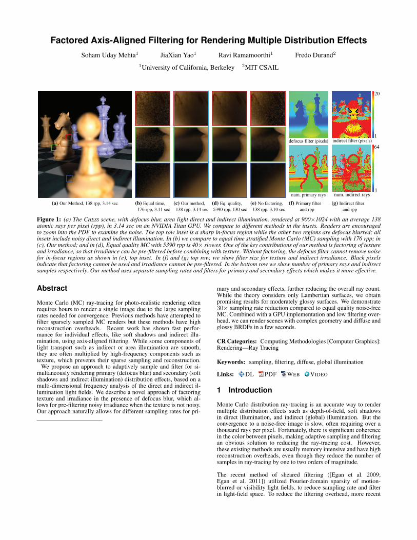
Figure 1: (a) The CHESS scene, with defocus blur, area light direct and indirect illumination, rendered at 900×1024 with an average 138atomic rays per pixel (rpp), in 3.14 sec on an NVIDIA Titan GPU. We compare to different methods in the insets. Readers are encouragedto zoom into the PDF to examine the noise. The top row inset is a sharp in-focus region while the other two regions are defocus blurred; allinsets include noisy direct and indirect illumination. In (b) we compare to equal time stratified Monte Carlo (MC) sampling with 176 rpp; in(c), Our method; and in (d), Equal quality MC with 5390 rpp is 40× slower. One of the key contributions of our method is factoring of textureand irradiance, so that irradiance can be pre-filtered before combining with texture. Without factoring, the defocus filter cannot remove noisefor in-focus regions as shown in (e), top inset. In (f) and (g) top row, we show filter size for texture and indirect irradiance. Black pixelsindicate that factoring cannot be used and irradiance cannot be pre-filtered. In the bottom row we show number of primary rays and indirectsamples respectively. Our method uses separate sampling rates and filters for primary and secondary effects which makes it more effective.

Abstract

Monte Carlo (MC) ray-tracing for photo-realistic rendering oftenrequires hours to render a single image due to the large samplingrates needed for convergence. Previous methods have attempted tofilter sparsely sampled MC renders but these methods have highreconstruction overheads. Recent work has shown fast perfor-mance for individual effects, like soft shadows and indirect illu-mination, using axis-aligned filtering. While some components oflight transport such as indirect or area illumination are smooth,they are often multiplied by high-frequency components such astexture, which prevents their sparse sampling and reconstruction.

We propose an approach to adaptively sample and filter for si-multaneously rendering primary (defocus blur) and secondary (softshadows and indirect illumination) distribution effects, based on amulti-dimensional frequency analysis of the direct and indirect il-lumination light fields. We describe a novel approach of factoringtexture and irradiance in the presence of defocus blur, which al-lows for pre-filtering noisy irradiance when the texture is not noisy.Our approach naturally allows for different sampling rates for pri-

mary and secondary effects, further reducing the overall ray count.While the theory considers only Lambertian surfaces, we obtainpromising results for moderately glossy surfaces. We demonstrate30× sampling rate reduction compared to equal quality noise-freeMC. Combined with a GPU implementation and low filtering over-head, we can render scenes with complex geometry and diffuse andglossy BRDFs in a few seconds.

CR Categories: Computing Methodologies [Computer Graphics]:Rendering—Ray Tracing

Keywords: sampling, filtering, diffuse, global illumination

Links: DL PDF WEB VIDEO

1 Introduction

Monte Carlo distribution ray-tracing is an accurate way to rendermultiple distribution effects such as depth-of-field, soft shadowsin direct illumination, and indirect (global) illumination. But theconvergence to a noise-free image is slow, often requiring over athousand rays per pixel. Fortunately, there is significant coherencein the color between pixels, making adaptive sampling and filteringan obvious solution to reducing the ray-tracing cost. However,these existing methods are usually memory intensive and have highreconstruction overheads, even though they reduce the number ofsamples in ray-tracing by one to two orders of magnitude.

The recent method of sheared filtering ([Egan et al. 2009;Egan et al. 2011]) utilized Fourier-domain sparsity of motion-blurred or visibility light fields, to reduce sampling rate and filterin light-field space. To reduce the filtering overhead, more recent

work on axis-aligned1 filtering ([Mehta et al. 2012; Mehta et al.2013]) for soft shadows and indirect illumination proposes amethod for adaptive sampling and image-space filtering that hasvery low overhead and makes fast render-times possible. But thesemethods are limited to rendering single effects rather than fulldistribution ray-tracing with multiple effects, and extending themto a higher-dimensional rendering domain is a challenge. Specif-ically, coupling between the irradiance and texture componentsof light transport (due to motion or defocus blur) hinders sparsesampling and reconstruction in proportion to the bandwidth of eachindividual component.

In this paper, we provide an axis-aligned method for image-space filtering that can handle a combination of different effects,namely defocus blur (primary), soft shadows and indirect illumi-nation (secondary). We do not consider motion blur in the mainpaper since our GPU ray-tracer doesn’t support it, but we providea proof-of-concept description with results, in the Appendix. Wederive a multi-dimensional end-to-end frequency analysis thathandles a combination of effects. Our analysis differs from pre-vious works in that it provides filtering bandwidths separately forboth the noisy texture and illumination using a simple geometricapproach. We introduce factoring of the radiance integral to moreefficiently sample and filter each component. Previous methodseither (i) filter the full high-dimensional light field [Lehtinen et al.2011; Lehtinen et al. 2012], resulting in large overhead, or (ii)use expensive atomic computation [Belcour et al. 2013] for eachray interaction to compute the overall bandwidth for the noisypixel color without factoring texture and irradiance. Our primarycontributions are:

Combined frequency analysis for primary and secondaryeffects: Our main theoretical contibution is the geometric andFourier analysis of both direct and indirect illumination underlens (defocus) blur for diffuse surfaces. We extend the flatland2D Fourier analysis of [Egan et al. 2011; Mehta et al. 2013],to the 3D light-field in a position-lens-light space for direct orposition-lens-angle space for indirect. We derive how the lightfield is bandlimited due to integration over the lens, light, andangle. Our approach is end-to-end unlike the atomic operationsof [Durand et al. 2005; Belcour et al. 2013]. This makes ourparameters easier to evaluate, without requiring complex frequencyanalysis along light paths.

Factoring texture and irradiance: Our main practical con-tribution is a method to approximate the integral of color (radiance)at each pixel as a product of texture and irradiance integrals. Inthe absence of defocus blur and spatial anti-aliasing, the primaryhit is a single location per-pixel, making factorization trivial, asassumed by previous irradiance filtering (e.g. irradiance caching)methods. However, due to defocus blur, the texture and irradianceare coupled. We propose to use the texture-irradiance factoringapproximation when the error is below a threshold. For example,an image region with a high-frequency texture (Fig. 1(e) top row)cannot be filtered without factorization, since we do not want toblur the texture. Hence, a large number of secondary rays wouldpreviously need to be traced to reduce the noise in soft shadowsand indirect illumination.

Two-level adaptive sampling strategy: Our method is basedsolely on ray-tracing for all rendering effects. Instead of naivelypath tracing each pixel, we allocate rays to primary and secondaryeffects in proportion to their frequency content while maintainingphysical correctness, as depicted in Fig.1(f,g) lower row. Forexample, at an in-focus pixel with soft shadows we allocate asingle lens ray but multiple light shadow rays. At an out-of-focuspixel with no soft shadows, we have an adequate number ofprimary rays, and a single shadow ray per primary ray. Similarly,we predict the sampling rate for indirect illumination taking

1Axis-aligned refers to the Fourier light-field rather than image-space,although the image-space filters as implemented are also axis-aligned.

into account both the local illumination frequency, and defocus.Previous adaptive sampling methods like [Belcour et al. 2013]only provide a single sampling rate at each pixel and hence areinefficient in reducing ray-tracing cost.

We have integrated our method into NVIDIA’s Optix ray-tracer [Parker 2010] and implemented our reconstruction methodon the GPU. We achieve about 4× ray count reduction comparedto equal RMS error MC (quantitative) and about 30× comparedto equal visual quality ground truth MC (qualitative). Figure 12emphasizes this point. Our method has a low reconstructionoverhead of under 200 ms, and can be easily combined with a GPUray-tracer. We demonstrate render times of 3-10 seconds2 for avariety of scenes.

2 Previous Work

[Cook et al. 1984] and [Kajiya 1986] first introduced Monte Carlodistribution ray and path tracing for evaluating pixel radianceusing the rendering equation. Building on the basic framework ofphysically based rendering, we use adaptive sampling and filteringto efficiently produce physically-based renderings with depth offield, and area light direct and indirect illumination.

Image Filtering and Noise-guided Reconstruction: Imagefiltering has been a popular approach to remove noise in imagesgenerated by MC ray-tracing, because of its simplicity andefficiency. Geometric information such as normals, textures, anddepths, can play an important role for predicting noise in renderedimages. Methods that use a denoising approach based on noiseestimation from geometric parameters include the use of the crossbilateral filter [Ritschel et al. 2009], the A-Trous wavelet transform[Dammertz et al. 2010], adaptive wavelet rendering [Overbecket al. 2009] and the filtering of stochastic buffers [Shirley et al.2011]. Other examples are random parameter filtering (RPF, [Senand Darabi 2012]) which has a high computation and storage cost,[Li et al. 2012] that uses Steins unbiased risk estimator for sam-pling and bandwidth selection for anisotropic filters, and [Rouselleet al. 2012] which uses non-local means filtering and residualerrors to guide sampling density. [Kalantari and Sen 2013] give anoise estimation metric to locally identify the amount of noise indifferent parts of the image, and adaptively sample and filter usingstandard denoising techniques. Another novel approach is that of[Sen et al. 2011] which uses compressed sensing. [Delbracio et al.2014] use ray color histograms to guide filtering. These methodsdo not exploit the geometric and Fourier structure of the lightfield and require either high sampling rates or high reconstructionoverheads. Our method is also different from 2D post-processingsolutions [Max and Lerner 1985; Potmesil and Chakravarty 1981]that blur a 2 or 2.5D image with spatially-varying filters accordingto depth or motion, since we filter an image obtained by accurateray and path tracing. Further, using a primary filter given by thecircle of confusion or motion vector does not filter noisy secondaryeffects.

Light Field Analysis: These methods attempt to reconstructthe full high-dimensional light field. Multi-dimensional adaptivesampling and reconstruction [Hachisuka et al. 2008] improvesupon [Mitchell 1991], and uses sample contrast to guide adaptivesampling, followed by anisotropic reconstruction of the lightfield. [Lehtinen et al. 2011] and [Lehtinen et al. 2012] proposeda reconstruction method for motion and defocus blur from sparsesampling of the 3D/5D (spatial position, lens and time) light fieldthat uses velocity and depth information to reproject samples intoeach pixel, but with a high memory and computation overhead.

Fourier-guided Adaptive Sampling and Filtering: We build onrecent approaches that have studied the frequency aspects of light

2We are slower than [Mehta et al. 2013] since we need more rays fordepth of field, and our images are at higher resolution.

Sample 1

Sampling

rate

Filter Widths

Texture

Irradiance

Radiance

Filter

Select Filter

Output

Sample 2

Figure 2: A simplified flow chart of the algorithm. In two sampling(ray-tracing) passes, we adaptively sample the noisy per-pixel tex-ture, irradiance and radiance. These are then filtered and combinedto produce an accurate radiance value.

transport in static scenes, e.g. [Chai et al. 2000; Ramamoorthi andHanrahan 2001; Durand et al. 2005]. They presented an a-priorifrequency analysis to perform adaptive sampling and appropriatereconstruction. [Egan et al. 2009; Egan et al. 2011] applied suchan analysis and sheared reconstruction to motion-blurred imagesand soft shadows utilizing the space-time and space-light Fourierspectra respectively. [Soler et al. 2009] proposed to adaptivelysample primary rays by predicting image bandwidth and per-pixelvariance of incoming light, to efficiently ray-trace and reconstructimages with depth of field. They used a sampled representation ofthe spectrum which is expensive and prone to noise. 5D covariancetracing [Belcour et al. 2013] uses a covariance representation thatis compact and stable, addressing the full 5D (space-angle-time)light field, and focuses on atomic operations to achieve generality.We instead use an image-space axis-aligned filter similar to [Mehtaet al. 2012; Mehta et al. 2013] combined with adaptive samplingfor both primary and secondary effects in a single framework.

Our method is simpler and faster than covariance tracing andgeneralizes axis-aligned filtering to combine primary and sec-ondary effects. Moreover, our texture-irradiance factorizationimproves on methods that only filter the final pixel radiance,without filtering irradiance. Those methods are inefficient forin-focus regions. Methods that retain the full light field (individualsamples) such as [Lehtinen et al. 2011; Lehtinen et al. 2012; Senand Darabi 2012] can filter the noisy irradiance separately buthave a high storage and reconstruction overhead. The concurrentwork of [Vaidyanathan et al. 2014] demonstrates a much faster,interactive formulation of sheared filtering for depth of field. Theyseparate the image into depth layers, and simplify the 4D filter intosplatting and screen-space convolution steps.

3 Overview

We describe our algorithm in brief to motivate the theoreticalanalysis and highlight the main contributions. A block diagram isshown in Fig 2. We first sparsely path trace each pixel to identifyfrequency bandwidths for each of the effects under consideration,namely the defocus blur, area light direct illumination and indirectillumination. Through this sparse sampling, we can predict thelocal Fourier structure of the high-dimensional light field for bothdirect and indirect illumination. Sections 4-6 derive this structureand corresponding reconstruction bandwidths.

For both the direct and indirect components at a pixel, weneed to decide if approximating the radiance integral by factoringinto a product of texture and irradiance integrals is possible. Know-ing the Fourier structure of the local light field gives us the requiredsampling rates for each component, as derived in Section 7. In asecond path-tracing pass, we trace the minimum adequate numberof primary rays to sample world location and texture, and then foreach primary ray, trace an appropriate number of secondary raysto compute the irradiance. Then, in the first filtering pass, if thefactorization was determined valid, we filter the factored direct andindirect irradiance. In a second filtering pass, we take the combined

Focal Plane

Surface

f

z

Lens

au

Sx/W

λΩx

Ωu

Ωx

Ωpix

d

max

rminΩu

max

r max

Figure 3: (a) Ray-tracing geometry for defocus blur. (b) Fourierspectrum and axis-aligned filter for defocus blur.

color at a pixel and apply the defocus filter. This gives the finalnoise free image. Implementation details are provided in Section 8.

Assumptions: The key assumption underlying our analysisis that surfaces are diffuse. Lambertian BRDFs allow a sim-ple end-to-end equation for multiple effects since there is noangle-dependence. However, our practical method works well formoderately glossy surfaces, and all of our results include glossydirect and indirect illumination. Note that we always filter samplesobtained by accurate ray or path tracing using the full BRDF. Wealso assume Gaussian lens aperture transmission and area lightintensity, like previous methods based on frequency analysis. Weevaluate the direct illumination form factor for a surface at thecenter of the light to simplify analysis and implementation, as inprevious work.

4 Defocus Blur

We now describe our Fourier light field analysis which guidesour bandwidth prediction. We first consider defocus blur only,assuming diffuse surfaces and a thin lens model. Secondaryeffects are discussed in the next two sections. Defocus blur is adistribution effect produced by primary (eye) rays, traced from thecamera lens of finite aperture out to the world focal plane.

Our derivation is in flatland, but the extension to the 3Dworld is straightforward. The set up is shown in Fig 3(a). Thescreen resolution is 2W , lens aperture is 2a and focal distance isf (in world space; we do not explicitly need to involve the focallength). Pixel coordinates x (pixel units) range in [−W,W ]; lenscoordinates u (dimensionless) range in [−1, 1]. A primary ray(x, u) is traced from world location (au, 0) to (Sx/W, f), where2S is the world space size (meters) of the focal plane. Consider aparallel surface at depth z from the lens, parametrized by λ, i.e. λis the world x-coordinate along the object. Then, the intersectionwith the object, of the primary ray (x, u) is

λ = au+z

f

(Sx

W− au

)=

Sz

Wf

(x+ auW

f − z

Sz

). (1)

Let us denote

r(x, u) =aW

S

(f

z(x, u)− 1

)(2)

as the width of the circle of confusion (in pixel units) for the rayhitpoint (x, u). We also define the magnification ℓp = (Sz/Wf)measured in meters per pixel, which transforms pixel-space x toworld space λ. For a non-parallel surface, r(x, u) changes for eachray, since the depth is not constant. Since the surface is pure diffuse,the light field at the camera sensor is

L(x, u) = Lo(λ) = Lo(ℓp · (x+ ru)). (3)

Here Lo(λ) is the intensity reflected by the receiver with argumentλ in meters. The Fourier transform of the light field is

L(Ωx,Ωu) =1

ℓpδ(Ωu − rΩx)Lo

(Ωx

ℓp

). (4)

All frequencies on the spatial axis are in pixel−1 units. Each par-allel receiver surface contributes a line in Fourier space (Ωx,Ωu),with slope given by its circle of confusion. Due to sloped or multi-ple receivers, the spectrum is a double wedge, as shown in Fig 3(b).The final color c at pixel x is

c(x) =∫L(x, u)A(u) du, (5)

where A(u) is the lens aperture function. The Fourier transform ofthe pixel-domain color is

c(Ωx) =∫L(Ωx,Ωu)A(−Ωu) dΩu. (6)

The lens aperture function bandlimits L(Ωx,Ωu), on the lens fre-quency axis, so that we can apply a simple filter to c as shown inFig 3(b). The spatial bandwidth of the axis-aligned filter is

Ωdx = min

Ωmax

pix , Ωmaxu /rmin

. (7)

Here Ωmaxpix = 0.5 is the maximum allowed pixel bandlimit (corre-

sponding to 1 sample per pixel) and Ωmaxu is the bandlimit of A(u).

This becomes an image-space filter implemented as a Gaussian withstd. deviation Ωd

x. We use the superscript d to denote defocus filterwidth, since we have different filters for different effects. We as-sume the lens to be a Gaussian with a 2σ width over u ∈ [−1, 1],so σ = 1, implying a standard deviation of σ = 1 in Fourier spaceand Ωmax

u = σ = 1. Since the primal-domain defocus filter widthRd

x (in pixels) is inversely proportial to the Fourier domain filterwidth, eqn. 7 implies:

Rdx = max 2, rmin . (8)

The minimum width of 2 pixels corresponds to the filter weightfor the adjacent pixel going to zero. As intuition would suggest,for diffuse surfaces, the defocus filter width is simply the smallestcircle of confusion at a pixel. The actual bandlimit can besomewhat smaller for glossy highlights, but the difference (fromusing a filter width derived for diffuse) is usually not noticeable.

Discussion: [Belcour et al. 2013] arrive at a similar resultfor the lens matrix that tranforms the light field’s covariancematrix. Although they are also able to handle glossy surfaces andocclusions in the same framework, their approach is also morecomplex and requires additional data structures for occlusion test-ing. [Soler et al. 2009] also give a light field analysis for defocusblur, using a series of atomic shears, and use the predicted shapeof the power spectrum to guide sampling and filtering. However,our approach is end-to-end unlike the approach of concatenatingatomic operators used in both [Belcour et al. 2013] and [Soleret al. 2009]. Neither of these papers explicitly equates the slopeof the defocused light field to the local circles of confusion. Theconcurrent work of [Vaidyanathan et al. 2014] does derive a verysimilar frequency analysis for defocus blur, but does not explorethe connections with direct and indirect illumination that we studynext.

5 Direct Illumination with defocus blur

While texture samples at a pixel are functions of the random lensposition alone, incident radiance samples (direct and indirect) arefunctions of two random parameters: the lens position and theillumination direction. Hence, reconstruction can be more efficientif the pixel irradiance can be pre-filtered to remove noise dueto incoming direction. To avoid the overhead of storing the full

Surface

u

x

y

Light

k(x,u)

(f.V)(x,u,y)

d1d2

(a)

Ωx

Ωy

Ωu

x

u y

(b)

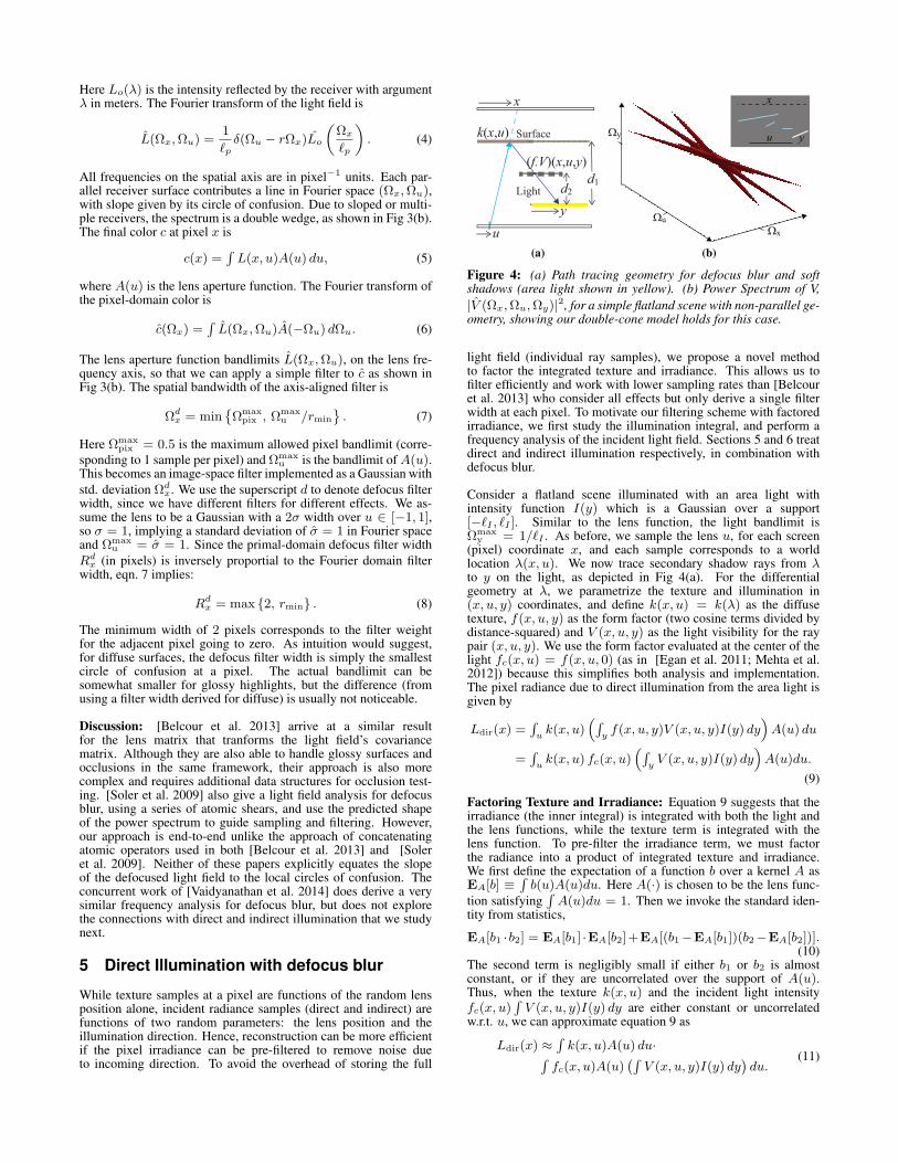
Figure 4: (a) Path tracing geometry for defocus blur and softshadows (area light shown in yellow). (b) Power Spectrum of V,|V (Ωx,Ωu,Ωy)|2, for a simple flatland scene with non-parallel ge-ometry, showing our double-cone model holds for this case.

light field (individual ray samples), we propose a novel methodto factor the integrated texture and irradiance. This allows us tofilter efficiently and work with lower sampling rates than [Belcouret al. 2013] who consider all effects but only derive a single filterwidth at each pixel. To motivate our filtering scheme with factoredirradiance, we first study the illumination integral, and perform afrequency analysis of the incident light field. Sections 5 and 6 treatdirect and indirect illumination respectively, in combination withdefocus blur.

Consider a flatland scene illuminated with an area light withintensity function I(y) which is a Gaussian over a support[−ℓI , ℓI ]. Similar to the lens function, the light bandlimit isΩmax

y = 1/ℓI . As before, we sample the lens u, for each screen(pixel) coordinate x, and each sample corresponds to a worldlocation λ(x, u). We now trace secondary shadow rays from λto y on the light, as depicted in Fig 4(a). For the differentialgeometry at λ, we parametrize the texture and illumination in(x, u, y) coordinates, and define k(x, u) = k(λ) as the diffusetexture, f(x, u, y) as the form factor (two cosine terms divided bydistance-squared) and V (x, u, y) as the light visibility for the raypair (x, u, y). We use the form factor evaluated at the center of thelight fc(x, u) = f(x, u, 0) (as in [Egan et al. 2011; Mehta et al.2012]) because this simplifies both analysis and implementation.The pixel radiance due to direct illumination from the area light isgiven by

Ldir(x) =∫uk(x, u)

(∫yf(x, u, y)V (x, u, y)I(y) dy

)A(u) du

=∫uk(x, u) fc(x, u)

(∫yV (x, u, y)I(y) dy

)A(u)du.

(9)

Factoring Texture and Irradiance: Equation 9 suggests that theirradiance (the inner integral) is integrated with both the light andthe lens functions, while the texture term is integrated with thelens function. To pre-filter the irradiance term, we must factorthe radiance into a product of integrated texture and irradiance.We first define the expectation of a function b over a kernel A asEA[b] ≡

∫b(u)A(u)du. Here A(·) is chosen to be the lens func-

tion satisfying∫A(u)du = 1. Then we invoke the standard iden-

tity from statistics,

EA[b1 ·b2] = EA[b1] ·EA[b2]+EA[(b1−EA[b1])(b2−EA[b2])].(10)

The second term is negligibly small if either b1 or b2 is almostconstant, or if they are uncorrelated over the support of A(u).Thus, when the texture k(x, u) and the incident light intensityfc(x, u)

∫V (x, u, y)I(y) dy are either constant or uncorrelated

w.r.t. u, we can approximate equation 9 as

Ldir(x) ≈∫k(x, u)A(u) du·∫

fc(x, u)A(u)(∫

V (x, u, y)I(y) dy)du.

(11)

We can rewrite this last approximation as

Ldir(x) ≈ kdir(x) · Edir(x), (12)

where we have defined the integrated texture term as

kdir(x) =∫k(x, u)A(u) du (13)

and the integrated irradiance term as

Edir(x) =∫fc(x, u)A(u)

(∫V (x, u, y)I(y) dy

)du. (14)

Almost all image-space global illumination methods ([Gershbeinet al. 1994; Ward and Heckbert 1992; Mehta et al. 2013], etc.)factor out the texture term and work with the irradiance. However,methods that deal with defocus blur cannot do this directly. If onlythe pixel radiance is filtered in image space (e.g. [Belcour et al.2013], [Li et al. 2012]), in a region with high frequency textureand small or no defocus, the shadow filter cannot be used (elsethe texture will be incorrectly blurred), and the light visibilitywill have to be sampled densely to remove noise. Our proposedfactorization allows us to pre-filter the irradiance term by the lightbandlimit separately, before multiplication by texture and applyingthe defocus blur filter. Without factoring, the pixel color frequencyis only determined by defocus blur magnitude, since the textureterm is not filtered by the light. To derive the filter and samplingrate for the irradiance, we perform a frequency analysis of thevisibility V (x, u, y).

Frequency analysis of light visibility in (x, u, y) space:We first perform a frequency analysis of the light visibility in(x, u, y) space, considering a parallel plane of occluders. Letg(·) be the one-dimensional visibility in the occluder plane. Theset up is as shown in Fig 4(a). Let ρ = d2/d1, where d1 and d2are distances of receiver and occluder from the light respectively.Then, the shadow light field on the receiver surface, following[Egan et al. 2011] and [Mehta et al. 2012], is3 g(ρλ + (1 − ρ)y).Hence, we have

V (x, u, y) = V (λ, y) = g(ρλ+ (1− ρ)y)

= g(ρℓp(x+ ru) + (1− ρ)y) ≡ g(αx+ βu+ γy). (15)

In the last step we have introduced the parameters α, β, γ to sim-plify the representation. Performing a 3D Fourier transform gives:

V (Ωx,Ωu,Ωy) =∫ ∫ ∫

g(αx+ βu+ γy)

exp(−j(xΩx + yΩy + uΩu))dx du dy

=1

αg

(Ωx

α

)δ

(Ωu − β

αΩx

)δ(Ωy − γ

αΩx

).

(16)

This is a line through the origin in 3D frequency space, normal tothe isosurface plane defined by eqn. 15. Due to the integration withaperture and light in eqn. 14, this line is bandlimited (clipped) bythe planes |Ωu| ≤ Ωmax

u and |Ωy| ≤ Ωmaxy . The two slopes given

by the delta functions in eqn. 16 imply that the line is clipped alongΩx to |Ωx| ≤ Ωmax

u /r and |Ωx| ≤ ℓpΩmaxy /(ρ−1 − 1). Let

s = ρ−1 − 1 = (d1/d2)− 1. (17)

s is analogous to r defined in eqn. 2. For non-parallel and multi-ple receivers and occluders, the visibility spectrum becomes a ban-dlimited double-cone in frequency space. As illustrated in Fig 4 (b)with a flatland simulation, this is a good approximation for arbitrar-ily oriented surfaces and area lights. The filter width (in per-pixel

3In general there will also be a constant offset in the argument of g(.)here, if the origins of the x and y coordinates are not aligned. However, theconstant offset does not affect the Fourier energy spectrum, so we ignore it.

units) that can be used to filter Edir according to the light bandlimitthen becomes

Ωsx = min

Ωmax

pix , ℓpΩmaxy /smin, Ω

maxu /rmin

(18)

Equivalently, the primal-domain filter size in pixels is

Rsx = max 2, ℓIsmin/ℓp, rmin . (19)

Filtering using factoring: In practice, we can use factoring(eqn. 12) wherever the error4 ||Ldir − kdir · Edir|| (obtained froma first sparse sampling pass) is small enough. For the pixels wherethe factorization is valid, we can filter Edir separately, by theshadow filter Ωs

x, then multiply by kdir and filter the product bythe defocus filter Ωd

x. Pre-filtering allows lower sampling rates forthe light visibility, thus saving on expensive ray-tracing. For pixelswhere the factorization is not valid, we filter the pixel radianceLdir(x) for defocus only. Usually these are pixels with a largedefocus width, and hence can gather radiance information frommany neighboring pixels, implying a lower sampling rate. Hence,most pixels can work with low sampling rates which are derived inSection 7.

In Fig 5(a) we show the pixel radiance Ldir from the firstsampling pass, and compare it to the integrated texture kdir in (b)and the integrated irradiance Edir in (c). The thresholded error isshown as a binary flag in (d). Object silhouettes or regions withhigh defocus blur cannot be factored, but those with soft shadowson smooth textures can. About 80% of pixels are separable for thisscene, but the fraction is larger for indirect illumination, and otherscenes. This makes our method much more efficient since we canpre-filter noisy irradiance.

(a) Ldir (b) kdir (c) Edir (d) SepDir

Figure 5: (a) The direct radiance Ldir for the CHESS scene from thefirst sampling pass (16 spp), (b) The factored texture kdir and (c)the separated irradiance Edir. (d) The factorization error||Ldir−kdir ·Edir|| is below a threshold except at the pixels markedblack (shown smoothed with a median filter).

Glossy Surfaces: Our filter widths Ωdx and Ωs

x are derivedassuming diffuse surfaces. Even though we do not handle glossysurfaces explicitly in our theory, our approximations work well forglossy direct and non-caustic indirect illumination, as demonstratedin our renders, all of which have glossy surfaces. This is becauseour filter is axis-aligned, and can capture a lot of energy that leaksbeyond the double-wedge model. We also filter an accuratelypath traced illumination for both diffuse and glossy components.To handle direct illumination on a glossy surface, suppose e isthe primary ray (x, u), and r is the direction from the hitpoint ofthe primary ray to the light’s center, reflected about the hitpointnormal. Then the Phong BRDF gloss factor evaluated at the lightcenter is simply (−e · r)m ≡ p(x, u). We can separate p(x, u) outinto the texture term. Explicitly, k(x, u) in eqn. 13 becomes

k(x, u) = kd(x, u) + ks(x, u)p(x, u) (20)

where kd and ks are the diffuse and specular textures respectively.

4|| · || is the standard euclidean distance between RGB colors.

6 Indirect Illumination

The total pixel radiance is the sum of the integrated direct andindirect radiance, i.e. L(x) = Ldir(x) + Lind(x), and we treatthe two components independently. Many of the same arguments,including factorization, that apply in the direct case, also apply toindirect illumination.

We use the parametrization in [Mehta et al. 2013], where in-cident radiance is a function of linearized direction v measured ina plane parallel to the local receiver. The indirect radiance Lind

at pixel x is the integral of the texture k(x, u), the BRDF andgeometry term5 h(v) and incoming indirect radiance li(x, u, v)reflected from the nearest surface in direction v. We can alsofactorize the texture and irradiance as follows:

Lind(x) =∫k(x, u)

(∫h(v)li(x, u, v) dv

)A(u)du

≈∫k(x, u)A(u) du ·

∫A(u)

(∫h(v)li(x, u, v) dv

)du

≡ kind(x) · Eind(x).(21)

This is similar to the direct lighting equation, with the lightintensity I replaced by the transfer function h. If the factorizationerror ||Lind − kind · Eind|| is small, we use the factored productkind · Eind. Factoring allows pre-filtering the Eind term andreducing the sampling rate required. If factoring is not possible,the radiance Lind can still be blurred by the defocus filter, and amoderate sampling rate suffices.

Assuming diffuse reflectors, the spectrum of the incident in-direct radiance li is also similar to that of the light visibility Vfrom the previous section. Extending the result of [Mehta et al.2013], individual reflectors contribute lines in the Fourier spacewith slope along the Ωx × Ωv plane given by the reflector depthz at (x, u, v). The slope along the Ωx × Ωu plane is given by thecircle of confusion r at (x, u). Similar to eqn. 18, the filter widthfor Eind is given by

Ωix = min

Ωmax

pix , ℓpΩmaxv /zmin, Ω

maxu /rmin

. (22)

Ωmaxv is the bandlimit of the low-pass transfer function h; the

numerical values for diffuse and glossy BRDFs can be foundin [Mehta et al. 2013]. The primal domain filter size is

Rix = max 2, zmin/(ℓpΩ

maxv ), rmin . (23)

Glossy Surfaces: The diffuse and glossy transfer functions h(v)are different (we need not know their exact forms), and the v de-pendence cannot be dropped to separate h from the Eind integral aswe did for f(x, u, y) in direct illumination. In other words, an ap-proximation like eqn. 20 cannot be made for indirect illumination.For the factorization kind · Eind to work for a surface with bothdiffuse and glossy components, each of Lind, kind, Eind must beevaluated and stored separately for the diffuse and glossy compo-nents. In the filtering pass, both diffuse and glossy Eind are filteredaccording to their own bandwidths given in equation 22 and thencombined with the appropriate kind.

7 Sampling Rates

Point sampling of the high-dimensional light field can cause alias-ing if the sampling rate is not sufficient, even if we subsequentlyuse the proper axis-aligned reconstruction filter. The minimumsampling rate is that which just prevents adjacent copies of spectrafrom overlapping our baseband filter. As in [Egan et al. 2009;

5The BRDF term is most generally a function of the world location also,i.e. h(x, u, v). We assume that the surface visible in a small neighborhoodaround a current pixel (for all u) is flat, and drop the x, u dependence.

Mehta et al. 2012; Mehta et al. 2013], we derive the minimumdistance between aliases of spectra, Ω∗

x,Ω∗u,Ω

∗y,Ω

∗v , and multiply

these to obtain the per-pixel sampling rates. However, the majordifference is that we derive different sampling rates for bothprimary and secondary rays. We allocate rays in proportion to thefrequency content of each effect, instead of using a fixed numberof secondary rays per primary ray at each pixel as has been done inprevious work.

In the first sampling pass, we trace a fixed number of raysper pixel to estimate bandwidths and sampling rates for the nextpass. In our main (second) sampling pass, at each pixel, we firstsend np primary rays from the lens, then for direct illuminationwe trace a number of shadow rays for each of these np primaryrays so that the total number is ndir. For indirect illumination, foreach primary ray a certain number of indirect radiance samplesare obtained, so that the total number is nind. In addition, oursecondary sampling rates vary depending on whether we use theexact radiance, or factored texture and irradiance. Superscripts ‘c’(combined) and ‘f’ (factored) are used to denote these two differentsecondary sampling rates respectively.

For determining the primary sampling rate, we need onlyconsider simple defocus blur (assuming diffuse surfaces). Ouraxis-aligned filter was described in Section 4. The minimumprimary sampling rate is obtained considering aliasing in Ωx ×Ωu

space, as shown in Fig. 6(a). We have,

np = (Ω∗x)

2(Ω∗u)

2

= (Ωmaxpix +Ωd

x)2(1 + rmaxΩ

dx)

2.

(24)

Although [Soler et al. 2009] use power spectral energy and varianceto determine their sampling rate, their overall sampling density indefocused regions looks similar to ours. However, their samplingmethod is quite different as they obtain image and lens samples inFourier space.

Ωx

*Ωx

*Ωu

Ωpixd max

Ωumax

rmaxΩxd

Ωx

Ωu

Ωx

Ωpixmax

Ωymax

Ωxs

Ωy

Ωumax

Ωu

Figure 6: (a) Packing of aliases for defocus only, showing the spa-tial and lens sampling rates Ω∗

x and Ω∗u (b) Packing for aliases of

the light visibility V . The yellow and grey double wedges are theprojection on the Ωx×Ωy and Ωx×Ωu planes respectively. Aliasesnot shown for clarity. The minimum sampling rates Ω∗

x,Ω∗y and Ω∗

u

are analogous to those shown in (a).

Secondary sampling rate with factored texture and irradiance:For area light direct illumination, the visibility in equation (7) mustbe sampled sufficiently to avoid aliasing in each of the (x, u, y) di-mensions. At pixels with factored direct illumination, filtering Edir

clips it to a spatial Fourier width of Ωsx. This case is illustrated

in Figure 6(b), with projections of the spectrum on two coordinateplanes instead of the full volumetric spectrum for clarity. The min-imum separation for no aliasing along each axis follows similarlyfrom the 2D packing for defocus only; the per-pixel sampling rate

for V (x, u, y) (secondary shadow rays) is

nfdir = (Ω∗

x)2(Ω∗

u)2(Ω∗

y)2ℓ2I

= (Ωmaxpix +Ωs

x)2(1 + rmaxΩ

sx)

2(1 + ℓIsmaxΩsx/ℓp)

2

(25)

Similarly, for indirect illumination the indirect light field li in equa-tion (12) must be sampled more to avoid aliasing in each of the(x, u, v) dimensions. When factored irradiance is used, the spec-trum is clipped to a bandlimit Ωi

x. The sampling rate is then,

nfind = (Ω∗

x)2(Ω∗

u)2(Ω∗

v)2

= (Ωmaxpix +Ωi

x)2(1 + rmaxΩ

ix)

2(Ωmaxv + zmaxΩ

ix/ℓp)

2

(26)

Secondary sampling rate without factoring: If the direct radi-ance cannot be factored into texture and irradiance, only the defo-cus filter must be applied to the radiance. The light field spectrumis then clipped to a bandlimit Ωd

x. The direct illumination samplingrate is then

ncdir = (Ωmax

pix +Ωdx)

2(1 + rmaxΩdx)

2(1 + ℓIsmaxΩdx/ℓp)

2 (27)

Finally, without factorization, the indirect illumination samplingrate is

ncind = (Ωmax

pix +Ωdx)

2(1+rmaxΩdx)

2(Ωmaxv +zmaxΩ

dx/ℓp)

2 (28)

Discussion: Observe from eqns. 7, 18 that Ωsx ≤ Ωd

x ≤ Ωmaxpix . As

expected, if the pixel is in focus (i.e., either f = z or a = 0) thenumber of primary rays per pixel is np = (2Ωmax

pix )2 = 1 sincermax = rmin = 0. Similarly, nc

dir = np if we have a point lightwith ℓI = 0. This means we only take one visibility sample ifthe light size shrinks to zero, verifying that our formulae work inthe limit. Further, observe that nf

dir ≤ ncdir, since the former uses

a smaller spatial bandlimit. This is expected, since the ability tofilter the irradiance Edir allows for a lower secondary samplingrate. Also note that at a pixel that uses factored irradiance, thedefocus is typically small, and then nf

dir ≥ np since the secondarysampling rate has an extra (Ω∗

y)2 term in eqn. 25. Then we must

trace nfdir/np ≥ 1 secondary rays per primary ray6.

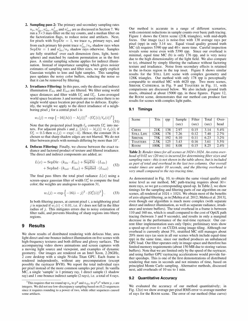
We now qualitatively discuss our practical sampling ratesshown in fig 8(e)-(g). First, in the region marked ‘A’, we havea high defocus and depth variance, and hence we provide morerays for all effects (i.e. np, ndir, nind are all large, but this type ofregion covers only a small part of the image). In the region marked‘B’, which is in-focus, we need few primary rays but many indirectsamples since it has nearby reflectors. In ‘C’, the wall is defocusedbut at a constant depth, so a few primary rays suffice, but moredirect and indirect samples are needed.

Convergence with increasing sampling rate: As in [Mehtaet al. 2012; Mehta et al. 2013] we can control our samplingrates with a user-defined parameter µ. To implement this, eachreconstruction bandwidth is simply scaled by µ and the samplingrates are then computed as above. For example, the primarysampling rate as a function of µ becomes:

np(µ) = (Ωmaxpix +Ωd

x(µ))2(1 + rmaxΩ

dx(µ))

2, (29)

where Ωdx(µ) = min

Ωmax

pix , µ · Ωdx

. Thus, we can smoothly con-

trol our speed and accuracy, and converge to ground truth with in-creasing ray count. We demonstrate this quantitatively as an error-vs-rpp plot in Fig. 12(e). Controlling sampling rate and filter size

6However, a pixel with constant texture and high defocus can also allowfactorization. In this and some other cases, we may also have nf

dir < np,but for physical correctness we trace one secondary ray per primary ray.

using µ can also be used to speed-up our method by starting withlow µ and updating the image with increasing µ, and refreshingif the camera or light is changed. We demonstrate this interactivepre-view rendering system in our video.

8 Implementation

A flow chart of our algorithm is shown in Figure 7. All quantitiesare concisely defined in Table 1 which also points to the relevantequations.

Sampling

Pass 1

Secondary

Filter Primary

Filter

Sampling

Pass 2

Figure 7: Flow chart of the algorithm for the direct componentonly; the indirect component is handled similarly. Filled blocks arevariables stored in memory, empty blocks are operations. Refer totable 1 for definitions of variables.

Quantity Description Equation

Ldir integrated color, direct component 9kdir integrated texture, direct component 13Edir integrated illumination, direct component 14Lind integrated color, indirect component 21kind integrated texture, indirect component 21Eind integrated illumination, indirect component 21

SepDir Boolean, set if direct factorization error is small 30SepInd Boolean, set if indirect factorization error is small 30

rmin, rmax min, max circle of confusion in pixels 2smin, smax min, max soft shadow slopes 17zmin, zmax min, max reflector distance for indirect -

Ωdx depth-of-field filter width 7

Ωsx direct illumination filter width 16

Ωix indirect illumination filter width 19

np Num. primary (lens) rays 24ncdir Num. light shadow rays if SepDir = 0 27

nfdir Num. light shadow rays if SepDir = 1 25

ncind Num. indirect samples if SepInd = 0 28

nfind Num. indirect samples if SepInd = 1 26

Table 1: A list of the variables we store in a per-pixel buffer. Thedefining equation for each variable is indicated in the last column.

Our algorithm is implemented in multiple consecutive pixel shaderpasses in NVIDIA’s Optix ray-tracer. The source code will be madeavailable online upon publication.

1. Sampling pass 1: We first trace 16 paths per pixel into thescene. A single path is one primary lens ray, one secondaryshadow ray, and a one-bounce indirect sample (separate fordiffuse and glossy). We draw lens samples, light samples (fordirect) and hemisphere samples (for indirect) from a 4 × 4stratification each, and match the samples with random per-mutations [Shirley and Morley 2003]. At each pixel we accu-mulate the colors Ldir, kdir, Edir, Lind, kind, Eind. The directparameters smin, smax, indirect parameters zmin, zmax anddefocus parameters cmin, cmax, and the lens-averaged worldlocation, projected area Ap, and normal are computed. Fromthese we compute the filter widths Ωr

x,Ωsx,Ω

ix and set flags:

SepDir = ||Ldir − kdir · Edir|| < 0.01

SepInd = ||Lind − kind · Eind|| < 0.01 (30)

2. Sampling pass 2: The primary and secondary sampling ratesnp, n

fdir, n

cdir, n

find and nc

ind are as discussed in Section 7. Werun a 3×3 max-filter on the ray counts, and a median filter onthe factorization flags, to reduce noise and artifacts. Next,for pixels with SepDir = 1, we trace np primary rays, andfrom each primary hit-point trace nf

dir/np shadow rays whenSepDir = 1 and nc

dir/np shadow rays otherwise. Samplesare fully stratified7 over each dimension (lens, light, hemi-sphere) and matched by random permutation as in the firstpass. A similar sampling scheme applies for indirect illumi-nation. Instead of importance sampling which gives noisierestimates of sampling rates and filter sizes, we apply explicitGaussian weights to lens and light samples. This samplingpass updates the noisy color buffers, reducing the noise sothat it can be removed by filtering.

3. Irradiance Filtering: In this pass, only the direct and indirectillumination Edir and Eind are filtered. We filter using worldspace distances and filter width Ωs

x and Ωix. Lens-averaged

world space locations λ and normals are used since there is nosingle world space location per-pixel due to defocus. Explic-itly, the weight we apply to the direct irradiance of a neigh-boring pixel j for a central pixel i is

wi(j) = exp−16||λ(i)− λ(j)||2 · (Ωs

x(i)/ℓp(i))2

(31)Note that the projected pixel length ℓp converts Ωs

x into me-ters. For adjacent pixels i and j, ||λ(i) − λ(j)|| ≈ ℓp(i); ifΩs

x = 0.5 then wi(j) = exp(−4). Hence, the constant 16 ischosen so that sharp shadow edges are not blurred. We do notfilter between pixels with normals differing by more than 10.

4. Defocus Filtering: Finally, we choose between the exact ra-diance and factored product of texture and filtered irradiance.The direct and indirect components are added, as:

L(x) = SepDir · (kdir · Edir) + SepDir · (Ldir)

+ SepInd · (kind · Eind) + SepInd · (Lind)(32)

The final pass filters the total pixel radiance L(x) using ascreen-space gaussian filter of width Ωd

x to compute the finalcolor; the weights are analogous to equation 31,

wi(j) = exp−16(i− j)2 · (Ωd

x(i))2. (33)

In both filtering passes, at current pixel i, a neighboring pixelj is rejected if wj(i) < 0.01, i.e. if i does not fall in the filterradius of j. This mitigates errors due to noisy estimation offilter radii, and prevents bleeding of sharp regions into blurryregions.

9 Results

We show results of distributed rendering with defocus blur, arealight direct and one-bounce indirect illumination on five scenes withhigh-frequency textures and both diffuse and glossy surfaces. Theaccompanying video shows animations and screen captures witha moving light source and viewpoint, and examples of dynamicgeometry. Our images are rendered on an Intel Xeon, 2.26GHz,2 core desktop with a single Nvidia Titan GPU. Each frame isrendered independently, without any precomputation (exceptpossibly the raytracer BVH). We report the total individual raysper pixel instead of the more common samples per pixel. In vanillaMC, a single ‘sample’ is 1 primary ray, 1 direct sample (1 shadowray) and 1 one-bounce indirect sample (2 rays), i.e. a total of 4 rays.

7This requires that we round up np to p2 and ndir to p2s2 where p, s areintegers. We did not use low-discrepancy sampling based on (0,2) sequencessince it requires rounding to a power of two, while other sequences causedsome artifacts.

Our method is accurate in a range of different scenarios,with consistent reductions in sample counts over basic path tracing.Figure 1 shows the CHESS scene (21K triangles), with mid-depthfocus. Our image (a,c) is noise-free with 138 average rays perpixel (rpp) in only 3.14 sec. Equal visual quality ground truthMC (d) requires 5390 rpp and 40× more time. Careful inspectionreveals some noise even with 5390 rpp. Since our overhead isminimal, equal time MC (b) is only 176 rpp, and is very noisydue to the high dimensionality of the light field. We also compareto (e), obtained by simply filtering the radiance without factoringtexture and irradiance. Noise from secondary effects is retainedin the in-focus region in the top inset. Figure 8 shows similarresults for the STILL LIFE scene with complex geometry and128K triangles. Our method with only 178 rpp is perceptuallycomparable to stratified MC with 4620 rpp. Two more scenes,SIBENIK CATHEDRAL in Fig. 9 and TOASTERS in Fig. 11, withcomparisons are discussed below. We also include ground truthinsets, obtained at about 15000 rpp, in these figures. Figure 12,the ROOM scene, demonstrates that our method can produce fastresults for scenes with complex light paths.

9.1 Timings

Scene Tris rpp Sample Filter Total Over-(sec) (sec) (sec) head

CHESS 21K 138 2.97 0.15 3.14 5.4%STILL LIFE 128K 178 7.26 0.12 7.40 2.7%SIBENIK 75K 192 6.10 0.11 6.23 3.2%TOASTERS 2.5K 125 3.43 0.16 3.61 5.5%ROOM 100K 181 8.08 0.15 8.25 2.4%

Table 2: Render times for all scenes at 1024×1024. An extra over-head of 0.02 sec (20 ms) is incurred for determining filter sizes andsampling rates - this is not shown in the table above, but is includedas part of total and overhead in the last two columns. Our overallrender times are under 10 seconds, and the filtering overhead isvery small compared to the ray-tracing time.

As demonstrated in Fig. 10, to obtain the same visual quality andnoise level as our method, MC path-tracing requires about 30×more rays, so we get a corresponding speed-up. In Table 2, we showtimings for the sampling and filtering parts of our algorithm on ourscenes, all rendered at 1024×1024. We obtain most of the benefitsof axis-aligned filtering, as in [Mehta et al. 2012; Mehta et al. 2013],even though our algorithm is much more complex (with separatedirect and indirect illumination, as well as separate radiance, irradi-ance and texture buffers). The total overhead in a frame is between110 and 160 ms, which is small compared to the cost of OptiX pathtracing (between 3 and 9 seconds), and results in only a marginaldecrease in the performance of the real-time raytracer. Our cur-rent filter implementation uses only Optix; preliminary tests showa speed-up of over 4× on CUDA using image tiling. Although ouroverhead is currently about 5%, stratified MC still manages about20% more rays (as seen in all our scenes which include equal-timerpp) in the same time, since our method produces an unbalancedGPU load. Our filter operates only in image-space and therefore haslimited memory requirements (about 150 MB due to storing variousbuffers). Note that we are limited only by the speed of the raytracer,and using further GPU raytracing accelerations would provide fur-ther speedups. This is one of the first demonstrations of distributedrendering that runs in seconds and not minutes of time, based onprincipled Monte Carlo sampling. Alternative methods, discussednext, add overheads of 10 sec to 1 min.

9.2 Quantitative Accuracy

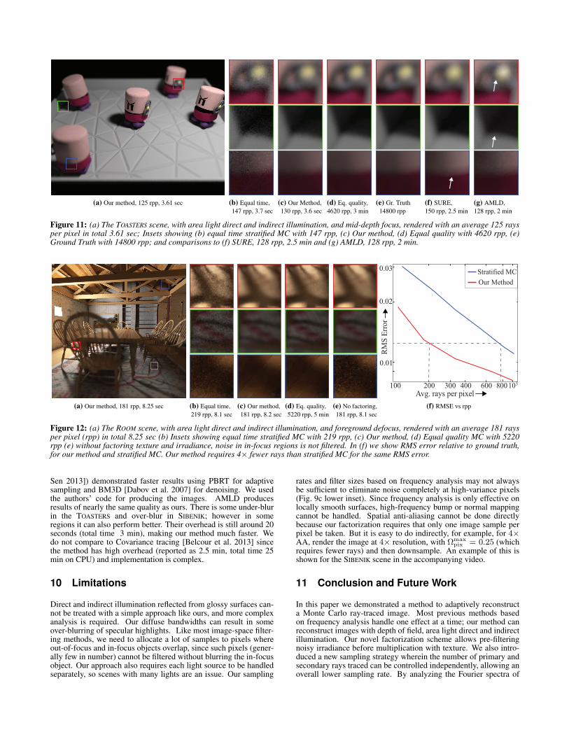
We evaluated the accuracy of our method quantitatively; inFig. 12(e) we show average per-pixel RMS error vs average numberof rays for the ROOM scene. The error of our method (blue curve)

(a) Our method, 178 rpp, 7.40 sec (b) Equal time,220 rpp, 7.4 sec

(c) Our method,178 rpp, 7.4 sec

(d) Eq. quality,4620 rpp, 4.5 min

Rx in pixelsd

primary rays (np)

A C

B

A C

B

(e) Primary rppand filter

Rx in pixelss

shadow rays (ndir)

A C

B

A C

B

(f) Direct rppand filter

1

20

1

64Rx in pixelsi

indirect rays (nind)

A C

B

A C

B

(g) Indirect sppand filter

Figure 8: The STILL LIFE scene, with defocus blur, area light direct and indirect illumination, rendered in 7.40 sec with an average 178 raysper pixel (rpp). The insets compare (b) equal time stratified MC, (c) our method, and (d) equal quality stratified MC with 4620 rpp (275 sec).In (e)-(g), we show heatmaps for our three filter widths and sampling rates, namely for defocus, and direct and indirect illumination. A moredetailed discussion is provided near the end of Sec. 7.

(a) Our method, 192 rpp, 6.23 sec (b) Equal time,229 rpp, 6.3 sec

(c) Our Method,192 rpp, 6.2 sec

(d) Eq. quality,5400 rpp, 3.5 min

(e) Gr. Truth,16400 rpp

(f) SURE,200 rpp, 4 min

(g) AMLD,200 rpp, 4 min

Figure 9: (a) The SIBENIK CATHEDRAL scene, with area light direct and indirect illumination, and foreground defocus, with an average 192rays per pixel (rpp) requires 6.23 sec; and insets showing (b) equal time stratified MC with 229 rpp, (c) Our method, (d) Equal quality with5400 rpp and (e) Ground truth with 16400 rpp. We also compare to (f) SURE, with 200 rpp rendered in 4 min and (g) AMLD with 200 rpp in4 min.

is significantly below stratified Monte Carlo at all sample counts,and for the same error we require about 4× less rays. As we in-crease the number of rays (higher µ, eqn. 29), we do converge toground truth and error decreases. This is in contrast to most previ-ous solutions for filtering MC images which do not provide a simplesolution to converge with increasing ray count. Since our methodreplaces some of the noise with some bias, equal perceptual error isachieved at over 30× fewer ray counts, as illustrated in Fig. 10.

9.3 Comparisons

We have already discussed comparison to brute-force equal timeand equal visual quality MC. In Figs. 9(f,g) and 11(f,g), weinclude comparison insets to two alternative recent approaches toMC denoising. Insets of the other methods use a similar averagenumber of rays.

We compare to SURE, [Li et al. 2012], since for the samequality, they are faster than other recent approaches such as [Senand Darabi 2012; Rousselle et al. 2011], etc. The comparison

MC, 3500 rpp MC, 5220 rpp MC, 7000 rppOur, 180 rpp

Figure 10: We compare stratified MC and our method with increas-ing sample count for an inset from the ROOM scene (Fig. 12). Strat-ified MC visually matches our method for about 5220 rpp. At 180rpp, our method is very slightly over-blurred, but MC at 5220 rppshows more noise (zoom in) in comparison.

insets show that SURE slightly over-blurs both in-focus andout-of-focus regions if the original image is very noisy. Theauthors’ implementation with PBRT requires around 4 min, witha filtering overhead of 1 min due to its multiple filtering passes.It also requires a slightly higher sampling rate for the samequality. Adaptive Multi-Level Denoising (AMLD, [Kalantari and

(a) Our method, 125 rpp, 3.61 sec (b) Equal time,147 rpp, 3.7 sec

(c) Our Method,130 rpp, 3.6 sec

(d) Eq. quality,4620 rpp, 3 min

(e) Gr. Truth14800 rpp

(f) SURE,150 rpp, 2.5 min

(g) AMLD,128 rpp, 2 min

Figure 11: (a) The TOASTERS scene, with area light direct and indirect illumination, and mid-depth focus, rendered with an average 125 raysper pixel in total 3.61 sec; Insets showing (b) equal time stratified MC with 147 rpp, (c) Our method, (d) Equal quality with 4620 rpp, (e)Ground Truth with 14800 rpp; and comparisons to (f) SURE, 128 rpp, 2.5 min and (g) AMLD, 128 rpp, 2 min.

(a) Our method, 181 rpp, 8.25 sec (b) Equal time,219 rpp, 8.1 sec

(c) Our method,181 rpp, 8.2 sec

(d) Eq. quality,5220 rpp, 5 min

(e) No factoring,181 rpp, 8.1 sec

100 200 300 400 600 103

0.01

0.02

0.03Stratified MC

Our Method

800Avg. rays per pixel

RM

S E

rror

(f) RMSE vs rpp

Figure 12: (a) The ROOM scene, with area light direct and indirect illumination, and foreground defocus, rendered with an average 181 raysper pixel (rpp) in total 8.25 sec (b) Insets showing equal time stratified MC with 219 rpp, (c) Our method, (d) Equal quality MC with 5220rpp (e) without factoring texture and irradiance, noise in in-focus regions is not filtered. In (f) we show RMS error relative to ground truth,for our method and stratified MC. Our method requires 4× fewer rays than stratified MC for the same RMS error.

Sen 2013]) demonstrated faster results using PBRT for adaptivesampling and BM3D [Dabov et al. 2007] for denoising. We usedthe authors’ code for producing the images. AMLD producesresults of nearly the same quality as ours. There is some under-blurin the TOASTERS and over-blur in SIBENIK; however in someregions it can also perform better. Their overhead is still around 20seconds (total time 3 min), making our method much faster. Wedo not compare to Covariance tracing [Belcour et al. 2013] sincethe method has high overhead (reported as 2.5 min, total time 25min on CPU) and implementation is complex.

10 Limitations

Direct and indirect illumination reflected from glossy surfaces can-not be treated with a simple approach like ours, and more complexanalysis is required. Our diffuse bandwidths can result in someover-blurring of specular highlights. Like most image-space filter-ing methods, we need to allocate a lot of samples to pixels whereout-of-focus and in-focus objects overlap, since such pixels (gener-ally few in number) cannot be filtered without blurring the in-focusobject. Our approach also requires each light source to be handledseparately, so scenes with many lights are an issue. Our sampling

rates and filter sizes based on frequency analysis may not alwaysbe sufficient to eliminate noise completely at high-variance pixels(Fig. 9c lower inset). Since frequency analysis is only effective onlocally smooth surfaces, high-frequency bump or normal mappingcannot be handled. Spatial anti-aliasing cannot be done directlybecause our factorization requires that only one image sample perpixel be taken. But it is easy to do indirectly, for example, for 4×AA, render the image at 4× resolution, with Ωmax

pix = 0.25 (whichrequires fewer rays) and then downsample. An example of this isshown for the SIBENIK scene in the accompanying video.

11 Conclusion and Future Work

In this paper we demonstrated a method to adaptively reconstructa Monte Carlo ray-traced image. Most previous methods basedon frequency analysis handle one effect at a time; our method canreconstruct images with depth of field, area light direct and indirectillumination. Our novel factorization scheme allows pre-filteringnoisy irradiance before multiplication with texture. We also intro-duced a new sampling strategy wherein the number of primary andsecondary rays traced can be controlled independently, allowing anoverall lower sampling rate. By analyzing the Fourier spectra of

the direct and indirect illumination light fields, we derived imagespace bandlimits for both the radiance and irradiance. Our rendertimes are around 5 seconds, and our overhead is more than 50×lower than state-of-the-art.

It could also be possible to combine our approach with amany-lights framework [Walter et al. 2006] to handle more generallighting environments. Finally, it would also be interesting to seeif the approach can be extended for noisy caustics from highlyspecular surfaces.

12 Acknowledgements

We thank the reviewers for their helpful suggestions. This workwas supported in part by NSF grant CGV #1115242, 1116303, andthe Intel Science and Technology Center for Visual Computing. Wethank NVIDIA for graphics cards, and fellowship support.

References

BELCOUR, L., SOLER, C., SUBR, K., HOLZSCHUCH, N.,AND DURAND, F. 2013. 5D covariance tracing for efficientdefocus and motion blur. ACM Transanctions on Graphics32, 3, 31:1–31:18.

CHAI, J.-X., TONG, X., CHAN, S.-C., AND SHUM, H.-Y.2000. Plenoptic Sampling. In Proceedings of SIGGRAPH 00,307–318.

COOK, R., PORTER, T., AND CARPENTER, L. 1984. Dis-tributed Ray Tracing. In Proceedings of SIGGRAPH 84, 137–145.

DABOV, K., FOI, A., KATKOVNIK, V., AND EGIAZARIAN,K. 2007. Image denoising by sparse 3D transform-domain col-laborative filtering. IEEE Transactions on Image Processing16, 8, 2080–2095.

DAMMERTZ, H., SEWTZ, D., HANIKA, J., AND LENSCH,H. P. A. 2010. Edge-avoiding A-trous wavelet transform forfast global illumination filtering. In Proceedings of the Con-ference on High Performance Graphics, 67–75.

DELBRACIO, M., MUSE, P., BUADES, A., CHAUVIER, J.,PHELPS, N., AND MOREL, J.-M. 2014. Boosting montecarlo rendering by ray histogram fusion. ACM Transactionson Graphics 33, 1, 8:1–8:15.

DURAND, F., HOLZSCHUCH, N., SOLER, C., CHAN, E.,AND SILLION, F. 2005. A Frequency Analysis of Light Trans-port. ACM Transactions on Graphics 24, 3, 1115–1126.

EGAN, K., TSENG, Y., HOLZSCHUCH, N., DURAND, F.,AND RAMAMOORTHI, R. 2009. Frequency analysis andsheared reconstruction for rendering motion blur. ACM Trans-actions on Graphics 28, 3, 93:1–93:13.

EGAN, K., HECHT, F., DURAND, F., AND RAMAMOOR-THI, R. 2011. Frequency analysis and sheared filtering forshadow light fields of complex occluders. ACM Transactionson Graphics 30, 2, 9:1–9:13.

GERSHBEIN, R., SCHRODER, P., AND HANRAHAN, P. 1994.Textures and Radiosity: Controlling Emission and Reflectionwith Texture Maps. In Proceedings of SIGGRAPH 94, 51–58.

HACHISUKA, T., JAROSZ, W., WEISTROFFER, R., DALE,K., HUMPHREYS, G., ZWICKER, M., AND JENSEN, H.2008. Multidimensional adaptive sampling and reconstructionfor ray tracing. ACM Transactions on Graphics 27, 3, 33:1–33:10.

KAJIYA, J. 1986. The Rendering Equation. In Proceedings ofSIGGRAPH 86, 143–150.

KALANTARI, N. K., AND SEN, P. 2013. Removing the noise inMonte Carlo rendering with general image denoising algorithms.Computer Graphics Forum (Proc. of Eurographics 2013)32, 2, 93–102.

LEHTINEN, J., AILA, T., CHEN, J., LAINE, S., AND DU-RAND, F. 2011. Temporal light field reconstruction for render-ing distribution effects. ACM Transactions on Graphics 30,4, 55:1–55:12.

LEHTINEN, J., AILA, T., LAINE, S., AND DURAND, F. 2012.Reconstructing the indirect light field for global illumination.ACM Transanctions on Graphics 31, 4, 51:1–51:10.

LI, T.-M., WU, Y.-T., AND CHUANG, Y.-Y. 2012. SURE-based optimization for adaptive sampling and reconstruction.ACM Transactions on Graphics 31, 6, 186:1–186:9.

MAX, N. L., AND LERNER, D. M. 1985. A two-and-a-half-D motion-blur algorithm. In Proceedings of SIGGRAPH 85,85–93.

MEHTA, S., WANG, B., AND RAMAMOORTHI, R. 2012.Axis-aligned filtering for interactive sampled soft shadows.ACM Transactions on Graphics 31, 6, 163:1–163:10.

MEHTA, S. U., WANG, B., RAMAMOORTHI, R., ANDDURAND, F. 2013. Axis-aligned filtering for interactivephysically-based diffuse indirect lighting. ACM Transactionson Graphics 32, 4, 96:1–96:12.

MITCHELL, D. 1991. Spectrally Optimal Sampling for Distribu-tion Ray Tracing. In SIGGRAPH 91, 157–164.

OVERBECK, R., DONNER, C., AND RAMAMOORTHI, R.2009. Adaptive Wavelet Rendering. ACM Transactions onGraphics 28, 5.

POTMESIL, M., AND CHAKRAVARTY, I. 1981. A lens andaperture camera model for synthetic image generation. In Pro-ceedings of SIGGRAPH 81, 297–305.

RAMAMOORTHI, R., AND HANRAHAN, P. 2001. A Signal-Processing Framework for Inverse Rendering. In Proceedingsof SIGGRAPH 01, 117–128.

RITSCHEL, T., ENGELHARDT, T., GROSCH, T., SEIDEL,H.-P., KAUTZ, J., AND DACHSBACHER, C. 2009. Micro-rendering for scalable, parallel final gathering. ACM Transac-tions on Graphics 28, 5, 132:1–132:8.

ROUSELLE, F., KNAUS, C., AND ZWICKER, M. 2012. Adap-tive rendering with non-local means filtering. ACM Transac-tions on Graphics 31, 6, 195:1–195:11.

ROUSSELLE, F., KNAUS, C., AND ZWICKER, M. 2011.Adaptive sampling and reconstruction using greedy error min-imization. ACM Transactions on Graphics 30, 6, 159:1–159:12.

SEN, P., AND DARABI, S. 2012. On filtering the noise from therandom parameters in monte carlo rendering. ACM Transac-tions on Graphics 31, 3, 18:1–18:15.

SEN, P., DARABI, S., AND XIAO, L. 2011. Compressive ren-dering of multidimensional scenes. In Proceedings of the 2010International Conference on Video Processing and Compu-tational Video, Springer-Verlag, Berlin, Heidelberg, 152–183.

SHIRLEY, P., AND MORLEY, R. K. 2003. Realistic Ray Trac-ing, 2 ed. A. K. Peters, Ltd., Natick, MA, USA.

SHIRLEY, P., AILA, T., COHEN, J., ENDERTON, E., LAINE,S., LUEBKE, D., AND MCGUIRE, M. 2011. A local im-age reconstruction algorithm for stochastic rendering. In ACMSymposium on Interactive 3D Graphics, 9–14.

SOLER, C., SUBR, K., DURAND, F., HOLZSCHUCH, N.,AND SILLION, F. 2009. Fourier depth of field. ACM Trans-actions on Graphics 28, 2, 18:1–18:12.

VAIDYANATHAN, K., MUNKBERG, J., CLARBERG, P., ANDSALVI, M. 2014. Layered Light Field Reconstruction forDefocus Blur. To appear in ACM Transactions on Graph-ics. http://software.intel.com/en-us/articles/layered-light-field-reconstruction-for-defocus-blur.

WALTER, B., ARBREE, A., BALA, K., AND GREENBERG,D. 2006. Multidimensional lightcuts. ACM Transactions onGraphics 25, 3, 1081–1088.

WARD, G., AND HECKBERT, P. 1992. Irradiance Gradients. InEurographics Rendering Workshop 92, 85–98.

A Appendix: Motion Blur

We now describe how the factored axis-aligned filtering andtwo-level adaptive sampling framework can be used for renderingmotion blur with direct and indirect illumination. We assume nodefocus blur; the combined analysis is left for future work.

Factoring: The equations for computing factored textureand irradiance are similar to eqn. 12. Lens coordinate u is replacedby time t, and the lens function is replaced by the shutter function.Instead of simply using the factoring error, for motion blur,factoring is enforced at all pixels with a single primary hit velocity.Pixels with two or more visible surfaces with different velocitiesare not factorizable.

Filtering: We follow the Fourier analysis for texture and ir-radiance under motion blur in [Egan et al. 2009]. At a given pixel,assume there is a single surface moving with image-space speedvp > 0. The texture filter width is

Ωmx,p = min

Ωmax

pix ,Ωmaxt /vp

(34)

The superscript ‘m’ denotes motion blur. The extra subscript ‘p’indicates that this is a primary texture filter width. Ωmax

t is theshutter bandwidth, inversely related to shutter open time. Similarly,if a static surface receives a shadow moving with image-space speedvs > 0, then the irradiance (Edir) filter width is

Ωmx,s = min

Ωmax

pix ,Ωmaxt /vs

(35)

The subscript ‘s’ indicates that this is a secondary, or irradiancefilter width. These equations are analogous to eqn. 7 for de-focus blur. Note that these filters are 1-D Gaussians in imagespace, oriented in the direction of the velocity v, unlike the 2-Dsymmetric Gaussian defocus filter. The irradiance is also filteredaccording to the area-light filter width given in eqn. 18. For indirectillumination, we only apply the standard irradiance filter based onminimum reflector depth; this is found to filter out noise due toreflector motion with an adequate sampling rate. As stated before,factoring and filtering cannot be used at a pixel if there are two ormore surfaces with different velocities. We apply a small 3 × 3pixel-wide filter to the radiance to reduce noise at such pixels.Recall that for defocus blur, the irradiance was pre-filtered andfiltered again by the defocus filter after combining with texture.For motion blur, the motion blur filters are applied independentlyto texture and irradiance, since a moving surface may receiveshadows that are not motion-blurred.

Sampling: In the first pass, we trace 9 paths per pixel.Since we only filter motion-blurred texture at a pixel with a singlemoving surface, the number of primary rays (second pass) issimilar to eqn. 24:

np = (Ωmaxpix +Ωt

x)2(1 + vΩt

x)2 (36)

This equation is used only at pixels with a single moving visiblesurface and/or a single moving shadow. At pixels with morethan one velocity for the primary hit or the shadow, we enforce alarge constant primary sampling rate (64 rays), and apply a small

3 × 3 pixel-wide filter. The number of secondary shadow rays issimilar to eqn. 25. The sampling rate for indirect can be computedsimilar to eqn. 26, but we found that the (Ω∗

t )2 term can be ignored.

Results: We implemented our algorithm for motion blurwith soft shadows and indirect illumination on Intel’s CPU-parallelEmbree ray-tracer (since the Optix ray-tracer does not supportmotion-blur ray-tracing). In Fig. 13, we show a cornell box scenewith textures and moving objects. The insets (c, d, e), from top tobottom, show a moving teapot, shadow of the moving teapot on amoving sphere, and shadow of a static sphere on a moving texturedplane. We are able to filter noise from all kinds of motion blureffects while reducing ray-count 23× and rendering time by 14×compared to equal-quality stratified MC. In Fig. 13 (b) we showheatmaps of the primary and indirect sampling rate, and in (f) weshow the texture filter weights used by specific pixels in the insets,to show how they filter using neighboring pixel values. Thesefilters are aligned in the motion direction, unlike the isotropicdefocus filter.

(a) Our method, 155 rpp, 15.0 sec

indirect rays (nind)

B

A C

B

primary rays (np)1

64

1

64

(b) Sampling Rate

(c) Equal time,260 rpp, 14.0 sec

(d) Our method,155 rpp, 15.0 sec

(e) Equal quality,3660 rpp, 198 sec

1

0

(f) Texture filterweight

Figure 13: A Cornell Box scene, with motion blur and area lightdirect and indirect illumination, rendered at 1024 × 1024 with anaverage 155 rays per pixel (rpp) in total 15.0 sec. The insets com-pare (c) equal time stratified MC with 260 rpp (d) our method, and(e) equal quality stratified MC with 3660 rpp (198 sec). In (b) weshow the per-pixel primary and indirect sampling rates; (f) showsthe filter weights used by certain pixels for their neighboring pixels.