Factor Market Failures and the Adoption of Irrigation inRwanda∗

Maria Jones† Florence Kondylis† John Loeser† Jeremy Magruder‡

March 13, 2020

[Click here for latest version]

Abstract

We examine constraints to adoption of new technologies in the context of hillside ir-rigation schemes in Rwanda. We leverage a plot-level spatial regression discontinuitydesign to produce 3 key results. First, irrigation enables dry season horticultural pro-duction, which boosts on-farm cash profits by 44-71%. Second, adoption is constrained:access to irrigation causes farmers to substitute labor and inputs away from their otherplots. Eliminating this substitution would increase adoption by at least 21%. Third,this substitution is largest for smaller households and wealthier households. This resultcan be explained by labor market failures in a standard agricultural household model.

∗This draft benefited from comments from Abhijit Banerjee, Chris Barrett, Paul Christian, Alain de Jan-vry, Simeon Djankov, Esther Duflo, Andrew Foster, Doug Gollin, Saahil Karpe, Elisabeth Sadoulet, JohnStrauss, Duncan Thomas, Chris Udry, and seminar audiences at Cornell University, Georgetown Univer-sity, Georgia State University, Harvard University/MIT, Michigan State University, North Carolina StateUniversity, Northwestern University, University of California, Berkeley, University of Southern California,and the World Bank. We thank the European Union, the Global Agriculture and Food Security Program(GAFSP), the World Bank Rwanda Country Management Unit, the World Bank i2i fund, 3ie, and IGC forgenerous research funding. Emanuele Brancati, Anna Kasimatis, Roshni Khincha, Christophe Ndahimana,and Shardul Oza provided excellent research assistance. Finally, we thank the technical staff at MINAGRI,the staff of the LWH project implementation unit, and the World Bank management and operational teamsin Rwanda for being outstanding research partners. We are particularly indebted to Esdras Byiringiro, JollyDusabe, Hon. Dr. Gerardine Mukeshimana, and Innocent Musabyimana for sharing their deep knowledgeof Rwandan agriculture with us. Magruder acknowledges support from NIFA. The views expressed in thismanuscript do not reflect the views of the World Bank. All errors are our own.†Development Impact Evaluation, World Bank‡UC Berkeley, NBER

1

1 Introduction

Limited adoption of productive technologies is a prominent explanation of low agricultural

productivity in sub-Saharan Africa (World Bank, 2007). Existing productive technologies are

underutilized due to inefficiencies in the markets faced by farmer households (Udry, 1997).

A recent literature has provided robust evidence that these market failures limit technology

adoption, most commonly through experimental manipulation of markets for risk, credit,

and information (De Janvry et al., 2017).

Evidence is thinner on the role of constraints to adoption generated by failures in fac-

tor markets for land and labor. Land and labor markets are characterized by substantial

frictions in developing countries (Fafchamps, 1993; Udry, 1997; LaFave & Thomas, 2016),

even where these markets are particularly active (Kaur, 2014; Breza et al., 2018). Economic

theory suggests land and labor market failures reduce agricultural productivity by gener-

ating inefficient allocations of labor and land across farms (Fei & Ranis, 1961; Benjamin,

1992). More recent empirical work has found that these inefficiencies are quantitatively im-

portant (Udry, 1997; Adamopoulos & Restuccia, 2014; Adamopoulos et al., 2017; Foster &

Rosenzweig, 2017; Adamopoulos & Restuccia, 2018).

In this paper, we demonstrate that incomplete land and labor markets contribute to the

productivity gap by limiting technology adoption.1 We do so in the context of a poten-

tially transformative technology: irrigation. Irrigation increases agricultural productivity in

several ways: it adds additional agricultural seasons, enables cultivation of water-intensive

crops, and reduces production uncertainty. However, irrigation is also costly: it requires

large construction and maintenance costs, and is associated with increased usage of comple-

mentary inputs, such as labor, fertilizer, and improved seeds. Market failures, including in

factor markets, therefore have the potential to cause inefficient levels of irrigation adoption

1A related question is explored in papers which evaluate the effects of land titling and other formalizedproperty rights on farm investment (Besley, 1995; Goldstein & Udry, 2008; Deininger & Feder, 2009; Besley& Ghatak, 2010; Ali et al., 2014; Goldstein et al., 2018). In our context, farmers have been assigned formaltitles to our plots and so we identify the influence of factor market frictions on technology adoption in thepresence of formalized rights. Our emphasis on the role of labor market frictions is also distinct.

2

as they induce a wedge between shadow prices and market prices of these inputs.

We proceed in 3 steps. First, we establish that irrigation is a productive technology, but

adoption is partial. Second, we demonstrate that this partial adoption is inefficient. Third,

we show that labor market failures generate constraints to adoption of irrigation.

We begin by estimating the returns to irrigation in Rwanda. We identify these returns

using a plot-level spatial discontinuity design in newly constructed hillside irrigation schemes.

We sample plots within 50 meters of gravity fed canals, which originate from a distant

water source and must maintain a consistent gradient along the hillside. We survey 969

cultivators on 1,753 plots for 4 years.2 We then compare plots just inside the command area,

which have access to water for irrigation, to plots just outside the command area, which do

not. Treatment on the treated estimates reveal that irrigation enables the transition to dry

season cultivation of horticulture. While we find no effects on rainy season yields, labor, or

inputs, dry season estimates correspond to 44% - 71% growth in annual cash profits. To

our knowledge, this is the first study to use a natural experiment to estimate the returns to

irrigation in sub-Saharan Africa; our estimate is almost identical to an estimate from Duflo

& Pande (2007) in India.3 Despite the large effects we estimate, adoption is low: only 30%

of plots are irrigated 4 years after canals became operational. At this level of adoption, the

sustainability of hillside irrigation systems is in doubt: even the large gains in cash profits

to adopters are unable to generate enough surplus to pay for routine maintenance costs.4

We investigate the effect of irrigation on inputs to shed light on what might determine

farmers’ decisions to adopt irrigation. In this context, the dominant input associated with

2These numbers are only for the sample of households whose sampled plot is within 50 meters of theassociated discontinuity; in full we survey 1,695 cultivators on 3,332 plots.

3Existing work that estimates the returns to irrigation using natural experiments is predominantly fromgroundwater irrigation in South Asia, leveraging variation in slope characteristics of river basins (Duflo& Pande, 2007), aquifer characteristics (Sekhri, 2014; Loeser, 2020), or well-failures (Jacoby, 2017) foridentification. Estimates of the return to irrigation in Africa include Dillon (2011), who estimates the returnsto irrigation using propensity score matching in Mali. More broadly, Dillon & Fishman (2019) review theliterature on the impacts of surface water irrigation infrastructure.

4This is distinct from the collective action failures discussed in (Ostrom, 1990). Low adoption of irrigationas a threat to sustainability has also been documented by Attwood (2005), who argues that cost recovery wasa challenge for canal irrigation systems in nineteenth and early twentieth century India until the introductionof sugarcane.

3

irrigation is households’ own labor. The shadow wage that prices household labor is notori-

ously difficult to value, but if this labor were valued at the market wage, estimated effects on

household labor would be 6 times as large as estimated effects on expenditures on hired labor

and other inputs, and estimated effects on profits would fall from 44% - 71% to -12% - 38%.

Valuing household labor at the market wage may not be appropriate: rural market wages

are likely to be inefficiently high in developing countries (Kaur, 2014; Breza et al., 2018),

and labor market failures in rural areas may generate heterogeneity in the shadow wage

(Singh et al., 1986; Benjamin, 1992; LaFave & Thomas, 2016). Heterogeneity in the shadow

wage would then cause inefficient adoption of irrigation across households.5 Alternatively,

these results could also be consistent with unconstrained profit maximization if farmers have

heterogeneous returns to or costs of adopting irrigation (Suri, 2011) and optimize at market

wages.

We derive a test for inefficient adoption of irrigation caused by market failures. To

produce this test, we build on seminal agricultural household models (Singh et al., 1986;

Benjamin, 1992) and model households’ production decisions, incorporating uncertainty,

plot-level heterogeneity, and failures in insurance, credit, and labor markets. Consistent with

our reduced form results, we model access to irrigation as a labor- and input-complementing

increase in plot-level productivity. Our test is as follows. With complete markets, farmers

maximize profits on each plot and access to irrigation on one plot does not affect production

decisions on other plots. In contrast, when there are failures in land and other markets, access

to irrigation on one plot causes substitution of labor and inputs away from other plots.6 This

test is joint for the null of frictionless land markets: if land markets are frictionless, then

markets should reallocate land to farmers who can cultivate most profitably.

We implement our test for inefficient adoption caused by market failures, exploiting the

5This heterogeneity could only exist if there were frictions in at least one other market in addition tolabor markets.

6The mechanism is straightforward: access to irrigation on one plot increases input use on that plot.That increase does not affect input demand on the farmers’ other plots; however, if the farmer faces bindingconstraints in input, risk, or labor markets, that increase in input use must be associated with a decrease ininput use on other plots.

4

plot-level discontinuity in access to irrigation. We test whether farmers who have a plot just

inside the command area reduce their input use on their other plots compared to farmers

who have a plot just outside the command area. We find large substitution effects, strongly

rejecting complete markets: for farmers with a plot in the command area, an additional

irrigated plot caused by access to irrigation is associated with a 42 - 60 percentage point

decrease in the probability of irrigating the second plot. We find similarly large effects

for adoption of horticulture, household labor, and inputs. These results confirm a simple

descriptive analysis, which shows that few households are able to irrigate more than one

command area plot. Applying these results, a simple back-of-the-envelope calculation implies

that, absent this substitution, adoption of irrigation would be at least 21% higher. Moreover,

the presence of this substitution implies current adoption of irrigation is inefficient: different

households make different adoption decisions on technologically identical plots because of

their access to irrigation on their other plots.7

The previous test shows that inefficient adoption of irrigation is caused by failures of

land markets, and at least one other market; however, it does not establish which other

market fails. We produce two tests that suggest that labor market constraints, as opposed

to financial constraints, bind in our context.

First, we extend the model and propose a test for whether labor market frictions con-

tribute to inefficiently low adoption in this context. To produce this test, we consider the

effects of household size and wealth on input substitution across plots, in the presence of

insurance, credit, and labor market failures. We demonstrate that, while many patterns of

differential substitution are possible, only labor market failures can explain irrigation access

on one plot leading to greater input substitution across plots for richer households, and de-

creased input substitution across plots for larger households. We then estimate differential

7With sufficient time, these sites could reach an equilibrium in which this misallocation would haveslowly been corrected by markets (Gollin & Udry, 2019). However, we note that our results are 4 years afterinitial access to irrigation, and we do not observe dynamics after 2 years. This is sufficient for our results tohave meaningful implications for the long run sustainability of these schemes. Our results also complementevidence from the United States which suggests that initial allocations can persist for many decades evenwith seemingly well functioning land markets (Bleakley & Ferrie, 2014; Smith, 2019).

5

substitution with respect to household size and wealth to test for labor market failures. We

find exactly this pattern: households with two additional members substitute 50% - 94% less

than average size households, while one standard deviation wealthier households substitute

41% - 97% more than average wealth households. As these patterns of differential substi-

tution can only be explained by labor market failures, and not credit or insurance market

failures, these results imply that labor market failures cause substitution and contribute to

inefficient adoption of irrigation.

We then complement this result with experimental evidence. We conduct three random-

ized controlled trials with the farmers who have access to irrigation. Two of these trials

focus on characteristics peculiar to irrigation systems: usage fees and failures of operations

and maintenance; we find neither plausibly affects farmers’ adoption decisions in our con-

text. In the third experiment, we distribute minikits which contain all necessary inputs for

horticulture cultivation to randomly selected farmers. Previous work has shown providing

free minikits targets credit, risk, and information constraints: it reduces costs of growing

horticulture under irrigation, basis risk, and costs of experimentation, respectively (Emerick

et al., 2016; Jones et al., 2018). We find no effects of receiving minikits on adoption of

horticulture in our context, in contrast to existing work. A closer analysis indicates that the

farmers who take up the minikits are the same farmers who would have been likely to cul-

tivate horticulture absent the intervention. Combining this evidence with the model-based

test above, we conclude that financial and informational constraints are unlikely to be a

primary explanation for low and inefficient adoption of irrigation.

This paper demonstrates that frictions in land and labor markets cause inefficient adop-

tion of hillside irrigation in Rwanda. This result integrates key findings from three large

literatures in development economics. First, our result provides some ground-level evidence

for the mechanisms underlying misallocation (Adamopoulos & Restuccia, 2014; Adamopou-

los et al., 2017; Foster & Rosenzweig, 2017; Adamopoulos & Restuccia, 2018). We document

that land misallocation hinders technology adoption, and that frictions in labor markets are

6

one reason why land market failures generate production inefficiencies. The intuition for our

test expands on a deep literature on separation failures which empirically demonstrates that

factor market failures affect the allocation of land and labor across households (Singh et al.,

1986; Benjamin, 1992; LaFave & Thomas, 2016; Dillon & Barrett, 2017; Dillon et al., 2019).8

Our context allows us to innovate by demonstrating that separation failures induce differen-

tial adoption of irrigation on technologically identical plots. In doing so, we also contribute to

a literature leveraging production function estimates to document misallocation of labor and

inputs by inferring their marginal products from their allocations across plots or households

(Jacoby, 1993; Skoufias, 1994; Udry, 1996; Restuccia & Santaeulalia-Llopis, 2017).9 Our

test for inefficient technology adoption caused by land and labor market failures therefore

complements this literature, by both imposing less structure and leveraging our plot-level

discontinuity in access to irrigation as an exogenous labor- and input-complementing pro-

ductivity shock.

This paper is organized as follows. Section 2 describes the context we study and our

sources of data. Section 3 presents our estimates of the impacts of irrigation in Rwanda.

Section 4 presents our model of adoption of irrigation in the presence of market failures. We

implement tests of constraints to adoption and labor market failures suggested by the model

in Section 5, and experimental tests in Section 6. Section 7 concludes.

8The existing literature does so by testing whether households with different characteristics use differentlevels of inputs; however, this type of test stops short of showing that these allocations are inefficient (Udry,1997). In particular, it can only conclude that one market has failed; because it can not conclude that atleast two markets have failed, by Walras’ Law it is insufficient to demonstrate an inefficiency.

9Although demonstrating heterogeneity in the marginal product of labor is sufficient to show that labormarket failures generate inefficiencies, the methods employed by this literature are typically not robust tothe presence of unobserved heterogeneity across plots or measurement error (Gollin & Udry, 2019).

7

2 Data and context

2.1 Irrigation in Rwanda

We study 3 hillside irrigation schemes, located in Karongi and Nyanza districts of Rwanda,

that were constructed by the government in 2014; a timeline of construction and our surveys

is presented in Figure 1. Rainfed irrigation in and around these sites is seasonal, with three

potential seasons per year. During the main rainy season (“Rainy 1”; September - January),

rainfall is sufficient for production in most years. In the second rainy season (“Rainy 2”;

February - May), rainfall is sufficient in an average year but insufficient in dry years. In

the dry season (“Dry”; June - August), rainfall is insufficient for agricultural production for

seasonal crops. Absent irrigation, agricultural production in these sites consists of a mix of

staples (primarily maize and beans) which are cultivated seasonally and primarily consumed

by the cultivator, as well as perennial bananas which are sold commercially;10 most farmers

adopt either a rotation of staples, fallowing land in the dry season, or cultivate bananas.

Irrigation in these schemes is expected to increase yields by reducing risk in the second

rainy season and enabling cultivation in the short dry season. As the dry season is rela-

tively short, cultivating the primary staple crops is not possible, even with irrigation, for

households that cultivate during the two rainy seasons. Instead, cultivating shorter cycle

horticulture during the dry season becomes a possibility with the availability of irrigation.

Horticulture production (most commonly eggplant, cabbage, carrots, tomatoes, and onions)

can be sold at local markets where it is both consumed locally and traded for consumption

in Kigali.11 As horticultural production is relatively uncommon during the dry season in

Rwanda due to limited availability of irrigation, finding buyers for these crops is relatively

easy during this time. Absent irrigation, horticulture is familiar but uncommon around these

areas; at baseline 3.2% of plots outside of the command area are planted with at least some

10Staple rotations also include smaller amounts of sorghum and tubers, while there is also some cultivationof the perennial cassava, along with other minor crops. In our data, maize, beans, or bananas are the maincrop for 85% of observations excluding horticulture.

11Kigali is less than a 3 hour drive from these markets, facilitating trade.

8

horticulture, primarily during the rainy seasons.

In this context, the three schemes we study were constructed by the government from

2009 - 2014, with water beginning to flow to some parts of the schemes in 2014 Dry and

becoming fully operational by 2015 Rainy 1 (August 2014 - January 2015). The schemes in

our study share some common features; a picture from one of the schemes is presented in

Figure 2. In each site, land was terraced in preparation for the irrigation works (as hillside

irrigation would be infeasible on non-terraced land). Construction and rehabilitation of

terraces in these sites began in 2009 - 2010. The schemes are all gravity fed, and use surface

water as the source.12 From these water sources, a main canal (visible in Figure 2) was

constructed along a contour of the hillside; engineering specifications required the canal to

be sufficiently steep so as to allow water to flow, but sufficiently gradual to control the speed

of the flow, preventing manipulation of the path of the canal. Underground pipes run down

the terraces from the canal every 200 meters. Farmers draw water from valves on these pipes

located on every third terrace, from which flexible hoses and dug furrows enable irrigation

on all plots below the canal. The “command area” for these schemes, the land that receives

access to irrigation, is the plots which are below the canal and located within 100 meters of

one of these valves.

In all sites, sufficient water is available to enable irrigation year-round. To the extent

that there is heterogeneity in plot-level water pressure, the plots nearest to the canal face

the lowest pressure.13 The primary cost to farmers of irrigating a plot in this context is their

labor associated with the actual irrigation, including maintaining the dug furrows and using

the hoses to apply water from the valves to their plots. At the time of the study, there are

no fees associated with the use of irrigation water14

12In two sites, a river provides the water source, while in the third site, a dammed lake is the source.13The lower pressure on these plots is attributable to the design of the pipes, which fill up with water

before valves are opened; forces of gravity and the lower volume of water in the pipes above the highestvalves generates somewhat weaker pressure than at the lower valves (though pressure is still sufficient foreffective irrigation). This difference in pressure could become more serious if lower valves were opened atthe same time as higher valves; in practice, schedules of water usage are agreed upon to prevent this fromhappening.

14The government does have an objective of developing the financial self-sufficiency of the schemes. To

9

We exploit a spatial discontinuity in irrigation coverage to estimate the impacts of irri-

gation. Because the main canals must conform to prescribed slopes relative to a distant and

originally inaccessible water source, the geologic accident of altitude relative to this source

determines which plots will and will not receive access to irrigation water. Hence, before

construction, plots just above the canal should be similar to plots just below the canal, and

importantly, should be managed by similar farmers. Following construction, however, the

plots just below the canal fall inside the command area and have access to irrigation, while

the terraces just above the canal fall outside the command area and do not have access to

irrigation.

2.2 Data

2.2.1 Spatial sampling

To take advantage of the spatial discontinuity in access generated by the command area

boundary, we randomly sampled plots in close proximity to this discontinuity. In practice,

we constructed this sample of plots by dropping a uniform grid of points across the site at

2-meter resolution, and then randomly sampling points within the grid within 50m of the

command area boundary.15 After each point was sampled, we excluded all points within

10m of that point (to avoid selecting multiple points too close together).

Enumerators were then given GPS devices with the locations of the points, and sent to

each point with a key informant (often the village leader). For each point, they were asked

do so, land taxes are intended to be applied to the plots in the command area, which (as land taxes) shouldnot influence cultivation decisions. These taxes are small in magnitude compared to potential farmer yieldsas they are meant to fund only ongoing operations and maintenance costs. An attempt was made to collectthese taxes in 2017, though compliance was very low (4%). The research team engaged in an experimentsummarized in section 6 where we subsidized taxes to test whether these taxes were a barrier to use of theirrigation system; we do not find any evidence that the taxes changed farming practices, likely due to thelow tax compliance.

15In all three irrigation sites, we additionally sampled some points further from the canal inside thecommand area. We use these points primarily to examine experimental treatments described below inSection 6. Additionally, only two of the three sites have a viable boundary of cultivable land both justinside and just outside the command area; we use only these sites for our analysis of the impacts of accessto irrigation in Section 3 and Section 5.

10

to identify if the point was on cultivable land (this was to discard forest, swamps, thick

bushes, bodies of water, or other terrain which would make cultivation impossible). When

a point fell on cultivable land, they recorded the name of the cultivator of the plot, their

contact information, as well as a sufficiently detailed description of the plot. In the rest of

this paper, we refer to all plots thus identified as sample plots. Our main household sample

was built from this sampling procedure: the data from this listing was used to construct a

roster of all the unique names of cultivators, eliminating duplicate names. Finally, for each

household with points falling on multiple plots, one of these points was randomly selected

to be that household’s sample plot.

2.2.2 Survey

Our baseline survey was implemented in August - October 2015 and includes detailed agri-

cultural production data (season-by-season) for seasons 2014 Dry through 2015 Rainy 2, that

is, spanning the year from June 2014 - May 2015; the dates of this survey and follow up

surveys, along with the agricultural seasons they cover, are presented in Figure 1. Details

of the construction of key variables we use for the analysis are presented in Appendix A. As

mentioned above, this is not a “true” baseline as some farmers had already gained access to

irrigation in 2014 Dry. However, relatively small parts of the site had access to irrigation

at this point; in Section 3.2.1 we highlight that 2014 Dry adoption of irrigation is less than

25% of adoption in subsequent dry seasons, and in Section 3.1.1 we show balance across the

command area boundary in household and plot characteristics. Production and input data

are collected plot-by-plot; in the baseline we collected this production data for up to four

plots, although subsequent surveys maintain a panel of two plots. Each of these plots was

also mapped using GPS devices during the baseline; we use this data to construct the area

of plots and their locations. The two plots on which panel data is collected represent the

primary data for analysis; they include the sample plot (described above) and the farmer’s

next most important plot (defined at baseline; we refer to this as the “most important plot”

11

or “MIP”). We also collected data on household characteristics, labor force behavior, and a

short consumption and food security module. In analysis, we will focus on the sample plots

to learn about the effects of the irrigation itself, and the most important plot to learn about

how the presence of irrigation on the sample plot impacts households’ productive decisions

on their other plots.

Three follow up household surveys were conducted in May - June 2017, November -

December 2017, and November 2018 - February 2019. In each survey, we asked for up to a

year of recall data on agricultural production; based on the timing of our surveys we therefore

have production for all agricultural seasons from June 2014 through August 2018, with the

exception of 2015 Dry (June - August 2015) and 2016 Rainy 1 (September 2015 - February

2016).

The sample for the follow up surveys consists of all the baseline respondents. To build

a panel of households and plots, we interviewed households from the baseline and recorded

information on all their baseline plots. Whenever a household’s sample plot or most impor-

tant plot was sold or rented out to another household, or a household stopped renting in

that plot if it was not the owner (“transacted”), we ran a “tracking survey”. Specifically, we

tracked and interviewed the new household responsible for cultivation decisions on that plot

to record information about cultivation and production, along with household characteristics

when the new household was not already in our baseline sample. Data from this tracking

survey is incorporated in all our plot level analysis, limiting plot attrition.

Attrition in our survey is low, and details on attrition are presented in Table A13. Only

6.0% (6.4%) of plot-by-season observations for sample plots outside the command area in

our primary analysis sample (defined in Section 3.1) are missing during the dry season (rainy

season). There are three sources of attrition: household attrition, plots transacted to other

farmers that we were not successful in tracking, and plots rented out to commercial farmers

who were based in the capital or internationally (from whom we were unable to collect

agricultural production data). We do not find evidence of differential attrition of sample

12

plots due to household attrition or plots transacted to other farmers that we did not track,

however we do find access to irrigation causes an additional 6.4 - 10.2pp of plots to be rented

out to a commercial farmer. We interpret the lack of data on these plots as biasing our

primary estimates of the impacts of irrigation downwards, as these plots are cultivated with

productive export crops, and we discuss attrition further in Appendix G.

2.3 Stylized facts

To motivate our analysis of the impacts of hillside irrigation, we first introduce some stylized

facts about irrigation in this context. Table 1 presents summary statistics for agricultural

production from our four years of data, pooled across seasons; Figure 3 presents a subset of

these statistics graphically.

Stylized Fact 1. Irrigation in Rwanda is primarily used to cultivate horticulture in the dry

season.

Farmers in our data rarely irrigate their plots in the rainy seasons, and almost never use

irrigation when cultivating staples or bananas (only 2% of plots cultivated with staples or

bananas use irrigation in our data). In contrast, 93% of plots cultivated with horticulture

in the dry season use irrigation. This stylized fact makes agronomic sense as the rainfall in

rainy seasons in this part of Rwanda is usually sufficient for either staple or horticultural

production (and in wet years may be harmfully excessive for horticulture). Additionally,

as staples do not have a sufficiently short cycle to permit cultivation during the relatively

short dry season (while horticulture does), it is not agronomically feasible to use irrigation

to cultivate staples during the dry season.

Stylized Fact 2. Horticultural production is more input intensive than staple cultivation,

which in turn is (much) more input intensive than banana cultivation.

The mean horticultural plot uses about 420 days/ha of household labor, 60 days/ha of

13

hired labor, and 50,000 RwF/ha of inputs, regardless of the season in which it is planted.16

This contrasts to staple plots (260 days/ha of household labor, 40 days/ha of hired labor,

20,000 - 40,000 RwF/ha of inputs), and bananas (100 days/ha of household labor, 10 days/ha

of hired labor, 3,000 RwF/ha of inputs).

Stylized Fact 3. Horticultural production produces much higher cash profits than other

forms of agriculture.

Horticultural production produces much higher cash profits (defined as yields net of

expenditures on inputs and hired labor) than other forms of agricultural production in and

around these sites. Plots planted to horticulture yield about 500,000 RwF/ha in cash profits,

in both rainy and dry seasons. This contrasts with about 250,000 RwF/ha of cash profits

producing either staples or bananas.

Stylized Fact 4. Household labor is the primary input to production of any crop, and the

economic profitability of horticulture depends critically on the shadow wage.

A large existing literature examines separation failures in labor markets faced by agricul-

tural households (e.g., Singh et al. (1986); Benjamin (1992); LaFave & Thomas (2016)). If

households are constrained in the quantity of labor they are able to sell on the labor market,

they may work within the household at a marginal product of labor well below the mar-

ket wage. Here, we see that if we value household labor allocated to horticulture at market

wages, then cultivating horticulture appears less profitable than cultivating bananas (though

both appear more profitable than cultivating staples).17 As a result, ultimately the economic

profitability of horticulture relative to bananas will depend critically on the constraints on

household labor supply decisions.

16For reference, in the study period, the exchange rate was approximately 800 RwF = 1 USD17Both horticulture and bananas are also primarily commercial crops, unlike staples. Farmers may place

higher value on staples if consumer prices are higher than producer prices (Key et al., 2000), or if there isprice risk in production and consumption, both of which may contribute to cultivation decisions as well.

14

3 Impacts of irrigation

3.1 Empirical strategy

We start our analysis through a simple OLS framework, and we restrict this and subsequent

analysis to sample plots within 50 meters of the discontinuity. If these nearby plots are

sufficiently similar so that irrigation access can be taken as random within this sample, we

can simply regress

y1ist = β0 + β1CA1is + αst + ε1ist (1)

Where ykist is outcome y for plot k of household i located in site s in season t, CAkis

is an indicator for that plot being in the command area, and αst are site-by-season fixed

effects meant to control for any differences or trend differences across sites (including market

access or prices). We use k = 1 to indicate the household’s sample plot, as opposed to the

household’s most important plot.

Next, we consider two primary potential sources of omitted variable bias. First, plots that

are positioned relatively higher on the hillside may have different agronomic characteristics,

and accordingly farmers may differentially sort into these plots. As plots inside the command

area are lower on the hillside (below the canal) and plots outside the command area are higher

on the hillside (above the canal), the command area indicator will be correlated with position

on the hillside and β1 may be biased. Second, as the construction of the canal slices through

plots on the hillside, this may differentially change the area of plots that are positioned

higher or lower on the hillside. For example, roads are more often located higher on the

hillside, leaving less room for plots to extend above the canal relative to below the canal. As

we anticipate this will cause plots to be relatively larger just inside the command area, and

plots exhibit strong evidence of diminishing returns to scale in this context, this effect will

likely bias β1 downwards.

We account for these two potential sources of omitted variable bias by including con-

trols. First, to account for position on the hillside, we control for distance of the plot from

15

the command area boundary, and distance of the plot from the command area boundary

interacted with the command area indicator.18 This is a standard regression discontinuity

specification, and as such compares sample plots that are just inside the command area to

sample plots that are just outside the command area. Second, to account for differences in

area of plots, we control for the log area of sample plots. Specifically, we estimate

y1ist = β0 + β1CA1is + β2Dist1is + β3Dist1is ∗ CA1is + αst + γX1is + ε1ist (2)

where Dist1is is the distance of plot 1 from the command area boundary (positive for plots

within the command area, negative for plots outside the command area) and X1is is the log

plot area.

Next, we consider additional concerns related to selection into our sample caused by

access to irrigation. This may arise for two reasons. First, during the construction of the

hillside irrigation schemes, forest was deliberately preserved or planted just outside of the

command area in order to protect the new investment from erosion. As these forested plots

are not agricultural, they are not included in our sampling strategy.19 Second, marginal plots

which would have been too unproductive to cultivate absent irrigation, and would thus have

been left permanently fallow, may now be sufficiently productive to be worth cultivating with

access to irrigation. While our sampling strategy selected both cultivated and uncultivated

plots, it did not select plots which had been left overgrown with thick bushes, as it would have

been difficult to identify the household responsible for those plots. In practice, the latter

is likely uncommon, as typical household landholdings are small in the hillside irrigation

schemes we study (around 0.3 ha), and agricultural land is highly valued – median annual

rental prices in our data are 150,000 RwF/ha, approximately 25% of annual yields.

We account for this potential source of bias using spatial fixed effects (SFE; see Gold-

18We calculate distance using the distance of the plot boundary to the command area boundary.19Typically, forests were planted or preserved in areas of low productivity, where the slope of the hillside

was relatively high and erosion was relatively common. Therefore, this amounts to selection out of oursample of low productivity plots outside the command area, which would bias β1 downwards.

16

stein & Udry (2008); Conley & Udry (2010); Magruder (2012, 2013)), which use a spatial

demeaning procedure to eliminate spatially correlated unobservables, such as unobserved

heterogeneity in productivity caused by soil characteristics. This spatial demeaning ensures

that comparisons are made only over proximate plots. For example, if some areas of low

productivity are left forested outside of the command area, but not inside, then plots inside

the command area will be systematically (unobservably) less productive than plots outside

the command area. However, because SFE estimators only compare neighboring plots, the

low productivity plots inside the command area that are near forested low productivity ar-

eas will not have nearby comparison plots outside the command area, and therefore will not

contribute to the estimation of the effect of the command area.20

In practice, we define a set Nkist to be the group of five closest plots to plot k ob-

served in season t, including the plot itself. Then, for any variable zkist, define zkist =

(1/|Nkist|)∑

k′∈Nkistzk′i′st. The SFE specification then estimates

y1ist − y1ist = β1(CA1is − CA1is) + (V1is − V 1is)′γ + (ε1ist − ε1ist) (3)

where Vkis includes all controls from Equation (2), except the subsumed site-by-season fixed

effects.

Our sampling strategy yields the following plot proximity: restricting to the sample plots

in our main sample for regression discontinuity analysis, 49% of plots have 3 plots (self

inclusive) within 50 meters, and 87% have 3 plots within 100m; 60% of plots have all 5 plots

(self inclusive) within 100m, while 83% have all 5 plots within 150m. As reference, Conley &

Udry (2010) use 500m as the bandwidth for their estimator, while Goldstein & Udry (2008)

use 250m as the bandwidth; we therefore anticipate that underlying land characteristics are

likely to be quite similar between each plot and its comparison plots.

When estimating specifications (1) and (2), we cluster standard errors at the level of the

20Formally, SFE estimators leverage the identification assumption lim||k−k′||→0E[εkist|Xkist] =E[εk′i′st|Xk′i′st], where ||k − k′|| represents the distance between plot k and plot k′.

17

nearest water user group, the group of plots that can source water from the same secondary

pipe. When estimating specification (3), the spatial fixed effects generate correlation between

the errors of close observations. To allow for this, we calculate Conley (1999) standard

errors.21

3.1.1 Balance

We now use specifications (1), (2), and (3) to examine whether the plots in our sample and the

households who cultivate them are comparable at baseline. For each of these specifications,

we show balance both with key controls omitted (Columns 3, 5, and 6), and our preferred

specifications which we use in our analysis with key controls included (Columns 4, 7, and 8).

First, in specifications which control for distance to the boundary (Columns 5 through 8,

Table 2), our sample plots are balanced in terms of ownership and rentals. Additionally, at

least 88% of sample plot owners on both sides of the canal owned the land over 5 years, or

prior to the start of the irrigation construction. There is, however, some imbalance on plot

size; as discussed in Section 3.1, log area (measured in hectares) is larger inside the command

area than outside the command area. This imbalance is weaker in the SFE specification than

in the RDD specification, such that the omnibus test fails to reject the null of balance for

the SFE specification (although we reject for the RDD specification). However, we note that

this imbalance would bias us against finding the effects we see in Section 3.2 on horticulture,

input use, labor use, and yields, as all of these variables are larger in smaller plots in both

the command area and outside the command area. Additionally, as suggested in Section

3.1, we find some additional imbalance on duration of plot ownership when the important

control for distance to the boundary is omitted in Columns 3 and 4.22 We therefore present

21Specifically, we allow plot ` managed by household j and plot `′ managed by household j′ to havecorrelated errors if there exists a plot k such that ` ∈ Nkist or k ∈ N`jst, and `′ ∈ Nkist or k ∈ N`′j′st.

22We note that this imbalance goes the opposite direction suggested by the concern that the constructionof the command area caused an increase in transactions before our baseline. This, combined with thecoefficient dropping to 0 with the inclusion of controls, suggests that this imbalance is caused by relativeposition on the hillside and not by the command area. In fact, as shown in Table A13, we do find in followup surveys that the command area causes an increase in rentals out to other farmers. However, as discussedin Appendix G, because we tracked plots across transactions, this did not lead to differential attrition and

18

results estimated using Equation (1), which does not control for distance to the boundary

or log area, and using Equations (2) and (3), which do control for distance to the boundary

and log area.

Following the ownership results, Table 3 examines the characteristics of households whose

sample plots are just inside or just outside the command area. First, note that Column 1,

which does not restrict to the discontinuity sample, performs poorly here; we find significant

imbalance on half of our variables, and the omnibus test rejects the null of balance. However,

we fail to reject balance for our preferred specifications (Columns 4, 7, and 8, Table 3) which

restrict to the discontinuity sample; households with sample plots just inside the command

area appear similar to households with sample plots just outside the command area. In

Column 5, there are significant differences in whether the household head is female is the

age of the household head, and in Column 7, there is a significant difference in whether the

household head has completed primary schooling or not. We note that 1 out of 10 variables

significant at the 10% level is what one would expect due to chance.

Lastly, in Section 5.1.1, we consider the characteristics of households’ most important

plots; we show that these appear similarly balanced.

3.2 Estimating the effects of irrigation

3.2.1 Adoption Dynamics

Figure 4 presents the share of plots irrigated by season for sample plots just inside the

command area and sample plots outside the command area. First, as the irrigation sites

were already partially online in our baseline, we already observe some increased adoption

of irrigation in the command area in 2014 Dry: sample plots in the command area are

approximately 5pp more likely to be irrigated than sample plots outside the command area.

We present results from 2014 Dry and 2015 Rainy 1 and 2 in Appendix F; consistent with

this low adoption, we do not find significant impacts of access to irrigation on inputs or

therefore does not bias our results.

19

output in these seasons. Second, starting with 2015, adoption of irrigation does not appear

to trend, but exhibits meaningful seasonality. Differences remain around 3pp - 6pp in the

rainy seasons, and 19pp - 26pp in the dry seasons.

Given the limited changes in adoption dynamics after 2014 and the stark differences in

adoption across dry and rainy seasons, for the remainder of our analysis we estimate (1),

(2), and (3) pooling across our three years of follow up surveys, splitting our results across

dry and rainy seasons.

3.2.2 Impacts of irrigation

We now present our results on the impact of access to irrigation on crop choices, on input

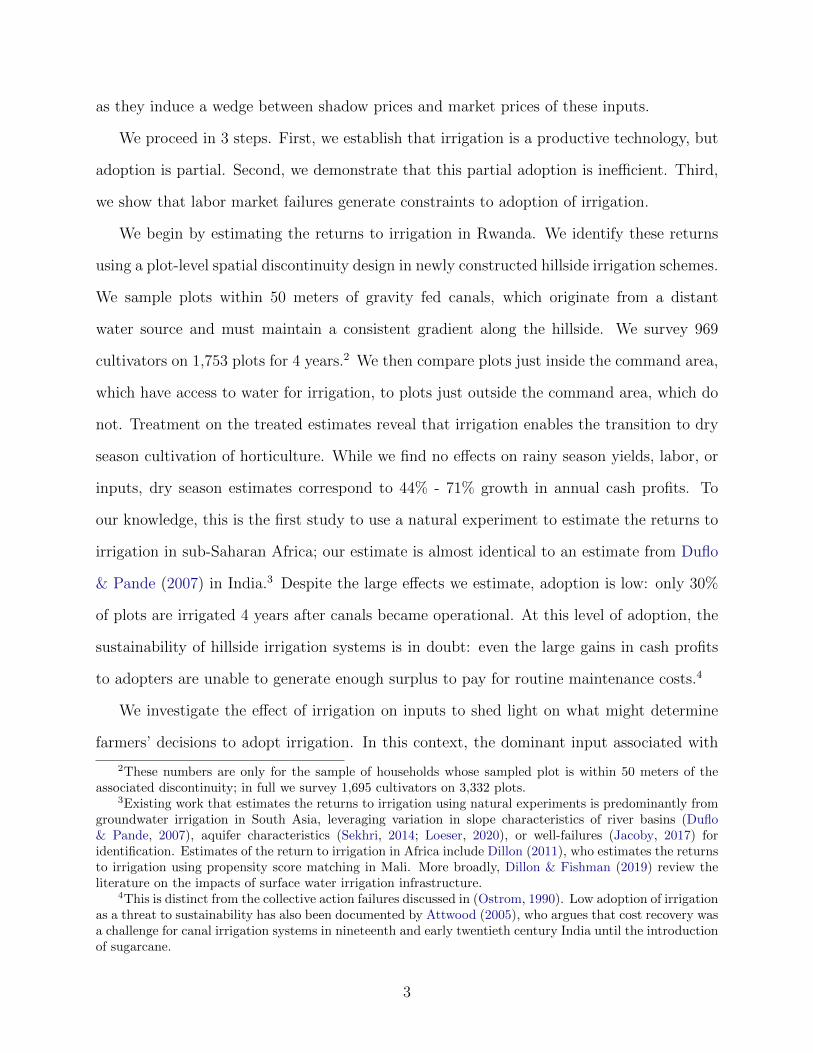
use, and on production. First, we present graphical evidence of the regression discontinuity

in Figure 5; for parsimony, we do so only for the dry seasons (2016 Dry, 2017 Dry, and 2018

Dry).23 In each of the regression discontinuity figures, distance to the canal in meters is

represented on the horizontal axis, with a positive sign indicating that the plot is on the

command area side of the boundary. Second, we present regression evidence in Tables 4, 5,

and 6. In the discussion below, we focus on results from the tables, but we note that these

results are consistent with visual intuition from Figure 5.

First, in line with results from Section 3.2.1, command area plots are 16pp - 20pp more

likely to be irrigated during the dry season than plots outside the command area, and almost

all of this increase is explained by the transition to cultivation of high value horticulture

during this dry season. In contrast, adoption of irrigation during the rainy season is much

lower, with increases of just 4pp - 6pp. This transition to dry season horticulture substitutes

for cultivation of perennial bananas, a less productive but less input intensive commercial

crop; we estimate a decrease of 13pp - 17pp in the command area, and as a consequence we

observe no impacts on overall cultivation in the dry season.24

23Rainy season differences are always smaller and generally not visually noteworthy; we focus most of ourdiscussion on the dry season results.

24As bananas are perennials, plots cultivated with bananas typically have harvests in each season. Incontrast, the rotations of staples and horticulture (or simply horticulture) that replace bananas may only

20

Second, we find large increases in dry season input use, which are dominated by increases

in household labor. These results are consistent with the transition from perennial bananas,

which require little inputs and labor, into horticulture, which is highly input and labor in-

tensive. To interpret these results, we conduct a treatment on the treated analysis under

the assumption that the command area increases input use only through its effect on irri-

gation. Doing so, we find that adoption of irrigation increases household labor use, input

expenditures, and hired labor expenditures by 340 - 450 person-days/ha, 25,000 - 39,000

RwF/ha, and 19,000 - 28,000 RwF/ha, respectively; these numbers are similar to differences

in input intensity of dry season horticulture and bananas reported in Table 1. The impacts

on household labor are particularly large – valued at a typical wage of 800 RwF/person-day,

this labor would be priced at 280,000 - 360,000 RwF/ha, an order of magnitude larger than

the effects on input expenditures or hired labor expenditures. Additionally, as reference,

applying this labor to 0.3 ha (median household landholdings) of command area land would

require roughly 4 person-months of labor during the 3 month dry season. In contrast to

these dry season results, we find no effects on input use during the rainy seasons.

Third, consistent with our estimates of impacts on input use, we find large increases in

dry season agricultural production. Treatment on the treated analysis suggests adoption

of irrigation increases yields by 300,000 - 450,000 RwF/ha, 49 - 72% of annual agricultural

production. As horticulture is primarily commercial: each 1 RwF/ha increase in yields is

associated with a 0.76 - 0.89 RwF/ha increase in sales. Once again, these results on outputs

are consistent with differences between bananas and horticulture production reported in

Table 1. Additionally, these impacts on yields are much larger than our estimates of impacts

on input and hired labor expenditures; our results suggest irrigation increases yields net

of expenditures by 250,000 - 390,000 RwF/ha, a 44 - 71% increase in annual yields net of

expenditures. However, we should not interpret this as impacts on profits, as it implicitly

places no value on the large increases in household labor. If we instead value household

involve two plantings and harvests, and we therefore see a modest decrease in cultivation during the rainyseasons of 5pp - 9pp on a baseline of 84%.

21

labor at 800 RwF/person-day, the median wage we observe, these impacts vanish completely.

Therefore, the profitability of the transition to dry season horticulture enabled by irrigation

depends crucially on the shadow wage at which household labor is valued.25

Taken together, these results suggest that irrigation leads to a large change in production

practices for a minority of farmers. Those farmers cultivate horticulture in the dry season

and a mix of horticulture, staples, and fallowing in the rainy seasons, they have substan-

tially higher earnings in the dry season but similar earnings in the other seasons, and they

invest more in inputs and much more in household labor in the dry seasons. Our estimates

suggest that irrigation has the potential to be transformative in Africa, in light of the 44

- 71% increases in yields net of expenditures that we document from just three months of

cultivation. At the same time, these results also suggest that the shadow wage, and therefore

labor market frictions, are likely to be important for the decision to cultivate horticulture.26

Building on this result, we next adapt the classical agricultural household model (Singh et al.,

1986; Benjamin, 1992) to develop formal tests for the role of market failures in adoption of

irrigation.

3.2.3 Discussion of spillovers

There are three categories of spillovers we anticipate in our context – across household

spillovers, within plot (across season) spillovers, and within household (across plot) spillovers.

The across household spillovers we anticipate are general equilibrium effects. First, as

access to irrigation increases demand for labor, we expect this to put upward pressure on

wages. Second, as access to irrigation increases sales of horticulture, we expect the prices

25In Appendix B, we estimate impacts of access to irrigation on household welfare. Although theseestimates are imprecise, all point estimates are positive and some are statistically significant. These resultsare consistent with positive impacts of access to irrigation on profits, although smaller impacts than impliedby estimates that do not value household labor.

26Testing the role of the shadow wage, by estimating the impacts of access to irrigation on profits underdifferent assumed shadow wages, has a number of limitations. First, all results above could be fully explainedby heterogeneity in the returns to adoption of irrigation (Suri, 2011). Second, person days may be a clumsymeasure for comparing hired labor and household labor, as household labor may be less intense, requirefewer hours per day, or be preferred by households to working for others.

22

of horticultural crops to decrease.27 Although our discontinuity design does not allow us

to estimate these general equilibrium effects, in Appendix C we plot wages and prices of

agricultural output by season to see if we observe any increase in wages or decrease in the

price of horticulture. While we find no evidence that wages or staple prices changed after

the hillside irrigation schemes became operational, we find some suggestive evidence that

prices of horticultural crops decreased in one of the sites.28

To interpret the impact of these potential price effects, first note that, abstracting from

within household spillovers, our estimates are the partial equilibrium effect of access to

irrigation conditional on observed wages and prices. Second, note that essentially all dry

season horticultural production in these sites is on irrigated plots. If horticulture prices

decline in these sites in response to irrigation, we therefore interpret that effects of irrigation

access on revenues and profits are smaller than they would be with frictionless trade.

The within plot (across season) spillovers we anticipate are driven by the shift out of

perennial bananas, which causes a change in patterns of cultivation during the rainy season,

while adoption of irrigation is primarily during the dry season. We estimate these spillovers

and discuss further in Section 3.2.2; we do not find strong evidence of impacts on rainy

season labor, inputs, yields, or profits.

The within household (across plot) spillovers we anticipate are driven by the increase

in demand for labor and inputs we observe on the sample plot, which may lead households

to substitute labor and inputs away from their other plots. If households face constraints,

this spillover may be first order in our context and would generate inefficiency in technology

adoption. To address this, in Section 4 we model a household’s agricultural production

27We do not anticipate general equilibrium effects in other markets would meaningfully affect our results.First, agricultural inputs are significantly more tradable than horticultural output, and we therefore donot anticipate effects on agricultural input prices. Second, although we do also find an increase in landtransactions caused by access to irrigation in Appendix G, only a small share of plots that receive access toirrigation are transacted. We therefore anticipate any general equilibrium effects through land markets tobe small.

28In section 5 we will provide evidence that farmers are optimizing labor inputs with respect to shadowwages rather than market wages. This may explain why market wages do not respond to the increased labordemand from irrigation.

23

decisions and how they can generate substitution across plots, and in Section 5 we estimate

these spillovers and quantify their implications for our estimates and for efficiency.

4 Testing for binding constraint

4.1 Model

Farmers have 2 plots, indexed by k: k = 1 indicates the sample plot, while k = 2 indicates

the most important plot. On each plot k, they have access to a simple production technology

σAkFk(Mk, Lk) where Ak is plot productivity, Mk is the inputs applied to plot k and Lk is the

household labor applied to plot k. The common production shock σ is a random variable such

that σ ∼ Ψ(σ), E[σ] = 1.29 While this specification assumes a single production function

on each plot, we can think of Fk(Mk, Lk) as the envelope of production functions from

cultivating different fractions of bananas and horticulture on the dry season; thus we will

think of cultivating bananas as optimizing at a low input intensity. Utilizing subscripts to

indicate partial derivatives and subsuming arguments we assume FkM > 0, FkL > 0, FkML >

0, FkMM < 0, FkLL < 0.30 Farmers have a budget of M which, if not utilized for inputs, can

be invested in a risk-free asset which appreciates at rate r. In this context, farmers maximize

expected utility over consumption c and leisure l, considering their budget constraint and a

labor constraint L which is allocated to labor on each plot, leisure, and up to LO units of off

farm labor LO.31 Finally, we model irrigation access as an increase in A1. As we consider

29While we refer to σ as a production shock, this incorporates general uncertainty in the value of produc-tion which includes joint price and production risk.

30Among these, FkML > 0 is the most controversial. Existing evidence on FkML in developing countryagriculture is mixed (see Heisey & Norton (2007) for discussion). In our context, we expect FkML > 0 pri-marily because Fk(·, ·) encompasses the transition from bananas to horticulture, which should be associatedwith increased labor and input demands according to Stylized Fact 2.

31We follow Benjamin (1992) in modeling incomplete labor markets as driven by an off farm labor con-straint. As in Benjamin (1992), we do so to match the observation that rural wages appear to be higher thanthe productivity of on-farm labor. However, for the predictions that follow it is sufficient that the householdfarm face an upward sloping residual labor supply. This holds if households face a downward sloping labordemand curve (implied by Benjamin (1992); alternatively, Breza et al. (2018) demonstrate the existenceof norms driven wage floors), or if households incur convex costs from working off farm (due to distastefrom working for others). Work in progress (Agness et al., 2019) attempts to separate these explanations.

24

the role of each different constraint, we develop the necessary assumptions to produce the

results from Section 3: that this increase in A1 generates an increase in demand for inputs

and labor on plot A1.

Farmers maximize expected utility

maxM1,M2,L1,L2,l,LO

E[u(c, l)]

subject to the constraints enumerated above

σA1F (M1, L1) + σA2F (M2, L2) + wLO + r(M −M1 −M2) = c

M1 +M2 ≤M

L1 + L2 + l + LO = L

LO ≤ LO

In this framework, there are three crucial constraints farmers may face that cause deviations

from expected profit maximization: access to insurance may be limited, reducing input use

to avoid basis risk; credit or access constraints may limit input use; and farmers’ off farm

labor allocations may be constrained from above, resulting in overutilization of labor on the

household farm. In analyzing model predictions we discuss the cases in which each of these

constraints do or do not bind.32

After substituting in the constraints which bind with equality, we derive the following

Alternatively, the market failure may only apply to a particular task, such as managerial labor.32These constraints correspond with those most commonly cited by farmers in focus groups as driving crop

choice. In particular, farmers frequently cite imbaraga, or strength, of the household head (corresponding tolabor market constraints), igishoro, or access to capital (corresponding to credit or input market constraints),and isoko, or access to markets (corresponding to price risk, or insurance market constraints).

25

first order conditions33

(Mk)(

1 + cov(σ,uc)E[uc]

)AkFkM = (1 + λM)r (4)

(Lk)(

1 + cov(σ,uc)E[uc]

)AkFkL = (1− λL)w (5)

(`) E[u`]E[uc]

= (1− λL)w (6)

Intuitively, the first order conditions for inputs and labor include three parts. First, each

contains the marginal product of the factor, AkFkM and AkFkL respectively, on the left hand

side, and the market price of the factor, r and w respectively, on the right hand side. The

second piece, 1 + cov(σ,uc)E[uc]

, is the ratio of the marginal utility from agricultural production to

the marginal utility from certain consumption. This ratio scales down the marginal product

of the factor. It is less than 1 because agricultural production is uncertain, and higher

in periods in which marginal utility is lower, so cov(σ, uc) < 0. With perfect insurance,

cov(σ, uc) = 0, and this piece disappears. Without it, however, farmers will underinvest in

both inputs and labor relative to the perfect insurance optimum.34 Third, there are the

Lagrange multipliers associated with the input constraint λM and with the labor constraint

λL, which scale the associated factor prices up and down, respectively.

When these constraints do not bind, and with perfect insurance, we have the familiar

result that marginal products equal marginal prices. However, if any of these constraints

bind, then separation fails: farmer characteristics which are related to λL, λM , or cov(σ, uc)

will be correlated with inefficient input allocation on all plots (inefficiently low in the case

of inputs and inefficiently high in the case of labor).

33The derivation is in Appendix D.34This result does not generically hold in models of agricultural households, as when consumption is

separately modeled, households that are net buyers of an agricultural good may overinvest in inputs andlabor relative to the perfect insurance optimum (Barrett, 1996). This is unlikely to be first order in ourcontext, as we sampled cultivators and our results are driven by production of commercial crops.

26

4.2 A test for separation failures

In this context, we consider a new test of separation: the effect of a change in access to

irrigation on the sample plot on production decisions on the most important plot. Much of

the literature that tests for separation, building on Benjamin (1992), has focused on tests

built around the assumption that household characteristics should not affect the household’s

optimal production decisions under perfect markets. We instead leverage the assumption

that access to irrigation on the sample plot (the “sample plot shock”) should not affect the

optimal production decisions on the household’s most important plot.

Following our model, we show how these market failures in insurance, labor, or input

markets generate a separation failure between production decisions on the sample plot and

production decisions on the most important plot. First, we derive the classic separation

result from Singh et al. (1986) in our framework when there are no market imperfections.

Proposition 1. If no constraint binds, separation holds and input and labor use on the most

important plot does not respond to the sample plot shock.

Showing this result is straightforward: with perfect markets for inputs, labor, and insur-

ance, cov(σ,uc)E[uc]

= 0, λL = 0, and λM = 0, respectively. The first order conditions then simplify

to

(Mk) AkFkM = r

(Lk) AkFkL = w

(`) E[u`]E[uc]

= w

The household’s labor and input allocations on plot 2 depend only on plot 2 productivity

A2, the price of inputs r, and the wage w, and not on access to irrigation on plot 1 (A1).

In contrast to the case with perfect markets, in the presence of market failures, the sample

plot shock can affect the households allocations on its most important plot. Roughly speak-

ing, the sample plot shock increases the household’s agricultural production, and increases

27

its labor and input demands on the sample plot. When markets fail, this reduces the value

the household places on agricultural production, and increases its opportunity costs of labor

and inputs, and the household reduces its labor and input allocations on its most important

plot. The following propositions require additional assumptions on the shape of the utility

function or on the distribution of σ; we highlight those in the text below each proposition.

Proposition 2. If input, labor, or insurance constraints bind, then input and labor use are

reduced on the most important plot in response to the sample plot shock.35

The logic case-by-case is as follows. First, if input constraints bind, then the increase in

inputs on the sample plot caused by access to irrigation must be associated with a reduction

in inputs on the most important plot. As inputs and labor are complements, this causes labor

allocations on the most important plot to fall as well. Second, if labor constraints bind, then

the increase in labor on the sample plot caused by access to irrigation must be associated

with a reduction in the sum of leisure and labor on the most important plot. Under standard

restrictions on the household’s on farm labor supply, this must be associated with a reduction

in labor on the most important plot.36 As inputs and labor are complements, this causes

input allocations on the most important plot to fall as well. Third, absent insurance, then

the increase in agricultural production caused by access to irrigation reduces the marginal

utility from agricultural production relative to the marginal utility from consumption.37 In

turn, this causes labor and input allocations to the most important plot to fall.

An implicit assumption we make that generates this result is the absence of function-

ing land markets. With perfectly functioning land markets, shocks to the household’s land

endowment, such as the sample plot shock, should not affect productive decisions on the

household’s most important plot. Instead, both the sample plot and most important plot

35See proof in Appendix D.36Specifically, we assume that leisure demand is increasing in consumption; this assumption is not neces-

sary but is sufficient.37This does not generically hold; however, restrictions on the distribution of σ are sufficient to imply that

marginal utility from agricultural production relative to the marginal utility from consumption is falling inagricultural production. Details are in Appendix D.

28

would flow to the household with the highest willingness-to-pay for them. In practice, land

transactions do occur; as discussed in Section 2.2.2, our survey tracks plots across transac-

tions in land markets, so we are able to directly test the prediction that the sample plot

shock does not affect the productive decisions on the most important plot itself.

Proposition 2 produces a test of separation. Rejecting separation with this test implies

that the levels of irrigation adoption are inefficient and that land market failures contribute

to this inefficiency. At the same time, this test does not allow us to test for which other con-

straints interact with land market frictions to generate separation failures. This is because

the presence of any set of constraints that generate separation failures yields the same predic-

tion: the sample plot shock should cause input and labor allocations on the most important

plot to fall. In particular, the intuition that observing changes in input allocations, labor

allocations, or cropping decisions on the most important plot might suggest the presence

of input constraints, labor constraints, or insurance constraints, respectively, fails, because

inputs, labor, and horticulture are all complements in the production function.

4.3 Separating constraints

To shed light on which other constraints generate separation failures, we leverage the fact

that our model offers predictions about how households with different characteristics should

differentially respond to the sample plot shock. Roughly speaking, depending on which

constraint binds, changes in different household characteristics may slacken or tighten the

binding constraint. We focus on two important household characteristics in our model: we

use household size to shift L, the household’s total available labor, and wealth to shift M , the

household’s exogenous income available for input expenditures. We present these predictions

below.

Proposition 3. If input constraints or insurance constraints bind, then the input and labor

allocations on the most important plot of larger households (wealthier households) should be

29

less (less) responsive to the sample plot shock.38

Under insurance constraints, both wealth and household size enter the model symmetri-

cally by increasing consumption; therefore, in all cases, wealthier and larger households will

respond similarly to the sample plot shock. If we additionally assume that risk aversion is

decreasing sufficiently quickly in consumption, then the allocations of wealthier and larger

households will be closer to those maximizing expected profits, and therefore allocations on

the most important plot will be less responsive to the sample plot shock.

Under input constraints, wealthier households are less likely to see the constraint bind.

As the allocations on the most important plot of unconstrained households do not respond

to the sample plot shock, wealthier households should be less responsive. Now, note that

in this model, farmers cannot use labor income to purchase additional inputs. In a more

general model with borrowing, they may be able to; in that case, both wealthier households

and larger households are less likely to see the constraint bind, and therefore will both be

less responsive to the sample plot shock on their most important plots.39

Proposition 4. If labor constraints bind, then the relative responsiveness of input and labor

allocations on the most important plot of larger households (wealthier households) to the sam-

ple plot shock cannot be signed without further assumptions. If larger households and poorer

households have more elastic on farm labor supply schedules, and if on farm labor supply

exhibits sufficient curvature, then the input and labor allocations on the most important plot

of larger households (wealthier households) should be less (more) responsive to the sample

plot shock.40

When labor constraints bind, the household responds to the sample plot shock by allo-

cating additional labor to the sample plot, but they may withdraw that labor from either

38See proof in Appendix D.39If all households are input constrained, then the effect of the sample plot shock on input allocations

on the most important plot depends on characteristics of the production function. Note that in this case,larger households will still exhibit a response in the same direction as wealthier households as both effectsenter only through the wealth channel.

40See proof in Appendix D.

30

the most important plot or from leisure. Whether wealthier or larger households withdraw

relatively more labor from the most important plot depends on the higher order derivatives

of the utility and production functions; in general, these differential responses can not be

signed.41 Additionally, one key difference from the insurance case and input case is that

household size and wealth no longer enter the model symmetrically. In one sense, household

size and wealth instead enter the model as opposing forces: wealthier households allocate

less labor to their plots, as they value leisure relatively more than consumption, while larger

households allocate more labor to their plots.

We focus on one particular case that builds on this intuition, presented in Figure 6.

When on farm labor supply exhibits sufficient curvature, then changes in responsiveness to

the sample plot shock of allocations on the most important plot are dominated by changes

in the elasticity of on farm labor supply. Suppose this to be the case, and further suppose

that the elasticity of on farm labor supply is decreasing in the shadow wage. As we can

think of household size as shifting out on farm labor supply (by increasing L), and wealth

as shifting in on farm labor supply (by increasing the marginal utility of leisure relative to

the marginal utility of consumption), then larger households are located on a more elastic

portion of their on farm labor supply schedule, while wealthier households are located on a

less elastic portion of their on farm labor supply schedule.42 As a result, larger households

will be less responsive to the sample plot shock, as they will primarily draw labor on the

sample plot from leisure, while wealthier households will be more responsive to the sample

plot shock, as they will primarily draw labor on the sample plot from the most important

plot.

These predictions of the model, summarized in Table 7, generate a test that allows us to

reject the absence of labor constraints. In particular, note that while insurance constraints

or input constraints can rationalize the allocations of wealthier households to their most

41Of course, the potential for ambiguous responses is heightened further if other forms of labor constraints,for example on hiring labor, are also considered.

42This relationship between household size, wealth, and on farm labor supply elasticity has been positedas far back as Lewis (1954), and is discussed in depth in Sen (1966).

31

important plot as less responsive to the sample plot shock, only the presence of labor con-

straints can rationalize them as more responsive to the sample plot shock. Additionally,

note that the model would struggle to rationalize larger households as more responsive to

the sample plot shock, although it is possible to do so in the presence of labor constraints. In

sum, we would interpret observing larger households as (weakly) less responsive and richer

households as less responsive to the sample plot shock as most consistent with the presence

of either input or insurance constraints, observing larger households as less responsive and

richer households as more responsive as evidence for the presence of labor constraints, and

observing larger households as more responsive as inconsistent with our model.

5 Separation failures and adoption of irrigation

5.1 Empirical strategy

Our first specification to test for separation failures mirrors Equation (1), which we use to

estimate the impacts of irrigation. We still make use of the discontinuity across the command

area boundary, but outcomes are now on the household’s most important plot (plot 2) instead

of the sample plot (plot 1).

y2ist = β0 + β1CA1is + αst + ε2ist (7)

We report β1, the effect of the sample plot shock on outcomes on the most important plot.

In other specifications, we also consider heterogeneity with respect to the location of the

most important plot, and include CA1is ∗ CA2is to test for this. In these specifications, we

also report this difference in differences coefficient. For both this coefficient and β1, in line

with the model predictions in Table 7, we interpret negative coefficients on labor, inputs,

irrigation use, and horticulture, as evidence of separation failures.

As in Section 3, we include specifications with progressively more controls. Specifically,

32

we also estimate

y2ist = β0 +β1CA1is+β2Dist1is+β3CA1is∗Dist1is+β4CA2is+γ1X1is+γ2X2is+αst+ε2ist (8)

y2ist − y2ist = β1(CA1is − CA1is) + (V1is − V 1is)′γ1 + (V2is − V 2is)

′γ2 + (ε2ist − ε2ist) (9)

Equation (8) includes controls CA2is, an indicator for whether the most important plot is

in the command area, and X1is and X2is, the log area of the sample plot and the most

important plot, respectively. Equation (9) uses spatial fixed effects, as described in Section

3.1.43

Our benchmark specification to test for which constraints drive the separation failures is

similar, but also includes the interaction of households characteristics with the sample plot

shock. For parsimony, we only present the specification of this interaction for a specification

similar to Equation (8); all tables present results with interactions included in Equation (7)

and Equation (9) similarly.

y2ist = β0 + β1CA1is +W ′iβ2 + CA1is ∗W ′

iβ3 + β4Dist1is + β5CA1is ∗Dist1is

+β6CA2is + γ1X1is + γ2X2is + αst + ε2ist (10)

where Wi is a vector of household characteristics, which includes household size and an asset

index in our primary specifications.44 We focus on β3: the heterogeneity, with respect to

household characteristics, of the impacts of the sample plot shock on outcomes on the most

important plot. The signs on β3 give our main test of which market failures cause separation

43Note that all differencing in this specification is done using the location of sample plots; in other words,most important plots whose associated sample plots are near each other are compared, as opposed to mostimportant plots which are near each other.

44An implicit assumption we make when interpreting the results from this specification is that householdsize and asset index are not correlated with other household or plot characteristics that might affect patternsof substitution. To test this, in results available upon request, we have included other household and plotcharacteristics in the interaction that might affect these patterns – number of plots and number of commandarea plots (if households with more land are more price risk averse), and plot area (as a proxy for quality, ifsmaller plots are typically higher quality). None of these added controls affect the significance of our results.

33

failures; Table 7 presents which signs map to which market failures.

5.1.1 Balance

We now use specifications (7), (8), and (9) to examine whether the most important plots in

our sample are comparable for households whose sample plot is just inside or just outside

the command area. As in Section 3.1.1, for each of these specifications, we show balance

both with key controls omitted (Columns 3, 5, and 6), and our preferred specifications which

we use in our analysis with key controls included (Columns 4, 7, and 8). Balance tests for

most important plots are reported in Table 8. First, note that specifications that do not

restrict to the discontinuity sample perform particularly poorly here. Most notably, most

important plots are more likely to be located in the command area when sample plots are

also located in the command area, as households’ plots tend to be located near each other.

In contrast, our preferred specifications (Columns 4, 7, and 8, Table 8) which restrict to the

discontinuity sample correct for this imbalance. Otherwise, we have a p-value of less than 0.1

for one variable in Column 4 (an indicator for owning the plot); for all three specifications,

the omnibus test fails to reject the null of balance.

As an additional check, in Appendix F, we estimate for 2014 Dry specifications (7), (8),

and (9), and specifications with heterogeneity following Equation (10). As the command

area, as of the baseline, had not yet caused a large increase in demand for labor or inputs,

or caused large increases in agricultural production, we would not anticipate any effects on

MIPs. In line with this prediction, we fail to find any consistent significant effects on MIPs,

either in our main specifications or for heterogeneity.

34

5.2 Results

5.2.1 A test for separation failures

We now present results on separation failures, demonstrating that the sample plot shock

causes farmers to substitute away from their most important plot.45 First, we present graph-

ical evidence of this substitution in Figure 7. As in earlier figures, distance of the sample plot

to the canal in meters is represented on the horizontal axis, with a positive sign indicating

that the plot is on the command area side of the boundary. However, we now plot outcomes

on both the sample plot and the most important plot. In this figure, substitution will man-

ifest as decreases in input and labor use on the most important plot when the sample plot

is in the command area, while input and labor use increase on the sample plot. Second, we

present regression evidence in Tables 9, 10, and 11. In the discussion below, we focus on

results from the tables, but we note that these results are consistent with visual intuition

from Figure 7.

First, consistent with the presence of separation failures, in Columns 3 through 5 we find

households substitute labor and inputs away from their most important plot. Households

decrease allocations of household labor (11 - 33 person-days/ha) and inputs (2,100 - 6,700

RwF/ha) on their most important plot in response to the sample plot shock. Additionally,

they substitute away from labor and input intensive technologies, consistent with our in-

terpretation of the production function as the envelope of production functions across crop

choices. Households decrease use of irrigation (1.9 - 4.4pp) and cultivation of horticulture

(1.6 - 3.8pp), while increasing cultivation of bananas (6.5 - 9.2pp).46

45We present results only for the dry seasons (2016 Dry, 2017 Dry, and 2018 Dry), because these are theprimary seasons for irrigation use, during which we anticipate substitution effects. Additionally, we presentresults only on cultivation decisions and input use, because we expect these substitution effects to be smallerthan the direct effects and therefore we do not anticipate being able to detect effects on output. Theseadditional results are available upon request.

46While these results are not consistently statistically significant, the specifications used lose power byincluding most important plots outside the command area, which are almost never irrigated and have smallallocations of labor and inputs during the dry season. As discussed in the next paragraph, specifications whichinclude the interaction of the sample plot command area indicator with a most important plot commandarea indicator are more precise for irrigation use, horticulture cultivation, and labor and input use.

35

Next, we expect the results above to be driven primarily by most important plots located

in the command area for most outcomes. This is because there is limited irrigation, and

therefore input use or horticulture during the dry season, on plots that cannot be irrigated.

Consistent with this, in Columns 6 through 8, we find our results on irrigation, horticulture,

and inputs are all driven by plots located in the command area. When the most important

plot is located in the command area, the 16 - 20pp increase in irrigation use on sample plots in

the command area coincides with a 8 - 10pp decrease in irrigation use on the most important

plot; these relative magnitudes suggest that separation failures cause few households to be

able to use irrigation on more than one plot in the command area.

As discussed in Section 3, the direct effects of the command area appear driven by

enabling the transition to dry season horticultural cultivation and substitution away from

lower value banana cultivation. However, the model in Section 4 is agnostic about whether

decreases in labor and input allocations on the most important plot are driven by extensive

margin responses (i.e., decreases in horticulture) or intensive margin responses (i.e., decreases

in labor and input allocations conditional on crop choice). To test this, in Tables A1 and

A2, we present results of the sample plot shock on labor and input use on sample plots

and most important plots, controlling for cultivation and crop choice.47 Table A1 confirms

that the effects we document in Section 3 are driven by the shift to dry season horticulture,

as effects on sample plots all but disappear controlling for crop choice. However, Table

A2 suggests that much of the effect of the sample plot shock on labor and input use on

most important plots is driven by intensive margin responses, as coefficients on household

labor and inputs fall by only 18% - 36%. Combined with our results on irrigation use and

horticulture, this suggests that households respond to the sample plot shock on both the

intensive and extensive margins on their most important plot.

47As crop fixed effects are a “bad control” (Angrist & Pischke, 2008), which introduces selection bias, weinterpret these results as suggestive. However, we anticipate that selection conditional on crop choice shouldbias us towards finding no intensive margin effect on most important plots, as the particularly constrainedhouseholds switching out of horticulture in response to the sample plot shock are likely to be the householdswho used less labor and inputs.

36

These results on separation failures imply the existence of a within-household negative

spillover, as they show that having one additional plot in the command area causes a house-

hold to substitute away from their other plots, reducing their use of irrigation, labor, and

inputs on those plots. In principle, this means that our estimates of the impacts of irriga-

tion are the impacts of irrigating one of a farmers’ plots, gross of any input reallocations

made by the farmers across plots in response to that irrigation. We would be particularly

concerned about the bias generated by these reallocations if inputs were being shifted out of

production on non-irrigated plots: in that case, our estimated impacts of access to irrigation

would include reduced farming intensity on non-irrigated plots. However, the substitution

of inputs we estimate from most important plots outside the command area is generally not

significantly different from zero, and the largest point estimate implies it is 37% as large as

substitution away from command area plots.48 We therefore conclude that the dominant

within-household spillover is a reduced intensity of cultivation on irrigated plots. This sug-

gests any bias in our estimates caused by spillovers onto plots outside the command area

is likely to be small, and that spillovers onto plots inside the command area decreases our

estimates in Section 3.

5.2.2 Impacts of separation failures on adoption of irrigation

We now quantify the impact of separation failures on adoption of irrigation. We ask what

would happen to adoption of irrigation if all households with two or more plots in the

command area only had one plot in the command area. This counterfactual follows naturally

from our estimates of the effect of the sample plot shock on adoption of irrigation on the

most important plot, which we can interpret as the effect of a household’s second plot (the

sample plot) being moved to the command area on adoption of irrigation on its first plot in

the command area (the most important plot).

48We calculate this using β1/(β1 +β3,CA) from Equation 10, the impact of the sample plot shock on inputallocations on most important plots outside the command area divided by the impact on most importantplots inside the command area. Estimates come from Columns 6 - 8 in Table 11.

37

Specifically, we calculate

(# of HH with 2 CA plots) ∗ 2 ∗ (β1 + β3,CA)

(# of HH with 2 CA plots) ∗ 2 + (# of HH with 1 CA plot)

First, (β1 +β3,CA) (from Equation 10) is the total effect of the sample plot shock on adoption

of irrigation on most important plots in the command area. Second, in the denominator, we

count the total number of command area plots among households’ sample plots and most

important plots.49 Third, in the numerator, we apply the estimated substitution caused by

the sample plot shock to both the sample plot and the most important plot, as households

are also substituting away from their sample plot when the most important plot is in the

command area.

We find adoption of irrigation would be 21% - 24% higher under this counterfactual.

This counterfactual relates to land market frictions – absent these frictions, we would expect

that the increased adoption of irrigation caused by this reallocation would be achieved by

land markets. Intuitively, under perfect land markets, characteristics of the household that

manages a particular command area plot at baseline, including the number of other command

area plots that household managed at baseline, should not affect equilibrium adoption of

irrigation on that plot. Relatedly, as shown in the model, this would also be true if all

markets (except potentially land markets) were frictionless.

5.2.3 Separating constraints

We now provide evidence on the source of the separation failure by estimating heterogeneous

impacts, with respect to household size and wealth, of the sample plot shock on outcomes on

the most important plot. Recall that for this analysis, the key predictions of the model were

1) if only insurance or input constraints bind, wealthier households and larger households

should be less responsive, and 2) if only labor constraints bind, differential responsiveness of

49We implicitly ignores households’ other plots; we do so because our research design has little to sayabout the impacts of additional command area plots, or on households’ behavior on these plots, so weinterpret this exercise as estimating a lower bound on the impact of reallocation on adoption of irrigation.

38

wealthier and larger households is ambiguous, but under reasonable assumptions wealthier

households should be more responsive and larger households should be less responsive. Note

that this test does not allow us to reject a null that a particular constraint exists; any pattern

of differential responses is consistent with all constraints binding. However, if we observe

that wealthier households are more responsive, we can reject the null of no labor constraints.

Additionally, we would interpret observing wealthier households to be more responsive and

larger households to be less responsive as the strongest evidence of the presence of labor

constraints from this test.

We present the results of this test in Tables 12 and 13. First, larger households are less

responsive to the sample plot shock across every outcome. A household with 2 additional

members, approximately one standard deviation of household size, is less responsive to the

sample plot shock on its most important plot by 50% - 94% for irrigation use, 74% - 103%

for horticulture, 63% - 75% for household labor, and 20% - 21% for inputs, with all but

the input coefficient statistically significant and robust across specifications.50 In contrast,

wealthier households are more responsive to the sample shock across these same outcomes.

A household with a one standard deviation higher asset index is more responsive to the

sample plot shock on its most important plot by 41% - 97% for irrigation use, 39% - 81%

for horticulture, 39% - 72% for household labor, and 42% - 58% for input use; however,

these results are less precise. In effect, these results suggest that our estimates of separation

failures are driven by the behavior of small, rich households, while large, poor households

do not change their allocations on their most important plot in response to the sample plot

shock. As discussed in Section 4.3, these results are very difficult to reconcile with a model

that does not feature labor market failures.

In sum, these results provide strong evidence for the existence of labor market failures

that generate separation failures, which in turn cause inefficient adoption of irrigation.

50These percentages, and the remainder of percentages in this paragraph, are expressed relative to the esti-mated impact of the sample plot shock on the most important plot, and are calculated only for Specifications(8) and (9).

39

6 Experimental evidence

Our results leveraging the discontinuity suggest that land and labor market frictions combine

to constrain the adoption of hillside irrigation in Rwanda. We design and run three experi-

ments to test for the presence of other constraints to adoption of irrigation – specifically, we

focus on operations and maintenance of irrigation schemes, and financial and informational

constraints. These experimental results corroborate that labor market failures are a primary

constraint to adoption of irrigation in this context. Additional details on the motivation,

treatment assignment protocols, and logistics of implementation of each of these experiments

are presented in Appendix E.

First, we test whether failures of operations and maintenance impose a constraint that

limits farmers’ adoption of irrigation. The government implementing agency designed a

centralized O&M system to establish and enforce water usage schedules to ensure farmers’

access to water. If farmers faced limited access to water due to problems in the operations

and maintenance system, this could constrain adoption of irrigation. We sought to alleviate

this potential constraint by randomizing empowerment of local monitors to assist system

operators and report maintenance needs. We find no evidence this experiment changed

cultivation practices. This result is likely because very few farmers report any challenges

related to operations and maintenance over the four years of survey data collection. Second,

the government planned to charge farmers in the command area land taxes, which were

unconditional on cultivation decisions, to fund operations and maintenance in the schemes.

To test whether these fees would limit farmers adoption of irrigation, we randomized subsidies

of farmers’ fees. We find no evidence this experiment changed cultivation practices. This

result is likely because compliance with the fees was extremely low (4%), so collected fees were

too low to plausibly constrain farmers. We discuss these experiments further in Appendix

E.2, and conclude here that these issues were not relevant in this context.

Third, we test whether financial and informational constraints limit adoption of irriga-

tion. To do so, we assigned horticultural minikits to randomly selected farmers from water

40

user group member lists. Each minikit included horticultural seeds, chemical fertilizer, and

insecticide, in sufficient quantities to cultivate 0.02 ha. In principle, these minikits should

resolve constraints related to input access, including credit constraints. In addition, they

should reduce basis risk which may resolve insurance constraints. Lastly, they should facili-

tate experimentation and increase adoption if information is a constraint. In other contexts,

minikits of similar size relative to median landholdings have been shown to increase adop-

tion of new crop varieties or varieties with low levels of adoption (Emerick et al., 2016; Jones

et al., 2018). To test for spillovers, water user groups were randomly assigned to 20%, 60%,

or 100% minikit saturation, with rerandomization for balance on Zone and O&M treatment

status. Minikits were offered to assigned individuals prior to 2017 Rainy 1 and 2017 Dry.51

6.1 Empirical strategy and results

We estimate the impact of minikits using the specification

y1ist = β0 + β1Assigned minikiti + β2Minikit saturationi +X ′1isγ + ε1ist (11)

Assigned minikiti is a dummy for whether household i was randomly assigned to receive a

minikit, Minikit saturationi is the probability of receiving a minikit for households in the

water user group of household i’s sample plot, and X1is includes the stratification variables

(Zone fixed effects and O&M treatment status), as well as indicator variables reflecting the

probability that a household would receive a minikit52 and in some specifications 2016 Dry

51Each of these three interventions exist only in the command area. As such, the effects of irrigationestimated throughout this paper are averages across the experimental treatments. Overall, this concernis mitigated by the fact that all three experimental treatments had very limited impacts on cultivationpractices. In addition, the first two of these treatments (fee subsidies and monitoring systems) vary char-acteristics which would be heterogeneous across different irrigation systems; we are therefore comfortablewith the interpretation that estimates above exist for the average of these treatments. Readers may be mostconcerned about interpretations of treatment effects in the presence of the minikit treatment; in addition tothe modest effects on cultivation described below, we have also conducted analysis excluding minikit winnersand conclusions are qualitatively unaffected.

52After matching names from the lists of water user group members to our baseline survey, we found that32% of households either had multiple household members on the lists of water user group members or hada single household member listed multiple times; these households are more likely to be assigned to receive

41

horticulture adoption. As minikit saturation is assigned at the water user groups level,

robust standard errors are clustered at the water user group level.

For our primary outcomes y, we focus on whether households used a minikit (in 2017

Rainy 1 or in 2017 Dry) and adoption of horticulture. Impacts on minikit use are our first

stage and impacts on adoption of horticulture are our measure of learning from the minikits.

For precision, we restrict to command area plots, and for plot level outcomes we focus on

2017 Dry and 2018 Dry; these are the plots and seasons in which we expect households to

adopt horticulture in response to being assigned a minikit.

We present the results of this analysis in Table 14. First, we find a strong first stage;

households assigned to receive a minikit are 40pp more likely to use a minikit than households

not assigned to receive a minikit. Almost all non-compliance is driven by households who

were assigned to receieve a minikit but did not pick it up – 4.8% of households not assigned to

received a minikit used one, while 43.8% of households assigned to receive a minikit used one.

Second, we find no effects of minikits on horticulture use, and we have sufficient precision to

reject estimates from other contexts of the effect of minikits on technology adoption (Emerick

et al., 2016; Jones et al., 2018). Third, consistent with this null effect on horticulture use,

we find no effects of minikit saturation, although these estimates are less precise than those

of the impacts of assignment to receive a minikit; we note that we also fail to reject that the

sum of the coefficients on assigned minikit and minikit saturation (the effect on adoption in

a fully treated compared to an untreated water user group) is zero. Fourth, we find strong

positive selection into using a minikit: farmers who grew horticulture in 2016 Dry, who are

30.6pp more likely to grow horticulture in 2017 and 2018 Dry, are 13.1pp more likely to use

a minikit in response to assignment to receieve a minikit receipt.

We interpret these results as corroborating evidence that information and financial con-

straints are not dominant constraints to adoption of irrigation. Most farmers assigned to

receive a minikit do not pick it up and use it, and the farmers who do pick it up typically

a minikit and may differ from other households

42

would have grown horticulture even if not assigned to receive a minikit. We similarly find

no evidence that saturation of minikits lead to increased adoption, as we might expect if

learning was important.53 Our experimental evidence therefore supports the conclusion that,

in this context, financial and informational frictions are not the primary explanations for the

low and inefficient irrigation use we observe.

7 Conclusions

This paper provides evidence that irrigation has the potential to be a transformative technol-

ogy in sub-Saharan Africa. Using data from very proximate plots which receive differential

access to irrigation, we document that the construction of an irrigation system leads to a

44% - 71% increase in cash profits. These profits are generated by a switch in cropping

patterns from perennial bananas towards a rotation of dry-season horticulture and rainy-

season staples, which itself is associated with an increase in input intensity. In our context,

the primary increase in input demands is for household labor, which is used intensively on

horticulture and minimally on banana cultivation.

These results suggest that irrigation may have similar potential in Africa to the transfor-

mative role it played in South Asia, where other studies have documented similar impacts of

irrigation on farmer revenues and yields. In some ways, this is surprising: other evidence on

the use of inputs in Africa and the returns to those inputs often finds lower usage and tech-

nological returns in the African context. These two facts together suggest that expanding

irrigation access in Africa may be a necessary contributor to shrinking the yield gap.

At the same time, even with access to a new, highly productive technology provided

freely by the government we observe a minority of farmers adopting this technology four

years after introduction. Given the returns identified above, we take this as evidence that

the existence of a productive technology is not itself sufficient to generate majority adoption

53That information is not a binding constraint is also consistent with the stability in levels of irrigationadoption that we observe over time, in contrast to an S-curve of adoption which would be consistent withlearning.

43

in all agricultural contexts. We further document that frictions in land and labor markets

contribute to low utilization of irrigation systems by examining farmers’ input utilization

on other plots in response to irrigation investments. This result provides novel evidence

that separation failures in agricultural household production lead to land misallocation and

inefficient adoption of a new technology in Rwanda.

These results highlight the need for more evidence on both the role of factor markets

in technology adoption, and the identification of particular institutions which contribute

to or which can smooth those market failures. In some cases, these market failures may

pose a competing constraint which coexists with other, more conventional constraints to

production: if frictions in factor markets similarly constrain adoption of new technologies in

other environments, then incomplete factor markets may generate limits to the effectiveness

of financial and information interventions in improving agricultural productivity.

44

References

Adamopoulos, T., Brandt, L., Leight, J., & Restuccia, D. (2017). Misallocation, Selection

and Productivity: A Quantitative Analysis with Panel Data from China. Working Paper

23039, National Bureau of Economic Research.

Adamopoulos, T. & Restuccia, D. (2014). The size distribution of farms and international

productivity differences. American Economic Review, 104(6), 1667–97.

Adamopoulos, T. & Restuccia, D. (2018). Geography and Agricultural Productivity: Cross-

Country Evidence from Micro Plot-Level Data. Working Paper 24532, National Bureau of

Economic Research.

Agness, D., Baseler, T., Chassang, S., Dupas, P., & Snowberg, E. (2019). Wages and the

value of time in rural labor markets. AEA RCT Registry.

Ali, D. A., Deininger, K., & Goldstein, M. (2014). Environmental and gender impacts of

land tenure regularization in africa: Pilot evidence from rwanda. Journal of Development

Economics, 110, 262–275.

Anderson, M. (2008). Multiple inference and gender differences in the effects of early inter-

vention: A reevaluation of the abecedarian, perry preschool, and early training projects.

Journal of the American Statistical Association, 103(484), 1481–1495.

Angrist, J. D. & Pischke, J.-S. (2008). Mostly harmless econometrics: An empiricist’s com-

panion. Princeton university press.

Attwood, D. W. (2005). Big is ugly? how large-scale institutions prevent famines in western

india. World Development, 33(12), 2067–2083.

Barrett, C. B. (1996). On price risk and the inverse farm size-productivity relationship.

Journal of Development Economics, 51(2), 193–215.

45

Benjamin, D. (1992). Household composition, labor markets, and labor demand: testing for

separation in agricultural household models. Econometrica: Journal of the Econometric

Society, (pp. 287–322).

Besley, T. (1995). Property rights and investment incentives: Theory and evidence from

ghana. Journal of Political Economy, 103(5), 903–937.

Besley, T. & Ghatak, M. (2010). Property rights and economic development. In Handbook

of development economics, volume 5 (pp. 4525–4595). Elsevier.

Bleakley, H. & Ferrie, J. (2014). Land openings on the georgia frontier and the coase theorem

in the short-and long-run.

Breza, E., Krishnaswamy, N., & Kaur, S. (2018). Scabs: The social suppression of labor

supply.

Conley, T. G. (1999). Gmm estimation with cross-sectional dependence. Journal of Econo-

metrics, 92(1), 1–45.

Conley, T. G. & Udry, C. R. (2010). Learning about a new technology: Pineapple in ghana.

The American Economic Review, (pp. 35–69).

De Janvry, A., Sadoulet, E., & Suri, T. (2017). Field experiments in developing country

agriculture. In Handbook of Economic Field Experiments, volume 2 (pp. 427–466). Elsevier.

Deininger, K. & Feder, G. (2009). Land registration, governance, and development: Evidence

and implications for policy. The World Bank Research Observer, 24(2), 233–266.

Dillon, A. (2011). The effect of irrigation on poverty reduction, asset accumulation, and

informal insurance: Evidence from northern mali. World Development, 39(12), 2165–2175.

Dillon, A. & Fishman, R. (2019). Dams: Effects of hydrological infrastructure on develop-

ment. Annual Review of Resource Economics, 11.

46

Dillon, B. & Barrett, C. B. (2017). Agricultural factor markets in sub-saharan africa: An

updated view with formal tests for market failure. Food policy, 67, 64–77.

Dillon, B., Brummund, P., & Mwabu, G. (2019). Asymmetric non-separation and rural labor

markets. Journal of Development Economics, 139, 78–96.

Duflo, E. & Pande, R. (2007). Dams. The Quarterly Journal of Economics, 122(2), 601–646.

Emerick, K., de Janvry, A., Sadoulet, E., & Dar, M. H. (2016). Technological innovations,

downside risk, and the modernization of agriculture. American Economic Review, 106(6),

1537–61.

Fafchamps, M. (1993). Sequential labor decisions under uncertainty: An estimable household

model of west-african farmers. Econometrica, 61, 1173–1197.

Fei, J. C. & Ranis, G. (1961). A theory of economic development. The American Economic

Review, 51(4), 533–565.

Foster, A. & Rosenzweig, M. (2017). Are there too many farms in the world? labor-market

transaction costs, machine capacities, and optimal farm size. NBER Working Paper, (No.

23909).

Goldstein, M., Houngbedji, K., Kondylis, F., O’Sullivan, M., & Selod, H. (2018). Formal-

ization without certification? experimental evidence on property rights and investment.

Journal of Development Economics, 132, 57–74.

Goldstein, M. & Udry, C. (2008). The profits of power: Land rights and agricultural invest-

ment in ghana. Journal of political Economy, 116(6), 981–1022.

Gollin, D. & Udry, C. (2019). Heterogeneity, measurement error and misallocation: Evidence

from african agriculture. NBER Working Paper 25440.

Heisey, P. W. & Norton, G. W. (2007). Fertilizers and other farm chemicals. Handbook of

agricultural economics, 3, 2741–2777.

47

Jacoby, H. G. (1993). Shadow wages and peasant family labour supply: an econometric

application to the peruvian sierra. The Review of Economic Studies, 60(4), 903–921.

Jacoby, H. G. (2017). “well-fare” economics of groundwater in south asia. The World Bank

Research Observer, 32(1), 1–20.

Jones, M., Kondylis, F., Mobarak, A. M., & Stein, D. (2018). Evaluating the integrated

agriculture productivity project in bangladesh.

Karlan, D., Osei, R., Osei-Akoto, I., & Udry, C. (2014). Agricultural decisions after relaxing

credit and risk constraints. The Quarterly Journal of Economics, 129(2), 597–652.

Kaur, S. (2014). Nominal wage rigidity in village labor markets. NBER Working Paper

20770.

Key, N., Sadoulet, E., & Janvry, A. D. (2000). Transactions costs and agricultural household

supply response. American journal of agricultural economics, 82(2), 245–259.

LaFave, D. & Thomas, D. (2016). Farms, families, and markets: New evidence on complete-

ness of markets in agricultural settings. Econometrica, 84(5), 1917–1960.

Lewis, W. A. (1954). Economic development with unlimited supplies of labour. The manch-

ester school, 22(2), 139–191.

Loeser, J. (2020). India’s groundwater revolution and agricultural productivity.

Magruder, J. (2012). High unemployment yet few small firms: The role of centralized

bargaining in south africa. American Economic Journal: Applied Economics, 4(3), 138–

66.

Magruder, J. (2013). Can minimum wages cause a big push? evidence from indonesia.

Journal of Development Economics, 100(1), 48–62.

48

Ostrom, E. (1990). Governing the commons: The evolution of institutions for collective

action. Cambridge university press.

Restuccia, D. & Santaeulalia-Llopis, R. (2017). Land misallocation and productivity. NBER

Working Paper 23128.

Sekhri, S. (2014). Wells, water, and welfare: the impact of access to groundwater on rural

poverty and conflict. American Economic Journal: Applied Economics, 6(3), 76–102.

Sen, A. K. (1966). Peasants and dualism with or without surplus labor. Journal of political

Economy, 74(5), 425–450.

Singh, I., Squire, L., & Strauss, J. (1986). Agricultural household models: Extensions, appli-

cations, and policy. The Johns Hopkins University Press.

Skoufias, E. (1994). Using shadow wages to estimate labor supply of agricultural households.

American journal of agricultural economics, 76(2), 215–227.

Smith, C. (2019). Land concentration and long-run development: Evidence from the frontier

united states.

Suri, T. (2011). Selection and comparative advantage in technology adoption. Econometrica,

79(1), 159–209.

Udry, C. (1996). Gender, agricultural production, and the theory of the household. Journal

of political Economy, 104(5), 1010–1046.

Udry, C. (1997). Efficiency and market structure: testing for profit maximization in african

agriculture.

World Bank (2007). World development report 2008: Agriculture for development.

49

Figure 1: Timeline

Notes: A timeline of events on the 3 hillside irrigation schemes we study is presented in this figure. Blacklines are used to indicate when (or the period during which) events took place, while pink lines are used toindicate survey recall periods.

50

Figure 2: Hillside irrigation scheme

Notes: A photograph of Karongi 12, one of the hillside irrigation schemes in this study, is presented in thisfigure.

51

Figure 3: Irrigation used for dry season labor intensive horticulture, profitability dependson household’s shadow wage

Notes: Sample averages of outcomes by crop per agricultural season are presented in this figure. In thetop panel, the height of bars is yield. Columns A show profits calculated valuing household labor at 0RwF/person-day, while Columns B show profits calculated valuing household labor at 800 RwF/person-day(the median wage in our data). In the middle and bottom panel, bars represent, in our data, the shareof observations of each set of crops that are irrigated compared to rainfed and are during the dry seasoncompared to the rainy season, respectively.

52

Figure 4: Adoption dynamics

Notes: Average adoption of irrigation by season on sample plots in the main discontinuity sample, insideand outside the command area, is presented in this figure. Averages outside the command area are in black,while averages inside the command area and 95% confidence intervals for the difference are in pink. Robuststandard errors are clustered at the nearest water user group level.

53

Figure 5: Regression discontinuity estimates of impacts of irrigation

Notes: Visual regression discontinuity analysis on sample plots in the main discontinuity sample during thedry season is presented in this figure. Distance to the boundary is reported in meters, with positive distancecorresponding to sample plots inside the command area. Points are binned average outcomes. Predictedoutcomes from regressions of outcomes on distance to the command area boundary, a command area dummy,and their interaction are presented with 95% confidence intervals on the prediction. Robust standard errorsare clustered at the nearest water user group level.

54

Figure 6: Differential responses to sample plot shock under labor constraints

Shadow wage

On-farm labor

L2 L1 + L2 LSM − LO − lL′1 + L2

dL2/dA1

LBIG − LO − l

dL2/dA1

Notes: Households’ labor allocations under a binding off farm labor constraint are presented in this figure.Lk and l are the household’s labor allocation on plot k and choice of leisure, respectively, as a function ofthe shadow wage, with the argument suppressed. L1 + L2 is total household on farm labor demand; if thehousehold’s sample plot (k = 1) is in the command area (“sample plot shock”), on farm labor demand shifts

out to L′1 +L2. LSM−LO − l is household on farm labor supply; for large households, on farm labor supply

is shifted out to LBIG−LO− l. The shadow wage is determined by the intersection of on farm labor demand

and on farm labor supply, and labor allocations on the most important plot are L2 evaluated at this shadowwage. In this figure, larger households are on a more elastic portion of their on farm labor supply schedule; asa result, the sample plot shock causes a smaller increase in the shadow wage, and in turn a smaller decreasein labor allocations on the most important plot (smaller in magnitude dL2/dA1).

55

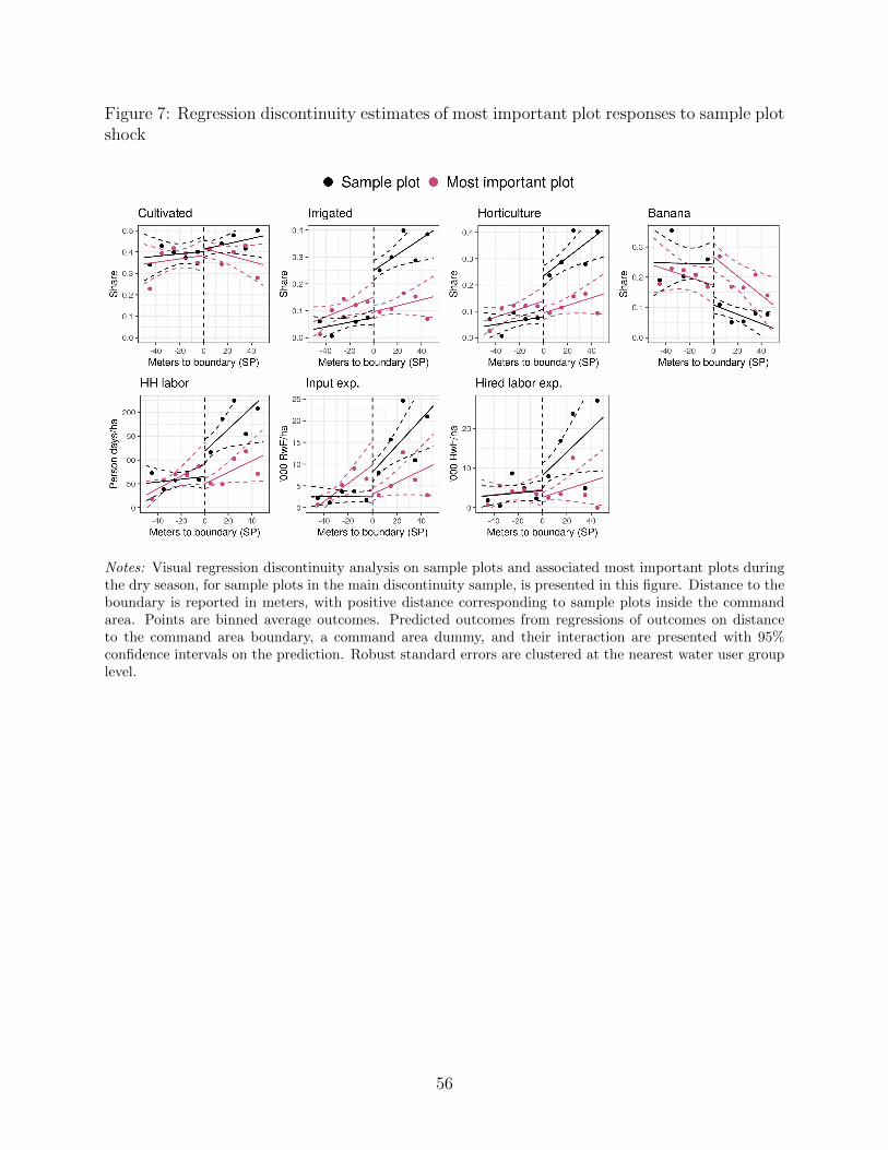
Figure 7: Regression discontinuity estimates of most important plot responses to sample plotshock

Notes: Visual regression discontinuity analysis on sample plots and associated most important plots duringthe dry season, for sample plots in the main discontinuity sample, is presented in this figure. Distance to theboundary is reported in meters, with positive distance corresponding to sample plots inside the commandarea. Points are binned average outcomes. Predicted outcomes from regressions of outcomes on distanceto the command area boundary, a command area dummy, and their interaction are presented with 95%confidence intervals on the prediction. Robust standard errors are clustered at the nearest water user grouplevel.

56

Table 1: Summary statistics on agricultural production

Staples Horticulture

Staples Maize Beans Bananas All Rainy Dry(1) (2) (3) (4) (5) (6) (7)

Yield 302 318 285 273 575 588 566Hired labor (days) 37 37 37 9 61 66 57HH labor (days) 266 248 260 101 417 414 420Inputs 19 35 16 3 50 50 50ProfitsShadow wage = 0 RwF/day 256 255 241 263 481 489 475Shadow wage = 800 RwF/day 43 56 34 182 147 158 139

Sales share 0.19 0.30 0.14 0.46 0.62 0.60 0.63Irrigated 0.02 0.02 0.02 0.02 0.65 0.25 0.93Rainy 0.99 1.00 1.00 0.50 0.42 1.00 0.00log area -2.44 -2.26 -2.47 -2.10 -2.71 -2.83 -2.62Share of obs. 0.65 0.13 0.42 0.19 0.12 0.05 0.07

Notes: Sample averages of outcomes by crop per agricultural season are presented in this table. Yield, inputs,and profits are reported in units of ’000 RwF/ha, labor variables are reported in units of person-days/ha,and log area is in units of log hectares. All other variables are shares or indicators. For reference, the medianwage in our data is 800 RwF/person-day.

57

Table 2: Balance: Sample plot characteristics

Full sample RD sample

Coef. (SE) [p] Dep. var. Coef. (SE) [p]

(1) (2) (3) (4) (5) (6) (7) (8)log area 0.045 -2.515 0.219 0.285 0.425 0.200

(0.077) (1.179) (0.087) (0.087) (0.121) (0.128)[0.554] 969 [0.012] [0.001] [0.000] [0.118]

Own plot -0.012 0.894 0.003 -0.001 0.004 -0.004 -0.001 -0.006(0.020) (0.309) (0.023) (0.024) (0.032) (0.038) (0.032) (0.038)[0.535] 969 [0.897] [0.966] [0.907] [0.921] [0.972] [0.877]

Owned plot >5 years 0.045 0.880 0.070 0.072 0.019 0.012 0.007 0.010(0.019) (0.326) (0.026) (0.025) (0.037) (0.035) (0.036) (0.034)[0.020] 686 [0.006] [0.004] [0.613] [0.723] [0.834] [0.767]

Rented out, farmer 0.027 0.032 0.018 0.019 -0.003 0.009 -0.009 0.007(0.012) (0.177) (0.014) (0.014) (0.023) (0.027) (0.023) (0.027)[0.022] 969 [0.197] [0.182] [0.884] [0.726] [0.699] [0.796]

Omnibus F-stat [p] 2.6 3.4 4.9 3.2 0.6 0.1 0.1[0.038] [0.010] [0.001] [0.013] [0.639] [0.979] [0.984]

Site FE X X XDistance to boundary X X X Xlog area X XSpatial FE X X

Notes: Balance for sample plot characteristics is presented in this table. Column 2 presents, for sample plotsin the main discontinuity sample that are outside the command area, the mean of the dependent variable, thestandard deviation of the dependent variable in parentheses, and the total number of observations. Columns1 and 3 through 8 present regression coefficients on a command area indicator, with standard errors inparentheses, and p-values in brackets. Robust standard errors are clustered at the nearest water user grouplevel in specifications without Spatial FE, and Conley (1999) standard errors are used in specifications withSpatial FE. Controls are listed below. The final row of each column presents the Omnibus F-stat for thenull of balance on all outcomes, with the p-value for the associated test in brackets. Column 1 uses the fullsample, while Columns 2 through 8 use the discontinuity sample. Column 4 uses the specification in Equation(1), Column 7 uses the specification in Equation (2), and Column 8 uses the specification in Equation (3).

58

Table 3: Balance: Household characteristics

Full sample RD sample

Coef. (SE) [p] Dep. var. Coef. (SE) [p]

(1) (2) (3) (4) (5) (6) (7) (8)HHH female 0.041 0.221 0.057 0.055 0.045 0.044 0.043 0.041

(0.025) (0.416) (0.029) (0.029) (0.046) (0.050) (0.046) (0.050)[0.094] 969 [0.054] [0.063] [0.326] [0.378] [0.345] [0.412]

HHH age 0.5 47.5 1.5 1.5 2.1 0.7 1.4 0.3(0.8) (14.5) (0.9) (0.9) (1.4) (1.8) (1.4) (1.9)

[0.497] 967 [0.096] [0.087] [0.127] [0.694] [0.298] [0.863]

HHH completed primary 0.069 0.287 0.044 0.052 0.128 0.102 0.119 0.099(0.025) (0.453) (0.031) (0.032) (0.047) (0.062) (0.047) (0.062)[0.005] 966 [0.159] [0.106] [0.006] [0.097] [0.012] [0.111]

HHH worked off farm 0.023 0.410 -0.023 -0.033 -0.039 -0.019 -0.024 -0.011(0.027) (0.493) (0.035) (0.035) (0.051) (0.064) (0.050) (0.064)[0.392] 969 [0.516] [0.350] [0.441] [0.763] [0.631] [0.868]

# of plots 0.61 5.19 0.37 0.16 0.20 0.35 0.36 0.40(0.18) (3.38) (0.22) (0.21) (0.36) (0.46) (0.36) (0.46)[0.001] 969 [0.099] [0.442] [0.582] [0.448] [0.319] [0.382]

# of HH members 0.17 4.89 0.04 0.02 -0.00 -0.03 -0.01 -0.03(0.11) (2.16) (0.15) (0.15) (0.21) (0.25) (0.22) (0.25)[0.104] 969 [0.799] [0.916] [0.985] [0.917] [0.971] [0.908]

# who worked off farm 0.10 0.77 0.04 0.02 0.01 0.03 0.01 0.04(0.05) (0.85) (0.06) (0.06) (0.08) (0.10) (0.08) (0.10)[0.039] 969 [0.523] [0.771] [0.909] [0.799] [0.906] [0.722]

Housing expenditures -2.3 49.2 3.5 3.3 -5.6 -16.7 -6.5 -18.6(6.9) (127.4) (9.0) (9.0) (14.9) (19.0) (14.7) (19.1)

[0.739] 962 [0.700] [0.717] [0.707] [0.380] [0.658] [0.328]

Asset index 0.11 -0.12 0.06 0.07 0.15 0.06 0.13 0.04(0.05) (0.99) (0.07) (0.07) (0.12) (0.13) (0.12) (0.13)[0.034] 967 [0.372] [0.303] [0.215] [0.647] [0.291] [0.738]

Omnibus F-stat [p] 3.6 1.6 1.6 1.8 0.8 1.5 0.9[0.000] [0.122] [0.118] [0.080] [0.571] [0.158] [0.507]

Site FE X X XDistance to boundary X X X Xlog area X XSpatial FE X X

Notes: Balance for household characteristics is presented in this table. Column 2 presents, for sample plotsin the main discontinuity sample that are outside the command area, the mean of the dependent variable, thestandard deviation of the dependent variable in parentheses, and the total number of observations. Columns1 and 3 through 8 present regression coefficients on a command area indicator, with standard errors inparentheses, and p-values in brackets. Robust standard errors are clustered at the nearest water user grouplevel in specifications without Spatial FE, and Conley (1999) standard errors are used in specifications withSpatial FE. Controls are listed below. The final row of each column presents the Omnibus F-stat for thenull of balance on all outcomes, with the p-value for the associated test in brackets. Column 1 uses the fullsample, while Columns 2 through 8 use the discontinuity sample. Column 4 uses the specification in Equation(1), Column 7 uses the specification in Equation (2), and Column 8 uses the specification in Equation (3).

59

Table 4: Access to irrigation enables transition to dry season horticulture from perennialbananas

Dry season Rainy seasons

Dep. var. Coef. (SE) [p] Dep. var. Coef. (SE) [p]

(1) (2) (3) (4) (5) (6) (7) (8)Cultivated 0.391 0.033 0.005 0.022 0.838 -0.054 -0.092 -0.053

(0.488) (0.031) (0.041) (0.044) (0.369) (0.020) (0.025) (0.027)2,537 [0.289] [0.909] [0.610] 4,236 [0.006] [0.000] [0.051]

Irrigated 0.058 0.202 0.162 0.171 0.016 0.044 0.035 0.059(0.233) (0.019) (0.024) (0.030) (0.127) (0.007) (0.009) (0.012)2,537 [0.000] [0.000] [0.000] 4,236 [0.000] [0.000] [0.000]

Horticulture 0.065 0.180 0.137 0.156 0.073 0.044 0.016 0.048(0.246) (0.020) (0.024) (0.029) (0.260) (0.011) (0.018) (0.025)2,536 [0.000] [0.000] [0.000] 4,235 [0.000] [0.371] [0.056]

Banana 0.245 -0.134 -0.133 -0.142 0.274 -0.149 -0.158 -0.168(0.430) (0.024) (0.037) (0.035) (0.446) (0.024) (0.038) (0.034)2,536 [0.000] [0.000] [0.000] 4,235 [0.000] [0.000] [0.000]

Site-by-season FE X X X XDistance to boundary X X X Xlog area X X X XSpatial FE X X

Notes: Regression analysis is presented in this table. Columns 1 through 4 restrict to observations duringthe dry season, while columns 5 through 8 restrict to observations during the rainy season. Columns 1and 5 present, for sample plots in the main discontinuity sample that are outside the command area, themean of the dependent variable, the standard deviation of the dependent variable in parentheses, and thetotal number of observations. Columns 2 through 4 and 6 through 8 present regression coefficients on acommand area indicator, with standard errors in parentheses, and p-values in brackets. Robust standarderrors are clustered at the nearest water user group level in specifications without Spatial FE, and Conley(1999) standard errors are used in specifications with Spatial FE. Columns 2 and 6 use the specification inEquation (1). Columns 3 and 7 use the regression discontinuity specification in Equation (2). Columns 4and 8 use the spatial fixed effects specification in Equation (3).

60

Table 5: Access to irrigation causes large increases in dry season labor and input use

Dry season Rainy seasons

Dep. var. Coef. (SE) [p] Dep. var. Coef. (SE) [p]

(1) (2) (3) (4) (5) (6) (7) (8)HH labor/ha 59.5 69.6 70.8 76.9 226.7 -7.7 8.5 9.9

(201.4) (14.7) (17.5) (20.7) (316.7) (18.3) (23.1) (24.7)2,523 [0.000] [0.000] [0.000] 4,215 [0.671] [0.714] [0.689]

Input exp./ha 2.5 7.4 6.3 4.3 16.1 2.5 1.1 2.1(17.4) (1.3) (1.5) (1.8) (40.9) (2.0) (2.9) (3.1)2,527 [0.000] [0.000] [0.019] 4,223 [0.205] [0.710] [0.511]

Hired labor exp./ha 3.7 5.6 3.7 3.2 15.9 7.1 3.7 3.1(25.6) (1.9) (2.1) (2.6) (47.1) (2.4) (3.4) (4.5)2,527 [0.003] [0.082] [0.221] 4,223 [0.003] [0.276] [0.490]

Site-by-season FE X X X XDistance to boundary X X X Xlog area X X X XSpatial FE X X

Notes: Regression analysis is presented in this table. Columns 1 through 4 restrict to observations duringthe dry season, while columns 5 through 8 restrict to observations during the rainy season. Columns 1and 5 present, for sample plots in the main discontinuity sample that are outside the command area, themean of the dependent variable, the standard deviation of the dependent variable in parentheses, and thetotal number of observations. Columns 2 through 4 and 6 through 8 present regression coefficients on acommand area indicator, with standard errors in parentheses, and p-values in brackets. Robust standarderrors are clustered at the nearest water user group level in specifications without Spatial FE, and Conley(1999) standard errors are used in specifications with Spatial FE. Columns 2 and 6 use the specification inEquation (1). Columns 3 and 7 use the regression discontinuity specification in Equation (2). Columns 4and 8 use the spatial fixed effects specification in Equation (3).

61

Table 6: Access to irrigation causes large increases in dry season yields and sales, profitabilitydepends on household’s shadow wage

Dry season Rainy seasons

Dep. var. Coef. (SE) [p] Dep. var. Coef. (SE) [p]

(1) (2) (3) (4) (5) (6) (7) (8)Yield 82.3 61.2 73.1 55.0 271.5 -45.1 -22.6 -15.4

(278.7) (20.7) (23.2) (28.5) (457.0) (22.0) (30.8) (30.8)2,402 [0.003] [0.002] [0.054] 4,085 [0.041] [0.462] [0.617]

Sales/ha 49.7 52.3 55.5 49.3 85.1 -4.8 -13.3 5.6(180.8) (13.3) (14.5) (19.2) (229.1) (10.8) (18.5) (21.6)2,527 [0.000] [0.000] [0.010] 4,223 [0.660] [0.472] [0.793]

Profits/ha

Shadow wage = 0 76.1 49.6 63.9 49.1 239.8 -53.4 -26.4 -19.4(265.9) (18.6) (21.0) (25.7) (432.5) (20.5) (28.5) (27.5)2,402 [0.008] [0.002] [0.057] 4,085 [0.009] [0.354] [0.480]

Shadow wage = 800 32.8 -0.3 9.3 -3.0 59.5 -47.2 -31.8 -27.3(224.1) (12.0) (16.5) (20.8) (364.5) (16.5) (26.4) (31.9)2,400 [0.978] [0.573] [0.886] 4,078 [0.004] [0.228] [0.393]

Site-by-season FE X X X XDistance to boundary X X X Xlog area X X X XSpatial FE X X

Notes: Regression analysis is presented in this table. Columns 1 through 4 restrict to observations duringthe dry season, while columns 5 through 8 restrict to observations during the rainy season. Columns 1and 5 present, for sample plots in the main discontinuity sample that are outside the command area, themean of the dependent variable, the standard deviation of the dependent variable in parentheses, and thetotal number of observations. Columns 2 through 4 and 6 through 8 present regression coefficients on acommand area indicator, with standard errors in parentheses, and p-values in brackets. Robust standarderrors are clustered at the nearest water user group level in specifications without Spatial FE, and Conley(1999) standard errors are used in specifications with Spatial FE. Columns 2 and 6 use the specification inEquation (1). Columns 3 and 7 use the regression discontinuity specification in Equation (2). Columns 4and 8 use the spatial fixed effects specification in Equation (3).

62

Table 7: Model predictions

dL2

dA1

d

dL

dL2

dA1

d

dM

dL2

dA1

No constraints 0 0 0

Constraints

Insurance − + +Inputs − 0/+ +Labor − +∗ −∗

Notes: Predicted signs from the model for key comparative statics of interest are presented in this table. Pre-dictions in the no constraints case correspond to Proposition 1. Predictions on dL2

dA1correspond to Proposition

2. Predictions on ddL

dL2

dA1and d

dMdL2

dA1when insurance or input constraints bind correspond to Proposition

3, and when labor constraints bind correspond to Proposition 4. * is used to indicate predictions that holdwhen additional assumptions are made.

63

Table 8: Balance: Most important plot characteristics

Full sample RD sample

Coef. (SE) [p] Dep. var. Coef. (SE) [p]

(1) (2) (3) (4) (5) (6) (7) (8)log area -0.108 -2.381 0.043 0.089 0.094 0.074

(0.068) (1.041) (0.083) (0.082) (0.128) (0.136)[0.114] 784 [0.603] [0.275] [0.460] [0.588]

Own plot 0.025 0.875 0.048 0.043 0.040 0.033 0.039 0.029(0.019) (0.331) (0.023) (0.023) (0.033) (0.039) (0.032) (0.037)[0.174] 784 [0.037] [0.064] [0.226] [0.392] [0.232] [0.436]

Owned plot >5 years 0.005 0.960 -0.004 -0.003 0.012 0.033 0.011 0.030(0.014) (0.197) (0.016) (0.016) (0.024) (0.024) (0.023) (0.025)[0.728] 585 [0.811] [0.853] [0.617] [0.175] [0.617] [0.233]

Rented out, farmer 0.013 0.033 -0.006 -0.006 -0.026 -0.040 -0.029 -0.041(0.010) (0.179) (0.013) (0.013) (0.022) (0.025) (0.023) (0.026)[0.224] 784 [0.664] [0.645] [0.249] [0.114] [0.222] [0.116]

Command area 0.187 0.399 0.074 0.045 -0.053 -0.079(0.032) (0.491) (0.039) (0.037) (0.058) (0.059)[0.000] 784 [0.059] [0.219] [0.360] [0.183]

Terraced 0.017 0.626 -0.030 -0.043 -0.099 -0.091 -0.076 -0.058(0.028) (0.485) (0.035) (0.035) (0.053) (0.055) (0.051) (0.052)[0.539] 784 [0.403] [0.225] [0.063] [0.099] [0.134] [0.260]

Rented out, comm. farmer 0.035 0.081 0.017 0.008 -0.042 -0.016 -0.036 -0.004(0.018) (0.273) (0.025) (0.023) (0.040) (0.034) (0.036) (0.031)[0.054] 784 [0.486] [0.735] [0.292] [0.638] [0.324] [0.895]

Omnibus F-stat [p] 5.6 1.8 1.6 1.3 1.5 1.4 1.2[0.000] [0.093] [0.132] [0.278] [0.153] [0.209] [0.292]

Site FE X X XDistance to boundary X X X Xlog area X XMIP log area X XMIP CA X XSpatial FE X X

Notes: Balance for most important plot characteristics is presented in this table. Column 2 presents,for sample plots in the main discontinuity sample that are outside the command area, the mean of thedependent variable, the standard deviation of the dependent variable in parentheses, and the total numberof observations. Columns 1 and 3 through 8 present regression coefficients on a command area indicator,with standard errors in parentheses, and p-values in brackets. Robust standard errors are clustered at thenearest water user group level in specifications without Spatial FE, and Conley (1999) standard errors areused in specifications with Spatial FE. Controls are listed below. The final row of each column presents theOmnibus F-stat for the null of balance on all outcomes, with the p-value for the associated test in brackets.Column 1 uses the full sample, while Columns 2 through 8 use the discontinuity sample. Column 4 usesthe specification in Equation (7), Column 7 uses the specification in Equation (8), and Column 8 uses thespecification in Equation (9).

64

Table 9: Sample plot shock causes households to substitute labor and input intensive irri-gated horticulture away from most important plot

Sample plot MIP

Coef. (SE) [p] Dep. var. Coef. (SE) [p]

(1) (2) (3) (4) (5) (6) (7) (8)Cultivated

CA 0.033 0.368 0.049 0.038 0.004 0.085 0.076 0.059(0.031) (0.483) (0.023) (0.040) (0.049) (0.030) (0.043) (0.048)[0.289] 2,179 [0.035] [0.344] [0.930] [0.005] [0.079] [0.215]

CA * MIP CA -0.094 -0.089 -0.121(0.053) (0.052) (0.056)[0.078] [0.089] [0.030]

Joint F-stat [p] 3.9 2.1 2.7[0.021] [0.122] [0.070]

Irrigated

CA 0.202 0.114 -0.019 -0.044 -0.036 0.013 -0.004 0.010(0.019) (0.319) (0.017) (0.026) (0.033) (0.008) (0.020) (0.026)[0.000] 2,179 [0.251] [0.087] [0.270] [0.123] [0.836] [0.686]

CA * MIP CA -0.097 -0.094 -0.103(0.035) (0.035) (0.045)[0.006] [0.007] [0.021]

Joint F-stat [p] 4.1 3.6 2.7[0.019] [0.028] [0.069]

Site-by-season FE X X X X XDistance to boundary X X X Xlog area X X X XSpatial FE X XMIP log area X X X XMIP CA X X X X X

Notes: Regression analysis is presented in this table. Column 1 uses outcomes on the sample plot (andreplicates analysis in Table 4), while Columns 3 through 8 use outcomes on the associated most importantplot. All columns restrict to observations during the dry season. Column 2 presents, for the most importantplot associated with sample plots in the main discontinuity sample that are outside the command area, themean of the dependent variable, the standard deviation of the dependent variable in parentheses, and thetotal number of observations. For Columns 1 and 3 through 8, Rows “CA” present coefficients on a commandarea indicator for the sample plot, while Rows “CA * MIP in CA” present coefficients on the interaction ofa command area indicator for the sample plot with a command area indicator for the most important plot;standard errors are in parentheses, and p-values are in brackets. Robust standard errors are clustered atthe nearest water user group level in specifications without Spatial FE, and Conley (1999) standard errorsare used in specifications with Spatial FE. Column 3 uses the specification in Equation (7), Column 4 usesthe specification in Equation (8), and Column 5 uses the specification in Equation (9). Columns 6 though 8uses analogous specifications building on Equation (10).

65

Table 10: Sample plot shock causes households to substitute labor and input intensiveirrigated horticulture away from most important plot

Sample plot MIP

Coef. (SE) [p] Dep. var. Coef. (SE) [p]

(1) (2) (3) (4) (5) (6) (7) (8)Horticulture

CA 0.180 0.109 -0.016 -0.038 -0.037 0.010 -0.004 -0.007(0.020) (0.312) (0.016) (0.024) (0.029) (0.009) (0.018) (0.023)[0.000] 2,179 [0.323] [0.110] [0.206] [0.244] [0.813] [0.771]

CA * MIP CA -0.082 -0.080 -0.066(0.035) (0.035) (0.044)[0.020] [0.021] [0.133]

Joint F-stat [p] 2.9 2.7 1.3[0.060] [0.070] [0.286]

Banana

CA -0.134 0.199 0.066 0.092 0.065 0.077 0.096 0.087(0.024) (0.399) (0.023) (0.032) (0.036) (0.033) (0.041) (0.044)[0.000] 2,179 [0.004] [0.004] [0.072] [0.021] [0.019] [0.047]

CA * MIP CA -0.013 -0.009 -0.048(0.043) (0.042) (0.044)[0.766] [0.824] [0.275]

Joint F-stat [p] 5.9 4.5 2.0[0.003] [0.013] [0.139]

Site-by-season FE X X X X XDistance to boundary X X X Xlog area X X X XSpatial FE X XMIP log area X X X XMIP CA X X X X X

Notes: Regression analysis is presented in this table. Column 1 uses outcomes on the sample plot (andreplicates analysis in Table 4), while Columns 3 through 8 use outcomes on the associated most importantplot. All columns restrict to observations during the dry season. Column 2 presents, for the most importantplot associated with sample plots in the main discontinuity sample that are outside the command area, themean of the dependent variable, the standard deviation of the dependent variable in parentheses, and thetotal number of observations. For Columns 1 and 3 through 8, Rows “CA” present coefficients on a commandarea indicator for the sample plot, while Rows “CA * MIP in CA” present coefficients on the interaction ofa command area indicator for the sample plot with a command area indicator for the most important plot;standard errors are in parentheses, and p-values are in brackets. Robust standard errors are clustered atthe nearest water user group level in specifications without Spatial FE, and Conley (1999) standard errorsare used in specifications with Spatial FE. Column 3 uses the specification in Equation (7), Column 4 usesthe specification in Equation (8), and Column 5 uses the specification in Equation (9). Columns 6 though 8uses analogous specifications building on Equation (10).

66

Table 11: Sample plot shock causes households to substitute labor and input intensiveirrigated horticulture away from most important plot

Sample plot MIP

Coef. (SE) [p] Dep. var. Coef. (SE) [p]

(1) (2) (3) (4) (5) (6) (7) (8)HH labor/ha

CA 69.6 66.8 -11.2 -32.2 -33.2 3.2 -13.6 -15.4(14.7) (210.5) (11.9) (20.0) (23.8) (6.2) (14.1) (19.2)[0.000] 2,166 [0.351] [0.107] [0.162] [0.609] [0.338] [0.422]

CA * MIP CA -41.7 -44.1 -39.7(26.8) (23.5) (31.2)[0.120] [0.060] [0.204]

Joint F-stat [p] 1.2 1.8 1.1[0.290] [0.164] [0.324]

Input exp./ha

CA 7.4 5.6 -2.1 -6.0 -6.7 0.2 -3.3 -3.8(1.3) (28.2) (1.5) (2.7) (2.8) (0.7) (1.8) (2.1)

[0.000] 2,169 [0.158] [0.028] [0.017] [0.805] [0.070] [0.076]

CA * MIP CA -6.3 -6.3 -6.5(3.4) (3.2) (3.7)

[0.067] [0.044] [0.079]

Joint F-stat [p] 1.7 2.6 3.0[0.190] [0.078] [0.050]

Hired labor exp./ha

CA 5.6 3.9 -0.9 -1.8 -0.5 0.8 0.2 1.5(1.9) (24.6) (1.3) (2.1) (2.3) (1.2) (2.1) (2.6)

[0.003] 2,169 [0.506] [0.404] [0.825] [0.477] [0.922] [0.546]

CA * MIP CA -4.4 -4.7 -4.5(2.7) (2.5) (3.1)

[0.099] [0.066] [0.146]

Joint F-stat [p] 1.4 1.8 1.1[0.255] [0.175] [0.345]

Site-by-season FE X X X X XDistance to boundary X X X Xlog area X X X XSpatial FE X XMIP log area X X X XMIP CA X X X X X

Notes: Regression analysis is presented in this table. Column 1 uses outcomes on the sample plot (andreplicates analysis in Table 5), while Columns 3 through 8 use outcomes on the associated most importantplot. All columns restrict to observations during the dry season. Column 2 presents, for the most importantplot associated with sample plots in the main discontinuity sample that are outside the command area, themean of the dependent variable, the standard deviation of the dependent variable in parentheses, and thetotal number of observations. For Columns 1 and 3 through 8, Rows “CA” present coefficients on a commandarea indicator for the sample plot, while Rows “CA * MIP in CA” present coefficients on the interaction ofa command area indicator for the sample plot with a command area indicator for the most important plot;standard errors are in parentheses, and p-values are in brackets. Robust standard errors are clustered atthe nearest water user group level in specifications without Spatial FE, and Conley (1999) standard errorsare used in specifications with Spatial FE. Column 3 uses the specification in Equation (7), Column 4 usesthe specification in Equation (8), and Column 5 uses the specification in Equation (9). Columns 6 though 8uses analogous specifications building on Equation (10).

67

Table 12: Larger and poorer households do not substitute away from most important plotin response to sample plot shock

MIP

Coef. (SE) [p]

(1) (2) (3)Cultivated

CA -0.046 -0.069 -0.188(0.073) (0.086) (0.098)[0.526] [0.424] [0.056]

CA * # of HH members 0.019 0.021 0.039(0.013) (0.013) (0.014)[0.158] [0.112] [0.007]

CA * Asset index -0.007 -0.013 -0.043(0.028) (0.027) (0.032)[0.814] [0.620] [0.181]

Joint F-stat [p] 2.4 1.5 3.5[0.072] [0.213] [0.015]

Irrigated

CA -0.071 -0.097 -0.121(0.043) (0.048) (0.051)[0.098] [0.046] [0.017]

CA * # of HH members 0.010 0.011 0.017(0.009) (0.007) (0.008)[0.227] [0.155] [0.030]

CA * Asset index -0.022 -0.018 -0.035(0.020) (0.016) (0.020)[0.256] [0.277] [0.077]

Joint F-stat [p] 1.3 1.5 2.3[0.284] [0.214] [0.079]

# of HH members X X XAsset index X X XSite-by-season FE X XDistance to boundary X Xlog area X XMIP log area X XMIP CA X XSpatial FE X

MIP

Coef. (SE) [p]

(1) (2) (3)Horticulture

CA -0.082 -0.107 -0.129(0.041) (0.046) (0.047)[0.045] [0.020] [0.006]

CA * # of HH members 0.013 0.014 0.019(0.008) (0.007) (0.007)[0.109] [0.061] [0.012]

CA * Asset index -0.019 -0.015 -0.030(0.020) (0.017) (0.021)[0.353] [0.384] [0.156]

Joint F-stat [p] 1.5 1.8 2.6[0.225] [0.147] [0.050]

Banana

CA 0.036 0.052 -0.052(0.064) (0.065) (0.083)[0.573] [0.418] [0.532]

CA * # of HH members 0.006 0.008 0.023(0.011) (0.011) (0.015)[0.596] [0.485] [0.110]

CA * Asset index 0.009 -0.003 -0.012(0.024) (0.023) (0.026)[0.696] [0.900] [0.661]

Joint F-stat [p] 3.0 3.1 2.1[0.031] [0.026] [0.094]

# of HH members X X XAsset index X X XSite-by-season FE X XDistance to boundary X Xlog area X XMIP log area X XMIP CA X XSpatial FE X

Notes: Regression analysis is presented in this table. All columns use outcomes on most important plotsand restrict to observations during the dry season.. Rows “CA” present coefficients on a command areaindicator for the sample plot, while Rows “CA * W” present coefficients on the interaction of a commandarea indicator for the sample plot with a household characteristic W; standard errors are in parentheses,and p-values are in brackets. Robust standard errors are clustered at the nearest water user group level inspecifications without Spatial FE, and Conley (1999) standard errors are used in specifications with SpatialFE. The Row “Joint F-stat [p]” presents F-statistics for the null that all 3 coefficients are 0, with the p-valuefor the associated test in brackets. Columns 1, 2, and 3 use regression specifications building on Equation(10) following Equations (7), (8), and (9), respectively.

68

Table 13: Larger and poorer households do not substitute away from most important plotin response to sample plot shock

MIP

Coef. (SE) [p]

(1) (2) (3)HH labor/ha

CA -78.5 -82.7 -94.6(32.0) (34.8) (38.9)[0.014] [0.018] [0.015]

CA * # of HH members 13.4 10.1 12.5(5.5) (4.5) (4.5)

[0.015] [0.025] [0.006]

CA * Asset index -22.7 -12.4 -24.0(12.7) (10.2) (12.7)[0.074] [0.226] [0.060]

Joint F-stat [p] 2.1 2.0 2.9[0.099] [0.122] [0.033]

Input exp./ha

CA -6.2 -9.1 -10.3(3.5) (4.2) (4.1)

[0.075] [0.031] [0.013]

CA * # of HH members 0.8 0.6 0.7(0.6) (0.5) (0.5)

[0.161] [0.237] [0.185]

CA * Asset index -3.2 -2.5 -3.9(1.8) (1.6) (1.7)

[0.076] [0.117] [0.025]

Joint F-stat [p] 1.4 1.9 2.6[0.239] [0.128] [0.051]

# of HH members X X XAsset index X X XSite-by-season FE X XDistance to boundary X Xlog area X XMIP log area X XMIP CA X XSpatial FE X

MIP

Coef. (SE) [p]

(1) (2) (3)Hired labor exp./ha

CA -4.1 -4.5 -2.1(2.9) (3.6) (3.5)

[0.155] [0.216] [0.551]

CA * # of HH members 0.6 0.5 0.3(0.5) (0.5) (0.5)

[0.201] [0.273] [0.539]

CA * Asset index -0.1 0.3 -0.3(1.4) (1.4) (1.4)

[0.968] [0.856] [0.813]

Joint F-stat [p] 0.8 0.6 0.1[0.488] [0.592] [0.937]

# of HH members X X XAsset index X X XSite-by-season FE X XDistance to boundary X Xlog area X XMIP log area X XMIP CA X XSpatial FE X

Notes: Regression analysis is presented in this table. All columns use outcomes on most important plotsand restrict to observations during the dry season.. Rows “CA” present coefficients on a command areaindicator for the sample plot, while Rows “CA * W” present coefficients on the interaction of a commandarea indicator for the sample plot with a household characteristic W; standard errors are in parentheses,and p-values are in brackets. Robust standard errors are clustered at the nearest water user group level inspecifications without Spatial FE, and Conley (1999) standard errors are used in specifications with SpatialFE. The Row “Joint F-stat [p]” presents F-statistics for the null that all 3 coefficients are 0, with the p-valuefor the associated test in brackets. Columns 1, 2, and 3 use regression specifications building on Equation(10) following Equations (7), (8), and (9), respectively.

69

Table 14: Minikits do not cause increased adoption of horticulture, strong positive selectioninto minikit takeup

Minikit takeup Horticulture

(1) (2) (3) (4)Assigned minikit 0.398 0.395 0.035 0.052

(0.038) (0.044) (0.041) (0.042)[0.000] [0.000] [0.396] [0.221]

Minikit saturation -0.047 -0.064 -0.078 -0.067(0.056) (0.057) (0.054) (0.054)[0.394] [0.260] [0.149] [0.218]

Horticulture (2016 Dry) 0.046 0.306(0.049) (0.053)[0.345] [0.000]

Assigned minikit * Horticulture (2016 Dry) 0.131 -0.019(0.068) (0.070)[0.052] [0.788]

# of lotteries entered X X X XO&M treatment X X X XZone FE X X X X# of observations 910 762 838 727# of clusters 187 170 182 167

Notes: Regression analysis is presented in this table. All columns use outcomes on sample plots. Each rowpresents coefficients, with robust standard errors clustered at the water user group level in parentheses, andp-values in brackets. “Assigned minikit” is an indicator for whether the household was assigned to receivea minikit, “Minikit saturation” is the probability of minikit assignment that was assigned to the water usergroup of the household’s sample plot, and “Horticulture (2016 Dry)” is an indicator that the householdplanted horticulture on their sample plot in 2016 Dry.

70

A Main variable appendix

Household variables: All household variables are constructed from the baseline.

• HHH female: Indicator that the household head is female.

• HHH age: Age of the household head.

• HHH completed primary : Indicator that the household head completed primary.

• HHH worked off farm: Indicator that the household head worked off farm.

• # of plots : Number of plots reported as managed by the household. Includes plots

rented in, plots owned and cultivated in the past year, and plots rented out.

• # of HH members : Number of members of the household.

• # of HH members who worked off farm: Number of members of the household who

worked off farm.

• Housing expenditures : Expenditures over the past year on housing and furnishing.

Winsorized at the 99th percentile.

• Asset index : First principal component of log number of assets-by-category owned and

an indicator for positive number of assets-by-category owned, where the categories are

cows, goats, pigs, chickens, radios, mobile phones, pieces of furniture, bicycles, and

shovels. Standardized to be mean 0 and standard deviation 1, with positive values

indicating more assets.

• Food security index : First principal component of log days in the past week of con-

sumption of food item-by-category and an indicator for any consumption of food item-

by-category. In baseline, categories are flour, bread, rice, meat and fish, poultry and

eggs, dairy products, cooking oil, fruits, beans, vegetables, plantains and cassava and

potatoes, juice and soda, sugar and honey, salt and spices, meals prepared outside

71

home, and groundnut and other oilseed flour. In follow up surveys, categories are

flour, bread, cakes and chapati and mandazi, rice, small fish, meats and other fish,

poultry and eggs, dairy products, peanut oil, palm oil and other cooking oil, avocados,

other fruits, beans, tomato, onion, other vegetables, plantains, Irish potatoes, sweet

potatoes, sugar, salt, local banana beer at home, groundnut flour. Standardized to be

mean 0 and standard deviation 1, with positive values indicating more consumption.

• Overall index : Index constructed following Anderson (2008) using housing expendi-

tures, asset index, and food security index.

Plot variables: All plot variables are constructed from the baseline.

• Command area: Indicator that plot located in command area, equal 1 if any share of

the plot is inside of the command area. Calculated from plot map.

• Distance to boundary : Distance from plot boundary to command area boundary, 0 for

plots whose plot map intersects the boundary. Positive for plots that are inside the

command area, negative for plots that are outside the command area. Calculated from

plot map.

• Area: Area in hectares. Calculated from plot map.

• Water user group: Water user groups that the plot is located in, calculated from plot

map. If the plot intersects multiple water user group boundaries, the water user group

in which the largest share of the plot’s area is contained. Missing for plots that are

outside the command area.

• Nearest water user group: For plots inside the command area, the water user group. For

plots outside the command area, the water user group whose boundary the boundary

of the plot is the shortest distance from. Calculated from plot map.

• Terraced : Indicator that the plot was terraced.

72

Plot-season variables: All plot-season variables are constructed from the baseline when

used in balance tables. Variables related to attrition are observed at plot-season level when

used as outcomes in regressions testing for differential attrition.

• Own plot : Indicator that the surveyed cultivator owns the plot. 0 when the surveyed

cultivator rents in the plot.

• Owned plot >5 years : Indicator that the surveyed cultivator had owned the plot for

at least 5 years.

• Rented out to farmer : Indicator that the surveyed cultivator rented out the plot to

another farmer.

• Rented out to commercial farmer : Indicator that the plot was rented out to a com-

mercial farmer.

• HH attrition: Plot-season indicator that the household associated with the plot was

not reached for the survey.

• Transaction (not tracked): Plot-season indicator that the plot was sold, rented out, or

no longer rented in, and the new household responsible for the plot was not successfully

followed up with.

• Tracked : Plot-season indicator that the plot was sold, rented out, or no longer rented

in, and the new household responsible for the plot was successfully followed up with

and asked questions on agricultural production on the plot.

• Missing : Plot-season indicator that agricultural production data is missing for that

plot. Sum of variables HH attrition, Rented out to commercial farmer, and Transaction

(not tracked).

Agricultural variables

73

• Cultivated : Plot-season indicator for any cultivation. All other agricultural variables

are set to 0 when no cultivation takes place.

• Irrigated : Plot-season indicator for any irrigation use.

• Horticulture: Plot-season indicator for any horticulture cultivated. As horticultural

crops are annuals, this will include activities associated with planting, growing, and

harvesting.54

• Banana: Plot-season indicator for any bananas cultivated. As bananas are perennials,

this refers to any activities associated with planting, growing, or harvesting, and need

not include all three.

• HH labor/ha: Plot-season sum of household labor use, divided by plot area. Winsorized

at the 99th percentile.

• Input expenditures/ha: Plot-season sum of expenditures on non-labor inputs, divided

by plot area. Winsorized at the 99th percentile.

• Hired labor expenditures/ha: Plot-season sum of expenditures on hired labor, divided

by plot area. Winsorized at the 99th percentile.

• Hired labor (days)/ha: Plot-season sum of hired labor use, divided by plot area. Win-

sorized at the 99th percentile.

• Price: Prices are calculated at the District-crop-season level, as the median of plot-

crop-season reported sales divided by reported kilograms sold. Prices are set to missing

when there are less than 10 observations that District-crop-season and either more

than two District-crop-seasons with at least 10 observations that District-crop-survey

or at least 30 observations that District-crop-survey; these cut-off points were chosen

54In Figure 3 and Table 1, an alternative definition of crop choice is used, where a crop indicator indicatesthat crop is the primary crop cultivated that plot-season.

74

to maximize inclusion of prices judged subjectively to be reasonable, and maximize

exclusion of prices judged subjectively to be not reasonable.

• Yield : Plot-season sum of prices times harvested quantities. Yields are missing when

all crops cultivated that plot-season have missing prices or missing harvested quanti-

ties. When multiple crops are grown on a plot-season and some have observed prices

and harvested quantities, those with missing prices or quantities are treated as 0 pro-

duction. After this procedure 3.6% of rainy season observations and 5.3% of dry season

observations in our discontinuity sample have missing yields. Winsorized at the 99th

percentile.

• Sales/ha: Plot-season total reported sales, divided by area. Winsorized at the 99th

percentile.

• Sales share: Sales/ha divided by yield, equal to 1 when reported sales/ha is greater

than yield.

• Profits/ha (Shadow wage = 0 RwF/day): Yield minus hired labor expenditures/ha

minus input expenditures/ha.

• Profits/ha (Shadow wage = 800 RwF/day): Yield minus hired labor expenditures/ha

minus input expenditures/ha minus 800 times HH labor/ha.

Experimental variables: Additional details on these variables are in Appendix E.

• Assigned minikit : Indicator that household was assigned to receive a minikit.

• Minikit saturation: Saturation of minikits assigned for the Water User Group of the

plot.

• Minikit takeup: Indicator that the household reported using a minikit.

• Zone: The Zone in which the plot’s Water User Group is located in. The plots in our

survey are located in 239 Water User Groups grouped into 33 Zones.

75

• O&M treatment : O&M treatment status of the Water User Group of the plot.

• # of lotteries entered, minikits : Number of lotteries for minikits the household was

entered into.

B Household results

We present results of the impacts of access to irrigation on household welfare outcomes in

Table A3. We estimate specifications similar to Equations (1), (2), and (3), but now use

annual outcomes at the household level (instead of outcomes on sample plots).

We find suggestive evidence of positive impacts on household welfare. All point esti-

mates are positive, and impacts on housing expenditures and an Anderson (2008) index of

household welfare are each significantly different from zero in two specifications. The im-

plied treatment on the treated estimates are large. However, as impacts on household are

imprecisely estimated, we interpret these results with caution.

C Prices and wages

We present figures showing the evolution of wages (Figure A1) and sale prices (Figure A2)

across the 3 hillside irrigation schemes. In Figure A1, average wages do not appear to change

after the hillside irrigation schemes became fully operational.55 In Figure A2, median sale

prices appear to display more meaningful trends. In Karongi, there do not appear to be any

trends in sale prices of horticultural crops. However, in Nyanza, sale prices of both tomatoes

and eggplants appear lower after the hillside irrigation schemes became fully operational

than before. We discuss the interpretation of these changes, if one believes they are causal,

in Section 3.2.3.

55Median wages (not presented here) remain constant within both of the sites used for the regressiondiscontinuity analysis, and are slightly higher in the third site after the hillside irrigation schemes becamefully operational.

76

D Model appendix

Derivation of first order conditions. Substitute for LO using the household labor con-

straint, L1 +L2 + `+LO = L, and substitute for c in the household’s maximization problem.

This leaves two constraints, M1 +M2 ≤ M , and L− L1 − L2 − ` ≤ LO; call the multipliers

on these constraints λ̃M and λ̃L, respectively. Taking first order conditions yields

(Mk) E[ucσ]AkFkM − E[uc]r = λ̃M

(Lk) E[ucσ]AkFkL − E[uc]w = −λ̃L

(`) E[u`]− E[uc]w = −λ̃L

To ease interpretation, normalize λM ≡ λ̃M/rE[uc] and λL ≡ λ̃L/wE[uc], and substitute

cov(σ, uc) = E[ucσ]− E[uc]E[σ] = E[ucσ]− E[uc]. This yields

(Mk)(

1 + cov(σ,uc)E[uc]

)AkFkM = (1 + λM)r

(Lk)(

1 + cov(σ,uc)E[uc]

)AkFkL = (1− λL)w

(`) E[u`]E[uc]

= (1− λL)w

No constraints. When no constraints bind, as discussed the first order conditions simplify

to

(Mk) AkFkM = r

(Lk) AkFkL = w

(`) u`uc

= w

Note that the first order conditions for M2 and L2 are functions only of (M2, L2), and ex-

ogenous (A2, r, w). Therefore, dM2

dA1= dL2

dA1= 0.

77

Insurance market failure. Consider the case when insurance markets fail. To abstract

fully from labor supply, we temporarily remove leisure from the model. To further sim-

plify, we drop other inputs from the production function; when the production function is

homogeneous in labor and other inputs, this is without loss of generality. Households solve

maxL1,L2

E[u(c)]

σ(A1F1(L1) + A2F2(L2))− w(L1 + L2) + wL+ rM = c

To simplify the analysis, this can be rewritten as the two step optimization problem

maxL

E[u(c)]

σG(L;A1)− wL+ wL+ rM = c

maxL2

aF1(L− L2) + A2F2(L2) = G(L; a)

Next, let γ(g, c) = E[uc(σg+c)]E[σuc(σg+c)]

; γ ≥ 1 is the ratio of the marginal utility from consumption

to the marginal utility from agricultural production. As above, to represent derivatives of G

and γ we use subscripts to indicate partial derivatives and subsume arguments. This yields

the first order condition

(L) GL − γ(G(L;A1), w(L− L) + rM)w = 0

The central intuition for this case can be captured from just the first order condition: L

and M enter symmetrically into the model, so larger households should respond similarly to

richer households. If absolute risk aversion decreases sufficiently quickly (e.g., with CRRA

preferences), then for sufficiently high levels of consumption E[σuc] = E[σ]E[uc] = E[uc]⇒

γ = 1. Therefore, sufficiently wealthy or sufficiently large households should not respond

to the sample plot shock. Below, we will maintain the assumption that preferences exhibit

decreasing absolute risk aversion, and that limc→∞ γ(g, c) = 1.

78

Let FOCL be the left hand side of the first order condition for the utility maximization

problem. Then, an application of the implicit function theorem yields dLdA1

= −dFOCL/dA1

dFOCL/dL.

Evaluating these derivatives yields

dFOCL

dL= GLL + γcw

2 − γgGLw

dFOCL

dA1

= GLa − γGGa

dL

dA1

= − GLa − γgGa

GLL + γcw2 − γgGLw

Next, we use the first order condition for constrained production maximization. Some

applications of the envelope theorem and taking derivatives yields

GL = A1F1L

Ga = F1

GLa = F1L(1− dL2/dL)

GLL = A1F1LL(1− dL2/dL)

Lastly, note that dL2

dA1= dL2

dLdLdA1

+ dL2

da, as the increase in A1 shifts both arguments to G.

Let FOCL2 denote the left hand side of the first order condition for constrained production

maximization. Then, applications of the implicit function theorem yield dL2

dL= − dFOCL2

/dL

dFOCL2/dL2

79

and dL2

da= − dFOCL2

/da

dFOCL2/dL2

. Additional math yields

FOCL2 = −aF1L + A2F2L

dFOCL2

da= F1L

dFOCL2

dL= −aF1LL

dFOCL2

dL2

= aF1LL + A2F2LL

dL2

dL=

aF1LL

aF1LL + A2F2LL

dL2

da= − F1L

aF1LL + A2F2LL

substituting these into our expression for dL2

dA1, and in turn our expressions for derivatives of

G (in the numerator), yields

dL2

dA1

=−A1F1LL(GLa − γgGa) + F1L(GLL + γcw

2 − γgGLw)

(A1F1LL + A2F2LL)(GLL + γcw2 − γgGLw)

=(F1Lw

2)γc − (F1Lw − F1LLF1)A1γg(A1F1LL + A2F2LL)(GLL + γcw2 − γgGLw)

To sign this expression, note that the denominator is the product of two second order

conditions, for utility maximization and for maximization of production subject to L1 =

L − L2; each of these is negative, so the product is positive. Therefore sign(dL2/dA1) =

sign((F1Lw2)γc−(F1Lw−F1LLF1)A1γg). Next, note that F1Lw

2 > 0 and−(F1Lw−F1LLF1)A1 <

0; therefore one sufficient condition for this derivative to be negative is that γc < 0 and

γg > 0; in other words, increasing consumption reduces the marginal utility from consump-

tion relative to the marginal utility from agricultural production, and increasing agricultural

production increases the marginal utility from consumption relative to the marginal utility

from agricultural production. The former generically holds under decreasing absolute risk

aversion, while the latter holds under some restrictions; under these restrictions, dL2

dA1< 0.

For one sufficient restriction, we follow Karlan et al. (2014) and make restrictions on the

80

distribution of σ. We assume that, for some k > 1, σ = k with probability 1k

(“the good

state”) and σ = 0 with probability k−1k

(“the bad state”); i.e., there is a crop failure with

probability k−1k

. Under this assumption. Next, define R = −E[ucuccuc

]

E[uc]to be the household’s

average risk aversion, and Rk = −E[uccuc|σ = k] to be the household’s risk aversion in the

good state. Note that by decreasing absolute risk aversion, Rk < R. From this, it follows

that

γc =E[ucc]

E[σuc]− E[σucc]E[uc]

E[σuc]2= γ(Rk −R) < 0

γg =E[σucc]

E[σuc]− E[σ2ucc]E[uc]

E[σuc]2= (k − 1)

E[uc|σ = 0]

E[uc|σ = k]Rk = (kγ − 1)Rk > 0

Finally, consider the limit as household wealth increases, and assume that agricultural

production will not grow infinitely with household wealth; this holds when the marginal prod-

uct of labor on each plot falls sufficiently quickly and is true of typical decreasing returns

to scale production functions. Then, limM→∞ γ = 1 and limM→∞ γc = limM→∞ γg = 0, and

therefore limM→∞dL2

dA1= 0. We therefore expect that, heuristically on average, d2L2

dA1dM> 0,

as dL2

dA1< 0 and dL2

dA1approaches 0 for large M . As L and M enter symmetrically, the same

results hold for L.

Input constraint. When only the input constraint binds, the first order conditions simplify

to

(Mk) AkFkM = (1 + λM)r

(Lk) AkFkL = w

(`) E[u`]E[uc]

= w

Note that the choice of leisure does not enter into the first order conditions for Mk or Lk.

81

Substituting M2 = M −M1 yields the following system of equations

A1F1M(M1, L1)− (1 + λM)r = 0

A1F1L(M1, L1)− w = 0

A2F2M(M −M1, L2)− (1 + λM)r = 0

A2F2L(M −M1, L2)− w = 0

Stack the left hand sides into the vector FOCM . Define the Jacobian JM ≡ D(M1,L1,λM ,L2)FOCM .

Applying the implicit function theorem yields D(A1)(M1, L1, λM , L2)′ = −J−1M D(A1)FOCM .

Some algebra yields

JM =

A1F1MM A1F1ML −r 0

A1F1ML A1F1LL 0 0

−A2F2MM 0 −r A2F2ML

−A2F2ML 0 0 A2F2LL

D(A1)FOCM = (F1M , F1L, 0, 0)′

dM2

dA1

= kMA2F2LLA1(F1LF1ML − F1MF1LL)

dL2

dA1

= −kMA2F2MLA1(F1LF1ML − F1MF1LL)

where kM is positive.56 As F2LL < 0, sign(dM2

dA1

)= −sign (F1LF1ML − F1MF1LL). This is

negative whenever productivity growth on plot 1 would cause optimal input allocations,

holding fixed the shadow price of inputs, to increase on plot 1. Similarly, sign(dL2

dA1

)=

sign(F2LM)sign(dM2

dA1

). The labor response and input response on the second plot have the

same sign whenever labor and inputs are complements on the second plot.

56kM = − 1(A1F1LL)A2

2(F2MMF2LL−F 22ML)+(A2F2LL)A2

1(F1MMF1LL−F 21ML)

. We make standard assumptions re-

quired for unconstrained optimization; second order conditions for unconstrained optimization imply kM ispositive.

82

Labor constraint. When only the labor constraint binds, the first order conditions simplify

to

(Mk) AkFkM = r

(Lk) AkFkL = (1− λL)w

(`) u`uc

= (1− λL)w

Substituting ` = L− LO − L1 − L2 and LO = LO, and some rearranging yields

A1F1M(M1, L1)− r = 0

A1F1L(M1, L1)− (1 + λL)w = 0

A2F2M(M2, L2)− r = 0

A2F2L(M2, L2)− (1 + λL)w = 0

u`

∑k∈{1,2}

AkFk(Mk, Lk) + r(M −M1 −M2) + wLO, L− LO − L1 − L2

−(1 + λL)wuc

∑k∈{1,2}

AkFk(Mk, Lk) + r(M −M1 −M2) + wLO, L− LO − L1 − L2

= 0

Stack the left hand sides into the vector FOCL.

Additionally, it will be convenient to define the following derivatives of on farm labor

demand on plot k, LDk, with respect to the shadow wage w∗ and productivity Ak, on farm

input demand on plot k, MDk, with respect to productivity Ak, and on farm labor supply,

83

LS, with respect to the shadow wage w∗ and consumption (through shifts to wealth) c. Let

LDkw∗ =AkFkMM

A2k(FkMMFkLL − F 2

kML)

LDkAk=AkFkMFkML − AkFkLFkMM

A2k(FkMMFkLL − F 2

kML)

MDkAk=AkFkLFkML − AkFkMFkLLA2k(FkMMFkLL − F 2

kML)

LSw∗ = − ucu`` − (1 + λL)wuc`

LSc = −uc` − (1 + λL)wuccu`` − (1 + λL)wuc`

We make standard assumptions required for unconstrained optimization; these imply LDkw∗

is negative (labor demand decreasing in shadow wage), and LSw∗ is positive (labor supply in-

creasing in shadow wage). We further assume LDkAkand MDkAk

are positive (labor demand

and input demand are increasing in productivity); an additional sufficient assumption for

this is that F is homogeneous. We further assume LSc is negative (labor supply is decreasing

in wealth); an additional sufficient assumption for this is that u is additively separable in c

and `.

84

Next, define the Jacobian JL ≡ D(M1,L1,M2,L2,λL)FOCL. Some algebra yields

JL =

A1F1MM A1F1ML 0 0 0

A1F1ML A1F1LL 0 0 −w

0 0 A2F2MM A2F2ML 0

0 0 A2F2ML A2F2LL −wdFOCL,`

dM1

dFOCL,`

dL1

dFOCL,`

dM2

dFOCL,`

dL2−wuc

dFOCL,`

dM1

= A1F1M(uc` − (1 + λL)wucc)

dFOCL,`

dL1

= A1F1L(uc` − (1 + λL)wucc)− (u`` − (1 + λL)wuc`)

dFOCL,`

dM2

= A2F2M(uc` − (1 + λL)wucc)

dFOCL,`

dL2

= A2F2L(uc` − (1 + λL)wucc)− (u`` − (1 + λL)wuc`)

Applying the implicit function theorem yields D(A1)(M1, L1,M2, L2, λL)′ = −J−1L D(A1)FOCL.

Some further algebra, and substitution, yields

D(A1)FOCL = (F1M , F1L, 0, 0, (uc` − (1 + λL)wucc)F1)′

dL2

dA1

= LD2w∗LD1A1 − LSc(F1MMD1A1 + F1LLD1A1 + F1)

LSw∗ − (LD1w∗ + LD2w∗)− LSc(LD1A1 + LD2A2)

dL2

dL= LD2w∗

1

LSw∗ − (LD1w∗ + LD2w∗)− LSc(LD1A1 + LD2A2)

dL2

dM= LD2w∗

rLScLSw∗ − (LD1w∗ + LD2w∗)− LSc(LD1A1 + LD2A2)

dL2

dA1< 0; for interpretation, note that this expression is the derivative of labor demand on

plot 2 with respect to the shadow wage, times the effect of the shock to A1 on the shadow

wage. The numerator of the latter is the effect the shock on negative residual labor supply

through direct effects (LD1A1) and wealth effects, including through adjustments of labor

and inputs (−LSc(F1MMD1A1 + F1LLD1A1 + F1)). The denominator of the latter is the

derivative of residual labor supply with respect to the shadow wage, adjusted for wealth

85

effects (LSw∗ − (LD1w∗ + LD2w∗)− LSc(LD1A1 + LD2A2)).

The signs of d2L2

dLdA1and d2L2

dMdA1are ambiguous. However, unlike the cases of input market

failures or insurance market failures, here these second derivatives may have opposite signs.

To see one example of this, consider a case where on farm labor and input demands are

approximately linear in the shadow wage and productivity, and on farm labor supply is

approximately linear in consumption, but exhibits meaningful curvature with respect to the

shadow wage. In this case, sign( d2L2

dLdA1) = sign

(ddL

LSw∗)

and sign( d2L2

dLdA1) = sign

(ddM

LSw∗).

To focus on one case, larger households are less responsive to the A1 shock ( d2L2

dLdA1> 0) if

and only if they are on a more elastic portion of their labor supply curve ( ddL

LSw∗ > 0).

That larger households, with more labor available for agriculture, or poorer households, who

likely have fewer productive opportunities outside agriculture, would be on a more elastic

portion of their labor supply curve is consistent with proposed models of household labor

supply dating back to Lewis (1954). This motivates the prediction we focus on: that larger

households should be less responsive to the A1 shock, and richer households should be more

responsive to the A1 shock.

E Experimental Appendix

E.1 Experimental design

We conducted three randomized controlled trials in these hillside irrigation schemes. First,

we manipulated operations and maintenance (O&M) in the hillside irrigation schemes, by

randomly assigning water user groups to different approaches to monitoring. Qualitative

work raised concerns that the water user groups as established would not be sufficient to

enforce water usage schedules and that routine maintenance tasks would not be performed

adequately, as has been documented by Ostrom (1990). Second, we subsidized water usage

fees the government had planned to collect from farmers, which were as high as 77,000

RwF/ha/year. For reference, this is roughly 20% of our dry season treatment on the treated

86

estimates, and roughly 50% of median land rental prices. If farmers believed that they were

more likely to be required to pay the fees if they used the irrigation infrastructure, then

these fees had the potential to influence farmers production decisions, (even though they are

small relative to potential yield gains from irrigation use). Third, we provided agricultural

minikits, which included 0.02 ha of seeds, chemical fertilizer, and insecticide, which could

be used for horticulture cultivation. In other contexts, minikits of similar size relative to

median landholdings have been shown to increase adoption of new crop varieties or varieties

with low levels of adoption (Emerick et al., 2016; Jones et al., 2018). Although horticulture

is not unfamiliar in these areas, at baseline 3.2% of plots outside the command area were

planted with at least some horticulture, and primarily during the rainy seasons.

Assignment to experimental arms for O&M, minikits, and subsidies were as follows.

First, for the O&M intervention, 251 water user groups across three irrigation sites were

randomized, stratified across the 33 Zones these irrigation sites are divided into, into three

arms.57 Second, for the minikit intervention, water user groups were randomly assigned to

20%, 60% or 100% saturation, with rerandomization for balance on Zone and O&M treatment

status. Following this assignment, individuals on the lists of water user group members

provided to us by the sites were randomly assigned to receive minikits with probabilities

equal to that water user group’s saturation. Minikits were offered to assigned individuals

prior to 2017 Rainy 1 and 2017 Dry. Third, for the subsidy intervention, our implementing

partner was concerned with the perception of an assignment rule that might be perceived as

hidden, so public lotteries for subsidies were conducted at the Zone level.58

5740% were assigned to a status quo arm where the irrigator/operators employed by the site were respon-sible for enforcing water usage schedules and reporting O&M problems to the local Water User Association.30% were assigned to an arm where the water user group elected a monitor who was tasked with theseresponsibilities, trained in implementing them, and given worksheets to fill and return to the Water UserAssociation reporting challenges with enforcement of the water usage schedule and any O&M concerns. Inan additional 30%, the elected monitor was required to have a plot near the top of the water user group,where the flow of water is most negatively impacted when too many farmers try to irrigate at once. Monitorswere trained just before the 2016 Dry season, with refresher trainings during 2016 Dry and 2017 Rainy 1.

58At these public lotteries, 40% of farmers received no subsidy, 20% received a 50% subsidy for one season,20% received a 100% subsidy for one season, and 20% received a 100% subsidy for two seasons. The lotteriestook place at the start of the 2017 Rainy 1, and subsidies were for 2017 Rainy 1 and 2017 Rainy 2; at thetime the Water User Associations did not plan to collect fees during the Dry season.

87

E.2 O&M and Fee Subsidies

We find no effects of empowering monitors and fee subsidies on agricultural decisions in

our context; we offer some qualitative evidence and simple descriptives from our data that

explain these null effects.59

First, we find no impact of empowering monitors. This is because O&M was highly

effective in these irrigation schemes, and empowering monitors therefore had limited scope

for changing O&M practices. Farmers reported 14% as many days without enough water

during the dry seasons as they reported days using irrigation. Any event where conflict

among water user group members caused insufficient water at some point during the dry

season was reported for 3% of irrigated plots.60 This success was far from guaranteed in

the early years of the schemes; site engineers have suggested that the combination of lower

adoption of irrigation than the schemes are designed for and high compliance with water

usage schedules among farmers have been the cause of this. Moreover, during the 2018 Dry

season we found evidence that control water user groups adopted the intervention, as some

members of control water user groups adopted the roles that were assigned to monitors.

Second, we find no impact of fee subsidies. The reason for this is clear – although we have

a strong and large first stage on fees owed by farmers in administrative data, the impacts

of subsidies on feed paid by farmers were 10% of the size of the impacts on fees owed, both

in administrative data and self reports. Moreover, the fees were implemented as land taxes

and not charged based on irrigation use so as not to discourage adoption. In sum, at the low

levels of enforcement observed during the 2017 Rainy seasons, they should not have affected

farmers’ production decisions, consistent with the results we find.

59Results are available upon request.60This magnitude is small; as reference, Sekhri (2014) finds the share of farmers reporting disputes over

ground water in India increases by 29pp when water tables become sufficiently low.

88

F Baseline results

We present results from 2014 Dry, when the hillside irrigation systems were online in only a

small part of the sites, and from 2015 Rainy 1 and Rainy 2, when hillside irrigation was just

beginning to come online. These surveys were just a few years after terracing occurred, and

shortly after the construction of the hillside irrigation schemes was completed.

To begin, we estimate specifications (1), (2), and (3) in Tables A4, A5, A6, and A7.

First, in Table A4, we consider two additional impacts of command area construction.

First, terracing occurred jointly with hillside irrigation. Although there was also meaning-

ful terracing outside the command area to protect against erosion, there was much more

terracing inside the command area, as it is impossible to have hillside irrigation without

terracing (as water would run off the sloped hillsides). We therefore note that our effects

are the combined effect of terracing and access to irrigation. However, we also note that

irrigation is used almost exclusively for dry season horticulture, and our results in Section 3

are fully explained by crop fixed effects, providing suggestive evidence that the transition to

dry season horticulture enabled by access to irrigation, as opposed to any direct productivity

effects conditional on crop choice caused by terracing, drives our results. Second, rentals out

to commercial farmers occurred inside the command area, as these commercial farmers were

keen to take advantage of access to irrigation. These commercial farmers were private busi-

nesses exporting vegetables and they had negotiated land lease rates with the government,

and as such they were not willing to share detailed data on their profitability. We discuss

the implications of this differential attrition for our results in Section G.

In addition, while our primarily agricultural outcomes for analysis are from recall over

the past three agricultural seasons, our measure of food security comes from the past week of

food consumption. Our baseline survey was conducted from August - October 2015, so most

irrigating households would have just recently harvested and sold any 2015 Dry horticultural

production. Consistent with this, in Table A4 we find significant impacts of the command

area on food security at baseline.

89

Second, in Table A5, we estimate impacts on cultivation, irrigation, and crop choice

decisions; consistent with irrigation not having come fully online, we observe limited adoption

of irrigation. In contrast to our main results from follow up surveys, at baseline cultivation

is lower in the dry season inside the command area. This is driven by a combination of

low adoption of irrigation and horticulture (only 2 - 5pp higher in the command area than

outside the command area), and lower cultivation of bananas (8 - 10pp lower). These banana

effects are partially explained by terracing, during which bananas were torn up to construct

the terraces. These banana effects are smaller than in follow up surveys, and the share

of plots cultivated with bananas is also lower outside the command area than in follow

up surveys. Together, we interpret these results as farmers beginning to replant bananas

following terracing, but less replanting occurring inside the command area than outside. As

irrigation had come online by 2015 Rainy 1 and 2, rainy season results look similar to rainy

season results in subsequent seasons – modestly lower cultivation, and significant but modest

increases in adoption of irrigation and horticulture, and reduced banana cultivation.

Third, we estimate impacts on inputs in Table A6, and output in Table A7. Consistent

with the small increases in horticulture and modestly larger decreases in low input intensive

bananas, we do not find consistent significant effects on input use, yields, sales, or measures

of profits in the dry season or rainy season.

Lastly, as the command area, as of the baseline, had not yet caused a large increase

in demand for labor or inputs, or caused large increases in agricultural production, we

do not anticipate any MIP effects. As a placebo check, we present MIP results, estimating

specifications (7), (8), and (9), and specifications with heterogeneity following Equation (10).

We present these results in Tables A8, A9, A10, A11, and A12. In line with our prediction,

we fail to find any consistent significant effects on MIPs, either in our main specifications or

for heterogeneity.

90

G Attrition

We present results on attrition for our sample plot regressions for specifications (1), (2), and

(3) in Table A13; we do not find significant differential attrition on the MIP. Additionally,

we break attrition down into three causes: household attrition (typically caused by the

household having moved), transactions to other local farmers where we failed to track the

plot across the transaction, and rentals out to commercial farmers.

We find significant differential attrition, but this differential attrition is driven almost

entirely by rentals out to commercial farmers in one of the two sites. These were private

businesses exporting vegetables and they had negotiated land lease rates with the govern-

ment, and as such they were not willing to share detailed data on their profitability. Because

they were producing chillies and stevia for export, land rented out to commercial farmers is

likely to have much higher production and to be farmed more intensively, and therefore not

having it in our data biases our main estimates downwards. Additionally, the commercial

farmers preferred to rent land in the most productive areas of the sites, and therefore our

estimates are if anything biased downward relative to the effect of access to irrigation on

production for local farmers.

Some discussion of the two other sources of attrition is potentially warranted. First,

excluding rentals out to commercial farmers, attrition is low, at 4.8% outside the command

area, and is a non statistically significant 0.9 - 3.5pp higher inside the command area. How-

ever, in one specification we do find 3.2pp higher household attrition statistically significant

at the 10% level. Lastly, tracking plots was important to correct for differential attrition –

although command area plots were not differentially likely to be transacted to other farmers

and not tracked, they were significantly more likely to be transacted to other farmers and

tracked during the dry season (1.8 - 3.5pp).

91

Figure A1: Wages

Notes: Average wages by season across the three hillside irrigation schemes are presented in this figure.Average wages are calculated across household-by-plot-by-season observations within site-by-season and areweighted by person days of hired labor.

92

Figure A2: Prices

(a) Karongi (b) Nyanza

Notes: Median sale prices by season are presented in this figure. Prices are calculated separately for Karongidistrict (Karongi 12 and Karongi 13) and for Nyanza district (Nyanza 23). For each district, prices arecalculated for the most commonly sold banana crop, the two most commonly sold staple crops, and the twomost commonly sold horticultural crops.

93

Table A1: Impacts of access to irrigation are explained by transition to horticulture frombananas

Sample plot

Dep. var. Coef. (SE) [p]

(1) (2) (3) (4) (5) (6) (7)

HH labor/ha 59.5 69.6 70.8 76.9 12.0 30.0 29.0(201.4) (14.7) (17.5) (20.7) (10.2) (13.2) (14.8)2,523 [0.000] [0.000] [0.000] [0.239] [0.023] [0.051]

Input exp./ha 2.5 7.4 6.3 4.3 0.6 1.2 -1.5(17.4) (1.3) (1.5) (1.8) (0.9) (1.2) (1.4)2,527 [0.000] [0.000] [0.019] [0.509] [0.330] [0.302]

Hired labor exp./ha 3.7 5.6 3.7 3.2 1.7 0.8 0.3(25.6) (1.9) (2.1) (2.6) (1.5) (2.0) (2.5)2,527 [0.003] [0.082] [0.221] [0.275] [0.681] [0.894]

Site-by-season FE X X X XDistance to boundary X X X Xlog area X X X XSpatial FE X XCrop X X X

Notes: Regression analysis is presented in this table. All columns restrict to observations during the dryseason. Column 1 presents, for sample plots in the main discontinuity sample that are outside the commandarea, the mean of the dependent variable, the standard deviation of the dependent variable in parentheses,and the total number of observations. Columns 2 through 7 present regression coefficients on a command areaindicator, with standard errors in parentheses, and p-values in brackets. Robust standard errors are clusteredat the nearest water user group level in specifications without Spatial FE, and Conley (1999) standard errorsare used in specifications with Spatial FE. Columns 2 and 5 use the specification in Equation (1). Columns3 and 6 use the regression discontinuity specification in Equation (2). Columns 4 and 7 use the spatial fixedeffects specification in Equation (3). Columns 5, 6, and 7 also include controls for cultivation, horticulture,and bananas.

94

Table A2: Impacts of sample plot shock on most important plot are on both extensive andintensive margins

MIP

Dep. var. Coef. (SE) [p]

(1) (2) (3) (4) (5) (6) (7)

HH labor/ha 66.8 -11.2 -32.2 -33.2 -9.2 -25.0 -21.4(210.5) (11.9) (20.0) (23.8) (9.1) (14.1) (16.8)2,166 [0.351] [0.107] [0.162] [0.312] [0.077] [0.203]

Input exp./ha 5.6 -2.1 -6.0 -6.7 -1.5 -4.6 -4.9(28.2) (1.5) (2.7) (2.8) (1.2) (2.1) (2.2)2,169 [0.158] [0.028] [0.017] [0.227] [0.032] [0.023]

Hired labor exp./ha 3.9 -0.9 -1.8 -0.5 -0.8 -1.4 0.2(24.6) (1.3) (2.1) (2.3) (1.2) (1.9) (2.1)2,169 [0.506] [0.404] [0.825] [0.483] [0.482] [0.915]

Site-by-season FE X X X XDistance to boundary X X X Xlog area X X X XMIP log area X X X XMIP CA X X X XSpatial FE X XCrop X X X

Notes: Regression analysis is presented in this table. All columns restrict to observations during the dryseason. Column 1 presents, for the most important plot associated with sample plots in the main discontinuitysample that are outside the command area, the mean of the dependent variable, the standard deviation ofthe dependent variable in parentheses, and the total number of observations. Columns 2 through 7 presentregression coefficients on a command area indicator for the sample plot, with standard errors in parentheses,and p-values in brackets. Robust standard errors are clustered at the nearest water user group level inspecifications without Spatial FE, and Conley (1999) standard errors are used in specifications with SpatialFE. Columns 2 and 5 use the specification in Equation (7). Columns 3 and 6 use the regression discontinuityspecification in Equation (8). Columns 4 and 7 use the spatial fixed effects specification in Equation (9).Columns 5, 6, and 7 also include controls for cultivation, horticulture, and bananas.

95

Table A3: Household welfare

RD sample

Dep. var. Coef. (SE) [p]

(1) (2) (3) (4)Housing expenditures 28.03 6.35 12.10 13.91

(86.45) (5.00) (6.73) (8.25)2,771 [0.204] [0.072] [0.092]

Asset index -0.14 0.11 0.13 0.05(0.95) (0.07) (0.11) (0.12)2,776 [0.104] [0.224] [0.668]

Food security index -0.12 0.08 0.07 0.07(0.98) (0.06) (0.08) (0.10)2,772 [0.167] [0.372] [0.509]

Overall index -0.08 0.08 0.12 0.11(0.68) (0.05) (0.07) (0.08)2,764 [0.071] [0.077] [0.191]

Site-by-survey FE X XDistance to boundary X Xlog area X XSpatial FE X

Notes: Regression analysis is presented in this table. Column 1 presents, for sample plots in the maindiscontinuity sample that are outside the command area, the mean of the dependent variable, the standarddeviation of the dependent variable in parentheses, and the total number of observations. Columns 2 through4 present regression coefficients on a command area indicator, with standard errors in parentheses, and p-values in brackets. Robust standard errors are clustered at the nearest water user group level in specificationswithout Spatial FE, and Conley (1999) standard errors are used in specifications with Spatial FE. Column 2uses the specification in Equation (1). Column 3 uses the regression discontinuity specification in Equation(2). Column 4 uses the spatial fixed effects specification in Equation (3).

96

Table A4: Terracing, baseline rentals to commercial farmer, and baseline food security incommand area

RD sample

Dep. var. Coef. (SE) [p]

(1) (2) (3) (4)Terraced 0.484 0.428 0.407 0.450

(0.500) (0.034) (0.055) (0.053)969 [0.000] [0.000] [0.000]

Rented out, comm. farmer 0.018 0.183 0.173 0.168(0.132) (0.029) (0.031) (0.044)

969 [0.000] [0.000] [0.000]

Omnibus F-stat [p] 84.6 37.7 37.3[0.000] [0.000] [0.000]

Site FE X XDistance to boundary X Xlog area X XSpatial FE X

RD sample

Dep. var. Coef. (SE) [p]

(1) (2) (3) (4)Food security index -0.13 0.16 0.19 0.15

(0.98) (0.06) (0.10) (0.10)968 [0.008] [0.053] [0.122]

Site-by-survey FE X XDistance to boundary X Xlog area X XSpatial FE X

Notes: Regression analysis is presented in this table. Column 1 presents, for sample plots in the maindiscontinuity sample that are outside the command area, the mean of the dependent variable, the standarddeviation of the dependent variable in parentheses, and the total number of observations. Columns 2 through4 present regression coefficients on a command area indicator, with standard errors in parentheses, and p-values in brackets. Robust standard errors are clustered at the nearest water user group level in specificationswithout Spatial FE, and Conley (1999) standard errors are used in specifications with Spatial FE. Column 2uses the specification in Equation (1). Column 3 uses the regression discontinuity specification in Equation(2). Column 4 uses the spatial fixed effects specification in Equation (3).

97

Table A5: Sample plots (baseline)

Dry season Rainy seasons

Dep. var. Coef. (SE) [p] Dep. var. Coef. (SE) [p]

(1) (2) (3) (4) (5) (6) (7) (8)Cultivated 0.211 -0.099 -0.128 -0.120 0.756 -0.049 -0.067 -0.048

(0.409) (0.030) (0.046) (0.051) (0.430) (0.027) (0.038) (0.042)894 [0.001] [0.005] [0.020] 1,632 [0.074] [0.076] [0.261]

Irrigated 0.009 0.045 0.029 0.029 0.011 0.044 0.043 0.041(0.095) (0.012) (0.016) (0.016) (0.103) (0.009) (0.011) (0.015)

894 [0.000] [0.068] [0.067] 1,632 [0.000] [0.000] [0.006]

Horticulture 0.012 0.044 0.019 0.014 0.042 0.080 0.057 0.064(0.109) (0.014) (0.019) (0.018) (0.200) (0.015) (0.022) (0.029)

894 [0.001] [0.304] [0.454] 1,632 [0.000] [0.008] [0.029]

Banana 0.145 -0.097 -0.103 -0.077 0.162 -0.101 -0.104 -0.093(0.352) (0.022) (0.036) (0.041) (0.369) (0.022) (0.037) (0.038)

894 [0.000] [0.005] [0.060] 1,632 [0.000] [0.005] [0.015]Site-by-season FE X X X XDistance to boundary X X X Xlog area X X X XSpatial FE X X

Notes: Regression analysis is presented in this table. Columns 1 through 4 restrict to observations duringthe dry season, while columns 5 through 8 restrict to observations during the rainy season. Columns 1and 5 present, for sample plots in the main discontinuity sample that are outside the command area, themean of the dependent variable, the standard deviation of the dependent variable in parentheses, and thetotal number of observations. Columns 2 through 4 and 6 through 8 present regression coefficients on acommand area indicator, with standard errors in parentheses, and p-values in brackets. Robust standarderrors are clustered at the nearest water user group level in specifications without Spatial FE, and Conley(1999) standard errors are used in specifications with Spatial FE. Columns 2 and 6 use the specification inEquation (1). Columns 3 and 7 use the regression discontinuity specification in Equation (2). Columns 4and 8 use the spatial fixed effects specification in Equation (3).

98

Table A6: Sample plots (baseline)

Dry season Rainy seasons

Dep. var. Coef. (SE) [p] Dep. var. Coef. (SE) [p]

(1) (2) (3) (4) (5) (6) (7) (8)HH labor/ha 41.3 -7.7 -26.9 -39.5 225.4 -13.6 -5.5 -7.3

(180.0) (14.6) (23.6) (28.2) (321.7) (20.6) (23.5) (34.4)890 [0.598] [0.255] [0.162] 1,621 [0.508] [0.815] [0.831]

Input exp./ha 1.9 2.2 1.6 1.5 12.5 1.3 2.3 4.4(18.3) (1.5) (2.1) (2.0) (34.8) (2.2) (3.4) (3.9)894 [0.133] [0.437] [0.458] 1,632 [0.560] [0.492] [0.265]

Hired labor exp./ha 0.8 2.2 0.7 -0.1 12.8 6.5 3.0 3.9(5.7) (1.2) (1.4) (1.6) (42.8) (2.9) (4.2) (6.0)894 [0.060] [0.623] [0.930] 1,632 [0.025] [0.480] [0.518]

Site-by-season FE X X X XDistance to boundary X X X Xlog area X X X XSpatial FE X X

Notes: Regression analysis is presented in this table. Columns 1 through 4 restrict to observations duringthe dry season, while columns 5 through 8 restrict to observations during the rainy season. Columns 1and 5 present, for sample plots in the main discontinuity sample that are outside the command area, themean of the dependent variable, the standard deviation of the dependent variable in parentheses, and thetotal number of observations. Columns 2 through 4 and 6 through 8 present regression coefficients on acommand area indicator, with standard errors in parentheses, and p-values in brackets. Robust standarderrors are clustered at the nearest water user group level in specifications without Spatial FE, and Conley(1999) standard errors are used in specifications with Spatial FE. Columns 2 and 6 use the specification inEquation (1). Columns 3 and 7 use the regression discontinuity specification in Equation (2). Columns 4and 8 use the spatial fixed effects specification in Equation (3).

99

Table A7: Sample plots (baseline)

Dry season Rainy seasons

Dep. var. Coef. (SE) [p] Dep. var. Coef. (SE) [p]

(1) (2) (3) (4) (5) (6) (7) (8)Yield 46.5 -20.0 -30.4 -31.4 171.2 11.4 5.7 -1.6

(216.3) (17.3) (23.5) (30.4) (307.4) (19.0) (22.8) (29.0)868 [0.249] [0.197] [0.302] 1,585 [0.548] [0.804] [0.957]

Sales/ha 27.1 -2.4 -26.2 -37.2 45.0 26.1 9.5 24.5(148.7) (11.3) (21.7) (28.7) (144.7) (9.7) (13.8) (17.9)

894 [0.829] [0.227] [0.194] 1,632 [0.007] [0.491] [0.170]

Profits/ha

Shadow wage = 0 45.0 -22.8 -31.7 -32.6 146.2 5.8 0.5 -9.6(208.5) (16.6) (22.1) (29.2) (302.9) (18.7) (23.2) (28.9)

868 [0.169] [0.153] [0.264] 1,585 [0.757] [0.984] [0.739]

Shadow wage = 800 13.4 -11.5 -16.4 -7.9 -30.0 13.9 2.8 -6.5(108.7) (7.2) (13.9) (19.2) (266.1) (15.4) (24.0) (35.0)

864 [0.113] [0.240] [0.682] 1,575 [0.369] [0.906] [0.853]Site-by-season FE X X X XDistance to boundary X X X Xlog area X X X XSpatial FE X X

Notes: Regression analysis is presented in this table. Columns 1 through 4 restrict to observations duringthe dry season, while columns 5 through 8 restrict to observations during the rainy season. Columns 1and 5 present, for sample plots in the main discontinuity sample that are outside the command area, themean of the dependent variable, the standard deviation of the dependent variable in parentheses, and thetotal number of observations. Columns 2 through 4 and 6 through 8 present regression coefficients on acommand area indicator, with standard errors in parentheses, and p-values in brackets. Robust standarderrors are clustered at the nearest water user group level in specifications without Spatial FE, and Conley(1999) standard errors are used in specifications with Spatial FE. Columns 2 and 6 use the specification inEquation (1). Columns 3 and 7 use the regression discontinuity specification in Equation (2). Columns 4and 8 use the spatial fixed effects specification in Equation (3).

100

Table A8: Most important plot (baseline)

Sample plot MIP

Coef. (SE) [p] Dep. var. Coef. (SE) [p]

(1) (2) (3) (4) (5) (6) (7) (8)Cultivated

CA -0.099 0.186 0.041 0.034 0.018 0.025 0.015 0.039(0.030) (0.390) (0.029) (0.048) (0.058) (0.040) (0.058) (0.068)[0.001] 751 [0.160] [0.476] [0.750] [0.528] [0.800] [0.566]

CA * MIP CA 0.043 0.046 -0.046(0.062) (0.062) (0.069)[0.492] [0.461] [0.512]

Joint F-stat [p] 1.4 0.6 0.2[0.240] [0.541] [0.779]

Irrigated

CA 0.045 0.030 -0.000 0.018 0.004 -0.001 0.020 0.009(0.012) (0.172) (0.014) (0.018) (0.019) (0.011) (0.016) (0.017)[0.000] 751 [0.973] [0.308] [0.853] [0.920] [0.196] [0.624]

CA * MIP CA -0.002 -0.005 -0.011(0.031) (0.030) (0.029)[0.936] [0.869] [0.700]

Joint F-stat [p] 0.0 0.8 0.2[0.988] [0.430] [0.854]

Site-by-season FE X X X X XDistance to boundary X X X Xlog area X X X XSpatial FE X XMIP log area X X X XMIP CA X X X X X

Notes: Regression analysis is presented in this table. Column 1 uses outcomes on the sample plot (andreplicates analysis in Table A5), while Columns 3 through 8 use outcomes on the associated most importantplot. All columns restrict to observations during the dry season. Column 2 presents, for the most importantplot associated with sample plots in the main discontinuity sample that are outside the command area, themean of the dependent variable, the standard deviation of the dependent variable in parentheses, and thetotal number of observations. For Columns 1 and 3 through 8, Rows “CA” present coefficients on a commandarea indicator for the sample plot, while Rows “CA * MIP in CA” present coefficients on the interaction ofa command area indicator for the sample plot with a command area indicator for the most important plot;standard errors are in parentheses, and p-values are in brackets. Robust standard errors are clustered atthe nearest water user group level in specifications without Spatial FE, and Conley (1999) standard errorsare used in specifications with Spatial FE. Column 3 uses the specification in Equation (7), Column 4 usesthe specification in Equation (8), and Column 5 uses the specification in Equation (9). Columns 6 though 8uses analogous specifications building on Equation (10).

101

Table A9: Most important plot (baseline)

Sample plot MIP

Coef. (SE) [p] Dep. var. Coef. (SE) [p]

(1) (2) (3) (4) (5) (6) (7) (8)Horticulture

CA 0.044 0.027 0.004 0.017 0.014 0.005 0.021 0.022(0.014) (0.161) (0.013) (0.017) (0.016) (0.009) (0.016) (0.015)[0.001] 751 [0.738] [0.309] [0.367] [0.583] [0.195] [0.140]

CA * MIP CA -0.006 -0.009 -0.018(0.030) (0.030) (0.031)[0.852] [0.773] [0.549]

Joint F-stat [p] 0.2 0.9 1.1[0.858] [0.429] [0.337]

Banana

CA -0.097 0.129 0.054 0.037 0.048 0.040 0.016 0.056(0.022) (0.336) (0.025) (0.038) (0.046) (0.038) (0.050) (0.057)[0.000] 751 [0.031] [0.327] [0.293] [0.291] [0.752] [0.325]

CA * MIP CA 0.043 0.051 -0.018(0.050) (0.050) (0.058)[0.388] [0.311] [0.759]

Joint F-stat [p] 4.6 1.6 0.6[0.011] [0.214] [0.572]

Site-by-season FE X X X X XDistance to boundary X X X Xlog area X X X XSpatial FE X XMIP log area X X X XMIP CA X X X X X

Notes: Regression analysis is presented in this table. Column 1 uses outcomes on the sample plot (andreplicates analysis in Table A5), while Columns 3 through 8 use outcomes on the associated most importantplot. All columns restrict to observations during the dry season. Column 2 presents, for the most importantplot associated with sample plots in the main discontinuity sample that are outside the command area, themean of the dependent variable, the standard deviation of the dependent variable in parentheses, and thetotal number of observations. For Columns 1 and 3 through 8, Rows “CA” present coefficients on a commandarea indicator for the sample plot, while Rows “CA * MIP in CA” present coefficients on the interaction ofa command area indicator for the sample plot with a command area indicator for the most important plot;standard errors are in parentheses, and p-values are in brackets. Robust standard errors are clustered atthe nearest water user group level in specifications without Spatial FE, and Conley (1999) standard errorsare used in specifications with Spatial FE. Column 3 uses the specification in Equation (7), Column 4 usesthe specification in Equation (8), and Column 5 uses the specification in Equation (9). Columns 6 though 8uses analogous specifications building on Equation (10).

102

Table A10: Most important plot (baseline)

Sample plot MIP

Coef. (SE) [p] Dep. var. Coef. (SE) [p]

(1) (2) (3) (4) (5) (6) (7) (8)HH labor/ha

CA -7.7 40.6 -15.0 -9.5 -37.5 -9.6 -2.4 -23.5(14.6) (184.3) (12.2) (20.5) (27.0) (11.9) (26.2) (31.2)[0.598] 747 [0.222] [0.642] [0.165] [0.420] [0.927] [0.452]

CA * MIP CA -14.8 -16.9 -31.0(27.0) (27.4) (28.8)[0.586] [0.538] [0.281]

Joint F-stat [p] 0.8 0.4 1.7[0.449] [0.663] [0.177]

Input exp./ha

CA 2.2 1.4 1.7 3.6 0.1 1.9 3.8 1.2(1.5) (14.7) (1.5) (1.5) (1.3) (1.2) (1.9) (1.2)

[0.133] 751 [0.262] [0.017] [0.965] [0.121] [0.039] [0.292]

CA * MIP CA -0.6 -0.6 -2.6(3.1) (3.2) (3.7)

[0.846] [0.859] [0.478]

Joint F-stat [p] 1.2 3.0 0.6[0.298] [0.053] [0.573]

Hired labor exp./ha

CA 2.2 5.1 -4.0 -7.5 -11.6 -2.9 -6.3 -10.0(1.2) (32.8) (2.2) (4.2) (5.7) (2.4) (5.4) (6.8)

[0.060] 751 [0.061] [0.078] [0.041] [0.227] [0.240] [0.142]

CA * MIP CA -2.9 -2.8 -3.6(4.5) (4.7) (5.6)

[0.522] [0.554] [0.524]

Joint F-stat [p] 1.8 2.6 2.8[0.168] [0.079] [0.059]

Site-by-season FE X X X X XDistance to boundary X X X Xlog area X X X XSpatial FE X XMIP log area X X X XMIP CA X X X X X

Notes: Regression analysis is presented in this table. Column 1 uses outcomes on the sample plot (andreplicates analysis in Table A6), while Columns 3 through 8 use outcomes on the associated most importantplot. All columns restrict to observations during the dry season. Column 2 presents, for the most importantplot associated with sample plots in the main discontinuity sample that are outside the command area, themean of the dependent variable, the standard deviation of the dependent variable in parentheses, and thetotal number of observations. For Columns 1 and 3 through 8, Rows “CA” present coefficients on a commandarea indicator for the sample plot, while Rows “CA * MIP in CA” present coefficients on the interaction ofa command area indicator for the sample plot with a command area indicator for the most important plot;standard errors are in parentheses, and p-values are in brackets. Robust standard errors are clustered atthe nearest water user group level in specifications without Spatial FE, and Conley (1999) standard errorsare used in specifications with Spatial FE. Column 3 uses the specification in Equation (7), Column 4 usesthe specification in Equation (8), and Column 5 uses the specification in Equation (9). Columns 6 though 8uses analogous specifications building on Equation (10).

103

Table A11: Heterogeneity with respect to household size and wealth (baseline)

MIP

Coef. (SE) [p]

(1) (2) (3)Cultivated

CA 0.150 0.135 0.079(0.086) (0.085) (0.104)[0.080] [0.113] [0.446]

CA * # of HH members -0.023 -0.021 -0.013(0.016) (0.016) (0.019)[0.160] [0.185] [0.507]

CA * Asset index 0.005 -0.003 0.033(0.037) (0.037) (0.047)[0.891] [0.940] [0.482]

Joint F-stat [p] 1.5 1.2 0.2[0.217] [0.306] [0.867]

Irrigated

CA 0.027 0.045 0.013(0.042) (0.046) (0.045)[0.518] [0.333] [0.776]

CA * # of HH members -0.006 -0.005 -0.002(0.008) (0.008) (0.008)[0.475] [0.498] [0.811]

CA * Asset index 0.008 0.008 0.010(0.017) (0.017) (0.018)[0.652] [0.656] [0.587]

Joint F-stat [p] 0.2 0.4 0.1[0.915] [0.736] [0.933]

# of HH members X X XAsset index X X XSite-by-season FE X XDistance to boundary X Xlog area X XMIP log area X XMIP CA X XSpatial FE X

MIP

Coef. (SE) [p]

(1) (2) (3)Horticulture

CA 0.002 0.013 -0.002(0.039) (0.040) (0.037)[0.952] [0.741] [0.957]

CA * # of HH members 0.000 0.001 0.003(0.007) (0.007) (0.008)[0.968] [0.940] [0.687]

CA * Asset index -0.003 -0.003 0.000(0.017) (0.016) (0.018)[0.860] [0.857] [0.992]

Joint F-stat [p] 0.0 0.3 0.3[0.986] [0.810] [0.852]

Banana

CA 0.093 0.067 0.051(0.071) (0.065) (0.082)[0.191] [0.300] [0.531]

CA * # of HH members -0.008 -0.007 -0.000(0.013) (0.013) (0.015)[0.535] [0.611] [0.988]

CA * Asset index 0.011 0.002 0.043(0.031) (0.030) (0.041)[0.725] [0.959] [0.284]

Joint F-stat [p] 1.7 0.5 0.7[0.175] [0.658] [0.527]

# of HH members X X XAsset index X X XSite-by-season FE X XDistance to boundary X Xlog area X XMIP log area X XMIP CA X XSpatial FE X

Notes: Regression analysis is presented in this table. All columns use outcomes on most important plotsand restrict to observations during the dry season.. Rows “CA” present coefficients on a command areaindicator for the sample plot, while Rows “CA * W” present coefficients on the interaction of a commandarea indicator for the sample plot with a household characteristic W; standard errors are in parentheses,and p-values are in brackets. Robust standard errors are clustered at the nearest water user group level inspecifications without Spatial FE, and Conley (1999) standard errors are used in specifications with SpatialFE. The Row “Joint F-stat [p]” presents F-statistics for the null that all 3 coefficients are 0, with the p-valuefor the associated test in brackets. Columns 1, 2, and 3 use regression specifications building on Equation(10) following Equations (7), (8), and (9), respectively.

104

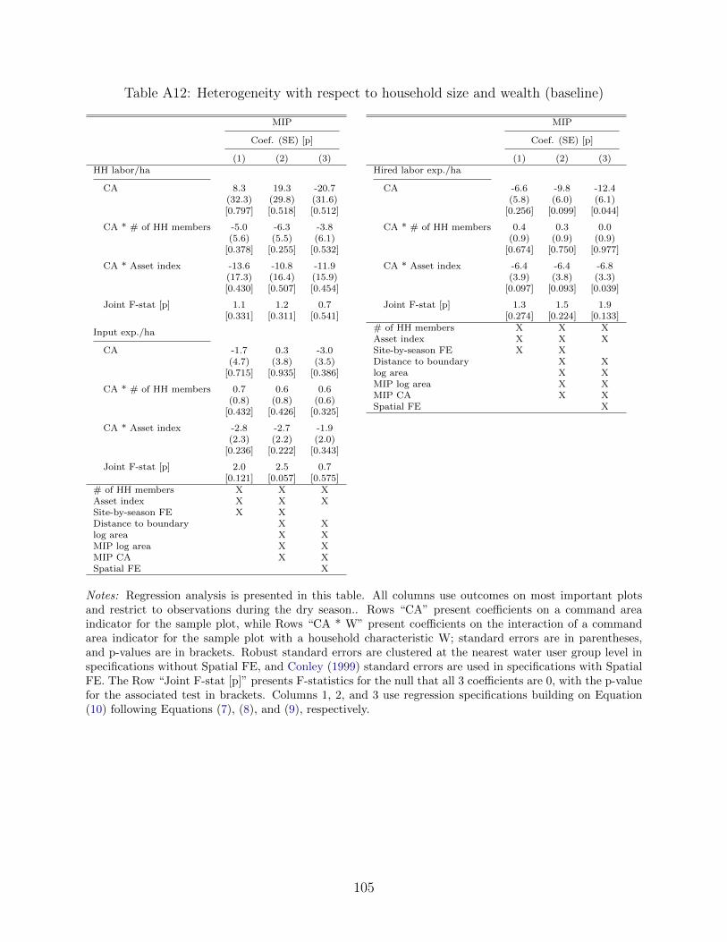
Table A12: Heterogeneity with respect to household size and wealth (baseline)

MIP

Coef. (SE) [p]

(1) (2) (3)HH labor/ha

CA 8.3 19.3 -20.7(32.3) (29.8) (31.6)[0.797] [0.518] [0.512]

CA * # of HH members -5.0 -6.3 -3.8(5.6) (5.5) (6.1)

[0.378] [0.255] [0.532]

CA * Asset index -13.6 -10.8 -11.9(17.3) (16.4) (15.9)[0.430] [0.507] [0.454]

Joint F-stat [p] 1.1 1.2 0.7[0.331] [0.311] [0.541]

Input exp./ha

CA -1.7 0.3 -3.0(4.7) (3.8) (3.5)

[0.715] [0.935] [0.386]

CA * # of HH members 0.7 0.6 0.6(0.8) (0.8) (0.6)

[0.432] [0.426] [0.325]

CA * Asset index -2.8 -2.7 -1.9(2.3) (2.2) (2.0)

[0.236] [0.222] [0.343]

Joint F-stat [p] 2.0 2.5 0.7[0.121] [0.057] [0.575]

# of HH members X X XAsset index X X XSite-by-season FE X XDistance to boundary X Xlog area X XMIP log area X XMIP CA X XSpatial FE X

MIP

Coef. (SE) [p]

(1) (2) (3)Hired labor exp./ha

CA -6.6 -9.8 -12.4(5.8) (6.0) (6.1)

[0.256] [0.099] [0.044]

CA * # of HH members 0.4 0.3 0.0(0.9) (0.9) (0.9)

[0.674] [0.750] [0.977]

CA * Asset index -6.4 -6.4 -6.8(3.9) (3.8) (3.3)

[0.097] [0.093] [0.039]

Joint F-stat [p] 1.3 1.5 1.9[0.274] [0.224] [0.133]

# of HH members X X XAsset index X X XSite-by-season FE X XDistance to boundary X Xlog area X XMIP log area X XMIP CA X XSpatial FE X

Notes: Regression analysis is presented in this table. All columns use outcomes on most important plotsand restrict to observations during the dry season.. Rows “CA” present coefficients on a command areaindicator for the sample plot, while Rows “CA * W” present coefficients on the interaction of a commandarea indicator for the sample plot with a household characteristic W; standard errors are in parentheses,and p-values are in brackets. Robust standard errors are clustered at the nearest water user group level inspecifications without Spatial FE, and Conley (1999) standard errors are used in specifications with SpatialFE. The Row “Joint F-stat [p]” presents F-statistics for the null that all 3 coefficients are 0, with the p-valuefor the associated test in brackets. Columns 1, 2, and 3 use regression specifications building on Equation(10) following Equations (7), (8), and (9), respectively.

105

Table A13: Sample plots

Dry season Rainy seasons

Dep. var. Coef. (SE) [p] Dep. var. Coef. (SE) [p]

(1) (2) (3) (4) (5) (6) (7) (8)Tracked 0.032 0.018 0.023 0.035 0.047 0.011 0.019 0.036

(0.177) (0.010) (0.014) (0.019) (0.211) (0.011) (0.016) (0.023)2,907 [0.056] [0.083] [0.069] 4,845 [0.306] [0.224] [0.114]

Missing 0.060 0.111 0.127 0.103 0.064 0.102 0.121 0.094(0.238) (0.020) (0.025) (0.028) (0.244) (0.020) (0.026) (0.028)2,907 [0.000] [0.000] [0.000] 4,845 [0.000] [0.000] [0.001]

Reason data is missing

HH attrition 0.038 0.007 0.032 0.034 0.039 0.007 0.032 0.035(0.192) (0.014) (0.019) (0.022) (0.194) (0.014) (0.019) (0.022)2,907 [0.590] [0.096] [0.129] 4,845 [0.601] [0.096] [0.121]

Rented out comm. farmer 0.012 0.102 0.092 0.069 0.011 0.099 0.089 0.064(0.108) (0.017) (0.019) (0.015) (0.105) (0.016) (0.019) (0.015)2,907 [0.000] [0.000] [0.000] 4,845 [0.000] [0.000] [0.000]

Transaction (not tracked) 0.010 0.002 0.003 0.001 0.014 -0.004 0.000 -0.005(0.099) (0.005) (0.005) (0.007) (0.116) (0.005) (0.006) (0.008)2,907 [0.681] [0.539] [0.921] 4,845 [0.465] [0.945] [0.542]

Site-by-season FE X X X XDistance to boundary X X X Xlog area X X X XSpatial FE X X

Notes: Regression analysis is presented in this table. Columns 1 through 4 restrict to observations duringthe dry season, while columns 5 through 8 restrict to observations during the rainy season. Columns 1and 5 present, for sample plots in the main discontinuity sample that are outside the command area, themean of the dependent variable, the standard deviation of the dependent variable in parentheses, and thetotal number of observations. Columns 2 through 4 and 6 through 8 present regression coefficients on acommand area indicator, with standard errors in parentheses, and p-values in brackets. Robust standarderrors are clustered at the nearest water user group level in specifications without Spatial FE, and Conley(1999) standard errors are used in specifications with Spatial FE. Columns 2 and 6 use the specification inEquation (1). Columns 3 and 7 use the regression discontinuity specification in Equation (2). Columns 4and 8 use the spatial fixed effects specification in Equation (3).

106