facilitating savings for agriculture: field experimental ... · february 2015 previously titled ......
TRANSCRIPT

NBER WORKING PAPER SERIES
FACILITATING SAVINGS FOR AGRICULTURE:FIELD EXPERIMENTAL EVIDENCE FROM MALAWI
Lasse BruneXavier Giné
Jessica GoldbergDean Yang
Working Paper 20946http://www.nber.org/papers/w20946
NATIONAL BUREAU OF ECONOMIC RESEARCH1050 Massachusetts Avenue
Cambridge, MA 02138February 2015
Previously titled “Commitments to Save: A Field Experiment in Rural Malawi.” We thank Niall Keleher,Lutamyo Mwamlima and the IPA staff in Malawi; Steve Mgwadira, Mathews Kapelemera, and WebsterMbekeani of OBM; and the OBM management and staff of Kasungu, Mponela and Lilongwe branches.Matt Basilico and Britni Must provided excellent research assistance. We are grateful to Beatriz Armendariz,Orazio Attanasio, Oriana Bandiera, Abhijit Banerjee, Luc Behagel, Marcel Fafchamps, MaitreeshGhatak, Marc Gurgand, Sylvie Lambert, Kim Lehrer, Rocco Macchiavello, Lou Maccini, Sharon Maccini,Marco Manacorda, Costas Meghir, Rohini Pande, Albert Park, Imran Rasul, Chris Woodruff, BilalZia, Andrew Zeitlin, and seminar participants at the FAI Microfinance Innovation Conference, OhioState, London School of Economics, Warwick, Institute for Fiscal Studies, Paris School of Economics,and Oxford for helpful comments. We appreciate the support of David Rohrbach (World Bank) andJake Kendall (Bill & Melinda Gates Foundation). We are grateful for research funding from the WorldBank Research Committee and the Bill & Melinda Gates Foundation. The views expressed in thispaper are those of the authors and should not be attributed to the World Bank, its executive directors,or the countries they represent. The views expressed herein are those of the authors and do not necessarilyreflect the views of the National Bureau of Economic Research.
NBER working papers are circulated for discussion and comment purposes. They have not been peer-reviewed or been subject to the review by the NBER Board of Directors that accompanies officialNBER publications.
© 2015 by Lasse Brune, Xavier Giné, Jessica Goldberg, and Dean Yang. All rights reserved. Shortsections of text, not to exceed two paragraphs, may be quoted without explicit permission providedthat full credit, including © notice, is given to the source.

Facilitating Savings for Agriculture: Field Experimental Evidence from MalawiLasse Brune, Xavier Giné, Jessica Goldberg, and Dean YangNBER Working Paper No. 20946February 2015JEL No. D03,D91,O16,Q14
ABSTRACT
We implemented a randomized intervention among Malawian farmers aimed at facilitating formalsavings for agricultural inputs. Treated farmers were offered the opportunity to have their cash cropharvest proceeds deposited directly into new bank accounts in their own names, while farmers in thecontrol group were paid harvest proceeds in cash (the status quo). The treatment led to higher savingsin the months immediately prior to the next agricultural planting season, and raised agricultural inputusage in that season. We also find positive treatment effects on subsequent crop sale proceeds andhousehold expenditures. Because the treatment effect on savings was only a small fraction of the treatmenteffect on the value of agricultural inputs, mechanisms other than alleviation of savings constraintsper se are needed to explain the treatment’s impact on input utilization. We discuss other possiblemechanisms through which treatment effects may have operated.
Lasse BruneYale UniversityEconomic Growth Center27 Hillhouse AveNew Haven, CT [email protected]
Xavier GinéThe World Bank1818 H Street N.W.Mail Stop MC 3-307Washington, D.C. [email protected]
Jessica GoldbergUniversity of MarylandDepartment of Economics3115G Tydings HallCollege Park, MD [email protected]
Dean YangUniversity of MichiganDepartment of Economics andGerald R. Ford School of Public Policy735 S. State Street, Room 3316Ann Arbor, MI 48109and [email protected]
1
1. Introduction
Agriculture in Sub-Saharan Africa employs two-thirds of the labor force and
generates about one-third of GDP growth. According to the 2008 World Development
Report, GDP growth originating in agriculture is about four times more effective in
reducing poverty than GDP growth originating outside agriculture. For this reason,
policies that foster agricultural productivity can have a substantial impact on food
security and poverty reduction.
In recent decades, there has been substantial interest among policy-makers,
donors, and international development institutions in microfinance (financial services for
the poor) as an anti-poverty intervention. Provision of microcredit has perhaps attracted
the most attention. In 2009, the Microcredit Summit estimated that there were more than
3,500 microfinance institutions around the world with 150 million clients (Daley-Harris
2009). While these outreach numbers are impressive, microcredit today is largely devoted
to non-agricultural activities (Morduch 1999; Armendariz de Aghion and Morduch 2005)
due to the substantial challenges inherent in agricultural lending.1 Given the limited
supply of credit for agriculture, many donors and academics (for example, Deaton 1990;
Robinson 2001 and more recently the Bill and Melinda Gates Foundation) have
emphasized the potential for increasing access to formal savings.2
The motivating question of this study is whether facilitating formal savings can
promote agricultural development. To this end, we collaborated with a bank and private
sector firms to implement a randomized controlled trial of a program facilitating formal
savings for Malawian cash crop (tobacco) farmers. To our knowledge, this is the first
randomized study of the agricultural impacts of an intervention facilitating savings in a
formal banking institution.
1 Giné, Goldberg, and Yang (2012) find that imperfect personal identification leads to asymmetric information problems (both adverse selection and moral hazard) in the rural Malawian credit market. 2 Aportela (1999) finds that a post-office savings expansion in Mexico raised savings by 3-5 percentage points. Burgess and Pande (2005) find that a policy-driven expansion of rural banking reduced poverty in India, and provide suggestive evidence that deposit mobilization and credit access were intermediating channels. Bruhn and Love (2009) find that bank branch openings by consumer durable stores in Mexico leads to increases in the number of informal business owners, in total employment, and in average income.

2
In advance of the May-July 2009 harvest season, farmers were randomized into a
control group or one of several treatment groups. Formal savings were facilitated for
farmers in the treatment group by offering them the opportunity to have their cash-crop
proceeds from the upcoming harvest channeled into bank accounts that would be opened
for them, in their own names. Two main variants of this treatment were implemented: 1)
an “ordinary” savings treatment, where the bank accounts offered had no special features,
and 2) a “commitment” savings treatment, in which farmers had the option of saving in
special accounts that disallowed withdrawals until a set date (chosen by the account
owner). In addition, these treatments were cross-randomized with another treatment
intended to create variation in the public observability of savings balances (details are
explained in Section 2).
Treated farmers were encouraged to use these accounts to save for future
agricultural input purchases. Farmers in the control group, on the other hand, also
received the generic encouragement to save for future agricultural input purchases, but
did not receive any facilitation of formal savings accounts, and were simply paid their
crop sale proceeds in cash (which was the status quo). We examine treatment impacts on
savings at the partner bank (observed in administrative data) as well as on agricultural
and other household outcomes (via a household survey).
The first key finding is that there are positive and statistically significant
treatment effects on a range of outcomes. Facilitating formal savings leads to higher
deposits into formal savings accounts at the partner bank, higher savings at the partner
bank immediately prior to the next planting season (November-December 2009), higher
agricultural input expenditures in that season, higher output in the subsequent harvest
(May-July 2010), and higher per capita consumption in the household after that harvest.
Impacts on agricultural input expenditures and on output are substantial, amounting to
increases over the control group mean of 13.3% and 21.4% respectively.
The second key finding is somewhat unexpected, and has to do with the
mechanism through which treatment translates into agricultural outcomes. Ex ante, the
leading candidate mechanism was the alleviation of savings constraints. In the status quo,
farmers have imperfect means of preserving funds between harvest and the subsequent
3
planting season. Depletion of funds not held in bank accounts over this period could be
due to self-control problems, demands for sharing with one’s social network, and losses
due to other factors (e.g., theft, fire). Improving access to formal savings would therefore
give farmers a better means of preserving funds between harvest and the subsequent
planting, leading to increases in agricultural input expenditures (and then to
improvements on other subsequent related outcomes).
Our results indicate, however, that only a fraction of the treatment effect on
agricultural input expenditures is likely to be attributable to alleviating formal savings
constraints. While amounts initially deposited into the accounts would have been
sufficient to pay for the increase in agricultural input expenditures that we observe,
administrative data from the bank reveals that the majority of these funds were
withdrawn almost immediately after being deposited. Three months later, just prior to the
end-of-2009 planting season treated farmers still had 1,863 Malawi kwacha (USD 12.85)
higher savings than did control-group farmers, but the treatment effect on agricultural
input expenditures is higher by a factor of four: MK 8,023 (USD 55.33).3 Therefore, only
about a quarter of the effect of the treatment on agricultural input expenditures can be
attributed to alleviation of savings constraints per se.4
We discuss a variety of mechanisms for which we are able to provide incomplete
evidence as well other mechanisms that can be ruled out. In the end, with the design
implemented and data available we are not able to identify the precise mechanisms
through which our treatment effects operated. For example, the funds held in accounts
may have served as a buffer stock, allowing farmers to self-insure and take on more risk
(by investing more in agricultural inputs). Alternately, the existence of the accounts could
have helped study participants resist demands to share resources with their social
network. Behavioral phenomena such as mental accounting or reference-dependence also
provide possible explanations. We must leave exploration of these and other possible
mechanisms to future work.
3 The exchange rate at the time of the study was MK145/USD.
4The low balances in the accounts results in low power to detect effects of the raffle treatments. Therefore, while in total there were six different randomly-assigned treatment types, differences in impacts across treatments are typically not statistically significantly different from one another, so we place little emphasis on differentiating impacts across treatment types in this paper.

4
This paper contributes to the burgeoning literature on the effects of formal savings
accounts, and in particular of making offers of commitment savings. Dupas and Robinson
(2013a) offer ordinary savings accounts to Kenyan urban entrepreneurs, finding positive
impacts on investment and income for women. In this paper, by contrast, we test the
effect of direct deposit of agricultural proceeds into ordinary and commitment savings
accounts. Prina (2014) finds that random assignment of basic savings account access to
households in Nepal leads to increases in financial assets and in human capital
investments. Atkinson et al. (2010) offer microcredit borrowers in Guatemala savings
accounts with different features, including reminders about a monthly commitment to
save and a default of 10% of loan repayment as a suggested monthly savings target. They
find that both features increase savings balances substantially. Dupas and Robinson
(2013b) test the impact of commitment features for health savings in western Kenyan
ROSCAs; their qualitative findings from a post-intervention survey are suggestive of a
mental accounting channel.
The remainder of this paper is organized as follows. The next section describes
the experimental design and data sources. Section 3 describes our empirical specification.
Section 4 presents the treatment effect estimates. Section 5 then considers evidence on
the mechanisms through which the treatment effects may have operated. Section 6
concludes.
2. Experimental design and survey data
The experiment was a collaborative effort between Opportunity Bank of Malawi
(OBM),5 Alliance One, Limbe Leaf, the University of Michigan and the World Bank.
Opportunity International is a private microfinance institution operating in 24 countries
that offers savings and credit products; in Malawi, it has a full banking license that allows
it to collect deposits and on-lend funds. Alliance One and Limbe Leaf are two large
private agri-business companies that offer extension services and high-quality inputs to
5 At the time of the study, our bank partner went by the company name Opportunity International Bank of Malawi (OIBM), but has since changed its name to Opportunity Bank of Malawi (OBM).

5
smallholder farmers via an out-grower tobacco scheme.6 These two companies work with
smallholder out-growers by organizing them geographically into clubs of 10-20 members
who obtain tobacco production loans under group liability from OBM.7 Tobacco clubs
meet regularly and sell their crop output collectively to the tobacco auction floor. In the
central Malawi region we study, tobacco farmers have similar poverty and income levels
to those of non-tobacco-producing households.8
While all farmers in the study were loan customers of OBM at the start of the
project, the loans provided a fixed input package that for the majority of farmers fell short
of optimal levels of fertilizer use on their tobacco plots.9 This is important because it
suggests that there is room for savings to increase input utilization. In addition, while a
minority of farmers was using optimal levels of fertilizer for the amount of land they
were cultivating at baseline, even those farmers could use savings generated by the
intervention to obtain additional inputs and expand land under tobacco cultivation, or
shift land devoted to other crops towards tobacco. Finally, the savings intervention could
also affect use of fertilizer and other inputs on maize (the main staple crop in Malawi)
and other crops.10
6 Tobacco is central to the Malawian economy, as it is the country’s main cash crop. About 70% of the country’s foreign exchange earnings come from tobacco sales, and a large share of the labor force works in tobacco and related industries. 7 The cost of an input loan includes an interest rate of 28% percent per year and a one-time 2.5% processing fee. 8 Based on authors’ calculations from the 2004 Malawi Integrated Household Survey (IHS), individuals in tobacco farming rural households in central Malawi live on PPP$1.46/day on average, while the corresponding average for non-tobacco farmers is PPP$1.51/day. That said, the two groups are different in other ways. Tobacco farmers have somewhat larger households (6.68 persons compared to 4.94 persons for households not farming tobacco), higher levels of education of the household head (5.61 years compared to 4.63 years) and a higher share of school age kids (6-17 years) currently in school conditional on having school age children (88.1% compared to 77.9%). 9 The input package was designed for a smaller cultivated area. As a result, 60.4% of farmers were applying less than the recommended amount of nitrogen on their tobacco plots at baseline. The figures for the two other key nutrients for tobacco are even more striking: 83.2% and 84.7% of farmers used less than the recommended amount of phosphorus and potassium, respectively. For each of the three nutrients, among farmers using less than recommended levels, the mean ratio of actual use to optimal use was about 0.7. Optimal use levels were determined by Alliance One and Limbe Leaf in collaboration with Malawi’s Agricultural Research and Extension Trust (ARET), and are similar to nutrient level recommendations in the United States (Pearce et al. 2011). 10 At baseline, 89.5% and 99.9% of farmers were applying less than the recommended amount of nitrogen and phosphorus, respectively, on their maize plots and 44.1% and 98.6% of farmers applied less than half the recommended amounts for the two nutriens. Among farmers applying less than the recommended amount of nitrogen (phosphorus) on maize, the ratio of actual use to optimal use was 0.48 (0.14). Potassium

6
The experiment was designed to test the impact of facilitating savings in formal
bank accounts. In addition, we sought to test whether offering accounts with
“commitment” features would have a greater impact than offering “ordinary” bank
accounts without such features.11 Farmer clubs were randomly assigned to either a
control group offered no savings facilitation, an “ordinary savings” treatment group that
was offered assistance setting up direct deposit into individual, liquid savings accounts,
and a “commitment savings” treatment group that was offered assistance setting up direct
deposit into individual ordinary savings accounts and additional accounts with
commitment features.
The design of the experiment also aimed to explore the role of savings accounts in
helping farmers resist pressure to share resources with others in their social network.
Farmer clubs in the ordinary and commitment savings treatment groups were further
cross-randomized into sub-groups that were or were not entered into a raffle wherein they
could win prizes based on their account balances (described further below).
In sum, the two cross-cutting interventions result in seven treatment conditions: a
pure control condition without savings account offers or raffles; ordinary savings
accounts with no raffles, with private distribution of raffle tickets, and with public
distribution of raffle tickets; and commitment savings accounts with no raffles, with
private distribution of raffle tickets, and with public distribution of raffle tickets (see
Table 2).
Figure 1 presents the timing of the experiment with reference to the Malawian
agricultural season. The baseline survey and interventions were administered in April and
May 2009, immediately before the 2009 harvest. As a result, farmers in the commitment
treatment group made allocation decisions into the commitment and ordinary accounts in is not recommended for maize cultivated in central Malawi. Nutrient recommendations are from Benson (1999). 11 Research on savings accounts with features that self-aware individuals can use to limit their options in anticipation of future self-control problems includes Ashraf, Karlan, and Yin (2006), who investigate demand for and impacts of a commitment savings device in the Philippines and find that demand for such commitment devices is concentrated among women exhibiting present-biased time preferences. Duflo, Kremer and Robinson (2011) find that offering a small, time-limited discount on fertilizer immediately after harvest has an effect on fertilizer use that is comparable to that of much larger discounts offered later, around planting time. Giné et al. (2013) find that Malawian farmers with present-biased preferences are more likely to revise a plan about how to use future income, a result that supports the potential of commitment accounts to improve welfare for those with self-control problems.

7
the “cold state” prior to receiving the net proceeds from tobacco sales.12 Planting starts
between November and December depending on the arrival of the rains. We will
therefore refer to the time from harvest until end October as the pre-planting period.
Randomization of the savings and raffle treatments was conducted at the club
level in order to minimize cross-treatment contamination.13 The sample consists of 299
clubs with 3,150 farmers surveyed at baseline (February-April 2009), for whom we can
track savings deposits, withdrawals, and balances in our partner bank’s administrative
data. In addition, we have data from an endline survey administered in July-September
2010, after the 2010 harvest, for 2,835 farmers from 298 clubs. Attrition from the
baseline to the endline survey was 10.0% and is not statistically significantly different
across different treatment groups (as shown in Online Appendix Table 1). The endline
survey will be used to examine impacts on outcomes such as farm inputs, production, and
household per capita expenditures.
Financial education
Members of all clubs attended a financial education session immediately after the
baseline survey was administered. The session reviewed basic elements of budgeting and
explained the benefits of formal savings accounts, with an emphasis on how such
accounts could be used to set aside funds for future consumption and investment. The full
script of the financial education session can be found in Appendix A.
The same financial education session was deliberately provided to all clubs –
including those subsequently assigned to the control group – so that treatment effects
could be attributed solely to the provision of the financial products, abstracting from the
effects of financial education that are implicitly provided during the product offer (for
example, strategies for improved budgeting). For this reason, we can estimate neither the
impact of the ordinary and commitment treatments without such financial education, nor
the impact of the financial education alone.
12 If decisions had been made the day that tobacco sales were transferred to OBM then the allocations into the commitment accounts by present-biased individuals would have been lower. 13 Prior to randomization, treatment clubs were stratified by location, tobacco type (burley, flue-cured or dark-fire) and week of scheduled interview. The stratification of treatment assignment resulted in 19 distinct location/tobacco-type/week stratification cells.

8
Savings treatments
Implementation of the savings treatments took advantage of the existing system of
depositing crop sale proceeds into OBM bank accounts. At harvest, farmers sold their
tobacco to the company at the price prevailing on the nearest tobacco auction floor.14 For
farmers in the control group, the proceeds from the sale were then electronically
transferred to OBM, which deducted the loan repayment (plus fees and surcharges) of all
borrowers in the club, and then credited the remaining balance to a club account at OBM.
Club members authorized to access the club account (usually the chairman or the
treasurer) came to OBM branches and withdrew the funds in cash.
Farmers in the ordinary savings treatment were offered account opening
assistance and the opportunity to have their harvest proceeds (net of loan repayment)
directly deposited into individual accounts in their own individual names (see Figure 2
for a schematic illustration of the money flows). These ordinary savings accounts are
regular OBM savings accounts with an annual interest rate of 2.5%. After their crop was
sold, farmers traveled to the closest OBM branch to confirm that funds were available at
the club level, i.e. that club proceeds exceeded the club’s loan obligation. Authorized
members of the clubs (often accompanied by other club members) then filled out a sheet
specifying the division of the balance of the club account between farmers. Funds were
transferred into the individual accounts of club members who had opted to open them.
Other club members received their share of the money in cash.
Farmers in clubs assigned to the ordinary savings treatment were offered only one
(ordinary) savings account. Farmers assigned to the commitment treatment had the
option of opening an additional account with commitment features. The commitment
savings account had the same interest rate as the ordinary account, but allowed farmers to
specify an amount to be transferred to this illiquid account, and a “release date” when the
bank would allow access to the funds.15 During the account opening process, farmers
14 The tobacco growing regions are divided among the two tobacco buyer companies. In their coverage area each buyer company organizes farmers into clubs and provides them with basic extension services. 15 By design, funds in the commitment account could not be accessed before the release date. In a small number of cases OBM staff allowed early withdrawals of funds when clients presented evidence of emergency needs, e.g. health or funeral expenditures.

9
stated how much they wanted deposited in the ordinary and commitment savings
accounts after the sale of their tobacco crops. For example, if a farmer stated that that he
wanted MK 40,000 in an ordinary account and MK 25,000 in a commitment savings
account, funds would first be deposited into the ordinary account until MK 40,000 had
been deposited, then into the commitment savings account for up to MK 25,000, with any
remainder being deposited back into the ordinary account. The choice of a “trigger
amount” that had to flow into the ordinary account before any money would be deposited
into the commitment account turns out to be important, because many farmers chose
triggers higher than their eventual crop sale revenue, and therefore ended up without
deposits into their commitment accounts. Opening the commitment account or ordinary
account only was not an option, although farmers could have set the “trigger amount” to
zero or a very large amount if they only wanted to use the ordinary or commitment
account, respectively. No fees were charged for the initial post-crop-sale deposits into
the ordinary or commitment accounts. Further details on account features and fees can be
found in Appendix A.
Farmers who were not offered a particular account type due to their treatment
status (e.g., control group farmers who were not offered either type of account, or
ordinary treatment group farmers who were not offered the commitment account) but
learned about and requested them were not denied those accounts, but they were not
given information about or assistance in opening them.16 In other words, the savings
treatments were implemented as an encouragement design.
Raffle Treatments
To study the impact of public information on savings and investment behavior,
we implemented a cross-cutting randomization of a savings-linked raffle. Participants in
each of the two savings treatments were randomly assigned to one of three raffle
16 During the baseline interaction with study participants, no farmers in the control group expressed to our survey staff a desire for either ordinary or commitment accounts, and none in the ordinary treatment group requested commitment accounts. According to OBM administrative records, seven individuals in the control group (1.7%) and 52 farmers in the ordinary treatment group (3.7%) had commitment accounts by the end of October 2009 (these were opened without our assistance or encouragement). None of these farmers had any transactions in the accounts.
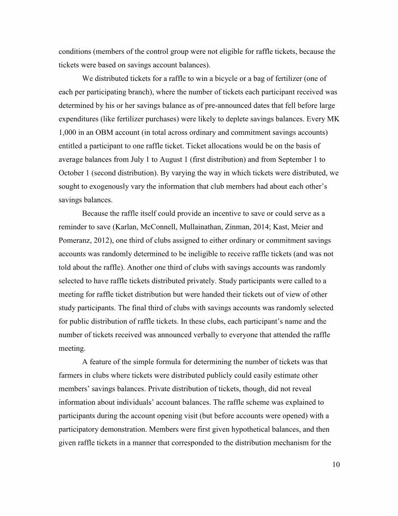
10
conditions (members of the control group were not eligible for raffle tickets, because the
tickets were based on savings account balances).
We distributed tickets for a raffle to win a bicycle or a bag of fertilizer (one of
each per participating branch), where the number of tickets each participant received was
determined by his or her savings balance as of pre-announced dates that fell before large
expenditures (like fertilizer purchases) were likely to deplete savings balances. Every MK
1,000 in an OBM account (in total across ordinary and commitment savings accounts)
entitled a participant to one raffle ticket. Ticket allocations would be on the basis of
average balances from July 1 to August 1 (first distribution) and from September 1 to
October 1 (second distribution). By varying the way in which tickets were distributed, we
sought to exogenously vary the information that club members had about each other’s
savings balances.
Because the raffle itself could provide an incentive to save or could serve as a
reminder to save (Karlan, McConnell, Mullainathan, Zinman, 2014; Kast, Meier and
Pomeranz, 2012), one third of clubs assigned to either ordinary or commitment savings
accounts was randomly determined to be ineligible to receive raffle tickets (and was not
told about the raffle). Another one third of clubs with savings accounts was randomly
selected to have raffle tickets distributed privately. Study participants were called to a
meeting for raffle ticket distribution but were handed their tickets out of view of other
study participants. The final third of clubs with savings accounts was randomly selected
for public distribution of raffle tickets. In these clubs, each participant’s name and the
number of tickets received was announced verbally to everyone that attended the raffle
meeting.
A feature of the simple formula for determining the number of tickets was that
farmers in clubs where tickets were distributed publicly could easily estimate other
members’ savings balances. Private distribution of tickets, though, did not reveal
information about individuals’ account balances. The raffle scheme was explained to
participants during the account opening visit (but before accounts were opened) with a
participatory demonstration. Members were first given hypothetical balances, and then
given raffle tickets in a manner that corresponded to the distribution mechanism for the
11
treatment condition to which the club was assigned. In clubs assigned to private
distribution, members were called up one by one and given tickets in private (out of sight
of other club members). In clubs assigned to public distribution, members were called up
and their number of tickets was announced to the group. Since real tickets based on
actual account balances were distributed twice during the experiment, the first
distribution also functioned as an additional demonstration. As reported in Section 4
below, however, substantial withdrawals from both the ordinary and commitment
accounts occurred soon after funds were deposited, and as a result, this public revelation
treatment was likely to have had little effect.
Sample
Table 1 presents summary statistics of baseline household and farmer club
characteristics. All variables expressed in money terms are in Malawi Kwacha
(MK145/USD during the study period). Baseline survey respondents own an average of
4.7 acres of land and are mostly male (only six percent were female). Respondents are on
average 45 years old. They have an average of 5.5 years of formal education, and have
low levels of financial literacy.17 Sixty three percent of farmers at baseline had an
account with a formal bank (mostly with OBM).18 The average reported savings balance
in bank accounts at the time of the baseline was MK 2,083 (USD 14), with an additional
MK 1,244 (USD 9) saved in the form of cash at home.
Balance of baseline characteristics across treatment conditions
To examine whether randomization across treatments achieved balance in pre-
treatment characteristics, Table 3 presents the differences in means of 17 baseline
variables in the same format as used for the subsequent analysis. Panel A checks for
balance between the control group and the treatment group, the latter pooled across all of
17 In particular, 42% of respondents were able to compute 10% of 10,000, 63% were able to divide MK 20,000 by five and only 27% could apply a yearly interest rate of 10% to an initial balance to compute the total savings balance after a year. 18 This number includes a number of “payroll” accounts opened in a previous season by OBM and one of the tobacco buyer companies as a payment system for crop proceeds, and which do not actually allow for savings accumulation. Our baseline survey unfortunately did not properly distinguish between these two types of accounts.

12
the savings and raffle treatments. Panel B looks for differences between the control
group, the ordinary savings group, and the commitment savings group, with each of the
savings treatments pooled across their respective raffle sub-treatments.
With a few exceptions, the sample is well balanced. We test balance for 17
baseline variables. In Panel A, respondents assigned to the savings treatment are four
percentage points more likely to be female and two percentage points less likely to be
married than those assigned to the control group. At baseline, they report spending
nearly MK 4,000 more in cash on agricultural inputs, a difference that is statistically
significant at the 90 percent confidence level.
Panel B reveals that respondents in both the commitment and ordinary treatment
groups are more likely to be female and less likely to be married. The treatment-related
imbalance with respect to cash spent on inputs found in Panel A appears to be driven by
imbalance in the ordinary treatment group, which is different from the control group at
the 5% level (the difference between the commitment treatment group and the control
group for that variable is not statistically significant at conventional levels). This pattern
of imbalance contrasts with the pattern of treatment effects (in results below), in which
statistically significant effects (and larger point estimates) are concentrated in the
commitment treatment (rather than the ordinary treatment), and therefore may assuage
concerns that the baseline imbalance is driving the estimated treatment effects. Those in
the commitment treatment group are also less likely to be patient now and impatient later,
compared to the control group (significant at the 5% level).
The baseline characteristics in Table 3, plus stratification cell fixed effects, are
included as controls in the main regressions. This concords with the recommendations in
Bruhn and McKenzie (2009) to include stratification cell fixed effects in stratified
randomization designs, and also to control for baseline variables that are highly
correlated with the post-treatment outcomes of interest (which, in our case, include
baseline savings and key agricultural decisions such as land and input utilization).
3. Empirical specification

13
We study the effects of our experimental interventions on several sets of
outcomes: deposits into and withdrawals from savings accounts, savings balances,
agricultural outcomes from the next year’s growing season and household expenditure
following that season, households’ financial interactions with others in their network, and
future use of financial products. These data come from the endline survey administered
after the 2010 harvest, and from administrative data on bank transactions and account
balances collected throughout the project.
We present two regression specifications reported as separate panels in the main
results tables. The first tests the effect of being randomly assigned to any of the savings
facilitation treatments, relative to being assigned to the control group. In Panel A of the
subsequent tables, we run regressions of the form
Yij= δ + αSavingsj + β’Xij + εij (1)
Yij is the dependent variable of interest for farmer i in club j. Savingsj is an indicator
variable for club-level assignment to either of the two savings treatment groups. The
coefficient α measures the effect of being offered direct deposit into an individual savings
account (either ordinary savings accounts only or ordinary plus commitment accounts).
Xij is a vector that includes stratification cell dummies and the 17 household
characteristics measured in the baseline survey prior to treatment, and summarized in
Table 3, and εij is a mean-zero error term. Because the unit of randomization is the club,
standard errors are clustered at this level (Moulton 1986).
In Panel B, we compare the impact of assignment to the ordinary savings
treatment to the impact of assignment to the commitment savings treatment. Regressions
are of the form
Yij= δ + γ1Ordinaryj + γ2Commitmentj + β’Xij + εij (2)
where Yij and Xij are defined as above. Ordinaryj is an indicator for club-level
assignment to the ordinary savings treatment, and Commitmentj is an indicator for
assignment to the commitment savings treatment. The coefficient γ1 represents the effect
of eligibility for direct deposit into ordinary accounts only, relative to the control group.
γ2 captures the analogous effect for eligibility for direct deposit into ordinary accounts
and automatic transfers into commitment savings accounts. The difference between
14
those two coefficients, then, captures the marginal effect of the commitment savings
account relative to direct deposit into the ordinary account. The p-value for the test of the
null hypothesis that γ1 = γ2 is reported at the bottom of each Panel B.
Both regression equations (1) and (2) measure treatment effects that pool the
raffle sub-treatments. Results with full detail on the raffle sub-treatments (six treatments
in all) are presented in Online Appendix Tables 3-6.
Throughout the analysis, we focus on intent-to-treat (ITT) estimates because not
every club member offered account opening assistance decided to open an account. We
do not report average treatment on the treated (TOT) estimates because it is plausible that
members without accounts are influenced by the training script itself or by members who
do open accounts in the same club, either of which would violate the stable unit treatment
value assumption (SUTVA) (Angrist, Imbens and Rubin, 1996).
4. Empirical results
We first examine the effects of our experimental interventions on formal savings:
the flow of funds into and out of accounts, and savings account balances. We then turn to
the impacts on agricultural input use, farm output, household expenditures, and other
household behaviors.
Take-up and impacts on savings transactions
The first question of interest is whether the experimental treatments changed use
of individual savings accounts. Table 4 presents estimates of equations (1) and (2) (in
Panels A and B, respectively) for outcomes from administrative data on account
transactions.
Column 1 presents treatment effects on “take-up” of the offered financial
services: opening of individual bank accounts coupled with direct deposit of tobacco crop
proceeds.19 Panel A indicates that take-up was 19.4% among respondents offered any
treatment (this dependent variable is zero by design in the control group). Take-up is very 19 The time period over which this dependent variable is calculated is intentionally very broad (Mar 2009 to Apr 2010), so as to capture any direct deposit from the tobacco purchase companies into the study respondent accounts. In practice the vast majority of direct deposits took place in the May-July 2009 harvest season.
15
similar across the commitment and ordinary treatments (Panel B), and statistically
indistinguishable across them (the p-value of the difference in take-up across the two
groups is 0.432). In order to understand the drivers of take-up, Appendix Table 7 reports
the results of a probit regression of two measures of “take-up” against household and
individual characteristics. The dependent variables are a broader definition than that in
column 1 of Table 4 of opening of an account with perhaps no direct deposit (column 1)
and the more restrictive definition used in column 1 of Table 4, that is, opening of an
account and a positive direct deposit into the account (column 2). The sample in Panel A
includes all individuals in the ordinary and commitment treatment groups, while in Panel
B only individuals in the commitment group are included. The results suggest that
education, having already a formal account (perhaps opened to deposit the proceeds of a
loan) and notably net transfers (given minus received) in Panel A are all positively
correlated with both having one account opened as well as having an account opened
with a positive direct deposit. In contrast, whether the individual is hyperbolic does not
seem to predict “take-up”.
Owing to the study’s aim to promote agricultural input investments in the Nov-
Dec 2009 planting season, for the remaining dependent variables in Table 4, we examine
transactions over the months preceding that period, March through October 2009. In
column 2, the dependent variable is total deposits into all accounts at the partner bank
(these are direct deposits from the tobacco companies as well as other deposits made by
account holders). The mean of this variable in the control group is MK 3,281 (USD
21.72). Compared to this amount, the impact of being assigned to any treatment group
shown in Panel A is large (MK 17,609, or USD 121.44) and statistically significantly
different from zero at the 1% level. Given that take-up was very similar across the two
treatment groups, and that take-up by design meant that all crop proceeds were deposited
with the partner bank, it should not be surprising that the treatment effect is very similar
across commitment and ordinary treatment groups (Panel B). Each separate treatment
effect is statistically significantly different from zero at the 1% level, but the treatment
effects are not statistically significantly different from one another (p-value 0.642).
16
The next three columns provide more detail on the types of account into which
deposits were destined, examining treatment effects on deposits into ordinary accounts,
commitment accounts, and “other” accounts that study participants might have held at the
partner bank (which we did not assist in opening). The vast majority of deposits were into
ordinary savings accounts. Treatment effects on that outcome (Panels A and B of column
3) are very similar in magnitude and statistical significance levels to those for total
deposits in column 2.
In contrast, treatment effects on deposits into commitment accounts were much
smaller (column 4). Panel A reveals that respondents assigned to any treatment group
deposited less than MK 700 into a commitment account (significant at the 1% level), but
that figure pools across individuals offered the commitment savings accounts and those
offered ordinary accounts only. In Panel B, as we might expect, the impact of the
ordinary treatment is very close to zero (and not statistically significant), while the impact
of the commitment treatment is MK 1,490 (USD 10.28) and statistically significant at the
1% level. Results in column 4 reveal that the encouragement design had the intended
effect of increasing use of illiquid savings instruments in the commitment treatment
group. While impacts on commitment savings balances are positive and statistically
significant, it is clear commitment savings deposits are substantially lower than deposits
into ordinary accounts, even among those offered the commitment treatment.
Column 5 indicates that there were no large or statistically significant treatment
effects on deposits into other partner bank accounts that were not offered by the project.
Treatment effects on withdrawals in the pre-planting period (column 6) are nearly
as large in magnitude as effects on deposits. The “any treatment” coefficient in Panel A
as well as the separate commitment and ordinary treatment coefficients in Panel B are all
statistically significantly different from zero at the 1% level.
Time patterns of deposits and withdrawals
A key aim of this project was to promote savings for agricultural input
investments, by facilitating individual bank account opening and channeling substantial
resources (respondents’ own crop proceeds) into those accounts. The results in Table 4
17
are therefore sobering, in that both deposits into and withdrawals from OBM accounts in
the 2009 pre-planting period were substantial for both the commitment and ordinary
treatments.
A question of interest is whether funds remained deposited in the accounts until
the following planting period (November-December 2009), when agricultural inputs are
typically applied. As it turns out, in many cases funds in ordinary accounts were
withdrawn relatively quickly after the initial deposit of crop proceeds was made. About
22 percent of the initial deposits into ordinary accounts were followed by withdrawals on
the same day of nearly equal amounts.20 On average, only 26 percent of the original
balance remained in an ordinary savings account two weeks after it was initially
deposited.
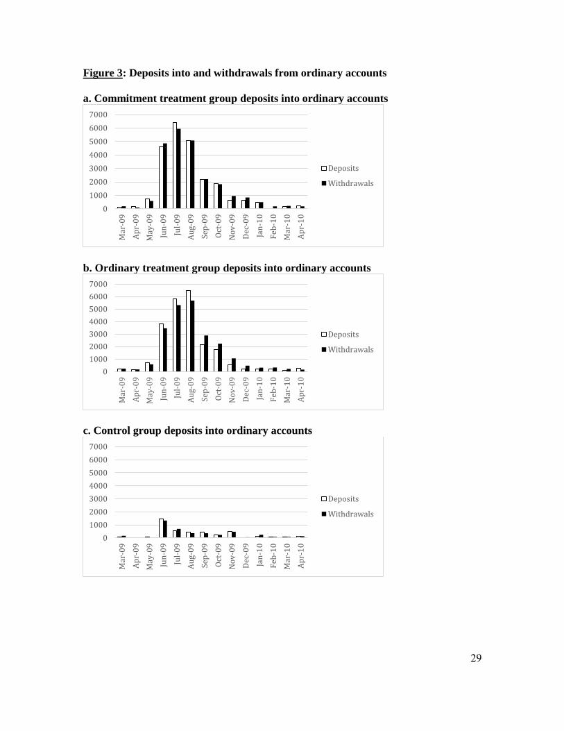
Figure 3 presents average deposits into and withdrawals from ordinary and other
(non-commitment) accounts, by month, from March 2009 to April 2010.21 The sample in
Figure 3.a is individuals in the commitment treatment, while the sample for Figure 3.b is
individuals in the ordinary treatment. For comparison, the sample used in Figure 3.c is
individuals in the control group.
The figures indicate that peak deposits occurred in June, July, and August 2009,
coinciding with the peak tobacco sales months. Average deposits in every month for
individuals in both the commitment and ordinary treatments are quite similar in
magnitude to average withdrawals, indicating that the majority of deposited funds were
withdrawn soon thereafter. As a result, savings balances during the pre-planting period
were much lower than deposited amounts, explaining why most farmers did not
participate in the raffle.22
One likely reason funds in the ordinary accounts were withdrawn soon after they
had been deposited has to do with transaction costs. Farmers lived on average 20
kilometers away from the bank branch and would typically travel there by foot, bus, or
bicycle.23 In addition to travel time, farmers report a median waiting time at the branch to
20 See Appendix B for details about the construction of deposit spells underlying these calculations. 21 The data presented are the sum of the dependent variables in columns 4 and 6 of Table 4. 22 The pattern is similar for individuals in the control group, but levels are much lower owing to the fact that direct deposit from the tobacco auction floor into farmer accounts was not enabled for that group. 23 The median round-trip bus fare is MK 400 and takes two hours each way.

18
withdraw money of one hour.
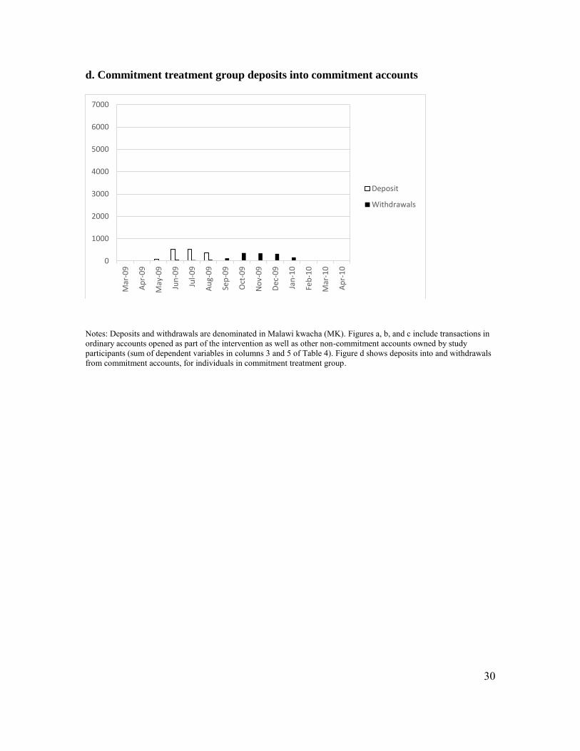
In contrast to the time pattern of the ordinary accounts, funds into commitment
accounts do stay in accounts for longer periods of time. Figure 3.d displays average
deposits into and withdrawals from commitment accounts, by month, for individuals in
the commitment treatment. For deposits, the peak months are June, July, and August,
coinciding with the peak deposit months for the ordinary accounts. But withdrawals from
the commitment accounts are delayed substantially, occurring in October, November, and
December, coinciding with the key months when agricultural inputs must be purchased
and applied on fields. Of course, as revealed in Table 4, the amounts of money involved
in these transactions are much lower than those in ordinary accounts.
Impacts on savings balances
Notwithstanding the fact that substantial amounts were withdrawn from accounts
very soon after the direct deposits occurred, it is still possible that enough funds remained
in total across both types of accounts to be able to detect statistically significant effects
on savings balances. Due to our interest in facilitating savings for agricultural input
utilization in the November-December 2009 planting season, we now examine treatment
effects on savings balances immediately prior to that period.
Table 5 reports coefficient estimates from estimation of equations (1) and (2) for
savings balances in the different types of OBM accounts, on October 22, 2009. In Panel
A, which presents the impact of “any treatment,” we find that the treatment effect is
positive and statistically significantly different from zero at the 1% level for total savings
balances (column 1), ordinary savings balances (column 2), and commitment savings
balances (column 3). In addition, the coefficient in the regression for savings balances in
other accounts (column 4) is also positive and statistically significantly different from
zero at the 5% level.
In Panel B, which estimates separate effects for the commitment and ordinary
treatments, we find that the effects of each treatment on total savings balances (column 1)
are positive and statistically significantly different from zero at the 1% level. That said,
the effect of the commitment treatment is larger than that of the ordinary treatment, and

19
this difference is statistically significant at the 5% level. Effects of the treatments are very
similar on savings in ordinary accounts and on savings in other accounts (columns 2 and
4); we cannot reject equality of the ordinary and commitment treatment effects for these
outcomes at conventional significance levels. By contrast, the two treatments
(unsurprisingly) differ in their impact on savings balances in commitment savings
accounts: the commitment treatment effect is positive and statistically significantly
different from zero at the 1% level, while the ordinary treatment effect is very close to
zero and is not statistically significant. Equality of these two coefficients is rejected at the
1% level. It is therefore clear that the difference in the impacts of the commitment and
ordinary treatments on total savings (shown in column 1) is being driven by the differing
impacts on savings in commitment accounts (column 3).
These results reveal that both types of savings accounts have positive impact on
savings preservation between the May-July 2009 harvest and the November-December
2009 planting season, with the commitment treatment providing an additional boost to
savings on top of the impact of the ordinary account. The magnitudes of these effects are
not negligible, in absolute terms for rural Malawian households as well as in comparison
to control group savings of MK 364 (USD 2.36). The impact of “any treatment” on
savings from Panel A is MK 1,863 (USD 12.85). From Panel B, the impact of the
commitment savings treatment is MK 2,475 (USD 17.07) and the impact of the ordinary
treatment is MK 1,301 (USD 8.97).
Impacts on agricultural outcomes and household expenditure
In Table 6, we turn to the impacts of the treatments on agricultural outcomes in
the 2009-10 season (land cultivation, input use, crop output) and on household
expenditures after the 2010 harvest.24
Column 1 presents treatment effects on land under cultivation in acres. Panel A
indicates that land cultivated was higher by 0.30 acres among respondents offered any
treatment (statistically significant at the 5% level), compared to 4.28 acres in the control
24 All outcomes in Table 6 are for the total household, not per capita. We show in Table 7, column 1 that the treatments have no effect on household size, so interpretation of impacts in Table 6 is not clouded by concurrent changes in household size.

20
group. Treatment effects are very similar when estimated for the commitment and
ordinary treatments separately (Panel B), and the difference between the two is not
statistically significantly different from zero.25
Results in column 2, Panel A show that the treatment had a positive impact on the
total monetary value of agricultural inputs used in the 2009-10 planting season, which is
statistically significant at the 10% level. Estimating the effects separately for the
commitment and ordinary treatments reveals that both effects are positively signed, and
the effect of the commitment treatment is statistically significantly different from zero at
the 5% level. While the commitment treatment coefficient is larger in magnitude than the
ordinary treatment coefficient, we cannot reject at conventional statistical significance
levels that the two treatment coefficients are equal to one another.
The increase in agricultural input utilization caused by the treatment appears to
have, in turn, caused increases in agricultural output. Columns 3-5 show treatment effects
on, respectively, crop sale proceeds, value of crop output (both sold and unsold), and
farm profit (value of output minus value of inputs). For each of these outcomes, the “any
treatment” coefficient in Panel A is positive and statistically significant at the 5% or 10%
level. In Panel B, the commitment treatment coefficient is positive and statistically
significant in each of the regressions at the 1% or 5% level, and is larger in magnitude in
each case than the corresponding ordinary treatment coefficient. Only in column 3
(proceeds from crop sales) can we reject at conventional levels (10% in this case) the
hypothesis that the commitment and ordinary treatment coefficients are equal.26,27
Given the positive treatment effects on agricultural production, it is of interest to
examine effects on household expenditures, in column 6. The effect of any treatment is 25 We investigated whether the treatment effects on land are due to increased land rentals, and found no large or statistically significant effect (for “any treatment” and for the commitment and ordinary treatments separately). Results available from authors on request. 26 The increase in farm profit in column 5 and in the value of the inputs in column 2 suggests a high rate of return to inputs. Most of the increases in expenditures were on firewood to cure tobacco and on fertilizer. Among the different varieties of tobacco grown, the highest value one needs more curing, so the increased profits could be due to a shift in the crop mix towards higher value tobacco as well as the increased inputs. In addition, historical production and weather data suggest that 2010 was a good production year with average crop prices. 27 In results available upon request, we find that increases in production caused by the treatments are relatively concentrated in tobacco production. In the control group, tobacco accounts for 66.5% of the kwacha value of production, but increases in tobacco production account for 81.4% of the treatment effect (MK19,477 of the MK23,921 increase in the value of crop output).
21
positive and statistically significant at the 10% level (Panel A). Results in Panel B show
that both commitment and ordinary treatment effects are positive in magnitude, and the
commitment treatment effect is statistically significantly different from zero at the 5%
level. We cannot reject at conventional significance levels that the commitment and
ordinary treatment effects are equal.
The treatment effects identified in Table 6 are economically significant. In Panel
A, the treatment effect on total value of inputs is MK 8,023 (USD 55.33), amounting to
an increase of 13.3 percent over the control group mean, while the treatment effect on
value of crop (sold and unsold) is MK 23,921 (USD 164.97), an increment of 15.4
percent over the control group mean. The increase in household expenditure is 10.8
percent vis-à-vis the mean in the control group. These results show large, consistent
effects of “any treatment” on outcomes that are likely connected to household well-being.
Consistent with these findings, column 6 of Table 7 shows that being assigned to
a savings treatment group increased the probability of owning a fixed-deposit account
over a year later by 3 percentage points, a statistically significant increase of 75 percent
relative to the control group mean of 0.039.28 In addition, study participants continue to
use the offered ordinary accounts. Using the bank’s administrative data we find that
treatment effects on deposits, withdrawals, and net deposits persist during the May to
July 2010 period, more than a year after the initial intervention, particularly in the
ordinary treatment group.
The continued usage of ordinary accounts and the increased take-up of fixed
deposit accounts one year after the intervention suggest that farmers in the treatment
group found something of value in the savings products offered.
5. Mechanisms
We now turn to considering the mechanisms through which our treatment effects
may have operated. Studies of the impact of savings account access typically posit
28 In response to the positive results of this study, OBM decided to continue offering fixed deposit accounts as well as the commitment accounts (which they call “SavePlan” accounts) that were designed for the project. As of the beginning of 2015, they remain part of OBM’s deposit product offerings.

22
(implicitly or explicitly) that effects would operate via alleviation of savings constraints
(e.g., Dupas and Robinson 2013a, Prina 2014). A study population is typically thought to
have imperfect methods for preserving funds, which can be depleted for a variety of
reasons such as self-control problems, demands for sharing with one’s social network, or
theft. In our study population, alleviation of savings constraints via provision of formal
savings accounts could help farmers preserve funds between harvest and the subsequent
planting season, leading to positive impacts on agricultural input expenditures (and then
on other subsequent related outcomes).
While we do find positive treatment effects on both savings balances and on
subsequent agricultural input utilization, the relative magnitudes of the effects are
inconsistent with alleviation of savings constraints being the only mechanism at work.
Consider the impact of “any treatment” on the value of agricultural inputs used (Table 6,
column 2), MK 8,023. While the treatment did cause an increase in deposits exceeding
that amount (MK 17,609, from Table 4, column 2), withdrawals happened quite soon
after deposits, so that very little remained in the accounts some months later once the
time came for the November-December input purchases: the treatment effect on savings
balances at the end of October is just MK 1,863 (Table 5, column 1), which is just 23%
of the increase in the value of inputs.29 Therefore, no more than about a quarter of the
effect of the treatment on agricultural input expenditures can be attributed to alleviation
of savings constraints per se.
In Table 7, we estimate treatment effects on other outcomes, to test for other
operative mechanisms behind our main results. One possible explanation for the increase
in total expenditure on inputs for the savings treatment group could be that increased
savings at the bank led to increased eligibility for loans, and it is these loans that funded
the increased purchases of inputs.30 Column 2 examines the size of loans provided by a
lender in the subsequent season. While coefficients in Panels A and B are positive, none
29 A one-sided test that the “any treatment” effect on the value of agricultural inputs (8,023) is larger than the treatment effect on end-of-October savings balances (1,863) is statistically significant at the 10% level (p-value 0.061). Corresponding tests for the ordinary treatment and commitment treatment have p-values of 0.143 and 0.038 respectively. 30 Loans from informal lenders and friends and family account for a small fraction of total borrowing. At any rate, conducting this analysis for total credit instead of just tobacco credit yields very similar results.
23
are statistically significantly different from zero.31 It should be said, however, that the
point estimates are relatively imprecise, and 95% confidence intervals do include the
estimated treatment effects on the value of agricultural inputs.
Other alternate explanations have in common the hypothesis that while most
funds deposited in the accounts at harvest time were withdrawn fairly soon thereafter,
they may have nonetheless been spent on agricultural inputs. They could have been spent
on inputs sometime between harvest and the November-December planting (making
immaterial our finding of low savings balances in late October). Or they could have been
preserved outside the bank (say in cash held at home or with “money guards”) and used
for input purchases during the planting season. In either case alleviation of savings
constraints via provision of formal accounts per se cannot be the operative mechanism, so
we search for other mechanisms.
One hypothesis is that the existence of the accounts allowed households to resist
social network demands for resources (what one might call “other-control” problems) in
the period between the harvest and planting seasons. While the data from our partner
bank show relatively low savings overall, with only a minority in the restricted-access
commitment accounts, neither total balances nor the share in commitment accounts were
public knowledge to the community. The existence of formal accounts may have
provided an excuse to turn down requests for assistance from the social network by
claiming that savings were inaccessible.32 Appendix Table 7 shows that individuals with
higher prior net transfers (measured at baseline) are more likely to take-up the ordinary
and commitment accounts when offered. In Table 7 we regress three direct measures of
transfers between households (transfers made, transfers received, and net transfers) after
the intervention on the treatment variables. We find no effect of either intervention in any
of these outcomes, however. All coefficients (in both Panels A and B) are relatively small
31 Similarly, we find no difference across treatment and control groups in the probability of accessing a loan (results not shown). 32 To be sure, one of the “raffle” arms involved public distribution of raffle tickets based on savings balances. We do not find that these effects are distinguishable from the effects of treatments with no distribution of tickets. Also, the distribution of funds across ordinary and commitment accounts was not public knowledge because the cross-randomized raffle treatments awarded raffle tickets on the basis of total funds across all accounts, so even the public raffle did not reveal how little was saved in commitment accounts.

24
in magnitude and none are statistically significantly different from zero at conventional
levels. That said, these measures span the pre-planting to post-harvest period, and are
thus consistent with lower transfers during the pre-planting season, when commitment
accounts were active and therefore could serve as a valid excuse for reducing transfers,
followed by higher transfers after the harvest, when farmers with commitment accounts
realized larger revenues. Unfortunately, we lack the data needed to examine the timing of
transfers. In addition, it is still possible that the commitment treatment allowed study
participants to keep funds from others within the household, or to refrain from consuming
resources early in anticipation of future requests from others (as in Goldberg 2011).
Another possibility is that the ability to hold a buffer stock in formal savings
accounts made farmers willing to take on the risk of making higher input investments
(Angeletos and Calvet, 2006 and Kazianga and Udry, 2006).
Alternatively, treatment may also have affected agricultural production decisions
via one or more of several mechanisms suggested by research in psychology and
behavioral economics. Because the savings accounts were framed by the experiment as
vehicles for accumulating funds for agricultural inputs, the very act of signing up for
deposits into savings accounts could have been viewed by farmers as a commitment to
raise expenditures of this type. This mere elicitation of farmers’ intentions may have
influenced their later behavior (Feldman and Lynch 1988, Webb and Sheeran 2006,
Zwane et al 2011). Relatedly, the act of signing up for direct deposits into savings
accounts may have created an “agricultural input” mental account for the deposited funds
(Thaler 1990), even if most funds were withdrawn soon after being deposited and
relatively small amounts remained in the accounts. Finally, signing up for direct deposit
into accounts could have altered study participants’ reference points about future input
use, farm output, and consumption. In this context, prospect theory (Kahneman and
Tversky 1979) would predict that farmers offered savings accounts could have become
more willing to invest in agricultural inputs, so as to avoid losses in the form of failing to
achieve their (experimentally-induced) higher reference points for input use, output, and
consumption. Unfortunately, we can offer no direct evidence to support or contradict that
such psychological channels may have been at work.
25
6. Conclusion
Viewed as a policy intervention for increasing the use of agricultural inputs by
households in developing countries, savings accounts have appealing features. Unlike
subsidies, they do not require major government budget commitments. While the supply
of credit for agricultural inputs is often constrained, banks are eager to attract new
savings customers. The results of our field experiment among cash crop farm households
in Malawi show that offering access to individual savings accounts not only increases
banking transactions, but also has statistically significant and economically meaningful
effects on measures of household wellbeing, such as investments in inputs and
subsequent agricultural yields, profits, and household expenditure. Ours is one of the
first randomized studies of the economic impact of savings accounts, and the first (to our
knowledge) to measure impacts on important agricultural outcomes (input use and farm
output) and household consumption levels.
An important direction for future research would be to provide evidence on the
mechanisms underlying the effects we found, since our treatment effects on input
utilization are larger than can be explained by alleviation of savings constraints alone.
Other mechanisms that might be explored might be the role of savings as a buffer stock
for self-insurance, increases in credit access, reductions in demands from others in the
social network (“other-control” problems), as well as mechanisms suggested by
behavioral economics (e.g., mental accounting and reference dependence).
References
Angeletos, M; Calvet, L. (2006), “Idiosyncratic Production Risk, Growth and the Business Cycle” Journal of Monetary Economics 53(6): 1095-1115.
Angrist, J. D.; Imbens, G. W. & Rubin, D. B. (1996), 'Identification of Causal Effects Using Instrumental Variables', Journal of the American Statistical Association 91(434), 444-455.
Aportela, F. (1999), 'Effects of Financial Access on Savings by Low-Income People', mimeo, Banco de Mexico.
Armendariz de Aghion, B. & Morduch, J. (2005), The economics of microfinance, MIT Press, Cambridge, Mass.
Ashraf, N.; Karlan, D. & Yin, W. (2006), 'Tying Odysseus to the Mast: Evidence from a

26
Commitment Savings Product in the Philippines', The Quarterly Journal of Economics 121(2), 635-672.
Atkinson, J.; de Janvry, A.; McIntosh, C. & Sadoulet, E. (2010), “Creating Incentives To Save Among Microfinance Borrowers: A Behavioral Experiment From Guatemala”, mimeo, University of California at Berkeley.
Benson, T. (1999), 'Area-specific fertilizer recommendations for hybrid maize grown by Malawian smallholders: A manual for field assistants', Maize Commodity Team, Chitedze Agricultural Research Station, Malawi.
Bruhn, M. & Love, I. (2009), 'The economic impact of banking the unbanked: evidence from Mexico', mimeo, The World Bank, Working Paper No. 4981.
Bruhn, M. & McKenzie, D. (2009), 'In Pursuit of Balance: Randomization in Practice in Development Field Experiments', American Economic Journal: Applied Economics 1(4), 200-232.
Burgess, R. & Pande, R. (2005), 'Do Rural Banks Matter? Evidence from the Indian Social Banking Experiment', The American Economic Review 95(3), 780-795.
Daley-Harris, S. (2009), 'State of the Microcredit Summit Campaign Report 2009', Microcredit Summit Campaign, Washington, DC.
Deaton, A. (1990), ‘Saving in Developing Countries: Theory and Review’, Proceedings of the World Bank Annual Conference on Development Economics 1989. Supplement to The World Bank Economic Review and the World Research Observer, pp. 61-96.
Duflo, E.; Kremer, M. & Robinson, J. (2008), 'How High Are Rates of Return to Fertilizer? Evidence from Field Experiments in Kenya', The American Economic Review Papers and Proceedings, 98(2), 482-488.
Duflo, E.; Kremer, M. & Robinson, J. (2011), 'Nudging Farmers to Use Fertilizer: Theory and Experimental Evidence from Kenya', American Economic Review 101(6), 2350-90.
Dupas, Pascaline, and Jonathan Robinson. 2013a. "Savings Constraints and Microenterprise Development: Evidence from a Field Experiment in Kenya." American Economic Journal: Applied Economics 99(2): 163-192.
Dupas, Pascaline and Jonathan Robinson. 2013b. “Why Don't the Poor Save More? Evidence from Health Savings Experiments.” American Economic Review 103(4): 1138-1171.
Fafchamps, M.; McKenzie, D.; Quinn, S. R. & Woodruff, C. (2011), 'When is capital enough to get female microenterprises growing? Evidence from a randomized experiment in Ghana', NBER Working Paper No. 17207.
Feldman, J. M. & Lynch, J. G. (1988), 'Self-generated validity and other effects of measurement on belief, attitude, intention, and behavior', Journal of Applied Psychology 73(3), 421-435.
Flory, J. A. (2011), 'Micro-Savings & Informal Insurance in Villages: How Financial Deepening Affects Safety Nets of the Poor - A Natural Field Experiment', Becker Friedman Institute for Research in Economics, University of Chicago, Working Paper No. 2011-008.
Giné, X., J. Goldberg, D. Silverman, and D. Yang (2013), ‘Revising Commitments: Field Evidence on the Adjustment of Prior Choices’, mimeo, University of Michigan.
Giné, X.; Goldberg, J. & Yang, D. (2012), 'Credit Market Consequences of Improved
27
Personal Identification: Field Experimental Evidence from Malawi', American Economic Review 102(6): 2923-2954.
Kahneman, D. & Tversky, A. (1979), 'Prospect Theory: An Analysis of Decision under Risk', Econometrica 47(2), 263-91.
Karlan, D.; McConnell, M.; Mullainathan, S. & Zinman, J. (2014), 'Getting to the Top of Mind: How Reminders Increase Saving', mimeo, Yale University.
Karlan, D.; Kutsoati, E.; McConnell, M.; McMillan, M. and C. Udry (In progress), ‘Savings Account Labeling in Ghana’. JPAL Evaluation. http://www.povertyactionlab.org/evaluation/savings-account-labeling-ghana
Kast, F.; Meier, S. & Pomeranz, D. (2012), 'Under-Savers Anonymous: Evidence on Self-Help Groups and Peer Pressure as a Savings Commitment Device', Institute for the Study of Labor (IZA), Working Paper No. 6311.
Kazianga, Harounan and Udry, C. 2006. Consumption Smoothing? Livestock, Insurance and Drought in Rural Burkina Faso”, Journal of Development Economics 79(2): 413-446.
de Mel, S.; McKenzie, D. & Woodruff, C. (2008), 'Returns to Capital in Microenterprises: Evidence from a Field Experiment', The Quarterly Journal of Economics 123(4): 1329-1372.
Morduch, J. (1999), 'The Microfinance Promise', Journal of Economic Literature 37(4), 1569-1614.
Moulton, B. R. (1986), 'Random group effects and the precision of regression estimates', Journal of Econometrics, 32(3), 385-397.
Pearce, B., Denton, P., Schwab, G., Seebold, K. & Pearce, B., eds., (2011), 2011-2012 Kentucky & Tennessee Tobacco Production Guide, University of Tennessee and University of Kentucky, chapter Field Selection, Tillage, and Fertilization, pp. 24-29.
Prina, Silvia (2014), “Banking the Poor Via Savings Accounts: Evidence from a Field Experiment,” working paper, Case Western Reserve University.
Robinson, M. (2001), The Microfinance Revolution: Sustainable Finance for the Poor, World Bank Publications.
Thaler, R. H. (1990), 'Saving, Fungibility, and Mental Accounts', Journal of Economic Perspectives 4(1), 193-205.
Webb, T. L. & Sheeran, P. (2006), 'Does changing behavioral intentions engender behavior change? A meta-analysis of the experimental evidence', Psychological Bulletin 132(2), 249-268.
World Bank (2008), World Development Report: Agriculture for Development, Washington D.C.
Zwane, A. P.; Zinman, J.; Van Dusen, E.; Pariente, W.; Null, C.; Miguel, E.; Kremer, M.; Karlan, D. S.; Hornbeck, R.; Giné, X.; Duflo, E.; Devoto, F.; Crepon, B. & Banerjee, A. (2011), “Being surveyed can change later behavior and related parameter estimates,” Proceedings of the National Academy of Sciences 108(5), 1821-1826.

28
Figure 1: Project timing
Figure 2: Tobacco Sales and Bank Transactions
29
Figure 3: Deposits into and withdrawals from ordinary accounts
a. Commitment treatment group deposits into ordinary accounts
b. Ordinary treatment group deposits into ordinary accounts
c. Control group deposits into ordinary accounts
0
1000
2000
3000
4000
5000
6000
7000M
ar-0
9
Ap
r-0
9
May
-09
Jun
-09
Jul-
09
Au
g-0
9
Sep
-09
Oct
-09
No
v-0
9
Dec
-09
Jan
-10
Feb
-10
Mar
-10
Ap
r-1
0
Deposits
Withdrawals
0
1000
2000
3000
4000
5000
6000
7000
Mar
-09
Ap
r-0
9
May
-09
Jun
-09
Jul-
09
Au
g-0
9
Sep
-09
Oct
-09
No
v-0
9
Dec
-09
Jan
-10
Feb
-10
Mar
-10
Ap
r-1
0
Deposits
Withdrawals
0
1000
2000
3000
4000
5000
6000
7000
Mar
-09
Ap
r-0
9
May
-09
Jun
-09
Jul-
09
Au
g-0
9
Sep
-09
Oct
-09
No
v-0
9
Dec
-09
Jan
-10
Feb
-10
Mar
-10
Ap
r-1
0
Deposits
Withdrawals
30
d. Commitment treatment group deposits into commitment accounts
Notes: Deposits and withdrawals are denominated in Malawi kwacha (MK). Figures a, b, and c include transactions in ordinary accounts opened as part of the intervention as well as other non-commitment accounts owned by study participants (sum of dependent variables in columns 3 and 5 of Table 4). Figure d shows deposits into and withdrawals from commitment accounts, for individuals in commitment treatment group.
0
1000
2000
3000
4000
5000
6000
7000
Mar-09
Apr-09
May-09
Jun-09
Jul-09
Aug-09
Sep-09
Oct-09
Nov-09
Dec-09
Jan-10
Feb-10
Mar-10
Apr-10
Deposit
Withdrawals

31
Appendix A: Account details and full text of training script
Savings account details
We offered farmers training and account opening assistance for two types of accounts
depending on treatment status (control, ordinary savings or commitment savings). The “ordinary” account referred to in the main text is OBM’s Kasupe account. Kasupe accounts had an account opening fee of MK500, no monthly fee, three free withdrawals transactions via ATM per month, and a MK25 fee per ATM withdrawal thereafter (all withdrawals at the teller were free). The minimum balance for Kasupe accounts was MK500 and there was an account closing fee of MK1,000. Kasupe accounts paid an interest rate of 2.5% p.a. with interest accruing quarterly. Deposit transactions into Kasupe accounts were free.
Farmers were given the option to have their proceeds directly deposited into an existing account if they already had a savings account with OBM. Another type of savings account not actively marketed in this experiment but part of OBM’s product portfolio was standard savings accounts with the following fee structure: an opening fee of MK500; a monthly fee of MK75; no withdrawal fees; minimum balance of MK1,000; a closing fee of MK1,000; an interest rate of 6.5% p.a. with quarterly accrual. This less common account type is included in the category “ordinary” accounts together with Kasupe accounts.
The “commitment” account referred to in the main text was an account newly developed for the project called “SavePlan.” SavePlan accounts paid the same interest rate as Kasupe accounts, but had no minimum balance requirement. SavePlan accounts also had no account opening or closing fees. Deposit transactions into SavePlan accounts were free. The only withdrawals permitted for SavePlan accounts were transfers to ordinary (Kasupe or other) savings accounts, for which no fee was charged.
Scripts for savings training, account offers, and raffle training33 (Scripts were administered in club meeting immediately following administration of baseline survey. Malawian research project staff played the roles of Persons 1 and 2.) Section 1: Savings Accounts (All Clubs)
Person 1: Saving money in an individual bank account is a very smart way to protect your money and improve your wellbeing. As you know, OBM has Kasupe accounts that are easy and affordable to use. Person 2: But I already have a savings account with my club. What is better about this Kasupe account? First ask the group to list things that are good about the Kasupe account. When the group has come up with several suggestions, move on to the next line:
33 As mentioned in the main text, at the time of the study, our bank partner went by the company name Opportunity International Bank of Malawi (OBM), but has since changed its name to Opportunity Bank of Malawi (OBM). The script therefore refers to the bank as “OBM.”

32
Person 1: The Kasupe account is yours alone. You don’t share it with the rest of your club members. You are the only one who can take money out of the account and the only one who knows how much money you have saved in the account. Person 2: What are the details of the account? How much does it cost, and what is the interest? Person 1: MK 500 for smartcard, MK 500 for initial deposit, no monthly charge, MK 25 transaction charge (ATM fee, withdrawal fee). Person 2: But I can just keep money at home. What are some of the benefits of saving my money in a Kasupe account instead of at home? Let the group make suggestions. After several things have been suggested, agree with the group and then move on to the next line. Person 1: Money is safer in a bank account than at home. If you keep your money at home, it could be stolen or lost in a fire. If you keep it at the bank, it is protected. Also, if you keep money at home, you may feel obligated to give money to your family or friends if they ask for it. If your money is in the bank, you can say that you don’t have any money to give. Person 2: That is interesting, but I think my money is safe at home. Ask the group: “Do you think money is safe at home?” Let the group come up with answers, then move on. Person 1: There are other reasons to keep money in the bank, too. Keeping money in a bank account can help you save for the future. If you have money at home, it is easy to be tempted to spend it on food or drinks or household items. If you have money in the bank, you will think twice about taking it out to spend. Instead, you can leave it in the bank to save for important purchases like school fees or buying fertilizer or accumulating the deposit for a new loan. Also, you can be sure to put away money in case you have an emergency in the future, like someone gets sick and needs to go to the hospital. Section 2: Saving for the future (All Clubs)
Person 2: It would be good to save for the future, but I have many needs now. How can I afford to save? Person 1: It is important to make a plan for how to spend your money. One way to do this is to divide the money you will have after selling your tobacco and paying your loans into two amounts. One amount is to use now, and the other amount is to use in the future. Then, you can commit to keeping the future amount safe, and not touching it now. Person 2: How can I do that? Person 1: Think about how much money you will have after you sell your tobacco and repay your loan to OBM. Then, think about expenses you have immediately. Have the group list things they need to spend money on immediately. Get a list of 5-6 things, then move on. Person 2: Yes, I will have to pay someone who has done weeding for me. Also, I need to buy some soap and other household goods. My children need new clothes, too. Person 1: Yes, these are the kinds of things you need to spend money on right away, when you get paid. But now think of things you will need to spend money on in the future. What do you want to be absolutely sure you can afford?

33
Ask the group to list things they want to save for in the future. Make sure they are thinking of long-term things or expenses that will happen in a few months. Get the group to list 5-6 things, then move on. Person 2: I can think of many things. I will need to pay school fees. Also, I want to make sure I can buy fertilizer for my maize. And I want to have money for food next year during the hungry season. Person 1: These are important expenses. You should plan to protect some of your money so that it is available for those expenses. You can do that by committing to locking it away until a date in the future, when you will need it. What is a date that makes sense? Choose a time that is close to when you will need the money for the reasons you just described, so that you aren’t tempted to spend it on other things. Ask the group: “When do you think you want to access money you would save for the future?” Let the group discuss several dates. Make sure they consider purchasing inputs, and also food during the hunger season. Person 2: Hmmm. November 1 is probably a good time. That will be in time for me to buy fertilizer and pay my loan deposit. Person 1: Now that you have chosen a date, you have to decide how to divide your money between things you will buy before that date, and the things you are saving for in the future. This is an important choice. You have to make sure that you have enough money for your immediate needs and things you will have to buy before the date you have chosen. You also have to estimate how much money you will need for the things you want to buy in the future. Start with money you need soon. Of the money you will have after you sell your tobacco and repay your loan, how much do you need to have available for spending before November 1, which is the date you have chosen? Have the group suggest amounts of money they will spend on immediate expenses. Person 2: Well, I need to pay someone for ganyu. And I need to buy clothes, and some household items right away. I will also need to spend some money after the harvest season on small things like soap. I will need to spend MK 25,000 between when I get money and November 1. Person 1: Ok. How much do you want to make sure to have for the future, after that date you have chosen? Person 2: I will need MK 4,500 for fertilizer, and MK 3,000 for a deposit on a new loan. Also, I want to keep MK 2,000 for food in the hungry season. That is MK 9,500 total. Person 1: So in total, your plan is to spend at least MK 25,000 now, and MK 9,500 in the future. That is MK 34,500. Do you think you will have at least that much profit after selling your tobacco and repaying your loan? Person 2: Yes, I think I will have about MK 40,000. Person 1: Good. If you earn that much, then the extra money can be available immediately. Then you can commit to saving MK 9,500 for the future, and keep your other money available to spend sooner. You don’t have to spend it all before your date of November 1, of course, but it will be available while you are committing to lock away MK 9,500 until then. You made three decisions: You decided how much money you needed immediately, you decided how much money to lock away for the future, and you decided when you needed to access that locked away money. Person 2: Yes. Those weren’t hard decisions. But let’s demonstrate how it would work if I had chosen different options. Section 3: Account Allocation Demonstration (All Clubs)

34
In this section, the two enumerators will work together to do a demonstration with bottle caps. You will need 12 bottle caps for this demonstration. Draw two big circles in the dirt, and make sure everyone can see them. These circles represent money available for use immediately (point at one circle) and money committed to be saved for the future (point at the other circle). These bottle caps represent money. Think of each cap as MK 1,000. So, the 12 caps I have here represent MK 12,000 that someone has after selling his crop and repaying his loan. Now, if I need MK 3,000 now and commit to saving MK 5,000 for the future, then the first MK 3,000 I earn goes in this circle, for use immediately (put 3 bottle caps in the immediate use circle). Then, the next MK 5,000 I earn gets locked away for the future (put 5 bottle caps in the future circle). Any extra money is available for use in the future, even though I don’t have to spend it immediately it is not locked away (put the remaining 8 bottle caps in the immediate use circle). (Collect all of the bottle caps). Think of this like a debt. I owe the ordinary account 3 bottle caps, and I owe the commitment account 5 bottle caps. I must pay the ordinary account first, before I pay the commitment account. Suppose I get 10 bottle caps after I sell my tobacco and repay my loans. (Hold up 10 caps). First, I put 3 for immediate use. (Put 3 caps in the immediate use circle.) Next, I lock 5 away for use in the future. (Put 5 caps in the future use circle.) Then, since I’ve met the targets for immediate use and future use, I put all the other caps in the immediate use circle. (Put the remaining 2 caps in the immediate use circle.) What if I only get 3 caps? (Have someone come up to demonstrate. Give the person 3 caps. See where he puts them. All 3 should go in the immediate circle, and none in the future circle. If he gets this wrong, ask if anyone has a different idea. Explain if necessary.) (Enumerator, if farmers don’t understand the demonstration you just performed, please skip back to the start of the demonstration and explain the bottle caps idea again.) What if I get 6 caps? (Have a volunteer come up and give him 6 caps. Correct answer: 3 in immediate, 3 in future.) What if you get 12 caps? (Have another volunteer come up, etc. Correct answer: first put 3 in immediate, then 5 in future, then 4 more in immediate. Total is 7 immediate, 5 in future.) Dividing the bottle caps between the two circles is just like the spending plan you made before. You decide how much money you need to have available for immediate use. When you get money, it is first made available for immediate use, up to the goal you set. (Point at the immediate use circle). Then, you decide how much to save for the future. After making sure you have money for immediate use, you protect money for the future. (Point at the future use circle). Then, if there is money left after you meet both your immediate and future goals, that extra money remains available for use whenever you choose. (Point at the immediate use circle). This way, you can make a plan for how to divide your money between money you need now, and money you can commit to saving for the future, even when you don’t know exactly how much you will earn. Section 4: Offer of Kasupe (Ordinary) Accounts (All Clubs Except Group 0) Person 1: We have talked a lot about how to make a budget that gives you enough money for immediate needs and commits you to saving money for the future. Also, we’ve discussed why saving at the bank is useful.

35
Person 2: Yes. I can make a plan about the amount of money I need for the short term, an amount I want to be sure to save for the future, and a date in the future when I will want that money. But how am I to use the bank? Person 1: Usually, when you are paid for your tobacco, money is put into your group account. Then, the club officers give you your share of the cash. You leave it in the group account if you want. Or, you can save it at the bank, but to do that, you have to take your cash to the bank and deposit it into your individual account. Person 2: Yes. It is inconvenient to have to take the money back to the bank, and often, I am tempted to spend the money as soon as I receive it. Person 1: This season, we are offering you a new option. You can sign up to have your money transferred directly into your own Kasupe account. That means that when your bales of tobacco clear the auction floor, OBM would automatically put the money you have earned after repaying your loan into your own Kasupe account. Person 2: How would OBM know which money was mine and which money belongs to others in my club? Person 1: You would have to agree that OBM could get a copy of your seller sheet from Auction Holdings. OBM would use the information on the seller sheet to figure out how much money should go into your account. Person 2: So if I agree to this, what do I have to do? Person 1: The first thing to do is to open a Kasupe account, if you don’t already have one. We can help with filling out the forms. The next thing to do is to sign a form authorizing the direct deposit. You can do both of those things today. Person 2: That’s all I have to do? Person 1: Yes. It is very easy. If you open an account or already have one, and fill out the form for direct deposit, then your money will be put into your individual account automatically when your tobacco is sold and your loan has been recovered. Ask the group if there are any questions about how to sign up for direct deposit. Person 2: What if I decide I don’t want to try this system and I would rather have my money go into the club account? Person 1: You can still open a Kasupe account. Just don’t fill out the [BLUE] form. Then, you will continue to get your money from the club officers, who will withdraw it from the club account for you. But if you do choose to have the money sent directly to your individual account, then ALL of your money for tobacco this season will go to the individual account. You can’t change your mind part way through the season. Person 2: Ok. I think I want the direct deposit. If I sign up for that, how do I get my cash? Person 1: You can withdraw cash from the bank. You can either use your smartcard, or make the withdrawal by talking to a teller. You can do this at the branch or kiosk, or when the mobile bank comes to town. The closest place to make a withdrawal is ______________. Person 2: So I can take money out whenever I want?

36
Person 1: Yes, you can, but you should remember the commitment you thought about to save money for a date in the future. Section 5: Offer of SavePlan (Commitment) Accounts (Commitment Clubs Only) Person 2: Is there a way that OBM can help me keep that commitment? Person 1: Yes. You can open a special “SavePlan” account in addition to your Kasupe account. Person 2: How would that work? Person 1: Opening a SavePlan just tells the bank to follow the plan you made before. You will fill out a form with the three decisions you made earlier: how much money you need to have available for immediate use, the amount of money you want to lock away for the future, and the date you want that money released. Person 2: That is easy. It’s just writing down decisions I’ve already thought about. What happens after I fill out the form? Person 1: Once you fill out the form, OBM will use it to put the money you are saving for the future in a special, individual, commitment account. You won’t be able to take money out of that account until the date you have chosen, and you can’t change your mind about the date or the amount of money. Person 2: Do I earn interest on money in this special account? Person 1: Yes. You earn the same interest on money in the commitment account as in the ordinary Kasupe account. The only difference is that the money in the commitment account is locked away until the date you have chosen. Person 2: What if I earn more or less money than I thought I would have? Person 1: It works just like the bottle caps. After the loan is recovered, money first goes into your ordinary Kasupe account, up to the amount you said you needed to have available immediately. Then, money goes to the SavePlan to be locked away for the future. When you have reached your target for saving for the future, extra money earned after that amount goes back to the ordinary Kasupe account. Person 2: So if I don’t earn as much as I thought, I will still have money available immediately? Person 1: Yes. Money goes to the Kasupe account first, and you can withdraw from that whenever you want. It only goes to the special commitment account when you have reached your target for immediate spending. Person 2: So this form just tells the bank to stick to the commitment I made to myself about how much to save for the future, and when I can use that money. Person 1: That’s right. You can choose any amount and date you want, and OBM will hold it for you so that you stick to the plan. We can help you fill out the form if you would like to use this special account in addition to the regular Kasupe account. Section 6: Raffle (All Raffle Clubs) As an extra incentive to save money, there will be a raffle draw where some farmers in this project may have a chance to win a prize. You have to save to have a chance to win, and the more you save, the better your chance to win. There will be two prizes in each district. The first prize will be a new bicycle, and the second prize will be a 50 kg bag of D-compound.

37
The raffle tickets will be based on the amount of money you save in your bank account. The prizes will be awarded in November. The raffle tickets will be given out at two times before then. The first time will be in August when we will come back and give you tickets based on the money you have saved between July 1 and August 1. OBM will calculate the average balance in your savings account for those 30 days and the number of tickets you will get will be based on this amount. The second time we hand out tickets will be in October. OBM will calculate your average balance from September 1 to October 1, and give you additional tickets based on that balance. Each person will get individual tickets based on their account balance. The prize is for individuals and not for the club. You can increase your chance of winning by saving more money and saving it for a longer time. You will get one ticket for every MK 1000 in your average balance. If you put MK 10000 in your account by July 1 and keep it there until at least August 1, then you will get 10 tickets. If you don’t have any money in your account from July 1 to July 14, and then put MK 10000 into your account on July 15 and keep it there until at least August 1, you will only get five tickets. If anyone here has two accounts with OBM, we will add up the balance in both accounts. Money saved with other banks will not count for the raffle, though. Section 7A: Public Raffle (Public Raffle Clubs Only) We will hand out the raffle tickets in August and October during group meetings like the one we are having today. We will give out the tickets in front of others, so your friends will know how many tickets you are getting. I will demonstrate how tickets will be handed out. I am going to hand you a piece of paper with a number on it. Pretend that is your average account balance from July 1 to August 1. No one but you and OBM knows this number, so don’t tell anyone! (Distribute the papers with fake account balances to 5 volunteers) Now, I will give you the number of raffle tickets you get for that balance. Come up one at a time and show me your piece of paper, so I can give you your tickets. (Have the farmers come up one at a time. Look at the paper and hand out tickets. Make sure to say out loud for every farmer how many tickets he gets. Make sure that the other farmers are paying attention to this.) When we hand out tickets in August and October, it will work the same way. You will each be called up one at a time to receive tickets based on the amount you have saved, and your club will see how many tickets you receive. Section 7B: Private Raffle (Private Raffle Clubs Only) We will hand out the raffle tickets in August and October during group meetings like the one we are having today. We will give out the tickets one at a time, so no one will know how many tickets you are getting. I will demonstrate how tickets will be handed out. I am going to hand you a piece of paper with a number on it. Pretend that is your average account balance from July 1 to August 1. No one but you and OBM knows this number, so don’t tell anyone! (Distribute the papers with fake account balances to 5 volunteers) Now, I will give you the number of raffle tickets you get for that balance. Come up one at a time and show me your piece of paper, so I can give you your tickets.

38
(Have the farmers come up one at a time. Look at the paper and hand out tickets. Make sure no one sees how many tickets you hand to each person.) When we hand out tickets in August and October, it will work the same way. You will each be called up one at a time to receive tickets based on the amount you have saved, and no one will know how many tickets you have received.
Appendix B: Variable definitions
Data used in this paper come from two surveys as well as from administrative records of our partner financial institution (OBM). We conducted a baseline survey from March to April 2009 and an endline survey from July to September 2010. All variables that are created from survey data are top coded at the 99th percentile for variables with a positive range and bottom and top coded at the 1st and 99th percentile respectively for variables with a range that spans both negative and positive values. All figures in money terms are in Malawi Kwacha (MK). Baseline characteristics (from baseline survey): Number of members per club is the number of listed club members per information provided by the buyer companies (Alliance One and Limbe Leaf). Not all club members were interviewed. Female equals 1 for female respondents and 0 for male respondents. Married equals 1 for married respondents and 0 for respondents who are single, widowed, or divorced. Age is respondent’s age in years. Years of education is the respondent’s years of completed schooling. Household size is the number of people counted as members of the respondent’s household at the time of the baseline survey. Asset index is an index based on the first principal component of the number of items owned of 14 common non-financial, non-livestock assets and indicators of presence of 4 major types of housing characteristics (iron sheet roof, glass windows, concrete floor, electricity connection). Livestock index is an index based on the first principal component of the number of animals owned of 7 common types of livestock. Land under cultivation is the total of area of land under cultivation, measured in acres, for the late-2008 planting season. Proceeds from crop sales is the sum of sales from the two main cash crops, maize and tobacco, in the 2008 harvest. Cash spent on inputs is the total amount of cash spent – excluding the value of input packages that are part of a loan -- on seeds, fertilizer, pesticides, and hired labor for the 2008-2009 planting season Has bank account is 1 if a household member has an account with a formal financial institution, and 0 if not.

39
Savings in accounts and cash is the sum of current savings with formal institutions and in cash at home. Hyperbolic is 1 if the respondent exhibited strictly more patience in one month, hypothetical monetary trade-offs set 12 months in the future than in the same trade-offs set in the present, and 0 otherwise. See section 5 above for more details. Patient now, impatient later is 1 if the respondent exhibited strictly less patience in one month, hypothetical monetary trade-offs set 12 months in the future than in the same trade-offs set in the presence and 0 otherwise. Net transfers made in past 12m is the total of transfers made to the social network minus the sum of transfers received from the social network, summed across six categories (social events, health shocks, education of children, agricultural inputs, hired labor and ‘other’). Missing value for formal savings and cash is 1 if the variable “Savings in accounts and cash” is missing and 0 if it has valid values. Missing value for time preferences is 1 if the respondent has missing values for the time preferences variables (“Hyperbolic” and “Patient now, impatient later”) is missing, and 0 if these variables have valid values. Transactions with Partner Institution (from internal records of OBM): Any transfer via direct deposit is 1 if the respondent receives any deposit from his or her tobacco club’s account to his or her individual savings account, and 0 if not. Deposits into ordinary accounts, pre-planting is the sum of (positive) transactions into the respondent’s OBM ordinary savings accounts during the period of March to October 2009. Deposits into commitment accounts, pre-planting is the sum of (positive) transactions into the respondent’s OBM commitment savings accounts during the period of March to October 2009. Deposits into other accounts, pre-planting is the sum of (positive) transactions into the respondent’s OBM non-ordinary, non-commitment savings accounts during the period of March to October 2009. Total deposits into accounts, pre-planting is the sum of transactions into the respondent’s OBM accounts (sum across all accounts) during the period of March to October 2009. Total withdrawals from accounts, pre-planting is the sum of transactions out of the respondent’s OBM accounts (sum across all accounts) during the period of March to October 2009. Net deposits, pre-planting is the difference between all deposits and withdrawals in the respondent’s OBM accounts during the period of March to October 2009. Net deposits, Nov-Dec is the difference between all deposits and withdrawals in the respondent’s OBM accounts during the period of November and December 2009. Net deposits, Jan-Apr is the difference between all deposits and withdrawals in the respondent’s OBM accounts during the period of January through April 2010. Any active account with OBM is 1 if the respondent had an active account with OBM as of Oct 22, 2009. Active means all steps of account registration were completed including payment of opening fee, and balance exceeds minimum if applicable, and 0 if not.
40
Construction of deposit spells used to calculate the share of deposits withdrawn on same day and the share of initial deposit amount remaining in account after two weeks For these calculations we only consider deposits into ordinary accounts that are greater than MK 500 to avoid small positive transactions like interest payments to count as deposits. A deposit is considered fully withdrawn when the cumulative net transactions are within MK 400 of the initial deposit or 99% has been withdrawn, whichever is greater. This is to avoid considering deposits not withdrawn for a long time when respondents left a very small amount in the account (absolute or relative to the initial deposit). However, the calculations of the share of deposits withdrawn on same day and the average share of initial deposit amount remaining in accounts after two weeks are robust to decreasing these “buffer” amounts. The deposit and withdrawal “spells” are coded as non-overlapping: as long as the initial deposit is not withdrawn the spell is considered active. That means when another deposit is made before the initial deposit was fully withdrawn the second deposits is added to the cumulative net transactions, i.e. reduces the amount considered withdrawn. Only spells with initial deposits after March 1, 2009 are considered. Spells with initial deposits that are not counted as fully withdrawn by August 31, 2010 are set to end on that date. Agricultural outcomes, household expenditure, and other variables, from endline survey (all planting and harvest variables refer to the 2009-2010 planting season): Land under cultivation is the total area of land under cultivation, measured in acres. Cash spent on inputs is the total amount of cash spent – excluding the value of input packages that are part of a loan – on seeds, fertilizer, pesticides, and hired labor for the 2009-2010 planting season. Total value of inputs is the sum of cash spent on agricultural inputs plus the value of inputs included in-kind in loan packages for the 2009-2010 planting season. Input categories include seeds, pesticides, fertilizer, hired labor, transport and firewood (for curing tobacco). Proceeds from crop sales is the sum of sales from the two main crops, maize and tobacco for the 2009-10 planting season. Value of crop output (sold & not sold) is the sum of revenue from crop sales and the value of the unsold crop for seven main crops (maize, burley tobacco, dark fire tobacco, flue-cured tobacco, ground nuts, beans, soya). Value of harvest not sold equals the kilograms of crops not sold multiplied by the price/kilogram, summed across the seven main crops. Price/kilogram for each crop is obtained by calculating crop-specific revenue/kilogram for each observation in the sample and then taking the sample average. Farm profit (output - input) is the difference between “Value of crop output” and “Total value of inputs” defined above. Total expenditure in last 30 days is the sum of three categories household expenditures (food, non-food household items and transport) over the last 30 days prior to the endline survey.

41
Household size is the number of people counted as members of the respondent’s household at the time of the endline survey. Total transfers made is the total of transfers made to the social network over the 12 months prior to the endline interview, summed across six categories (social events, health shocks, education of children, agricultural inputs, hired labor and ‘other’). Total transfers received is the total of transfers received from the social network over the 12 months prior to the endline interview, summed across six categories (social events, health shocks, education of children, agricultural inputs, hired labor and ‘other’). Total net transfers made is the difference between “Total transfers made” and “Total transfers received” defined above. Tobacco club loan is the total amount owed as part of a tobacco club loan for the 2009-2010 planting season. Not interviewed in endline is 1 if the respondent was not interviewed and is 0 if the respondent was interviewed during the endline.

Table 1: Summary Statistics
MeanStandard
Deviation
10th
PercentileMedian
90th
PercentileObservations
Treatment conditions
Control group 0.135 0.341 3,150
Panel A
Any treatment 0.865 0.341 3,150
Panel B
Commitment treatment 0.417 0.493 3,150
Ordinary treatment 0.448 0.497 3,150
Panel C
Commitment, no raffle 0.136 0.342 3,150
Commitment, priv. raffle 0.142 0.349 3,150
Commitment, pub. raffle 0.139 0.346 3,150
Ordinary, no raffle 0.146 0.354 3,150
Ordinary, priv. raffle 0.149 0.356 3,150
Ordinary, pub. raffle 0.153 0.360 3,150
Baseline Characteristics
Number of members per club 13.88 6.44 9.00 11.00 23.00 299
Female 0.063 0.243 3,150
Married 0.955 0.208 3,150
Age [years] 45.02 13.61 28.00 44.00 64.00 3,150
Years of education 5.45 3.53 0.00 6.00 10.00 3,150
Household size 5.79 1.99 3.00 6.00 9.00 3,150
Asset index -0.02 1.86 -1.59 -0.67 2.46 3,150
Livestock index -0.03 1.15 -1.00 -0.36 1.37 3,150
Land under cultivation [acres] 4.67 2.14 2.50 4.03 7.50 3,150
Cash spent on inputs [MK] 25,169 41,228 0 10,000 64,500 3,150
Proceeds from crop sales [MK] 125,657 174,977 7,000 67,000 300,000 3,150
Has bank account 0.634 0.482 3,150
Savings in cash at home [MK] 1,244 3,895 0 0 3,000 3,150
Savings in bank accounts [MK] 2,083 8,265 0 0 3,000 2,949
Hyperbolic 0.102 0.303 3,117
Patient now, impatient later 0.304 0.460 3,117
Net transfers made in past 12m [MK] 1,753 7,645 -2,990 500 8,100 3,150
Missing value for formal savings and cash 0.064 0.244 3,150
Missing value for time preferences 0.010 0.102 3,150
Transactions with Partner Institution
Any transfer via direct deposit 0.154 0.361 3,150
Deposits into ordinary accounts, pre-planting [MK] 18,472 82,396 0 0 38,907 3,150
Deposits into commitment accounts, pre-planting [MK] 615 5,367 0 0 0 3,150
Deposits into other accounts, pre-planting [MK] 296 3,804 0 0 0 3,150
Total deposits into accounts, pre-planting [MK] 19,383 84,483 0 0 40,694 3,150
Total withdrawals from accounts, pre-planting [MK] 18,600 82,744 38,600 0 0 3,150
Net of all transactions, pre-planting [MK] 762 13,857 0 0 649 3,150
Net of all transactions, Nov-Dec [MK] -848 6,870 0 0 2 3,150
Net of all transactions, Jan-Apr [MK] -269 4,032 0 0 4 3,150
Any active account with OBM 0.322 0.467 3,150
Endline Survey Outcomes
Land under cultivation [acres] 4.52 2.66 2.00 4.00 8.00 2,835
Cash spent on inputs [MK] 21,632 32,853 500 11,000 51,500 2,835
Total value of inputs [MK] 68,046 84,014 1,500 43,750 157,272 2,835
Proceeds from crop sales [MK] 109,604 162,580 0 56,000 270,000 2,835
Value of crop output (sold & not sold) [MK] 177,747 201,131 27,480 115,582 387,203 2,835
Farm profit (output-intput) [MK] 110,703 156,747 0 70,372 264,953 2,835
Total expenditure in last 30 days [MK] 11,905 13,219 2,250 7,500 26,000 2,835
Household size 5.80 2.15 3.00 6.00 9.00 2,835
Total transfers made [MK] 3,152 5,099 0 1,300 8,000 2,835
Total transfers received [MK] 2,204 4,377 0 500 6,050 2,835
Total net transfers made [MK] 939 5,896 -3,000 350 5,750 2,835
Tobacco loan amount [MK] 40,787 77,962 0 0 130,000 2,835
Has fixed deposit account 0.067 0.250 2,835
Not interviewed in follow-up 0.100 0.300 3,150
Data based on two surveys conducted in February to April 2009 (baseline) and July to September 2010 (endline), and on administrative records of our partner
institution. "MK" is Malawi kwacha (MK145 = US$1 during study period). Withdrawals presented as negative numbers. See Appendix B for variable definitions.

Table 2: Assignment of clubs to treatment conditions
No savings intervention
Savings intervention:
ordinary accounts
offered
Savings intervention:
ordinary and
commitment accounts
offered
No raffle Group 0: 42 clubs Group 1: 43 clubs Group 4: 42 clubs
Public distribution of raffle tickets N/A Group 2: 44 clubs Group 5: 43 clubs
Private distribution of raffle tickets N/A Group 3: 43 clubs Group 6: 42 clubs

Table 3: Test of Balance in Baseline Characteristics
Ordinary least-squares regressions
(1) (2) (3) (4) (5) (6) (7) (8) (9) (10) (11) (12) (13) (14) (15) (16) (17)
Dependent variable: Female MarriedAge
[years]
Years of
edu-
cation
House-
hold size
Asset
index
Live-
stock
index
Land
under
culti-
vation
[acres]
Pro-
ceeds
from crop
sales
[MK]
Cash
spent on
inputs
[MK]
Has bank
account
Savings in
accounts
and cash
[MK]
Hyper-
bolic
Patient
now, im-
patient
later
Net
transfers
made in
past 12m
[MK]
Missing
val.:
formal
savings
and cash
Missing
val.: time
prefe-
rences
PANEL A
Any treatment 0.044*** -0.018** -1.42 0.14 -0.03 0.08 -0.07 -0.01 6,997 3,918* -0.021 371 0.012 -0.054 72 -0.002 0.001
(0.012) (0.009) (0.93) (0.20) (0.13) (0.11) (0.09) (0.14) (8,891) (2,027) (0.029) (550) (0.017) (0.034) (452) (0.013) (0.005)
P-values of F-tests for joint significance of baseline variables: 0.1481
PANEL B
Commitment treatment 0.045*** -0.019* -1.39 0.09 -0.04 0.07 -0.06 -0.05 5,604 3,337 -0.039 376 0.024 -0.076** -195 -0.004 0.003
(0.013) (0.010) (0.97) (0.22) (0.13) (0.12) (0.09) (0.15) (9,779) (2,357) (0.032) (612) (0.019) (0.036) (476) (0.014) (0.005)
Ordinary treatment 0.042*** -0.018* -1.45 0.19 -0.02 0.09 -0.07 0.02 8,294 4,459** -0.005 367 0.000 -0.034 320 0.000 0.000
(0.013) (0.010) (0.98) (0.22) (0.13) (0.12) (0.09) (0.15) (9,639) (2,209) (0.031) (588) (0.018) (0.037) (475) (0.015) (0.005)
P-val. of F-test: Coefficients on
commitment and ordinary
treatments are equal
0.790 0.912 0.924 0.557 0.857 0.825 0.936 0.549 0.731 0.592 0.219 0.985 0.083 0.110 0.094 0.730 0.661
P-values of F-tests for joint significance of baseline variables:
Commitment savings 0.6168
Ordinary savings 0.8851
Mean dep. var. in Control group 0.024 0.972 46.23 5.31 5.81 -0.11 0.03 4.67 117,495 21,798 0.658 3,235 0.095 0.352 1,655 0.066 0.009
Number of observations 3,150 3,150 3,150 3,150 3,150 3,150 3,150 3,150 3,150 3,150 3,150 2,949 3,117 3,117 3,150 3,150 3,150
Notes: Stars indicate significance at 10% (*), 5% (**), and 1% (***) levels. Standard errors are clustered at the club level. USD 1 is ca. MK 145. All regressions include stratification-cell fixed effects. For variable definitions, see
Appendix B. F-test of Panel B: "Commitment savings = Ordinary savings" tests the equality of means in commitment and ordinary treatment groups. F-tests of joint significance: test of joint significance in regression of respective
treatment dummies on all 17 baseline variables.

Table 4: Impact of Treatments on Deposits and Withdrawals
Ordinary least-squares regressions
(1) (2) (3) (4) (5) (6)
Dependent variable:
Any transfer
via direct
deposit
(take-up)
Total
deposits
into
accounts
[MK]
Deposits
into
ordinary
accounts
[MK]
Deposits
into commit-
ment
accounts
[MK]
Deposits
into other
accounts
[MK]
Total with-
drawals
from
accounts
[MK]
Time period:Mar 2009 -
Apr 2010
Mar-Oct
2009
Mar-Oct
2009
Mar-Oct
2009
Mar-Oct
2009
Mar-Oct
2009
PANEL A
Any treatment 0.194*** 17,609*** 16,807*** 668*** 134 -16,761***
(0.036) (3,910) (3,773) (224) (163) (3,819)
PANEL B
Commitment treatment 0.207*** 18,801*** 17,021*** 1,490*** 290 -17,511***
(0.039) (4,360) (4,137) (358) (202) (4,235)
Ordinary treatment 0.181*** 16,513*** 16,611*** -88 -9 -16,071***
(0.040) (4,840) (4,743) (181) (163) (4,745)
P-val. of F-test: Coefficients on
commitment and ordinary
treatments are equal
0.432 0.642 0.931 0.000 0.074 0.764
Mean dep. var. in Control group 0.000 3,281 3,107 0 174 -3,256
Number of observations 3,150 3,150 3,150 3,150 3,150 3,150
Notes: Stars indicate significance at 10% (*), 5% (**), and 1% (***) levels. Standard errors are clustered at the club level. USD 1 is ca. MK 145. All
regressions include stratification cell fixed effects and the following baseline variables: Dummy for male respondent; dummy for married; age in years;
years of completed education; number of household members; asset index; livestock index; land under cultivation; proceeds from tobacco and maize
sales during the 2008 season; cash spent on inputs for the 2009 season; dummy for ownership of any formal bank account; amount of savings in bank or
cash (with missing values replaced with zeros); dummy for hyperbolic (missing values replaced with zeros); dummy for "patient now, impatient later"
(missing values replaced with zeros); net transfers made to social network over 12 months; dummy for missing value in savings amount; dummy for
missing value in hyperbolic and "patient now, impatient later". For complete variable definitions, see Appendix B. F-test of Panel B tests the equality of
means in commitment and ordinary treatment groups. Planting season is Nov-Apr. Fertilizer application occurs in Nov-Dec. Fertilizer purchases occur in
both pre-planting period (Oct and before) and start of planting season (Nov-Dec). Net deposits are deposits minus withdrawals.

Table 5: Impact of Treatments on Savings Balances
Ordinary least-squares regressions
(1) (2) (3) (4)
Dependent variable:
Account type: All accounts, in total Ordinary only Commitment only Other
PANEL A
Any treatment 1,863*** 1,167*** 435*** 262**
(412) (302) (154) (124)
PANEL B
Commitment treatment 2,475*** 1,167*** 935*** 372**
(524) (364) (238) (187)
Ordinary treatment 1,301*** 1,167*** -26 160
(442) (349) (129) (129)
P-val. of F-test: Coefficients on
commitment and ordinary treatments
are equal
0.019 0.999 0.000 0.290
Mean dep. var. in Control group 364 302 0 62
Number of observations 3,150 3,150 3,150 3,150
Notes: Stars indicate significance at 10% (*), 5% (**), and 1% (***) levels. Dependent variable is savings balance on Oct 22, 2009, just prior to
November-December 2009 planting season. Standard errors are clustered at the club level. USD 1 is ca. MK 145. All regressions include
stratification cell fixed effects and the following baseline variables: Dummy for male respondent; dummy for married; age in years; years of
completed education; number of household members; asset index; livestock index; land under cultivation; proceeds from tobacco and maize sales
during the 2008 season; cash spent on inputs for the 2009 season; dummy for ownership of any formal bank account; amount of savings in bank
or cash (with missing values replaced with zeros); dummy for hyperbolic (missing values replaced with zeros); dummy for "patient now, impatient
later" (missing values replaced with zeros); net transfers made to social network over 12 months; dummy for missing value in savings amount;
dummy for missing value in hyperbolic and "patient now, impatient later". For complete variable definitions, see Appendix B. F-test of Panel B:
"Commitment savings = Ordinary savings" tests the equality of means in commitment and ordinary treatment groups.
Savings balance immediately prior to planting period (on Oct 22, 2009)
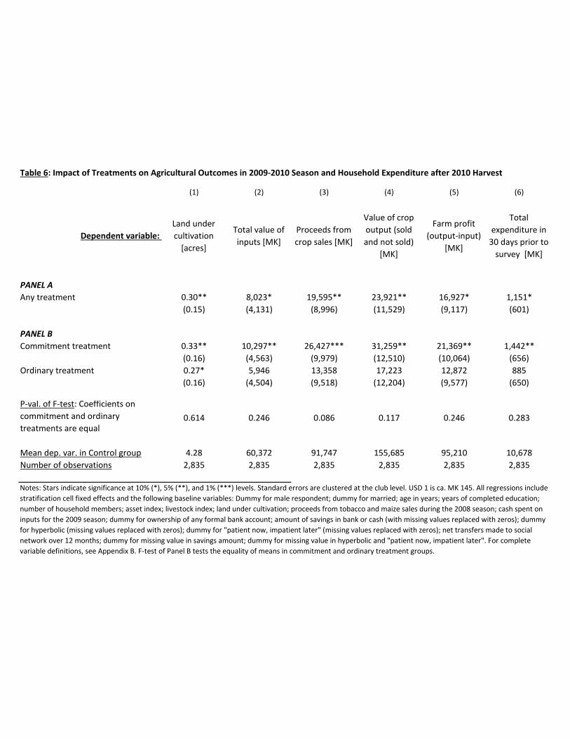
Table 6: Impact of Treatments on Agricultural Outcomes in 2009-2010 Season and Household Expenditure after 2010 Harvest
(1) (2) (3) (4) (5) (6)
Dependent variable:
Land under
cultivation
[acres]
Total value of
inputs [MK]
Proceeds from
crop sales [MK]
Value of crop
output (sold
and not sold)
[MK]
Farm profit
(output-input)
[MK]
Total
expenditure in
30 days prior to
survey [MK]
PANEL A
Any treatment 0.30** 8,023* 19,595** 23,921** 16,927* 1,151*
(0.15) (4,131) (8,996) (11,529) (9,117) (601)
PANEL B
Commitment treatment 0.33** 10,297** 26,427*** 31,259** 21,369** 1,442**
(0.16) (4,563) (9,979) (12,510) (10,064) (656)
Ordinary treatment 0.27* 5,946 13,358 17,223 12,872 885
(0.16) (4,504) (9,518) (12,204) (9,577) (650)
P-val. of F-test: Coefficients on
commitment and ordinary
treatments are equal0.614 0.246 0.086 0.117 0.246 0.283
Mean dep. var. in Control group 4.28 60,372 91,747 155,685 95,210 10,678
Number of observations 2,835 2,835 2,835 2,835 2,835 2,835
Notes: Stars indicate significance at 10% (*), 5% (**), and 1% (***) levels. Standard errors are clustered at the club level. USD 1 is ca. MK 145. All regressions include
stratification cell fixed effects and the following baseline variables: Dummy for male respondent; dummy for married; age in years; years of completed education;
number of household members; asset index; livestock index; land under cultivation; proceeds from tobacco and maize sales during the 2008 season; cash spent on
inputs for the 2009 season; dummy for ownership of any formal bank account; amount of savings in bank or cash (with missing values replaced with zeros); dummy
for hyperbolic (missing values replaced with zeros); dummy for "patient now, impatient later" (missing values replaced with zeros); net transfers made to social
network over 12 months; dummy for missing value in savings amount; dummy for missing value in hyperbolic and "patient now, impatient later". For complete
variable definitions, see Appendix B. F-test of Panel B tests the equality of means in commitment and ordinary treatment groups.

Table 7: Impact of treatments on household size, transfers and fixed deposit demand
(1) (2) (3) (4) (5) (6)
Dependent variable: Household sizeTobacco loan
amount [MK]
Total transfers
made [MK]
Total transfers
received [MK]
Total net
transfers made
[MK]
Has fixed
deposit
account
PANEL A
Any treatment 0.14 3,158 215 -301 477 0.032***
(0.09) (4,583) (249) (248) (322) (0.012)
PANEL B
Commitment treatment -0.004 3,418 304 -316 568 0.050***
(0.019) (4,897) (275) (258) (347) (0.014)
Ordinary treatment -0.010 2,920 134 -288 394 0.016
(0.019) (5,068) (267) (262) (342) (0.012)
P-val. of F-test: Coefficients on
commitment and ordinary
treatments are equal
0.748 0.899 0.431 0.856 0.483 0.008
Mean dep. var. in Control group 5.72 40,147 2,872 2,492 418 0.039
Number of observations 2,835 2,835 2,835 2,835 2,835 2,835
Notes: Stars indicate significance at 10% (*), 5% (**), and 1% (***) levels. Standard errors are clustered at the club level. USD 1 is ca. MK 145. All
regressions include stratification cell fixed effects and the following baseline variables: Dummy for male respondent; dummy for married; age in
years; years of completed education; number of household members; asset index; livestock index; land under cultivation; proceeds from tobacco
and maize sales during the 2008 season; cash spent on inputs for the 2009 season; dummy for ownership of any formal bank account; amount of
savings in bank or cash (with missing values replaced with zeros); dummy for hyperbolic (missing values replaced with zeros); dummy for "patient
now, impatient later" (missing values replaced with zeros); net transfers made to social network over 12 months; dummy for missing value in
savings amount; dummy for missing value in hyperbolic and "patient now, impatient later". For complete variable definitions, see Appendix B. F-test
of Panel B: "Commitment savings = Ordinary savings" tests the equality of means in commitment and ordinary treatment groups.

Appendix Table 1: Attrition from baseline to endline survey
Dependent variable: Not interviewed during endline survey
PANEL A
Any treatment -0.007
(0.018)
PANEL B
Commitment treatment -0.004
(0.019)
Ordinary treatment -0.010
(0.019)
P-val. of F-test: Commitment savings =
Ordinary savings0.619
PANEL C
Commitment, no raffle 0.002
(0.025)
Commitment, private raffle -0.006
(0.021)
Commitment, public raffle -0.006
(0.022)
Ordinary, no raffle -0.005
(0.025)
Ordinary, private raffle -0.037*
(0.021)
Ordinary, public raffle 0.010
(0.024)
P-val. of F-tests:
Commitment: priv. raffle vs. no raffle 0.717
Commitment: pub. raffle vs. no raffle 0.727
Ordinary: priv. raffle vs. no raffle 0.181
Ordinary: pub. raffle vs. no raffle 0.570
Mean dep. var. in Control group 0.099
Number of observations 3,150
Notes: Stars indicate significance at 10% (*), 5% (**), and 1% (***) levels. Standard errors are clustered at the club level. Regressions
include stratification cell fixed effects. Regression also includes the following baseline variables: Dummy for male respondent; dummy for
married; age in years; years of completed education; number of household members; asset index; livestock index; land under cultivation;
proceeds from tobacco and maize sales during the 2008 season; cash spent on inputs for the 2009 season; dummy for ownership of any
formal bank account; amount of savings in bank or cash (with missing values replaced with zeros); dummy for hyperbolic (missing values
replaced with zeros); dummy for "patient now, impatient later" (missing values replaced with zeros); net transfers made to social network
over 12 months; dummy for missing value in savings amount; dummy for missing value in hyperbolic and "patient now, impatient later".
For variable definitions, see Appendix B. F-test of Panel B: "Commitment savings = Ordinary savings" tests the equality of means in
commitment and ordinary treatment groups. F-tests of Panel C: "Commitment: priv. raffle vs. no raffle" tests the equality of means in
commitment treatment groups with private raffle and without raffle; similarly for the tests following below.
Appendix Table 2: Test of Balance in Baseline Characteristics (including raffle sub-treatments)
(1) (2) (3) (4) (5) (6) (7) (8) (9) (10) (11) (12) (13) (14) (15) (16) (17)
Dependent variable: Female MarriedAge
[years]
Years of
edu-
cation
House-
hold size
Asset
index
Live-
stock
index
Land
under
culti-
vation
[acres]
Pro-
ceeds
from crop
sales
[MK]
Cash
spent on
inputs
[MK]
Has bank
account
Savings in
accounts
and cash
[MK]
Hyper-
bolic
Patient
now, im-
patient
later
Net
transfers
made in
past 12m
[MK]
Missing
val.:
formal
savings
and cash
Missing
val.: time
prefe-
rences
Commitment, no raffle 0.035* -0.017 -1.17 0.38 -0.08 0.13 -0.02 -0.01 11,742 2,233 -0.042 770 0.029 -0.055 -314 -0.007 0.012
(0.019) (0.015) (1.09) (0.24) (0.16) (0.15) (0.12) (0.18) (13,191) (3,415) (0.045) (885) (0.025) (0.047) (541) (0.019) (0.010)
Commitment, private raffle 0.038** -0.009 -1.05 -0.01 0.21 0.17 -0.04 0.24 9,648 5,285* 0.010 460 0.035 -0.096** -162 0.015 -0.001
(0.018) (0.013) (1.10) (0.29) (0.16) (0.16) (0.12) (0.18) (11,700) (3,099) (0.041) (828) (0.026) (0.039) (558) (0.018) (0.006)
Commitment, public raffle 0.063*** -0.030** -1.94 -0.08 -0.25 -0.09 -0.12 -0.36** -4,403 2,360 -0.084** -75 0.009 -0.074* -113 -0.021 -0.003
(0.017) (0.014) (1.24) (0.28) (0.16) (0.13) (0.11) (0.17) (12,891) (3,231) (0.042) (712) (0.022) (0.044) (597) (0.017) (0.006)
Ordinary, no raffle 0.048*** -0.032** -0.93 0.03 -0.11 0.24 -0.04 0.11 7,888 2,316 0.014 200 0.003 -0.084* 82 -0.009 0.001
(0.016) (0.013) (1.25) (0.28) (0.16) (0.16) (0.10) (0.20) (12,765) (2,626) (0.042) (731) (0.021) (0.050) (547) (0.019) (0.008)
Ordinary, private raffle 0.048*** -0.002 -1.50 0.17 0.07 0.15 -0.05 -0.02 11,512 8,791** -0.005 199 0.003 -0.012 267 0.000 0.004
(0.018) (0.011) (1.20) (0.27) (0.16) (0.15) (0.10) (0.16) (11,298) (3,403) (0.039) (718) (0.022) (0.041) (591) (0.020) (0.008)
Ordinary, public raffle 0.031* -0.019 -1.90* 0.36 -0.02 -0.11 -0.10 -0.04 5,689 2,266 -0.023 714 -0.005 -0.006 604 0.008 -0.003
(0.017) (0.013) (1.07) (0.26) (0.15) (0.14) (0.10) (0.18) (12,461) (2,733) (0.042) (723) (0.020) (0.045) (541) (0.021) (0.005)
P-val. of F-tests:
Com.: priv. raffle vs. no raffle 0.894 0.637 0.903 0.141 0.054 0.809 0.833 0.186 0.879 0.436 0.278 0.760 0.816 0.324 0.760 0.306 0.208
Com.: pub. raffle vs. no raffle 0.178 0.460 0.494 0.061 0.247 0.156 0.322 0.049 0.269 0.975 0.407 0.342 0.450 0.685 0.709 0.511 0.123
Ord.: priv. raffle vs. no raffle 0.984 0.023 0.641 0.607 0.281 0.627 0.884 0.456 0.777 0.073 0.681 0.998 0.988 0.128 0.729 0.677 0.747
Ord.: pub. raffle vs. no raffle 0.366 0.366 0.376 0.220 0.543 0.024 0.443 0.427 0.872 0.986 0.448 0.482 0.686 0.125 0.275 0.469 0.609
P-values of F-tests for joint significance of baseline variables:
Commitment, no raffle 0.9279
Commitment, private raffle 0.3273
Commitment, public raffle 0.1738
Ordinary, no raffle 0.7313
Ordinary, private raffle 0.4927
Ordinary, public raffle 0.0993
Mean dep. var. in Control group 0.024 0.972 46.23 5.31 5.81 -0.11 0.03 4.67 117,495 21,798 0.658 3,235 0.095 0.352 1,655 0.066 0.009
Number of observations 3,150 3,150 3,150 3,150 3,150 3,150 3,150 3,150 3,150 3,150 3,150 2,949 3,117 3,117 3,150 3,150 3,150
Notes: Stars indicate significance at 10% (*), 5% (**), and 1% (***) levels. Standard errors are clustered at the club level. USD 1 is ca. MK 145. All regressions include stratification-cell fixed effects. For variable definitions, see
Appendix B. F-test of Panel B: "Commitment savings = Ordinary savings" tests the equality of means in commitment and ordinary treatment groups. F-tests of Panel C: "Commit.: priv. raffle vs. no raffle" tests the equality of
means in commitment treatment groups with private raffle and without raffle; similarly for the tests following below. F-tests of joint significance: test of joint significance in regression of respective treatment dummies on all 17
baseline variables.

Appendix Table 3: Impact of Treatments on Deposits and Withdrawals (including raffle sub-treatments)
(1) (2) (3) (4) (5) (6)
Dependent variable:
Any transfer
via direct
deposit
(take-up)
Total
deposits
into
accounts
[MK]
Deposits
into
ordinary
accounts
[MK]
Deposits
into commit-
ment
accounts
[MK]
Deposits
into other
accounts
[MK]
Total with-
drawals
from
accounts
[MK]
Time period:Mar 2009 -
Apr 2010
Mar-Oct
2009
Mar-Oct
2009
Mar-Oct
2009
Mar-Oct
2009
Mar-Oct
2009
Commitment, no raffle 0.214*** 21,861*** 19,464*** 1,994** 403 -20,740***
-0.046 (6,885) (6,282) (789) (348) (6,829)
Commitment, private raffle 0.245*** 16,529*** 15,011*** 1,295*** 223 -15,356***
-0.055 (5,744) (5,469) (484) (254) (5,425)
Commitment, public raffle 0.162*** 18,244*** 16,792*** 1,200*** 252 -16,671***
-0.049 (5,927) (5,786) (396) (217) (5,649)
Ordinary, no raffle 0.164*** 21,596*** 21,367*** -100 329 -20,968***
-0.049 (7,073) (6,962) (235) (278) (6,751)
Ordinary, private raffle 0.170*** 6,977 7,233 -99 -157 -6,002
-0.05 (4,843) (4,709) (231) (162) (4,762)
Ordinary, public raffle 0.209*** 20,898*** 21,148*** -54 -196 -21,158***
-0.055 (7,941) (7,875) (212) (161) (7,941)
P-val. of F-tests:
Commit.: priv. raffle vs. no raffle 0.590 0.497 0.536 0.444 0.623 0.476
Commit.: pub. raffle vs. no raffle 0.313 0.655 0.724 0.351 0.670 0.606
Ordinary: priv. raffle vs. no raffle 0.916 0.048 0.053 0.996 0.074 0.034
Ordinary: pub. raffle vs. no raffle 0.439 0.940 0.981 0.839 0.042 0.983
Mean dep. var. in Control group 0.000 3,281 3,107 0 174 -3,256
Number of observations 3,150 3,150 3,150 3,150 3,150 3,150
Notes: Stars indicate significance at 10% (*), 5% (**), and 1% (***) levels. Standard errors are clustered at the club level. USD 1 is ca. MK 145. All
regressions include stratification cell fixed effects and the following baseline variables: Dummy for male respondent; dummy for married; age in years;
years of completed education; number of household members; asset index; livestock index; land under cultivation; proceeds from tobacco and maize
sales during the 2008 season; cash spent on inputs for the 2009 season; dummy for ownership of any formal bank account; amount of savings in bank or
cash (with missing values replaced with zeros); dummy for hyperbolic (missing values replaced with zeros); dummy for "patient now, impatient later"
(missing values replaced with zeros); net transfers made to social network over 12 months; dummy for missing value in savings amount; dummy for
missing value in hyperbolic and "patient now, impatient later". For complete variable definitions, see Appendix B. F-test of Panel B: "Commitment savings
= Ordinary savings" tests the equality of means in commitment and ordinary treatment groups. F-tests of Panel C: "Commitment: priv. raffle vs. no raffle"
tests the equality of means in commitment treatment groups with private raffle and without raffle; similarly for the tests following below. Planting season
is Nov-Apr. Fertilizer application occurs in Nov-Dec. Fertilizer purchases occur in both pre-planting period (Oct and before) and start of planting season
(Nov-Dec).

Appendix Table 4: Impact of Treatments on Savings Balances (including raffle sub-treatments)
Ordinary least-squares regressions
(1) (2) (3) (4)
Dependent variable:
Account type: All accounts, in total Ordinary Commitment Other
Commitment, no raffle 2,475*** 621* 1,142*** 711*
(775) (359) (434) (428)
Commitment, private raffle 2,074*** 1,112** 892** 69
(772) (528) (372) (137)
Commitment, public raffle 2,893*** 1,762*** 777*** 354
(789) (676) (295) (302)
Ordinary, no raffle 1,866** 1,702** -37 200
(798) (688) (168) (201)
Ordinary, private raffle 973* 722* -56 307
(520) (409) (171) (247)
Ordinary, public raffle 1,071* 1,065** 20 -14
(600) (521) (153) (107)
P-val. of F-tests:
Commit.: priv. raffle vs. no raffle 0.700 0.397 0.660 0.153
Commit.: pub. raffle vs. no raffle 0.680 0.105 0.453 0.489
Ordinary: priv. raffle vs. no raffle 0.323 0.223 0.920 0.724
Ordinary: pub. raffle vs. no raffle 0.389 0.447 0.740 0.273
Mean dep. var. in Control group 364 302 0 62
Number of observations 3,150 3,150 3,150 3,150
Savings balance immediately prior to planting period (on Oct 22, 2009)
Notes: Stars indicate significance at 10% (*), 5% (**), and 1% (***) levels. Dependent variable is savings balance on Oct 22, 2009, just prior to
November-December 2009 planting season. Standard errors are clustered at the club level. USD 1 is ca. MK 145. All regressions include
stratification cell fixed effects and the following baseline variables: Dummy for male respondent; dummy for married; age in years; years of
completed education; number of household members; asset index; livestock index; land under cultivation; proceeds from tobacco and maize sales
during the 2008 season; cash spent on inputs for the 2009 season; dummy for ownership of any formal bank account; amount of savings in bank
or cash (with missing values replaced with zeros); dummy for hyperbolic (missing values replaced with zeros); dummy for "patient now, impatient
later" (missing values replaced with zeros); net transfers made to social network over 12 months; dummy for missing value in savings amount;
dummy for missing value in hyperbolic and "patient now, impatient later". For complete variable definitions, see Appendix B. F-tests:
"Commitment: priv. raffle vs. no raffle" tests the equality of means in commitment treatment groups with private raffle and without raffle;
similarly for the tests following below. Planting season is Nov-Apr. Fertilizer application occurs in Nov-Dec.

Appendix Table 5: Impact of Treatments on Agricultural Outcomes in 2009-2010 Season and Household Expenditure after 2010 Harvest
(including raffle sub-treatments)
(1) (2) (3) (4) (5) (6)
Dependent variable:
Land under
cultivation
[acres]
Total value of
inputs [MK]
Proceeds from
crop sales [MK]
Value of crop
output (sold and
not sold) [MK]
Farm profit
(output-input)
[MK]
Total
expenditure in
30 days prior to
survey [MK]
Commitment, no raffle 0.42** 16,534** 22,963** 33,968** 19,205 1,860**
(0.20) (6,394) (11,614) (15,115) (12,399) (857)
Commitment, private raffle 0.29 8,026 34,667** 33,031** 22,252* 1,328*
(0.19) (6,068) (13,683) (15,914) (13,064) (799)
Commitment, public raffle 0.28 6,645 21,158* 26,690* 22,436* 1,151
(0.20) (5,390) (12,114) (14,929) (12,011) (907)
Ordinary, no raffle 0.05 8,521 10,306 7,844 1,888 413
(0.19) (6,273) (11,935) (14,806) (11,195) (876)
Ordinary, private raffle 0.30 1,184 10,720 17,331 17,260 691
(0.21) (5,473) (11,717) (15,151) (12,048) (849)
Ordinary, public raffle 0.47** 8,408 18,928 26,528* 19,323 1,568**
(0.19) (5,686) (12,156) (15,218) (12,323) (795)
P-val. of F-tests:
Commit.: priv. raffle vs. no raffle 0.478 0.239 0.396 0.953 0.821 0.550
Commit.: pub. raffle vs. no raffle 0.476 0.133 0.880 0.622 0.791 0.470
Ordinary: priv. raffle vs. no raffle 0.229 0.265 0.973 0.532 0.191 0.777
Ordinary: pub. raffle vs. no raffle 0.032 0.987 0.495 0.217 0.143 0.216
Mean dep. var. in Control group 4.28 60,372 91,747 155,685 95,210 10,678
Number of observations 2,835 2,835 2,835 2,835 2,835 2,835
Notes: Stars indicate significance at 10% (*), 5% (**), and 1% (***) levels. Standard errors are clustered at the club level. USD 1 is ca. MK 145. All regressions
include stratification cell fixed effects and the following baseline variables: Dummy for male respondent; dummy for married; age in years; years of completed
education; number of household members; asset index; livestock index; land under cultivation; proceeds from tobacco and maize sales during the 2008 season;
cash spent on inputs for the 2009 season; dummy for ownership of any formal bank account; amount of savings in bank or cash (with missing values replaced
with zeros); dummy for hyperbolic (missing values replaced with zeros); dummy for "patient now, impatient later" (missing values replaced with zeros); net
transfers made to social network over 12 months; dummy for missing value in savings amount; dummy for missing value in hyperbolic and "patient now,
impatient later". For complete variable definitions, see Appendix B. F-tests: "Commitment: priv. raffle vs. no raffle" tests the equality of means in commitment
treatment groups with private raffle and without raffle; similarly for the tests following below.

Appendix Table 6: Impact of treatments on household size, transfers and fixed deposit demand
(including raffle sub-treatments)
(1) (2) (3) (4) (5) (6)
Dependent variable: Household sizeTotal transfers
made [MK]
Total transfers
received [MK]
Total net
transfers made
[MK]
Tobacco loan
amount [MK]
Has fixed
deposit account
Commitment, no raffle 0.06 278 -490* 724* 3,686 0.062***
(0.11) (331) (290) (405) (5,706) (0.024)
Commitment, private raffle 0.18 375 -484 845* 7,471 0.040**
(0.12) (378) (298) (434) (6,601) (0.017)
Commitment, public raffle 0.13 257 28 131 -1,053 0.049**
(0.11) (332) (301) (410) (5,897) (0.019)
Ordinary, no raffle 0.05 491 -206 642 4,508 0.033**
(0.11) (352) (322) (436) (6,809) (0.017)
Ordinary, private raffle 0.18 -66 -251 196 -649 -0.000
(0.11) (296) (314) (422) (6,282) (0.013)
Ordinary, public raffle 0.21* -20 -407 345 4,930 0.018
(0.11) (345) (307) (385) (6,465) (0.016)
P-val. of F-tests:
Commit.: priv. raffle vs. no raffle 0.279 0.799 0.981 0.764 0.564 0.389
Commit.: pub. raffle vs. no raffle 0.497 0.949 0.045 0.138 0.410 0.624
Ordinary: priv. raffle vs. no raffle 0.249 0.097 0.886 0.315 0.474 0.037
Ordinary: pub. raffle vs. no raffle 0.134 0.171 0.500 0.460 0.955 0.432
Mean dep. var. in Control group 5.72 2,872 2,492 418 40,147 0.039
Number of observations 2,835 2,835 2,835 2,835 2,835 2,835
Notes: Stars indicate significance at 10% (*), 5% (**), and 1% (***) levels. Standard errors are clustered at the club level. USD 1 is ca. MK 145. All regressions
include stratification cell fixed effects and the following baseline variables: Dummy for male respondent; dummy for married; age in years; years of
completed education; number of household members; asset index; livestock index; land under cultivation; proceeds from tobacco and maize sales during the
2008 season; cash spent on inputs for the 2009 season; dummy for ownership of any formal bank account; amount of savings in bank or cash (with missing
values replaced with zeros); dummy for hyperbolic (missing values replaced with zeros); dummy for "patient now, impatient later" (missing values replaced
with zeros); net transfers made to social network over 12 months; dummy for missing value in savings amount; dummy for missing value in hyperbolic and
"patient now, impatient later". For complete variable definitions, see Appendix B. F-tests: "Commitment: priv. raffle vs. no raffle" tests the equality of means
in commitment treatment groups with private raffle and without raffle; similarly for the tests following below.

Appendix Table 7: Take-up as a function of baseline characteristics
(1) (2) (3) (4)
Dependent variable: Any active account
with OBM
Any transfer via direct
deposit
Any active account
with OBM
Any transfer via direct
deposit
Female -0.013 0.023 -0.049 0.023
(0.029) (0.023) (0.037) (0.031)
Married -0.027 -0.032 -0.028 -0.038
(0.043) (0.037) (0.061) (0.055)
Age [years] 0.000 0.001* 0.000 0.002***
(0.001) (0.001) (0.001) (0.001)
Years of education 0.009*** 0.007*** 0.009*** 0.008**
(0.003) (0.002) (0.003) (0.003)
Household size 0.004 0.006* 0.002 0.003
(0.004) (0.003) (0.006) (0.004)
Asset index 0.003 0.001 -0.013 -0.014**
(0.007) (0.006) (0.009) (0.007)
Livestock index 0.008 -0.003 0.006 0.006
(0.009) (0.007) (0.010) (0.008)
Land under culti-vation [acres] 0.007 0.005 0.009 0.005
(0.006) (0.005) (0.007) (0.005)
Has bank account 0.222*** 0.059*** 0.227*** 0.062**
(0.026) (0.018) (0.039) (0.029)
Savings in accounts and cash [MK10,000] -0.008 -0.004 0.008 -0.010
(0.009) (0.006) (0.015) (0.009)
Hyperbolic -0.007 0.007 -0.037 -0.001
(0.028) (0.024) (0.035) (0.027)
Patient now, impatient later -0.015 -0.016 -0.018 -0.033
(0.020) (0.016) (0.029) (0.028)
Cash spent on inputs [MK10,000] -0.005* -0.001 -0.001 0.001
(0.003) (0.002) (0.004) (0.003)
Proceeds from crop sales [MK10,000] 0.002** 0.001 -0.000 0.001
(0.001) (0.001) (0.001) (0.001)
Net transfers made in past 12m [MK10,000] 0.017 0.016* 0.009 0.017
(0.011) (0.009) (0.014) (0.012)
Mean dep. var. 0.335 0.178 0.319 0.177
Number of observations 2,726 2,726 1,314 1,314
R-squared 0.258 0.237 0.316 0.289
Orindary and Commitment treatment
observations onlyCommitment treatment observations only
Notes: Stars indicate significance at 10% (*), 5% (**), and 1% (***) levels. Standard errors are clustered at the club level. USD 1 is ca. MK 145. "Any active account with
OBM" is 1 if the respondent had an active account with OBM (active means all steps of account registration were completed including payment of opening fee, and
balance exceeds minimum if applicable) when data was provided on Oct 22, 2009, and 0 if not. "Any transfer via direct deposit" is the same outcome variable as in Table 4
and defined as 1 if the respondent receives any deposit from his or her tobacco club’s account to his or her individual savings account, and 0 if not. All regressions include
stratification cell fixed effects. Missing values for hyperbolic dummy, for dummy "patient now, impatient later" and for savings in accounts and cash have been replaced
with zeros and dummies for missing value are included as controls. For readability, monetary variables are defined in units of MK10,000. For further variable definitions,
see Appendix B.