f73db3 categorical data analysis workbook contents page preface aims summary...
TRANSCRIPT

F73DB3 CATEGORICAL DATA ANALYSIS
Workbook
Contents pagePreface
AimsSummaryContent/structure/syllabusplus other information
Background – computing (R)
hwu

Examples
Single classifications (1-13)
Two-way classifications (14-27)
Three-way classifications (28-32)
hwu

hwu
Example 1 Eye colours
Colour A B C D
Frequency observed 89 66 60 85

hwu
Example 2 Prussian cavalry deaths
(a)Numbers killed in each unit in each year - frequency table
Number killed
0 1 2 3 4 5
Total
Frequency observed
144 91 32 11 2 0 280

hwu
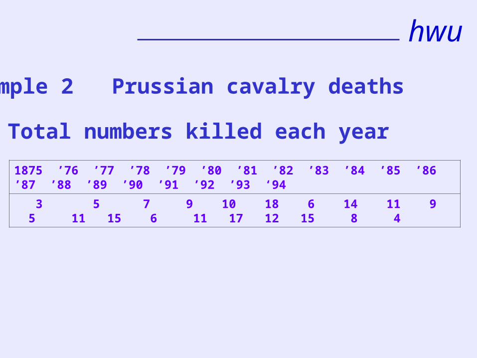
Example 2 Prussian cavalry deaths
(b) Numbers killed in each unit in each year – raw data
0 0 1 0 0 2 0 0 0 0 . . . . . . . . . . . . . . . . . . . . . . . 00 0 2 0 1 0 1 2 0 1 . . . . . . . . . . . . . . . . . . . . . . . .0…..…..3 0 0 1 0 0 2 1 0 0 1 0 0 1 0 0 1 1 2 0 1 0 1 1
hwu
Example 2 Prussian cavalry deaths
(c) Total numbers killed each year
1875 ’76 ’77 ’78 ’79 ’80 ’81 ’82 ’83 ’84 ’85 ’86 ’87 ’88 ’89 ’90 ’91 ’92 ’93 ‘94
3 5 7 9 10 18 6 14 11 9 5 11 15 6 11 17 12 15 8 4

hwu
Example 4 Political views
1 2 3 4 5 6 7 (very L) (centre) (very R)
Don’tKnow
Total
46 179 196 559 232 150 35 93 1490

hwu
Example 7 Vehicle repair visits
Number of visits 0 1 2 3 4 5 6 Total
Frequency observed
295 190 53 5 5 2 0 550

hwu
Example 15 Patients in clinical trial
Drug Placebo Total
Side-effects 15 4 19
No side-effects 35 46 81
Total 50 50 100

§1 INTRODUCTION
Data are counts/frequencies (not measurements)
Categories (explanatory variable)
Distribution in the cells (response)
Frequency distribution
Single classifications
Two-way classifications
hwu
hwu
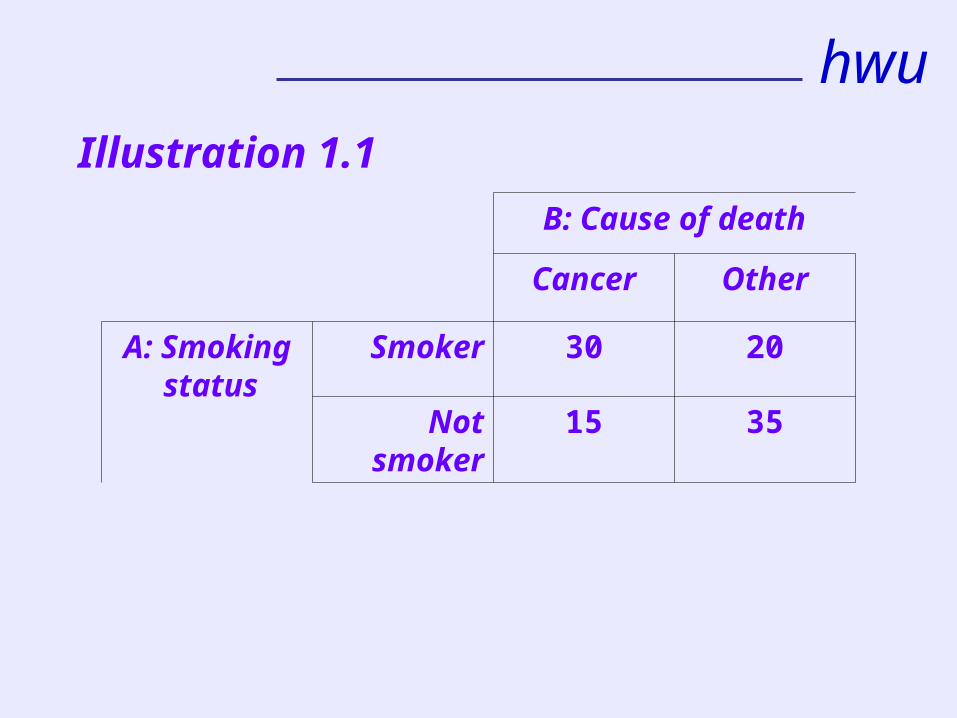
B: Cause of death
Cancer Other
A: Smoking status
Smoker 30 20
Not smoker 15 35
Illustration 1.1

Data may arise as
Bernoulli/binomial data (2 outcomes)
Multinomial data (more than 2 outcomes)
Poisson data
[+ Negative binomial data – the version with
range x = 0,1,2, …]
hwu

hwu
§2 POISSON PROCESS AND
ASSOCIATED DISTRIBUTIONS

hwu2.1 Bernoulli trials and related distributions
Number of successes – binomial distribution
[Time before kth success – negative binomial distributionTime to first success – geometric distribution]
Conditional distribution of success times

hwu
2.2 Poisson process and related distributions
time
hwu
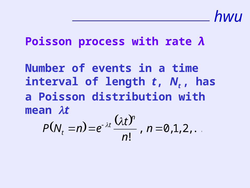
Poisson process with rate λ
Number of events in a time interval of length t, Nt , has a Poisson distribution with mean t
...,2,1,0,
! n
n
tenNP
nt
t

hwu
Poisson process with rate λ
Inter-event time, T, has an exponential distribution with parameter (mean 1/)
, 0tf t e t

hwu
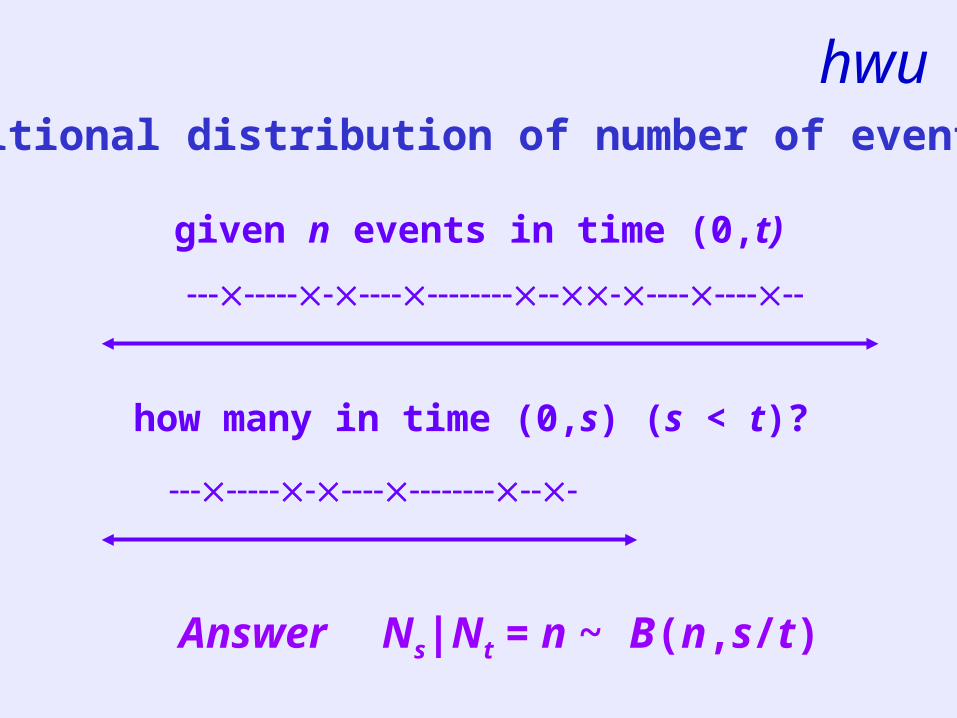
given n events in time (0,t)
how many in time (0,s) (s < t)?
Conditional distribution of number of events
hwu
given n events in time (0,t)
how many in time (0,s) (s < t)?
Conditional distribution of number of events
Answer Ns|Nt = n ~ B(n,s/t)

hwu
Splitting into subprocesses
time

hwu
0 10 20 30 40 50
02
04
06
08
01
00
t
N
Realisation of a Poisson process
# events
time
hwu
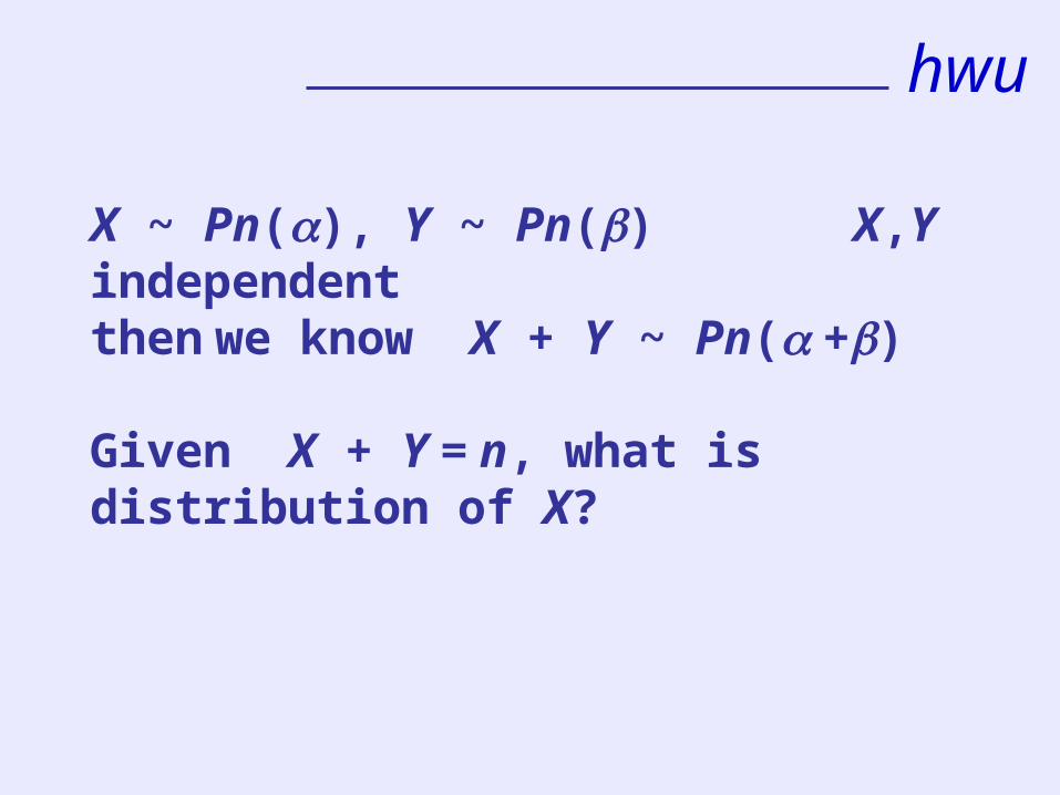
X ~ Pn(), Y ~ Pn() X,Y independentthen we know X + Y ~ Pn( +)
Given X + Y = n, what is distribution of X?

hwu
X ~ Pn(), Y ~ Pn() X,Y independentthen we know X + Y ~ Pn(+)
Given X + Y = n, what is distribution of X?
AnswerX|X+Y=n ~ B(n,p) where p = /( +)
hwu
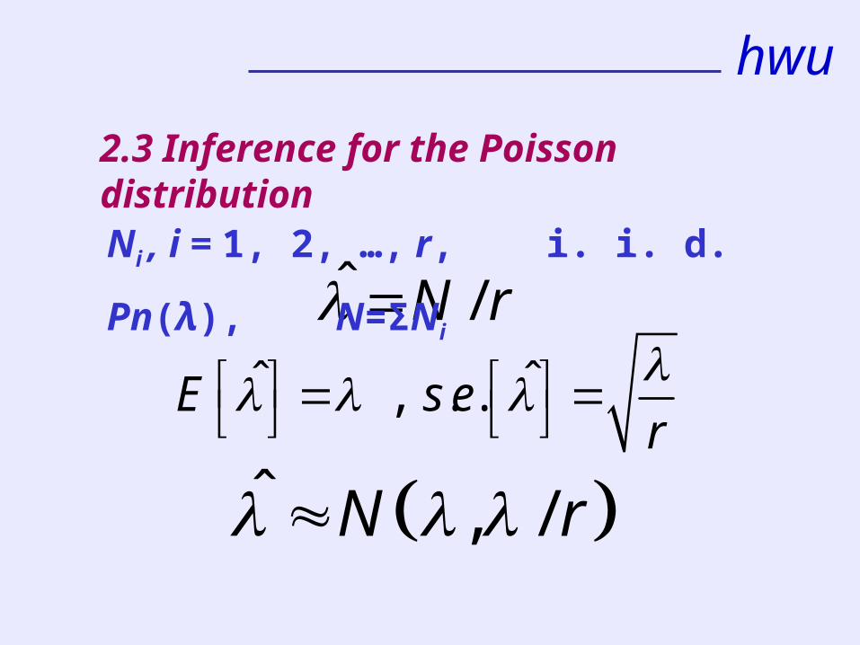
2.3 Inference for the Poisson distribution
ˆ /N r ˆ ˆ, . .E s e
r
ˆ , /N r
Ni , i = 1, 2, …, r, i. i. d. Pn(λ), N=ΣNi
hwu
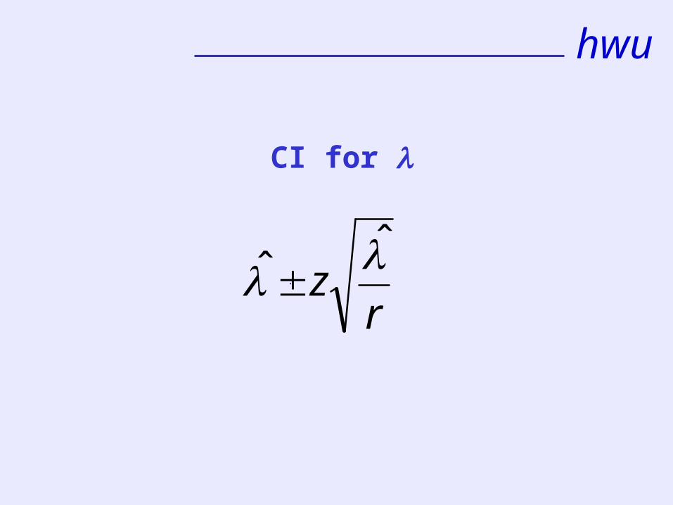
CI for
rz
ˆ
ˆ .

hwu
2.4 Dispersion and LR tests for Poisson dataHomogeneity hypothesis
H0: the Ni s are i. i. d. Pn()
(for some unknown)
2
2 211
r
ii
r
N MX
M
Dispersion statistic
(M = sample mean)

hwu
Likelihood ratio statistic
22
12 log /i i r
Y N N M
form for calculation – see p18 ◄◄
hwu
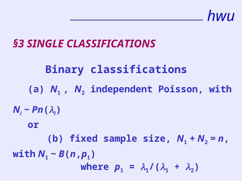
§3 SINGLE CLASSIFICATIONS
Binary classifications
(a) N1 , N2 independent Poisson, with Ni ~ Pn(i)
or
(b) fixed sample size, N1 + N2 = n, with N1 ~ B(n,p1) where p1 = 1/(1 + 2)
hwu
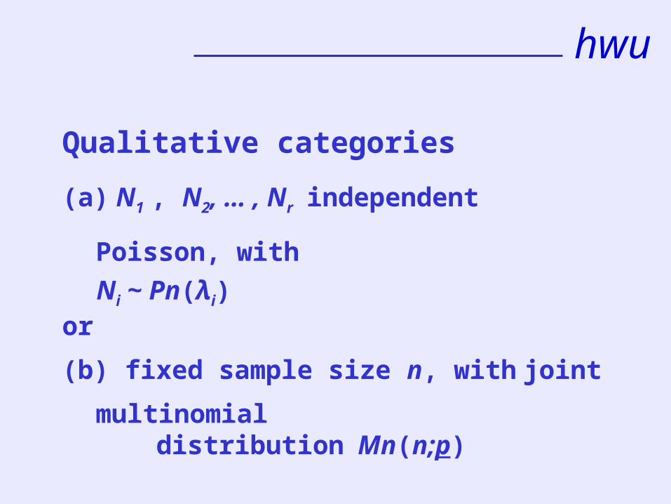
Qualitative categories
(a) N1 , N2, … , Nr independent Poisson, with
Ni ~ Pn(λi) or
(b) fixed sample size n, with joint multinomial distribution Mn(n;p)
hwu
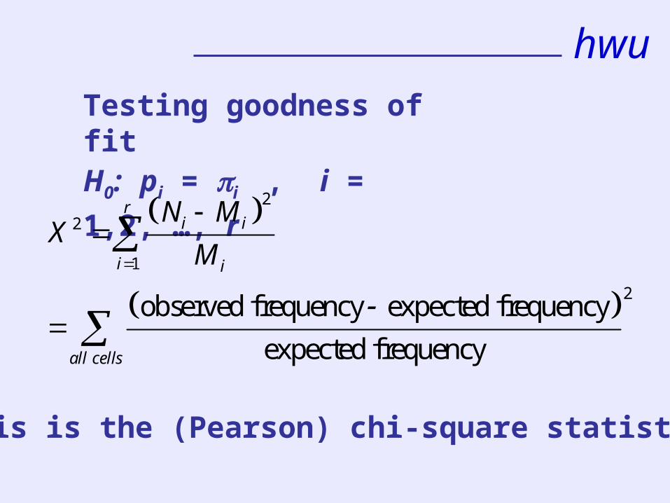
Testing goodness of fitH0: pi = i , i = 1,2, …, r
2
2
1
2observed frequency expected frequency
expected frequency
ri i
i i
all cells
N MX
M
This is the (Pearson) chi-square statistic

hwu
2O E
E
2observed frequency expected frequency
expected frequency
The statistic often appears as
hwu
21
21
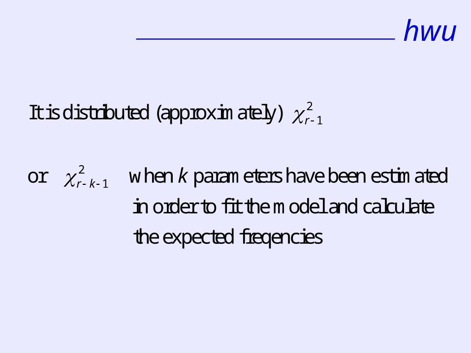
It is distributed (approximately)
or when parameters have been estimated
in order to fit the model and calculate
the expected freqencies
r
r k k
hwu
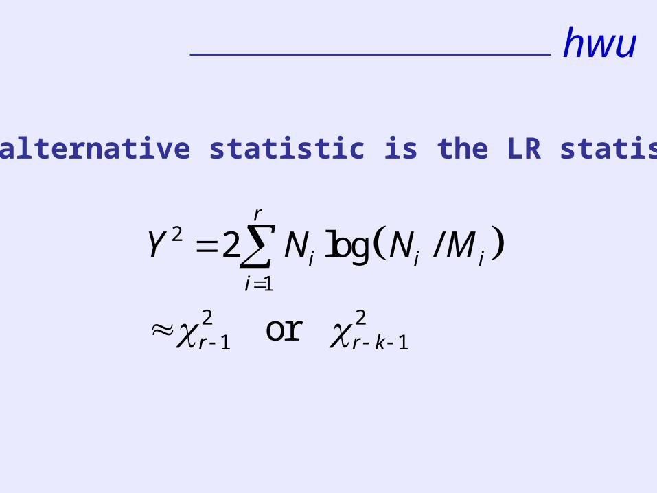
An alternative statistic is the LR statistic
2
1
2 21 1
2 log /
or
r
i i ii
r r k
Y N N M

hwu
Sparse data/small expected frequencies
ensure mi 1 for all cells, and
mi 5 for at least about 80% of the cells
if not - combine adjacent cells sensibly

hwu
Goodness-of-fit tests for frequency distributions
- very well-known application of the
2observed frequency expected frequency
expected frequencyall cells
statistic (see Illustration 3.4 p 22/23)
hwu
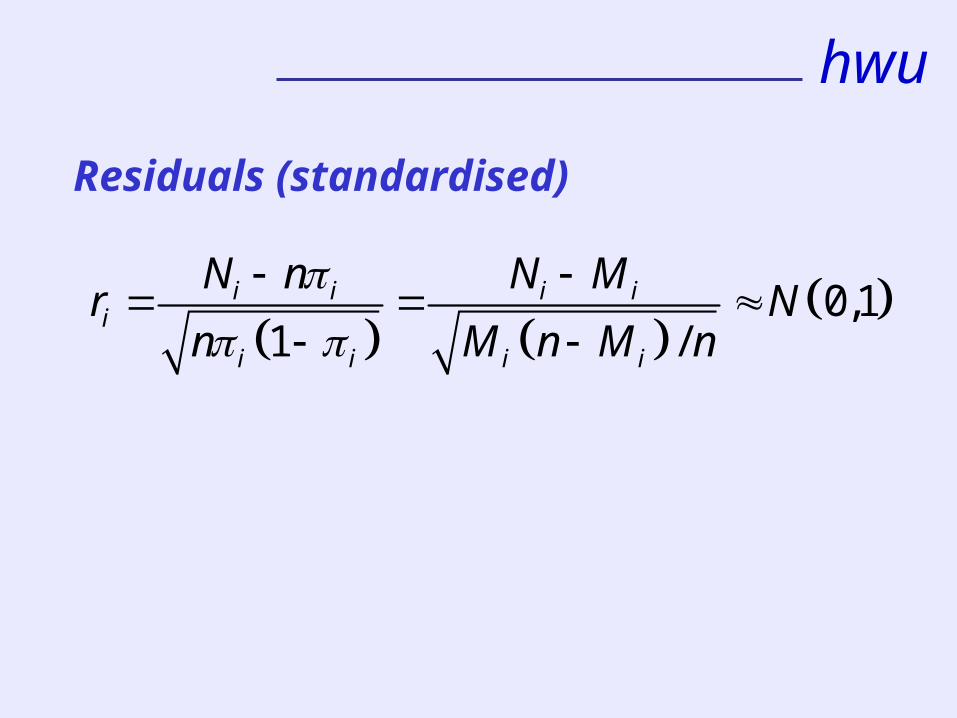
Residuals (standardised)
0,1
1 /i i i i
i
i i i i
N n N Mr N
n M n M n

hwu
Residuals (standardised)
0,1
1 /i i i i
i
i i i i
N n N Mr N
n M n M n
0,1i ii
i
N Mr N
M
simpler version

hwu
Number of papers per author 1 2 3 4 5 6 7 8 9 10 11Number of authors 1062 263 120 50 22 7 6 2 0 1 1
MAJOR ILLUSTRATION 1Publish and be modelled
, 1, 2, 3,...!
x
P X x xx
Model

hwu
MAJOR ILLUSTRATION 2Birds in hedges
Hedge type i A B C D E F GHedge length (m) li 2320 2460 2455 2805 2335 2645 2099Number of pairs ni 14 16 14 26 15 40 71
Model Ni ~ Pn(ili)

hwu
Example 14 Numbers of mice bearing tumours in treated and control groups
Treated Control Total
Tumours 4 5 9
No tumours 12 74 86
Total 16 79 95
§4 TWO-WAY CLASSIFICATIONS

hwu
Example 15 Patients in clinical trial
Drug Placebo Total
Side-effects 15 4 19
No side-effects 35 46 81
Total 50 50 100

hwu
Patients in clinical trial – take 2
Drug Placebo Total
Side-effects 15 15 30
No side-effects 35 35 70
Total 50 50 100
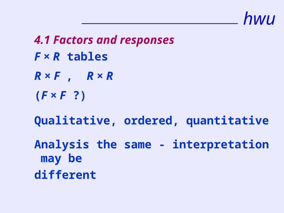
4.1 Factors and responses
F × R tables
R × F , R × R
(F × F ?)
Qualitative, ordered, quantitative
Analysis the same - interpretation may be
different
hwu

A two-way table is often called a
“contingency table”
(especially in R R case).
hwu

hwu
Exposed Not exposed Total
Disease n11 n12 n1●
No disease n21 n22 n2●
Total n●1 n●2 n●● = n
Notation (2 2 case, easily extended)
hwu
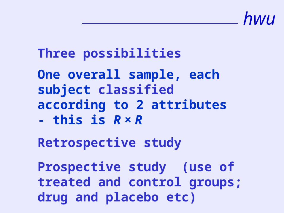
Three possibilities
One overall sample, each subject classified according to 2 attributes- this is R × R
Retrospective study
Prospective study (use of treated and control groups; drug and placebo etc)

hwu
(a) R × R case
(a1) Nij ~ Pn(ij) , independent
or, with fixed table total
(a2) Condition on n = nij :
N|n ~ Mn(n ; p)
where N = {Nij} , p = {pij}.
4.2 Distribution theory and tests for r × s tables
hwu
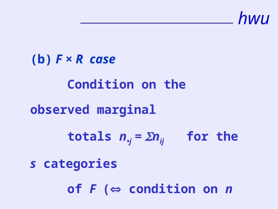
(b) F × R case
Condition on the observed marginal
totals n•j = nij for the s categories
of F ( condition on n and n•1)
s independent multinomials

hwu
Usual hypotheses
(a1) Nij ~ Pn(ij) , independent
H0: variables/responses are independent
ij = i• •j / •• = ki•
(a2) Multinomial data (table total fixed)
H0: variables/responses are independent
P(row i and column j) = P(row i)P(column j)

hwu
(b) Condition on n and n•j (fixed column totals)
Nij ~ Bi(n•j , pij) j = 1,2, …, s ; independent
H0: response is homogeneous (pij = pi• for all j)
i.e. response has the same distribution for all levels of the factor

hwu
2
2
??
ij ij
ij
N m
m
where mij = ni• n•j /n as before
Tests of H0
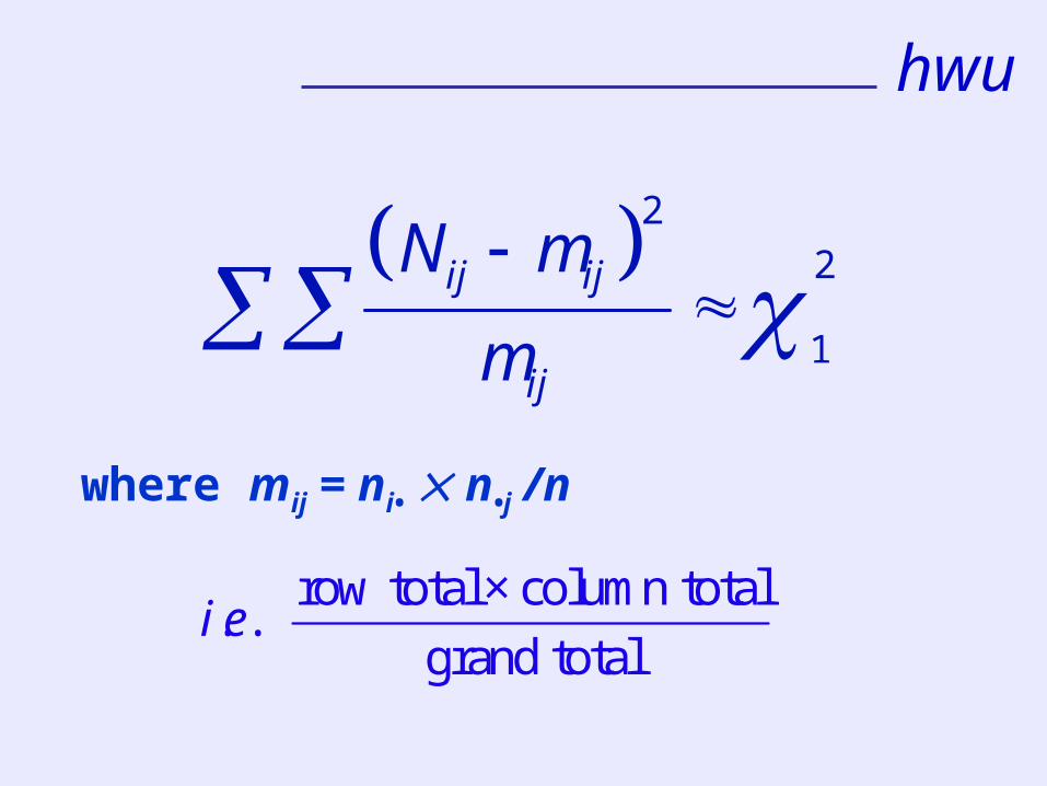
The χ2 (Pearson) statistic:

hwu
2
2
1 1
ij ij
r sij
N m
m
where mij = ni• n•j /n as before
Tests of H0
The χ2 (Pearson) statistic:

hwu
OR: test based on the LR statistic Y2
Illustration: tonsils data – see p27
In R
Pearson/X2 : read data in using “matrix”then use “chisq.test”
LR Y2 : calculate it directly (or get it fromthe results of fitting a “log-linear model”- see later)

hwu
Statistical tests
(a) Using Pearson’s χ2
4.3 The 2 2
table
Drug Placebo Total
Side-effects 15 4 19
No side-effects 35 46 81
Total 50 50 100
hwu
2
2
1
ij ij
ij
N m
m
where mij = ni• n•j /n
row total × column total. .
grand totali e
hwu
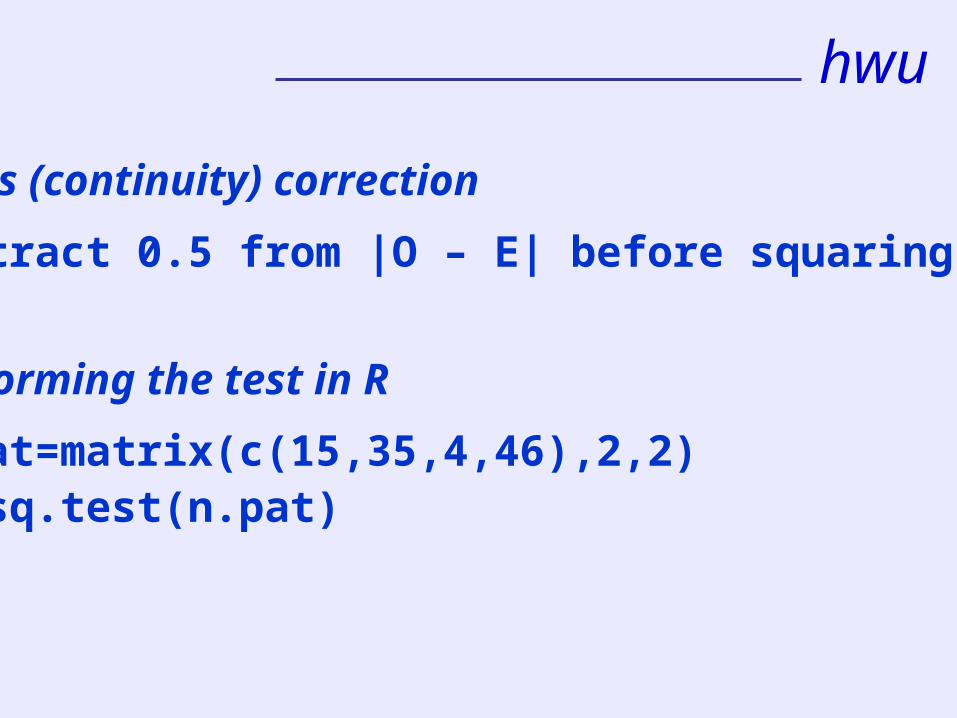
Yates (continuity) correction
Subtract 0.5 from |O – E| before squaring it
Performing the test in R
n.pat=matrix(c(15,35,4,46),2,2)chisq.test(n.pat)

hwu
(b) Using deviance/LR statistic Y2
(c) Comparing binomial probabilities
(d) Fisher’s exact test

hwu
Drug Placebo Total
Side-effects 15 4 N
19
No side-effects 35 46 81
Total 50 50 100

hwu
Under a random allocation
50 50
4 15 50!50!19!81!( 4) 0.0039
100 4!46!15!35!100!
19
P N
:!
product of marginal factorialsNote probability
n product of cell factorials
one-sided P-value = P(N 4) = 0.0047

hwu
In the 2 2 table, the H0 : independence
condition is equivalent to 1122 = 1221
Let λ = log(1122 /1221)
Then we have H0: λ = 0
λ is the “log odds ratio”
4.4 Log odds, combining and collapsing tables,interactions

hwu
The “λ = 0” hypothesis is often called the “no association” hypothesis.

hwu
The odds ratio is
1122 /1221
11 1 21 111 22 11 21
12 21 12 22 12 2 22 2
/ / //
/ / / /
n n n nn n n n
n n n n n n n n
1
2
( / )
odds on for column
odds on for column
odds ratio observed sample version
Sample equivalent is

hwu
The odds ratio (or log odds ratio) provides a measure of association for the factors in the table.
no association odds ratio = 1 log odds ratio = 0

hwu
Don’t combine heterogeneous
tables!

hwu
Interaction
An interaction exists between two factorswhen the effect of one factor is different at different levels of another factor.

hwu
45 50 55 60
0.0
00
0.0
02
0.0
04
0.0
06
0.0
08
0.0
10
0.0
12
age
d.r
ate

hwu
45 50 55 60
0.0
00
0.0
02
0.0
04
0.0
06
0.0
08
0.0
10
0.0
12
age
d.r
ate

hwu§5 INTRODUCTION TO GENERALISED LINEAR MODELS (GLMs)
Normal linear model
Y|x ~ N with E[Y|x]= + xor E[Y|x]= 0 + 1x1 + 2x2 + … + rxr = x
i.e. E[Y|x] = (x) = x

hwu
We are explaining (x) using a linear predictor (a linear function of the explanatory data)
Generalised linear model
Now we set g((x)) = x for some function g
We explain g((x)) using a linear function of the explanatory data, where g is called the link function

hwue.g. modelling a Poisson mean we use alog link g() = log
We use a linear predictor to explain log
rather than itself : the model is
Y|x ~ Pn with mean λx
with log λx = + x
or log λx = x
This is a log-linear model

hwu
An example is a trend model in which we uselogi = + i
Another example is a cyclic model in which we use
logi =0 + 1 cosθi + 2 sinθi

hwu
§6 MODELS FOR SINGLE CLASSIFICATIONS
6.1 Single classifications - trend models
Data: numbers in r categories
Model: Ni , i = 1, 2, …, r,
independent Pn(λi)

hwuBasic case
H0: λi’s equal v H1: λi’s follow a trend
Let Xj be category of observation j
P(Xj = i) = 1/r
XTest based on
see Illustration 6.1
hwu
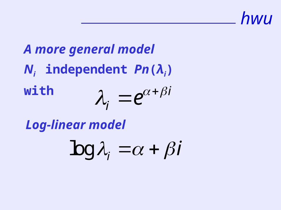
A more general model
Ni independent Pn(λi) with
ii e
log i i Log-linear model

hwu
It is a linear regression model for logλi
and a non-linear regression model for λi .
It is a generalised linear model.
Here the link between the parameter we are
estimating and the linear estimator is the
log function - it is a “log link”.

hwu
Fitting in R Example 13: stressful events data
>n=c(15,11, …, 1, 4) >r=length(n)>i=1:r

hwu
>n=c(15,11, …, 1, 4) response vector>r=length(n)>i=1:r explanatory vector
model>stress=glm(n~i,family=poisson)

hwu>summary(stress)
Call:glm(formula = n ~ i, family = poisson) model being fittedDeviance Residuals: Min 1Q Median 3Q Max -1.9886 -0.9631 0.1737 0.5131 2.0362 summary information on the residualsCoefficients: Estimate Std. Error z value Pr(>|z|) (Intercept) 2.80316 0.14816 18.920 < 2e-16 ***i -0.08377 0.01680 -4.986 6.15e-07 *** information on the fitted parameters

hwu
Signif. codes: 0 `***' 0.001 `**' 0.01 `*' 0.05 `.' 0.1 ` ' 1 (Dispersion parameter for poisson family taken to be 1)
Null deviance: 50.843 on 17 degrees of freedom Residual deviance: 24.570 on 16 degrees of freedom deviances (Y2 statistics)
AIC: 95.825Number of Fisher Scoring iterations: 4

hwu
Fitted mean is
ˆ exp 2.80316 0.08377i i
e.g. for date 6, i = 6 and fitted mean is exp(2.30054) = 9.980

hwuFitted model
5 10 15
0
5
10
15
Date
log-linear trend model for stress data
num
be
r

hwu
Test of H0: no trend the null fit, all fitted values equal (to theobserved mean) Y2 = 50.84 (~ 2 on 17df)
The trend model fitted values exp(2.80316-0.08377i)Y2 = 24.57 (~ 2 on 16df)
Crude 95% CI for slope is -0.084 ± 2(0.0168) i.e. -0.084 ± 0.034

hwu
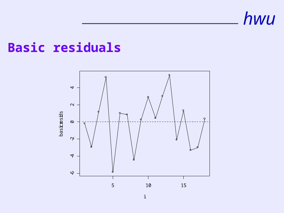
The lower the value of the residual deviance, the better in general is the fit of the model.
hwu
Basic residuals
5 10 15
-6-4
-20
24
i
ba
sicr
esi
ds

hwu6.2 Taking into account a deterministic denominator – using an “offset” for the “exposure”
Model: Nx ~ Pn(λx) where
E[Nx] = λx = Exbθx
logλx = logEx + c + dx
See the Gompertz model example (p 40, data in Example 26)

hwu
We include a term “offset(logE)” in the formulafor the linear predictor: in R
model = glm(n.deaths ~ age + offset(log(exposure)), family = poisson)
Fitted value is the estimate of the expected response per unit of exposure (i.e. per unit of the offset E)

hwu§7 LOGISTIC REGRESSION
• for modelling proportions
• we have a binary response for each item and a quantitative explanatory variable
for example: dependence of the proportion of insects killed in a chamber on the concentration of a chemical present – we want to predict the proportion killed from the concentration

hwu
for example: dependence of the proportion of
women who smoke - on age
metal bars on test which fail - on pressure applied policies which give rise to claims – on sum insured
Model: # successes at value xi of explanatory variable: Ni ~ bi(ni , πi)
hwu
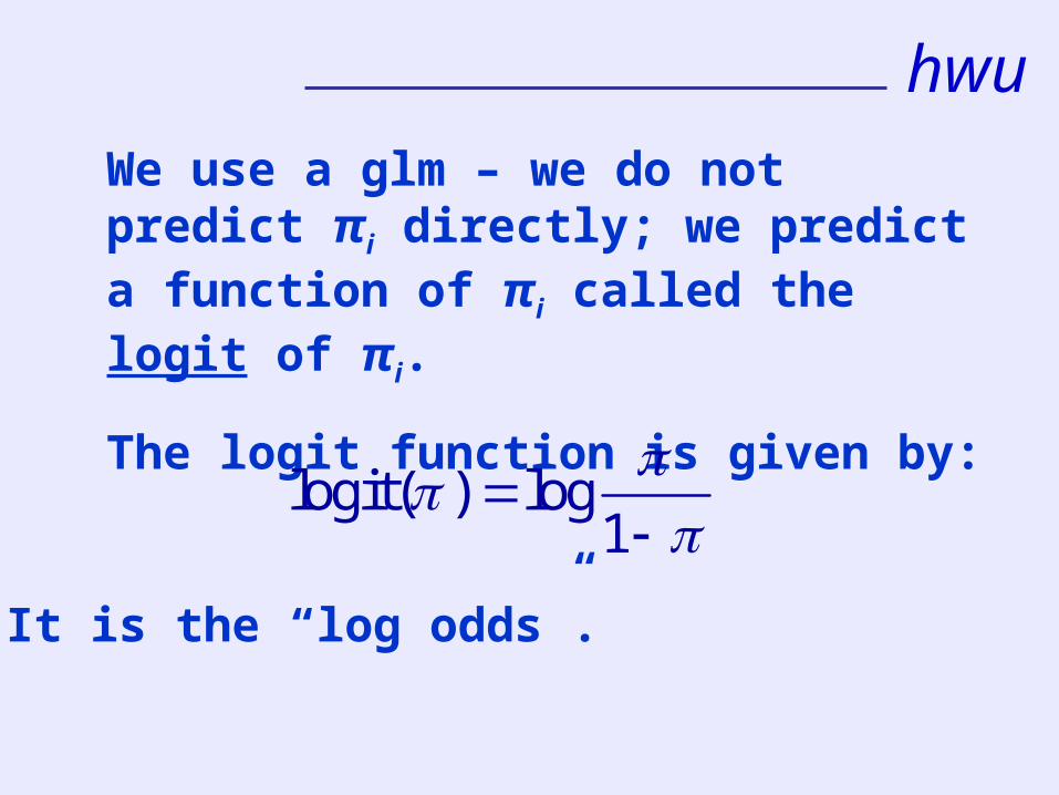
We use a glm – we do not predict πi directly; we predict a function of πi called the logit of πi.
The logit function is given by:
logit( ) log1
It is the “log odds”.

See Illustration 7.1 p 43: proportion v dose
*
*
*
*
*
*
*
*
*
*
3.8 4.0 4.2 4.4 4.6 4.8
0.2
0.4
0.6
0.8
1.0
dose
pro
p

logit(proportion) v dose
*
*
*
*
*
*
*
*
*
3.8 4.0 4.2 4.4 4.6 4.8
-2-1
01
23
dose
log
itpro
p
hwu
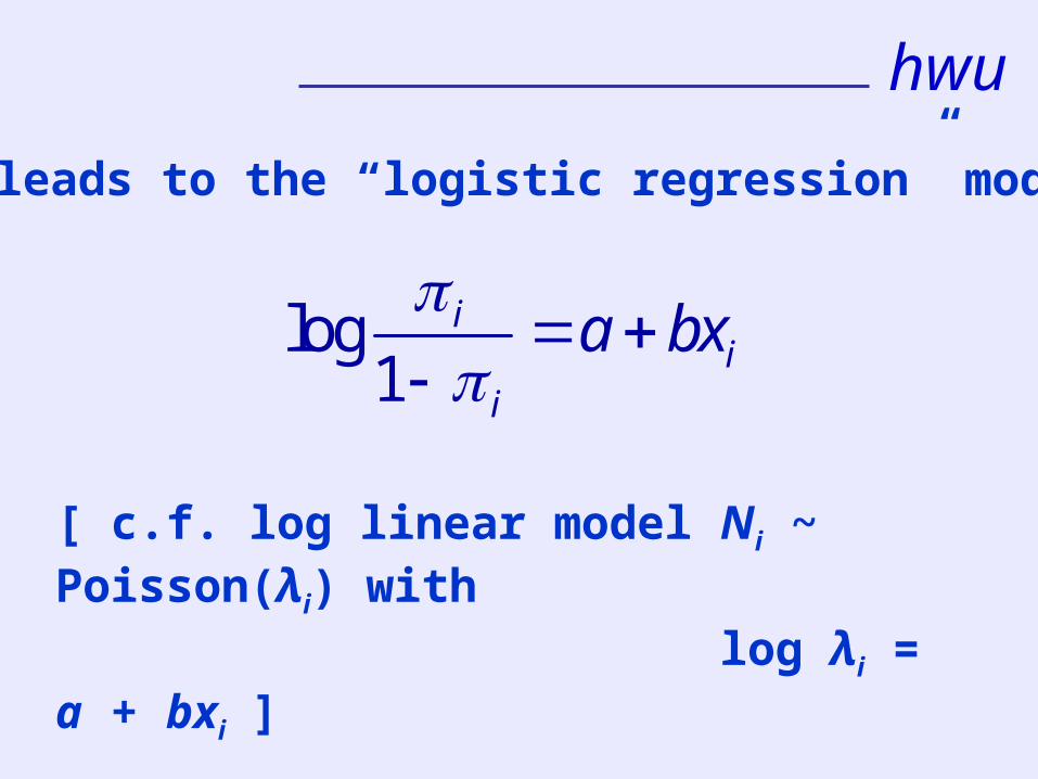
log1
ii
i
a bx
This leads to the “logistic regression” model
[ c.f. log linear model Ni ~ Poisson(λi) with log λi = a + bxi ]

hwu
We are using a logit link
log1
g
We use a linear predictor to explain
rather than itself
log1

hwu
The method based on the use of this model is called logistic regression

hwu
Data: explanatory # successes group observed variable value size proportion
x1 n11 n1 n11/n1
x2 n21 n2 n21/n2
……. xs ns1 ns ns1/ns

hwu
In R we declare the proportion of successes asthe response and include the group sizes as a set of weights
drug.mod1 = glm(propdead ~ dose, weights = groupsize, family = binomial)
explanatory vector is dose note the family declaration

hwu
RHS of model can be extended if required to include additional explanatory variables and factors
e.g. mod3 = glm(mat3 ~ age+socialclass+gender)

hwu
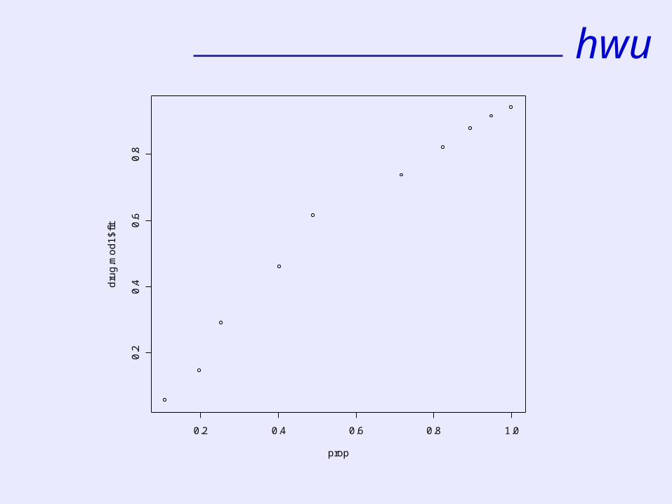
drug.mod – see output p44
Coefficients very highly significant (***) Null deviance 298 on 9df Residual deviance 17.2 on 8df
But … residual v fitted plotand … fitted v observed proportions plot

hwu
-3 -2 -1 0 1 2
-2-1
01
23
Predicted values
Re
sid
ua
ls
glm(formula = num.mat ~ dose, family = binomial)
Residuals vs Fitted
10
5
1
hwu
0.2 0.4 0.6 0.8 1.0
0.2
0.4
0.6
0.8
prop
dru
g.m
od
1$
fit

hwu
0.2 0.4 0.6 0.8 1.0
0.2
0.4
0.6
0.8
1.0
prop
dru
g.m
od
2$
fit
model with aquadraticterm(dose^2)

hwu
8.1 Log-linear models for two-way classifications
Nij ~ Pn(ij) , i= 1,2, …, r ; j = 1,2, …, s
H0: variables are independent
ij = i• •j / ••
§8 MODELS FOR TWO-WAY AND THREE-WAY CLASSIFICATIONS
hwu
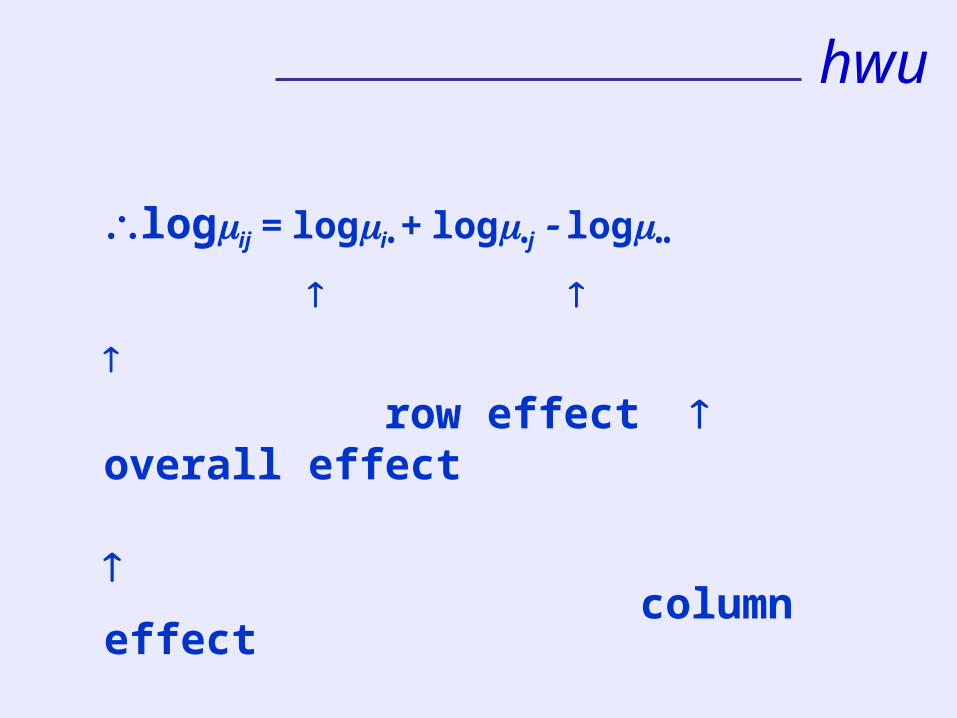
logij = logi• + log•j log••
row effect overall effect column effect

hwu
We “explain” log ij in terms of additive effects: logij = + αi + βj
Fitted values are the expected frequencies
ˆˆˆ ˆexpij i j
Fitting process gives us the value of Y2 = -2logλ

hwu
Nij ~ Pn(ij) , independent, with logij = + αi + βj
Declare the response vector (the cell frequencies) and the row/column codes as factorsthen use > name = glm(…)
Fitting a log-linear model

hwu
Tonsils data (Example 16)
n.tonsils = c(19,497,29,560,24,269)rc = factor(c(1,2,1,2,1,2))cc = factor(c(1,1,2,2,3,3))
tonsils.mod1 = glm(n.tonsils ~ rc + cc, family=poisson)

Call:glm(formula = n.tonsils2 ~ rc + cc, family = poisson)Deviance Residuals: 1 2 3 4 5 6 -1.54915 0.34153 -0.24416 0.05645 2.11018 -0.53736 Coefficients: Estimate Std. Error z value Pr(>|z|) (Intercept) 3.27998 0.12287 26.696 < 2e-16 ***rc2 2.91326 0.12094 24.087 < 2e-16 ***cc2 0.13232 0.06030 2.195 0.0282 * cc3 -0.56593 0.07315 -7.737 1.02e-14 ***---Null deviance: 1487.217 on 5 degrees of freedomResidual deviance: 7.321 on 2 degrees of freedom Y2 = - 2logλ

hwu
The fit of the “independent attributes” model is not good

hwu
> n.patients = c(15, 4, 35, 46)> rc = factor(c(1, 1, 2, 2)) > cc = factor(c(1, 2, 1, 2))
> pat.mod1 = glm(n.patients ~ rc + cc, family = poisson)
Patients data (Example 15)

Call:glm(formula = n.patients ~ rc + cc, family = poisson)Deviance Residuals: 1 2 3 4 1.6440 -2.0199 -0.8850 0.8457 Coefficients: Estimate Std. Error z value Pr(>|z|) (Intercept) 2.251e+00 2.502e-01 8.996 < 2e-16 ***rc2 1.450e+00 2.549e-01 5.689 1.28e-08 ***cc2 2.184e-10 2.000e-01 1.09e-09 1 ---Signif. codes: 0 `***' 0.001 `**' 0.01 `*' 0.05 `.' 0.1 ` ' 1 (Dispersion parameter for poisson family taken to be 1)Null deviance: 49.6661 on 3 degrees of freedomResidual deviance: 8.2812 on 1 degrees of freedom AIC: 33.172

hwu
fitted coefficients: coef(pat.mod1)(Intercept) rc2 cc2 2.251292e+00 1.450010e+00 2.183513e-10
fitted values: fitted(pat.mod1)1 2 3 4 9.5 9.5 40.5 40.5

hwu
1ˆ j
2ˆ j
Estimates are
Predictors for cells 1,1 and 1,2 are 2.251292 :
exp(2.251292) = 9.5
exp(3.701302) = 40.5
Predictors for cells 2,1 and 2,2 are 2.251292 + 1.450010 = 3.701302 :
1 2 1 2ˆˆˆ 2.251292, 0, 1.450010, 0, 0

hwuResidual deviance: 8.2812 on 1 degree of freedom Y2 for testing the model i.e. for testing H0: response is homogeneous/ column distributions are the same/ no association between response and treatment
group
The lower the value of the residual deviance, the better in general is the fit of the model.Here the fit of the additive model is very poor(we have of course already concluded that there is an association – P-value about 1%).

hwu
8.2 Two-way classifications - taking into account a deterministic denominator
See the grouse data (Illustration 8.3 p50, data in Example 25)
Model: Nij ~ Pn(λij) where
E[Nij] = λij = Eij exp( + αi + βj)
logE[Nij/Eij] = + αi + βj
i.e. logλij = logEij + + αi + βj

hwu
We include a term “offset(logE)” in the formulafor the linear predictor
Fitted value is the estimate of the expected response per unit of exposure (i.e. per unit of the offset E)

hwu
8.3 Log-linear models for three-way classifications
Each subject classified according to 3factors/variables with r,s,t levels respecitvely
Nijk ~ Pn(ijk) withlog ijk = + αi + βj + γk + (αβ)ij + (αγ)ik + (βγ)jk + (αβγ)ijk
r s t parameters

hwu
Model with two factors and an
interaction (no longer additive) is
log ij = + αi + βj + (αβ)ij
Recall “interaction”

hwu
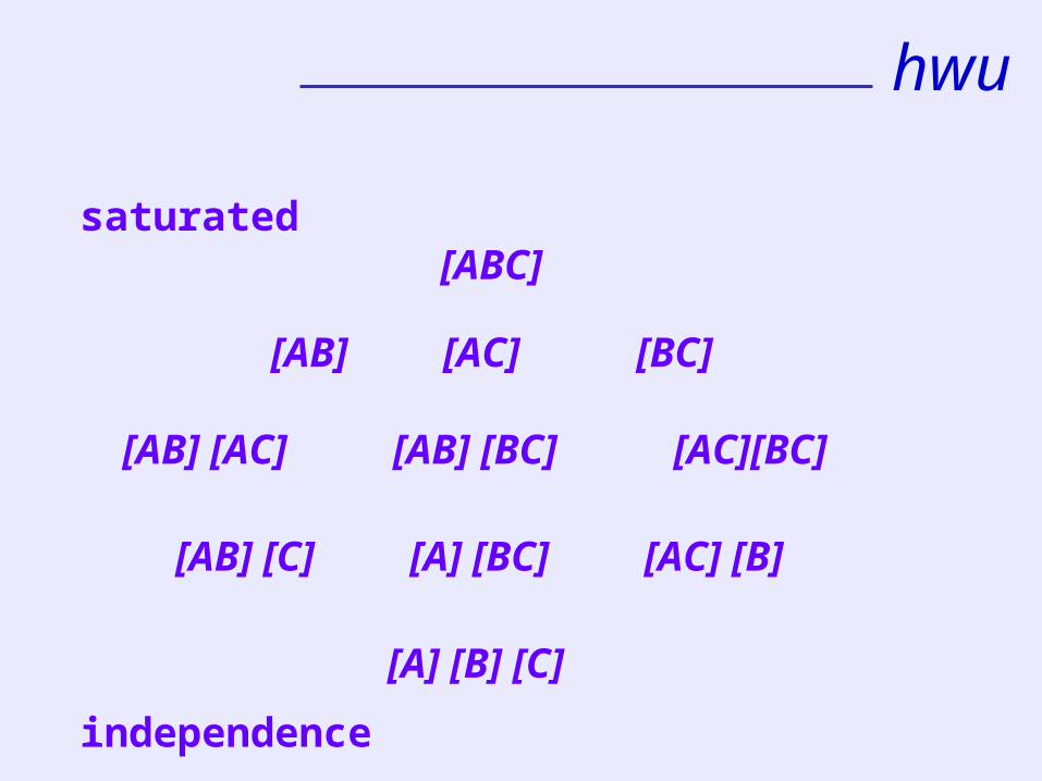
Range of possible models/dependenciesFrom1 Complete independence
model formula: A + B + C
link: log ijk = + αi + βj + γk
notation: [A][B][C]df: rst – r – s – t + 2
8.4 Hierarchic log-linear models
Interpretation!

hwu
…. through
2 One interaction (B and C say)model formula: A + B*C link: log ijk = + αi + βj + γk + (βγ)jk
notation: [A][BC]
df: rst – r – st + 1

hwu
…. to
5 All possible interactionsmodel formula: A*B*C
notation: [ABC]
df: 0

hwu
Model selection: by
backward elimination or forward selection
through the hierarchy of modelscontaining all 3 variables
hwu
saturated [ABC]
[AB] [AC] [BC]
[AB] [AC] [AB] [BC] [AC][BC]
[AB] [C] [A] [BC] [AC] [B]
[A] [B] [C] independence

hwu
Our models can include
mean (intercept)
+ factor effects
+ 2-way interactions
+ 3-way interaction
hwu
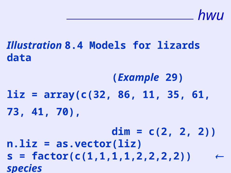
Illustration 8.4 Models for lizards data (Example 29)
liz = array(c(32, 86, 11, 35, 61, 73, 41, 70), dim = c(2, 2, 2))n.liz = as.vector(liz)s = factor(c(1,1,1,1,2,2,2,2)) species d = factor(c(1, 1, 2, 2, 1, 1, 2, 2)) diameter of perchh = factor(c(1,2,1,2,1,2,1,2)) height of perch

hwu
Forward selectionliz.mod1 = glm(n.liz ~ s + d + h, family = poisson) liz.mod2 = glm(n.liz ~ s*d + h, family = poisson) liz.mod3 = glm(n.liz ~ s + d*h, family = poisson)liz.mod4 = glm(n.liz ~ s*h + d, family = poisson)liz.mod5 = glm(n.liz ~ s*d + s*h, family = poisson)liz.mod6 = glm(n.liz ~ s*d + d*h, family = poisson)
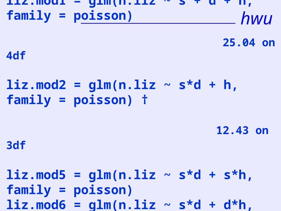
hwuForward selectionliz.mod1 = glm(n.liz ~ s + d + h, family = poisson) 25.04 on 4df
liz.mod2 = glm(n.liz ~ s*d + h, family = poisson) † 12.43 on 3df
liz.mod5 = glm(n.liz ~ s*d + s*h, family = poisson)liz.mod6 = glm(n.liz ~ s*d + d*h, family = poisson)

hwu
Forward selectionliz.mod1 = glm(n.liz ~ s + d + h, family = poisson)
liz.mod2 = glm(n.liz ~ s*d + h, family = poisson) †
liz.mod5 = glm(n.liz ~ s*d + s*h, family = poisson)† 2.03 on 2df

hwu> summary(liz.mod5)Call:glm(formula = n.liz ~ s * d + s * h, family = poisson)Coefficients: Estimate Std. Error z value Pr(>|z|) (Intercept) 3.4320 0.1601 21.436 < 2e-16 ***s2 0.5895 0.1970 2.992 0.002769 ** d2 -0.9420 0.1738 -5.420 5.97e-08 ***h2 1.0346 0.1775 5.827 5.63e-09 ***s2:d2 0.7537 0.2161 3.488 0.000486 ***s2:h2 -0.6967 0.2198 -3.170 0.001526 ** Null deviance: 98.5830 on 7 degrees of freedomResidual deviance: 2.0256 on 2 degrees of freedom

hwu
*
*
*
*
*
*
*
*
20 40 60 80
20
40
60
80
n.liz
liz.m
od
5$
fit

hwu
*
*
*
*
*
*
*
*
20 40 60 80
-0.1
0-0
.05
0.0
00
.05
0.1
0
liz.mod5$fit
liz.m
od
5$
res

hwu
FIN

hwu
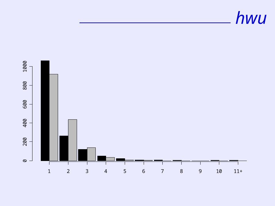
Number of papers per author 1 2 3 4 5 6 7 8 9 10 11Number of authors 1062 263 120 50 22 7 6 2 0 1 1
MAJOR ILLUSTRATION 1
, 1, 2, 3,...!
x
P X x xx
Model

hwu
0.90 0.92 0.94 0.96 0.98 1.00
4.5
5.0
5.5
th
log
l2
hwu
1 2 3 4 5 6 7 8 9 10 11+
02
00
40
06
00
80
01
00
0

hwu

hwu
MAJOR ILLUSTRATION 2
Hedge type i A B C D E F GHedge length (m) li 2320 2460 2455 2805 2335 2645 2099Number of pairs ni 14 16 14 26 15 40 71
Model Ni ~ Pn(ili)

hwu
1 2 3 4 5 6 7
01
02
03
04
05
0
type
de
nsi
ty
x xx
x
x
x
x
x x x
x
x
x
x

hwuCyclic models
DNOSAJJMAMFJ
60
50
40
30
Month
case
s
leukaemia data

hwu
Model
Ni independent Pn(λi) with
0
0
exp cos
exp cos sin , 1, ...,
exp cos sin
i i
i i
i i
a b i r
c a b
Explanatory variable: the category/month i has been transformed into an angle i

hwu
It is another example of a non-linear regression model for Poisson responses.
It is a generalised linear model.

hwu
Fitting in R>n=c(40, 34, …, 33, 38) response vector>r=length(n)>i=1:r>th=2*pi*i/r explanatory vector
model>leuk=glm(n~cos(th) + sin(th),family=poisson)

hwu
ˆ exp 3.73069 0.17177cos 0.11982sini i i
Fitted mean is

hwu
J F M A M J J A S O N D
30
40
50
60
Month
case
s
cyclic model for leukaemia data
Fitted model

hwu
Male Female
Cinema often 22 21
Not often 20 12
F73DB3 CDA Data from class

hwu
Male Female
Cinema often 22 21 43
Not often 20 12 32
42 33 75

Male Female
Cinema often 22 21 43
Not often 20 12 32
42 33 75
P(often|male) = 22/42 = 0.524P(often|female) = 21/33 = 0.636significant difference (on these numbers)?is there an association between gender and cinema attendance?
hwu
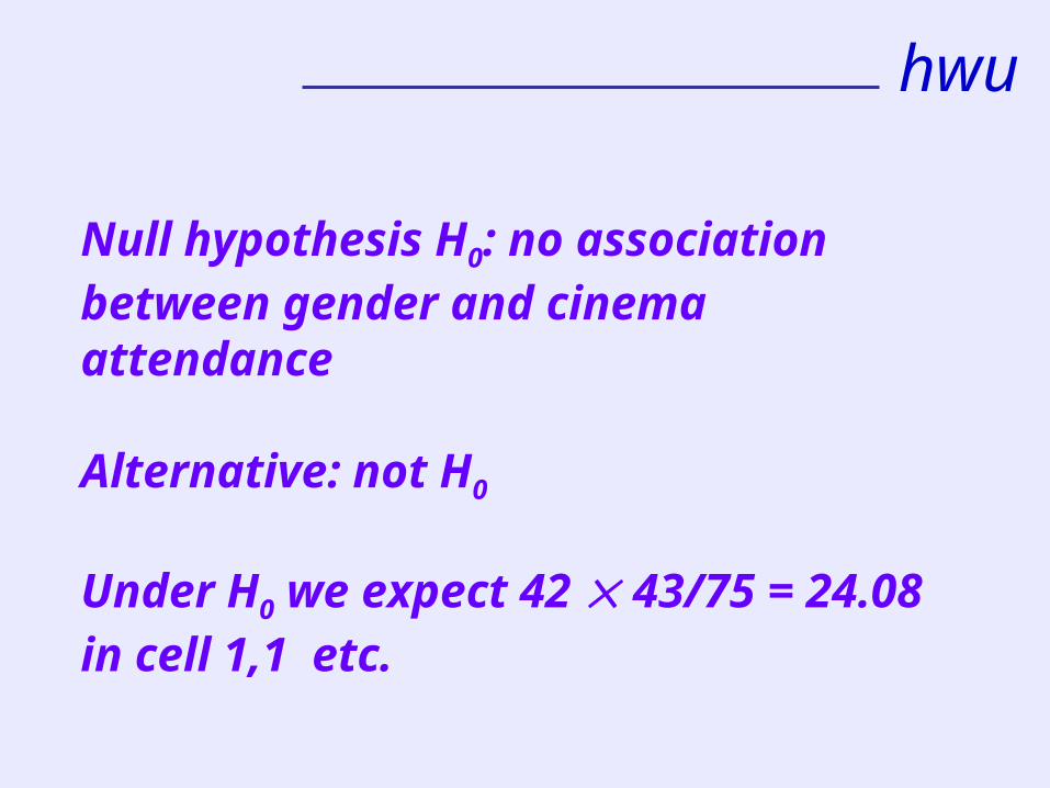
Null hypothesis H0: no association between gender and cinema attendance
Alternative: not H0
Under H0 we expect 42 43/75 = 24.08 in cell 1,1 etc.
hwu
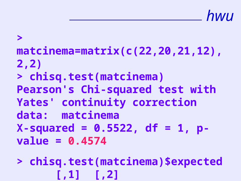
> matcinema=matrix(c(22,20,21,12),2,2)> chisq.test(matcinema)Pearson's Chi-squared test with Yates' continuity correctiondata: matcinema X-squared = 0.5522, df = 1, p-value = 0.4574
> chisq.test(matcinema)$expected [,1] [,2][1,] 24.08 18.92 [2,] 17.92 14.08
hwu
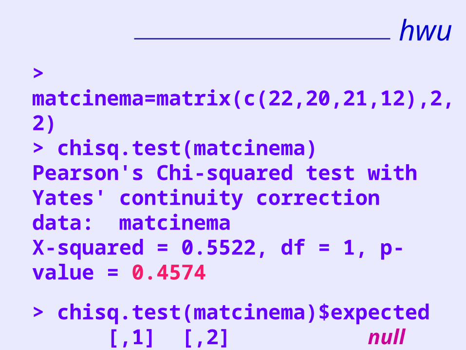
> matcinema=matrix(c(22,20,21,12),2,2)> chisq.test(matcinema)Pearson's Chi-squared test with Yates' continuity correctiondata: matcinema X-squared = 0.5522, df = 1, p-value = 0.4574
> chisq.test(matcinema)$expected [,1] [,2] null hypothesis can stand [1,] 24.08 18.92 no association between gender[2,] 17.92 14.08 and cinema attendance

hwu
Male Female
Cinema often 110 105 215
Not often 100 60 160
210 165
P(often|male) = 110/210 = 0.524P(often|female) = 105/60 = 0.636significant difference (on these numbers)?
more students, same proportions

hwu
> matcinema2=matrix(c(110,100,105,60),2,2)> chisq.test(matcinema2)Pearson's Chi-squared test with Yates' continuity correctiondata: matcinema2

hwu
> matcinema2=matrix(c(110,100,105,60),2,2)> chisq.test(matcinema2)Pearson's Chi-squared test with Yates' continuity correctiondata: matcinema2 X-squared = 4.3361, df = 1, p-value = 0.03731> chisq.test(matcinema2)$expected [,1] [,2][1,] 120.4 94.6[2,] 89.6 70.4

hwu
> matcinema2=matrix(c(110,100,105,60),2,2)> chisq.test(matcinema2)Pearson's Chi-squared test with Yates' continuity correctiondata: matcinema2 X-squared = 4.3361, df = 1, p-value = 0.03731> chisq.test(matcinema2)$expected
[,1] [,2] null hypothesis is rejected[1,] 120.4 94.6 there IS an association between[2,] 89.6 70.4 gender and cinema attendance

hwu
FIN