f soft response generation and thresholding strategies for...

Soft Response Generation and Thresholding Strategies for Linear and Feed-Forward MUX PUFs

Chen Zhou, Saroj Satapathy, Yingjie Lao, Keshab K. Parhi and Chris H. Kim Department of ECE, University of Minnesota, Minneapolis, MN

{zhoux825, sata0002, laoxx025, parhi, chriskim}@umn.edu

ABSTRACT

In this work, we present probability based response generation schemes for MUX based Physical Unclonable Functions (PUFs). Compared to previous implementations where temporal majority voting (TMV) based on limited samples and coarse criteria was utilized to determine final responses, our design can collect soft

responses with detailed probability information using simple on-chip circuits. Thresholds with fine accuracy are applied to efficiently distinguish stable and unstable challenge response pairs (CRPs). A 32nm test chip including both linear and feed-forward MUX PUFs was implemented for concept verification. Based on a detailed analysis of the hardware data, we propose several enhanced thresholding strategies for determining stable CRPs. For instance, a stringent threshold can be imposed in enrollment phase

for selecting good CRPs, while a relaxed threshold can be used during normal authentication phase. Experimental data shows a high degree of uniqueness and randomness in the PUF responses which can be attributed to the carefully optimized circuit layout. Finally, output characteristic of a feed-forward MUX PUF was compared to that of a standard linear MUX PUF from the same 32nm chip.

CCS Concepts

•Hardware➝Application specific integrated circuits •Security

and privacy➝Hardware security implementation.

Keywords

Physical unclonable function; MUX based PUF; soft response; thresholding; massive statistics; feed-forward.

1. INTRODUCTION Physical unclonable function or PUF has been widely accepted as

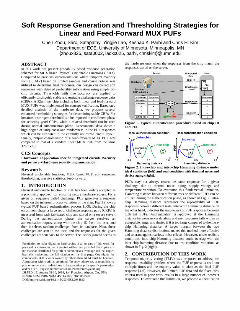
a promising approach for ensuring secure hardware access. For a given bit sequence called challenge, PUF generates a response based on the inherent process variation of the chip. Fig. 1 shows a typical PUF based authentication process [1-3]. During the chip enrollment phase, a large set of challenge response pairs (CRPs) is measured from each fabricated chip and stored on a secure server. During the authentication phase, the server receives an authentication request along with the chip ID from the user, and then it selects random challenges from its database. Next, these

challenges are sent to the user, and the responses for the given challenges are sent back to the server. The user is granted access to

the hardware only when the responses from the chip match the

responses stored on the server.

Approve Deny

Chip ID

Retrieve

CRP subset

Encrypted

Data

Database

Chip

PUF

ID

Challenge

209A (Hex)

41B1 (Hex)

9283 (Hex)

Response

0

1

1

Server User

Compare

Response

0

1

1

Challenges

Responses

Decision

Figure 1. Typical authentication procedure based on chip ID

and PUF.

Hamming distance

PD

F

0.5

Intra-chip

Inter-chip

1.00.0

Ideal authentication condition

margin>0

Hamming distance0.5

Intra-chip

Inter-chip

1.00.0

margin<0

Real authentication condition

PD

F

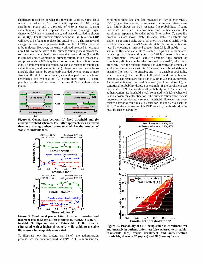
Figure 2. Intra-chip and inter-chip Hamming distance under

ideal condition (left) and real condition with thermal noise and

device aging (right).

PUFs may not always return the same response for a given challenge due to thermal noise, aging, supply voltage and temperature variation. To overcome this fundamental limitation,

Hamming distance between different tests or different PUFs can be utilized during the authentication phase, as shown in Fig. 2. Intra-chip Hamming distance represents the repeatability of PUF responses between different tests. Inter-chip Hamming distance on the other hand, indicates the uniqueness of PUF responses between different PUFs. Authentication is approved if the Hamming distance between server database and user responses falls within an acceptable range, and denied if it is too large compared to the intra-

chip Hamming distance. A larger margin between the two Hamming distance distributions makes this method more effective and tolerant against various noise effects. However, under realistic conditions, intra-chip Hamming distance could overlap with the inter-chip hamming distance due to test condition variation, as shown in Fig. 2 (right).

2. CONTRIBUTION OF THIS WORK Temporal majority voting (TMV) was proposed to address the response instability problem where the PUF response is read out multiple times and the majority value is taken as the final PUF response [4-6]. However, the limited PUF data and the fixed 50% criteria used in prior work results in a large number of incorrect responses. To overcome this limitation, we propose authentication

Permission to make digital or hard copies of all or part of this work for

personal or classroom use is granted without fee provided that copies are

not made or distributed for profit or commercial advantage and that copies

bear this notice and the full citation on the first page. Copyrights for

components of this work owned by others than ACM must be honored.

Abstracting with credit is permitted. To copy otherwise, or republish, to

post on servers or to redistribute to lists, requires prior specific permission

and/or a fee. Request permissions from [email protected].

ISLPED '16, August 08-10, 2016, San Francisco Airport, CA, USA

© 2016 ACM. ISBN 978-1-4503-4185-1/16/08$15.00 DOI: http://dx.doi.org/10.1145/2934583.2934613

strategies based on soft responses and improved thresholding. A soft response is defined as the probability of a response being ‘1’ for a given challenge. Its value is derived from 100K repetitive PUF measurements for each challenge using fast on-chip sampling circuits. For instance, if the response output is ‘1’ for 99K out of

100K measurements, the corresponding soft response value is 0.99. Compared with the previous TMV scheme, our results based on a massive number of samples provide more insight into the detailed PUF operation. To generate the binary response from the soft response, we apply probability thresholds to classify the response bits into one of three categories: stable ‘0’, stable ‘1’ or unstable. Adjustable thresholds are used in our work which is different from previous TMV schemes. Our experimental results show that by

selecting the stable CRPs based on soft responses, the PUFs can work reliably under a wider range of VDD and temperature. Vulnerability to modelling attacks is a weakness of standard MUX based PUFs. To overcome this concern, a feed-forward path structure was proposed in [7]. We present data for both linear MUX PUF and feed-forward MUX PUF fabricated in the same 32nm test chip.

3. SOFT RESPONSE COLLECTION

CIRCUITS

c1

On-

chip

VCO

c2 c32

32 MUX stages Arbiter

On-chip

counterSR

Latch

S Q

ROn-chip

counter

M

Response

N

Pr(Response='0') = — M

N

>1GHz

1

PUF stage

(c='1')

0

PUF stage

(c='0')

SR latch

arbiter

S

R

Q

S R Q

0 0 1

0 1 1

1 0 0

1 1 Q

Response = '0'

'0'

S

R

Reset Test

Q

S

R

'1'Q

Response = '1'

Reset Test

Pr(Response='1') = 1- — M

N

Δ

Soft response

Figure 3. Proposed MUX based PUF design utilizing an on-chip

voltage controlled oscillator circuit and counters to efficiently

collect soft response.

The traditional PUF evaluation process is as follows: 1) challenge bits 𝑐1~𝑐32 are applied; 2) a rising edge is fed to two paths

simultaneously; 3) the SR latch based arbiter generates a response bit output based on the delay difference. Fig. 3 shows the proposed PUF design which can collect massive PUF data using an on-chip voltage controlled oscillator running at gigahertz frequencies. The basic idea is to measure the probability of the response being ‘1’ or

‘0’ using an on-chip counter which counts the arbiter outputs, and compare the value with the total number of VCO cycles. The ratio between the two count values is the probability of the response being ‘0’. The probability of response being ‘1’, denoted as 𝑃𝑟(𝑅𝑒𝑠𝑝𝑜𝑛𝑠𝑒 = ′1′) , is also available based on the equation:

𝑃𝑟(𝑅𝑒𝑠𝑝𝑜𝑛𝑠𝑒 = ′1′) = 1 − 𝑃𝑟(𝑅𝑒𝑠𝑝𝑜𝑛𝑠𝑒 = ′0′) . Unlike the

traditional response which can only be ‘1’ or ‘0’, 𝑃𝑟(𝑅𝑒𝑠𝑝𝑜𝑛𝑠𝑒 =′1′) could vary from 0% to 100%, and is defined as soft response.

Fig. 4 shows how soft response is affected by the process corner. Challenges that induce strong positive bias or strong negative bias in the final delay difference produces less instability, resulting in soft response close to 0% or 100%. Challenges that create a weak delay difference bias lead to soft response between 0% and 100%.

These CRPs are responsible for PUF intra-die variation. Using soft response and comparing it with a threshold, we can classify CRPs

into three categories: stable ‘0’, stable ‘1’, and unstable. Only stable bits will be used by the server for authentication application. The advantage of this strategy is explained in further detail in following section.

Δ

PDFµ: process

variation σ:

noise

(a)

Soft response

= 0.0

Strong negative

bias

Δ

PDF

(b)

Soft response

= 0.3

Weak negative

bias

Δ

PDF

(c)

Soft response

= 0.7

Δ

PDF

(d)

Soft response

= 1.0

Strong positive

bias

Δ: Delay different

of final stage

Weak positive

bias

Figure 4. Output statistics reveal process variation under given

challenge. Soft response behaviors for challenges inducing (a)

strong negative, (b) weak negative, (c) weak positive and (d)

strong positive biases.

4. PUF MEASUREMENT RESULTS This section shows that various aspects of the linear MUX arbiter PUF fabricated in 32nm including soft response characteristics, reliability, uniqueness, Hamming distance margin, flexible threshold strategies, and randomness.

4.1 Soft response characteristics

Soft response

Pro

ba

bilit

y (

%)

10

20

30

40

50

60

70

80

90

100

0

1 PUF, 0.9V, 25ºC

33,000 challenge-response pairs

x 100K VCO cycles

= 3.15 Gb responses total

0 0.2 0.4 10.80.6

Pr(stable '0') = 48.24 %

Pr(stable '1') = 45.92 %

Pr(unstable) = 5.84 %

Threshold for '0'

= 1-Threshold for '1'

= 0.2

Threshold

for '1' = 0.8

Stable '0' Stable '1'Unstable

Soft response0 0.2 0.4 0.6 0.8 1

10

10

10

10

10

-2

-1

0

1

2

Pro

ba

bilit

y (

%)

Figure 5. Measured soft response (i.e. probability of response

being ‘1’) distribution of standard MUX PUF in linear (upper

figure) and semi-log (lower figure) scales. The threshold used

for defining unstable and stable responses can be adjusted

based on the reliability and security requirements.

Fig. 5 shows the soft response distribution for a single PUF in both linear and log scale. 33,000 CRPs are tested and each CRP is tested repeatedly 100K times using the on-chip sampling circuits. The CRPs are labeled as stable ‘0’ or stable ‘1’or unstable, based on the soft response. For example, in Fig. 5, 0.8 is chosen as the threshold

for stable ‘1’. For simplicity, the symmetric value of 0.2 is chosen as the threshold for stable ‘0’. Under these conditions, the percentages of stable ‘1’, stable ‘0’, and unstable bits are 45.92%, 48.24% and 5.84%, respectively. The combined probability of stable ‘0’ and ‘1’ bits is 94.16%, meaning that the majority of challenges lead to relatively stable responses.

4.2 PUF reliability and uniqueness versus

threshold

The method we used for calculating Hamming distance in the presence of unstable responses is given in Fig. 6. CRPs with

unstable response are discarded. Then additional CRPs are utilized to replace the discard ones to ensure the comparison length is constant for all tests. This method works for both intra-chip and inter-chip Hamming distance calculation. Ideally, the intra-chip Hamming distance is zero, and the inter-chip Hamming distance distribution on a large set of PUFs has a mean value of 0.5.

Fig. 7 shows the Hamming distance distributions for different threshold values. Test conditions were varied as follows: 0.8~1.0V

for VDD and 25~85ºC for temperature. Three different threshold values were considered for stable ‘1’: 0.50, 0.85 and 1.00. Symmetric values were used for the stable ‘0’ threshold to simplify the analysis. The inter-chip Hamming distance distribution is close to ideal and hardly changed, suggesting a symmetric layout design and weak correlation between threshold value and uniqueness.

Response

sequence #1

Response

sequence #2

0 1 0 1 0 0 1

0 0 1 1 1 0 1

Replace discarded

CRPs with new onesInitial N CRPs

Bit errorUnstable CRP:

discarded

Hamming distance = # of bit error

N

Hamming distance calculation for N CRPs

1

1

Figure 6. Hamming distance calculation utilizing only the

stable CRPs.

When the threshold is set to 0.5, no CRP is considered to be unstable. As shown in the Fig. 7 (top), the margin between intra-chip and inter-chip Hamming distance distributions is negative 0.0625, meaning that the two distributions overlap. Please note that the traditional one time sampling method will result in an overlap even larger than Fig. 7 (top) because of the small sample size. Fig.

7 (middle) shows results when the threshold is 0.85. Only responses with a probability value greater than 0.85 or less than 0.15 are used for authentication purposes. As a result, the average and sigma values of intra-chip Hamming distance are both 14% of those when threshold is 0.5. The distribution margin increases to positive 0.0157. Furthermore, when the threshold value is set to 1, meaning only absolute stable responses are accepted, the intra-chip Hamming distance average and sigma values are only 0.16% and

0.084% of those when threshold is 0.5, respectively. Therefore, the distribution margin is now positive 0.0625, which guarantees the success of authentication. Table 1 shows the margin between the two distributions as well as the percentage of stable ‘0’ and ‘1’ bits for different thresholds. A threshold greater than 0.85 will result in

no overlap between the two distributions and more than 81.15% of the responses being stable ‘0’ or stable ‘1’. During enrollment phase, each PUF is tested under a nominal VDD and temperature condition. Only the CRPs with a soft response value greater than 0.85 (or less than 0.15) are stored on the server and utilized for

future authentication purposes. Since those stable CRPs will have a lower probability of becoming the opposite stable value, we can generate more reliable PUF responses in the presence of PVT variation and aging.

VDD: 0.8~1.0V (normal: 0.9V) 32nm Temp.: 25~85ºC

Hamming Distance (normalized) Hamming Distance (normalized)0 0.2 0.4 0.6 0.8 10 0.2 0.4 0.6 0.8 1

Pro

ba

bil

ity (

%)

Pro

ba

bil

ity (

%)

0

20

40

60

80

100

10

10

10

10

10

10

-3

-2

-1

0

1

2

Threshold for '0' and '1' = 0.50

Intra-chip

µ = 3.71e-2

Maximum=0.1719

σ = 1.08e-3 µ = 0.488 σ = 0.0918

Minimum=0.1094

Inter-chip

(576 PUFs)

Margin =

- 0.0625 (overlap)


Pro

ba

bil

ity (

%)

Pro

ba

bil

ity (

%)

0

20

40

60

80

100

10

10

10

10

10

10

-3

-2

-1

0

1

2

Intra-chip

µ = 5.30e-3

Maximum=0.0781

σ = 1.53e-4 µ = 0.487 σ = 0.0991

Minimum=0.0938

Inter-chip

(576 PUFs)

Margin =

0.0157

Threshold for '0' = 0.15



Pro

ba

bil

ity (

%)

Pro

ba

bil

ity (

%)

0

20

40

60

80

100

10

10

10

10

10

10

-3

-2

-1

0

1

2

Intra-chip

µ = 5.79e-5

Maximum=0.0156

σ = 9.03e-7 µ = 0.487 σ = 0.114

Minimum=0.0781

Inter-chip

(576 PUFs)

Margin =

0.0625



64 stable CRPs

100K VCO cycles for each evaluationIntra-chip: 4 PUFs from 2 chips

Inter-chip: 576 PUFs from 6 chips

Figure 7. Intra-chip and inter-chip Hamming distance

distributions in linear scale (left column) and semi-log scale

(right column), under different threshold values.

Table 1. Stable CRPs selection and intra/inter-chip Hamming

distance distribution gap versus threshold (0.8~1.0V, 25~85ºC) Threshold for

‘1’/‘0’

In 10,000 random CRPs Margin between

distributions (norm.,

64 CRPs) % of stable

‘0’

% of stable

‘1’

0.50 / 0.50 51.18% 48.85% -0.0625 (overlap)

0.55 / 0.45 50.74% 48.42% -0.0469 (overlap)

0.60 / 0.40 50.31% 48.00% -0.0469 (overlap)

0.65 / 0.35 49.80% 47.56% -0.0313 (overlap)

0.70 / 0.30 49.36% 47.03% -0.0469 (overlap)

0.75 / 0.25 48.83% 46.52% -0.0469 (overlap)

0.80 / 0.20 48.24% 45.92% -0.0313 (overlap)

0.85 / 0.15 47.55% 45.30% 0.0157 (no overlap)

0.90 / 0.10 46.61% 44.45% 0.0313 (no overlap)

0.95 / 0.05 45.32% 43.15% 0.0625 (no overlap)

1.00 / 0.00 41.50% 39.65% 0.0625 (no overlap)

4.3 Enhanced thresholding strategies In the previous section, we have shown that PUF responses can be made more reliable by utilizing a soft response. It is worth noting though that some stable challenges may inevitably become unstable

challenges regardless of what the threshold value is. Consider a scenario in which a CRP has a soft response of 0.81 during enrollment phase and a threshold of 0.80 is chosen. During authentication, the soft response for the same challenge might change to 0.79 due to thermal noise, and hence discarded as shown

in Fig. 8(a). For the authentication scheme in Fig. 6, a new CRP will have to be found to replace this unstable CRP. The latency and energy overhead are proportional to the number of CRPs that need to be replaced. However, the extra workload involved in testing a new CRP could be saved if the authentication process allows the soft response to marginally cross over the threshold line (i.e., 0.79 is still considered as stable in authentication). It is a reasonable compromise since 0.79 is quite close to the original soft response

0.81. To implement this tolerance, we can use relaxed thresholds in authentication, as shown in Fig. 8(b). Please note that the stable-to-unstable flips cannot be completely avoided by employing a more stringent threshold. For instance, even if a particular challenge generates a soft response of 1.0 in enrollment phase, it is still possible for the soft response to become 0.99 in authentication phase.

0 1.0Soft response

0 1

Due to noise

0 1.0Soft response

0 1

(a) (b)

Due to noise

unstable unstable

Relaxed threshold

Enroll.

Auth.

0.81 0.81

0.79Fixed threshold

0.79

Figure 8. Comparison between (a) fixed threshold and (b)

relaxed threshold schemes. The latter approach uses a relaxed

threshold during authentication to minimize the number of

stable-to-unstable flips.

95

100

0

5

Enroll.: stable'1'

Pro

ba

bil

ity (

%) Pr(Auth.: stable'1' | Enroll.: stable'1')

Pr(Auth.: unstable | Enroll.: stable'1')

Pr(Auth.: stable'0' | Enroll.: stable'1')

Threshold for '1'

Enrollment: 0.9V, 25ºC

Authentication: 1.0V, 85ºC100K VCO cycles

0.5 0.6 0.7 0.8 0.9 1.0

1 PUF, 1000 CRPs

Threshold for '1'

Pro

ba

bil

ity (

%)


Pr(Auth.: unstable | Enroll.: stable'0')


Enrollment: 0.9V, 25ºC

Authentication: 1.0V, 85ºC

0.5 0.6 0.7 0.8 0.9 1.0

Enroll.: stable'0'

95

100

0

5

100K VCO cycles

1 PUF, 1000 CRPs

Figure 9. Conditional probabilities of correct, unstable, and

incorrect responses for different threshold values. Stable ‘1’-

to-stable ‘0’ flips and stable ‘0’-to-stable ‘1’ flips can be

eliminated with a higher threshold, while stable-to-unstable

flips cannot be completely eliminated.

To illustrate how this strategy can benefit the authentication process, we use data measured at 0.9V, 25ºC to represent the

enrollment phase data, and data measured at 1.0V (higher VDD), 85ºC (higher temperature) to represent the authentication phase data. Fig. 9 shows the PUF response flip probabilities if same thresholds are used in enrollment and authentication. For enrollment response to be either stable ‘1’ or stable ‘0’, three flip

probabilities are shown: stable-to-stable, stable-to-unstable and stable-to-opposite-stable. Out of all the CRPs deemed stable by the enrollment test, more than 93% are still stable during authentication test. By choosing a threshold greater than 0.82, all stable ‘1’-to-stable ‘0’ flips and stable ‘0’-to-stable ‘1’ flips can be eliminated, indicating that a threshold larger than 0.82 is a reasonable choice for enrollment. However, stable-to-unstable flips cannot be completely eliminated unless the threshold is set to 0.5, which isn’t

practical. Then the relaxed threshold in authentication strategy is applied on the same data set. Fig. 10 shows the combined stable-to-unstable flip (both ‘0’-to-unstable and ‘1’-to-unstable) probability when sweeping the enrollment threshold and authentication threshold. The results are plotted in Fig. 10, in 3D and 2D formats. As the authentication threshold is relaxed (i.e., lowered for ‘1’), the conditional probability drops. For example, if the enrollment test threshold is 0.9, the conditional probability is 0.9% when the

authentication test threshold is 0.7, compared with 3.7% when 0.9 is still chosen for authentication. The authentication efficiency is improved by employing a relaxed threshold. However, an over-relaxed threshold could make it easier for the attacker to hack the PUF. Therefore, to ensure high PUF security, the threshold value must be chosen carefully.

0.90.8

0.70.6

0.51.00.9

0.80.7

0.60.50

2

6

8

4

0 1 2 3 4 5 6

1.0

Pr(

Au

th.:

un

sta

ble

| E

nro

ll.:

sta

ble

) (%

)

Enrollment test: 0.9V, 25ºC

Authentication test: 1.0V, 85ºC

0.5 0.6 0.7 0.8 0.90.5

0.6

0.7

0.8

0.9

1.0

1.0Enrollment threshold for '1'

Au

then

tic

ati

on

th

resh

old

fo

r '1

'

Pr(Auth.: unstable |

Enroll.: stable) (%)

[0, 1.0](1.0, 2.0]

(3.0, 4.0]

>4.0

Figure 10. Probability of CRP being stable in enrollment test

and unstable in authentication test (also referred to as stable-

to-unstable flips) versus enrollment and authentication

thresholds, shown in 3D (upper) and 2D (bottom) format.

4.4 PUF randomness Randomness is another important metric for PUFs since a random

PUF response is harder to predict. Strong biases should not be exhibited in the responses under randomly chosen challenges as this info can be used by the attacker to predict the responses, rendering the PUF ineffective. The number of ‘1’s (or ‘0’s) for randomly chosen responses is usually counted to check a PUF’s randomness. Ideally, the percentage of ‘1’s or ‘0’s should be close to 50%, since this will allow the maximum number response

combinations, i.e., ( 𝑛𝑛/2

) =𝑛!

𝑛2⁄ !𝑛 2⁄ !

, where 𝑛 is the total number of

CRPs. This makes it more difficult for the attacker to predict the correct response value. However, in the presence of process variation, randomness of a PUF usually follows a normal distribution. Fig. 11 shows the randomness distribution of 576 PUFs measured from 6 chips. Unstable responses that fall outside of the stable zone were discarded. We did not observe any obvious chip to chip variation in the randomness data.

32nm, 0.9V, 25ºC

Pr(stable '1')

Pro

ba

bil

ity (

%)

0 0.2 0.4 0.8 10.60

1

2

3

4

5

6576 PUFs from 6 chips

64 stable CRPs

Thr('1') = 0.8

Thr('0') = 0.2

µ = 0.563

σ = 0.132

Figure 11. Measured randomness of MUX PUF

5. COMPARISON OF LINEAR AND FEED-

FORWARD MUX PUF

This section introduces the feed-forward PUF that was also implemented in the same chip, along with modeling attack results on both the linear PUF and feed-forward PUF. We also compare the stability of the two PUF designs.

5.1 Linear PUF Modeling attacks

PUFs are expected to be resistant against modelling attacks. However, it has been shown that a machine learning based approach can predict all CRPs with a high success rate using a subset of the CRPs as training data. Linear MUX PUF is particularly vulnerable to modelling attacks due to the linear relationship between the input challenge and output response. We employ an additive linear delay model [8, 9] for testing modelling attack on our linear MUX PUF.

𝐶 =

[ (2𝑐1 − 1)(2𝑐2 − 1)⋯ (2𝑐32 − 1)

(2𝑐2 − 1)⋯ (2𝑐32 − 1) ⋮ (2𝑐32 − 1) 1]

𝑇

𝑊 =1

2

[

𝛿10 − 𝛿1

1

𝛿10 + 𝛿1

1 + 𝛿20 − 𝛿2

1

⋮𝛿31

0 + 𝛿311 + 𝛿32

0 − 𝛿321

𝛿320 + 𝛿32

1 + 𝑏 ]

∆ = 𝐶 ∙ 𝑊 𝑟𝑒𝑠𝑝𝑜𝑛𝑠𝑒 = (𝑠𝑖𝑔𝑛(∆) + 1)/2

Here, 𝐶 is the input vector that is constructed by all challenge bits.

𝑊 is the lumped stage delay vector decided by the fabricated

circuits. 𝛿𝑖0 and 𝛿𝑖

1 denote the stage delay difference of stage #i

when challenge bit is either ‘0’ or ‘1’. 𝑏 is the process induced bias

in the arbiter. Path delay difference ∆ is the dot product of 𝐶 and

𝑊. The final 𝑟𝑒𝑠𝑝𝑜𝑛𝑠𝑒 is decided by the sign of ∆. The Logistic

Regression approach in [10] is applied on the PUF hardware data to validate the results in previous literature. 5000 stable CRPs were

collected from the same PUF. Training sets with different sizes were tried in the experiments, and the same 1000 CRPs serve as the test set. The average prediction rates and training time with different train set sizes are given in Table 2. The results indicate that using a very limited training set and short training time, the

model can predict the remaining CRPs with a prediction rate higher than 99%. This confirms the vulnerability of linear MUX PUFs against modeling attacks based on real hardware data.

Table 2. Modelling attack results on linear PUF measurement data using the Logistic Regression approach [10]

Train set

size

Test set

size

Average

prediction rate

Average training

time (ms)

50 1000 85.3% 0.60

100 1000 91.9% 0.76

200 1000 94.9% 0.83

500 1000 98.8% 1.92

2000 1000 99.9% 7.93

4000 1000 100% 17.2

5.2 Feed-forward PUF To overcome the vulnerability of linear MUX arbiter PUF against modelling attacks, the feed-forward MUX PUF concept was proposed in [7]. The basic idea is to introduce nonlinearity in the PUF path delay by generating some of the challenge bits using the internal stage responses. Fig. 12 shows a simple feed-forward path structure that was implemented in the same 32nm test chip. An extra SR latch arbiter measures the delay difference of the first 16 stages. The arbiter result is then utilized as the challenge bit of stage #26. This challenge bit unknown to the external world is the source

of the nonlinear relationship between PUF challenge and response which makes the additive linear delay model ineffective. Advanced machine learning approaches such as Evolution Strategies [8] have been employed to build accurate models for feed-forward PUFs. However, they require a significantly larger training set and a longer training time. In this work, we utilized an artificial neural network based approach [10] to train the PUF model using the collected chip data. The modelling attack results are summarized in

Table 3. As shown in previous works [8], the training process is less accurate and less efficient as compared to that of a linear PUF. This indicates that feed-forward PUFs are less vulnerable to modelling attacks.

Table 3. Modelling attack results on feed-forward PUF measurement data using artificial neural networks [10]

Train set

size

Test set

size

Average

prediction rate

Average training

time (ms)

1000 1000 56.4% 39

2000 1000 66.5% 127

4000 1000 82.6% 343

8000 1000 94.2% 1051

Hardware data in Fig. 13 (upper) shows that for a threshold of 0.8, the probability of the response being stable reduces from 94.16%

for a linear PUF to 91.02% for a feed-forward PUF. The small decrease in the percentage of stable responses can be attributed to the instability in the internally generated challenge bit c26. This can be seen in Fig. 13 (lower) where the distribution of the delay difference of stage #26 can get distorted as a result of the internal challenge bit. This explanation is consistent with previous modelling analysis work [11]. Please note that for design simplicity, we implemented a feed-forward PUF with just a single

feed-forward path, which makes it marginally more difficult to build PUF models. More complicated feed-forward PUFs with multiple feed-forward paths have been proposed [8, 11], aiming at further improving the security. Care must be taken when designing

such PUFs since the percentage of unstable responses may increase due to multiple internal challenge bits, and maintaining a perfectly symmetric layout between the two signal paths might be difficult.

stage #16

c16SR

Latch

S Q

R

c26

c26 is generated

internally

c1

On-

chip

VCO

stage #1 stage #26

c32

stage #32

SR

Latch

S Q

R

Response

Feed-forward path

Figure 12. Example of a feed-forward MUX PUF for improved

security [7].

stage #16

c16 SR

Latch

S Q

R

c26

stage #26

PDF

Δ16

Pr

0 1

c26

Δ25 Δ26

PDF PDF

Split PDF due to

instability in C26

32nm, 0.9V, 25ºC, 33,000 CRPs,

100K VCO cycles per challenge

Soft response

Pro

bab

ilit

y (

%)

0 0.2 0.4 0.6 0.8 110

10

10

10

10

-2

-1

0

1

2

Pr(stable '1'&'0', linear) = 94.16%

Pr(stable '1'&'0', feed-forward) = 91.02%

Threshold ('0')

= 0.2

Threshold ('1') =

0.8

stable '1'stable '0' unstable

Figure 13. Measured output response probability shows a slight

increase in the number of unstable responses for the feed-

forward MUX PUF compared to linear MUX PUF.

6. CONCLUSION In this work, we present soft response generation and thresholding strategies to improve MUX PUF reliability. Their effectiveness is verified through extensive hardware data from linear and feed-

forward MUX delay based arbiter PUFs implemented in a 32nm test chip. Our design implements 32 stages MUX PUF with ~4.3×109 challenge choices. In our authentication application test,

64 CRPs are used, which can distinguish ~1.8×1019 PUFs at most.

An on-chip VCO and counters operating at >1GHz frequencies facilitate the measurements of soft response. Test results show >94.16% stability, low inter-chip correlation and high degree of randomness. Flexible probability threshold strategies for assuring a robust authentication were discussed. Measured data from feed-forward PUFs implemented in the same chip shows a modest increase in the number of unstable response bits compared to

standard MUX PUFs. The die photo and chip feature summary are shown in Fig. 14.

DC

AP

Linear MUX

arbiter PUF

(48

instances)

DCAPVCO

494um

75

0u

m

Feed-forward

MUX arbiter

PUF (48

instances)

SCAN

CHAIN

32nmProcess

0.8~1.0V

(normal: 0.9V) VDD

0.37 mm2

Ckt. area

Linear and

Feed-forward MUX

arbiter PUF

PUF type

32PUF stages

48 (linear) + 48

(feed-forward)# of PUFs

<1.4 GHzVCO

frequency

SR latchArbiter

25ºC, 85ºC Temperature

Figure 14. 32nm chip microphotograph and summary table.

7. ACKNOWLEDGEMENTS This research has been supported by the National Science Foundation under grant number CNS-1441639 and the semiconductor research corporation under contract number 2014-TS-2560.

8. REFERENCES [1] Herder, C., Yu, M., Koushanfar, F., and Devadas, S. 2014.

Physical Unclonable Functions and Applications: A Tutorial. Proceedings of the IEEE, 1126-1141.

[2] Bohm, C. and Hofer, M. 2013. Physical Unclonable Functions in Theory and Practice. Springer, 57-68, 87.

[3] Yang, K., Dong, Q., Blaauw, D., and Sylvester, D. 2015. A physically unclonable function with BER <10−8 for robust

chip authentication using oscillator collapse in 40nm CMOS. International IEEE Solid-State Circuits Conference, 1-3.

[4] Mathew, S. K., Satpathy, S. K., Anders, M. A., et al. 2014. A 0.19pJ/b PVT-variation-tolerant hybrid physically unclonable function circuit for 100% stable secure key generation in 22nm CMOS. In IEEE International Solid-State Circuits Conference, 278-279.

[5] Alvarez, A., Zhao, W., Alioto, M. 2015. 15fJ/b static

physically unclonable functions for secure chip identification with <2% native bit instability and 140× Inter/Intra PUF hamming distance separation in 65nm. In IEEE International Solid State Circuits Conference, 1-3.

[6] Armknecht, F., Maes, R., Sadeghi, A., Sunar, B., and Tuyls, P. 2009. Memory leakage-resilient encryption based on physically unclonable functions. Springer, 685-702.

[7] Lee, J. W., Lim, D., Gassend, B., et al. 2004. A technique to

build a secret key in integrated circuits for identification and authentication applications. Symposium on VLSI Circuits, 176-179.

[8] Rührmair, U., Sehnke, F., Sölter, J., et al. 2010. Modeling attacks on physical unclonable functions. In Proceedings of the 17th ACM Conference on Computer and Communications Security, 237-249.

[9] Delvaux, J. and Verbauwhede, I. 2013. Side channel modeling

attacks on 65nm arbiter PUFs exploiting CMOS device noise. IEEE International Symposium on Hardware-Oriented Security and Trust, 137-142.

[10] Pedregosa, F., Varoquaux, G., Gramfort, A., et al. 2011. Scikit-learn: Machine Learning in Python. Journal of Machine Learning Research, 2825-2830.

[11] Lao, Y., Parhi, K. K., 2014. Statistical Analysis of MUX-Based Physical Unclonable Functions. in Computer-Aided

Design of Integrated Circuits and Systems, IEEE Transactions, 649-662.

f soft response generation and thresholding strategies for...

Documents