Biological Cybernetics manuscript No.(will be inserted by the editor)

Frequency Modulation of Large Oscillatory Neural Networks

Francis wyffels · Jiwen Li · Tim Waegeman · Benjamin Schrauwen ·

Herbert Jaeger

Received: date / Accepted: date

Abstract Dynamical systems which generate periodicsignals are of interest as models of biological centralpattern generators (CPGs) and in a number of roboticapplications. A basic functionality that is required inboth biological modelling and robotics is frequency mod-ulation. This leads to the question of whether there aregeneric mechanisms to control the frequency of neuraloscillators. Here we describe why this objective is ofa di!erent nature, and more di"cult to achieve, thanmodulating other oscillation characteristics (like am-plitude, o!set, signal shape). We propose a generic wayto solve this task which makes use of a simple linearcontroller. It rests on the insight that there is a bidirec-tional dependency between the frequency of an oscilla-tion, and geometric properties of the neural oscillator’sphase portrait. By controlling the geometry of the neu-ral state orbits, it is possible to control the frequency onthe condition that the state-space can be shaped suchthat it can be pushed easily to any frequency.

Keywords Reservoir Computing · Pattern Genera-tors · Frequency Modulation

1 Introduction

Across the animal kingdom, many biological functionsinvolve the neural generation of periodic motor pat-

F. wy!els · T. Waegeman · B. SchrauwenGhent University, Electronics and Information Systems De-partment, Sint-Pietersnieuwstraat 41, 9000 Ghent, BelgiumTel.: +32 9 264 95 26Fax: +32 9 264 35 94E-mail: Francis.wy!els@UGent.be

J. Li · H. JaegerJacobs University Bremen gGmbH, Campus Ring, 28759 Bre-men, Germany

terns. Classical examples include processes of ingestion,digestion, breathing, heartbeat, eye motion, reproduc-tion, grooming and locomotion. The generation of therequisite periodic motion signals is commonly attributedto central pattern generators (CPGs, Grillner (1985),reviews: Ijspeert (2008); Buschges et al (2011)). In theclassical understanding of this concept, a CPG is asmall, genetically archaic, neural circuit, typically lo-cated in the brainstem or spinal cord, which is often ca-pable of autonomous oscillations even in the absence ofneural input. Models of CPGs range in abstraction fromdetailed reconstructions of neural circuits to simplifiedordinary di!erential equations (ODEs) which captureessentials of the observable dynamics. All of these mod-els can be considered small in the sense that they em-ploy low-dimensional state spaces and/or a small num-ber of neurons (say, order of 10 or less).

However, there are indications that biological CPGsare embedded in, or closely interact with, larger cir-cuits than what has standardly been realised in models.For instance, recent studies in a leech model (Briggmanand Kristan Jr. (2006), see Briggman and Kristan Jr.(2008) for a review), show that crawling and swimmingare e!ected by two CPGs of which most neurons over-lap, forming a comprehensive, multi-functional circuit,which can operate in at least two di!erent regimes atvery di!erent timescales. Buschges et al (2011) sup-ply further evidence for a more complex and larger-scale picture, a!orded by the advent of genetic ma-nipulation techniques. Furthermore, humans (and pos-sibly other animals) are capable of voluntary actionwith periodic components which obviously involve cor-tical contributions, e.g., in sports, music or dance. Re-gardless of whether cortical signals are themselves peri-odic, or whether they interact with “lower” CPGs, the

!"#$%&'()*+

!"#$%&'()(&*+&,+-."+/,&0/.12$)#3*4&56789:)(;<+,=*(>&!"#$%&'()(&*+&,#(-&"#.%(/&0(1()(.$(2

1

2

3

4

5

6

7

8

9

10

11

12

13

14

15

16

17

18

19

20

21

22

23

24

25

26

27

28

29

30

31

32

33

34

35

36

37

38

39

40

41

42

43

44

45

46

47

48

49

50

51

52

53

54

55

56

57

58

59

60

61

62

63

64

65

2 Francis wy!els et al.

complete dynamics involves neural populations of sizesmuch larger than in “classical” CPGs.

In robot engineering, tuneable periodic patterns haveto be generated for a variety of motor behaviours. Thefield has been inspired by biological CPG research andhas adopted concepts and terminology. Collaborationsbetween roboticists and biologists aim at testing bio-logical theory in robot models (e.g., stick insect walking(Cruse et al, 1995; Dean et al, 1999) or salamander loco-motion (Ijspeert et al, 2007)) or, vice versa, at makingbiological solutions fertile for engineering (e.g., for hu-manoid (Nakanishi et al, 2004) or quadruped (Fukuokaet al, 2003) locomotion).

Like their counterparts in biological modelling, CPGmodels employed in robots have almost always been re-alised as ODEs or as small-sized neural oscillators. Typ-ically, these models are autonomous dynamical systemsand embed at least one limit cycle attractor. In order toadd modulation capabilities, such systems have a smallnumber of tuneable parameters. This enables the trans-parent modulation of dynamical characteristics such asamplitude, o!set, phase lags and frequency, but also lesstrivial modulations such as independently adjusting theswing and stance phase (survey of design strategies inBuchli et al (2006)). Alternatively, by driving such asmall dynamical system with a forcing term, the outputcan be shaped such that it follows a desired trajectory(see Ijspeert et al (2013) for a review).

Like in biological research, also in robotics there isa good reason to consider larger-scale dynamical sys-tems for pattern generation – say, in the order of hun-dreds of dimensions or neurons. The reason is that onewishes to endow the pattern generators with a rich andlearnable repertoire of a variability that extends farbeyond the customary modulation of amplitude, o!-set and frequency. Such additional degrees of flexibil-ity include waveform, relative phase angles (in multidi-mensional output systems), input and control gains, ob-stacle avoidance, phasing-in and phasing-out, startingand stopping, coordinated interaction with other be-haviours, adaptation to di!erent environments and tar-get objects, high-dimensional sensor input, user com-mand interfacing, and more. While for each of thesequalities specific solutions have been proposed for small-sized CPGs, these have not been combined into inte-grated systems. It seems likely that pattern generationmodules which can o!er such flexibility would need tobe larger than the customary CPGs. Furthermore, us-ing neural networks seems to be a plausible route to-ward realising learnability of such functionalities.

In other work we and partners in the EuropeanAMARSi project (see acknowledgments) have taken firststeps toward training large neural networks for robotic

CPGs (Reinhart and Steil, 2008; wy!els and Schrauwen,2009; Wrede et al, 2010; Rolf et al, 2010a,b; Reinhartand Steil, 2011;Waegeman and Schrauwen, 2011;Waege-man et al, 2012b). Specifically, we are using recurrentneural networks (RNNs) of the echo state networks (ESN)type, a particular flavour of what has become knownas the reservoir computing (RC) paradigm. This ap-proach led to encouraging progress in robust trainingand modulation of waveforms (wy!els and Schrauwen,2009; Waegeman et al, 2012b), in merging the pat-tern generation with the end-e!ector control (Waege-man et al, 2012c), in bidirectional forward-inverse kine-matic transformations (Reinhart and Steil, 2008), infast learning of human-demonstrated motions (Wredeet al, 2010), in endowing a single RNN with the capacityto handle di!erent tool objects (Rolf et al, 2010b), us-ing a RNN for feedback control by online learning an in-verse model (Waegeman et al, 2012a), or learning rhyth-mical patterns with tensegrity structures (Caluwaertset al, 2013a). However, attempts have essentially failedso far to extend generic learning and control mecha-nisms, which work well for amplitude and o!set modu-lation, to frequency modulation (Li and Jaeger, 2011).We will argue below in Section 4 that frequency mod-ulation is a task which is intrinsically di!erent frommodulating other characteristics of a neuro-dynamicalsystem.

The biological perspective adds another angle tothis riddle. Humans can generate voluntary action atvarying speeds, both periodic/rhythmic (e.g., walking,singing) and non-periodic (e.g., reaching). Some of thesecan possibly be explained by specific speed modulationmechanisms of basal CPGs, but the human ability toreproduce arbitrary teacher motions ad hoc at di!erentspeeds suggests the existence of generic speed regula-tion mechanisms for some cortical processes which com-prises large neural populations. But, individual neuronscannot be simply sped up or slowed down by changinga time constant like it is possible with ODEs. Alterna-tively, the oscillation period of small-sized ODEs canbe modulated by an external input (Curtu et al, 2008;Daun et al, 2009; Zhang and Lewis, 2013). However, itis not clear how this scales up to large populations ofinteracting neurons.

In this article we propose a generic basis for neu-ral processing speed adjustments of large oscillatoryRNNs which does not hinge on time-constant chang-ing mechanisms. The key observation is that when a(large or small) RNN is driven by a periodic signalwhich passes through a frequency sweep, the geome-try of the phase portrait co-varies with the driving fre-quency (Section 4). This connection can be exploitedin reverse direction: if, in a suitable training setup, the

1

2

3

4

5

6

7

8

9

10

11

12

13

14

15

16

17

18

19

20

21

22

23

24

25

26

27

28

29

30

31

32

33

34

35

36

37

38

39

40

41

42

43

44

45

46

47

48

49

50

51

52

53

54

55

56

57

58

59

60

61

62

63

64

65

Frequency Modulation of Large Oscillatory Neural Networks 3

RNN has been trained as an oscillator, its frequency insignal generation mode can be modulated by controllinggeometric properties of the phase portrait (Section 3).Indeed, adjusting a scalable bias su"ces. We unfoldthis scenario within the reservoir computing framework,whose basics are briefly outlined in Section 2. A po-tential obstacle to frequency control is that disruptivebifurcations might occur during attempts to regulatethe frequency. This danger can be kept at bay by aspecial kind of network regularisation which we callequilibration and explain in Section 5. We demonstratethe robustness of the method by showing that it al-ways worked across all instances of a large sample ofrandomly varied RNNs, provided that the equilibrationwas successful (Section 6). In the concluding Section 7we discuss in more depth the main contributions andresults of this work.

2 Designing an Echo State Network pattern

generator

In setting up and training our systems, we follow theprinciples of reservoir computing (RC) (Verstraeten et al,2007). More specifically, we use a flavour of RC knownas echo state networks (ESNs) (Jaeger, 2001). We firstrecall the basic usage of this method for training neuralpattern generators.

2.1 ESN pattern generator design

An ESN setup for generating a desired one-dimensionalperiodic sequence ydesired is governed by the discrete-time state update equations

x[k + 1] = (1! !)x[k] +

! tanh (Wresx[k] +Wfby[k] +Wbias) , (1)

y[k + 1] = W!

outx[k + 1], (2)

where x is the N -dimensional internal network state, ythe (here: one-dimensional) output signal, Wres is theN"N internal weight matrix, Wfb is the N"1 outputfeedback weight vector,Wbias is a bias vector,W

!

out arethe output weights, and ! functions as a leaking rate.We adhere to the terminology of the field and call therecurrent internal layer governed by Wres the reservoir

and x the reservoir state. This setup is illustrated inFig. 1.

When creating such an ESN, the reservoir weightsWres are usually sampled from a standard normal dis-tribution and then scaled to tune the dynamics of theESN. For this, the spectral radius ", which is definedas the largest absolute eigenvalue of Wres, is used andoften " = 1 is taken as a reference point (Lukosevicius,

!!"

!#$%

!!"#

$%&'%&(

!"#"!)$*!

$%&'%&(+"",-./01

-*.#

!"&'(

")#

)$)!

)%

)&

Fig. 1 Schematic overview of a reservoir system for robustlygenerating periodic patterns, i.e., an ESN pattern generator.Only the readout weights (dashed connections) are trained.

2012). Similarly, Wfb and Wbias are typically sampledfrom a standard normal distribution with variances scaledto o and # respectively. It is known that with smallreservoir weights (and thus a small spectral radius), thesystem, when run with zero input, will possess dynam-ics characterised by a single global stable fixed point(which is zero if the bias Wbias is zero). When theweights are scaled up, at some point this globally stablefixed point dynamics undergoes a bifurcation. Gener-ally, the weights are scaled up to a point just before thisbifurcation (see Verstraeten et al (2007); Lukoseviciusand Jaeger (2009); Sussillo and Abbott (2009); Yildizet al (2012); Caluwaerts et al (2013b) for analysis anddiscussion of the impact of " on the system dynamics).Table 1 gives an overview of the system’s parametersand their typical range.

Apart from the weights, the timescale on which thesystem operates plays an important role. This can bee!ectively tuned by choosing the sample rate for the in-put and output signals of the system (Schrauwen et al,2007). Alternatively, as applied in this work, the timescalecan be set by tuning the leaking rate ! (Jaeger, 2001).

In reservoir computing, the only parameters thatare traditionally modified/calculated in training are theoutput weights W!

out. All other weights remain at theirrandom, globally scaled, creation-time values.

Table 1 Typical parameters for ESN pattern generators.

Parameter Description ValueN number of neurons 50 to 2000ρ spectral radius 0.5 to 2.0β bias weight variance 0 to 1o output feedback scale 0 to 10λ leak-rate 0 to 1

1

2

3

4

5

6

7

8

9

10

11

12

13

14

15

16

17

18

19

20

21

22

23

24

25

26

27

28

29

30

31

32

33

34

35

36

37

38

39

40

41

42

43

44

45

46

47

48

49

50

51

52

53

54

55

56

57

58

59

60

61

62

63

64

65

4 Francis wy!els et al.

2.2 Training the readout weights using FORCElearning

The optimisation criterion for trainingWout is the squarederror between the actual output y[k] and a desiredoutput ydesired[k], averaged over time. Computing theweights Wout can be done with a variety of computa-tional schemes, online or o#ine, each of which imple-ments a linear regression of the reservoir states x[k] onthe targets ydesired[k]. In order to ensure stability ofthe reservoir-output feedback loop dynamics, the stan-dard approach is to regularise the output weights. Foro#ine training, state noise injection (Jaeger, 2002) andridge regression (wy!els et al, 2008) are commonly used.When training the readout weights Wout online, Sus-sillo and Abbott (2009) introduced a weight adaptationalgorithm called FORCE learning, which we find workswell for training ESNs with output feedback, which iswhy we use it here.

FORCE learning di!ers from standard (o#ine) ap-proaches to reservoir training in three ways. First, itis an online learning method, where the output weightsare adapted at each training time step. Second, the net-work weights are initialised before training such thatthe spectral radius of the overall weight matrix is signif-icantly larger than 1. As a result, the reservoir exhibitsspontaneous activity. Third, the actual self-generatedoutput – and not the correct teacher signal – is fedback into the ESN pattern generator during training.

For training the output weightsWout, FORCE learn-ing prescribes to use learning algorithms that rapidlyreduce (and keep small) the magnitude of the di!erencebetween the actual and desired output (Sussillo andAbbott, 2009). For this, the well-known recursive leastsquares (RLS) online learning algorithm is adopted.With RLS, the reservoir states x[k + 1] are updatedusing Equation 1, while at every time step the readoutweightsWout[k+1] and the output y[k+1] are adjustedaccording to the following equations:

e[k + 1] = W!

out[k]x[k + 1]! ydesired[k + 1] (3)

P[k + 1] = P[k]!P[k]x[k + 1]x![k + 1]P[k]

1 + x![k + 1]P[k]x[k + 1](4)

Wout[k + 1] = Wout[k]! e[k + 1]P[k + 1]x[k + 1] (5)

y[k + 1] = W!

out[k + 1]x[k + 1]. (6)

Here e[k + 1] is the di!erence between the actualoutput y[k + 1] and the desired output ydesired at timestep k + 1. P (N " N) is an estimation of the inverseof the correlation matrix of the network states x and isinitialised at P[0] = $!1I, where I is the identity ma-trix, with $ typically small (set at 0.1 in this work).

The readout weights Wout[k] at time step k are ini-tialised to Wout[0] = 0. After K time steps, whentraining is finished, the readout weights are kept fixed(Wout = Wout[K]) and the reservoir system can beused for recursively generating patterns by using equa-tions 1 and 2. Previous work on FORCE learning (Sus-sillo and Abbott, 2009) and its applications (Waegemanet al, 2012a) have shown that e[k+1] (see equation 3),and, consequently also the readout weightsWout[k+1],converges.

Using the above procedure, we can train a reservoirsystem with any rhythmic signal such that it generatesthis periodic pattern and thus becomes an ESN patterngenerator.

3 Modulating an ESN pattern generator

The objective of this work is to realise frequency mod-ulation of ESN pattern generators. One way to do thisis by directly training the ESN pattern generator suchthat its output changes under the influence of an addi-tional input signal (see for example Jaeger (2002); Sus-sillo and Abbott (2009)). However, the problem withthese input driven systems is that their modulationrange is defined by a well chosen training set of input-output combinations during the training phase. Anyunseen input might lead to an undesired shape mod-ulation during the modulation phase due to the openloop nature of controlling the output.

To overcome this problem, Li and Jaeger (2011) pro-posed a method to control a number of characteristicsof an oscillating ESN pattern generator by means of anexternal, trainable control loop. While this worked wellfor modulating amplitude and shift, attempts to regu-late frequency essentially failed. This indicated that fre-quency modulation of CPG output may have a di!erentnature compared to those of other characteristics.

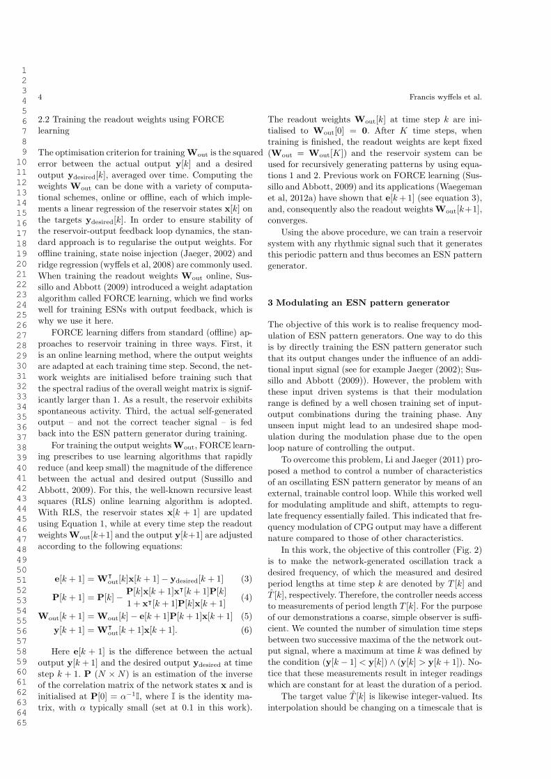
In this work, the objective of this controller (Fig. 2)is to make the network-generated oscillation track adesired frequency, of which the measured and desiredperiod lengths at time step k are denoted by T [k] andT [k], respectively. Therefore, the controller needs accessto measurements of period length T [k]. For the purposeof our demonstrations a coarse, simple observer is su"-cient. We counted the number of simulation time stepsbetween two successive maxima of the the network out-put signal, where a maximum at time k was defined bythe condition (y[k ! 1] < y[k]) # (y[k] > y[k + 1]). No-tice that these measurements result in integer readingswhich are constant for at least the duration of a period.

The target value T [k] is likewise integer-valued. Itsinterpolation should be changing on a timescale that is

1

2

3

4

5

6

7

8

9

10

11

12

13

14

15

16

17

18

19

20

21

22

23

24

25

26

27

28

29

30

31

32

33

34

35

36

37

38

39

40

41

42

43

44

45

46

47

48

49

50

51

52

53

54

55

56

57

58

59

60

61

62

63

64

65

Frequency Modulation of Large Oscillatory Neural Networks 5

!"#$%&$%'()!*+%!,

(

T

T

!

! cP Wc

!-"

!!.+

!%$#

/!"01#

"2#

2$2!

2%

2&

Fig. 2 Schematic overview of the control architecture. Forexplanation see text.

at least one order of magnitude slower than the timescaleof the individual oscillations. Comparing the measuredperiod signal with the target gives a (normalised) error

% =T [k + 1]! T [k + 1]

T [k + 1]. (7)

The control input to the reservoir is simply a biasvector Wc (N " 1) which is scaled with a constant pro-portional gain cP (a scalar that has to be tuned) and theerror % (scalar), leading to a controlled network updateequation of the form

x[k + 1] = (1! !) x[k]

+! tanh!

Wres x[k] +Wfb y[k]

+Wbias + % cP Wc

"

. (8)

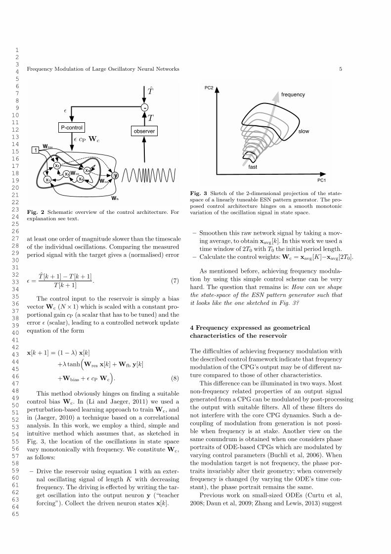
This method obviously hinges on finding a suitablecontrol bias Wc. In (Li and Jaeger, 2011) we used aperturbation-based learning approach to train Wc, andin (Jaeger, 2010) a technique based on a correlationalanalysis. In this work, we employ a third, simple andintuitive method which assumes that, as sketched inFig. 3, the location of the oscillations in state spacevary monotonically with frequency. We constitute Wc,as follows:

– Drive the reservoir using equation 1 with an exter-nal oscillating signal of length K with decreasingfrequency. The driving is e!ected by writing the tar-get oscillation into the output neuron y (“teacherforcing”). Collect the driven neuron states x[k].

!"#$

%&!'

%()*+),-.

/01

/02

Fig. 3 Sketch of the 2-dimensional projection of the state-space of a linearly tuneable ESN pattern generator. The pro-posed control architecture hinges on a smooth monotonicvariation of the oscillation signal in state space.

– Smoothen this raw network signal by taking a mov-ing average, to obtain xavg[k]. In this work we used atime window of 2T0 with T0 the initial period length.

– Calculate the control weights:Wc = xavg[K]!xavg[2T0].

As mentioned before, achieving frequency modula-tion by using this simple control scheme can be veryhard. The question that remains is: How can we shape

the state-space of the ESN pattern generator such that

it looks like the one sketched in Fig. 3?

4 Frequency expressed as geometrical

characteristics of the reservoir

The di"culties of achieving frequency modulation withthe described control framework indicate that frequencymodulation of the CPG’s output may be of di!erent na-ture compared to those of other characteristics.

This di!erence can be illuminated in two ways. Mostnon-frequency related properties of an output signalgenerated from a CPG can be modulated by post-processingthe output with suitable filters. All of these filters donot interfere with the core CPG dynamics. Such a de-coupling of modulation from generation is not possi-ble when frequency is at stake. Another view on thesame conundrum is obtained when one considers phaseportraits of ODE-based CPGs which are modulated byvarying control parameters (Buchli et al, 2006). Whenthe modulation target is not frequency, the phase por-traits invariably alter their geometry; when converselyfrequency is changed (by varying the ODE’s time con-stant), the phase portrait remains the same.

Previous work on small-sized ODEs (Curtu et al,2008; Daun et al, 2009; Zhang and Lewis, 2013) suggest

1

2

3

4

5

6

7

8

9

10

11

12

13

14

15

16

17

18

19

20

21

22

23

24

25

26

27

28

29

30

31

32

33

34

35

36

37

38

39

40

41

42

43

44

45

46

47

48

49

50

51

52

53

54

55

56

57

58

59

60

61

62

63

64

65

6 Francis wy!els et al.

0 500 1000 1500 2000 2500 3000 3500!2

!1

0

1

2Driving signal

Time step

y

0.4 0.6 0.8 1!0.8

!0.6

!0.4

!0.2

0

0.2High frequency

pc1

pc2

0.4 0.6 0.8 1!0.8

!0.6

!0.4

!0.2

0

0.2

pc1

pc2

Moderately high frequency

0.4 0.6 0.8 1!0.8

!0.6

!0.4

!0.2

0

0.2

pc1

pc2

Low frequency

Fig. 4 Driving an ESN pattern generator by a oscillationwith gradually decreasing frequency (top plot) does not causethe dynamics to simply slow down. Instead, as can be ob-served in the bottom plots, the geometrical/metric proper-ties of the phase portraits change. From left to right one canobserve that the geometry of the phase portrait is changingwhile the frequency of the teacher signal is decreased. For thethree phase portraits we used Principal Component Analysis(PCA) (Jolli!e, 2005) to obtain a 2-dimensional projection ofthe reservoir states.

that the oscillation period of half-center oscillators canbe controlled by external inputs, a mechanism whichdoes not rely on changing the time constant. To un-derstand the nature of frequency modulation of a large

non-linear dynamical system such as the discussed ESNpattern generator, we first investigate the dynamics ofESN pattern generator under external driven input.

Specifically, we inject a gradually changing oscilla-tion (y[k] = sin(0.075s[k]k), with s[k] a time dependentscaling factor which linearly decreases from 2 to 1, seetop panel in Fig. 4) through the feedback weights Wfb

of an ESN pattern generator to drive the reservoir, andrecord the reservoir states. Then we visualise the phaseportraits of this system by computing the 1st and 2ndlargest principal component (PC) of the trajectory, andplotting the projections of reservoir states on the 1st PCversus that of the 2nd PC (bottom panels in Fig. 4).From the bottom panels of this figure one can see clearlythat the phase portraits of the reservoir change in shapeand o!set across this driving input frequency-sweepingoscillation, and do so quite substantially. Details of theexperimental setup are documented in Section 6.

So it appears that when a reservoir network is pas-

sively driven by an external signal with varying fre-

quency characteristics, its excited dynamics respondswith a variation not only of its speed but also of its geo-metrical characteristics. In the remainder of this articlewe investigate whether this causation can be reversed:is it possible to modulate (only) the geometrical char-acteristics of the internal dynamics of a reservoir, havethis reservoir actively generate an output signal, andobtain a purely frequency variation in the latter? In

other words: Can we train an ESN pattern generator

such that, in state space, the oscillating signal changes

in a smooth monotonic way, i.e., its 2-dimensional pro-

jection looks similar to the sketch in Fig. 3.

The answer, as we will see, is yes. Indeed, in the casestudy that we are going to present, it is enough to adda bias of varying scale to the network dynamics in orderto obtain a geometry change that induces a frequencysweep in the output. However, implementing a robustgeometry-to-frequency causation is not without di"-culties. The main challenge that we encountered was toavoid bifurcations along the scaling route of the addi-tional bias input. The key to success turned out to bea reservoir pre-training which we termed equilibration

in earlier work (Jaeger, 2010; Li and Jaeger, 2011). Inthe next section we recapitulate the basic ideas of thistechnique.

5 Equilibration

The mechanism behind equilibration – namely, “inter-nalizing” a driven dynamics into a reservoir – has beenindependently (re-)introduced under di!erent names andfor a variety of purposes (self-prediction Mayer andBrowne (2004), equilibration Jaeger (2010), reservoirregularisation Reinhart and Steil (2012), self-sensing

networks Sussillo and Abbott (2012), innate training

Laje and Buonomano (2013)). It appears to be an RNNadaptation principle that is fundamental, versatile andsimple. In the following subsections we explain the con-cept of equilibration by a simple example, after whichwe discuss the equilibration of ESN pattern generators.

5.1 Synthetic example of equilibration

To illustrate the concept of equilibration it is helpfulto consider a simple synthetic example (repeated fromLi and Jaeger (2011)). At the top of Fig. 5 the phaseportrait of a stable circular oscillation defined in cylin-drical coordinates by r = &(!r+expx), ' = 1, x = !cx

is shown. Here r is a radius, ' an angle, and x a posi-tion. This system has a globally attracting limit cycle atx = 0, r = 1. If we would treat x as an input control pa-rameter, we would be left with a 2-dimensional systemin r and ' whose dynamics is controlled by x. Feedingx with di!erent constant values would yield stable cir-cular oscillations with radius equal to exp(x) (bottompanel). There is another way to obtain exactly the samebottom-panel phase portrait: use the 3-dimensional au-tonomous system equation

1

2

3

4

5

6

7

8

9

10

11

12

13

14

15

16

17

18

19

20

21

22

23

24

25

26

27

28

29

30

31

32

33

34

35

36

37

38

39

40

41

42

43

44

45

46

47

48

49

50

51

52

53

54

55

56

57

58

59

60

61

62

63

64

65

Frequency Modulation of Large Oscillatory Neural Networks 7

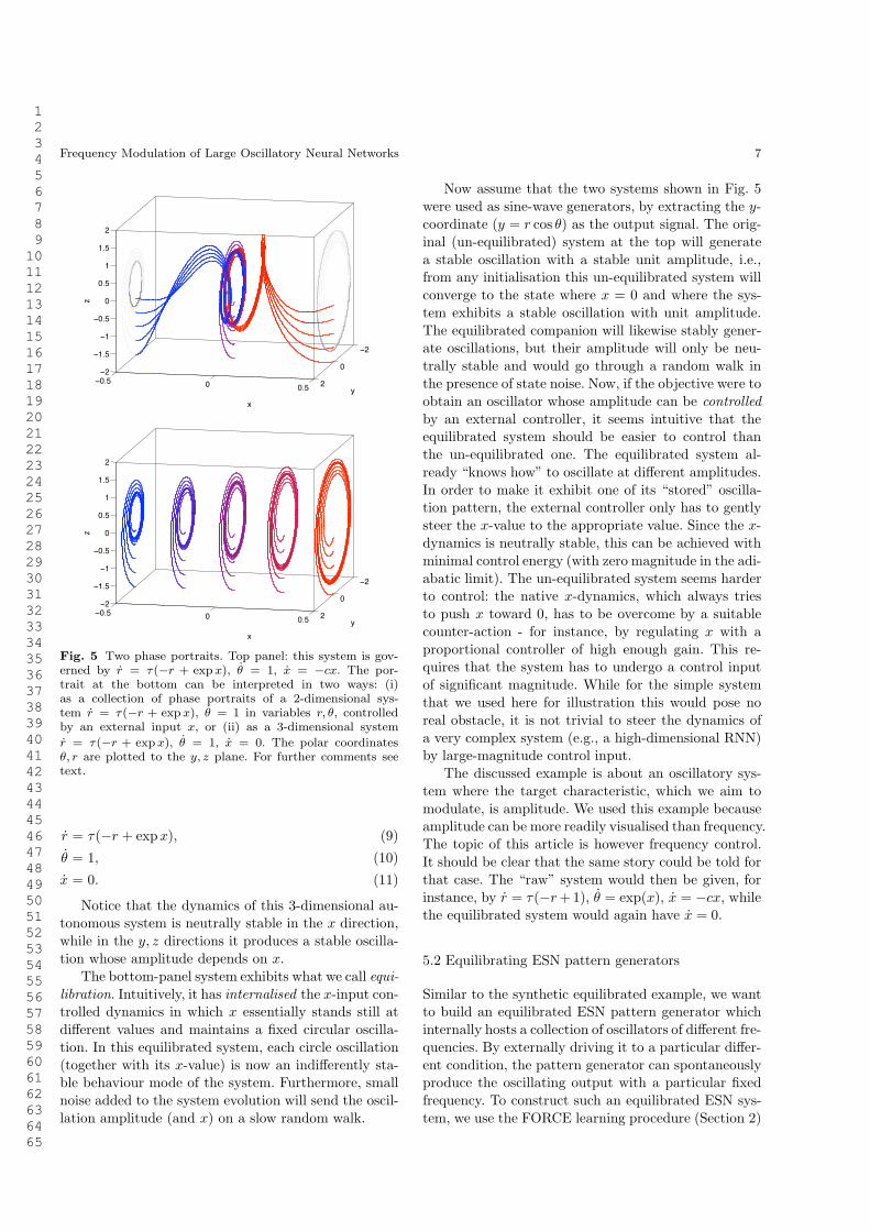
Fig. 5 Two phase portraits. Top panel: this system is gov-erned by r = τ(−r + expx), θ = 1, x = −cx. The por-trait at the bottom can be interpreted in two ways: (i)as a collection of phase portraits of a 2-dimensional sys-tem r = τ(−r + expx), θ = 1 in variables r, θ, controlledby an external input x, or (ii) as a 3-dimensional systemr = τ(−r + expx), θ = 1, x = 0. The polar coordinatesθ, r are plotted to the y, z plane. For further comments seetext.

r = &(!r + expx), (9)

' = 1, (10)

x = 0. (11)

Notice that the dynamics of this 3-dimensional au-tonomous system is neutrally stable in the x direction,while in the y, z directions it produces a stable oscilla-tion whose amplitude depends on x.

The bottom-panel system exhibits what we call equi-libration. Intuitively, it has internalised the x-input con-trolled dynamics in which x essentially stands still atdi!erent values and maintains a fixed circular oscilla-tion. In this equilibrated system, each circle oscillation(together with its x-value) is now an indi!erently sta-ble behaviour mode of the system. Furthermore, smallnoise added to the system evolution will send the oscil-lation amplitude (and x) on a slow random walk.

Now assume that the two systems shown in Fig. 5were used as sine-wave generators, by extracting the y-coordinate (y = r cos ') as the output signal. The orig-inal (un-equilibrated) system at the top will generatea stable oscillation with a stable unit amplitude, i.e.,from any initialisation this un-equilibrated system willconverge to the state where x = 0 and where the sys-tem exhibits a stable oscillation with unit amplitude.The equilibrated companion will likewise stably gener-ate oscillations, but their amplitude will only be neu-trally stable and would go through a random walk inthe presence of state noise. Now, if the objective were toobtain an oscillator whose amplitude can be controlled

by an external controller, it seems intuitive that theequilibrated system should be easier to control thanthe un-equilibrated one. The equilibrated system al-ready “knows how” to oscillate at di!erent amplitudes.In order to make it exhibit one of its “stored” oscilla-tion pattern, the external controller only has to gentlysteer the x-value to the appropriate value. Since the x-dynamics is neutrally stable, this can be achieved withminimal control energy (with zero magnitude in the adi-abatic limit). The un-equilibrated system seems harderto control: the native x-dynamics, which always triesto push x toward 0, has to be overcome by a suitablecounter-action - for instance, by regulating x with aproportional controller of high enough gain. This re-quires that the system has to undergo a control inputof significant magnitude. While for the simple systemthat we used here for illustration this would pose noreal obstacle, it is not trivial to steer the dynamics ofa very complex system (e.g., a high-dimensional RNN)by large-magnitude control input.

The discussed example is about an oscillatory sys-tem where the target characteristic, which we aim tomodulate, is amplitude. We used this example becauseamplitude can be more readily visualised than frequency.The topic of this article is however frequency control.It should be clear that the same story could be told forthat case. The “raw” system would then be given, forinstance, by r = &(!r+1), ' = exp(x), x = !cx, whilethe equilibrated system would again have x = 0.

5.2 Equilibrating ESN pattern generators

Similar to the synthetic equilibrated example, we wantto build an equilibrated ESN pattern generator whichinternally hosts a collection of oscillators of di!erent fre-quencies. By externally driving it to a particular di!er-ent condition, the pattern generator can spontaneouslyproduce the oscillating output with a particular fixedfrequency. To construct such an equilibrated ESN sys-tem, we use the FORCE learning procedure (Section 2)

1

2

3

4

5

6

7

8

9

10

11

12

13

14

15

16

17

18

19

20

21

22

23

24

25

26

27

28

29

30

31

32

33

34

35

36

37

38

39

40

41

42

43

44

45

46

47

48

49

50

51

52

53

54

55

56

57

58

59

60

61

62

63

64

65

8 Francis wy!els et al.

to build an ESN pattern generator of 1, 000 neurons andtrain the system’s readout weights Wout with a spe-cially designed target signal, namely, an oscillation witha gradually changing frequency: ydesired[k] = sin(0.075s[k]k)with s[k] a time dependent scaling factor which linearlyincreases from 1 to 3 and k from 1 to 10, 000. Fig. 6 de-picts this target signal.

An intuitive explanation for this training scheme isthat the network is trained to oscillate in di!erent fre-quencies. Consequently, when the training is successfulthe system will be able to oscillate in di!erent frequen-cies by itself. In other words, the network should con-tain a collection of oscillators of di!erent frequencies.If such a network can be made to oscillate at any fre-quency in the training range, with frequency neutrallystable (similar to amplitude in the synthetic example ofSection 5.1), this would demonstrate that we have aninstantiation of equilibration.

However, to our knowledge, with the current train-ing methods for large RNNs, only an approximatelyequilibrated system can be realised. Its hallmark wouldbe that when it is initialised to a particular frequencyby external driving, after releasing it from the drivingsignal its frequency will slowly migrate toward a pre-ferred frequency. In terms of our synthetic example (seeSection 5.1): the system from Eqns. 9 – 11 would be ap-proximately equilibrated if Eqn. 11 would for instanceread x = !(x for some small ( (or any other slow re-laxation dynamics for x).

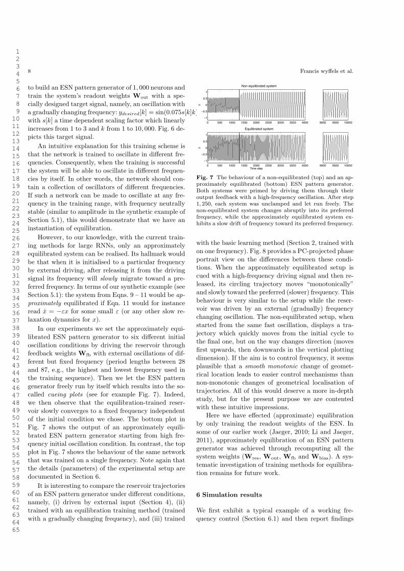
In our experiments we set the approximately equi-librated ESN pattern generator to six di!erent initialoscillation conditions by driving the reservoir throughfeedback weights Wfb with external oscillations of dif-ferent but fixed frequency (period lengths between 28and 87, e.g., the highest and lowest frequency used inthe training sequence). Then we let the ESN patterngenerator freely run by itself which results into the so-called cueing plots (see for example Fig. 7). Indeed,we then observe that the equilibration-trained reser-voir slowly converges to a fixed frequency independentof the initial condition we chose. The bottom plot inFig. 7 shows the output of an approximately equili-brated ESN pattern generator starting from high fre-quency initial oscillation condition. In contrast, the topplot in Fig. 7 shows the behaviour of the same networkthat was trained on a single frequency. Note again thatthe details (parameters) of the experimental setup aredocumented in Section 6.

It is interesting to compare the reservoir trajectoriesof an ESN pattern generator under di!erent conditions,namely, (i) driven by external input (Section 4), (ii)trained with an equilibration training method (trainedwith a gradually changing frequency), and (iii) trained

0 500 1000 1500 2000 2500 3000 3500 4000

!1

!0.5

0

0.5

1

Non equilibrated system

y

9000 9500 10000

0 500 1000 1500 2000 2500 3000 3500 4000

!1

!0.5

0

0.5

1

Equilibrated system

Time step

y

9000 9500 10000

Fig. 7 The behaviour of a non-equilibrated (top) and an ap-proximately equilibrated (bottom) ESN pattern generator.Both systems were primed by driving them through theiroutput feedback with a high-frequency oscillation. After step1, 250, each system was unclamped and let run freely. Thenon-equilibrated system changes abruptly into its preferredfrequency, while the approximately equilibrated system ex-hibits a slow drift of frequency toward its preferred frequency.

with the basic learning method (Section 2, trained withon one frequency). Fig. 8 provides a PC-projected phaseportrait view on the di!erences between these condi-tions. When the approximately equilibrated setup iscued with a high-frequency driving signal and then re-leased, its circling trajectory moves “monotonically”and slowly toward the preferred (slower) frequency. Thisbehaviour is very similar to the setup while the reser-voir was driven by an external (gradually) frequencychanging oscillation. The non-equilibrated setup, whenstarted from the same fast oscillation, displays a tra-jectory which quickly moves from the initial cycle tothe final one, but on the way changes direction (movesfirst upwards, then downwards in the vertical plottingdimension). If the aim is to control frequency, it seemsplausible that a smooth monotonic change of geomet-rical location leads to easier control mechanisms thannon-monotonic changes of geometrical localisation oftrajectories. All of this would deserve a more in-depthstudy, but for the present purpose we are contentedwith these intuitive impressions.

Here we have e!ected (approximate) equilibrationby only training the readout weights of the ESN. Insome of our earlier work (Jaeger, 2010; Li and Jaeger,2011), approximately equilibration of an ESN patterngenerator was achieved through recomputing all thesystem weights (Wres, Wout, Wfb and Wbias). A sys-tematic investigation of training methods for equilibra-tion remains for future work.

6 Simulation results

We first exhibit a typical example of a working fre-quency control (Section 6.1) and then report findings

1

2

3

4

5

6

7

8

9

10

11

12

13

14

15

16

17

18

19

20

21

22

23

24

25

26

27

28

29

30

31

32

33

34

35

36

37

38

39

40

41

42

43

44

45

46

47

48

49

50

51

52

53

54

55

56

57

58

59

60

61

62

63

64

65

Frequency Modulation of Large Oscillatory Neural Networks 9

0 1000 2000 3000 4000 5000 6000 7000 8000 9000 10000

!1

!0.5

0

0.5

1

Time step

y

Fig. 6 The signal used for equilibration training: ydesired[k] = sin(0.075s[k]k), with s[k] a time dependent scaling factorwhich linearly increases from 1 to 3.

0.4 0.6 0.8 1!0.8

!0.6

!0.4

!0.2

0

0.2Driven system

pc1

pc2

0.4 0.6 0.8 1!0.8

!0.6

!0.4

!0.2

0

0.2Equilibrated system

pc1

pc2

0.4 0.6 0.8 1!0.8

!0.6

!0.4

!0.2

0

0.2Non equilibrated system

pc1

pc2

Fig. 8 Comparison of the state evolution (projections ofthe first and second principal components of the reservoir’sstates) of a driven (left), approximately equilibrated (middle)and a non-equilibrated (right) network. For explanation seetext.

3000 4000 5000 6000 7000 8000 9000!2

!1

0

1

2

y

Generated output

3000 4000 5000 6000 7000 8000 900020

40

60

80

100

Time step

T

Measured period length

Desired

Generated

Fig. 9 Output of a frequency adjustable system (top). Thedesired frequency (light gray, bottom) goes through a slowdip and is tracked reasonably well (black curve, bottom).

from a survey of trials with a large number of randomlycreated reservoir systems (Section 6.2).

6.1 A typical example

Here, we use the reservoir system that was used through-out this paper as an example to illustrate its frequencymodulating capabilities. To recapitulate, this reservoirsystem has size N = 1, 000, a leak-rate set at 0.1 andweightsWres,Wfb andWbias respectively sampled fromnormal distributions N (0, 1), N (0, 1.5) and N (0, 0.5).The scaling factors were obtained by manual tuning.

3000 4000 5000 6000 7000 8000 9000!2

!1

0

1

2

y

Generated output

3000 4000 5000 6000 7000 8000 900040

60

80

100

Time step

T

Measured period length

Desired

Generated

Fig. 10 Output of a frequency adjustable system (top). Thecontrol target follows a random walk (bottom, target: lightgrey, measured frequency: black).

After creation of the weight matrices,Wres was rescaledsuch that the spectral radius " was set at 1.8. The read-out weights Wout were trained for equilibration witha 10, 000 step oscillation ydesired[k] = sin(0.075s[k]k)whose frequency was linearly sped up by a factor of 3by ramping s[k] from 1 to 3 (see Fig. 6 for an illustra-tion). For this, we followed the procedure outlined inSection 2. After this preparation, we verified that theequilibration was successful by visually inspecting itscueing plots. In these plots the frequency must changegradually (i.e., like the one in the bottom plot in Fig. 7).

After having obtained an approximately equilibratedreservoir, we computed the control bias Wc and acti-vated the control loop, as described in section 3. Theproportional control gain cP was determined by coarsehand-tuning. For this cP = 1 was considered as a start-ing point after which cP was decreased or increased inorder to achieve a more accurate tracking or larger con-trol range, respectively. Figs. 9 and 10 demonstrate thatfrequency could be controlled in a range of a factor 3.

6.2 From equilibration to modulatability

The equilibration procedure does not always result ina system which behaves as “smoothly” as shown inFigs. 7 (bottom) and 8 (middle). We found two con-ditions which impede subsequent controllability. First,

1

2

3

4

5

6

7

8

9

10

11

12

13

14

15

16

17

18

19

20

21

22

23

24

25

26

27

28

29

30

31

32

33

34

35

36

37

38

39

40

41

42

43

44

45

46

47

48

49

50

51

52

53

54

55

56

57

58

59

60

61

62

63

64

65

10 Francis wy!els et al.

it occurs that the equilibration-trained system escapesinto aperiodic (presumably chaotic) or fixed-point dy-namics. These systems are not able to maintain a fixedfrequency oscillation and consequently are not suitable.Second, even if the equilibration-trained system exhibitsperiodic behaviour and has only a single preferred fre-quency, convergence toward this frequency from othercueing frequencies may be too strong (e.g., Figs 7 (top)and 8 (right)). For these systems, the equilibration workedout to an insu"cient degree. Consequently, these sys-tems can not be frequency-controlled by using a simplelinear controller.

We carried out a two-stage screening, starting froma population of 20, 000 randomly created reservoirs.From these, we first discarded the ones that showedaperiodic or fixed-point behaviour, and in a second stepthe ones that showed an insu"cient degree of equili-bration. The ones that were left over were tested forcontrollability.

Specifically, the 20, 000 raw reservoirs, similar tosubsection 6.1, all had 1, 000 neurons and a leak-rateof 0.15. The spectral radius ", feedback scaling o andbias # scaling was set at 1.8, 1.5 and 0.5 respectively.Each of these reservoirs was then equilibration-trainedas described in subsection 5.2. Each system thus pre-pared was then cued with six oscillations whose periodsspanned the training range of 28 to 87 steps. After cue-ing for 1, 250 steps, the system was let run freely until10, 000 time steps were passed. We assumed that con-vergence to any preferred dynamic mode would occurwithin this runtime.

For each pattern generator we first checked whetherall of its six free runs converged to a fixed frequency os-cillation. Therefore, we removed all systems which freerun let to a fixed point or aperiodic behaviour.

Next, we checked whether the equilibration had workedout in the desired fashion, ideally looking like the bot-tom plot in Fig. 7.

In order to automatically glean systems which havethe desired “smooth and slow” transient from a cuedperiod length toward the preferred one, we employedthe following heuristic. From among the six cueing runswe used the one that started from the highest (period28) and the lowest (period 87) frequency. From the gen-erated time series, we obtained the evolution of periodlengths T1, ..., Ti, ..., TK (e.g., Fig. 11) with TK the lastmeasured period length from the free run. The sequenceT1, ..., Ti, ..., TK was then smoothed by a moving aver-age filter. From the smoothed sequence, we calculatedheuristic measures ), * , + for speed of convergence,

0 10 20 30 40 50 60 70 80 90 1000

50

100

T

Approximately equilibrated

0 10 20 30 40 50 60 70 80 90 10020

40

60

80

T

Non equilibrated

0 10 20 30 40 50 60 70 80 90 10020

40

60

Number of periods

T

Non equilibrated

Fig. 11 Three examples of period length transient dynamicsfrom a (cued) short period to a (preferred) longer period.Plots show progression of period length against number ofperiods. Only the example in the top plot exhibits the desiredquasi-linear ramping-up.

curvature and monotonicity, respectively:

) = max|Ti+1 ! Ti| for $i = 1...K ! 1 (12)

* = max|(Ti+1 ! Ti)! (Ti ! Ti!1)| (13)

for $i = 2...K ! 1

+ =K!1#

i=2

|sgn(Ti+1 ! Ti)! sgn(Ti ! Ti!1)| (14)

We considered a period sequence T1, ..., Ti, ..., TK asproof of a successful equilibration if it was monotonic(in the sense that + = 0), not too steep () < 2.0) andnot too curved (* < 0.2).

Out of the 20, 000 systems, 1, 573 remained after ourselection procedure. All 1, 573 systems were found fre-quency adjustable which was determined by the meanabsolute error (MAE) between the desired period lengthsand the observed period lengths. The same target as inFig. 9 was used and the threshold for acceptance was setat MAE = 4.0. In roughly half of the cases the defaultinitial proportional gain cP, which was obtained afterrough manual tuning in the example from Section 6.1,was su"cient to meet the objective. In the other cases,manual tuning of cP was necessary.

These empirical results show that frequency mod-ulation can be realised in high dimensional non-linearpattern generators provided that they are successfully(approximately) equilibrated.

7 Discussion

In this contribution we argued that

– biological and robotic pattern generators need to beadjustable in many ways, and

1

2

3

4

5

6

7

8

9

10

11

12

13

14

15

16

17

18

19

20

21

22

23

24

25

26

27

28

29

30

31

32

33

34

35

36

37

38

39

40

41

42

43

44

45

46

47

48

49

50

51

52

53

54

55

56

57

58

59

60

61

62

63

64

65

Frequency Modulation of Large Oscillatory Neural Networks 11

– modulation of speed di!ers fundamentally frommod-ulation of other, “geometric” characteristics, and

– richly trainable and adjustable pattern generatorsare likely to require neural networks of substantialsize, –

– which leads to the question of generic mechanismsfor frequency control of neural pattern generators.

Here we considered the special case of oscillatorynetworks, and demonstrated that their frequency canbe made controllable by

– training the network in a way that it is forced toadapt its weights to accommodate to a range of fre-quencies (“equilibration”),

– which, if is successful, results in a monotonic inter-dependence between temporal and spatial proper-ties of the network dynamics,

– which in turn can be exploited for controlling timeby spatial state shifts through a bias term in a pro-portional control loop.

Our study is a proof of principle, with many de-sign decisions made ad hoc. Variations and extensionso!er themselves in many ways, e.g., improved controlschemes (for example, PID controllers instead of simpleP controllers, or making the bias weightsWc frequency-dependent), more sophisticated observers for frequency,other equilibration methods (for instance, training allreservoir weights instead of training only the outputweights, as done in Jaeger (2010)), investigating othersignal shapes, etc. Furthermore, in our groups we alsoinvestigate altogether di!erent learning architecturesfor making frequency adjustable ESN pattern gener-ators. For instance, in (Jaeger, 2007) a multifrequencygenerator is directly trained as an open-loop controlsystem. Thus, the present study does not claim to o!erthe solution for constructing large frequency adjustableoscillatory neural networks. We nonetheless considerthe following as relevant contributions:

– pointing out the importance and di"culty of theneural speed control problem in the first place,

– clarifying the existence and functional role of equili-bration of dynamics for making selected character-istics robustly controllable, and

– demonstrating that a temporal – spatial interdepen-dency of trajectories can be shaped and exploitedfor control.

Biological evolution is likely to adopt whatever workswell. Biological research has identified frequency controlmechanisms in small CPG model systems which relyon specific, idiosyncratic mechanisms. Roboticists sim-ply adapt the speed of ODE based pattern generators

by changing the time constants. The work presented inthis article does not aim at replacing or refuting any ofthese insights or techniques. However, in higher corti-cal processing domains in biological systems, or in flex-ibly trainable RNN-based robotic control modules, weperceive an arena where generic neural speed controlschemes such as the one illustrated in this work mightbecome important.

Acknowledgements The authors would like to thank theanonymous reviewers for their constructive comments thathelped improving this manuscript. The research leading tothe results presented here has received funding from the Eu-ropean Community’s Seventh Framework Programme (EUFP7) under grant agreement n.248311 Adaptive Modular Ar-chitecture for Rich Motor Skills (AMARSi).

References

Briggman K, Kristan Jr W (2006) Imaging dedi-cated and multifunctional neural circuits generat-ing distinct behaviors. The Journal of Neuroscience26:10,925–10,933

Briggman K, Kristan Jr W (2008) Multifuctionalpattern-generating circuits. Annual Review of Neu-roscience 31:271–294

Buchli J, Righetti L, Ijspeert A (2006) Engineering en-trainment and adaptation in limit cycle systems. Bi-ological Cybernetics 95:645–664

Buschges A, Scholz H, El Manira A (2011) New movesin motor control. Current Biology 21:R513–R524

Caluwaerts K, D’Haene M, Verstraeten D, Schrauwen B(2013a) Locomotion without a brain: Physical reser-voir computing in tensegrity structures. Artificial Life19:35–66

Caluwaerts K, wy!els F, Dieleman S, Schrauwen B(2013b) The spectral radius remains a valid indica-tor of the echo state property for large reservoirs. In:Proceedings of the International Joint Conference onNeural Networks

Cruse H, Brunn D, Bartling C, Dean J, Dreifert M,Kindermann T, Schmitz J (1995) Walking: A com-plex behavior controlled by simple networks. Adap-tive Behavior 3(4):385–418

Curtu R, Shpiro A, Rubin N, Rinzel J (2008) Mecha-nisms for frequency control in neuronal competitionmodels. SIAM Journal on Applied Dynamical Sys-tems 7:609–649

Daun S, Rubin J, Rybak I (2009) Control of oscillationperiods and phase durations in half-center centralpattern generators: a comparative mechanistic anal-ysis. Journal of Computational Neuroscience 27:3–36

Dean J, Kindermann T, Schmitz J, Schumm M, CruseH (1999) Control of walking in the stick insect: From

1

2

3

4

5

6

7

8

9

10

11

12

13

14

15

16

17

18

19

20

21

22

23

24

25

26

27

28

29

30

31

32

33

34

35

36

37

38

39

40

41

42

43

44

45

46

47

48

49

50

51

52

53

54

55

56

57

58

59

60

61

62

63

64

65

12 Francis wy!els et al.

behavior and physiology to modeling. AutonomousRobots 7:271–288

Fukuoka Y, Kimura H, Cohen A (2003) Adaptive dy-namic walking of a quadruped robot on irregular ter-rain based on biological concepts. The InternationalJournal of Robotics Research 22:187–202

Grillner S (1985) Neurobiological bases of rhythmic mo-tor acts in vertebrates. Science 228:143–149

Ijspeert A (2008) Central pattern generators for loco-motion control in animals and robots: a review. Neu-ral Networks 21:642–653

Ijspeert A, Crespi A, Ryczko D, Cabelguen JM(2007) From swimming to walking with a salaman-der robot driven by a spinal cord model. Science315(5817):1416–1420

Ijspeert A, Nanaishi J, Ho!mann H, Pastor P, SchaalS (2013) Dynamical movement primitives: Learningattractor models for motor behaviors. Neural Com-putation 25:328–373

Jaeger H (2001) The “echo state” approach to analysingand training recurrent neural networks. Gmd report148, German National Research Center for Informa-tion Technology

Jaeger H (2002) A tutorial on training recurrent neuralnetworks, covering bppt, rtrl, ekf and the ”echo statenetwork” approach. Gmd report 159, InternationalUniversity Bremen

Jaeger H (2007) Echo state network. In: Scholarpedia,vol 2, p 2330, URL http://www.scholarpedia.org/

article/Echo_State_Network

Jaeger H (2010) Reservoir self-control for achieving in-variance against slow input distortions. Technical re-port 23, Jacobs University Bremen

Jolli!e I (2005) Principal Component Analysis. Ency-clopedia of Statistics in Behavioral Science.

Laje R, Buonomano DV (2013) Robust timing and mo-tor patterns by taming chaos in recurrent neural net-works. Nature Neuroscience 16(7):925–933

Li J, Jaeger H (2011) Minimal energy control of an ESNpattern generator. Technical report 26, Jacobs Uni-versity Bremen, School of Engineering and Science

Lukosevicius M (2012) A practical guide to applyingecho state networks. Neural Networks: Tricks of theTrade, Reloaded 7700:659–686

Lukosevicius M, Jaeger H (2009) Reservoir comput-ing approaches to recurrent neural network training.Computer Science Review 3:127–149

Mayer NM, Browne M (2004) Echo state networks andself-prediction. In: Biologically Inspired Approachesto Advanced Information Technology, LNCS, vol3141, Springer Verlag Berlin / Heidelberg, pp 40–48

Nakanishi J, Morimoto J, Endo G, Chenga G, SchaalS, Kawato M (2004) Learning from demonstration

and adaptation of biped locomotion. Robotics andAutonomous Systems 47:79–91

Reinhart R, Steil J (2011) A constrained regularizationapproach for input-driven recurrent neural networks.Di!erential Equations and Dynamical Systems 19(1–2):27–46

Reinhart R, Steil J (2012) Regularization and stabilityin reservoir networks with output feedback. Neuro-computing 90:96–105

Reinhart R, Steil JJ (2008) Recurrent neural associa-tive learning of forward and inverse kinematics formovement generation of the redundant pa-10 robot.In: Proceedings of the ECSIS Symposium on Learn-ing and Adaptive Behaviors for Robotic Systems, pp35–40

Rolf M, Steil JJ, Gienger M (2010a) Goal babblingpermits direct learning of inverse kinematics. IEEETransactions on Autonomous Mental Development2(3):216–229

Rolf M, Steil JJ, Gienger M (2010b) Learning flexiblefull body kinematics for humanoid tool use. In: Pro-ceedings of the International Symposium on Learningand Adaptive Behavior in Robotic Systems

Schrauwen B, Defour J, Verstraeten D, Van Camp-enhout J (2007) The introduction of time-scales inreservoir computing, applied to isolated digits recog-nition. In: Proceedings of the International Confer-ence on Artificial Neural Networks

Sussillo D, Abbott L (2012) Transferring learning fromexternal to internal weights in echo-state networkswith sparse connectivity. PLoS ONE 7(5):e37,372

Sussillo D, Abbott LF (2009) Generating coherent pat-terns of activity from chaotic neural networks. Neu-ron 63:544–557

Verstraeten D, Schrauwen B, D’Haene M, Stroobandt D(2007) An experimental unification of reservoir com-puting methods. Neural Networks 20:391–403

Waegeman T, Schrauwen B (2011) Towards learning in-verse kinematics with a neural network based track-ing controller. In: Lecture Notes in Computer Sci-ence, vol 7064, pp 441–448

Waegeman T, wy!els F, Schrauwen B (2012a) Feed-back control by online learning an inverse models.IEEE Transactions on Neural Networks and Learn-ing Systems 23:1637–1648

Waegeman T, wy!els F, Schrauwen B (2012b) A re-current neural network based discrete and rhythmicpattern generator. In: Proceedings of the EuropeanSymposium on Artificial Neural Networks

Waegeman T, wy!els F, Schrauwen B (2012c) Towardsa neural hierarchy of time scales for motor control.In: Lecture Notes in Computer Science, vol 7426, pp146–155

1

2

3

4

5

6

7

8

9

10

11

12

13

14

15

16

17

18

19

20

21

22

23

24

25

26

27

28

29

30

31

32

33

34

35

36

37

38

39

40

41

42

43

44

45

46

47

48

49

50

51

52

53

54

55

56

57

58

59

60

61

62

63

64

65

Frequency Modulation of Large Oscillatory Neural Networks 13

Wrede S, Johannfunke M, Nordmann A, Ruther S,Weirich A, Steil J (2010) Interactive learning of in-verse kinematics with nullspace constraints using re-current neural networks. In: Proceedings of the 20thWorkshop on Computational Intelligence

wy!els F, Schrauwen B (2009) Design of a central pat-tern generator using reservoir computing for learninghuman motion. In: Proceedings of the ECSIS Sympo-sium on Advanced Technologies for Enhanced Qual-ity of Life, pp 118–122

wy!els F, Schrauwen B, Stroobandt D (2008) Stableoutput feedback in reservoir computing using ridgeregression. In: Proceedings of the International Con-ference on Analog Neural Networks

Yildiz I, Jaeger H, Kiebel S (2012) Re-visiting the echostate property. Neural Networks 35:1–9

Zhang C, Lewis T (2013) Phase response propertiesof half-center oscillators. Journal of ComputationalNeuroscience 35:55–74

1

2

3

4

5

6

7

8

9

10

11

12

13

14

15

16

17

18

19

20

21

22

23

24

25

26

27

28

29

30

31

32

33

34

35

36

37

38

39

40

41

42

43

44

45

46

47

48

49

50

51

52

53

54

55

56

57

58

59

60

61

62

63

64

65