f n) = h n) + g n f n g n found so fardjmoon/ai/ai-notes/search-heuristic.pdf · { path-cost has...

Heuristic Search: Intro

• Blind search can be applied to all problems

• Is inefficient, as does not incorporate knowledge about the problem to guidethe search

• Such knowledge can be used when deciding which node to expand next

• Heuristic search (aka informed, best first search) uses problem knowledge toselect state that appears to be closest to goal state as next to expand

• This should produce a solution faster than systematically expanding all nodestil a goal is stumbled upon

• The general state evaluation function: f(n) = h(n) + g(n)

– f(n)) is estimated cost of getting from start state to goal state via state n

– g(n) is actual cost of getting from start state to n found so far

– h(n) is heuristic function: estimated cost of going from n to goal state

∗ This function is where knowledge about the problem comes into play

∗ h(goal) = 0

– f ∗(n) = h∗(n) + g∗(n) represents the minimal cost of getting from startstate to goal state via state n when all paths through n are considered

∗ h∗(n) is actual cost to goal from n

∗ g∗(n) is cost of best path to n from initial state

• There are categories of heuistic search, based on variations in f(n))

1

Heuristic Search: Intro (2)

• General algorithm (tree):

function GIS-TREE (problem, evalFn) returns solution, or failure

{

node <- new(node)

node.STATE <- problem.INITIAL-STATE

node.COST <- apply(evalFn, INITIAL-STATE)

frontier <- new(priorityQueue)

INSERT(node, frontier)

explored <- new(set)

loop {

if (EMPTY?(frontier))

return failure

node <- POP(frontier)

if (problem.GOAL-TEST(node.STATE))

return SOLUTION(node)

for (each action in problem.ACTIONS(node.STATE)) {

child <- CHILD-NODE(problem, node, action)

frontier <- INSERT(child, frontier)

}

}

}

2


• General algorithm (graph):

function GIS-GRAPH (problem, evalFn) returns solution, or failure

{

node <- new(node)






loop {


return failure




ADD(node.STATE, explored)



if ((child.STATE !in explored) AND

((!STATE-FOUND(child.STATE, frontier)) {


else if (STATE-FOUND(child.STATE, frontier)) {

node <- RETRIEVE-NODE(child.STATE, frontier)

if (child.COST < node.COST))

frontier <- REPLACE(node, child, frontier)

}

}

}

}

3


– The above is a modified version of the uniform cost algorithm

– it accepts an additional argument: the function used to assign a value to anode

– Function apply(function, node) evaluates function for a given node

– PATH-COST has been replaced by a more generic PATH attribute

– Attributes that need to be stored on a node are dependent on the searchstrategy

4

Heuristic Search: Greedy Search

• The greedy search algorithm selects the node that appears to be closest to thegoal

– f(n) = h(n)

– I.e., g(n) = 0: We ignore cost to get to a node

• Algorithm GS:

function GS (problem) returns solution, or failure

{

return GIS-TREE (problem, h)

// OR return GIS-GRAPH (problem, h)

}

• Characteristics:

– Attempts to get to goal as quickly as possible

– May reach dead ends

– May expand nodes unnecessarily

– Not complete for tree rep (due to reversible actions)

– Complete for graph rep of finite state space

– Not optimal

• Complexity:

– Storage requirements ∈ O(bd) (where d is max depth of structure

– Time requirements ∈ O(bd)

• Note that quality of heuristic greatly affects search

5

Heuristic Search: A∗

• Combines aspects of uniform cost and greedy seraches

– UCS is optimal and complete, but inefficient

– UCS based on g(n)

– GS is neither optimal nor complete, but efficient

– GS based on h(n)

– For A∗, f(n) = h(n) + g(n)

• Algorithm A∗ (for trees)

function ASTAR-TREE (problem) returns solution, or failure

{

return GIS-TREE (problem, h + g)

}

• A∗ is optimal and complete, providing that

1. For trees, h(n) is admissible

– Admissible means that h(n) ≤ h∗(n)

– I.e., h(n) never over-estimates cost from n to g

– Such an algorithm is optimistic

2. For graphs, h(n) is consistant (monotonic)

– h(n) is consistant if for every node n and successor nodes n′ generatedby action a, the estimated cost of getting from n to the goal is nevergreater than the actual cost of getting fom n to a successor state n′ plusthe estimated cost of getting from n′ to the goal

– I.e., h(n) ≤ c(n, a, n′) + h(n′) for all n′

6

Heuristic Search: A∗ (2)

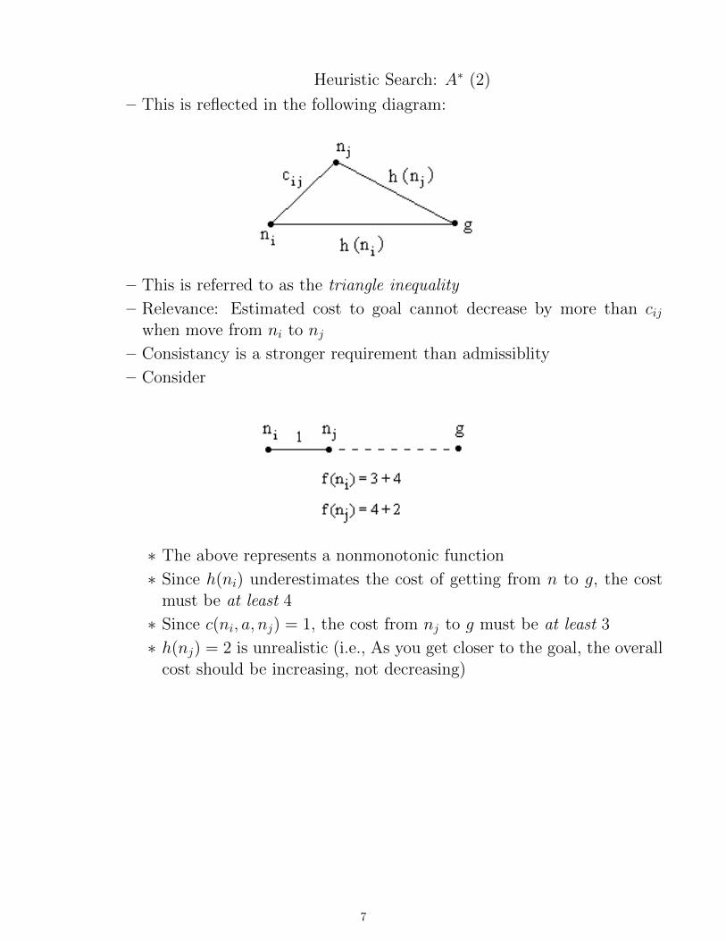
– This is reflected in the following diagram:

– This is referred to as the triangle inequality

– Relevance: Estimated cost to goal cannot decrease by more than cijwhen move from ni to nj

– Consistancy is a stronger requirement than admissiblity

– Consider

∗ The above represents a nonmonotonic function

∗ Since h(ni) underestimates the cost of getting from n to g, the costmust be at least 4

∗ Since c(ni, a, nj) = 1, the cost from nj to g must be at least 3

∗ h(nj) = 2 is unrealistic (i.e., As you get closer to the goal, the overallcost should be increasing, not decreasing)

7

Heuristic Search: A∗ Graphs

• As with blind search, using graphs instead of trees will result in extra effort

• Handling already-visited nodes more complex in A∗

– When encounter node that appears on frontier or closed, may have foundan alternate path to the node

– New path may be cheaper than original

∗ If new path is not cheaper, just ignore newly found path

∗ If not, must adjust f of the node, and adjust path pointers between itand parent

∗ If the node is on closed, will also have to cascade updated cost of paththrough descendants

8

Heuristic Search: A∗ Graphs (2)

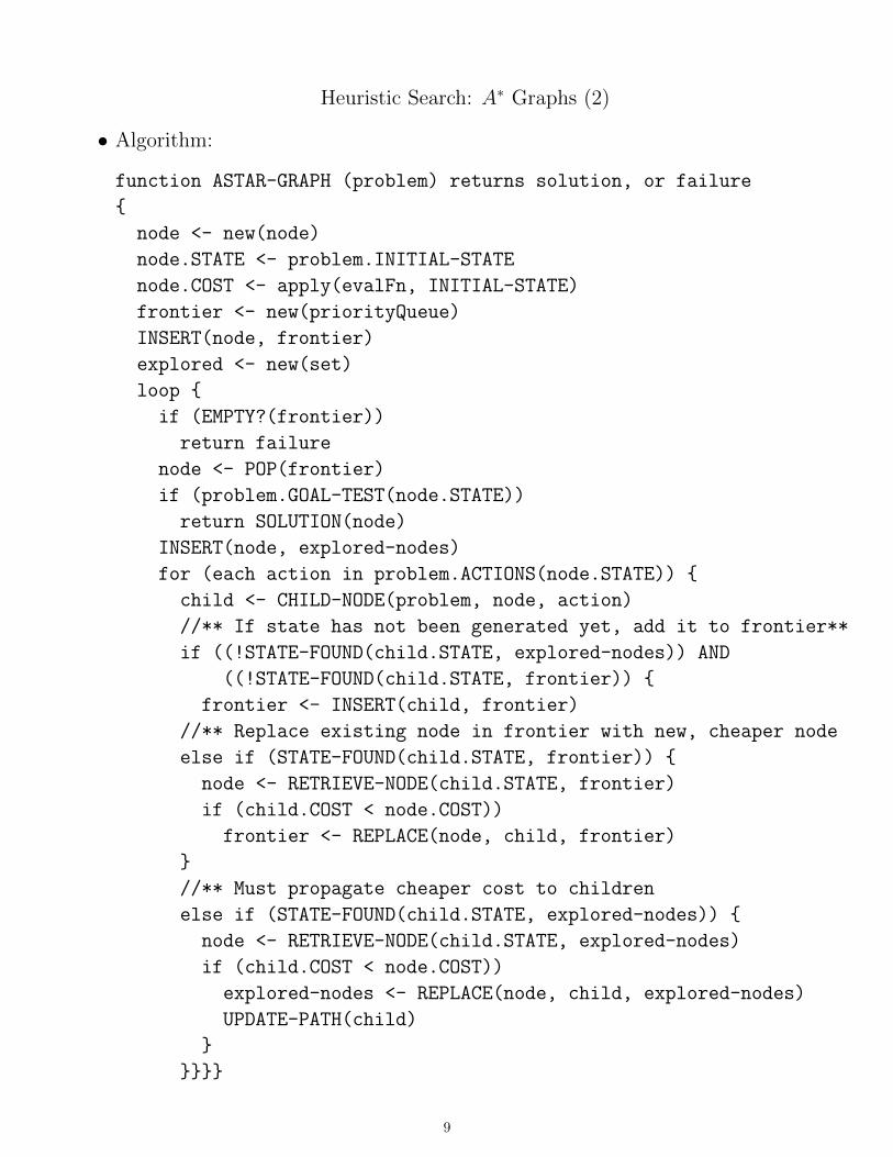
• Algorithm:

function ASTAR-GRAPH (problem) returns solution, or failure

{

node <- new(node)






loop {


return failure




INSERT(node, explored-nodes)



//** If state has not been generated yet, add it to frontier**

if ((!STATE-FOUND(child.STATE, explored-nodes)) AND

((!STATE-FOUND(child.STATE, frontier)) {


//** Replace existing node in frontier with new, cheaper node

else if (STATE-FOUND(child.STATE, frontier)) {

node <- RETRIEVE-NODE(child.STATE, frontier)


frontier <- REPLACE(node, child, frontier)

}

//** Must propagate cheaper cost to children

else if (STATE-FOUND(child.STATE, explored-nodes)) {

node <- RETRIEVE-NODE(child.STATE, explored-nodes)


explored-nodes <- REPLACE(node, child, explored-nodes)

UPDATE-PATH(child)

}

}}}}

9

Heuristic Search: A∗ Graphs (3)

– Note that this algorithm is essentially the same as GIS-GRAPH, except fortwo changes:

1. The last if-else:

else if (child.STATE in explored)

UPDATE-PATH(child)

∗ If child appears in explored, this means that it has been expandedand we have generated any number of ancestors for this state

∗ If we have found a cheaper path to child, then the cost associatedwith those ancestors will need to be adjusted, since the paths to theancestors go through child

∗ Function UPDATE-PATH will id those states reached via child

· These nodes may be in frontier or explored-nodes

· The g values will be updated (to a lesser value), which will decreasetheir f values

2. explored-nodes

∗ The text’s formulation maintains states - not nodes - on the exploredlist

∗ Since A∗ graph search requires us to be able to adjust costs and tra-verse paths to explored nodes, we must retain nodes - not just stateinformation - on the explored list

∗ The name explored-nodes emphasizes this change from graph searchalgorithms presented earlier

10

Heuristic Search: A∗ Optimality

• This examines the optimality of A∗ graph search

1. If h(n) is consistant, then values of f(n) are nondecreasing along any path

Given g(n′) = g(n) + c(n, a, n′)

Then, f(n′) = g(n′)+h(n′) = g(n)+c(n, a, n′)+h(n′) ≥ g(n)+h(n) =f(n)

2. At every step prior to termination of A∗, there is always a node n∗ onfrontier with the following properties:

– n∗ is on optimal path to a goal

– A∗ has found an optimal path to n∗

– f(n∗) ≤ f ∗(n0)

3. Proof (by induction):

(a) Base case:

– At start, only n0 on frontier

– n0 on optimal path to goal

– f(n∗) ≤ f(n0) = h(n0∗)(b) Inductive assumption:

– Assume m ≥ 0 nodes expanded and above holds for each

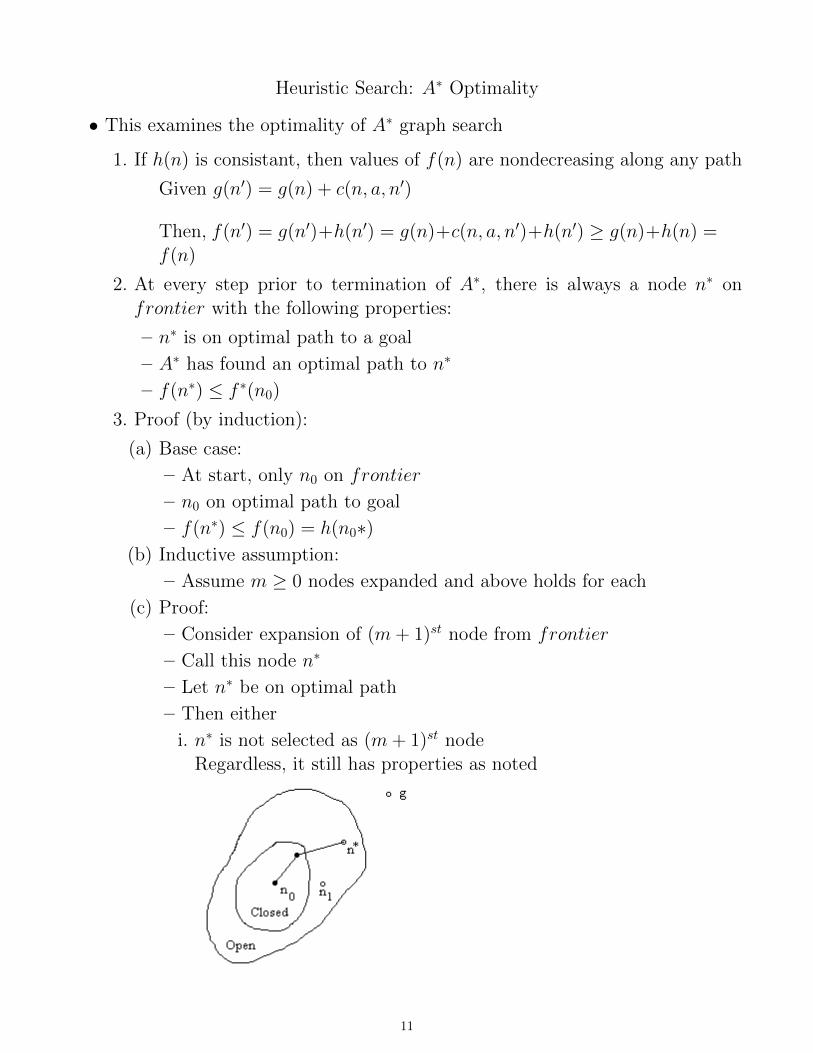
(c) Proof:

– Consider expansion of (m+ 1)st node from frontier

– Call this node n∗

– Let n∗ be on optimal path

– Then either

i. n∗ is not selected as (m+ 1)st nodeRegardless, it still has properties as noted

11

Heuristic Search: A∗ Optimality (2)

ii. n∗ is selected

– In the second case, let np be one of n∗’s successors on an optimal path

– This node is on frontier

– Path to np must be optimal, otherwise, there would be a better pathto the goal

– np becomes the new n∗ for the next iteration of the algorithm

(d) Proof that f(n∗) ≤ f(n0)

– Let n∗ be on optimal path and assume A∗ has found optimal pathfrom n0 to n∗

– Then

f(n∗) = g(n∗) + h(n∗) (1)

≤ g(n∗) + h(n∗) (since g(n∗) = g(n∗) and h(n∗) ≤ h(n∗)(2)

≤ f(n∗) (since f(n∗) = g(n∗) + h(n∗)) (3)

≤ f(n0) (since f(n∗) = f(n0) and n∗ on optimal path) (4)

(5)

12


4. Given the conditions specified for A∗ and h, and providing there is a pathwith finite cost from n0 to goal, A∗ is guaranteed to terminate with aminimal cost path to a goal

5. Proof (by contradiction): A∗ terminates if there is an accessible goal

– Assume A∗ doesn’t terminate

– Then a point will be reached where f(n) > f(n0) for some n ∈ frontier,since ε > 0

– This contradicts assumption

6. Proof (by contradiction): Termination of A∗

(a) A∗ terminates when either frontier empty

– This contradicts assumption that there is an accessible goal

(b) Or when a goal node is id’d

– Suppose there is an optimal goal g1 where f(g1) = f(n0),and A∗ finds a non-optimal goal g2 with f(g2) > f(n0) where g1 6= g2

– When A∗ terminates, f(g2) ≥ f(g2) > f(n0)

– But prior to selection of g2, there was a node n∗ on frontier on anoptimal path with f(n∗) ≤ f(n0) by previous lemma

– This contradicts assumptions

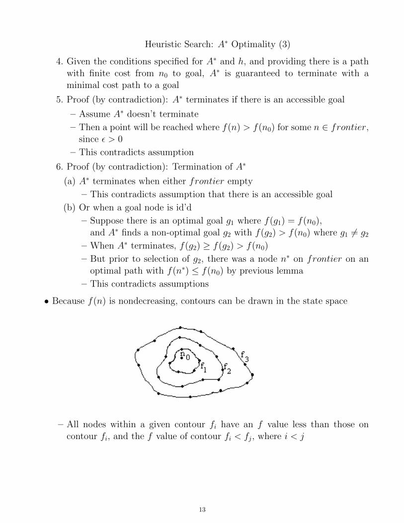
• Because f(n) is nondecreasing, contours can be drawn in the state space

– All nodes within a given contour fi have an f value less than those oncontour fi, and the f value of contour fi < fj, where i < j

13


– As the search progresses, the contours narrow and stretch toward the goalalong the cheapest path

– The more accurate h(n), the more focused the contours become

– Note that UCS generates circular contours centered on the initial state

• A∗ is optimally efficient for any given h function:

– No other algorithm is guaranteed to expand fewer nodes than A∗

14

Heuristic Search: A∗ Complexity

• The number of states within the goal contour is exponential wrt the solutionlength

• For problems of constant step costs, analysis is based on

1. Absolute error: ∆ = h∗ − h2. Relative error: ε = (h∗ − h)/h∗

• Complexity analysis depends on the characteristics of the state space

• When there is a single goal and reversible actions

– Time complexity ∈ O(b∆) = O(bεd), where d is the solution depth

– For heuristics of practical use, ∆ ∝ h∗, so ε is constant or growing and timecomplexity is exponential in d

– O(bεd) = O((bε)d) which means the effective branching factor is bε

• If there are many goal states (especially near-optimal goal states), path mayveer from the optimal path

– This will result in additional cost proportional to the number of goal stateswithin a factor of ε of the optimal cost

• With a graph, there can be exponentially many states with f(n) < C∗

• The search usually runs out of space before time becomes an issue

15

Heuristic Search: Variations to A∗

• The main issue with A∗ is memory usage

– As noted above, the algorithm usually uses up available memory beforetime becomes an issue

• The following algorithms attempt to limit memory usage while retaining theproperties of A∗

16

Heuristic Search: Variations to A∗ - Iterative Deepening A∗ Search (IDA∗)

• This is the A∗ version of the depth first iterative deepening algorithm

– On each iteration, perform a ”depth first” search

– Instead of using a depth limit, use a bound on f

• Algorithm IDA∗

function IDASTAR (problem) returns solution, or failure

{

root <- new(node)

root.STATE <- problem.INITIAL-STATE

root.FCOST <- problem.GET-INITIAL-STATE-H()

f-limit <- root.FCOST

while (TRUE) {

[result, f-limit] <- DFS-CONTOUR(root, problem, f-limit)

if (result != NULL)

return result

else if (f-limit == infinity)

return failure

}

function DFS-CONTOUR (node, problem, f-limit) returns [solution, f-limit]

{

nextF <- infinity

if (node.FCOST > f-limit)

return [node, node.FCOST]


return [node, f-limit]



[solution, newF] <- DFS-CONTOUR(child, f-limit)

if (solution NOT NULL)

return [solution, f-limit]

nextF <- min(nextF, newF)

}

return [NULL, nextF]

17

Heuristic Search: Variations to A∗ - Iterative Deepening A∗ Search (IDA∗) (2)

• Expands nodes along contour lines of equal f

• IDA∗ complete and optimal

• Complexity

1. Space

– Let δ = smallest operator cost

– Let f ∗ = optimal solution cost

– Worst case requires bf∗

δ nodes

2. Time

– Dependent on range of values that f can assume

– Best case

∗ The fewer the values, the fewer the contours ⇒ fewer iterations

∗ Thus, IDA∗ → A∗

∗ Also has less overhead as does not require priority queue

– Worst case

∗ When have many unique values for h(n) (absolute worst is every hvalue unique)

∗ Requires many iterations

∗ ∼ 1 + 2 + ...+ n ∈ O(n2)

• To reduce time complexity

– increase f − limit by ε on every iteration

– Number of iterations ∝ 1/ε

– While reduces search cost, may produce non-optimal solution

– Such a solution is worse than optimal by at most ε

– Such algorithms called ε-admissible

18

Heuristic Search: Variations to A∗ - Recursive Best First Search (RBFS)

• This uses more memory than IDA∗ but generates fewer nodes

• Uses same approach as A∗ with following differences

– Assigns a backed up value to each node

∗ Let n be a node with mi successors

∗ Backed up value of n = b(n) = min(b(mi))

∗ Backed up value of leaf node (one on frontier) is f(n)

∗ Backed up value of a node represents descendant with lowest f value intree rooted at node

– Only most promising path to goal maintained at any time

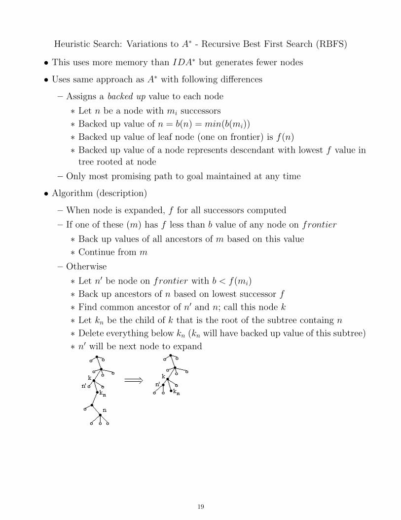
• Algorithm (description)

– When node is expanded, f for all successors computed

– If one of these (m) has f less than b value of any node on frontier

∗ Back up values of all ancestors of m based on this value

∗ Continue from m

– Otherwise

∗ Let n′ be node on frontier with b < f(mi)

∗ Back up ancestors of n based on lowest successor f

∗ Find common ancestor of n′ and n; call this node k

∗ Let kn be the child of k that is the root of the subtree containg n

∗ Delete everything below kn (kn will have backed up value of this subtree)

∗ n′ will be next node to expand

19

Heuristic Search: Variations to A∗ - Recursive Best First Search (RBFS) (2)

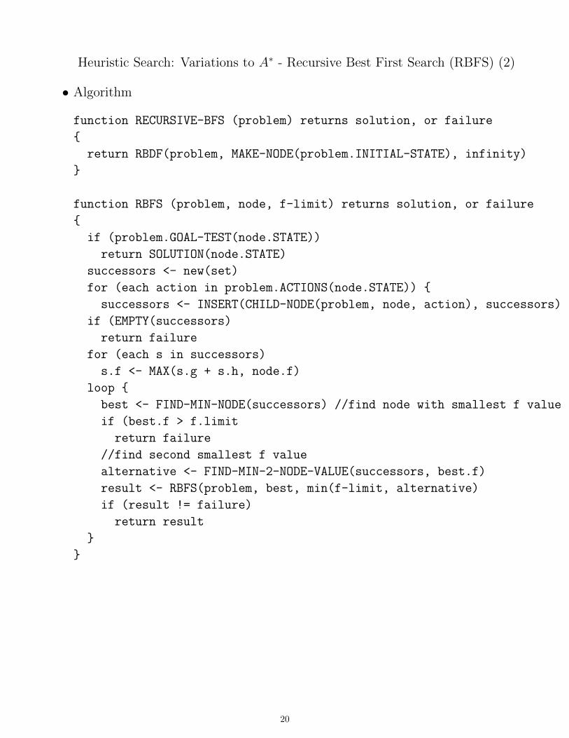
• Algorithm

function RECURSIVE-BFS (problem) returns solution, or failure

{

return RBDF(problem, MAKE-NODE(problem.INITIAL-STATE), infinity)

}

function RBFS (problem, node, f-limit) returns solution, or failure

{


return SOLUTION(node.STATE)

successors <- new(set)


successors <- INSERT(CHILD-NODE(problem, node, action), successors)

if (EMPTY(successors)

return failure

for (each s in successors)

s.f <- MAX(s.g + s.h, node.f)

loop {

best <- FIND-MIN-NODE(successors) //find node with smallest f value

if (best.f > f.limit

return failure

//find second smallest f value

alternative <- FIND-MIN-2-NODE-VALUE(successors, best.f)

result <- RBFS(problem, best, min(f-limit, alternative)

if (result != failure)

return result

}

}

20

Heuristic Search: Simplified Memory-bounded A∗ Search (SMA∗)

• IDA* and RBFS have problems due to using too little memory

– IDA∗ holds only current f-cost limit between iterations

– RBFS holds more info, using linear space

– Both have no memory of what went before

∗ May expand same nodes multiple times

∗ May experience redundant paths and the computational overhead re-quired to deal with them

• SMA∗ uses all memory available

• Characteristics:

– Avoids repeated states within memory constraints

– Complete if memory sufficient to store shallowest solution path

– Optimal if memory sufficient to store optimal solution path

– Otherwise, finds best solution possible within memory constraints

– If entire search tree fits in memory, is optimally efficient

• Algorithm overview:

– A∗ applied to problem until run out of memory

– To generate a successor when no memory available, will need to remove onefrom queue

– Removed nodes called forgotten nodes

– Remove node with highest FCOST

– Want to remember cost of best path so far through a forgotten node (incase need to return to it later)

– This info retained in root of forgotten subtree

– These vales called backed-up values

21

Heuristic Search: Simplified Memory-bounded A∗ Search (SMA∗) (2)

• Algorithm SMA∗

function SMASTAR (problem) returns solution, or failure

{

Q <- makeNode(initialState [problem])

node <- new(node)


node.FCOST <- problem.GET-INITIAL-STATE-H()



frontier <- new(queue)


loop {


return failure

node <- deepest, least-FCOST node in frontier



child <- CHILD-NODE(problem, node, problem.NEXT-ACTION(node.STATE))

if (NOT problem.GOAL-TEST(node.STATE) AND MAX-DEPTH(child))

child.F <- infinity

else

child.F <- max(node.F, child.G + child.H)

if (no more successors of node)

update node’s FCOST and those of ancestors to least cost path

through node

if (successors of node all in memory)

pop(node)

if (full(memory)) {

delete shallowest, highest-FCOST node r in frontier

remove r from parent successor list

frontier <- INSERT(r.PARENT, frontier) \\if necessary

insert r’s parent on frontier if necessary

}


}

}

22

Heuristic Search: Simplified Memory-bounded A∗ Search (SMA∗) (3)

• Issues:

– If all leaf nodes have same f value is problemmatic

– To preclude cycles of selecting and deselecting the same node

∗ Always expand newest best leaf

∗ always delete oldest worst leaf

• Evaluation:

– SMA∗ can handle more difficult problems than A∗ without the memoryoverhead

– Better than IDA∗ on graphs

– For very hard problems, may have significant regeneration of paths

∗ May make solution intractable where A∗ with limited memory wouldfind a solution

23

Heuristic Search: Heuristic Function Evaluation

• Branching factor

– Let n be number of nodes expanded by A∗ for a given problem

– Let d be solution depth

– Let B be effective branching factorI.e., average branching factor over whole problem

– Then,

n =d∑i=1

B =(Bd − 1)B

B − 1

– B generally constant over a large range of instances for a given problemand generally independent of path length

– Ideal case is B = 1: converge directly to goal

– Want heuristic with smallest branching factor

– Can be used to estimate number of nodes expanded for a given B and depth

• Domination

– ha dominates hb if ha(n) ≥ hb(n)

– Dominating heuristic will always expand fewer nodes than dominated oneThe larger h(n), the more accurate it is

• Computational cost of h

– Must consider cost of computing h

– Frequently, the more accurate, the more expensive

– If computational cost outweighs cost of generating nodes, may not be worth-while

24

Heuristic Search: Designing Heuristics

• There are a number of techniques that can be used to design heuristics:

1. Problem relaxation

– Relaxed problem is one with fewer constraints

– For example, consider the eight puzzle

(a) A tile can move from A → B if they are adjacent: Corresponds tothe Manhatten distance

(b) A tile can move from A→ B if B is empty: Gaschnig’s heuristic

(c) A tile can move from A→ B: Corresponds to the number of tiles outof place

– The state space graph of a relaxed problem is a super graph of theoriginal

∗ It will have more edges than the original

∗ Any optimal solution in the original space will be a solution in therelaxed space

∗ Since the relaxed space has additional edges, some of its solutionsmay be better

– Cost of the optimal solution to a relaxed problem is an admissible heuris-tic in the original

– The derived heuristic must obey the triangle inequality, and so is con-sistent

– Good heuristics often represent exact costs to relaxed problem

2. Composite functions

– If have several heuristic functions, and none is dominant, useh(n) = max(h1(n), h2(n), ..., hm(n))

– If each hi is admissible, so is h(n)

– h(n) dominates each individual hi

3. Statistical info

– By generating random problem instances, can gather data about real vestimated costs

– If find that when h(n) = x ⇒ true cost = y z% of the time, use y inthose cases

– Admissability lost

25

Heuristic Search: Designing Heuristics (2)

4. Pattern databases

– Find the cost of generating a subproblem of the original

∗ This cost will be a lower bound on the cost of the full problem

– A pattern database stores exact solutions for every subproblem of theoriginal

– When solving the original, look up the solutions of the correspondingmatching subproblems in the DB

∗ This is an admissible heuristic

– Take maximum of all possible matches for a given configuration

5. Features

– Identify those features that (should) contribute to h

– Base heuristic on them

– The agent learns which features are valuable over time

6. Use weighted functions

– Let f(n) = g(n) + wh(n)

– w > 0

– As w decreases, f → optimal cost search

– As w increases, f → greedy search

– Experimental evidence suggests varying w inversely with tree depth

26

Heuristic Search: Learning Heuristics

• Can an agent learn a better search strategy?

• To do so, need a meta-level state space

– This space represents the internal state of the agent program during thesearch process

• The actual problem state space is the object-level state space

• A meta-level learning algorithm monitors the steps of the search process at themeta-level and compares them with properties in teh object-level to id whichsteps are not worthwhile

27

f n) = h n) + g n f n g n found so fardjmoon/ai/ai-notes/search-heuristic.pdf · { path-cost has...

Documents