eye movement predictions on natural videos
TRANSCRIPT
ARTICLE IN PRESS
0925-2312/$ - se
doi:10.1016/j.ne
�CorrespondE-mail addr
(C. Krause), m
Neurocomputing 69 (2006) 1996–2004
www.elsevier.com/locate/neucom
Eye movement predictions on natural videos
Martin Bohme�, Michael Dorr, Christopher Krause, Thomas Martinetz, Erhardt Barth
Institute for Neuro- and Bioinformatics, University of Lubeck, Ratzeburger Allee 160, 23538 Lubeck, Germany
Received 28 February 2005; received in revised form 12 August 2005; accepted 22 November 2005
Available online 23 June 2006
Abstract
We analyze the predictability of eye movements of observers viewing dynamic scenes. We first assess the effectiveness of model-based
prediction. The model is divided into intersaccade prediction, which is based on a limited history of attended locations, and saccade
prediction, which is based on a list of salient locations. The quality of the predictions and of the underlying saliency maps is tested on a
large set of eye movement data recorded on high-resolution real-world video sequences. In addition, frequently fixated locations are used
to predict individual eye movements to obtain a reference for model-based predictions.
r 2006 Elsevier B.V. All rights reserved.
Keywords: Eye movement prediction; Saccade prediction; Scan-path; Saliency maps
1. Introduction
Vision is a highly active process [18,20,21]. Our eyes areconstantly scanning the environment to centre the fovea—the highest-resolution part of the retina—over targets ofinterest. This sequence of eye movements is called the scan-path [20]. Its shape depends both on visual features of thescene and on scanning strategies. These scanning strategiesare mostly subconscious and may vary among individuals.
For the purposes of this paper, we will distinguishbetween the following three types of eye movements,although there are several more [17]: (i) Saccade: theeyes move rapidly to centre the fovea over a target ofinterest; (ii) Fixation: eye movement is inhibited to keep thegaze on a target of interest; (iii) Smooth Pursuit: the eyestrack a moving object to keep it in the same relativeposition on the fovea.
Work on modelling and predicting eye movements hastypically been carried out on static scenes [22,13]; onlyrecently has there been increased interest in models fordynamic scenes, e.g. [5,1,11]. We are interested in the latter
e front matter r 2006 Elsevier B.V. All rights reserved.
ucom.2005.11.019
ing author.
esses: [email protected] (M. Bohme),
uebeck.de (M. Dorr), [email protected]
[email protected] (T. Martinetz),
luebeck.de (E. Barth).
problem because our research is motivated by applicationsthat involve gaze-contingent displays and the guidance ofeye movements [1,10]. Also, we believe that top-down andrandom components have a greater influence on the scan-path for static scenes, whereas the influence of bottom-upfactors is greater for dynamic scenes. We cite severalarguments in support of this: first, motion and temporalchange (which are, of course, only present in dynamicscenes) have been shown to be stronger predictors ofhuman saccades than colour, intensity or orientation [11].Second, smooth pursuit, an involuntary eye movementcontrolled by bottom-up mechanisms, is only observed ondynamic scenes. Third, the human visual system evolved inan environment where fast reflexive reactions to dynamicvisual cues were important.Our approach to gaze prediction divides the problem
into two parts: first, predicting the eye movements madebetween saccades and second, predicting the targets ofsaccades. We will refer to these two parts of the problem asintersaccadic (IS) prediction and saccade prediction.Of course, dividing the problem in this way requires
some means of switching between IS prediction andsaccade prediction. Currently, we use a saccade detector,i.e. we switch from IS prediction to saccade prediction oncewe detect that a saccade is taking place. Ultimately, onewould also want to predict that a saccade will take placebefore it actually starts.
ARTICLE IN PRESSM. Bohme et al. / Neurocomputing 69 (2006) 1996–2004 1997
For IS prediction, we use a predictor based onsupervised-learning techniques that uses a history ofpreviously attended locations to predict the gaze positionin the next time step.
Saccade prediction is certainly the harder of the twosubproblems. Like other authors [22,5,23,15,12], we baseour approach on a saliency map that assigns a certaindegree of saliency to every location in every frame of avideo sequence. Various techniques exist for computingsaliency maps, but they are all based, in one way oranother, on local low-level image properties such ascontrast, motion or edge density, and are intended tomodel the processes in the human visual system thatgenerate saccade targets.
From a saliency map and a history of previouslyattended locations, one would ideally want to be able topredict a single location that has a high probability ofbeing the next saccade target. However, we fear that thisgoal may be unattainable. We believe that the humanvisual system uses low-level features such as those used insaliency maps to generate a list of candidate locations forthe next saccade target, and that top-down attentionalmechanisms then select one of the candidate locations asthe actual saccade target. This selection mechanism isprobably very difficult to model algorithmically.
In our view, a more realistic goal is therefore to predict acertain number of candidate locations—say, five to 10—that will with high probability include the actual saccadetarget, and our results show that a small number of targetlocations usually covers most of the variations in the eyemovements made by different observers.
In spite of our reservations, we have also attempted tosee how well we can predict a single ‘‘most likely’’ saccadetarget based on a list of candidate locations, and we willreport on these findings also. However, for our purposes[10], the prediction of a few candidate locations suffices.
The layout of this paper is as follows. Section 2 describesour methods for IS prediction, computation of saliencymaps, extraction of candidate locations for saccade targets,and the prediction of a single ‘‘most likely’’ saccade target.Section 3 compares the results of our methods with the eyemovements made by test subjects on 18 high-resolution,real-world video sequences. Section 4 summarizes ourfindings and discusses issues for future research.
2. Method
Since our approach splits up the prediction of eyemovements into IS prediction and saccade prediction, wefirst describe the saccade detector that is used to switchbetween these two modalities. We then present the methodused for IS prediction. Next, we introduce a saliencymeasure based on the concept of intrinsic dimensionality aswell as an ‘‘empirical’’ saliency measure computed from theeye movements actually made by the test subjects; theempirical saliency measure will be used as a baseline forassessing the quality of the analytical saliency measure.
We then present an algorithm for extracting individualcandidate locations for saccade targets from a saliencymap. Finally, we describe a predictor that predicts a singlesaccade target from a list of such candidate locations.
2.1. Saccade detection
Saccades are detected in a two-step procedure. Toinitialize the search for a saccade onset, gaze velocity hasto exceed a high threshold y1 ¼ 150�=s first. Then, goingback in time, saccade onset is defined as the point in timewhere the velocity exceeds a lower threshold y0 ¼ 20�=sthat is biologically more plausible but less robust to noise.Saccade offset is reached when gaze velocity falls below y0again. To further improve robustness against impulsenoise, we check the resulting saccades for a minimum andmaximum length (15 and 120ms, respectively) and a peakvelocity of less than 1000�=s.The thresholds used in the saccade detection algorithm
were based on biologically plausible values [4]; these werethen fine-tuned to optimize the algorithm’s performance,which was validated by comparing against hand-labelledsaccades on the same data. A few saccades of lowamplitude were not detected by the saccade detector, butin some of these cases, it was difficult to determine even byvisual inspection whether the data really constituted asaccade or just eye tracker noise. In any event, we are notconcerned that the omission of a few low-amplitudesaccades would significantly affect our results since suchlow-amplitude saccades typically do not shift the gaze awayfrom the previously fixated object.
2.2. IS prediction
The IS predictor is active in the time between twosaccades and uses a history of N locations attended in thepast to predict the gaze point in the next time step. Thepredicted location X t ¼ ðxt; ytÞ is defined by
X t ¼ X t�1 þ At�1Pt�1,
where X t�1 is the location in the previous time step; Pt�1 ¼
ðX t�2 � X t�1;X t�3 � X t�1; . . . ;X t�N � X t�1ÞT is the his-
tory of locations attended in the past, relative to the lastknown location X t�1. The ðN � 1Þ � 2 matrix Pt�1 ismapped by the 1� ðN � 1Þ matrix At�1 to a displacementvector that defines the shift of the gaze point from theprevious to the current time step. The matrix At�1 isupdated continuously using supervised learning in eachtime step, i.e. we use an incremental learning strategy.In the case where the last saccade ended less than N time
steps ago, the gaze point history contains a number ofsamples taken during the saccade and a number of samplestaken after the saccade ended. The predictor is thus beingfed with data generated by two different processes, and ourexperience is that this causes it to make unsatisfactorypredictions.
ARTICLE IN PRESSM. Bohme et al. / Neurocomputing 69 (2006) 1996–20041998
For this reason, we apply the following modification: lettse be the time step when the last saccade ended, i.e. X tse isthe first sample that was classified as not belonging to thesaccade. If tse4t�N, we set Pt�1 ¼ ðX t�2 � X t�1; . . . ;X tse � X t�1; . . . ;X tse � X t�1Þ—the samples from time stepsbefore tse are replaced by X tse .
Our learning procedure is as follows: we start with A ¼
ð0; . . . ; 0Þ and apply the following update rule in each timestep:
At ¼ At�1 þ �ePTt�1,
where � is the learning rate and e ¼ X t � X t is theprediction error. The learning rate is the distance by whichthe algorithm walks down the error function in thedirection of the gradient ePT
t�1. We have experimentedwith different constant learning rates as well as with ratesthat were decremented exponentially. The best results,however, were obtained by estimating the optimal learningrate in each iteration and weighting this value with aconstant a. Thus, we find the � that minimizes
kX t � ðX t�1 þ Að�ÞPt�1Þk22,
where Að�Þ ¼ At�1 þ �ePTt�1, and weight this value with a,
obtaining
� ¼ aePTPeT
jPTPeTj2.
We note that prior knowledge about the statistics of IS eyemovements could have been used in the design of the ISpredictor. A Kalman filter would have been an obviouschoice, and Kalman filtering has indeed been used toimplement smooth pursuit in active vision systems [8].However, we are interested in the quality of the results thatcan be achieved by a supervised-learning algorithm thatmakes few assumptions about the underlying process.
2.3. Saliency map generation
As described previously [2,7], our approach to saliency isbased on the concept of intrinsic dimensionality that wasintroduced for images in [24] and was shown to be usefulfor modelling attention with static images in [25]. Theintrinsic dimension of a signal at a particular location is thenumber of directions in which the signal is locally non-constant. It fulfils our requirement for an ‘‘alphabet’’ ofimage changes that classifies a constant and static regionwith low saliency, stationary edges and uniform regionsthat change in time with intermediate saliency, andtransient patterns that have spatial structure with highsaliency. We also note that those regions of images andimage sequences where the intrinsic dimension is at least 2have been shown to be unique, i.e. they fully specify theimage [19].
The evaluation of the intrinsic dimension is possiblewithin a geometric approach that is plausible for biologicalvision [3] and is implemented here by using the structure
tensor J, which is well known in the computer-visionliterature (see e.g. [14]).Based on the image-intensity function f ðx; y; tÞ, the
structure tensor J is defined as
J ¼ w �
f 2x f x f y f x f t
f x f y f 2y f y f t
f x f t f y f t f 2t
0BB@
1CCA,
where subscripts indicate partial derivatives and w is aspatial smoothing kernel that is applied to the products offirst-order derivatives. The intrinsic dimension of f is n if n
eigenvalues of J are non-zero. However, we do not need toperform the eigenvalue analysis of J since it is possible toderive the intrinsic dimension from the invariants of J,which are
H ¼ 13traceðJÞ ¼ l1 þ l2 þ l3,
S ¼ jM11j þ jM22j þ jM33j ¼ l1l2 þ l2l3 þ l1l3,
K ¼ jJj ¼ l1l2l3,
where Mij are the minors of J obtained by eliminating row4� i and column 4� j of J. The li are the eigenvalues of J.Since J is a positive definite matrix, the intrinsic dimensionis at least 1 if H is non-zero, at least 2 if S is non-zero, and 3if K is non-zero.To extract salient features on different spatial and
temporal scales, we construct a 4-level spatio-temporalGaussian pyramid from the image sequence and computethe saliency measures on each level. Such a pyramid isconstructed from the image sequence by successive blurringand subsampling.
2.4. Empirical saliency maps
As a baseline for assessing the saliency maps computedanalytically, as described above, we use empirical saliencymaps—i.e. saliency maps computed from the actual eyemovements of the test subjects. In a sense, they give us anidea of what the ‘‘ideal’’ saliency map should look like for agiven video sequence, and they can serve as a basis forjudging what the best possible results are that we canexpect for predictions made solely on the basis of a saliencymap generated from the image data, without takingindividual top-down strategies into account.To generate the empirical saliency map for a video
frame, we determine the current gaze position of eachobserver and place a Gaussian with a standard deviation ofs ¼ 16 pixels at each of these positions. The superpositionof these Gaussians then yields the empirical saliency map.
2.5. Salient locations
In previous work [2,6], we extracted salient locationsfrom the saliency map by applying a threshold of 0.5 of themaximum saliency in the map. For each connected regionwith saliency values above the threshold, we extracted one
ARTICLE IN PRESSM. Bohme et al. / Neurocomputing 69 (2006) 1996–2004 1999
salient location by determining the location with maximumsaliency. The robustness of this approach proved to beunsatisfactory. For example, if a small region in thesaliency map has values substantially higher than the restof the map, all of the map except for the high-saliencyregion will be suppressed.
For this reason, we developed a new, more robustapproach [7], based on the mechanism of ‘‘selective lateralinhibition’’. The idea is to avoid two salient locations beinggenerated closer together than a certain distance. There-fore, when a location has been extracted, we attenuate thesaliency values of points around the location using aninverted Gaussian to inhibit the generation of furthersalient locations close to the existing location.
The following algorithm uses the mechanism of selectivelateral inhibition to extract n salient locations from theimage in the order of decreasing saliency:
S1 ¼ Sfor i ¼ 1 . . . n do
ðxi; yiÞ:¼ argmaxðx;yÞ
Siðx; yÞ
Siþ1ðx; yÞ:¼
Siðx; yÞ � Gðx� xi; y� yiÞ; xi �Woxoxi þW and
yi �Woyoyi þW ;
Siðx; yÞ otherwise
8><>:
end for
where S is the saliency measure (one of H, S or K),Gðx; yÞ ¼ 1� e�ðx
2þy2Þ=2s2 is an inverted radial Gaussian ofwidth s, and W ¼ 2s is the window width. We thusrepeatedly find the point with maximum saliency and thenattenuate the saliency values around this point. Theextracted locations are then just the ðxi; yiÞ.
Note that the Gaussian is truncated with a squarewindow, even though a circular window would have agreedbetter with the radial shape of the Gaussian. We believethis is an acceptable optimization because the additionalvalues that are included in the square window beyond thosethat a circular window would contain are close to 1 and theexact shape of the window does not have a significantimpact on the behaviour of the algorithm.
When extracting salient locations on different levels ofthe spatio-temporal pyramid, the width of the Gaussian inpixels is kept constant for all levels. Effectively, thisincreases the width of the Gaussian relative to the imagethe more the resolution of the image is decreased. The ideais that the lower-resolution levels of the image capturecoarser structure, which should thus be suppressed using akernel of greater width.
2.6. Saccade prediction
From a list of salient locations computed using thealgorithm described above, the saccade predictor attemptsto predict a single most probable saccade target. It is fedwith the gaze position X tss at the start of the saccade and anumber of salient candidate locations extracted from the M
most recent video frames. L candidate locations areextracted per frame to give a total of M � L locations.Their positions relative to X tss are stored in the ðM � LÞ � 2matrix C ¼ ðX C
1 � X tss ; . . . ;XCM�L � X tssÞ
T. The predictedlocation X tse for the end of the saccade is given by
X tse ¼ X tss þ BC,
where B is a 1� ðM � LÞ matrix that is updated continu-ously using the same learning rule as the IS predictor, i.e.once we know the point X tse where the saccade actuallyended, we update B using the rule
Bnew ¼ Bþ �eCT,
where, again, � is the learning rate and e ¼ X tse � X tse is theprediction error. As for the IS predictor, the learning rate isgiven by
� ¼ beCTCeT
jCTCeTj2,
where b is a constant that weights the learning rate.
3. Results
The methods described in Section 2 were tested onrecordings of eye movements that were made for 18 testvideo sequences. The video sequences were recorded usinga JVC JY-HD10 HDTV video camera and depicted avariety of real-world scenes in and around Lubeck. (7sequences: people in a pedestrian area, on the beach,playing in a park; 4 sequences: populated streets androundabouts; 4 sequences: animals; 3 sequences: scenes ofalmost still life character, e.g. a ship passing by in thedistance. Still frames from some of the sequences areshown in Fig. 1.) Each video sequence had a length of 20 s,a resolution of 1280 by 720 pixels (aspect ratio 16:9) and aframe rate of 30 frames per second (progressive scan). Ingeneral, the video camera was fixed for these recordings;only a few sequences contained small amounts of cameramovement. If the sequences had contained strong cameramovement, a video stabilization algorithm could have beenemployed.The sequences were displayed on a monitor with an area
of 40 by 30.6 cm, the video occupied an area of 39.8 by22.8 cm, and the parts of the screen not occupied by videowere black. The viewing distance was 45 cm, the video thusspanned a horizontal field of view of about 48�. The testsubjects were instructed to watch the sequences attentively;no other specific task was given. Eye movements wererecorded at 250 samples per second using the commercialvideographic eye tracker Eyelink II produced by SRResearch. For each test sequence, recordings were madefor 54 test subjects. The eye tracker flags invalid samples(the usual reason for these is that the subject blinks).Recordings that contained more than 5% invalid sampleswere discarded, leaving between 37 and 52 recordings pervideo sequence.
ARTICLE IN PRESS
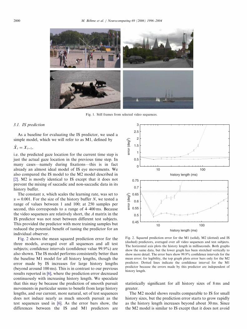
Fig. 1. Still frames from selected video sequences.
0
0.5
1
1.5
2
2.5
3
10 100
erro
r (d
eg2 )
history length (ms)
0.45
0.5
0.55
0.6
0.65
0.7
0.75
10 100
erro
r (d
eg2 )
history length (ms)
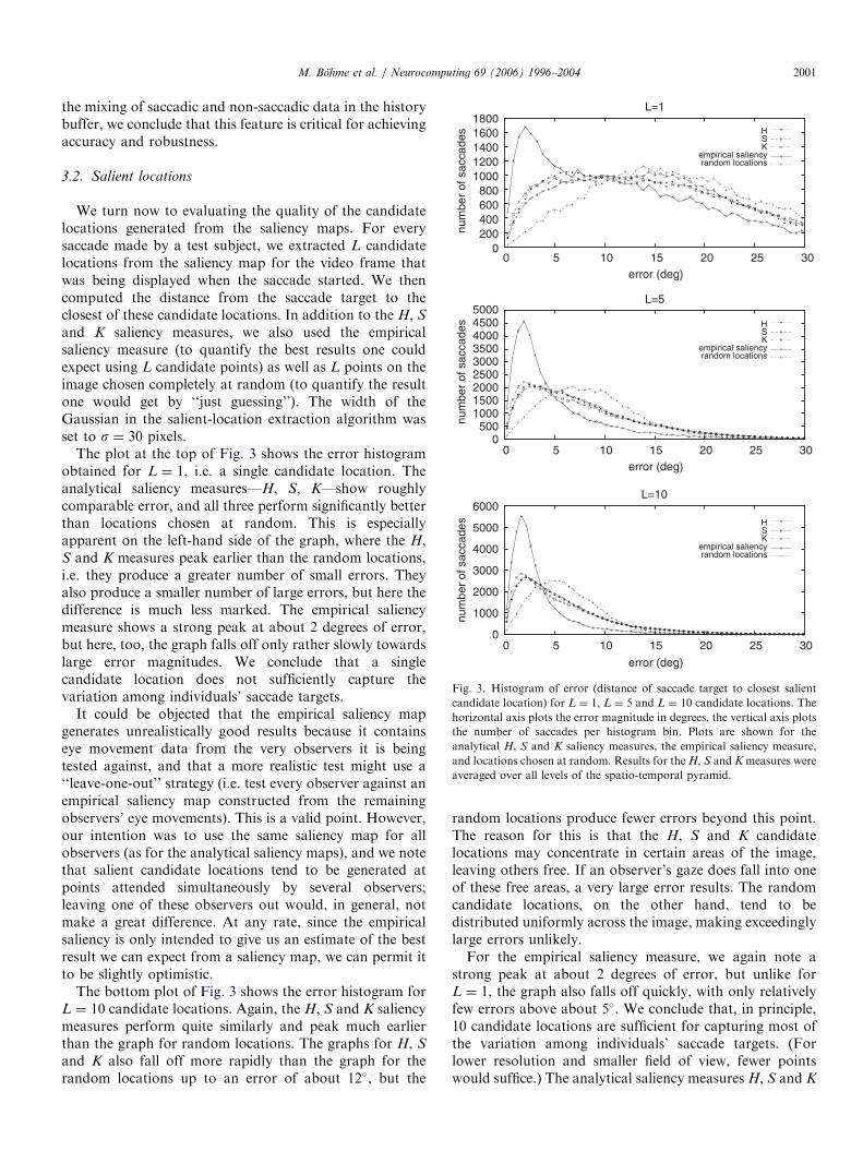
Fig. 2. Squared prediction error for the M1 (solid), M2 (dotted) and IS
(dashed) predictors, averaged over all video sequences and test subjects.
The horizontal axis plots the history length in milliseconds. Both graphs
show the same data, but the lower graph has been stretched vertically to
show more detail. The error bars show 99.9% confidence intervals for the
mean error; for legibility, the top graph plots error bars only for the M2
predictor. Dotted lines indicate the confidence interval for the M1
predictor because the errors made by this predictor are independent of
history length.
M. Bohme et al. / Neurocomputing 69 (2006) 1996–20042000
3.1. IS prediction
As a baseline for evaluating the IS predictor, we used asimple model, which we will refer to as M1, defined by
X t ¼ X t�1,
i.e. the predicted gaze location for the current time step isjust the actual gaze location in the previous time step. Inmany cases—namely during fixations—this is in factalready an almost ideal model of IS eye movements. Wealso compared the IS model to the M2 model described in[2]. M2 is mostly identical to IS except that it does notprevent the mixing of saccadic and non-saccadic data in itshistory buffer.
The constant a, which scales the learning rate, was set toa ¼ 0:001. For the size of the history buffer N, we tested arange of values between 1 and 100; at 250 samples persecond, this corresponds to a range of 4–400ms. Becausethe video sequences are relatively short, the A matrix in theIS predictor was not reset between different test subjects.This provided the predictor with more training samples butreduced the potential benefit of tuning the predictor for anindividual observer.
Fig. 2 shows the mean squared prediction error for thethree models, averaged over all sequences and all testsubjects; confidence intervals (confidence value 99.9%) arealso shown. The IS model performs consistently better thanthe baseline M1 model for all history lengths, though theerror made by IS increases for large history lengths(beyond around 100ms). This is in contrast to our previousresults reported in [6], where the prediction error decreasedcontinuously with increasing history length. We speculatethat this may be because the prediction of smooth pursuitmovements in particular seems to benefit from large historylengths, and our current, more natural, set of test sequencesdoes not induce nearly as much smooth pursuit as thetest sequences used in [6]. As the error bars show, thedifferences between the IS and M1 predictors are
statistically significant for all history sizes of 8ms andgreater.The M2 model shows results comparable to IS for small
history sizes, but the prediction error starts to grow rapidlyas the history length increases beyond about 30ms. Sincethe M2 model is similar to IS except that it does not avoid
ARTICLE IN PRESS
0 200 400 600 800
1000 1200 1400 1600 1800
0 5 10 15 20 25 30
num
ber
of s
acca
des
error (deg)
L=1
HSK
empirical saliencyrandom locations
HSK
empirical saliencyrandom locations
HSK
empirical saliencyrandom locations
0 500
1000 1500 2000 2500 3000 3500 4000 4500 5000
0 5 10 15 20 25 30nu
mbe
r of
sac
cade
serror (deg)
L=5
0
1000
2000
3000
4000
5000
6000
0 5 10 15 20 25 30
num
ber
of s
acca
des
error (deg)
L=10
Fig. 3. Histogram of error (distance of saccade target to closest salient
candidate location) for L ¼ 1, L ¼ 5 and L ¼ 10 candidate locations. The
horizontal axis plots the error magnitude in degrees, the vertical axis plots
the number of saccades per histogram bin. Plots are shown for the
analytical H, S and K saliency measures, the empirical saliency measure,
and locations chosen at random. Results for the H, S and K measures were
averaged over all levels of the spatio-temporal pyramid.
M. Bohme et al. / Neurocomputing 69 (2006) 1996–2004 2001
the mixing of saccadic and non-saccadic data in the historybuffer, we conclude that this feature is critical for achievingaccuracy and robustness.
3.2. Salient locations
We turn now to evaluating the quality of the candidatelocations generated from the saliency maps. For everysaccade made by a test subject, we extracted L candidatelocations from the saliency map for the video frame thatwas being displayed when the saccade started. We thencomputed the distance from the saccade target to theclosest of these candidate locations. In addition to the H, S
and K saliency measures, we also used the empiricalsaliency measure (to quantify the best results one couldexpect using L candidate points) as well as L points on theimage chosen completely at random (to quantify the resultone would get by ‘‘just guessing’’). The width of theGaussian in the salient-location extraction algorithm wasset to s ¼ 30 pixels.
The plot at the top of Fig. 3 shows the error histogramobtained for L ¼ 1, i.e. a single candidate location. Theanalytical saliency measures—H, S, K—show roughlycomparable error, and all three perform significantly betterthan locations chosen at random. This is especiallyapparent on the left-hand side of the graph, where the H,S and K measures peak earlier than the random locations,i.e. they produce a greater number of small errors. Theyalso produce a smaller number of large errors, but here thedifference is much less marked. The empirical saliencymeasure shows a strong peak at about 2 degrees of error,but here, too, the graph falls off only rather slowly towardslarge error magnitudes. We conclude that a singlecandidate location does not sufficiently capture thevariation among individuals’ saccade targets.
It could be objected that the empirical saliency mapgenerates unrealistically good results because it containseye movement data from the very observers it is beingtested against, and that a more realistic test might use a‘‘leave-one-out’’ strategy (i.e. test every observer against anempirical saliency map constructed from the remainingobservers’ eye movements). This is a valid point. However,our intention was to use the same saliency map for allobservers (as for the analytical saliency maps), and we notethat salient candidate locations tend to be generated atpoints attended simultaneously by several observers;leaving one of these observers out would, in general, notmake a great difference. At any rate, since the empiricalsaliency is only intended to give us an estimate of the bestresult we can expect from a saliency map, we can permit itto be slightly optimistic.
The bottom plot of Fig. 3 shows the error histogram forL ¼ 10 candidate locations. Again, the H, S and K saliencymeasures perform quite similarly and peak much earlierthan the graph for random locations. The graphs for H, S
and K also fall off more rapidly than the graph for therandom locations up to an error of about 12�, but the
random locations produce fewer errors beyond this point.The reason for this is that the H, S and K candidatelocations may concentrate in certain areas of the image,leaving others free. If an observer’s gaze does fall into oneof these free areas, a very large error results. The randomcandidate locations, on the other hand, tend to bedistributed uniformly across the image, making exceedinglylarge errors unlikely.For the empirical saliency measure, we again note a
strong peak at about 2 degrees of error, but unlike forL ¼ 1, the graph also falls off quickly, with only relativelyfew errors above about 5�. We conclude that, in principle,10 candidate locations are sufficient for capturing most ofthe variation among individuals’ saccade targets. (Forlower resolution and smaller field of view, fewer pointswould suffice.) The analytical saliency measures H, S and K
ARTICLE IN PRESS
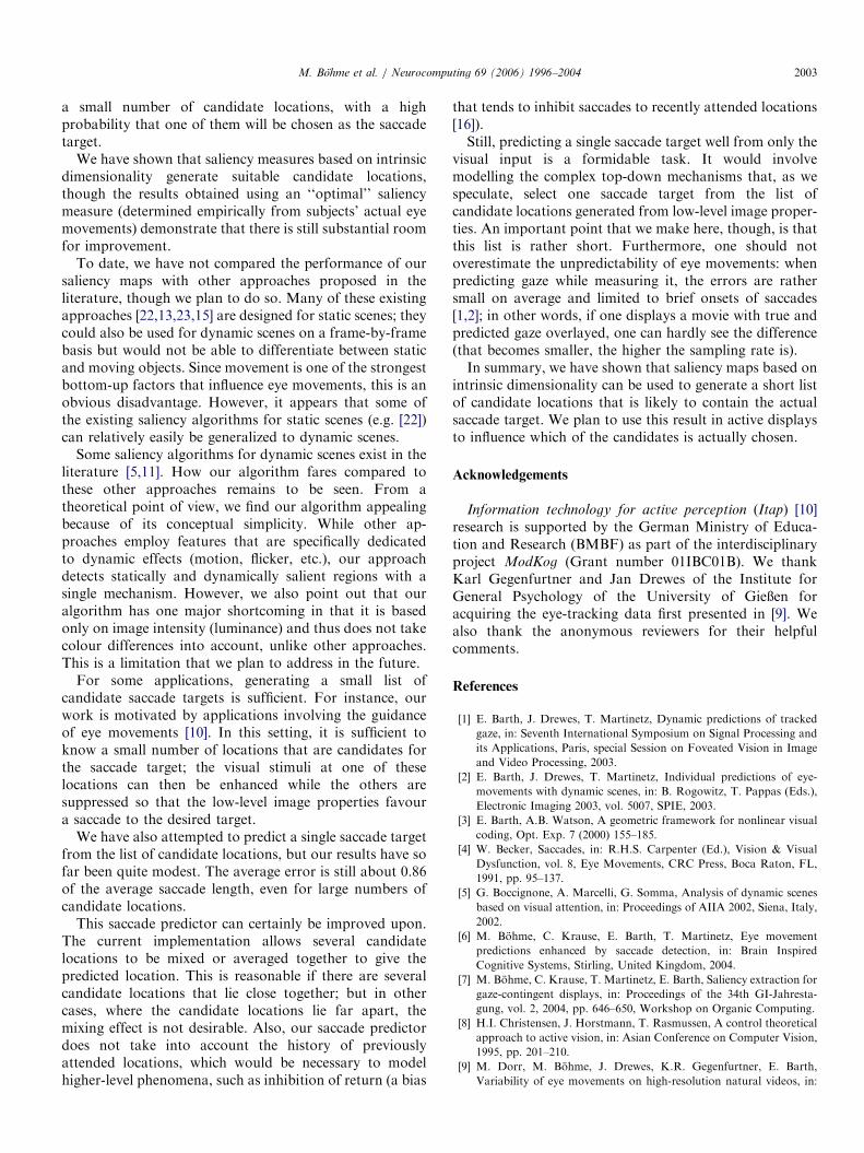
0
0.2
0.4
0.6
0.8
1
1.2
1.4
0 5 10 15 20 25 30
rela
tive
erro
r
number of candidate locations (L)
Fig. 4. Ratio of the average squared prediction error and average squared
saccade length for the saccade predictor (dotted) and ‘‘ideal’’ predictor
(dashed). The horizontal axis plots L, the number of salient locations per
frame.
M. Bohme et al. / Neurocomputing 69 (2006) 1996–20042002
are still quite far away from the optimum represented bythe empirical saliency measure but nevertheless predictsaccade targets well at least some of the time. Picking awinner among the three measures is difficult. The resultsappear to suggest that K may perform slightly better thanH or S, but the differences are too small to make a definiteassessment. For simpler videos with lower resolution wehad found that the higher the intrinsic dimension, thebetter the prediction [7].
Finally, we turn to the middle plot of Fig. 3, whichshows the error histogram for L ¼ 5 candidate locations. Itpresents an intermediate situation between the two plotsdiscussed so far, but we note that the curves are moresimilar in shape to those for L ¼ 10 than those for L ¼ 1,though they do not fall off quite as quickly. This suggeststhat even five locations may already provide adequatecoverage of the eye movements made by differentindividuals.
3.3. Saccade prediction
Finally, we turn to the results of the saccade predictor,which predicts a single saccade target from a list of salientcandidate locations. As an aid for assessing the results, wecompare this predictor with the following three others. Thefirst simply chooses a random point in the image as thepredicted saccade target (this corresponds to the singlerandom candidate location in the previous section). Thesecond predictor chooses the location with maximumsaliency among the candidate locations. The third, ahypothetical ‘‘ideal’’ predictor, always picks the candidatelocation that is closest to the actual saccade target. Thispredictor thus gives us a bound for the best predictionresult we can expect on the given candidate locations if weassume a predictor that selects one of the locations,without any averaging between locations.
The constant b in the saccade predictor, which scales thelearning rate, was set to b ¼ 0:05. The parameter M, whichcontrols the number of video frames used for prediction,was set to M ¼ 1, as incorporating information fromprevious video frames did not seem to improve the resultsmuch. Again, because the video sequences are relativelyshort, the B matrix in the predictor was not reset betweendifferent test subjects. Salient candidate locations weregenerated using the K saliency measure evaluated on thesecond level of the spatio-temporal pyramid, whichperformed slightly better than the other levels.
Fig. 4 shows the performance of the predictor forvarying numbers of candidate locations L, plotted on thehorizontal axis. The vertical axis plots the average squaredprediction error relative to the average squared saccadelength. A ratio of less than 1 means that, on average, thepredictions moved in the right direction relative to thestarting point of the saccade. Results were averaged overall video sequences and all test subjects.
For L ¼ 3 and above, the saccade predictor achieves arelative error of less than 1, showing that, on average, the
prediction moved in the right direction relative to thesaccade starting point. The error decreases with increasingL, though beyond about L ¼ 10 the improvement is small.The relative errors achieved by the ‘‘ideal’’ predictor
start out quite large for small L; initially, they aresubstantially larger than the error for the saccadepredictor. This is explained by the fact that the saccadepredictor makes its prediction relative to the starting pointof the saccade; by limiting the size of this step, the saccadepredictor can limit the size of the error relative to the totalsaccade length. The ‘‘ideal’’ predictor, on the other hand,only has the option of choosing one of the candidatelocations; if all candidate locations are relatively far fromthe actual saccade target, the error made by the predictorwill be relatively large.For increasing L, the error for the ‘‘ideal’’ predictor
decreases continuously, reaching about 0.2 for L ¼ 30candidate locations. This shows the potential for improve-ment that exists with the given saliency information.The relative errors for the random and ‘‘maximum
saliency’’ predictors are constant for all L: 4.51 for therandom predictor and 3.49 for the ‘‘maximum saliency’’predictor. (These values were not shown in the plot becausethey are rather large and would compress the scale of thevertical axis too much.) This underlines the result from theprevious section: a single salient candidate location doesnot capture the variance among individuals well andperforms only slightly better than a location chosen atrandom.
4. Discussion and outlook
The question of just how eye movements are triggeredand controlled is far from being solved. Consequently, theproblem of predicting eye movements remains a difficultone. Our results for the empirical saliency measure showthat predicting the target of a saccade accurately from asaliency map alone is not possible. This is to be expected,given the influence of top-down attentional mechanisms—which are not based primarily on low-level image proper-ties—on the scan-path. However, it seems feasible to select
ARTICLE IN PRESSM. Bohme et al. / Neurocomputing 69 (2006) 1996–2004 2003
a small number of candidate locations, with a highprobability that one of them will be chosen as the saccadetarget.
We have shown that saliency measures based on intrinsicdimensionality generate suitable candidate locations,though the results obtained using an ‘‘optimal’’ saliencymeasure (determined empirically from subjects’ actual eyemovements) demonstrate that there is still substantial roomfor improvement.
To date, we have not compared the performance of oursaliency maps with other approaches proposed in theliterature, though we plan to do so. Many of these existingapproaches [22,13,23,15] are designed for static scenes; theycould also be used for dynamic scenes on a frame-by-framebasis but would not be able to differentiate between staticand moving objects. Since movement is one of the strongestbottom-up factors that influence eye movements, this is anobvious disadvantage. However, it appears that some ofthe existing saliency algorithms for static scenes (e.g. [22])can relatively easily be generalized to dynamic scenes.
Some saliency algorithms for dynamic scenes exist in theliterature [5,11]. How our algorithm fares compared tothese other approaches remains to be seen. From atheoretical point of view, we find our algorithm appealingbecause of its conceptual simplicity. While other ap-proaches employ features that are specifically dedicatedto dynamic effects (motion, flicker, etc.), our approachdetects statically and dynamically salient regions with asingle mechanism. However, we also point out that ouralgorithm has one major shortcoming in that it is basedonly on image intensity (luminance) and thus does not takecolour differences into account, unlike other approaches.This is a limitation that we plan to address in the future.
For some applications, generating a small list ofcandidate saccade targets is sufficient. For instance, ourwork is motivated by applications involving the guidanceof eye movements [10]. In this setting, it is sufficient toknow a small number of locations that are candidates forthe saccade target; the visual stimuli at one of theselocations can then be enhanced while the others aresuppressed so that the low-level image properties favoura saccade to the desired target.
We have also attempted to predict a single saccade targetfrom the list of candidate locations, but our results have sofar been quite modest. The average error is still about 0.86of the average saccade length, even for large numbers ofcandidate locations.
This saccade predictor can certainly be improved upon.The current implementation allows several candidatelocations to be mixed or averaged together to give thepredicted location. This is reasonable if there are severalcandidate locations that lie close together; but in othercases, where the candidate locations lie far apart, themixing effect is not desirable. Also, our saccade predictordoes not take into account the history of previouslyattended locations, which would be necessary to modelhigher-level phenomena, such as inhibition of return (a bias
that tends to inhibit saccades to recently attended locations[16]).Still, predicting a single saccade target well from only the
visual input is a formidable task. It would involvemodelling the complex top-down mechanisms that, as wespeculate, select one saccade target from the list ofcandidate locations generated from low-level image proper-ties. An important point that we make here, though, is thatthis list is rather short. Furthermore, one should notoverestimate the unpredictability of eye movements: whenpredicting gaze while measuring it, the errors are rathersmall on average and limited to brief onsets of saccades[1,2]; in other words, if one displays a movie with true andpredicted gaze overlayed, one can hardly see the difference(that becomes smaller, the higher the sampling rate is).In summary, we have shown that saliency maps based on
intrinsic dimensionality can be used to generate a short listof candidate locations that is likely to contain the actualsaccade target. We plan to use this result in active displaysto influence which of the candidates is actually chosen.
Acknowledgements
Information technology for active perception (Itap) [10]research is supported by the German Ministry of Educa-tion and Research (BMBF) as part of the interdisciplinaryproject ModKog (Grant number 01IBC01B). We thankKarl Gegenfurtner and Jan Drewes of the Institute forGeneral Psychology of the University of GieXen foracquiring the eye-tracking data first presented in [9]. Wealso thank the anonymous reviewers for their helpfulcomments.
References
[1] E. Barth, J. Drewes, T. Martinetz, Dynamic predictions of tracked
gaze, in: Seventh International Symposium on Signal Processing and
its Applications, Paris, special Session on Foveated Vision in Image
and Video Processing, 2003.
[2] E. Barth, J. Drewes, T. Martinetz, Individual predictions of eye-
movements with dynamic scenes, in: B. Rogowitz, T. Pappas (Eds.),
Electronic Imaging 2003, vol. 5007, SPIE, 2003.
[3] E. Barth, A.B. Watson, A geometric framework for nonlinear visual
coding, Opt. Exp. 7 (2000) 155–185.
[4] W. Becker, Saccades, in: R.H.S. Carpenter (Ed.), Vision & Visual
Dysfunction, vol. 8, Eye Movements, CRC Press, Boca Raton, FL,
1991, pp. 95–137.
[5] G. Boccignone, A. Marcelli, G. Somma, Analysis of dynamic scenes
based on visual attention, in: Proceedings of AIIA 2002, Siena, Italy,
2002.
[6] M. Bohme, C. Krause, E. Barth, T. Martinetz, Eye movement
predictions enhanced by saccade detection, in: Brain Inspired
Cognitive Systems, Stirling, United Kingdom, 2004.
[7] M. Bohme, C. Krause, T. Martinetz, E. Barth, Saliency extraction for
gaze-contingent displays, in: Proceedings of the 34th GI-Jahresta-
gung, vol. 2, 2004, pp. 646–650, Workshop on Organic Computing.
[8] H.I. Christensen, J. Horstmann, T. Rasmussen, A control theoretical
approach to active vision, in: Asian Conference on Computer Vision,
1995, pp. 201–210.
[9] M. Dorr, M. Bohme, J. Drewes, K.R. Gegenfurtner, E. Barth,
Variability of eye movements on high-resolution natural videos, in:
ARTICLE IN PRESSM. Bohme et al. / Neurocompu2004
H.H. Bulthoff, H.A. Mallot, R. Ulrich, F.A. Wichmann (Eds.),
Proceedings of the Eighth Tubinger Perception Conference, 2005,
p. 162.
[10] Information technology for active perception, 2002, URL: hhttp://
www.inb.uni-luebeck.de/Itap/i.
[11] L. Itti, Quantifying the contribution of low-level saliency to human
eye movements in dynamic scenes, Visual Cognit. 12 (6) (2005)
1093–1123.
[12] L. Itti, Models of bottom-up attention and saliency, in: L. Itti, G.
Rees, J.K. Tsotsos (Eds.), Neurobiology of Attention, Elsevier, San
Diego, CA, 2005, pp. 576–582.
[13] L. Itti, C. Koch, Computational modelling of visual attention, Nature
Rev. Neurosci. 2 (3) (2001) 194–203.
[14] B. Jaehne, H. HauXecker, P. GeiXler (Eds.), Handbook of Computer
Vision and Applications, Academic Press, New York, 1999.
[15] T. Kadir, A. Zisserman, M. Brady, An affine invariant salient region
detector, in: Eighth European Conference on Computer Vision, vol.
1, Springer, Berlin, 2004, pp. 257–269.
[16] R.M. Klein, Inhibition of return, Trends Cognit. Sci. 4 (2000)
138–147.
[17] R.J. Leigh, D.S. Zee (Eds.), The Neurology of Eye Movements,
Oxford University Press, Oxford, 1999.
[18] D.M. MacKay, Behind the Eye, Basil Blackwell, Oxford, 1991.
[19] C. Mota, E. Barth, On the uniqueness of curvature features, in: G.
Baratoff, H. Neumann (Eds.), Dynamische Perzeption, Proceedings
in Artificial Intelligence, vol. 9, Infix Verlag, Koln, 2000, pp. 175–178.
[20] D. Noton, L. Stark, Eye movements and visual perception, Sci. Am.
224 (6) (1971) 34–43.
[21] J.K. O’ Regan, A. Noe, A sensorimotor account of vision and visual
consciousness, Behav. Brain Sci. 24 (5) (2001) 939–1011.
[22] C.M. Privitera, L.W. Stark, Algorithms for defining visual regions-of-
interest: Comparison with eye fixations, IEEE Trans. Pattern Anal.
Mach. Intell. 22 (9) (2000) 970–982.
[23] F. Stentiford, An estimator for visual attention through competitive
novelty with application to image compression, in: Picture Coding
Symposium, Seoul, Korea, 2001, pp. 101–104.
[24] C. Zetzsche, E. Barth, Fundamental limits of linear filters in the
visual processing of two-dimensional signals, Vision Res. 30 (1990)
1111–1117.
[25] C. Zetzsche, K. Schill, H. Deubel, G. Krieger, E. Umkehrer, S.
Beinlich, Investigation of a sensorimotor system for saccadic scene
analysis: an integrated approach, in: R. Pfeifer, B. Blumberg, J.-A.
Meyer, S.W. Wilson (Eds.), From Animals to Animats 5: Proceedings
of the Fifth International Conference on Simulation of Adaptive
Behavior, vol. 5, MIT Press, Cambridge, 1998, pp. 120–126.
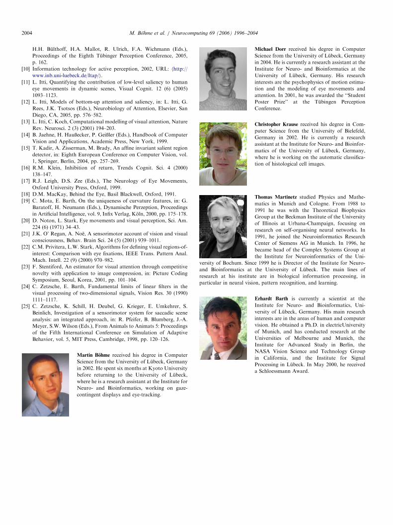
Martin Bohme received his degree in Computer
Science from the University of Lubeck, Germany
in 2002. He spent six months at Kyoto University
before returning to the University of Lubeck,
where he is a research assistant at the Institute for
Neuro- and Bioinformatics, working on gaze-
contingent displays and eye-tracking.
Michael Dorr received his degree in Computer
Science from the University of Lubeck, Germany
in 2004. He is currently a research assistant at the
Institute for Neuro- and Bioinformatics at the
University of Lubeck, Germany. His research
interests are the psychophysics of motion estima-
tion and the modeling of eye movements and
attention. In 2001, he was awarded the ‘‘Student
Poster Prize’’ at the Tubingen Perception
Conference.
ting 69 (2006) 1996–2004
Christopher Krause received his degree in Com-
puter Science from the University of Bielefeld,
Germany in 2002. He is currently a research
assistant at the Institute for Neuro- and Bioinfor-
matics of the University of Lubeck, Germany,
where he is working on the automatic classifica-
tion of histological cell images.
Thomas Martinetz studied Physics and Mathe-
matics in Munich and Cologne. From 1988 to
1991 he was with the Theoretical Biophysics
Group at the Beckman Institute of the University
of Illinois at Urbana-Champaign, focusing on
research on self-organising neural networks. In
1991, he joined the Neuroinformatics Research
Center of Siemens AG in Munich. In 1996, he
became head of the Complex Systems Group at
the Institute for Neuroinformatics of the Uni-
versity of Bochum. Since 1999 he is Director of the Institute for Neuro-
and Bioinformatics at the University of Lubeck. The main lines of
research at his institute are in biological information processing, in
particular in neural vision, pattern recognition, and learning.
Erhardt Barth is currently a scientist at the
Institute for Neuro- and Bioinformatics, Uni-
versity of Lubeck, Germany. His main research
interests are in the areas of human and computer
vision. He obtained a Ph.D. in electricUniversity
of Munich, and has conducted research at the
Universities of Melbourne and Munich, the
Institute for Advanced Study in Berlin, the
NASA Vision Science and Technology Group
in California, and the Institute for Signal
Processing in Lubeck. In May 2000, he received
a Schloessmann Award.