v ,+- P J&N@t. qy

&?@dq ,#*J / Final Technical Report

October 1, 1986 t o September 30, 1987 l'/J -t2~~''''''

ey7&0?

y7 %: Implementation and Validation of a Wake Model fo r Low-Speed

Forward Flight

Narayanan M . Komerath Olivier A. Schreiber (Principal Investigator) (Graduate Research Assistant)

School of Aerospace Engineering Georgia Inst i tute of Technology Atlanta, Georgia 30332

Prepared for: Langley Research Center under Grant NAG-1-693 NASA Technical Officer

Mr. John D . Berry LSAD M/S 286

GTAER 07-3 September 1987

https://ntrs.nasa.gov/search.jsp?R=19870019081 2018-06-15T07:08:10+00:00Z

Final Technical Report October 1, 1986 t o September 30, 1987

Implementation and Validation of a Wake Model fo r Low-Speed

Forward Flight

Narayanan M . Komerath Olivier A. Schreiber (Principal Investigator) (Graduate Research Assistant)

School of Aerospace Engineering Georgia Institute of Technology Atianta, Georgia 321332

Prepared for : Langley Research Center under Grant NAG-1-693 NASA Technical Officer

Mr. John D . Berry LSAD M/S 286

GTAER 87-3 September 1987

Abs t rac t

This report details the computer implementation and calculations of the induced velocities produced by a wake model consisting of a trailing vortex system defined from a prescribed time averaged down- wash distribution. Induced velocities are computed by approximating each spiral turn by a pair of large straight vortex segments positioned at critical points relative to where the induced velocity is required. A remainder term for the rest of the spiral turn is added. This ap- proach results in decreased computation time compared to classical models where each spiral turn is broken down in small straight vortex segments The model includes features such as harmonic variation of circulation, downwash outside of the blade and/or outside the tip pat.h plane, blade bound vorticity induced velocity with harmonic variation of circulation and time averaging. The influence of various options and parameters on the results are investigated and results are compared to experimental field measurements with which, a reason- able agreement is obtained. The capabilities of the model as well as its extension possibilities are studied. An assessment of the model for possible adptation to interaction problems shows it not to be suitable for this purpose. However, further features like a shed vortex sys- tem, an inboard trailing wake system, close blade vortex interaction and lifting surface effects can be added to it. The performance of the model in predicting the recently-acquired NASA Langley Inflow data base for a four-bladed rotor is compared to that. of the S c d y Free Wake code. a well-established program which requires much greater computational resources. It is found that the two codes predict the experimental data with essentially the same accuracy, and show the same trends. The model is an efficient and flexible tool t o obtain a de- scription of a rotor’s induced downwash field in a workstation-type of environment with accuracies comparable to those obtained by codes requiring an order of magnitude more of computer resources.

GO N TEN T S 1

I

Contents 1 Nomenclature 5

2 Introduction 9

3 General description of the wake model 11

4 Tip vortex geometry 12

5 Computation of induced velocities 16 5.1 Pair of vortex segments . . . . . . . . . . . . . . . . . . . . 16 5.2 Remainder t. ern1 . . . . . . . . . . . . . . . . . . . . . . . . 20 5.3 Blade bound vorticity . . . . . . . . . . . . . . . . . . . . . 21 r).r Pidid iiveiiiging of d f i W i i W i d i . . . . . . . . . . . . . . . . . LO C A 0 0

6 Positioning of the vortex elements 25

7 Development of the code 26 7.1 Structure of the code . . . . . . . . . . . . . . . . . . . . . . 26 7.2 FORTRAN implementation . . . . . . . . . . . . . . . . . . 27 7.3 Graphics implementation . . . . . . . . . . . . . . . . . . . 27

8 Computations 28 8.1 Input. Data . . . . . . . . . . . . . . . . . . . . . . . . . . . 28 8.2 First module visualization . . . . . . . . . . . . . . . . . . . 29 8.3 Second module visualization . . . . . . . . . . . . . . . . . . 29 8.4 Induced downwash computations . . . . . . . . . . . . . . . 29

8.4.1 Three dimensional plots . . . . . . . . . . . . . . . . 30 8.4.2 Contour plots, influence of input. parameters . . . . 31 8.4.3 Final results . . . . . . . . . . . . . . . . . . . . . . 33

8.5 Computation time . . . . . . . . . . . . . . . . . . . . . . . 34 8.6 Comparison with Scully Free-Wake Code . . . . . . . . . . . 34

9 Capabilities of the code 35 9.1 Capabilities . . . . . . . . . . . . . . . . . . . . . . . . . . . 35 9.2 Potential for growth . . . . . . . . . . . . . . . . . . . . . . 35

CONTENTS 2

9.3 Adaptability to interaction problems . . . . . . . . . . . . . 36

10 Conclusions 37

11 Acknowledgements 37

A User’s Manual 39 A. l Introduction. . . . . . . . . . . . . . . . . . . . . . . . . . . 39 A.2 First, iiiodule . . . . . . . . . . . . . . . . . . . . . . . . . . 39 A.3 Second Module . . . . . . . . . . . . . . . . . . . . . . . . . 40 A.4 Third Module . . . . . . . . . . . . . . . . . . . . . . . . . . 41

A.4.1 Test -Velocity . . . . . . . . . . . . . . . . . . . . . 42 A.4.2 Frontal.. . . . . . . . . . . . . . . . . . . . . . . . 43

LIST OF FIGURES 3

List of Figures 1 2 3 4 5 6 7 8 9 10 11 12 13 14 15 16 17 18 19 20 21 22 23 24 25 26 27 28 29

30

31 32

Induced downwash computation . . . . . . . . . . . . . . . . 9 Trailing vortex system . . . . . . . . . . . . . . . . . . . . . 11 cos$, > 0 . . . . . . . . . . . . . . . . . . . . . . . . . . . . 13 ... $. < 0. .. < -T. ... $. . . . . . . . . . . . . . . . . . . . 14 cos$. < 0. .. > -T. cos$. . . . . . . . . . . . . . . . . . . . 14 Vortex segments . . . . . . . . . . . . . . . . . . . . . . . . 17 Local unit vectors . . . . . . . . . . . . . . . . . . . . . . . 18 Vector decomposition . . . . . . . . . . . . . . . . . . . . . 19 Sign of p B . . . . . . . . . . . . . . . . . . . . . . . . . . . . 21 First module visualisation . . . . . . . . . . . . . . . . . . . 47 Second module visualisation . . . . . . . . . . . . . . . . . . 48 Instantaneous induced velocities (3-D) . . . . . . . . . . . . 49 Induced downwash iieid (3 -0 j . . . . . . . . . . . . . . . . . 50 Instantaneous induced velocities. detailed (3-D) . . . . . . . 51 Instantaneous induced velocities (Contour) . . . . . . . . . 52 Induced downwash field (Contour) . . . . . . . . . . . . . . 53 Radial averaging influence . . . . . . . . . . . . . . . . . . . 54 Number of spiral turns influence (1) . . . . . . . . . . . . . 55 Number of spiral turns influence (5) . . . . . . . . . . . . . 56 Contracted radius size influence . . . . . . . . . . . . . . . . Vortex .... size influence . . . . . . . . . . . . . . . . . . . 58 Freestream inflow component influence . . . . . . . . . . . . Remainder term size influence (small value) . . . . . . . . . Remainder term size influence (large value) . . . . . . . . . 61

57

59 60

Circulation zeroth harmonic component influence (small value) 62 Circulation zeroth harmonic component influence (large value) 63 Circulation first harmonic component influence (longitudinal) 64 Circulation first harmonic component influence (lateral) . . 65 Circulation first harmonic component influence on induced

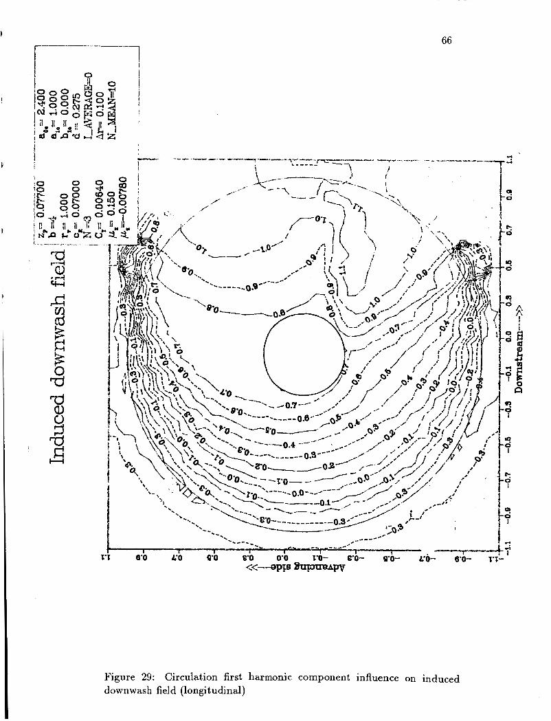
Circulation first harmonic component influence on induced downwash field (longitudinal) . . . . . . . . . . . . . . . . . 66

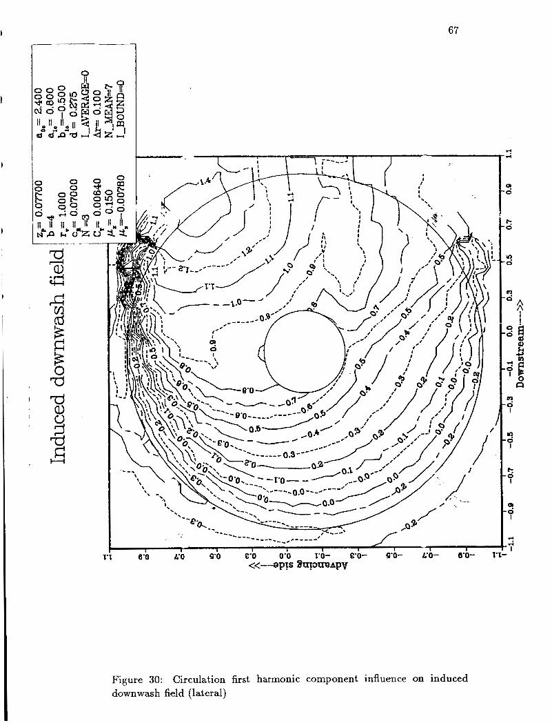
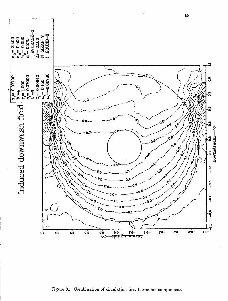
downwash field (lateral) . . . . . . . . . . . . . . . . . . . . 67 Combination of circulation first harmonic components . . . 68 Blade bound circulation influence . . . . . . . . . . . . . . . 69

LIST OF FIGURES

33 34 35 36 37 38 39 40 41 42 43 44 45 46 4 i 48 49 50 51

52

53

54

55

56

57

58

Final choice of circulation first harmonic components . . . . Experiment a1 results . . . . . . . . . . . . . . . . . . . . . . Comparison computation-experiment at 0. degrees azimuth Comparison computation-experiment at 30. degrees azimuth Comparison computation-experiment at 60. degrees azimuth Comparison computation-experiment at, 90. degrees azimuth Comparison computation-experiment, at 120. degrees azimuth Comparison computation-experiment, at 150. degrees azimuth Comparison computation-experiment at 180. degrees azimuth Comparison computation-experiment. at 210. degrees azimuth Comparison computation-experiment. at. 240. degrees azimuth Comparison computation-experiment at 270. degrees azimuth Comparison computation-experiment. at, 300. degrees azimuth

Comparison Free-Wake and experiment at 0. degrees azimut,h Comparison Free-Wake and experiment, at, 30. degrees azimuth Comparison Free-Wake and experiment. at 60. degrees azimuth Comparison Free-Wake and experiment, at. 90. degrees azimuth Comparison Free-Wake and experiment at 120. degrees az- imuth . . . . . . . . . . . . . . . . . . . . . . . . . . . . . . Comparison Free-Wake and experiment, at, 150. degrees az- imuth . . . . . . . . . . . , . . . . . . . . . . . . . . . . . . Comparison Free-Wake and experiment- at, 180. degrees az- imuth . . . . . . . . . . . . . . . . . . . . . . . . . . . . . . Comparison Free-Wake and experiment. at 210. degrees az- imuth . . . . . . . . . . . . . . . . . . . . . . . . . . . . . . Comparison Free-Wake and experiment at 240. degrees az- imuth . . . . . . . . . . . . . . . . . . . . . . . . . . . . . . Comparison Free-Wake and experiment at, 270. degrees az- imuth . . . . . . . . . . . . . . . . . . . . . . . . . . . . . . Comparison Free-Wake and experiment, at 300. degrees az- imuth . . . . . . . . . . . . . . . . . . . . . . . . . . . . . . Comparison Free-Wake and experiment. at 330. degrees az- imuth . . . . . . . . . . . . . . . . . . . . . . . . . . . . . .

ccrr,n1r;enn r-'-"' rnmniit -"-".VI. ~ + ; o n - e ~ p e ~ ~ e ~ f . , z!, 330. C I e m c n n c u . I L I ' . A U I L Qv;m**th

4

70 71 7'2 73 74 75 76

78 79 80 81 82 83 84 85 86 8'7

88

89

90

91

92

93

94

95

CF

( 1

5

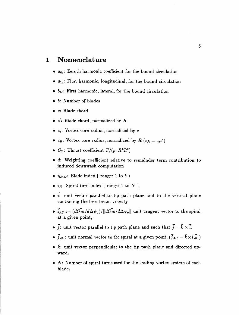
1 Nornenclat ure 0 ao,: Zeroth harmonic coefficient for the bound circulation

0 al,: First harmonic, longitudinal, for the bound circulation

0 bl,: First harmonic, lateral, for the bound circulation

0 b: Number of blades

0 c: Blade chord

0 c': Blade chord, normalized by R

e d: Weighting coefficient relative to remainder term contribution to induced downwash computation

0 &lade: Blade index ( range: 1 to b )

0 iN: Spiral turn index ( range: 1 to N )

0 2 : unit vector parallel to tip path plane and to the vertical plane f

containing the freestream velocity

0 ~ A C := ( d O ~ / d A ~ , ) / l l d O t m / d A ~ , l l unit tangent vector to the spiral at a given point,

0 7: unit vector parallel to tip path plane and such that j'= 0 J A C : unit normal vector to the spiral at a given point, (TAC = k x Z A C )

0 k: unit vector perpendicular to the tip path plane and directed up-

x r. + + f

+

ward.

0 N : Number of spiral turns used for the trailing vortex system of each blade.

1 NOMENCLATURE 6

0 N M E A N : Number of divisions of one sector used to average the in- duced downwash over azimuth. (One sector is the angle between two consecutive blades, i.e. (27r/b)

0 P: Point where the induced velocity is being computed - 7 +

0 p g : projection of vector P B on ;Ac ( p B = P B . J A ~ )

0 rp: Radial coordinate of point P, where the induced velocity is being computed normalized by R

0 r,: Contracted radius, normalized by R

0 R: Rotor radius

0 72: Algebraic curvature radius of projected spiral in tip path plane

0 2': Rotor thrust

0 o: Induced velocity (positive up)

0 V: Free stream velocity

0 z, y, z : Coordinates of a point in the z, ;, vector base.

0 z p : z ordinate difference between point P and tip path plane, nor- malized by R, (Positive above tip path plane).

0 zpg: z ordinate difference between point P and point B, normalized + +

by R ( t p ~ = k .PB/R = zg - ~p = Z, - ~ p )

0 a: Angle of attack, of rotor tip path plane (negative in forward flight)

0 a: Radial abscissa integration variable

0 p: Angle between vortex segment and blade of reference ( p = @,-+p)

0 p: Integration variable

0 A$,: age of a vortex line point.

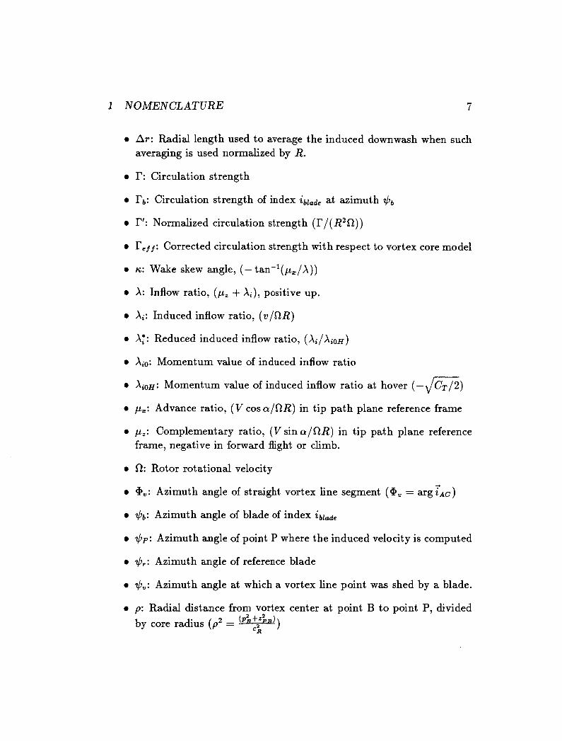
1 NOMENCLATURE 7

0 AT: Radial length used to average the induced downwash when such averaging is used normalized by R.

0 I?: Circulation strength

0 r b : Circulation strength of index

0 I”: Normalized circulation strength (r/( R2s1))

0 reff: Corrected circulation strength with respect to vortex core model

0 K: Wake skew angle, (- tan-’(p,/A))

0 A: Inflow ratio, (pz + Ai), positive up.

0 Ai: Induced inflow ratio, (v /RR)

0 At: Reduced induced inflow ratio, (A;/A~OH)

0 Aio: Momentum value of induced inflow ratio

at azimuth $b

0 Aio*: Momentum value of induced inflow ratio at hover (-dm) 0 pz: Advance ratio, (V cos a/RR) in tip path plane reference frame

0 pz: Complementary ratio, (V sin a / Q R ) in tip path plane reference frame, negative in forward flight or climb.

0 s1: Rotor rotational velocity

0 !Du: Azimuth angle of straight vortex line segment (!Du = argz+&)

0 $b: Azimuth angle of blade of index &lade

0 $ p : Azimuth angle of point P where the induced velocity is computed

0 $?: Azimuth angle of reference blade

0 &,: Azimuth angle at which a vortex line point was shed by a blade.

0 p: Radial distance from vortex center at point B to point P, divided

9 2 - (P’,+.’,, by core radius ( p - C’R

1 NOMENCLATURE

0 p: Air density, where appropriate

0 Q: Rotor solidity, (bc/?rR)

8

9

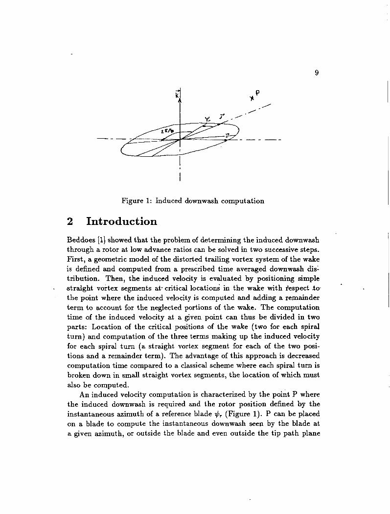
Figure 1: Induced downwash computation

2 Introduction Beddoes [l] showed that the problem of determining the induced downwash through a rotor at low advance ratios can be solved in two successive steps. First, a geometric model of the distorted trailing vortex system of the wake is defined and computed from a prescribed time averaged downwash disl tribution. Then, the induced velocity is evaluated by positioning simple straight vortex segments at- critical locations in the wake with fespect io . the point where the induced velocity is computed and adding a remainder term to account for the neglected portions of the wake. The computation time of the induced velocity at a given point can thus be divided in two parts: Location of the critical positions of the wake (two for each spiral turn) and computation of the three terms making up the induced velocity for each spiral turn (a straight vortex segment for each of the two posi- tions and a remainder term). The advantage of this approach is decreased computation time compared to a classical scheme where each spiral turn is broken down in small straight vortex segments, the location of which must also be computed.

An induced velocity computation is characterized by the point P where the induced downwash is required and the rotor position defined by the instantaneous azimuth of a reference blade $r (Figure 1). P can be placed on a blade to compute the instantaneous downwash seen by the blade at a given azimuth, or outside the blade and even outside the tip path plane

-

11

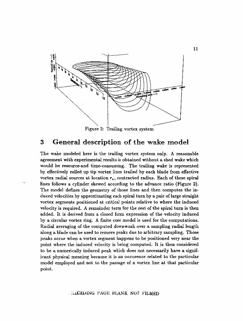
Figure 2: Trailing vortex system

3 Generd descriptioll of the wake mde l The wake modeled here is the trailing vortex system only. A reasonable agreement with experimental results is obtained without a shed wake which would be resource-and time-consuming. The trailing wake is represented by effectively rolled up tip vortex lines trailed by each blade from effective vortex radial sources at location ru, contracted radius. Each of these spiral lines foHows a cylinder skewed according to the advance ratio (Figure 2). The model defines the geometry of those lines and then computes the in- duced velocities by approximating each spiral turn by a pair of large straight vortex segments positioned at critical points relative to where the induced velocity is required. A remainder term for the rest of the spiral turn is then added. It is derived from a closed form expression of the velocity induced by a circular vortex ring. A finite core model is used for the computations. Radial averaging of the computed downwash over a sampling radial length along a blade can be used to remove peaks due to arbitrary sampling. Those peaks occur when a vortex segment happens to be positioned very near the point where the induced velocity is being computed. It is then considered to be a numerically induced peak which does not necessarily have a signif- icant physical meaning because it is an occurence related to the particular model employed and not to the passage of a vortex line at that particular point.

:,&EULNC; PAGE BLANK NOT FILMED

12

4 Tip vortex geometry

A prescribed geometry presented in reference [2] is used. The vertical dis- placement of elements of the wake is computed by integration of a pre- scribed time averaged downwash field given in reference [3]. The tip vortex lines are represented parametrically in the tip path plane frame of reference (z, 7, <) moving with the rotor. The parameters are:

1.

2.

3.

ibl& or the index of the blade from which the given vortex line trails ( range: 1 to b )

$t the angular position of the reference rotor blade (&ade = 1) ( range: -

0 to 2n )

A+, the age of a vortex line element. It is defined as the angle by which the rotor has turned since that element was produced. ( range: 0 to 2N7r )

The averaged downwash field, within the disc defined by the contracted radius T, is given by:

xi = xiO(l + E ~ ' - ~ l ~ ' 3 1 ) (4)

where primed values are normalized by T, and E = In/. Outside the disc, and dowstream of the tip path plane center, the averaged downwash field is given by:

xi = 2xi0(i - ~ 1 ~ 1 3 1 ) ( 5 )

4 TIP VORTEX GEOMETRY 13

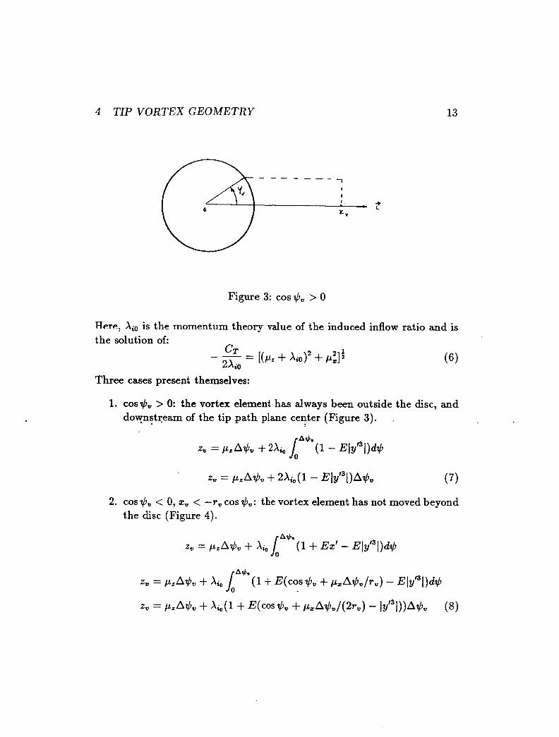
Figure 3: cos+, > 0

Here; Xi, is the momentum theory value of the induced inflow ratio and is the solution of

- [(pz + x;o)2 + P$ (6) CT

2&0

---

Three cases present themselves:

1. cos+, > 0: the vortex element has always been outside the disc, and downstream of the tip path plane center (Figure 3). .

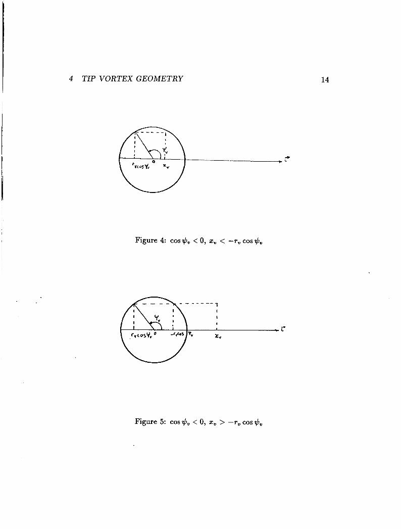
2. cos $, < 0, z, < -T, cos 4,: the vortex element has not moved beyond the disc (Figure 4).

4 TIP VORTEX GEOMETRY 14

Figure 4: cos& < 0, xu < -r, cos $,

1 I

I t I 4 c c xu

Figure 5: cos $,, < 0, x, > -ru cos &,

4 TIP VORTEX GEOMETRY 15

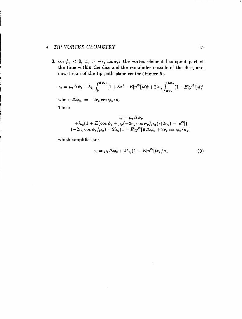
3. cos$, < 0, 2, > -T, cos&: the vortex element has spent part of the time within the disc and the remain.der outside of the disc, and dowstream of the tip path plane center (Figure 5).

where A$ul = -2r, cos t+$,/pz

Thus:

which simplifies to:

5

16

Computation of induced velocities For each spiral turn, the vortex lines trailed by each blade are accounted for in the computation of induced velocity by placing a pair of straight vortex segments at critical locations, and adding a remainder term. In this model, the vortex lines have first harmonic circulation variation with the local azimuth $, at which a particular point was shed. A point belonging to a vortex line will be attributed a circulation strength equal to that of the blade from which the line is trailing at the time when the blade shed that paticular point, that is azimuth $,. The zeroth harmonic component of circulation is related to the thrust coefficient. Since each blade is trail- ing concentrated vortex lines from a single radial station (the contracted radius), then the bound vorticity should be constant along each blade and then, fall off abruptly at the contracted radius. Since no inboard trailing vortex line is included, the bound vorticity should be constant from the center of the rotor to the contracted radius. Thus, the bound vorticity of each blade is modeled as constant circulation straight vortex segments of length equal to the contracted radius.

Reference [l] presents a radially averaged downwash expression. It can be used for the distribution of downwash along a blade to smooth out peaks appearing because of the discrete nature of the sample of points where the induced downwash is computed. Those peaks occur when a vortex segment happens to be positioned very near the point where the induced velocity is being computed. It is then considered to be a numerically induced peak which does not necessarily have a significant physical meaning because it is an occurence related to the particular model employed and not to the passage of a vortex line at that particular point. The averaging length then should be of the order of the definition interval of the sampling.

5.1 Pair of vortex segments For a given point P where the induced velocity is needed, and for each spiral turn of each vortex line, two points B are positioned to support a straight vortex segment of length 2r, and circulation rejj. The segments are horizontal (i.e. oriented parallel to the tip path plane) and each is contained in a vertical plane tangent to the spiral such that the vertical

5 COMPUTATION OF INDUCED VELOCITIES

P h

17

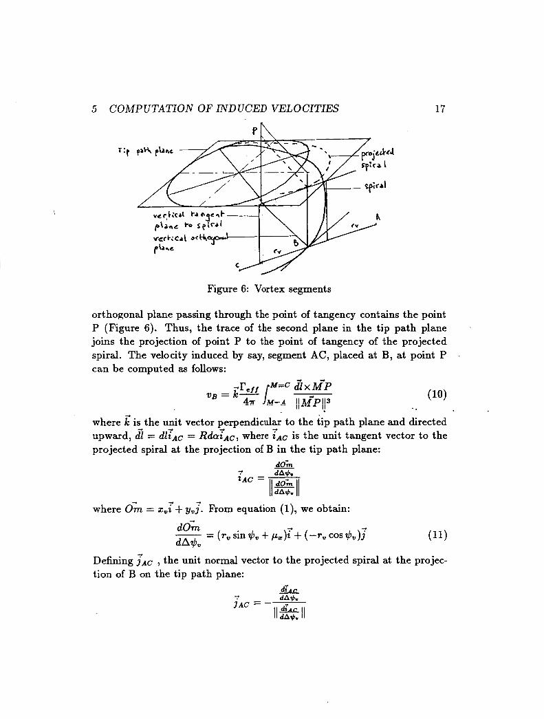
Figure 6: Vortex segments

orthogonal plane passing through the point of tangency contains the point P (Figure 6). Thus, the trace of the second plane in the tip path plane joins the projection of point P to the point of tangency of the projected spiral. The velocity induced by say, segment AC, placed at B, at point P can be computed as follows:

.

where is the unit vector perpendicular to the tip path plane and directed upward, dl = d l z A c = Rdaz~c, where ~ A C is the unit tangent vector to the projected spiral at the projection of B in the tip path plane:

+

+

where Om = zu7+ yvl. From equation (l), we obtain:

Defining T A c , the unit normal vector to the projected spiral at the projec- tion of B on the tip path plane:

5 COMPUTATION OF INDUCED VELOCITIES 18

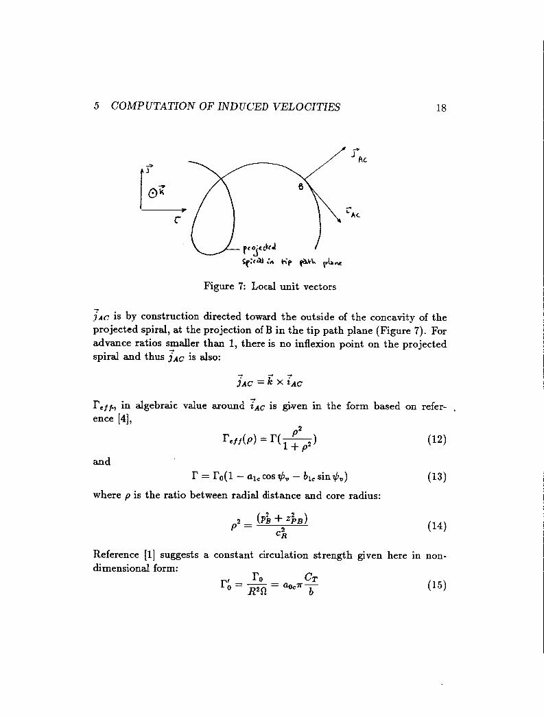
Figure 7: Local unit vectors

j ~ c is by construction directed toward the outside of the concavity of the projected spiral, at the projection of B in the tip path plane (Figure 7). For advance ratios smaller than 1, there is no inflexion point on the projected spiral and thus TAC is also:

f - ? 3AC = k x ZAC

-. reff., in algebraic value around ZAC is given in the form based on refer- . ence [4],

and I’ = ro( 1 - ulc COS & - blc sin $,) (13)

where p is the ratio between radial distance and core radius:

Reference [l] suggests a constant circulation strength given here in non- dimensional form:

r0 CT r; = R2R = Qcxb

5 COMPUTATION OF INDUCED VELOCITIES 19

with tion,

Thus,

P.

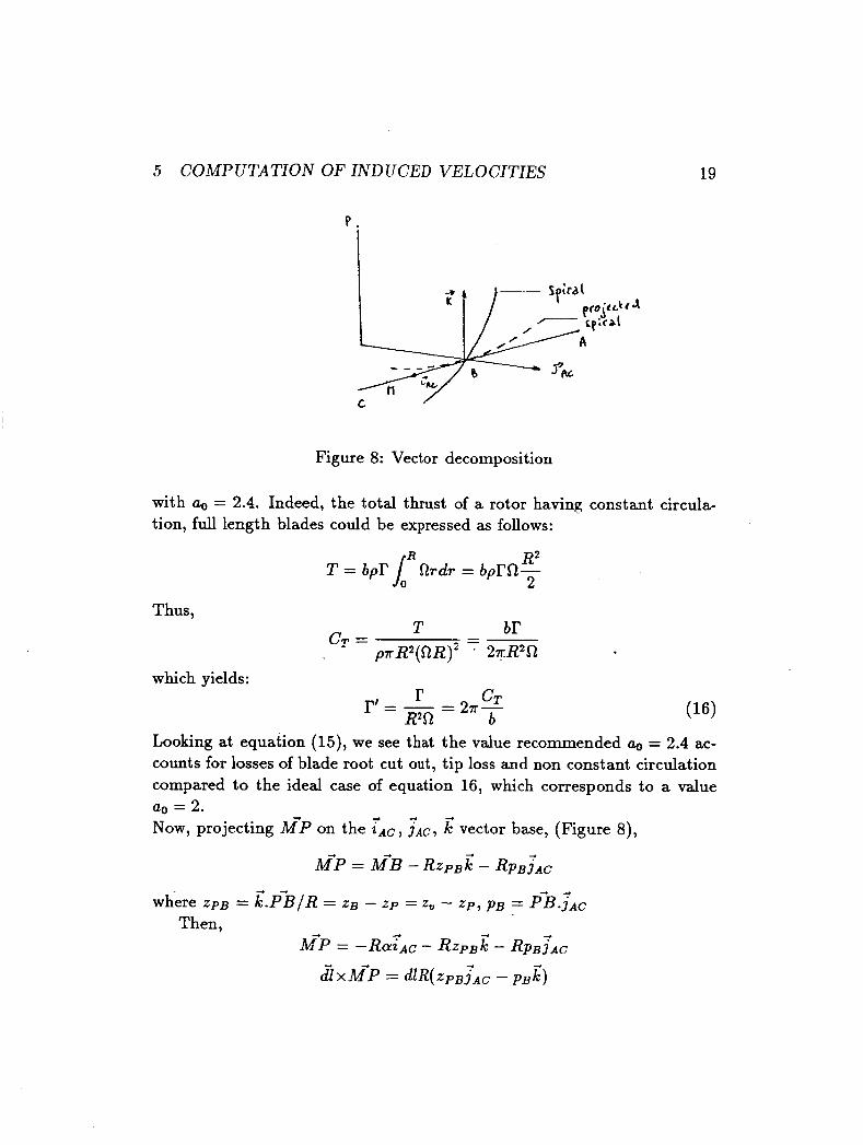
Figure 8: Vector decomposition

Q, = 2.4. Indeed, the total thrust of a rotor having constant circula- full length blades could be expressed as follows:

which yields:

R R2 T = b p r l flrdr = b p r f l - 2

r CT = - R2R = 2?rb

Looking at equation (15), we see that the value recommended Q, = 2.4 ac- counts for losses of blade root cut out, tip loss and non constant circulation compared to the ideal case of equation 16, which corresponds to a value aq-j = 2. Now, projecting M-P on the TAG, ; ~ c , $ vector base, (Figure 8),

-4 4

M P = M B - ~ t ~ ~ $ - ~ p ~ j ' ~ ~ - 4 f - 4

where z p g = k .PB/R = zg - z p = 2, - z p , p g = PB.]Ac

f -4 Then,

hf-p = -RCY~AC - R z p g k - Rpg~Ac -4

XM-P = dlR( zp~TAc - p g I C )

5 COMPUTATION OF INDUCED VELOCITIES 20

+ + * and

k ( d Z x M P ) = -RpBdl = -R2pBda

Also, we have (M-P)’ = (a2 + z i B + &)R2 thus:

Switching to non-dimensional variables with v i = V B / ( R R ) and reff/( R2R), we obtain:

=

Letting P2 = zgB + p i and sinh 8 = ;,

vb = -- r:ffpB tanh(arg sinh( 5)) 2 7 r p P

I &fPB 1 V B = -- 2np2 JW’

Thus, we finally have the expression vb:

5.2 Remainder term The remainder term accounts for the contribution of the remaining por- tion of the spiral turn. Reference 1 provides the following approximate expression.

5 COMPUTATION OF INDUCED VELOCITIES 21

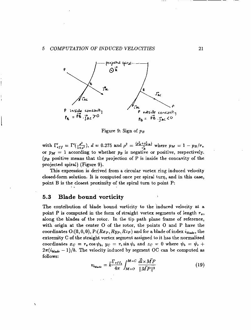
Figure 9: Sign of p~

2 - (P?7+Z2 with Lf = I?(&)$ d = 0.275 and p - a PR) where P M = 1 - P B I T , or p M = 1 according to whether p~ is negative or positive, respectively. ( p B positive means that the projection of P is inside the concavity of the projected spiral) (Figure 9).

This expression is derived from a circular vortex ring induced velocity closed-form solution. It is coniputed once per spiral turn, and in this case, point B is the closest proximi'ty of the spiral turn to point P:

LR

- .

5.3 Blade bound vorticity The contribution of blade bound vorticity to the induced velocity at a point P is computed in the form of straight vortex segments of length T,,

along the blades of the rotor. In the tip path plane frame of reference, with origin at the center 0 of the rotor, the points 0 and P have the coordinates o:(O, O,O), P:(Rtp, R y p , Rtp) and for a blade of index ibl,,&, the extremity C of the straight vortex segment assigned to it has the normalized Coordinates xc = T,COS?,!)~, yc = r,sin?+hb and zc = 0 where $b = $, + 2 7 r ( i ~ d - l)/k The velocity induced by segment OC can be computed as follows:

5 COMPUTATION OF INDUCED VELOCITIES

with rb = I?,( 1 - al, cos $b - bl, sin $b)

Now,

and dE = Rda& with zoc = cos '?+hb:+ sin $by. Thus,

M-P = M'O + O> = -R&c + R(xp7-t yp;+ z p g ) '

' . + k(dZxM'.) = R 2 ( y p cos& - xp sin$b)da

Now, let x(a) = ( ~ p - a cos '&,)2 + (yp - a sin q!+,)2 + .i$

Developing, we have

for which notation, an expression of the above integral can be found as:

a=+, da 2 2Crv+B a l = o x(a) Q Jm -z) - = -(

with Q = 4dC - ET2 Thus, finally,

with

5 COMPUTATION OF INDUCED VELOCITIES 23

13 = -2( z p cos '$b + yp sin $ b )

c = 1

X(T, ) = A + Br, + CT,2

5.4 Radial averaging of downwash The computation of the downwash along the blade involves occurences of close blade-vortex interactions. This may result in spurious variations of downwash dependent on radial grid definition and offset. To address this situation, a radially averaged expression of the downwash induced by the pairs of straight vortex line segments over a radial interval may be used.

The downwash induced by a straight vortex line segment located at point B on point P situated on the blade is given from equation (17) as:

I P2 TvPB 1 vL=-r- 1 + P2 2+;EJ + Pi3) ( 4 B + Pi3 + T u ) 2 1/2

For an angle ,B between the vortex segment and the blade, the downwash expression at the control point P is averaged over the projected length

5 COMPUTATION OF INDUCED VELOCITIES 24

Art = IAr. sinpl where Ar is the averaging distance, and p = QU+p where Q, is the azimuth angle of the straight vortex line segment, (Q, = argrAc)

Reference [l] provides the expression resulting from this integral:

I'

25

6 Positioning of the vortex elements For each spiral turn trailed by each blade, the position of the two points B have to be known by the age of the vortex element they are at so that p g , zpg and 9, which are necessary for the computation of induced velocities can be computed.

The original method involves an empirical formula used for the location of the critical elements of the trailing vortex system. However, its im- plementation involves the use of an extra remainder term for the induced velocity computation as specified in reference [l] due to a discontinuity in the formulation. Its implementation also revealed it to be unsuitable for points where the induced velocity is wanted outside the blade and/or out- side the tip path plane. The method chosen for its simplicity and absolute reliability in all cases is an iteration method by dichotomy of each spiral turn where the two points B are to be found. 'l'he criterion for convergence is expressed in terms of the angle between the projection on the tip path plane of P% and TAc which, in absolute value is prescribed to be smaller than 3 degrees. It is judged that this value is sufficiently small to assure accuracy and repeatability of the computations, yet not so small that it would result in too many iterations and thus computation time. The al- gorithm first advances along the spiral turn in increments of sixty degrees until the above angle changes sign. Then, on the interval thus located, a dichotomy process is performed until the tolerance in angle is achieved. The other point B is then found on the remaining portion of the spiral turn in the same way. Let a step be defined as a computation of the angle between the projections of Pk and T A c , that is, either after an increment along the spiral turn or in a division of the interval where there is a change of sign. With the increment of sixty degrees chosen, the number of steps necessary for convergence for each point has been minimized to six, in av- erage. The advantage of this method is a simplified algorithm, with an adjustable tolerance of positionning of the critical elements, at the same amount of computation time as the original method. No discontinuity ef- fects are brought in by the algorithm, and thus the need for the extra remainder term is eliminated. However, the main reason for developing a new algorithm is that the original one could not handle points outside the blade, even after extensive modification.

--

26

7 Development of the code

7.1 Structure of the code Care has been taken to separate the computation core of the code from the pre-and post processing of the computation. In addition, the modularity of the wake model methodology was respected by separating code mod- ules dealing with the computation of the critical locations in the trailing vortex system from those dealing with the induced velocity computation. Thus, three core modules were created, each compilable, testable indepen- dently and from which, validating graphics can be generated: The first module finds the critical locations in the tip path plane of the trailing vor- tex system. The second module contains the subroutine for computing the momentum theory values of induced downwash as well as the vertical dis-

the induced velocity at a given point. The first two modules were tested through one program each, generating graphics shown in Figure 10 and 11, respectively. The third module which involves Computation of induced ve- locity components is numerically tested through a third program with the debugger of the compiler. The computations are traced out by extensive dumping throughout execution of variable and parameter values. These values are then matched with hand calculations and correlation with geo- metrical insight available through the graphics generated by the first two modules. In addition, this last module is used by one front-end program producing the numerical results and generating the plots associated with those results. This program computes the induced downwash at one point of the flow field with or without averaging through the revolution of the rotor: A value N M E A N of 1 corresponds to an induced downwash computa- tion at one point of the flow field with the axis of alignment of the reference blade passing through that blade. It is thus the instantaneous value of the induced downwash seen on the reference blade. A value NMEAN of 2 cor- responds to the previous induced downwash computation averaged with another one done after the rotor has revolved one half sector. Experimen- tal data can thus be reproduced by choosing an appropriate NMEAN ( 5 for example). This program produces both three dimensional (Figure 12, 13 and 14) and contour plots (Figure 15 etc. ) of the results. All programs

I L . 2 _ _ _ _ _ _ - A - - - -I AL --:I:-- __-_ Lol-ceu g;eulllebly u1 bile t1a111*15 W l k X systerii. The third mod& computes

7 DEVELOPMENT OF THE CODE 27

use the same input file and can be linked and run together or at various degrees of independence.

7.2 FORTRAN implementation The language used for coding is FORTRAN 77 with the exception of vari- able names. These use the capability of VAX/FORTRAN to recognize names of more than seven characters long. It is believed that this feature is of interest. Indeed, the variable names used in the three core modules each correspond to variables listed in the nomenclature of this report. Thus, the use of names in the code of more than seven characters long makes it possible to make that correspondence immediately, providing improved ease of reading the code.

7.3 Graphics implement at ion As stated previously, the computation modules are completely independant for the pre and post processing. The post processing contains graphics- generating routines which make use of an elaborate integrated graphics package called DISSPLA ([SI).

28

8 Computations A test case for which experimental results are available, (reference [ 5 ] ) , was treated. It involves a four bladed rotor, at an angle of attack of a = -3 degrees for an advance ratio p, = .15. From this, a complementary ratio pz = V sin a / f l R was computed. The input data indeed requires the specification of both p, = V cos a/RR and pz = V sin a / R R as opposed to p = V/f lR.

8.1 Input Data The following input data are used for the three modules. The rotor charac- teristics, flight conditions and measurement plane location z p were chosen to replicate the test case of reference [5 ] :

0 Rotor characteristics:

o b = 4 o T , = 1. Contracted radius, normalized by R o CR = .07 Vortex core radius, normalized by R

0 Flight conditions:

o CT = .0064

o p, = .15 o pz = -.0078

0 Plane where induced downwash is computed:

o ~p = .077

Additional input data are necessary to calibrate the model:

0 T, Contracted radius, normalized by R

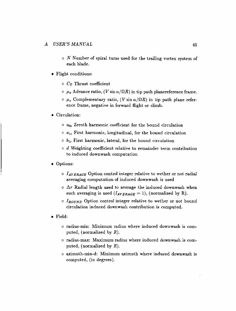
0 CR Vortex core radius, normalized by R

0 N Number of spiral turns used for the trailing vortex system of each blade.

8 COMPUTATIONS 29

0 aoc Zeroth harmonic coefficient for the bound circulation

0 al, First harmonic, longitudinal, for the bound circulation

0 bl , First harmonic, lateral, for the bound circulation

0 d Weighting coefficient relative to remainder term contribution to induced downwash computation

0 I A v E R A G E Option control integer relative to wether or not radial av- eraging computation of induced downwash is used

0 N M E ~ N Number of divisions of one sector used to average the in- duced downwash over azimuth. (One sector is the angle between two successive blades, i.e. (27r /b)

0 AT Radial length used to average the induced downwash when such averaging is used

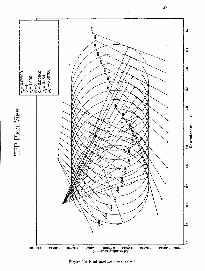
8.2 First module visualization Figure 10 shows the critical locations in the trailing vortex system as seen in projection in the tip path plane for a given point P at $p = 110 de- grees, TP = 1.3 and zp = 0.077 and for a given rotor position $? = 200 degrees. Each segment is indexed by &,de, i~ and another index j = 1,2, respectively. There are two segments ( j = 1,2) per spiral turn.

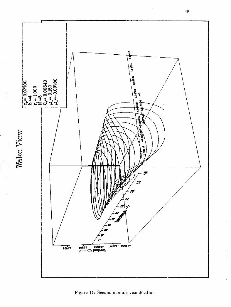
8.3 Second module visualization Figure 11 shows the geometry of the distorted trailing vortex system as seen in perspective from downstream.

8.4 Induced downwash computations Induced velocities itre given in terms of At, reduced induced inflow ratio,

8 COMPUTATIONS 30

where A; is the induced inflow ratio:

and AiOR is the momentum value of induced inflow ratio at hover:

Thus, a positive value corresponds to an induced downwash and a value of 1 corresponds to A; = ~ ; o r r = - JG = -0.056

8.4.1 Three dimensional plots

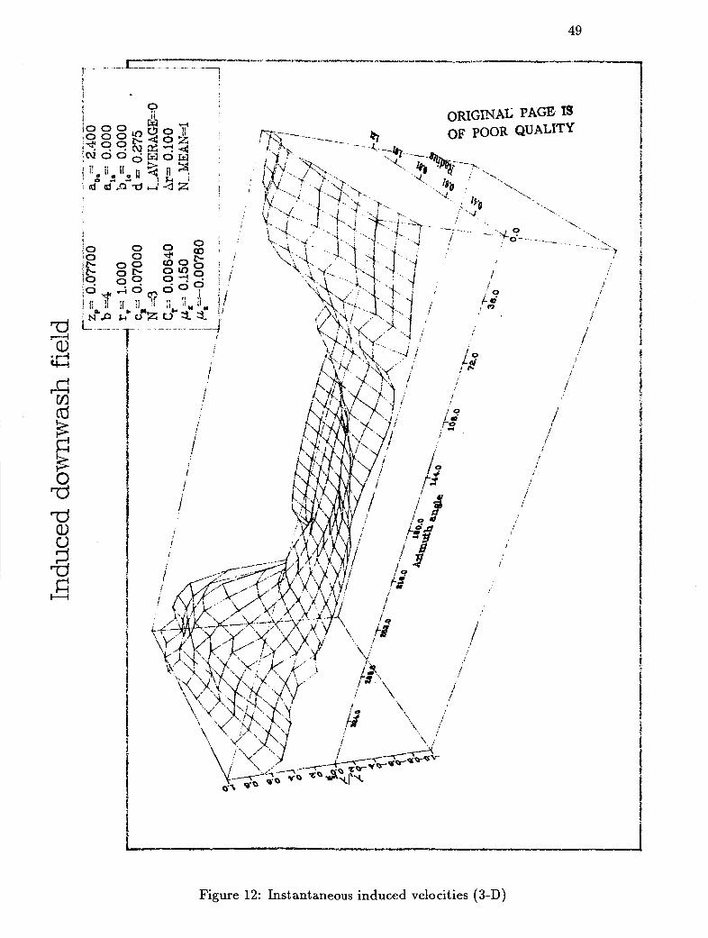
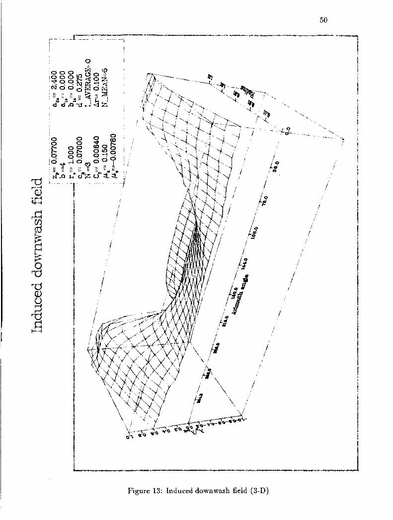
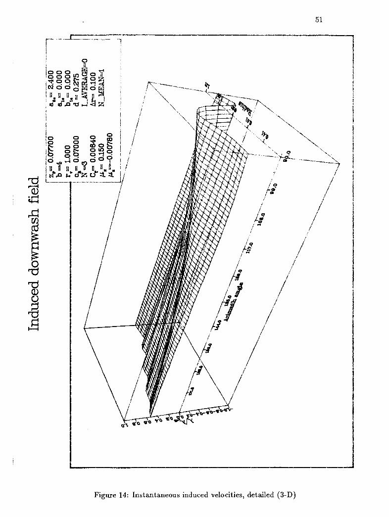
Plots 12, 13 and 14 are three dimensional plots where positive values at a surface point mean a downwash. The parameters used are the baseline values and they are modified in the subsequent plots. These parameters appear on the right-hand corner of each plot.

0 Figure 12 shows the plot of the induced downwash seen by a rotating blade from azimuth $r of 0 to 360 degrees along the span from .2 to 1.2 radial position (non dimensionalized by R). The blade is seen to encounter regions of downwash everywhere except at the leading edge of the rotor disc in addition to ridges encountered frontally.

0 Figure 13 shows a plot of the induced downwash field on the region of azimuth 0 to 360 degrees along a radial position from .2 to 1.2 (non dimensionalized by R). Five averaging divisions of a rotor sector ( N M E A N ) have been used. It can be seen that this plot is very similar to the preceding plot but it is smoother. Thus, the instantaneous induced downwash seen by a rotating blade and induced downwash field are very similar. This property is used in the subsequent compu- tations to evaluate the effect of the various parameters without going through the averaging process.

0 Figure 14 shows a plot of the induced downwash seen by a rotating blade from azimuth $r of 90 to 180 degrees along the span from .2R to 1.2R. This more detailed grid shows ridges encountered by the blade in a perpendicular fashion.

8 COMPUTATIONS 31

8.4.2

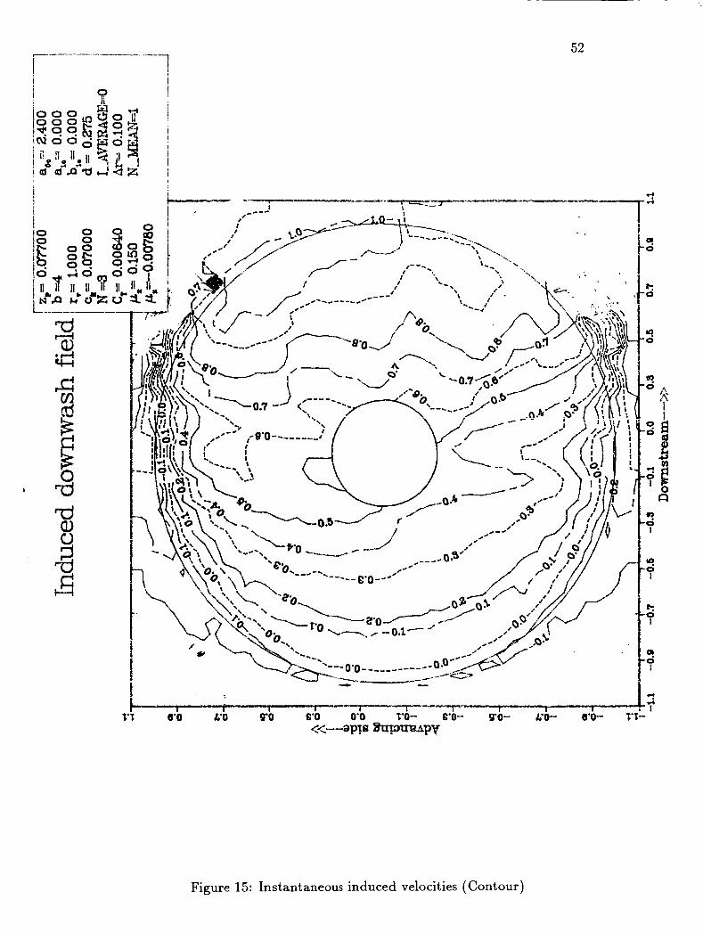
The following plots are contour plots where positive values at a point on the rotor disc mean a downwash. Most computation meshes extend from .2R to 1.2R and the plots are truncated at 1.1R. The lower and higher bounds of the radial positions of computed points can be changed at will, as can the truncation radial position for plotting.

Contour plots, influence of input parameters

0 Figure 15 shows the contour plot of the induced downwash seen by a rotating blade from azimuth ?+hr of 0 to 360 degrees along the span from .2R to 1.1R. This plot contains the same information as Figure 12. No radial averaging is used, no bound circulation contribution is present and the first harmonic coefficients of the circulation are set to zero.

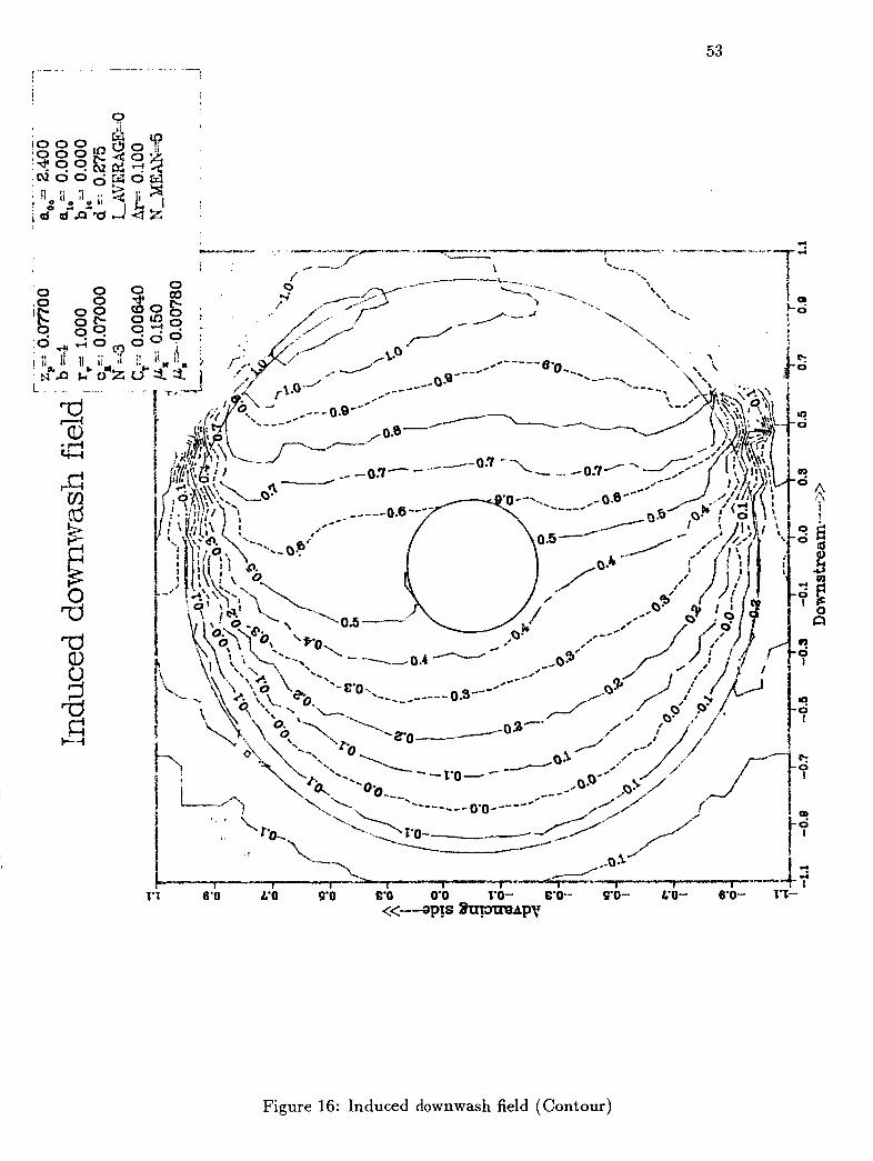
0 Figure 16 shows the contour plot of the induced downwash field on the region or' azimuth 0 to 360 degrees from 211 to i . lR. This piot contains the same information as Figure 13 and has the same param- eter settings as in the preceding plot except for N M E A N which is set equal to 5, to average the velocities seen around the rotor as the rotor rotates by one sector in 5 increments. It is apparent that a region of upflow appears at the leading edge of the rotor disc. Compared with the experimental results obtained in reference [5] illustrated in Figure 34, there is a good agreement in the trends from fore to aft of the rotor disc. Also, an upflow on each side of the disc, downstream of 90 degrees and 270 degrees is obtained. The magnitudes of the downflow on the aft portion of the rotor are the same, providing an B priori confirmation for the values of aoe and d as valid.

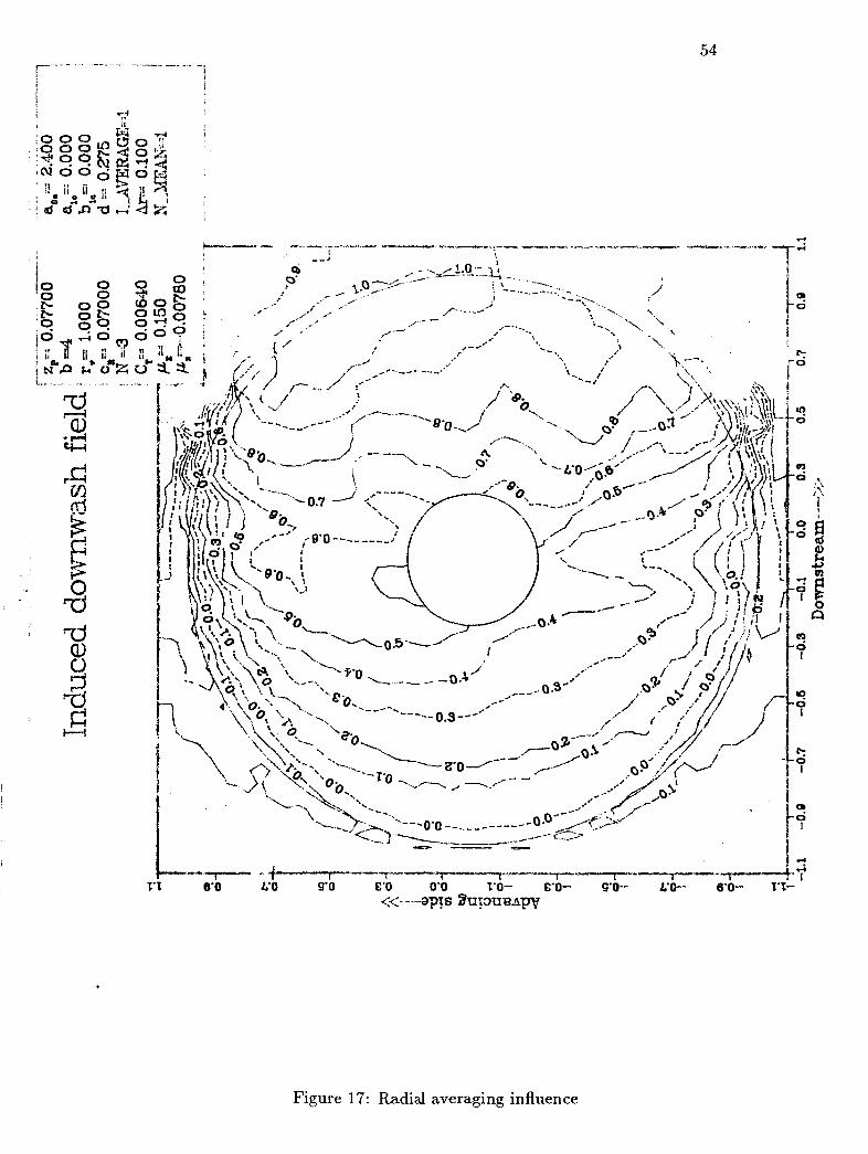
0 Figure 17 shows that the application of the option of radially averaged induced velocity gives similar results than when not used (comparison with Figure 15).

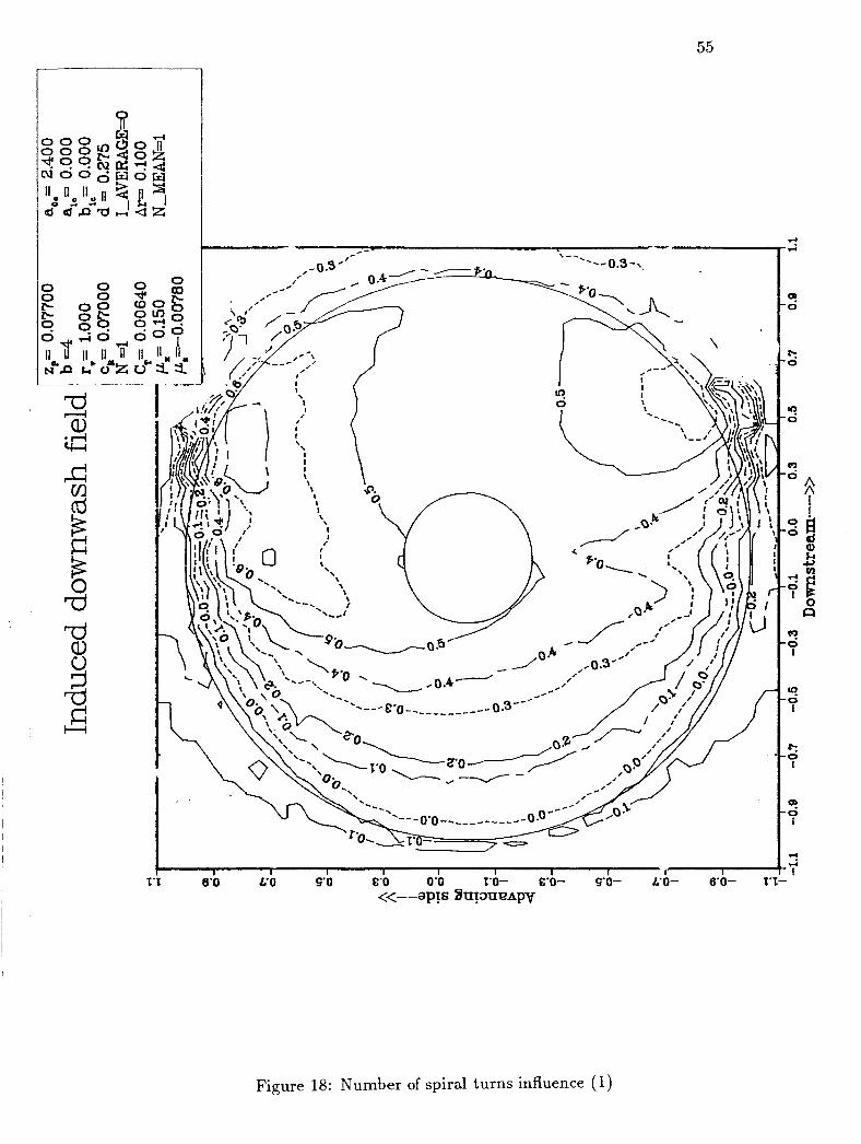
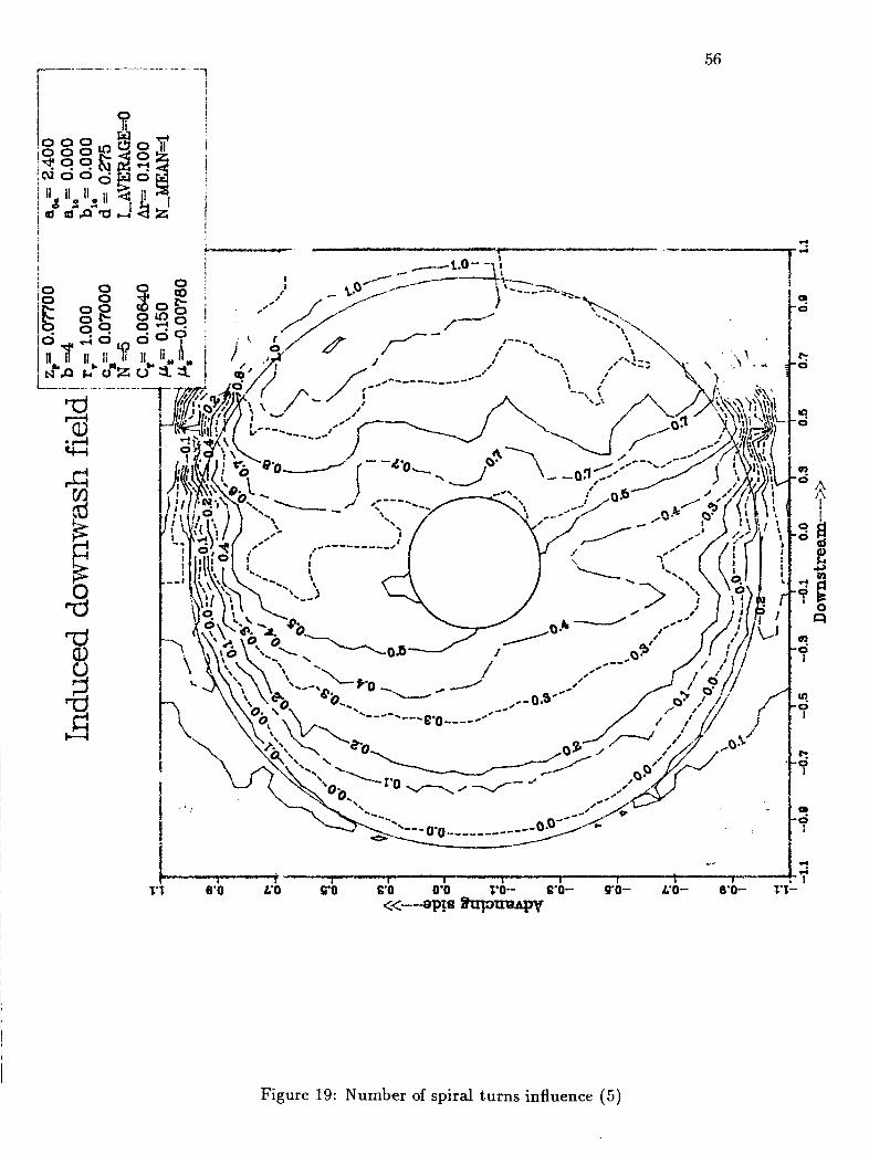
0 Figure 18 and 19 show the influence of the number of spiral turns taken into account for the trailing vortex system. N = 1 in Figure 18 is too low. Neither trends nor magnitudes are approximating exper- imental results of Figure 34. However, it is seen that N = 5 gives almost the same results as N = 3 (Figure 15). It is safe as a conse-

8 COMPUTATIONS 32

quence to retain three turns trailed by each blade for the subsequent computations.

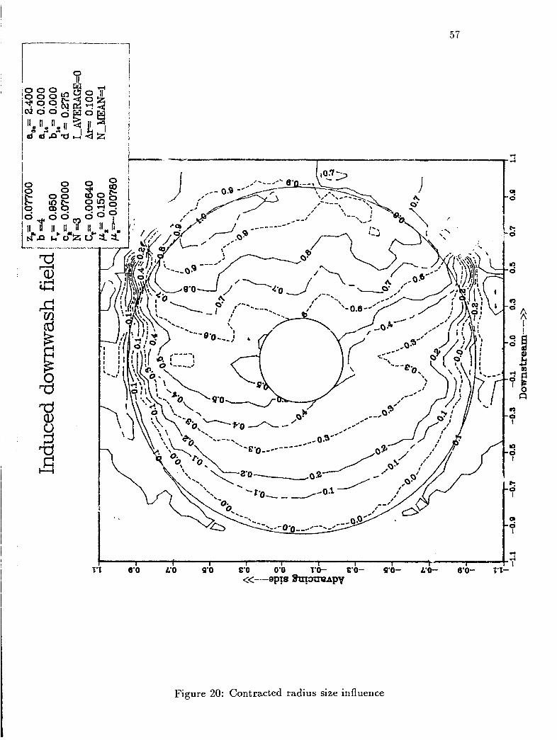
0 Figure 20 shows that the contracted radius r , is not a sensitive value for the induced velocity in the rotor disc by comparison with Fig- ure 15.

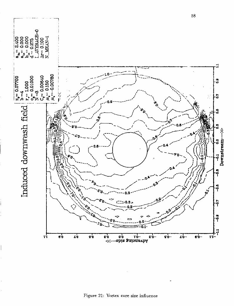
0 Figure 21 shows slightly more definition of the induced downwash seen by a rotating blade for a smaller vortex core radius CR although the sensitivity is not very high (comparison with Figure 15). It is, however the only parameter of the present model through which the aspect ratio effects of the rotor blades can be represented since the vortex core radius certainly bears some relationship to the relative size of the chord c and the blade radius R.

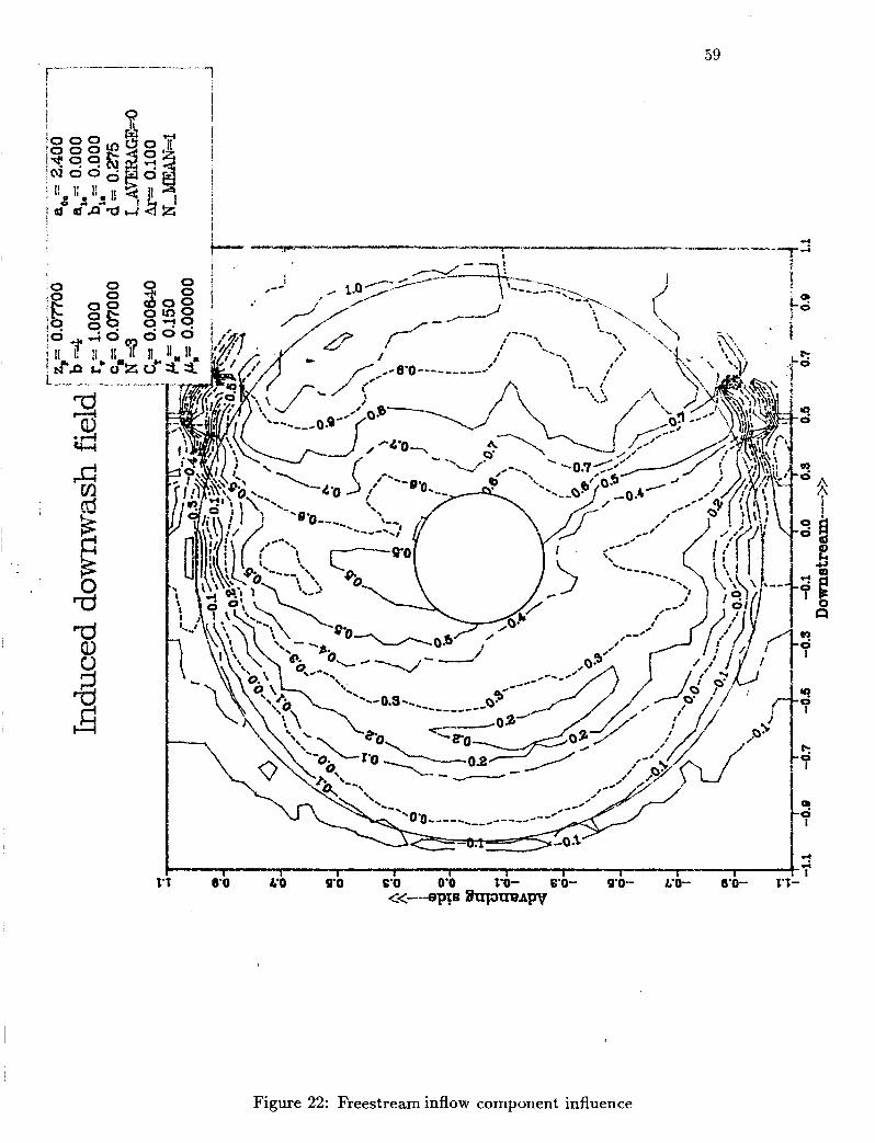
0 Figure 22 shows the influence of the flight condition variable pz on the induced downwash seen by a rotating blade by comparison with the baseline case Figure 15. Zero freestream inflow component (pz = 0. i.e a = 0) seems, as expected, to bring more irregularities in the induced downwash contour patterns, since the trailing vortex system stays in the tip path plane longer than for a negative value of pz.

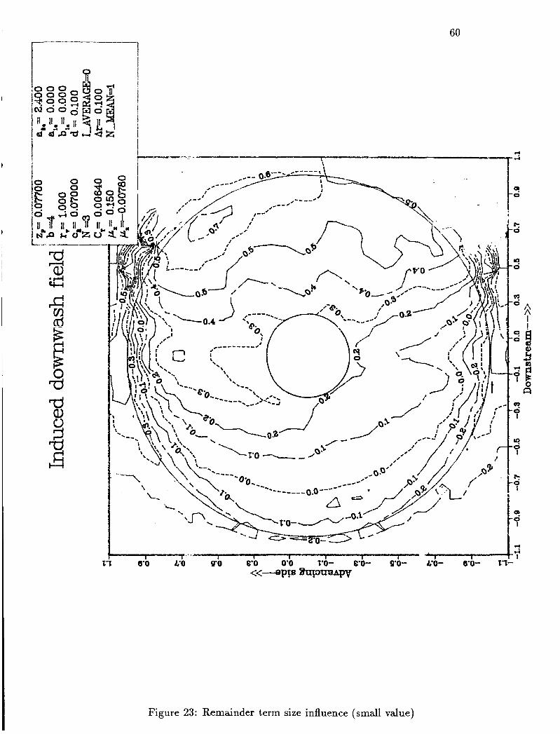
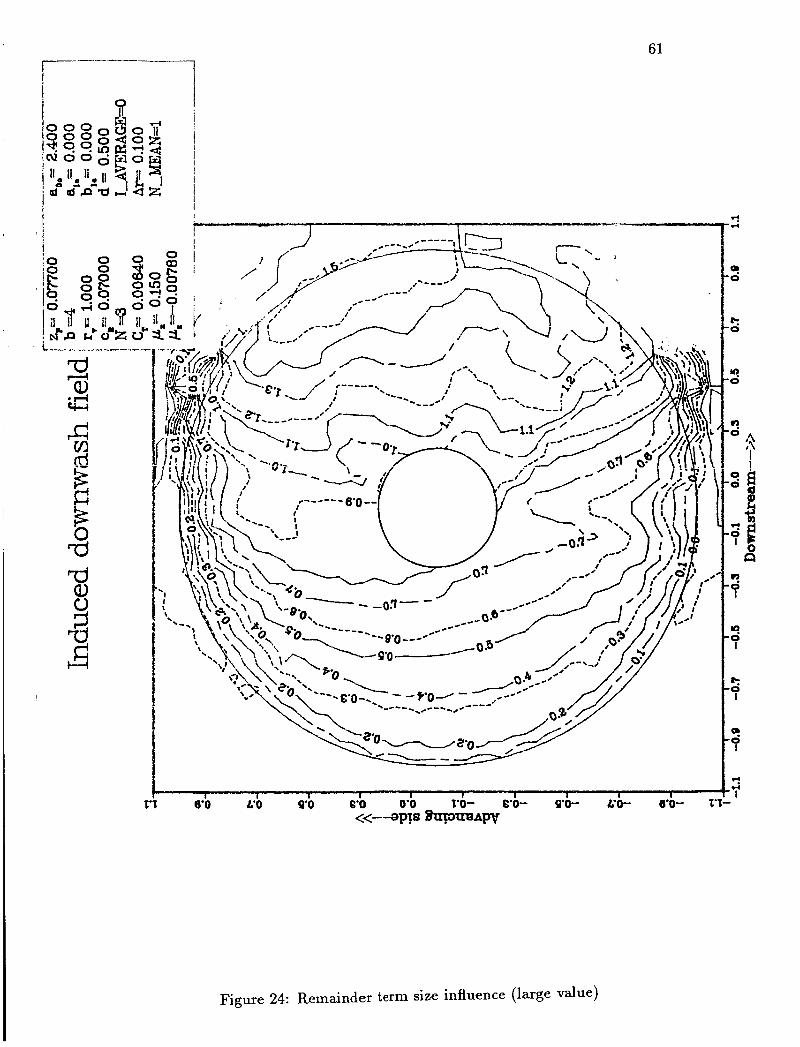
0 Figure 23 and 24 show the influence of the remainder part of the spiral turns contributions through the parameter d. It is seen to affect in a uniform way the whole rotor disc and the magnitude of .275 is confirmed as adequate.

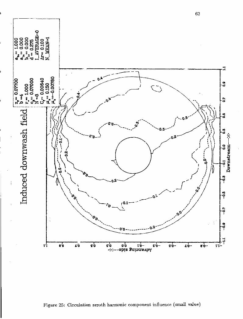
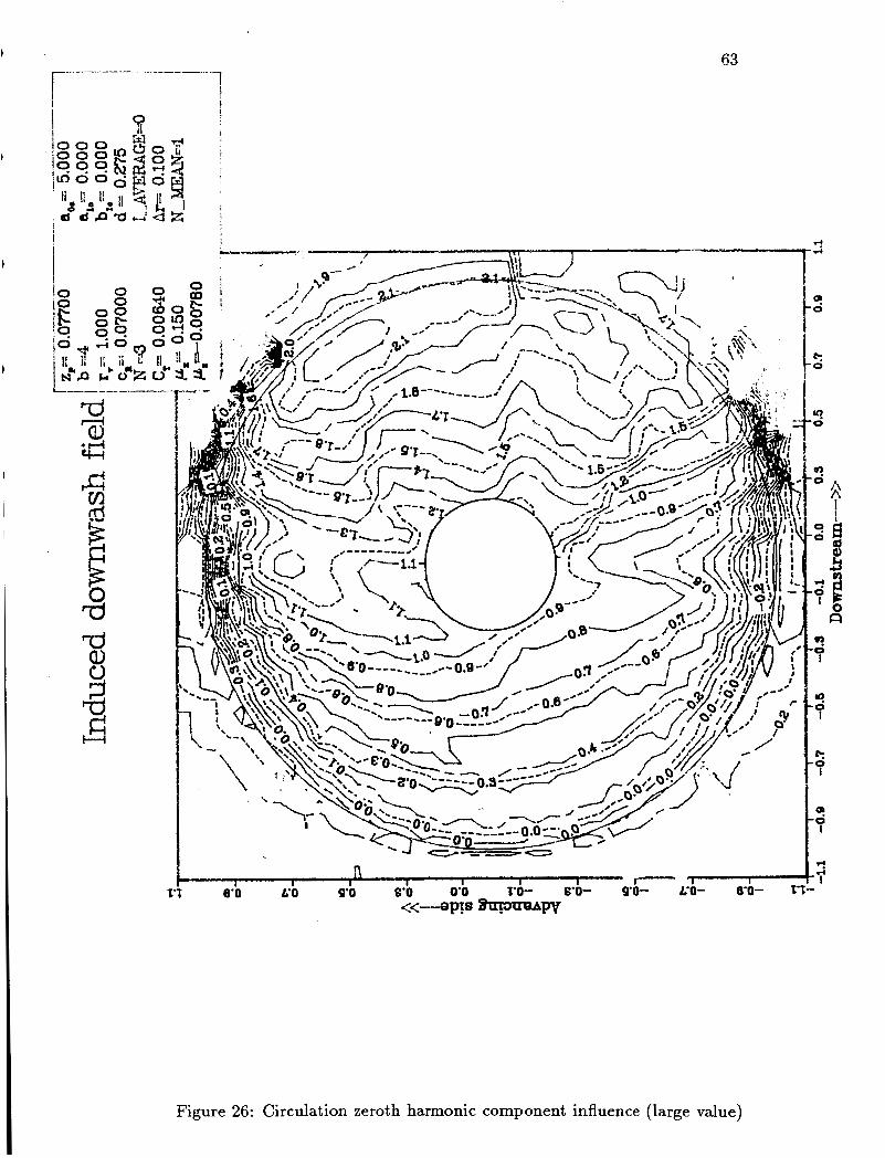
0 Figure 25 and 26 show the influence of the zeroth harmonic compo- nent of the circulation through the parameter aoc. Here, it is seen that it influences the steepness of the fore to aft slope of induced downwash. The maximum downwash magnitude can thus be taken to size this parameter and the value of 2.4 is adequate.

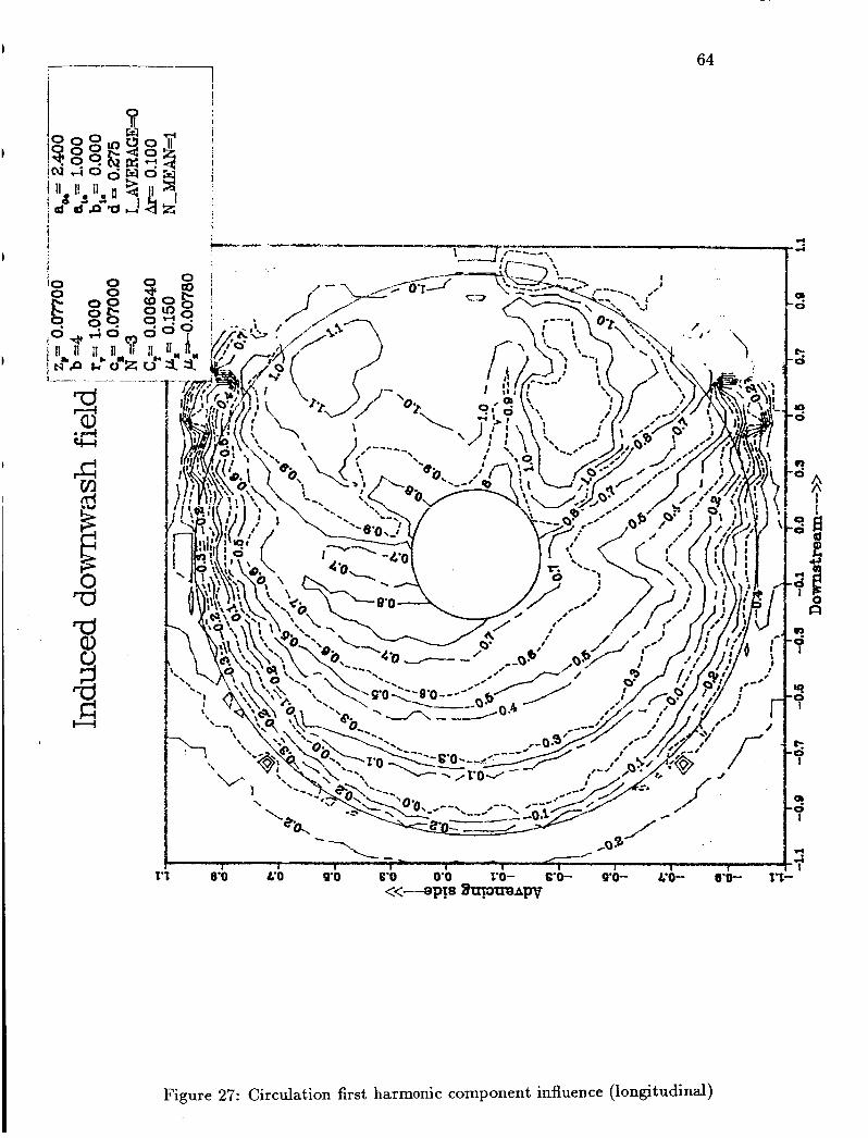
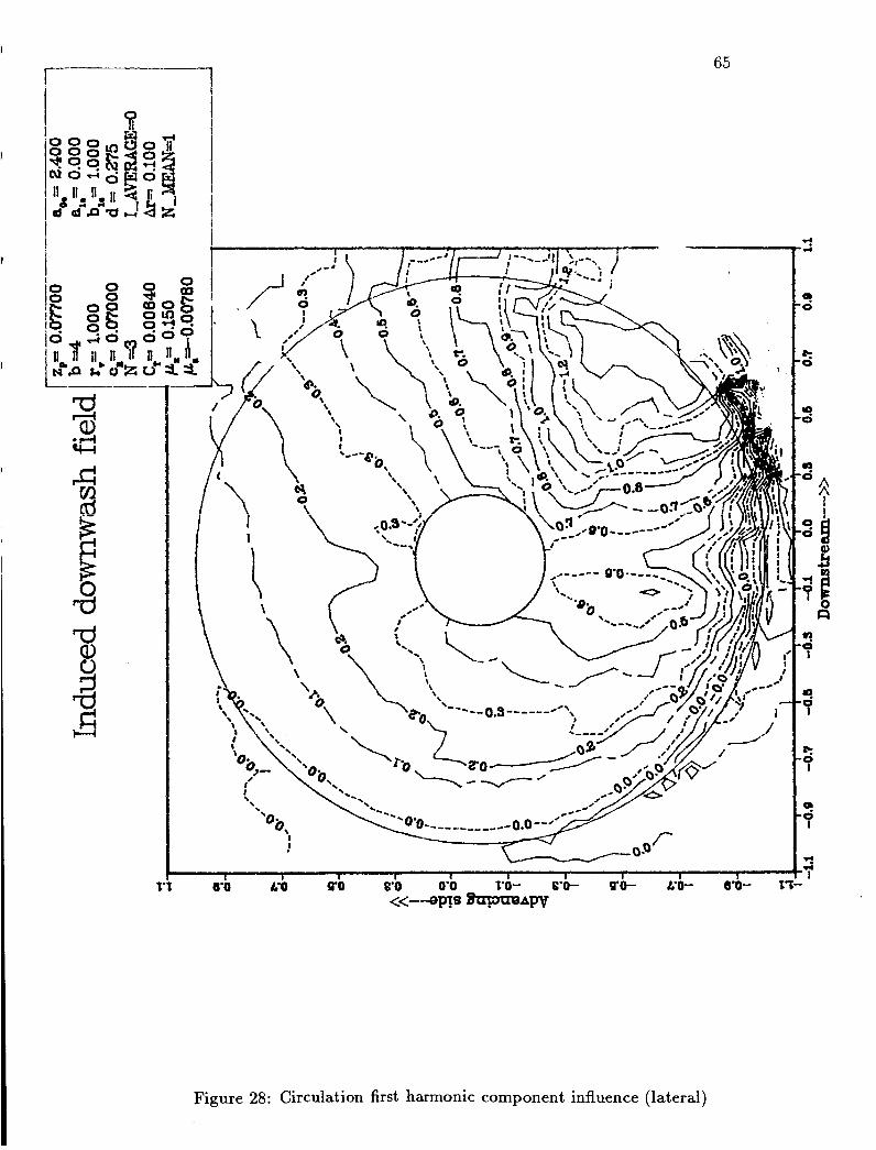
0 Figure 27 and 28 show the influence of the first harmonic components of the circulation through the parameters alc and blc . The asymmetry of the induced downwash pattern is clearly apparent here.

8 COMPUTATIONS 33

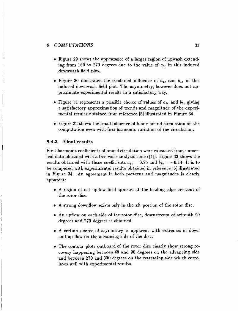
0 Figure 29 shows the appearance of a larger region of upwash extend- ing from 160 to 270 degrees due to the value of alc in this induced downwash field plot.

0 Figure 30 illustrates the combined influence of al, and blc in this induced downwash field plot. The asymmetry, however does not ap- proximate experimental results in a satisfactory way.

0 Figure 31 represents a possible choice of values of al, and blc giving a satisfactory approximation of trends and magnitude of the experi- mental results obtained from reference [5] illustrated in Figure 34.

0 Figure 32 shows the small influence of blade bound circulation on the computation even with first harmonic variation of the circulation.

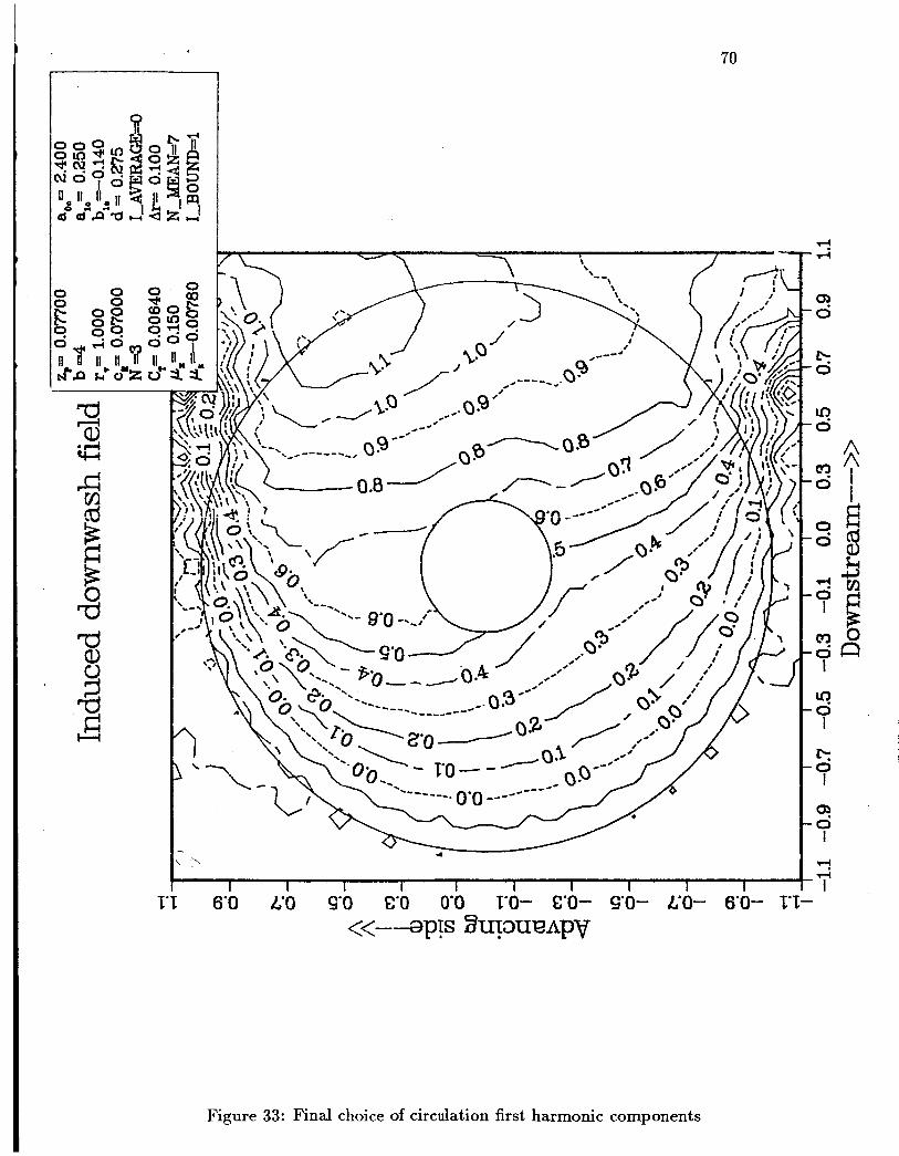
8.4.3 Final results

First harmonic coefficients of bound circulation were extracted from numer- ical data obtained with a free wake analysis code ([4]). Figure 33 shows the results obtained with those coefficients alc = 0.25 and bl, = -0.14. It is to be compared with experimental results obtained in reference [5] illustrated in Figure 34. An agreement in both patterns and magnitudes is clearly apparent:

0 A region of net upflow field appears at the leading edge crescent of the rotor disc.

0 A strong downflow exists only in the aft portion of the rotor disc.

0 An upflow on each side of the rotor disc, downstream of azimuth 90 degrees and 270 degrees is obtained.

0 A certain degree of asymmetry is apparent with extremes in down and up flow on the advancing side of the disc.

0 The contour plots outboard of the rotor disc clearly show strong re- covery happening between 60 and 90 degrees on the advancing side and between 270 and 300 degrees on the retreating side which corre- lates well with experimental results.

8 COI1IP UTATIOhTS 34

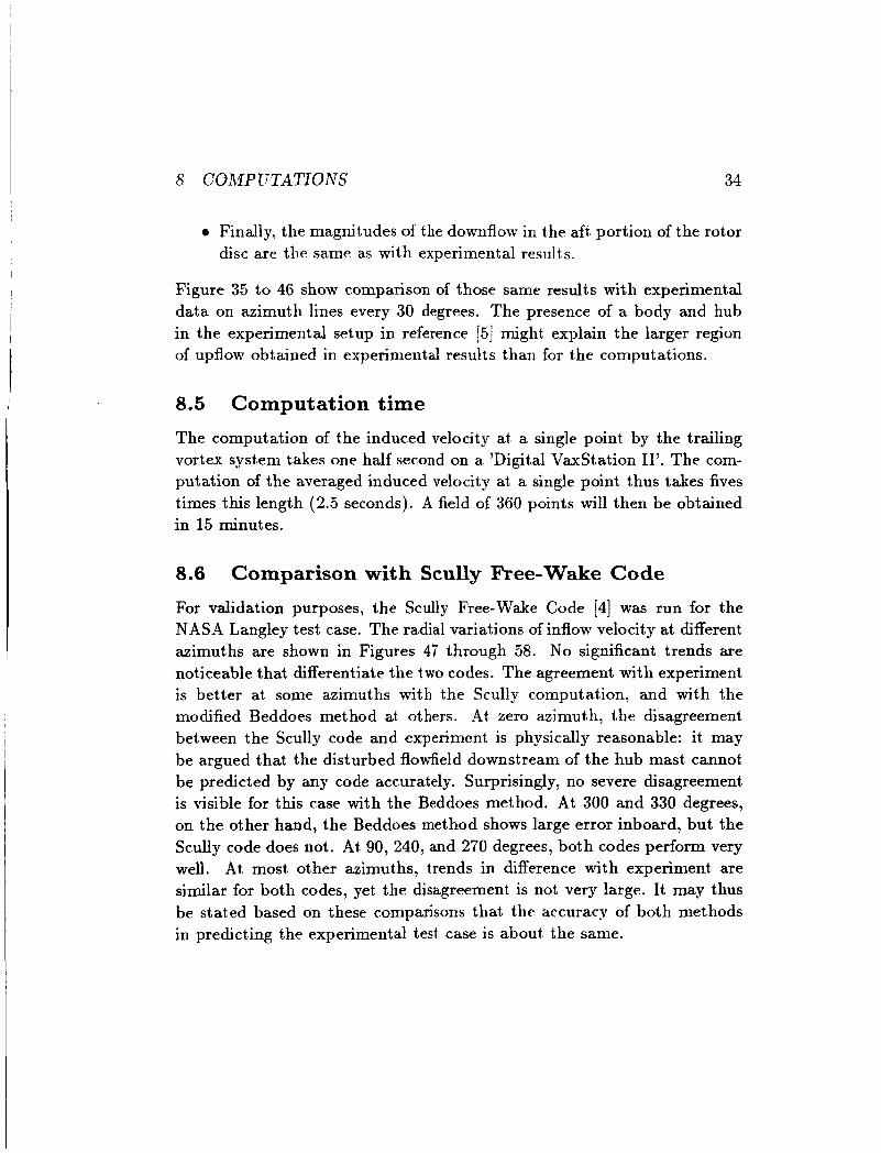
0 Finally, the magnitudes of the downflow in the aft, portion of the rotor disc are the same as with experimental results.

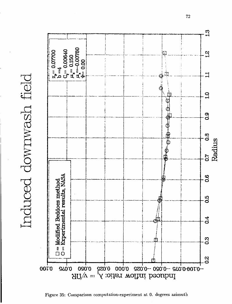
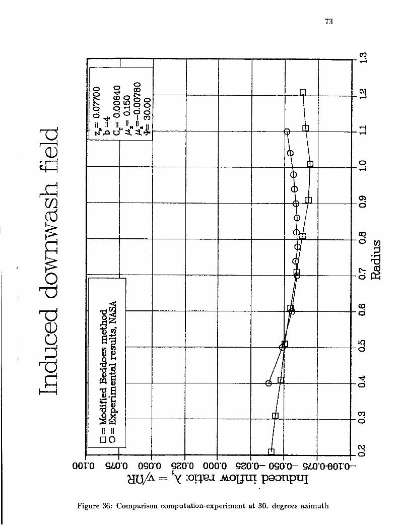
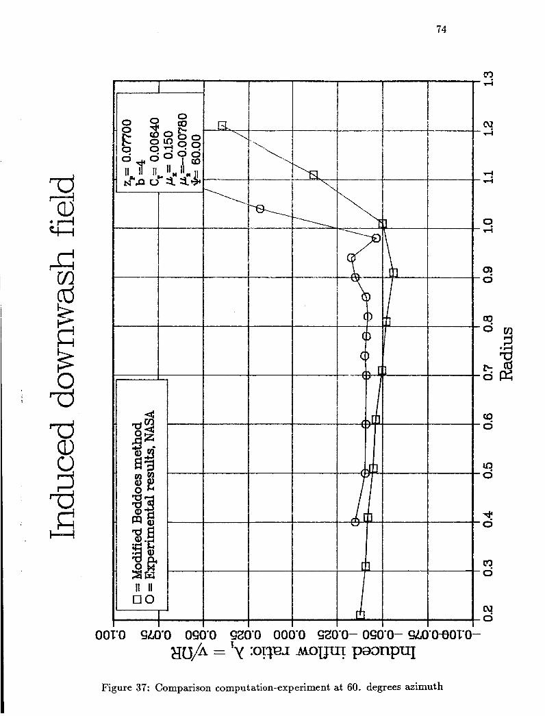
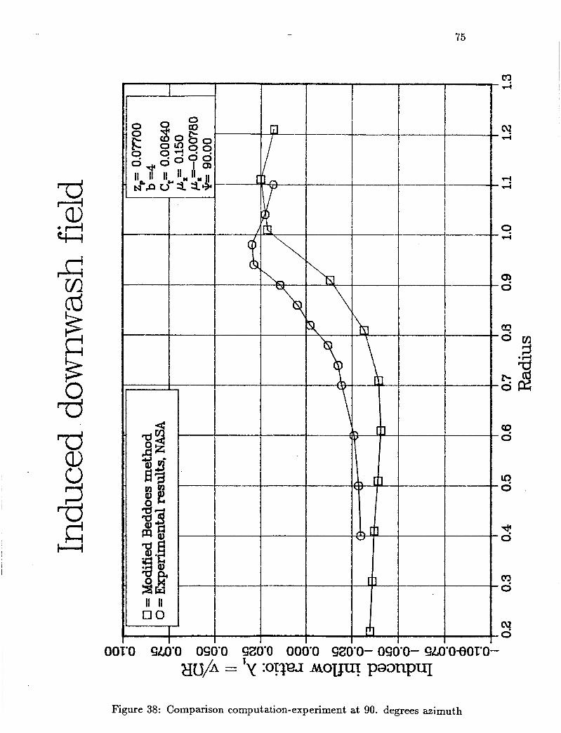
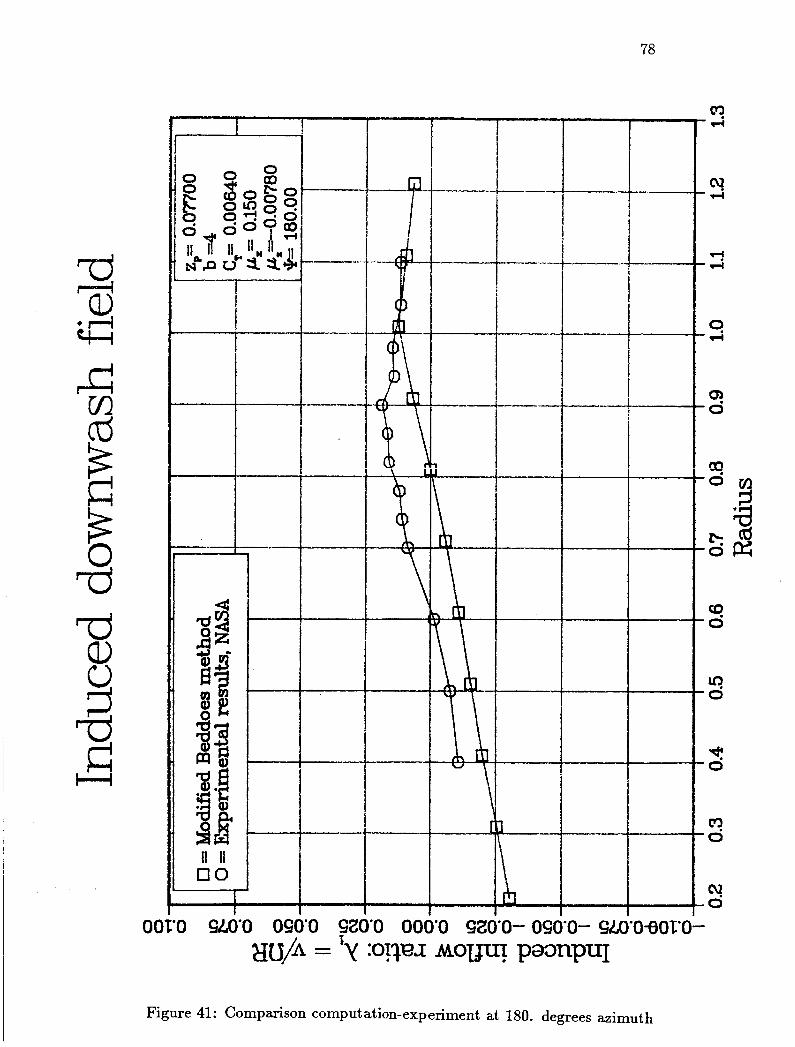
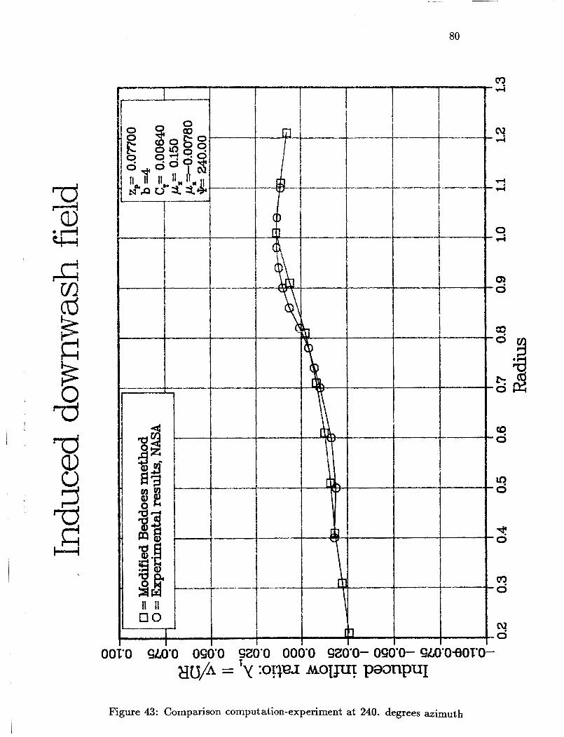
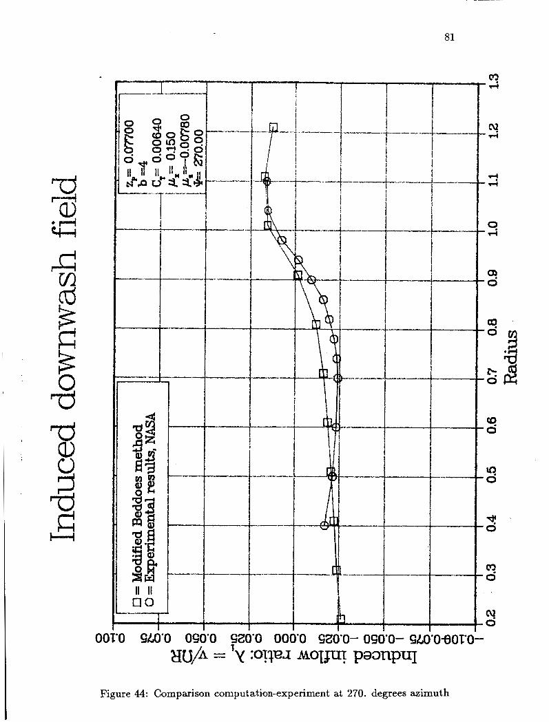
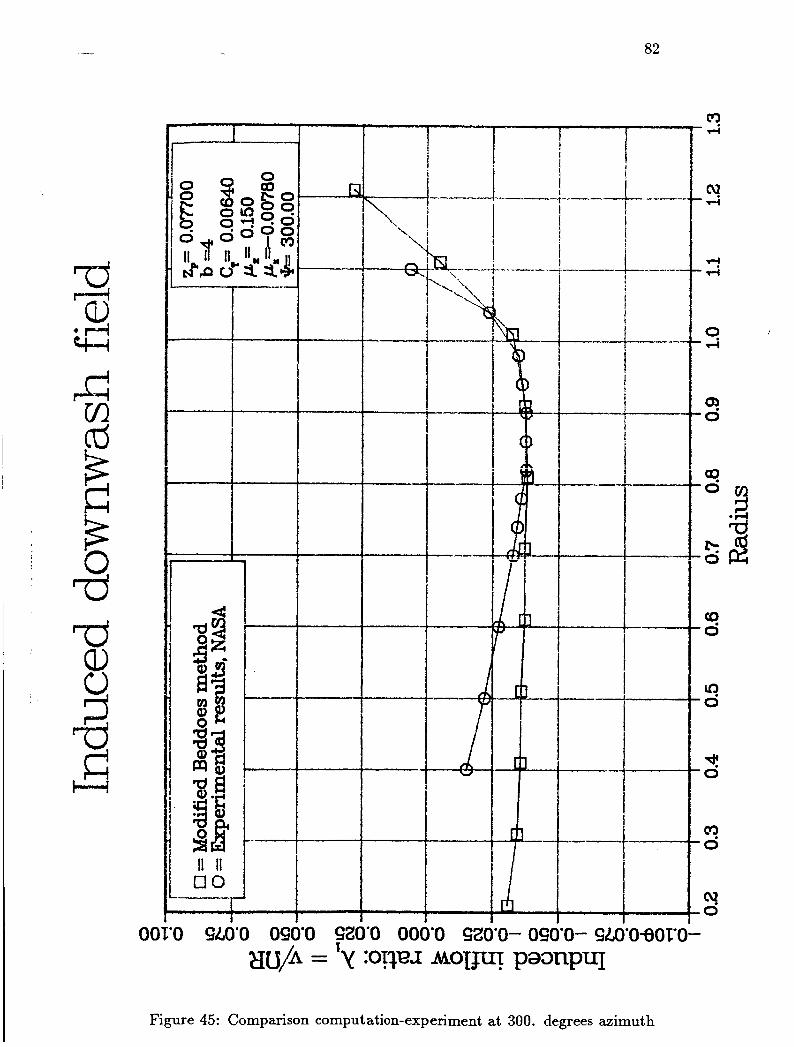
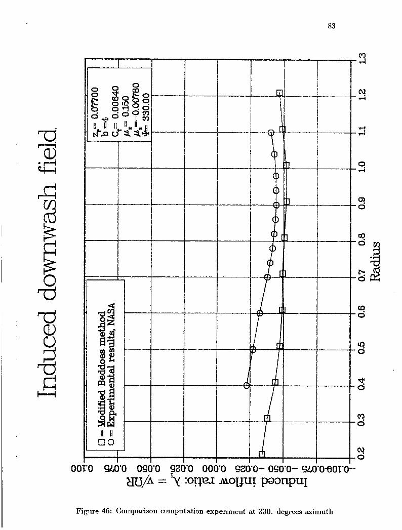
Figure 35 to 46 show comparison of those same results with experimental data on azimuth lines every 30 degrees. The presence of a body and hub in the experimental setup in reference [5] might, explain the larger region of upflow obtained in experimental results than for the computations.

8.5 Computation time

The computation of the induced velocity at. a single point. by the trailing vortex syst.eni takes one half second on a 'Digital VaxStation II'. The com- putation of the averaged induced velocity at a single point thus takes fives times this length (2.5 seconds). A field of 360 points will then be obtained in 15 minutes.

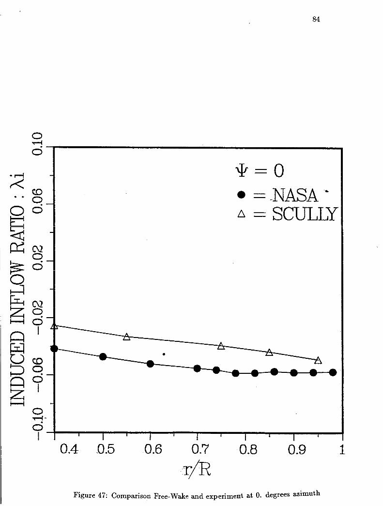
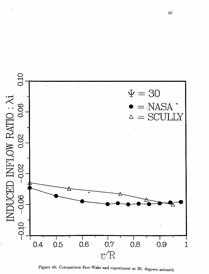
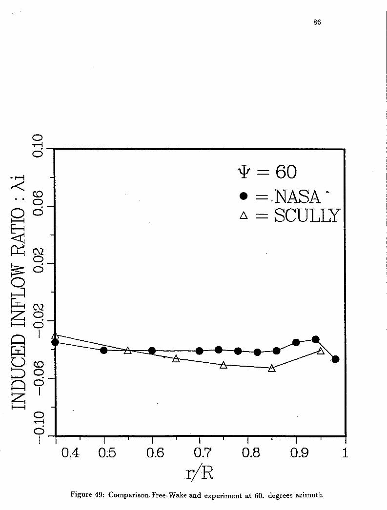
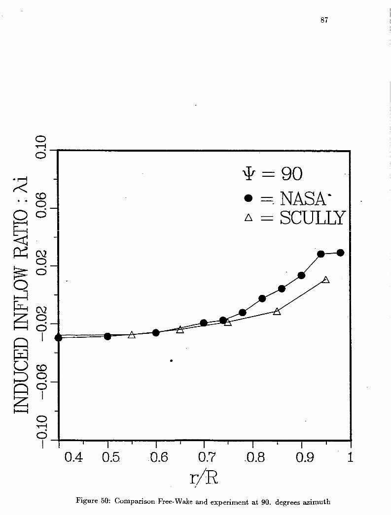
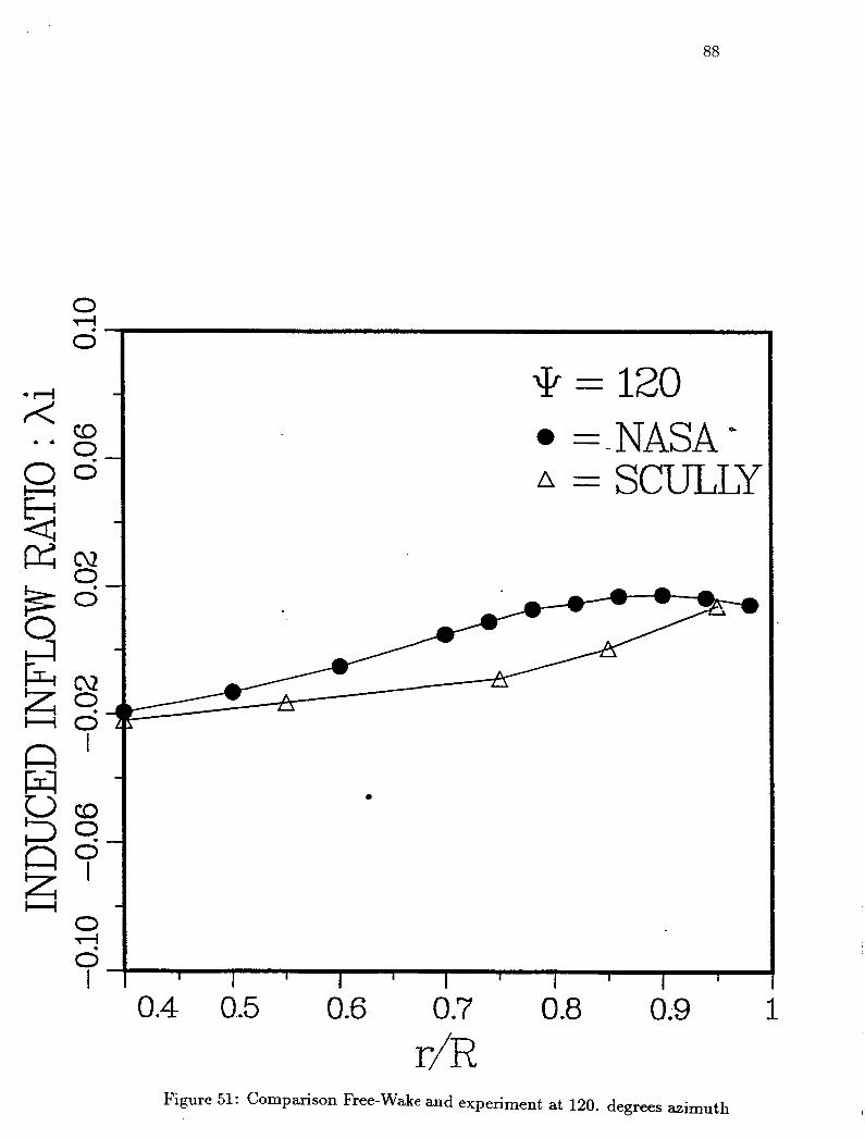
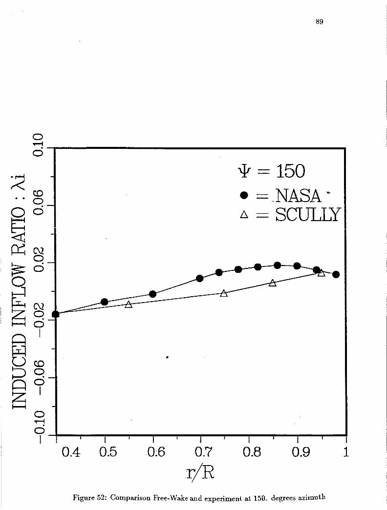
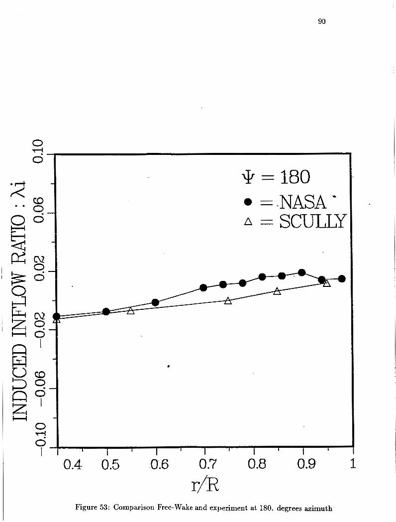
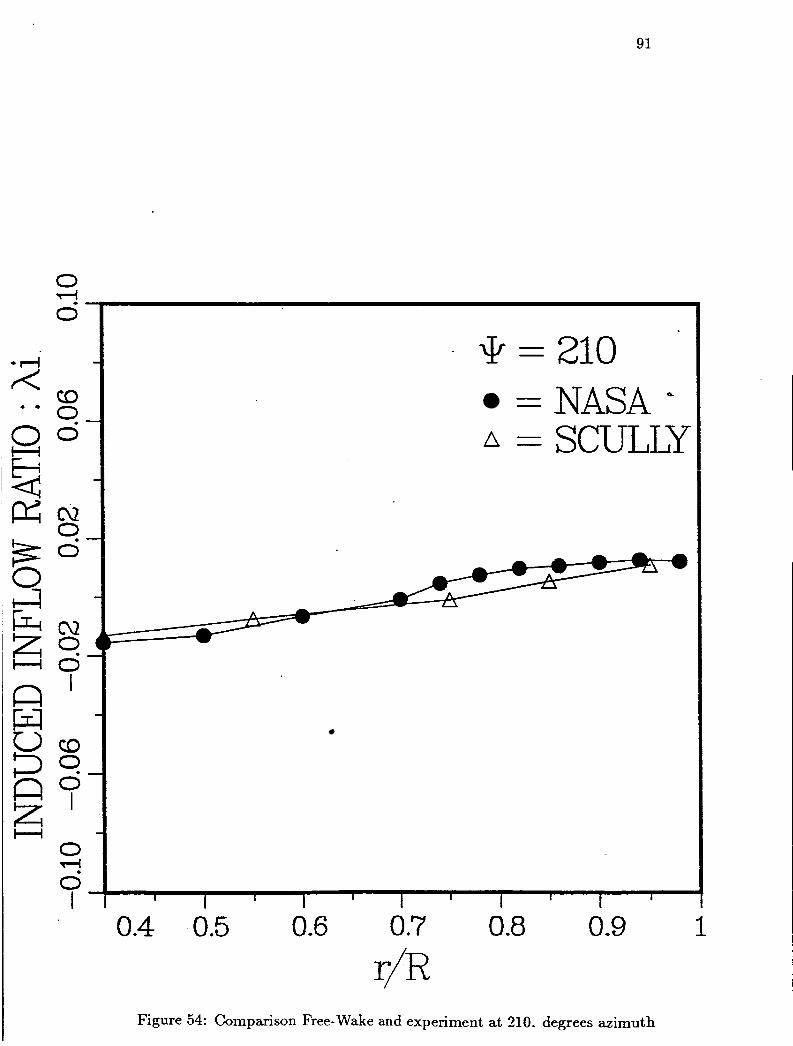
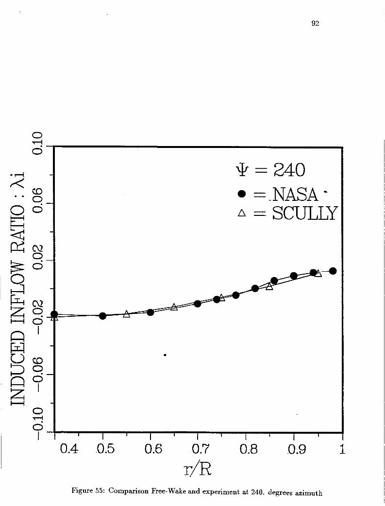
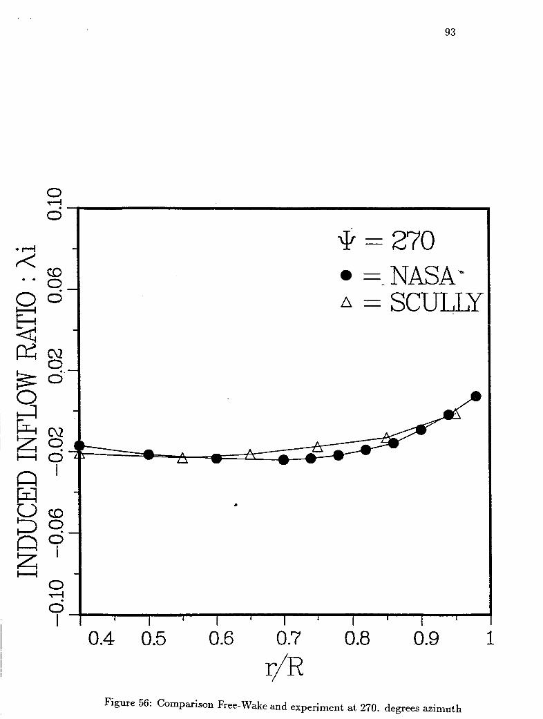
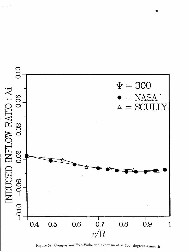
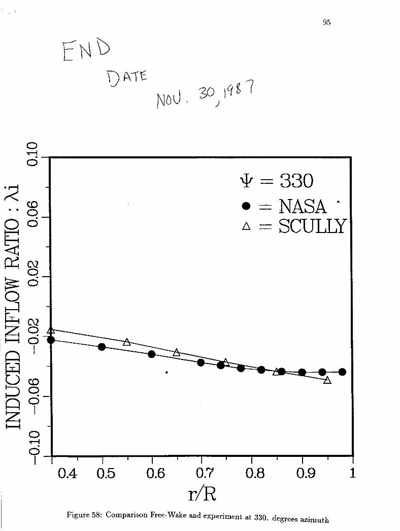
8.6 Comparison with Scully Free-Wake Code For validation purposes, the Scully Free-Wake Code [4] was run for the NASA Langley test. case. The radial variations of inflow velocity at different azimuths are shown in Figures 47 through 58. No significant trends are noticeable that differentiate the two codes. The agreement with experiment is better at some azimuths with the Scully computation, and with the modified Beddoes method at others. At zero azimuth, the disagreement between the Scully code and experiment is physically reasonable: it may be argued that the disturbed flowfield downstream of the hub mast cannot be predicted by any code accurately. Surprisingly, no severe disagreement is visible for this case with the Beddoes method. At 300 and 330 degrees, on the other hand, the Beddoes method shows large error inboard, but the Scully code does not. At 90, 240, and 270 degrees, both codes perform very well. At most other azimuths, trends in difference with experiment are similar for both codes, yet the disagreement is not very large. It may thus be stated based on these comparisons that the accuracy of both methods in predicting the experimental test case is about the same.

9

35

Capabilities of the code

9.1 Capabilities The test case computed with the present scheme (Figure 33) shows good agreement with experimental results obtained in reference [5] for a short computation time. Interesting results can otherwise be observed as to the similarity of instantaneous induced downwash seen by a rotating blade and induced downwash field plots. Different options and parameter values can also be used to study their influence on the results obtained and assess their sensitivity for a given rotor and flight conditions:

0 Utilization of radial averaging and the variation of the averaging in- terval used.

0 Variation of vortex core radius CR

0 Introduction of first harmonic variation of circulation strength over the trailing vortex system and on the blade bound vorticity.

0 Variation of the contracted radius T,

0 Variation of the number of trailing vortex system turns taken into consideration

0 Variation of the number of increments over which the induced down- wash is averaged over azimuth (A reasonable number is 7) .

Factors to be considered in judging the completeness of the model are the presence of a shed vortex system, close blade vortex interaction, lifting surface effects, inboard trailing wake system and presence of a body and hub as is the case for the experimental case in reference [5]. This last point might explain the larger region of upflow obtained in experimental results than for this model.

9.2 Potential for growth

The model implemented in this report is a simple wake model representing the trailing vortex system in an original way. Adding a shed vortex system,

9 CAPABILITIES OF THE CODE 36

an inboard trailing wake system, close blade vortex interaction and lifting surface effects, may not be consistent with the simplicity and peculiarity of the trailing vortex system model. The code might see its computation time increase to a level comparable to that of free wake codes and other much more refined wake models without having solid analytical consistency. On the other hand, adding those features might provide some insight on their relative importance in a wake model.

9.3 Adaptability to interaction problems The wake model discussed in this report has its most fundamental charac- teristic in the geometry of its prescribed trailing vortex system. Each spiral trailing from the rotor has a projection in the tip path plane in the form of a regular cycloidal curve. This allows it to have the property of having only two tangents per turn which are perpendicuiar to the line joining iiie point of tangency to a given point where the induced velocity is computed. This property is fundamental to the present model consisting in computing the induced velocity by two staight vortex segments and a remainder term. It is also fundamental to the algorithm that searches for critical locations of those straight vortex segments. The interaction problem, consisting in distorting the shape of the trailing vortex system would result immediately in the loss of the geometrical property and render impossible the implemen- tation of both the model and its algorithm. Thus, this model appears to be unattractive for extension to problems involving complex vortex distortion effects.

10 Conclusions

The test case computed with the present scheme (Figure 33) shows good agreement with experimental results obtained in reference [5] for a short computation time. The capabilities of the model include the study of cer- tain parameter influences on the results obtained and an assessment. of their sensitivity for a given rotor and flight. conditions. The model is by no means a complete wake model and it is possible to refine it and add some feat,ures like a shed vortex system, an inboard trailing wake system. close blade vortex interaction and lifting surface effects. Due to its peculiarity, the present model is not suitable to be evolved into a part of an interaction problem wake model. This model makes it possible to obtain a description of a rotor’s induced downwash field with very small computer resources, both in memory and time, in a workstation-type of environment. The per- formance of the model has been compared to that of the Scully Free-Wake code in predicting the extensive inflow velocity data base recently acquired at NASA Langley for a four-bladed rotor. The accuracy of the model is seen to be quite similar to that of the Scully code, and trends are also similar. Yet the present model can be run on a workstation in interactive mode, whereas the Scully code requires a larger mainframe computer where it has to be run as a batch job for economic reasons. In conclusion, the model is an efficient and flexible tool for the preliminary evaluation of the induced velocity field of a rotor.

11 Acknowledgements The authors gratefully acknowledge the assistance provided by Mr. John Berry of the U.S. Army Aerostructures Directorate, NASA Langley Re- search Center in providing them with the Inflow data base, and in several valuable discussions. They are also grateful to Mr. Dmitri Mavris, who pro- vided them with the comparisons obtained between the Scully Free-Wake Code and the NASA results.

38

References

[l] Beddoes T.S., Westland Helicopters Ltd. A wake model for high reso- lution airloads.

[2] Egolf T.A., Landgrebe A.J. Generalized wake geometry for a helicopter rotor in forward flight and effect of wake deformation on airloads. A.H.S. Annual Forum 1984.

[3] Heyson H.H., Katzoff S. Induced velocities near a lifting rotor with nonuniform disk loading. NACA Report 1319,1956.

[4] Scully M.P. Computation of helicopter rotor wake geometry and its influence on rotor harmonic airloads. ASRL TR178-1, 1975.

r c i 11'1 D-,,,,. u c ; l l y J.D., E ~ a d D.R., Ee!!!ztt J.W., Althoff S.L: Helicopter ro- tor induced velocities theory and experiment. Rotorcraft Aerodynam- ics Office. Aerostructures Directorate, USAARTA-AVSCOM, Langley Research Center, Hampton, Virginia. Presented at the AHS Special- ists' Meeting on Aerodynamics and Aeroacoustics, Arlington, Texas, February 25-27, 1987.

[6] ISSCO Disspla Manual.

39

A User’s Manual

A.l Introduction Three modules perform the computations. They are independent from the pre and post processing. The first module is Location and finds the critical locations in the tip path plane of the trailing vortex system. The second module is Wake and comprises the subroutine computing the momentum values of induced downwash as well as the vertical distorted geometry of the trailing vortex system. The third module is Velocity and computes the induced velocity at a given point. Each of the modules can be used through a pre and post processor:

0 Location is used by Test-Location

0 Wake is used by Test-Wake

0 Velocity is used by Test-Velocity

Each module is thus testable independantly if the tests are effected in the order going from module 1 to module 3. Indeed, the second module calls the first module; the third module calls the second module which then calls the first module. A front-end program, Frontal is used to produce 3-D plots and contour plots of induced velocitycomputed by Velocity. All three test programs and Frontal use the same input file called Input.

A.2 First module The first module Location finds the critical locations in the trailing vortex system for a given point P and for a given rotor position &. Test-Location shows these locations in the trailing vortex system as seen in projection in the tip path plane (Figure 10). Each segment is indexed by &ade, i~ and another index j = 1,2, respectively. There are two segments ( j = 1,2) per spiral turn. The input data is the following and is input through the unique input file Input:

0 Screen:

A USER'S MANUAL 40

o I-PLOTTER: Indicator of plot routing (0 for screen, 1 for plot- ter).

0 Point position; the position of point P:

o ~ p : Radial coordinate of point P, normalized by R. o $p: Azimuth coordinate of point P in degrees.

o z p : z coordinate of point P, normalized by R.

0 Rotor position

o &: Azimuth angle of blade of reference, in degrees.

0 Rotor characteristics:

o L Niiiiibei d' b!iide~

o T , Contracted radius, normalized by R. The trailing vortex sys- tem is trailed from the T , radial locations.

o N Number of spiral turns used for the trailing vortex system of each blade.

0 Flight conditions:

o pz Advance ratio, (V sin a / R R ) in tip path planereference frame.

A.3 Second Module The second module Wake computes the momentum theory constants for the given flight conditions and the ordinates of the critical locations in the trailing vortex system. Test-Wake shows the geometry of the distorted trailing vortex system as seen in perspective from downstream (Figure 11). The input data is the following and is input through the unique input file Input:

0 Screen:

o I-PLOTTER: Indicator of plot routing (0 for screen, 1 for plot- ter).

A USER’S MANUAL

0 PLOTSD:

41

o PHI: Angle between a axis an^ vertical plane containing view point direction (degrees).

o THETA: Angle between horizontal plane and view point direc-

o RADIUS: distance of view point to the figure (the farther the view point, the most isometric perspective is obtained), (RA- DIUS=25 is standard)).

tion.

0 Rotor position

o &: Azimuth angle of blade of reference, in degrees.

0 Rotor characteristics:

o b Number of blades

o T , Contracted radius, normalized by R. The trailing vortex sys-

o N Number of spiral turns used for the trailing vortex system of

tem is trailed from the T , radial locations.

each blade.

0 Flight conditions:

o CT Thrust coefficient

o pz Advance ratio, ( V sina/RR) in tip path planereference frame.

o pz Complementary ratio, (V sin a/OR) in tip path plane refer- ence frame, negative in forward flight or climb.

A.4 Third Module The third module Velocity computes the induced velocity at a given point P by the trailing vortex system and optionally by the bound vortex system.

A USER’S MANUAL 42

A.4.1 Test-Velocity

Test-Velocity runs the module to be numerically tested with the debug- ger of the compiler. The computations are indeed traced out by extensive dumping throughout execution, of variable and parameter values. These values are then matched with hand calculations and correlation with geo- metrical insight available through the graphics generated by the first two modules. The results are given in term of At , reduced induced inflow ratio,

where A; is the induced inflow ratio:

and X i o a is the momentum value of induced inflow ratio at hover:

Thus, a positive value corresponds to an induced downwash and a value of 1 corresponds to A; = A i O H = -dm = -0.056 The input data is the following and is input through the unique input fde Input:

0 Point position; the position of point P:

o T P : Radial coordinate of point P, normalized by R. o y5p: Azimuth coordinate of point P in degrees.

o zp: z coordinate of point P, normalized by R.

0 Rotor position

o y5?: Azimuth angle of blade of reference, in degrees.

0 Rotor characteristics:

o b Number of blades

o T, Contracted radius, normalized by R. The trailing vortex sys- tem is trailed from the T,, radial locations.

o cR Vortex core radius, normalized by R ( c ~ = CJ’)

A USER’S MANUAL 43

o N Number of spiral turns used for the trailing vortex system of each blade.

0 Flight conditions:

o CT Thrust coefficient

o p, Advance ratio, (V sin a/OR) in tip path planereference frame.

o pz Complementary ratio, (Vsina/OR) in tip path plane refer- ence frame, negative in forward flight or climb.

0 Circulation:

o aoc Zeroth harmonic coefficient for the bound circulation

o alc First harmonic, longitudinal, for the bound circulation

o blc First harmonic, iaterd, ior the bound Circulation

o d Weighting coefficient relative to remainder term contribution to induced downwash computation

0 Options:

o IAVERAGE Option control integer relative to wether or not radial averaging computation of induced downwash is used

such averaging is used (IAVERAGE = l), (normalized by R).

circulation induced downwash contribution is computed.

o AT Radial length used to average the induced downwash when

o IBOUND Option control integer relative to wether or not bound

A.4.2 Frontal

Frontal runs the module to compute induced downwash on grid points of the flow field with or without averaging through the revolution of the rotor: A value NMEAN of 1 corresponds to an induced downwash computation at one point of the flow field with the axis of alignment of the reference blade passing through that blade. It is thus the instantaneous value of the induced downwash seen on the reference blade. A value NMEAN of 2 corresponds to the previous induced downwash computation averaged with another one

A USER’S MANUAL 44

made after the rotor has revolved one half sector. Experimental data can thus be reproduced by choosing an appropriate N M E A N ( 5 for example). This program produces both three dimensional (Figure 12, 13 and 14) and contour plots (Figure 15 etc. ) of the results. The input data is the following and is input through the unique input file Input:

0 File:

o I-INPUT: Indicator of whether itn output data file is to be read ( I-INPUT = 1 ) or new computations are to be performed ( I-INPUT = 0 ).

0 Screen:

o I-PLOTTER Indicator of plot routing (0 for screen, 1 for plot- ter).

0 Contour:

o I-CONTOUR: Indicator of plot made (0 for 3-D plot, 1 for con- tour plot).

0 PLOT3D: Relevant for 3-D plots only

o PHI: Angle between Taxis and vertical plane containing view point direction (degrees).

o THETA: Angle between horizontal plane and view point direc-

o RADIUS: distance of view point to the figure (20 gives almost

tion.

an isometric perspective)

0 Rotor characteristics:

o b Number of blades

o T , Contracted radius, normalized by R. The trailing vortex sys- tem is trailed from the T , radial locations.

o cR Vortex core radius, normalized by R (cR = c,c’)

A USER’S MANUAL 45

o N Number of spiral turns used for the trailing vortex system of each blade.

0 Flight conditions:

o CT Thrust coefficient

o pz Advance ratio, (V sin a/OR) in tip path planereference frame.

o pz Complementary ratio, (Vsina/OR) in tip path plane refer- ence frame, negative in forward flight or climb.

0 Circulation:

o aoc Zeroth harmonic coefficient for the bound circulation

o al, First harmonic, longitudinal, for the bound circulation

o bl, First harmonic, iaterai, for the bound Circulation

o d Weighting coefficient relative to remainder term contribution to induced downwash computation

0 Options:

o IAVERAGE Option control integer relative to wether or not radial averaging computation of induced downwash is used

o AT Radial length used to average the induced downwash when

o I B o u N D Option control integer relative to wether or not bound

such averaging is used (IAvERAGE = l), (normalized by R).

circulation induced downwash contribution is computed.

0 Field:

o radius-min: Minimum radius where induced downwash is com- puted, (normalized by R).

o radius-max: Maximum radius where induced downwash is com- puted, (normalized by R).

computed, (in degrees). o azimuth-min-d: Minimum azimuth where induced downwash is

A USER’S MANUAL 46

o azimuth-max-d: Maximum azimuth where induced downwash is computed, (in degrees).

0 Mean:

o N M E A N Number of divisions of one sector used to average the in- duced downwash over azimuth. (One sector is the angle between two successive blades, i.e. (27rlb)

47

r

B

Figure 10: First module visualisation

48

t

-7 I i

Figure 11: Second module visualisation

49

1

i

i i

I

I

i

I I

t I Figure 12: Instantaneous induced velocities (3-D)

50

i t i

?

- - I C .---.----. I L-..-"-.-.IuII---

Figure 13: Induced downwash field (3-D)

51

rd

Figure 14: Instantaneous induced velocities, detailed (3-D)

-

52

I i 1 I I eb L'b 9b 6'b f'o- 6'0- 90- KO- 80- T <<--spy aUpm4ipv

Figure 15: Instantaneous induced velocities (Contour)

53

L . . -.

k

Figure 16: Induced downwash field (Contour)

54

Figure 17: Radial averaging influence

55

Figure 18: Number of spiral turns influence (1)

--- -1.0- -I:

Figure 19: Number of spiral turns influence ( 5 )

57

Figure 20: Contracted radius size influence

I I I I I 6 0 LO QO Q'O 0 0 r6- Q'b- Qb- -m

<<--eP!S m A p v

Figure 21: Vortex core size influence

59

Figure 22: Freestream inflow component influence

60

r- I 0

Figure 23: Remainder term size influence (small value)

61

I

I L

! :0 0 0 % is! S"r-

1 I I I I I I I I I I

0.0 1'0 S O 6'0 0'0 ro- 6'0- 90- co- eo- 1 <<--aPI:s m=nwn!

Figure 24: Remainder term size influence (large value)

62

-1 r I

-I

I i

1. I I I I I I I 1 ri 0'0 1'0 9 0 6'0 0 0 ro- 6'0- 9-0- KO- 00- rr- <<--QP!S

Figure 25: Circulation zeroth harmonic component influence (small value)

8

63

Figure 26: Circulation zeroth harmonic component influence (large value)

i

64

Figure 27: Circulation first harmonic component influence (longitudinal)

55

E 3

I I I I 1 I I I I I 8.0 1'0 9-0 6'0 0'0 ro- r-0- go- 1'0- 6'0- I' <<--@ma W A p t T

Figure 28: Circulation first harmonic component influence (lateral)

i i i i I

- i

Figure 29: downwash field (longitudinal)

Circulation first harmonic component influence on induced

67

T I I I I f I I I -

6'0 LO 0'0 6'0 0'0 r0- 6'0- 90- LO- 6'0- T' <<-4PFS %TaUQApV

Figure 30: downwash field (lateral)

Circulation first harmonic component influence on induced

68

Figure 31: Combination of circulation first harmonic components

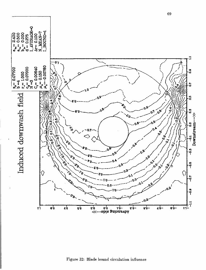
Figure 32: Blade bound circulation influence

70

Figure 33: Final choice of circulation first harmonic components

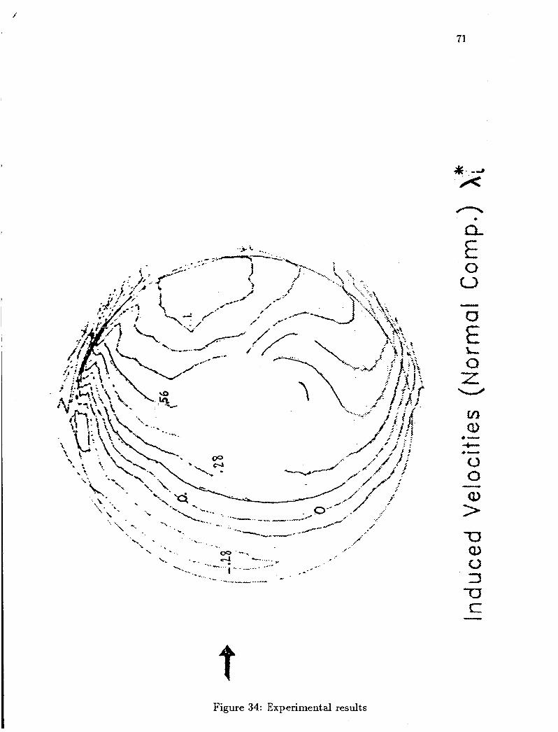
Figure 34: Experimental results

n

__- I

I I I I

ooro 9m'o OGO'O 920'0 000'0 GZ( '0- OGO'O- 9t&o'080T'O-

QJ 0

0

d! 0

m 0

c\! 0

~ U / A == 'y : opx M O I ~ pampq

Figure 35: Comparison computation-experiment at 0. degrees azimuth

73

r! -d

c\! -4

r! -4

9 -d

c? -0

CD -0 VJ

3 * d -0 E

4

E4 -0

u? -0

9 -0

@Y -0

c\! -0

OOT'O GLO'O OGOO GZO'O 000'0 GZO'O- OGO'O- ~L0'080T'O- ~ U / A = y : o y a MO~JUF pampq 1

Figure 36: Comparison computation-experiment at 30. degrees azimuth

74

ooro Sm'o OSO'O 920'0 000'0 920'0- 0900- SLO0-8O-rO- I grr/n = y : O ~ J M O I ~ pampq

Figure 37: Comparison computation-experiment at 60. degrees azimuth

75

a

OOT'O Gm'o OGO'O GZO'O 0000 GZO'O- OGO'O- Gc50'0-80T'O- 1 ~u/!A = y : o g x MOP pampq

Figure 38: Comparison computation-experiment at 90. degrees azimuth

c? -.--I

* -d

r! - 4

9 -d

e -0

m -0 a

4 -0

-0

u? -0

3 -0

n -0

c\! -0

OOT'O al0-0 OSiO'O S;ZO'O 0000 ZOO- 090'0- ~U) 'O-eOT'O- 1 ~ U / A = y : o p ~ M O I ~ pampq

Figure 39: Comparison computation-experiment at 120. degrees azimuth

77

OOT'O SL0.0 OGO'O SZO'O 000'0 SZO'O- 0900- So'o-8oro- 1 xcl/h = y : O J ~ . I MOIJUF pampq

Figure 40: Comparison computation-experiment at 150. degrees azimuth I

78

Td

OOT'O Sm'o OSiO'O 9ZO.O 000'0 GZO'O- OSO'O- %!J0'0*0T'O- ~ Q L A = y : o y a MOIJ~~T pampq 1

Figure 41: Comparison computation-experiment at 180. degrees azimuth

79

I I I I c?

1 rl I

OOT'O 9AO'O OGO'O 920'0 000'0 9zo.o- 0900- 9L50'0-80T'O- ~ U / A = 'y : O ~ J MOW pampq

Figure 42: Comparison computation-experiment at 210. degrees azimuth

80

-I---'

11 ll 1 0 0 I

00

-4

q -4

.-! -4

9 - 4

o! -0

m

-2 v) 3

-0

' 0

u? ' 0

9 '0

' 0

w '0

Figure 43: Comparison computation-experiment at 240. degrees azimuth

81

OOT'O sL0'0 OSO'O 9zo-0 000'0 szo*o- oso*o- sLOo430rO- ~ U / A = 'y : O ~ J MO~E pampq

Figure 44: Comparison computation-experiment at 270. degrees azimuth

82

I I

1

-+ I

I i I

OOT'O 9tLO'O 0900 9ZO.O 000'0 920'0- 090'0- 9r50'0-80T'O- ~ U / A = 1 y : O ~ J MO~E pampq

Figure 45: Comparison computation-experiment at 300. degrees azimuth

83

Figure 46: Comparison computation-experiment at 330. degrees azimuth

84

0 4

0

CD 0 0

cv 0 0

cv 0 0

I

CO 0 0 I

0

0 I

4

* = O =-NASA

* = SCULLY

0.4 .0.5 0.6 0.7 0.8 0.9 r/R

1

85

0 4 0

co. 0 0

02 0 r;

02 0 0 I

cf) 0 0 I

0

0 I

4

~~

.k = 30 = -NASA

* = SCULLY

0.4 .0.5 .0.6 0-8 0*9 1

Figure 48: Comparison Free-Wake and experiment at 30. degrees mimut,h

86

0 4

0

m 0 0

cv 0 0

02 0 0

I

m 0 0

I

0

0 I

4

0.4 0.5 .0.6

.k. = 60 =-NASA'

* = SCULLY

0.7

r/R 0.8 0.9 -1

Figure 49: Comparison. Free-Wake and experiment at 60. degrees azimuth

0 4

0

CD 0 0

cv 0 0

cv 0 0

I

CD 0 0

I

0 4 0

I

* = 90 =-NASA' = SCULLY

0.4 0.5 0.6 0.7 .0.8 0.9 1

Figure 50: Comparison Free-Wake and experiment at 90. degrees azimuth

88

0 4

0

a 0 0

cv 0 0

cv 0 0

I

CD 0 0

I

0 4 0

I 0.4 0.5

.\Ji- = 120 =-NASA = SCULLY

0.6 0.7 0.8 0*9 1

Figure 51: Comparison Free-Wake and experiment at 120. degrees azimuth

89

0 4

0

a 0 0'

cv 0 0

cv 0 0

I

a 0 0

I

0

0 I 4

0.4 0.5

9 = 150 =-NASAQ

* = SCULLY

0.6 0.7

r/R 0.8 0.9

Figure 52: Comparison Free-Wake and experiment, at 150. degrees azimuth

90

0 4 0 + = 180

9 =-NASA * = SCULLY

0.4 0.5 .0*6 0.7

r/R 0.8 0*9 1

Figure 53: Comparison Free-Wake and experiment at 180. degrees azimuth

91

0 4 0

CD 0 0

0.2 0 0

0 2 0 0

I

eo 0 0

I

0 4

0 I

~ .k= 210 = NASA

* = SCULLY

0.4 0.5 0.6 0.7 0.8 0.9 1

Figure 54: Coinparison Free-Wake and experiment at 210. degrees azimuth

92

0 4

0

00 H

U

0.4 .0.5

* = 240 =NASA

* = SCULLY

0.6 '0.7 0.8 -0.9 1

Figure 55: Comparison Free-Wake and experiment at. 240. degrees azimuth

0 4

0

a 0 0

cv 0 0.

N 0 0

I

CD 0 0

I

0

0 I 4

0.4 0.5

+ = 270 =.NASA- = SCULLY

0.6 0.7 0.8 0.9 1

Figure 56: Comparison Free-Wake and experiment at 270. degrees azimuth

.I . 94

0 7-l

0

co 0 0

0.2

a 0

cv 0 0

I

co 0 0

I

0

0 I

4

.\k = 300 =-NASAL

* = SCULLY

0.4 0.5 0.6 0.7 0.8 0.9 1

95

€3

0 L

z i H

W n

J

a 0 0

0.2 0 0

I

cz> 0 0

I

0 4

0

t3/ = 330 = NASA = SCULLY

1 I I I I I I I I I I

0.4 0.5 0.6 0.7

r/R 0.8 0.9 1