extremes: downscaling of percentiles and extremes events ... · date: 10/12/2013 clim-run...

Deliverable D3.7

© CLIM-RUN consortium

Date: 10/12/2013 CLIM-RUN (Dissemination Level PU) of 36

Collaborative Project

WP3 – Observational support and downscaling methods Task 3.2 Identification of parameters and indicators directly related to the key sectors

and target locations. Task 3.4 Downscaling methods and portal

Extremes: downscaling of percentiles and extremes events indicators

Project No. 265192– CLIM-RUN

Start date of project: 1st March 2011 Duration: 36 months Organization name of lead contractor for this deliverable: UEA

Due Date of Deliverable: August 2013 Actual Submission Date: December 2013

Authors: Richard Cornes, Clare Goodess, Ana Casanueva, Erika Coppola, Alessandro Dell’Aquila, Clotilde Dubois, M. Dolores Frías, Jose Manuel Gutiérrez, S. Herrera

Deliverable D3.7



Table of Contents 1. Introduction ....................................................................................... 3

2. Mediterranean analysis of temperature and precipitation extremes (UEA) ..................................................................................... 4

2.1 The CLIM-RUN common set of indices ............................................................ 4

2.2 Datasets and methods ...................................................................................... 4

2.3 Mediterranean-wide maps and Google Earth ................................................... 5

2.4 Case-study results for Greece, North Adriatic and Cyprus ............................... 6

2.5 Next steps ......................................................................................................... 8

3. Temperature and precipitation extremes in a multiple physics ensemble of RegCM4 (ICTP) ................................................................ 9

3.1 Indices, models and methods ........................................................................... 9

3.2. Key messages for CLIM-RUN stakeholders with respect to reliability and ‘skill’

................................................................................................................................ 9

3.3 Key messages for CLIM-RUN stakeholders with respect to past and future

changes ................................................................................................................ 11

3.4 Next steps ....................................................................................................... 13

4. Extreme precipitation in CNRM Med-CORDEX simulations (CNRM) ................................................................................................ 13

5. Statistical and dynamical downscaling of extreme temperature over Spain (UC) ................................................................................... 16

5.1 Data and Methods .......................................................................................... 16

5.2 Statistical downscaling .................................................................................... 17

6. Wind speed extremes (ENEA) ........................................................ 21

6.1 Data and methods .......................................................................................... 21

6.2 Main results .................................................................................................... 23

6.3 Summary ........................................................................................................ 28

7. Discussion and conclusions – some perspectives on Mediterranean extremes in the context of climate services ............ 28

References .......................................................................................... 30

Appendix ............................................................................................. 34

Deliverable D3.7



1. Introduction

Since many of the largest impacts of climate change on natural and human systems are likely to be due to changes in the frequency and intensity of extreme weather and climate events, it is not surprising that a strong demand for information about these events emerged from the first round of stakeholder workshops held in each of the CLIM-RUN case-study locations. In part, this demand was anticipated and the CLIM-RUN questionnaire produced by Workpackage 4 included questions concerning the current use of information about extremes as well as the desire for future predictions and projections for events such as heavy rainfall, frosts, heatwaves and very hot days/nights.

The emerging demands for information about extremes were consolidated during discussions between the CLIM-RUN Climate Expert Team and Stakeholder Expert Team and the wider WP2 and WP3 teams. One issue that emerged from the post-workshop discussions was that many different definitions of temperature and precipitation extremes had been used in the first round of workshops and sometimes the same name was used but with a different definition (e.g., different temperature thresholds were used to define hot days and tropical nights). Thus it was considered desirable to work, so far as possible, with a common set of definitions in order to avoid confusion both amongst the climate scientists and the stakeholders. It was also considered desirable to work with a relatively limited number of temperature and precipitation indices. Thus a common set of temperature and precipitation indices of extremes was identified and defined as described in milestone report M12 (see also Section 2 of this deliverable report). While many WP2 and WP3 partners have considered some aspects of extreme events, for example in the evaluation of the climate models they are using in CLIM-RUN, this deliverable provides an overview of the more specific and focused work that has been undertaken by five partners. In the majority of cases, this work has led, or is leading, to the production of specific climate products and related CLIM-RUN information sheets. Thus Section 2 describes work on temperature and precipitation extremes undertaken by UEA for the Mediterranean as a whole and for some selected case studies. Section 3 describes work undertaken by ICTP exploring uncertainties in a multiple physics ensemble. Section 4 considers the added value of the CNRM Med-CORDEX 12 km simulations particularly in the context of the Savoie tourism case study. Section 5 focuses on the evaluation of statistical downscaling of temperature extremes undertaken by UC using the statistical downscaling portal developed as part of CLIM-RUN Task 3.4. While the previous sections consider temperature and precipitation extremes, Section 6 describes work on extreme wind undertaken by ENEA. Finally, Section 7 provides some perspectives on Mediterranean extremes in the context of climate services, highlighting both science issues and issues relating to user needs. It should be noted that this deliverable focuses on climate projection timescales (i.e., the middle or end of the current century) rather than seasonal forecasts or decadal predictions. This is not because of the lack of interest or demand from users but rather a reflection of the current stage of development of such forecasts and predictions for the Mediterranean.

Deliverable D3.7



It should also be noted that CLIM-RUN work on more complex derived indices such as Fire Weather Indices (FWI) and various tourism comfort indices is reported elsewhere (for example, in Deliverable D3.4 on transfer functions. In some cases, results are shown for extreme values of these indices (e.g., in D3.5 some results relating to the 90th percentile of a statistically downscaled FWI are shown).

2. Mediterranean analysis of temperature and precipitation extremes (UEA)

2.1 The CLIM-RUN common set of indices The work done by WP4 in gathering together the stakeholders’ requirements formed the basis for the development of a common set of indices quantifying extremes of temperature and precipitation. Although the stakeholders’ comments ranged from a general interest in extremes to clear and specific requests, there was also considerable overlap in the requirements from many groups. As a result a common set of indices was identified, based primarily on the requirements of the stakeholders but also on the body of research over the last 20 years concerned with the development of indices of extremes based on daily data. The definitions were based on similar indices developed by the ETCCDI (http://etccdi.pacificclimate.org/) and STARDEX (http://www.cru.uea.ac.uk/cru/ research/ stardex/) projects. To balance the requirements of non-specialist stakeholders – who require the most relevant information presented in the simplest format – and the requirements of climate specialists – who require more information on the performance of the model runs – the indices were split into a core set (of most interest to stakeholders) and a supplementary set of indices (of additional importance to the Climate Expert Team). Details of the indices are provided in the Milestone 12 report of Work Package 3.

A further aim of these common indices has been to provide a Mediterranean-wide picture

of temperature and precipitation extremes. Within the CLIMRUN project there is a clear need for indices that have particular relevance to the case study sectors and areas themselves. However, indices that have meaning across the region have value in allowing the comparison of conditions for contrasting regions. In addition, some of the tourism stakeholders expressed an interest in knowing about potential changes in the source regions of tourists as well as in potential competing destination regions within the Mediterranean.

2.2 Datasets and methods The common set of indices (see Appendix) contains indices derived as percentile thresholds calculated from a base-period, and also those calculated as exceedances from fixed thresholds. Also included are duration-based indices (e.g. the Warm Spell Duration Index), which provide measures of the occurrence and persistence of spells of extreme conditions. Indices that compare values to base-period conditions (e.g. the number of days exceeding the 90th percentile) are calculated using the methods recommended by the ETCCDI (Zhang et al., 2011), with the 1971-2000 base-period used for all such indices. The indices were calculated from the E-OBS gridded dataset (V7.0, 0.25 x 0.25 degree resolution) (Haylock et al., 2008) and the RCM model-data (Table 2.1) developed by the

Deliverable D3.7



CIRCE project (Gualdi et al., 2012). The spatial resolutions of these models vary from 20-80 km. For the historic runs (1951-2000), observed greenhouse gases and aerosols have been used, and for the future runs (2001-2050) the forcing was achieved from the IPCC Special Report on Emissions Scenarios (SRES) A1B scenario. Note that the ENEA and MPI models are forced by the ECHAM5 and CMCC GCMs respectively, whereas the other models are fully coupled with the global ocean component listed in Table 2.1. All indices were calculated at the annual and standard three-month season resolutions.

Abbreviation Model Atmospheric Component

Global Ocean Component

Mediterranean Sea Component

INGV CMCC

(INGV)

ECHAM5

80 km, L31

OPA8.2-ORCA2

grid ~ 2° × 2°

(0.5° equator), L31

NEMO-MFS

1/16° (~7 km), L71

IPSL LMD

(IPSL version 3)

LMDZ global +

LMDZ regional

300 km, L19 +

30 km, L19

OPA9-ORCA2

~ 2° × 2°


NEMO-MED8

1/8° (9–12 km), L43

CNRM CNRM

(Météo-France/

CNRM)

ARPEGE-Climate

TL159c2.5,

stretched model:

50 km × 50 km

over Euro–

Mediterranean–

North Africa) L31

OPA9-ORCA2

~ 2° × 2°


NEMO-MED8

1/8° (9–12 km), L43

ENEA PROTHEUS

(ENEA)

RegCM3

30 km, L19

- MITgcm

1/8° (9–12 km), L42

MPI MPI

(MPI-HH)

REMO

25 km, L31

- MPI-OM

9 km, L29

Table 2.1. The Regional Circulation Models (RCMs) developed as part of the CIRCE project, and as used in this analysis. Adapted from Gualdi et al. (2012), and see references and details of abbreviations therein.

The extremes indices are also currently being calculated for the latest MED-CORDEX simulations (see Section 4) as the data become available. The MED-11 versions of these models have a much higher spatial resolution (12 km) than the CIRCE models and thus have the potential to provide more detail at the resolution typically required by stakeholders. The MED-CORDEX runs are also available at the coarser 40 km resolution, through which the added-value of the higher resolution data may be assessed. Thus indices are also being calculated for this coarser resolution data as well for two future emissions scenarios (RCP 4.5 and RCP 8.5).

2.3 Mediterranean-wide maps and Google Earth An archive of maps has been produced showing the results of the indices across the Mediterranean region. The maps show average conditions at the annual and seasonal resolutions for the following:

Average over the 1971-2000 baseline period

Deliverable D3.7



Average over the 2021-2050 scenario period

The difference in the averages between 1971-2000 and 2012-2050

The average difference over the 1971-2000 period between the model simulated results and the observed data (E-OBS)

The maps have been produced in Portable Network Graphics (PNG) and Google Earth formats. The latter format is considered to be particularly useful for stakeholders who will be able to analyse the results for their particular region of interest using software that is freely and widely available. An example of the Mediterranean-wide maps is provided in Figure 2.1, where the results of the average conditions 2021-2050 minus 1971-2000 are shown for the Warm Spell Duration Index (WSDI).

2.4 Case-study results for Greece, North Adriatic and Cyprus Although the extremes indices were calculated for the entire Mediterranean domain, values can easily be extracted for individual case-studies. Such data were extracted for the three case-study regions of Greece, North Adriatic and Cyprus, with the particular indices extracted being determined by the requirements of the individual regions:

Greece: HD, CDD, RX1day, RX5day

North Adriatic (Veneto/Friuli Venezia Giulia): WSDI, HD, RX1day, RX5day

Cyprus: HD, TR, CDDi, HDDi, CDD, RX5day

Figure 2.1. An example of the maps produced of the Mediterranean-wide extremes indices. This plot shows the difference in the average Warm Spell Duration Index (WSDI) for the period 2021-50 compared to 1971-2000. Each column shows the results for the CIRCE model data, with each row showing the results for the different seasons and year.

Deliverable D3.7



Maps ‘zoomed-in’ on these case-study regions were produced. In order to provide further local detail and context, the indices were also calculated from station data within the case study regions from the ECA&D archive, and in the case of the North Adriatic case study data from station data provided by the project's stakeholders (see Figure 2.2). In this example, for summer it is evident that neither E-OBS nor the models capture the lower-frequency

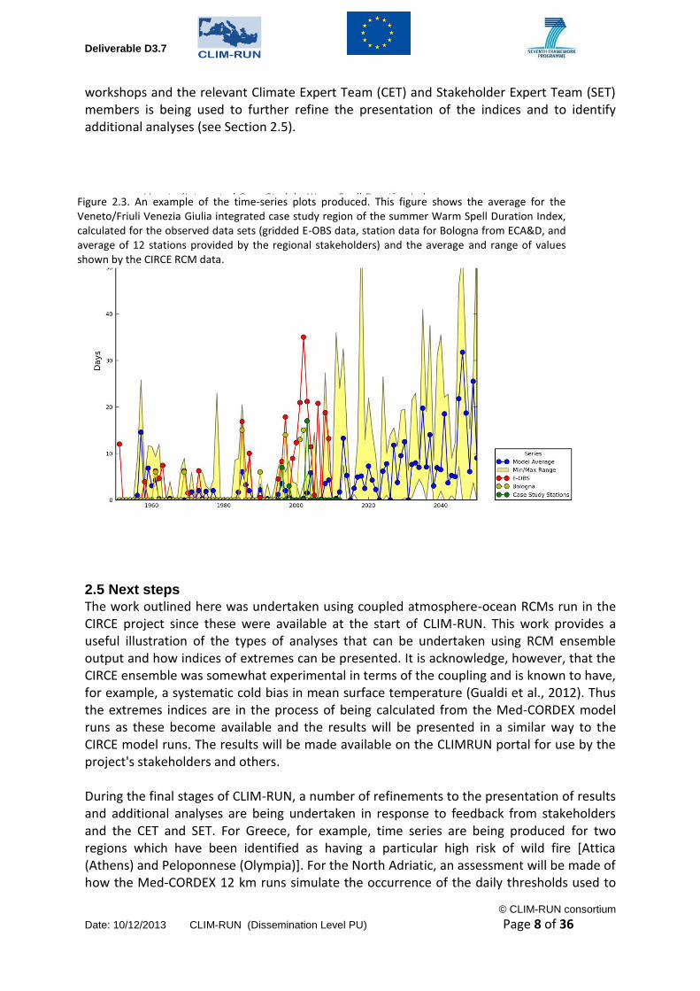
area around the Friuli Venezia Giuli plain. In addition to the temporal averages of the indices, spatial averages were constructed for the case study regions to produce time series plots (Figure 2.3). The simulated data in these cases were compared with the area averages from the gridded E-OBS data and also from individual stations in the respective case study regions. In the Figure 2.3 example, the RCMs reproduce WSDI fairly well in the first few decades, but underestimate the increased frequency of longer-lasting events over the most recent decade. All RCMs show a continuing increase: for 2021-2050 minus 2071-2100, the ensemble mean change is +10 days (model range is +3 days to +17 days). 2003 is a very extreme year in the observations and is not captured by the models, although they do simulate some very large events towards the middle of this century. The customized figures were presented at the second regional workshops for the case-study stakeholders, with the main features of the results being highlighted. These figures were presented with accompanying text highlighting issues such as the degree of correspondence between models and the observed data (both in terms of the magnitude of values and the direction of any trends), and the major features of the projections. Feedback from these

Figure 2.2. An example of the case-study-specific maps produced. This map shows the average of the number of hot days (HD) index for the period 1995-2012 as used by the Integrated Case Study. The results from the five CIRCE simulations are shown alongside the observed gridded data from E-OBS and the indices calculated from 83 station series supplied by one of the case-study’s project partners (VenFVG).

Deliverable D3.7



workshops and the relevant Climate Expert Team (CET) and Stakeholder Expert Team (SET) members is being used to further refine the presentation of the indices and to identify additional analyses (see Section 2.5).

2.5 Next steps

The work outlined here was undertaken using coupled atmosphere-ocean RCMs run in the CIRCE project since these were available at the start of CLIM-RUN. This work provides a useful illustration of the types of analyses that can be undertaken using RCM ensemble output and how indices of extremes can be presented. It is acknowledge, however, that the CIRCE ensemble was somewhat experimental in terms of the coupling and is known to have, for example, a systematic cold bias in mean surface temperature (Gualdi et al., 2012). Thus the extremes indices are in the process of being calculated from the Med-CORDEX model runs as these become available and the results will be presented in a similar way to the CIRCE model runs. The results will be made available on the CLIMRUN portal for use by the project's stakeholders and others. During the final stages of CLIM-RUN, a number of refinements to the presentation of results and additional analyses are being undertaken in response to feedback from stakeholders and the CET and SET. For Greece, for example, time series are being produced for two regions which have been identified as having a particular high risk of wild fire [Attica (Athens) and Peloponnese (Olympia)]. For the North Adriatic, an assessment will be made of how the Med-CORDEX 12 km runs simulate the occurrence of the daily thresholds used to

Figure 2.3. An example of the time-series plots produced. This figure shows the average for the Veneto/Friuli Venezia Giulia integrated case study region of the summer Warm Spell Duration Index, calculated for the observed data sets (gridded E-OBS data, station data for Bologna from ECA&D, and average of 12 stations provided by the regional stakeholders) and the average and range of values shown by the CIRCE RCM data.

Deliverable D3.7



define urban flooding within the region (58.4 mm if the previous 15 days are dry and 76 mm if precipitation occurs in the previous 15 days) and, if possible, an exploration of how the frequency of such events may change in the future. For Cyprus, UEA is also including WSDI and CDDi indices calculated from PRECIS model output for the Eastern Mediterranean provided by EEWRC. The case-study relevance of the CDDi data will be further enhanced by calculating cooling load using a simple formula provided by EEWRC. Information sheets will also be produced for each of these three case studies, as well as one for the Mediterranean-wide analysis of temperature and precipitation extremes.

3. Temperature and precipitation extremes in a multiple physics ensemble of RegCM4 (ICTP)

3.1 Indices, models and methods The ICTP model REgCM4 (Giorgi et al., 2012) was used to produce an ensemble of 50 km resolution simulations over the Mediterranean basin. The simulations cover the period 1970-2100 and they are driven by the greenhouse gas (GHG) concentration pathway RCP8.5. The ensemble members have different lateral and boundary conditions (from two GCMs: MPI and HadGEM), different land surface scheme (BATS; Dickinson et al., 1993 or CLM; Oleson et al., 2008) and different convection schemes (Grell, 1993; Emanuel and Zivkovic-Rothman, 1999). Three indices are used to measure the temperature and precipitation extremes:

Heat Wave Day Index (HWDI): Number of heat wave days, where a heat wave occurs when for at least Nd (five days were used here) consecutive days the daily maximum temperature exceeds the long term average by at least Nt (5° was used here) degrees.

Dry Spell Length Index (CDD): Maximum number of consecutive dry days, where a dry day is defined as having precipitation below 1 mm/day.

Heavy precipitation Index (R95): Percent of total precipitation above the 95% percentile

In Figures 3.1 and 3.2 the CDD and R95 maps are shown for five members of the ensemble (chosen as representative of the ensemble spread) and for the ensemble average (map highlighted in red). The TRMM VB42V46 (Huffman et al., 2007) observations are shown for comparison (map highlighted in blue).

3.2. Key messages for CLIM-RUN stakeholders with respect to reliability and ‘skill’

From Figures 3.1 and 3.2 the key message is that within an ensemble there can be some of the members that are outliers and the ensemble average is not always the best representation of the reality. In Figure 3.1, for example, the two ensemble members called HAdGEM CTRL 01 and 02 are closer to the observations in the Iberian Peninsula and in Northern France, but when they are averaged together with the other three members this

Deliverable D3.7



signal is lost and the ensemble average has a positive bias in these regions. Similar behaviour is observed in Figure 3.2 for the R95 index.

Figure 3.1. CDD climatology (number of days) for the reference period 1976-2005 for five RegCM4 ensemble members and for their ensemble average (red square). In the blue square the TRMM observations are shown for comparison.

Figure 3.2. R95 climatology (%) for the reference period 1976-2005 for five RegCM4 ensemble members and for their ensemble average (red square). In the blue square, the TRMM observations are shown for comparison.

Deliverable D3.7



3.3 Key messages for CLIM-RUN stakeholders with respect to past and future changes

In Figure 3.3 the past (1976-2006) and future (2071-2100) HWDI values are shown for the same five members and for their ensemble average (map highlighted in red). For both the present and future projections, the five members show an area of major disagreement in the projected magnitude of change in the Eastern part of Europe and around the Caspian Sea.

Figure 3.3. HWDI climatology (days) for the reference period 1976-2005 for five RegCM4 ensemble members and for their ensemble average (red square) (first and second columns from the left). HWDI climatology for the future period 2071-2100 for the same members and their ensemble average (third and fourth columns from the left).

In Figures 3.4 and 3.5 the change maps for CDD and R95 also show regions where the change signal (both in terms of magnitude and direction) is not shared by all the members, as for example the Balkan region, Turkey and the Caspian area. All these examples point toward the need of introducing a measure of uncertainty when the climate change signal is communicated to the stakeholders. Introducing a probability approach would be one possibility although the stakeholder community may dislike this (see Section 7).

Deliverable D3.7



Figure 3.4. Mean change (2071-2100 minus 1976-2005) in CDD (days) for five RegCM4 ensemble members and for their ensemble average (red square).

Figure 3.5. Mean change (2071-2100 minus 1976-2005) in R95 (%) for five RegCM4 ensemble members and for their ensemble average (red square).

Deliverable D3.7



3.4 Next steps The next steps would be to quantify for example the contributions to uncertainty of different factors, along with their synergy, in the regional climate model projections. This could be done by means of a Factor Separation method to assess the different sources of uncertainty in RCM-based regional climate projections.

4. Extreme precipitation in CNRM Med-CORDEX simulations (CNRM) The Mediterranean region is considered as a hot spot for climate change. The complex orography and its sharp coastline as well as the proximity of the Mediterranean sea requires high-resolution climate models to evaluate the impact of climate change in the region. Here, we focus on the representation of extreme precipitation using regional climate models. These models are tools to quantify the potential future change in precipitation. To evaluate the ability of regional climate models to reproduce extremes of precipitation we have performed simulations forced by ERA-Interim over the period 1979-2011. The simulations are performed at 12 and 50 km horizontal resolution. The performance of two models is evaluated: ALADIN-Climate developed at Météo-France (Colin et al., 2010) and COSMO-CLM developed at DWD (Rockel et al., 2008). These simulations are compared over the same period with observations from the SAFRAN gridded dataset over France (Vidal et al., 2010) which has a spatial resolution of 8 km.

Figure 4.1. (left) shows the representation of the 99% percentile or quantile in the ERA-Interim reanalysis in autumn. Precipitation values in this dataset reach 40-50 mm per day. These values are underestimated over large areas (the Alps, Pyrenees, Cevennes and Corsica) compared to the SAFRAN dataset ( right). In the SAFRAN observations, precipitation reaches extreme values of more than 100 mm per day in autumn.

Simulations over the period: 1989-2008 were performed using two regional climate models: ALADIN-Climate and COSMO-CLM at two different horizontal resolutions (50 and 12 km) forced by ERA-Interim at the lateral boundaries (Figures 4.2 and 4.3). The ability of these simulations to represent extreme precipitation in autumn in southern France has been assessed. As the spatial resolution increases, the spatial pattern of heavy precipitation is better represented and matches more the observations. Only at 12 km

Deliverable D3.7



resolution are the models able to represent the observed heavy precipitation (Figures 4.2 and 4.3) over the Pyrenees and Corsica and high values greater than 100 mm per day are reached.

Figure 4.2. 99% percentile for daily precipitation over the period 1989-2008 for COSMO-CLM forced by ERA-Interim reanalysis at 50 km (left) and 12 km (right) in autumn (SON).

Figure 4.3. 99% percentile for daily precipitation over the period 1989-2008 for ALADIN-Climate forced by ERA-Interim reanalysis at 50 km (left) and at 12 km (right) in autumn (SON).

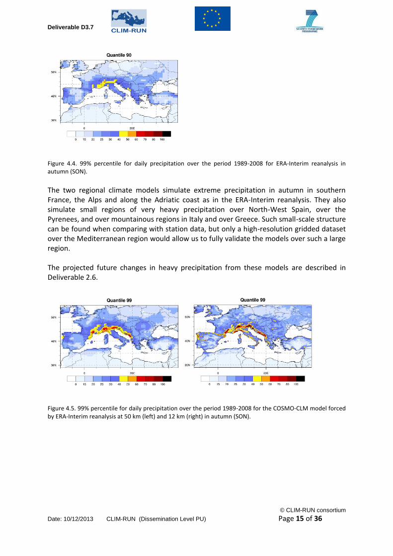
Such high resolution observed datasets as SAFRAN for validation are not available over the entire Mediterranean basin, but it is apparent that heavy precipitation over areas with strong orographic effects is better represented in simulations at higher spatial resolution. Thus we are looking at the representation of extreme rainfall over the whole Mediterranean region. Figure 4.4 shows extreme precipitation in autumn over the Mediterranean region for ERA-Interim over the period 1989-2008. Heavy precipitation is found over the Alps and along the Adriatic coast with the highest values reaching around 60 mm per day.

Deliverable D3.7



Figure 4.4. 99% percentile for daily precipitation over the period 1989-2008 for ERA-Interim reanalysis in autumn (SON).

The two regional climate models simulate extreme precipitation in autumn in southern France, the Alps and along the Adriatic coast as in the ERA-Interim reanalysis. They also simulate small regions of very heavy precipitation over North-West Spain, over the Pyrenees, and over mountainous regions in Italy and over Greece. Such small-scale structure can be found when comparing with station data, but only a high-resolution gridded dataset over the Mediterranean region would allow us to fully validate the models over such a large region. The projected future changes in heavy precipitation from these models are described in Deliverable 2.6.

Figure 4.5. 99% percentile for daily precipitation over the period 1989-2008 for the COSMO-CLM model forced by ERA-Interim reanalysis at 50 km (left) and 12 km (right) in autumn (SON).

Deliverable D3.7



Figure 4.6. 99% percentile for daily precipitation over the period 1989-2008 for the ALADIN-Climate model forced by ERA-Interim reanalysis at 50 km (left) and 12 km (right) in autumn (SON).

5. Statistical and dynamical downscaling of extreme temperature over Spain (UC)

Extremes are usually evaluated using extreme indicators (see Section 2 for example), based on statistics from the tails of the probability distribution function (typically percentiles). Some of these indices are based on the computation of high or low percentiles as reference, linking the lowest minimum temperatures to frost hazard risk and the highest maximum temperatures to heat stress conditions for example. In this study, we focus directly on the tail of the distribution of daily maximum and minimum temperatures analyzing high and low percentiles in daily maximum and minimum temperatures respectively. The study analyses the representation and future projection of these percentiles according to an ensemble of statistical downscaling methods over the Iberian Peninsula. More details about this study can be found in Casanueva et al. (2013) together with a comparison with dynamically downscaled results.

5.1 Data and Methods The high-resolution gridded data set Spain02 has been considered as reference observations to compare the downscaled results. Spain02 (Herrera, 2011, Herrera et al., 2012) is a freely available (http://www.meteo.unican.es/datasets/spain02) daily gridded precipitation and maximum and minimum temperature data set covering continental Spain and the Balearic Islands with 0.2° resolution. The interpolation of temperature is based on a large number of surface stations (thousands of stations), which have been selected using stringent quality control to cover the whole period (1950-2008) with few missing data. This data set is able to reproduce the intensity and spatial variability of the typical observed extremes. Although extremes are more sensitive to interpolation, the dense station coverage was crucial to get an accurate reproduction of these events. When evaluating extremes, it is of great importance to take into account the errors introduced by the observations used as reference. For instance, some studies using the state-of-the-art E-OBS gridded observational data set for Europe (Haylock et al., 2008, Hofstra et al., 2009) as reference data set to evaluate RCM results have reported that large model biases are found in regions with low station density (García-Díez et al., 2013,

Deliverable D3.7



Kjellstrom et al., 2010, Nikulin et al., 2011). Note that this problem is critical for extremes, since the actual extremes could be underestimated in the gridded observational data due to the interpolation process. To test the sensitivity of the downscaled results to the observational data set, we have also considered the E-OBS data set (version 5.0) developed within the EU-funded ENSEMBLES project for the period 1950-2010. The two different data sets (Spain02 and E-OBS) follow the same interpolation process for temperature, although the number of stations is higher in Spain02. A similar spatial distribution of high percentiles for maximum temperature (90th and 95th) and low percentiles for the minimum temperature (5th and 10th) over the Iberian Peninsula appears with both data sets, although E-OBS shows slightly lower values (figures not shown). Given the similarity of the percentile distribution we focus on the analysis of the 95th and 5th percentiles for maximum and minimum temperatures, respectively. Note that these percentiles are “extreme” in the sense that they sample the tails of the probability distribution. However, they are not associated with rare events, since their values are reached, on average, once every 20 days (i.e. more than four days per season) but note also that higher percentiles (e.g. 99th) would lead to unreliable estimates due to the small sample size.

5.2 Statistical downscaling

Data from different statistical downscaling methods (SD) are considered in this study. Statistical downscaling (SD) consists of building empirical models relating large-scale variables, which are well represented by Global Climate Models (GCMs), with local observations. The empirical model is then applied to future large-scale fields simulated by GCMs. The SD data used in this study were generated within the ESTCENA project (2008-2011), which aimed at generating regional climate change scenarios over Spain using SD methods (Gutiérrez et al., 2013). In particular, five SD methods were applied in this project: a non-linear analog method considering the euclidean distance to obtain a single nearest neighbor (S1, hereafter), three multiple linear regression methods considering the principal components (PCs) of the predictors explaining 95% of their variance up to a maximum of 30 PCs (S2), considering 15 PCs plus the nearest grid box values (S3), a combination of weather types (WTs) by k-means and the S3 method (S4) and, finally, a pure weather typing method (100 WTs) combined with a gaussian weather generator for each WT (S5). These five methods cover the statistical methodologies with the best results for the Iberian Peninsula according to Gutiérrez et al. (2013). Bear in mind that S2, S3 and S4 are connected since they are based on multiple regression models. Table 5.1 summarizes these methods and the variables considered as predictors in the downscaling. In most of the experiments sea level pressure (SLP) and daily mean temperature (T2m) were selected as predictors. The SD models were trained under perfect prog conditions using the ERA-40 reanalysis from the European Centre for Medium Range Weather Forecasts (Uppala et al., 2005) as large-scale predictor for the Spain02 surface predictands. The calibrated SD models were then applied to two GCMs, ECHAM5 and HADCM3Q0, considering the SRES A1B scenario.

Deliverable D3.7



Label G13 label Downscaling method Predictor Variables

S1 M1a Nearest neighbour (1 analogue) T2m and SLP

S2 M3a Linear regression with 30 PCs T2m and SLP

S3 M3c Linear regression with 15 PCs + Nearest grid box

T2m and SLP

S4 M4a S3 conditioned on 10 WTs (k-means) T2m (SLP for WT)

S5 M2c Gaussian on 100 WTs (k-means) T2m and SLP Table 5.1. Statistical downscaling methods and predictors. The second column is the label in Gutiérrez et al. (2013), which provides further details of the different methods.

The downscaling methods are first evaluated for present climate conditions, using reanalysis-driven simulations for the period 1971-2000. To this end, downscaled values from ERA-40 reanalysis (considered as “perfect” GCM output; (Brands et al., 2011)) are compared to the two reference observed data sets. Figure 5.1 shows the spatially averaged biases in summer (JJA) and winter (DJF) for the 5th (upper panels) and 95th (lower panels) percentiles using Spain02 (left) and E-OBS (right) reference datasets. This figure allows comparison of the biases of the different statistical downscaling methods, considering both the original and the unbiased downscaled values. Red lines in this plot correspond to the downscaling methods. The origin (the unlabeled end) of a line represents the seasonal biases in the percentile when no correction is applied. The end of each line (the labelled end) represents the biases when the seasonal mean bias is corrected. The lines corresponding to the reanalysis (blue) and to E-OBS (pink) are also depicted for reference. Finally, crosses at each end represent the spatial standard deviation of the biases.

Figure 5.1. Spatially averaged bias (in °C) of 5th percentile of daily minimum (upper panels) and 95th percentile of daily maximum (lower panels) temperature with respect to Spain02 (left panels) and E-OBS (right panels). Each panel is a cartesian (scatter) plot of the summer (JJA, Y axis) bias against the winter (DJF, X axis) one. The origin (the unlabeled end) of a line represents the seasonal biases in the percentile when no correction is applied. The end of each line (the labeled end) represents the biases when the seasonal mean bias is corrected. The line of each method is labeled according to Table 5.1 without the “S” initial for visual clarity. SD lines are depicted in red. The lines corresponding to the reanalysis (blue) and to E-OBS (pink) are also depicted for reference. Finally, crosses at each end represent the spatial standard deviation of the biases. For clarity, σ values are rescaled; the value σref=3°C is shown as reference.

Deliverable D3.7



Figure 5.2. Delta change values (in °C) averaged over the Iberian Peninsula for the period 2021-2050 of A1B scenario with respect to 1971-2000 of 20C3M. The origin (the unlabeled end) of a line represents delta values calculated for the mean values of minimum (left) and maximum (right) temperature in winter (DJF, X axis) and summer (JJA, Y axis). The end of the line (the labeled end) is the delta value for the 5th percentile (left) and the 95th percentile (right) for the daily minimum and maximum temperatures respectively. The line of each method is labeled according to Table 5.1; note that the “S” initial letter has been dropped for visual clarity. SD lines are depicted in red when they are nested in HADCM3Q0 and light red when they are nested in ECHAM5. Crosses indicate the standard deviation averaged over the Iberian Peninsula for winter (X axis) and summer (Y axis). σ are rescaled between 0 and 0.5, and the value σref =1°C is indicated in the legend as a reference.

For the statistical approaches (red crosses) both the mean biases and the spatial variability are larger in the E-OBS case, indicating that spatial variability is clearly affected by the baseline climate dataset used to fit/compare the empirical models. They change only slightly with the bias correction (except for the 95th percentile). Statistical methods seem to be separated into two clusters: one composed of methods based on linear regression S2-4 and a second cluster composed of S1 based on analogs and S5 based on a combination of a gaussian weather generator with the k-means weather typing. Moreover, for methods S2-4 the bias correction in the mean leads to larger biases in the percentiles, e.g. for the 95th percentile in winter. This indicates a good result for the wrong reason, probably caused by error cancellation between the mean and the variability of the statistically downscaled data using these methods. Results for the direct reanalysis output (blue line) show the largest bias, with slightly larger magnitudes and variability of results for E-OBS. The bias and the dispersion (blue crosses) also decrease with the correction in the seasonal mean. The pink line shows the biases (mean differences) from E-OBS with respect to Spain02. In the case of the 95th percentile the average difference over the Iberian Peninsula is 0.5°C, whereas it is negligible for the 5th percentile. These differences vanish when considering the bias corrected data. Figure 5.2 shows the spatially-averaged delta change values (and the spatial variability, represented by the crosses) over the Iberian Peninsula for the period 2021-2050. Colours of lines and labels are the same as in the previous cases. However, now the labelled end shows the delta values for the percentiles, whereas the unlabelled end indicates the delta for the mean values. The crosses represent the standard deviation of the increments over the

Deliverable D3.7



Iberian Peninsula which has been rescaled between 0 and 1°C, as shown in the figure. Values from the statistical downscaling methods are plotted in light red for those using the ECHAM5 GCM and dark red for those using the HADCM3Q0. The resulting values show an increase in both the mean and percentile values (note that the axes only show positive values). Higher values were found in the second period (2070-2099, not shown) for both the mean and the percentiles, in agreement with Fischer and Schar (2010). However, there is no consistent indication that the changes in percentiles are higher than changes in the mean; this varies from case to case, depending on the GCM or the downscaling approach. In general, changes are higher in summer than in winter for both percentiles. The increases for minimum temperatures in winter show more consistency among the different methods compared to the changes for maximum temperatures in summer. This result is in agreement with Hertig et al. (2010). The most notable result is the anomalous behaviour obtained for the statistical downscaling methods 1 and 5 (analogs and weather typing methods, see Table 5.1) for maximum temperature in summer. In this case, the methods are clear outliers with respect to the rest of the methodologies - particularly in the final period 2070-2099 (not shown), where the problem also affects the minimum temperature - due to a large underestimation of both the mean and percentile values, more pronounced in the latter case. This result is in agreement with Gutiérrez et al. (2013), where these two methods were reported to be non robust in climate change conditions, particularly for maximum temperature in summer, since they have no extrapolation capabilities. Our results show that this problem is even more pronounced for high/low percentiles. Apart from this anomalous behaviour, the results for the different GCM and downscaling method combinations for the near future period (2021-2050) cluster first according to the particular choice of GCM and, then, by the downscaling methods, with the variability of the different statistical downscaling methods contributing the smallest source of uncertainty. However, this does not hold by the end of the century (2070-2099) when the contribution to the total variability is shared similarly by all factors. Both in the near and far future periods, the differences between the percentiles and the mean temperature values are, in general, higher in summer than in winter and this is also the case for the spatial variability of the results. Finally, the spatial variability of the climate change signal (the delta) for the percentiles is of the same order as the error obtained when reproducing percentiles under perfect conditions, considering the case where the mean is corrected (note that the delta method implicitly performs an approximate cancellation of the mean). All of the above stresses the importance of considering an ensemble of different methodologies in the projection of future regional climate change. If a single method had been used in this study, the conclusions drawn regarding e.g. the relative increase of high/low temperature percentiles with respect to changes in the mean would be completely misleading, since they are method dependent. Techniques to identify non-robust downscaling methods, such as that proposed by Gutiérrez et al. (2013), are also key to understand ensembles of downscaled data, since such methods contribute to unrealistically increase regional climate change uncertainty. See Casanueva et al. (2013) for a comparison

Deliverable D3.7



of these statistical downscaled results with those from different dynamical downscaling models.

6. Wind speed extremes (ENEA)

Since the early stages of CLIM-RUN, wind speed has been clearly identified as one of the most relevant variables for stakeholders involved in different case studies. In particular, climate information about wind speed has been requested in the energy case study (Morocco and Cyprus), in the integrated case study for the North Adriatic region and for the wild fires case study (Greece). The capability of the Regional Climate Model (RCM) simulations produced during the ENSEMBLES project (Christensen et al., 2009) in representing climatological features of wind speed together with the projected changes in the seasonal averages of wind field has been already presented in Deliverable 2.4. However, the involved stakeholders are also interested in the changes of frequency and seasonality of strong wind events that can affect, for instance, wind power production (Marquis et al., 2011) as well as the propagation of wild fires. Even the description of days with very weak wind can be relevant in the framework of wind power production. Starting from the projected changes of wind speed at seasonal scale reported in Deliverable 2.4, here we analyse the corresponding changes in intense events over sites of interest in CLIM-RUN case studies along the Mediterranean coasts.

6.1 Data and methods

RCMs produce high-resolution (about 20 km) climate scenarios over selected areas by taking the input at the lateral boundaries from coarser resolution (about 100 km) Global Climate Models (GCMs). RCMs enhance the quality of climate projections with respect to GCMs, especially in the presence of complex orography (Artale et al., 2010) and in the proximity of coastal areas (Feser et al., 2011). In CLIM-RUN, we have evaluated wind modeling over the Euro-Mediterranean area using what is currently the largest and most consolidated ensemble of RCM simulations - produced during the EU-FP6 ENSEMBLES project (van der Linden and Mitchell 2009). Table 6.1 shows (in green) the GCM-RCM combinations that have been extracted from the ENSEMBLES archive to develop the CLIM-RUN products on intense wind events. We consider 15 1951-2050 SRES A1B scenario RCM simulations performed at a horizontal resolution of 25 km.

Deliverable D3.7



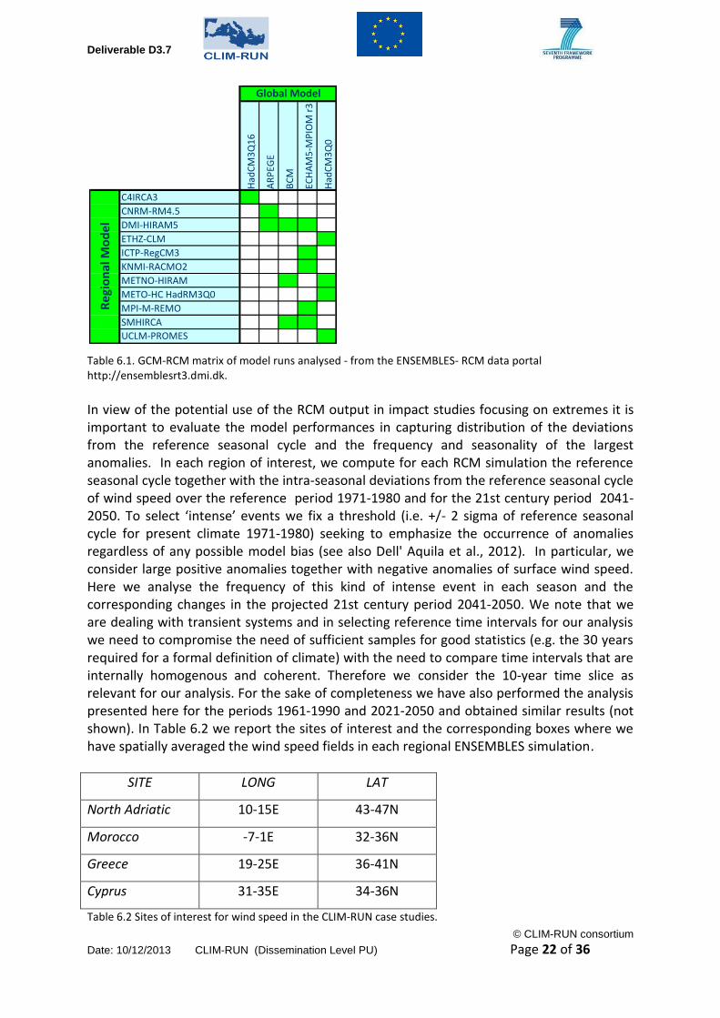
Table 6.1. GCM-RCM matrix of model runs analysed - from the ENSEMBLES- RCM data portal http://ensemblesrt3.dmi.dk.

In view of the potential use of the RCM output in impact studies focusing on extremes it is important to evaluate the model performances in capturing distribution of the deviations from the reference seasonal cycle and the frequency and seasonality of the largest anomalies. In each region of interest, we compute for each RCM simulation the reference seasonal cycle together with the intra-seasonal deviations from the reference seasonal cycle of wind speed over the reference period 1971-1980 and for the 21st century period 2041-2050. To select ‘intense’ events we fix a threshold (i.e. +/- 2 sigma of reference seasonal cycle for present climate 1971-1980) seeking to emphasize the occurrence of anomalies regardless of any possible model bias (see also Dell' Aquila et al., 2012). In particular, we consider large positive anomalies together with negative anomalies of surface wind speed. Here we analyse the frequency of this kind of intense event in each season and the corresponding changes in the projected 21st century period 2041-2050. We note that we are dealing with transient systems and in selecting reference time intervals for our analysis we need to compromise the need of sufficient samples for good statistics (e.g. the 30 years required for a formal definition of climate) with the need to compare time intervals that are internally homogenous and coherent. Therefore we consider the 10-year time slice as relevant for our analysis. For the sake of completeness we have also performed the analysis presented here for the periods 1961-1990 and 2021-2050 and obtained similar results (not shown). In Table 6.2 we report the sites of interest and the corresponding boxes where we have spatially averaged the wind speed fields in each regional ENSEMBLES simulation.

SITE LONG LAT

North Adriatic 10-15E 43-47N

Morocco -7-1E 32-36N

Greece 19-25E 36-41N

Cyprus 31-35E 34-36N

Table 6.2 Sites of interest for wind speed in the CLIM-RUN case studies.

Had

CM

3Q

16

AR

PEG

E

BC

M

ECH

AM

5-M

PIO

M r

3

Had

CM

3Q

0

C4IRCA3

CNRM-RM4.5

DMI-HIRAM5

ETHZ-CLM

ICTP-RegCM3

KNMI-RACMO2

METNO-HIRAM

METO-HC HadRM3Q0

MPI-M-REMO

SMHIRCA

UCLM-PROMES

Global ModelR

egi

on

al M

od

el

Deliverable D3.7



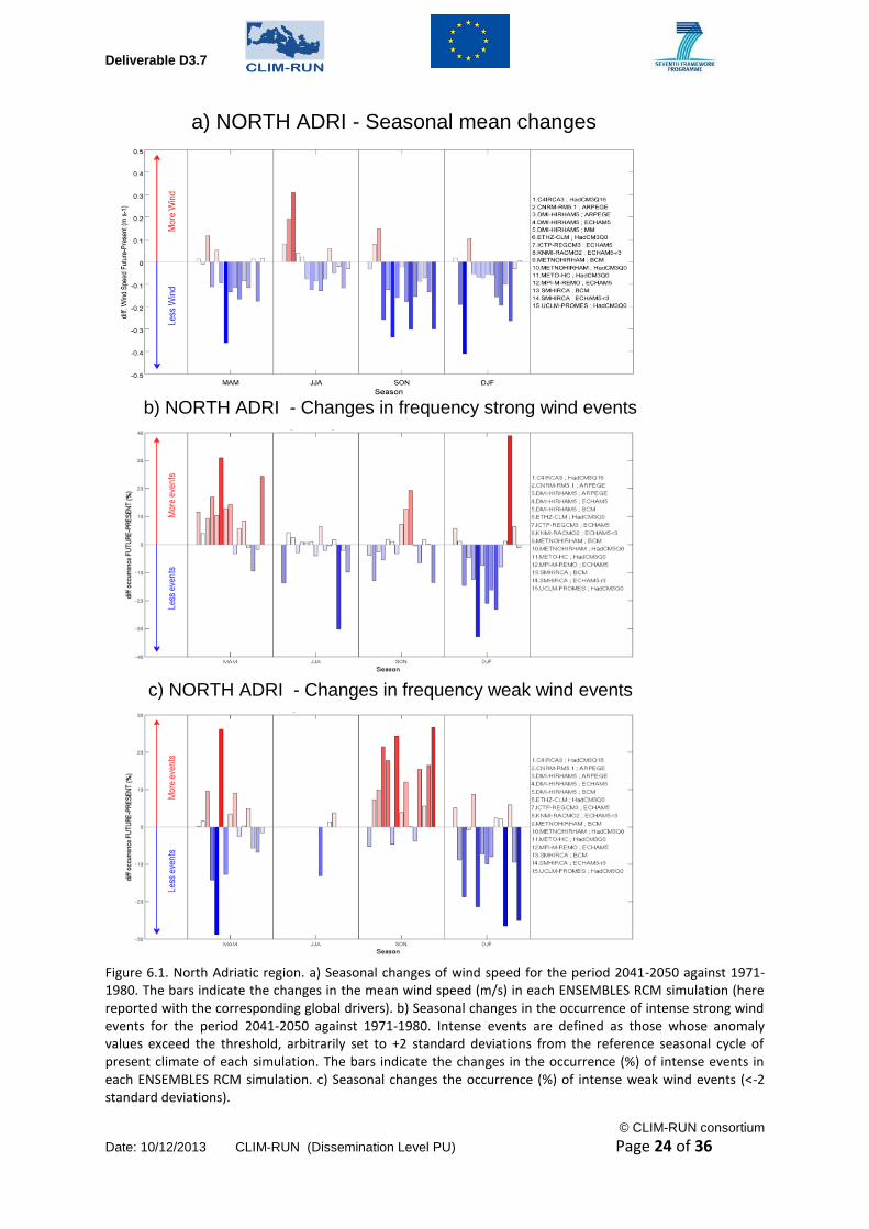
6.2 Main results The projected changes of wind speed for the North Adriatic region are shown in Figure 6.1. Figure 6.1a clearly highlights an overall decrease of seasonal averages of wind speed. Only a few simulations (mostly driven by ARPEGE) foresee a slight increase especially during summer. In this changed climatological mean state, Figure 6.1b show a strong increase (up to 30%) of large positive anomalies (i.e. strong windy events) especially during spring. During winter most of the analyzed simulations exhibit a significant decrease of these kind of events. Days characterized by large negative anomalies of wind speed (i.e. very weak wind) are projected to increase in the autumn season. Over Morocco (Figure 6.2a), the changes in wind speed seasonal averages are quite similar (even stronger) to those shown in Figure 6.1a for the North Adriatic but with an increased variability (more large anomalies with both signs) during winter. Over Greece a slight strengthening of wind speed is foreseen for summer (this could be particularly relevant for the wild fires case study), while in the other seasons weaker seasonal wind speed is expected. Regarding the representation of wind speed variability, the ENSEMBLES models do not agree - exhibiting a large spread of different behavior (Figure 6.3a-b). Similar conclusions can be drawn for Cyprus (Figure 6.4) where a general lowering of seasonal wind speed is expected for all seasons with a corresponding decrease of strong (and weak) wind events during winter.

Deliverable D3.7



Figure 6.1. North Adriatic region. a) Seasonal changes of wind speed for the period 2041-2050 against 1971-1980. The bars indicate the changes in the mean wind speed (m/s) in each ENSEMBLES RCM simulation (here reported with the corresponding global drivers). b) Seasonal changes in the occurrence of intense strong wind events for the period 2041-2050 against 1971-1980. Intense events are defined as those whose anomaly values exceed the threshold, arbitrarily set to +2 standard deviations from the reference seasonal cycle of present climate of each simulation. The bars indicate the changes in the occurrence (%) of intense events in each ENSEMBLES RCM simulation. c) Seasonal changes the occurrence (%) of intense weak wind events (<-2 standard deviations).

a) NORTH ADRI - Seasonal mean changes

b) NORTH ADRI - Changes in frequency strong wind events

c) NORTH ADRI - Changes in frequency weak wind events

Deliverable D3.7



Figure 6.2. As Figure 6.1 but for Morocco.

a) MOROCCO - Seasonal mean changes

b) MOROCCO - Changes in frequency strong wind events

c) MOROCCO - Changes in frequency weak wind events

Deliverable D3.7



Figure 6.3. As Figure 6.1 but for Greece.

a) GREECE - Seasonal mean changes

b) GREECE - Changes in frequency strong wind events

c) GREECE - Changes in frequency weak wind events

Deliverable D3.7



Figure 6.4. As Figure 6.1 but for Cyprus.

a) CYPRUS - Seasonal mean changes

b) CYPRUS - Changes in frequency strong wind events

c) CYPRUS - Changes in frequency weak wind events

Deliverable D3.7



6.3 Summary Here we have analysed the RCM simulations produced in the ENSEMBLES EU FP6 project in terms of their future projections regarding the major features of wind speed (seasonal averages together with large deviations from it) over some sites of interest for the CLIM-RUN project (North Adriatic, Morocco, Greece, Cyprus). This preliminary study should contribute to set a benchmark and present an impact-oriented methodology to be possibly applied to the new CORDEX simulations (in particular EURO-CORDEX and MED-CORDEX) where some additional validation analysis against observational datasets (e.g., QUIKSCAT) could also be performed (see also CLIM-RUN Deliverable 2.6).

7. Discussion and conclusions – some perspectives on Mediterranean extremes in the context of climate services There is an interest in having information about climate and weather extremes from all CLIM-RUN case studies and the analyses outlined in this deliverable indicate that the CLIM-RUN partners have gone some way to meeting these demands. However, as also reflected in the recent IPCC Special Report on Extremes (see in particular, Senerviratne et al., 2012) and the Fifth Assessment Report of Working Group I (see, for example, Table SPM.1 in the Summary for Policy Makers (IPCC, 2013)), the analysis of such events is complex due in large part to the high temporal and spatial resolutions which must be studied and because they are, by definition, rare (or at least relatively rare) events. Thus projection uncertainties, particularly for precipitation and wind extremes and with respect to the magnitude of change, tend to remain quite large. A number of common issues, relating both to the underlying climate science and to user needs and communication, have been identified during the course of the CLIM-RUN work on extremes and these are summarised below. Work will be done on some of these issues in the final stages of CLIM-RUN, but the issues listed below provide the basis for continuing work beyond the end of the project as well as guidance for future climate service related activities.

1. Climate science related issues a. The need for higher spatial resolution and exploration of its added value b. The need for bias correction c. Uncertainty and robustness of projections d. Availability of observed data

2. User needs and communication a. Is a common set of indices ‘useful’? b. Fixed vs percentile-based thresholds c. Return periods d. Other variables

In fact, the climate science and user issues are very much inter-related particularly in the context of communication. Section 3, for example, demonstrates some of the issues

Deliverable D3.7



relating to uncertainty and concludes that a probabilistic approach to projections would be desirable. Section 5 recommends the use of multiple statistical downscaling approaches as well as developing techniques to identify non-robust downscaling methods, in order to avoid unrealistic climate change signals. However, such approaches are rather at odds with the views expressed by forester stakeholders involved with the Greek wild fire case study, for example. These stakeholders were not interested in model validation but thought that climate scientists should choose the ‘most suitable’ model or just present the ensemble average. In this case, ways of simplifying the presentation for those who are completely unfamiliar with modelling – but still including some information about the range of projected change - are being explored. A number of the standard indices of extremes defined for CLIM-RUN are based on fixed-thresholds (35°C Tmax for Hot Days, 25°C Tmin for Tropical Nights, 25°C Taverage for Cooling degree days and 15°C Taverage for Heating degree days). Fixed thresholds were used due to the preferences expressed by stakeholders particularly in Greece and Cyprus. Yet the climate scientist’s preference is generally to work with percentile-based definitions. These are more meaningful when applied over larger geographic areas (the particular fixed thresholds used in the Mediterranean are not so applicable for Northern Europe, for example). There are also advantages in working with percentiles when models have biases. If model errors are systematic but the shape of the observed distribution is reasonably well simulated, then using percentiles helps to ‘correct’ for biases (if the percentile thresholds used for analysing model output are calculated from the model output itself). It is apparent that the models used in CLIM-RUN are subject to biases compared with observed extremes (see Figure 2.2 for example) and these biases sometimes differ from those found for mean temperature and precipitation. Cold biases in the CIRCE models are complicating the analysis of CDDi and HDDi for some countries being undertaken by UEA as input to part of the Task 4.4 IPTS economic modelling work. This highlights the necessity of developing and applying robust and reliable bias correction methods. Some preliminary work has been done by UEA on defining the specific requirements of bias correction methods and on the identification of appropriate methods and how to evaluate them including their effect on extreme values. While in general it is considered that it has been helpful to both climate scientists and stakeholders to work with a common set of indices of extremes, it is apparent that these are not appropriate in all situations and do not meet all needs. The 35°C Tmax threshold used to define Hot Days is, for example, currently exceeded on the majority of summer days at Larnaca and Nicosia in Cyprus, so cannot be considered ‘extreme’ for these locations. The common set of indices was chosen to have some relevance for impacts. This is most evident in the inclusion of heating and cooling degree day indices. The maximum one day and five day precipitation indices were chosen since they should have some relevance for the risk of flooding in smaller and larger catchments respectively. In practice, however, flood risk is generally defined using more locally tailored definitions. In the Veneto region, for example, the daily precipitation threshold used to define the risk of urban flooding is 58.4 mm if the previous 15 days are dry and 76 mm if precipitation occurs in the previous 15 days. This particular definition highlights the importance of precedent conditions in terms of impacts. Yet there is a lack of studies and indices for exploring sequences of events, compound or

Deliverable D3.7



combined events, and clustering of events in space or time (Goodess et al., 2012). The CLIM-RUN standard set of indices does not include return period estimates although in later stages of CLIM-RUN a few stakeholders expressed an interest in these. The availability of suitable observed data has been a constraint for many of the CLIM-RUN analyses. The E-OBS gridded dataset has been used by several groups but discrepancies have been noted for Spain where comparison with the Spain-02 dataset based on considerably higher station density is possible (see Section 5). While area-averaged extreme values are always expected to be lower in magnitude than point values (Haylock et al., 2008), the large differences between E-OBS and station-based temperature extremes for Cyprus indicates issues with the gridded data for this small island location. In this particular example, it is however, reassuring that the observed and simulated trends are generally consistent and projected to continue to the middle of the century. Uncertainty in observational datasets is being increasingly recognised as a source of uncertainty in climate model evaluation. E-OBS has a spatial resolution of 25 km and thus alternative datasets must be used for evaluation of the new 12 km MED-CORDEX model runs (see Section 4). While the preliminary analysis presented in Section 4 indicates added value in areas with strong orographic effects, this can only be rigorously demonstrated for France for which an appropriate high-resolution data set (SAFRAN at 8 km) is available. Furthermore E-OBS only provides daily temperature and precipitation so other datasets must be used to evaluate variables such as wind (see Section 6). The analyses presented here focus on temperature and precipitation extremes (Sections 2 to 5), with one considering wind extremes (Section 6). Within the constraints of the project resources, it has not been possible to address some of the other types of events of interest to a few case-study stakeholders. These include storms, storm surges and dust storms.

References

Artale, V., Calmanti, S., Carillo, A., Dell’aquila, A., Herrmann, M., Pisacane, G., Ruti, P., Sannino, G., Struglia, M., Giorgi, F., Bi, X., Pal, J. & Rauscher, S. 2010. An atmosphere–ocean regional climate model for the Mediterranean area: assessment of a present climate simulation. Climate Dynamics, 35, 721-740.'10.1007/s00382-009-0691-8:' 10.1007/s00382-009-0691-8

Brands, S., Gutiérrez, J. M., Herrera, S. & Cofiño, A. S. 2011. On the Use of Reanalysis Data for Downscaling. Journal of Climate, 25, 2517-2526.'10.1175/jcli-d-11-00251.1:' 10.1175/jcli-d-11-00251.1

Casanueva, A., Herrera, S., Fernandez, J., Frias, M. D. & Gutierrez, J. M. 2013. Evaluation and projection of daily temperature percentiles from statistical and dynamical downscaling methods. Natural Hazards and Earth System Sciences, 13, 2089-2099.'DOI 10.5194/nhess-13-2089-2013:' DOI 10.5194/nhess-13-2089-2013

Christensen, J., Rummukainen, M. & Lenderink, G. 2009. Formulation of very-high-resolution regional climate model ensembles for Europe. In: VAN DER LINDEN, P. & MITCHELL, J. F. B. (eds.) ENSEMBLES: Climate Change and

Deliverable D3.7



its Impacts: Summary of research and results from the ENSEMBLES project. Met Office Hadley Centre, FitzRoy Road, Exeter EX1 3PB, UK.

Colin, J., Déqué, M., Radu, R. & Somot, S. 2010. Sensitivity study of heavy precipitation in Limited Area Model climate simulations: influence of the size of the domain and the use of the spectral nudging technique. Tellus A, 62, 591-604.'10.1111/j.1600-0870.2010.00467.x:' 10.1111/j.1600-0870.2010.00467.x

Dell' Aquila, A., Calmanti, S., Ruti, P., Struglia, M. V., Pisacane, G., Carillo, A. & Sannino, G. 2012. Effects of seasonal cycle fluctuations in an A1B scenario over the Euro-Mediterranean region. Climate Research, 52, 135-157.'10.3354/cr01037:' 10.3354/cr01037

Dickinson, R.E., Henderson-Sellers, A. & Kennedy, P.J. 1993. Biosphere – Atmosphere Transfer Scheme, BATS: version 1E as coupled to the NCAR Community Climate Model. Technical Note NCAR/TN – 387 + STR, 72p.

Emanuel, K.A. & Zivkovic-Rothman, M. 1999. Development and evaluation of a convection scheme for use in climate models. Journal of Atmospheric Science, 56, 1766–1782.

Feser, F., Rockel, B., Von Storch, H., Winterfeldt, J. & Zahn, M. 2011. Regional Climate Models Add Value to Global Model Data: A Review and Selected Examples. Bulletin of the American Meteorological Society, 92, 1181-1192.'10.1175/2011bams3061.1:' 10.1175/2011bams3061.1

Fischer, E. M. & Schar, C. 2010. Consistent geographical patterns of changes in high-impact European heatwaves. Nature Geoscience, 3, 398-403.'Doi 10.1038/Ngeo866:' Doi 10.1038/Ngeo866

García-Díez, M., Fernández, J., Fita, L. & Yagüe, C. 2013. Seasonal dependence of WRF model biases and sensitivity to PBL schemes over Europe. Quarterly Journal of the Royal Meteorological Society, 139, 501-514.'10.1002/qj.1976:' 10.1002/qj.1976

Giorgi, F. et al. 2012. RegCM4: Model description and preliminary tests over multiple CORDEX domains. Climate Research, 52, 7−29.

Goodess, C.M. 2012. How is the frequency, location and severity of extreme events likely to change up to 2060? Environmental Science and Policy, http://dx.doi.org/10.1016/j.envsci.2012.04.001.

Grell, G.A. 1993. Prognostic evaluation of assumptions used by cumulus parameterizations. Monthly Weather Review, 121, 764–787.

Gualdi, S., Somot, S., Li, L., Artale, V., Adani, M., Bellucci, A., Braun, A., Calmanti, S., Carillo, A., Dell'aquila, A., Déqué, M., Dubois, C., Elizalde, A., Harzallah, A., Jacob, D., L'hévéder, B., May, W., Oddo, P., Ruti, P., Sanna, A., Sannino, G., Scoccimarro, E., Sevault, F. & Navarra, A. 2012. The CIRCE Simulations: Regional Climate Change Projections with Realistic Representation of the Mediterranean Sea. Bulletin of the American Meteorological Society, 94, 65-81.'10.1175/bams-d-11-00136.1:' 10.1175/bams-d-11-00136.1

Gutiérrez, J. M., San-Martín, D., Brands, S., Manzanas, R. & Herrera, S. 2013. Reassessing Statistical Downscaling Techniques for Their Robust Application under Climate Change Conditions. Journal of Climate, 26, 171-188.'10.1175/jcli-d-11-00687.1:' 10.1175/jcli-d-11-00687.1

Haylock, M. R., Hofstra, N., Klein Tank, A. M. G., Klok, E. J., Jones, P. D. & New, M. 2008. A European daily high-resolution gridded data set of surface temperature and precipitation for 1950–2006. Journal of Geophysical Research: Atmospheres, 113, D20119.'10.1029/2008jd010201:' 10.1029/2008jd010201

Deliverable D3.7



Herrera, S. 2011. Desarrollo, validación y aplicaciones de Spain02: Una rejilla de alta resolución de observaciones interpoladas para precipitación y temperatura en España. Universidad de Cantabria.

Herrera, S., Gutiérrez, J. M., Ancell, R., Pons, M. R., Frías, M. D. & Fernández, J. 2012. Development and analysis of a 50-year high-resolution daily gridded precipitation dataset over Spain (Spain02). International Journal of Climatology, 32, 74-85.'10.1002/joc.2256:' 10.1002/joc.2256

Hertig, E., Seubert, S. & Jacobeit, J. 2010. Temperature extremes in the Mediterranean area: trends in the past and assessments for the future. Natural Hazards and Earth System Sciences, 10, 2039-2050.'DOI 10.5194/nhess-10-2039-2010:' DOI 10.5194/nhess-10-2039-2010

Hofstra, N., Haylock, M., New, M. & Jones, P. D. 2009. Testing E-OBS European high-resolution gridded data set of daily precipitation and surface temperature. Journal of Geophysical Research: Atmospheres, 114, D21101.'10.1029/2009jd011799:' 10.1029/2009jd011799

Huffman, G.J. et al. 2007. The TRMM multisatellite precipitation analysis (TMPA): Quasi-global, multiyear, combined-sensor precipitation estimates at fine scale. Journal of Hydrometeorology, 8, 38-55.

IPCC 2013. Summary for Policymakers. In: Stocker, T. F., Qin, D., Plattner, G.-K., Tignor, M., Allen, S. K., Boschung, J., Nauels, A., Xia, Y., Bex, V. & Midgley, P. M. (eds.) Climate Change 2013: The Physical Science Basis. Contribution of Working Group I to the Fifth Assessment Report of the Intergovernmental Panel on Climate Change. Cambridge, United Kingdom and New York, NY, USA: Cambridge University Press.

Kjellstrom, E., Boberg, F., Castro, M., Christensen, H., Nikulin, G. & Sanchez, E. 2010. Daily and monthly temperature and precipitation statistics as performance indicators for regional climate models. Climate Research, 44, 135-150.'10.3354/cr00932:' 10.3354/cr00932

Marquis, M., Wilczak, J., Ahlstrom, M., Sharp, J., Stern, A., Smith, J. C. & Calvert, S. 2011. Forecasting the Wind to Reach Significant Penetration Levels of Wind Energy. Bulletin of the American Meteorological Society, 92, 1159-1171.'10.1175/2011bams3033.1:' 10.1175/2011bams3033.1

Nikulin, G., Kjellstrom, E., Hansson, U. L. F., Strandberg, G. & Ullerstig, A. 2011. Evaluation and future projections of temperature, precipitation and wind extremes over Europe in an ensemble of regional climate simulations. Tellus A, 63, 41-55.'10.1111/j.1600-0870.2010.00466.x:' 10.1111/j.1600-0870.2010.00466.x

Oleson, K. et al. 2008. Improvements to the community land model and their impact on the hydrological cycle. Journal of Geophysical Research, 113, G01021, doi:10.1029/2007JG000563.

Rockel, B., Will, A. & Hense, A. 2008. The Regional Climate Model COSMO-CLM(CCLM). Meteorologische Zeitschrift, 17, 347-348.'10.1127/0941-2948/2008/0309:' 10.1127/0941-2948/2008/0309

Seneviratne, S.I., Nicholls, N., Easterling, D., Goodess, C.M., Kanae, S., Kossin, J., Luo, Y., Marengo, J., McInnes, K., Rahimi, M., Reichstein, M., Sorteberg, A., Vera, C. & Zhang, X. 2012. Changes in climate extremes and their impacts on the natural physical environment. In: Managing the Risks of Extreme Events and Disasters to Advance Climate Change Adaptation. A Special Report of Working Groups I and II of the Intergovernmental Panel on Climate Change [Fields, C.B., V. Barros, T.F. Stocker, D. Qin, D.J. Dokken, K.L. Ebi, M.D.

Deliverable D3.7



Mastrandrea, K.J. Mach, G.-K. Plattner, S.K. Allen, M. Tignor and P.M. Midgley (eds.)]. Cambridge University Press, Cambirdge, UK, and New York, NY, USA, pp 109-230

Uppala, S. M., Kållberg, P. W., Simmons, A. J., Andrae, U., Bechtold, V. D. C., Fiorino, M., Gibson, J. K., Haseler, J., Hernandez, A., Kelly, G. A., Li, X., Onogi, K., Saarinen, S., Sokka, N., Allan, R. P., Andersson, E., Arpe, K., Balmaseda, M. A., Beljaars, A. C. M., Berg, L. V. D., Bidlot, J., Bormann, N., Caires, S., Chevallier, F., Dethof, A., Dragosavac, M., Fisher, M., Fuentes, M., Hagemann, S., Hólm, E., Hoskins, B. J., Isaksen, L., Janssen, P. a. E. M., Jenne, R., Mcnally, A. P., Mahfouf, J. F., Morcrette, J. J., Rayner, N. A., Saunders, R. W., Simon, P., Sterl, A., Trenberth, K. E., Untch, A., Vasiljevic, D., Viterbo, P. & Woollen, J. 2005. The ERA-40 re-analysis. Quarterly Journal of the Royal Meteorological Society, 131, 2961-3012.'10.1256/qj.04.176:' 10.1256/qj.04.176

Van Der Linden, P. & Mitchell , J. F. B. 2009. ENSEMBLES: Climate Change and its Impacts: Summary of research and results from the ENSEMBLES project. Met Office Hadley Centre, FitzRoy Road, Exeter EX1 3PB, UK. :

Vidal, J.-P., Martin, E., Franchistéguy, L., Baillon, M. & Soubeyroux, J.-M. 2010. A 50-year high-resolution atmospheric reanalysis over France with the Safran system. International Journal of Climatology, 30, 1627-1644.'10.1002/joc.2003:' 10.1002/joc.2003

Zhang, X., Alexander, L., Hegerl, G. C., Jones, P., Tank, A. K., Peterson, T. C., Trewin, B. & Zwiers, F. W. 2011. Indices for monitoring changes in extremes based on daily temperature and precipitation data. Wiley Interdisciplinary Reviews: Climate Change, 2, 851-870.'10.1002/wcc.147:' 10.1002/wcc.147

Deliverable D3.7



Appendix

The definitions of the standard set of extremes indices used in Section 2. Reproduced from the Milestone 12 report. Daily Temperature Extremes

Core Indices

Code

Name

Derivation Notes

Intensity-related impact indices

CDDi Cooling degree-days Sum of Tg-25°C, for all Tg>25°C

Model data will likely need bias correction.

HDDi Heating degree-days Sum of 15°C -Tg, for all Tg<15°C

-ditto-

Frequency-related indices

TN90n Warm nights Number of days with TN exceeding TN90p

Thresholds constructed using the ETCCDI method

TN10n Cold nights Number of days with TN falling below TN10p

-ditto-

TX90n Warm days Number of days with TX exceeding TX90p

-ditto-

TX5n Cold days Number of days with TX falling below TX10p

-ditto-

CDDn Cooling degree-day frequency Number of days where CDD > 5

See CDD definition above

HDDn Heating degree-day frequency Number of days where HDD > 5

See HDD definition above

TR25 Tropical Nights Number of days where TN > 25°C

Model data will likely need bias correction.

HD Hot Days Number of days where TX > 35°C

-ditto-

Duration-related indices

WSDI Warm-spell duration index Sum of days in a span of ≥ 6 days where TX > 90th percentile.

Thresholds constructed using the ETCCDI method

CSDI Cold-spell duration index Sum of days in a span of ≥ 6 days where TN < 10th percentile

-ditto-

Supplementary Indices

Code

Name

Derivation

Notes

Intensity-related indices

Deliverable D3.7



TN10p Cold night threshold 10th percentile of TN Thresholds constructed using the ETCCDI method

TN90p Warm night threshold 90th percentile of TN -ditto-

TX10p Cold day threshold 10th percentile of TX -ditto-

TX90p Warm day threshold 90th percentile of TX -ditto-

Indices of Daily Precipitation Extremes

Core Indices

Code

Name Derivation

Notes


RX1day Highest 1-day rainfall Highest rainfall amount in one-day period

RX5day Highest 5-day rainfall Highest rainfall amount in five-day period

R95pTOT Precipitation on very wet days Total of rainfall from days when RR>R95p


R10mm

Heavy precipitation days

Count of days where RR ≥ 10mm.

Duration-related indices

CDD Consecutive dry days Maximum length of dry spell (RR < 1 mm).

CWD Consecutive wet days Maximum length of wet spell (RR ≥ 1 mm)

Supplementary Indices

Code

Name

Derivation

Notes


P95p Very wet day threshold 95th percentile of RR

Deliverable D3.7



SDII Simple daily intensity index Mean of precipitation on days when rain occurred (days when RR ≥ 1mm).


R20mm

Very heavy precipitation days

Count of days where RR (daily precipitation amount) ≥ 20mm.

extremes: downscaling of percentiles and extremes events ... · date: 10/12/2013 clim-run...

Documents