i

EXTREME TRADING VOLUME

AND EXPECTED RETURN

Study to Companies Listed in Indonesia Stock Exchange 2008-2012 Period

BACHELOR THESIS

Submitted as a requirement to complete Bachelor Degree (S1) at Bachelor

Program of Faculty of Economics and Business Diponegoro University.

Written by:

NOVITA INDAH NUGRAHENI

NIM. C2A008116

FACULTY OF ECONOMICS AND BUSINESS

DIPONEGORO UNIVERSITY

SEMARANG

2013

i

APPROVAL

Author : Novita Indah Nugraheni

Student ID : C2A 008 116

Faculty/Major : Economics and Business/Management

Title : EXTREME TRADING VOLUME AND EXPECTED

RETURN (STUDY TO COMPANIES LISTED IN

INDONESIA STOCK EXCHANGE 2008-2012 PERIOD)

Paper Advisor : Drs. H. Prasetiono, M.Si

Semarang, July 18th

, 2013

Paper Advisor

Drs. H. Prasetiono, M.Si

NIP. 196003141986031005

ii

APPROVAL

Author : Novita Indah Nugraheni

Student ID : C2A 008 116

Faculty/Major : Economics and Business/Management

Title : EXTREME TRADING VOLUME AND EXPECTED

RETURN (STUDY TO COMPANIES LISTED IN

INDONESIA STOCK EXCHANGE 2008-2012 PERIOD)

Has passed the examination on July 23rd

, 2013

Examiners:

1. Drs. H. Prasetiono, M.Si (...................................................)

2. Erman Denny Arfinto, S.E, M.M (...................................................)

3. Dr. Harjum Muharram, S.E, M.E (...................................................)

iii

BACHELOR THESIS ORIGINALITY STATEMENT

I am who undersigned here, Novita Indah Nugraheni, claimed that

bachelor thesis entitled Extreme Trading Volume and Expected Return (Study to

Companies Listed in Indonesia Stock Exchange 2008-2012 Period) is my own

writing. Hereby I declare in truth that this bachelor thesis there is no other’s

writings as a whole or as a part which I took by copy or imitate in a form of

sentences or symbol which represent writer’s ideas or opinions, which I admitted

as my own, and/or there is no a part or a whole writing which I copied, or I took

from other’s writings, without giving consent to its original writer.

Hereby I declare if I took action contrary to the matters above, whether it’s

on purpose or not, I will take back my proposed bachelor thesis which I admitted

as my own. Later on if it’s proved that I copied or imitated other’s writing as if it

was mine, I’ll let my academic title and certificate which has given to me to be

invalidated.

Semarang, 15 July 2013

Undersigned,

Novita Indah Nugraheni

NIM. C2A 008 116

iv

MOTTO

“Allah does not charge a soul except (with that within) its capacity. It will have

(the consequence of) what (good) it has gained, and it will bear (the consequence

of) what (evil) it has earned. "Our Lord, do not impose blame upon us if we have

forgotten or erred. Our Lord, and lay not upon us a burden like that which You

laid upon those before us. Our Lord, and burden us not with that which we have

no ability to bear. And pardon us; and forgive us; and have mercy upon us. You

are our protector, so give us victory over the disbelieving people."

“My dream isn’t to be ‘the best’, it’s to be someone who I’m not ashamed to be. I

believe if I don’t give up my hopes and dreams, then there will always be a good

ending.”

“I dedicated this for you, Ibu, Ayah, and the whole family.

I’m so grateful for everything. I’ll always work hard

to be the daughter you proud of”

v

ACKNOWLEDGEMENT

All praise and gratefulness to Allah SWT, because only with His mercy

and grace, the thesis with title “Extreme Trading Volume and Expected Return.

Study to Companies Listed in Indonesia Stock Exchange 2008-2012 Period” has

finally accomplished.

This thesis is a final assignment for Bachelor Program, Management

Department, Finance Management Major, Faculty of Economics and Business,

Diponegoro University. During the making of this thesis, I have received many

helps and endless support from many people in which I really grateful of. In form

of my gratefulness and appreciation, I would like to say my gratitude to:

1. Prof. Drs. H. Mohammad Nasir, M.S.i, Akt, PhD as the Dean of Faculty of

Economics and Business Diponegoro University, Semarang, which has

allowed me to write this thesis.

2. Drs. H. Prasetiono, M.Si as counselor which has gave me directions,

advices, and guidance throughout the making of this thesis.

3. Idris, SE, M.Si as the trustee which gave me all helps during my study and

the making of this thesis.

4. Erman Denny Arfinto, SE, MM as the exceptional lecturer I’ve assisted

for the past years who always give me unconditional supports.

5. All lecturers and employees in Faculty of Economics and Business

Diponegoro University, for all the given knowledges and supports during

my time.

vi

6. Mom, Dad, my brother, and the whole family which has given endless

support and encouragements.

7. My dependable friends; Indri, Anggun, Ade, Rizky, Dimas Adi, Dimas

Langgeng, Eko, Cahaya, Dery, Dito, Adit, Vidya, Niken, Amri, Dhiar,

Danu, Whisnu, Erisa, Anis, Endri, and Cicik. See you guys on top.

8. All my comrades in Management 2008, Management squad and FEB as

whole, seniors and juniors. Thanks for all the good memories we shared

together.

9. Xena Aurora members; Nana, Ika, Ayas, Fathia, Dewi, Widya, Lia, Elin,

Fia, Tika, Lutfi, Giyan, Yuki, Era, the girls who always make me smile.

Light Galaxy Entertainment; Adhi, Edo, Vandhy, Mamen, Julian, Satya,

Lusi, Rizki, Riris and all The Universe members which always brighten up

my day no matter how hard it is.

10. SHINee; Onew, Jjong, Key, Mino, and Tae for being my source of

strength.

11. My housemate; Silmy, Indah, Sasti, Indah, Natali, Fira, Tia, Risti, Novia

for all the hands and companions.

12. My source of inspiration, HMJM FE UNDIP, IPY 2011, 38th SSEAYP,

UKM KJ, EDENTS, and PCMI Jateng.

13. All contributors which I couldn’t mention one by one, you know who you

are. Thank you so much.

vii

I admit that there are still many lacks in this thesis. Therefore, I gladly

accept all criticsm and advices in order to improve this thesis. At last, I hope that

this thesis will contribute knowledges to public, civitas academica, and for myself.

Thank you very much.

Semarang, July 18th

, 2013

Novita Indah Nugraheni

viii

ABSTRACT

This research aims to determine the difference in expected returns between

various portfolios sorted based on extreme trading volume. This research

conducted on 80 stocks listed in Indonesia Stock Exchange 2008 to 2012 period.

This research is conducted following previous researches such as Amihud and

Mendelson (1986), Brennan et. al. (1998), Datar et. al. (1998), Gervais et. al.

(2001), Wang and Cheng (2004), and Baker and Stein (2004). This research also

interacted the extreme trading volume with security characteristics such as past

performance, firm size, and Book-to-Market or BM value.

The portfolio formation method in this research is refer to return portfolio

approach by Gervais et. al. (2001). Using this method, portfolios formed and

determined its average expected returns. After that T-test will be performed to

determine the difference in expected returns between each contradicting

portfolios like extreme high and extreme low volume, extreme high-winner stocks

and extreme low-loser stocks, extreme high-large stocks and extreme low-small

stocks, and extreme high-glamour stocks and extreme low-value stocks.

The results showed that there’s no difference in expected returns between

extreme high and extreme low volume, extreme high-winner stocks and extreme

low-loser stocks, extreme high-large stocks and extreme low-small stocks, and

extreme high-glamour stocks and extreme low-value stocks portfolios.

Keywords: extreme trading volume, past performance, firm size, BM value.

ix

ABSTRAK

Penelitian ini bertujuan untuk mengetahui perbedaan tingkat

pengembalian yang diharapkan pada berbagai macam portfolio yang didasarkan

pada volume perdagangan ekstrim. Penelitian ini dilakukan pada 80 saham

perusahaan yang terdaftar pada Bursa Efek Indonesia selama periode 2008-2012.

Penelitian ini didasari oleh beberapa penelitian terdahulu seperti; Amihud dan

Mendelson (1986), Brennan et. al. (1998), Datar et. al. (1998), Gervais et. al.

(2001), Wang dan Cheng (2004), dan Baker dan Stein (2004). Penelitian ini juga

mengkaitkan volume perdagangan ekstrim dengan karakteristik sekuritas seperti

pencapaian masa lalu, ukuran perusahaan, dan BM value.

Metode yang digunakan dalam penelitian ini adalah metode portofolio

yang digunakan Gervais et. al. (2001). Menggunakan metode ini, portofolio

dibentuk dan dicari tingkat pengembalian rata-ratanya. Kemudian uji T akan

dilakukan untuk mengetahui perbedaan tingkat pengembalian yang diharapkan

pada setiap portofolio yang berlawanan seperti volume ekstrim tinggi dan

rendah, volume ekstrim tinggi-saham yang menang di masa lalu dan volume

ekstrim rendah-saham yang kalah di masa lalu, volume ekstrim tinggi-saham

perusahaan besar dan volume ekstrim rendah-saham perusahaan kecil, dan

volume ekstrim tinggi-saham glamor dan volume ekstrim rendah dan saham

value.

Hasil dari penelitian ini menunjukkan bahwa tidak ada perbedaan dalam

tingkat pengembalian yang diharapkan antara portofolio volume ekstrim tinggi

dan rendah, volume ekstrim tinggi-saham yang menang di masa lalu dan volume

ekstrim rendah-saham yang kalah di masa lalu, volume ekstrim tinggi-saham

perusahaan besar dan volume ekstrim rendah-saham perusahaan kecil, dan

volume ekstrim tinggi-saham glamor dan volume ekstrim rendah dan saham

value.

Kata kunci: extreme trading volume, past performance, firm size, BM value.

x

TABLE OF CONTENT

APPROVAL ............................................................................................................................... i

APPROVAL .............................................................................................................................. ii

BACHELOR THESIS ORIGINALITY STATEMENT .......................................................... iii

MOTTO ................................................................................................................................... iv

ACKNOWLEDGEMENT ......................................................................................................... v

ABSTRACT ........................................................................................................................... viii

ABSTRAK ............................................................................................................................... ix

LIST OF TABLE ................................................................................................................... xiii

LIST OF FIGURE .................................................................................................................. xiv

APPENDIX .............................................................................................................................. xv

CHAPTER I INTRODUCTION ................................................................................................ 1

1.1 Research Background ....................................................................................................... 1

1.2 Problem Statement and Research Questions .................................................................... 9

1.3 Objective and Research Benefit ..................................................................................... 11

1.3.1 Research Objective .................................................................................................. 11

1.3.2 Research Benefit ...................................................................................................... 12

1.4 Thesis Outline ................................................................................................................. 13

CHAPTER II LITERATURE REVIEW .................................................................................. 15

2.1 Theoretical Background ................................................................................................. 15

2.1.1 Liquidity................................................................................................................... 15

2.1.2 Return....................................................................................................................... 22

2.1.3 Trading Frequency ................................................................................................... 24

2.1.4 Trading Volume ....................................................................................................... 25

2.1.5 Past Performance ..................................................................................................... 26

2.1.6 Firm Size .................................................................................................................. 29

2.1.7 Book-To-Market Value............................................................................................ 31

2.1.8 Volume-Return Theory ............................................................................................ 32

2.2 Previous Research .......................................................................................................... 35

xi

2.3 Research’s Model and Hypothesis ................................................................................. 53

CHAPTER III RESEARCH METHODS ................................................................................ 61

3.1 Research Variables and Operational Variables Definition ............................................. 61

3.1.1 Return....................................................................................................................... 61

3.1.2 Trading Volume ....................................................................................................... 62

3.1.3 Past Performance ..................................................................................................... 63

3.1.4 Firm Size .................................................................................................................. 63

3.1.5 Book-to-Market Value ............................................................................................. 64

3.2 Population and Research Samples .................................................................................. 67

3.3 Data Type and Source .................................................................................................... 67

3.4 Data Collection Method ................................................................................................. 68

3.5 Data Analysis ................................................................................................................. 69

3.5.1 Stock Formation ....................................................................................................... 69

3.5.2 T-test ........................................................................................................................ 72

3.5.3 Hypothesis Testing .................................................................................................. 73

CHAPTER IV RESULT AND DATA ANALYSIS ................................................................ 80

4.1 Research Object Description .......................................................................................... 80

4.2 Descriptive Statistics ...................................................................................................... 82

4.3 Data Analysis ................................................................................................................. 85

4.3.1 The Relation Between Trading Volume and Expected Return ................................ 85

4.3.2 The Relation of Extreme Trading Volume and Past Performance ......................... 89

4.3.3 The Relation between Extreme Trading Volume and Firm Size ............................. 94

4.3.4 The Relation between Extreme Trading Volume and Book-to-Market

(BM) Value ....................................................................................................................... 99

4.3 Interpretations and Result Discussions ......................................................................... 104

4.3.1 The Relation Between Extreme Trading Volume to Expected Return .................. 104

4.3.2 Past Performance Interaction to Volume-Return Relationship.............................. 106

4.3.3 Firm Size Interaction to Volume-Return Relationship .......................................... 107

4.3.4 Book-To-Market Value Interaction to Volume-Return Relationship .................... 108

CHAPTER V CONCLUSIONS ............................................................................................. 110

5.1 Conclusions .................................................................................................................. 110

xii

5.2 Theoretical Implications ............................................................................................... 112

5.3 Research Limitations .................................................................................................... 114

5.4 Suggestions ................................................................................................................... 115

BIBLIOGRAPHY .................................................................................................................. 118

APPENDIX ............................................................................................................................ 122

xiii

LIST OF TABLE

Table 2. 1 Summary of Previous Researches ........................................................................... 46

Table 3. 1 Operational Definition ............................................................................................ 66

Table 3. 2 Trading Intervals 2008-2012 Period ....................................................................... 71

Table 4. 1 Sample Statistics ..................................................................................................... 82

Table 4. 2 Price and Volume Statistics .................................................................................... 83

Table 4. 3 Number of Stocks with High and Low Volume ..................................................... 84

Table 4. 4 Returns of The Volume-Based Portfolios ............................................................... 86

Table 4. 5 Average Cumulative Return to The Volume-Based Portfolios .............................. 88

Table 4. 6 Returns of The Volume and Past-Based Portfolios ................................................ 91

Table 4. 7 Average Cumulative Return to The Volum-Past-Sorted Portfolios ....................... 93

Table 4. 8 Returns of The Volume-Size-Sorted Portfolios ...................................................... 96

Table 4. 9 Average Cumulative Return to the Volume-Size-based Portfolios ........................ 98

Table 4. 10 Returns of The Volume and BM value-based Portfolio ..................................... 101

Table 4. 11 Average Cumulative Return to the Volume-BM value-based

Portfolios ................................................................................................................................ 103

xiv

LIST OF FIGURE

Figure 4. 1 Average Returns to Volume-Based Portfolio ........................................................ 87

Figure 4. 2 Average Return to Volume-Past-Sorted Portfolio ................................................. 92

Figure 4. 3 Average Return to Volume-Size-Sorted Portfolio ................................................. 97

Figure 4. 4 Average Returns to Volume-BM-Sorted Portfolio .............................................. 102

xv

APPENDIX

Appendix 1. 1 Sample List ............................................................................................ 123

Appendix 1. 2 T-test Results for Returns of Extreme High Volumes Portfolios .......... 126

Appendix 1. 3 T-test Results for Returns of Extreme Low Volume Portfolios ............ 127

Appendix 1. 4 T-test Results for Returns Difference Between Extreme High

Volume and Extreme Low Volume Portfolios.............................................................. 128

Appendix 1. 5 T-test Results for Returns Comparison Between Extreme High

Volume and Extreme Low Volume Portfolios Over The Same Evaluation Period .... 129

Appendix 1. 6 T-test Results for The Returns of Extreme High Volume-Winner

Stocks Portfolios ........................................................................................................... 130

Appendix 1. 7 T-test Results for Returns of Extreme Low Volume-Loser Stocks

Portfolios ....................................................................................................................... 131

Appendix 1. 8 T.test Results for Returns Difference Between Extreme High-

Winner Stocks and Extreme Low Volume-Loser Stocks Portfolios ............................. 132

Appendix 1. 9 T-test Results for Returns Comparison Between Extreme High

Volume-Winner Stocks and Extreme Low-Loser Stocks Portfolios Over The

Same Evaluation Period ................................................................................................ 133

Appendix 1. 10 T-test Results for Returns of Extreme High Volume-Large Stocks

Portfolios ....................................................................................................................... 134

Appendix 1. 11 T-test Results for Returns of Extreme Low Volume-Small Stocks

Portfolios ....................................................................................................................... 135

Appendix 1. 12 T-test Results for Returns Difference Between Extreme High

Volume-Large Stocks and Extreme Low Volume-Small Stocks Portfolios ................. 136

Appendix 1. 13 T-test Results for Returns Comparison Between Extreme High

Volume-Large Stocks and Extreme Low Volume-Loser Stocks Portfolios Over

The Same Evaluation Period ......................................................................................... 137

Appendix 1. 14 T-test Results for Returns of Extreme High Volume-Glamour

Stocks Portfolios ........................................................................................................... 138

Appendix 1. 15 T-test Results for Returns of Extreme Low Volume-Value Stocks

Portfolios ....................................................................................................................... 139

Appendix 1. 16 T-test Results for Returns Difference Between Extreme High

Volume-Glamour Stocks and Extreme Low Volume-Value Stocks Portfolios ............ 140

xvi

Appendix 1. 17 T-test Results for Returns Comparison Between Extreme High

Volume-Glamour Stocks and Extreme Low Volume-Value Stocks Over The

Same Evaluation Period ................................................................................................ 141

1

CHAPTER I

INTRODUCTION

1.1 Research Background

Investment could be defined as a commitment to forego current

consumption to increase consumption purposes in the future, said Jones

(2004). It means the people who invest rather gave up their satisfaction to

consume something in the current time to achieve bigger compensation

later on. Another investment purpose is to generate wealth, profit, or return

either in the present or in the future. Sharpe et. al. (1997) define

investment as “Sacrificing assets in the current time in order to acquire

larger future assets”.

The compensation in investment called return. Investment return

divided into two components, which is yield and capital gain. Yield

reflects the cash flow or income derived from an investment periodically.

The form of yield is different depends on the kind of investment. Interest

is yield for bond or deposit money and dividend is yield for stocks. Capital

gain is a profit acquired when there are increase in stocks or bond price,

and capital loss if the price is decreased.

Investor expects to get return as high as possible. However, another

aspect that brought together with return in investment concept is the risk.

Vaughan (1997) defines risk as alternative factor specifications, security

characteristics, and the cross-section of expected stock returns. Jones

2

(2004) also defines risk as the uncertainty that expected outcomes may not

be fulfilled. In general, risk is a probability that there will be a difference

between the expected return to the realized one. Investor faced risks when

they put their money into investment, so they demands proper return to

compensate the risk that has been taken. Basically, investment main

purpose is to gain maximal return at reasonable risk.

One of the risks faced by investor is liquidity risk. Liquidity risk is

a risk an investor takes when they buys an investment that perhaps may

not easily sold again. It caused by there are not enough trading activity to

that investment, for example, stocks. So when an investor wants to sell his

stocks, there is no buyer who wants to buy the stocks. It may cause loss to

the investor, especially when he needs funds to buy other potential stocks

at the moment. The lack of trading volume also discourage investor from

gaining capital gain from trading activity because there are not enough

buyer and seller to actually stimulate the price.

In the investment, trading liquidity of an instruments describe

transaction market area of the instruments (i.e. stocks) or the ratio of the

number of sellers and buyers. Stock liquidity can be shown through the

trading volume fluctuation. The higher the liquidity, the easier trading

transactions to carried out. Stock with low liquidity indicated that there are

only a few people who trade it. It’s very risky to trade on low liquidity

stock because illiquid stock could be easily manipulated by market maker.

It’s also difficult for sellers to find buyers because the lack of traders.

3

Without liquidity, capital market has lost its role as investment vehicles

and financing sources. Handa and Schwartz (1996) stated the importance

of liquidity as “Investors want three things from the market: liquidity,

liquidity, and liquidity”.

Liquidity importance has not yet been understood with the same

perspective by market participants. Investor and regulator measure it by

trading frequency and volume. The higher volume and frequency of

transactions, implies higher liquidity. Those criteria were used by

Indonesia Stock Exchange (IDX) to determine the 45 most liquid stocks

(LQ-45). Theoretically, an asset said to be liquid if the asset can be

transacted quickly and at a low cost, in large quantities, without affecting

the price. Even so, liquidity is often hard to explained and measured.

The purpose of this research is to determine the difference in

expected returns between various portfolios based on trading volume. The

subject to this research is companies listed in Indonesia Stock Exchange

during 2008 -2012 period. This allows for a direct comparison with

previous findings and researches which basically have similarities with

this research such as Wang and Cheng (2004), Brennan et. al.(1998), Datar

et. al. (1998), Chordia et. al. (2001), Amihud and Mendelson (1986),

Baker and Stein (2004), Lee and Swaminathan (2000), Gervais et. al.

(2001), and Miller (1977).

Wang and Cheng (2004) examine the relation between extreme

trading volumes and expected returns for individual stocks traded on the

4

Shanghai Stock Exchange and the Shenzhen Stock Exchange. The study

shows that extreme trading volume has negative relationship with

expected returns. This research also found that this extreme volume–return

relation significantly co-varies with security characteristics like past stock

performance, firm size, and book-to-market values. In particular, stocks

with extreme volumes are related to poorer performance if they are past

winners, large firms, and glamour stocks than if they are past losers, small

firms, and value stocks, respectively.

Some research conducted to discover the relation between liquidity

measures and stock return found differences in the result. Brennan et. al.

(1998), Datar et. al. (1998) and Chordia et. al. (2001) use dollar volume

and share turnover as proxies for liquidity and find negative relation

between stock returns and those liquidity measures. These founding are

consistent with Amihud and Mendelson (1986) theory called liquidity

premium hypothesis.

Baker and Stein (2004), on the other hand, stated that liquidity is

also a sentiment indicator of irrational investors to short-sales constraint. If

a large volume of winner stocks indicate that irrational investors dominate

the market, it made trading volume is a good proxy for liquidity. Irrational

investor will pushed stock prices over its fundamental value and usually

will dropped back later, resulting in in a negative volume-return relation.

However, large volume for loser stocks is less likely to be caused by

irrational investors due to the short-sales constraint. Therefore, the

5

negative relation between volume and returns for past loser may be less

obvious than past winners.

Lee and Swaminathan (2000) study shows that past trading volume

provides an important link between momentum and strategies. This study

tries to determine the stock’s characteristic (glamour/value) impact to its

subsequent returns. Along with finding that past trading volume also can

be used to predict both magnitude and persistence of price momentum, this

study also proved that trading volume or changes in volume reflect

investor statement fluctuation. The investor irrationality-induced volume-

return relation is referred as behavioral hypothesis.

The researches above stated that trading volume has negative

relation with stock return, which trading volume is referred as relevant

measure for liquidity. Several researches even mentioned that extreme

trading volume has negative relationship with expected return.

However, there are researches which deliver different result. It said

that trading volume has positive relation to stock returns. Gervais et. al.

(2001) did a recent study of individual stock traded in New York Stock

Exchange (NYSE). The study shows that stock that experiencing high

volumes tend to be associated with high returns, and vice versa, which is

labeled as the high-volume return premium. It was completely different

with the previous research results, both liquidity premium and behavioral

hypotheses. Gervais et. al. argue that their findings are consistent with

visibility argument by Miller (1977). Miller stated that any shock that

6

attracts the attention of the investor should result in a subsequent price

appreciation.

The researches above proved the statement with various

measurements, yet there is also a wide difference from one side to another.

Moreover, the ‘extreme’ part of the trading volume is used to determine

the relation and the impact of one to another more distinctively.

This research also adds some variables which play important role

to explain the dynamics between extreme trading volume and expected

return. The variables will helps in understanding on how investor behavior

and sentiment changes to certain condition. The variables used to compare

investor sentiments to volume-return relationship are past performance,

firm size, and book-to-market.

Past performance has been known to have an effect towards trading

volume. A report from Deutsche Bank Research on the crisis of German

online brokerage market argues that the declines in the equity markets

have severely restrained the trading activities of the investors, eroding the

broker’s income. Similarly, Deloitte & Touche’s 2001 survey of online

securities also shows that the declining in stock prices at the previous

period has led to slower growth of new online accounts and reduces

trading volumes. Therefore, there might be relations between past

performance and expected return. Why should past performance affect

trading volume? Glaser and Weber (2005) said that recently, high return

makes people overconfident and as a consequence, this investor trade

7

more subsequently. Barber and Odean (2002) analyzed a data set from a

U.S discount broker and found that high past portfolio returns induce

individual investors to trade more subsequently. In the other hand,

similarly, Statman, Thorley, and Vorkink (2004) find that market wide

trading volume in the United States is related to past market returns.

Griffin, Nardari, and Stulz (2005) analyze the dynamic relation market-

wide trading activity and returns in 46 countries and show that many stock

markets exhibit a strong relation between trading and past returns. To

summarize, so far empirical evidence suggest that past performance or

past returns affect trading volume.

In some cases, firm size apparently has some effect on how

investors sees extreme trading volume and expected returns. Bamber

(1986, 1987) found a negative relation between firm size and trading

volume. Based on the firm size, investor reaction to extreme trading

volume and expected return might be different. Furthermore, this variable

will be used to see how firm size influence investor sentiment towards

volume-return relationship. Analyses on how the extreme volume-return

relationship varies with firm size also help to distinguish between the

liquidity premium and the behavioral hypotheses. Large stocks usually

associated to be more liquid compared to small stocks, therefore we expect

that the extreme volume-return relation is more obvious for small stocks

than for large stocks if trading volume proxies for liquidity.

8

Book-to-market (BM) value is a ratio used to find the value of a

company by comparing the book value of a firm to its market value. Book

value is calculated by looking at the firm’s historical cost or accounting

value. Market value is determined in the stock market through its market

capitalization. Wang and Cheng (2004) said that a security’s BM is shown

to be one of the important characteristic associated with the variation in

the cross section on expected returns, although the interpretation of the

BM effect has been debatable. Fama and French (1993, 1996) state that

BM is a proxy for security’s loadings on rational risk factors, whereas

Lakonishok et. al. (1994) argue that BM effects represent the premium for

relative distress, which is caused by investor irrationality. If BM effects

caused by investor irrationality and trading volume also proxies the

sentiment of irrational investors, this research would expect that the BM

effect is associated with trading volume.

Thus, based on research gap and theory gap as explained above,

there is a need to asses “Extreme Trading Volume and Expected

Return (Study at companies listed in Indonesia Stock Exchanges 2008

– 2012 Period)”. Built on those reason, this research tries to determine the

difference in expected returns between various portfolios sorted based on

extreme trading volume which also varies with security characteristics

such as past performance, firm size, and book-to-market value.

9

1.2 Problem Statement and Research Questions

The research problem will be built based on research gap from

research results we’ve been mentioned before. One of the contradicting

researches is conducted by Brennan et. al. (1998). Brennan et. al. (1998)

examine the relation between stock returns, measure of risk, and several

non-risk security characteristic, including the book-to-market ratio, firm

size, stock price, dividend yield, and lagged returns. The research primary

objective is to determine whether non-risk characteristic have marginal

explanatory power relative to the arbitrage pricing theory benchmark,

factor determined using Fama and French (1993) and Connor and

Korajczyk (1988) approaches. Brennan et. al. used Fama-MacBeth-type

regression using risk adjusted returns which provide evidences f return

momentum, size, and book-to-market effects, together with a significant

and negative relations between returns and trading volume. Other research

with relatively similar results is Wang and Cheng (2004) research. Wang

and Cheng (2004) proved that extreme trading volume and expected

returns have negative relationship. Brennan et. al. research also included

past performance, firm size, and book-to-market value to relate to volume-

return relationship. Stocks with extreme volumes are related to poorer

performance if they are past winners, large firms, and glamour stocks than

if they are past losers, small firms, and value stocks, respectively.

On the other hand, Gervais et. al. (2001) investigating about the

idea that extreme trading activity contains information about the future

10

evolution of stock prices. The research use two main samples data on

NYSE stocks database between August 1963 and December 1996. The

research find that stock experiencing unusually high trading volume over a

day or a week trend to appreciate over the course of the following month,

and vice versa. The research stated that this high-volume return premium

is consistent with the idea that shocks in the trading activity of a stock

affects its visibility, thus it attract attentions from the market. The

attentions encourage the stock to gain subsequent demand and price. In

other words, there are positive relation between trading volume and

subsequent return. As a note, return autocorrelations, firm announcements,

market risk, and liquidity don’t seem to explain this result.

Based on those problems, research questions that would be studied

in this research listed as follows:

1. Is there any difference in expected return between extreme high

and extreme low volume stocks portfolios in Indonesia Stock

Exchange during 2008-2012 period?

2. Is there any difference in expected return between extreme high

volume-winner stocks and extreme low volume-loser stocks

portfolios in Indonesia Stock Exchange during 2008-2012

period?

3. Is there any difference in expected return between extreme high

volume-large stocks and extreme low-small stocks portfolios in

Indonesia Stock Exchange during 2008-2012 period?

11

4. Is there any difference in expected return between extreme high

volume-glamour stocks and low volume-value stocks portfolios

in Indonesia Stock Exchange 2008-2012 period?

1.3 Objective and Research Benefit

1.3.1 Research Objective

The objectives of this study are:

1. To analyze the difference in expected return between extreme high

and extreme low volume stocks portfolios in Indonesia Stock

Exchange during 2008-2012 period.

2. To analyze the difference in expected return between extreme high

volume-winner stocks and extreme low volume-loser stocks

portfolios in Indonesia Stock Exchange during 2008-2012 period.

3. To analyze the difference in expected return between extreme high

volume-large stocks and extreme low-small stocks portfolios in

Indonesia Stock Exchange during 2008-2012 period.

4. To analyze the difference in expected return between extreme high

volume-glamour stocks and low volume-value stocks portfolios in

Indonesia Stock Exchange 2008-2012 period.

12

1.3.2 Research Benefit

The benefits of this research are:

1. Benefit for academic community

The results of this study are expected to contribute knowledge

about the difference in expected returns between various portfolios

based on its extreme volumes and its variations with past

performance, firm size, and book-to-market value. Furthermore,

results of this research hopefully can add empirical research

repository about financial management especially concerning

about investment.

2. Benefit for market players

This research is expected to give approximation for market players

about trading characteristic in Indonesia Stock Exchange, so it

could be a reference material in future decisions considerations.

3. Benefit for readers

This research is expected to enhance reader’s knowledge and

information about how’s the mechanism of volume-return

relationship in Indonesia. A well as reference materials to

comparative study in the future regarding extreme trading volume

and expected return which still comparatively rare compared to

other fields in financial management.

13

1.4 Thesis Outline

Outline of this bachelor thesis is described as follows:

Chapter I Introduction

Chapter I provide the research background about extreme trading volume and

expected return, problem discussion, research questions, research objectives,

and research benefits.

Chapter II Literature Review

Chapter II contains underlying theories and reviews of the previous study that

has the closer relationship to the subject of this study. It also contains

operational and theoretical frameworks of the study and the hypotheses.

Chapter III Research methodology

Chapter III explains the research methods. This chapter also includes

definitions and operational measurements of the variables, population and

sampling frames, and data type and source. This chapter also describes

analysis method used in this research.

14

Chapter IV Result and Analysis

Chapter IV presents research objects, data analysis, and discussion of the

research hypotheses.

Chapter V Conclusions

Chapter V provides the conclusions and implications drawn from the research.

Research limitations and suggestions also included in this chapter.

15

CHAPTER II

LITERATURE REVIEW

2.1 Theoretical Background

2.1.1 Liquidity

Liquidity in this research refers to stock liquidity. Stock liquidity is

important aspect to consider at stock investment. Even though stock investment

usually counted as long-term investment with dividend as its goal, some investor

count stock investment as short-term investment with capital gain as its goal. For

this short-term investor, liquidity is very important, because the amount of profit

that they might gain depends on the stock liquidity itself. Madura (2003) said that

liquidity is degree to which security can easily be liquidated (sold) without a loss

of value. Stock liquidity reflects the speed and convenience of a stock traded

without price reduction. It made stock liquidity is considered as the most

important aspect by investors while trading at stock market. The more liquid one

stock is, the more convenience the stock to traded or converted to cash. Short-

term investor has to pay more attention to the liquidity, because liquid stock is

easy to convert to cash and when the investor needs urgent funding, the stock can

be easily traded.

The most recent and complete definition by Alzahrani (2011) stated that a

market is considered perfectly liquid if a participant can trade at observed prices

irrespective to the quantity, time and order type (buy or sell) desired. It is defined

16

as the ability to buy or sell significant quantities of a security quickly,

anonymously and with little price impact. Trading volume used as proxy for

liquidity measurement in this research. Madhavan & Cheng (1997) or O’Hara

(2004) associate liquidity with trading volume. According to these papers liquid

markets are those capable of absorbing high volume trades with no or low price

impact.

1. Dimensions of Liquidity

Generally, liquidity is important characteristic of stock market that can

have major impact on prices of securities. Therefore, is important to recognize,

understand, and measure it, as said by Alzahrani (2011). Measures of liquidity are

based on its several dimensions as it said on definitions before, such as:

a. Tightness or “bid-ask spread”, is defined as cost of turning position around

in a short period of time; the narrower the spread is, the more liquid the

market is considered to be.

b. Depth describes an ability to close a deal after a number of similar deals

before at the same price.

c. Breadth or Width measures an ability to close a deal while creating no

impact on the market price.

d. Resiliency is the speed at which the price returns to the previous level after

a large trade was closed.

e. Immediacy measures cost at which it is possible to immediately execute an

order.

17

2. Liquidity Cost

Trading costs are the direct consequence of liquidity. As it is argued

above, they are an important but often ignored component of its definition. Firstly,

to understand the nature of liquidity cost, this following examples given by

O’hara (2003); suppose all buyers of an asset arrive to a market place on Monday

and all sellers on Tuesday. There might be consensus among them about the “true

fundamental value” of an asset, but they are operating in a perfectly illiquid world

and there will appear nothing like market price. Therefore, neither will trading

activity emerge on Monday due to absence of sellers, nor on Tuesday. This setting

shows how important an intermediary is – it will sell on Monday and buy on

Tuesday. But it also requires certain compensation for matching services and as a

result a spread between buying and selling prices appears.

Therefore, one of the reasons why trading costs appear is the necessity for

presence of an intermediary on the market to ensure that it functions. Overall,

liquidity costs in stock markets appear due to necessity to compensate an

intermediary for ensuring continuity of trading by supplying liquidity on either

side of the deal. Regardless of the type of the market these costs persist in one or

another way.

18

3. Factors that Affect Liquidity

Sudana and Intan (2008) described the factors that affect stock liquidity as

follows:

1) Financial leverage

Company management policy on financial decision reflected on its

financial leverage. Increase in financial leverage has both positive and

negative impact to stock holder depends on economy condition. In a

prosperity condition, management has high expectations toward the

business prospect in the future that encourage them to use more debt. This

policy will reduce agency cost between stock holder and manager, because

manager has to fulfill interest and principal payments with more

discipline. It’s in line with Jensen (1986) statement, “that debt reduces

agency cost or, put differently, managers who are responsible for meeting

interest and principal payments of debts are forced to choose positive net

present value projects”. Moreover, the increasing in financial leverage also

followed by increasing in default risk so manager have to make a careful

investment decision to avoid company from bankruptcy. If the company

went bankrupt, manager will lose the control of the company and get bad

reputation. This statement consistent with Grossman and Hart (1986),

“increased default risk that accompanies high leverage may cause

managers to make better investment decisions since bankruptcy may leads

to lose control and reputation benefits”. Increased financial leverage

encourage manager to make best investment decision, reducing

19

information asymmetry between managers and investors, thus, increasing

the liquidity of the firm’s stock” (Frieder, L. and Rodolfo Martell, 2006).

2) Stock risk

There are two concepts in investment, return and risk. All

investments are subject to risk. There are always be certain risk that faced

by investor in order to gain certain return. It is generally believed that

investor is awarded for taking the risk by return. Jogiyanto (2000) pinpoint

that there are positive relationship between risk and return, means the

higher the return, the higher the risk. Investment return divided into two,

systematic risk and unsystematic risk.

Systematic risk is uncontrollable by organization and macro in

nature. Systematic risks including market risk, purchasing

power/inflationary risk, and interest rate risk. Unsystematic risk is

controllable by organization and minor in nature. Unsystematic risks are

firm-specific risks that derive from the nature of a particular business, such

as business/liquidity risk, credit/financial risk, and operational risk.

Among the risks mentioned above, we will describe more about

liquidity risk. Since liquidity, its measurement, and its relation with return

are the concern of this research. Liquidity risks originate from the sale and

purchase of securities affected by business cycles, technological changes,

etc. The liquidity risks further classified into the following types:

20

a. Asset liquidity risks, the risk of losses arising from an inability

to sell or pledge assets at, or near, their carrying value when

needed. For e.g. assets sold at a lesser value than their book

value.

b. Funding liquidity risks, the risk of not having an access to

sufficient funds to make a payment on time. For e.g. when

commitments made to customers are not fulfilled as discussed

in the SLA (service level agreements).

3) Return On Asset

Return on Asset is a comparison between earnings before interest

and tax (EBIT) with total asset. Positive ROA shows that from assets used

for operational activities, company able to generate profit for the company.

In the contrary, if the ROA negative, it shows that the company has loss.

Company with bigger ROA has bigger chance to grow and improve.

Publicized financial report of a company provides information for

the investors to determine ROA. High ROA implied that the company also

has high effectiveness and efficiency in making profits. If market realized

that a company stock is potential, there will be many offers to trade it. The

increasing number of trading activity will affect stocks liquidity.

21

4) Market Capitalization

Market capitalization is a measurement of total value of a company. Total

value of the company estimated by determined the purchase price and

overall business at the current time. Market capitalization determined by

stock volume and stock market price. The number of outstanding stock in

the market relatively stagnant, that’s why changes in market capitalization

mainly caused by price fluctuation in the stock market. Sharpe, Alexander,

Bailey (1997) stated that market capitalization has positive relationship

with its investment liquidity. Big market capitalization indicates that the

stock often traded by investors, or in other words has high liquidity.

5) Trading Volume

Trading volume is the amount of stocks traded in the market with

consensual price between seller and buyer during trading days, either by

themselves or by broker. Trading volume is an important issue for investor

because trading volume reflects effect condition traded in the capital

market. Trading volume can be determined by dividing traded stock in

certain period with all listed stock (Jogiyanto, 1998). In this case, low

volume indicates high bid-ask spread. Kokoskins and Baumanis (2001)

stated that volume is negatively related to spreads, it means the higher bid-

ask spreads, the stock will be more difficult to trade. The decreasing

trading activity affects the liquidity so it became low.

22

6) Institutional Ownership

Institutional ownership usually has more information than individual

ownership, so institutional ownerships were able to affect managerial

decision and did analysis to keep an eye to company performance. It

caused asymmetry information. Asymmetry information leads to adverse

selection, where well-informed institutional investors will be able to sell

their stock if individual investors put too high bid price and vice versa.

This profit-taking act will disadvantage individual investor. If there are

many institutional investor, asymmetry information will get higher and so

the bid-ask spread will also getting higher. If the bid-ask spread high, the

stock liquidity will decrease.

2.1.2 Return

Ang (1997) definition about return is the rate of profit that gained by the

investor from its investment. Investor motivated to invest their money with

expectation to gain a proper return. Without guarantee to gain return, investor will

reluctant to invest. Ang also said that return has been an investor prime motive

despite the type of the investment, whether it’s a long term or short term

investment. Return formulated as below:

.............................................................................(2.1)

Where:

Pt = Stock price at period t

Pt-1 = Stock price at previous period

23

Return components divided into two kinds, which is current income and

capital gain. Current income is profit gained from periodic payment like deposit

interest, bond interest, dividend, etc. It called ‘current’ because the profit usually

paid as cash so it can be redeemed quickly. Interest coupon bonds paid as check or

gyro and cash dividend for example. Another profit equivalent to cash is bonus

stock and stock dividend, which are can be converted to cash by selling the stock

attained.

Capital gain is profit from selling and buying price difference. Capital gain

very dependent to market price of the instrument in question, which means the

instrument should be traded in the market. Trading activities encourage price

changes. The changes enlarge the possibilities for the investors to gain bigger

profit. In the contrary, if there is lack of trading activities, the stock price will

relatively stagnant. Price stagnancy may not appeal investor who tends to seek

profit through sell and buy activity.

Eduardus Tandelilin (2001) said that return differentiated to realized return

and expected return. Realized return is a return that has been calculated based on

historical data. Realized return is important because it used to measure the

performance of the stock or the company as well as the base to determining

expected return to measure risk in the future. Expected return is the return investor

can be expected in the future. Unlike realized return, expected return is not yet

happened. Expected return in the future is a compensation for time and risk

sacrificed for the investment. Eduardus Tandelilin also stated that return is a

24

factor that motivates investor to interact and also a reward for the investor bravery

to take the risk of their investment.

Suad Husnan (1998) mentioned that expected return is an income to be

received by investors on their investment in the issuer company in the future and

the profitability is strongly affected by the company’s prospect in the future. An

investor will expect a certain return in the future, if the investors already achieve it

so the return became realized return.

To maximize the return of the investment, investor emanates strategies to

maximize expected return at various risk levels. One of the strategies is by

investing stocks into portfolios. Portfolios defined as a set in which investor can

investing various types of investments to reduce risks. Rational investor will

choose to invest at the most efficient portfolio. Efficient portfolio as defined by

Jogiyanto (2000) is either portfolio which give biggest expected return at certain

risk level or portfolio which give smallest risk at certain expected return.

2.1.3 Trading Frequency

Trading frequency as defined by Eleswarapu and Khrisnamurti (1994)

describe how many times issuer’s stock has been traded in the certain period.

Market interest in this stock can be derived from the number. Frequency

positively related to the number of stock owner, so it also described the stock

activeness in the trade market. Trading frequency affects the number of

outstanding stocks. If the frequency high, the stock considered as active stock and

25

indirectly affect its trading volume. Active stock attracts investor to buy the stock

so the volume will increase. It’s coherent with Ang (1997), who said that the

increasing demands of a stock encourage the increase in trading frequency. Yadav

et. al. (1999) in his research also found that there are positive relationship between

trading frequency and stock return.

2.1.4 Trading Volume

Trading volume is the number of stocks traded by issuers at stock market

through broker and trader. Trading volume is an important matter to investor

because stock trading volume portrays the conditions of stocks traded at capital

market. Handa and Schwartz (1996) said that the most important thing to notice

before decide an investment is its liquidity. Trading volume determined by

dividing the number stocks traded at certain period with the number of listed

stocks (Jogiyanto, 1998). Trading volume reflects the power of supply and

demand which also reflects the manifestation of investor behavior. Ang (1997)

stated that the increasing trading volume implies to the increased market power

and vice versa.

Suad Husnan (1998) said that trading volume in extreme state counted as a

sign that the market will improve or bullish. Bullish indicates the condition where

market player shows their confidence and expectations that the strong results will

continue. The increasing trading volume and stock price strengthen the indication

26

of bullish in the market. In the other side, when market player confidence that the

trend will down, or weak result will continue, it’s called bearish.

Active stocks usually have high trading volume and so the subsequent

return is also high, said Chordia and Swaminathan (2000). They found that trading

volume is a significant determinant of the lead-lag patterns observed in stock

returns. Returns of portfolios containing high trading volume is on lead compared

to portfolios with low trading volume stocks. The cause of the lag on low volume

portfolios is because low volume trading portfolios tends to act sluggishly to new

information.

Meanwhile Chen (2001) found that trading volume has positive and

significant relationship with stock return when on the other side Cheng et. al.

(2001) found that trading volume has negative and insignificant to stock return.

2.1.5 Past Performance

Past performance often associated with investor confidence towards

certain stocks. Some theories argue that high returns make investors overconfident

and as a consequence these investors trade more subsequently. Daniel, Hirshleifer,

and Subrahmanyam (1998) propose a model in which the degree of

overconfidence, modeled as the degree of the underestimation of the variance of

signals, is a function of past investment success. Wang (1998) incorporate this

way of modeling overconfidence in different types of models such as those of

Diamond and Verrecchia (1981), Hellwig (1980), Grossman and Stiglitz (1980),

27

Kyle (1985), and Kyle (1989). These models predict that overconfidence leads to

high trading volume. Odean (1998b) calls this finding the most robust effect of

overconfidence. As long as past returns are a proxy for overconfidence, these

models postulate a positive lead-lag relationship between past returns and trading

volume. High total market returns make some investors overconfident about the

precision of their information.

Investors mistakenly attribute gains in wealth to their ability to pick

stocks. As a result they underestimate the variance of stock returns and trade more

frequently in subsequent periods because of inappropriately tight error bounds

around return forecasts. Gervais and Odean (2001) analyze the link between past

returns and trading volume more formally. They develop a multiperiod model in

which traders learn about their ability. This learning process is affected by biased

self-attribution. The investors in the model attribute past success to their own

abilities which makes them overconfident. Accordingly, the degree of

overconfidence dynamically changes over time. They predict that overconfidence

is higher after market gains and lower after market losses. Gervais and Odean

(2001) show that greater overconfidence leads to higher trading volume, and that

this suggests that trading volume will be greater after market gains and lower after

market losses.

However, it is important to note that Gervais and Odean (2001) analyze an

economy in which only one risky asset is traded. Thus, in their model, the market

return is identical to the portfolio returns of investors. Accordingly, the Gervais

and Odean (2001) model makes no predictions about which past returns (market

28

returns or portfolio returns) affect trading volume. In other words, overconfidence

models by definition use investor's portfolios. These portfolios could be the

market portfolio if no other assets are specified, but in a like manner actual

investor's portfolios could be the market if they only hold market funds. Statman,

Thorley, and Vorkink (2004) test the market trading volume prediction of formal

overconfidence models using U.S. market level data. They find that market

turnover, their measure of trading volume, is positively related to lagged market

returns for months. Vector autoregressions and associated impulse response

functions indicate that individual security turnover is positively related to lagged

market returns as well as to lagged returns of the respective security. Griffin,

Nardari, and Stulz (2005) investigate the dynamic relation between market-wide

trading activity and returns in 46 countries.

Many stock markets exhibit a strong positive relation between turnover

and past returns. These findings hold when they control for volatility, alternative

definitions of turnover, differing sample periods, and are present at both the

weekly and daily frequency. Barber and Odean (2002) test the prediction of

overconfidence models using a data set from a U.S. discount broker. They analyze

trading volume and performance of a group of 1,600 investors who switched from

phone-based to online trading during the sample period. They find that those who

switch to online trading perform well prior to going online and beat the market.

Furthermore, they find that trading volume increases and performance decreases

after going online. This finding is consistent with the prediction that high returns

29

in the past make investors overconfident who, as a consequence, trade more

subsequently.

Furthermore, this paper investigate on how different past performance will

affect trading activity. This study is part of the empirical literature that tests the

prediction of past performance does have effects to trading activity and trading

volume. More specifically, how past performance will affect investor point of

view towards certain stocks if they have either high performance or low

performance in the past.

2.1.6 Firm Size

Horne and Wachowichz (1997) describe firm size as total assets of a

company and can be seen in the left side of the balance sheet. This statement goes

along with Bala and Goyal (2000) statement who also said that mathematically,

firm size can be measured by total asset. Size difference reflects companies’

capability to compete in the market. Firm size can be measured by formula as

follow:

Firm size = Stock price x Outstanding stocks ..................................(2.2)

In Goyal research, classification of firm size divided into three size groups

according to the firm’s market capitalization decile at the end of the year

preceding the formation period: The firms in market capitalization deciles nine

and ten are assigned to the large firm group, the firms in deciles six through eight

are assigned to the medium firm group, and those in deciles two to five are

30

assigned to the small firm group. This research ignores the firms in decile one, as

most of these firms do not included. Because Blume, Easley, and O’Hara (1994)

postulate that the trading volume properties of large firms will differ from those of

small firms, the analysis is done separately on each of these size groups.

Theoretically, smaller company attains higher return than bigger company.

Small companies withstand economic changes better than bigger company

because they focus on increasing the profit. Small company save its profits to

lessen the debts, improved production capacity, or extended the company.

Increase on the productivity seen as a good prospect in the future by investors.

Furthermore, it encourages them to invest in the company. The investment made

based on the minimum risk faced by the investor compared to the amount of the

expected return.

In the other side, bigger company has bigger certainty compared to smaller

company in order to reduce future prospect uncertainty. It means smaller company

has bigger risk compared to bigger company. Francis (1986) and Elton and

Gruber (1995) stated that bigger companies faced less risk compared to bigger

companies. Bigger companies have better access to capital market. In other words,

there are negative relationship between firm size and business risk.

Investor seeks safety in their investment, and because firm size reflect

companies’ ability to dodge risk, most investor usually will feel safer to invest in

big companies stocks over smaller ones. Chen and Jiang (2001) also said that big

companies tend to diversify their business, so when one sector of the business

31

experience loss, the company will hold up because the other sectors survived.

With the diversification, company will hold a bigger chance to survive against

failure or bankruptcy.

2.1.7 Book-To-Market Value

Book to market value is stock's book value divided by its market value.

Book value is calculated from the company's balance sheet, while market value is

based on the price of its stock. A ratio above 1 indicates a potentially undervalued

stock (value stocks), while a ratio below 1 indicates a potentially overvalued stock

(glamour stocks). Technology companies and other companies in industries which

do not have a lot of physical assets tend to have low book to market ratios. Below

is the formula for Book-to-Market ratio:

Book-to-market ratio =

..............................(2.3)

Or

Book-to-market ratio =

..........................(2.4)

Book-to-market ratio usually used to determine stock profit. Other reasons

why investors used book-to-market ratio to analyze investment as follows

(Fitriatri, 2002):

1. Book value gives measurement that more stable compared to market price.

Investors who use estimated discounted cash flow, book value can be used

as benchmark to market price.

32

2. Accounting standard is usually the same for every company. Book-to-

market can be compared to each company in the same sector to determine

whether a company is undervalued or overvalued.

3. Company with negative earning couldn’t be measured by price-earnings

ratio, hence can be measured by book-to-market ratio. There are fewer

companies with negative book value than negative earnings.

2.1.8 Volume-Return Theory

This research uses the following contradicting theories as its theoretical

backgrounds. Thus, the result can be compared between the theories to determine

which one is more suitable for the nature of this research. The theories are as

follows:

1) Liquidity Premium Hypothesis

Liquidity premium hypothesis was proposed by Amihud and Mendelson

(1986). The hypothesis stated that liquidity has correlation with stock return.

Amihud and Mendelson used bid-ask spread as proxy for liquidity. The quoted

ask (offer) price includes a premium for immediate buying, and the bid price

similarly reflects a concession required for immediate sale. Thus, a natural

measure of illiquidity is the spread between the bid and ask prices, which is the

sum of the buying premium and the selling concession. The relative spread on

stocks has been found to be negatively correlated with liquidity characteristics

such as the trading volume, the number of shareholders, the number of market

makers trading the stock and the stock price continuity.

33

Beside bid-ask spread, liquidity also proxy by other variables such as

dollar volume, share turnover, and trading volume. Liquidity premium hypothesis

found that stock return has negative relation with those liquidity measures. The

same result also performed by Datar et. al. (1998) and Chordia et. al. (2001).

2) Behavioral Hypothesis

Behavioral Hypothesis was proposed by Lee and Swaminathan (2000).

Lee and Swaminathan document some empirical evidence that trading volume or

changes in volume reflect fluctuating investor sentiment. The hypothesis gave

evidence that the information content of trading volume is related to market

misperceptions of firms’ future earnings prospects. Specifically, it provide strong

evidence that low (high) volume stocks tend to be

under- (over-) valued by the market. This evidence includes past operating and

market performance, current valuation multiples and operating performance, and

future operating performance and earnings surprises. Investors’ sentiment after

acquire the information most likely affect their decision or point of view towards

the stocks. One implication of the finding is that investor expectations affect not

only a stock’s returns but also its trading activity. The investor irrationality-

induced volume–return relation is referred to as the behavioral hypothesis.

3) High-volume Return Premium

High-volume return premium was proposed by Gervais et. al. (2001). This

theory shows that periods in which individual stocks experience extreme trading

volume, relative to their usual trading volume, contain important information

about subsequent stock returns. Specifically, periods of extremely high volume

34

tend to be followed by positive excess returns, whereas periods of extremely low

volume tend to be followed by negative excess returns. This effect holds when the

formation period for identifying extreme trading volume is a day or a week. It also

holds consistently across all stock sizes.

This high-volume return premium constant with Miller (1977) founding.

Miller stated that an increase in a stock’s visibility will tend to be followed by a

rise in its price. This prediction is highly consistent with the high-volume return

premium, as visibility and demand shifts seem to be prompted by trading volume

shocks. The plausibility of this explanation is reinforced by two findings: (1) the

returns on the day/week of the volume shocks do not seem to affect the existence

of the high-volume return premium; (2) past losers, which have arguably fallen

out of investors’ interest, tend to be particularly affected by shocks in their trading

activity.

In general, this theory stated than when one stocks experiencing extremely

high (low) trading volume, the changes will attract investor attention. The high

volume will affect investor that the stock is highly sought by market and attracts

them to trade on the said stocks. The act will lead to the increase in subsequent

return. In the contrary, the stocks which experience low volume will fall out of

investors’ interest which leads to the decrease in subsequent returns. High-volume

return premium believe that extreme trading volume has positive relationship with

expected returns.

35

2.2 Previous Research

Researches on Extreme Trading Volume and Expected Return have been

done by some of the researchers, as follows:

1. Chan Yun Wang and Nam Sang Cheng (2004)

The research examines the relation between extreme trading

volumes and expected returns for individual stocks traded on the Shanghai

Stock Exchange and the Shenzhen Stock Exchange over the July 1994–

December 2000 interval. Data used in this research divided into daily and

weekly data. China stock market were picked as the object of this research

because it usually independent of the US stock markets, and therefore, this

study provides an independent validation test on the relation between

extreme volumes and expected stock returns. Other reason is because

volume-return relationship more pronounced in less transparent market

and with more short-sales restrictions – something that can be found in

China stock market. Those reasons explained why this research found the

result that contrasted with the evidence obtained from the US data.

This research tests the relation between extreme volumes and

expected returns by examining average returns to volume-sorted

portfolios. Each trading interval is split into a reference period and a

formation period, which, respectively, consist of the first 49 days and the

last day of the interval. The reference period is used to measure how

unusually large or small trading volume is in the formation period. The

number of shares traded is used as the measure of trading volume. In a

36

given trading interval, a stock is classified as a high (low) volume stock if

its formation period volume is among the top (bottom) 5 out of 50 daily

volumes, that is, top 10 percent, for that trading interval. Otherwise, it is

classified as a normal volume stock. At the end of the formation period (at

the formation date), we form portfolios based on the stock’s trading

volume classification for that trading interval. The results show that stocks

experiencing extremely high (low) volumes are associated with low (high)

subsequent returns.

This research also finds that the relation between extreme volumes

and returns is significantly related to several security characteristics,

including past returns, firm size, and book-to-market values (BM). In term

of past performance, stocks that experience extreme volumes are

associated with poorer performance if they are past winners, and

associated with better performance if they are past losers. In term of firm

size, stocks that experience extreme volumes are associated with poorer

performance if they are large firms, and associated with better

performance if they are small firms. In term of book-to-market values,

stock that experience large volumes are associated with poorer

performance if they are glamour stocks, and associated with better

performance if they are value stocks. Interaction between extreme volumes

and security characteristics contains more valuable information about

stock price movements than extreme volumes alone.

37

2. Tarun Chordia, Avanidhar Subrahmanyam, and V. Ravi Anshuman (2001)

This research was given the evidence that the level of liquidity

affects asset returns; a reasonable hypothesis is that the second moment of

liquidity should be positively related to asset returns, provided agents care

about the risk associated with fluctuations in liquidity. Motivated by this

observation, this research analyzes the relation between expected equity

returns and the level as well as the volatility of trading activity, a proxy for

liquidity.

Data used in this research consist of monthly returns and other

characteristics for a sample of the common stock of NYSE and AMEX-

listed companies for the period January 1966 to December 1995. To be

included in the sample for a given month, a stock had to satisfy the

following criteria. First, its return in the current month, t, and in 24 of the

previous 60 months had to be available from CRSP, and sufficient data

had to be available to calculate the size, price, and dividend yield as of

month t-2, and dollar volume and turnover over the previous 36 months.

Second, sufficient data had to be available on the COMPUSTAT tapes to

calculate the book to market ratio as of December of the previous year.

For each stock the following variables were calculated each month

as follows: size (SIZE), book-to-market value (BM), dollar volume

(DVOL), standard deviation of dollar volume (STDVOL), coefficient of

variation of dollar volume (CVVOL), share turnover (TURN), standard

deviation of share turnover (STDTURN), coefficient of variation of share

38

turnover (CVTURN), share price (PRICE), yield (YLD), cumulative

return over the two months ending at previous month (RET2-3),

cumulative return over three months ending tree months previously

(RET4-6), and cumulative return over six months ending 6 months

previously (RET7-12).

This research found out a negative and surprisingly strong cross-

sectional relationship between stock returns and the variability of dollar

trading volume and share turnover, after controlling for size, book-to-

market ratio, momentum, and the level of dollar volume or share turnover.

This effect survives a number of robustness checks, and is statistically and

economically significant. This analysis demonstrates the importance of

trading activity-related variables in the crosssection of expected stock

returns.

3. Simon Gervais, Ron Kaniel, and H. Mingelgrin (2001)

This research investigates the role of trading activity in terms of

the information it contains about future prices. More precisely, this

research is interested in the power of trading volume in predicting the

direction of future price movements. The two main samples used in this

research are data on NYSE stocks from the stock database of the Center

for Research in Security Prices (CRSP) between August 1963 and

December 1996. The data were divided into two, daily and weekly

samples. Every stock in each trading interval is again classified according

39

to trading volume and size. If the trading volume for a stock during the last

week of a trading interval represents the top (bottom) weekly volume for

i.e. 10-week interval, they classify that stock as a high (low) volume stock

in that interval. Otherwise, the stock is classified as a normal volume

stock.

This research study the effects of trading volume on future returns

by forming portfolios of securities at the end of every formation period

using the above volume classifications. In particular, this research seek to

test the null hypothesis that trading volume does not contain any

directional information about future prices. This is tested against the

possibility that large (small) trading volume predicts high (low) returns.

For this purpose, this introduce two portfolio formation approaches. At

each formation date, they form a zero investment portfolio by taking a

long position for a total of one dollar in all the high-volume stocks, and a

short position for a total of one dollar in all the low-volume stocks of the

same size group.

They find that individual stocks, whose trading activity is

unusually large (small) over periods of a day or a week, as measured by

trading volume during those periods, tend to experience large (small)

returns over the subsequent month. In other words, a high-volume return

premium seems to exist in stock prices. This high-volume return premium,

holds when the formation period for identifying extreme trading volume is

40

a day or a week. It lasts for at least 20 trading days, and possibly for as

long as 100 trading days. It also holds consistently across all stock sizes.

4. Malcolm Baker and Jeremy C. Stein (2004)

This research build a model that helps explain why increases in

liquidity - such as lower bid-ask spreads, a lower price impact of trade, or

higher share turnover - predict lower subsequent returns in both firm-level

and aggregate data. The model features a class of irrational investors, who

underreact to the information contained in order flow, thereby boosting

liquidity. In the presence of short-sales constraints, unusually high

liquidity is a symptom of the fact that the market is currently dominated by

these irrational investors, and hence is overvalued.

This research develops an alternative theory to explain the

connection between liquidity and expected returns. More specifically, this

research focus is on understanding why time variation in liquidity, either

at the firm level or for the market as a whole, might forecast changes in

returns. This research implicitly accepts the premise that the traditional

theory is best suited to explaining why permanent cross-firm differences in

liquidity are associated with permanent cross-firm differences in expected

returns.

The model rests on two key assumptions. First, there is a class of

irrational investors, who underreact to the information contained in order

flows. The presence of these irrational investors lowers the price impact of

41

trades, thus boosting liquidity generally. Second, there are short-

salesconstraints. The short-sales constraints imply that irrational investors

will only be active in the market when their valuations are higher than

those of rational investors.

This research concluded that an unusually liquid market is one in

which pricing is being dominated by irrational investors, who tend to

underreact to the information embodied in either order flow or equity

issues. Thus high liquidity is a sign that the sentiment of these irrational

investors is positive, and that expected returns are therefore abnormally

low.

5. Eugene F. Fama and Kenneth R. French (1993)

This research identifies five common risk factors in the returns on

stocks and bonds. Previously, Fama and French (1992) study the joint

roles of market β, size, E/P, leverage, and book-to-market equity in the

cross-section of average stock returns. They find that used alone or in

combination with other variables, β (the slope in the regression of a stock’s

return on a market return) has little information about average returns.

Used alone, size, E/P, leverage, and book-to-market equity have

explanatory power. In combinations, size (ME) and book-to-market equity

(BE/ME) seem to absorb the apparent roles of leverage and E/P in average

returns. The bottom-line result is that two empirically determined

variables, size and book-to-market equity, do a good job explaining the

42

cross-section of average returns on NYSE, Amex, and NASDAQ stocks

for the 1963-1990 period.

This paper extends the previous research in three ways; it extend

the set of returns to be explained, the set of variables used to explain

returns, and change the approach method from the previous one. The

approach to testing asset-pricing models is different. Fama and French

(1992) use the cross-section regressions of Fama and MacBeth (1973): the

cross-section of stock returns is regressed on variables hypothesized to

explain average returns. It would be difficult to add bonds to the cross-

section regressions since explanatory variables like size and book-to-

market equity have no obvious meaning for government and corporate

bonds.

This paper uses the time-series regression approach of Black,

Jensen, and Scholes (1972). Monthly returns on stocks and bonds are

regressed on the returns to a market portfolio of stocks and mimicking

portfolios for size, book-to-market equity (BE/ME), and term-structure

risk factors in returns. The time-series regression slopes are factor loadings

that, unlike size or BE/ME, have a clear interpretation as risk-factor

sensitivities for bonds as well as for stocks.

This paper studies the common risk factors in stock and bond

returns and tests whether these shared risks capture the cross-section of

average returns. There are at least five common factors in returns. The

factors as follows:

43

a. SMB (small minus big) is the difference between the returns on

small-stock and big-stock portfolios with about the same

weighted average book-to-market equity.

b. HML (high minus low) is the difference between the returns on

high and low book-to-market equity portfolios with about the

same weighted average size.

c. TERM is the difference between the monthly long-term

government bond return (from Ibbotson Associates) and the

one-month Treasury bill rate measured at the end of the

previous month (from the Center for Research in Security

Prices, CRSP). The bill rate is meant to proxy for the general

level of expected returns on bonds. so that TERM proxies for

the deviation of long-term bond returns from expected returns

due to shifts ininterest rates.

d. DEF is the difference between the return on a market portfolio

of long-term corporate bonds (the Composite portfolio on the

corporate bond module of Ibbotson Associates) and the long-

term government bond return.

e. RMO is the sum of the intercept and residuals from the

regression of RM-RF on TERM, DEF, SMB, and HML.

In short, there are three stock-market factors: an overall market

factor and factors related to firm size and book-to-market equity which are

RMO, SML, and HML. There are two bond-market factors related to

44

maturity and default risks which are TERM and DEF. Stock returns have

shared variation due to the stock-market factors, and they are linked to

bond returns through shared variation in the bond-market factors. For

example firms that have high BE/ME (a low stock price relative to book

value) tend to have low earnings on assets, and the low earnings persist for

at least five years before and five years after book-to-market equity is

measured. Conversely low BE/ME (a high stock price relative to book

value) is associated with persistently high earnings. Generally, the bond-

market factors capture the common variation in bond returns. Most

important the five factors seem to explain average returns on stocks and

bonds.

6. Lukluil Maknun (2010)

The purpose of this research is to determine relation between

trading frequency, trading volume, market capitalization, and trading day

to its subsequent returns. Population used in this research is 141 companies

listed in Indonesia Stock Exchange during 2006-2008 periods and 39

companies approved as samples. This research uses multiple linear

regression analysis to calculate the data. Data used on this research is

transaction data from each company for every 3 months, so for one

company, there will be 12 observation data during 3 years observation

periods. So there are 468 observation data.

45

Based on regression test, concluded the results as follows; First,

trading frequency and stock return have negative coefficient beta so

trading frequency have negative and significant relationship to stock

return. It means the higher the trading frequency, the smaller company’s

stock return. Second, trading volume and stock return have positive

coefficient beta, so trading volume and stock return have positive and

significant relationship to stock return. It means the higher trading volume,

the higher company’s stock return. Third, market capitalization and stock

return have negative coefficient beta so market capitalization have positive

and significant relationship to stock return. It means the bigger market

capitalization, the higher stock return. Fourth, trading day and stock return

have negative coefficient beta so trading day have negative and significant

relationship to stock return.

46

Table 2. 1

Summary of Previous Researches

Researchers Title Variables Analysis

Method Results

Chan Yun

Wang, Nam

Sang Cheng

(2004)

Extreme

volumes and

expected stock

returns:

Evidence from

China’s stock

market

Trading

volume, past

performance,

firm size,

book-to-

market value

T-test. Extreme

trading

volume and

expected

returns has

negative

relationship.

Stock with

high volume

followed by

low

subsequent

returns and

vice versa.

Volume-

return

relationship

also varied

with security

characteristic,

which are past

performance,

firm size, and

book-to-

market value

ad resulted as

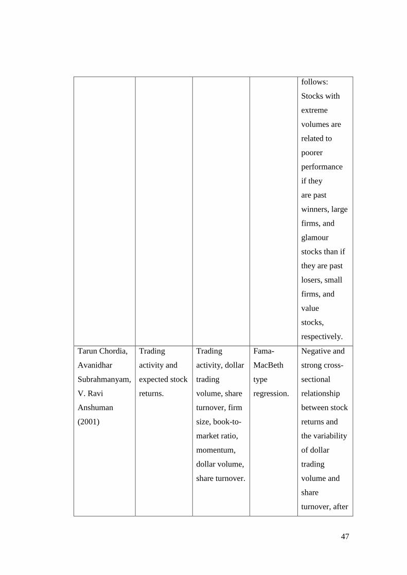
47

follows:

Stocks with

extreme

volumes are

related to

poorer

performance

if they

are past

winners, large

firms, and

glamour

stocks than if

they are past

losers, small

firms, and

value

stocks,

respectively.

Tarun Chordia,

Avanidhar

Subrahmanyam,

V. Ravi

Anshuman

(2001)

Trading

activity and

expected stock

returns.

Trading

activity, dollar

trading

volume, share

turnover, firm

size, book-to-

market ratio,

momentum,

dollar volume,

share turnover.

Fama-

MacBeth

type

regression.

Negative and

strong cross-

sectional

relationship

between stock

returns and

the variability

of dollar

trading

volume and

share

turnover, after

48

controlling for

size, book-to-

market ratio,

momentum,

and the level

of dollar

volume or

share

turnover. This

effect

survives a

number of

robustness

checks, and is

statistically

and

economically

significant.

This analysis

demonstrates

the

importance of

trading

activity-

related

variables in

the

crosssection

of expected

stock returns.

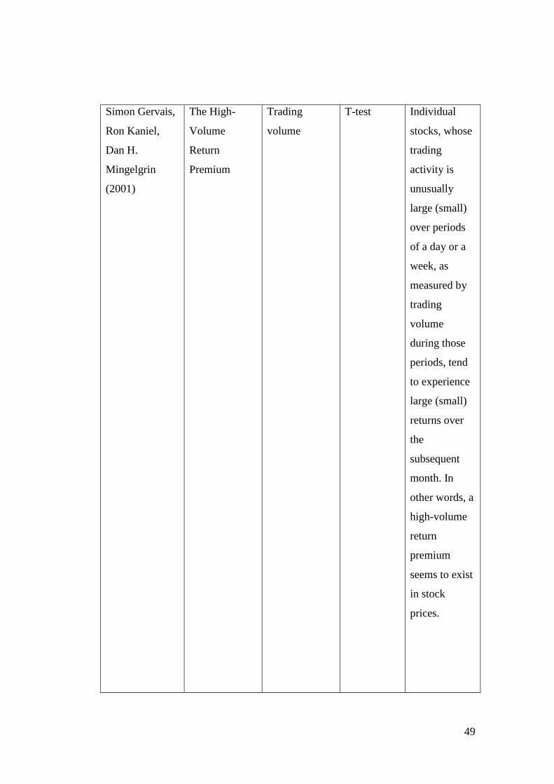
49

Simon Gervais,

Ron Kaniel,

Dan H.

Mingelgrin

(2001)

The High-

Volume

Return

Premium

Trading

volume

T-test Individual

stocks, whose

trading

activity is

unusually

large (small)

over periods

of a day or a

week, as

measured by

trading

volume

during those

periods, tend

to experience

large (small)

returns over

the

subsequent

month. In

other words, a

high-volume

return

premium

seems to exist

in stock

prices.

50

Malcolm Baker

Jeremy C. Stein

(2004)

Market

Liquidity as a

Sentiment

Indicator

Trading

Volume, Price,

Share

Turnover, Bid-

Ask Spread,

Equity

Issuance.

Multiple

regression

A model to

determine

relationship

between

liquidity

measures to

expected

return. It

found that an

unusually

liquid market

is one in

which pricing

is being

dominated by

irrational

investors, who

tend to

underreact to

the

information

embodied in

either order

flow or equity

issues. Thus

high liquidity

is a sign that

the sentiment

of these

irrational

investors is

51

positive, and

that expected

returns are

therefore

abnormally

low.

Eugene F. Fama

and Kenneth R.

French (1993)

Common Risk

Factors in The

Returns on

Stocks and

Bonds

Firm Size,

Book-to-

Market Value,

Maturity,

Default Risks.

Time-Series

Regression

Approach

Stock returns

have shared

variation due

to the stock-

market

factors, and

they are

linked to bond

returns

through

shared

variation in

the bond-

market

factors.

Generally, the

bond-market

factors

capture the

common

variation in

bond returns.

Most

important the

five factors

52

seem to

explain

average

returns on

stocks and

bonds. Firms

that have high

BE/ME (a low

stock price

relative to

book value)

tend to have

low earnings

on assets, and

the low

earnings

persist for at

least five

years before

and five years

after book-to-

market equity

is measured.

Conversely

low BE/ME (a

high stock

price relative

to book value)

is associated

with high

earnings.

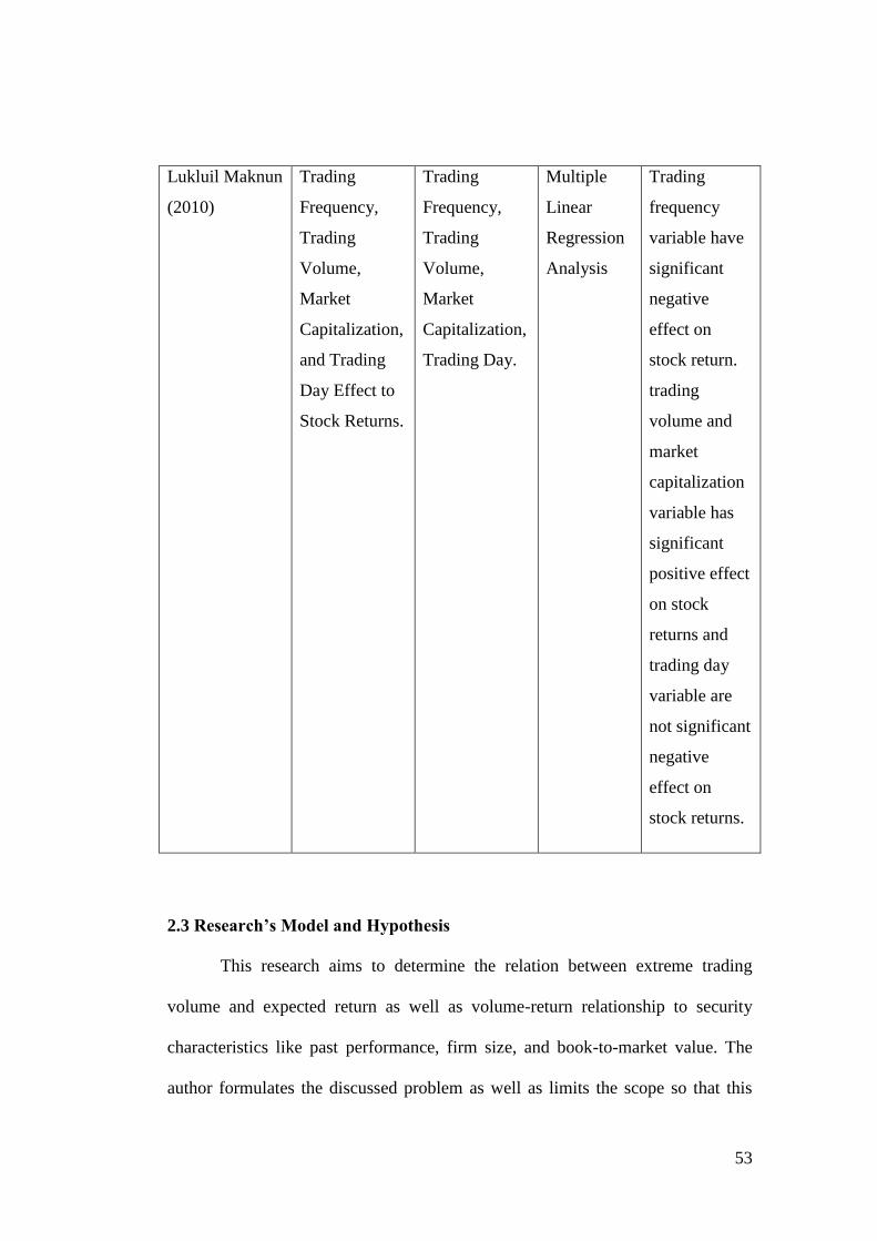
53

Lukluil Maknun

(2010)

Trading

Frequency,

Trading

Volume,

Market

Capitalization,

and Trading

Day Effect to

Stock Returns.

Trading

Frequency,

Trading

Volume,

Market

Capitalization,

Trading Day.

Multiple

Linear

Regression

Analysis

Trading

frequency

variable have

significant

negative

effect on

stock return.

trading

volume and

market

capitalization

variable has

significant

positive effect

on stock

returns and

trading day

variable are

not significant

negative

effect on

stock returns.

2.3 Research’s Model and Hypothesis

This research aims to determine the relation between extreme trading

volume and expected return as well as volume-return relationship to security

characteristics like past performance, firm size, and book-to-market value. The

author formulates the discussed problem as well as limits the scope so that this

54

discussion can be more focused. This study will also present the research model

along with appropriate analytical methods in order to achieve the purpose of the

research. After that, author will collect the necessary data and process it with the

appointed research model, analysis, and statistical methods. Conclusions of the

research will be drawn from the processes.

The data required in this study consist of the factors that influence

expected stock return of companies traded in Indonesia Stock Exchange. The

factor that affect expected stock return including liquidity which proxy by trading

volume, and securities characteristics such as past performance which proxy by

stock price, firm size which proxy by market capitalization, and security’s loading

on rational risk factors which proxy by book-to-market (BM) value.

1. Extreme Trading Volume And Expected Return

Based on Brennan et. al. (1998), Datar et. al. (1998) and Chordia et. al.

(2001) use dollar volume and share turnover as proxies for liquidity and find

negative relation between stock returns and those liquidity measures. These

foundings are consistent with Amihud and Mendelson (1986) theory called

liquidity premium hypothesis. Baker and Stein (2004) stated that liquidity is also a

sentiment indicator of irrational investors to short-sales constraint. If a large

volume of winner stocks indicate that irrational investors dominate the market, it

made trading volume is a good proxy for liquidity. Irrational investor will pushed

stock prices over its fundamental value and usually will dropped back later,

resulting in in a negative volume-return relation. Therefore, there are negative

relation between volume and returns. Lee and Swaminathan (2000) study shows

55

that past trading volume provides an important link between momentum and

strategies. Along with finding that past trading volume also can be used to predict

both magnitude and persistence of price momentum. The investor irrationality-

induced volume-return relation is referred as behavioral hypothesis.

Moreover, in the different market, when there are stocks that strongly

attracted the market, whether because its high trading or low volume, as long as it

attracts the attention of the market, there are high possibility of these stocks to

gain price appreciation, as said by Miller (1977). Consistent with this argument,

Gervais et. al. (2001) also found that there are positive relationship between

extreme trading volume and stock returns during their research at NYSE.

H1: There is a difference in expected returns between extreme high

volume and extreme low volume portfolios in Indonesia Stock Exchange

during 2008-2012 period.

2. Extreme Trading Volume and Past Performance

Past performance has been known to have an effect towards trading

volume. Deloitte & Touche’s 2001 survey of online securities also shows that the

declining in stock prices at the previous period has led to slower growth of new

online accounts and reduces trading volumes. Therefore, there might be relations

between past performance and expected return. Glaser and Weber (2005) said,

high return makes people overconfident and as a consequence, this investor trade

more subsequently. Barber and Odean (2002) analyzed a data set from a U.S

discount broker and found that high past portfolio returns induce individual

56

investors to trade more subsequently. In the other hand, similarly, Statman,

Thorley, and Vorkink (2004) find that market wide trading volume in the United

States is related to past market returns. Griffin, Nardari, and Stulz (2005) analyze

the dynamic relation market-wide trading activity and returns in 46 countries and

show that many stock markets exhibit a strong relation between trading and past

returns. Baker and Stein (2004) said that stocks that experience extreme volumes

are associated with lower expected returns for past winners than for past losers if

trading volume is a sentiment indicator.

H2: There is a difference in expected returns between extreme high

volume-winner stocks and extreme low volume-loser stocks portfolios in

Indonesia Stock Exchange during 2008-2012 period.

3. Extreme Trading Volume and Firm Size

Bamber (1986, 1987) found a negative relation between firm size and

trading volume. Based on the firm size, investor reaction to extreme trading

volume and expected return might be different. This security characteristic will be

used to see how firm size influence investor sentiment towards volume-return

relationship. Analyses on how the extreme volume-return relationship varies with

firm size also help to distinguish between the liquidity premium and the

behavioral hypotheses. Large stocks usually associated to be more liquid

compared to small stocks, therefore we expect that the extreme volume-return

relation is more obvious for small stocks than for large stocks if trading volume

proxies for liquidity.

57

H3: There is a difference in expected returns between extreme high

volume-large stocks and extreme low-small stocks portfolios in Indonesia

Stock Exchange during 2008-2012 period.

4. Extreme Trading Volume and Book-to-Market Value

Wang and Cheng (2004) said that a security’s BM is shown to be one of

the important characteristic associated with the variation in the cross section on

expected returns. Fama and French (1993, 1996) state that BM is a proxy for

security’s loadings on rational risk factors, whereas Lakonishok et. al. (1994)

argue that BM effects represent the premium for relative distress, which is caused

by investor irrationality. If BM effects caused by investor irrationality and trading

volume also proxies the sentiment of irrational investors, this research would

expect that the BM effect is associated with trading volume. In particular, low-

BM stocks that experience extremely high volumes are associated with lower

returns than those experiencing extremely low volumes.

H4: There is a difference in expected returns between extreme high

volume-glamour stocks and extreme low volume-value stocks portfolios in

Indonesia Stock Exchange during 2008-2012 period.

Some of the variables described above can be presented as following

operational and theoretical framework:

58

Figure 2. 1

Operational Framework

Data grouped into interval which include 7 weeks reference period and 1

week formation period

Portfolios sorted by volume into decile at formation period and evaluated

during evaluation period.

During 7 weeks reference period portfolios sorted by volume into quartile

and then sorted by return into quartile. The portfolios formed in formation

period based on stocks performance during reference period. The portfolios

then evaluated during evaluation period.

Portfolios sorted by volume into quartile and then sorted by firm size into

quartile and evaluated during evaluation period.

Portfolios sorted by volume into quartile and then sorted by book-to-market

value into quartile and evaluated during evaluation period.

Result and Analysis

59

Extreme Low Volume Extreme High Volume

T-Test

Extreme High Volume

Winner Stocks

Extreme Low Volume

Loser Stocks

T-Test

Extreme High Volume

Large Stocks

Extreme Low Volume

Small Stocks

T-Test

Extreme High Volume

Glamour Stocks

Extreme Low Volume

Value Stocks

T-Test

Figure 2. 2

Theoretical Framework

60

5. Research Hypothesis

Based on previous research and theoretical framework above, for the time

about the hypotheses developed as follows:

1) H1: There is a difference in expected returns between extreme high

volume and extreme low volume portfolios in Indonesia Stock Exchange

during 2008-2012 period.

2) H2: There is a difference in expected returns between extreme high

volume-winner stocks and extreme low volume-loser stocks portfolios in

Indonesia Stock Exchange during 2008-2012 period.

3) H3: There is a difference in expected returns between extreme high

volume-large stocks and extreme low volume-loser stocks portfolios in

Indonesia Stock Exchange during 2008-2012 period.

4) H4: There is a difference in expected returns between extreme high

volume-glamour stocks portfolios and extreme low volume-value stocks

portfolios in Indonesia Stock Exchange during 2008-2012 period.

61

CHAPTER III

RESEARCH METHODS

This research ought to test the defined hypotheses using determined

method. In this chapter this research will define research samples, data, data

collection method, data sources, and data analysis method.

3.1 Research Variables and Operational Variables Definition

Research variable is an attribute that as a particular variant set by this

research to be learned and drawn the conclusion from. Thus study used two types

of variables, which are input and output variables. Input variables are the trading

volume and other security characteristics which affect the expected return. The

output is the return itself.

The variables used in this study were based on the literature review.

Research variables used at tis research are as follows:

3.1.1 Return

Ang (1997) definition about return is the rate of profit that gained by the

investor from its investment. Investor motivated to invest their money with

expectation to gain a proper return. Without guarantee to gain return, investor will

reluctant to invest. Ang also said that return has been an investor prime motive

despite the type of the investment, whether it’s a long term or short term

investment.

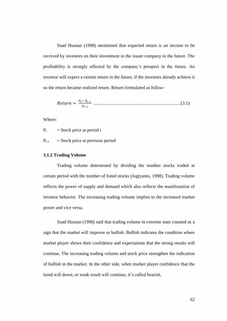
62

Suad Husnan (1998) mentioned that expected return is an income to be

received by investors on their investment in the issuer company in the future. The

profitability is strongly affected by the company’s prospect in the future. An

investor will expect a certain return in the future, if the investors already achieve it

so the return became realized return. Return formulated as follow:

............................................................................(3.1)

Where:

Pt = Stock price at period t

Pt-1 = Stock price at previous period

3.1.2 Trading Volume

Trading volume determined by dividing the number stocks traded at

certain period with the number of listed stocks (Jogiyanto, 1998). Trading volume

reflects the power of supply and demand which also reflects the manifestation of

investor behavior. The increasing trading volume implies to the increased market

power and vice versa.

Suad Husnan (1998) said that trading volume in extreme state counted as a

sign that the market will improve or bullish. Bullish indicates the condition where

market player shows their confidence and expectations that the strong results will

continue. The increasing trading volume and stock price strengthen the indication

of bullish in the market. In the other side, when market player confidence that the

trend will down, or weak result will continue, it’s called bearish.

63

This research will sorted all stocks in each formation period to decile

based on trading volumes. A stock is classified as extreme high volume stock if its

position is in the top 10% or decile 1. On the other hand, a stock is classified as

extreme low volume stock if its position is on the bottom 10% or decile 10.

3.1.3 Past Performance

Wang and Cheng (2004) defined past performance as the achievement of

one stocks, whether is gain or lose, during periods prior to current time or

formation period (in portfolio forming case). Past performance often associated

with investor confidence towards certain stocks. Some theories argue that high

returns make investors overconfident and as a consequence these investors trade

more subsequently.

This research will sorted all stocks in two steps. After sorted to quartile

based on the trading volume, it will sorted again based on the returns. A stock is

classified as winner stock if its returns are in the top 25% or quartile 1 during 7

weeks of reference formation prior to each formation period and a stock is

classified as loser stock if its returns are in the bottom 25% or quartile 4 during 7

week reference period prior to each formation period.

3.1.4 Firm Size

Horne and Wachowichz (1997) describe firm size as total assets of a

company and can be seen in the left side of the balance sheet. This statement goes

along with Bala and Goyal (2000) statement who also said that mathematically,

firm size can be measured by its market capitalization. Size difference reflects

64

companies’ capability to compete in the market. Market capitalization can be

measured by formula as follow:

Market Capitalization = Stock price x Outstanding stocks ..................(3.2)

This research will sorted all stocks in two steps. After sorted to quartile

based on the trading volume, it will sorted again based on the market

capitalization at the end of the year preceding the formation period. A stock is

classified as large stock if its market capitalization is among the top 25% or

quartile 1. A stock is classified as small stocks if its market capitalization is

among the bottom 25% or quartile 4.

3.1.5 Book-to-Market Value

Book to market value is stock's book value divided by its market value.

Book value is calculated from the company's balance sheet, while market value is

based on the price of its stock. A ratio above 1 indicates a potentially undervalued

stock (value stocks), while a ratio below 1 indicates a potentially overvalued stock

(glamour stocks). Technology companies and other companies in industries which

do not have a lot of physical assets tend to have low book to market ratios. Below

is the formula for Book-to-Market ratio:

Book-to-market ratio =

...................................(3.3)

This research will sorted all stocks in two steps. After sorted to quartile

based on the trading volume, it will sorted again based on the B/M value. BM

value is a ratio of the book value of the company for the fiscal year prior to the

65

formation period to the market value at the end of December prior to the

formation to the formation period. A stock is classified as glamour stock if its BM

values are among the top 25% or quartile 1 and classified as value stocks if its BM

values are among the bottom 25% or quartile 4.

66

Table 3. 1

Operational Definition

Variable Definition Formula Scale

Return The rate of

profit that

gained by the

investor from

its investment.

In percentage

(%)

Trading

Volume

The number of

stock traded at

the certain

period.

In numeric

number (IDR)

Past

Performance

The

achievement of

one stocks,

whether is gain

or lose, during

periods prior to

current time or

formation

period.

Return of t-1 In percentage

(%)

Firm Size Total assets of a

company.

Stock price x Outstanding

stocks

In numeric

(IDR)

Book-to-Market

Value (BM)

Stock's book

value divided

by its market

value

In percentage

(%)

67

3.2 Population and Research Samples

Population used in this research is companies listed at Indonesia Stock

Exchange from 2008 to 2012 period. Sampling method used in this research are

non-random sampling and purposive sampling. Purposive sampling is used to

determine sample selection, which means non-probability sample which custom

designed to exact criteria depends on the research. Criteria used are as follows:

a. Stocks traded at Indonesia Stock Exchange at least 6 months prior to the

formation period or 1 January 2008.

b. Stocks that are banks, investment trust, real estate, and investment

companies are excluded.

c. The firm must have available information on trading volume and relevant

accounting data during research period.

d. Samples must be actively traded during research period.

After purposive sampling has done, this research have 80 stocks as

samples which meet the requirements above. The list of the samples can be found

at appendix.

3.3 Data Type and Source

Type of data used in this research is secondary data, which is data that not

obtained by researcher directly. Secondary data is a data compiled by bank data

from institution or organization and published to public and data user. As said by

Sekaran (2000), secondary data are company resources or archive, government

publication, and industry analysis offered by media such as website, paper release,

68

internet, and other publication. Data used in this research are secondary data as

follows:

a. Trading volume for each sample during research period

b. Historical data for each sample during research period

c. Size/market capitalization for each sample during research period

d. Book-to-market value for each sample during research period

In this research, secondary data obtained from books, journal, thesis,

articles, and websites related to the topics which have been selected such as those

reports which published in range 2008-2012 of range.

3.4 Data Collection Method

Data in this research are collected by following methods:

1. Documentation

Documentation performed by data collection from bank data like

Indonesia Stock Exchange Corner or by downloading data objects via

websites. Websites used as source of this research are as follows:

a. www.idx.com

b. finance.yahoo.com

2. Sampling Method

Samples picked non-randomly. Sampling method used in this research is

purposive sampling. It means samples are picked and designed to fulfill

several requirements to be count as proper for the research. The number of

69

samples is not specifically designated. It may be as many as possible as

long those samples meet the requirements.

3. Literature Study

Literature study used to collect data which couldn’t be obtained from

financial report or historical data like theories, definitions, previous

research, etc. The data was obtained from books, journals, thesis,

magazines, websites, etc.

3.5 Data Analysis

This research will use quantitative analytical methods. Quantitative

analytical methods used in this research such as mathematics and statistical

models. Mathematics models to determine the variables and statistical models to

determine the characteristics of the data.

3.5.1 Stock Formation

Stock formation period in this research is one week. Portfolios are formed

using a reference return portfolio approach similar to that of Gervais et. al. (2001).

The weekly sample is constructed as follows. The time interval between January

2008 and December 2012 is divided into 29 non-overlapping intervals. Each

trading interval consists of a 7-week reference period and a 1-week formation

period with 1 week lag between reference period to formation period. The lag is

allowed to avoid possible bid-ask spread and lead-lag effects.

In this research, due to the time constraints there will be only 26 intervals

mainly calculated. It is noted that the extreme volume as defined previously is an

70

indirect measure of liquidity same as share turnover, when the firm’s total share

outstanding remains unchanged over the reference and formation periods.

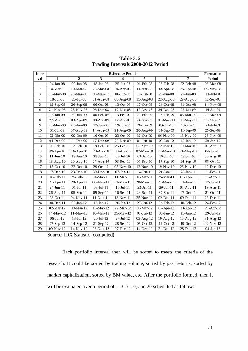
71

Table 3. 2

Trading Intervals 2008-2012 Period

Inter

val

Reference Period Formation

Period 1 2 3 4 5 6 7

1 04-Jan-08 09-Jan-08 18-Jan-08 25-Jan-08 01-Feb-08 06-Feb-08 22-Feb-08 06-Mar-08

2 14-Mar-08 19-Mar-08 28-Mar-08 04-Apr-08 11-Apr-08 18-Apr-08 25-Apr-08 09-May-08

3 16-May-08 23-May-08 30-May-08 06-Jun-08 13-Jun-08 20-Jun-08 27-Jun-08 11-Jul-08

4 18-Jul-08 25-Jul-08 01-Aug-08 08-Aug-08 15-Aug-08 22-Aug-08 29-Aug-08 12-Sep-08

5 19-Sep-08 26-Sep-08 06-Oct-08 13-Oct-08 17-Oct-08 24-Oct-08 31-Oct-08 14-Nov-08

6 21-Nov-08 28-Nov-08 05-Dec-08 12-Dec-08 19-Dec-08 26-Dec-08 05-Jan-09 16-Jan-09

7 23-Jan-09 30-Jan-09 06-Feb-09 13-Feb-09 20-Feb-09 27-Feb-09 06-Mar-09 20-Mar-09

8 27-Mar-09 03-Apr-09 08-Apr-09 17-Apr-09 24-Apr-09 01-May-09 08-May-09 22-May-09

9 29-May-09 05-Jun-09 12-Jun-09 19-Jun-09 26-Jun-09 03-Jul-09 10-Jul-09 24-Jul-09

10 31-Jul-09 07-Aug-09 14-Aug-09 21-Aug-09 28-Aug-09 04-Sep-09 11-Sep-09 25-Sep-09

11 02-Okt-09 09-Oct-09 16-Oct-09 23-Oct-09 30-Oct-09 06-Nov-09 13-Nov-09 26-Nov-09

12 04-Dec-09 11-Dec-09 17-Dec-09 23-Dec-09 04-Jan-10 08-Jan-10 15-Jan-10 29-Jan-10

13 05-Feb-10 12-Feb-10 19-Feb-10 25-Feb-10 05-Mar-10 12-Mar-10 19-Mar-10 01-Apr-10

14 09-Apr-10 16-Apr-10 23-Apr-10 30-Apr-10 07-May-10 14-May-10 21-May-10 04-Jun-10

15 11-Jun-10 18-Jun-10 25-Jun-10 02-Jul-10 09-Jul-10 16-Jul-10 23-Jul-10 06-Aug-10

16 13-Aug-10 20-Aug-10 27-Aug-10 03-Sep-10 07-Sep-10 17-Sep-10 24-Sep-10 08-Oct-10

17 15-Oct-10 22-Oct-10 29-Oct-10 05-Nov-10 12-Nov-10 19-Nov-10 26-Nov-10 10-Dec-10

18 17-Dec-10 23-Dec-10 30-Dec-10 07-Jan-11 14-Jan-11 21-Jan-11 28-Jan-11 11-Feb-11

19 18-Feb-11 25-Feb-11 04-Mar-11 11-Mar-11 18-Mar-11 25-Mar-11 01-Apr-11 15-Apr-11

20 21-Apr-11 29-Apr-11 06-May-11 13-May-11 20-May-11 27-May-11 01-Jun-11 17-Jun-11

21 24-Jun-11 01-Jul-11 08-Jul-11 15-Jul-11 22-Jul-11 29-Jul-11 05-Aug-11 19-Aug-11

22 26-Aug-11 05-Sep-11 09-Sep-11 16-Sep-11 23-Sep-11 30-Sep-11 07-Oct-11 21-Oct-11

23 28-Oct-11 04-Nov-11 11-Nov-11 18-Nov-11 25-Nov-11 02-Dec-11 09-Dec-11 23-Dec-11

24 30-Dec-11 06-Jan-12 13-Jan-12 20-Jan-12 27-Jan-12 03-Feb-12 10-Feb-12 24-Feb-12

25 02-Mar-12 09-Mar-12 16-Mar-12 22-Mar-12 30-Mar-12 05-Apr-12 13-Apr-12 27-Apr-12

26 04-May-12 11-May-12 16-May-12 25-May-12 01-Jun-12 08-Jun-12 15-Jun-12 29-Jun-12

27 06-Jul-12 13-Jul-12 20-Jul-12 27-Jul-12 03-Aug-12 10-Aug-12 16-Aug-12 31-Aug-12

28 07-Sep-12 14-Sep-12 21-Sep-12 28-Sep-12 05-Oct-12 12-Oct-12 19-Oct-12 02-Nov-12

29 09-Nov-12 14-Nov-12 23-Nov-12 07-Dec-12 14-Dec-12 21-Dec-12 28-Dec-12 04-Jan-13

Source: IDX Statistic (computed)

Each portfolio interval then will be sorted to meets the criteria of the

research. It could be sorted by trading volume, sorted by past returns, sorted by

market capitalization, sorted by BM value, etc. After the portfolio formed, then it

will be evaluated over a period of 1, 3, 5, 10, and 20 scheduled as follow:

72

Figure 2. 3

Evaluation Period

Interval Formation Period Evaluation Period

1 3 5 10 20

1 06-Mar-08 19-Mar-08 04-Apr-08 18-Apr-08 23-May-08 01-Ags-08

2 09-May-08 23-May-08 06-Jun-08 20-Jun-08 25-Jul-08 06-Okt-08

3 11-Jul-08 25-Jul-08 08-Aug-08 20-Aug-08 26-Sep-08 05-Dec-08

4 12-Sep-08 26-Sep-08 13-Oct-08 24-Oct-08 28-Nov-08 06-Feb-09

5 14-Nov-08 28-Nov-08 12-Dec-08 26-Dec-08 30-Jan-09 08-Apr-09

6 16-Jan-09 30-Jan-09 13-Feb-09 27-Feb-09 03-Apr-09 12-Jun-09

7 20-Mar-09 03-Apr-09 17-Apr-09 01-May-09 05-Jun-09 14-Aug-09

8 22-May-09 05-Jun-09 19-Jun-09 03-Jul-09 07-Aug-09 16-Oct-09

9 24-Jul-09 07-Aug-09 21-Aug-09 04-Sep-09 09-Oct-09 17-Dec-09

10 25-Sep-09 09-Oct-09 23-Oct-09 06-Nov-09 11-Dec-09 19-Feb-10

11 26-Nov-09 11-Dec-09 23-Dec-09 08-Jan-10 12-Feb-10 23-Apr-10

12 29-Jan-10 12-Feb-10 25-Feb-10 12-Mar-10 16-Apr-10 25-Jun-10

13 01-Apr-10 16-Apr-10 30-Apr-10 14-May-10 18-Jun-10 27-Aug-10

14 04-Jun-10 18-Jun-10 02-Jul-10 16-Jul-10 20-Aug-10 29-Oct-10

15 06-Aug-10 20-Aug-10 03-Sep-10 17-Sep-10 22-Oct-10 30-Dec-10

16 08-Oct-10 22-0ct-10 05-Nov-10 19-Nov-10 23-Dec-10 04-Mar-11

17 10-Dec-10 23-Dec-10 07-Jan-11 21-Jan-11 25-Feb-11 06-May-11

18 11-Feb-11 25-Feb-11 11-Mar-11 25-Mar-11 29-Apr-11 08-Jul-11

19 15-Apr-11 29-Apr-11 13-May-11 27-May-11 01-Jul-11 09-Sep-11

20 17-Jun-11 01-Jul-11 15-Jul-11 29-Jul-11 05-Sep-11 11-Nov-11

21 19-Aug-11 05-Sep-11 16-Sep-11 30-Sep-11 04-Nov-11 13-Jan-12

22 21-Oct-11 04-Nov-11 18-Nov-11 02-Dec-11 06-Jan-12 16-Mar-12

23 23-Dec-11 06-Jan-12 20-Jan-12 03-Feb-12 09-Mar-12 16-May-12

24 24-Feb-12 09-Mar-12 22-Mar-12 05-Apr-12 11-May-12 20-Jul-12

25 27-Apr-12 11-May-12 25-May-12 08-Jun-12 13-Jul-12 21-Sep-12

26 29-Jun-12 13-Jul-12 27-Jul-12 10-Aug-12 14-Sep-12 23-Nov-12

Source: IDX Statistic (computed)

3.5.2 T-test

T-test used in this research is paired T-test. The purpose of this test is to

determine the difference of the samples. Paired sample is a sample with the same

subject but under different treatments or measurements. Test performed by T-test

and compared the result with T-table. T-test performed in this research used to

73

compare returns of each evaluation period with 2-tails, 25 degree of freedom, and

95% confidence level. Thus the following requirements are as follows:

If p value > 0.05, then it means average return of both samples is identic or

there is no difference at all.

If p value < 0.05, then it means average return of both samples is not

identic or they are higher or lower.

There will be 4 part of the T-Test which will be performed on each

hypotheses testing. Generally, there will be T-test to differentiate returns for high

volume portfolios at formation period and evaluation period, T-test to differentiate

returns for low volume portfolios at formation period and evaluation period, T-test

to differentiate returns between high and low volume portfolios at formation

period and evaluation period, and the last one is T-test to differentiate returns of

high and low volume portfolios at each evaluation period.

3.5.3 Hypothesis Testing

1. First Hypothesis testing, “There is a difference in expected returns between

extreme high volume and extreme low volume portfolios in Indonesia Stock

Exchange during 2008-2012 period”

The reference portfolios is the equal weight average of the Indonesia

composite index (IHSG), which is a proxy for the market portfolio. This

approach has two advantages: first, weights for each trading interval are

implicitly adjusted according to the number of stocks experiencing high and

low volumes during the interval; and second, since each long position is offset

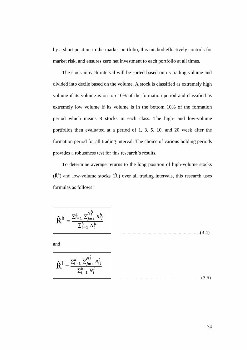
74

by a short position in the market portfolio, this method effectively controls for

market risk, and ensures zero net investment to each portfolio at all times.

The stock in each interval will be sorted based on its trading volume and

divided into decile based on the volume. A stock is classified as extremely high

volume if its volume is on top 10% of the formation period and classified as

extremely low volume if its volume is in the bottom 10% of the formation

period which means 8 stocks in each class. The high- and low-volume

portfolios then evaluated at a period of 1, 3, 5, 10, and 20 week after the

formation period for all trading interval. The choice of various holding periods

provides a robustness test for this research’s results.

To determine average returns to the long position of high-volume stocks

(Ȓh) and low-volume stocks (Ȓ

l) over all trading intervals, this research uses

formulas as follows:

...............................................................(3.4)

and

................................................................(3.5)

Ȓh = ∑ ∑

∑

Ȓl = ∑ ∑

∑

75

Whereas:

Ȓh = return to high-volume stock

Ȓl = return to low-volume stock

i = trading interval

= number of high-volume stock

= number of low-volume stock

k = number of trading intervals

After all average returns in each trading interval calculated, T-test will be

performed to determine the difference between extreme high volume and

extreme low volume portfolios through the evaluation periods. H1 will be

accepted if p value is < 0.050.

2. Second Hypothesis testing, “There is a difference in expected returns between

extreme high volume-winner stocks and extreme low volume-loser stocks

portfolios in Indonesia Stock Exchange during 2008-2012 period”

Baker and Stein (2004) said that stocks that experience extreme volumes

are associated with lower expected returns for past winners than for past losers

if trading volume acted as a sentiment indicator. The liquidity premium

hypothesis does not appear to suggest a priori relation between liquidity

premiums and past stock performance. Thus, evidence on the variation of

volume–return relation with past stock performance is useful to distinguish

between the behavioral and the liquidity premium hypotheses.

76

To proceed, this research compute average returns to portfolios formed by

interacting between extreme volumes and past stock performance. In each

reference period in one trading interval, stocks are first classified into high and

low volume by its trading volume. Different from the volume-return testing,

this time the stock divided into quartile based on its volume. A stock is

classified as extremely high-volume if its volume is in the top 25% of the

reference period and classified as extremely low-volume if its volume is in the

bottom 25% of the reference period. So the extreme high and extreme low class

is each consisted of 20 stocks. Then both class sorted again by its return and

each divided into quartile. A stock is classified as winner if its return is among

the top 25% of the high-volume class and classified as loser if its return is

among the bottom 25% of the low-volume class. So there are 5 stocks labeled

as high volume-winner and 5 stocks labeled low volume-loser in a reference

period. A final portfolio will formed at the formation period at the end of

reference periods which consist of stocks which remain at the top 25% and

bottom 25% during prior 7 weeks reference periods.

The high volume-winner stocks and low volume-loser stocks portfolios

formed at formation period then evaluated over a period of 1, 3, 5, 10, and 20

weeks evaluation period to determine the performance. To determine average

returns to the long position of extreme high-volume stocks (Ȓh) and extreme

low-volume stocks (Ȓl) over all trading intervals will be the same with the

previous testing and will be used for the rest of the testing. After all average

returns in each trading interval calculated, T-test will be performed to

77

determine the difference between extreme high volume-winner stocks and

extreme low volume-loser stocks portfolios through the evaluation periods. H2

will be accepted if - p value is < 0.050.

3. Third Hypothesis Testing, “There is a difference in expected returns between

extreme high volume-large stocks and extreme low volume-loser stocks

portfolios in Indonesia Stock Exchange during 2008-2012 period”

Analysis on how extreme volume and return varies with firm size also

helps distinguish between the liquidity premium and the behavioral hypotheses.

Usually, large stocks are in general more liquid than small stocks. Therefore,

this research expect that the extreme volume–return relation is more

pronounced for small stocks than for large stocks if trading volume proxies for

liquidity. A different finding tends to tilt our inference towards the alternative

hypothesis—the behavioral hypothesis.

To examine this issue, we form portfolios by interacting between firm size

and extreme volumes. Using the similar technique discussed previously, in

each formation period, first sort all eligible stocks into high and low volume

groups based on the volume. A stock is classified as extreme high volume if its

volume is in the top 25% and classified as extreme low volume if its volume is

in the bottom 25% so each class has 20 stocks. In each size sorted group,

stocks are further split into the large or small stocks by sorting it based on its

market capitalization as the measurement of size. A stock is classified as large

stock if its size is among the top 25% and classified as small stock if its size is

78

among the bottom 25% and therefore, there will be 5 stocks labeled as extreme

high volume-large stocks and extreme low volume-small stocks in each group.

The extreme high volume-large stocks and extreme low volume-small

stocks portfolios formed at formation period then evaluated over a period of 1,

3, 5, 10, and 20 weeks evaluation period to determine the performance. After

all average returns in each trading interval calculated, T-test will be performed

to determine the difference between extreme high volume-large stocks and

extreme low volume-small stocks portfolios through the evaluation periods. H3

will be accepted if p value is < 0.050.

4. Fourth Hypothesis Testing, “There is a difference in expected returns between

extreme high volume-glamour stocks portfolios and extreme low volume-value

stocks portfolios in Indonesia Stock Exchange during 2008-2012 period.”

A security’s BM is shown to be one of the important firm characteristics

associated with the variation in the cross section of expected returns. Fama and

French (1993, 1996) contend that BM is a proxy for the security’s loadings on

rational risk factors, whereas Lakonishok et. al. (1994) argue that the BM

effect represents the premium for relative distress, which is caused by investor

irrationality. If BM effect is caused by investor irrationality and trading volume

also proxies the sentiment of irrational investors, there will be expectation that

the BM effect is associated with trading volume. In particular, low-BM stocks

that experience extremely high volumes are associated with lower returns than

those experiencing extremely low volumes.

79

To examine this possibility, this research use the same sorting technique as

before, and first sort all eligible stocks into high and low volume groups based

on the volume. A stock is classified as extreme high volume stock if its volume

is in the top 25% and classified as extreme low volume stock if its volume is in

the bottom 25% so each class has 20 stocks. In each size sorted group, stocks

are further split into the glamour or value stocks by sorting it based on its BM

value. A stock is classified as glamour stock if its BM value is among the

bottom 25% of the high volume group and classified as value stock if its size is

among the top 25% of the low volume group. Therefore, there will be 5 stocks

labeled as extreme high volume-glamour stocks and extreme low volume-value

stocks in each group.

The extreme high volume-glamour stocks and extreme low volume-value

stocks portfolios formed at formation period then evaluated over a period of 1,

3, 5, 10, and 20 weeks evaluation period to determine the performance. After

all average returns in each trading interval calculated, T-test will be performed

to determine the difference between extreme high volume-glamour stocks and

extreme low volume-value stocks portfolios through the evaluation periods. H4

will be accepted if p value is < 0.050.