extreme scale unstructured adaptive cfd: from multiphase
TRANSCRIPT
ANL/ALCF/ESP-17/8
Extreme Scale Unstructured Adaptive CFD: FromMultiphase Flow to Aerodynamic Flow Control
Technical Report for the ALCF Theta Early Science Program
Argonne Leadership Computing Facility
ALCF Early Science Program (ESP) Technical Report
ESP Technical Reports describe the code development, porting, and optimization done in preparing an ESP project’s
application code(s) for the next generation ALCF computer system. This report is for a project in the Theta ESP, preparing
for the ALCF Theta computer system.
About Argonne National LaboratoryArgonne is a U.S. Department of Energy laboratory managed by UChicago Argonne, LLCunder contract DE-AC02-06CH11357. The Laboratory’s main facility is outside Chicago, at9700 South Cass Avenue, Argonne, Illinois 60439. For information about Argonneand its pioneering science and technology programs, see www.anl.gov.
DOCUMENT AVAILABILITY
Online Access: U.S. Department of Energy (DOE) reports produced after 1991 and agrowing number of pre-1991 documents are available free at OSTI.GOV(http://www.osti.gov/), a service of the U.S. Dept. of Energy’s Office of Scientific andTechnical Information
Reports not in digital format may be purchased by the public from theNational Technical Information Service (NTIS):
U.S. Department of CommerceNational Technical Information Service5301 Shawnee RdAlexandria, VA 22312www.ntis.govPhone: (800) 553-NTIS (6847) or (703) 605-6000Fax: (703) 605-6900Email: [email protected]
Reports not in digital format are available to DOE and DOE contractors from theOffice of Scientific and Technical Information (OSTI):
U.S. Department of EnergyOffice of Scientific and Technical InformationP.O. Box 62Oak Ridge, TN 37831-0062www.osti.govPhone: (865) 576-8401Fax: (865) 576-5728Email: [email protected]
DisclaimerThis report was prepared as an account of work sponsored by an agency of the United States Government. Neither the United StatesGovernment nor any agency thereof, nor UChicago Argonne, LLC, nor any of their employees or officers, makes any warranty, express orimplied, or assumes any legal liability or responsibility for the accuracy, completeness, or usefulness of any information, apparatus,product, or process disclosed, or represents that its use would not infringe privately owned rights. Reference herein to any specificcommercial product, process, or service by trade name, trademark, manufacturer, or otherwise, does not necessarily constitute or imply itsendorsement, recommendation, or favoring by the United States Government or any agency thereof. The views and opinions of documentauthors expressed herein do not necessarily state or reflect those of the United States Government or any agency thereof, ArgonneNational Laboratory, or UChicago Argonne, LLC.
ANL/ALCF/ESP-17/8
Extreme Scale Unstructured Adaptive CFD: From Multi-phase Flow to Aerodynamic Flow Control
Technical Report for the ALCF Theta Early Science Program
edited byTimothy J. Williams and Ramesh Balakrishnan
Argonne Leadership Computing Facility
prepared byKenneth E. Jansen, Michel Rasquin, John A. Evans, Jed Brown, Chris Carothers, Mark S. Shephard,Onkar Sahni, Cameron W. Smith, Jun Fang, and Igor Bolotnov
September 2017
This work was supported in part by the Office of Science, U.S. Department of Energy, under Contract DE-AC02-06CH11357.

Extreme Scale Unstructured Adaptive CFD: From
Multiphase Flow to Aerodynamic Flow Control
Kenneth E. Jansen∗1, Michel Rasquin1, John A. Evans1, Jed Brown1, Chris Carothers2,Mark S. Shephard2, Onkar Sahni2, Cameron W. Smith2, Jun Fang3, and Igor Bolotnov4
1 University of Colorado Boulder, Boulder, Colorado 80309, USA2 Rensselaer Polytechnic Institute, Troy, New York 12180, USA3 Argonne National Laboratory, Lemont, Illinois 60439, USA
4 North Carolina State University, Raleigh, North Carolina 27695, USA
1 Introduction
Understanding the flow of fluid, either liquid or gas, through and around solid bodies has chal-lenged man since the dawn of scientific inquiry. Many of the great minds of science and mathhave progressively built up a hierarchy of fluid models. This report is concerned with the compu-tational modeling of turbulent flow around aerodynamic bodies such as planes and wind turbines.In this case, viscous effects near the solid bodies create very thin boundary layers that yield highlyanisotropic (gradients normal to the surface may be 106 times larger than gradients along the sur-face) solutions to the governing non-linear partial differential equations (PDE); the Navier-Stokesequations. Furthermore, turbulent flows develop extremely broad ranges of length and time scales.This disparity motivates the use of discretization methods capable of employing adaptivity and im-plicit time integration. The combination of these features (non-linear, anisotropy, adaptivity, andimplicit) dramatically raise the complexity of the discretization, posing large challenges to efficientscalable parallel implementation. However, through careful design, the more complex algorithmscan provide great reductions in computational cost relative to simpler methods (e.g., Cartesian gridswith explicit time integration) that are easier to mate efficiently to hardware. In this report, we notonly describe our approach but we also address the fact that while complex algorithms may neverbe as efficient flop-for-flop as simple methods, in the important measure of science-per-core-hour,they can still win big by making complex features like adaptivity and implicit methods as efficientand scalable as possible.
2 Science Summary
In this section we discuss the science impact of applying our open source, massively parallel (e.g.,> 3M processes [24, 33] Fig. 1) computational fluid dynamics analysis package, PHASTA, to theapplications of active flow control for external aerodynamics.
The goal of aerodynamics is to improve the vehicle performance. Synthetic jet actuators for activeflow control [3, 11] have been shown to produce large scale flow changes (e.g., re-attachment ofseparated flow or virtual aerodynamic shaping of lifting surfaces) from micro-scale input (e.g., a
1
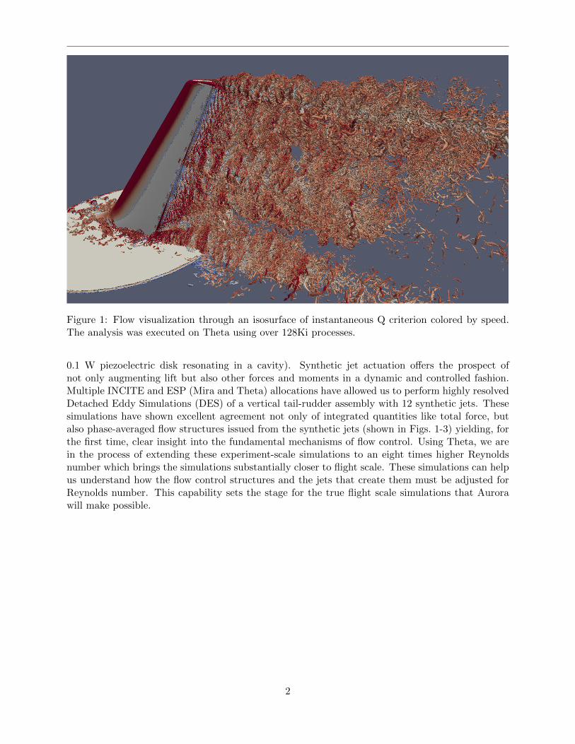
Figure 1: Flow visualization through an isosurface of instantaneous Q criterion colored by speed.The analysis was executed on Theta using over 128Ki processes.
0.1 W piezoelectric disk resonating in a cavity). Synthetic jet actuation offers the prospect ofnot only augmenting lift but also other forces and moments in a dynamic and controlled fashion.Multiple INCITE and ESP (Mira and Theta) allocations have allowed us to perform highly resolvedDetached Eddy Simulations (DES) of a vertical tail-rudder assembly with 12 synthetic jets. Thesesimulations have shown excellent agreement not only of integrated quantities like total force, butalso phase-averaged flow structures issued from the synthetic jets (shown in Figs. 1-3) yielding, forthe first time, clear insight into the fundamental mechanisms of flow control. Using Theta, we arein the process of extending these experiment-scale simulations to an eight times higher Reynoldsnumber which brings the simulations substantially closer to flight scale. These simulations can helpus understand how the flow control structures and the jets that create them must be adjusted forReynolds number. This capability sets the stage for the true flight scale simulations that Aurorawill make possible.
2

0 50 100 150 200 250 300 350 400
Jet Cycles
0.7
0.725
0.75
0.775
0.8
0.825
0.85
0.875
0.9C
YExp - 12 jets
Exp - Jet 5
Exp - BaselineA1 Baseline
A1 Jet 5
A1 12 Jets
A2 Baseline
A2 Jet 5
A2 12 Jets
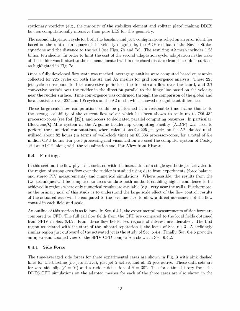
Figure 3: Time history of the CFD side force coefficient, CY , versus the jet actuation cycles com-pared with the time-averaged experimental measurements.
(a) CFD - First adapted mesh. (b) CFD - Second adapted mesh. (c) Experiments.
Figure 2: Phase-averaged isosurface of velocity (color) and vorticity (grey) revealing coherent struc-tures in the wake of a synthetic jet located at the junction between the stabilizer and the deflectedrudder of a vertical tail. Comparison between CFD predictions on two successive adapted meshesand experimental results (c).
The energy impact of such a predictive capability can best be related to its potential to reducethe size of the vertical tail and rudder, and thus reduce their significant drag contribution in thecruise condition. A recent study at Boeing estimated that a 777-class airplane could reduce its fuelconsumption by 0.75-1.0% on a 3000 Nautical mile trip if its vertical tail size could be reduced by25%. Our joint experimental/computational studies suggest that active flow control can achievethis size reduction at experiment scale. Commercial airlines consume over 20 billion (B) gallons ofjet fuel per year. Even a fairly conservative estimate of 0.5% fuel usage reduction would result in a$0.3B per year savings. For this reason, Boeing has sponsored a joint experimental-computationalstudy at Rensselaer Polytechnic Institute (Experiment and Controls) and University of Colorado(Computational). This availability of support, industrial engagement, and validation data providesstrong additional motivation for this problem. To date, we have already compared our PHASTAsimulations to experiments on the 1st, 2nd and 3rd generations of experimental facilities.
3

3 Codes, Methods and Algorithms
A mature finite-element flow solver (PHASTA) [55, 56] is paired with anisotropic adaptive meshingprocedures [15, 16, 17, 18, 42] (which we have developed within the SciDAC ITAPS and nowFASTMath project) to provide a powerful tool for attacking fluid flow problems where boundaryand shear layers develop highly anisotropic solutions that can only be located and resolved byapplying adaptive methods [9, 8]. These flow problems can involve complicated geometries such asthe human arterial system and complex physics such as fluid turbulence [14, 21, 47, 48, 49, 50] andmultiphase interactions [28, 29, 35, 5, 10, 53]. The resulting discretizations are so large that only ahighly scalable, anisotropic, adaptive flow solver capable of using massively parallel (petascale andcoming exascale) systems can yield insightful solutions in a relevant time frame.
PHASTA is a parallel, hierarchic (2nd to 5th order accurate), adaptive, stabilized (finite-element [6]),transient analysis solver for compressible or incompressible flows. It solves PDE’s typical of physi-cal problems in fluid mechanics, electromagnetics, biomechanics, etc. PHASTA and its predecessorENSA were the first massively parallel unstructured grid LES/DNS codes [19, 20, 23] and have beenapplied to flows ranging from validation benchmarks to complex cases.
The equation formation work is dominated by the computation of integrals appearing in the weakform using quadrature which, after implicit time integration [22], yields a system of non-linearalgebraic equations that are linearized and solved using either native iterative procedures [37], orPETSc [4]. Equation formation work can be tuned to specific architectures by varying the numberof elements in a block; which we will later refer to as block size. Computational load (on anyprocess) during the equation formation stage depends on the number elements assigned to the theprocess, whereas in the system solution stage the load depends on the number of vertices.
PHASTA has two forms of I/O; one file per MPI process, and MPI-IO [26]. The latter supportsreading (writing) the data of multiple processes to (from) a single file. This aggregation-basedapproach using MPI-IO has proven scalable to > 3M processes on Mira and 256Ki on Theta.PHASTA has been coded for pure MPI and MPI+X where X is currently OpenMP. While MPI+Xhas been shown to scale at better than 75% efficiency on a variety of architectures, on Mira andTheta, pure MPI has scaled at > 90% efficiency (Figs. 4, 5).
The PUMI, parallel unstructured mesh infrastructure, adaptive meshing tools have already beenported over to Mira and Theta and allowed the generation and the partitioning of a 92 billion elementmesh which was then used as a scaling benchmark of our flow solver PHASTA to> 3M processes [33].Unstructured parallel mesh adaptation procedures based on local modification operators can beused to adaptively construct the meshes required for the target applications. At PUMI’s core isan array based mesh representation component that provides efficient mechanisms to query andmodify the mesh while maintaining a small memory footprint [16, 18]. Parallel mesh operations,such as the definition of the partition graph, the migration of elements, and synchronization ofoff-process boundary data, is provided by the APF component. These parallel mesh operationsprovide the supporting functionality to implement mesh adaptation and fast dynamic load balancingcomponents, MeshAdapt [2, 30] and ParMA [40, 57], respectively.
ParMA APIs are used to (1) predictively balance mesh elements during mesh adaptation to avoidmemory exhaustion, and after adaptation operations are completed, (2) ensure that the applica-tions mesh entity balance requirements are met. For a PHASTA analysis, ParMA first targets thereduction of mesh vertex imbalance to ensure the scalability of the dominant equation solutionanalysis stage, and then balances elements, without disturbing the vertex imbalance, to scale the
4

Figure 4: Strong scaling of equation formation, equation solution and total solver on Theta usinga 10 billion element mesh. Scaling perfect to 2Ki nodes, 128Ki cores with 76k elements-per-core.Only slight degradation (0.82) at 3Ki nodes, 192Ki cores, and 51k elements-per-core.
equation formation stage (forming the LHS A and the RHS b). PHASTA’s strong scalability onMira was improved by over 35% using ParMA meshes relative to meshes prepared with only graphand geometric based partitioning methods [41]. All tools scale well on Mira and Theta.
4 Code Development
Achieving the highest possible portable performance on new architectures has been a major focusof the PHASTA development since its inception. Flexibility has been built into the code to make ithighly adaptable to hardware and software advances. For example, the element equation formationphase which involves intensive loads, stores, multiplies and adds was originally developed for theCray vector architecture but it has been generalized over the years to improve cache performanceand we find it is again able to strongly exploit vectorization in the KNX hardware. Looking atthe hotspots identified by VTUNE runs on KNL, we have confirmed that a very high percentageof our computationally intensive kernels are already highly vectorized. While tuning for singlecore performance is critical, we have also focused intensively over the years on maintaining parallelscaling. Scaling to > 3 M processes on Mira and the full Theta machine confirms our success inthis aspect thus far.
Recent runs on Theta suggest that our per core performance is roughly five times that of Mira. Inthe time that KNL has been available, we have used VTUNE and Advisor on both the full codeand representative computational kernels to identify ways to achieve even greater vectorization andstronger acceleration.
The Theta Early Science Program also gave us an opportunity to study scalability and memory limitsacross multiple nodes. Despite common concerns about 64 cores sharing 16GB of fast (MCDRAM)memory, we found that even with 1.2M elements per core, the data stayed within MCDRAM (e.g.,80B element mesh run on 1Ki nodes Fig. 5). When the same mesh was run on node counts up to3Ki, strong scaling was maintained in the equation formation. Strong scaling was demonstrated ina 10B element case, Fig. 4. Both equation formation and solution scaled equally well to 2Ki nodes,
5

Figure 5: Strong scaling of equation formation, equation solution and total solver on Theta usinga 80 billion element mesh. Scaling perfect to full machine 3Ki nodes, 92Ki cores. Still performingwell in MCDRAM with 1.2 Milllion elements-per-core due to efficient element blocking.
and dropped off only slightly at 3Ki. While these results suggest that, at least for PHASTA, ourMPI only approach may remain viable, we understand that it is prudent to have alternatives inplace and thus, we have already developed and seen promising results from other options.
The first alternative is studying MPI+X. Specifically, MPI across nodes combined with some othercommunication mechanism, X, within nodes. We have demonstrated that we could use X=OpenMPfor distributing our block level loop with reduced MPI processes with acceptable scaling. We sayacceptable because the performance was a bit below that of pure MPI (80%) but this at leastdemonstrates that we have a viable strategy should MPI only falter on Aurora. MPI endpoints [46] isanother possible option for X, and relative to OpenMP, would operate on larger part-level constructs.We also intend to continue to explore other on-node shared memory models such as MPI 3.0 sharedmemory windows [13, 58] and XSI shmem [12] as they become available.
To guide the choices and improvement, Co-PI Carothers’ developments within the DOE CODESproject [54] are used to model advanced network topology communication patterns. We can collectfull scale MPI trace data from PHASTA runs on Theta and then predict how P2P and collectiveoperations scale on a simulated Aurora-scale systems. Under the ESP we have extended our iterativepartition improvement code (ParMA [40]) to alter the element and node balance to improve overallperformance based on the performance analysis model and this, like most of the work in this section,is ongoing during the Aurora ESP.
In summary, we have leveraged our past success with MPI across all cores to > 3 M processes andcompare this to the MPI+X variants. All three will be continuously analyzed in our subsequentAurora performance analysis model for potential performance gains. The best versions of all threecan be evaluated to confirm emulated projections and then the best performing option will be usedfor the Aurora science production runs.
6

5 Portability
Portability across HPC platforms has been a major objective for the PHASTA project; the code hasbeen used on workstations and supercomputers dating back to the Cray X-MP shared-memory vec-tor systems. Portability between many-core track systems (Theta/Aurora) and CPU-GPU track sys-tems (Titan/Summit) presents a significant challenge. The most important difference for PHASTA(and many other codes) is the available high bandwidth memory (HBM) per computational “core”(SIMD unit). Theta has 260MB of MCDRAM per core and Aurora is projected to have a similaramount, but Summit, like most GPU systems, will likely have much less. While PHASTA is shownto have sufficient HBM for pure MPI on Theta, and MPI+X alternatives can further reduce thatusage as needed, these options are likely non-viable for CPU-GPU track systems.
To maintain a truly portable option, and to provide another alternative fine-grained parallelism wewill continue our Theta ESP efforts into Aurora to develop a parallel paradigm where the MPI pro-cess count is substantially smaller than the total number of computational cores (including GPUcores). Work for parts assigned to these processes is distributed to threads. This approach hasalready been developed and scaled well (greater than 75% efficiency) on several previous platforms.The basic idea for equation formation is to distribute the blocks of elements across the processingunits since this is embarrassingly parallel work. Theta has shown to perform well under this ap-proach. Portability to CPU-GPU systems, where HBM per core is much smaller, will likely requireeven finer grained parallelism (e.g., down to interior loops of the integral quadrature operationsusing OpenMP or similar). Regarding equation solution, we have also threaded the matrix-vectorproduct of our native solver. This, plus our recent integrated development with the PETSc teamas part of the FASTMath project, suggests that other than the usual tuning to improve perfor-mance, equation solution will continue to scale well on Theta and Aurora and be portable to otherarchitectures.
6 Science Results
This section presents detailed simulation results that started on Mira but have continued on Thetaunder this report’s ESP project. This section is included in this report to provide details regardingthe new science that Mira and Theta have unlocked in the area of aerodynamic flow control and toshow the further promise of our ongoing work within the Aurora ESP.
6.1 Model Geometry and Testing Parameters
This section presents a collaborative effort between experimental and numerical simulation groupswhere great care was taken to ensure that both groups studied identical geometries under identicalflow conditions. The following section first describes the shared vertical tail geometry and operatingconditions utilized in the study before detailing the specific methods utilized in the experimentalinvestigations and the numerical simulations in Sec. 6.2 and Sec. 6.3.
The vertical tail model design was based upon the publicly available dimensions of a Boeing 767vertical tail at an approximate 1/19th scale and is schematically presented in Fig. 6a. It wasspecifically composed of a NACA 0012 cross-section with the following defining characteristics: spanb = 0.53 m, mean aerodynamic chord length c = 0.271 m, leading-edge sweep angle λLE = 45, andrudder chord length cs = 0.295c. The free-stream velocity was U∞ = 20 m/s which correspondsto a mean aerodynamic chord-based Reynolds number of Re = 350, 000. In the current study, theseverity of the three-dimensional, separated cross-flow on the rudder was principally controlled by
7
1211
10
3
21
65
4
9
87
b = 0.53m
x
z
y
LE= 45o
HL= 34o
U
Side View
Top View
U
x
y
= 30o
y
x
zx
(a)
Jet 6Jet 5
z Jet 4
(b)
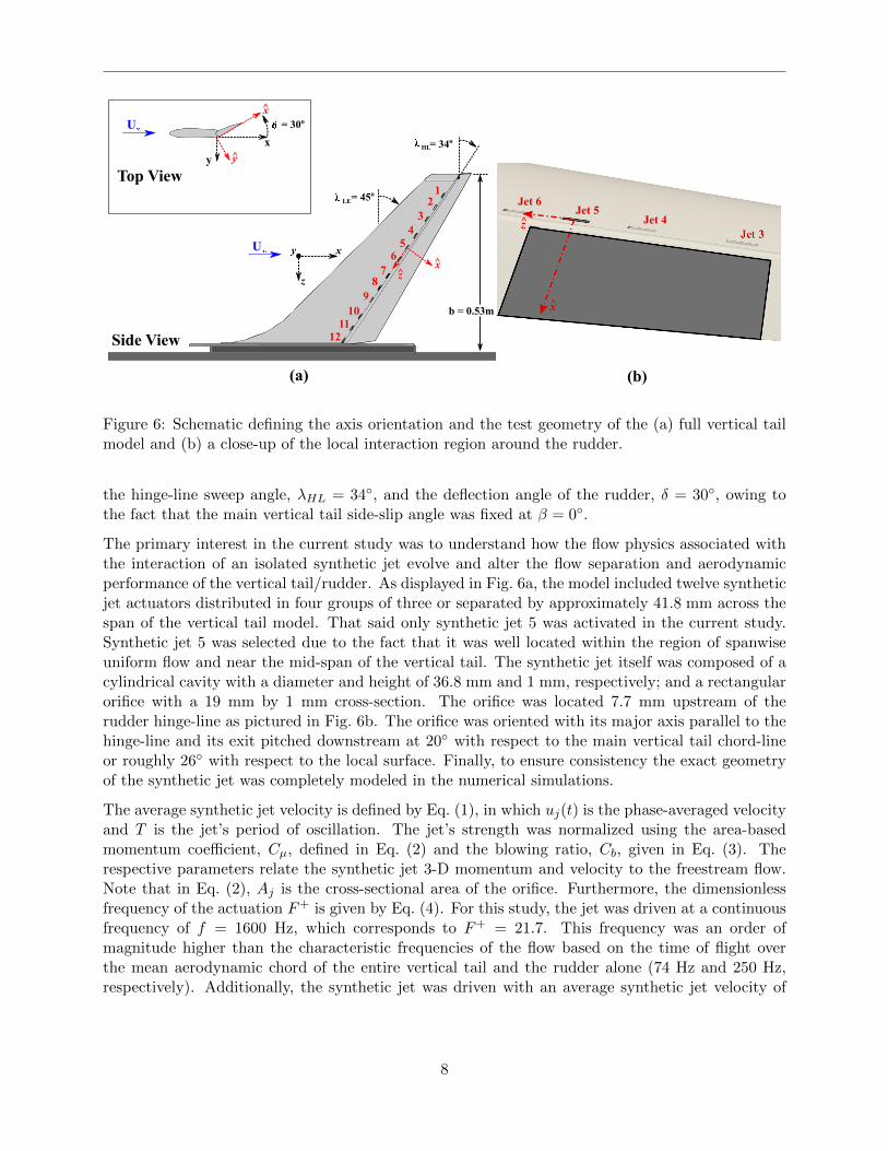
Figure 6: Schematic defining the axis orientation and the test geometry of the (a) full vertical tailmodel and (b) a close-up of the local interaction region around the rudder.
the hinge-line sweep angle, λHL = 34, and the deflection angle of the rudder, δ = 30, owing tothe fact that the main vertical tail side-slip angle was fixed at β = 0.
The primary interest in the current study was to understand how the flow physics associated withthe interaction of an isolated synthetic jet evolve and alter the flow separation and aerodynamicperformance of the vertical tail/rudder. As displayed in Fig. 6a, the model included twelve syntheticjet actuators distributed in four groups of three or separated by approximately 41.8 mm across thespan of the vertical tail model. That said only synthetic jet 5 was activated in the current study.Synthetic jet 5 was selected due to the fact that it was well located within the region of spanwiseuniform flow and near the mid-span of the vertical tail. The synthetic jet itself was composed of acylindrical cavity with a diameter and height of 36.8 mm and 1 mm, respectively; and a rectangularorifice with a 19 mm by 1 mm cross-section. The orifice was located 7.7 mm upstream of therudder hinge-line as pictured in Fig. 6b. The orifice was oriented with its major axis parallel to thehinge-line and its exit pitched downstream at 20 with respect to the main vertical tail chord-lineor roughly 26 with respect to the local surface. Finally, to ensure consistency the exact geometryof the synthetic jet was completely modeled in the numerical simulations.
The average synthetic jet velocity is defined by Eq. (1), in which uj(t) is the phase-averaged velocityand T is the jet’s period of oscillation. The jet’s strength was normalized using the area-basedmomentum coefficient, Cµ, defined in Eq. (2) and the blowing ratio, Cb, given in Eq. (3). Therespective parameters relate the synthetic jet 3-D momentum and velocity to the freestream flow.Note that in Eq. (2), Aj is the cross-sectional area of the orifice. Furthermore, the dimensionlessfrequency of the actuation F+ is given by Eq. (4). For this study, the jet was driven at a continuousfrequency of f = 1600 Hz, which corresponds to F+ = 21.7. This frequency was an order ofmagnitude higher than the characteristic frequencies of the flow based on the time of flight overthe mean aerodynamic chord of the entire vertical tail and the rudder alone (74 Hz and 250 Hz,respectively). Additionally, the synthetic jet was driven with an average synthetic jet velocity of
8

Uj = 17 m/s or a momentum coefficient of Cµ = 0.021% and blowing ratio of Cb = 0.85.
Uj =1
T
∫ T2
0uj(t) dt (1)
Cµ =Uj
2Aj12U∞
2S(2)
Cb =UjU∞
(3)
F+ =fc
U∞(4)
6.2 Experimental Setup
The experiments were conducted at Rensselaer Polytechnic Institute in the open-return low-speedwind tunnel which has a 0.8 m by 0.8 m cross-section and a full working length of 5 m. Themaximum achievable speed was 50 m/s, and the turbulence levels were less than 0.2%. As previouslymentioned, the current study was conducted at a freestream velocity of U∞ = 20 m/s correspondingto a mean chord based Reynolds number of Re = 350, 000. A boundary layer trip, made with 24-gritroughness, was used to ensure a turbulent boundary layer was experimentally present. The tripwas placed at 5% chord on the suction side and 10% chord on the pressure side of the vertical tailmain element. Size and location of the trip were selected based on a detailed study of the pressuredistributions and aerodynamic forces on the model.
Experimentally, the synthetic jet actuator was driven by a clamped piezoelectric disk mounted asone of the end walls of the cylindrical cavity. The synthetic jet’s performance was experimentallycalibrated for a range of frequencies and driving amplitudes (voltages) under quiescent conditionsprior to the wind tunnel tests. Specifically, the calibration focused upon centerline velocity measure-ments made at the jet orifice with a single-element hot-wire probe. To ensure accurate measurementof the peak jet velocity, the probe was located experimentally where the peak velocities of the blow-ing and suction cycles were equal, which approximately corresponded to the orifice exit plane. Theaverage ratio between the blowing and suction peaks was measured to be less than 1.03, which wasdeemed acceptable for the current study.
The aerodynamic forces and moments on the vertical tail were measured using a six-component ATIDelta force/torque sensor. The sensor had a SI-330-30 calibration (ATI Industrial Automation,2013); the drag and side force had a sensing range of 330 N and a resolution of 0.0625 N. Theaccuracy was ±1.25% of the full range, and the sampling frequency was 1 kHz. Data were acquiredfor 30 s for all force measurement tests.
The experimental measurements of the velocity field were made with a stereoscopic particle imagevelocimetry (SPIV) system. This system was composed of a New Wave Solo double-pulsed 120 mJNd:YAG laser and two LaVision Imager Intense thermoelectrically cooled, 12-bit CCD camerasthat each had a resolution of 1376 by 1040 pixels. The vertical tail model was mounted in the windtunnel in a typical configuration, vertically cantilevered from the floor. The cameras were mountedexternal to the wind tunnel test section on the suction side of the vertical tail/rudder assembly andattached to a vibration damped optical table. The laser was also placed on the optical table next to
9

the wind tunnel and illuminated a plane parallel to the rudder hingeline and perpendicular to therudder surface. The two cameras were mounted in a stereoscopic configuration with a separationangle of approximately 45. They were placed upstream of the model at an angle in which the ruddersurface near the hinge-line blocked the strongest intensity laser reflections from the rudder surface.Fixed focal length 60 mm Nikkor lenses were found to provide the appropriate magnification for themeasurement field. Scheimpflug adapters were installed between the lenses and the camera bodiesto realign the focal depth with the oblique viewing angle [31]. Additionally, the cameras lenses wereequipped with 532± 10 nm band pass filters to mitigate the effects of the background illuminationin the room. Calibration was conducted with a LaVision Type 10 calibration plate that for thisconfiguration provided a spatial resolution of 8.4 pixel/mm. This high resolution allowed for theflow physics to be analyzed in great detail.
The laser light sheet was formed with a −20 mm cylindrical lens. It was focused to a waist ofapproximately 2 mm with a variable focal-length lens, and was aligned within the measurementdomain using a three-axis motorized traversing system. The 2 mm waist and a separation timebetween laser pulses of ∆t = 30 µs was used to ensure a sufficient residence time of the tracerparticles as they crossed through the laser plane. The CCD cameras were also mounted on aseparate three-axis traversing system. Both systems consisted of Velmex Bi-Slide traverses, whichhad quoted accuracies of ±4 µm; allowing for the collection of measurements at multiple locationsalong vertical tail span and the rudder chord length. Moreover, a theatrical fog machine thatgenerated water-based smoke particles of O(1 µm) was used to seed the flow. The machine wasplaced in the vicinity of the tunnel’s air inlet, such that there was an even density of particles inthe test section.
The SPIV planes were oriented parallel to the rudder hinge-line and normal to the rudder surface.The measurement domain of a single SPIV plane was located in the hingeline direction betweenz = −126 mm (outboard) and z = 36 mm (inboard) of the synthetic jet orifice. The cameras andlaser were then traversed along the rudder chord, and planes were acquired in 2 mm incrementsfrom x = 13 mm (upstream) to x = 77 mm (downstream). The average SPIV data planes wereassembled into flow volumes via an in-house post-processing program written in Matlab. The greybox in Fig. 6b depicts the actual foot print of the SPIV measurement volume on the surface of therudder.
At each measurement location, a baseline and an actuated data set was collected, each of whichwas composed of 500 double-frame image pairs for each camera (i.e. 2000 individual images). Thedata collection was triggered at a rate which aliased across the synthetic jet actuation cycle. Thismethod allowed for an accurate reconstruction of the time-averaged velocity field, provided that thesynthetic jet actuation frequency was not a multiple of the sampling frequency and that a sufficientnumber of statistics were collected; both of which were verified through analyzing the convergenceof the mean field. The images were processed using Lavision’s DaVis 8.1 software [1]. Specifically,a typical multi-pass scheme, with four-passes of decreasing interrogation window size (from 64 by64 pixels to 32 by 32 pixels) was used with 75% overlap between the interrogation domains. Thein-plane vector components were then stereoscopically reconstructed to provide all three velocitycomponents (u, v, and w) in the two-dimensional SPIV measurement plane.
6.3 Numerical Set-up and Methodology
Special care was brought to the numerical setup in order to match both the physical dimensionsof the geometric model and the physical parameters used in the experiments. Both the 3-D flow
10

computations and the wind tunnel experiments rely on the same CAD model, which ensures thecorrespondence for the dimensions of the stabilizer, rudder, fence, location of the jets on the stabilizerand the inside geometry of the flow control cavities. The chord-based Reynolds number of thecross-flow was also set to 350, 000. The same side-slip angle for the main element and deflectionangle for the rudder as in the experiments were also used. The displacement of the diaphragm ofthe actuator was not modeled in the simulations; instead, a parabolic velocity profile centered onthe active diaphragm (along the radius) with a sinusoidal variation in time was prescribed. Thefrequency of the sinusoidal variation was fixed at 1600 Hz like in the experiments. The amplitude ofthe parabolic velocity profile was set in such a way that the blowing ratio and mass flux computedduring the out-stroke phase of the jet cycle matched with the experiments near the exit plane ofthe jet orifice. Note that an accurate modeling of the flow in the throat of the jet cavity, andsinusoidal actuation via a prescribed velocity boundary condition, have been shown to be essentialto match the experimental conditions [27, 25, 39]. Slip boundary conditions were applied to thefour wind tunnel walls whereas boundaries in front and back were specified as inflow and outflow,respectively. The surfaces composed of the fence, the main element, the rudder, and the flow controlcavity surfaces were considered to be no-slip walls.
The numerical simulations solve the incompressible Navier-Stokes equations. Spatial discretizationwas carried out with a stabilized finite element method (i.e., Streamline/Upwind Petrov-Galerkin(SUPG) method, see Ref. [55]) whereas temporally implicit integration was performed based ona generalized-alpha method (see Ref. [22]). The resulting non-linear algebraic equations were lin-earized to yield a system of equations which were solved using iterative procedures, e.g., GM-RES [36]. Four Newton steps for both the resolution of the Naviers-Stokes equations and turbulencemodel equation (eddy viscosity for delayed detached eddy simulation, DDES [44]) were applied atevery time step in order to ensure a reduction of the non-linear residual of about four orders ofmagnitude on each time step.
Furthermore, mesh resolution was increased in an adaptive fashion since for problems of practicalinterest increasing the mesh resolution to a level necessary for acceptable accuracy in a globallyuniform fashion would introduce extreme demands on the computational resources. In adaptivemesh methods, mesh resolution and configuration are determined and modified in a local fashionbased on the spatial distribution of the solution and errors associated with its numerical approxi-mation (for details see Ref. [38]). Three consecutive meshes were considered in this work which aredenoted hereafter by A0, A1 and A2, where i denotes the adaptation level in Ai. Figure 7 shows theresulting adapted meshes, where the meshes on the left, middle and right panels are respectivelythe initial A0, adapted A1 and A2 meshes. Note that the second adaptation would have included avery large volume of the wake if it were not clipped to reduce the adapted region to the jet 5 plumeas shown in the figure. This approach is consistent with Spalart’s guide to DDES resolution[45].
Every adaptation cycle was applied to a hybrid mesh which includes wedges in the boundary layer,tetrahedra in the core of the domain and, where necessary, pyramids for the transition between thetwo previous topologies. However, wedges and pyramids were tetrahedronized for parallel simula-tions in production mode in order to ensure a better load balance of the computations. Consequently,the initial A0 mesh includes a total of about 500 million tetrahedra. Moreover, a series of threemesh refinement boxes around the airfoil and in the wake of the rudder were applied to the A0mesh as highlighted in Fig. 7c.
A stationary solution with no jet active was first computed on this initial mesh using a RANSmodel [43] with a large time step (∆t = 1.25 × 10⁻³ s). The first adaptation cycle outside the
11

Adaptation cycles:
(a) (b)
(c) (d) (e)
#1 #2
Clip plane of the
adaptation envelope
Figure 7: Initial mesh A0 (c), adapted mesh A1 (d) after the first adaptation cycle, and adaptedmesh A2 (e) after a second adaptation cycle. The mesh resolution is illustrated with an horizontalslice cutting through jet 5. The adaptation envelopes for the first and second adaptation cycles ofthe A1 and A2 meshes are highlighted in red in (a) and (b), respectively. These envelopes includethe tip vortex and wake of the deflected surface for the first adaptation cycle (a). In addition tothese two regions of the domain, the second adaptation envelope also included the jet 5 plume (b).
boundary layer targeted the wake of the rudder. For that purpose, an error identifier based on theeddy viscosity of the RANS model and the PDE residual of the Navier-Stokes equations was usedto determine the associated adaptation envelope inside which adaptation took place, see Fig. 7a.This first adaptation cycle resulted in 780 million tetrahedra in the A1 mesh (see Fig. 7d).
For the A1 and A2 adapted meshes, high fidelity simulations using a hybrid DDES turbulencemodel [44] were carried out for both the baseline and jet 5 configurations. In all cases, implicit timeintegration was performed with a time step ∆t = 5.208 µs, which corresponds to 120 time stepsof constant size in a jet cycle (computations with 180 time-steps in a cycle showed no significantdifferences). It is worth mentioning that DDES is particularly well suited for this application whereflow separation occurs near the junction between the stabilizer and the rudder. Consequently, theDDES model still applied the RANS model on the stabilizer where the flow is fully attached for theconsidered angle of attack. On the other hand the LES model was automatically triggered in theplume of jet 5 and above most of the rudder, downstream of the hinge line where flow separationoccurs. Figure 1 highlights the unsteady vortical structures captured by the DDES model in theLES regions for the jet 5 active case through an isosurface of instantaneous Q criterion colored byspeed. The RANS regions are identified in this figure as regions without small features and/or large,
12
stationary vorticity (e.g., the majority of the stabilizer element and splitter plate) making DDESfar less computationally intensive than pure LES for this geometry.
The second adaptation cycle for both the baseline and jet 5 configurations relied on an error identifierbased on the root mean square of the velocity magnitude, the PDE residual of the Navier-Stokesequations and the distance to the wall (see Figs. 7b and 7e). The resulting A2 mesh includes 1.25billion tetrahedra. In order to limit the cost of the second adaptation cycle, adaptation in the wakeof the rudder was limited to the elements located within one chord distance from the rudder surface,as highlighted in Fig. 7e.
Once a fully developed flow state was reached, average quantities were computed based on samplescollected for 225 cycles on both the A1 and A2 meshes for grid convergence analysis. These 225jet cycles correspond to 10.4 convective periods of the free stream flow over the chord, and 2.7convective periods over the rudder in the direction parallel to the hinge line based on the velocitynear the rudder surface. Time convergence was confirmed through the comparison of the global andlocal statistics over 225 and 105 cycles on the A2 mesh, which showed no significant difference.
These large-scale flow computations could be performed in a reasonable time frame thanks tothe strong scalability of the current flow solver which has been shown to scale up to 786, 432processor-cores (see Ref. [32]), and access to dedicated parallel computing resources. In particular,BlueGene/Q Mira system at the Argonne Leadership Computing Facility (ALCF) was used toperform the numerical computations, where calculations for 225 jet cycles on the A2 adapted meshutilized about 82 hours (in terms of wall-clock time) on 65,536 processor-cores, for a total of 5.4million CPU hours. For post-processing and visualization we used the computer system of Cooleystill at ALCF, along with the visualization tool ParaView from Kitware.
6.4 Findings
In this section, the flow physics associated with the interaction of a single synthetic jet activated inthe region of strong crossflow over the rudder is studied using data from experiments (force balanceand stereo PIV measurements) and numerical simulations. Where possible, the results from thetwo techniques will be compared to cross-validate both methods enabling higher confidence to beachieved in regions where only numerical results are available (e.g., very near the wall). Furthermore,as the primary goal of this study is to understand the large scale effect of the flow control, resultsof the actuated case will be compared to the baseline case to allow a direct assessment of the flowcontrol in each field and scale.
An outline of this section is as follows. In Sec. 6.4.1, the experimental measurements of side force arecompared to CFD. The full tail flow fields from the CFD are compared to the local fields obtainedfrom SPIV in Sec. 6.4.2. From these flow fields, two regions of interest are identified. The firstregion associated with the start of the inboard separation is the focus of Sec. 6.4.3. A strikinglysimilar region just outboard of the activated jet is the study of Sec. 6.4.4. Finally, Sec. 6.4.5 providesan upstream, zoomed view of the SPIV-CFD comparison shown in Sec. 6.4.2.
6.4.1 Side Force
The time-averaged side forces for three experimental cases are shown in Fig. 3 with pink dashedlines for the baseline (no jets active), just jet 5 active, and all 12 jets active. These data sets arefor zero side slip (β = 0) and a rudder deflection of δ = 30. The force time history from theDDES CFD simulations on the adapted meshes for each of the three cases are also shown in the
13

Jet 5
Figure 8: Locations of the SPIV measurement volumes are shown on the vertical tail; inboard region(yellow) and outboard - jet 5 region (green).
same figure with solid lines, color coded to the level of adaptivity. The time averages of these solidlines are shown with dashes. From this figure, a number of conclusions can be drawn. First, theagreement in the average force between the CFD and the experiment is excellent for the baseline.The agreement with all 12 jets active is also excellent. The agreement for the single active jet isquite good, but not as good as the other two. However, it is still well within the uncertainty ofthe experimental measurements. The second conclusion from this figure is that, in terms of sideforce, the CFD is grid independent at the first adaptation since subsequent adaptations (describedin Sec. 6.3) show almost no change in the mean.
Finally, the last conclusion to make is that the side force augmentation from activating a singlejet (i.e. jet 5) is significant compared to actuating all 12 jets. Specifically, the actuation of jet5 alone accounts for approximately 17% of the total side force augmentation by all 12 jets. Thisis approximately double the influence that would be achieved if each of the 12 jets contributedequally to the total side force increase (i.e. 1/12 or 8.3%). Thus, these results again lead to thequestion of “How can a single actuator on a vertical tail model impose such a significant change inthe resulting side force and surrounding flow field?” The following discussion of the computationaland experimental flow fields will serve to thoroughly address and explain this result.
6.4.2 Full Tail Flow Fields
As noted above, SPIV data was collected in a region surrounding jet 5, both with and withoutactuation of jet 5, and in a region inboard near the root of the tail/rudder assembly. In Fig. 8, theSPIV data volume near jet 5 is shown in green while the inboard data volume is shown in yellow. InFig. 9, isosurfaces of time-averaged speed from both of the SPIV volumes are shown first overlaid onthe full isosurface of the time-averaged speed from the CFD at the same values of |~U | = 6, 10, 14,and 18 m/s in the left half of each sub-figure. In the same figure, both the SPIV isosurface and theCFD isosurface are duplicated and off-set in the right half of each sub-figure, so that they can alsobe better compared side-by-side. The agreement at these speeds is remarkable. Below |~U | = 6 m/sthe agreement (not shown) is also good, especially considering the uncertainty in the measurementsat these near wall locations. In Fig. 10, the |~U | = 14 m/s CFD isosurface from the actuated case iscompared to the baseline case. The key finding from this figure is that with a single active jet theflow is not only improved directly in the jet plume, but there is an even stronger improvement tothe flow outboard of the active jet.
14

(c) (d)
(a) (b)
|U| |U|
|U| |U|
Jet 5 Jet 5
Jet 5 Jet 5
Figure 9: Isosurfaces of time-averaged speed, |~U |, from SPIV measurements, near jet 5 (green) andnear root (yellow), overlaid on the full isosurfaces from the CFD for speeds of |~U | = 6 (a), 10 (b),14 (c), and 18 m/s (d). Each panel also shows a duplication and downstream offset of the CFD andSPIV isosurfaces to allow better quantitative comparison of portions blocked by the overlay.
(a) (b)
|U| |U|
Jet 5
Figure 10: Isosurface comparison of time-averaged speed at |~U | = 14 m/s for the baseline (a) andjet 5 active (b) cases.
15

(a) (b)
Jet 5
Figure 11: Comparison of the surface pressure coefficient, Cp, for the baseline (a) and jet 5 active(b) cases.
(a) (b)
Jet 5
Figure 12: Isosurface comparison of vorticity magnitude at |~Ω| = 500 1/s colored by stream-wisevorticity, ~Ωx, for the baseline (a) and jet 5 active (b) cases.
(a) (b)
Jet 5
Figure 13: Comparison of the surface streak patterns colored by wall shear stress magnitude, | ~τw|,for the baseline (a) and jet 5 active (b) cases.
16
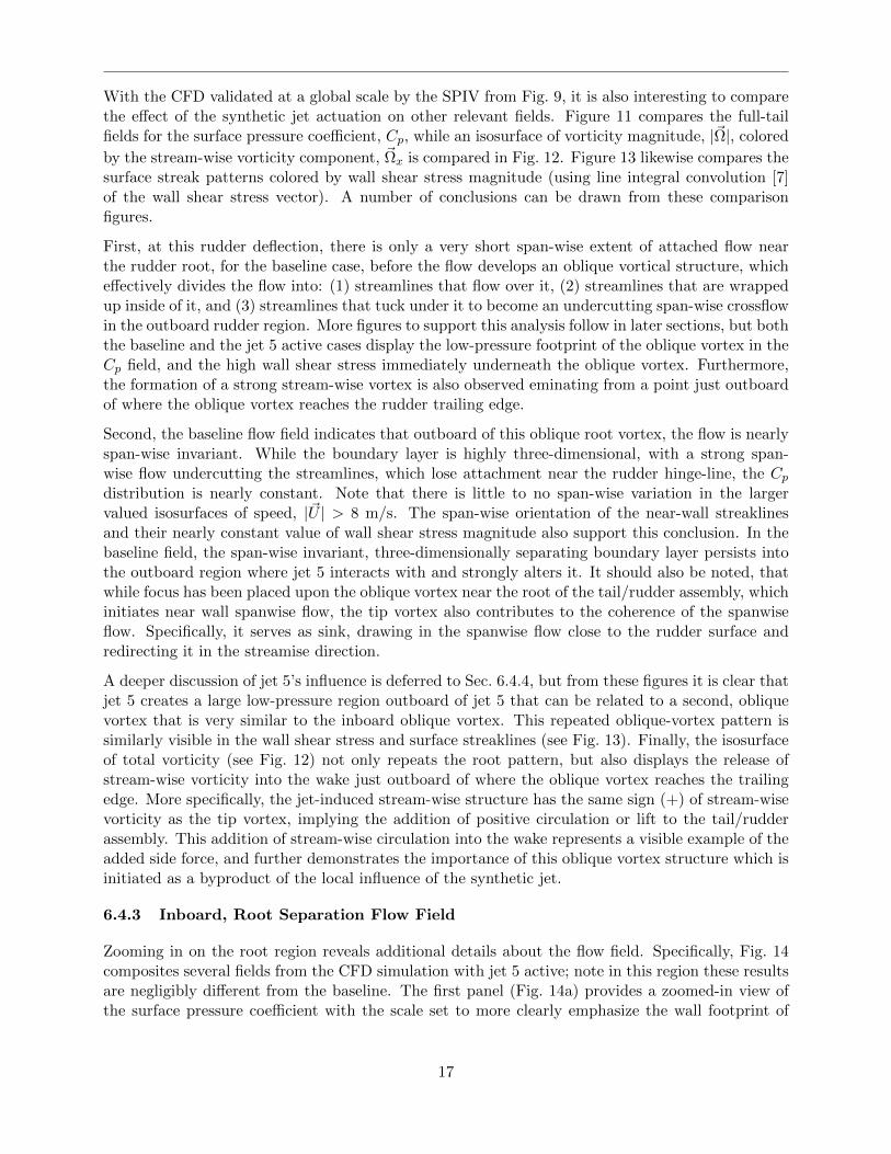
With the CFD validated at a global scale by the SPIV from Fig. 9, it is also interesting to comparethe effect of the synthetic jet actuation on other relevant fields. Figure 11 compares the full-tailfields for the surface pressure coefficient, Cp, while an isosurface of vorticity magnitude, |~Ω|, colored
by the stream-wise vorticity component, ~Ωx is compared in Fig. 12. Figure 13 likewise compares thesurface streak patterns colored by wall shear stress magnitude (using line integral convolution [7]of the wall shear stress vector). A number of conclusions can be drawn from these comparisonfigures.
First, at this rudder deflection, there is only a very short span-wise extent of attached flow nearthe rudder root, for the baseline case, before the flow develops an oblique vortical structure, whicheffectively divides the flow into: (1) streamlines that flow over it, (2) streamlines that are wrappedup inside of it, and (3) streamlines that tuck under it to become an undercutting span-wise crossflowin the outboard rudder region. More figures to support this analysis follow in later sections, but boththe baseline and the jet 5 active cases display the low-pressure footprint of the oblique vortex in theCp field, and the high wall shear stress immediately underneath the oblique vortex. Furthermore,the formation of a strong stream-wise vortex is also observed eminating from a point just outboardof where the oblique vortex reaches the rudder trailing edge.
Second, the baseline flow field indicates that outboard of this oblique root vortex, the flow is nearlyspan-wise invariant. While the boundary layer is highly three-dimensional, with a strong span-wise flow undercutting the streamlines, which lose attachment near the rudder hinge-line, the Cpdistribution is nearly constant. Note that there is little to no span-wise variation in the largervalued isosurfaces of speed, |~U | > 8 m/s. The span-wise orientation of the near-wall streaklinesand their nearly constant value of wall shear stress magnitude also support this conclusion. In thebaseline field, the span-wise invariant, three-dimensionally separating boundary layer persists intothe outboard region where jet 5 interacts with and strongly alters it. It should also be noted, thatwhile focus has been placed upon the oblique vortex near the root of the tail/rudder assembly, whichinitiates near wall spanwise flow, the tip vortex also contributes to the coherence of the spanwiseflow. Specifically, it serves as sink, drawing in the spanwise flow close to the rudder surface andredirecting it in the streamise direction.
A deeper discussion of jet 5’s influence is deferred to Sec. 6.4.4, but from these figures it is clear thatjet 5 creates a large low-pressure region outboard of jet 5 that can be related to a second, obliquevortex that is very similar to the inboard oblique vortex. This repeated oblique-vortex pattern issimilarly visible in the wall shear stress and surface streaklines (see Fig. 13). Finally, the isosurfaceof total vorticity (see Fig. 12) not only repeats the root pattern, but also displays the release ofstream-wise vorticity into the wake just outboard of where the oblique vortex reaches the trailingedge. More specifically, the jet-induced stream-wise structure has the same sign (+) of stream-wisevorticity as the tip vortex, implying the addition of positive circulation or lift to the tail/rudderassembly. This addition of stream-wise circulation into the wake represents a visible example of theadded side force, and further demonstrates the importance of this oblique vortex structure which isinitiated as a byproduct of the local influence of the synthetic jet.
6.4.3 Inboard, Root Separation Flow Field
Zooming in on the root region reveals additional details about the flow field. Specifically, Fig. 14composites several fields from the CFD simulation with jet 5 active; note in this region these resultsare negligibly different from the baseline. The first panel (Fig. 14a) provides a zoomed-in view ofthe surface pressure coefficient with the scale set to more clearly emphasize the wall footprint of
17
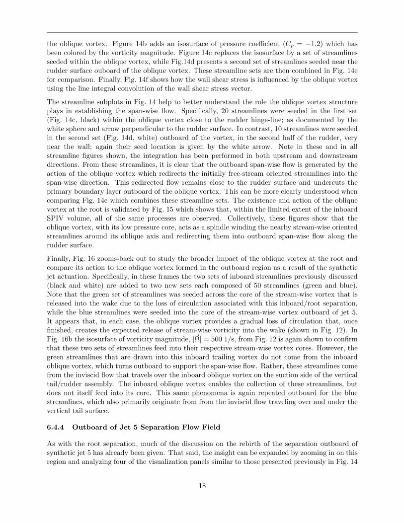
the oblique vortex. Figure 14b adds an isosurface of pressure coefficient (Cp = −1.2) which hasbeen colored by the vorticity magnitude. Figure 14c replaces the isosurface by a set of streamlinesseeded within the oblique vortex, while Fig.14d presents a second set of streamlines seeded near therudder surface ouboard of the oblique vortex. These streamline sets are then combined in Fig. 14efor comparison. Finally, Fig. 14f shows how the wall shear stress is influenced by the oblique vortexusing the line integral convolution of the wall shear stress vector.
The streamline subplots in Fig. 14 help to better understand the role the oblique vortex structureplays in establishing the span-wise flow. Specifically, 20 streamlines were seeded in the first set(Fig. 14c, black) within the oblique vortex close to the rudder hinge-line; as documented by thewhite sphere and arrow perpendicular to the rudder surface. In contrast, 10 streamlines were seededin the second set (Fig. 14d, white) outboard of the vortex, in the second half of the rudder, verynear the wall; again their seed location is given by the white arrow. Note in these and in allstreamline figures shown, the integration has been performed in both upstream and downstreamdirections. From these streamlines, it is clear that the outboard span-wise flow is generated by theaction of the oblique vortex which redirects the initially free-stream oriented streamlines into thespan-wise direction. This redirected flow remains close to the rudder surface and undercuts theprimary boundary layer outboard of the oblique vortex. This can be more clearly understood whencomparing Fig. 14c which combines these streamline sets. The existence and action of the obliquevortex at the root is validated by Fig. 15 which shows that, within the limited extent of the inboardSPIV volume, all of the same processes are observed. Collectively, these figures show that theoblique vortex, with its low pressure core, acts as a spindle winding the nearby stream-wise orientedstreamlines around its oblique axis and redirecting them into outboard span-wise flow along therudder surface.
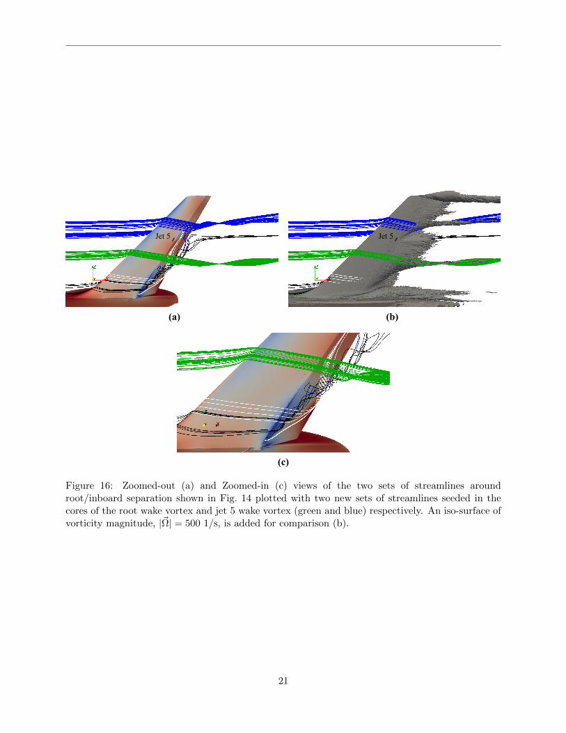
Finally, Fig. 16 zooms-back out to study the broader impact of the oblique vortex at the root andcompare its action to the oblique vortex formed in the outboard region as a result of the syntheticjet actuation. Specifically, in these frames the two sets of inboard streamlines previously discussed(black and white) are added to two new sets each composed of 50 streamlines (green and blue).Note that the green set of streamlines was seeded across the core of the stream-wise vortex that isreleased into the wake due to the loss of circulation associated with this inboard/root separation,while the blue streamlines were seeded into the core of the stream-wise vortex outboard of jet 5.It appears that, in each case, the oblique vortex provides a gradual loss of circulation that, oncefinished, creates the expected release of stream-wise vorticity into the wake (shown in Fig. 12). InFig. 16b the isosurface of vorticity magnitude, |~Ω| = 500 1/s, from Fig. 12 is again shown to confirmthat these two sets of streamlines feed into their respective stream-wise vortex cores. However, thegreen streamlines that are drawn into this inboard trailing vortex do not come from the inboardoblique vortex, which turns outboard to support the span-wise flow. Rather, these streamlines comefrom the inviscid flow that travels over the inboard oblique vortex on the suction side of the verticaltail/rudder assembly. The inboard oblique vortex enables the collection of these streamlines, butdoes not itself feed into its core. This same phenomena is again repeated outboard for the bluestreamlines, which also primarily originate from from the inviscid flow traveling over and under thevertical tail surface.
6.4.4 Outboard of Jet 5 Separation Flow Field
As with the root separation, much of the discussion on the rebirth of the separation outboard ofsynthetic jet 5 has already been given. That said, the insight can be expanded by zooming in on thisregion and analyzing four of the visualization panels similar to those presented previously in Fig. 14
18

(a) (b)
(c) (d)
(e) (f)
Figure 14: Zoomed-in view of the inboard separation region: (a) surface pressure coefficient, Cp,(b) added isosurface of pressure coefficient, Cp = −1.2 (colored by vorticity magnitude), (c) addedstreamlines within oblique vortex (black), (d) added streamlines outboard of the oblique vortex(white), (e) direct comparison of streamline sets, and (d) wall streak pattern colored by wall shearstress, | ~τw|.
19

(a) (b)
(c) (d)
Figure 15: Time-averaged streamlines from CFD (a, c) are compared to time-averaged streamlinesfrom SPIV (b, d) within the inboard volume, overlaid on contours of surface pressure coefficient,Cp, from the CFD.
20
(a) (b)
Jet 5
(c)
Jet 5
Figure 16: Zoomed-out (a) and Zoomed-in (c) views of the two sets of streamlines aroundroot/inboard separation shown in Fig. 14 plotted with two new sets of streamlines seeded in thecores of the root wake vortex and jet 5 wake vortex (green and blue) respectively. An iso-surface ofvorticity magnitude, |~Ω| = 500 1/s, is added for comparison (b).
21

(a) (b)
(c) (d)
1
3
2
Figure 17: Zoomed-in view of the outboard separation region: (a) surface pressure coefficient, Cp,with discussed interaction regions, (b) added isosurface of pressure coefficient, Cp = −1 (colored by
vorticity magnitude, |~Ω| (1/s)), (c) added streamlines seeded within the oblique vortex (black), and(d) wall streak pattern colored by wall shear stress, | ~τw|.
22

for the inboard separation. Figure 17 presents this new figure centered on jet 5 though the isovalueof pressure coefficient in Fig. 17b is now set to Cp = −1. The similar structures present in Figs. 14and 17 confirm that the enhanced circulation over and immediately outboard of jet 5 is, as in thecase of the root, gradually lost through the creation of a second oblique vortex. This oblique vortexonce again converts streamlines oriented in the free-stream direction into span-wise flow close to therudder surface. Note that there are two important differences in this case: (1) jet 5’s actuation and(2) a strong, well-developed span-wise cross-flow that undercuts the boundary layer. Despite thesedifferences the surface pressure, the streamline patterns, and the wall shear stress are strikinglysimilar. Panel (b) represents a noticeable difference with the oblique vortex generated at the rootand presented in Fig. 14b. Specifically, an isosurface of pressure coefficient identifies the vortex coremore clearly than in the inboard (root) separation case, including its expansion and commensuratereduction in vorticity magnitude. This expansion of the vortex is also seen in the streamlines ofFig. 17c, which were seeded across the isosurface of pressure so as to track the streamlines thatwind into the oblique vortex as it expands.
Prior researchers [34, 51, 52] have described how flow control that injects stream-wise momentuminto such a separated flow creates a ‘virtual wall’ or ’fluidic fence’ which obstructs the undercuttingspan-wise flow. While our studies observe the same, we note that, at least in this flow, the lowpressure region created directly by the plume of the jet is significantly smaller than the low pressureregion outboard of the jet. While it is true that the stream-wise momentum provided by the jetdoes partially block the span-wise flow, both the CFD and the SPIV (not shown) indicate that thespan-wise flow is not stopped, rather it is driven closer to the wall as streamlines within the jetplume, and some distance outboard of the jet plume, are able to more closely follow the rudderdeflection.
To better enable the discussion of the jet 5 interaction, three regions are defined based on theirspan-wise position at the hinge-line (see Fig. 17a). The first region is the jet plume, which we taketo be defined by the streamlines that pass within the span-wise extent of jet 5 at the hinge-line.These streamlines are swept outboard and downstream of the hinge-line by the span-wise flow andthe free-stream; which has a significant outboard component due to sweep angle of the verticaltail. We note that in this jet plume region there is only a very small downstream presence of lowpressure generated directly by the added momentum of the jet and its associated Coanda effect.The second region, referred to as the near-jet region, is defined as the streamlines outboard of theplume region, but inboard of the third region which starts where the second oblique vortex begins.Note that this second region may be quite small or even vanish, but conceptually at least, it can bethought of as the region where streamlines are enabled to make a substantial portion of the turnaround the rudder hinge-line without separating. To be clear, in the case shown, this region is ofzero size because all streamlines outboard of the plume do lift off of the surface and wrap aroundthe oblique vortex. We include this region in the discussion because it may be finite size for largerblowing ratios or lower rudder deflection angles.
In the third region, significant turning of the streamlines around the rudder hinge-line creates a tri-angular region of moderately low pressure immediately downstream of the hinge-line and upstreamof the oblique vortex. However, a significantly lower pressure is imposed further downstream by theoblique vortex separation process that is repeated outboard of jet 5 (and was previously discussednear the root). Specifically, the pressure distribution outboard of jet 5 displays a low pressure regioncreated by the footprint of a second, oblique vortex that re-energizes the span-wise flow and has amuch greater impact on side force than the jet plume itself. This finding provides insight into thestrong influence that the span-wise spacing of multiple jets has on the side force; since jets placed
23

too close together will not allow this oblique vortex to fully develop and will thus limit the benefitfrom additional oblique vortices.
In the current case this oblique vortex extends from just outboard of jet 5 past jet 4 before itreaches the rudder trailing edge. This implies that when all 12 jets are activated in the currentconfiguration, neighboring outboard jets will work to directly interfere with the inboard obliquevortices. This interference will reduce the cumulative impact of additional actuators on the sideforce and thus justifies how a single jet alone can have such a large impact. Specifically, in thesingle jet case the oblique vortex is allowed to naturally extend along the rudder in the spanwisedirection for longer distances imposing its maximum influence.
To further understand how activating jet 5 alters the flow, a rake of streamlines seeded at ∆y = 1,2, 4, and 8 mm above and parallel to the hinge-line are plotted in Fig. 18. As before, the seedlocation is given by the white arrow which extends inboard and outboard of jet 5 along the hinge-line. The streamlines are colored by the distance to the wall to clearly show their displacementfrom the surface which can otherwise be difficult to interpret given the three-dimensional nature ofthe geometry and flow. From this figure, it is clear that only a small subset of these streamlines aredrawn into the stream-wise vortex that is released into the wake after the oblique vortex reaches thetrailing edge. The vast majority of streamlines that originate outboard of jet 5 at the ∆y = 1 mmheight (Fig. 18a) are turned outboard before or at the trailing edge. At the ∆y = 2 mm height(Fig. 18b), a few more streamlines are drawn into the stream-wise vortex, but still a large numbercontribute to the span-wise flow. At the ∆y = 4 mm height (Fig. 18c), no streamlines are drawnunder the oblique vortex and a significant number are drawn into the stream-wise vortex. It isworth noting that the boundary layer height near jet 5 is about δ99 = 3 mm so these streamlines arein the inviscid flow, outside of the boundary layer. Finally, at the ∆y = 8 mm height (Fig. 18d), nostreamlines are drawn into the span-wise flow nor the vortex, but there is still significant turningdue to the enhanced circulation created by jet 5. Figure 19 provides a zoomed-in view of the samefour sets of streamlines to better illustrate the spindling or winding of the streamlines at the lowelevations (∆y = 1 and 2 mm off of the wall (Figs. 19a and 19b)) versus the more gradual turningof the inviscid streamlines at ∆y = 4 mm (Fig. 19c) in route to the stream-wise vortex and theeven more gradual turning of the inviscid streamlines that start at ∆y = 8 mm (Fig. 19d) abovethe hinge.
6.4.5 Zoomed Comparison of SPIV and CFD
Much of the above conclusions were based upon CFD fields. To provide a more convincing validationof the CFD fields, Fig. 20 zooms in on the speed isosurfaces, |~U |, with the SPIV data overlaid aspreviously shown in Fig. 9. Even at these zoom levels, the agreement is remarkable, which indicatesthat the CFD and the DDES turbulence model are indeed capable of capturing the time-averagedeffect of synthetic jet-based flow control.
7 Conclusions
The overall conclusion of this report is that, while adaptive, implicit unstructured grid CFD makesuse of very complicated algorithms with formidable scaling challenges, with some effort, they can bemade not only scalable but highly efficient in terms of science provided per CPU hour. Using thesemethods, realistic aircraft components like a vertical tail/rudder assembly complete with active flowcontrol can be simulated accurately at wind tunnel scale and these simulations are on the path toflight scale with Aurora.
24

(a) (b)
(c) (d)
Figure 18: Streamlines colored by the distance to the wall seeded along the line shown which isparallel to the hinge-line and ∆y = 1 (a), 2 (b), 4 (c), and 8 mm (d) above the surface.
25

(a) (b)
(c) (d)
Figure 19: Zoomed-in view of streamlines colored by the distance to the wall seeded along the lineshown which is parallel to the hinge-line and ∆y = 1 (a), 2 (b), 4 (c), and 8 mm (d) above thesurface.
26

(c) (d)
(a) (b)
|U| |U|
|U| |U|
Figure 20: Zoomed-in, upstream view of time-averaged isosurfaces of speed, |~U |, for SPIV measure-ments (grey) overlaid on the CFD (colored) for |~U | = 6 (a), 10 (b), 14 (c), and 18 m/s (d) when jet5 is active.
27

A second, and equally important conclusion relates to the fact that these simulations have unlockednew understanding of how flow control works in these complicated flows. In this report we have alsodetailed our validation efforts where a carefully coordinated experimental and computational studyof a vertical tail/rudder assembly with a δ = 30 rudder deflection was performed and described.Both the baseline and a single active synthetic jet cases were compared to provide excellent cross-validation of the force and large-scale time-averaged flow fields. From these fields, insight was gainedregarding the separation process and its role in lift or side-force generation.
Specifically, the first major finding was the identification of an initial root separation that forms avortex that is oblique to the rudder and provides a spindle-like mechanism to re-direct free-stream-oriented streamlines within the boundary layer into a span-wise flow that fills the gap under theoutboard separating streamlines. This oblique vortex originates at the point of initial separationand, through an oblique line, travels downstream and outboard until it reaches the trailing edgewhere it is turned outboard. It is hypothesized that this oblique vortex provides a smooth transi-tion between the high-circulation attached flow inboard and the significantly lower circulation flowoutboard. Indeed it was observed that the stream-wise vortex released in the wake that is expectedfrom a large change in circulation occurs just outboard of where this oblique vortex reaches thetrailing edge. It was confirmed that, while this vortex facilitates the transition of circulation, itscore does not directly feed into the stream-wise vortex, rather it turns the streamlines that do.
A second major finding of this study is that outboard of the oblique vortex a nearly span-wiseinvariant flow is created that undercuts the separating streamlines over a significant portion of thespan. As a result, the surface pressure gradient is almost zero (both span-wise and stream-wise)over a large portion of the rudder surface. The wall shear stress is also nearly constant in bothmagnitude and direction throughout this region. Therefore in this region, a single jet acts on arelatively simple three-dimensional boundary layer, considering the complex geometry that createsit (e.g., swept and tapered vertical tail with a δ = 30 rudder deflection). Indeed this was thepurpose in selecting synthetic jet 5 for this study.
The third major finding in this study is that DDES is capable of predicting not only the change inside force, but the actual side force of the baseline and the active jet configurations (1 and 12 jetsactive). Furthermore, it was shown capable of predicting the isosurfaces of speed, |~U |, which wereexperimentally validated from SPIV measurements around the active jet.
The fourth major finding from this study was that, while it is true that the direct action of the syn-thetic jet is to create a virtual fence or wall by injecting stream-wise momentum, the vast majorityof the area of improved surface pressure distribution is outboard of the jet. This improvement wasobserved from two sources. The first source, which we refer to as near-jet improvement, relates tothe streamlines just outboard of the active jet that are turned by both the synthetic jet and theoutboard oblique vortex to follow closer to the rudder surface. The term closer is used because thejet does not actually reattach the flow, rather, the span-wise flow is forced closer to the wall. Thegreater impact on surface pressure distribution (and thus side force) comes from a rebirth of thespan-wise separation which produced a second oblique vortex, in a manner that is strikingly similarto the inboard (root) separation. However, in this case, the second oblique vortex originates wherethe active jet is no longer able to turn the streamlines and continues obliquely downstream andoutboard until it connects this new separation to the trailing edge. This vortex is quite strong andthe pressure drop that it creates provides a large, low pressure footprint on the surface of the rudder,thus providing a majority contribution to the increase in side force. To the authors’ knowledge, thisis the first time that this side force generation mechanism has been documented and explained–that is, to show that the majority of the side force enhancement is created by the structure that
28

re-established the span-wise separated flow as opposed the relatively small (in span and stream-wiseextent) region within the jet plume. This finding provides insight into the strong influence of span-wise jet spacing since jets placed too close together will diminish this benefit. While the majorityof the fields that illustrate this process are obtained from CFD, the thorough validation againstcarefully matched experimental conditions and the verification through a series of adapted mesheswith negligible change in observed quantities gives high confidence in these conclusions.
Acknowledgements
The authors acknowledge The Boeing Company for full support of the experimental investigationsand partial support of the computational simulations. An award of computer time was providedby the Innovative and Novel Computational Impact on Theory and Experiment (INCITE) programand the Theta Early Science Program. This research used resources of the Argonne LeadershipComputing Facility, which is a DOE Office of Science User Facility supported under ContractDE-AC02-06CH11357. Specifically, the production runs were done on Mira and Theta while thepost-processing was done on Cooley. This work also utilized the Janus supercomputer, which issupported by the National Science Foundation (award number CNS-0821794) and the Universityof Colorado Boulder. The Janus supercomputer is a joint effort of the University of ColoradoBoulder, the University of Colorado Denver and the National Center for Atmospheric Research.Specifically, these resources were used in mesh generation and pre-processing. The SCOREC-coremesh partitioning and adaptation tools used in this research were supported by the U.S. Departmentof Energy, Office of Science, Office of Advanced Scientific Computing Research, under award DE-SC00066117 (FASTMath SciDAC Institute). M. Rasquin was funded by an Early Science Programpost-doctoral fellowship from the Argonne Leadership Computing Facility for some part of thiswork. The solutions presented here made use of software components provided by Altair Engineering(Acusim), Simmetrix (MeshSim and SimModeler), and Kitware (ParaView).
29

References
[1] DaVis FlowMaster Manuals for DaVis 8.1. Gottingen, Germany, 2012.
[2] Frederik Alauzet, Xiangrong Li, E. Seegyoung Seol, and Mark S. Shephard. Parallel anisotropic3d mesh adaptation by mesh modification. Engineering with Computers, 21(3):247–258, jan2006.
[3] M. Amitay, B.L. Smith, and A. Glezer. Aerodynamic Flow Control Using Synthetic Jet Tech-nology. AIAA Paper, 208, 1998.
[4] Satish Balay, Jed Brown, Matt Knepley, Lois Curfman McInnes, Barry F. Smith, and HongZhang. PETSc homepage. http://www.mcs.anl.gov/petsc, 2016.
[5] I.A. Bolotnov, K.E. Jansen, D.A. Drew, A. A. Oberai, R.T. Lahey Jr., and M.Z. Podowski.Detached direct numerical simulations of two-phase bubbly channel flow. Intl. J. of MultiphaseFlows, 37(6):647–659, 2011.
[6] A. N. Brooks and T. J. R. Hughes. Streamline upwind / Petrov-Galerkin formulations for con-vection dominated flows with particular emphasis on the incompressible Navier-Stokes equa-tions. Comp. Meth. Appl. Mech. Engng., 32:199–259, 1982.
[7] Brian Cabral and Leith Casey Leedom. Imaging vector fields using line integral convolution.In Proceedings of the 20th annual conference on Computer graphics and interactive techniques,pages 263–270. ACM, 1993.
[8] K.C. Chitale, O. Sahni, M.S. Shephard, S. Tendulkar, and K.E. Jansen. Anisotropic adaptationfor transonic flows with turbulent boundary layers. AIAA Journal, 53, 2015.
[9] Kedar C Chitale, Michel Rasquin, Onkar Sahni, Mark S Shephard, and Kenneth E Jansen.Anisotropic boundary layer adaptivity of multi-element wings. In 52nd Aerospace SciencesMeeting (SciTech). AIAA paper 2014-0117, 2014.
[10] J. Fang, M. Rasquin, and I.A. Bolotnov. Interface tracking simulations ofbubbly flows in pwr relevant geometries. Nuclear Engineering and Design,http://dx.doi.org/10.1016/j.nucengdes.2016.07.002, 2016.
[11] A. Glezer and M. Amitay. Synthetic Jets. Annual Review of Fluid Mechanics, 34(1):503–529,2002.
[12] The Open Group. XSI Shared memory facility. The Open Group Base Specifications Issue 7,2013 edition. http://pubs.opengroup.org/onlinepubs/9699919799/ basedefs/sys shm.h.html.
[13] Torsten Hoefler, James Dinan, Darius Buntinas, Pavan Balaji, Brian Barrett, Ron Brightwell,William Gropp, Vivek Kale, and Rajeev Thakur. Mpi + mpi: a new hybrid approach to parallelprogramming with mpi plus shared memory. Computing, 95(12):1121 – 1136, 2013.
[14] T. J. R. Hughes, L. Mazzei, and K. E. Jansen. Large-eddy simulation and the variationalmultiscale method. Computing and Visualization in Science, 3:47–59, 2000.
[15] Dan Ibanez, Ian Dunn, and Mark S Shephard. Hybrid MPI-thread parallelization of adaptivemesh operations. Parallel Computing, 52(2):133–143, 2016.
[16] Dan Ibanez and Mark S. Shephard. Modifiable array data structures for mesh topology. SIAMJournal on Scientific Computing, 2016. submitted.
30
[17] Dan Ibanez and Mark S. Shephard. Portably performant mesh adaptation. Engineering withComputers, 2016. submitted.
[18] Daniel A Ibanez, E Seegyoung Seol, Cameron W Smith, and Mark S Shephard. Pumi: Parallelunstructured mesh infrastructure. ACM Transactions on Mathematical Software (TOMS),42(3):17, 2016.
[19] K. E. Jansen. Unstructured grid large eddy simulation of flow over an airfoil. In AnnualResearch Briefs, pages 161–173, NASA Ames / Stanford University, 1994. Center for TurbulenceResearch.
[20] K. E. Jansen. A stabilized finite element method for computing turbulence. Comp. Meth. Appl.Mech. Engng., 174:299–317, 1999.
[21] K. E. Jansen and A. E. Tejada-Martınez. An evaluation of the variational multiscale model forlarge-eddy simulation while using a hierarchical basis. (2002-0283), Jan. 2002.
[22] K. E. Jansen, C. H. Whiting, and G. M. Hulbert. A generalized-α method for integrating thefiltered Navier-Stokes equations with a stabilized finite element method. Comp. Meth. Appl.Mech. Engng., 190:305–319, 1999.
[23] K.E. Jansen. Unstructured grid large eddy simulation of wall bounded flow. In Annual Re-search Briefs, pages 151–156, NASA Ames / Stanford University, 1993. Center for TurbulenceResearch.
[24] Kenneth Jansen. https://github.com/phasta.
[25] Rupesh B Kotapati, Rajat Mittal, and Louis N Cattafesta III. Numerical study of a transitionalsynthetic jet in quiescent external flow. Journal of Fluid Mechanics, 581:287–321, 2007.
[26] N. Liu, J. Fu, C.D. Carothers, O. Sahni, K.E. Jansen, and M.S. Shephard. Massively paralleli/o for partitioned solver systems. Parallel processing letters, 20(4):377–395, 2010.
[27] S. Muppidi and K. Mahesh. Study of trajectories of jets in crossflow using direct numericalsimulations. Journal of Fluid Mechanics, 530:81–100, 2005.
[28] S. Nagrath, K. E. Jansen, and R. T. Lahey. Three dimensional simulation of incompressibletwo phase flows using a stabilized finite element method and the level set approach. Comp.Meth. Appl. Mech. Engng., 194(42-44):4565–4587, 2005.
[29] S. Nagrath, K. E. Jansen, R. T. Lahey, and I. Akhatov. Hydrodynamic simulation of air bubbleimplosion using a fem based level set approach. Journal of Computational Physics, 215:98–132,2006.
[30] Aleksandr Ovcharenko, Kedar C. Chitale, Onkar Sahni, Kenneth E. Jansen, and Mark S.Shephard. Parallel adaptive boundary layer meshing for cfd analysis. In Xiangmin Jiao andJean-Christophe Weill, editors, Proceedings of the 21st International Meshing Roundtable, pages437–455. Springer Berlin Heidelberg, 2013.
[31] Arun K Prasad. Stereoscopic particle image velocimetry. Experiments in fluids, 29(2):103–116,2000.
[32] M. Rasquin, C. Smith, K. Chitale, E.S. Seol, B.A. Matthews, J.L. Martin, O. Sahni, R.M. Loy,M.S. Shephard, and K.E. Jansen. Scalable implicit flow solver for realistic wing simulationswith flow control. Computing in Science and Engineering, 16(6):13–21, 2014.
31

[33] M. Rasquin, C. Smith, K Chitale, S. Seol, B.A. Matthews, J.L. Martin, O. Sahni, R.M. Loy,M.S. Shephard, and K.E. Jansen. Scalable fully implicit finite element flow solver with applica-tion to high-fidelity flow control simulations on a realistic wing design. Computing in Scienceand Engineering, 16(6):13–21, 2014.
[34] Nicholas Rathay, Matthew Boucher, Michael Amitay, and Edward Whalen. Performance en-hancement of a vertical stabilizer using synthetic jet actuators: Non-zero sideslip. In AIAAPaper 2012-2657, New Orleans, LA, 2012. 6th AIAA Flow Control Conference, Fluid Dynamicsand Co-located Conferences, American Institute of Aeronautics and Astronautics.
[35] J.M. Rodriguez, O. Sahni, R.T. Lahey Jr., and K.E. Jansen. A parallel adaptive mesh methodfor the numerical simulation of multiphase flows. Computers and Fluids, 87:115–131, 2013.
[36] Y. Saad. Iterative methods for sparse linear systems. PWS Pub. Co., 1996.
[37] Y. Saad and M.H. Schultz. GMRES: A generalized minimal residual algorithm for solvingnonsymmetric linear systems. SIAM Journal of Scientific and Statistical Computing, 7:856–869, 1986.
[38] O. Sahni, J. Mueller, K.E. Jansen, M.S. Shephard, and C.A. Taylor. Efficient anisotropicadaptive discretization of cardiovascular system. Comp. Meth. Appl. Mech. Engng., 195(41-43):5634–5655, 2006.
[39] Onkar Sahni, Joshua Wood, Kenneth E Jansen, and Michael Amitay. Three-dimensional in-teractions between a finite-span synthetic jet and a crossflow. Journal of Fluid Mechanics,671:254–287, 2011.
[40] Cameron W. Smith, Michel Rasquin, Dan Ibanez, Kenneth E. Jansen, and Mark S. Shephard.Improving unstructured mesh partitions for multiple criteria using mesh adjacencies. SIAMJournal on Scientific Computing, In Review, 2016.
[41] Cameron W. Smith, Michel Rasquin, Dan Ibanez, Mark S. Shephard, and Kenneth E. Jansen.Partition improvement to accelerate extreme scale cfd. SIAM Journal on Scientific Computing,in preparation, 2015.
[42] Cameron W Smith, Steven Tran, Onkar Sahni, Farhad Behafarid, Mark S Shephard, andRaminderjeet Singh. Enabling hpc simulation workflows for complex industrial flow problems.In Proceedings of the 2015 XSEDE Conference: Scientific Advancements Enabled by EnhancedCyberinfrastructure, page 41. ACM, 2015.
[43] Philippe R Spalart and Steven R Allmaras. A one equation turbulence model for aerodinamicflows. AIAA journal, 94, 1992.
[44] Philippe R Spalart, Shur Deck, ML Shur, KD Squires, M Kh Strelets, and A Travin. A newversion of detached-eddy simulation, resistant to ambiguous grid densities. Theoretical andcomputational fluid dynamics, 20(3):181–195, 2006.
[45] P.R. Spalart. Young person’s guide to detached-eddy simulation grids. Technical report,Technical Report NASA/CR-2001-211032, 2001.
[46] Srinivas Sridharan, James Dinan, and Dhiraj D Kalamkar. Enabling efficient multithreaded mpicommunication through a library-based implementation of mpi endpoints. In High PerformanceComputing, Networking, Storage and Analysis, SC14: International Conference for, pages 487–498. IEEE, 2014.
32

[47] A. E. Tejada-Martınez and K. E. Jansen. Spatial test filters for dynamic model large-eddysimulation on finite elements. Communications in Numerical Methods in Engineering, 19:205–213, 2003.
[48] A. E. Tejada-Martınez and K. E. Jansen. A dynamic Smagorinsky model with dynamic deter-mination of the filter width ratio. Physics of Fluids, 16:2514–2528, 2004.
[49] A. E. Tejada-Martınez and K. E. Jansen. On the interaction between dynamic model dissipationand numerical dissipation due to streamline upwind/Petrov-Galerkin stabilization. Comp.Meth. Appl. Mech. Engng., 194(9-11):1225–1248, 2005.
[50] A. E. Tejada-Martınez and K. E. Jansen. A parameter-free dynamic subgrid-scale model forlarge-eddy simulation. Comp. Meth. Appl. Mech. Engng., 195(23):2919–2938, 2006.
[51] P. Tewes and L. Taubert. Control of separation on a swept wing using fluidic oscillators. InAIAA Paper 2015-0783, Kissimmee, FL, 2015. 53rd AIAA Aerospace Sciences Meeting, AIAASciTech Forum, American Institute of Aeronautics and Astronautics.
[52] Philipp Tewes, Lutz Taubert, and Israel J. Wygnanski. On the effect of sweep on separationcontrol. In AIAA Paper 2014-2513, Atlanta, GA, 2014. 7th AIAA Flow Control Conference,AIAA AVIATION Forum, American Institute of Aeronautics and Astronautics.
[53] A.M. Thomas, J. Fang, J. Feng, and I.A. Bolotnov. Estimation of shear-induced lift force inlaminar and turbulent flows. Nuclear Technology, 190:274–291, 2015.
[54] Various. http://www.mcs.anl.gov/research/projects/codes/.
[55] C. H. Whiting and K. E. Jansen. A stabilized finite element method for the incompressibleNavier-Stokes equations using a hierarchical basis. International Journal of Numerical Methodsin Fluids, 35:93–116, 2001.
[56] C. H. Whiting, K. E. Jansen, and S. Dey. Hierarchical basis in stabilized finite element methodsfor compressible flows. Comp. Meth. Appl. Mech. Engng., 192(47-48):5167–5185, 2003.
[57] M. Zhou, O. Sahni, T. Xie, M.S. Shephard, and K.E. Jansen. Unstructured mesh partitionimprovement for implicit finite element at extreme scale. Journal of Supercomputing, 59(3):1218– 28, 2012/03/.
[58] Xiaomin Zhu, Junchao Zhang, Kazutomo Yoshii, Shigang Li, Yunquan Zhang, and Pavan Bal-aji. Analyzing mpi-3.0 process-level shared memory: A case study with stencil computations.2015 15th IEEE/ACM International Symposium on Cluster, Cloud & Grid Computing, page1099, 2015.
33

Argonne Leadership Computing FacilityArgonne National Laboratory9700 South Cass Avenue, Bldg. #240Argonne, IL 60439
www.anl.gov
Argonne National Laboratory is a U.S. Department of Energy
laboratory managed by UChicago Argonne, LLC