extreme chaos: flexible and efficient all-to-all data ... · data aggregation for wireless sensor...
TRANSCRIPT

Delft University of TechnologyMaster’s Thesis in Embedded Systems
Extreme Chaos: Flexible and EfficientAll-to-All Data Aggregation for Wireless
Sensor Networks
Dimitrios Chronopoulos


Extreme Chaos: Flexible and Efficient All-to-All
Data Aggregation for Wireless Sensor Networks
Master’s Thesis in Embedded Systems
Embedded Software SectionFaculty of Electrical Engineering, Mathematics and Computer Science
Delft University of TechnologyMekelweg 4, 2628 CD Delft, The Netherlands
Dimitrios [email protected]
28th January 2016

AuthorDimitrios Chronopoulos ([email protected])
TitleExtreme Chaos: Flexible and Efficient All-to-All Data Aggregationfor Wireless Sensor Networks
MSc presentation9th February 2016
Graduation CommitteeProf. Dr. K.G. Langendoen Delft University of TechnologyProf. Ir. Dr. D. H. J. Epema Delft University of TechnologyMarco Antonio Zuniga Zamalloa Delft University of TechnologyMarco Cattani Delft University of Technology

“Rick: Sometimes science is a lot more art than it is science. A lot ofpeople do not get that...” – ”Rick and Morty” by Justin Roiland & Dan
Harmon, 2013


Preface
This thesis presents the work I performed in the Embedded Software Grouptowards obtaining my master’s degree in Embedded Systems. During my 8years in academia I have been involved in a wide range of topics in computerscience and networking. My natural inclination towards practical projects,and also my desire to challenge myself and expand my knowledge, led meto the Embedded Software Group. There, I was able to find a project thatcould make use of my prior education, introduce me to the field of WirelessSensor Networks and its peculiar challenges, and give me the opportunity touse my skills in order to meaningfully contribute to the scientific community.My thesis provided all this, while being a project with a prevalent practicalnature due to implementation requirements and device restrictions. I hopethat this work will allow me to further delve in WSNs in the future becauseI believe it is a field with many potential real-world applications.
I would like to thank a great number of people for the help I received fromthem during this thesis. First and foremost, I feel the need to expressmy sincerest gratitude and respect to my daily advisor and friend, MarcoCattani. He is the one whose ideas and projects inspired me to join theEmbedded Software Group and the one who brought the basis of this projectto my attention. Thanks to his guidance and support I was able to conductmy work smoothly, by always having a precise goal in mind. Besides myadvisor, I would like to thank professor Marco Antonio Zuniga Zamalloa,who acted as my supervising professor, for accepting me as his student andfor the valuable insight and feedback he gave me. Additionally, my thanksgoes to the creators of the Chaos protocol, Olaf Landsiedel et al, sincewithout their work this thesis would not have been possible. Last but notleast, I thank all the members of the Embedded Software group for makingthe experience of carrying out a thesis enjoyable and interesting, and ofcourse my family for giving me the opportunity to make it this far.
Dimitrios Chronopoulos
Delft, The Netherlands28th January 2016
v


Contents
Preface v
1 Introduction 11.1 Gathering Data in WSNs . . . . . . . . . . . . . . . . . . . . 21.2 Data Aggregation . . . . . . . . . . . . . . . . . . . . . . . . . 3
2 Related Work 52.1 A taxonomy of solutions . . . . . . . . . . . . . . . . . . . . . 6
2.1.1 The 3 dimensions of protocols . . . . . . . . . . . . . . 62.1.2 Types of aggregates . . . . . . . . . . . . . . . . . . . 8
2.2 Shortest-path routing . . . . . . . . . . . . . . . . . . . . . . 92.3 Opportunistic and Multi-path routing . . . . . . . . . . . . . 102.4 Synchronized flooding-based protocols . . . . . . . . . . . . . 11
3 Chaos: all-to-all data aggregation 133.1 On choosing Chaos . . . . . . . . . . . . . . . . . . . . . . . 133.2 Inside Chaos . . . . . . . . . . . . . . . . . . . . . . . . . . . 14
3.2.1 Two synchronization layers . . . . . . . . . . . . . . . 143.2.2 The Chaos round . . . . . . . . . . . . . . . . . . . . . 15
3.3 Chaos’ problems and limitations . . . . . . . . . . . . . . . . 183.3.1 Scalability . . . . . . . . . . . . . . . . . . . . . . . . . 183.3.2 Resilience to dynamics . . . . . . . . . . . . . . . . . . 183.3.3 Efficiency . . . . . . . . . . . . . . . . . . . . . . . . . 193.3.4 Aggregate type limitations . . . . . . . . . . . . . . . 21
4 Extreme Chaos 234.1 Estimation vector . . . . . . . . . . . . . . . . . . . . . . . . . 23
4.1.1 Replacing the flags-field . . . . . . . . . . . . . . . . . 244.1.2 A vector of size estimators . . . . . . . . . . . . . . . . 24
4.2 Flow control . . . . . . . . . . . . . . . . . . . . . . . . . . . . 264.2.1 Exponentially decaying ”back-off” probability . . . . . 274.2.2 Self-tuned initial probability P0 . . . . . . . . . . . . . 30
4.3 Inside Extreme Chaos . . . . . . . . . . . . . . . . . . . . . . 314.3.1 Initialization . . . . . . . . . . . . . . . . . . . . . . . 31
vii

4.3.2 Aggregation . . . . . . . . . . . . . . . . . . . . . . . . 314.3.3 Termination . . . . . . . . . . . . . . . . . . . . . . . . 32
4.4 Complex aggregates . . . . . . . . . . . . . . . . . . . . . . . 34
5 Evaluation 375.1 Testbeds and Evaluation Metrics . . . . . . . . . . . . . . . . 375.2 Scalability . . . . . . . . . . . . . . . . . . . . . . . . . . . . . 385.3 Reliability and speed . . . . . . . . . . . . . . . . . . . . . . . 395.4 Flexibility to network dynamics . . . . . . . . . . . . . . . . . 445.5 Estimation of duplicate sensitive aggregates . . . . . . . . . . 47
6 Discussion 496.1 Chaos: A distributed control system? . . . . . . . . . . . . . . 496.2 Extreme channel hopping . . . . . . . . . . . . . . . . . . . . 51
7 Conclusions 53

Chapter 1
Introduction
Wireless sensor networks (WSNs) are systems of collaborating devices (i.e.sensor nodes) with the goal of retrieving information about the area in whichthey are deployed. WSNs provide a broad range of applications, usually inthe fields of environmental monitoring, health and security.
WSNs exhibit unique traits that distinguish them from classic communic-ation networks (e.g. wired networks). In particular, they are characterizedby the following four properties [1]:
• Inherently Dynamic. WSNs have a volatile topology and networksize, because nodes often become disconnected due to temporary orfatal faults, and node mobility. The link quality is also not stableand can be affected by natural phenomena (obstacles, environmentalconditions), making a connection between two nodes unpredictable.
• Dense. The questionable availability of WSN nodes, often imposesthe deployment of additional nodes to dependably achieve sufficientcoverage of the target area. These potentially redundant nodes in-crease the network’s density. The high density of WSNs poses chal-lenges in the coordination of their sensor nodes, which in turn makesthe collection of sensory data costly in both time and energy.
• Energy Constraint. WSN nodes are usually battery powered withthe main energy expense coming from operating their radio. As such,it is common practice for WSN nodes to duty cycle their radios toavoid depleting their batteries very quickly. Duty cycling the radiosmeans that nodes switch their radio transceiver on and off periodically.The duty cycle is the fraction of time the radio is active during thison-off cycle. Typically, low duty cycles are desired to conserve as muchenergy as possible. However, there is a limit to how small duty cyclescan be, as nodes need to be available often enough for communicationto be possible.
1

It is therefore very important to employ efficient scheduling schemesthat allow pairs of adjacent nodes to be simultaneously available. Oth-erwise, a transmitting node has to keep attempting to send the samepacket multiple times (wasting energy) until the desired receiving nodeactivates its radio. Thus, striking a balance between low duty cyclesand efficient communication (in order to extend the lifetime of WSNs)is very difficult.
• Medium Sharing. In Wireless networks, nodes use the same commu-nication medium (the electromagnetic spectrum) and need to employMedium Access Control (MAC) methods that allows them to share itin an efficient manner. Although this is true for other types of networkstoo, in WSNs usually more nodes can interfere with one another; inpractice packets generated from nodes in a 2-hop neighborhood couldcause a collision. Combined with the tendency to deploy WSN nodesin dense topologies, this property means that communication in WSNis truly challenging.
Throughout this work we will show how these four properties decisivelyaffect the performance of WSNs, and how they lead to specific choices indesigning protocols for the communication of network nodes.
1.1 Gathering Data in WSNs
The purpose of WSNs is to sense the environment and forward every node’sdata to the sink, a special node that possesses the capability to deliver thecollected data to the overlying sensing application. Since the sink acts as thegateway, the goal of many communication protocols is to optimally route allsensor readings to it.
However, routing information to the network sink is difficult due to thevolatile nature of wireless links. This volatile nature prevents maintaininga constant flow of data (high network throughput) because nodes need tore-discover paths towards the sink. Such network discovery steps have asignificant cost as they increase network traffic and delay the routing ofsensor values. Thus, collecting every sensor’s value can be a time and energyconsuming process.
This in turn leads to two problems. First, the sensing application be-comes slower and less responsive as the time required for communicationbecomes the system’s bottleneck and sensor values are collected at slowerrates. Second, the network’s lifetime decreases since a great deal of poweris consumed on radio operation. In order to alleviate these problems andachieve considerable savings, the paradigm of data aggregation has beenutilized by WSN researchers.
2

1.2 Data Aggregation
The main idea behind data aggregation is to combine information whilerouting sensor values towards the sink, and as a result substantially reducethe total amount of data (in terms of bytes) forwarded. In effect, data ag-gregation shifts the nature of communication from an address-centric focus,which cares for point-to-point interactions between the sources and the sink,to a more data-centric one, whose purpose is to ensure that the sink receivesonly the necessary information. With aggregation, the propagation of re-dundant values is limited, saving precious communication time and energy.This great benefit is the main reason why this paradigm has become a corebuilding block of many WSN protocols [17].
Aggregates can report the necessary insight residing in sensor readings ina concise form. For some applications for example, it might be enough toknow the extremes (MIN, MAX), or the SUM of the sensed values. Furthermore,aggregates can represent global networks properties, and thus allow for aswift gathering of statistics about the performance of the network protocols(loss rates, packet count), or the overall status of the network (energy level).
Due to their versatility, acquiring knowledge of global aggregates withinshort intervals is enough to cover the primary functionality of many sensingapplications. It is thus of great importance to develop methods capable ofproviding such aggregates quickly and with a low energy overhead.
This thesis is motivated by the aforementioned benefits of aggregation andthe need to design protocols that respect the four core WSN properties wedescribed earlier. We base our approach on a synchronous, flooding-based,communication primitive that relies on the capture effect to perform all-to-all data aggregation. We combine it with a gossip technique, which relies onorder statistics, to make it flexible to network dynamics, and a preemptiveflow control policy to resolve issues related to density. The resulting outcomeis an integrated solution we name Extreme Chaos, that is capable of ag-gregating the network’s data more efficiently, and in more ways (computinga greater variety of aggregate-types1) than existing mechanisms.
This thesis is organized in the following manner: Chapter 2 provides an over-view of the related work and the motivation behind the key design choices ofour protocol. Chapter 3 describes Chaos [19], which is the protocol on topof which our work expands, and also presents its main shortcomings and thereasons behind them. Chapter 4 introduces our solution, Extreme Chaos,and gives an in-depth analysis of the core techniques we employ to overcomethe major flaws of the original protocol. This is followed in Chapter 5 byan evaluation of our solution. Results show that our technique provides:i) a decreased size overhead that scales logarithmically rather than linearly
1c.f. Section 2.1.2.
3

with the number of nodes, ii) flexibility to changes in the network’s com-position, iii) up to 15% decrease in latency, iv) a capability to retrieveduplicate-agnostic aggregates with 99% reliability, and v) a capability toestimate duplicate-sensitive ones with 85% accuracy. Then, in Chapter 6we state proposals for future directions, and finally we conclude this thesisin Chapter 7.
4

Chapter 2
Related Work
Due to its importance in the field of Wireless Sensor Networks, data ag-gregation has been studied extensively. There exists a plethora of networktechniques and protocols providing this functionality, a comprehensive re-view of which can be found in existing literature [3] [9]. The purpose of thischapter is not just to give a survey of the existing aggregation protocols, butto go further and show the evolution of protocol-design for communicationin WSNs.
The steps towards a new perspective that is to a great extent independ-ent of network dynamics, was the result of the collective efforts of WSNresearchers, whose work triggered important realizations on the nature ofour field. These evolutionary steps are presented throughout this chapter,with an aim to justify the direction this thesis took for tackling the prob-lems of data aggregation. We also describe in more detail the works closelyrelated to our approach in order to show its position in a broad spectrum ofmethods.
In Section 2.1 we define the problem aggregation protocols address, andpresent a 3-dimensional solution space that encompasses most of them. InSection 2.2 an overview of the popular early attempts in data aggregationis given. These attempts were mostly inspired from classic wired-networksprotocols and were not tolerant to WSN dynamics. In Section 2.3 we men-tion the more recent efforts that approach the aggregation problem from aperspective more suitable to WSNs, exploiting opportunistic routing to en-hance protocols with improved flexibility. Finally, in Section 2.4, we analyzethe latest advances and design choices that lead to the creation of synchron-ized, flooding-based communication protocols, and we motivate our decisionof using the concepts of this protocol-generation as the foundations for ourown solution.
5

2.1 A taxonomy of solutions
Irrespective of their particular characteristics, the problem WSN aggregation(and collection) protocols try to solve is delivering the necessary informationto the sink. The challenges they face achieving this goal, derive from theparticular nature of WSNs (dynamic, dense, energy constraint and hard tocoordinate). It is the intention of WSN researchers to design solutions thatovercome this nature.
2.1.1 The 3 dimensions of protocols
Before proceeding to the advances made throughout the years, it is useful topoint out 3 general axes on which aggregation and collection solutions canbe placed according to their characteristics. This display will not only showthe main recurring patterns in the protocols we consider in the followingsections, but also reveals an underlying trade-off.
We define these 3 general axes (seen in Figure 2.1) as:
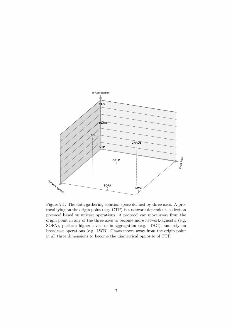
• Network Dependent vs Network Agnostic. Protocols that arehighly network dependent are typically less flexible to network dy-namics because they require topology information to perform point-to-point communication. In contrast, topology agnostic protocols usuallyrely on simpler primitives (like flooding) and are thus more resilientto network changes.
• Collection vs In-Aggregation. In-aggregation protocols performsome degree of data fusion on the way to a sink, whereas pure collectionprotocols retrieve each value in a distinct step instead. The inherentdensity of WSNs makes in-aggregation more attractive as it limitsredundant communication.
• Unicast vs Broadcast. Since a wireless transmission is by naturebroadcast, this is determined by the choice and number of nodes thatare allowed to forward a packet. If all nodes receiving a packet areallowed to process and retransmit it, then we define the protocol asbroadcast-based. On the contrary if there is only one, specific desiredrecipient then the protocol is unicast oriented.
According to the above definitions it seems like an obvious choice to movetowards the traits that are more suitable to the nature of WSNs (networkindependent, aggregation at every step, synchronized broadcast). Indeed,making this decision can yield to more flexible and efficient protocols, bothfrom a time and an energy point of view. However, such a choice is notwithout severe drawbacks.
6
In-Aggregation
Network Agnostic
Broa
dcas
t
CTP
TAG
LEACH
ORLP
SD
LWBSOFA
CHAOS
Figure 2.1: The data gathering solution space defined by three axes. A pro-tocol lying on the origin point (e.g. CTP) is a network dependent, collectionprotocol based on unicast operations. A protocol can move away from theorigin point in any of the three axes to become more network-agnostic (e.g.SOFA), perform higher levels of in-aggregation (e.g. TAG), and rely onbroadcast operations (e.g. LWB). Chaos moves away from the origin pointin all three dimensions to become the diametrical opposite of CTP.
7
When protocols do not follow a structured method of collecting informa-tion (for example by not keeping track of each node’s individual contribu-tion to the global knowledge), or when they do not route information alongstrictly defined paths, they also limit the amount of information the sinkgathers. Practically, having less information means that the sink can com-pute fewer kinds of aggregates, and as a consequence a trade-off betweenefficiency and versatility is created. This trade-off can be clearly ob-served if we specify the categories of aggregates a protocol might be requiredto compute.
2.1.2 Types of aggregates
The types of aggregates can be categorized by two factors: i) whether theyare duplicate sensitive and ii) whether they are decomposable. An aggregateof a data set is duplicate sensitive if it changes either when the set isexpanded with values that already exist, or when duplicate values are re-moved from the set. For example consider the data set {1,2,3,3} and theset in which we removed the additional 3, i.e. {1,2,3}. Then the SUM (aduplicate sensitive aggregate) of the first set is 9 while for the second setit has changed to 6. However, the MIN (a duplicate agnostic aggregate) ofboth sets is the same, i.e. 1.
Furthermore, decomposability means that an aggregate of a data set canbe retrieved by successively applying the aggregation operation to a numberof subsets. In other words, an aggregate is decomposable if a divide-and-conquer approach can be applied to compute it. For example, consider againthe set {1,2,3,3} and its subsets {1,2,3}, and {3}. The DISTINCT COUNT, i.e.the number of unique values, is a non-decomposable aggregate (even if it isduplicate agnostic). There are 3 unique elements in the first subset and 1in the second, but these results cannot be combined in a meaningful waythat results in the correct answer (3) for the original set. Non-decomposableaggregates are thus very challenging as they cannot tolerate loss of informa-tion. Examples of non-decomposable and duplicate sensitive aggregates arethe MEDIAN (the value separating the higher half of the set from the lowerhalf) and the MODE (the value which appears more frequently).
It is plain to see that aggregation protocols that do not handle duplicatescannot straightaway retrieve duplicate-agnostic aggregates (this dependsmainly by where they lie on the first two axes), and all1 protocols thatperform some degree of in-aggregation (their position on the third axis) willface difficulties retrieving non-decomposable aggregates.
1To our knowledge the only group of protocols that can handle non-decomposableaggregates are the protocols that rely on digests. A digest is a data structure of boundedsize, that holds an approximation of the statistical distribution of sensor values in thewhole network. Even though these protocols can compute such aggregates, they exhibitlimited accuracy [16].
8
This analysis clarifies the goal of protocol-design for WSN communica-tion. An ideal protocol should require no network information, have themaximum possible degree of in-aggregation and rely on broadcast, all whilebeing capable of computing even the most complex kind of aggregate. Ourresearch revealed that none of the existing approaches exhibit all of thedesired properties or even three of them at the same time.
2.2 Shortest-path routing
Back in the early 2000s, when the research community was given the chal-lenge of aggregating information from a large-scale sensor network, the firstattempt was to use legacy knowledge from wired networks to build routingtopologies. The result of that effort was a large number of energy-efficientMAC and routing protocols whose approach to data aggregation was organ-izing the sensor nodes in various topological structures, in an attempt toroute data along an optimal, minimum-cost path from the source nodes tothe sink.
Typical solutions like TAG [23] or DB-MAC [7] operate on top of tree-based routing protocols, such as CTP [14] or its predecessors [30] whichperform data collection on similar tree graphs. In other solutions a cluster-based pattern of aggregation is elected instead (e.g. LEACH [15]), or achain is constructed, along which aggregation is then performed (e.g. PE-GASIS [22]). In Figure 2.1 we can see where a few examples from thiscategory lie in our solution space. Though they may perform aggregationat a different scope (different frequency of aggregation), they are on top ofthe collection – in-aggregation axis.
In time researchers realized that this approach has an important limit-ation: creating rigid topological structures, where information has to beforwarded on a specific path, on top of an inherently dynamic system im-poses a high cost. Sensor nodes require many mechanisms at the Data Linkand Network Layers to build the underlying topology, and this topology hasto be updated regularly to cope with changes in the network’s composition.Thus, it was made clear that the price of constructing and maintaining suchstructures was too high to pay, and that a different perspective was needed.
Nevertheless, shortest-path routing protocols excel in handling duplicatesand therefore can easily compute duplicate sensitive aggregates. Also, incase of a static network, where there is no need to reconstruct the topologicalstructure, the shortest path approach is most efficient. That is the reasonwhy even recently some researchers have opted for such an approach [27].
9

2.3 Opportunistic and Multi-path routing
After realizing the above issue, many researchers moved away from rigidstructures and based their approaches on opportunistic routing. In brief,with opportunistic routing a packet is allowed to travel along multiple routestowards the sink, making the propagation of sensor readings more resilientto intermediate node failures or topology changes due to mobility.
Protocols that follow this approach, like ORW [12], use dynamic, anycastor multicast communication primitives over a Destination Oriented Direc-ted Acyclic Graph (DODAG) [18]. The routes are generated dynamicallyvia mechanisms that allow nodes to opportunistically select the message’sforwarders. Depending on their forwarder-selection strategy, various solu-tions have been developed. For example ORPL [8] selects as forwarders thenodes that exist on different branches of a tree towards the sink, regard-less of the cost of each branch. Other approaches like ExOR [5] select onlyone forwarder out of those who opportunistically received a packet, whileSOFA [24] relies completely on gossiping and uses the first random neighborthat acknowledges a reception.
In general opportunistic routing improves latency and energy-efficiency asprotocols are more resilient and flexible. However, allowing packets to travelalong multiple routes makes it challenging to deploy traditional aggregationschemes because the occurrence of duplicates is common. The handling ofduplicates is an important issue that can limit the network’s capability tocompute different types of aggregates (as explained in Section 2.1).
The existence of duplicates is the main issue that in-aggregation multipathprotocols try to resolve. Synopsis Diffusion (SD) [25] for example tries toovercome duplicates through the use of synopsis data structures2. Apartfrom synopses, opportunistic routing protocols account for the existence ofduplicates in various other ways (through push-pull operations that conservemass, by collecting information at intermediate steps before aggregatingthem, etc.).
Opportunistic and multipath routing brought an improvement to the per-formance of data aggregation. These approaches moved protocols towardsthe traits we consider suitable to WSNs (c.f. Figure 2.1). However, intheir majority such protocols still require network information (although toa lesser extent than shortest-path protocols), which is costly to gather andupdate. Furthermore, protocols of this category have critical communica-tion operations, in the sense that senders need the direct acknowledgementof the reception of a message by at least one forwarder. In turn, this gener-ates additional network traffic in the form ACK/NACK replies.
2Synopses are structures that hold representative information about a large dataset [13]. Compared to the data sets they represent, synopses are much smaller, havingabstracted the desired insight from the set and placed it in a small digest (e.g., histogram,bit-vectors, sample, etc.).
10

2.4 Synchronized flooding-based protocols
To overcome the issues of opportunistic routing researchers have proposed anew generation of communication primitives that do not require informationfrom the Data Link and Network Layers. These primitives build directly ontop of wireless broadcast and waste no effort in building a topology. Thisgives them an advantage, as eliminating topology construction overheadsenables the creation of extremely fast and energy-efficient dissemination‘waves’. Furthermore, solutions using this paradigm enforce global networksynchronization; a feature that provides useful benefits.
The importance of synchronization in WSNs becomes apparent when weconsider their energy constraint property. As mentioned before, nodes con-serve energy by duty cycling their radios, which unfortunately has the con-sequence of making them sometimes unreachable. It follows that withoutsome form of synchronization communication between two nodes is hindered,as both of them need to be during their radio-ON phase, otherwise one has towait for the other. By providing global synchronization, scheduling rendez-vous points between nodes can be achieved more easily.
Glossy [11], the pioneer of this new generation of primitives, also usessynchronization to provide an efficient solution to the issues related to theunavoidably high degree of medium sharing between nodes. Instead of em-ploying expensive MAC methods, Glossy simply allows collisions to happen.However, by having a very precise level of synchronization among all trans-missions, it manages to generate constructive interference3 as every node isbroadcasting a packet with the exact same contents. Glossy is a one-to-allcommunication primitive; it relies on flooding4 to propagate the data of onenode to the whole network.
Other researchers have further improved Glossy’s one-to-all primitive [31]and eventually used it to create an efficient routing protocol, named the Low-power Wireless Bus (LWB) [10]. LWB is in essence a scheduler of Glossyfloods, and is thus topology agnostic. This makes LWB very efficient com-pared to other routing protocols since it does not expend time and energyto construct routing tables. Despite that advantage, LWB does not performany aggregation; it actually goes back towards an address centric approachof communication, using each flood to collect a single node’s information.Thus, for the purposes of gathering data LWB behaves just as a collectionprotocol (its place on the 3-dimensional solution space can be seen in Fig-ure 2.1), which leaves much space for improvement considering the benefitsof in-aggregation (c.f. Section 1.2).
3Constructive interference is a phenomenon in which two waves (the packets in ourcase) superpose to form a resultant wave of greater amplitude. Obviously to superposeconstructively, waves/packets need to be the same.
4Flooding is a simple routing algorithm in which every incoming packet is sent throughevery outgoing link except the one it arrived on.[28]
11

12
Chapter 3
Chaos: all-to-all dataaggregation
Our solution to the problem of data aggregation is heavily inspired by Chaos.Chaos is a synchronous all-to-all data aggregation protocol, based on flood-ing. Chaos is only capable of computing aggregates that are both duplicate-agnostic and decomposable, but its efficiency at doing that is superior toany other existing method. Chaos bases its operation on two mechanisms:i) leveraging the capture effect [29] through tight synchronization, and ii) acoordinating structure, called the flags-field. We believe that these mech-anisms are the cause of Chaos’ main shortcomings and this thesis proposesways to overcome them.
In this chapter we provide all the necessary insight on the inner workings ofChaos; how it performs aggregation, what are its limitations, how it uses theflags field and the capture effect, and why those two are responsible for theprotocol’s main problems. First, in Section 3.1 we provide the motivationfor using Chaos as the basis for our own solution (Extreme Chaos). InSection 3.2 an in-depth explanation of Chaos is given. The reader familiarwith Chaos can skip this section and move directly to Section 3.3 where wefully analyze the protocol’s flaws.
3.1 On choosing Chaos
At the end of Section 2.1.2 we described the traits that, according to us, anideal aggregation protocol must exhibit. Our research revealed that thereexists one protocol, namely Chaos, that comes closer to this ideal solutionand can serve as a basis on which to build. By relaxing the very strict timesynchronization requirement of Glossy, Chaos performs aggregation whilethe flood is being spread over the network and continues communicationuntil there is only one final aggregate being forwarded. In this way, Chaoschanges the one-to-all broadcast operation to an all-to-all aggregation one.
13

The result is a highly efficient flooding-based protocol that is to our know-ledge the only protocol capable of providing all-to-all data aggregation inher-ently. Chaos’ efficiency outperforms LWB and CTP both in speed (time tocollect the aggregate), and in energy consumption (time the radio is used).Even when it is compared to just the collection of all sensor values (all-to-one communication), Chaos delivers the final aggregate to all network nodesmore quickly.
Although Chaos is a promising primitive and exhibits many of the pro-posed desired properties (broadcast-based, fully in-aggregating, topology-agnostic), but it is also brittle and limited to the simplest data aggregationoperations (MIN, MAX). This thesis aspires, and to a sufficient extent man-ages, to overcome Chaos’ problems and to provide an improved aggregationprotocol.
3.2 Inside Chaos
In order to understand Chaos we must first explain how it coordinates andsynchronizes the sensor nodes. Then we can proceed to describing the ag-gregation process.
3.2.1 Two synchronization layers
Chaos establishes two layers of synchronization across the network. First,nodes have the same, synchronized radio duty-cycles, and therefore allcommunication happens within successive radio-on phases, which we referto as Chaos rounds (see Figure 3.1(a)). During these rounds nodes arerestricted to communication (they only execute Chaos), while any otherfunctionality (e.g. sampling the sensors, communicating with the Applic-ation Layer, or the execution of another protocol) is allowed only betweenrounds, when the radio is turned off.
Within a Chaos round a second layer of synchronization is imposed. Around consists of successive synchronized slots (seen in Figure 3.1(b)), eachslot with two steps: a communication step and a processing step. In thecommunication step a node can either receive or transmit a packet. Duringthe processing step a node performs any operations required to keep trackof the progress of the Chaos round. Also, if the node received a packet inthe communication step, a part of the processing step is used by the nodeto merge the values received with its current data in order to update itsaggregate.
To maintain slot synchronization, the duration of both steps must be thesame for all nodes. The duration of the communication step is determinedby the length of the packet, which is immutable during a Chaos round.The time given to the processing step can be elected before deployment andremains constant during the network’s operation, regardless of the time
14

Chaos Round
Radio inactive
Wakeup Period
(a) Chaos Rounds
Chaos Round
Chaos Slot
Com
mun
icat
ion
Pro
cess
ing
(b) Chaos Slots
Figure 3.1: A breakdown of the Chaos process.
that is actually required for processing. This way Chaos ensures that allnodes proceed to the next slot at most within a few tenths of microsecondsof one another.
3.2.2 The Chaos round
We will now provide a detailed account of how Chaos computes an aggregatewith the help of its two core mechanisms, i.e the flags-field and the capture-effect-based collision resolution. To keep our explanations clear we will usea simple example that shows the progress of a single Chaos round.
Consider a small clique network of three nodes, with each node holdingan initial value. The goal is for all nodes to identify the maximum value inthe network.
Every Chaos packet has a header and the aggregated value. In this ex-ample, we will only focus on the flags field of the header. The flags fieldcontains one bit for every node in the network, bit 0 belonging to node A, bit1 to node B and bit 2 to node C. Upon receiving a packet, a node performsa logical OR operation between the local and received flags (to keep trackof each node’s contribution) and a MAX operation between the aggregatedvalues (to keep track of the aggregate, in our case the maximum). Havingclarified that, we can now explain how Chaos works; the progress of theround can be seen in Figure 3.2.
15

6 6
7
8
7
8
87
8
8
B
C
A
slot 1 slot 2 slot 3 slot 4 slot 5
Initialization Aggregation Termination
slot 0
Figure 3.2: Execution of Chaos in a 3-node clique network. In each sentpacket, the completion of the flags field is indicated on the left, while theaggregated value is seen on the right.
Initialization: At the beginning of a new Chaos round nodes turn on theirradios, setup their flags by setting only the bit associated with their id, andset their local aggregate to be equal to their initial value (for example thevalue given by their sensor). The resulting state of the packets can be seen inslot 0 of Figure 3.2. Following that, all nodes except one go into a waitingstate where they listen to the channel for an incoming packet. That specialnode that performs the first transmission is called the initiator, and, as itsname implies, is responsible for starting the Chaos round.
Aggregation: As soon as nodes receive a Chaos message, (the communica-tion step of the slot is finished), they update their flags field and aggregatedvalues. If the flags change, the nodes broadcast the updated informationimmediately after the end of the processing step. In Figure 3.2, upon re-ceiving the message from A in slot 1, nodes B and C update their flags-fieldso it indicates that they now possess node A’s information. After that, theysimultaneously send their updated messages in slot 2. Chaos’ tight syn-chronization method enables all receivers to transmit their updated packetsat the same time, practically causing synchronized collisions.
The capture effect is then leveraged to decode information from thesecollisions. Known also as the co-channel interference tolerance [20], thecapture effect is the ability that some radios exhibit when a collision occursin the communication medium. This ability enables them to correctly receivea signal from one source, specifically from the one with the strongest signal,and disregard other sources transmitting simultaneously.
There are two conditions for the capture effect to take place: i) thestrongest signal needs to overpower1 the cumulative interference generatedby other transmitters, and ii) it has to arrive before, or at least simultan-
1Commonly the strongest signal needs to overpower others approximately by a factorof 2 but this value varies between radio transceivers.
16

eously with (microseconds accuracy), other signals. Enforcing one sourceto have a higher signal strength is not feasible in most realistic scenarios.Choosing a higher transmit power does not provide any guarantees, as thesignal strength would also depend on the physical structure of the area fromthe transmitter to a receiver. Additionally, unless there are specific reasonsto favor one source over the rest, doing so would create unfairness.
However, Chaos guarantees that the second condition is always met,through the sharp synchronization it enforces between nodes. In this ex-ample, B’s signal is assumed to be stronger than C’s, and hence, node A isable to decode B’s message in slot 2. Next, node A updates its values andcontinues the aggregation process by sending a message in slot 3.
Termination: Whenever a node receives a message that sets all its flags,it considers the aggregate to be complete and sends a few more messageson the following slots to ensure that all neighboring nodes have the finalinformation. In Figure 3.2, after processing A’s message in slot 3, node Ccompletely sets all the flags. It then stops the aggregation and disseminatesits final information. Note that B does not receive any new informationfrom A in slot 3, thus in the next slot it avoids retransmitting and listensinstead. This behaviour is crucial to the protocol’s efficiency as it favors thepropagation of unknown information in the network, and increases fairnessas all nodes eventually get to propagate their own data. Finally, in slot 4,nodes A and B receive the complete aggregate from C and disseminate theirfinal values in slot 5.
Synchronization: Having clarified the aggregation process we can nowdiscuss how Chaos ensures synchronization. Both slot and round synchron-ization are achieved thanks to one event, which is the transmission of thefirst packet by the initiator. Slot synchronization is quite simple: after thereception of a packet, which ends simultaneously for all nodes, nodes createa highly deterministic timeout to reach the agreed length of the processingstep. When this timeout occurs an interrupt is triggered and nodes transmittheir own data (if there has been an update in the flags). Round synchroniz-ation is more complex and requires: i) the knowledge of the number of slotspassed since the first transmission and ii) the length of a slot. Chaos is ableto acquire this information by timing communication events and using thehop count field of a packet.
17

3.3 Chaos’ problems and limitations
After explaining the inner mechanics of Chaos, we move on to analyzingits limitations in terms of flexibility, scalability, versatility but also speed.Mainly the problems originate from the use of the flags-field.
3.3.1 Scalability
In order to keep track of the nodes’ contributions, the size of the flags mustbe at least n-bits, where n is the number of nodes in the network. This meansthat the space overhead in the packet header is directly proportional to thenetwork size. In practice this causes the scalability of Chaos to be limitedby the maximum possible packet size, 127 bytes for 802.15.4 nodes. Ifwe consider that a few of these bytes are used for some of the protocol’ssecondary mechanisms (synchronization, error-detection), and that anotherpart is reserved for the sensor data (payload), then we see that Chaos isrestricted to networks of less than a thousand nodes.
Moreover, because the flags-field must be transmitted in each Chaos packet,its size also affects the overall latency. The time overhead δ due to the flags-field can be computed as δ = s f/r, where s is the average number of slotsrequired to complete a Chaos aggregate, f is the flags-field size and r is thedata rate of the radio. The number of slots s depends on the network sizeand is approximately 0.7n [19]. Thus, the expected latency overhead dueto the size of the flags-field can be computed as
δ =s f
r=
0.7n2
r. (3.1)
For networks of 100 and 1000 nodes, with a data rate of 250 Kb/s, whichis typical for 802.15.4 devices, the delay imposed by bitmap transmissionswould be 0.028 s and 2.8 s respectively, for each aggregate. Besides latency,there exists a similar overhead for energy consumption because radio trans-missions consume the lion’s share of a node’s battery reserves.
Chaos’ advantage lies on its fast and energy-efficient way of performingaggregation by leveraging tight synchronization and the capture effect. Theconstraints imposed by the flags field (maximum packet size and quadraticoverhead) jeopardize Chaos’ main strength. We argue that to obtain ascalable aggregation mechanism, the governing data structure should berather constant and always fit within the packet constraints of WSNs (datapackets of few tens of bytes).
3.3.2 Resilience to dynamics
Although Chaos is topology agnostic it still requires some network inform-ation in order to operate. Specifically, the network size needs to be known
18

in order to allocate the correct size for the flags field. In case of networkdynamics, which is a common case for WSNs, three problems arise.
First, should additional nodes join the network, there would be no spacein the header to store their contribution to the aggregate and their presencecould not be accounted for.
Second, if even one node leaves the network, others would indefinitelywait for its contribution and never terminate. Even though Chaos imple-ments a timeout mechanism to handle such an event (which could also occurdue to a node failure), nodes will consider their aggregate incomplete (evenif it is correct) and continue communication, wasting energy and time.
Third, even if the flags-field size was able to perfectly adapt to network-size fluctuations, nodes would have to maintain a hash function that uniquelymaps their IDs to each flag. Such a mapping function is called a minimalperfect hash function and requires at least 2.6 bits to represent each ID [2],aggravating even more the scalability problem mentioned in the previoussubsection.
We believe that a flexible and robust aggregation protocol should be tol-erant to some degree of change in the network’s composition.
3.3.3 Efficiency
As we have already mentioned the protocol’s collision resolution relies on thecapture effect combined with a tight synchronization, which allows to cor-rectly decode the strongest of the collided packets. However, achieving theminimum difference in signal strength needed (typically 3dB) for a success-ful decoding is severely affected by the number of concurrent transmitters.Experiments on random topologies have shown that a node receiving pack-ets from just four concurrent transmitters already has a probability of lessthan 50% to successfully resolve the collision [19].
Chaos makes some effort to limit the number of concurrent transmittersby enforcing the flags-field update as a requirement for a node to broadcastits packet. However, this countermeasure is insufficient, as it fails to addressthe following two problems.
First, during the initial slots of a Chaos round there is high chance thatmost nodes will receive new information and thus retransmit en masse inthe next round. These initial ‘broadcast storms’ make it more difficult forthe capture effect to take place especially in dense deployments, which arecommon in WSNs. Figure 3.3 shows this phenomenon in a network of 90nodes. We can see that between slots 5 and 20, there are slots where anhigh number of nodes try to transmit, increasing the risk for communicationfailures. Although we cannot directly see these failures, we can infer themfrom Figure 3.3, through the following observation: right after slots wherea ”transmit spike” occurs we see that the number of nodes that received nopacket increases. This phenomenon is not only the result of the lack of traffic
19

Figure 3.3: Activity over time during a representative round of Chaos, wherewe can observe ’transmit spikes’ in the initial rounds. Timeout means a nodetransmitted a packet on its own to re-initiate the propagation. Rx nonemeans a node received no packet. Rx no delta means a node received butlearned nothing new. Rx delta means a node received and learned somethingnew. Tx means a node sent a packet. (excerpt from Chaos: Versatile andEfficient All-to-All Data Sharing and In-Network Processing at Scale, O.Landsiedel et al [19]).
in the vicinity of those nodes’ transceiver, but its cause can also be that thecapture effect could not successfully resolve the packet. This claim can befurther supported if we consider that the number of nodes not participatingin any communication should not increase so early in the round, as it isvery probable that there is still a lot of new information to be propagatedbetween nodes. In Figure 3.3 nodes that don’t report any communicationhappening (”Rx none”) do not include neither transmitting nodes (”Tx”),nor nodes that received the same information (”Rx no delta”), but theirnumber fluctuates a lot even in the early slots of the round.
Obviously failures in communication slow down the computation of theaggregate, as an unresolved collision practically results in a wasted slot forthe receiver, and possibly for the transmitter too if no other node successfullyreceives its packet. Even worse, collisions could lead to an abrupt radiosilence in case all receivers either fail to decode a packet, or do not get aninformation update. Experiments have shown that this is a quite commonscenario in the first slots of a Chaos round, especially in one hop and cliquenetworks. In networks with such topologies, all nodes but the initiator
20

transmit during the second slot, and it is up to the initiator (who is theonly receiver) to continue the aggregation process. The initiator has tosuccessfully decode a packet from the superposed transmissions of everyother nodes in the network. As one would expect, this often fails and thenetwork then falls in radio silence. Chaos can recover from such a situation,but at the cost of a few slots (typically 3 to 5, as seen in the Timeout ’lines’in Figure 3.3).
Second, in static networks the capture effect will very likely occur amongthe same set of nodes, giving consistent advantage to the strongest nodesirrespective of the contribution their values bring to the aggregate. In casethe most valuable information (e.g. the extreme value) is stored in nodeswith a weak signal, the latency of the aggregation process can be affectedsignificantly.
3.3.4 Aggregate type limitations
The flags field gives knowledge of how many and which nodes contributedto the aggregate, but unfortunately it does not provide information on howevery node has contributed to the (partial) aggregate. The end result of theaggregation process (final aggregate and flags-field) cannot indicate the ini-tial values of each node. Thus, even though Chaos capabilities of computingsimple aggregates (MAX, MIN) are exceptional, they also end there.
Aggregates that requires mass-conservation (e.g. SUM, AVERAGE) and non-decomposable ones (e.g. MODE, MEDIAN) cannot be directly computed by theChaos primitive, as the same values can be retransmitted an undeterminedamount of times, and the knowledge of the initial value of every individualnode is lost during the round. To really overcome this limitation, complexmethods to disaggregate information such as network coding would be re-quired. Ideally, we would like to maintain Chaos’ simplicity while extendingits capabilities to target a wide range of applications.
21

22
Chapter 4
Extreme Chaos
Considering the limitations of Chaos presented in the previous section, wepropose a different aggregation primitive that we dub Extreme Chaos. Ex-treme Chaos is efficient, because it builds upon Chaos’ principles of tightsynchronization, capture effect leveraging and maximal in-aggregation; scal-able, since its overhead scales logarithmically with the network size; flexible,because but it can tolerate nodes joining and leaving the network; versatile,as it is capable of estimating duplicate sensitive aggregates.
The purpose of this chapter is to fully describe how Extreme Chaos op-erates, and provide the motivating insight and an in-depth analysis for thetwo mechanisms we introduce to Chaos. The first mechanism, the estim-ation vector, mainly aims to replace the flags-field, but is also used in theestimation of complex aggregates. The purpose of the second mechanism,the flow control policy, is to limit the number of concurrent transmitters,and increase the chances of obtaining an adequate signal-strength differencebetween received packets; enough for the capture effect to succeed.
First, we analyze those two mechanisms, starting with the estimationvector in Section 4.1. In Section 4.2 we provide details on the workingsof our flow control policy. Having established how these two mechanismsoperate, we describe, in Section 4.3, the aggregation process of our protocolthrough the help of an example, analyzing the transmission and terminationpolicies. Finally in Section 4.4, we explain how Extreme Chaos is capableof estimating complex aggregates.
4.1 Estimation vector
Our analysis of the flaws of Chaos (in Section 3.3) indicates that in order toachieve any significant improvement the flags-field mechanism needs to bereplaced as it appears to be responsible for most of Chaos’ shortcomings. Inits place, we use the estimation vector as the new co-ordinating structurearound which we built the main policies of Extreme Chaos. Like the flags
23

field, the estimation vector is fully decentralized, and moreover it has theadvantages of scaling much better against an increase in network size, ofbeing flexible to a certain degree of nodes joining/leaving the network, andof being ID-agnostic.
The estimation vector is the tool for identifying the network’s contribu-tion to the aggregate and, as will be explained in Section 4.4, for enablingthe retrieval of more advanced aggregates. Therefore, it would not be anoverstatement to say that it is the primary element of our protocol, andunderstanding it is a prerequisite to perceiving Extreme Chaos’ potentialand limitations. In the following subsections we present the rationale forthe estimation vector, and give its implementation details.
4.1.1 Replacing the flags-field
The underlying purpose of the flags-field is not just to provide knowledge ofthe network’s contribution to the aggregate, but to do so in an absolutelyprecise way: by counting. In other words, using flags as a completion metricguarantees that every single node has been polled, and its knowledge ofthe correct aggregate has been accounted for.
We argue that such a requirement is excessively conservative for the follow-ing reason. Naturally, we require a reliable method to compute aggregatesbut we should keep in mind that our (primary) goal is to retrieve simple,duplicate-insensitive aggregates, i.e. the MIN and the MAX. In practice, theextreme values spread quickly over the network, and the majority of nodeshas retrieved them without having to individually inquire every other nodein the network.
One first, naive approach could be to relax Chaos’ termination conditionof totally completing the flags-field, to requiring that only a percentage ofall the flags has to be set. This would provide the protocol with someflexibility to nodes failing or leaving the network, but it would not resolvethe problems related to scalability and ID mapping. Therefore, we opted touse a different structure (the estimation vector) that contrary to the flags-field does not actively count the number of contributing nodes but ratherestimates it. Specifically, nodes try to estimate the network’s size andthen, by comparing it to their knowledge of the actual network size theycan infer the contribution ratio (the closer the estimation is to the networksize, the higher the contribution). Similarly to Chaos, nodes transmit andupdate their estimation of the network’s contribution (the vector instead ofthe flags) along with their aggregate.
4.1.2 A vector of size estimators
Our estimation method relies on order statistics and the propagation ofminimum values (a notion well explored in WSNs [4]). To clarify its oper-
24
ation, we first give a brief explanation of the 1st-order statistic cardinalityestimator.
Given a range of [1-m], the more uniformly random values taken fromthat range, the higher the likelihood of obtaining a minimum with a smallervalue. This trend is known to lead to the following cardinality estimator [6]:n ≈ m/min(r1 . . . rn) − 1, where (r1 . . . rn) are the n random values takenfrom the range [1-m].
An important factor for an accurate estimation of n is to get the ’right’min(r1 . . . rn), i.e. the expected one. This is not always guaranteed becausechoosing the random numbers that form the set from which the minimumis derived is a stochastic process, and, as a result, the minimum will notalways have the expected value.
Thus, the generation of the random values must be repeated several timesin order to produce an accurate estimation. More specifically, multiple setsof random values must be created, and then the minimums of these sets haveto be averaged. The number, k, which we choose to repeat this process, isan important factor that determines the accuracy of our estimation (c.f.Section 5.2).
Our estimation vector, uses the above insights and enables nodes to ex-change many (k) sets of random numbers in parallel, by reserving space inthe packet header for every single one of the k minimums to be found. Inthis way, nodes have k minimums at their disposal to average at the end ofa single Extreme Chaos round. This vector is used by the network nodes inthe following manner:
The estimation vector is initially composed of k integer values, each valuechosen uniformly at random in the range [1,m]. As we mentioned, uponreceiving a message nodes update their vector. The update procedure iseasy as nodes only need to keep track of the minimum value for each ofthe vector’s elements. In other words, they simply perform an element-wiseminimum operation between their local vector (L) and the one they justreceived (R):
Li = min(Li,Ri) , i = 1 . . . k. (4.1)
In doing so, nodes are retrieving the minimums from an increasing poolof random values per element of the vector. It should be noted again thatthe average of these minimums will eventually provide an approximation ofhow many random values are being considered. The maximum possiblenumber of values that can be considered (per element of the vector) is equalto the number of nodes in the network. Therefore, as the round progresses(and the values of more nodes are accounted for) the estimation convergestowards the network size.
After every communication step the resulting vector can be used to updatethe estimation of the network size n based on this equation:
25

n =mk∑ki=1 Li
− 1. (4.2)
which is practically a size1 estimator based on 1st-order statistics, usingthe average of k minimums.
Having acquired n from eq. 4.2 it is only a matter of dividing it with thetrue network size n in order to obtain the contribution ratio cr:
cr =n
n. (4.3)
The accuracy with which we can estimate the contribution ratio is ofutmost importance, something that will be made clear in Section 4.3.1.So far we have suggested that this accuracy mainly comes from the number,k, of parallel experiments we perform, i.e. the size of the vector. Althoughit is not very obvious, the accuracy also depends on the upper bound of therange, m, the choice of which practically limits the maximum network sizewe can estimate. For example if m is 10, then the maximum network sizethe estimator is able to compute is 9 if (at least) one node picks the lowerbound of the range, i.e. 1, as its random value for every element of thevector.
However, increasing either the size of the vector or the available range(the number of bits used to represent each random value) directly leadsto an increased space overhead required to store the estimator. Thus inprinciple, it is important to calibrate k and m in such a way that allowsa good, but not too costly estimation of n. We analyze this trade-off inSection 5.2.
4.2 Flow control
In order to enhance performance, we need to create a mechanism that ad-dresses the capture effect related problems of Chaos. Similar to Chaos, ourpropagation policy suppresses unnecessary transmissions while allowing newinformation to propagate in the network, since it only allows a node to trans-mit on the reception of a different estimation. However, this also causes ourprotocol to exhibit very similar transmission patterns as those of Chaos, andthus, suffer from the existence of too many concurrent transmitters in theearly slots of a round. An example of this transmission pattern on a networkof 16 nodes can be seen in Figure 4.1(a).
As a countermeasure, we employ a flow control mechanism that is pree-mptive, i.e. it tries to prevent congestion from ever happening. It achieves
1The cardinality estimator is ”renamed” to size estimator since now every node gathersvalues from all nodes in the network including itself.
26

that by forcing nodes to have a probability to ”back-off” from a sched-uled broadcast. During the first slots, where a burst of transmissions isexpected, nodes will probabilistically decide to abstain from their scheduledbroadcast operation. The probability with which a node backs off froma scheduled transmission has an initial value that gradually decreases, asbroadcast storms are less frequent and less intense in the later slots. Thebenefit of this policy is that the network suffers from less communicationfailures and thus aggregates values more quickly. In Figure 4.1(b) we can seehow the transmission pattern was smoothed, allowing more nodes to com-plete the round sooner (radio silence, which implies the round’s completion,was achieved in 33 instead of 39 slots). As desired, the policy only changedthe transmission pattern at the beginning of the round.
4.2.1 Exponentially decaying ”back-off” probability
We will now proceed to explain how the value of the the ”back-off” prob-ability, P , of our flow control policy decreases exponentially as the roundprogresses. The reason it follows such a curve is due to the transmissionpatterns a round in (Extreme) Chaos exhibits.
The probability is computed as:
P =
{P0 (q − pr)γ/qγ 0 ≤ pr ≤ q0 otherwise
(4.4)
where P0 is the initial probability, pr is the node’s progress metric, q isa factor that limits the duration of our policy, and γ is a parameter thataffects the probability’s decay rate for the chosen duration.
Tuning these parameters correctly is essential for the effectiveness of theflow control mechanism. Otherwise, our mechanism could have sub-optimalor even negative effects on the protocol’s performance. If the resulting prob-ability from the above equation is too low, then we would not be applyingenough flow control and the capture effect would still have high chances offailure. On the opposite, if the probability is too high and it is applied toofar into the round, we might end up preventing useful transmissions andslow down the aggregate-computation process.
In practice we need to strive for maintaining: i) that the duration of thispolicy is limited, and ii) that the number of nodes to ”back-off” from atransmission is not too high. The first is governed by the parameters q andpr, while the second is governed by P0 and γ.
Although the ’broadcast-storm’ phenomenon appears to have a longerduration on a larger network, we argue that this occurs mainly due to thefact that nodes further from the initiator join the round at later slots. Oth-erwise, the values of nodes converge within their neighborhood relativelyquickly. Therefore, we choose a notion of progress that has a local scope;
27

0 10 20 30 40 50Slot Number
0
1
2
3
4
5
6
7
8
9
10Co
ncurrent Tran
smitters
Flow Control Disabled
(a) Flow control disabled (100% chance to transmit on information update).
0 10 20 30 40 50Slot Number
0
1
2
3
4
5
6
7
8
9
10
Concurrent Tr
ansm
itters
Self Tuned Initial Transmit Probablity
(b) Flow control enabled. The initial probability was determined by the network nodesaccording to their local density.
Figure 4.1: Typical transmission patterns for a network of 16 nodes (numberof concurrent transmitters) with and without our flow control policy. Whenflow control is enabled the maximum number of concurrent transmitters islimited. Although a difference of 2 (from 8 to 6 concurrent transmitters)may not seem significant, if we take into account the size of the networkthis results in a decrease of 12% in the number of concurrent transmitters.This considerably improves the chances of the capture effect succeeding. Inlarger (and denser) networks we expect the effect of flow control to be moreprevalent.
28

specifically we elect pr to be the sum of the number of slots a node hastransmitted, plus the number of slots it should have transmitted but ab-stained (due to the flow control mechanism). To increase fairness we givemore weight to the slots where a ”back-off” happened, so that nodes thatskip their transmission slot more often, have a higher probability to transmitin the future. Therefore pr is given by:
pr = (Stx + 2Sbo)/3. (4.5)
where Stx and Sbo are the number of slots the node transmitted and thenumber of slots it abstained from transmitting, respectively.
We specify that the duration that our flow control policy is in effect,cannot be longer than 20 progress steps, thus q is set to 20. This numberis not chosen arbitrarily; it allows the policy to last for 20 progress steps,i.e. from 30 slots if a node keeps backing off to 60 if a node never backs-off. This is enough for a local neighborhood to stabilize even for densenetworks. It is important to emphasize that the value of q is not meant tobe the determining factor for the value of the ”back-off” probability usedby the nodes. Actually, the probability usually decays to very low valuesbefore 20 progress steps have passed (depending on P0 and γ). Thus, themain purpose of this parameter is to ensure that the flow control policy isdisabled at later slots, acting as a fail-safe mechanism against the rare caseof a node constantly ”backing-off”.
The logarithmic curve, which the ”back-off” probability follows, should berelatively steep because the nodes’ values within a neighborhood convergequite quickly. This steepness is controlled through the parameter γ, whichhas to ensure that the ”back-off” probability does not decay too fast (beforethe neighborhood has converged), or too slow (when new information is notreceived often). After performing experiments with various values for γ (inthe range [0.1, 5]) on topologies of different density and size, we establishedthat a value of ≈ 3.0 provides a suitably steep curve for most networks2.
Finally, the initial probability, P0, has to be decided. Unfortunately,and in contrast to the other parameters, there is no way of correctly choosingits value unless we possess some knowledge of the network and thus, itcannot be a fixed value. To be exact, we need to know the network’sdensity, as this tells us how difficult it would be for the capture effect tosucceed if all nodes in a neighborhood decide to transmit in the same slot.The value of P0 should reflect that knowledge since initially we do expectall nodes in a neighborhood to transmit concurrently. Fortunately, ExtremeChaos is capable of computing a suitable value for P0 for every node in thenetwork.
2According to the results from all the topologies we tested, we suggest that γ shoulddefinitely be larger than 1, which leads to a linear curve, and less than 4, above which theflow control is not in effect long enough to provide any benefits.
29

4.2.2 Self-tuned initial probability P0
For homogeneous networks, where density is similar everywhere, a globalinitial probability can be chosen and set before deployment. However, con-sidering the dynamics inherent to WSNs, such a solution is not realisticallypossible. Thus, we developed a self-tuning mechanism that works togetherwith the flow control policy, and allows nodes to decide on their value of P0
among themselves.
Nodes gather information about their neighbors, specifically their numberand the signal strength of the link they share. As it happens, Extreme Chaos(and Chaos) is quite good at collecting such information, discovering about80% of the existing neighbors within just a single round, as we observed in allthe experiments we performed. The ability to retrieve the local density existswithout interfering with the aggregation process and demands only a smalloverhead (an extra field in the packet header which holds the transmitter’sID).
Having collected this information, nodes can evaluate how difficult it willbe to correctly decode a packet in case of all of their neighbors transmitin the same slot. The result depends both on the number of individualneighbors, and on the number of neighbor pairs with similar signalstrengths. The reasoning behind this is that the capture effect will succeedwhen there is a significant difference3 between the stronger signal and therest. Thus the value P0 is given by:
P0 = min(0.9, 0.1(c+ p)) (4.6)
where c is a node’s cardinality, and p is the number of pairs of networknodes with a signal strength difference of less than 3dB.
Nodes broadcast their own calculated P0 in every round and they alsokeep track of the maximum P0 received. The maximum of the receivedP0, reflects the highest density among every node’s neighbors. Then, in thefollowing round, nodes use this maximum as their own initial probability forthe flow control mechanism, in order to enable even the neighbors with thehighest density to reliably decode a packet. By continuously re-evaluatingP0, our technique adapts to network dynamics.
Finally, we should mention that there are two exceptions to this policy.Obviously, the initiator must always transmit on the first slot. Apart fromthat, nodes with just one neighbor are also exempted as they might be vitalto the network’s connectivity, and because they do not get many opportun-ities to propagate their information (they have only one potential receiver).
3In the CC2240 RF transceiver used in our experiments the capture effect in known tosucceed reliably when the signal-strength difference is 3dB.
30

A
B
C
slot 0 slot 1 slot 2 slot 3 slot 4 slot 5
Initialization Aggregation Termination
7 3 9 53% 6
9 8 4 48% 7
5 2 6 77% 8 5 2 6 77
% 8
7 3 9 53% 6 5 2 6 77
% 8
5 2 4 91% 8
5 2 4 91% 8
5 2 4 91% 8
Figure 4.2: Execution of Extreme Chaos in a 3-node clique network. Anestimation vector with k = 3 and m = 10 is used. In each sent packet, firstthe 3 elements of the estimation vector are shown on the left. Then, theresulting contribution ratio (rounded to the closest integer) is shown in themiddle, and last the aggregated value in indicated on the right.
4.3 Inside Extreme Chaos
After giving an overview of the new elements introduced (estimator, flowcontrol), we proceed to explain in detail how our core mechanisms are usedby revisiting the 3-node example of the previous chapter. Extreme Chaosfollows the same three operating phases as Chaos but with some key differ-ences. Synchronization on the other hand is achieved identically as in Chaoswith the same two layers of synchronization (rounds and slots).
4.3.1 Initialization
At first nodes generate random values in order to setup their estimationvector. From this vector, the network size and thus the contribution to theaggregate can be derived. In slot 0 of Figure 4.2, we can observe how closethe initial estimation is to the actual network size. At first, it might varya lot between nodes, the reason being that our estimator is essentially aprobabilistic technique. However, as nodes transmit and update the estim-ation vector, their estimations converge to the same value (approximatelythe actual network size). Like in Chaos, the initiator starts the round (slot1) by making the first broadcast, the event around which all other nodes inthe network synchronize.
4.3.2 Aggregation
Similar to Chaos, our mechanism monitors the number of contributing nodesin order to decide if the aggregate is complete. Upon receiving a message,nodes aggregate the information, and update their estimation vector and/orthe aggregated value, according to the message’s contents. Unlike Chaos
31

however, nodes do not necessarily retransmit their packets when the estim-ation vector is updated. Whether they actually do also depends on the flowcontrol mechanism.
Although the network in this example is too small (and sparse) for any flowcontrol to be really needed (something our mechanism normally recognizes),we illustrate what is likely to happen on larger networks in slots 1-2 of thisexample. Even though both Nodes B and C updated their estimation andtheir aggregate in slot 1, only C transmits in slot 2 as B was prevented todo so by the flow control mechanism.
This behaviour is beneficial to the protocol: the existence of fewer con-current transmitters means that the capture effect has more chances of suc-ceeding (in this example the capture effect is not needed at all as there isonly one transmitter). Moreover, the node that abstained from transmittingis not really penalized as it still gets to gather new information. Finally, oneless obvious advantage is that this method is more fair to nodes with weaksignal strengths. In the case of Chaos, Node B, which we assume to havea strong signal, will always be the one to get its packet decoded in slot 2.However, our mechanism allows Node C to sometimes get its informationthrough first. In denser topologies, the benefits of the flow control mechan-ism are more prevalent (the probability of the capture effect succeeding isaffected more drastically).
Aggregation continues in slot 3. In this example Node B again ”backs-off”from transmitting in this slot. Node A has updated its estimation vectorand its aggregated value, and is the only transmitter.
4.3.3 Termination
To deem the aggregation process complete Extreme Chaos requires that theestimated contribution, i.e. how close the estimated size is to the actual net-work size, has reached a certain threshold. Once this threshold is crossed,the contribution ratio is considered to be high enough to assume the aggreg-ate held by a node to be correct. The intuition behind this notion is simple:the progress of the size estimator (the MIN of a set of values), precisely fol-lows the propagation of the aggregated value over the network (because italso is a MIN or a MAX). An adequate contribution ratio implies that theextreme value we are trying to retrieve is held by all network nodes withhigh probability, and thus nodes can be allowed to terminate the round. Wecall this termination policy the contribution criterion. In Figure 4.2 nodeB crosses the specified threshold (80% for reasons explained below) in slot4 and then the network enters a dissemination phase similar to the one ofChaos.
The value of the threshold is vital to the contribution criterion and mustbe chosen carefully. This choice is bounded between two values. The lowerbound depends on the propagation speed of extreme values. For example, if
32

we know that in the topologies we target, a maximum has assuredly propag-ated over the network when the contribution is at 60%, then that shouldbe the lower bound for the threshold’s value. An even lower value wouldmake some nodes to terminate the round prematurely, before finding themaximum.
The upper bound is restricted by the accuracy of our size estimationtechnique. Our estimator computes a value that is usually either larger,or smaller than the real size, and the variance depends on its accuracy.The upper bound has to respect this limitation. For example if we knowthat we can estimate the network size with at most 60% accuracy, settinga threshold of 70% would mean that when the size is underestimated bymore than 30% the contribution criterion is never satisfied and the roundcan not finish. Given our tested parameters, our size estimation techniqueprovides accuracy of more than 80% (see also Section 5.2). This accuracy isgenerally enough to ensure that the extreme values have propagated globallyeven when they were held by nodes at the edge of the network.
Practically, we elect the threshold’s value to be equal to the upperbound because the value of the lower bound depends on many factors wecannot control (topology, location of the extreme value, etc.).
However, when the network size is overestimated our estimator mightstill violate the lower bound. This is better explained with the help of anexample. If we trust that the accuracy of our estimator is 80%, then thismeans that on a worst case overestimation, the estimator will be progressingtowards a network size that is 120% of the actual one. Based on our explan-ations for choosing the threshold, in a network of 100 nodes we would allownodes to terminate only if they are estimating a size of at least 80 nodes(which is the upper bound). However, in our example nodes falsely thinkthey reside in a network of 120 nodes (because they are overestimating). Asa result, the estimated size will advance more quickly than normally andits value will reach the critical mark of 80 nodes, approximately when just80%/120% = 66% of the network has been covered, which is not alwaysenough to reliably retrieve the extreme value.
To compensate for the above shortcoming of our estimator, we imposeda secondary condition, the steady-state criterion. The steady-state criterionworks when Extreme Chaos has reached the termination phase, i.e. whenthe contribution criterion has been satisfied. Under normal circumstancesnodes in the termination phase disseminate their information a small num-ber of times and finish the round. We call this number the protocol’s stabilityfactor and a stability counter exists to notify the node that the necessaryamount of disseminating transmissions has been reached. The steady-statecriterion dictates that if a new aggregate arrives during this phase the stabil-ity counter resets, allowing more time for the network to properly converge.Through this countermeasure we increase the robustness of the protocolagainst premature termination.
33

4.4 Complex aggregates
Attempting to expand Chaos’ capabilities to a larger set of retrievable ag-gregates proved to be a real challenge. To our knowledge it is impossibleto keep track of duplicates without either resorting to methods that workon top of rigid structures, or reverting back to collection schemes. How-ever, there still exists a chance to increase our protocol’s versatility in usinggossiping techniques capable of estimating complex aggregates. Such tech-niques can fit naturally within the capabilities of our protocol and leave thetopology-agnostic aggregation process undisturbed.
The core mechanism of Extreme Chaos, i.e. the estimation vector, is sucha technique. Thus, more than just defining the termination policy, it canbe used to expand our protocol’s capabilities further than its predecessor.In fact we have already given the protocol this capability by estimating theCOUNT of the nodes existing in the network, i.e. the network size, which weuse to determine the contribution ratio.
One could argue that Chaos is also capable of computing COUNT aggregatesand in a more deterministic way than Extreme Chaos; the flags field ispractically a way of counting nodes in the network. While this is true, thereis a significant difference: chaos uses the result of the COUNT for making itsmechanism work, while Extreme Chaos does not. Though both protocolsmake use of the network size in their mechanisms, Extreme Chaos simplyrequires it to compute the contribution ratio, while Chaos needs it to knowexactly how many bits to allocate for the flags-field.
For both protocols though, the procedure of counting something otherthan the network size (for example how many nodes hold a particular prop-erty) is similar. The coordinating structure needs to be duplicated, ini-tialized in a different way, and then transmitted and updated normallyalong the original one. The advantage we have over Chaos is in terms ofscalability and flexibility. Not only does our estimator requires a much smal-ler space overhead (c.f. Section 5.2), but it also does not require a-prioriknowledge of the value we are trying to estimate (or an upper bound to it).Additionally, this allows us to estimate aggregates such as SUM and AVERAGE,something Chaos cannot do.
We now proceed to explain how the duplicated vector needs to be initial-ized for the cases of COUNT and SUM.
While estimating the COUNT of nodes with a certain property, nodes notexhibiting that particular property must make sure that their vectors willnot affect the estimation process. Therefore, they have to initialize everyelement of their vector with the maximum possible value, i.e. m, instead ofusing random values. This has the same result as creating fewer vectors: tobe precise it is the same as generating COUNT vectors. Computing the SUM isless obvious and requires a brief explanation.
34

The solution again resides in proper initialization of the secondary estim-ation vector. To sum, each node initially computes x estimation vectors,where x is the value the node wants to contribute to the SUM. Before start-ing the aggregation phase, the node computes the element-wise minimumbetween the elements of the x vectors (Equation 4.1), and stores the resultsas its initial (secondary) estimation vector. Then, the mechanism proceedsas normal.
An easy way to intuitively understand why the above leads to a correctresult is to consider the following. When we use estimator vectors to measurethe network’s size a number of vectors equal to that size is generated. Byletting nodes generate more vectors and ’internally’ retrieve their point-wiseminimum practically we simulate the existence of more nodes in the network.Therefore we estimate the SUM of all values held by the nodes, by estimatingthe size of a virtual, larger, network.
With SUM and COUNT, Extreme Chaos can also provide other estimationslike AVERAGE.
35

36

Chapter 5
Evaluation
So far we have claimed that we created a protocol that is more efficient,flexible, scalable, and versatile than its predecessor. In this chapter, weprove that Extreme Chaos does indeed possess the above qualities. First, inSection 5.1, we give an overview of the configurations in which our protocolwas deployed, and the evaluation metrics we used. Then, in Section 5.2, webegin our evaluation, by providing a scalability analysis of our estimator interms of space overhead. In Section 5.3, we assert the protocol’s performancein finding correct duplicate-agnostic aggregates, in a short amount of time.Section 5.4 examines Extreme Chaos’ tolerance to network changes. Finally,Section 5.5 shows the achievable accuracy for more complex aggregates,taking the SUM as a case study.
5.1 Testbeds and Evaluation Metrics
In order to evaluate Extreme Chaos, we implemented our protocol on TelosBnodes with Contiki OS. We then ran an exhaustive set of experiments on twodifferent testbeds: Flocklab[21], and a local testbed, consisting of 9 nodesconfigured in a clique network. To prove specific points, we occasionally ransimulations either in the Cooja simulator, or in Python.
Table 5.1 summarizes the experimental setup. Note that both testbeds aredeployed in an office environment and were operated both during working,and night hours, in order to ensure that the aggregation mechanisms weresubject to all kinds of environmental conditions.
Although we tested several topology scenarios to reveal all the minoraspects of our protocol, all our experiments used a constant slot lengthof 14ms (4 ms for packet transmission and 10 ms for packet processing).Where applicable we compared our Extreme Chaos to Chaos. Finally, resultspresented are averaged over approximately 500 aggregation rounds.
37

Flocklab Local
Size(s) 16-24 9Tx Power [dBm] 0 0Diameter 4 1Initiator ID 022 1Node degree 8.5 8
Table 5.1: Testbeds’ characteristics and experiment setup.
We evaluated the performance of our aggregation protocol using the fol-lowing four metrics:
Convergence Time. This metric is defined as the average time needed tocomplete a successful all-to-all aggregation, starting when a node enters anaggregation round, and ending when it stops its termination phase. Notethat this metric accounts also for the rounds in which the aggregation fails(e.g. because the completion conditions are not met). In this case the roundends when a guard timeout triggers (in our experiments, 1700 ms).
Coverage. This metric indicates the average of the true contribution ratioperceived by each node at the end of aggregation. In other words, it showsthe average percentage of nodes whose values have been considered in orderto compute the round’s aggregate.
Success Ratio. The success ratio indicates the average fraction of nodesthat successfully compute the correct aggregate at the end of each round.
Relative Error. This metric measures the estimation error averaged overseveral aggregation rounds. The relative error is computed as |a − a|/a,where a is the correct value and a is its estimation.
5.2 Scalability
Before evaluating the scalability of Extreme Chaos, it is vital to explain howto decide on the two parameters that characterize its estimation mechanism:the size of the estimation vector (k), and the maximum value the randomnumbers can take (m). In particular, we want to point out the relationbetween the estimation error, and the overhead that incurs when using largerk and m.
Because the size estimator in Eq. 4.2 is independent of the underlyingcommunication phenomena, the results proposed in this section are gener-ated from Monte Carlo simulations running in Python.
38

Figure 5.1 shows the effect of different k and m in a 40-node network andleads to the following two observations:
First, increasing the number of parallel experiments (i.e. the vector sizek) provides an improvement that is, initially, significant but decreases quitedrastically. The results suggest that a value of 25 experiments provides agood trade-off between low estimation errors (always ≤ 0.2) and low spaceoverhead (25 log2(m) bits).
Second, changing the range m does not seem to affect the estimation error.However, we expected that as m decreases, so would the accuracy. Thereason is that our estimator receives its accuracy mainly by averaging outk observations (a minimum per element of the vector). Some observationsare higher, and others lower than the expected value (which would providea correct estimation). As the network size approaches m, we expected ourestimator to provide increasingly lower estimations because the availableprecision bounds the lower value (it cannot be less than 1) of an observation. Thus, the average observation is biased towards a value that is higherthan the expected one, something that should lead to a smaller estimatedsize. However, in our case, even with the narrowest range tested (m = 28 =255), the network size is far smaller than the one needed to test the abovehypothesis.
To better understand the relation between the range m and the networksize n, we ran our estimator on a wide set of network sizes, which rangedfrom 10 to 10,000 (the parameter k was fixed to 25). The results, depictedin Figure 5.2, show that indeed the estimation error starts growing as thenetwork size n gets closer to the range m. Therefore, by setting a conser-vative range for m to 2-4 times the network size n, we are able to providelow estimation errors (≤ 0.2), while keeping an overhead that is logarithmicto the network size.
For example, with conservative values for m = 4n and k = 25, our es-timator shows lower overheads than Chaos’ flags-field for networks that arelarger than 249 nodes (see Figure 5.3). With a less conservative approach(m = 2n and k = 20) we could overcome Chaos’ overhead after 167 nodes.
5.3 Reliability and speed
While scalability is an important characteristic, we still want our mechanismto compute aggregates with speed and accuracy that is comparable, or betterthan the existing mechanisms. To test this, we scheduled several experimentswhere Chaos and Extreme Chaos computed a MAX aggregate.
For Extreme Chaos, we also explored the effects of increasing the numberof slots (1, 3, 5 and 10) nodes need to wait after they satisfy their con-tribution ratio before terminating their aggregation (i.e. different stabilityfactors). We expected that a higher stability factor can make our protocol
39

Parallel Experiments [k]0 10 20 30 40 50 60 70 80
Re
lative
Err
or
0
0.2
0.4
0.6
0.8
k = 25
m = 28
m = 212
m = 216
m = 220
m = 224
m = 228
Figure 5.1: Estimation accuracy for different vector sizes (k) and ranges (m)in a network of 40 nodes.
Network Size [n]10
110
210
310
4
Re
lative
Err
or
0.2
0.4
0.6
0.8
1
m = 28
m = 29
m = 210
m = 211
m = 212
m = 213
m = 4 n
Figure 5.2: Estimation accuracy for different ranges (m) and network sizes(n), and a fixed vector size (k = 25). By setting m = 4n (white circles) theestimation accuracy is always ≥ 0.8.
Netwrok Size [n]0 100 200 300 400 500 600 700 800
Ove
rhea
d [b
yte]
100
101
102
ChaosExtreme Chaos
Figure 5.3: Overhead comparison between Chaos and Extreme Chaos withincreasing network sizes. For Extreme Chaos, k = 25 and m = 4n. WhileChaos scales linearly with the network size, Extreme Chaos scales logarith-mically (Y-axis is in log scale).
40

Time [ms]400 450 500 550 600 650 700 750 800
Su
cce
ss R
atio
0.94
0.96
0.98
1
stab 1
stab 3
stab 5
stab 10
chaos
Extreme Chaos Chaos
(a) Local Testbed.
Time [ms]400 450 500 550 600 650 700 750 800
Su
cce
ss R
atio
0.94
0.96
0.98
1
stab 1
stab 3stab 5
stab 10chaos
Extreme Chaos Chaos
(b) Flocklab.
Figure 5.4: Aggregation accuracy and convergence time of Chaos and Ex-treme Chaos on our Local Testbed and on Flocklab.
more reliable at the cost of speed. We call these versions of Extreme Chaosstab 1, stab 3, stab 5, and stab 10, respectively.
By looking at the Success Ratio and Convergence Time in Figure 5.4, wecan notice that, independently of the network, Extreme Chaos is able tocompute the aggregate with similar accuracy and shorter convergence times(from 10 to 46%).
Even with the smallest stability value (stab 1 ) the aggregation of ExtremeChaos does not terminate too quickly – due to false, temporary steady states– but waits for the contribution ratio to cross a given threshold (0.8 in theseexperiments).
It is interesting to note that although the remote testbed (FlockLab) islarger than the local one, Chaos needs less time to complete aggregation onit. The reason is that the local testbed is a clique network, and often suffersfrom falling into abrupt radio silence on the second slot (see Section 3.3.3).
Effect of flow control policy: The above results show the overall speedupExtreme Chaos achieved, but fail to capture the contribution of our flowcontrol policy. To illustrate the effectiveness of our flow control we madethe following comparison: we measured the speed of our protocol when theflow control mechanism is deactivated, when a global initial probability, P0,is used, and when nodes autonomously decide on the value of P0.
41

n/a 0.1 0.2 0.3 0.4 0.5 0.6 0.7 0.8 self"Back Off" Probability
550
600
650
700
750
800
Conv
erge
nce Time
No Flow ControlGlobal Initial PropabilitySelf-Tuned Initial Propability
(a) Local Testbed.
n/a 0.1 0.2 0.3 0.4 0.5 0.6 0.7 0.8 self"Back Off" Probability
550
600
650
700
750
800
Conv
erge
nce Time
No Flow ControlGlobal Initial PropabilitySelf-Tuned Initial Propability
(b) Flocklab.
Figure 5.5: Convergence time for different P0. The first bar (P0 = n/a)shows the time required when the flow control policy is disabled. The fol-lowing bars, up to P0 = 0.8, show the result of applying an increasing, globalinitial ”back-off” probability. The bar with the red border is the ”oracle”,i.e. the best global initial probability we could have chosen. The last bar(marked as self ) indicates the performance of the flow control policy for anautonomously chosen P0. The convergence times presented for FlockLabresult from a different, more dense, topology than the one used for otherresults.
42

These experiments revealed that increasing the initial ”back-off” probab-ility of the flow control can help performance up to a critical turning point.After that point any further effort to reduce congestion results in a sub-optimal performance or even a degradation. The reason is that if we restricttoo many nodes from transmitting, then we are actually preventing usefultransmissions from occurring, which delays the aggregation process.
We could thus claim that there is an ”optimal” initial probability thatcan be globally applied to all nodes (which we call the ”oracle”). The auto-tuning version of our technique can usually achieve speedups that are slightlysmaller than the oracle. This can be seen in Figure 5.5; the performanceof the self-tuning version is not far from the best global P0 (≈ 0.4 for bothtestbeds).
However, in some topologies, like sparse networks and loosely connectedones, applying a global value for P0 proved harmful to the overall latency.The same held true for non-homogeneous networks, where the distributionof nodes is not uniform, and areas of different density exist. In such cases an’optimal’ global P0 cannot really be defined. These are the types of networkswhere our self-tuning technique outperforms the oracle, because it is able todetect the different local densities and adjust P0 accordingly for every node.As a result, even in such topologies our flow control policy can either limit
n/a 0.1 0.2 0.3 0.4 0.5 0.6 0.7 0.8 self"Back Off" Probability
550
600
650
700
750
800
Conv
erge
nce Time
No Flow ControlGlobal Initial PropabilitySelf-Tuned Initial Propability
Figure 5.6: Flow control in a sparse topology of Flocklab incurs a decrease inperformance. In such sparse networks there are not many concurrent trans-mitters in the first place, and any effort to limit them delays the aggregationprocess. Our self-tuning mechanism detects this and limits the degradationby keeping P0 to low values.
43

the degradation, or even provide a speedup (results from a sparse networkcan be seen in Figure 5.6).
5.4 Flexibility to network dynamics
Nodes may decide to leave the network either voluntarily or due to a systemfailure causing the effective network size to decrease. Our protocol’s flexiblepolicies allow it to tolerate some degree of change, making it more robustagainst node failure, and more suitable for dynamic networks. To evaluatethe degree of flexibility Extreme Chaos possesses, we supplied our protocolwith false information about the actual network size (we reported a largersize to be used for deriving the contribution ratio), and measured the impactthis had on the protocol’s speed.
Figures 5.7(a) and 5.7(b) show that as the difference between the actualsize and the supplied one increases, the amount of time required to completethe protocol increases. To emphasize on the improvement from the previousversion of the protocol, we also show the speed of Chaos, which degradesdrastically even with a single node failing.
For completeness, we also examined the effect of additional nodes joiningthe aggregation process. To compare against Chaos, which normally does
Time [ms]400 600 800 1000 1200 1400 1600 1800 2000
Success R
atio
0.94
0.96
0.98
1
1%10%
25%50% chaos
(a) Local
Time [ms]400 600 800 1000 1200 1400 1600 1800 2000
Success R
atio
0.94
0.96
0.98
1
1%10%
25%50% chaos
(b) FlockLab
Figure 5.7: Effects of different percents of nodes failing (1, 10, 25 and 50%)on the aggregation accuracy and convergence time. For Chaos, we onlyvisualize one point, since the mechanism times out (1700 ms) as soon as onenode fails.
44
not make any provisions for nodes joining, we made the following modific-ation: extra nodes are allowed to choose a random flag in the flags-field.Additionally, in every message there exists a second flags-field based on thetrue network size, i.e. with enough places for every node that joined. Weadded that field to Extreme Chaos as well. We then compared the two pro-tocols on their ability to complete the extra flags structure that accuratelymeasures the achieved network coverage.
The results are shown in Figures 5.8(a) and 5.8(b). Chaos behaves asone would expect. The original flags-field is filled at an increasingly fasterrate as more nodes join the network. As a result, the aggregation protocolfinishes more quickly even though more values need to be aggregated. Ofcourse, this has a serious effect on Chaos’ ability to poll the entire network,which degrades quickly.
One might expect Extreme Chaos to follow a similar pattern but insteadwe see a completely different behavior. At no increase in network size, orfor very small ones (up to 10%) the achieved coverage of Extreme Chaos isstill a bit lower than that of Chaos, something that is expected given thatour protocol is less conservative. The ”relaxed” method for estimating thenetwork’s contribution (estimation vector) allows our protocol to seamlesslyadapt to changes of network size, when the percent of change is withinthe accuracy of our estimator. The convergence time for Extreme Chaos,which remains less than that of Chaos, also proves the previous claim. Inall accounts, Extreme Chaos has retained its capabilities.
Surprisingly, for medium increases (50%) our protocol is still largely un-affected, or performs only slightly worse than before. One might expect abehaviour more similar to Chaos, meaning a decrease in both convergencetime and network coverage. In Chaos such a decrease was explained; theextra nodes fill the original flags-field quickly, forcing a termination of theaggregation process before all sensor values have been considered. On thesame basis the extra nodes should degrade the performance of ExtremeChaos in a similar manner: the estimated size will increase very quickly (weare now estimating a significantly larger network) and the contribution ra-tio will cross the contribution threshold prematurely. However, our secondtermination condition, the steady state condition protects our protocol fromthis problem. Although nodes think they have explored the largest part ofthe network, a steady state for their estimation vector and their aggregateis not reached yet. The reason is that the values of the network nodes havenot yet converged and thus, the aggregation process is maintained alive.
When the joining rate becomes too high (100% extra nodes) the estim-ated size increases to become much larger than the network size known byExtreme Chaos nodes. It actually becomes larger than what the accuracyof our estimation technique should allow. We mentioned in previous Sec-tions that the accuracy of our estimator is a bit higher than 80%. Then,for example, on a network of 100 nodes we should rarely retrieve an estim-
45

Time [ms]400 600 800 1000 1200 1400 1600 1800
Covera
ge
0.7
0.8
0.9
1
10%50%
100%10%
50%
100% Extreme Chaos Chaos
(a) Local
Time [ms]400 600 800 1000 1200 1400 1600 1800
Covera
ge
0.7
0.8
0.9
1
10%50%
100%10% 50%
100%
Extreme Chaos Chaos
(b) FloockLab
Figure 5.8: Effects of different percent of nodes joining the network (10,50 and 100% compared to the original size) on the coverage (network con-tribution) and convergence time. Coverage is indicated by the percent ofcompletion of a second flags-field in the header of Chaos and Extreme Chaos,which has the correct size.
ation that is larger than 120 nodes, and sizes even larger than that shouldnever be estimated. Our protocol identifies these abnormally high estima-tions that occur when too many extra nodes have joined. With that clue itinfers the existence of extra nodes, and then Extreme Chaos relies only onthe steady state condition to decide on the termination of the round, usinga reliably high stability factor (> 10). This allows polling every part of thenetwork (100% success ratio and coverage) at the cost of speed. For thesame case, Chaos terminates aggregation much faster, but at a severe costin its achieved coverage that is also reflected on its reliability (success ratioof 85.5% for the local testbed).
46

Time [ms]400 600 800 1000 1200 1400 1600 1800
Rel
ativ
e Er
ror
0.12
0.13
0.14 stab 3stab 5
stab 10
stab 15
(a) Local
Time [ms]400 600 800 1000 1200 1400 1600 1800
Rel
ativ
e Er
ror
0.12
0.13
0.14
stab 3stab 5
stab 10 stab 15
(b) FlockLab
Figure 5.9: Estimation error for SUM computation in Extreme Chaos.
5.5 Estimation of duplicate sensitive aggregates
Finally, we show how Extreme Chaos is capable of estimating more complexaggregates with the help of our estimator, using the case of the SUM aggregateas an example. In this experiment the nodes try to compute the sum oftheir IDs (1 to n), with n being the network size. Since the accuracy ofour estimator is now of even higher importance (as it directly affects thecorrectness of aggregation), we use a higher k (35) for our SUM estimationvector to achieve the smallest relative error possible.
Also because these types of aggregates need information from all nodes,we experimented with even higher values for the stability factor. Howeverin Figures 5.9(a) and 5.9(b) we observe that investing in more time to letthe network converge does not decrease the relative error significantly; theerror remains bounded by our estimator’s accuracy. The reasons behind thisphenomenon are discussed in Section 6.1.
47

48

Chapter 6
Discussion
We believe our protocol to lie in the same league as the state-of-the-art ofWSN aggregation protocols, however we recognize that it is but a smallstep towards a new generation of network agnostic protocols. There are stillmany directions to be explored and many ideas to be tested. Chaos andExtreme Chaos can not only serve as powerful tools, but also as platformson which new approaches can be experimented with.
In this Chapter we briefly describe two of these approaches and improve-ments we have planned as future work. In Section 6.1 we analyze the conceptof a lightweight version of Chaos, which has no governing organizing struc-ture, but simply relies on the convergence of the values exchanged betweenthe nodes. In Section 6.2 we propose a dynamic channel hopping schemeinspired by our flow control mechanism and recent improvements on theChaos protocol.
6.1 Chaos: A distributed control system?
During our last stage of experiments with Extreme Chaos, where we usedit to estimate the SUM aggregate, we were interested in polling the largestpossible part of the network, so our estimator could achieve a high precision.The reason why we wanted to achieve a network contribution as high aspossible was that now a vast number of random values were generated (twoestimation vectors were filled with a total k of 55) and the minimums to beretrieved were held by many different nodes. The accuracy of the estimatedSUM depends on the ability of our protocol to poll the entire network andgather all minimums.
Our primary solution, in order to enhance our protocol’s network cover-age, was to increase the stability factor (number of rounds after which thesteady state criterion is satisfied). What we noticed was that almost totalnetwork coverage is achieved even with the smallest stability value (98% ofthe network polled with a stability factor of 3). The explanation of why
49
we achieved such high coverage so easily is actually quite simple: the veryexistence of such a multitude of different values (which must converge) is,on its own, sufficient to force the aggregation process to continue becauseit makes the steady state very difficult to be reached.
This in turn led to two realizations: i) the degree of exploration we desirecan be elected by a correct choice for k, and ii) the contribution criterion(requiring that the estimated size has approached the actual, known size)can be obsoleted. The first claim follows directly from the results of the SUM
aggregation experiments (Section 5.5). To explain why our contributioncriterion can be obsoleted we need to elaborate further.
We can perceive Chaos as a distributed control system with a transitivestate, where nodes adjust their outputs based on different input values untilthey all reach a common steady state (same aggregated value). The originalChaos provides a robust transitive state (through the flags field) that enablesall nodes to reach the common steady state, but it achieves this at the cost ofhigh overheads and low flexibility. Our version reduced these overheads. Byrelying on an estimation, Extreme Chaos keeps communication alive untilthe steady state is reached, though not as reliably as Chaos.
However, both mechanisms interfere with the very transition they try tocoordinate. If we allow nodes to only converge on one value (the MIN orMAX), then nodes converge much faster exploring only a small part of thenetwork. Specifically, they explore only the part of the network necessary toretrieve a stable aggregate. The question that arises is whether that stableaggregate is also the correct one.
We have performed some preliminary tests based on the above observa-tion. For our purposes, we used Extreme Chaos while removing the contri-bution condition for our termination policy (k = 0 and no size estimationwas made). With this modification a node quits an aggregation round basedonly on the steady state criterion, i.e. as soon as it receives the same in-formation a number of times equal to the stability factor. As Figures 6.1(a)and 6.1(b) show, this provides a much faster aggregation primitive that,with correct tuning of the stability factor, can also prove to be reliable. Anadditional advantage of this approach is that the protocol becomes trulynetwork agnostic, as the demand of Extreme Chaos for (approximate) know-ledge of the network size is now non-existent. Scalability is also improvedsince practically this is a zero-overhead primitive.
Promising as it may seem, we should note that the low network coverageof this method can lead to failures in finding the correct aggregate. Forexample, if the extreme value is held by a weakly connected node it mightnever be discovered if this node cannot get his data disseminated in time(before the rest of the network stabilizes). Furthermore in our experimentswe conveniently assumed that the nodes’ initial values are unique. For thepurposes of retrieving extreme values this is the same as having a perfectlyuniform distribution of values, something which works in favor of this ap-
50

Time [ms]200 300 400 500 600 700 800 900 1000
Su
cce
ss R
atio
0.94
0.96
0.98
1
stab 1
stab 3
stab 5stab 10
chaos
Extreme Chaos Chaos
(a) Local Testbed.
Time [ms]150 200 250 300 350 400 450 500 550 600 650
Su
cce
ss R
atio
0.7
0.8
0.9
1
stab 1
stab 3
stab 5 stab 10chaos
Extreme Chaos Chaos
(b) Flocklab.
Figure 6.1: Aggregation accuracy and convergence time of Extreme Chaoswith k = 0.
proach as it allows the aggregation process to continue without creating’false’, early steady states.
Ultimately, we hope that through proper calibration of k, m (to valuesmuch smaller than those used by Extreme Chaos’ estimator), and the sta-bility factor we can achieve an aggregation primitive equally reliable andperhaps more efficient than Extreme Chaos. In any case though, we areconfident it will be significantly more scalable and flexible.
6.2 Extreme channel hopping
A recent work on Chaos proposed a multichannel approach to the aggrega-tion process, in order to divide the network into small groups and limit thenumber of concurrent transmitters. The resulting primitive, called ChaosMultichannel [26], provided significant improvements in terms of robustnessand latency. Experiments made with Bluetooth Low-Energy (BLE) devices,where the chances of the capture effect to occur are thinner, proved thatChaos Multichannel is able to deliver the aggregate more reliably (98% suc-cess ratio) than Chaos (80%). Furthermore, the convergence time of theaggregation process was increased by a factor of almost 2.
While the flow control mechanism we introduced in Extreme Chaos hasthe purpose of limiting concurrent transmitters by simply deferring their
51

transmissions to future slots, Chaos Multichannel allows these transmis-sions to happen in different channels, hence disseminating more informationduring every slot while reducing, at the same time, the amount of concurrenttransmitters. A channel hopping algorithm that works in every slot, enablesdifferent group of nodes to be communicating, adding to the diversity of theprotocol.
However, the number of channels used, is a crucial factor for the perform-ance of Chaos Multichannel. For example, in sparser deployments lettingnodes broadcast in an excessive number of different channels can result inparts of the network being disconnected (longer convergence times).
Thus, it becomes clear that the best choice of how many channels to usedepends on network properties that, in realistic WSN scenarios, are ever-changing due to dynamics. We believe that a proper tuning of the maximumnumber of channels nodes can be achieved with a density estimation schemesimilar to the one used by our flow control policy. Nodes could make theirdecision on the number of groups based on their cardinality, similarly tothe way they choose the initial probability in Extreme Chaos. Finally, weshould note that this approach does not necessarily make our flow controlpolicy obsolete. In extremely dense networks, or in cases where the protocolis restricted to an inadequate number of channels (for example due to inter-ference from other devices), applying preemptive flow control could still beuseful.
52

Chapter 7
Conclusions
The purposes of this thesis was to provide an aggregation solution thatwould abide to the common properties possessed by WSNs and follow thelatest trends in communication primitives. After an exhaustive study of thelatest advances, we decided to pursue the approach used by synchronous andtopology-agnostic protocols, as they are the most advanced with respect toperformance and to adaptability to the inherent WSN dynamics.
Identifying the shortcomings of the state-of-the-art primitive, Chaos, al-lowed us to introduce Extreme Chaos: a scalable, flexible, and versatile all-to-all aggregation solution. By relying on a less demanding co-ordinatingstructure, the estimation vector, we eliminated many of the problems facedby Chaos, while achieving comparable reliability.
Our estimation vector, which is based on 1st-order statistics, estimatesthe network’s contribution to the aggregate in a less strict way compared tothe original flags-based mechanism of Chaos. That enables our protocol tosmoothly adapt to even large changes of the network’s composition withouthindering the aggregation process. Additionally, scalability was improvedas the estimation vector has a logarithmic (rather than Chaos’ linear) de-pendence on the network size.
Performance was increased even further in most topologies, by our proact-ive flow control mechanism that limits the number of concurrent transmit-ters. This policy increases the chances the capture effect has to successfullyresolve packet collisions, resulting in fewer wasted transmissions, and thus,speeds up the aggregation of network values.
Finally, we recognized the opportunity in expanding the aggregating cap-abilities of our protocol, which were restricted to only the MIN and the MAX,through the use of gossiping techniques. These techniques allow ExtremeChaos to estimate duplicate sensitive aggregates. To prove our claim wedemonstrated the ability to compute the SUM of the nodes’ IDs, achieving aprecision of 87%.
53

In the future, we intend to further improve our protocol’s scalabilityand speed by using completely network-agnostic conditions in our propaga-tion and termination policies, and deploying a self-adaptive channel-hoppingcommunication scheme.
54

Bibliography
[1] Ian F Akyildiz, Weilian Su, Yogesh Sankarasubramaniam, and Erdal Cayirci.Wireless sensor networks: a survey. Computer networks, 38(4):393–422, 2002.
[2] Ricardo Baeza-Yates and Patricio V. Poblete. Algorithms and theory of com-putation handbook. chapter Searching, pages 2–2. Chapman & Hall/CRC,2010.
[3] M. Bagaa, Y. Challal, A. Ksentini, A. Derhab, and N. Badache. Data ag-gregation scheduling algorithms in wireless sensor networks: Solutions andchallenges. Communications Surveys Tutorials, IEEE, 16(3):1339–1368, Third2014.
[4] C. Baquero, P.S. Almeida, R. Menezes, and P. Jesus. Extrema propagation:Fast distributed estimation of sums and network sizes. Parallel and DistributedSystems, IEEE Transactions on, 23(4):668–675, April 2012.
[5] Sanjit Biswas and Robert Morris. Exor: opportunistic multi-hop routing forwireless networks. In ACM SIGCOMM Computer Communication Review,volume 35, pages 133–144. ACM, 2005.
[6] Marco Cattani, Marco Zuniga, Andreas Loukas, and Koen Langendoen. Light-weight neighborhood cardinality estimation in dynamic wireless networks. InProceedings of the 13th international symposium on Information processing insensor networks, pages 179–189. IEEE Press, 2014.
[7] Guido Di Bacco, Tommaso Melodia, and Francesca Cuomo. A mac protocolfor delay-bounded applications in wireless sensor networks. Med-Hoc-Net,Bodrum, Turkey, 2004.
[8] Simon Duquennoy, Olaf Landsiedel, and Thiemo Voigt. Let the Tree Bloom:Scalable Opportunistic Routing with ORPL. In SenSys: Proc. of the ACMConference on Embedded Networked Sensor Systems, 2013.
[9] E. Fasolo, M. Rossi, J. Widmer, and M. Zorzi. In-network aggregation tech-niques for wireless sensor networks: a survey. Wireless Communications,IEEE, 14(2):70–87, April 2007.
[10] Federico Ferrari, Marco Zimmerling, Luca Mottola, and Lothar Thiele. Low-power wireless bus. In SenSys: Proc. of the ACM Conference on EmbeddedNetwork Sensor Systems, 2012.
[11] F. Ferrari, M. Zimmerling, L. Thiele, and O. Saukh. Efficient network floodingand time synchronization with glossy. In Information Processing in SensorNetworks (IPSN), 2011 10th International Conference on, pages 73–84, April2011.
[12] Euhanna Ghadimi, Olaf Landsiedel, Pablo Soldati, Simon Duquennoy, andMikael Johansson. Opportunistic routing in low duty-cycle wireless sensornetworks. ACM Trans. Sen. Netw., 10(4):67:1–67:39, June 2014.
55

[13] Phillip B Gibbons and Yossi Matias. Synopsis data structures for massivedata sets. External memory algorithms, 50:39–70, 1999.
[14] Omprakash Gnawali, Rodrigo Fonseca, Kyle Jamieson, David Moss, and PhilipLevis. Collection tree protocol. In SenSys: Proc. of the ACM Conference onEmbedded Networked Sensor Systems, 2009.
[15] Wendi B Heinzelman, Anantha P Chandrakasan, and Hari Balakrishnan. Anapplication-specific protocol architecture for wireless microsensor networks.Wireless Communications, IEEE Transactions on, 1(4):660–670, 2002.
[16] P. Jesus, C. Baquero, and P.S. Almeida. A survey of distributed data aggreg-ation algorithms. Communications Surveys Tutorials, IEEE, 17(1):381–404,Firstquarter 2015.
[17] B. Krishnamachari, D. Estrin, and S. Wicker. The impact of data aggregationin wireless sensor networks. In Distributed Computing Systems Workshops,2002. Proceedings. 22nd International Conference on, pages 575–578, 2002.
[18] Siarhei Kuryla. Rpl: Ipv6 routing protocol for low power and lossy networks.In Networks and Distributed Systems Seminar, 2010.
[19] Olaf Landsiedel, Federico Ferrari, and Marco Zimmerling. Chaos: Versatileand efficient all-to-all data sharing and in-network processing at scale. In Pro-ceedings of the 11th ACM Conference on Embedded Networked Sensor Systems,page 1. ACM, 2013.
[20] Jeongkeun Lee, Wonho Kim, Sung-Ju Lee, Daehyung Jo, Jiho Ryu, TaekyoungKwon, and Yanghee Choi. An experimental study on the capture effect in802.11 a networks. In Proceedings of the second ACM international workshopon Wireless network testbeds, experimental evaluation and characterization,pages 19–26. ACM, 2007.
[21] Robert Lim, Federico Ferrari, Marco Zimmerling, Christoph Walser, PhilippSommer, and Jan Beutel. Flocklab: A testbed for distributed, synchronizedtracing and profiling of wireless embedded systems. In Information Processingin Sensor Networks (IPSN), 2013 ACM/IEEE International Conference on,pages 153–165. IEEE, 2013.
[22] Stephanie Lindsey and Cauligi S Raghavendra. Pegasis: Power-efficient gath-ering in sensor information systems. In Aerospace conference proceedings,2002. IEEE, volume 3, pages 3–1125. IEEE, 2002.
[23] Samuel Madden, Michael J. Franklin, Joseph M. Hellerstein, and Wei Hong.Tag: A tiny aggregation service for ad-hoc sensor networks. SIGOPS Oper.Syst. Rev., 36(SI), Dec. 2002.
[24] M.Cattani, M.A.Zuniga, M.Woehrle, and K.G.Langendoen. Sofa: Communic-ation in extreme wireless sensor networks. In 11th European Conf. on WirelessSensor Networks (EWSN), 2014.
[25] Suman Nath, Phillip B Gibbons, Srinivasan Seshan, and Zachary R Anderson.Synopsis diffusion for robust aggregation in sensor networks. In Proceedingsof the 2nd international conference on Embedded networked sensor systems,pages 250–262. ACM, 2004.
[26] Coen Roest. Enabling the Chaos Networking Primitive on Bluetooth LE. MScthesis, Delft institute of technology, Embedded Software group.
[27] L.A. Villas, A. Boukerche, H.S. Ramos, H.A.B.F. de Oliveira, R.B. de Araujo,and A.A.F. Loureiro. Drina: A lightweight and reliable routing approachfor in-network aggregation in wireless sensor networks. Computers, IEEETransactions on, 62(4):676–689, April 2013.
56

[28] A. Tanenbaum; D. Wetheral. Computer Networks. Pearson, 5 edition, 3 2010.p. 368-370.
[29] Kamin Whitehouse, Alec Woo, Fred Jiang, Joseph Polastre, and David Culler.Exploiting the capture effect for collision detection and recovery. In Proceed-ings of the 2nd IEEE workshop on Embedded Networked Sensors, pages 45–52,2005.
[30] Alec Woo, Terence Tong, and David Culler. Taming the underlying challengesof reliable multihop routing in sensor networks. In Proceedings of the 1stInternational Conference on Embedded Networked Sensor Systems, SenSys ’03,2003.
[31] Dingwen Yuan, Michael Riecker, and Matthias Hollick. Making glossynet-works sparkle: Exploiting concurrent transmissions for energy efficient, reli-able, ultra-low latency communication in wireless control networks. In Wire-less Sensor Networks, pages 133–149. Springer, 2014.
57