extremal combinatorics - uni-frankfurt.dejukna/ec_book_2nd/draft.pdf · contents part 1. the...
TRANSCRIPT

Extremal Combinatorics
Stasys Jukna
== Draft ==

Contents
Part 1. The Classics 1
Chapter 1. Counting 31. The binomial theorem 32. Selection with repetitions 53. Partitions 64. Double counting 65. The averaging principle 86. The inclusion-exclusion principle 10Exercises 12
Chapter 2. Advanced Counting 171. Bounds on intersection size 172. Graphs with no 4-cycles 183. Graphs with no induced 4-cycles 194. Zarankiewicz’s problem 215. Density of 0-1 matrices 236. The Lovász–Stein theorem 25Exercises 26
Chapter 3. Probabilistic Counting 291. Probabilistic preliminaries 292. Tournaments 313. Universal sets 324. Covering by bipartite cliques 325. 2-colorable families 336. The choice number of graphs 34Exercises 35
Chapter 4. The Pigeonhole Principle 371. Some quickies 372. The Erdős–Szekeres theorem 383. Mantel’s theorem 394. Turán’s theorem 405. Dirichlet’s theorem 416. Swell-colored graphs 427. The weight shifting argument 438. Schur’s theorem 449. Ramseyan theorems for graphs 4510. Ramsey’s theorem for sets 47Exercises 48
Chapter 5. Systems of Distinct Representatives 531. The marriage theorem 532. Two applications 543. Min–max theorems 56
i
ii CONTENTS
4. Matchings in bipartite graphs 56Exercises 58
Part 2. Extremal Set Theory 61
Chapter 6. Sunflowers 631. The sunflower lemma 632. Modifications 643. Applications 65Exercises 68
Chapter 7. Intersecting Families 711. Ultrafilters and Helly property 712. The Erdős–Ko–Rado theorem 713. Fisher’s inequality 724. Maximal intersecting families 735. Cross-intersecting families 74Exercises 75
Chapter 8. Chains and Antichains 771. Decomposition in chains and antichains 772. Application: the memory allocation problem 793. Sperner’s theorem 804. The Bollobás theorem 805. Strong systems of distinct representatives 826. Union-free families 83Exercises 84
Chapter 9. Blocking Sets and the Duality 871. Duality 872. The blocking number 883. Helly-type theorems 894. Blocking sets and decision trees 905. Blocking sets and monotone circuits 91Exercises 95
Chapter 10. Density and Universality 991. Dense sets 992. Hereditary sets 1003. Matroids and approximation 1014. The Kruskal–Katona theorem 1045. Universal sets 1076. Paley graphs 1087. Full graphs 110Exercises 111
Chapter 11. Witness Sets and Isolation 1131. Bondy’s theorem 1132. Average witnesses 1143. The isolation lemma 1164. Isolation in politics: the dictator paradox 116Exercises 118
Chapter 12. Designs 1191. Regularity 1192. Finite linear spaces 120

CONTENTS iii
3. Difference sets 1214. Projective planes 1225. Resolvable designs 124Exercises 125
Part 3. The Linear Algebra Method 127
Chapter 13. The Basic Method 1291. The linear algebra background 1292. Graph decompositions 1333. Inclusion matrices 1344. Disjointness matrices 1355. Two-distance sets 1366. Sets with few intersection sizes 1367. Constructive Ramsey graphs 1378. Zero-patterns of polynomials 138Exercises 139
Chapter 14. Orthogonality and Rank Arguments 1431. Orthogonal coding 1432. Balanced pairs 1433. Hadamard matrices 1454. Matrix rank and Ramsey graphs 1475. Lower bounds for boolean formulas 148Exercises 151
Chapter 15. Eigenvalues and Graph Expansion 1551. Expander graphs 1552. Spectral gap and the expansion 1553. Expanders and derandomization 159Exercises 160
Chapter 16. The Polynomial Method 1631. DeMillo–Lipton–Schwartz–Zippel lemma 1632. Solution of Kakeya’s problem in finite fields 1653. Combinatorial Nullstellensatz 166Exercises 171
Chapter 17. Combinatorics of Codes 1731. Error-correcting codes 1732. Bounds on code size 1743. Linear codes 1774. Universal sets from linear codes 1785. Spanning diameter 1796. Expander codes 1807. Expansion of random graphs 182Exercises 182
Part 4. The Probabilistic Method 185
Chapter 18. Linearity of Expectation 1871. Hamilton paths in tournaments 1872. Sum-free sets 1883. Dominating sets 1884. The independence number 1895. Crossings and incidences 189

iv CONTENTS
6. Far away strings 1927. Low degree polynomials 1928. Maximum satisfiability 1939. Hash functions 19510. Discrepancy 19611. Large deviation inequalities 199Exercises 201
Chapter 19. The Lovász Sieve 2031. The Lovász Local Lemma 2032. Disjoint cycles 2063. Colorings 2064. The k-SAT problem 208Exercises 210
Chapter 20. The Deletion Method 2131. Edge clique covering 2132. Independent sets 2143. Coloring large-girth graphs 2144. Point sets without obtuse triangles 2155. Affine cubes of integers 216Exercises 218
Chapter 21. The Second Moment Method 2191. The method 2192. Distinct sums 2203. Prime factors 2204. Separators 2215. Threshold for cliques 223Exercises 224
Chapter 22. The Entropy Function 2271. Quantifying information 2272. Limits to data compression 2273. Shannon entropy 2314. Subadditivity 2325. Combinatorial applications 233Exercises 235
Chapter 23. Random Walks 2371. The satisfiability problem 2372. Random walks in linear spaces 2393. Random walks and derandomization 243Exercises 245
Chapter 24. Derandomization 2471. The method of conditional probabilities 2472. The method of small sample spaces 2493. Sum-free sets: the algorithmic aspect 253Exercises 254
Part 5. Fragments of Ramsey Theory 257
Chapter 25. Ramseyan Theorems for Numbers 2591. Arithmetic progressions 2592. Szemerédi’s cube lemma 261
CONTENTS v
3. Sum-free sets 2624. Sum-product sets 264Exercises 266
Chapter 26. The Hales–Jewett Theorem 2671. The theorem and its consequences 2672. Shelah’s proof of HJT 269Exercises 271
Chapter 27. Applications in Communication Complexity 2731. Multi-party communication 2732. The hyperplane problem 2743. The partition problem 2764. Lower bounds via discrepancy 2775. Making non-disjoint coverings disjoint 279Exercises 280
Bibliography 283


Part 1
The Classics


CHAPTER 1
Counting
We start with the oldest combinatorial tool — counting.
1. The binomial theorem
Given a set of n elements, how many of its subsets have exactly k elements? This number(of k-element subsets of an n-element set) is usually denoted by
(nk
)and is called the binomial
coefficient. Put otherwise,(
nk
)is the number of possibilities to choose k distinct objects from a
collection on n distinct objects.The following identity was proved by Sir Isaac Newton in about 1666, and is known as the
Binomial theorem.
Binomial Theorem. Let n be a positive integer. Then for all x and y,
(x + y)n =
n∑
k=0
(n
k
)xkyn−k .
Proof. If we multiply the terms
(x + y)n = (x + y) · (x + y) · . . . · (x + y)︸ ︷︷ ︸n−times
,
then, for every k = 0, 1, . . . , n, there are exactly(
nk
)possibilities to obtain the term xkyn−k. Why?
We obtain the term xkyn−k precisely if from n possibilities (terms x+y) we choose the first numberx exactly k times.
Note that this theorem just generalizes the known equality:
(x + y)2 =
(2
0
)x0y2 +
(2
1
)x1y1 +
(2
2
)x2y0 = x2 + 2xy + y2 .
Be it so simple, the binomial theorem has many applications.
Example 1.1 (Parity of powers). To give a typical example, let us show the following propertyof integers: If n, k are natural numbers, then nk is odd iff n is odd.
One direction (⇒) is trivial: If n = 2m is even, then nk = 2k(mk) must be also even. To showthe other direction (⇐), assume that n is odd, that is, has the form n = 2m + 1 for a naturalnumber m. The binomial theorem with x = 2m and y = 1 yields:
nk = (2m + 1)k = 1 + (2m)1(
k
1
)+ (2m)2
(k
2
)+ · · · + (2m)k
(k
k
).
That is, the number nk has the form “1 plus an even number”, and must be odd.
The factorial of n is the product n! := n(n − 1) · · · 2 · 1. This is extended to all non-negativeintegers by letting 0! = 1. The k-th factorial of n is the product of the first k terms:
(n)k :=n!
(n − k)!= n(n − 1) · · · (n − k + 1) .
Note that(
n0
)= 1 (the empty set) and
(nn
)= 1 (the whole set). In general, binomial coefficients
can be written as quotients of factorials:
3
4 1. COUNTING
Proposition 1.2. (n
k
)=
(n)k
k!=
n!
k!(n − k)!.
Proof. Observe that (n)k is the number of (ordered!) strings (x1, x2, . . . , xk) consisting ofk different elements of a fixed n-element set: there are n possibilities to choose the first elementx1; after that there are still n − 1 possibilities to choose the next element x2, etc. Another wayto produce such strings is to choose a k-element set and then arrange its elements in an arbitraryorder. Since each of
(nk
)k-element subsets produces exactly (k)k = k! such strings, we conclude
that (n)k =(
nk
)k!.
There are a lot of useful equalities concerning binomial coefficients. In most situations, usingtheir combinatorial nature (instead of algebraic, as given by the previous proposition) we obtainthe desired result fairly easily. For example, if we observe that each subset is uniquely determinedby its complement, then we immediately obtain the equality
(1)
(n
n − k
)=
(n
k
).
By this equality, for every fixed n, the value of the binomial coefficient(
nk
)increases till the
middle and then decreases. By the binomial theorem, the sum of all these n + 1 coefficients isequal to the total number 2n of all subsets of an n-element set:
n∑
k=0
(n
k
)=
n∑
k=0
(n
k
)1k1n−k = (1 + 1)n = 2n .
In a similar (combinatorial) way other useful identities can be established (see Exercises formore examples).
Proposition 1.3 (Pascal Triangle). For every integers n ≥ k ≥ 1, we have(
n
k
)=
(n − 1
k − 1
)+
(n − 1
k
).
Proof. The first term(
n−1k−1
)is the number of k-sets containing a fixed element, and the
second term(
n−1k
)is the number of k-sets avoiding this element; their sum is the whole number(
nk
)of k-sets.
For growing n and k, exact values of binomial coefficients(
nk
)are hard to compute. In
applications, however, we are often interested only in their rate of growth, so that (even rough)estimates suffice. Such estimates can be obtained, using the Taylor series of the exponential andlogarithmic functions:
et = 1 + t +t2
2!+
t3
3!+ · · · for all t ∈ R(2)
and
ln(1 + t) = t − t2
2+
t3
3− t4
4+ · · · for −1 < t ≤ 1.(3)
This, in particular, implies some useful estimates:
1 + t < et for all t 6= 0,(4)
1 − t > e−t−t2/2 for all 0 < t < 1.(5)
Proposition 1.4.
(6)(n
k
)k
≤(
n
k
)and
k∑
i=0
(n
i
)≤(en
k
)k
.

2. SELECTION WITH REPETITIONS 5
Proof. Lower bound:(n
k
)k
=n
k· n
k· · · n
k≤ n
k· n − 1
k − 1· · · n − k + 1
1=
(n
k
).
Upper bound: for 0 < t ≤ 1 the inequality
k∑
i=0
(n
i
)≤
k∑
i=0
(n
i
)ti
tk=
(1 + t)n
tk
follows from the binomial theorem. Now substitute t = k/n and use (??).
Tighter (asymptotic) estimates can be obtained using the famous Stirling formula for thefactorial:
(7) n! =(n
e
)n √2πn eαn ,
where 1/(12n + 1) < αn < 1/12n. This leads, for example, to the following elementary but veryuseful asymptotic formula for the k-th factorial:
(8) (n)k = nke− k2
2n − k3
6n2 +o(1) valid for k = o(n3/4),
and hence, for binomial coefficients:
(9)
(n
k
)=
nke− k2
2n − k3
6n2
k!(1 + o(1)) .
2. Selection with repetitions
In the previous section we considered the number of ways to choose r distinct elements froman n-element set. It is natural to ask what happens if we can choose the same element repeatedly.In other words, we may ask how many integer solutions does the equation x1 + · · · + xn = r haveunder the condition that xi ≥ 0 for all i = 1, . . . , n. (Look at xi as the number of times the i-thelement was chosen.) The following more entertaining formulation of this problem was suggestedby Lovász, Pelikán, and Vesztergombi (1977).
Suppose we have r sweets (of the same sort), which we want to distribute to n children. Inhow many ways can we do this? Letting xi denote the number of sweets we give to the i-th child,this question is equivalent to that stated above.
The answer depends on how many sweets we have and how fair we are. If we are fair but haveonly r ≤ n sweets, then it is natural to allow no repetitions and give each child no more than onesweet (each xi is 0 or 1). In this case the answer is easy: we just choose those r (out of n) childrenwho will get a sweet, and we already know that this can be done in
(nr
)ways.
Suppose now that we have enough sweets, i.e., that r ≥ n. Let us first be fair, that is, wewant every child gets at least one sweet. We lay out the sweets in a single row of length r (itdoes not matter in which order, they all are alike), and let the first child pick them up from theleft to right. After a while we stop him/her and let the second child pick up sweets, etc. Thedistribution of sweets is determined by specifying the place (between consecutive sweets) of whereto start with a new child. There are r − 1 such places, and we have to select n − 1 of them (thefirst child always starts at the beginning, so we have no choice here). For example, if we haver = 9 sweets and n = 6 children, a typical situation looks like this:
f f f f f
2 3 4 5 6
Thus, we have to select an (n − 1)-element subset from an (r − 1)-element set. The number ofpossibilities to do so is
(r−1n−1
). If we are unfair, we have more possibilities:
Proposition 1.5. The number of integer solutions to the equation
x1 + · · · + xn = r
under the condition that xi ≥ 0 for all i = 1, . . . , n, is(
n+r−1r
).

6 1. COUNTING
Proof. In this situation we are unfair and allow that some of the children may be leftwithout a sweet. With the following trick we can reduce the problem of counting the number ofsuch distributions to the problem we just solved: we borrow one sweet from each child, and thendistribute the whole amount of n + r sweets to the children so that each child gets at least onesweet. This way every child gets back the sweet we borrowed from him/her, and the lucky onesget some more. This “more” is exactly r sweets distributed to n children. We already know thatthe number of ways to distribute n+ r sweets to n children in a fair way is
(n+r−1
n−1
), which by (??)
equals(
n+r−1r
).
3. Partitions
A partition of n objects is a collection of its mutually disjoint subsets, called blocks, whoseunion gives the whole set. Let S(n; k1, k2, . . . , kn) denote the number of all partitions of n objectswith ki i-element blocks (i = 1, . . . , n; k1 + 2k2 + . . . + nkn = n). That is,
ki = the number of i-element blocks in a partition.
Proposition 1.6.
S(n; k1, k2, . . . , kn) =n!
k1! · · · kn!(1!)k1 · · · (n!)kn.
Proof. If we consider any arrangement (i.e., a permutation) of the n objects we can get sucha partition by taking the first k1 elements as 1-element blocks, the next 2k2 elements as 2-elementblocks, etc. Since we have n! possible arrangements, it remains to show that we get any givenpartition exactly
k1! · · · kn!(1!)k1 · · · (n!)kn
times. Indeed, we can construct an arrangement of the objects by putting the 1-element blocksfirst, then the 2-element blocks, etc. However, there are ki! possible ways to order the i-elementblocks and (i!)ki possible ways to order the elements in the i-element blocks.
4. Double counting
The double counting principle states the following “obvious” fact: if the elements of a set arecounted in two different ways, the answers are the same.
In terms of matrices the principle is as follows. Let M be an n × m matrix with entries 0 and1. Let ri be the number of 1s in the i-th row, and cj be the number of 1s in the j-th column.Then
n∑
i=1
ri =m∑
j=1
cj = the total number of 1s in M .
The next example is a standard demonstration of double counting. Suppose a finite numberof people meet at a party and some shake hands. Assume that no person shakes his or her ownhand and furthermore no two people shake hands more than once.
Handshaking Lemma. At a party, the number of guests who shake hands an odd number oftimes is even.
Proof. Let P1, . . . , Pn be the persons. We apply double counting to the set of ordered pairs(Pi, Pj) for which Pi and Pj shake hands with each other at the party. Let xi be the number oftimes that Pi shakes hands, and y the total number of handshakes that occur. On one hand, thenumber of pairs is
∑ni=1 xi, since for each Pi the number of choices of Pj is equal to xi. On the
other hand, each handshake gives rise to two pairs (Pi, Pj) and (Pj , Pi); so the total is 2y. Thus∑ni=1 xi = 2y. But, if the sum of n numbers is even, then evenly many of the numbers are odd.
(Because if we add an odd number of odd numbers and any number of even numbers, the sumwill be always odd).
This lemma is also a direct consequence of the following general identity, whose special versionfor graphs was already proved by Euler. For a point x, its degree or replication number d(x) in afamily F is the number of members of F containing x.
4. DOUBLE COUNTING 7
Proposition 1.7. Let F be a family of subsets of some set X. Then
(10)∑
x∈X
d(x) =∑
A∈F|A| .
Proof. Consider the incidence matrix M = (mx,A) of F . That is, M is a 0-1 matrix with|X| rows labeled by points x ∈ X and with |F| columns labeled by sets A ∈ F such that mx,A = 1if and only if x ∈ A. Observe that d(x) is exactly the number of 1s in the x-th row, and |A| is thenumber of 1s in the A-th column.
Graphs are families of 2-element sets, and the degree of a vertex x is the number of edgesincident to x, i.e., the number of vertices in its neighborhood. Proposition ?? immediately implies
Theorem 1.8 (Euler 1736). In every graph the sum of degrees of its vertices is two times thenumber of its edges, and hence, is even.
The following identities can be proved in a similar manner (we leave their proofs as exercises):∑
x∈Y
d(x) =∑
A∈F|Y ∩ A| for any Y ⊆ X.(11)
∑
x∈X
d(x)2 =∑
A∈F
∑
x∈A
d(x) =∑
A∈F
∑
B∈F|A ∩ B| .(12)
Turán’s number T (n, k, l) (l ≤ k ≤ n) is the smallest number of l-element subsets of ann-element set X such that every k-element subset of X contains at least one of these sets.
Proposition 1.9. For all positive integers l ≤ k ≤ n,
T (n, k, l) ≥(
n
l
)/(k
l
).
Proof. Let F be a smallest l-uniform family over X such that every k-subset of X containsat least one member of F . Take a 0-1 matrix M = (mA,B) whose rows are labeled by sets A inF , columns by k-element subsets B of X, and mA,B = 1 if and only if A ⊆ B.
Let rA be the number of 1s in the A-th row and cB be the number of 1s in the B-th column.Then, cB ≥ 1 for every B, since B must contain at least one member of F . On the other hand, rA
is precisely the number of k-element subsets B containing a fixed l-element set A; so rA =(
n−lk−l
)
for every A ∈ F . By the double counting principle,
|F| ·(
n − l
k − l
)=∑
A∈FrA =
∑
B
cB ≥(
n
k
),
which yields
T (n, k, l) = |F| ≥(
n
k
)/(n − l
k − l
)=
(n
l
)/(k
l
),
where the last equality is another property of binomial coefficients (see Exercise ??).
Our next application of double counting is from number theory: How many numbers divide atleast one of the first n numbers 1, 2, . . . , n? If t(n) is the number of divisors of n, then the behaviorof this function is rather non-uniform: t(p) = 2 for every prime number, whereas t(2m) = m + 1.It is therefore interesting that the average number
τ(n) =t(1) + t(2) + · · · + t(n)
n
of divisors is quite stable: It is about ln n.
Proposition 1.10. |τ(n) − ln n| ≤ 1.

8 1. COUNTING
Proof. To apply the double counting principle, consider the 0-1 n × n matrix M = (mij)with mij = 1 iff j is divisible by i:
1 2 3 4 5 6 7 8 9 10 11 121 1 1 1 1 1 1 1 1 1 1 1 12 1 1 1 1 1 13 1 1 1 14 1 1 15 1 16 1 17 18 1
The number of 1s in the j-th column is exactly the number t(j) of divisors of j. So, summing overcolumns we see that the total number of 1s in the matrix is Tn = t(1) + · · · + t(n).
On the other hand, the number of 1s in the i-th row is the number of multipliers i, 2i, 3i, . . . , riof i such that ri ≤ n. Hence, we have exactly ⌊n/i⌋ ones in the i-th row. Summing over rows, weobtain that Tn =
∑ni=1⌊n/i⌋. Since x − 1 < ⌊x⌋ ≤ x for every real number x, we obtain that
Hn − 1 ≤ τ(n) =1
nTn ≤ Hn ,
where
(13) Hn = 1 +1
2+
1
3+ · · · +
1
n= ln n + γn, 0 ≤ γn ≤ 1
is the n-th harmonic number.
5. The averaging principle
Suppose we have a set of m objects, the i-th of which has “size” li, and we would like to knowif at least one of the objects is large, i.e., has size li ≥ t for some given t. In this situation we cantry to consider the average size l =
∑li/m and try to prove that l ≥ t. This would immediately
yield the result, because we have the following
Averaging Principle. Every set of numbers must contain a number at least as large (≥)as the average and a number at least as small (≤) as the average.
This principle is a prototype of a very powerful technique – the probabilistic method – whichwe will study in Part 4. The concept is very simple, but the applications can be surprisinglysubtle. We will use this principle quite often.
To demonstrate the principle, let us prove the following sufficient condition that a graph isdisconnected.
A (connected) component in a graph is a set of its vertices such that there is a path betweenany two of them. A graph is connected if it consists of one component; otherwise it is disconnected.
Proposition 1.11. Every graph on n vertices with fewer than n − 1 edges is disconnected.
Proof. Induction by n. When n = 1, the claim is vacuously satisfied, since no graph has anegative number of edges.
When n = 2, a graph with less than 1 edge is evidently disconnected.Suppose now that the result has been established for graphs on n vertices, and take a graph
G = (V, E) on |V | = n + 1 vertices such that |E| ≤ n − 1. By Euler’s theorem (Theorem ??), theaverage degree of its vertices is
1
|V |∑
x∈V
d(x) =2|E||V | ≤ 2(n − 1)
n + 1< 2 .
By the averaging principle, some vertex x has degree 0 or 1. If d(x) = 0, x is a component disjointfrom the rest of G, so G is disconnected. If d(x) = 1, suppose the unique neighbor of x is y.
5. THE AVERAGING PRINCIPLE 9
1− )λ + ( λ ba a b
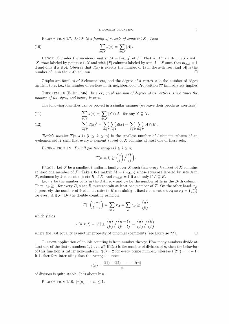
Figure 1. A convex function.
Then, the graph H obtained from G by deleting x and its incident edge has |V | − 1 = n verticesand |E| − 1 ≤ (n − 1) − 1 = n − 2 edges; by the induction hypothesis, H is disconnected. Therestoration of an edge joining a vertex y in one component to a vertex x which is outside of asecond component cannot reconnect the graph. Hence, G is also disconnected.
We mention one important inequality, which is especially useful when dealing with averages.A real-valued function f(x) is convex if
f(λa + (1 − λ)b) ≤ λf(a) + (1 − λ)f(b) ,
for any 0 ≤ λ ≤ 1. From a geometrical point of view, the convexity of f means that if we draw aline l through points (a, f(a)) and (b, f(b)), then the graph of the curve f(z) must lie below thatof l(z) for z ∈ [a, b]. Thus, for a function f to be convex it is sufficient that its second derivativeis nonnegative.
Proposition 1.12 (Jensen’s Inequality). If 0 ≤ λi ≤ 1,∑n
i=1 λi = 1 and f is convex, then
(14) f
( n∑
i=1
λixi
)≤
n∑
i=1
λif(xi) .
Proof. Easy induction on the number of summands n. For n = 2 this is true, so assume theinequality holds for the number of summands up to n, and prove it for n + 1. For this it is enoughto replace the sum of the first two terms in λ1x1 + λ2x2 + . . . + λn+1xn+1 by the term
(λ1 + λ2)
(λ1
λ1 + λ2x1 +
λ2
λ1 + λ2x2
),
and apply the induction hypothesis.
If a1, . . . , an are non-negative then, taking f(x) = x2 and λi = 1/n, we obtain a usefulinequality (which is also an easy consequence of the Cauchy–Schwarz inequality):
(15)
n∑
i=1
a2i ≥ 1
n
( n∑
i=1
ai
)2
.
Jensen’s inequality (??) yields the following useful inequality between the arithmetic andgeometric means: for any be non-negative numbers a1, . . . , an,
(16)1
n
n∑
i=1
ai ≥( n∏
i=1
ai
)1/n
.
To show this, apply Jensen’s inequality with f(x) = 2x, λ1 = . . . = λn = 1/n and xi = log2 ai, forall i = 1, . . . , n. Then
1
n
n∑
i=1
ai =n∑
i=1
λif(xi) ≥ f
(n∑
i=1
λixi
)= 2(
∑n
i=1xi)/n =
(n∏
i=1
ai
)1/n
.

10 1. COUNTING
6. The inclusion-exclusion principle
The principle of inclusion and exclusion (sieve of Eratosthenes) is a powerful tool in the theoryof enumeration as well as in number theory. This principle relates the cardinality of the union ofcertain sets to the cardinalities of intersections of some of them, these latter cardinalities oftenbeing easier to handle.
For any two sets A and B we have
|A ∪ B| = |A| + |B| − |A ∩ B|.In general, given n subsets A1, . . . , An of a set X, we want to calculate the number |A1 ∪ · · · ∪ An|of points in their union. As the first approximation of this number we can take the sum
(17) |A1| + · · · + |An|.However, in general, this number is too large since if, say, Ai ∩ Aj 6= ∅ then each point of Ai ∩ Aj
is counted two times in (??): once in |Ai| and once in |Aj |. We can try to correct the situationby subtracting from (??) the sum
(18)∑
1≤i<j≤n
|Ai ∩ Aj |.
But then we get a number which is too small since each of the points in Ai ∩ Aj ∩ Ak 6= ∅ iscounted three times in (??): once in |Ai ∩ Aj |, once in |Aj ∩ Ak|, and once in |Ai ∩ Ak|. We cantherefore try to correct the situation by adding the sum
∑
1≤i<j<k≤n
|Ai ∩ Aj ∩ Ak|,
but again we will get a too large number, etc. Nevertheless, it turns out that after n steps we willget the correct result. This result is known as the inclusion-exclusion principle. The followingnotation will be handy: if I is a subset of the index set 1, . . . , n, we set
AI :=⋂
i∈I
Ai,
with the convention that A∅ = X.
Proposition 1.13 (Inclusion-Exclusion Principle). Let A1, . . . , An be subsets of X. Then thenumber of elements of X which lie in none of the subsets Ai is
(19)∑
I⊆1,...,n(−1)|I||AI |.
Proof. The sum is a linear combination of cardinalities of sets AI with coefficients +1 and−1. We can re-write this sum as
∑
I
(−1)|I||AI | =∑
I
∑
x∈AI
(−1)|I| =∑
x
∑
I:x∈AI
(−1)|I|.
We calculate, for each point of X, its contribution to the sum, that is, the sum of the coefficientsof the sets AI which contain it.
First suppose that x ∈ X lies in none of the sets Ai. Then the only term in the sum to whichx contributes is that with I = ∅; and this contribution is 1.
Otherwise, the set J := i : x ∈ Ai is non-empty; and x ∈ AI precisely when I ⊆ J . Thus,the contribution of x is
∑
I⊆J
(−1)|I| =
|J|∑
i=0
(|J |i
)(−1)i = (1 − 1)|J| = 0
by the binomial theorem.Thus, points lying in no set Ai contribute 1 to the sum, while points in some Ai contribute 0;
so the overall sum is the number of points lying in none of the sets, as claimed.

6. THE INCLUSION-EXCLUSION PRINCIPLE 11
For some applications the following form of the inclusion-exclusion principle is more conve-nient.
Proposition 1.14. Let A1, . . . , An be a sequence of (not necessarily distinct) sets. Then
(20) |A1 ∪ · · · ∪ An| =∑
∅6=I⊆1,...,n(−1)|I|+1|AI | .
Proof. The left-hand of (??) is |A∅| minus the number of elements of X = A∅ which lie innone of the subsets Ai. By Proposition ?? this number is
|A∅| −∑
I⊆1,...,n(−1)|I||AI | =
∑
∅6=I⊆1,...,n(−1)|I|+1|AI | ,
as desired.
Suppose we would like to know, given a set of indices I, how many elements belong to allthe sets Ai with i ∈ I and do not belong to any of the remaining sets. Proposition ?? (whichcorresponds to the case when I = ∅) can be generalized for this situation.
Proposition 1.15. Let A1, . . . , An be sets, and I a subset of the index set 1, . . . , n. Thenthe number of elements which belong to Ai for all i ∈ I and for no other values is
(21)∑
J⊇I
(−1)|J\I||AJ | .
Proof. Consider the set X :=⋂
i∈I Ai and its subsets Bk := X ∩ Ak, for all k ∈ N \ I, whereN := 1, . . . , n. The proposition asks us to calculate the number of elements of X lying in noneof Bk. By Proposition ??, this number is
∑
K⊆N\I
(−1)|K|∣∣∣∣⋂
k∈K
Bk
∣∣∣∣ =∑
K⊆N\I
(−1)|K|∣∣∣∣⋂
i∈K∪I
Ai
∣∣∣∣
=∑
J⊇I
(−1)|J\I||AJ | .
What is the probability that if n people randomly search a dark closet to retrieve their hats,no person will pick his own hat? Using the principle of inclusion and exclusion it can be shownthat this probability is very close to e−1 = 0.3678....
This question can be formalized as follows. A permutation is a bijective mapping f of theset 1, . . . , n into itself. We say that f fixes a point i if f(i) = i. A derangement is a permu-tation which fixes none of the points. We have exactly n! permutations. How many of them arederangements?
Proposition 1.16. The number of derangements of 1, . . . , n is equal to
(22)
n∑
i=0
(−1)i
(n
i
)(n − i)! = n!
n∑
i=0
(−1)i
i!.
The sum∑n
i=0(−1)i
i! is the initial part of the Taylor expansion of e−1; so about an e−1 fractionof all permutations are derangements.
Proof. We are going to apply the inclusion-exclusion formula (??). Let X be the set ofall permutations, and Ai the set of permutations fixing the point i; so |Ai| = (n − 1)!, and moregenerally, |AI | = (n−|I|)!, since permutations in AI fix every point in I and permute the remainingpoints arbitrarily. A permutation is a derangement if and only if it lies in none of the sets Ai; soby (??), the number of derangements is
∑
I⊆1,...,n(−1)|I|(n − |I|)! =
n∑
i=0
(−1)i
(n
i
)(n − i)!
putting i = |I|.

12 1. COUNTING
Exercises
Ex 1.1. In how many ways can we distribute k balls to n boxes so that each box has at mostone ball?
Ex 1.2. Show that for every k the product of any k consecutive natural numbers is divisibleby k!. Hint: Consider
(n+k
k
).
Ex 1.3. Show that the number of pairs (A, B) of distinct subsets of 1, . . . , n with A ⊂ B is3n − 2n. Hint: Use the binomial theorem to evaluate
∑n
k=0
(nk
)(2k − 1).
Ex 1.4. Show that (n
k
)=
n
k
(n − 1
k − 1
).
Hint: Count in two ways the number of pairs (x, M), where M is a k-element subset of 1, . . . , nand x ∈ M .
Ex 1.5. Prove thatn∑
k=1
k
(n
k
)= n2n−1 .
Hint: Count in two ways the number of pairs (x, M) with x ∈ M ⊆ 1, . . . , n.
Ex 1.6. There is a set of 2n people: n male and n female. A good party is a set with thesame number of male and female. How many possibilities are there to build such a good party?
Ex 1.7. Use Proposition ?? to show thatr∑
i=0
(n + i − 1
i
)=
(n + r
r
).
Ex 1.8. Let 0 ≤ a ≤ m ≤ n be integers. Use Proposition ?? to show thatn∑
i=m
(i
a
)=
(n + 1
a + 1
)−(
m
a + 1
).
Ex 1.9. Prove the Cauchy–Vandermonde identity:(
p + q
k
)=
k∑
i=0
(p
i
)(q
k − i
).
Hint: Take a set of p + q people (p male and q female) and make a set of k people (with i male and k − i
female).
Ex 1.10. Show thatn∑
k=0
(n
k
)2
=
(2n
n
).
Hint: Exercise ?? and Eq. (??).
Ex 1.11. Prove the following analogy of the binomial theorem for factorials:
(x + y)n =
n∑
k=0
(n
k
)(x)k(y)n−k .
Hint: Divide both sides by n!, and use the Cauchy–Vandermonde identity.
Ex 1.12. Let 0 ≤ l ≤ k ≤ n. Show that(
n
k
)(k
l
)=
(n
l
)(n − l
k − l
).
Hint: Count in two ways the number of all pairs (L, K) of subsets of 1, . . . , n such that L ⊆ K, |L| = l
and |K| = k.

EXERCISES 13
Ex 1.13. Use combinatorics (not algebra) to prove that, for 0 ≤ k ≤ n,(
n
2
)=
(k
2
)+ k(n − k) +
(n − k
2
).
Hint:(
n2
)is the number of edges in a complete graph on n vertices.
Ex 1.14. One of Euclid’s theorems says that, if a prime number divides a product a · b of twointegers, then p must divide at least one of these integers. Use this to show that:
(i) If 1 ≤ k < p, then(
pk
)≡ 0 mod p.
(ii) If 1 ≤ k ≤ n < p, then(
nk
)6≡ 0 mod p.
Hint: (i) Let x = n(n − 1) · · · (n − k + 1). Note that x = a · b with a =(
nk
)and b = k!.
Ex 1.15. Prove Fermat’s Little theorem: if p is a prime and if a is a natural number, thenap ≡ a mod p. In particular, if p does not divide a, then ap−1 ≡ 1 mod p. Hint: Apply the inductionon a. For the induction step, use the binomial theorem to show that (a + 1)p ≡ ap + 1 mod p.
Ex 1.16. Let 0 < α < 1 be a real number, and αn be an integer. Using Stirling’s formulashow that (
n
αn
)=
1 + o(1)√2πα(1 − α)n
· 2n·H(α),
where H(α) = −α log2 α−(1−α) log2(1−α) is the binary entropy function. Hint: H(α) = log2 h(α),where h(α) = α−α(1 − α)−(1−α).
Ex 1.17. Prove that, for s ≤ n/2,
(1):
s∑
k=0
(n
k
)≤(
n
s
)(1 +
s
n − 2s + 1
);
(2):
s∑
k=0
(n
k
)≤ 2n·H(s/n).
Hint: To (1): observe that(
nk−1
)/(
nk
)= k/(n − k + 1) does not exceed α := s/(n − s + 1), and use the
identity∑∞
i=0αi = 1/(1 − α).
To (2): set p = s/n and apply the binomial theorem to show that
ps(1 − p)n−s
s∑
k=0
(n
k
)≤ 1 .
See also Corollary ?? for another proof.
Ex 1.18. Prove the following estimates: If k ≤ k + x < n and y < k ≤ n, then
(23)
(n − k − x
n − x
)x
≤(
n − x
k
)(n
k
)−1
≤(
n − k
n
)x
≤ e−(k/n)x
and (k − y
n − y
)y
≤(
n − y
k − y
)(n
k
)−1
≤(
k
n
)y
.
Ex 1.19. Prove that if 1 ≤ k ≤ n/2, then
(24)
(n
k
)≥ γ ·
(ne
k
)k
, where γ =1√2πk
e−k2/n−1/(6k).
Hint: Use Stirling’s formula to show that(
n
k
)≥ 1√
2π e1/(6k)
(n
k
)k ( n
n − k
)n−k(
n
k(n − k)
)1/2
,
and apply the estimate ln(1 + t) ≥ t − t2/2 valid for all t ≥ 0.
Ex 1.20. In how many ways can we choose a subset S ⊆ 1, 2, . . . , n such that |S| = k andno two elements of S precede each other, i.e., x 6= y + 1 for all x, y ∈ S? Hint: If S = a1, . . . , akis such a subset with a1 < a2 < . . . < ak, then a1 < a2 − 1 < . . . < ak − (k − 1).
14 1. COUNTING
Ex 1.21. Let k ≥ 2n. In how many ways can we distribute k sweets to n children, if eachchild is supposed to get at least 2 of them?
Ex 1.22. Let F = A1, . . . , Am be a family of subsets of a finite set X. For x ∈ X, let d(x)be the number of members of F containing x. Show that
∑mi,j=1 |Ai ∩ Aj | =
∑x∈X d(x)2.
Ex 1.23. Bell’s number Bn is the number of all possible partitions of an n-element set X(we assume that B0 = 1). Prove that Bn+1 =
∑ni=0
(ni
)Bi. Hint: For every subset A ⊆ X there are
precisely B|X\A| partitions of X containing A as one of its blocks.
Ex 1.24. Let |N | = n and |X| = x. Show that there are xn mappings from N to X, andthat S(n, k)x(x − 1) · · · (x − k + 1) of these mappings have a range of cardinality k; here S(n, k)is the Stirling number (the number of partitions of an n-element set into exactly k blocks). Hint:We have x(x − 1) · · · (x − k + 1) possibilities to choose a sequence of k elements in X, and we can specifyS(n, k) ways in which elements of N are mapped onto these chosen elements.
Ex 1.25. Let F be a family of subsets of an n-element set X with the property that any twomembers of F meet, i.e., A ∩ B 6= ∅ for all A, B ∈ F . Suppose also that no other subset of Xmeets all of the members of F . Prove that |F| = 2n−1. Hint: Consider sets and their complements.
Ex 1.26. Let F be a family of k-element subsets of an n-element set X such that every l-element subset of X is contained in at least one member of F . Show that |F| ≥
(nl
)/(kl
). Hint:
Argue as in the proof of Proposition ??.
Ex 1.27. (Sperner 1928). Let F be a family of k-element subsets of 1, . . . , n. Its shadow isthe family of all those (k−1)-element subsets which lie entirely in at least one member of F . Showthat the shadow contains at least k|F|/(n−k+1) sets. Hint: Argue as in the proof of Proposition ??.
Ex 1.28. (Counting in bipartite graphs). Let G = (A ∪ B, E) be a bipartite graph, d be aminimum degree of a vertex in A and D the maximum degree of a vertex in B. Assume that|A|d ≥ |B|D. Show that then, for every subset A0 ⊆ A of density α := |A0|/|A|, there is a subsetB0 ⊆ B such that: (i) |B0| ≥ α|B|/2, (ii) every vertex of B0 has at least αD/2 neighbors in A0,and (iii) at least half of the edges leaving A0 go to B0. Hint: Let B0 consist of all vertices in B having> αD/2 neighbors in A0.
Ex 1.29. Let a1, . . . , an be nonnegative numbers. Define
f(t) =
(at
1 + · · · + atn
n
)1/t
.
Use Jensen’s inequality to show that s ≤ t implies f(s) ≤ f(t).
Ex 1.30. (Quine 1988). The famous Fermat’s Last Theorem states that if n > 2, thenxn + yn = zn has no solutions in nonzero integers x, y and z. This theorem can be stated in termsof sorting objects into a row of bins, some of which are red, some blue, and the rest unpainted. Thetheorem amounts to saying that when there are more than two objects, the following statementis never true: The number of ways of sorting them that shun both colors is equal to the number ofways that shun neither. Show that this statement is equivalent to Fermat’s equation xn +yn = zn.Hint: Let n be the number of objects, z the number of bins, x the number of bins that are not red and y
the number of bins that are not blue. There are zn ways of sorting the objects into bins; xn of these waysshun red and yn of them shun blue.
Ex 1.31. Use the principle of inclusion and exclusion to determine the number of ways inwhich three women and their three spouses may be seated around a round table under each of thefollowing two restrictions:
(i) no woman sits beside her spouse (on either side);(ii) no two women may sit opposite one another at the table (i.e., with two people between them
on either side).

EXERCISES 15
Hint: To (i): two seatings are equivalent if one can be rotated into the other; so the underlying set consistsof all circular permutations, 5! in number. Let Ai (i = 1, 2, 3) be the subset of permutations in which themembers of the i-th couple sit side by side. Show that |Ai| = 2 ·4!, |Ai ∩Aj | = 22 ·3!, |A1 ∩A2 ∩A3| = 23 ·2!and apply the inclusion-exclusion formula. To (ii): distinguish two cases, according to whether thereexist two women sitting side by side or not.
Ex 1.32. Let m ≥ n. A function f : [m] → [n] is a surjection (or a mapping of [m] onto [n]) iff maps at least one element of [m] to each element of [n]. Prove that the number of such functions
is∑n−1
k=0(−1)k(
nk
)(n − k)m. Hint: Let Ai = f : f(j) 6= i for all j and apply the inclusion-exclusion
formula.
Ex 1.33. Let n and k ≥ l be positive integers. How many different integer solutions are thereto the equation x1 +x2 + · · ·+xn = k, with all 0 ≤ xi < l? Hint: Consider the universum X = Xn,k ofall solutions with all xi ≥ 0, let Ai be the set of all solutions with xi ≥ l, and apply the inclusion-exclusionformula (??). Observe that |Ai| = |Xn,k−l|, where the size of Xn,k is given by Proposition ??.
Ex 1.34. Let r ≥ 5. How many ways are there to color the vertices with r colors in thefollowing graphs such that adjacent vertices get different colors?
Hint: For the first graph, the universe X is the set of all r4 ways to color the vertices. Associatewith each edge e the set Ae of all colorings, which assign the same color to its ends, and apply theinclusion-exclusion formula (??).
Ex 1.35. Say that a permutation π on [2n] has property P if for some i ∈ [2n], |π(i)−π(i+1)| =n, where i+1 is taken modulo 2. Show that, for each n, there are more permutations with propertyP than without it. Hint: Consider the sets Ai = π : |π(i)−π(i+1)| = n. Show that |Ai| = 2n(2n−2)!and Ai ∩ Ai+1 = ∅.
Ex 1.36. Prove that for any two sets I ⊆ J ,∑
I⊆K⊆J
(−1)|K\I| =
1, if I = J0, if I 6= J.
Ex 1.37. Prove the following Bonferroni inequalities for each even k ≥ 2:
k∑
ν=1
(−1)ν+1∑
|I|=ν
|AI | ≤ |n⋃
i=1
Ai| ≤k+1∑
ν=1
(−1)ν+1∑
|I|=ν
|AI |
where AI :=⋂
i∈I Ai. What about an odd k?
Ex 1.38. Let M be an n × n boolean matrix (with entries 0 and 1). A covering of M is a setR1, . . . , Rt of rank-1 boolean matrices such that every 1-entry of M is a 1-entry in at least one ofthese matrices, and every 0-entry of M is a 0-entry in all these matrices. That is, M must be anentry-wise Or M =
∨ti=1 Ri of the Ri’s. Let t(A) be the smallest number of the Ri’s in such a
covering of M . For a boolean matrix B ≤ M (again, inequality is entry-wise), let wM (B) denotethe largest possible number of 1-entries in B that can be covered by some all-1 submatrix R ofM . (Note that R need not be a submatrix of B.) Set
µ(M) = maxB≤M
|B|wM (B)
,
where |B| is the number of 1s in B. Prove that
µ(M) ≤ t(M) ≤ µ(M) · ln |M | + 1 .
Hint: For the upper bound, consider a greedy covering R1, ..., Rt of M by all-1 submatrices: in the i-thstep choose an all-1 submatrix Ri ≤ M covering the largest number of all yet uncovered 1s in M . LetBi ≤ M be the submatrix containing all 1-entries of M that are left uncovered after the i-th step. Observethat |Bi|/wA(Bi) ≤ µ(A) for all i.

16 1. COUNTING
Ex 1.39. For a boolean matrix M and an integer k ≥ 1, let tk(M) denote the smallest number
t of rank-1 boolean matrices R1, . . . , Rt in a covering of M with a restriction that∑t
i=1 Ri ≤ kJ ,where J is an all-1 matrix. That is, we now require that no 1-entry of M is covered more than ktimes. Prove that then
k∑
i=1
(t
i
)≥ rk(M) .
Hint: For a subset I ⊆ 1, . . . , t, let RI be a (0, 1) matrix with RI [x, y] = 1 iff Ri[x, y] = 1 for all i ∈ I.Use the inclusion-exclusion principle to write M as
M =∑
I 6=∅
(−1)|I|+1RI .
Ex 1.40. The determinant det(A) of an n × n matrix A = (aij) is a sum of n! signed products±a1i1
a2i2· · · anin
, where (i1, i2, . . . , in) is a permutation of (1, 2, . . . , n), the sign being +1 or −1,according to whether the number of inversions of (i1, i2, . . . , in) is even or odd. An inversionoccurs when ir > is but r < s. Prove the following: let A be a matrix of even order n with 0s onthe diagonal and arbitrary entries from +1, −1 elsewhere. Then det(A) 6= 0. Hint: Observe thatfor such matrices, det(A) is congruent modulo 2 to the number of derangements on n points, and showthat for even n, the sum (??) is odd.
CHAPTER 2
Advanced Counting
When properly applied, the (double) counting argument can lead to more subtle results thanthose discussed in the previous chapter.
1. Bounds on intersection size
How many r-element subsets of an n-element set can we choose under the restriction thatno two of them share more than k elements? Intuitively, the smaller k is, the fewer sets we canchoose. This intuition can be made precise as follows. (We address the optimality of this boundin Exercise ??.)
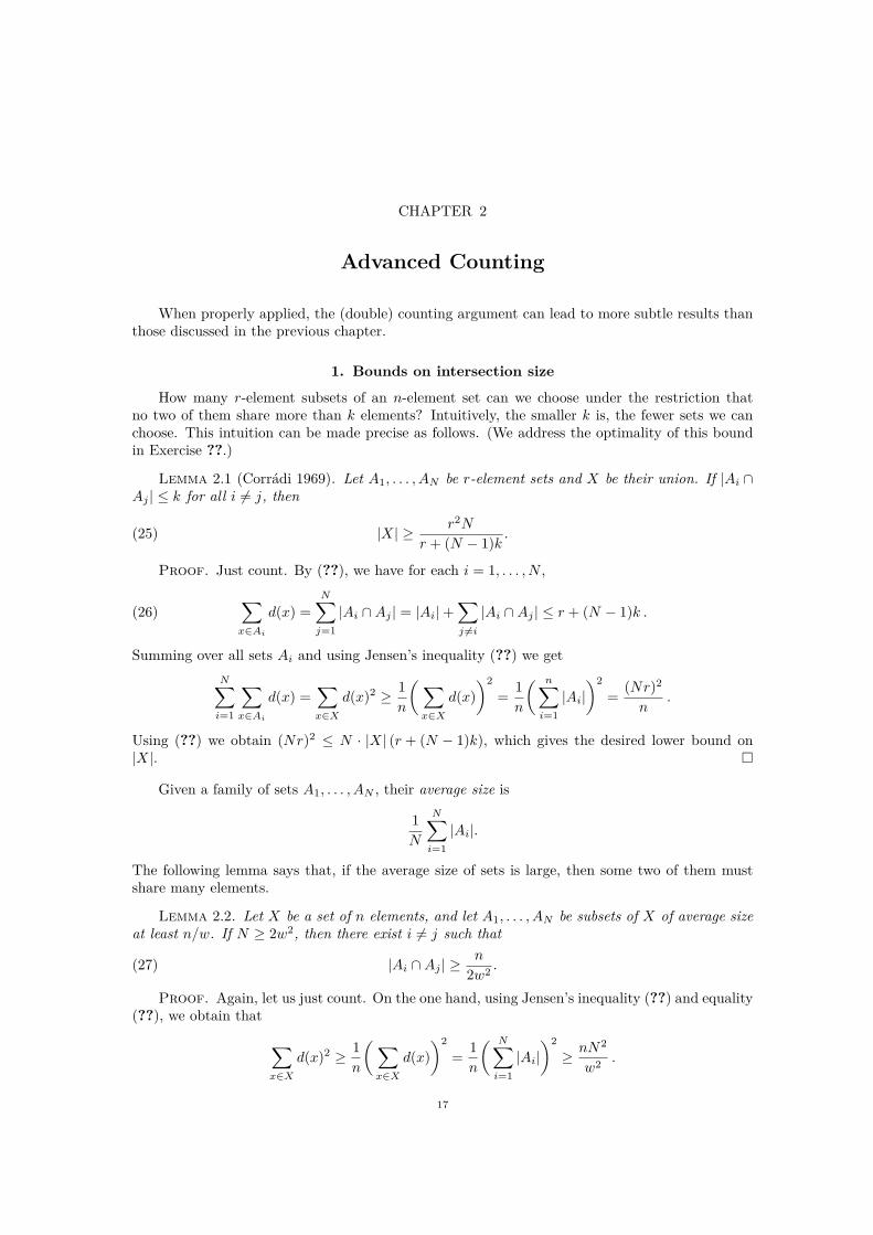
Lemma 2.1 (Corrádi 1969). Let A1, . . . , AN be r-element sets and X be their union. If |Ai ∩Aj | ≤ k for all i 6= j, then
(25) |X| ≥ r2N
r + (N − 1)k.
Proof. Just count. By (??), we have for each i = 1, . . . , N ,
(26)∑
x∈Ai
d(x) =N∑
j=1
|Ai ∩ Aj | = |Ai| +∑
j 6=i
|Ai ∩ Aj | ≤ r + (N − 1)k .
Summing over all sets Ai and using Jensen’s inequality (??) we get
N∑
i=1
∑
x∈Ai
d(x) =∑
x∈X
d(x)2 ≥ 1
n
(∑
x∈X
d(x)
)2
=1
n
( n∑
i=1
|Ai|)2
=(Nr)2
n.
Using (??) we obtain (Nr)2 ≤ N · |X| (r + (N − 1)k), which gives the desired lower bound on|X|.
Given a family of sets A1, . . . , AN , their average size is
1
N
N∑
i=1
|Ai|.
The following lemma says that, if the average size of sets is large, then some two of them mustshare many elements.
Lemma 2.2. Let X be a set of n elements, and let A1, . . . , AN be subsets of X of average sizeat least n/w. If N ≥ 2w2, then there exist i 6= j such that
(27) |Ai ∩ Aj | ≥ n
2w2 .
Proof. Again, let us just count. On the one hand, using Jensen’s inequality (??) and equality(??), we obtain that
∑
x∈X
d(x)2 ≥ 1
n
(∑
x∈X
d(x)
)2
=1
n
( N∑
i=1
|Ai|)2
≥ nN2
w2 .
17

18 2. ADVANCED COUNTING
On the other hand, assuming that (??) is false and using (??) and (??) we would obtain
∑
x∈X
d(x)2 =
N∑
i=1
N∑
j=1
|Ai ∩ Aj | =∑
i
|Ai| +∑
i6=j
|Ai ∩ Aj |
< nN +nN(N − 1)
2w2 =nN2
2w2
(1 +
2w2
N− 1
N
)≤ nN2
w2 ,
a contradiction.
Lemma ?? is a very special (but still illustrative) case of the following more general result.
Lemma 2.3 (Erdős 1964b). Let X be a set of n elements x1, . . . , xn, and let A1, . . . , AN be Nsubsets of X of average size at least n/w. If N ≥ 2kwk, then there exist Ai1
, . . . , Aiksuch that
|Ai1∩ · · · ∩ Aik
| ≥ n/(2wk).
The proof is a generalization of the one above and we leave it as an exercise (see Exercises ??and ??).
2. Graphs with no 4-cycles
Let H be a fixed graph. A graph is H-free if it does not contain H as a subgraph. (Recallthat a subgraph is obtained by deleting edges and vertices.) A typical question in graph theory isthe following one:
How many edges can a H-free graph with n vertices have?
That is, one is interested in the maximum number ex(n, H) of edges in a H-free graph on nvertices. The graph H itself is then called a “forbidden subgraph.”
Let us consider the case when forbidden subgraphs are cycles. Recall that a cycle Ck of lengthk (or a k-cycle) is a sequence v0, v1, . . . , vk such that vk = v0 and each subsequent pair vi and vi+1
is joined by an edge.If H = C3, a triangle, then ex(n, C3) ≥ n2/4 for every even n ≥ 2: a complete bipartite r × r
graph Kr,r with r = n/2 has no triangles but has r2 = n2/4 edges. We will show later that thisis already optimal: any n-vertex graph with more than n2/4 edges must contain a triangle (seeTheorem ??). Interestingly, ex(n, C4) is much smaller, smaller than n3/2.
Theorem 2.4 (Reiman 1958). If G = (V, E) on n vertices has no 4-cycles, then
|E| ≤ n
4(1 +
√4n − 3) .
Proof. Let G = (V, E) be a C4-free graph with vertex-set V = 1, . . . , n, and d1, d2, . . . , dn
be the degrees of its vertices. We now count in two ways the number of elements in the followingset S. The set S consists of all (ordered) pairs (u, v, w) such that v 6= w and u is adjacent toboth v and w in G. That is, we count all occurrences of “cherries”
w
uv
in G. For each vertex u, we have(
du
2
)possibilities to choose a 2-element subset of its du neighbors.
Thus, summing over u, we find |S| =∑n
u=1
(du
2
). On the other hand, the C4-freeness of G implies
that no pair of vertices v 6= w can have more than one common neighbor. Thus, summing over allpairs we obtain that |S| ≤
(n2
). Altogether this gives
n∑
i=1
(di
2
)≤(
n
2
)
or
(28)
n∑
i=1
d2i ≤ n(n − 1) +
n∑
i=1
di .

3. GRAPHS WITH NO INDUCED 4-CYCLES 19
G
Figure 1. Graph G contains several copies of C4 as a subgraph, but none ofthem as an induced subgraph.
Now, we use the Cauchy–Schwarz inequality( n∑
i=1
xiyi
)2
≤( n∑
i=1
x2i
)( n∑
i=1
y2i
)
with xi = di and yi = 1, and obtain( n∑
i=1
di
)2
≤ n
n∑
i=1
d2i
and hence by (??) ( n∑
i=1
di
)2
≤ n2(n − 1) + nn∑
i=1
di .
Euler’s theorem gives∑n
i=1 di = 2|E|. Invoking this fact, we obtain
4|E|2 ≤ n2(n − 1) + 2n|E|or
|E|2 − n
2|E| − n2(n − 1)
4≤ 0 .
Solving the corresponding quadratic equation yields the desired upper bound on |E|.
Example 2.5 (Construction of dense C4-free graphs). The following construction shows thatthe bound of Theorem ?? is optimal up to a constant factor.
Let p be a prime number and take V = (Zp \ 0) × Zp, that is, vertices are pairs (a, b) ofelements of a finite field with a 6= 0. We define a graph G on these vertices, where (a, b) and (c, d)are joined by an edge iff ac = b + d (all operations modulo p). For each vertex (a, b), there arep − 1 solutions of the equation ax = b + y: pick any x ∈ Zp \ 0, and y is uniquely determined.Thus, G is a (p − 1)-regular graph on n = p(p − 1) vertices (some edges are loops). The numberof edges in it is n(p − 1)/2 = Ω(n3/2).
To verify that the graph is C4-free, take any two its vertices (a, b) and (c, d). The uniquesolution (x, y) of the system
ax = b + ycx = d + y
is given byx = (b − d)(a − c)−1
2y = x(a + c) − b − d
which is only defined when a 6= c, and has x 6= 0 only when b 6= d. Hence, if a 6= c and b 6= d, thenthe vertices (a, b) and (c, d) have precisely one common neighbor, and have no common neighborsat all, if a = c or b = d.
3. Graphs with no induced 4-cycles
Recall that an induced subgraph is obtained by deleting vertices together with all the edgesincident to them (see Fig. ??).
Theorem ?? says that a graph cannot have many edges, unless it contains C4 as a (notnecessarily induced) subgraph. But what about graphs that do not contain C4 as an inducedsubgraph? Let us call such graphs weakly C4-free.
Note that such graphs can already have many more edges. In particular, the complete graphKn is weakly C4-free: in any 4-cycle there are edges in Kn between non-neighboring vertices of C4.Interestingly, any(!) dense enough weakly C4-free graph must contain large complete subgraphs.

20 2. ADVANCED COUNTING
[rgb]0,0,0
.
.
.
.
.
.
.
.
.
.
.
.
.
.
.
.
.
.
.
.
.
.
.
.
.
.
.
.
.
.
.
.
.
.
.
.
.
.
.
.
.
.
.
.
.
.
.
.
.
.
.
.
.
.
.
.
.
.
.
.
.
.
...............
.
.
.
.
.
.
.
.
.
.
.
.
.
.
.
.
.
.
.
.
.
.
.
.
.
.
.
.
.
.
.
.
.
.
.
.
.
.
.
.
.
.
.
.
.
.
.
.
.
.
.
.
.
.
.
.
.
.
.
.
.
.
.
.
.
.
.
.
.
.
.
.
.
.
.
.
.
.
.
.
.
.
.
.
.
.
.
.
.
.
.
.
.
.
.
.
.
.
.
.
.
.
.
.
.
.
.
.
.
.
.
.
.
.
.
.
.
.
.
.
.
.
.
............................................................................
[rgb]0,0,0
.
.
.
.
.
.
.
.
.
.
.
.
.
.
.
.
.
.
.
.
.
.
.
.
.
.
.
.
.
.
.
.
.
.
.
.
.
.
.
.
.
.
.
.
.
.
.
.
.
.
.
.
.
.
.
.
.
.
.
.
.
.
...............
.
.
.
.
.
.
.
.
.
.
.
.
.
.
.
.
.
.
.
.
.
.
.
.
.
.
.
.
.
.
.
.
.
.
.
.
.
.
.
.
.
.
.
.
.
.
.
.
.
.
.
.
.
.
.
.
.
.
.
.
.
.
.
.
.
.
.
.
.
.
.
.
.
.
.
.
.
.
.
.
.
.
.
.
.
.
.
.
.
.
.
.
.
.
.
.
.
.
.
.
.
.
.
.
.
.
.
.
.
.
.
.
.
.
.
.
.
.
.
.
.
.
.
.............................................................................
[rgb]0,0,0
.
.
.
.
.
.
.
.
.
.
.
.
.
.
.
.
.
.
.
.
.
.
.
.
.
.
.
.
.
.
.
.
.
.
.
.
.
.
.
.
.
.
.
.
.
.
.
.
.
.
.
.
.
.
.
.
.
.
.
.
.
.
.
.
.
.
.
.
.
.
.
.
.
.
.
.
.
.
.
.
.
.
.
.
.
.
.
.
.
.
.
.
.
.
.
.
.
.
.
.
.
.
.
.
.
.
.
.
.
.
.
.
.
.
.
.
...................
.
.
.
.
.
.
.
.
.
.
.
.
.
.
.
.
.
.
.
.
.
.
.
.
.
.
.
.
.
.
.
.
.
.
.
.
.
.
.
.
.
.
.
.
.
.
.
.
.
.
.
.
.
.
.
.
.
.
.
.
.
.
.
.
.
.
.
.
.
.
.
.
.
.
.
.
.
.
.
.
.
.
.
.
.
.
.
.
.
.
.
.
.
.
.
.
.
.
.
.
.
.
.
.
.
.
.
.
.
.
.
.
.
.
.
.
.
.
.
.
.
.
.
.
.
.
.
.
.
.
.
.
.
.
.
.
.
.
.
.
.
.
.
.
.
.
.
.
.
.
.
.
.
.
.
.
.
.
.
.
.
.
.
.
.
.
.
.
.
.
.
.
.
.
.
.
.
.
.
.
.
.
.
.
.
.
.
.
.
.
.
.
.
.
.
.
.
.
.
.
.
.
.
.
.
.
.
.
.
.
.
.
.
.
.
.
.
.
.
.
.
.
.
.
.
.
.
.
.
.
.
......................................................................................................................................
[rgb]0,0,0
.
.
.
.
.
.
.
.
.
.
.
.
.
.
.
.
.
.
.
.
.
.
.
.
.
.
.
.
.
.
.
.
.
.
.
.
.
.
.
.
.
.
.
.
.
.
.
.
.
.
.
.
.
.
.
.
.
.
.
.
.
.
.
.
.
.
.
.
.
.
.
.
.
.
.
.
.
.
.
.
.
.
.
.
.
.
.
.
.
.
.
.
.
.
.
.
.
.
.
.
.
.
.
.
.
.
.
.
.
.
.
.
.
.
.
.
...................
.
.
.
.
.
.
.
.
.
.
.
.
.
.
.
.
.
.
.
.
.
.
.
.
.
.
.
.
.
.
.
.
.
.
.
.
.
.
.
.
.
.
.
.
.
.
.
.
.
.
.
.
.
.
.
.
.
.
.
.
.
.
.
.
.
.
.
.
.
.
.
.
.
.
.
.
.
.
.
.
.
.
.
.
.
.
.
.
.
.
.
.
.
.
.
.
.
.
.
.
.
.
.
.
.
.
.
.
.
.
.
.
.
.
.
.
.
.
.
.
.
.
.
.
.
.
.
.
.
.
.
.
.
.
.
.
.
.
.
.
.
.
.
.
.
.
.
.
.
.
.
.
.
.
.
.
.
.
.
.
.
.
.
.
.
.
.
.
.
.
.
.
.
.
.
.
.
.
.
.
.
.
.
.
.
.
.
.
.
.
.
.
.
.
.
.
.
.
.
.
.
.
.
.
.
.
.
.
.
.
.
.
.
.
.
.
.
.
.
.
.
.
.
.
.
.
.
.
.
.
.......................................................................................................................................
[rgb]0,0,0
.
.
.
..........................
[rgb]0,0,0
.
.
.
..........................
[rgb]0,0,0
.
.
.
..........................
[rgb]0,0,0
.
.
.
.
.
.
[rgb]0,0,0[rgb]0,0,0[rgb]0,0,0[rgb]0,0,0[rgb]0,0,0[rgb]0
Figure 2. (a) If u and v were non-adjacent, we would have an induced 4-cyclexi, xj , u, v. (b) If y and z were non-adjacent, then (S \ xi) ∪ y, z would bea larger independent set.
Let ω(G) denote the maximum number of vertices in a complete subgraph of G. In particular,ω(G) ≤ 3 for every C4-free graph. In contrast, for weakly C4-free graphs we have the followingresult, due to Gyárfás, Hubenko and Solymosi (2002).
Theorem 2.6. If an n-vertex graph G = (V, E) is weakly C4-free, then
ω(G) ≥ 0.4|E|2n3 .
The proof of Theorem ?? is based on a simple fact, relating the average degree with theminimum degree, as well as on two facts concerning independent sets in weakly C4-free graphs.
For a graph G = (V, E), let e(G) = |E| denote the number of its edges, dmin(G) the smallestdegree of its vertices, and dave(G) = 2e(G)/|V | the average degree. Note that, by Euler’s theorem,dave(G) is indeed the sum of all degrees divided by the total number of vertices.
Proposition 2.7. Every graph G has an induced subgraph H with
dave(H) ≥ dave(G) and dmin(H) ≥ 1
2dave(G) .
Proof. We remove vertices one-by-one. To avoid the danger of ending up with the emptygraph, let us remove a vertex v ∈ V if this does not decrease the average degree dave(G). Thus,we should have
dave(G − v) =2(e(G) − d(v))
|V | − 1≥ dave(G) =
2e(G)
|V |which is equivalent to d(v) ≤ dave(G)/2. So, when we stick, each vertex in the resulting graph Hhas minimum degree at least dave(G)/2.
Recall that a set of vertices in a graph is independent if no two of its vertices are adjacent.Let α(G) denote the largest number of vertices in such a set.
Proposition 2.8. For every weakly C4-free graph G on n vertices, we have
ω(G) ≥ n(α(G)+1
2
) .
Proof. Fix an independent set S = x1, . . . , xα with α = α(G). Let Ai be the set ofneighbors of xi in G, and Bi the set of vertices whose only neighbor in S is xi. Consider thefamily F consisting of all α sets xi ∪ Bi and
(α2
)sets Ai ∩ Aj . We claim that:
[(ii)]each member of F forms a clique in G, and the members of F cover allvertices of G.
The sets Ai ∩ Aj are cliques because G is weakly C4-free: Any two vertices u 6= v ∈ Ai ∩ Aj mustbe joined by an edge, for otherwise xi, xj , u, v would form a copy of C4 as an induced subgraph.The sets xi∪Bi are cliques because S is a maximal independent set: Otherwise we could replace
4. ZARANKIEWICZ’S PROBLEM 21
xi in S by any two vertices from Bi. By the same reason (S being a maximal independent set),the members of F must cover all vertices of G: If some vertex v were not covered, then S ∪ vwould be a larger independent set.
Claims (i) and (ii), together with the averaging principle, imply that
ω(G) ≥ n
|F| =n
α +(
α2
) =n(
α+12
) .
Proposition 2.9. Let G be a weakly C4-free graph on n vertices, and d = dmin(G). Then,for every t ≤ α(G),
ω(G) ≥ d · t − n(t2
) .
(i):(ii): Proof. Take an independent set S = x1, . . . , xt of size t and let Ai be the set ofneighbors of xi in G. Let m be the maximum of |Ai ∩ Aj | over all 1 ≤ i < j ≤ t. We already knowthat each Ai ∩ Aj must form a clique; hence, ω(G) ≥ m. On the other hand, by the Bonferroniinequality (Exercise ??) we have that
n ≥∣∣∣∣
t⋃
i=1
Ai
∣∣∣∣ ≥ td −∑
i<j
|Ai ∩ Aj | ≥ td −(
t
2
)m ,
from which the desired lower bound on ω(G) follows.
Now we are able to prove Theorem ??.
Proof of Theorem ??. Let a be the average degree of G; hence, a = 2|E|/n. By Propo-sition ??, we know that G has an induced subgraph of average degree ≥ a and minimum degree≥ a/2. So, we may assume w.l.o.g. that the graph G itself has these two properties. We nowconsider the two possible cases.
If α(G) ≥ 4n/a, then we apply Proposition ?? with∗ t = 4n/a and obtain
ω(G) ≥ (a/2) · t − n(t2
) =n(4n/a2
) .
If α(G) ≤ 4n/a, then we apply Proposition ?? and obtain
ω(G) ≥ n(α(G)+1
2
) ≥ n(4n/a+12
) .
In both cases we obtain
ω(G) ≥ n(4n/a+12
) =a2
8n + 2a≥ 0.1
a2
n.
4. Zarankiewicz’s problem
At most how many 1s can an n × n 0-1 matrix contain if it has no a × b submatrix whoseentries are all 1s? Zarankiewicz (1951) raised the problem of the estimation of this number fora = b = 3 and n = 4, 5, 6 and the general problem became known as Zarankiewicz’s problem.
It is worth reformulating this problem in terms of bipartite graphs. A bipartite graph withparts of size n is a triple G = (V1, V2, E), where V1 and V2 are disjoint n-element sets of vertices(or nodes), and E ⊆ V1 × V2 is the set of edges. We say that the graph contains an a × b cliqueif there exist an a-element subset A ⊆ V1 and a b-element subset B ⊆ V2 such that A × B ⊆ E.(Note that an a × b clique is not the same as a b × a clique, unless a = b.)
Let ka(n) be the minimal integer k such that any bipartite graph with parts of size n andmore than k edges contains at least one a × a clique. Using the probabilistic argument, it can beshown (see Exercise ??) that
ka(n) ≥ c · n2−2/a,
where c > 0 is a constant, depending only on a. It turns out that this bound is not very farfrom the best possible, and this can be proved using the double counting argument. The result
∗For simplicity, we ignore ceilings and floors.

22 2. ADVANCED COUNTING
is essentially due to Kővári, Sós and Turán (1954). For a = 2, a lower bound k2(n) ≤ 3n3/2 wasproved by Erdős (1938). He used this to prove that, if a set A ⊆ [n] is such that the productsof any two of its different members are different, then |A| ≤ π(n) + O(n3/4), where π(n) is thenumber of primes not exceeding n.
Theorem 2.10. For all natural numbers n ≥ a ≥ 2 we have
ka(n) ≤ (a − 1)1/an2−1/a + (a − 1)n.
Proof. The proof is a direct generalization of a double counting argument we used in theproof of Theorem ??. Our goal is to prove the following: let G = (V1, V2, E) be a bipartitegraph with parts of size n, and suppose that G does not contain an a × a clique; then |E| ≤(a − 1)1/an2−1/a + (a − 1)n.
By a star in the graph G we will mean a set of any a of its edges incident with one vertexx ∈ V1, i.e., a set of the form
S(x, B) := (x, y) ∈ E : y ∈ B,
where B ⊆ V2, |B| = a. Let ∆ be the total number of such stars in G. We may count the starsS(x, B) in two ways, by fixing either the vertex x or the subset B.
For a fixed subset B ⊆ V2, with |B| = a, we can have at most a − 1 stars of the form S(x, B),because otherwise we would have an a × a clique in G. Thus,
(29) ∆ ≤ (a − 1) ·(
n
a
).
On the other hand, for a fixed vertex x ∈ V1, we can form(
d(x)a
)stars S(x, B), where d(x) is the
degree of vertex x in G (i.e., the number of vertices adjacent to x). Therefore,
(30)∑
x∈V1
(d(x)
a
)≤ (a − 1) ·
(n
a
).
We are going to estimate the left-hand side from below using Jensen’s inequality. Unfortunately,the function
(xa
)= x(x−1) · · · (x−a+1)/a! is convex only for x ≥ a−1. But we can set f(z) :=
(xa
)
if x ≥ a−1, and f(x) := 0 otherwise. Then Jensen’s inequality (??) (with λx = 1/n for all x ∈ V1)yields
∑
x∈V1
(d(x)
a
)≥∑
x∈V1
f(d(x)) ≥ n · f( ∑
x∈V1
d(x)/n)
= n · f(|E|/n) .
If |E|/n < a − 1, there is nothing to prove. So, we can suppose that |E|/n ≥ a − 1. Then we havethat
n ·(|E|/n
a
)= n · f(|E|/n) ≤
∑
x∈V1
(d(x)
a
)≤ (a − 1)
(n
a
).
Expressing the binomial coefficients as quotients of factorials, this inequality implies
n (|E|/n − (a − 1))a ≤ (a − 1)na,
and therefore |E|/n ≤ (a − 1)1/an1−1/a + a − 1, from which the desired upper bound on |E|follows.
The theorem above says that any bipartite graph with many edges has large cliques. In orderto destroy such cliques we can try to remove some of their vertices. We would like to remove asfew vertices as possible. Just how few says the following result.
Theorem 2.11 (Ossowski 1993). Let G = (V1, V2, E) be a bipartite graph with no isolatedvertices, |E| < (k + 1)r edges and d(y) ≤ r for all y ∈ V2. Then we can delete at most k verticesfrom V1 so that the resulting graph has no (r − a + 1) × a clique for a = 1, 2, . . . , r.
For a vertex x, let N(x) denote the set of its neighbors in G, that is, the set of all verticesadjacent to x; hence, |N(x)| is the degree d(x) of x. We will use the following lemma relating thedegree to the total number of vertices.

5. DENSITY OF 0-1 MATRICES 23
Lemma 2.12. Let (X, Y, E) be a bipartite graph with no isolated vertices, and f : Y → [ 0, ∞)be a function. If the inequality d(y) ≤ d(x) · f(y) holds for each edge (x, y) ∈ E, then |X| ≤∑
y∈Y f(y).
Proof. By double counting,
|X| =∑
x∈X
∑
y∈N(x)
1
d(x)≤∑
x∈X
∑
y∈N(x)
f(y)
d(y)
=∑
y∈Y
∑
x∈N(y)
f(y)
d(y)=∑
y∈Y
f(y)
d(y)· |N(y)| =
∑
y∈Y
f(y).
Proof of Theorem ??. (Due to F. Galvin 1997). For a set of vertices Y ⊆ V2, letN(Y ) :=
⋂y∈Y N(y) denote the set of all its common neighbors in G, that is, the set of all those
vertices in V1 which are joined to each vertex of Y ; hence |N(Y )| ≤ r for all Y ⊆ V2. Let X ⊆ V1
be a minimal set with the property that |N(Y ) \ X| ≤ r − |Y | whenever Y ⊆ V2 and 1 ≤ |Y | ≤ r.Put otherwise, X is a minimal set of vertices in V1, the removal of which leads to a graph without(r − a + 1) × a cliques, for all a = 1, . . . , r.
Our goal is to show that |X| ≤ k.Note that, for each x ∈ X we can choose Yx ⊆ V2 so that 1 ≤ |Yx| ≤ r, x ∈ N(Yx) and
|N(Yx) \ X| = r − |Yx|;otherwise X could be replaced by X \ x, contradicting the minimality of X. We will applyLemma ?? to the bipartite graph G′ = (X, V2, F ), where
F = (x, y) : y ∈ Yx .
All we have to do is to show that the hypothesis of the lemma is satisfied by the function (hereN(y) is the set of neighbors of y in the original graph G):
f(y) :=|N(y)|
r,
because then
|X| ≤∑
y∈V2
f(y) =1
r
∑
y∈V2
|N(y)| =|E|r
< k + 1.
Consider an edge (x, y) ∈ F ; we have to show that d(y) ≤ d(x) · f(y), where
d(x) = |Yx| and d(y) = |x ∈ X : y ∈ Yx|are the degrees of x and y in the graph G′ = (X, V2, F ). Now, y ∈ Yx implies N(Yx) ⊆ N(y),which in its turn implies
|N(y) \ X| ≥ |N(Yx) \ X| = r − |Yx|;hence
d(y) ≤ |N(y) ∩ X| = |N(y)| − |N(y) \ X|≤ |N(y)| − r + |Yx| = r · f(y) − r + d(x),
and so
d(x) · f(y) − d(y) ≥ d(x) · f(y) − r · f(y) + r − d(x)
= (r − d(x)) · (1 − f(y)) ≥ 0 .
5. Density of 0-1 matrices
Let H be an m × n 0-1 matrix. We say that H is α-dense if at least an α-fraction of all itsmn entries are 1s. Similarly, a row (or column) is α-dense if at least an α-fraction of all its entriesare 1s.
The next result says that any dense 0-1 matrix must either have one “very dense” row or theremust be many rows which are still “dense enough.”

24 2. ADVANCED COUNTING
Lemma 2.13 (Grigni and Sipser 1995). If H is 2α-dense then either(a) there exists a row which is
√α-dense, or
(b) at least√
α · m of the rows are α-dense.
Note that√
α is larger than α when α < 1.
Proof. Suppose that the two cases do not hold. We calculate the density of the entire matrix.Since (b) does not hold, less than
√α · m of the rows are α-dense. Since (a) does not hold, each
of these rows has less than√
α · n 1s; hence, the fraction of 1s in α-dense rows is strictly less than(√
α)(√
α) = α. We have at most m rows which are not α-dense, and each of them has less thanαn ones. Hence, the fraction of 1s in these rows is also less than α. Thus, the total fraction of 1sin the matrix is less than 2α, contradicting the 2α-density of H.
Now consider a slightly different question: if H is α-dense, how many of its rows or columnsare “dense enough”? The answer is given by the following general estimate due to Johan Håstad.This result appeared in the paper of Karchmer and Wigderson (1990) and was used to provethat the graph connectivity problem cannot be solved by monotone circuits of logarithmic depth.
Suppose that our universe is a Cartesian product A = A1 × · · · × Ak of some finite setsA1, . . . , Ak. Hence, elements of A are strings a = (a1, . . . , ak) with ai ∈ Ai. Fix now a subset ofstrings H ⊆ A and a point b ∈ Ai. The degree of b in H is the number dH(b) = |a ∈ H : ai = b|of strings in H whose i-th coordinate is b.
Say that a point b ∈ Ai from the i-th set is popular in H if its degree dH(b) is at least a 1/2kfraction of the average degree of an element in Ai, that is, if
dH(b) ≥ 1
2k
|H||Ai|
.
Let Pi ⊆ Ai be the set of all popular points in the i-th set Ai, and consider the Cartesian productof these sets:
P := P1 × P2 × · · · × Pk .
Lemma 2.14 (Håstad). |P | > 12 |H|.
Proof. It is enough to show that |H \ P | < 12 |H|. For every non-popular point b ∈ Ai, we
have that
|a ∈ H : ai = b| <1
2k
|H||Ai|
.
Since the number of non-popular points in each set Ai does not exceed the total number of points|Ai|, we obtain
|H \ P | ≤k∑
i=1
∑
b 6∈Pi
|a ∈ H : ai = b| <k∑
i=1
∑
b 6∈Pi
1
2k
|H||Ai|
≤k∑
i=1
1
2k|H| =
1
2|H| .
Corollary 2.15. In any 2α-dense 0-1 matrix H either a√
α-fraction of its rows or a√
α-fraction of its columns (or both) are (α/2)-dense.
Proof. Let H be an m × n matrix. We can view H as a subset of the Cartesian product[m] × [n], where (i, j) ∈ H iff the entry in the i-th row and j-th column is 1. We are going toapply Lemma ?? with k = 2. We know that |H| ≥ 2αmn. So, if P1 is the set of all rows with atleast 1
4 |H|/|A1| = αn/2 ones, and P2 is the set of all columns with at least 14 |H|/|A2| = αm/2
ones, then Lemma ?? implies that
|P1|m
· |P2|n
≥ 1
2
|H|mn
≥ 1
2· 2αmn
mn= α .
Hence, either |P1|/m or |P2|/n must be at least√
α, as claimed.

6. THE LOVÁSZ–STEIN THEOREM 25
6. The Lovász–Stein theorem
This theorem was used by Stein (1974) and Lovász (1975) in studying some combinatorialcovering problems. The advantage of this result is that it can be used to get existence results forsome combinatorial problems using constructive methods rather than probabilistic methods.
Given a family F of subsets of some finite set X, its cover number of F , Cov (F), is theminimum number of members of F whose union covers all points (elements) of X.
Theorem 2.16. If each member of F has at most a elements, and each point x ∈ X belongsto at least v of the sets in F , then
Cov (F) ≤ |F|v
(1 + ln a) .
Proof. Let N = |X|, M = |F| and consider the N ×M 0-1 matrix A = (ax,i), where ax,i = 1iff x ∈ X belongs to the i-th member of F . By our assumption, each row of A has at least v onesand each column at most a ones. By double counting, we have that Nv ≥ Ma, or equivalently,
(31)M
v≤ N
a.
Our goal is to show that then A must contain an N × K submatrix C with no all-0 rows and suchthat
K ≤ N/a + (M/v) ln a ≤ (M/v)(1 + ln a) .
We describe a constructive procedure for producing the desired submatrix C. Let Aa = A anddefine A′
a to be any maximal set of columns from Aa whose supports† are pairwise disjoint andwhose columns each have a ones. Let Ka = |A′
a|. Discard from Aa the columns of A′a and any row
with a one in A′a. We are left with a ka × (M − Ka) matrix Aa−1, where ka = N − aKa. Clearly,
the columns of Aa−1 have at most a − 1 ones (indeed, otherwise such a column could be added tothe previously discarded set, contradicting its maximality). We continue by doing to Aa−1 whatwe did to Aa. That is we define A′
a−1 to be any maximal set of columns from Aa−1 whose supportsare pairwise disjoint and whose columns each have a − 1 ones. Let Ka−1 = |A′
a−1|. Then discardfrom Aa−1 the columns of A′
a−1 and any row with a one in A′a−1 getting a ka−1 ×(M −Ka −Ka−1)
matrix Aa−2, where ka−1 = N − aKa − (a − 1)Ka−1.The process will terminate after at most a steps (when we have a matrix containing only zeros).
The union of the columns of the discarded sets form the desired submatrix C with K =∑a
i=1 Ki.The first step of the algorithm gives ka = N − aKa, which we rewrite, setting ka+1 = N , as
Ka =ka+1 − ka
a.
Analogously,
Ki =ki+1 − ki
ifor i = 1, . . . , a.
Now we derive an upper bound for ki by counting the number of ones in Ai−1 in two ways: everyrow of Ai−1 contains at least v ones, and every column at most i − 1 ones, thus
vki ≤ (i − 1)(M − Ka − · · · − Ki+1) ≤ (i − 1)M ,
or equivalently,
ki ≤ (i − 1)M
v.
†The support of a vector is the set of its nonzero coordinates.

26 2. ADVANCED COUNTING
So,
K =
a∑
i=1
Ki =
a∑
i=1
ki+1 − ki
i
=ka+1
a+
ka
a(a − 1)+
ka−1
(a − 1)(a − 2)+ · · · +
k2
2 · 1− k1
≤ N
a+
M
v
(1
a+
1
a − 1+ · · · +
1
2
)≤ N
a+
M
vln a .
The last inequality here follows because 1+1/2+1/3+· · ·+1/n is the n-th harmonic number whichis known to lie between ln n and ln n + 1. Together with (??), this yields K ≤ (M/v)(1 + ln a), asdesired.
The advantage of this proof is that it can be turned into a simple greedy algorithm whichconstructs the desired N × K submatrix A′ with column-set C, |C| = K:
(1) Set C := ∅ and A′ := A.(2) While A′ has at least one row do:
- find a column c in A′ having a maximum number of ones;- delete all rows of A′ that contain a 1 in column c;- delete column c from A′;- set C := C ∪ c.
6.1. Covering designs. An (n, k, l) covering design is a family F of k-subsets of an n-element set (called blocks) such that every l-subset is contained in at least one of these blocks.Let M(n, k, l) denote the minimal cardinality of such a design. A simple counting argument
(Exercise ??) shows that M(n, k, l) ≥(
nl
)/(kl
).
In 1985, Rödl proved a long-standing conjecture of Erdős and Hanani that for fixed k and l,coverings of size
(nl
)/(kl
)(1 + o(1)) exist. Rödl used non-constructive probabilistic arguments. We
will now use the Lovász–Stein theorem to show how to construct an (n, k, l) covering design with
only ln(
kl
)times more blocks. This is not as sharp as Rödl’s celebrated result, but it is constructive.
A polynomial-time covering algorithm, achieving Rödl’s bound, was found by Kuzjurin (2000).
Theorem 2.17. M(n, k, l) ≤(
nl
)/(kl
)[1 + ln
(kl
)].
Proof. Let X = (xS,T ) be an N × M 0-1 matrix with N =(
nl
)and M =
(nk
). Rows of X
are labeled by l-element subsets S ⊆ [n], columns by k-element subsets T ⊆ [n], and xS,T = 1 iff
S ⊆ T . Note that each row contains exactly v =(
n−lk−l
)ones, and each column contains exactly
a =(
kl
)ones.
By the Lovász–Stein theorem, there is an N × K submatrix X ′ such that X ′ does not containan all-0 row and
K ≤ (M/v)(1 + ln a) =
(n
k
)/(n − l
k − l
)[1 + ln
(k
l
)]
=
(n
l
)/(k
l
)[1 + ln
(k
l
)],
as(
nl
)(n−lk−l
)=(
nk
)(kl
)(see Exercise ??). By the definition of X and the property of X ′ (no all-0
row), the k-subsets that correspond to the columns of X ′ form an (n, k, l) covering design.
Exercises
Ex 2.1. Let A1, . . . , Am be subsets of an n-element set such that |Ai ∩ Aj | ≤ t for all i 6= j.Prove that
∑mi=1 |Ai| ≤ n + t ·
(m2
).
Ex 2.2. Let A = (aij) be an n × n matrix (n ≥ 4 even). The matrix is filled with integersand each integer appears exactly twice. Show that there exists a permutation π of 1, . . . , n suchthat all the numbers ai,π(i), i = 1, . . . , n are distinct. (Such a permutation π is also called a Latin

EXERCISES 27
transversal of A.) Hint: Look at how many pairs of entries are “bad,” i.e., contain the same number,and show that strictly less than n! of all permutations can go through such pairs.
Ex 2.3. Let F be a family of m subsets of a finite set X. For x ∈ X, let p(x) be the numberof pairs (A, B) of sets A, B ∈ F such that either x ∈ A ∩ B or x 6∈ A ∪ B. Prove that p(x) ≥ m2/2for every x ∈ X. Hint: Let d(x) be the degree of x in F , and observe that p(x) = d(x)2 + (m − d(x))2.
Ex 2.4. Let F be a family of nonempty subsets of a finite set X that is closed under union(i.e., A, B ∈ F implies A ∪ B ∈ F). Prove or give a counterexample: there exists x ∈ X such thatd(x) ≥ |F|/2. (Open conjecture, due to Peter Frankl.)
Ex 2.5. A projective plane of order r −1 is a family of n = r2 −r +1 r-element subsets (calledlines) of an n-element set of points such that each two lines intersect at precisely one point andeach point belongs to precisely r lines (cf. Sect. ??). Use this family to show that the bound givenby Corrádi’s lemma (Lemma ??) is optimal.
Ex 2.6. Theorem ?? gives a sufficient condition for a bipartite graph with parts of the samesize n to contain an a × a clique. Extend this result to not necessarily balanced graphs. Letka,b(m, n) be the minimal integer k such that any bipartite graph with parts of size m and n andmore than k edges contains at least one a × b clique. Prove that for any 0 ≤ a ≤ m and 0 ≤ b ≤ n,
ka,b(m, n) ≤ (a − 1)1/bnm1−1/b + (b − 1)m.
Ex 2.7. (Paturi–Zane 1998). Extend Theorem ?? to r-partite graphs as follows. Anr-partite m-clique is a Cartesian product V1 × V2 × · · · × Vr of m-element sets V1, . . . , Vr. Anr-partite graph with parts of size m is a subset E of an r-partite m-clique. Let ex(m, r, 2) denotethe maximum size |E| of such a graph E which does not contain an r-partite 2-clique. Erdős(1959, 1964b) proved that
cmr−r/2r−1 ≤ ex(m, r, 2) ≤ mr−1/2r−1
,
where c = c(r) > 0 is a constant depending only on r. A slightly weaker upper bound ex(m, r, 2) <
2mr−1/2r−1
can be derived from Lemma ??. Show how to do this. Hint: Argue by induction onr. For the induction step take X = V1 × · · · × Vr−1 and consider m subsets Av = x ∈ X : (x, v) ∈ Ewith v ∈ Vr. Apply Lemma ?? with n = mr−1, N = m and w = 1
2m1/2r−1
, to obtain a pair of pointsu 6= v ∈ Vk for which the graph E′ = Au ∩ Av is large enough, and use the induction hypothesis.
Ex 2.8. Let F = A1, . . . , AN be a family of subsets of some set X. Use (??) to prove thatfor every 1 ≤ s ≤ N , ∑
x∈X
d(x)s =∑
(i1,i2,...,is)
|Ai1∩ Ai2
∩ · · · ∩ Ais|,
where the last sum is over all s-tuples (i1, i2, . . . , is) of (not necessarily distinct) indices.
Ex 2.9. Use the previous exercise and the argument of Lemma ?? to prove Lemma ??.
Ex 2.10. Let A1, . . . , AN be subsets of some n-element set X, and suppose that these setshave average size at least αn. Show that for every s ≤ (1 − ǫ)αN with 0 < ǫ < 1, there are indicesi1, i2, . . . , is such that
|Ai1∩ Ai2
∩ · · · ∩ Ais| ≥ (ǫα)sn.
Hint: Consider the bipartite graph G = (X, V, E) where V = 1, . . . , N, and (x, i) ∈ E if and only ifx ∈ Ai. Observe that |E| ≥ αnN and argue as in the proof of Theorem ??.
Ex 2.11. Prove the following very useful averaging principle for partitions. Let X = A1 ∪A2 ∪· · ·∪Am be a partition of a finite set X into m mutually disjoint sets (blocks), and a =
∑mi=1 |Ai|/m
be the average size of a block in this partition. Show that for every 1 ≤ b ≤ a, at least (1−1/b)|X|elements of X belong to blocks of size at least a/b. How many elements of X belong to blocks ofsize at most ab? Hint: m · (a/b) ≤ |X|/b.

28 2. ADVANCED COUNTING
Ex 2.12. Let A1, . . . , Ar be a sequence of (not necessarily distinct) subsets of an n-elementset X such that each set has size n/s and each element x ∈ X belongs to least one and to at most
k of them; hence r ≤ ks. Let K :=∑k
i=0
(ri
)and assume that s > 2k. Prove that there exist
two disjoint subsets X1 and X2 of X such that |Xi| ≥ n/(2K) for both i = 1, 2, and none of thesets A1, . . . , Ar contains points from both sets X1 and X2. Hint: Associate with each x ∈ X its trace
T (x) = i : x ∈ Ai and partition the elements of X according to their traces. Use the previous exerciseto show that at least n/2 elements belong to blocks of size at least n/(2K). Show that some two of theseelements x and y must have disjoint traces, T (x) ∩ T (y) = ∅.
Ex 2.13. Let X = A1 ∪ A2 ∪ · · · ∪ Am be a partition of a finite set X into mutually disjointblocks. Given a subset Y ⊆ X, we obtain its partition Y = B1 ∪ B2 ∪ · · · ∪ Bm into blocksBi = Ai ∩ Y . Say that a block Bi is λ-large if |Bi|/|Ai| ≥ λ · |Y |/|X|. Show that, for every λ > 0,at least (1 − λ) · |Y | elements of Y belong to λ-large blocks.
Ex 2.14. Given a family S1, . . . , Sn of subsets of V = 1, . . . , n, its intersection graph G =(V, E) is defined by: i, j ∈ E if and only if Si ∩ Sj 6= ∅. Suppose that: (i) the sets have averagesize at least r, and (ii) the average size of their pairwise intersections does not exceed k. Showthat |E| ≥ n
k ·(
r2
). Hint: Consider the sum
∑i<j
|Si ∩ Sj |.
Ex 2.15. Let H be a 2α-dense 0-1 matrix. Prove that at least an α/(1 − α) fraction of itsrows must be α-dense.
Ex 2.16. (Alon 1986). Let S be a set of strings of length n over some alphabet. Suppose
that every two strings of S differ in at least d coordinates. Let k be such that d > n(1 − 1/(
k2
)).
Show that any k distinct strings v1, . . . , vk of S attain k distinct values in at least one coordinate.Hint: Assume the opposite and count the sum of distances between the
(k2
)pairs of vi’s.

CHAPTER 3
Probabilistic Counting
Roughly speaking, the probabilistic method works as follows: trying to prove that an objectwith certain properties exists, one defines an appropriate probability space of objects and showsthat a randomly chosen element of this space has the desired properties with a positive probability.A prototype of this method is the following averaging (counting) argument:
If x1, . . . , xn ∈ R and
(32)x1 + · · · + xn
n≥ a
then for some j
(33) xj ≥ a.
The usefulness of the method lies in the fact that the average (??) is often easier to compute thanto exhibit a specific xj for which (??) can be proved to hold.
The goal of this chapter is to demonstrate the probabilistic method on simple examples (moreimpressive applications will be given in Part ?? devoted to this method). In its simplest appli-cations, probabilistic argument can be replaced by a straightforward counting, “counting withweights.” However, as soon as one gets away from the simplest examples, the heart and soul ofthe method is the probabilistic point of view rather than the act of counting.
1. Probabilistic preliminaries
We briefly recall some basic definitions of (discrete) probability.A finite probability space consists of a finite set Ω and a function (called also probability
distribution) Pr : Ω → [0, 1], such that∑
x∈Ω Pr [x] = 1. A probability space is a representationof a random experiment, where we choose a member of Ω at random and Pr [x] is the probabilitythat x is chosen. Subsets A ⊆ Ω are called events. The probability of an event is defined byPr [A] :=
∑x∈A Pr [x], i.e., the probability that a member of A is chosen.
We call Ω the domain (or a sample space) and we call Pr a probability distribution. The mostcommon probability distribution is the uniform distribution, which is defined as Pr [x] = 1/|Ω| foreach x ∈ Ω; the corresponding sample space is then called symmetric.
Some elementary properties follow directly from the definitions. In particular, for any twoevents∗ A and B we have that
(1) Pr [Ω] = 1, Pr [∅] = 0 and Pr [A] ≥ 0 for all A ⊆ Ω;(2) Pr [A ∪ B] = Pr [A] + Pr [B] − Pr [A ∩ B] ≤ Pr [A] + Pr [B];(3) Pr [A ∪ B] = Pr [A] + Pr [B] if A and B are disjoint;(4) Pr
[A]
= 1 − Pr [A];(5) Pr [A \ B] = Pr [A] − Pr [A ∩ B];(6) Pr [A ∩ B] ≥ Pr [A] − Pr
[B];
(7) If B1, . . . , Bm is a partition of Ω then Pr [A] =∑m
i=1 Pr [A ∩ Bi].
For two events A and B, the conditional probability of A given B, denoted Pr [A|B], is theprobability that one would assign to A if one knew that B occurs. Formally,
Pr [A|B] :=Pr [A ∩ B]
Pr [B],
∗Here and throughout A = Ω \ A stands for the complement of A.
29
30 3. PROBABILISTIC COUNTING
when Pr [B] 6= 0. For example, if we are choosing a uniform integer from 1, . . . , 6, A is the eventthat the number is 2 and B is the event that the number is even, then Pr [A|B] = 1/3, whereasPr [B|A] = 1.
Two events A and B are independent if Pr [A ∩ B] = Pr [A] ·Pr [B]. If B 6= ∅, this is equivalentto Pr [A | B ] = Pr [A]. It is very important to note that the “independence” has nothing to do withthe “disjointness” of the events: if, say, 0 < Pr [A] < 1, then the events A and A are dependent!
Let Γ be finite set, and 0 ≤ p ≤ 1. A random subset S of Γ is obtained by flipping acoin, with probability p of success, for each element of Γ to determine whether the element isto be included in S; the distribution of S is the probability distribution on Ω = 2Γ given byPr [S] = p|S|(1 − p)|Γ|−|S| for S ⊆ Γ. We will mainly consider the case when S is uniformlydistributed, that is, when p = 1/2. In this case each subset S ⊆ Γ receives the same probabilityPr [S] = 2−|Γ|. If F is a family of subsets, then its random member S is a uniformly distributedmember; in this case, Ω = F and S has the probability distribution Pr [S] = 1/|F|. Note that, forp = 1/2, a random subset of Γ is just a random member of 2Γ.
A random variable is a variable defined as a function X : Ω → R of the domain of a probabilityspace. For example, if X is a uniform integer chosen from 1, . . . , n, then Y := 2X and Z := “thenumber of prime divisors of X” are both random variables, and so is X itself. In what follows,Pr [X = s] denotes the probability of the event X−1(s) = x ∈ Ω : X(x) = s. One says in thiscase that X takes value s ∈ R with probability Pr [X = s]. It is clear that events are a specialtype of random variables taking only two values 0 and 1. Namely, one can identify an event A ⊆ Ωwith its indicator random variable XA such that XA(x) = 1 if and only if x ∈ A.
One of the most basic probabilistic notions is the expected value of a random variable. Thisis defined for any real-valued random variable X, and intuitively, it is the value that we wouldexpect to obtain if we repeated a random experiment several times and took the average of theoutcomes of X. Namely, if X takes values s1, . . . , sm, then the mean or expectation of X is definedas the weighted average of these values:
E [X] :=m∑
i=1
si · Pr [X = si] =∑
x∈Ω
X(x) · Pr [x] .
For example, if X is the number of spots on the top face when we roll a fair die, then the expectednumber of spots is E [X] =
∑6i=1 i(1/6) = 3.5. In this book we will only consider random variables
with finite ranges S, so that we will not be faced with the convergence issue of the correspondingseries.
Note that the probability distribution Pr : Ω → [0, 1] itself is a random variable, and itsexpectation is
E [Pr] =∑
x∈Ω
Pr[x]2 .
In particular, if Pr is a uniform distribution of a set with n elements, then its expectation is 1/n,as it should be. The expectation of the indicator random variable XA of an event A is just itsprobability:
E [XA] = 0 · Pr[XA = 0] + 1 · Pr[XA = 1] = Pr[XA = 1] = Pr [A] .
The probabilistic method is most striking when it is applied to prove theorems whose statementdoes not seem to suggest the need for probability at all. It is therefore surprising what resultsmay be obtained from such simple principles like the union bound: The probability of a union ofevents is at most the sum of the probabilities of the events,
(34) Pr [A1 ∪ A2 ∪ · · · ∪ An] ≤ Pr [A1] + Pr [A2] + · · · + Pr [An] .
Thus, if Ai’s are some “bad” events and∑
Pr [Ai] < 1 then we know that Pr[∩iAi
]= Pr
[∪iAi
]=
1 − Pr [∪iAi] > 0, that is, with positive probability, none of these bad events happens. Alreadythis simple fact often allows to show that some object with desired “good” properties exists.
2. TOURNAMENTS 31
A next useful property is the linearity of expectation: If X1, . . . , Xn are random variables anda1, . . . , an real numbers, then
E [a1X1 + · · · + anXn] = a1E [X1] + · · · + anE [Xn] .
The equality follows directly from the definition E [X]. The power of this principle comes fromthere being no restrictions on the Xi’s.
A general framework for the probabilistic method is the following. Many extremal problemscan be defined by a pair (M, f), where M is some finite set of objects and f : M → R some functionassigning each object x ∈ M its “value”. For example, M could be a set of graphs, satisfying someconditions, and f(x) could be the maximum size of a clique in x. Given a threshold value t,the goal is to show that an object x ∈ M with f(x) ≥ t exists. That is, we want to show thatmaxx∈M f(x) ≥ t.
To solve this task, one defines an appropriate probability distribution Pr : M → [0, 1] andconsiders the resulting probability space. In this space the target function f becomes a randomvariable. One tries then to show that either E [f ] ≥ t or Pr [f(x) ≥ t] > 0 holds. If at least oneof these inequalities holds, then the existence of x ∈ M with f(x) ≥ t is already shown. Indeed,would f(x) < t hold for all x ∈ M , then we would have
Pr [f(x) ≥ t] = Pr [∅] = 0
and
E [f ] =∑
i
i · Pr [f = i] <∑
i
t · Pr [f = i] = t .
The property
E [f ] ≥ t implies f(x) ≥ t for at least one x ∈ M
is sometimes called the pigeonhole principle of expectation: a random variable cannot always besmaller (or always greater) than its expectation.
In the next sections we give some simplest applications of the probabilistic method (moreapplications are given in Part ??).
2. Tournaments
A tournament is an oriented graph T = (V, E) such that (x, x) 6∈ E for all x ∈ V , and forany two vertices x 6= y exactly one of (x, y) and (y, x) belongs to E. That is, each tournamentis obtained from a complete graph by orienting its edges. The name tournament is natural, sinceone can think of the set V as a set of players in which each pair participates in a single match,where (x, y) ∈ E iff x beats y.
Say that a tournament has the property Pk if for every set of k players there is one who beatsthem all, i.e., if for any subset S ⊆ V of k players there exists a player y 6∈ S such that (y, x) ∈ Efor all x ∈ S.
Theorem 3.1 (Erdős 1963a). If n ≥ k22k+1, then there is a tournament of n players that hasthe property Pk.
Proof. Consider a random tournament of n players, i.e., the outcome of every game isdetermined by the flip of fair coin. For a set S of k players, let AS be the event that no y 6∈ Sbeats all of S. Each y 6∈ S has probability 2−k of beating all of S and there are n−k such possibley, all of whose chances are mutually independent. Hence Pr [AS ] = (1 − 2−k)n−k and
Pr[⋃
AS
]≤(
n
k
)(1 − 2−k)n−k <
nk
k!e−(n−k)/2k ≤ nke−n/2k
.
If n ≥ k22k+1, this probability is strictly smaller than 1. Thus, for such an n, with positiveprobability no event AS occurs. This means that there is a point in the probability space forwhich none of the events AS happens. This point is a tournament T and this tournament has theproperty Pk.
32 3. PROBABILISTIC COUNTING
3. Universal sets
A set of 0-1 strings of length n is (n, k)-universal if, for any subset of k coordinates S =i1, . . . , ik, the projection
AS := (ai1, . . . , aik
) : (a1, . . . , an) ∈ A
of A onto the coordinates in S contains all possible 2k configurations.In Sects. ?? and ?? we will present two explicit constructions of such sets of size about n,
when k ≤ (log n)/3, and of size nO(k), for arbitrary k. On the other hand, a simple probabilisticargument shows that (n, k)-universal sets of size k2k log2 n exist (note that 2k is a trivial lowerbound).
Theorem 3.2 (Kleitman–Spencer 1973). If(
nk
)2k(1 − 2−k)r < 1, then there is an (n, k)-
universal set of size r.
Proof. Let A be a set of r random 0-1 strings of length n, each entry of which takes values0 or 1 independently and with equal probability 1/2. For every fixed set S of k coordinates andfor every fixed vector v ∈ 0, 1k,
Pr [v 6∈ AS ] =∏
a∈A
Pr [v 6= aS ] =∏
a∈A
(1 − 2−|S|
)=(1 − 2−k
)r.
Since there are only(
nk
)2k possibilities to choose a pair (S, v), the set A is not (n, k)-universal
with probability at most(
nk
)2k(1 − 2−k)r, which is strictly smaller than 1. Thus, at least one set
A of r vectors must be (n, k)-universal, as claimed.
4. Covering by bipartite cliques
A biclique covering of a graph G is a set H1, . . . , Ht of its complete bipartite subgraphs suchthat each edge of G belongs to at least one of these subgraphs. The weight of such a covering isthe sum
∑ti=1 |V (Hi)| of the number of vertices in these subgraphs. Let bc(G) be the smallest
weight of a biclique covering of G. Let Kn be a complete graph on n vertices.
Theorem 3.3. If n is a power of two, then bc(Kn) = n log2 n.
Proof. Let n = 2m. We can construct a covering of Kn as follows. Assign to each vertexv its own vector xv ∈ 0, 1m, and consider m = log2 n bipartite cliques H1, . . . , Hm, where twovertices u and v are adjacent in Hi iff xu(i) = 0 and xv(i) = 1. Since every two distinct vectorsmust differ in at least one coordinate, each edge of Kn belongs to at least one of these bipartitecliques. Moreover, each of the cliques has weight (n/2) + (n/2) = n, since exactly 2m−1 = n/2of the vectors in 0, 1m have the same value in the i-th coordinate. So, the total weight of thiscovering is mn = n log2 n.
To prove the lower bound we use a probabilistic argument. Let A1 × B1, . . . , At × Bt bea covering of Kn by bipartite cliques. For a vertex v, let mv be the number of these cliquescontaining v. By the double-counting principle,
t∑
i=1
(|Ai| + |Bi|) =n∑
v=1
mv
is the weight of the covering. So, it is enough to show that the right-hand sum is at least n log2 n.To do this, we throw a fair 0-1 coin for each of the cliques Ai ×Bi and remove all vertices in Ai
from the graph if the outcome is 0; if the outcome is 1, then we remove Bi. Let X = X1 + · · ·+Xn,where Xv is the indicator variable for the event “the vertex v survives.”
Since any two vertices of Kn are joined by an edge, and since this edge is covered by at leastone of the cliques, at most one vertex can survive at the end. This implies that E [X] ≤ 1. Onthe other hand, each vertex v will survive with probability 2−mv : there are mv steps that are
5. 2-COLORABLE FAMILIES 33
“dangerous” for v, and in each of these steps the vertex v will survive with probability 1/2. Bythe linearity of expectation,
n∑
v=1
2−mv =
n∑
v=1
Pr [v survives] =
n∑
v=1
E [Xv] = E [X] ≤ 1 .
We already know that the arithmetic mean of numbers a1, . . . , an is at least their geometric mean(??):
1
n
n∑
v=1
av ≥( n∏
v=1
av
)1/n
.
When applied with av = 2−mv , this yields
1
n≥ 1
n
n∑
v=1
2−mv ≥( n∏
v=1
2−mv
)1/n
= 2− 1n
∑n
v=1mv ,
from which 21n
∑n
v=1mv ≥ n, and hence, also
∑nv=1 mv ≥ n log2 n follows.
5. 2-colorable families
Let F be a family of subsets of some finite set. Can we color the elements of the underlyingset in red and blue so that no member of F will be monochromatic? Such families are called2-colorable.
Recall that a family is k-uniform if each member has exactly k elements.
Theorem 3.4 (Erdős 1963b). Every k-uniform family with fewer than 2k−1 members is 2-colorable.
Proof. Let F be an arbitrary k-uniform family of subsets of some finite set X. Considera random 2-coloring obtained by coloring each point independently either red or blue, whereeach color is equally likely. Informally, we have an experiment in which a fair coin is flipped todetermine the color of each point. For a member A ∈ F , let XA be the indicator random variablefor the event that A is monochromatic. So, X =
∑A∈F XA is the total number of monochromatic
members.For a member A to be monochromatic, all its |A| = k points must receive the same color.
Since the colors are assigned at random and independently, this implies that each member of Fwill be monochromatic with probability at most 2 · 2−k = 21−k (factor 2 comes since we have twocolors). Hence,
E [X] =∑
A∈FE [XA] =
∑
A∈F21−k = |F| · 21−k .
Since points in our probability space are 2-colorings, the pigeonhole property of expectation impliesthat a coloring, leaving at most |F| · 21−k members of F monochromatic, must exist.
In particular, if |F| < 2k−1 then no member of F will be left monochromatic.
The proof was quite easy. So one could ask whether we can replace 2k−1 by, say, 4k? Byturning the probabilistic argument “on its head” it can be shown that this is not possible. Thesets now become random and each coloring defines an event.
Theorem 3.5 (Erdős 1964a). If k is sufficiently large, then there exists a k-uniform familyF such that |F| ≤ k22k and F is not 2-colorable.
Proof. Set r = ⌊k2/2⌋. Let A1, A2, . . . be independent random members of([r]
k
), that is, Ai
ranges over the set of all A ⊆ 1, . . . , r with |A| = k, and Pr [Ai = A] =(
rk
)−1. Consider the
family F = A1, . . . , Ab, where b is a parameter to be specified later. Let χ be a coloring of
34 3. PROBABILISTIC COUNTING
1, . . . , r in red and blue, with a red points and r − a blue points. Using Jensen’s inequality (seeProposition ??), for any such coloring and any i, we have
Pr [Ai is monochromatic] = Pr [Ai is red] + Pr [Ai is blue]
=
(ak
)+(
r−ak
)(
rk
) ≥ 2
(r/2
k
)/(r
k
):= p,
where, by the asymptotic formula (??) for the binomial coefficients, p is about e−121−k. Since themembers Ai of F are independent, the probability that a given coloring χ is legal for F equals
b∏
i=1
(1 − Pr [Ai is monochromatic]) ≤ (1 − p)b.
Hence, the probability that at least one of all 2r possible colorings will be legal for F does notexceed 2r(1 − p)b < er ln 2−pb, which is less than 1 for b = (r ln 2)/p = (1 + o(1))k22k−2e ln 2. Butthis means that there must be at least one realization of the (random) family F , which has onlyb sets and which cannot be colored legally.
Let B(k) be the minimum possible number of sets in a k-uniform family which is not 2-colorable. We have already shown that
2k−1 ≤ B(k) ≤ k22k .
As for exact values of B(k), only the first two B(2) = 3 and B(3) = 7 are known. The valueB(2) = 3 is realized by the graph K3. We address the inequality B(3) ≤ 7 in Exercise ??.
There is yet another class of 2-colorable families, without any uniformity restriction.
Theorem 3.6. Let F be an arbitrary family of subsets of a finite set, each of which has atleast two elements. If every two non-disjoint members of F share at least two common elements,then F is 2-colorable.
Proof. Let X = x1, . . . , xn be the underlying set. We will color the points x1, . . . , xn one-by-one so that we do not color all points of any set in F with the same color. Color the first pointx1 arbitrarily. Suppose that x1, . . . , xi are already colored. If we cannot color the next elementxi+1 in red then this means that there is a set A ∈ F such that A ⊆ x1, . . . , xi+1, xi+1 ∈ A andall the points in A \ xi+1 are red. Similarly, if we cannot color the next element xi+1 in blue,then there is a set B ∈ F such that B ⊆ x1, . . . , xi+1, xi+1 ∈ B and all the points in B \ xi+1are blue. But then A ∩ B = xi+1, a contradiction. Thus, we can color the point xi+1 eitherred or blue. Proceeding in this way we will finally color all the points and no set of F becomesmonochromatic.
6. The choice number of graphs
The choice number (or list-coloring number) of a graph G, denoted by ch(G), is the minimuminteger k such that for every assignment of a set S(v) of k colors to every vertex v of G, thereis a legal coloring of G that assigns to each vertex v a color from S(v). Recall that a coloring islegal if adjacent vertices receive different colors. Obviously, this number is at least the chromaticnumber χ(G) of G.
Theorem 3.7 (Alon 1992). For every bipartite n × n graph G with n ≥ 3, we have thatch(G) ≤ 2 log2 n.
Proof. Let G = (V0 ∪ V1, E) be a bipartite graph with |V0| = |V1| = n. Suppose that eachvertex v is assigned a set S(v) of at least 2 log2 n colors, and let S = ∪vS(v) be the set of allcolors. Since the graph is bipartite, it is enough to show that there is a partition S = S0 ∪ S1 ofS such that
(35) Si ∩ S(v) 6= ∅ for both i = 0, 1 and all v ∈ Vi.

EXERCISES 35
Then, for every two (even not necessarily adjacent) vertices u ∈ V0 and v ∈ V1, we can choosearbitrary colors cv ∈ S0 ∩ S(v) and cu ∈ S1 ∩ S(v); since S0 ∩ S1 = ∅, these colors are clearlydistinct.
To define such a partition S = S0 ∪ S1 just flip, for each color c ∈ S, a fair 0-1 coin to decidewhether to include this color in the set S0; let also S1 = S \ S0. For a fixed i ∈ 0, 1 and v ∈ Vi
we have that
Pr [Si ∩ S(v) = ∅] = 2−|S(v)| ≤ 2−2 log2 n =1
n2 <1
2n.
The number of pairs (i, v) with i ∈ 0, 1 and v ∈ Vi is 2n. Hence, by the union bound, theprobability that our random partition S = S0 ∪ S1 does not satisfy (??) is strictly smaller than 1,implying that a desired partition exists.
Note that the proof says a bit more. If A1, . . . , An and B1, . . . , Bn are any two sequences ofnot necessarily distinct 2 log2 n-element subsets of some set of vertices, then it is possible to colorthe vertices in red and blue so that each of the Ai receives at least one red color and each of theBi receives at least one blue color.
Exercises
Ex 3.1. Let Ω = B1 ∪ B2 be a partition of a sample space, and A ⊆ Ω be an event. Provethat then Pr [A] does not exceed the maximum of Pr[A | B1] and Pr[A | B2]. Hint: Show thatPr [A] = Pr [B1] · Pr[A | B1] + Pr [B2] · Pr[A | B2].
Ex 3.2. Prove the following Bonferroni inequality:
Pr[A1 ∩ · · · ∩ An] ≥ Pr[A1] + · · · + Pr[An] − n + 1 .
Ex 3.3. Let X, Y : Ω → R be random variables. The variance of a random variable X isdefined as Var [X] := E
[(X − E [X])2
]. Prove that
(1) E [a · X + b · Y ] = a · E [X] + b · E [Y ] for any constants a and b.(2) If X and Y are independent then E [X · Y ] = E [X] · E [Y ] and
Var [X + Y ] = Var [X] + Var [Y ].
(3) Var [X] = E[X2] − E [X]2
. Hint: E [X · E [X]] = E [X]2.
Ex 3.4. Let X be a non-negative integer-valued random variable. Show that E[X2] ≥ E [X],Pr [X = 0] ≥ 1 − E [X] and E [X] =
∑∞x=1 Pr [X ≥ x].
Ex 3.5. Use the Cauchy–Schwarz inequality (∑n
i=1 aibi)2 ≤ (
∑ni=1 a2
i )(∑n
i=1 b2i ) to show that,
for any random variable X, E [X]2 ≤ E[X2].
Ex 3.6. Let X1, . . . , Xn be n independent 0-1 random variables such thatPr [Xi = 1] = pi and Pr [Xi = 0] = 1 − pi. Let X =
∑ni=1 Xi mod 2. Prove that Pr [X = 1] =
12 [1 −∏i(1 − 2pi)] . Hint: Consider the random variable Y = Y1 · · · Yn, where Yi = 1−2Xi, and observethat E [Y ] = 1 − 2 · Pr [Y = −1].
Ex 3.7. For a graph G let, as before, bc(G) denote the smallest weight of a biclique coveringof G. Show that if an n-vertex graph G has no independent set of size larger than α thenbc(G) ≥ n log2(n/α). Hint: Argue as in the proof of the lower bound in Theorem ??, and show thatE [X] ≤ α.
Ex 3.8. For a graph G = (V, E), let µG be the minimum of (a + b)/ab over all pairs ofintegers a, b ≥ 1 such that G contains a copy of a complete bipartite a × b graph Ka,b. Show thatbc(G) ≥ µG · |E|.
Ex 3.9. Prove that B(3) ≤ 7. That is, exhibit a family of seven 3-element sets which is not2-colorable. Hint: Consider the Fano configuration (Fig. ??).

36 3. PROBABILISTIC COUNTING
Ex 3.10. (Razborov 1990). Consider the family of all pairs (A, B) of disjoint k-element subsetsof 1, . . . , n. A set Y separates the pair (A, B) if A ⊆ Y and B ∩ Y = ∅. Prove that there existℓ = 2k4k ln n sets such that every pair (A, B) is separated by at least one of them. Hint: Picksubsets Y 1, . . . , Y ℓ of 1, . . . , n randomly and independently, each with probability 2−n. Show that the
probability that none of them separates a given pair (A, B) is at most(1 − 2−2k
)ℓand use the counting
sieve.
Ex 3.11. Let X be a set of n = kr points and consider their colorings c : X → 1, . . . , k by kcolors. Say that such a coloring c is balanced if each color is used for the same number of points, i.e.,if |c−1(i)| = r for every color i = 1, . . . , k. Given a k-element set of points, say that it is differentlycolored if no two of its points get the same color. Prove that there exist ℓ = O(kek log n) balancedcolorings c1, . . . , cℓ such that every k-element subset of X is differently colored by at least one ofthem. Hint: Consider independent copies c1, . . . , cℓ of a balanced coloring c selected at random from theset of all n!/(r!)k such colorings. Show that for every k-element subset S of X, c colors S differently withprobability p = rk ·
(nk
)−1. Use the counting sieve to show that, with probability at least 1 −
(nk
)(1 − p)ℓ,
every k-element subset S will be colored differently by at least one of c1, . . . , cℓ. Recall that r = n/k anduse Proposition ?? to show that this probability is nonzero for some ℓ = O(kek log n)
Ex 3.12. (Khasin 1969). Consider the k-threshold function T nk (x1, . . . , xn) which outputs 1 if
and only if x1 + · · ·+xn ≥ k. In Sect. ?? we will show that any depth-3 Or-And-Or formula for T nk
must have size exponential in k. What about the upper bounds? Use the previous exercise to showthat T n
k can be computed by a monotone Or-And-Or formula of size O(kekn log n). Hint: Eachbalanced k-coloring c of 1, . . . , n gives us an And-Or formula Fc =
∧k
i=1
∨c(j)=i
xj . Use the previousexercise to combine them into an Or-And-Or formula for T n
k .
Ex 3.13. Let F be a family, each member of which has ≥ 3 points and any two membersshare exactly one point in common. Suppose also that F is not 2-colorable. Prove that: (i) everypoint x belongs to at least two members of F , and (ii) any two points x, y belong to at least onemember of F . Hint: (i) Take x ∈ A ∈ F , color A \ x red and the rest blue. (ii) Select sets A, B suchthat x ∈ A \ B and y ∈ B \ A; color (A ∪ B) \ x, y red and everything else blue.
Ex 3.14. (Lovász 1973). Let F be 3-uniform family on n ≥ 5 points, in which each pair ofpoints occurs in the same number of sets. Prove that F is not 2-colorable. Hint: Suppose there is a2-coloring, count the members of F in two ways: by the monochromatic pairs contained in them and alsoby the bichromatic pairs contained in them. Let n1 and n2 denote the number of red and blue points,respectively, and let a be the number of members of F containing a given pair of points. We have a
(n12
)
sets in F containing a pair x, y of red points, and a(
n22
)sets containing a blue pair of points. Hence,
|F| is the sum of these two numbers. On the other hand, each set of F contains exactly two pairs x, ywhere x is blue and y is red; so 2|F| = an1n2. Compare these numbers, and use the arithmetic-geometricmean inequality (??) to show that the equality can hold only if n ≤ 4.

CHAPTER 4
The Pigeonhole Principle
The pigeonhole principle (also known as Dirichlet’s principle) states the “obvious” fact thatn + 1 pigeons cannot sit in n holes so that every pigeon is alone in its hole. More generally, thepigeonhole principle states the following:
If a set consisting of at least rs + 1 objects is partitioned into r classes, then some classreceives at least s + 1 objects.
Its truth is easy to verify: if every class receives at most s objects, then a total of at most rsobjects have been distributed. To see that the result is best possible, observe that a set with atmost rs points can be divided into r groups with at most s points in each group; hence none ofthe groups contains s + 1 points.
This is one of the oldest “non-constructive” principles: it states only the existence of a pi-geonhole with more than k items and says nothing about how to find such a pigeonhole. Todaywe have powerful and far reaching generalizations of this principle (Ramsey-like theorems, theprobabilistic method, etc.). We will talk about them later.
As trivial as the pigeonhole principle itself may sound, it has numerous nontrivial applica-tions. The hard part in applying this principle is to decide what to take as pigeons and what aspigeonholes. Let us illustrate this by several examples.
1. Some quickies
To “warm-up,” let us start with the simplest applications. The degree of a vertex x in a graphG is the number d(x) of edges of G adjacent to x.
Proposition 4.1. In any graph there exist two vertices of the same degree.
Proof. Given a graph G on n vertices, make n pigeonholes labeled from 0 up to n−1 and puta vertex x into the k-th pigeonhole iff d(x) = k. If some pigeonhole contains more than one vertex,we are done. So, assume that no pigeonhole has more than one vertex. There are n vertices goinginto the n pigeonholes; hence each pigeonhole has exactly one vertex. Let x and y be the verticeslying in the pigeonholes labeled 0 and n − 1, respectively. The vertex x has degree 0 and so hasno connection with other vertices, including y. But y has degree n − 1 and hence, is connectedwith all the remaining vertices, including x, a contradiction.
If G is a finite graph, the independence number α(G) is the maximum number of pairwisenonadjacent vertices of G. The chromatic number χ(G) of G is the minimum number of colorsin a coloring of the vertices of G with the property that no two adjacent vertices have the samecolor.
Proposition 4.2. In any graph G with n vertices, n ≤ α(G) · χ(G).
Proof. Consider the vertices of G partitioned into χ(G) color classes (sets of vertices withthe same color). By the pigeonhole principle, one of the classes must contain at least n/χ(G)vertices, and these vertices are pairwise nonadjacent. Thus α(G) ≥ n/χ(G), as desired.
A graph is connected if there is a path between any two of its vertices.
Proposition 4.3. Let G be an n-vertex graph. If every vertex has a degree of at least (n−1)/2then G is connected.
37

38 4. THE PIGEONHOLE PRINCIPLE
. . . . . .
yx
Figure 1. There are only n − 2 vertices and at least n − 1 edges going to them.
Proof. Take any two vertices x and y. If these vertices are not adjacent, then at least n − 1edges join them to the remaining vertices, because both x and y have a degree of at least (n−1)/2.
Since there are only n − 2 other vertices, the pigeonhole principle implies that one of themmust be adjacent to both x and y (see Fig. ??). We have proved that every pair of vertices isadjacent or has a common neighbor, so G is connected.
Remark 4.4. A result is best possible if the conclusion no longer holds when we weaken oneof the conditions. Such is, for example, the result above: let n be even and G be a union of twovertex disjoint complete graphs on n/2 vertices; then every vertex has degree (n − 2)/2, but thegraph is disconnected.
Note that, in fact, we have proved more: if every vertex of an n-vertex graph has degree atleast (n − 1)/2 then the graph has diameter at most two. The diameter of a graph is the smallestnumber k such that every two vertices are connected by a path with at most k edges.
2. The Erdős–Szekeres theorem
Let A = (a1, a2, . . . , an) be a sequence of n different numbers. A subsequence of k terms of Ais a sequence B of k distinct terms of A appearing in the same order in which they appear in A.In symbols, we have B = (ai1
, ai2, . . . , aik
), where i1 < i2 < · · · < ik. A subsequence B is said tobe increasing if ai1
< ai2< · · · < aik
, and decreasing if ai1> ai2
> · · · > aik.
We will be interested in the length of the longest increasing and decreasing subsequences ofA. It is intuitively plausible that there should be some kind of tradeoff between these lengths. Ifthe longest increasing subsequence is short, say has length s, then any subsequence of A of lengths + 1 must contain a pair of decreasing elements, so there are lots of pairs of decreasing elements.Hence, we would expect the longest decreasing sequence to be large. An extreme case occurs whens = 1. Then the whole sequence A is decreasing.
How can we quantify the feeling that the length of both, longest increasing and longest de-creasing subsequences, cannot be small? A famous result of Erdős and Szekeres (1935) gives ananswer to this question and was one of the first results in extremal combinatorics.
Theorem 4.5 (Erdős–Szekeres 1935). Let A = (a1, . . . , an) be a sequence of n different realnumbers. If n ≥ sr + 1 then either A has an increasing subsequence of s + 1 terms or a decreasingsubsequence of r + 1 terms (or both).
Proof (due to Seidenberg 1959). Associate to each term ai of A a pair of “scores” (xi, yi) where xi
is the number of terms in the longest increasing subsequence ending at ai, and yi is the numberof terms in the longest decreasing subsequence starting at ai. Observe that no two terms have thesame score, i.e., that (xi, yi) 6= (xj , yj) whenever i 6= j. Indeed, if we have · · · ai · · · aj · · · , theneither ai < aj and the longest increasing subsequence ending at ai can be extended by addingon aj (so that xi < xj), or ai > aj and the longest decreasing subsequence starting at aj can bepreceded by ai (so that yi > yj).
Now make a grid of n2 pigeonholes:
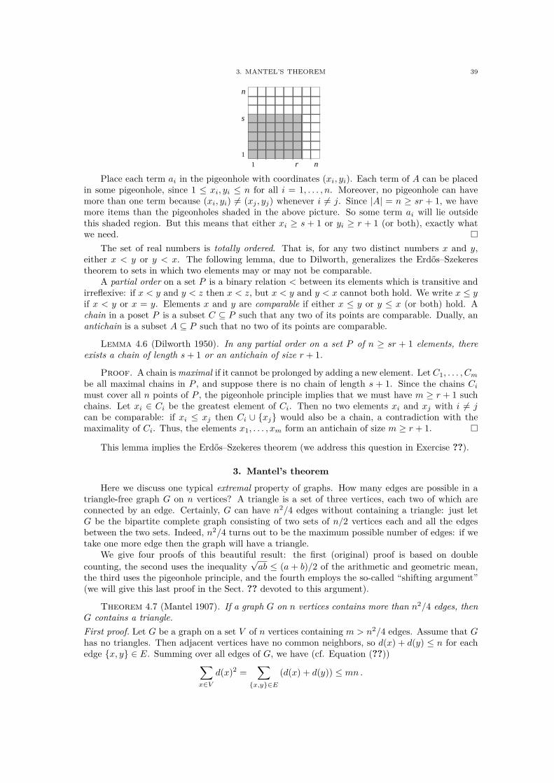
3. MANTEL’S THEOREM 39
r n1
1
s
n
Place each term ai in the pigeonhole with coordinates (xi, yi). Each term of A can be placedin some pigeonhole, since 1 ≤ xi, yi ≤ n for all i = 1, . . . , n. Moreover, no pigeonhole can havemore than one term because (xi, yi) 6= (xj , yj) whenever i 6= j. Since |A| = n ≥ sr + 1, we havemore items than the pigeonholes shaded in the above picture. So some term ai will lie outsidethis shaded region. But this means that either xi ≥ s + 1 or yi ≥ r + 1 (or both), exactly whatwe need.
The set of real numbers is totally ordered. That is, for any two distinct numbers x and y,either x < y or y < x. The following lemma, due to Dilworth, generalizes the Erdős–Szekerestheorem to sets in which two elements may or may not be comparable.
A partial order on a set P is a binary relation < between its elements which is transitive andirreflexive: if x < y and y < z then x < z, but x < y and y < x cannot both hold. We write x ≤ yif x < y or x = y. Elements x and y are comparable if either x ≤ y or y ≤ x (or both) hold. Achain in a poset P is a subset C ⊆ P such that any two of its points are comparable. Dually, anantichain is a subset A ⊆ P such that no two of its points are comparable.
Lemma 4.6 (Dilworth 1950). In any partial order on a set P of n ≥ sr + 1 elements, thereexists a chain of length s + 1 or an antichain of size r + 1.
Proof. A chain is maximal if it cannot be prolonged by adding a new element. Let C1, . . . , Cm
be all maximal chains in P , and suppose there is no chain of length s + 1. Since the chains Ci
must cover all n points of P , the pigeonhole principle implies that we must have m ≥ r + 1 suchchains. Let xi ∈ Ci be the greatest element of Ci. Then no two elements xi and xj with i 6= jcan be comparable: if xi ≤ xj then Ci ∪ xj would also be a chain, a contradiction with themaximality of Ci. Thus, the elements x1, . . . , xm form an antichain of size m ≥ r + 1.
This lemma implies the Erdős–Szekeres theorem (we address this question in Exercise ??).
3. Mantel’s theorem
Here we discuss one typical extremal property of graphs. How many edges are possible in atriangle-free graph G on n vertices? A triangle is a set of three vertices, each two of which areconnected by an edge. Certainly, G can have n2/4 edges without containing a triangle: just letG be the bipartite complete graph consisting of two sets of n/2 vertices each and all the edgesbetween the two sets. Indeed, n2/4 turns out to be the maximum possible number of edges: if wetake one more edge then the graph will have a triangle.
We give four proofs of this beautiful result: the first (original) proof is based on double
counting, the second uses the inequality√
ab ≤ (a + b)/2 of the arithmetic and geometric mean,the third uses the pigeonhole principle, and the fourth employs the so-called “shifting argument”(we will give this last proof in the Sect. ?? devoted to this argument).
Theorem 4.7 (Mantel 1907). If a graph G on n vertices contains more than n2/4 edges, thenG contains a triangle.
First proof. Let G be a graph on a set V of n vertices containing m > n2/4 edges. Assume that Ghas no triangles. Then adjacent vertices have no common neighbors, so d(x) + d(y) ≤ n for eachedge x, y ∈ E. Summing over all edges of G, we have (cf. Equation (??))
∑
x∈V
d(x)2 =∑
x,y∈E
(d(x) + d(y)) ≤ mn .
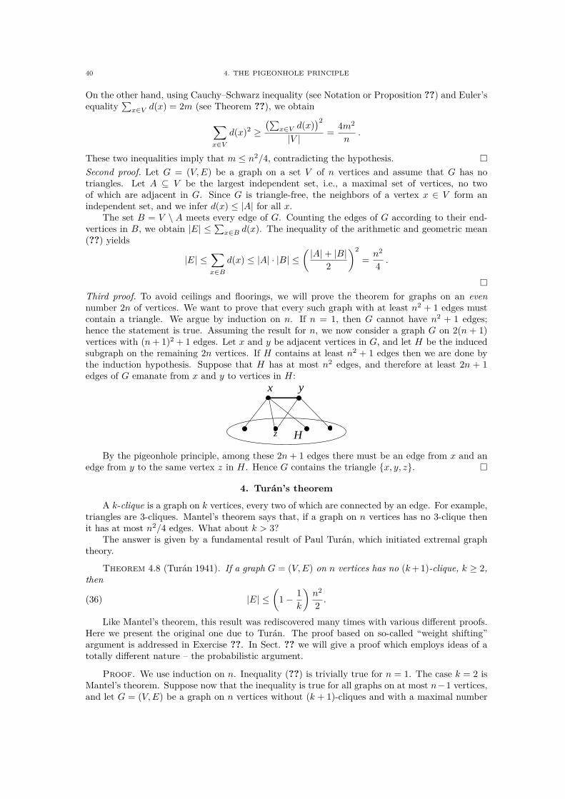
40 4. THE PIGEONHOLE PRINCIPLE
On the other hand, using Cauchy–Schwarz inequality (see Notation or Proposition ??) and Euler’sequality
∑x∈V d(x) = 2m (see Theorem ??), we obtain
∑
x∈V
d(x)2 ≥(∑
x∈V d(x))2
|V | =4m2
n.
These two inequalities imply that m ≤ n2/4, contradicting the hypothesis.
Second proof. Let G = (V, E) be a graph on a set V of n vertices and assume that G has notriangles. Let A ⊆ V be the largest independent set, i.e., a maximal set of vertices, no twoof which are adjacent in G. Since G is triangle-free, the neighbors of a vertex x ∈ V form anindependent set, and we infer d(x) ≤ |A| for all x.
The set B = V \ A meets every edge of G. Counting the edges of G according to their end-vertices in B, we obtain |E| ≤ ∑
x∈B d(x). The inequality of the arithmetic and geometric mean(??) yields
|E| ≤∑
x∈B
d(x) ≤ |A| · |B| ≤( |A| + |B|
2
)2
=n2
4.
Third proof. To avoid ceilings and floorings, we will prove the theorem for graphs on an evennumber 2n of vertices. We want to prove that every such graph with at least n2 + 1 edges mustcontain a triangle. We argue by induction on n. If n = 1, then G cannot have n2 + 1 edges;hence the statement is true. Assuming the result for n, we now consider a graph G on 2(n + 1)vertices with (n + 1)2 + 1 edges. Let x and y be adjacent vertices in G, and let H be the inducedsubgraph on the remaining 2n vertices. If H contains at least n2 + 1 edges then we are done bythe induction hypothesis. Suppose that H has at most n2 edges, and therefore at least 2n + 1edges of G emanate from x and y to vertices in H:
Hz
yx
By the pigeonhole principle, among these 2n + 1 edges there must be an edge from x and anedge from y to the same vertex z in H. Hence G contains the triangle x, y, z.
4. Turán’s theorem
A k-clique is a graph on k vertices, every two of which are connected by an edge. For example,triangles are 3-cliques. Mantel’s theorem says that, if a graph on n vertices has no 3-clique thenit has at most n2/4 edges. What about k > 3?
The answer is given by a fundamental result of Paul Turán, which initiated extremal graphtheory.
Theorem 4.8 (Turán 1941). If a graph G = (V, E) on n vertices has no (k + 1)-clique, k ≥ 2,then
(36) |E| ≤(
1 − 1
k
)n2
2.
Like Mantel’s theorem, this result was rediscovered many times with various different proofs.Here we present the original one due to Turán. The proof based on so-called “weight shifting”argument is addressed in Exercise ??. In Sect. ?? we will give a proof which employs ideas of atotally different nature – the probabilistic argument.
Proof. We use induction on n. Inequality (??) is trivially true for n = 1. The case k = 2 isMantel’s theorem. Suppose now that the inequality is true for all graphs on at most n−1 vertices,and let G = (V, E) be a graph on n vertices without (k + 1)-cliques and with a maximal number
5. DIRICHLET’S THEOREM 41
of edges. This graph certainly contains k-cliques, since otherwise we could add edges. Let A be ak-clique, and set B = V \ A.
Since each two vertices of A are joined by an edge, A contains eA =(
k2
)edges. Let eB be the
number of edges joining the vertices of B and eA,B the number of edges between A and B. Byinduction, we have
eB ≤(
1 − 1
k
)(n − k)2
2.
Since G has no (k + 1)-clique, every x ∈ B is adjacent to at most k − 1 vertices in A, and weobtain
eA,B ≤ (k − 1)(n − k).
Summing up and using the identity
(1 − 1
k
)n2
2=
(k
2
)(n
k
)2
we conclude that
|E| ≤ eA + eB + eA,B ≤(
k
2
)+
(k
2
)(n − k
k
)2
+ (k − 1)(n − k)
=
(k
2
)(1 +
n − k
k
)2
=
(1 − 1
k
)n2
2.
An n-vertex graph T (n, k) that does not contain any (k + 1)-clique may be formed by parti-tioning the set of vertices into k parts of equal or nearly-equal size, and connecting two verticesby an edge whenever they belong to two different parts. Thus, Turán’s theorem states that thegraph T (n, k) has the largest number of edges among all n-vertex graphs without (k + 1)-cliques.
5. Dirichlet’s theorem
Here is the application of the pigeonhole principle which Dirichlet made, resulting in his namebeing attached to the principle. It concerns the existence of good rational approximations toirrational numbers. The result belongs to number theory, but the argument is combinatorial.
Theorem 4.9 (Dirichlet 1879). Let x be a real number. For any natural number n, there is arational number p/q such that 1 ≤ q ≤ n and
∣∣∣∣x − p
q
∣∣∣∣ <1
nq≤ 1
q2 .
Note that it is easy to get an approximation whose error is at most 1/n, by fxing the denom-inator to be q = n. The improved approximation uses the pigeonhole principle.
Proof. For this proof, we let x denote the fractional part of the real number x, that is,x := x − ⌊x⌋. Consider the n + 1 numbers ax, a = 1, 2, . . . , n + 1. We put these numbers intothe n pigeonholes
[0, 1/n) , [1/n, 2/n) , . . . , [1 − 1/n, 1) .
By the pigeonhole principle, some interval contains more than one of the numbers, say ax andbx with a > b, which therefore differ by less than 1/n. Letting q = a−b, we see that there existsan integer p = ⌊ax⌋ − ⌊bx⌋ such that |qx − p| < 1/n, from which the result follows on division byq. Moreover, q is the difference between two integers in the range 1, . . . , n + 1, so q ≤ n.
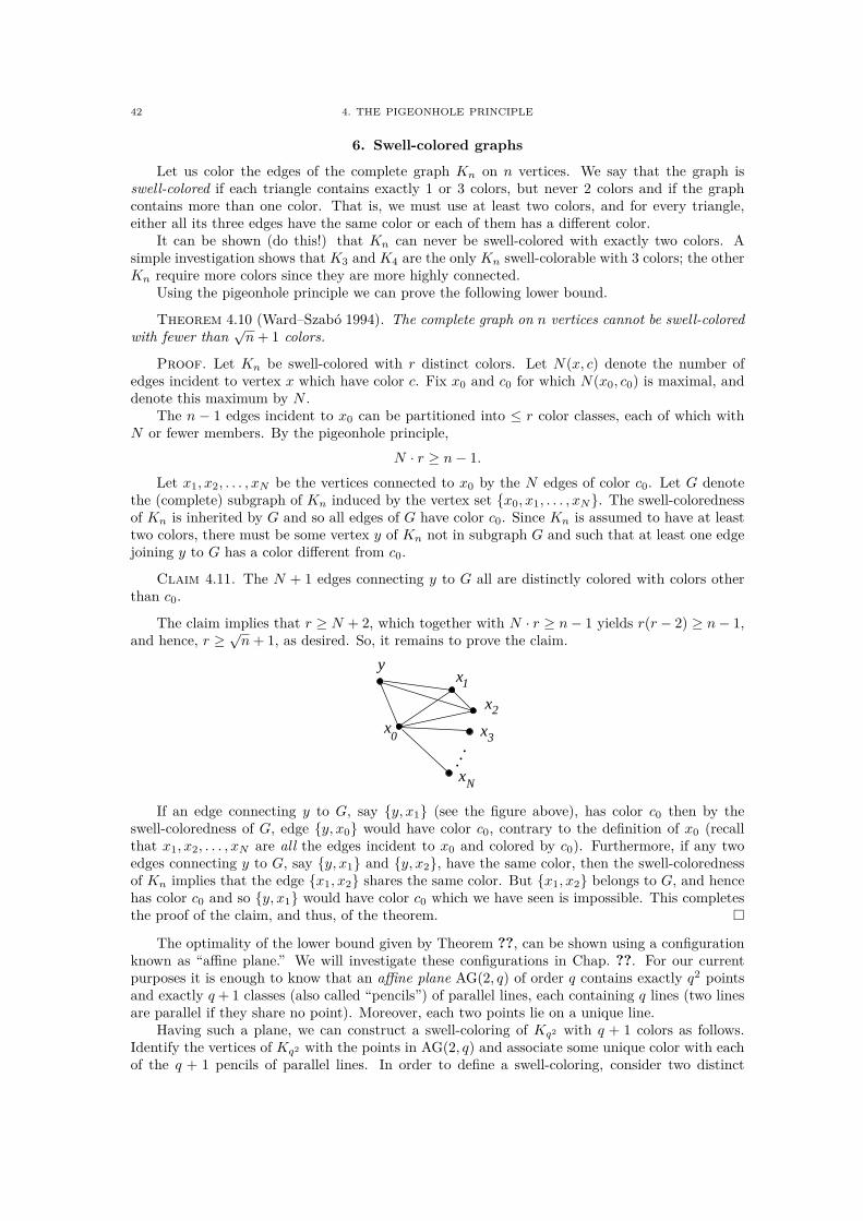
42 4. THE PIGEONHOLE PRINCIPLE
6. Swell-colored graphs
Let us color the edges of the complete graph Kn on n vertices. We say that the graph isswell-colored if each triangle contains exactly 1 or 3 colors, but never 2 colors and if the graphcontains more than one color. That is, we must use at least two colors, and for every triangle,either all its three edges have the same color or each of them has a different color.
It can be shown (do this!) that Kn can never be swell-colored with exactly two colors. Asimple investigation shows that K3 and K4 are the only Kn swell-colorable with 3 colors; the otherKn require more colors since they are more highly connected.
Using the pigeonhole principle we can prove the following lower bound.
Theorem 4.10 (Ward–Szabó 1994). The complete graph on n vertices cannot be swell-coloredwith fewer than
√n + 1 colors.
Proof. Let Kn be swell-colored with r distinct colors. Let N(x, c) denote the number ofedges incident to vertex x which have color c. Fix x0 and c0 for which N(x0, c0) is maximal, anddenote this maximum by N .
The n − 1 edges incident to x0 can be partitioned into ≤ r color classes, each of which withN or fewer members. By the pigeonhole principle,
N · r ≥ n − 1.
Let x1, x2, . . . , xN be the vertices connected to x0 by the N edges of color c0. Let G denotethe (complete) subgraph of Kn induced by the vertex set x0, x1, . . . , xN . The swell-colorednessof Kn is inherited by G and so all edges of G have color c0. Since Kn is assumed to have at leasttwo colors, there must be some vertex y of Kn not in subgraph G and such that at least one edgejoining y to G has a color different from c0.
Claim 4.11. The N + 1 edges connecting y to G all are distinctly colored with colors otherthan c0.
The claim implies that r ≥ N + 2, which together with N · r ≥ n − 1 yields r(r − 2) ≥ n − 1,and hence, r ≥ √
n + 1, as desired. So, it remains to prove the claim.
...
x
x
x
x
x
y1
2
3
N
0
If an edge connecting y to G, say y, x1 (see the figure above), has color c0 then by theswell-coloredness of G, edge y, x0 would have color c0, contrary to the definition of x0 (recallthat x1, x2, . . . , xN are all the edges incident to x0 and colored by c0). Furthermore, if any twoedges connecting y to G, say y, x1 and y, x2, have the same color, then the swell-colorednessof Kn implies that the edge x1, x2 shares the same color. But x1, x2 belongs to G, and hencehas color c0 and so y, x1 would have color c0 which we have seen is impossible. This completesthe proof of the claim, and thus, of the theorem.
The optimality of the lower bound given by Theorem ??, can be shown using a configurationknown as “affine plane.” We will investigate these configurations in Chap. ??. For our currentpurposes it is enough to know that an affine plane AG(2, q) of order q contains exactly q2 pointsand exactly q + 1 classes (also called “pencils”) of parallel lines, each containing q lines (two linesare parallel if they share no point). Moreover, each two points lie on a unique line.
Having such a plane, we can construct a swell-coloring of Kq2 with q + 1 colors as follows.Identify the vertices of Kq2 with the points in AG(2, q) and associate some unique color with eachof the q + 1 pencils of parallel lines. In order to define a swell-coloring, consider two distinct
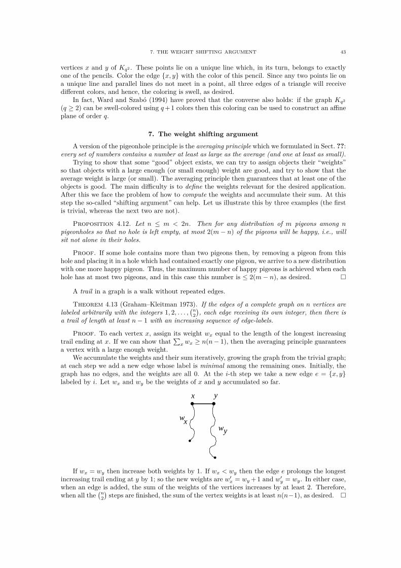
7. THE WEIGHT SHIFTING ARGUMENT 43
vertices x and y of Kq2 . These points lie on a unique line which, in its turn, belongs to exactlyone of the pencils. Color the edge x, y with the color of this pencil. Since any two points lie ona unique line and parallel lines do not meet in a point, all three edges of a triangle will receivedifferent colors, and hence, the coloring is swell, as desired.
In fact, Ward and Szabó (1994) have proved that the converse also holds: if the graph Kq2
(q ≥ 2) can be swell-colored using q +1 colors then this coloring can be used to construct an affineplane of order q.
7. The weight shifting argument
A version of the pigeonhole principle is the averaging principle which we formulated in Sect. ??:every set of numbers contains a number at least as large as the average (and one at least as small).
Trying to show that some “good” object exists, we can try to assign objects their “weights”so that objects with a large enough (or small enough) weight are good, and try to show that theaverage weight is large (or small). The averaging principle then guarantees that at least one of theobjects is good. The main difficulty is to define the weights relevant for the desired application.After this we face the problem of how to compute the weights and accumulate their sum. At thisstep the so-called “shifting argument” can help. Let us illustrate this by three examples (the firstis trivial, whereas the next two are not).
Proposition 4.12. Let n ≤ m < 2n. Then for any distribution of m pigeons among npigeonholes so that no hole is left empty, at most 2(m − n) of the pigeons will be happy, i.e., willsit not alone in their holes.
Proof. If some hole contains more than two pigeons then, by removing a pigeon from thishole and placing it in a hole which had contained exactly one pigeon, we arrive to a new distributionwith one more happy pigeon. Thus, the maximum number of happy pigeons is achieved when eachhole has at most two pigeons, and in this case this number is ≤ 2(m − n), as desired.
A trail in a graph is a walk without repeated edges.
Theorem 4.13 (Graham–Kleitman 1973). If the edges of a complete graph on n vertices arelabeled arbitrarily with the integers 1, 2, . . . ,
(n2
), each edge receiving its own integer, then there is
a trail of length at least n − 1 with an increasing sequence of edge-labels.
Proof. To each vertex x, assign its weight wx equal to the length of the longest increasingtrail ending at x. If we can show that
∑x wx ≥ n(n − 1), then the averaging principle guarantees
a vertex with a large enough weight.We accumulate the weights and their sum iteratively, growing the graph from the trivial graph;
at each step we add a new edge whose label is minimal among the remaining ones. Initially, thegraph has no edges, and the weights are all 0. At the i-th step we take a new edge e = x, ylabeled by i. Let wx and wy be the weights of x and y accumulated so far.
x
x y
wy
w
If wx = wy then increase both weights by 1. If wx < wy then the edge e prolongs the longestincreasing trail ending at y by 1; so the new weights are w′
x = wy + 1 and w′y = wy. In either case,
when an edge is added, the sum of the weights of the vertices increases by at least 2. Therefore,when all the
(n2
)steps are finished, the sum of the vertex weights is at least n(n−1), as desired.
44 4. THE PIGEONHOLE PRINCIPLE
Finally, we illustrate the shifting argument by the fourth proof of Mantel’s theorem: If a graphG on 2n vertices contains n2 + 1 edges, then G contains a triangle.
Fourth proof of Mantel’s theorem (Motzkin–Straus 1965). Let G be a graph on 2n vertices, andlet m be the number of edges in G. Assume that G has no triangles. Our goal is to prove thatthen m ≤ n2. We assign a nonnegative wx to each vertex x such that
∑x wx = 1. We seek to
maximizeS :=
∑wxwy,
where the sum is taken over all edges x, y of G. One way of assigning the weights is to letwx = 1/(2n) for each x. This gives
(37) S ≥ m
(2n)2 .
We are going to show that, on the other hand, S never exceeds 1/4, which together with theprevious lower bound will imply that m ≤ n2, as desired.
And now comes the “shifting argument.” Suppose that x and y are two nonadjacent verticesand Wx and Wy are the total weights of vertices connected to x and y, respectively. Suppose alsothat Wx ≥ Wy. Then for any ǫ ≥ 0,
(wx + ǫ)Wx + (wy − ǫ)Wy ≥ wxWx + wyWy.
This, in particular, means that we do not decrease the value of S if we shift all of the weight ofvertex y to the vertex x. It follows that S is maximized when all of the weight is concentratedon a complete subgraph of G. But we have assumed that G has no triangles; so G cannot havecomplete subgraphs other than single edges. Hence, S is maximized when all of the weight isconcentrated on two adjacent vertices, say x and y. Therefore
S ≤ max
wx · wy : wx + wy = 1
= 1/4
which, together with (??), yield the desired upper bound m ≤ n2.
8. Schur’s theorem
The famous Fermat’s Last Theorem states that if n > 2, then xn + yn = zn has no solutionsin nonzero integers x, y and z. This theorem was first conjectured by Pierre de Fermat in 1637,but was not proven until 1995 despite the efforts of many mathematicians. The last step in itsproof was done by Andrew Wiles.
As early as 1916, Issai Schur used the pigeonhole principle to show that Fermat’s Last Theoremis false in the finite field Zp for any sufficiently large prime p. He derived this from the followingcombinatorial result about colorings of numbers. The result may perhaps be considered as theearliest result in Ramsey theory.
An r-coloring of a set assigns one of the colors 1, 2, . . . , r to each element of the set.
Theorem 4.14 (Schur 1916). For any r ≥ 2 and for any r-coloring of 1, 2, . . . , n, wheren = ⌈er!⌉, there are three integers x, y, z of the same color and such that x + y = z.
Proof. Let χ : 1, . . . , n → 1, . . . , r be an r-coloring of the first n positive integers.Assume that there do not exist positive integers x, y with x + y ≤ n such that χ(x) = χ(y) =χ(x + y). Our goal is to show that then n < er!.
Let c0 be a color which appears most frequently among the n elements, and let x0 < x1 <. . . < xn1−1 be the elements of color c0. By the pigeonhole principle, we know that n ≤ rn1,
Consider the set A0 = xi − x0 : 1 ≤ i < n1. By our assumption, no number in A0 canreceive color c0. So, the set A0 is colored by r − 1 colors. Let c1 be a color which appears mostfrequently among the elements of A0, and let y0 < y1 < . . . < yn2−1 be its elements of color c1.Observe that n1 − 1 ≤ (r − 1)n2.
Consider the set A1 = yi − y0 : 1 ≤ i < n2. By the assumption, no number in A1 canreceive any of colors c0 and c1. So, the set A1 is colored by r − 2 colors. Let c2 be a color whichappears most frequently among the elements of A1, and let z0 < z1 < . . . < zn3−1 be its elementsof color c2. Observe that n2 − 1 ≤ (r − 2)n3.

9. RAMSEYAN THEOREMS FOR GRAPHS 45
e
Figure 2. What is the color of e?
Continue this procedure until some nk becomes 1. Since we have only r colors, this happensat the latest for k = r. Thus, we obtained the inequalities n ≤ rn1 and ni ≤ (r − i)ni+1 + 1 fori = 1, . . . , k − 1, with nk = 1. Putting them together we obtain that
n ≤r−1∑
i=0
r(r − 1)(r − 2) · · · (r − i) =r−1∑
i=0
r!
i!< r!
∞∑
i=0
1
i!= er!
Schur (1916) used Theorem ?? to show that Fermat’s Last Theorem is false in the finite fieldZp for any sufficiently large prime p.
Theorem 4.15. For every integer n ≥ 1, there exists p0 such that for any prime p ≥ p0, thecongruence
xn + yn = zn mod p
has a solution.
Proof. The multiplicative group Z∗p = 1, 2, . . . , p − 1 is known to be cyclic and hence it
has a generator g. Each element of Z∗p can be written as x = gnj+i where 0 ≤ i < n. We color
the elements of Z∗p by n colors, where χ(x) = i if x = gnj+i. By Schur’s theorem, for p sufficiently
large, there are elements x′, y′, z′ ∈ Z∗p such that x′ +y′ = z′ and χ(x′) = χ(y′) = χ(z′). Therefore,
x′ = gnjx+i, y′ = gnjy+i, z′ = gnjz+i and
gnjx+i + gnjy+i = gnjz+i .
Setting x = gjx , y = gjy and z = gjz , we get a solution of xn + yn = zn in Z∗p.
9. Ramseyan theorems for graphs
How many people can we invite to a party where among each three people there are two whoknow each other and two who don’t know each other? It turns out that at most five persons canattend such a party.
To show this, let us consider the following simple game. Mark six points on the paper, nothree in line. There are two players; one has a Red pencil the other Blue. Each player’s turnconsists in drawing a line with his/her pencil between two of the points which haven’t alreadybeen joined. (The crossing of lines is allowed). The player’s goal is to create a triangle in his/hercolor. If you try to play it with a friend, you will notice that it always end in a win for one player:a draw is not possible. Prove this! (Hint: see Fig. ??.)
We can generalize this argument to arbitrary graphs, not only those with up to six vertices.Let G = (V, E) be an undirected graph. A subset S ⊆ V is a clique of G if any two vertices
of S are adjacent. Similarly, a subset T ⊆ V is an independent set of G if no two vertices of T areadjacent in G.
For integers s, t ≥ 1, let R(s, t) denote the smallest number n such that in any(!) graph on nor more vertices, there exists either a clique of s vertices or an independent set of t vertices.
Theorem 4.16.
R(s, t) ≤(
s + t − 2
s − 1
)=
(s + t − 2
t − 1
).
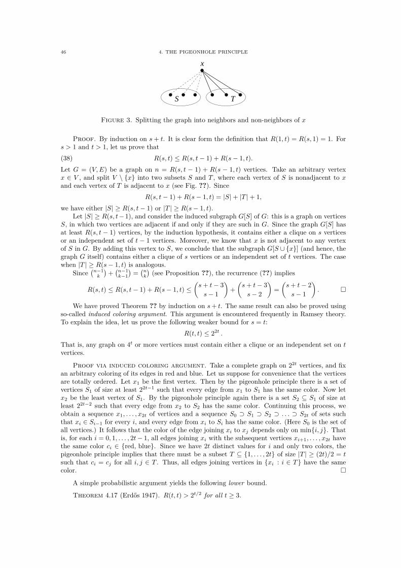
46 4. THE PIGEONHOLE PRINCIPLE
S T
x
Figure 3. Splitting the graph into neighbors and non-neighbors of x
Proof. By induction on s + t. It is clear form the definition that R(1, t) = R(s, 1) = 1. Fors > 1 and t > 1, let us prove that
(38) R(s, t) ≤ R(s, t − 1) + R(s − 1, t).
Let G = (V, E) be a graph on n = R(s, t − 1) + R(s − 1, t) vertices. Take an arbitrary vertexx ∈ V , and split V \ x into two subsets S and T , where each vertex of S is nonadjacent to xand each vertex of T is adjacent to x (see Fig. ??). Since
R(s, t − 1) + R(s − 1, t) = |S| + |T | + 1,
we have either |S| ≥ R(s, t − 1) or |T | ≥ R(s − 1, t).Let |S| ≥ R(s, t−1), and consider the induced subgraph G[S] of G: this is a graph on vertices
S, in which two vertices are adjacent if and only if they are such in G. Since the graph G[S] hasat least R(s, t − 1) vertices, by the induction hypothesis, it contains either a clique on s verticesor an independent set of t − 1 vertices. Moreover, we know that x is not adjacent to any vertexof S in G. By adding this vertex to S, we conclude that the subgraph G[S ∪ x] (and hence, thegraph G itself) contains either a clique of s vertices or an independent set of t vertices. The casewhen |T | ≥ R(s − 1, t) is analogous.
Since(
n−1k
)+(
n−1k−1
)=(
nk
)(see Proposition ??), the recurrence (??) implies
R(s, t) ≤ R(s, t − 1) + R(s − 1, t) ≤(
s + t − 3
s − 1
)+
(s + t − 3
s − 2
)=
(s + t − 2
s − 1
).
We have proved Theorem ?? by induction on s + t. The same result can also be proved usingso-called induced coloring argument. This argument is encountered frequently in Ramsey theory.To explain the idea, let us prove the following weaker bound for s = t:
R(t, t) ≤ 22t .
That is, any graph on 4t or more vertices must contain either a clique or an independent set on tvertices.
Proof via induced coloring argument. Take a complete graph on 22t vertices, and fixan arbitrary coloring of its edges in red and blue. Let us suppose for convenience that the verticesare totally ordered. Let x1 be the first vertex. Then by the pigeonhole principle there is a set ofvertices S1 of size at least 22t−1 such that every edge from x1 to S1 has the same color. Now letx2 be the least vertex of S1. By the pigeonhole principle again there is a set S2 ⊆ S1 of size atleast 22t−2 such that every edge from x2 to S2 has the same color. Continuing this process, weobtain a sequence x1, . . . , x2t of vertices and a sequence S0 ⊃ S1 ⊃ S2 ⊃ . . . ⊃ S2t of sets suchthat xi ∈ Si−1 for every i, and every edge from xi to Si has the same color. (Here S0 is the set ofall vertices.) It follows that the color of the edge joining xi to xj depends only on mini, j. Thatis, for each i = 0, 1, . . . , 2t − 1, all edges joining xi with the subsequent vertices xi+1, . . . , x2t havethe same color ci ∈ red, blue. Since we have 2t distinct values for i and only two colors, thepigeonhole principle implies that there must be a subset T ⊆ 1, . . . , 2t of size |T | ≥ (2t)/2 = tsuch that ci = cj for all i, j ∈ T . Thus, all edges joining vertices in xi : i ∈ T have the samecolor.
A simple probabilistic argument yields the following lower bound.
Theorem 4.17 (Erdős 1947). R(t, t) > 2t/2 for all t ≥ 3.

10. RAMSEY’S THEOREM FOR SETS 47
That is, the edges of Kn can be colored in two colors so that we get no monochromatic K2 log n.
Proof. Consider a random 2-coloring of the edges of Kn obtained by coloring each edgeindependently either red or blue, where each color is equally likely. For any fixed set T of tvertices, the probability that all
(t2
)edges between these vertices receive the same color (i.e., that
either all edges are red or they are blue) is 2 · 2−(t2). The number of t-element subsets of vertices(
nt
)and therefore the probability that there is at least one monochromatic t-clique is at most
(n
t
)· 21−(t
2) <nt
t!· 21+t/2
2t2/2,
which is < 1 if n ≤ 2t/2 and t ≥ 3.
Using Stirling’s Formula, the lower bound on R(t, t) can be improved to about t2t/2. On theother hand, Theorem ?? gives an upper bound
(2tt
)on R(t + 1, t + 1). This bound was recently
improved by Conlon (2009) to about t−ℓ(2t
t
)with ℓ ≥ c log n/ log log n. The gap is still large, and
tight bounds are known only for s = 3:
c1t2
log t≤ R(3, t) ≤ c2
t2
log t.
The upper bound is due to Ajtai, Komlós, and Szemerédi (1980) and the lower bound was provedby Kim (1995) using a probabilistic argument.
In the case of bipartite graphs the following bounds are known. Let b(t) be the smallestnumber n such that, in any two-coloring of the complete bipartite n × n graph Kn,n there is a
monochromatic Kt,t. The best known lower bound b(t) = Ω(k2k/2) is the same as for ordinarygraphs. The best known upper bound b(t) = O(2k log k) was proved by Conlon (2008).
10. Ramsey’s theorem for sets
We now consider colorings of k-element subsets of [n] for k > 2. The Ramsey theorem forgraphs (we just proved) speaks about the case k = 2: for every s ≥ 1, there is an n such that itis not possible to color 2-element subsets of [n] (edges) in red and blue so that every s-elementsubset of [n] will contain two 2-element subsets of different colors. (In this case n ≥ 4s is enough.)In its unabridged form, the celebrated result of Ramsey (1930) speaks about colorings of largersubsets using any number of colors.
Theorem 4.18 (Ramsey’s theorem). For every natural numbers 1 ≤ k ≤ s and r ≥ 2 thereexists a natural number n = Rr(k; s) such that whenever k-subsets of [n] are colored in r colors,there is an s-subset of [n] whose all k-subsets receive the same color.
Proof. We first observe that it is enough to consider the case of r = 2 colors.
Claim 4.19. Rr+1(k; s) ≤ Rr (k; R2(k; s)).
Proof. Let N = Rr (k; R2(k; s)) and let an arbitrary coloring of k-subsets of an N -elementset X with r+1 colors 0, 1, . . . , r be given. Then consider this as an r-coloring simply by identifyingthe colors 0 and 1. (This is known as the “mixing colors” trick.) By the choice of N , either thereexists an R2(k; s)-element subset, all whose k-subsets receive one of the colors 2, . . . , r (and weare done), or there exists an R2(k; s)-element subset Y with each its k-subsets in color 0 or 1.According to the size of Y , all k-subsets of some its s-element subset must be monochromatic.
By Claim ??, it is enough to show that R2(k; s) exists.In order to argue by induction, we define a more “granulated” version of the Ramsey number
R2(k; s). Namely let R(k; s, t) be the smallest number n with the following property: If k-subsetsof an n-set are colored with two colors 0 and 1, then all k-subsets of some s-subset receive color0 or all k-subsets of some t-subset receive color 1. Thus, the theorem claims that R(k; s, s) existsfor all s ≥ k. We will prove a stronger statement that R(k; s, t) ≤ n, where
n := R (k − 1; R(k; s − 1, t), R(k; s, t − 1)) + 1.

48 4. THE PIGEONHOLE PRINCIPLE
d
a
b
c
Figure 4. Point d lies in none of the lines ab, bc and ac.
We prove this recurrence by induction on k and on s, t. Observe that, by the pigeonhole principle,R(1; s, t) = s + t − 1 for all s and t and, moreover, R(k; x, k) = R(k; k, x) = x for all k and x ≥ k.By induction, we may assume that the numbers R(k; s − 1, t) and R(k; s, t − 1) exist, and take anarbitrary n-element set X, where n is defined above.
Let χ be a coloring of k-subsets of X with two colors 0 and 1. Fix a point x ∈ X, and letX ′ := X \ x. We define a new coloring χ′ of the (k − 1)-subsets A of X ′ by
χ′(A) := χ (A ∪ x) .
By the choice of n and by symmetry, we can assume to have found a subset Y ⊆ X ′ such that|Y | = R(k; s − 1, t) and
χ′(A) = 0 for all (k − 1)-subsets A of Y .
Now consider how the original coloring χ acts on the k-subsets of Y . According to its size, the setY must either contain a t-element subset, all whose k-subsets receive color 1 (and we are done),or it must contain an (s − 1)-element subset Z, all whose k-subsets receive color 0. In this lastcase consider the s-element subset Z ∪ x and take an arbitrary its subset B of size k. If x 6∈ Bthen B is a k-element subset of Z, and hence, χ(B) = 0. If x ∈ B then the set A = B \ x is a(k − 1)-subset of Y , and hence again, χ(B) = χ (A ∪ x) = χ′(A) = 0.
One of the earliest and most popular applications of Ramsey’s theorem is due to Erdős andSzekeres (1935). In fact, this application was a first step in popularizing Ramsey’s theorem.
Theorem 4.20 (Erdős–Szekeres 1935). Let m ≥ 3 be a positive integer. Then there existsa positive integer n such that any set of n points in the Euclidean plane, no three of which arecollinear, contains m points which are the vertices of a convex m-gon.
Proof (due to Johnson 1986). Choose n = R2(3; m), the number from the Ramsey’s Theorem ??,and let A be any set of n points in the plane, no three of which are collinear (i.e., lie on a line).For a, b, c ∈ A, let |abc| denote the number of points of A which lie in the interior of the trianglespanned by a, b and c. Define the 2-coloring χ of triples of points in A by χ(a, b, c) = 0 if |abc| iseven and χ(a, b, c) = 1 otherwise. By the choice of n, there exists an m-element subset B ⊆ A suchthat all its 3-element subsets receive the same color. Then the points of B form a convex m-gon.Otherwise, there would be four points a, b, c, d ∈ B such that d lies in the interior of the triangleabc (see Fig. ??). Since no three points of B are collinear, we have |abc| = |abd|+ |acd|+ |bcd|+1,contradicting that the coloring χ is constant on all triples from B.
Exercises
Ex 4.1. Suppose five points are chosen inside an equilateral triangle with side-length 1. Showthat there is at least one pair of points whose distance apart is at most 1/2. Hint: Divide thetriangle into four suitable boxes.
Ex 4.2. (D.R. Karger). Jellybeans of 8 different colors are in 6 jars. There are 20 jellybeansof each color. Use the pigeonhole principle to prove that there must be a jar containing two pairsof jellybeans from two different colors of jellybeans. Hint: For each color there is a jar containing apair of jellybeans of that color, and we have more colors than jars.

EXERCISES 49
Ex 4.3. Show that for any positive integer n, there is a multiple of n that contains only thedigits 7 or 0. Hint: Consider the values modulo n of all the numbers ai of the form 77 . . . 7, with i sevens,i = 1, . . . , n + 1.
Ex 4.4. Prove that every set of n + 1 distinct integers chosen from 1, 2, . . . , 2n contains apair of consecutive numbers and a pair whose sum is 2n + 1. For each n, exhibit two sets of size nto show that these results are the best possible. Hint: Use pigeonholes (2i, 2i − 1) and (i, 2n − i + 1),i = 1, . . . , n.
Ex 4.5. Prove that every set of n + 1 distinct integers chosen from 1, 2, . . . , 2n contains twonumbers such that one divides the other. Sketch: (due to Lajos Pósa): Write every number x in theform x = kx2a, where kx is an odd number between 1 and 2n − 1. Take odd pigeonholes 1, 3, 5, . . . , 2n − 1and put x into the pigeonhole number kx. Some hole must have two numbers x < y.
Ex 4.6. Coin-weighing problem (Erdős–Spencer 1974). Let n coins of weights 0 and 1 be given.We are also given a scale with which we may weigh any subset of the coins. The information fromprevious weighings may be used. The object is to determine the weights of the coins with theminimal number of weighings. Formally, the problem may be stated as follows. A collectionS1, . . . , Sm of subsets of [n] is called determining if an arbitrary subset T of [n] can be uniquelydetermined by the cardinalities |Si ∩T |, 1 ≤ i ≤ m. Let D(n) be the minimum m for which such adetermining collection exists. By weighting each coin separately (Si = i) we see that D(n) ≤ n.Show that D(n) ≥ n/ (log2(n + 1)). Hint: Take a determining collection S1, . . . , Sm, observe that foreach i there are only n + 1 possible |Si ∩ T |, and apply the pigeonhole principle.
Ex 4.7. Suppose that n is a multiple of k. Construct a graph without (k + 1)-cliques, inwhich the number of edges achieves the upper bound (??) given by Turán’s theorem. Hint: Splitthe n vertices into k equal size parts and join all pairs of vertices from different parts (this is a completek-partite graph).
Ex 4.8. Recall that the independence number α(G) of a graph G is the maximum number ofpairwise nonadjacent vertices of G. Prove the following dual version of Turán’s theorem: if G is agraph with n vertices and nk/2 edges, k ≥ 1, then α(G) ≥ n/(k + 1).
Ex 4.9. (Motzkin–Straus 1965). Prove Turán’s theorem using the shifting argument describedin the fourth proof of Mantel’s theorem. Hint: Let G be a graph with n vertices and m edges, andsuppose that G has no (k + 1)-clique. Assign weights wx to the vertices as before. Setting wx = 1/n forall vertices, we obtain S ≥ m/n2. On the other hand, the same shifting argument yields that the weightis concentrated on some clique U with |U | = t ≤ k vertices. Setting wx = 1/t for x ∈ U , and wx = 0otherwise, the total weight becomes
(t2
)/t2 = (1 − 1/t)/2. Since this expression is increasing in t, the best
we can do is to set t = k.
Ex 4.10. Derive the Erdős–Szekeres theorem from Lemma ??. Hint: Given a sequence A =(a1, . . . , an) of n ≥ rs + 1 real numbers, define a partial order 4 on A by ai 4 aj if ai ≤ aj and i ≤ j,and apply Dilworth’s lemma.
Ex 4.11. Let n2 + 1 points be given in R2. Prove that there is a sequence of n + 1 points(x1, y1), . . . , (xn+1, yn+1) for which x1 ≤ x2 ≤ · · · ≤ xn+1 and y1 ≥ y2 ≥ · · · ≥ yn+1, or a sequenceof n + 1 points for which x1 ≤ x2 ≤ · · · ≤ xn+1 and y1 ≤ y2 ≤ · · · ≤ yn+1.
Ex 4.12. Show that, if n > srp, then any sequence of n real numbers must contain eithera strictly increasing subsequence of length greater than s, a strictly decreasing subsequence oflength greater than r, or a constant subsequence of length greater than p. Hint: By the pigeonholeprinciple, if only sr or fewer distinct values occur, then some value must be taken by more than p numbersin the sequence. Otherwise, we can argue as in the Erdős–Szekeres theorem.
Ex 4.13. Let 0 < a1 < a2 < · · · < asr+1 be sr + 1 integers. Prove that we can select eithers + 1 of them, no one of which divides any other, or r + 1 of them, each dividing the following one.Hint: Apply Dilworth’s lemma.
50 4. THE PIGEONHOLE PRINCIPLE
Ex 4.14. Show that the bound in the Erdős–Szekeres’ theorem is best possible. Hint: Considerthe sequence A = (Bs−1, Bs−2, . . . , B0), where
Bi = (ir + 1, ir + 2, . . . , ir + r).
Ex 4.15. Use the pigeonhole principle to prove the following fact, known as Chinese remaindertheorem. Let a1, . . . , ak, b be integers, and m = m1 · · · mk where mi and mj are relatively prime,for all i 6= j. Then there exists exactly one integer a, b ≤ a < b + m, such that a ≡ ai mod mi
for all i = 1, . . . , k. Hint: The integers x ∈ b, b + 1, . . . b + m − 1 are different modulo m; hence theirresidues (x mod m1, . . . , x mod mk) run through all m possible values.
Ex 4.16. (Moon–Moser 1962). Let G = (V, E) be a graph on n vertices and t(G) the numberof triangles in it. Show that
t(G) ≥ |E|3n
(4 · |E| − n2) .
Hint: For an edge e = x, y, let t(e) be the number of triangles containing e. Let B = V \ x, y. Amongthe vertices in B there are precisely t(e) vertices which are adjacent to both x and y. Every other vertexin B is adjacent to at most one of these two vertices. We thus obtain d(x) + d(y) − t(e) ≤ n. Summingover all edges e = x, y we obtain
∑
e∈E
(d(x) + d(y)) −∑
e∈E
t(e) ≤ n · |E|.
Apply the Cauchy–Schwarz inequality to estimate the first sum.
Comment: This implies that a graph G on an even number n of vertices with |E| = n2/4 + 1 edges notonly contains one triangle (as it must be by Mantel’s theorem), but more than n/3.
Ex 4.17. (Goodman 1959). Let G be a graph with n vertices and m edges. Let t(G) denotethe number of triangles contained in the graph G or in its complement. Prove that
t(G) ≥(
n
3
)+
2m2
n− m(n − 1).
Hint: Let ti be the number of triples of vertices i, j, k such that the vertex i is adjacent to precisely oneof j or k. Observe that t(G) ≥
(n3
)− 1
2
∑iti and that ti = di(n − 1 − di), where di is the degree of the
vertex i in G. Use the Cauchy–Schwarz inequality (??) and Euler’s theorem (Theorem ??) to show that∑d2
i ≥ 1n
(∑di
)2= 4m2
n.
Ex 4.18. A set S ⊆ V of vertices in a graph G = (V, E) spans an edge e ∈ E if both endpointsof e belong to S. Say that a graph is (k, r)-sparse if every subset of k vertices spans at most r ofits edges. Turán’s theorem (Theorem ??) gives an upper bound on the maximal possible number
of edges in a (k, r)-sparse graph for r =(
k2
)− 1. Show that every (k, r)-sparse graph on n vertices
has at most α ·(
n2
)edges, where α = r ·
(k2
)−1. Hint: Observe that every edge is spanned by precisely(
n−2k−2
)of k-element subsets and use Exercise ??.
Ex 4.19. Color all non-empty subsets (not the points!) of [n] = 1, . . . , n with r colors. Provethat, if n is large enough, then there are two disjoint non-empty subsets A, B such that A, B andA ∪ B have the same color. Hint: Take n = Rr(2; 3). Assume the non-empty subsets of [n] are coloredwith r colors. Now color each pair i, j (1 ≤ i < j ≤ n) by the color of the interval i, i + 1, . . . , j − 1.By Theorem ??, there exists a monochromatic triangle x < y < z. Take A = x, x + 1, . . . , y − 1 andB = y, y + 1, . . . , z − 1.
Ex 4.20. Show that for every r ≥ 2 there exists a constant c = c(r) such that, if n is largeenough, then for every r-coloring of the points 1, . . . , n, at least c · n2 of the pairs i, j of pointswill receive the same color. Hint: By the pigeonhole principle, every (r + 1)-subset of points contributesat least one monochromatic pair, and every pair is contained only in
(n−2r−1
)of such subsets.
Ex 4.21. Prove that R(3, 4) ≤ 9. Hint: Color the edges of K9 in red and blue, and assume thatthere are no red triangles and no blue 4-cliques. Then each vertex is incident to precisely three red edgesand five blue edges. Thus, there are exactly (9 · 3)/2 many red edges. But this should be an integer!

EXERCISES 51
Ex 4.22. Derive the following weaker version of Schur’s theorem (Theorem ??) from Ramsey’stheorem (Theorem ??): For any r ≥ 2 there is n > 3 such that for any r-coloring of 1, 2, . . . , n,there are three integers of the same color and such that x + y = z. Hint: Choose n = Rr(2; 3).Given a coloring χ : [n] → [r] of the points in [n], consider the coloring χ′ of the pairs defined by:χ′(x, y) = χ(|x − y|) What does it means to have a χ′-monochromatic triangle with vertices x < y < z?
Ex 4.23. Use the previous exercise to show that R(4, 4) ≤ 18. Hint: (??).
The next exercises are about the chromatic number χ(G) of graphs. Recall that this is thesmallest number of colors we need in order to color the vertices of G in such a way that no twoadjacent vertices receive the same color.
Ex 4.24. Show that any graph G must have at least(
χ(G)2
)edges.
Ex 4.25. Let G1, G2 be two graphs. Prove that χ(G1 ∪ G2) ≤ χ(G1) · χ(G2). Hint: Use pairsof colors to color G1 ∪ G2.
Ex 4.26. Let G be a graph on n vertices. A complement G of a graph G is a graph on thesame set of vertices in which two vertices are adjacent if and only if they are non-adjacent in G.Prove that χ(G) · χ(G) ≥ n and χ(G) + χ(G) ≥ 2
√n. Hint: (χ(G) − χ(G))2 ≥ 0.
Ex 4.27. Prove that χ(G) ≤ ∆(G) + 1, where ∆(G) is the maximum degree of a vertex in G.Hint: Order the vertices v1, . . . , vn and use greedy coloring: assign to vi the smallest-indexed color notalready used on its lower-indexed neighbors.
Ex 4.28. (Welsh–Powell 1967). Let G be a graph on n vertices, whose degrees are d1 ≥ d2 ≥. . . ≥ dn. Prove that χ(G) ≤ 1 + maxi mindi, i − 1. Hint: Apply the greedy algorithm from theprevious exercise. When we color the i-th vertex, at most mindi, i−1 of its neighbors have already beencolored, so its color is at most 1 + mindi, i − 1.
Ex 4.29. Let G = (V, E) be a graph and S ⊆ V a subset of its vertices. The induced subgraphof G is the graph G[S] on vertices S, in which two vertices are adjacent if and only if they aresuch in the original graph G. Prove that for any graph G we can find a partition V = S ∪ T of itsvertices into two disjoint non-empty subsets S and T such that χ(G[S]) + χ(G[T ]) = χ(G).
Ex 4.30. A graph G is k-critical if χ(G) = k but χ(H) < k for every proper subgraph H ofG. Let δ(G) denote the minimum degree of a vertex in G. Prove the following: if G is a k-criticalgraph, then δ(G) ≥ k − 1. Hint: Assume there is a vertex x ∈ V of degree at most k − 2, and considerthe induced subgraph H = G[V \ x]. Graph H must have a legal (k − 1)-coloring, and at least one ofthese k − 1 colors is not used to color the neighbors of x; we can use it for x.
Ex 4.31. (Szekeres–Wilf 1968). Prove that χ(G) ≤ 1 + maxH⊆G δ(H) holds for any graph G.Hint: Let k = χ(G), take a k-critical subgraph H of G and use the previous estimate.
Ex 4.32. Let G be a directed graph without cycles and suppose that G has no path of lengthk. Prove that then χ(G) ≤ k. Hint: Let c(x) denote the maximum length of a path starting from x.Then c is a coloration with colors 0, 1, . . . , k − 1. Show that it is legal.
Ex 4.33. Let G be a graph on n vertices, and α(G) be its independence number, i.e., themaximal number of vertices, no two of which are joined by an edge. Show that n/α(G) ≤ χ(G) ≤n − α(G) + 1.
Ex 4.34. It is clear that χ(G) ≥ ω(G), where ω(G) is the clique number of G, i.e., themaximum size of a clique in G. Erdős (1947) has proved that, for every large enough n, thereexists an n-vertex graph G such that ω(G) ≤ 2 log2 n and ω(G) ≤ 2 log2 n (see Theorem ?? fora proof). Use this result to show that the gap between χ(G) and ω(G) can be quite large: themaximum of χ(G)/ω(G) over all n-vertex graphs G is Ω
(n/(log2 n)2
). Hint: χ(G) ≥ n/ω(G).
Ex 4.35. Let G = (V, E) be a graph, and (Cv)v∈V be a sequence of (not necessarily disjoint)sets. We can look at each set Cv as a color set (or a “palette”) for the vertex v. Given such alist of color sets, we consider only colorings c such that c(v) ∈ Cv for all v ∈ V , and call them
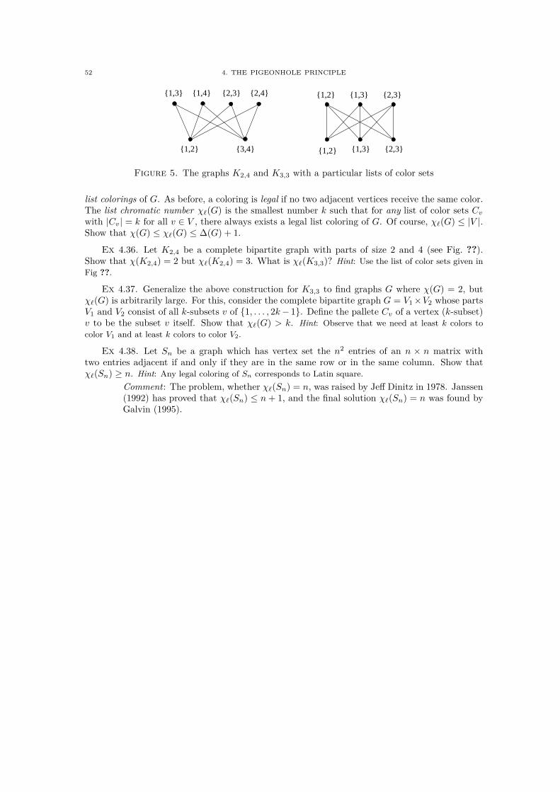
52 4. THE PIGEONHOLE PRINCIPLE
1,2 3,4
2,42,31,41,3
1,2 1,3 2,3
2,31,31,2
Figure 5. The graphs K2,4 and K3,3 with a particular lists of color sets
list colorings of G. As before, a coloring is legal if no two adjacent vertices receive the same color.The list chromatic number χℓ(G) is the smallest number k such that for any list of color sets Cv
with |Cv| = k for all v ∈ V , there always exists a legal list coloring of G. Of course, χℓ(G) ≤ |V |.Show that χ(G) ≤ χℓ(G) ≤ ∆(G) + 1.
Ex 4.36. Let K2,4 be a complete bipartite graph with parts of size 2 and 4 (see Fig. ??).Show that χ(K2,4) = 2 but χℓ(K2,4) = 3. What is χℓ(K3,3)? Hint: Use the list of color sets given inFig ??.
Ex 4.37. Generalize the above construction for K3,3 to find graphs G where χ(G) = 2, butχℓ(G) is arbitrarily large. For this, consider the complete bipartite graph G = V1 ×V2 whose partsV1 and V2 consist of all k-subsets v of 1, . . . , 2k − 1. Define the pallete Cv of a vertex (k-subset)v to be the subset v itself. Show that χℓ(G) > k. Hint: Observe that we need at least k colors tocolor V1 and at least k colors to color V2.
Ex 4.38. Let Sn be a graph which has vertex set the n2 entries of an n × n matrix withtwo entries adjacent if and only if they are in the same row or in the same column. Show thatχℓ(Sn) ≥ n. Hint: Any legal coloring of Sn corresponds to Latin square.
Comment: The problem, whether χℓ(Sn) = n, was raised by Jeff Dinitz in 1978. Janssen(1992) has proved that χℓ(Sn) ≤ n + 1, and the final solution χℓ(Sn) = n was found byGalvin (1995).

CHAPTER 5
Systems of Distinct Representatives
A system of distinct representatives for a sequence of (not necessarily distinct) sets S1, S2, . . . , Sm
is a sequence of distinct elements x1, x2, . . . , xm such that xi ∈ Si for all i = 1, 2, . . . , m.When does such a system exist? This problem is called the “marriage problem” because an
easy reformulation of it asks whether we can marry each of m girls to a boy she knows; boys arethe elements and Si is the set of boys known to the i-th girl.
Clearly, if the sets S1, S2, . . . , Sm have a system of distinct representatives then the followingHall’s Condition is fulfilled:
(∗) for every k = 1, 2, . . . , m the union of any k sets has at least k elements:∣∣∣∣⋃
i∈I
Si
∣∣∣∣ ≥ |I| for all I ⊆ 1, . . . , m.
Surprisingly, this obvious necessary condition is also sufficient.
1. The marriage theorem
The following fundamental result is known as Hall’s marriage theorem (Hall 1935), though anequivalent form of it was discovered earlier by König (1931) and Egerváry (1931), and the result isalso a special case of Menger’s theorem (1927). The case when we have the same number of girlsas boys was proved by Frobenius (1917).
Theorem 5.1 (Hall’s Theorem). The sets S1, S2, . . . , Sm have a system of distinct repre-sentatives if and only if (∗) holds.
Proof. We prove the sufficiency of Hall’s condition (∗) by induction on m. The case m = 1is clear. Assume that the claim holds for any collection with less than m sets.
Case 1: For each k, 1 ≤ k < m, the union of any k sets contains more than k elements.Take any of the sets, and choose any of its elements x as its representative, and remove x from
all the other sets. The union of any s ≤ m − 1 of the remaining m − 1 sets has at least s elements,and therefore the remaining sets have a system of distinct representatives, which together with xgive a system of distinct representatives for the original family.
Case 2: The union of some k, 1 ≤ k < m, sets contains exactly k elements.By the induction hypothesis, these k sets have a system of distinct representatives. Remove
these k elements from the remaining m − k sets. Take any s of these sets. Their union contains atleast s elements, since otherwise the union of these s sets and the k sets would have less than s+kelements. Consequently, the remaining m − k sets also have a system of distinct representativesby the induction hypothesis. Together these two systems of distinct representatives give a systemof distinct representatives for the original family.
In general, Hall’s condition (∗) is hard to verify: we must check if the union of any k, 1 ≤k ≤ m, of the sets S1, . . . , Sm contains at least k elements. But if we know more about these sets,then (sometimes) the situation is much better. Here is an example.
Corollary 5.2. Let S1, . . . , Sm be r-element subsets of an n-element set such that eachelement belongs to the same number d of these sets. If m ≤ n, then the sets S1, . . . , Sm have asystem of distinct representatives.
53

54 5. SYSTEMS OF DISTINCT REPRESENTATIVES
1
3
5 2 4 ?
Figure 1. A partial 2 × 5 Latin square that cannot be completed
Proof. By the double counting argument (??), mr = nd, and hence, m ≤ n implies thatd ≤ r. Now suppose that S1, . . . , Sm does not have a system of distinct representatives. By Hall’stheorem, the union Y = Si1
∪ · · · ∪ Sikof some k (1 ≤ k ≤ m) sets contains strictly less than k
elements. For x ∈ Y , let dx be the number of these sets containing x. Then, again, using (??), weobtain
rk =
k∑
j=1
|Sij| =
∑
x∈Y
dx ≤ d|Y | < dk,
a contradiction with d ≤ r.
Hall’s theorem was generalized in different ways. Suppose, for example, that each of theelements of the underlying set is colored either in red or in blue. Interpret red points as “bad”points. Given a system of subsets of this (colored) set, we would like to come up with a system ofdistinct representatives which has as few bad elements as possible.
Theorem 5.3 (Chvátal–Szemerédi 1988). The sets S1, . . . , Sm have a system of distinct rep-resentatives with at most t red elements if and only if they have a system of distinct representativesand for every k = 1, 2, . . . , m the union of any k sets has at least k − t blue elements.
Proof. The “only if” part is obvious. To prove the “if” part, let R be the set of red elements.We may assume that |R| > t (otherwise the conclusion is trivial). Now enlarge S1, . . . , Sm toS1, . . . , Sm, Sm+1, . . . , Sm+r by adding r = |R| − t copies of the set R. Observe that the sequenceS1, . . . , Sm has a system of distinct representatives with at most t red elements if and only if theextended sequence has a system of distinct representatives (without any restriction). Hence, Hall’stheorem reduces our task to proving that the extended sequence fulfills Hall’s condition (∗), i.e.,that for any set of indices I ⊆ 1, . . . , m+r, the union Y =
⋃i∈I Si contains at least |I| elements.
Let J = I ∩ 1, . . . , m. If J = I then, by the first assumption, the sets Si (i ∈ I) have a systemof distinct representatives, and hence, |Y | ≥ |I|. Otherwise, by the second assumption,
|Y | =
∣∣∣∣⋃
i∈J
(Si \ R)
∣∣∣∣+ |R| ≥ (|J | − t) + |R|
= |J | + (|R| − t) ≥ |J | + |I \ J | = |I|;hence (∗) holds again.
2. Two applications
In this section we present two applications of Hall’s theorem to prove results whose statementdoes not seem to be related at all to set systems and their representatives.
2.1. Latin rectangles. An r ×n Latin rectangle is an r ×n matrix with entries in 1, . . . , nsuch that each of the numbers 1, 2, . . . , n occurs once in each row and at most once in each column.A Latin square is a Latin r×n-rectangle with r = n. This is one of the oldest combinatorial objects,whose study goes back to ancient times.
Suppose somebody gives us an n×n matrix, some of whose entries are filled with the numbersfrom 1, . . . , n so that no number occurs more than once in a row or column. Our goal is to fillthe remaining entries so that to get a Latin square. When is this possible? Of course, the fewerentries are filled, the more chances we have to complete the matrix. Fig. ?? shows that, in general,it is possible to fill n entries so that the resulting partial matrix cannot be completed.

2. TWO APPLICATIONS 55
In 1960, Trevor Evans raised the following question: if fewer than n entries in an n × nmatrix are filled, can one then always complete it to obtain a Latin square? The assertion that acompletion is always possible became known as the Evans conjecture, and was proved by Smetaniuk(1981) using a quite subtle induction argument.
On the other hand, it was long known that if a partial Latin square has no partially filled rows(that is, each row is either completely filled or completely free) then it can always be completed.That is, we can build Latin squares by adding rows one-by-one. And this can be easily derivedfrom Hall’s theorem.
Theorem 5.4 (Ryser 1951). If r < n, then any given r × n Latin rectangle can be extendedto an (r + 1) × n Latin rectangle.
Proof. Let R be an r × n Latin rectangle. For j = 1, . . . , n, define Sj to be the set of thoseintegers 1, 2, . . . , n which do not occur in the j-th column of R. It is sufficient to prove thatthe sets S1, . . . , Sn have a system of distinct representatives. But this follows immediately fromCorollary ??, because: every set Sj has precisely n − r elements, and each element belongs toprecisely n − r sets Sj (since it appears in precisely r columns of the rectangle R).
2.2. Decomposition of doubly stochastic matrices. Using Hall’s theorem we can obtaina basic result of polyhedral combinatorics, due to Birkhoff (1949) and von Neumann (1953).
An n×n matrix A = aij with real non-negative entries aij ≥ 0 is doubly stochastic if the sumof entries along any row and any column equals 1. A permutation matrix is a doubly stochasticmatrix with entries 0 and 1; such a matrix has exactly one 1 in each row and in each column.Doubly stochastic matrices arise in the theory of Markov chains: aij is the transition probabilityfrom the state i to the state j. A matrix A is a convex combination of matrices A1, . . . , As if thereexist non-negative reals λ1, . . . , λs such that A =
∑si=1 λiAi and
∑si=1 λi = 1.
Birkhoff–Von Neumann Theorem. Every doubly stochastic matrix is a convex combina-tion of permutation matrices.
Proof. We will prove a more general result that every n × n non-negative matrix A = (aij)having all row and column sums equal to some positive value γ > 0 can be expressed as a linearcombination A =
∑si=1 λiPi of permutation matrices P1, . . . , Ps, where λ1, . . . , λs are non-negative
reals such that∑s
i=1 λi = γ.To prove this, we apply induction on the number of non-zero entries in A. Since γ > 0, we have
at least n such entries. If there are exactly n non-zero entries then A = γP for some permutationmatrix P , and we are done. Now suppose that A has more than n non-zero entries and that theresult holds for matrices with a smaller number of such entries. Define
Si = j : aij > 0, i = 1, 2, . . . , n,
and observe that the sets S1, . . . , Sn fulfill Hall’s condition. Indeed, if the union of some k (1 ≤ k ≤n) of these sets contained less than k elements, then all the non-zero entries of the correspondingk rows of A would occupy no more than k −1 columns; hence, the sum of these entries by columnswould be at most (k − 1)γ, whereas the sum by rows is kγ, a contradiction.
By Hall’s theorem, there is a system of distinct representatives
j1 ∈ S1, . . . , jn ∈ Sn.
Take the permutation matrix P1 = pij with entries pij = 1 if and only if j = ji. Let λ1 =mina1j1
, . . . , anjn, and consider the matrix A1 = A − λ1P1. By the definition of the sets Si,
λ1 > 0. So, this new matrix A1 has less non-zero entries than A. Moreover, the matrix A1 satisfiesthe condition of the theorem with γ1 = γ − λ1. We can therefore apply the induction hypothesisto A1, which yields a decomposition A1 = λ2P2 + · · · + λsPs, and hence, A = λ1P1 + A1 =λ1P1 + λ2P2 + · · · + λsPs, as desired.

56 5. SYSTEMS OF DISTINCT REPRESENTATIVES
3. Min–max theorems
The early results of Frobenius and König have given rise to a large number of min-maxtheorems in combinatorics, in which the minimum of one quantity equals the maximum of another.Celebrated among these are:
• Menger’s theorem (Menger 1927): the minimum number of vertices separating two givenvertices in a graph is equal to the maximum number of vertex-disjoint paths betweenthem;
• König–Egerváry’s min-max theorem (König 1931, Egerváry 1931): the size of a largestmatching in a bipartite graph is equal to the smallest set of vertices which together touchevery edge;
• Dilworth’s theorem for partially ordered sets (Dilworth 1950): the minimum number ofchains (totally ordered sets) which cover a partially ordered set is equal to the maximumsize of an antichain (set of incomparable elements).
Here we present the proof of König–Egerváry’s theorem (stated not for bipartite graphs but fortheir adjacency matrices); the proof of Dilworth’s theorem is given in Sect. ??.
By Hall’s theorem, we know whether each of the girls can be married to a boy she knows. If so,all are happy (except for the boys not chosen ...). But what if not? In this sad situation it wouldbe nice to make as many happy marriages as possible. So, given a sequence of sets S1, S2, . . . , Sm,we try to find a system of distinct representatives for as many of these sets as possible. In termsof 0-1 matrices this problem is solved by the following result.
Let A be an m × n matrix, all whose entries have value 0 or 1. Two 1s are dependent if theyare on the same row or on the same column; otherwise, they are independent. The size of thelargest set of independent 1s is also known as the term rank of A.
Theorem 5.5 (König 1931, Egerváry 1931). Let A be an m × n 0-1 matrix. The maximumnumber of independent 1s is equal to the minimum number of rows and columns required to coverall the 1s in A.
Proof. Let r denote the maximum number of independent 1s and R the minimum number ofrows and columns required to cover all the 1s. Clearly, R ≥ r, because we can find r independent1s in A, and any row or column covers at most one of them.
We need to prove that r ≥ R. Assume that some a rows and b columns cover all the 1s anda + b = R. Because permuting the rows and columns changes neither r nor R, we may assumethat the first a rows and the first b columns cover the 1s. Write A in the form
A =
(Ba×b Ca×(n−b)
D(m−a)×b E(m−a)×(n−b)
).
We know that there are no 1s in E. We will show that there are a independent 1s in C. The sameargument shows – by symmetry – that there are b independent 1s in D. Since altogether thesea + b 1s are independent, this shows that r ≥ a + b = R, as desired.
We use Hall’s theorem. Define
Si = j : cij = 1 ⊆ 1, 2, . . . , n − b,
as the set of locations of the 1s in the i-th row of C = (cij). We claim that the sequenceS1, S2, . . . , Sa has a system of distinct representatives, i.e., we can choose a 1 from each row, notwo in the same column. Otherwise, Hall’s theorem tells us that the 1s in some k (1 ≤ k ≤ a) ofthese rows can all be covered by less than k columns. But then we obtain a covering of all the 1sin A with fewer than a + b rows and columns, a contradiction.
4. Matchings in bipartite graphs
Let G be a bipartite graph with bipartition A, B. Two edges are disjoint if they have no vertexin common. A matching in G is a set of pairwise disjoint edges. The vertices belonging to theedges of a matching are matched, others are free. We may ask whether G has a matching whichmatches all the vertices from A; we call this a matching of A into B. A perfect matching is amatching of A into B in the case when |A| = |B|.

4. MATCHINGS IN BIPARTITE GRAPHS 57
M M’
P
Figure 2. Enlarging the matching M by the M -augmenting path P
The answer is given by Hall’s theorem. A vertex x ∈ A is a neighbor of a vertex y ∈ B inthe graph G if (x, y) ∈ E. Let Sx be the set of all neighbors of x in G. Observing that there is amatching of A into B if and only if the sets Sx with x ∈ A have a system of distinct representatives,Hall’s theorem immediately yields the following:
Theorem 5.6. If G is a bipartite graph with bipartition A, B, then G has a matching of Ainto B if and only if, for every k = 1, 2, . . . , |A|, every subset of k vertices from A has at least kneighbors.
To illustrate this form of Hall’s theorem, we prove the following (simple but non-trivial!) fact.
Proposition 5.7. Let X be an n-element set. For any k ≤ (n − 1)/2 it is possible to extendevery k-element subset of X to a (k + 1)-element subset (by adding some element to that set) sothat the extensions of no two sets coincide.
Proof. Consider the bipartite graph G = (A, B, E), where A consists of all k-element subsets,B consists of all (k + 1)-element subsets of X and (x, y) ∈ E if and only if x ⊂ y. What we needis to prove that this graph has a matching of A into B. Is the condition of Theorem ?? satisfied?Certainly, since for I ⊆ A, every vertex of I is joined to n − k vertices in B and every vertex ofB is joined to at most k + 1 vertices in I. So, if S(I) is the union of all neighbors of the verticesfrom I, and E′ = E ∩ (I × B) is the set of edges in the corresponding subgraph, then
|I|(n − k) = |E′| ≤ |S(I)|(k + 1).
Thus,
|S(I)| ≥ |I|(n − k)/(k + 1) ≥ |I|for every I ⊆ A, and Theorem ?? gives the desired matching of A into B.
In terms of (bipartite) graphs, the König–Egerváry theorem is as follows. A vertex cover ina bipartite graph G with bipartition A, B is a set of vertices S ⊆ A ∪ B such that every edge isincident to at least one vertex from S. A maximum matching is a matching of maximum size.
Theorem 5.8. The maximum size of a matching in a bipartite graph equals the minimum sizeof a vertex cover.
How can we find such a matching of maximal size? To obtain a large matching, we coulditeratively select an edge disjoint from those previously selected. This yields a matching which is“maximal” in a sense that no more edges can be added to it. But this matching does not need tobe a maximum matching: some other matching may have more edges. A better idea is to jumpbetween different matchings so that the new matching will always have one edge more, until weexhaust the “quota” of possible edges, i.e., until we reach the maximal possible number of edgesin a matching. This idea employs the notion of “augmenting paths.”
Assume that M is a (not necessarily maximum) matching in a given graph G. The edges ofM are called matched and other edges are called free. Similarly, vertices which are endpoints ofedges in M are called matched (in M); all other vertices are called free (in M). An augmentingpath with respect to M (or M -augmenting path) is a path in G such that its edges are alternativelymatched and free, and the endpoints of the path are free.

58 5. SYSTEMS OF DISTINCT REPRESENTATIVES
If P is an M -augmenting path, then M is certainly not a maximum size matching: the set M ′ ofall free edges along this path form a matching with one more edge (see Fig. ??). Thus, the presenceof an augmenting path implies that a matching is not a maximum matching. Interestingly (andit is a key for the matching algorithm), the converse is also valid: the absence of an augmentingpath implies that the matching is, in fact, a maximum matching. This result was proved by Berge(1957), and holds for arbitrary graphs.
Theorem 5.9 (Berge 1957). A matching M in a graph G is a maximum matching if and onlyif G has no M -augmenting path.
Proof. We have noted that an M -augmenting path produces a larger matching. For the con-verse, suppose that G has a matching M ′ larger than M ; we want to construct an M -augmentingpath. Consider the graph H = M ⊕ M ′, where ⊕ is the symmetric difference of sets. That is, Hconsists of precisely those edges which appear in exactly one of the matchings M and M ′.
Since M and M ′ are matchings, every vertex has at most one incident edge in each of them.This means that in H, every vertex has at most degree 2, and hence, the graph H consists ofdisjoint paths and cycles. Furthermore, every path or cycle in H alternates between edges of Mand edges of M ′. This implies that each cycle in H has even length. As |M ′| > |M |, the graph Hmust have a component with more edges of M ′ than of M . Such a component can only be a paththat starts and ends with an edge of M ′; it remains to observe that every such path in H is anM -augmenting path in G.
This theorem suggests the following algorithm to find a maximum matching in a graph G:start with the empty matching M = ∅, and at each step search for an M -augmenting path in G.In one step the matching is enlarged by one, and we can have at most ℓ such steps, where ℓ is thesize of a maximum matching. In general, the computation of augmenting paths is not a trivialtask, but for bipartite graphs it is quite easy.
Given a bipartite graph G = (A, B, E) and a matching M in it, construct a directed graphGM by directing all matched edges from A to B and other edges from B to A. Let A0, B0 denotethe sets of free vertices in A and B, respectively.
Proposition 5.10. A bipartite graph G has an M -augmenting path if and only if there is adirected path in GM from a vertex in B0 to a vertex in A0.
We leave the proof of this fact as an exercise.Using this fact, one may easily design an augmenting path algorithm running in time O(n2),
where n is the total number of vertices. (One can apply, for example, the “depth-first search”algorithm to find a path from B0 to A0.) We need to find an augmenting path at most n/2 times,hence, the complexity of this matching algorithm is O(n3). Using a trickier augmenting pathalgorithm, Hopcroft and Karp (1973) have found a faster algorithm using time O(n5/2).
Exercises
Ex 5.1. Let S1, . . . , Sm be a sequence of sets such that: (i) each set contains at least r elements(where r > 0) and (ii) no element is in more than r of the sets. Show that these sets have a systemof distinct representatives. Hint: See the proof of Corollary ??.
Ex 5.2. Show that in a group of m girls and n boys there exist some t girls for whom husbandscan be found if and only if any subset of the girls (k of them, say) between them know at leastk + t − m of the boys. Hint: Invite additional m − t “very popular” boys who are known to all the girls.Show that at least t girls can find husbands in the original situation if and only if all the girls can findhusbands in the new situation. Then apply Hall’s theorem to the new situation.
Ex 5.3. Show that any bipartite graph with maximum degree d is a union of d matchings.Hint: Argue by induction on d and use Theorem ?? in the induction step.
Ex 5.4. Let S1, . . . , Sm be a sequence of sets satisfying Hall’s condition (∗). Suppose that forsome 1 ≤ k < m, the union S1 ∪ · · · ∪ Sk of the first k sets has precisely k elements. Show thatnone of the remaining sets Sk+1, . . . , Sm can lie entirely in this union.

EXERCISES 59
Ex 5.5. In Theorem ?? we have shown that (as long as r < n) we can add a new row to everyr × n Latin rectangle such that the resulting (r + 1) × n matrix is still Latin. Prove that this canbe done in at least (n − r)! ways.
Ex 5.6. Let G be a bipartite graph with bipartition A, B. Let a be the minimum degree of avertex in A, and b the maximum degree of a vertex in B. Prove the following: if a ≥ b then thereexists a matching of A into B.
Ex 5.7. Let S1, . . . , Sm be a sequence of sets each of cardinality at least r, and assume thatit has a system of distinctive representatives. Prove that then it has at least
f(r, m) =
minr,m∏
i=1
(r + 1 − i)
systems of distinctive representatives. Hint: Follow the proof of Hall’s theorem. Case 1 gives at leastr · f(r − 1, m − 1) ≥ f(r, m) and Case 2 at least f(r, k) · f (maxr − k, 1, m − k) = f(r, m) systems ofdistinctive representatives.
Ex 5.8. Prove that every bipartite graph G with ℓ edges has a matching of size at leastℓ/∆(G), where ∆(G) is the maximum degree of a vertex in G. Hint: Use Theorem ??.
Ex 5.9. Suppose that M, M ′ are matchings in a bipartite graph G with bipartition A, B.Suppose that all the vertices of S ⊆ A are matched by M and that all the vertices of T ⊆ B arematched by M ′. Prove that G contains a matching that matches all the vertices of S ∪ T .
Ex 5.10. (Lovász et al. 1995). Let F be a family of sets, each of size at least 2. Let A, B betwo sets such that |A| = |B|, both A and B intersect all the members of F , and no set of fewerthan |A| elements does this. Consider a bipartite graph G with parts A and B, where a ∈ A isconnected to b ∈ B if there is an F ∈ F containing both a and b. Show that this graph has aperfect matching. Hint: For I ⊆ A, let S(I) ⊆ B be the set of neighbors of I in G; show that the setA′ = (A \ I) ∪ S(I) intersects all the members of F .
Ex 5.11. (Sperner 1928). Let t < n/2 and let F be a family of subsets of an n-element setX. Suppose that: (i) each member of F has size at most t, and (ii) F is an antichain, i.e., nomember of F is a subset of another one. Let Ft be the family of all those t-element subsets of X,which contain at least one member of F . Prove that then |F| ≤ |Ft|. Hint: Use Proposition ?? toextend each member of F to a unique member in the family Ft.
Ex 5.12. Let A be a 0-1 matrix with m 1s. Let s be the maximal number of 1s in a row orcolumn of A, and suppose that A has no square r × r all-1 sub-matrix. Use the König–Egervárytheorem to show that we then need at least m/(sr) all-1 (not necessarily square) sub-matrices tocover all 1s in A. Hint: There are at least m/s independent 1s, and at most r of them can be coveredby one all-1 sub-matrix.


Part 2
Extremal Set Theory

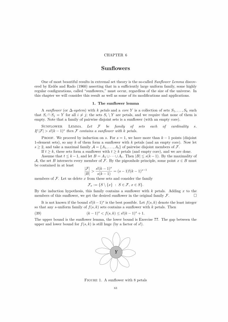
CHAPTER 6
Sunflowers
One of most beautiful results in extremal set theory is the so-called Sunflower Lemma discov-ered by Erdős and Rado (1960) asserting that in a sufficiently large uniform family, some highlyregular configurations, called “sunflowers,” must occur, regardless of the size of the universe. Inthis chapter we will consider this result as well as some of its modifications and applications.
1. The sunflower lemma
A sunflower (or ∆-system) with k petals and a core Y is a collection of sets S1, . . . , Sk suchthat Si ∩ Sj = Y for all i 6= j; the sets Si \ Y are petals, and we require that none of them isempty. Note that a family of pairwise disjoint sets is a sunflower (with an empty core).
Sunflower Lemma. Let F be family of sets each of cardinality s.If |F| > s!(k − 1)s then F contains a sunflower with k petals.
Proof. We proceed by induction on s. For s = 1, we have more than k − 1 points (disjoint1-element sets), so any k of them form a sunflower with k petals (and an empty core). Now lets ≥ 2, and take a maximal family A = A1, . . . , At of pairwise disjoint members of F .
If t ≥ k, these sets form a sunflower with t ≥ k petals (and empty core), and we are done.Assume that t ≤ k − 1, and let B = A1 ∪ · · · ∪ At. Then |B| ≤ s(k − 1). By the maximality of
A, the set B intersects every member of F . By the pigeonhole principle, some point x ∈ B mustbe contained in at least
|F||B| >
s!(k − 1)s
s(k − 1)= (s − 1)!(k − 1)s−1
members of F . Let us delete x from these sets and consider the family
Fx := S \ x : S ∈ F , x ∈ S.
By the induction hypothesis, this family contains a sunflower with k petals. Adding x to themembers of this sunflower, we get the desired sunflower in the original family F .
It is not known if the bound s!(k −1)s is the best possible. Let f(s, k) denote the least integerso that any s-uniform family of f(s, k) sets contains a sunflower with k petals. Then
(39) (k − 1)s < f(s, k) ≤ s!(k − 1)s + 1.
The upper bound is the sunflower lemma, the lower bound is Exercise ??. The gap between theupper and lower bound for f(s, k) is still huge (by a factor of s!).
Y
Figure 1. A sunflower with 8 petals
63

64 6. SUNFLOWERS
Conjecture 6.1 (Erdős and Rado). For every fixed k there is a constant C = C(k) such thatf(s, k) < Cs.
The conjecture remains open even for k = 3 (note that in this case the sunflower lemmarequires at least s!2s ≈ ss sets). Several authors have slightly improved the bounds in (??). Inparticular, J. Spencer has proved
f(s, 3) ≤ ec√
ss!.
For s fixed and k sufficiently large, Kostochka et al. (1999) have proved
f(s, k) ≤ ks(
1 + ck−2−s)
,
where c is a constant depending only on s.But the proof or disproof of the conjecture is nowhere in sight.A family F = S1, . . . , Sm is called a weak ∆-system if there is some λ such that |Si ∩Sj | = λ
whenever i 6= j. Of course, not every such system is a sunflower: in a weak ∆-system it is enoughthat all the cardinalities of mutual intersections coincide whereas in a sunflower we require thatthese intersections all have the same elements. However, the following interesting result due toM. Deza states that if a weak ∆-system has many members then it is, in fact, “strong,” i.e., formsa sunflower. We state this result without proof.
Theorem 6.2 (Deza 1973). Let F be an s-uniform weak ∆-system. If |F| ≥ s2 − s + 2 thenF is a sunflower.
The family of lines in a projective plane of order s − 1 shows that this bound is optimal (seeExercise ??).
A related problem is to estimate the maximal possible number F (n, k) of members in a familyF of subsets of an n-element set such that F does not contain a weak ∆-system with k members.It is known that
20.01(n ln n)1/3 ≤ F (n, 3) ≤ 1.99n.
The upper bound was proved by Frankl and Rödl (1987), and the lower bound by Kostochka andR"odl (1998).
2. Modifications
Due to its importance, the sunflower lemma was modified in various directions. If S1, . . . , Sk
form a sunflower with a core Y , then we have two nice properties:
(a): the core Y lies entirely in all the sets S1, . . . , Sk;(b): the sets S1 \ Y, . . . , Sk \ Y are mutually disjoint.
It is therefore natural to look at what happens if we relax any of these two conditions.
2.1. Relaxed core. We can relax property (a) and require that only the differences Si \ Ybe non-empty and mutually disjoint for some set Y .
Given distinct finite sets S1, . . . , Sk, their common part is the set
Y :=⋃
i6=j
(Si ∩ Sj) .
Note that, if |Y | < mini |Si| then all the sets S1 \Y, . . . , Sk \Y are nonempty and mutually disjoint.
Lemma 6.3 (Füredi 1980). Let F be a finite family of sets, and s = maxS∈F |S|. If |F| >(k − 1)s then the common part of some k of its members has fewer than s elements.
Proof. We prove a contraposition of this claim: If the common part of every k members of Fhas at least s = maxS∈F |S| elements, then |F| ≤ (k − 1)s. The cases k = 2 and s = 1 are trivial.Apply induction on k. Once k is fixed, apply induction on s. Let S0 be an arbitrary member ofF of size s. We have
(40) |F| = 1 +∑
X⊂S0
|S ∈ F : S ∩ S0 = X| .

3. APPLICATIONS 65
Fix now an arbitrary X ⊂ S0, and consider the family
FX := S \ S0 : S ∈ F , S ∩ S0 = X .
The maximum size of its member is s′ ≤ s−|X|. Moreover, the common part of any its k′ = k −1members S1 \ S0, . . . , Sk−1 \ S0 is the common part of k members S0, S1, . . . , Sk−1 of F minusX, and hence is at least s − |X| ≥ s′. We can therefore apply the induction hypothesis withs′ ≤ s − |X|, k′ = k − 1 and deduce
(41) |FX | ≤ (k − 2)s−|X| .
Combining (??) and (??) we obtain
|F| ≤ 1 +∑
X⊂S0
(k − 2)s−|X| ≤s∑
i=0
(s
i
)(k − 2)s−i = (k − 1)s ,
as desired.
2.2. Relaxed disjointness. What if we relax the disjointness property (b) of sunflowers,and only require that the differences S1 \ Y, . . . , Sk \ Y cannot be intersected (blocked) by a set ofsize smaller than some number t? In this case we say that sets S1, . . . , Sk form a “flower” with tpetals.
A blocking set of a family F is a set which intersects all the members of F ; the minimumnumber of elements in a blocking set is the blocking number of F and is denoted by τ(F); if ∅ ∈ Fthen we set τ(F) = 0. A restriction of a family F onto a set Y is the family
FY := S \ Y : S ∈ F , S ⊇ Y .
A flower with k petals and a core Y is a family F such that τ(FY ) ≥ k. Note that every sunflwoveris a flower with the same number of petals, but not every flower is a sunflower (give an example).
Håstad et al. (1995) observed that the proof of the sunflower lemma can be easily modified toyield a similar result for flowers.
Lemma 6.4. Let F be a family of sets each of cardinality s, and k ≥ 1 and integer. If|F| > (k − 1)s then F contains a flower with k petals.
Proof. Induction on s. The basis s = 1 is trivial since then F consists of at least k distinctsingle-element sets. Now suppose that the lemma is true for s−1 and prove it for s. Take a familyF of sets each of cardinality s, and assume that |F| > (k − 1)s. If τ(F) ≥ k then the family Fitself is a flower with at least (k − 1)s + 1 ≥ k petals (and an empty core). Otherwise, some set ofsize k − 1 intersects all the members of F , and hence, at least |F|/(k − 1) of the members mustcontain some point x. The family
Fx := S \ x : S ∈ F , x ∈ Shas
|Fx| ≥ |F|k − 1
> (k − 1)s−1
members, each of cardinality s − 1. By the induction hypothesis, the family Fx contains a flowerwith k petals and some core Y , x 6∈ Y . Adding the element x back to the sets in this flower, weobtain a flower in F with the same number of petals and the core Y ∪ x.
3. Applications
The sunflower lemma and its modifications have many applications in complexity theory. Inparticular, the combinatorial part of the celebrated lower bounds argument for monotone cir-cuits, found by Razborov (1985), is based on this lemma and on its modification due to Füredi(Lemma ??). Andreev (1987) has also used his modification (Exercise ??) to prove exponentiallower bounds for such circuits. In this section we will show how the last modification (Lemma ??)can be used to obtain some information about the number of minterms and to prove lower boundsfor small depth non-monotone circuits.

66 6. SUNFLOWERS
3.1. The number of minterms. Let x1, . . . , xn be boolean variables taking their values in0, 1. A monomial is an And of literals, and a clause is an Or of literals, where a literal is eithera variable xi or its negation xi = xi ⊕ 1. Thus, we have 2s
(ns
)monomials and that many clauses
of size s.A 1-term of a boolean function f : 0, 1n → 0, 1 is a monomial M such that M(a) ≤ f(a)
for all inputs a ∈ 0, 1n. That is, if we set all literals of M to 1, then the function f is forced totake value 1 independent on what values we assign to the remaining variables. Dually, a 0-term off is a clause C such that C(a) ≥ f(a) for all inputs a ∈ 0, 1n. A minterm of f is a 1-term M
of f which is minimal in the sense that deleting every single literal from M already violates thisproperty.
A boolean function f is a t-And-Or (or a t-CNF) if it can be written as an And of an arbitrarynumber of clauses, each of size at most t.
Lemma 6.5. Let f be a t-And-Or function on n variables. Then for every s = 1, . . . , n thefunction f has at most ts minterms of size s.
Proof. Let f = C1 ∧ · · · ∧ Cm, where each clause Ci has size at most t. We interpret theclauses as sets of their literals, and let C = C1, . . . , Cm be the corresponding family of thesesets. Let F be the family of all minterms of f that have size s (we look at minterms as sets oftheir literals). Then every set in C intersects each set in F (see Exercise ??).
Suppose that |F| > ts. Then, by Lemma ??, F has a flower with t + 1 petals. That is, thereexists a set of literals Y such that no set of at most t literals can intersect all the members of thefamily
FY = M \ Y : M ∈ F , M ⊇ Y .
The set Y is a proper part of at least one minterm of f , meaning that Y cannot intersect all theclauses in C. Take a clause C ∈ C such that C ∩ Y = ∅. Since this clause intersects all the sets inF , this means that it must intersect all the sets in FY . But this is impossible because C has sizeat most t.
3.2. Small depth formulas. An s-threshold function is a monotone boolean function T ns
which accepts a 0-1 vector if and only if it has at least s ones. That is,
T ns (x1, . . . , xn) = 1 if and only if x1 + · · · + xn ≥ s.
This function can be computed by the following formula:
T ns (x1, . . . , xn) =
∨
I : |I|=s
∧
i∈I
xi.
This formula is monotone (has no negated literals) and has depth 2 (there are only two alternationsbetween And and Or operations). But the size of this formula (the number of literals in it) iss(
ns
). Can T n
s be computed by a substantially smaller formula if we allow negated literals and/ora larger depth?
Håstad (1986) proved that, for s = ⌊n/2⌋, each such formula computing T ns must have size
exponential in n, even if we allow any constant depth, i.e., any constant number of alternations ofAnd’s and Or’s. Razborov (1987) has proved that the same holds even if we allow sum modulo 2as an additional operation. Both these proofs employ non-trivial machinery: the switching lemmaand approximations of boolean functions by low-degree polynomials.
On the other hand, Håstad et al. (1995) have shown that, at least for depth-3, one can deducethe same lower bound in an elementary way using the flower lemma (Lemma ??). In fact, theirproof holds for depth-3 circuits but, to demonstrate the idea, it is enough to show how it worksfor special depth-3 formulas.
An Or-And-Or formula is a formula of the form
(42) F = F1 ∨ F2 ∨ · · · ∨ Ft,
where each Fi is an And-Or formula, that is, each Fi is an And of an arbitrary number of clauses,each clause being an Or of literals (variables or their negations). We say that such a formula

3. APPLICATIONS 67
has bottom fan-in k if each of its clauses has at most k positive literals (the number of negatedvariables may be arbitrary). The size of a formula is the total number of literals in it.
At this point, let us note that the condition on bottom fan-in is not crucial: if the size of Fis not too large then it is possible to set some small number of variables to constant 1 so that theresulting formula will already satisfy this condition (see Exercise ??).
The idea of Håstad et al. (1995) is accumulated in the following lemma.
Lemma 6.6. Let F = F1 ∨ F2 ∨ · · · ∨ Ft be an Or-And-Or formula of bottom fan-in k. Supposethat F rejects all vectors with fewer than s ones. Then F cannot accept more than tks vectorswith precisely s ones.
Note that this lemma immediately implies that every Or-And-Or formula of bottom fan-in kcomputing the threshold function T n
s has size at least(
n
s
)k−s >
( n
ks
)s
.
Proof. Suppose that F accepts more than tks vectors with precisely s ones. Then some ofits And-Or subformulas Fi accepts more than ks of such vectors. Let A be this set of vectors withs ones accepted by Fi; hence
|A| > ks.
The formula Fi has the formFi = C1 ∧ C2 ∧ · · · ∧ Cr,
where C1, . . . , Cr are clauses with at most k positive literals in each of them. Let B be the setof all vectors with at most s − 1 ones. All these vectors must be rejected by Fi, since they arerejected by the whole formula F . Our goal is to show that the set B contains a vector v on whicheach of the clauses C1, . . . , Cr outputs the same value as on some vector from A; this will meanthat the formula Fi makes an error on this input – it is forced to accept v.
Say that a vector v is a k-limit for A if, for every subset S of k coordinates, there exists avector u ∈ A such that v ≤ u (vector comparision) and v coincides with u in all the coordinatesfrom S; that is, vi ≤ ui for all i and vi = ui for all i ∈ S.
Claim 6.7. There exists a vector v ∈ B which is a k-limit for A.
Proof of Claim ??. For a vector u ∈ 0, 1n, let Eu be the corresponding subset of 1, . . . , n,whose incidence vector is u, that is, Eu = i : ui = 1. Consider the family F = Eu : u ∈ A.This family is s-uniform and has more than ks members. By Lemma ??, F has a flower withk + 1 petals. That is, there exists a set Y such that no set of size at most k can intersect all themembers of the family FY = E \ Y : E ∈ F , E ⊇ Y . Let v be the incidence vector of Y . Weclaim that v is a k-limit for A.
To show this, take an arbitrary subset S of 1, . . . , n of size at most k. Then
(43) S ∩ (Eu \ Y ) = ∅for at least one set Eu ∈ F such that Y ⊆ Eu. The last condition implies that v ≤ u, and hence, vcoincides with u on all coordinates from S \ Eu and from S ∩ Y . But, by (??), there are no othercoordinates in S, and hence, v coincides with u on all coordinates from S, as desired.
Fix a vector v guaranteed by the claim. To get the desired contradiction we will show that theformula Fi will be forced to (wrongly) accept this vector. Suppose the opposite that v is rejectedby Fi. Then C(v) = 0 for some clause C of Fi. This clause has a form
C =
( ∨
i∈S
xi
)∨( ∨
j∈T
xj
)
for some two disjoint sets of S, T such that |S| ≤ k. By Claim ??, there is a vector u in A suchthat v ≤ u and v coincides with u on all the coordinates from S. The vector u must be acceptedby the formula Fi, and hence, by the clause C. This can happen only if this vector has a 1 insome coordinate i ∈ S or has a 0 in some coordinate j ∈ T (or both). In the first case C(v) = 1

68 6. SUNFLOWERS
because v coincides with u on S, and in the second case C(v) = 1 because, due to the conditionv ≤ u, vector v has 0s in all coordinates where vector u has them. Thus, in both cases, C(v) = 1,a contradiction.
Exercises
Ex 6.1. A projective plane of order s−1 is a family of n = s2 −s+1 s-element subsets (calledlines) of an n-element set of points such that each two lines intersect in precisely one point andeach point belongs to precisely s lines (cf. Sect. ??). Show that the equality in Deza’s theorem(Theorem ??) is attained when a projective plane of order s − 1 exists.
Ex 6.2. Take s pairwise disjoint (k − 1)-element sets V1, . . . , Vs and consider the family
F = S : |S| = s and |S ∩ Vi| = 1 for all i = 1, . . . , s.
This family has (k − 1)s sets. Show that it has no sunflower with k petals.
Ex 6.3. Show that the bounds in Lemmas ??, and ?? are optimal. Hint: Consider the familydefined in the previous exercise.
Ex 6.4. A matching of size k in a graph is a set of its k pairwise disjoint edges (two edgesare disjoint if they have no vertex in common). A star of size k is a set of k edges incident to onevertex. Argue as in the proof of the sunflower lemma to show that any set of more than 2(k − 1)2
edges either contains a matching of size k or a star of size k.
Ex 6.5. (Andreev 1987). Let F be a family of sets each of cardinality at most s, and supposethat |F| > (k−1)s. Use the argument of Lemma ?? to prove that then there exist k sets S1, . . . , Sk
in F such that all the sets Si \ (S1 ∩ S2), i = 1, . . . , k are pairwise disjoint.
Ex 6.6. Let n−k+1 < s ≤ n and consider the family F of all s-element subsets of a n-elementset. Prove that F has no sunflower with k petals. Hint: Suppose the opposite and count the numberof elements used in such a sunflower.
Ex 6.7. Given a graph G = (V, E) and a number 2 ≤ s ≤ |V |, let Gs denote the graph whosevertices are all s-element subsets of V , and two such subsets A and B are connected by an edgeif and only if there is an edge (u, v) ∈ E such that u ∈ A \ B and v ∈ B \ A. Suppose that thegraph G is “sparse” in the following sense: every subset of at most ks vertices spans fewer that(
k2
)edges. Use Lemma ?? to show that then Gs has no clique of size larger than (k −1)s. Hint: Let
F be a clique in Gs, and suppose that F forms a flower with k petals. Then each member A ∈ F containsan element vA which is not contained in any other member of F . Use the fact that F was a clique in Gs
to argue that vA : A ∈ F is a clique in G.
Ex 6.8. For a graph G, let G be a graph whose vertices are all maximum cliques of G, andwhere two such cliques A and B are connected by an edge if and only if there is an edge (u, v) ∈ Esuch that u ∈ A \ B and v ∈ B \ A. Recall that a clique is a maximum clique if each of remainingvertices is not connected to at least one of its edges (i.e. we cannot add any new vertices). Letα(G) denote the independence number of G, that is, the maximum number of vertices no two ofwhich are adjacent in G. Show that α(G) ≤ α(G). Hint: Let F be an independent set in G. Showthat then for any three distinct members A, B and K of F , the intersections A ∩ K and B ∩ K must becomparable by set-inclusion. Argue that then each member K ∈ F must contain an element vK whichbelongs to none of the remaining members. Why is then the set vK : K ∈ F an independent set in G?
Ex 6.9. Show that every 0-term C and every 1-term K of a boolean function f must share atleast one literal in common. Hint: Take a restriction (a partial assignment to variables) which evaluatesall the literals of K to 1. If C has no literal of K, then this restriction can be extended to an input a suchthat f(a) = 0.
Ex 6.10. Let F be a set of clauses on n variables. Say that a clause is long if it has at leastk + 1 positive literals. Let ℓ be the number of long clauses in F , and suppose that
ℓ <
(n + 1
m + 1
)k
.

EXERCISES 69
Prove that then it is possible to assign some n − m variables to constant 1 so that the resultingset F ′ will have no long clauses. Hint: Construct the desired set assignment via the following “greedy”procedure: Take the variable xi1 which occurs in the largest number of long clauses and set it to 1; thentake the variable xi2 which occurs in the largest number of remaining long clauses and set it to 1, and soon, until all long clauses dissapear (get value 1). In computations use the estimate
∑n
i=1i−1 ∼ ln n.
Ex 6.11. Consider the following function on n = sr variables:
f =
s∧
i=1
r∨
j=1
xij .
Let F be an Or-And-Or formula of bottom fan-in k (k ≤ r) computing this function. Show thatthen F has size at least (r/k)s. Hint: Observe that f rejects all vectors with fewer than s ones andaccepts rs vectors with precisely s ones; apply Lemma ??.
Ex 6.12. (Håstad et al. 1995). Consider the function on n = m2 variables defined by theformula
f =
m∧
i=1
m∨
j=1
xij ∧ yij .
This formula is a depth-3 And-Or-And formula of size only 2n. Prove that any depth-3 Or-And-Orformula for this function has size at least 2Ω(
√n). Hint: Assume that f has such a formula F of size at
most 2m/3. Reduce the bottom fan-in of F to k = ⌈m/2⌉ by setting one half of the variables to constantsat random as follows: for each pair of variables xij , yij , pick one of them at random (with probability 1/2)and set it to 1. If some clause has more than k positive literals, then none of these literals is set to 1 withprobability at most 2−k−1. The probability, that some of the clauses with more than k positive literals isnot evaluated to 1, does not exceed 2m/3 · 2−(k+1) ≤ 2−m/6 < 1, and in particular such a setting exists.The resulting function has the same form as that considered in the previous exercise.

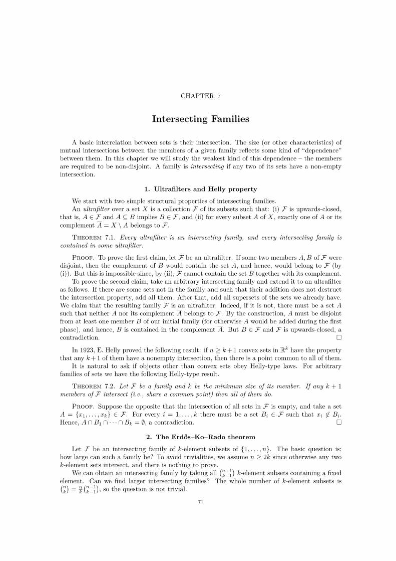
CHAPTER 7
Intersecting Families
A basic interrelation between sets is their intersection. The size (or other characteristics) ofmutual intersections between the members of a given family reflects some kind of “dependence”between them. In this chapter we will study the weakest kind of this dependence – the membersare required to be non-disjoint. A family is intersecting if any two of its sets have a non-emptyintersection.
1. Ultrafilters and Helly property
We start with two simple structural properties of intersecting families.An ultrafilter over a set X is a collection F of its subsets such that: (i) F is upwards-closed,
that is, A ∈ F and A ⊆ B implies B ∈ F , and (ii) for every subset A of X, exactly one of A or itscomplement A = X \ A belongs to F .
Theorem 7.1. Every ultrafilter is an intersecting family, and every intersecting family iscontained in some ultrafilter.
Proof. To prove the first claim, let F be an ultrafilter. If some two members A, B of F weredisjoint, then the complement of B would contain the set A, and hence, would belong to F (by(i)). But this is impossible since, by (ii), F cannot contain the set B together with its complement.
To prove the second claim, take an arbitrary intersecting family and extend it to an ultrafilteras follows. If there are some sets not in the family and such that their addition does not destructthe intersection property, add all them. After that, add all supersets of the sets we already have.We claim that the resulting family F is an ultrafilter. Indeed, if it is not, there must be a set Asuch that neither A nor its complement A belongs to F . By the construction, A must be disjointfrom at least one member B of our initial family (for otherwise A would be added during the firstphase), and hence, B is contained in the complement A. But B ∈ F and F is upwards-closed, acontradiction.
In 1923, E. Helly proved the following result: if n ≥ k + 1 convex sets in Rk have the propertythat any k + 1 of them have a nonempty intersection, then there is a point common to all of them.
It is natural to ask if objects other than convex sets obey Helly-type laws. For arbitraryfamilies of sets we have the following Helly-type result.
Theorem 7.2. Let F be a family and k be the minimum size of its member. If any k + 1members of F intersect (i.e., share a common point) then all of them do.
Proof. Suppose the opposite that the intersection of all sets in F is empty, and take a setA = x1, . . . , xk ∈ F . For every i = 1, . . . , k there must be a set Bi ∈ F such that xi 6∈ Bi.Hence, A ∩ B1 ∩ · · · ∩ Bk = ∅, a contradiction.
2. The Erdős–Ko–Rado theorem
Let F be an intersecting family of k-element subsets of 1, . . . , n. The basic question is:how large can such a family be? To avoid trivialities, we assume n ≥ 2k since otherwise any twok-element sets intersect, and there is nothing to prove.
We can obtain an intersecting family by taking all(
n−1k−1
)k-element subsets containing a fixed
element. Can we find larger intersecting families? The whole number of k-element subsets is(nk
)= n
k
(n−1k−1
), so the question is not trivial.
71
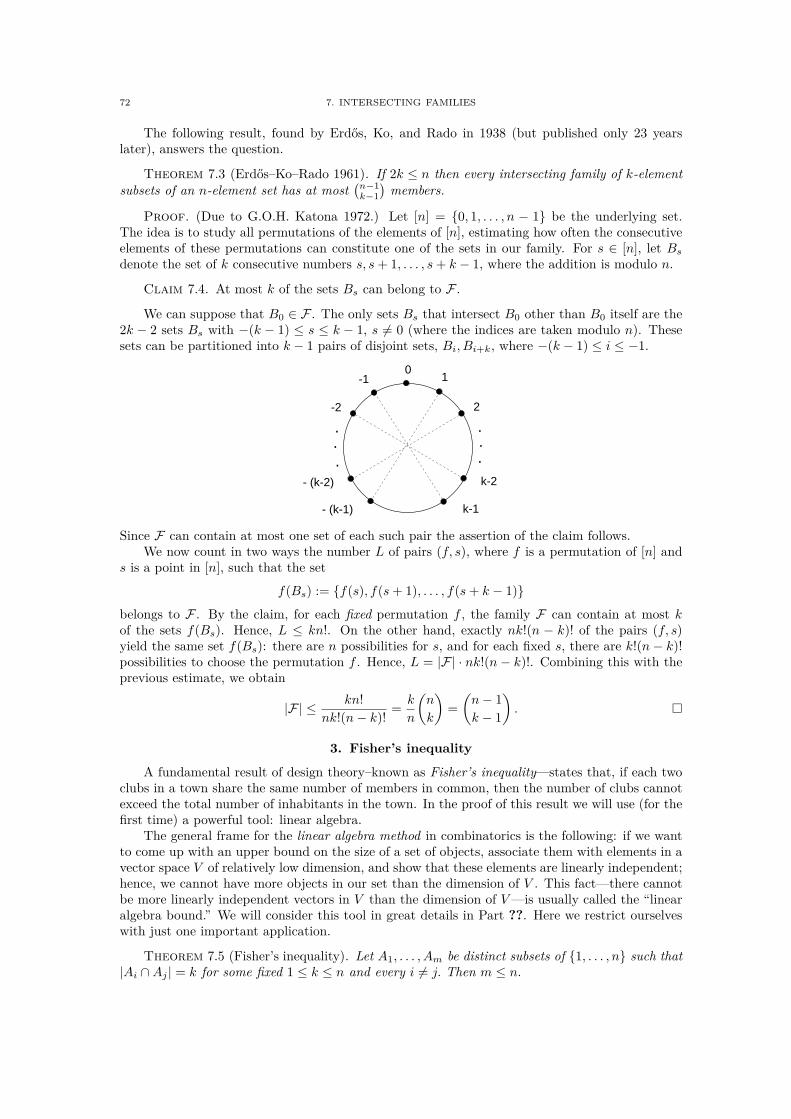
72 7. INTERSECTING FAMILIES
The following result, found by Erdős, Ko, and Rado in 1938 (but published only 23 yearslater), answers the question.
Theorem 7.3 (Erdős–Ko–Rado 1961). If 2k ≤ n then every intersecting family of k-elementsubsets of an n-element set has at most
(n−1k−1
)members.
Proof. (Due to G.O.H. Katona 1972.) Let [n] = 0, 1, . . . , n − 1 be the underlying set.The idea is to study all permutations of the elements of [n], estimating how often the consecutiveelements of these permutations can constitute one of the sets in our family. For s ∈ [n], let Bs
denote the set of k consecutive numbers s, s + 1, . . . , s + k − 1, where the addition is modulo n.
Claim 7.4. At most k of the sets Bs can belong to F .
We can suppose that B0 ∈ F . The only sets Bs that intersect B0 other than B0 itself are the2k − 2 sets Bs with −(k − 1) ≤ s ≤ k − 1, s 6= 0 (where the indices are taken modulo n). Thesesets can be partitioned into k − 1 pairs of disjoint sets, Bi, Bi+k, where −(k − 1) ≤ i ≤ −1.
1-1
- (k-2)
- (k-1)
k-2
k-1
2-2
...
.
.
.
0
Since F can contain at most one set of each such pair the assertion of the claim follows.We now count in two ways the number L of pairs (f, s), where f is a permutation of [n] and
s is a point in [n], such that the set
f(Bs) := f(s), f(s + 1), . . . , f(s + k − 1)belongs to F . By the claim, for each fixed permutation f , the family F can contain at most kof the sets f(Bs). Hence, L ≤ kn!. On the other hand, exactly nk!(n − k)! of the pairs (f, s)yield the same set f(Bs): there are n possibilities for s, and for each fixed s, there are k!(n − k)!possibilities to choose the permutation f . Hence, L = |F| · nk!(n − k)!. Combining this with theprevious estimate, we obtain
|F| ≤ kn!
nk!(n − k)!=
k
n
(n
k
)=
(n − 1
k − 1
).
3. Fisher’s inequality
A fundamental result of design theory–known as Fisher’s inequality—states that, if each twoclubs in a town share the same number of members in common, then the number of clubs cannotexceed the total number of inhabitants in the town. In the proof of this result we will use (for thefirst time) a powerful tool: linear algebra.
The general frame for the linear algebra method in combinatorics is the following: if we wantto come up with an upper bound on the size of a set of objects, associate them with elements in avector space V of relatively low dimension, and show that these elements are linearly independent;hence, we cannot have more objects in our set than the dimension of V . This fact—there cannotbe more linearly independent vectors in V than the dimension of V —is usually called the “linearalgebra bound.” We will consider this tool in great details in Part ??. Here we restrict ourselveswith just one important application.
Theorem 7.5 (Fisher’s inequality). Let A1, . . . , Am be distinct subsets of 1, . . . , n such that|Ai ∩ Aj | = k for some fixed 1 ≤ k ≤ n and every i 6= j. Then m ≤ n.

4. MAXIMAL INTERSECTING FAMILIES 73
Proof. For two vectors x, y ∈ Rn, let 〈x, y〉 = x1y1 + · · · + xnyn denote their scalar product.Let v1, . . . , vm ∈ 0, 1n be incidence vectors of A1, . . . , Am. By the linear algebra bound it isenough to show that these vectors are linearly independent over the reals. Assume the contrary,i.e., that the linear relation
∑mi=1 λivi = 0 exists, with not all coefficients being zero. Obviously,
〈vi, vj〉 = |Ai| if j = i, and 〈vi, vj〉 = k if j 6= i. Consequently,
0 =
( m∑
i=1
λivi
)( m∑
j=1
λjvj
)=
m∑
i=1
λ2i 〈vi, vi〉 +
∑
1≤i6=j≤m
λiλj〈vi, vj〉
=
m∑
i=1
λ2i |Ai| +
∑
1≤i6=j≤m
λiλjk =
m∑
i=1
λ2i (|Ai| − k) + k ·
( m∑
i=1
λi
)2
.
Clearly, |Ai| ≥ k for all i and |Ai| = k for at most one i, since otherwise the intersection conditionwould not be satisfied. But then the right-hand is greater than 0 (because the last sum can vanishonly if at least two of the coefficients λi are nonzero), a contradiction.
This theorem was first proved by the statistician R. A. Fisher in 1940 for the case whenk = 1 and all sets Ai have the same size (such configurations are known as balanced incompleteblock designs). In 1948, de Bruijn and Erdős relaxed the uniformity condition for the sets Ai (seeTheorem ??). This was generalized by R. C. Bose in 1949, and later by several other authors.But it was the two-page paper of Bose where the linear argument was first applied to solve acombinatorial problem. The general version, stated above, was first proved by Majumdar (1953);the proof we presented is a variation of a simplified argument found by Babai and Frankl (1992).
4. Maximal intersecting families
Let F be a k-uniform family of sets of some n-element set. Say that F is maximal intersectingif
(i) F is intersecting;(ii) the addition of any new k-element set to F destroys this property, that is, for every k-element
subset E 6∈ F , the family F ∪ E is no longer intersecting.
The case when n ≤ 2k − 1 is not interesting, because then the only maximal intersecting familyis the family of all k-element subsets. But what if n ≥ 2k? Intuitively, any maximal intersectingfamily must be large enough, because every k-element set not in the family must be avoided byat least one of its members. It is therefore interesting to investigate the minimal possible numberf(k) of members which such a family can have.
To give an upper bound on f(k), consider the family F of lines in a projective plane oforder k − 1 (see Sect. ??). For our current purposes it is enough to know that F is a family of|F| = n = k2 − k + 1 k-element subsets (called lines) of an n-element set of points such that eachtwo lines intersect in precisely one point and each point belongs to precisely k lines. It is easy toshow that this family is maximal intersecting (see Exercise ??). Hence, f(k) ≤ k2 − k + 1 for allthose values of k for which a projective plane of order k − 1 exists.
In the case of projective planes, we have a k-uniform family with about k2 sets. But thenumber of points in this case is also the same. What if we take a lot fewer than k2 points?Can we then still find a k-uniform and maximal intersecting family of size at most k2? Usingdouble-counting we can answer this question negatively.
Theorem 7.6 (Füredi 1980). Let F be a maximal intersecting family of k-element sets of ann-element set. If n ≤ k2/2 log k, then F must have more than k2 members.
Proof. To simplify computations, we only prove the theorem under a slightly stronger as-sumption that n ≤ k2/(1+2 log k). The idea is to count in two ways the number N of pairs (F, E)where F ∈ F and E is a k-element subset disjoint from F (and hence, E 6∈ F). Since every suchset E must be avoided by at least one member of F , N ≥
(nk
)− |F| . On the other hand, each
member of F can avoid at most(
n−kk
)of the sets E; hence N ≤ |F|·
(n−k
k
). These two inequalities,

74 7. INTERSECTING FAMILIES
together with the estimate (??), imply
|F| ≥(
nk
)
1 +(
n−kk
) ≥ 1
2·(
n
n − k
)k
> ek2/n−1 ≥ e2 log k ≥ k2 .
Now suppose that F1, . . . , Fm are intersecting (not necessarily uniform) families of an n-element set 1, . . . , n. How many sets can we have in their union?
Taking each Fi to be the family of all 2n−1 subsets containing the element i, we see that theunion will have 2n − 2n−m sets.
A beautiful result, due to Kleitman, says that this bound is best possible.
Theorem 7.7 (Kleitman 1966). The union of m intersecting families contains at most 2n −2n−m sets.
Proof. We apply induction on m. The case m = 1 being trivial, we turn to the inductionstep. We say that a family A is monotone increasing (monotone decreasing) if A ∈ A and B ⊇ A(respectively, B ⊆ A) implies B ∈ A. A famous result, also due to Kleitman (we will prove it inSect. ??; see Theorem ?? and Exercise ??) says that, if A is a monotone decreasing and B is amonotone increasing family of subsets of an n-element set, then
(44) |A ∩ B| ≤ 2−n|A| · |B| .
Now let F =⋃m
i=1 Fi, with each Fi being an intersecting family. Since our aim is to bound|F| from the above, we may assume that each Fi is maximal intersecting family; in particular,|Fm| = 2n−1. Let A be the complement of Fm, i.e., the family of all |A| = 2n−1 subsets not in Fm,
and B =⋃m−1
i=1 Fi. Since F1, . . . , Fm are maximal intersecting families, A is monotone decreasingand B is monotone increasing. By the induction hypothesis, |B| ≤ 2n − 2n−m+1, and, by (??),
|A ∩ B| ≤ 2−n2n−1(2n − 2n−m+1) = 2n−1 − 2n−m .
Therefore,|B ∩ Fm| = |B| − |A ∩ B| ≥ |B| − 2n−1 + 2n−m
and
|F| =
∣∣∣∣m⋃
i=1
Fi
∣∣∣∣ = |B| + |Fm| − |B ∩ Fm| ≤ 2n − 2n−m .
5. Cross-intersecting families
A pair of families A, B is cross-intersecting if every set in A intersects every set in B. Therank of A is the maximum cardinality of a set in A. The degree dA(x) of a point x in A is thenumber of sets in A containing x.
If A has rank a, then, by the pigeonhole principle, each set in A contains a point x whichis “popular” for the members of B in that dB(x) ≥ |B|/a. Similarly, if B has rank b, then eachmember of B contains a point y for which dA(y) ≥ |A|/b. However, this alone does not imply thatwe can find a point which is popular in both families A and B. It turns out that if we relax the“degree of popularity” by one-half, then such a point exists.
Theorem 7.8 (Razborov–Vereshchagin 1999). Let A be a family of rank a and B be a familyof rank b. Suppose that the pair A, B is cross-intersecting. Then there exists a point x such that
dA(x) ≥ |A|2b
and dB(x) ≥ |B|2a
.
Proof. Assume the contrary and let A, B be independent random sets that are uniformlydistributed in A, B respectively. That is, for each A ∈ A and B ∈ B, Pr [A = A] = 1/|A|and Pr [B = B] = 1/|B|. Since the pair A, B is cross-intersecting, the probability of the event“∃x(x ∈ A ∩ B)” is equal to 1. Since the probability of a disjunction of events is at most the sumof the probabilities of the events, we have
∑
x
Pr [x ∈ A ∩ B] ≥ 1.

EXERCISES 75
Let X0 consist of those points x for which
dA(x)
|A| = Pr [x ∈ A] <1
2b,
and X1 consist of the remaining points. Note that by our assumption, for any x ∈ X1,
Pr [x ∈ B] =dB(x)
|B| <1
2a
holds. By double counting (see Proposition ??),∑
x dA(x) =∑
A∈A |A|. Hence,∑
x∈X1
Pr [x ∈ A ∩ B] =∑
x∈X1
Pr [x ∈ A] · Pr [x ∈ B]
<1
2a·∑
x∈X1
Pr [x ∈ A] ≤ 1
2a·∑
x
Pr [x ∈ A]
=1
2a·∑
x
dA(x)
|A| =1
2a|A| ·∑
x
dA(x) =1
2a|A| ·∑
A∈A|A| ≤ a|A|
2a|A| =1
2.
In a similar way we obtain∑
x∈X0
Pr [x ∈ A ∩ B] <1
2,
a contradiction.
We mention (without proof) the following related result.
Theorem 7.9 (Füredi 1995). Let a + b ≤ n, A be a family of a-element sets and B a family
of b-element sets on the common underlying set [n] such that |A| ≥(
n−1a−1
)−(
n−b−1a−1
)+ 1 and
|B| ≥(
n−1b−1
)−(
n−a−1b−1
)+1. If the pair A, B is cross-intersecting, then some element x ∈ [n] belongs
to all members of A and B.
Exercises
Ex 7.1. Let F be a family of subsets of an n-element set. Prove that if F is intersecting then|F| ≤ 2n−1. Is this the best bound? If so, then exhibit an intersecting family with |F| = 2n−1.Hint: A set and its complement cannot both be the members of F .
Ex 7.2. Let F be an intersecting family of subsets of an n-element set X. Show that there isan intersecting family F ′ ⊇ F such that |F| = 2n−1. Hint: Show that for any set A such that neitherA nor A belongs to F , exactly one of A and A can be added to F .
Ex 7.3. Let n ≤ 2k and let A1, . . . , Am be a family of k-element subsets of [n] such thatAi ∪ Aj 6= [n] for all i, j. Show that m ≤
(1 − k
n
) (nk
). Hint: Apply the Erdős–Ko–Rado theorem to
the complements Ai = [n] − Ai.
Ex 7.4. The upper bound(
n−1k−1
)given by Erdős–Ko–Rado theorem is achieved by the families
of sets containing a fixed element. Show that for n = 2k there are other families achieving thisbound. Hint: Include one set out of every pair of sets formed by a k-element set and its complement.
Ex 7.5. One can generalize the intersection property and require that |A ∩ B| ≥ t for allA 6= B ∈ F . Such families are called t-intersecting. The first example of a t-intersecting familywhich comes to mind, is the family of all subsets of [n] containing some fixed set of t elements.This family has 2n−t sets. Are there larger t-intersecting families? Hint: Let n + t be even and takeF =
A ⊆ [n] : |A| = n+t
2
.
Ex 7.6. Let =. B1, . . . , Bb be a (v, k, λ) design, i.e., a family of k-element subsets of a v-element set of points X = x1, . . . , xv such that every two points belong to exactly λ sets. UseFisher’s inequality to show that b ≥ v. Hint: Take Ai := j : xi ∈ Bj.

76 7. INTERSECTING FAMILIES
Ex 7.7. Consider the k-uniform family of all n = k2 − k + 1 lines in the set of points of aprojective plane of order k − 1. Clearly, this family is intersecting. Show that it is also maximalintersecting, i.e., that every k-element set E, which intersects all the lines, must be a line. Hint:Assume that E is not a line, draw a line L through some two points x 6= y of E, and take a pointz ∈ L \ x, y. This point belongs to k lines, and each of them intersect E.
Ex 7.8. (Razborov–Vereshchagin 1999). Show that the bound in Theorem ?? is tight up to amultiplicative factor of 2. Hint: Consider the following pair of families
A = A1, . . . , Ab, where Ai = (i, 1), (i, 2), . . . , (i, a),
B = B1, . . . , Ba, where Bj = (1, j), (2, j), . . . , (b, j).
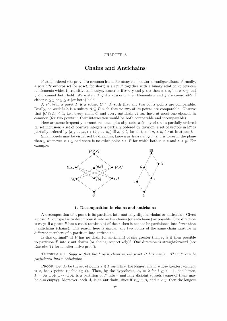
CHAPTER 8
Chains and Antichains
Partial ordered sets provide a common frame for many combinatorial configurations. Formally,a partially ordered set (or poset, for short) is a set P together with a binary relation < betweenits elements which is transitive and antysymmetric: if x < y and y < z then x < z, but x < y andy < x cannot both hold. We write x ≤ y if x < y or x = y. Elements x and y are comparable ifeither x ≤ y or y ≤ x (or both) hold.
A chain in a poset P is a subset C ⊆ P such that any two of its points are comparable.Dually, an antichain is a subset A ⊆ P such that no two of its points are comparable. Observethat |C ∩ A| ≤ 1, i.e., every chain C and every antichain A can have at most one element incommon (for two points in their intersection would be both comparable and incomparable).
Here are some frequently encountered examples of posets: a family of sets is partially orderedby set inclusion; a set of positive integers is partially ordered by division; a set of vectors in Rn ispartially ordered by (a1, . . . , an) < (b1, . . . , bn) iff ai ≤ bi for all i, and ai < bi for at least one i.
Small posets may be visualized by drawings, known as Hasse diagrams: x is lower in the planethan y whenever x < y and there is no other point z ∈ P for which both x < z and z < y. Forexample:
a,c a,b
ba c
O
b,c
a,b,c
1
23
69
18
1. Decomposition in chains and antichains
A decomposition of a poset is its partition into mutually disjoint chains or antichains. Givena poset P , our goal is to decompose it into as few chains (or antichains) as possible. One directionis easy: if a poset P has a chain (antichain) of size r then it cannot be partitioned into fewer thanr antichains (chains). The reason here is simple: any two points of the same chain must lie indifferent members of a partition into antichains.
Is this optimal? If P has no chain (or antichain) of size greater than r, is it then possibleto partition P into r antichains (or chains, respectively)? One direction is straightforward (seeExercise ?? for an alternative proof):
Theorem 8.1. Suppose that the largest chain in the poset P has size r. Then P can bepartitioned into r antichains.
Proof. Let Ai be the set of points x ∈ P such that the longest chain, whose greatest elementis x, has i points (including x). Then, by the hypothesis, Ai = ∅ for i ≥ r + 1, and hence,P = A1 ∪ A2 ∪ · · · ∪ Ar is a partition of P into r mutually disjoint subsets (some of them maybe also empty). Moreover, each Ai is an antichain, since if x, y ∈ Ai and x < y, then the longest
77

78 8. CHAINS AND ANTICHAINS
chain x1 < . . . < xi = x ending in x could be prolonged to a longer chain x1 < . . . < xi < y,meaning that y 6∈ Ai.
The dual result looks similar, but its proof is more involved. This result, uniformly known asDilworth’s Decomposition Theorem (Dilworth 1950) has played an important role in motivatingresearch into posets. There are several elegant proofs; the one we present is due to F. Galvin.
Theorem 8.2 (Dilworth’s theorem). Suppose that the largest antichain in the poset P hassize r. Then P can be partitioned into r chains.
Proof (due to Galvin 1994). We use induction on the cardinality of P . Let a be a maximal elementof P , and let r be the size of a largest antichain in P ′ = P \a. Then P ′ is the union of r disjointchains C1, . . . , Cr. We have to show that P either contains an (r + 1)-element antichain or else isthe union of r disjoint chains. Now, every r-element antichain in P ′ consists of one element fromeach Ci. Let ai be the maximal element in Ci which belongs to some r-element antichain in P ′.It is easy to see that A = a1, . . . , ar is an antichain in P ′. If A ∪ a is an antichain in P , weare done: we have found an antichain of size r + 1). Otherwise, we have a > ai for some i. ThenK = a ∪ x ∈ Ci : x ≤ ai is a chain in P , and there are no r-element antichains in P \ K (sinceai was the maximal element of Ci participating in such an antichain), whence P \ K is the unionof r − 1 chains.
To recognize the power of this theorem, let us show that it contains Hall’s Marriage Theorem ??as a special case!
Suppose that S1, . . . , Sm are sets satisfying Hall’s condition, i.e., |S(I)| ≥ |I| for all I ⊆1, . . . , m, where S(I) :=
⋃i∈I Si. We construct a poset P as follows. The points of P are the
elements of X := S1 ∪ · · · ∪ Sm and symbols y1, . . . , ym, with x < yi if x ∈ Si, and no othercomparabilities. It is clear that X is an antichain in P . We claim that there is no larger antichain.To show this, let A be an antichain, and set I := i : yi ∈ A. Then A contains no point of S(I),for if x ∈ Si then x is comparable with yi, and hence, A cannot contain both of these points.Hence, Hall’s condition implies that |A| ≤ |I| + |X| − |S(I)| ≤ |X|, as claimed.
Now, Dilworth’s theorem implies that P can be partitioned into |X| chains. Since the antichainX is maximal, each of the chains in the partition must contain a point of X. Let the chain throughyi be xi, yi. Then (x1, . . . , xm) is a desired system of distinct representatives: for xi ∈ Si (sincexi < yi) and xi 6= xj (since the chains are disjoint).
In general, Dilworth’s theorem says nothing more about the chains, forming the partition,except that they are mutually disjoint. However, if we consider special posets then we can extractmore information about the partition. To illustrate this, let us consider now the poset 2X whosepoints are all subsets of an n-element set X partially ordered by set inclusion. De Bruijn, Teng-bergen, and Kruyswijk (1952) have shown that 2X can be partitioned into disjoint chains that arealso “symmetric.”
Let C = A1, . . . , Ak be a chain in 2X , i.e., A1 ⊂ A2 ⊂ . . . ⊂ Ak. This chain is symmetric if|A1| + |Ak| = n and |Ai+1| = |Ai| + 1 for all i = 1, . . . , k − 1. “Symmetric” here means symmetricpositioned about the middle level n
2 . Symmetric chains with k = n are maximal. Maximal chainsare in one-to-one correspondence with the permutations of the underlying set: every permutation(x1, . . . , xn) gives the maximal chain
x1 ⊂ x1, x2 ⊂ . . . ⊂ x1, . . . , xn.
Theorem 8.3. The family of all subsets of an n-element set can be partitioned into(
n⌊n/2⌋
)
mutually disjoint symmetric chains.
Proof. Take an n-element set X, and assume for a moment that we already have somepartition of 2X into symmetric chains. Every such chain contains exactly one set from the middlelevel; hence there are
(n
⌊n/2⌋)
chains in that partition.
Let us now prove that such a partition is possible at all. We argue by the induction on n = |X|.Clearly the result holds for the one point set X. So, suppose that it is true for all sets with fewerpoints then n. Pick a point x ∈ X, and let Y := X \ x. By induction, we can partition 2Y into

2. APPLICATION: THE MEMORY ALLOCATION PROBLEM 79
symmetric chains C1, . . . , Cr. Each of these chains over Y
Ci := A1 ⊂ A2 ⊂ . . . ⊂ Ak
produce the following two chains over the whole set X:
C′i := A1 ⊂ A2 ⊂ . . . ⊂ Ak−1 ⊂ Ak ⊂ Ak ∪ x
C′′i := A1 ∪ x ⊂ A2 ∪ x ⊂ . . . ⊂ Ak−1 ∪ x.
These chains are symmetric since
|A1| + |Ak ∪ x| = (|A1| + |Ak|) + 1 = (n − 1) + 1 = n
and|A1 ∪ x| + |Ak−1 ∪ x| = (|A1| + |Ak−1|) + 2 = (n − 2) + 2 = n.
Is this a partition? It is indeed. If A ⊆ Y then only C′i contains A where Ci is the chain in 2Y
containing A. If A = B ∪ x where B ⊆ Y then B ∈ Ci for some i. If B is the maximal elementof Ci then C′
i is the only chain containing A, otherwise A is contained only in C′′i .
2. Application: the memory allocation problem
The following problem arises in information storage and retrieval. Suppose we have some list(a sequence) L = (a1, a2, . . . , am) of not necessarily distinct elements of some set X. We say thatthis list contains a subset A if it contains A as a subsequence of consecutive terms, that is, if
A = ai, ai+1, . . . , ai+|A|−1for some i. A sequence is universal for X if it contains all the subsets of X. For example, ifX = 1, 2, 3, 4, 5 then the list
L = (1 2 3 4 5 1 2 4 1 3 5 2 4)
of length m = 13 is universal for X.What is the length of a shortest universal sequence for an n-element set? Since any two sets
of equal cardinality must start from different places of this string, the trivial lower bound for the
length of universal sequence is(
n⌊n/2⌋
), which is about
√2
πn 2n, according to Stirling’s formula (??).
A trivial upper bound for the length of the shortest universal sequence is obtained by consideringthe sequence obtained simply by writing down each subset one after the other. Since there are 2n
subsets of average size n/2, the length of the resulting universal sequence is at most n2n−1. UsingDilworth’s theorem, we can obtain a universal sequence, which is n times (!) shorter than thistrivial one.
Theorem 8.4 (Lipski 1978). There is a universal sequence for 1, . . . , n of length at most2π 2n.
Proof. We consider the case when n is even, say n = 2k (the case of odd n is similar). LetS = 1, . . . , k be the set of the first k elements and T = k + 1, . . . , 2k the set of the last kelements. By Theorem ??, both S and T have symmetric chain decompositions of their posets ofsubsets into m =
(k
k/2
)symmetric chains: 2S = C1∪· · ·∪Cm and 2T = D1∪· · ·∪Dm. Corresponding
to the chain
Ci = x1, . . . , xj ⊂ x1, . . . , xj , xj+1 ⊂ . . . ⊂ x1, . . . , xh (j + h = k)
we associate the sequence (not the set!) Ci = (x1, x2, . . . xh). Then every subset of S occursas an initial part of one of the sequences C1, . . . , Cm. Similarly let D1, . . . , Dm be sequencescorresponding to the chains D1, . . . , Dm. If we let Di denote the sequence obtained by writing Di
in reverse order, then every subset of T occurs as a final part of one of the Di. Next, consider thesequence
L = D1C1D1C2 . . . D1Cm . . . DmC1DmC2 . . . DmCm.
We claim that L is a universal sequence for the set 1, . . . , n. Indeed, each of its subsets A canbe written as A = E ∪ F where E ⊆ S and F ⊆ T . Now F occurs as the final part of some Df
and E occurs as the initial part of some Ce; hence, the whole set A occurs in the sequence L asthe part of Df Ce. Thus, the sequence L contains every subset of 1, . . . , n. The length of the
80 8. CHAINS AND ANTICHAINS
sequence L is at most km2 = k(
kk/2
)2. Since, by Stirling’s formula,
(k
k/2
)∼ 2k
√2
kπ , the length of
the sequence is km2 ∼ k 2kπ · 22k = 2
π 2n.
3. Sperner’s theorem
A set system F is an antichain (or Sperner system) if no set in it contains another: if A, B ∈ Fand A 6= B then A 6⊆ B. It is an antichain in the sense that this property is the other extremefrom that of the chain in which every pair of sets is comparable.
Simplest examples of antichains over 1, . . . , n are the families of all sets of fixed cardinalityk, k = 0, 1, . . . , n. Each of these antichains has
(nk
)members. Recognizing that the maximum of(
nk
)is achieved for k = ⌊n/2⌋, we conclude that there are antichains of size
(n
⌊n/2⌋). Are these
antichains the largest ones?The positive answer to this question was found by Emanuel Sperner in 1928, and this result
is known as Sperner’s Theorem.
Theorem 8.5 (Sperner 1928). Let F be a family of subsets of an n element set. If F is anantichain then |F| ≤
(n
⌊n/2⌋).
A considerably sharper result, Theorem ?? below, is due to Lubell (1966). The same result wasdiscovered by Meshalkin (1963) and (not so explicitly) by Yamamoto (1954). Although Lubell’sresult is also a rather special case of an earlier result of Bollobás (see Theorem ?? below), inequality(??) has become known as the LYM inequality.
Theorem 8.6 (LYM Inequality). Let F be an antichain over a set X of n elements. Then
(45)∑
A∈F
(n
|A|
)−1
≤ 1.
Note that Sperner’s theorem follows from this bound: recognizing that(
nk
)is maximized when
k = ⌊n/2⌋, we obtain
|F| ·(
n
⌊n/2⌋
)−1
≤∑
A∈F
(n
|A|
)−1
≤ 1.
We will give an elegant proof of Theorem ?? due to Lubell (1966) together with one of itsreformulations which is pregnant with further extensions.
First proof. For each subset A, exactly |A|!(n−|A|)! maximal chains over X contain A. Since noneof the n! maximal chains meet F more than once, we have
∑A∈F |A|!(n − |A|)! ≤ n!. Dividing
this inequality by n! we get the desired result.
Second proof. The idea is to associate with each subset A ⊆ X, a permutation on X, and counttheir number. For an a-element set A let us say that a permutation (x1, x2, . . . , xn) of X containsA if x1, . . . , xa = A. Note that A is contained in precisely a!(n − a)! permutations. Now ifF is an antichain, then each of n! permutations contains at most one A ∈ F . Consequently,∑
A∈F a!(n − a)! ≤ n!, and the result follows. To recover the first proof, simply identify a per-mutation (x1, x2, . . . , xn) with the maximal chain x1 ⊂ x1, x2 ⊂ . . . ⊂ x1, x2 . . . , xn = X.
4. The Bollobás theorem
The following theorem due to B. Bollobás is one of the cornerstones in extremal set theory.Its importance is reflected, among other things, by the list of different proofs published as wellas the list of different generalizations. In particular, this theorem implies both Sperner’s theoremand the LYM inequality.
Theorem 8.7 (Bollobás’ theorem). Let A1, . . . , Am be a-element sets and B1, . . . , Bm be b-
element sets such that Ai ∩ Bj = ∅ if and only if i = j. Then m ≤(
a+ba
).
This is a special case of the following result.
4. THE BOLLOBÁS THEOREM 81
Theorem 8.8 (Bollobás 1965). Let A1, . . . , Am and B1,. . ., Bm be two sequences of sets suchthat Ai ∩ Bj = ∅ if and only if i = j. Then
(46)
m∑
i=1
(ai + bi
ai
)−1
≤ 1,
where ai = |Ai| and bi = |Bi|.
As we already mentioned, due to its importance, there are several different proofs of thistheorem. We present two of them.
First proof. Our goal is to prove that (??) holds for every family F = (Ai, Bi) : i = 1, . . . , m ofpairs of sets such that Ai ∩ Bj = ∅ precisely when i = j. Let X be the union of all sets Ai ∪ Bi.We argue by induction on n = |X|. For n = 1 the claim is obvious, so assume it holds for n − 1and prove it for n. For every point x ∈ X, consider the family of pairs
Fx := (Ai, Bi \ x) : x 6∈ Ai.
Since each of these families Fx has less than n points, we can apply the induction hypothesis foreach of them, and sum the corresponding inequalities (??). The resulting sum counts n − ai − bi
times the term(
ai+bi
ai
)−1, corresponding to points x 6∈ Ai ∪ Bi, and bi times the term
(ai+bi−1
ai
)−1,
corresponding to points x ∈ Bi; the total is ≤ n. Hence we obtain that
m∑
i=1
(n − ai − bi)
(ai + bi
ai
)−1
+ bi
(ai + bi − 1
ai
)−1
≤ n.
Since(
k−1l
)= k−l
k
(kl
), the i-th term of this sum is equal to n ·
(ai+bi
ai
)−1. Dividing both sides by
n we get the result.
Second proof. Lubell’s method of counting permutations. Let, as before, X be the union of allsets Ai ∪ Bi. If A and B are disjoint subsets of X then we say that a permutation (x1, x2, . . . , xn)of X separates the pair (A, B) if no element of B precedes an element of A, i.e., if xk ∈ A andxl ∈ B imply k < l.
Each of the n! permutations can separate at most one of the pairs (Ai, Bi), i = 1, . . . , m.Indeed, suppose that (x1, x2, . . . , xn) separates two pairs (Ai, Bi) and (Aj , Bj) with i 6= j, andassume that maxk : xk ∈ Ai ≤ maxk : xk ∈ Aj. Since the permutation separates the pair(Aj , Bj),
minl : xl ∈ Bj > maxk : xk ∈ Aj ≥ maxk : xk ∈ Aiwhich implies that Ai ∩ Bj = ∅, contradicting the assumption.
We now estimate the number of permutations separating one fixed pair. If |A| = a and |B| = band A and B are disjoint then the pair (A, B) is separated by exactly
(n
a + b
)a!b!(n − a − b)! = n!
(a + b
a
)−1
permutations. Here(
na+b
)counts the number of choices for the positions of A ∪ B in the permu-
tation; having chosen these positions, A has to occupy the first a places, giving a! choices for theorder of A, and b! choices for the order of B; the remaining elements can be chosen in (n − a − b)!ways.
Since no permutation can separate two different pairs (Ai, Bi), summing up over all m pairswe get all permutations at most once
m∑
i=1
n!
(ai + bi
ai
)−1
≤ n!
and the desired bound (??) follows.

82 8. CHAINS AND ANTICHAINS
Tuza (1984) observed that Bollobás’s theorem implies both Sperner’s theorem and the LYMinequality. Let A1, . . . , Am be an antichain over a set X. Take the complements Bi = X \ Ai andlet ai = |Ai| for i = 1, . . . , m. Then bi = n − ai and by (??)
m∑
i=1
(n
|Ai|
)−1
=
m∑
i=1
(ai + bi
ai
)−1
≤ 1.
Due to its importance, the theorem of Bollobás was extended in several ways.
Theorem 8.9 (Tuza 1985). Let A1, . . . , Am and B1, . . . , Bm be collections of sets such thatAi ∩ Bi = ∅ and for all i 6= j either Ai ∩ Bj 6= ∅ or Aj ∩ Bi 6= ∅ (or both) holds. Then for any realnumber 0 < p < 1, we have
m∑
i=1
p|Ai|(1 − p)|Bi| ≤ 1.
Proof. Let X be the union of all sets Ai ∪ Bi. Choose a subset Y ⊆ X at random in such away that each element x ∈ X is included in Y independently and with the same probability p. LetEi be the event that Ai ⊆ Y ⊆ X\Bi. Then for their probabilities we have Pr [Ei] = p|Ai|(1−p)|Bi|
for every i = 1, . . . , m (see Exercise ??). We claim that, for i 6= j, the events Ei and Ej cannotoccur at the same time. Indeed, otherwise we would have Ai ∪ Aj ⊆ Y ⊆ X \ (Bi ∪ Bj), implyingAi ∩ Bj = Aj ∩ Bi = ∅, which contradicts our assumption.
Since the events E1, . . . , Em are mutually disjoint, we conclude that Pr [E1] + · · · + Pr [Em] =Pr [E1 ∪ · · · ∪ Em] ≤ 1, as desired.
The theorem of Bollobás also has other important extensions. We do not intend to give acomplete account here; we only mention some of these results without proof. More informationabout Bollobás-type results can be found, for example, in a survey by Tuza (1994).
A typical generalization of Bollobás’s theorem is its following “skew version.” This result wasproved by Frankl (1982) by modifying an argument of Lovász (1977) and was also proved in anequivalent form by Kalai (1984).
Theorem 8.10. Let A1, . . . , Am and B1, . . ., Bm be finite sets such that Ai ∩ Bi = ∅ andAi ∩ Bj 6= ∅ if i < j. Also suppose that |Ai| ≤ a and |Bi| ≤ b. Then m ≤
(a+b
a
).
We also have the following “threshold version” of Bollobás’s theorem.
Theorem 8.11 (Füredi 1984). Let A1, . . . , Am be a collection of a-sets and B1, . . . , Bm be a
collection of b-sets such that |Ai ∩ Bi| ≤ s and |Ai ∩ Bj | > s for every i 6= j. Then m ≤(
a+b−2sa−s
).
5. Strong systems of distinct representatives
Recall that a system of distinct representatives for the sets S1, S2, . . . , Sk is a k-tuple (x1, x2, . . . , xk)where the elements xi are distinct and xi ∈ Si for all i = 1, 2, . . . , k. Such a system is strong if weadditionally have xi 6∈ Sj for all i 6= j.
Theorem 8.12 (Füredi–Tuza 1985). In any family of more than(
r+kk
)sets of cardinality at
most r, at least k + 2 of its members have a strong system of distinct representatives.
Proof. Let F = A1, . . . , Am be a family of sets, each of cardinality at most r. Supposethat no k + 2 of these sets have a strong system of distinct representatives. We will apply thetheorem of Bollobás to prove that then m ≤
(r+k
k
). Let us make an additional assumption that
our sets form an antichain, i.e., that no of them is a subset of another one. By Theorem ?? it isenough to prove that, for every i = 1, . . . , m there exists a set Bi, such that |Bi| ≤ k, Bi ∩ Ai = ∅and Bi ∩ Aj 6= ∅ for all j 6= i.
Fix an i and let Bi = x1, . . . , xt be a minimal set which intersects all the sets Aj \ Ai,j = 1, . . . , m, j 6= i. (Such a set exists because none of these differences is empty.) By theminimality of Bi, for every ν = 1, . . . , t there exists a set Sν ∈ F such that Bi ∩ Sν = xν. Fixan arbitrary element yi ∈ Ai. Then (yi, x1, . . . , xt) is a strong system of distinct representatives
6. UNION-FREE FAMILIES 83
for t + 1 sets Ai, S1, . . . , St. By the indirect assumption, we can have at most k + 1 such sets.Therefore, |Bi| = t ≤ k, as desired.
In the case when our family F is not an antichain, it is enough to order the sets so thatAi 6⊆ Aj for i < j, and apply the skew version of Bollobás’s theorem.
6. Union-free families
A family of sets F is called r-union-free if A0 6⊆ A1 ∪ A2 ∪ · · · ∪ Ar holds for all distinctA0, A1, . . . , Ar ∈ F . Thus, antichains are r-union-free for r = 1.
Let T (n, r) denote the maximum cardinality of an r-union-free family F over an n-elementunderlying set. This notion was introduced by Kautz and Singleton (1964). They proved that
Ω(1/r2) ≤ log2 T (n, r)
n≤ O(1/r).
This result was rediscovered several times in information theory, in combinatorics by Erdős, Frankl,and Füredi (1985), and in group testing by Hwang and Sós (1987). Dyachkov and Rykov (1982)obtained, with a rather involved proof, that
log2 T (n, r)
n≤ O(log2 r/r2).
Recently, Ruszinkó (1994) gave a purely combinatorial proof of this upper bound. Shortly after,Füredi (1996) found a very elegant argument, and we present it below.
Theorem 8.13 (Füredi 1996). Let F be a family of subsets of an n-element underlying setX, and r ≥ 2. If F is r-union-free then |F| ≤ r +
(nt
)where
t :=
⌈(n − r)
/(r + 1
2
)⌉.
That is,
log2 |F|/n ≤ O(log2 r/r2) .
Proof. Let Ft be the family of all members of F having their own t-subset. That is, Ft
contains all those members A ∈ F for which there exists a t-element subset T ⊆ A such thatT 6⊆ A′ for every other A′ ∈ F . Let Tt be the family of these t-subsets; hence |Tt| = |Ft|. LetF0 := A ∈ F : |A| < t, and let T0 be the family of all t-subsets of X containing a member ofF0, i.e.,
T0 := T : T ⊆ X, |T | = t and T ⊃ A for some A ∈ F0.
The family F is an antichain. This implies that Tt and T0 are disjoint. The family F0 is also anantichain, and since t < n/2, we know from Exercise ?? that |F0| ≤ |T0|. Therefore,
(47) |F0 ∪ Ft| ≤ |Tt| + |T0| ≤(
n
t
).
It remains to show that the family
F ′ := F \ (F0 ∪ Ft)
has at most r members. Note that A ∈ F ′ if and only if A ∈ F , |A| ≥ t and for every t-subsetT ⊆ A there is an A′ ∈ F such that A′ 6= A and A′ ⊇ T . We will use this property to prove thatA ∈ F ′, A1, A2, . . . , Ai ∈ F (i ≤ r) imply
(48) |A \ (A1 ∪ · · · ∪ Ai)| ≥ t(r − i) + 1.
To show this, assume the opposite. Then the set A \ (A1 ∪ · · · ∪ Ai) can be written as the union ofsome (r − i) t-element sets Ti+1, . . . Tr. Therefore, A lies entirely in the union of A1, . . . , Ai andthese sets Ti+1, . . . , Tr. But, by the choice of A, each of the sets Tj lies in some other set Aj ∈ Fdifferent from A. Therefore, A ⊆ A1 ∪ · · · ∪ Ar, a contradiction.

84 8. CHAINS AND ANTICHAINS
Now suppose that F ′ has more than r members, and take any r+1 of them A0, A1, . . . , Ar ∈ F ′.Applying (??) we obtain
|r⋃
i=0
Ai| = |A0| + |A1 \ A0| + |A2 \ (A0 ∪ A1)| + · · ·
+|Ar \ (A0 ∪ A1 ∪ · · · ∪ Ar−1)|≥
(tr + 1
)+(t(r − 1) + 1
)+(t(r − 2) + 1
)+ · · · +
(t · 0 + 1
)
= t · r(r + 1)
2+ r + 1 = t
(r + 1
2
)+ r + 1.
By the choice of t, the right-hand side exceeds the total number of points n, which is impossible.Therefore, F ′ cannot have more than r distinct members. Together with (??), this yields thedesired upper bound on |F|.
Exercises
Ex 8.1. Let F be an antichain consisting of sets of size at most k ≤ n/2. Show that |F| ≤(
nk
).
Ex 8.2. Derive from Bollobás’s theorem the following weaker version of Theorem ??. LetA1, . . . , Am be a collection of a-element sets and B1, . . . , Bm be a collection of b-element sets suchthat |Ai ∩ Bi| = t for all i, and |Ai ∩ Bj | > t for i 6= j. Then m ≤
(a+b−t
a−t
).
Ex 8.3. Show that the upper bounds in Bollobás’s and Füredi’s theorems (Theorems ?? and??) are tight. Hint: Take two disjoint sets X and S of respective sizes a + b − 2s and s. Arrange thes-element subsets of X in any order: Y1, Y2, . . .. Let Ai = S ∪ Yi and Bi = S ∪ (X \ Yi).
Ex 8.4. Use the binomial theorem to prove the following. Let 0 < p < 1 be a real number,and C ⊂ D be any two fixed subsets of 1, . . . , n. Then the sum of p|A|(1 − p)n−|A| over all setsA such that C ⊆ A ⊆ D, equals p|C|(1 − p)n−|D|.
Ex 8.5. (Frankl 1986). Let F be a k-uniform family, and suppose that it is intersection free,
i.e., that A ∩ B 6⊂ C for any three sets A, B and C of F . Prove that |F| ≤ 1 +(
k⌊k/2⌋
). Hint: Fix a
set B0 ∈ F , and observe that A ∩ B0 : A ∈ F , A 6= B0 is an antichain over B0.
Ex 8.6. Let A1, . . . , Am be a family of subsets of an n-element set, and suppose that it isconvex in the following sense: if Ai ⊆ B ⊆ Aj for some i, j, then B belongs to the family. Prove
that the absolute value of the sum∑m
i=1(−1)|Ai| does not exceed(
n⌊n/2⌋
). Hint: Use the chain
decomposition theorem. Observe that the contribution to the sum from each of the chains is of the form±(1 − 1 + 1 − 1 . . .), and so this contribution is 1, −1 or 0.
Ex 8.7. Let x1, . . . , xn be real numbers, xi ≥ 1 for each i, and let S be the set of all numbers,which can be obtained as a linear combinations α1x1 + . . . + αnxn with αi ∈ −1, +1. LetI = [a, b) be any interval (in the real line) of length b − a = 2. Show that |I ∩ S| ≤
(n
⌊n/2⌋). Hint:
Associate with each such sum ξ = α1x1 + . . . + αnxn the corresponding set Aξ = i : αi = +1 of indicesi for which αi = +1. Show that the family of sets Aξ for which ξ ∈ I, forms an antichain and applySperner’s theorem. Note: Erdős (1945) proved a more general result that if b − a = 2t then |I ∩ S|is less than or equal to the sum of the t largest binomial coefficients
(ni
).
Ex 8.8. Let P be a finite poset and suppose that the largest chain in it has size r. We know(see Theorem ??) that P can be partitioned into r antichains. Show that the following argumentalso gives the desired decomposition: let A1 be the set of all maximal elements in P ; remove thisset from P , and let A2 be the set of all maximal elements in the reduced set P \ A1, etc.
Ex 8.9. Let F = A1, . . . , Am and suppose that
|Ai ∩ Aj | <1
rmin|Ai|, |Aj | for all i 6= j.
Show that F is r-union-free.

EXERCISES 85
Ex 8.10. Let F = A1, . . . , Am be an r-union-free family. Show that then⋃
i∈I Ai 6= ⋃j∈J Aj
for any two distinct non-empty subsets I, J of size at most r.

CHAPTER 9
Blocking Sets and the Duality
In this chapter we will consider one of the most basic properties of set systems — their duality.The dual of a family F consists of all (minimal under set-inclusion) sets that intersect all membersof F . Dual families play an important role in many applications, boolean function complexitybeing just one example.
1. Duality
A blocking set of a family F is a set T that intersects (blocks) every member of F . A blockingset of F is minimal if none of its proper subsets is such. (Minimal blocking sets are also calledtransversals of F .) The family of all minimal blocking sets of F is called its dual and is denotedby b (F).
Proposition 9.1. For every family F we have b (b (F)) ⊆ F . Moreover, if F is an antichainthen b (b (F)) = F .
Proof. To prove the first claim, take a set B ∈ b (b (F)). Observe that none of the setsA \ B with A ∈ F can be empty: Since B is a minimal blocking set of b (F), it cannot containany member A of F as a proper subset, just because each member of F is a blocking set of b (F ).Assume now that B 6∈ F . Then, for each set A ∈ F , there is a point xA ∈ A \ B. The setxA : A ∈ F of all such points is a blocking set of F , and hence, contains at least one minimalblocking set T ∈ b (F). But this is impossible, because then B must intersect the set T which, byit definition, can contain no element of B.
To prove the second claim, let F be an antichain, and take any A ∈ F . We want to show Ais in b (b (F)). Each element of b (F) intersects A, so A is a blocking set for b (F). Therefore Acontains (as a subset) some minimal blocking set B ∈ b (b (F)). Since b (b (F)) is a subset of F(by the first part of the proof), the set B must belong to F . Hence, A and its subset B are bothin F . But F is an antichain, therefore A = B, so A ∈ b (b (F)).
Let us consider the following problem of “keys of the safe” (Berge 1989). An administrativecouncil is composed of a set X of individuals. Each of them carries a certain weight in decisions,and it is required that only subsets A ⊆ X carrying a total weight greater than some thresholdfixed in advance, should have access to documents kept in a safe with multiply locks. The minimal“coalitions” which can open the safe constitute an antichain F . The problem consists in determin-ing the minimal number of locks necessary so that by giving one or more keys to every individual,the safe can be opened if and only if at least one of the coalitions of F is present.
Proposition 9.2. For every family F of minimal coalitions, |b (F) | locks are enough.
Proof. Let b (F) = T1, . . . , Tℓ. Then give the key of the i-th lock to all the members ofTi. It is clear that then every coalition A ∈ F will have the keys to all ℓ locks, and hence, will beable to open the safe. On the other hand, if some set B of individuals does not include a coalitionthen, by Proposition ??, the set B is not a blocking set of b (F), that is, B ∩ Ti = ∅ for some i.But this means that people in B lack the i-th key, as desired.
A family F is called self-dual if b (F) = F .For example, the family of all k-element subsets of a (2k −1)-element set is self-dual. Another
example is the family of r + 1 sets, one of which has r elements and the remaining r sets have 2elements (see Fig. ??).
87

88 9. BLOCKING SETS AND THE DUALITY
. . .1 2 r
Figure 1. Example of a self-dual family.
What other families are self-dual? Our nearest goal is to show that a family is self-dual if andonly if it is intersecting and not 2-colorable. Let us first recall the definition of these two concepts.
A family is intersecting if any two of its sets have a non-empty intersection. The chromaticnumber χ(F) of F ⊆ 2X is the smallest number of colors necessary to color the points in X sothat no set of F of cardinality > 1 is monochromatic. It is clear that χ(F) ≥ 2 (as long as F isnon-trivial, i.e., contains at least one set with more than one element).
The families with χ(F) = 2 are of special interest and are called 2-colorable. In other words,F is 2-colorable iff there is a subset S such that neither S nor its complement X \ S contain amember of F . It turns out that χ(F) > 2 is a necessary condition for a family F to be self-dual.
For families of sets F and G, we write F ≻ G if every member of F contains at least onemember of G.
Proposition 9.3. (i) A family F is intersecting if and only if F ≻ b (F).(ii) χ(F) > 2 if and only if b (F) ≻ F .
Proof. (i) If F is intersecting then every A ∈ F is also a blocking set of F , and hence,contains at least one minimal blocking set. Conversely, if F ≻ b (F) then every set of F containsa blocking set of F , and hence, intersects all other sets of F .
(ii) Let us prove that χ(F) > 2 implies b (F) ≻ F . If not, then there must be a blocking setT of F which contains no set of F . But its complement X \ T also contains no set of F , sinceotherwise T would not block all the members of F . Thus (T, X \ T ) is a 2-coloring of F with nomonochromatic set, a contradiction with χ(F) > 2.
For the other direction, assume that b (F) ≻ F but χ(F) = 2. By the definition of χ(F) thereexists a set S such that neither S nor X \ S contain a set of F . This, in particular, means thatS is a blocking set of F which together with b (F) ≻ F implies that S ⊇ A for some A ∈ F , acontradiction.
Corollary 9.4. Let F be an antichain. Then the following three conditions are equivalent:
(1): b (F) = F ;(2): F is intersecting and χ(F) > 2;(3): both F and b (F) are intersecting.
Proof. Equivalence of (1) and (2) follows directly from Proposition ??. Equivalence of (1)and (3) follows from the fact that both F and b (F) are antichains.
2. The blocking number
Recall that the blocking number τ(F) of a family F is the minimum number of elements in ablocking set of F , that is,
τ(F) := min |T | : T ∩ A 6= ∅ for every A ∈ F .
We make two observations concerning this characteristic:
If F contains a k-matching, i.e., k mutually disjoint sets, then τ(F) ≥ k.If F is intersecting, then τ(F) ≤ minA∈F |A|.
A family F can have many smallest blocking sets, i.e., blocking sets of size τ(F). The followingresult says how many. The rank of a family F is the maximum cardinality of a set in F .
Theorem 9.5 (Gyárfás 1987). Let F be a family of rank r, and let τ = τ(F). Then thenumber of blocking sets of F with τ elements is at most rτ .

3. HELLY-TYPE THEOREMS 89
Proof. We will prove by backward induction on i that every i-element set I is contained inat most rτ−i τ -element blocking sets. It is obvious for i = τ and the case i = 0 gives the theorem.If i < τ then there exists a set A ∈ F such that A ∩ I = ∅ (because |I| < τ(F)). Now applythe induction hypothesis for the sets I ∪ x, x ∈ A. Observe that every blocking set T of F ,containing the set I, must contain at least one of the extended sets I ∪ x, with x ∈ A (becauseI ∩ A = ∅ whereas T ∩ A 6= ∅). By the induction hypothesis, each of the sets I ∪ x with x ∈ A,is contained in at most rτ−(i+1) τ -element blocking sets of F . Thus, the set I itself is containedin at most |A| · rτ−i−1 ≤ rτ−i τ -element blocking sets, as desired.
Considering τ pairwise disjoint sets of size r shows that Theorem ?? is best possible.
Corollary 9.6 (Erdős–Lovász 1975). Let F be an intersecting r-uniform family with τ(F) =r. Then |F| ≤ rr.
Proof. Each A ∈ F is a blocking set of size r.
3. Helly-type theorems
In terms of the blocking number τ , the simplest Helly-type result for families of sets (Theo-rem ??) says that if F is r-uniform and each set of ≤ r +1 of its members intersect then τ(F) = 1.This result can be generalized as follows.
Theorem 9.7 (Lovász 1979). Let F be r-uniform. If each collection of k members (k ≥ 2) ofF intersect then τ(F) ≤ (r − 1)/(k − 1) + 1.
Proof. By construction. For j = 1, . . . , k we will select j sets A1, . . . , Aj in F such that
(49) 1 ≤ |A1 ∩ · · · ∩ Aj | ≤ r − (j − 1)(τ(F) − 1),
which for j = k gives the desired upper bound on τ = τ(F).For j = 1 take A1 ∈ F arbitrarily.Assume A1, . . . , Aj have been selected (j ≤ k − 1). The set A1 ∩ · · · ∩ Aj intersects every set
of F (why?), thus |A1 ∩ · · · ∩ Aj | ≥ τ(F). Take a subset S ⊆ A1 ∩ · · · ∩ Aj with |S| = τ − 1.Since |S| < τ(F), there must be a set Aj+1 ∈ F such that S ∩ Aj+1 = ∅ (this set is different fromA1, . . . , Aj since S intersects all of them). Thus
|A1 ∩ · · · ∩ Aj ∩ Aj+1| ≤ |A1 ∩ · · · ∩ Aj ∩ S| = |A1 ∩ · · · ∩ Aj − S|= |A1 ∩ · · · ∩ Aj | − (τ − 1) ≤ r − (j − 1)(τ − 1) − τ + 1 = r − j(τ − 1).
For graphs (i.e., for 2-uniform families) Helly’s theorem (Theorem ??) says that, if in a finitegraph any three edges share a common vertex, then this graph is a star. Erdős, Hajnal, and Moon(1964) generalized this easy observation about graphs in a different direction. A set of verticesS covers a set of edges F ⊆ E of a graph G = (V, E) if every edge in F has at least one of itsendpoints in S.
Theorem 9.8. If each family of at most(
s+22
)edges of a graph can be covered by s vertices,
then all edges can.
The complete graph on s + 2 vertices shows that this bound is best possible. Graphs are 2-uniform families. The question was how to generalize the result to r-uniform families for arbitraryr. The conjecture was easy to formulate: the formula
(s+r
r
). This turns out to be the correct
answer.
Theorem 9.9 (Bollobás 1965). If each family of at most(
s+rr
)members of an r-uniform
family can be blocked by s points then all members can.
Proof. Let F be an r-uniform family, satisfying the assumption of the theorem, and supposethat τ(F) ≥ s + 1. Then there is a subfamily F ′ = A1, . . . , Am ⊆ F such that τ(F ′) = s + 1and F ′ is τ -critical, that is,
τ(F ′ \ Ai) ≤ s

90 9. BLOCKING SETS AND THE DUALITY
for all i = 1, . . . , m. Our goal is to show that m ≤(
r+ss
), contradicting the assumption (that every
subfamily with so few members can be blocked by s points).Since τ(F ′) = s + 1 and F ′ is τ -critical, for each i = 1, . . . , m, the family F ′ \ Ai has a
blocking set Bi of size s. Hence, Aj ∩ Bi 6= ∅ for all j 6= i. Moreover, Ai ∩ Bi = ∅ since Bi hastoo few elements to intersect all the members of F ′. Thus, we can apply the Bollobás theorem(Theorem ??) with a1 = . . . = am = r and b1 = . . . = bm = s, which yields
m ·(
s + r
s
)−1
=m∑
i=1
(ai + bi
ai
)−1
≤ 1,
and the desired upper bound on m follows.
4. Blocking sets and decision trees
Blocking sets play an important role in the theory of boolean functions. In the next sectionswe will present some results in that direction.
Fix an arbitrary boolean function f(x1, . . . , xn). Given a vector a = (a1, . . . , an) in 0, 1n,a certificate for a (with respect to the function f) is a subset S ⊆ [n] = 1, . . . , n of positionssuch that f(b) = f(a) for all vectors b ∈ 0, 1n with bi = ai for all i ∈ S. That is, if we set thevariables xi with i ∈ S to the corresponding bits of a, then the function will take the value f(a)independent of the values of other variables. The certificate complexity of f on a vector a, C(f, a),is the minimum size |S| of a certificate S for a. Define
C1(f) = maxC(f, a) : f(a) = 1 and C0(f) = maxC(f, a) : f(a) = 0 .
That is, C1(f) is the smallest number k such that, for every input a with f(a) = 1, there is asubset S of |S| ≤ k positions such that, if we set xi := ai for all i ∈ S, then the function f takesvalue 1 independent of the values of other variables.
Let Fi be the family of all certificates for inputs a ∈ f−1(i), i = 0, 1. Then we have thefollowing cross-intersection property:
(50) S ∩ T 6= ∅ for all S ∈ F0 and T ∈ F1.
Proof. Assume that there is a certificate S for a vector a ∈ f−1(0) and a certificate T for avector b ∈ f−1(1) such that S ∩ T = ∅. Take a vector c ∈ 0, 1n such that ci = ai for all i ∈ S,ci = bi for all i ∈ T , and ci = 0 for all i 6∈ S ∪ T . Since S is a certificate for a, and since vector ccoincides with a in all position i ∈ S, we have that f(c) = f(a) = 0. But by the same reason wealso have that f(c) = f(b) = 1, a clear contradiction.
One can describe the certificates of a given boolean function f by so-called “decision trees.”A decision tree for a boolean function f(x1, . . . , xn) is a binary tree whose internal nodes have
labels from x1, . . . , xn and whose leaves have labels from 0, 1. If a node has label xi then thetest performed at that node is to examine the i-th bit of the input. If the result is 0, one descendsinto the left subtree, whereas if the result is 1, one descends into the right subtree. The label ofthe leaf so reached is the value of the function (on that particular input). The depth of a decisiontree is the number of edges in a longest path from the root to a leaf, or equivalently, the maximumnumber of bits tested on such a path. Let DT (f) denote the minimum depth of a decision treecomputing f .
It is not difficult to show (do this!) that, for every boolean function f , we have that
maxC0(f), C1(f) ≤ DT (f) .
This upper bound is, however, not optimal: there are boolean functions f for which
maxC0(f), C1(f) ≤√
DT (f) .
Such is, for example, the monotone boolean function f(X) on n = m2 boolean variables definedby: f =
∧mi=1
∨mj=1 xij . For this function we have C0(f) = C1(f) = m but DT (f) = m2 (see
Exercise ??), implying that DT (f) = C0(f) · C1(f). It turns out that the example given above is,in fact, the worst possible case.

5. BLOCKING SETS AND MONOTONE CIRCUITS 91
Theorem 9.10. For every boolean function f ,
DT (f) ≤ C0(f) · C1(f) .
Proof. Induction on the number of variables n. If n = 1 then the inequality is trivial.Let (say) f(0, . . . , 0) = 0; then some set Y of k ≤ C0(f) variables can be chosen such that by
fixing their value to 0, the function f is 0 independently of the other variables. We can assumew.l.o.g. that the set
Y = x1, . . . , xkof the first k variables has this property.
Take a complete deterministic decision tree T0 of depth k on these k variables. Each of itsleaves corresponds to a unique input a = (a1, . . . , ak) ∈ 0, 1k reaching this leaf. Replace such aleaf by a minimal depth deterministic decision tree Ta for the sub-function
fa := f(a1, . . . , ak, xk+1, . . . , xn) .
Obviously, D0(fa) ≤ C0(f) and D1(fa) ≤ C1(f). We claim that the latter inequality can bestrengthened:
(51) C1(fa) ≤ C1(f) − 1
The argument is essentially the same as that in the proof of (??). Take an arbitrary input(ak+1, . . . , an) of fa which is accepted by fa. Together with the bits (a1, . . . , ak), this gives aninput of the whole function f with f(a1, . . . , an) = 1. According to the definition of the quantityC1(f), there must be a set Z = xi1
, . . . , xim of m ≤ C1(f) variables such that fixing them to
the corresponding values xi1= ai1
, . . . , xim= aim
, the value of f becomes 1 independently of theother variables. A simple (but crucial) observation is that
(52) Y ∩ Z 6= ∅.
Indeed, if Y ∩ Z = ∅ then the value of f(0, . . . , 0, ak+1, . . . , an) should be 0 because fixing thevariables in Y to 0 forces f to be 0, but should be 1, because fixing the variables in Z to thecorresponding values of ai forces f to be 1, a contradiction.
By (??), only |Z \ Y | ≤ m − 1 of the bits of (ak+1, . . . , an) must be fixed to force the sub-function fa to obtain the constant function 1. This completes the proof of (??).
Applying the induction hypothesis to each of the sub-functions fa with a ∈ 0, 1k, we obtain
DT (fa) ≤ C0(fa) · C1(fa) ≤ C0(f)(C1(f) − 1) .
Altogether,
DT (f) ≤ k + maxa
DT (fa) ≤ C0(f) + C0(f)(C1(f) − 1) = C0(f)C1(f) .
5. Blocking sets and monotone circuits
A boolean function f(x1, . . . , xn) is monotone if f(x1, . . . , xn) = 1 and xi ≤ yi for all i, implyf(y1, . . . , yn) = 1. A monotone circuit is a sequence f1, . . . , ft of monotone boolean functions,called gates, each of which is either one of the variables x1, . . . , xn or is obtained from someprevious gates via an And or Or operation. That is, each gate fi has either the form fi = xl forsome 1 ≤ l ≤ n, or one of the forms f = g ∨ h or f = g ∧ h for some g, h ∈ 0, 1, f1, . . . , fi−1.The size of a circuit is the number t of gates in it. The function computed by such a circuit is thelast function ft.
The problem (known as the lower bounds problem) is, given an explicit boolean function, toprove that it cannot be computed by a circuit of small size. It is clear that every function can becomputed by a circuit of size exponential in the number of variables. However, even in the caseof monotone circuits, it is difficult to show that some function is indeed hard, i.e., requires manygates.
In this section we will show that, using some combinatorial properties of blocking sets, onemay obtain exponential lower bounds in a relatively easy and direct way.
92 9. BLOCKING SETS AND THE DUALITY
A monotone k-CNF (conjunctive normal form) is an And of an arbitrary number of monotoneclauses, each being an Or of at most k variables. Dually, a monotone k-DNF is an Or of anarbitrary number of monomials, each being an And of at most k variables. Note that in k-CNFswe allow clauses shorter than k.
In an exact k-CNF we require that all clauses have exactly k distinct variables; exact k-DNF isdefined similarly. For two boolean functions f and g in n variables, we write f ≤ g if f(x) ≤ g(x)for all input vectors x. For a CNF/DNF C we will denote by |C| the number of clauses/monomialsin it.
Our goal is to show that complex monotone functions, that is, monotone functions requiringlarge monotone circuits cannot be “simple” in the sense that they cannot be approximated bysmall CNFs and DNFs. The proof of this is based on the following “switching lemma” allowing usto switch between CNFs and DNFs, and vice versa.
Lemma 9.11 (Monotone Switching Lemma). For every s-CNF f0 there is an r-DNF f1 andan exact (r + 1)-DNF D such that
(53) f1 ≤ f0 ≤ f1 ∨ D and |D| ≤ sr+1 .
Dually, for every r-DNF f1 there is an s-CNF f0 and an exact (s + 1)-CNF C such that
(54) f0 ∧ C ≤ f1 ≤ f0 and |C| ≤ rs+1 .
Proof. We prove the first claim (the second is dual). Let f0 = C1 ∧ · · · ∧ Cℓ be an s-CNF;hence, each clause Ci has |Ci| ≤ s variables. It will be convenient to identify clauses and monomialswith the sets of indices of their variables.
We associate with the CNF f0 the following tree T of fan-out at most s. The first node ofT corresponds to the first clause C1, and the outgoing |C1| edges are labeled by the variablesfrom C1. Suppose we have reached a node v, and let M be the monomial consisting of the labelsof edges on the path from the root to v. If M intersects all the clauses of f0, then v is a leaf.Otherwise, let Ci be the first clause such that M ∩ Ci = ∅. Then the node v has |Ci| outgoingedges labeled by the variables in Ci.
Note that each path from the root to a leaf of T corresponds to a monomial of f0 (since eachsuch path intersects all clauses). More important is that also the converse holds: each monomialof f0 must contain all labels of at least one path from the root to a leaf. Thus, we have justrepresented the DNF of f0 as a tree, implying that T (x) = f0(x) for all input vectors x ∈ 0, 1n.But some paths (monomials) may be longer than r + 1. So, we now cut off these long paths.
Namely, let f1 be the Or of all paths of length at most r ending in leafs, and D be the set ofall paths of length exactly r + 1. Observe that:
(i) every monomial of f1 is also a monomial of f0, and(ii) every monomial of f0, which is not a monomial of f1, must contain (be an extension of) at
least one monomial of D.
For every input x ∈ 0, 1n, we have f1(x) ≤ f0(x) by (i), and f0(x) ≤ f1(x) ∨ D(x) by (ii).Finally, we also have that |D| ≤ sr+1, because every node of T has fan-out at most s.
Most important in the Switching Lemma is that the (r+1)-DNF D, correcting possible errors,contains only sr+1 monomials instead of all
(n
r+1
)possible monomials.
We now give a general lower bounds criterion for monotone circuits.
Definition 9.12. Let f(x1, . . . , xn) be a monotone boolean function. We say that f is t-simple if for every pair of integers 1 ≤ r, s ≤ n − 1 there exists an exact (s + 1)-CNF C, an exact(r + 1)-DNF D, and a subset I ⊆ 1, . . . , n of size |I| ≤ s such that
[a]|C| ≤ t · rs+1 and |D| ≤ t · sr+1, and either C ≤ f or f ≤ D ∨ ∨i∈I xi (orboth) hold.
Theorem 9.13 (Lower bounds criterion). If a monotone boolean function can be computed bya monotone circuit of size t, then it is t-simple.

5. BLOCKING SETS AND MONOTONE CIRCUITS 93
(a):(b): Proof. Given a monotone circuit, the idea is to approximate every intermediate gate(more exactly – the function computed at the gate) by an s-CNF and an r-DNF, and to show thatwhen doing so we do not introduce too many errors. If the function computed by the whole circuitis not t-simple, then it cannot be approximated well by such a CNF/DNF pair meaning that everysuch pair must make many errors. Since the number of errors introduced at each separate gate issmall, the total number of gates must be large. To make as few errors at each gate as possible wewill use the Switching Lemma (Lemma ??) which allows us to approximate an s-CNF by smallr-DNFs and vice versa.
Let F (x1, . . . , xn) be a monotone boolean function, and suppose that F can be computed bya monotone circuit of size t. Our goal is to show that the function F is t-simple. To do this, fixan arbitrary pair of integers 1 ≤ s, r ≤ n − 1.
Let f = g ∗ h be a gate in our circuit. By an approximator of this gate we will mean a pairf0, f1, where f0 is an s-CNF (a left approximator of f) and f1 is an r-DNF (a right approximatorof f) such that f1 ≤ f0.
We say that such an approximator f0, f1 of f introduces a new error on input x ∈ 0, 1n
if the approximators of g and of h did not make an error on x, but the approximator of f does.That is, g0(x) = g1(x) = g(x) and h0(x) = h1(x) = h(x), but either f0(x) 6= f(x) or f1(x) 6= f(x).
We define approximators inductively as follows.
Case 1: f is an input variable, say, f = xi. In this case we take f0 = f1 := xi. It is clear thatthis approximator introduces no errors.
Case 2: f is an And gate, f = g ∧h. In this case we take f0 := g0 ∧h0 as the left approximator off ; hence, f0 introduces no new errors. To define the right approximator of f we use Lemma ?? toconvert f0 into an r-DNF f1; hence, f1 ≤ f0. Let Ef be the set of inputs on which f1 introducesa new error, i.e.,
Ef := x : f(x) = f0(x) = 1 but f1(x) = 0 .
By Lemma ??, all these errors can be “corrected” by adding a relatively small exact (r + 1)-DNF:there is an exact (r + 1)-DNF D such that |D| ≤ sr+1 and D(x) = 1 for all x ∈ Ef .
Case 3: f is an Or gate, f = g ∨ h. This case is dual to Case 2. We take f1 := g1 ∨ h1 as theright approximator of f ; hence, f1 introduces no new errors. To define the left approximator of fwe use Lemma ?? to convert f1 into an s-CNF f0; hence, f1 ≤ f0. Let Ef be the set of inputs onwhich f0 introduces a new error, i.e.,
Ef := x : f(x) = f1(x) = 0 but f0(x) = 1 .
By Lemma ??, all these errors can be “corrected” by adding a relatively small exact (s + 1)-CNF:there is an exact (s + 1)-CNF C such that |C| ≤ rs+1 and C(x) = 0 for all x ∈ Ef .
Proceeding in this way we will reach the last gate of our circuit computing the given functionF . Let F0, F1 be its approximator, and let E be the set of all inputs x ∈ 0, 1n on which F differsfrom at least one of the functions F0 or F1. Since at input gates (= variables) no error was made,for every such input x ∈ E, the corresponding error must be introduced at some intermediategate. That is, for every x ∈ E there is a gate f such that x ∈ Ef (approximator of f introducesan error on x for the first time). But we have shown that, for each gate, all these errors can becorrected by adding an exact (s + 1)-CNF of size at most rs+1 or an exact (r + 1)-DNF of size atmost sr+1. Since we have only t gates, all such errors x ∈ E can be corrected by adding an exact(s + 1)-CNF C of size at most t · rs+1 and an exact (r + 1)-DNF D of size at most t · sr+1, thatis, for all inputs x ∈ 0, 1n, we have
C(x) ∧ F0(x) ≤ F (x) ≤ F1(x) ∨ D(x) .
This already implies that the function F is t-simple. Indeed, if the CNF F0 is empty (i.e., ifF0 ≡ 1) then C ≤ F , and we are done. Otherwise, F0 must contain some clause S of length atmost s, say, S =
∨i∈I xi for some I of size |I| ≤ s. Since F0 ≤ S, the condition F1 ≤ F0 implies
F ≤ F1 ∨ D ≤ F0 ∨ D ≤ S ∨ D, as desired. This completes the proof of Theorem ??.

94 9. BLOCKING SETS AND THE DUALITY
In applications, boolean functions f are usually defined as set-theoretic predicates. In thiscase we say that f accepts a set S ⊆ 1, . . . , n if and only if f accepts its incidence vector.
A set S is a positive input for f if f(S) = 1, and a negative input if f(S) = 0, where S is thecomplement of S. Put otherwise, a positive (negative) input is a set of variables which, if assignedthe value 1 (0), forces the function to take the value 1 (0) regardless of the values assigned to theremaining variables. Note that one set S can be both positive and negative input! For example,if f(x1, x2, x3) outputs 1 iff x1 + x2 + x3 ≥ 2, then S = 1, 2 is both positive and negative inputfor f , because f(1, 1, x3) = 1 and f(0, 0, x3) = 0.
To translate the definition of t-simplicity of f (Definition ??) in terms of positive/negativeinputs, note that if C is a CNF, then C ≤ f means that every negative input of f must containat least one clause of C (looked at as set of indices of its variables). Similarly, f ≤ D ∨∨i∈I xi
means that every positive input must either intersect the set I or contain at least one monomialof D.
We begin with the simplest example. We will also present a more respectable applications—a
2Ω(n1/4) lower bound—but this special case already demonstrates the common way of reasoningpretty well.
Let us consider a monotone boolean function ∆m, whose input is an undirected graph on mvertices, represented by n =
(m2
)variables, one for each possible edge. The value of the function is
1 if and only if the graph contains a triangle (three incident vertices). Clearly, there is a monotonecircuit of size O(m3) computing this function: just test whether any of
(m3
)triangles is present in
the graph. Thus, the following theorem is tight, up to a poly-logarithmic factor.
Theorem 9.14. Any monotone circuit, detecting whether a given m-vertex graph is triangle-free, must have Ω
(m3/ log4 m
)gates.
Proof. Let t be the minimal number for which ∆m is t-simple. By Theorem ??, it is enoughto show that t ≥ Ω
(m3/ log4 m
). For this proof we take
s := ⌊5 log2 m⌋ and r := 1 .
According to the definition of t-simplicity, we have only two possibilities.
Case 1: Every positive input for ∆m either intersects a fixed set I of s edges, or contains at leastone of L ≤ tsr+1 = ts2 2-element sets of edges R1, . . . , RL.
As positive inputs for ∆m we take all triangles, i.e., graphs on m vertices with exactly onetriangle; we have
(m3
)such graphs. At most s(m − 2) of them will have an edge in I. Each of the
remaining triangles must contain one of ts2 given pairs of edges Ri. Since two edges can lie in atmost one triangle, we conclude that, in this case,
t ≥(
m3
)− s(m − 2)
s2 = Ω(m3/ log4 m
).
Case 2: Every negative input for ∆m contains at least one of trs+1 = t sets of edges S1, . . . , St,each of size |Si| = s + 1.
In this case we consider the graphs E = E1 ∪ E2 consisting of two disjoint non-empty cliquesE1 and E2 (we look at graphs as sets of their edges). Each such graph E is a negative input for∆m, because its complement is a bipartite graph, and hence, has no triangles. The number ofsuch graphs is a half of the number 2m of all binary strings of length m excluding 0 and 1. Hence,We have 2m−1 − 1 such graphs, and each of them must contain at least one of the sets S1, . . . , St.Every of these sets of edges Si is incident to at least
√2s vertices, and if E ⊇ Si then all these
vertices must belong to one of the cliques E1 or E2. Thus, at most 2m−√
2s − 1 of our negativeinputs E can contain one fixed set Si, implying that, in this case,
t ≥ 2m−1 − 1
2m−√
2s − 1≥ 2
√2s−1 ≥ 23 log m ≥ m3 .
Thus, in both cases, t ≥ Ω(m3/ log4 m
), and we are done.
EXERCISES 95
Our next example is the following monotone boolean function introduced by Andreev (1985).Let q ≥ 2 be a prime power, and set d := ⌊(q/ ln q)1/2/2⌋. Consider q × q (0, 1) matrices A =(ai,j). Given such a matrix A, we are interested in whether it contains a graph of a polynomialh : GF (q) → GF (q), that is, whether ai,h(i) = 1 for all rows i ∈ GF (q).
Let fn be a monotone boolean function in n = q2 variables such that fn(A) = 1 iff A containsa graph of at least one polynomial over GF (q) of degree at most d − 1. That is,
fn(X) =∨
h
∧
i∈GF (q)
xi,h(i) ,
where h ranges over all polynomials over GF (q) of degree at most d − 1. Since we have at most qd
such polynomials, the function fn can be computed by a monotone boolean circuit of size at most
qd+1, which is at most nO(d) = 2O(n1/4√
ln n). We will now show that this trivial upper bound isalmost optimal.
Theorem 9.15. Any monotone circuit computing the function fn has size at least 2Ω(n1/4√
ln n).
Proof. Take a minimal t for which the function fn is t-simple. Since n = q2 and (by our
choice) d = Θ(n1/4√
ln n), it is enough by Theorem ?? to show that t ≥ qΩ(d). For this proof wetake
s := ⌈d ln q⌉ and r := d ,
and look at input matrices as bipartite q × q graphs. In the proof we will essentially use thewell-known fact that no two distinct polynomials of degree at most d − 1 can coincide on d points.According to the definition of t-simplicity, we have only two possibilities.
Case 1: Every positive input for fn either intersects a fixed set I of at most s edges, or containsat least one of L ≤ tsr+1 (r + 1)-element sets of edges R1, . . . , RL.
Graphs of polynomials of degree at most d − 1 are positive inputs for fn. Each set of l(1 ≤ l ≤ d) edges is contained in either 0 or precisely qd−l of such graphs. Hence, at most sqd−1
of these graphs can contain an edge in I, and at most qd−(r+1) of them can contain any of thegiven graphs Ri. Therefore, in this case we again have
t ≥(
1 − s
q
)qd
sr+1 · qd−(r+1)≥(q
s
)Ω(r)≥ qΩ(d) .
Case 2: Every negative input for fn contains at least one of K ≤ trs+1 (s + 1)-element sets ofedges S1, . . . , SK .
Let E be a random bipartite graph, with each edge appearing in E independently withprobability γ := (2d ln q)/q. Since there are only qd polynomials of degree at most d − 1, theprobability that the complement of E will contain the graph of at least one of them does notexceed qd(1 − γ)q ≤ q−d, by our choice of γ. Hence, with probability at least 1 − q−d, the graph E
is a negative input for f . On the other hand, each of the sets Si is contained in E with probabilityγ|Si| = γs+1. Thus, in this case,
t ≥ 1 − q−d
rs+1γs+1 ≥(
q
2d2 ln q
)Ω(s)
≥ 2Ω(s) ≥ qΩ(d) ,
where the third inequality holds for all d ≤ (q/ ln q)1/2/2.We have proved that the function f can be t-simple only if t ≥ qΩ(d). By Theorem ??, this
function cannot be computed by monotone circuits of size smaller than qΩ(d).
Exercises
Ex 9.1. The independence number α(F) of a family F ⊆ 2X is defined as the maximumcardinality |S| of a set S ⊆ X which does not contain any member of F . Prove that α(F) =|X| − τ(F).
Ex 9.2. Let T be a minimal blocking set of a family F . Show that, for every x ∈ T , thereexists an A ∈ F such that T ∩ A = x.
96 9. BLOCKING SETS AND THE DUALITY
Ex 9.3. Show that the solution to Proposition ?? is optimal: if F is an antichain, then atleast |b (F) | locks are also necessary.
Ex 9.4. Let F be an r-uniform family and suppose that τ(F \ A) < τ(F) for all A ∈ F .
Prove that |F| ≤(
r+τ(F)−1r
). Hint: Observe that, for each A ∈ F , there is a set B of size τ(F) − 1
which is disjoint from A but intersects all other members of F ; apply the Bollobás theorem (Theorem ??).
Ex 9.5. Let F and H be antichains over some set X. Prove that:
(i) H = b (F) if and only if for every coloring of the points in X in Red and in Blue, either F hasa Red set (i.e., all points in this set are red), or (exclusive) H has a Blue set.
(ii) F ≻ H if and only if b (H) ≻ b (F).
Ex 9.6. Consider the following family F . Take k disjoint sets V1, . . . , Vk such that |Vi| = i fori = 1, . . . , k. The members of F are all the sets of the form Vi ∪ T , where T is any set such that|T | = k − i and |T ∩ Vj | = 1 for all j = i + 1, . . . , k. Show that this family is self-dual, i.e., thatF = b (F). (This construction is due to Erdős and Lovász.)
Ex 9.7. A pair of sets (A, B) separates a pair of elements (x, y) if x ∈ A \ B and y ∈ B \ A. Afamily F = A1, . . . , Am of subsets of X = x1, . . . , xn is a complete separator if every pair ofelements in X is separated by at least one pair of sets in F . Let F∗ be the family of all non-emptysets Xi := j : xi ∈ Aj. Prove that F is a complete separator if and only if F∗ is an antichain.Hint: Xi 6⊆ Xj means that there exists k such that k ∈ Xi and k 6∈ Xj , i.e., that xi ∈ Ak and xj 6∈ Ak.
Ex 9.8. Let F be a family of rank r. Show that then, for any s ≥ 1, the family F has at mostrs minimal blocking sets of size s.
Ex 9.9. Prove that any decision tree for the function f =∧m
i=1
∨mj=1 xij has depth m2. Hint:
Take an arbitrary decision tree for f and construct a path from the root by the following “adversary” rule.Suppose we have reached a node v labeled by xij . Then follow the outgoing edge marked by 1 if and onlyif all the variables xil with l 6= j were already tested before we reached the node v.
Ex 9.10. The storage access function is a boolean function f(x, y) on n + k variables x =(x0, . . . , xn−1) and y = (y0, . . . , yk−1) where n = 2k, and is defined as follows: f(x, y) := xint(y),
where int(y) :=∑k−1
i=0 yi2i is the integer whose binary representation is the vector y. Prove that
f is a (k + 1)-DNF function although some of its minterms have length 2k. Hint: For the first claimobserve that the value of f only depends on k + 1 bits y0, . . . , yk−1 and xint(y). For the lower bound,consider the monomial x0x1 · · · xn−1 and show that it is a minterm of f .
Ex 9.11. A partial b–(n, k, λ) design is a family F of k-element subsets of 1, . . . , n suchthat any b-element set is contained in at most λ of its members. We can associate with each suchdesign F a monotone boolean function fF such that fF (S) = 1 if and only if S ⊇ F for at leastone F ∈ F . Assume that ln |F| < k − 1 and that each element belongs to at most N members ofF . Use Theorem ?? to show that for every integer a ≥ 2, every monotone circuit computing fFhas size at least
ℓ := min
1
2
(k
2b ln |F|
)a
,|F| − a · N
λ · ab,
.
Hint: Take s = a, r = b and show that under this choice of parameters, the function fF can be t-simpleonly if t ≥ ℓ. When doing this, note that the members of F are positive inputs for fF . To handle the caseof negative inputs, take a random subset in which each element appears independently with probabilityp = (1 + ln |F|)/k, and show that its complement can contain a member of F with probability at most|F|(1 − p)k ≤ e−1.
Ex 9.12. Derive Theorem ?? from the previous exercise. Hint: Observe that the family of all qd
graphs of polynomials of degree at most d − 1 over Fq forms a partial b–(n, k, λ) design with parametersn = q2, k = q and λ = qd−b.
Ex 9.13. Andreev (1987) has shown how, for any prime power q ≥ 2 and d ≤ q, to constructan explicit family D of subsets of 1, . . . , n which, for every b ≤ d + 1, forms a partial b–(n, k, λ)design with parameters n = q3, k = q2, λ = q2d+1−b and |D| = q2d+1. Use Exercise ?? to

EXERCISES 97
show that the corresponding boolean function fD requires monotone circuits of size exponentialin Ω
(n1/3−o(1)
).
Ex 9.14. (due to Berkowitz). A k-threshold is a monotone boolean functionT n
k (x1, . . . , xn) which outputs 1 if and only if the input vector x = (x1, . . . , xn) has weight atleast k, i.e., if |x| := x1 + · · · + xn ≥ k. Show that
T n−1k (x1, . . . , xi−1, xi+1, . . . , xn) = xi,
for all inputs (x1, . . . , xn) such that x1 + · · · + xn = k.
Ex 9.15. A boolean function f is a slice function if there is some 0 ≤ k ≤ n such that forevery input x ∈ 0, 1n,
f(x) =
0 if |x| < k;1 if |x| > k.
That is, f can be non-trivial only on inputs with exactly k ones; in this case we also say that f isthe k-slice function. Use the previous exercise and the fact that the threshold function T n
k has amonotone circuit of size O(n2) to prove that for such functions, using the negations cannot helpmuch. Namely, prove that if a slice function f has a non-monotone circuit of size ℓ, then f canalso be computed by a monotone circuit of size at most ℓ + O(n3).

CHAPTER 10
Density and Universality
In many applications (testing logical circuits, construction of k-wise independent randomvariables, etc.), vector sets A ⊆ 0, 1n with the following property play an important role:
For any subset of k coordinates S = i1, . . . , ik the projection of A onto the indices inS contains all possible 2k configurations.
Such sets are called (n, k)-universal. If the same holds not for all but only for at least one subsetS of k indices, then A is called (n, k)-dense. The maximal number k, for which A is (n, k)-dense,is also known as the Vapnik–Chervonenkis dimension of A.
Given n and k, the problem is to find a universal (or dense) set A with as few vectors aspossible. In this chapter we will discuss several approaches to its solution.
1. Dense sets
Given a vector v = (v1, . . . , vn), its projection onto a set of coordinates S = i1, . . . , ik is thevector vS := (vi1
, . . . , vik). The projection of a set of vectors A ⊆ 0, 1n onto S is the set of
vectors AS := vS : v ∈ A. Thus, A is (n, k)-dense iff AS = 0, 1k for at least one subset ofk coordinates S.
It is clear that every (n, k)-dense set must contain at least 2k vectors. On the other hand, ifA is the set of all vectors in 0, 1n with less than k ones, then A has
H(n, k) :=
k−1∑
i=0
(n
i
)
vectors but is not (n, k)-dense. It turns out, however, that every larger set already is (n, k)-dense! This interesting fact, whose applications range from probability theory to computationallearning theory, was discovered independently by three sets of authors in remarkable simultaneity:Perles and Shelah (see Shelah 1972), Sauer (1972), and Vapnik and Chervonenkis (1971). No lessremarkable is the range of contexts in which the results arose: logic, set theory, and probabilitytheory.
Theorem 10.1. If A ⊆ 0, 1n and |A| > H(n, k) then A is (n, k)-dense.
Proof. Induction on n and k. If k = 1 then A has at least two different vectors and henceis (n, 1)-dense. For the induction step take an arbitrary set A ⊆ 0, 1n of size |A| > H(n, k).Let B be the projection of A onto the first n − 1 coordinates, and C be the set of all vectors u in0, 1n−1 for which both vectors (u, 0) and (u, 1) belong to A. A simple but crucial observation isthat
|A| = |B| + |C|.Now, if |B| > H(n − 1, k) then the set B is (n − 1, k)-dense by induction, and hence the wholeset A is also (n, k)-dense. If |B| ≤ H(n − 1, k) then, using the identity
(ni
)−(
n−1i
)=(
n−1i−1
)(see
Proposition ??) we obtain
|C| = |A| − |B| > H(n, k) − H(n − 1, k)
=
k−1∑
i=0
(n
i
)−
k−1∑
i=0
(n − 1
i
)=
k−2∑
i=0
(n − 1
i
)
= H(n − 1, k − 1).
99

100 10. DENSITY AND UNIVERSALITY
By the induction hypothesis, the set C is (n − 1, k − 1)-dense, and since C × 0, 1 lies in A, thewhole set A is also (n, k)-dense.
2. Hereditary sets
Alon (1983) and Frankl (1983) have independently made an intriguing observation that forresults like Theorem ??, we can safely restrict our attention to sets with a very special structure.
A set A ⊆ 0, 1n is hereditary or downwards closed if v ∈ A and u ≤ v implies u ∈ A. (Here,as usual, u ≤ v means that ui ≤ vi for all i.) Thus, being hereditary means that we can arbitrarilyswitch 1s to 0s, and the resulting vectors will still belong to the set.
For a set S ⊆ 1, . . . , n of coordinates, let tS(A) denote the number of vectors in the projectionAS . If v is a vector and i is any of its coordinates, then the i-th neighbor of v is the vector vi→0
obtained from v by switching its i-th bit to 0; if this bit is 0 then we let vi→0 = v.
Theorem 10.2. For every subset A of the n-cube 0, 1n there is a hereditary subset B suchthat |B| = |A| and tS(B) ≤ tS(A) for all sets S of coordinates.
Before we prove this result, observe that it immediately implies Theorem ??: if B is hereditaryand |B| > H(n, k), then B must contain a vector v with at least k ones, and so, must contain allthe 2k vectors obtained from v by changing any subset of these ones to zeroes.
Proof. If A itself is hereditary, there is nothing to do. Otherwise, we have some “bad”coordinates,i.e., coordinates i such that vi→0 6∈ A for some v ∈ A. To correct the situation, we will apply foreach such bad coordinate i, the following transformation Ti. Take a vector v ∈ A with vi = 1,and see if vi→0 belongs to A. If so, do nothing; otherwise, replace the vector v in A by vi→0.Apply this transformation as long as possible, and let B denote the resulting set. It is clear that|B| = |A|. We also claim that tS(B) ≤ tS(A) for every S ⊆ 1, . . . , n.
Indeed, if i 6∈ S then tS(B) = tS(A), and we are done. Suppose that i ∈ S and let S′ = S \i.Assume, for notational convenience, that i was the first coordinate, i.e., that i = 1. Now, iftS(B) ≥ tS(A) + 1, this can happen only when A has two vectors x = (1, u, w1) and y = (1, u, w2)
with u ∈ 0, 1S′
and w1 6= w2, and such that exactly one of them, say x, was altered by Ti.That is, the S-projection of B contains both vectors (1, u) and (0, u), whereas (0, u) does notappear in the S-projection of A. But this is impossible because the fact that the other vectory = (1, u, w2) was not altered by Ti means that its i-th neighbor (0, u, w2) belongs to A, and hencevector (0, u) must appear among the vectors in the S-projection of A. This contradiction provesthat tS(B) ≤ tS(A).
Thus, starting with A, we can apply the transformations Ti along all n coordinates i = 1, . . . , n,and obtain the set B = Tn(Tn−1(· · · T1(A) · · · )), which is hereditary, has the same number ofvectors as the original set A and satisfies the condition tS(B) ≤ tS(A) for all S.
Frankl (1983) observed that this result also has other interesting consequences. For a setA ⊆ 0, 1n, let ts(A) = max tS(A) over all S ⊆ 1, . . . , n with |S| = s; hence, tn(A) = |A|.
Theorem 10.3 (Bondy 1972). If |A| ≤ n then tn−1(A) = |A|.Proof. We will give a direct proof of this result in Sect. ??; here we show that it is a
consequence of Theorem ??.By this theorem we may assume that A is hereditary. If A is empty, there is nothing to prove.
Otherwise, A must contain the all-0 vector. Hence, at least one of n unit vectors
ei = (0, . . . , 0, 1, 0, . . . , 0),
with the 1 in the i-th coordinate, does not belong to A. As A is hereditary, this implies that|A| = tn(A) = tS(A) for S = 1, . . . , n \ i.
Bollobás (see Lovász 1979, Problem 13.10) extended this result to larger sets.
Theorem 10.4. If |A| ≤ ⌈ 32 n⌉ then tn−1(A) ≥ |A| − 1.
3. MATROIDS AND APPROXIMATION 101
Proof. By Theorem ?? we may assume that A is hereditary. If there is an i such that ei 6∈ A,then again tn−1(A) = |A|, and we are done. Otherwise, A contains the all-0 vector and all unitvectors e1, . . . , en. Let A′ be the set of all vectors in A with precisely two 1s. Each such vectorcovers only two of the unit vectors. Therefore, some ei must remain uncovered, for otherwise wewould have |A| ≥ 1 + n + ⌈n/2⌉ > ⌈ 3
2 n⌉. But this means that ei is the only vector in A with 1 inthe i-th coordinate, implying that for S = 1, . . . , n \ i, tS(A) = |A \ ei| = |A| − 1.
Combining Theorem ?? with the deep Kruskal–Katona theorem about the shadows of arbi-trary families of sets (see Theorem ?? below), Frankl (1983) derived the following general result,which is the best possible whenever t divides n (see Exercise ??). We state it without proof.
Theorem 10.5 (Frankl 1983). If A ⊆ 0, 1n and |A| ≤ ⌈n(2t − 1)/t⌉, then tn−1(A) ≥|A| − 2t−1 + 1.
The following result concerning the intersection of hereditary sets, due to Kleitman, has manygeneralizations and applications (see, for example, Exercise ?? and Theorem ??):
Theorem 10.6 (Kleitman 1966). Let A, B be downwards closed subsets of 0, 1n. Then
|A ∩ B| ≥ |A| · |B|2n
.
Proof. Apply induction on n, the case n = 0 being trivial. For ǫ ∈ 0, 1, set cǫ = |Aǫ| anddǫ = |Bǫ|, where
Aǫ := (a1, . . . , an−1) : (a1, . . . , an−1, ǫ) ∈ Aand
Bǫ := (b1, . . . , bn−1) : (b1, . . . , bn−1, ǫ) ∈ B .
Then
|A ∩ B| = |A0 ∩ B0| + |A1 ∩ B1|≥ (c0d0 + c1d1)/2n−1 (by induction)
= (c0 + c1)(d0 + d1)/2n + (c0 − c1)(d0 − d1)/2n.
Since sets A, B are downwards closed, we have A1 ⊆ A0 and B1 ⊆ B0, implying that (c0 −c1)(d0 −d1) ≥ 0. Since c0 + c1 = |A| and d0 + d1 = |B|, we are done.
3. Matroids and approximation
Given a family F of subsets of some finite set X, called the ground-set, and a weight functionassigning each element x ∈ X a non-negative real number w(x), the optimization problem for Fis to find a member A ∈ F whose weight w(A) =
∑x∈A w(x) is maximal. For example, given a
graph G = (V, E) with non-negative weights on edges, we might wish to find a matching (a set ofvertex-disjoint edges) of maximal weight. In this case X = E is the set of edges, and members ofF are matchings. As it happens in many other situations, the resulting family is hereditary, thatis, A ∈ F and B ⊆ A implies B ∈ F .
In general, some optimization problems are extremely hard—the so-called “NP-hard prob-lems.” In such situations one is satisfied with an “approximative” solution, namely, with a memberA ∈ F whose weight is at least 1/k times the weight of an optimal solution, for some real constantk ≥ 1.
One of the simplest algorithms to solve an optimization problem is the greedy algorithm. Itfirst sorts the elements x1, x2, . . . , xn of X by weight, heaviest first. Then it starts with A = ∅ andin the i-th step adds the element xi to the current set A if and only if the result still belongs to F .A basic question is: for what families F can this trivial algorithm find a good enough solution?
Namely, say that a family F is greedy k-approximative if, for every weight function, the weightof the solution given by the greedy algorithm is at least 1/k times the weight of an optimal solution.Note that being greedy 1-approximative means that for such families the greedy algorithm alwaysfinds an optimal solution.
Given a real number k ≥ 1, what families are greedy k-approximative?

102 10. DENSITY AND UNIVERSALITY
In the case k = 1 (when greedy is optimal) a surprisingly tight answer was given by introducinga notion of “matroid.” This notion was motivated by the following “exchange property” in linearspaces: If A, B are two sets of linearly independent vectors, and if |B| > |A|, then there is a vectorb ∈ B \ A such that the set A ∪ b is linearly independent.
Now let F be a family of subsets of some finite set X; we call members of F independentsets. A k-matroid is a hereditary family F satisfying the following k-exchange property: For everytwo independent sets A, B ∈ F , if |B| > k|A| then there exists b ∈ B \ A such that∗ A + b isindependent (belongs to F). Matroids are k-matroids for k = 1.
Matroids have several equivalent definitions. One of them is in terms of maximum independentsets. Let F be a family of subsets of X (whose members we again call independent sets), andY ⊆ X. An independent set A ∈ F is a maximum independent subset of Y (or a basis of Y in F)if A ⊆ Y and A + x 6∈ F for all x ∈ Y \ A. A family is k-balanced if for every subset Y ⊆ X andany two of its maximum independent subsets A, B ⊆ Y we have that |B| ≤ k|A|.
Lemma 10.7. A hereditary family is k-balanced if and only if it is a k-matroid.
Proof. (⇐) Let Y ⊆ X, and let A, B ⊆ Y be two sets in F that are maximum independentsubsets of Y . Suppose that |B| > k|A|. Then by the k-exchange property, we can add someelement b of B \ A to A and keep the result A + b in F . But since A and B are both subsets of Y ,the set A + b is also a subset of Y and thus A is not maximum independent in Y , a contradiction.
(⇒) We will show that if F does not satisfy the k-exchange property, then it is not k-balanced.Let A and B be two independent sets such that |B| > k|A| but no element of B \ A can be addedto A to get a result in F . We let Y be A∪B. Now A is a maximum independent set in Y , since wecannot add any of the other elements of Y to it. The set B may not be a maximum independentset in Y , but if it isn’t there is some subset B′ of Y that contains it and is maximum independentin Y . Since this set is at least as big as B, it is strictly bigger than k|A| and we have a violationof the k-balancedness property.
For k = 1, the (⇐) direction of the following theorem was proved by Rado (1942), and the(⇒) direction by Edmonds (1971).
Theorem 10.8. A hereditary family is greedy k-approximative if and only if it is a k-matroid.
Proof. (⇐) Let F be a k-matroid over some ground-set X. Fix an arbitrary weight function,and order the elements of the ground-set X according to their weight, w(x1) ≥ w(x2) ≥ . . . ≥w(xn). Let A be the solution given by the greedy algorithm, and B an optimal solution. Our goalis to show that w(B)/w(A) ≤ k.
Let Yi := x1, . . . , xi be the set of the first i elements considered by the greedy algorithm.The main property of the greedy algorithm is given by the following simple claim.
Claim 10.9. For every i, the set A ∩ Yi is a maximum independent subset of Yi.
Proof. Suppose that the independent set A ∩ Yi is not a maximum independent subset ofYi. Then there must exist an element xj ∈ Yi \ A (an element not chosen by the algorithm) suchthat the set A ∩ Yi + xj is independent. But then A ∩ Yj−1 + xj (as a subset of an independentset) is also independent, and should have been chosen by the algorithm, a contradiction.
Now let Ai := A ∩ Yi. Since Ai \ Ai−1 is either empty or is equal to xi,
w(A) = w(x1)|A1| +
n∑
i=2
w(xi)(|Ai| − |Ai−1|)
=
n−1∑
i=1
(w(xi) − w(xi+1))|Ai| + w(xn)|An| .
∗Here and in what follows, A + b will stand for the set A ∪ b.
3. MATROIDS AND APPROXIMATION 103
Similarly, letting Bi := B ∩ Yi, we get
w(B) =
n−1∑
i=1
(w(xi) − w(xi+1))|Bi| + w(xn)|Bn| .
Using the inequality (a + b)/(x + y) ≤ maxa/x, b/y we obtain that w(B)/w(A) does not exceed|Bi|/|Ai| for some i. By Claim ??, the set Ai is a maximum independent subset of Yi. Since Bi isalso a (not necessarily maximum) independent subset of Yi, the k-balancedness property impliesthat |Bi| ≤ k|Ai|. Hence, w(B)/w(A) ≤ |Bi|/|Ai| ≤ k, as desired.
(⇒) We will prove that if our family F fails to satisfy the k-exchange property, then there issome weight function on which the greedy algorithm fails to approximate an optimal solution bya factor of 1/k.
Suppose there are two sets A and B in F , with |B| > k|A|, such that no element of B \ Acan be added to A while keeping the result in F . Let m = |A|. Take any two positive numbersa and b such that 0 < a − b ≤ 1/k. Define the weight function as follows: elements in A haveweight m + a, elements in B \ A have weight m + b, and other elements have weight 0. Thenthe greedy algorithm tries elements of weight m + a first, gets all m of them, but then is stuckbecause no element of weight m+b fits; hence, the total score of the greedy algorithm is m(m+a).But the optimum is at least the total weight (m + b)|B| ≥ (m + b)(km + 1) of elements in B.Thus, the greedy algorithm can (1/k)-approximate this particular optimization problem only if(m + b)(km + 1) ≤ km(m + a), or equivalently, if k(a − b) ≥ 1 + b/m. But this is impossiblebecause a − b ≤ 1/k and b > 0.
When trying to show that a given family is a k-matroid, the following somewhat easier toverify property, suggested by Mestre (2006), is often useful. We say that a family F is k-extendibleif for every sets A ⊂ B ∈ F and for every element x 6∈ B the following holds: If the set A + x isindependent then the set B + x can be made independent by removing from B at most k elementsnot in A, that is, there exists Y ⊆ B \ A such that |Y | ≤ k and the set B \ Y + x is independent.
Lemma 10.10. Every k-extendible hereditary family is a k-matroid.
Proof. Given two independent sets A and B with |B| > k|A|, we need to find an elementz ∈ B \ A such that the set A + z is independent. If A ⊂ B then we are done since all subsets of Bare independent. Suppose now that A 6⊆ B. The idea is to pick an element x ∈ A \ B and applythe k-extendibility property to the sets C := A∩B and D := B to find a subset Y ⊆ D\C = B \Awith at most k elements such that the set B′ = B \ Y + x is independent. If A is still not a subsetof B′, then repeat the same procedure. Since, due to the condition Y ⊆ B \ A, at any step noneof the already added elements of A are removed, after at most |A \ B| steps we will obtain anindependent set B′ such that A ⊆ B′. From |B| > k|A|, we have that |B \ A| > k|A \ B|. Sincein each step at most k elements of B are removed, at least one element z ∈ B \ A must remain inB′, that is, A is a proper subset of B′. But then the set A + z is independent, because B′ is such,and we are done.
In the case of matroids (k = 1) we also have the converse.
Lemma 10.11. Every matroid is 1-extendible.
Proof. Let F be a matroid. Given sets A ⊂ B ∈ F and an element x 6∈ B such that the setA + x is independent, we need to find an element y ∈ B \ A such that B − y + x is independent.If necessary, we can repeatedly apply the matroid property to add elements of B \ A to A untilwe get a subset A′ such that A ⊆ A′ ⊂ B, A′ + x ∈ F and |A′ + x| = |B|. Since x 6∈ B, thisimplies that B \ A′ consists of just one element y. But then B − y + x = A′ + x belongs to F , asdesired.
It can be shown (see Exercise ??) that for k ≥ 2 the converse of Lemma ?? does not hold,that is, not every k-matroid is k-extendible. Still, together with Theorem ??, Lemma ?? gives usa handy tool to show that some unrelated optimization problems can be approximated quite wellby using the trivial greedy algorithm.

104 10. DENSITY AND UNIVERSALITY
Example 10.12 (Maximum weight f -matching). Given a graph G = (V, E) with non-negativeweights on edges and degree constraints f : V → N for vertices, an f -matching is a set of edgesM such that for all v ∈ V the number degM (v) of edges in M incident to v is at most f(v). Thecorresponding optimization problem is to find an f -matching of maximal weight.
In this case we have a family F whose ground-set is the set X = E of edges of G and f -matchings are independent sets (members of F). Note that F is already not a matroid whenf(v) = 1 for all v ∈ V : if A = a, b and B = c, a, b, d are two matchings, then |B| > |A|but no edge of B can be added to A. We claim that this family is 2-extendible, and hence, is a2-matroid.
To show this, let A+x and B be any two f -matchings, where A ⊂ B and x = u, v is an edgenot in B. If B + x is an f -matching, we are done. If not, then degB(u) = f(u) or degB(v) = f(v)(or both). But we know that degA(u) < f(u) and degA(v) < f(v), for otherwise A + x would notbe an f -matching. Thus, we can remove at most two edges of B not in A so that the resultinggraph plus the edge x forms a f -matching.
Example 10.13 (Maximum weight traveling salesman problem). We are given a completedirected graph with non-negative weights on edges, and we must find a maximum weight Hamil-tonian cycle, that is, a cycle that visits every vertex exactly once. This problem is very hard: itis a so-called “NP-hard” problem. On the other hand, using Theorem ?? and Lemma ?? we canshow that the greedy algorithm can find a Hamiltonian cycle whose weight is at least one third ofthe maximum possible weight of a Hamiltonian cycle.
The ground-set X of our family F in this case consists of the directed edges of the completegraph. A set is independent if its edges form a collection of vertex-disjoint paths or a Hamiltoniancycle. It is enough to show that F is 3-extendible.
To show this, let A + x and B be any two members of F , where A ⊂ B and x = (u, v) is anedge not in B. First remove from B the edges (if any) out of u and into v. There can be at mosttwo such edges, and neither of them can belong to A since otherwise A + (u, v) would not belongto F . If we add (u, v) to B then every vertex has in-degree and out-degree at most one. Hence,the only reason why the resulting set may not belong to F is that there may be a non-Hamiltoniancycle which uses (u, v). But then there must be an edge in the cycle, not in A, that we can removeto break it: if all edges, except for (u, v), of the cycle belong to A, then A + (u, v) contains anon-Hamiltonian cycle and could not belong to F . Therefore we need to remove at most threeedges in total.
4. The Kruskal–Katona theorem
A neighbor of a binary vector v is a vector which can be obtained from v by flipping one ofits 1-entries to 0. A shadow of a set A ⊆ 0, 1n of vectors is the set ∂(A) of all its neighbors. Aset A is k-regular if every vector in A contains exactly k 1-entries. Note that in this case ∂(A) is(k − 1)-regular.
A basic question concerning shadows is the following one: What can one say about |∂(A)| interms of the total number |A| of vectors in a k-regular set A?
In general one cannot improve on the trivial upper bound |∂(A)| ≤ k|A|. But what aboutlower bounds? The question is non-trivial because one and the same vector with k − 1 ones maybe a neighbor of up to n − k + 1 vectors in A. Easy counting shows that
|∂(A)| ≥ k
n − k + 1|A| =
|A|(nk
)(
n
k − 1
).
This can be shown by estimating the number N of pairs (u, v) of vectors such that v ∈ A and u isa neighbor of v. Since every v ∈ A has exactly k neighbors, we have that N = k|A|. On the otherhand, every vector u with k − 1 ones can be a neighbor of at most n − k + 1 vectors of A. Hence,k|A| = N ≤ (n − k + 1)|∂(A)|, and the desired lower bound on |∂(A)| follows.
Best possible lower bounds on |∂(A)| were obtained by Kruskal (1963) and Katona (1966).The idea, again, is to show that the minimum of |∂(A)| over all sets A with |A| = m is achievedby sets of a very special structure, and use the Pascal identity for binomial coefficients
(xk
)=

4. THE KRUSKAL–KATONA THEOREM 105
x(x − 1) · · · (x − k + 1)/k!: for every real number x ≥ k
(55)
(x
k − 1
)+
(x
k
)=
(x + 1
k
).
In Proposition ?? we gave a combinatorial proof of this identity in the case when x is a naturalnumber. The case when x is not necessarily an integer can be shown by a simple algebraicmanipulation:
(x
k − 1
)+
(x
k
)=
x!
(x − (k − 1))!(k − 1)!+
x!
(x − k)!k!
=kx! + (x + 1 − k)x!
(x + 1 − k)!k!=
(x + 1
k
).
The following lemma allows us to restrict our attention to sets with a very special structure.For a set of vectors A ⊆ 0, 1n, let A0 and A1 denote the sets of vectors in A starting, respectively,with 0 and 1. Hence, A = A0 ∪ A1. Let also ei denote the vector in 0, 1n with exactly one1-entry in the i-th position.
Proposition 10.14. For every set B ⊆ 0, 1n there is a set A ⊆ 0, 1n of the same sizesuch that |∂(B)| ≥ |∂(A)| and
(56) ∂(A0) + e1 ⊆ A1 .
That is, if we take a vector v in A with v1 = 0, flip any of its 1s to 0 and at the same timeflip its first bit to 1, then the obtained vector will again belong to A.
Proof. For 1 < j ≤ n, the j-th shift of B is the set sj(B) of vectors defined as follows. First,we include in sj(B) all vectors v ∈ B1. For the vectors v ∈ B0 we look whether vj = 1. If yes, weinclude in sj(B) the vector v ⊕ e1 ⊕ ej (obtained from vector v by flipping its 1-st and j-th bits),but only if this vector does not already belong to B; if v ⊕ e1 ⊕ ej belongs to B, we include insj(B) the vector v itself. This last requirement ensures that |sj(B)| = |B| for every 1 < j ≤ n.For example, if
B =
1 0 1 01 1 0 10 1 1 00 1 0 1
then s2(B) =
1 0 1 01 1 0 10 1 1 01 0 0 1
We claim that the shifting operation preserves the neighborhood. Namely, for every 1 < j ≤ n,
∂(sj(B)) ⊆ sj(∂(B)) .
The following diagram sketches the proof idea:
(0 . . . 1 . . . 1 . . .)shift−−−→ (1 . . . 0 . . . 1 . . .)
↓ neighbor ↓ neighbor
(0 . . . 1 . . . 0 . . .)shift−−−→ (1 . . . 0 . . . 0 . . .)
If we repeatedly apply the shift operators sj , j = 2, . . . , n to B, the number of vectors containing1 in the first position increases, so that after a finite number of applications the shifts musttherefore cease to make any change. We have then obtained a new set A of the same size as B,with sj(A) = A for each j ≥ 2, and with |∂(B)| ≥ |∂(A)|. We claim that A satisfies (??).
To show this, take a vector u ∈ ∂(A0). Then u + ej belongs to A0 for some j ≥ 2, and hence,u + e1 belongs to sj(A) = A.
We first state and prove a slightly weaker but much more handy version of the Kruskal–Katonatheorem.
Theorem 10.15. If A ⊆ 0, 1n is k-regular, and if
|A| ≥(
x
k
)= x(x − 1) · · · (x − k + 1)/k!

106 10. DENSITY AND UNIVERSALITY
for some real number x ≥ k, then
(57) |∂(A)| ≥(
x
k − 1
).
Note that this is the best possible: If A ⊆ 0, 1n is the set of all(
nk
)vectors with exactly k
ones, then |∂(A)| =(
nk−1
).
Proof (due to Lovász 1979). By Proposition ??, we can assume that A satisfies (??). Consider theset
A0 := (0, w) : (1, w) ∈ Aobtained from A1 by flipping the first bit from 1 to 0. Note that |A0| = |A1|. Observe also that
(58) |∂(A)| ≥ |A0| + |∂(A0)| .
Indeed, vectors in the set A0 are neighbors of A by the definition of this set. Moreover, eachneighbor of A0 plus the unit vector e1 is also a neighbor of A.
We now argue by double induction on k and m = |A|. For k = 1 and m arbitrary, (??) holdstrivially.
For the induction step, we first use the fact that A has a special structure—namely, satisfies(??)—to show that |A0| cannot be smaller than
(x−1k−1
). To show this, assume the opposite. Then
|A0| = |A| − |A1| = |A| − |A0| >
(x
k
)−(
x − 1
k − 1
)=
(x − 1
k
),
and so, by induction, |∂(A0)| ≥(
x−1k−1
). But then (??) implies that
|A0| = |A1| ≥(
x − 1
k − 1
),
a contradiction. Hence, |A0| ≥(
x−1k−1
).
Since A0 is (k − 1)-regular, the induction hypothesis yields |∂(A0)| ≥(
x−1k−2
). Together with
(??) this implies
|∂(A)| ≥ |A0| + |∂(A0)| ≥(
x − 1
k − 1
)+
(x − 1
k − 2
)=
(x
k − 1
),
as desired.
To state the Kruskal–Katona theorem in its original form, we write m = |A| in k-cascadeform:
(59) m =
(ak
k
)+
(ak−1
k − 1
)+ · · · +
(as
s
)
where ak > ak−1 > . . . > as ≥ s ≥ 1 are integers. Such a representation of m can be obtainedas follows. Let ak be the maximal integer for which
(ak
k
)≤ m. Then choose ak−1 as the largest
integer for which(
ak−1
k−1
)≤ m−
(ak
k
). If ak−1 ≥ ak, then we would have m ≥
(ak
k
)+(
ak
k−1
)=(1+ak
k
),
contradicting the maximality of ak. Therefore ak−1 < ak. Continuing this process we eventuallyreach a stage where the choice of as for some s ≥ 2 actually gives an equality,
(as
s
)= m −
(ak
k
)−(
ak−1
k − 1
)− · · · −
(as+1
s + 1
),
or we get right down to choosing a1 as the integer such that(
a1
1
)≤ m −
(ak
k
)− · · · −
(a2
2
)<
(a1 + 1
1
)
in which case we have
0 ≤ m −(
ak
k
)− · · · −
(a1
1
)< 1 ,
so that
m =
(ak
k
)+ · · · +
(a1
1
).

5. UNIVERSAL SETS 107
It can be shown by induction (do this!) that the representation (??) is unique.
Theorem 10.16 (Kruskal–Katona Theorem). If A ⊆ 0, 1n is k-regular, and if
|A| =
(ak
k
)+
(ak−1
k − 1
)+ · · · +
(as
s
)
then
|∂(A)| ≥(
ak
k − 1
)+
(ak−1
k − 2
)+ · · · +
(as
s − 1
).
We leave the proof as an exercise. It is the same as that of Theorem ?? with(
xk
)and
(x
k−1
)
replaced by the corresponding sums of binomial coefficents.The representation (??) of m = |A| in the k-cascade form seems somewhat magical. To
interpret this representation, let us consider the so-called colexicographic order (or colex order) ofvectors in 0, 1n. This order is defined by letting u ≺ v iff there is an i such that ui = 0, vi = 1and uj = vj for all j > i. Note that the only difference from the more standard lexicographic order
is that we now scan the strings from right to left. For example, the colex order of all(5
3
)= 10
vectors in 0, 15 with exactly 3 ones is (with the “smallest” vector on the top):
1 1 1 0 01 1 0 1 01 0 1 1 00 1 1 1 01 1 0 0 11 0 1 0 10 1 1 0 11 0 0 1 10 1 0 1 10 0 1 1 1
Let Enk denote the k-th slice of the binary n-cube, that is, the set of all vectors in 0, 1n with
exactly k ones.
Proposition 10.17. If the m-th vector in the colex order of Enk contains 1s in positions
a1 + 1 < a2 + 1 < . . . < ak + 1 then
m =
(ak
k
)+
(ak−1
k − 1
)+ · · · +
(a1
1
).
Proof. Let v be the m-th vector in the colex order of Enk . To reach v we must skip all vectors
whose k-th 1 appears before position ak + 1, and there are(
ak
k
)of these. Some vectors with last
(rightmost) 1 in position ak may also precede v. These are the vectors whose first k −1 1s precedeposition ak−1 + 1, and there are
(ak−1
k−1
)of these. Arguing further in this way gives the result.
By the same argument one can show that the shadow of the first m =∑k
i=1
(ai
i
)vectors
in the colex order of Enk consists of the first ∂k(m) :=
∑ki=1
(ai
i−1
)vectors in the colex order of
Enk−1. Thus, the Kruskal–Katona theorem says that the shadow of a family of m vectors in En
k isminimized by the set consisting of the first m vectors in the colex ordering on En
k−1. Furthermore,the size of the shadow is ∂k(m).
5. Universal sets
The (n, k)-density of a set of vectors means that its projection on at least one set of k coordi-nates gives the whole binary k-cube. We now consider a stronger property – (n, k)-universality –where we require that the same holds for all subsets of k coordinates.
Of course, the whole cube 0, 1n is (n, k)-universal for every k ≤ n. This is the trivial case.Do there exist smaller universal sets? Note that 2k is a trivial lower bound.
Using the probabilistic argument it can be shown that there exist (n, k)-universal sets of sizeonly k2k log n (see Theorem ??).

108 10. DENSITY AND UNIVERSALITY
This result tells us only that small universal sets exist, but gives us no idea of how to constructthem. In this section we will show how to construct explicit sets in 0, 1n which only have size nand are (n, k)-universal as long as k2k <
√n. The construction employs some nice combinatorial
properties of so-called Paley graphs.In this section we introduce one property of (bipartite) graphs which is equivalent to the
universality property of 0-1 vectors. In the next section we will describe an explicit constructionof such graphs based on the famous theorem of Weil (1948) regarding character sums.
By a bipartite graph with parts of size n we will mean a bipartite graph G = (V1, V2, E) with|V1| = |V2| = n. We say that a node y ∈ V2 is a common neighbor for a set of nodes A ⊆ V1 if yis joined to each node of A. Dually, a node y ∈ V2 is a common non-neighbor for a set of nodesB ⊆ V1 if y is joined to no node of B. Given two disjoint subsets A and B of V1, we denote byv(A, B) the number of nodes in V2 which are common neighbors for A, and at the same time arecommon non-neighbors for B. That is, v(A, B) is the number of nodes in V2 joined to each nodeof A and to no node of B.
Definition 10.18. A bipartite graph G = (V1, V2, E) satisfies the isolated neighbor conditionfor k if v(A, B) > 0 for any two disjoint subsets A, B ⊆ V1 such that |A| + |B| = k.
Such graphs immediately yield (n, k)-universal sets of 0-1 strings:
Proposition 10.19. Let G be a bipartite graph with parts of size n and C be the set ofcolumns of its incidence matrix. If G satisfies the isolated neighbor condition for k then C is(n, k)-universal.
Proof. Let G = (V1, V2, E) and M = (mx,y) be the adjacency matrix of G. That is, M hasn rows labeled by nodes x from V1, n columns labeled by nodes y from V2, and mx,y = 1 if andonly if (x, y) ∈ E.
Let S = i1, . . . , ik be an arbitrary subset of k rows of M and v = (vi1, . . . , vik
) be anarbitrary (column) vector in 0, 1k. Each row of M corresponds to a node in V1. Let A be the setof nodes in V1 corresponding to the 1-coordinates of v, and B be the set of nodes correspondingto the 0-coordinates of v. Since |A| + |B| = |S| = k and our graph satisfies the isolated neighborcondition for k, there must be a node y ∈ V2 which is joined to each node of A and to no nodeof B. But this means that the values of the y-th column of M at rows from S coincide with thecorresponding values of the vector v, as desired.
6. Paley graphs
Here we will show how to construct explicit bipartite graphs satisfying the isolated neighborcondition for k close to log n.
A bipartite Paley graph is a bipartite graph Gq = (V1, V2, E) with parts V1 = V2 = Fq for qodd prime congruent to 1 modulo 4; two nodes, x ∈ V1 and y ∈ V2, are joined by an edge if andonly if x − y is a non-zero square in Fq, i.e., if x − y = z2 mod q for some z ∈ Fq, z 6= 0. Thecondition q ≡ 1 mod 4 is only to ensure that −1 is a square in the field (see Exercise ??), so thatthe resulting graph is undirected.
Given two disjoint sets of nodes A, B ⊆ V1, let v(A, B), as before, denote the number of nodesin V2 joined to each node of A and to no node of B. It turns out that for |A|+ |B| = k < (log q)/3,this number is very close to q/2k, independent of what the sets A, B actually are.
Theorem 10.20. Let Gq = (V1, V2, E) be a bipartite Paley graph with q ≥ 9, and A, B bedisjoint sets of nodes in V1 such that |A| + |B| = k. Then
(60)∣∣∣v(A, B) − 2−kq
∣∣∣ ≤ k√
q.
In particular, v(A, B) > 0 as long as k2k <√
q.
This result is a slight modification of a similar result of Bollobás and Thomason (1981) aboutgeneral (non-bipartite) Paley graphs; essentially the same result was proved earlier by Grahamand Spencer (1971). The proof is based on the theorem of Weil (1948) regarding character sums.Its special case states the following.

6. PALEY GRAPHS 109
Let χ be the quadratic residue character in Fq: χ(x) = x(q−1)/2. That is, χ(x) = 1 if x is anon-zero square in Fq, χ(x) = −1 if x is non-square, and χ(0) = 0. Also, χ(x · y) = χ(x) · χ(y).
Theorem 10.21 (Weil 1948). Let f(t) be a polynomial over Fq which is not the square ofanother polynomial, and has precisely s distinct zeros. Then
∣∣∣∣∑
x∈Fq
χ(f(x)
)∣∣∣∣ ≤ (s − 1)√
q.
We omit the proof of this important result. Weil’s original proof relied heavily on severalideas from algebraic geometry. Since then other (but still complicated) proofs have been found;the interested reader can find the details in (Schmidt 1976).
With Weil’s result, the above stated property of Paley graphs can be derived by easy compu-tations.
Proof of Theorem ??. Recall that (x, y) is an edge in Gq if and only if χ(x − y) = 1. Say that anode x ∈ V2 is a copy of a node y ∈ V1 if both these nodes correspond to the same element of Fq;hence, each node of V2 is a copy of precisely one node in V1. Moreover, no x is joined to its copyy since then χ(x − y) = χ(0) = 0.
Let A′ and B′ be the set of all copies of nodes in A and, respectively, in B. Also let U :=V2 \ (A′ ∪ B′). Define
g(x) :=∏
a∈A
(1 + χ(x − a)
) ∏
b∈B
(1 − χ(x − b)
)
and observe that, for each node x ∈ U , g(x) is non-zero if and only if x is joined to every node inA and to no node in B, in which case it is precisely 2k. Hence,
(61)∑
x∈U
g(x) = 2k · v∗(A, B),
where v∗(A, B) is the number of those nodes in U which are joined to each node of A and to nonode of B.
Expanding the expression for g(x) and using the fact that χ(x · y) = χ(x) · χ(y), we obtain
g(x) = 1 +∑
C
(−1)|C∩B|χ(fC(x)
),
where fC(x) denotes the polynomial∏
c∈C(x − c), and the sum is over all non-empty subsets Cof A ∪ B. By Weil’s theorem,
∣∣∣∣∑
x∈Fq
χ(fC(x)
)∣∣∣∣ ≤ (|C| − 1)√
q.
Hence,∣∣∣∣∑
x∈Fq
g(x) − q
∣∣∣∣ ≤∑
C
(|C| − 1)√
q =√
q
k∑
s=2
(k
s
)(s − 1)
=√
q((k − 2)2k−1 + 1
).
Here the last equality follows from the identity∑k
s=1 s(
ks
)= k2k−1 (see Exercise ??).
The summation above is over all nodes x ∈ V2 = Fq. However, for every node x ∈ A′ ∪ B′,g(x) ≤ 2k−1, and the nodes of A′ ∪ B′ can contribute at most
∣∣∣∣∑
x∈A′∪B′
g(x)
∣∣∣∣ ≤ k · 2k−1.
Therefore, ∣∣∣∣∑
x∈U
g(x) − q
∣∣∣∣ ≤ √q((k − 2)2k−1 + 1
)+ k · 2k−1.

110 10. DENSITY AND UNIVERSALITY
Dividing both sides by 2k and using (??), together with the obvious estimate v(A, B)−v∗(A, B) ≤|A′ ∪ B′| = k, we conclude that
(62)∣∣∣v(A, B) − 2−kq
∣∣∣ ≤ k√
q
2− √
q +
√q
2k+
k
2+ k,
which does not exceed k√
q as long as q ≥ 9.
Theorem ?? together with Proposition ?? give us, for infinitely many values of n, and for everyk such that k2k <
√n, an explicit construction of (n, k)-universal sets of size n. In Sect. ?? we
will show how to construct such sets of size nO(k) for arbitrary k using some elementary propertiesof linear codes.
7. Full graphs
We have seen that universal sets of 0-1 strings correspond to bipartite graphs satisfying theisolated neighbor condition. Let us now ask a slightly different question: how many vertices musta graph have in order to contain every k-vertex graph as an induced subgraph? Such graphs arecalled k-full. That is, given k, we are looking for graphs of small order (the order of a graph isthe number of its vertices) which contain every graph of order k as an induced subgraph.
Note that if G is a k-full graph of order n then(
nk
)is at least the number of non-isomorphic
graphs of order k, so(
n
k
)≥ 2(k
2)/k!
and thus
n ≥ 2(k−1)/2.
On the other hand, for every k it is possible to exhibit a k-full graph of order n = 2k. This niceconstruction is due to Bollobás and Thomason (1981).
Let Pk be a graph of order n = 2k whose vertices are subsets of 1, . . . , k, and where twodistinct vertices A and B are joined if and only if |A ∩ B| is even; if one of the vertices, say A,is an empty set then we join B to A if and only if |B| is even. Note that the resulting graph isregular: each vertex has degree 2k−1 − 1.
Theorem 10.22 (Bollobás–Thomason 1981). The graph Pk is k-full.
Proof. Let G be a graph with vertex set v1, v2, . . . , vk. We claim that there are setsA1, A2, . . . , Ak uniquely determined by G, such that
Ai ⊆ 1, . . . , i, i ∈ Ai,
and, for i 6= j,
|Ai ∩ Aj | is even if and only if vi and vj are joined in G.
Indeed, suppose we have already chosen the sets A1, A2, . . . , Aj−1. Our goal is to choose thenext set Aj which is properly joined to all the sets A1, A2, . . . , Aj−1, that is, |Aj ∩ Ai| must beeven precisely when vj is joined to vi in G. We will obtain Aj as the last set in a sequenceB1 ⊆ B2 ⊆ . . . ⊆ Bj−1 = Aj , where, for each 1 ≤ i < j, Bi is a set properly joined to all setsA1, A2, . . . , Ai.
As the first set B1 we take either j or 1, j depending on whether vj is joined to v1 ornot. Having the sets B1, . . . , Bi−1 we want to choose a set Bi. If vj is joined to vi then we setBi = Bi−1 or Bi = Bi−1 ∪ i depending on whether |Bi−1 ∩ Ai| is even or odd. If vj is not joinedto vi then we act dually. Observe that our choice of whether i is in Bi will effect |Bi ∩ Ai| (sincei ∈ Ai) but none of |Bi ∩ Al|, l < i (since Al ⊆ 1, . . . , l). After j − 1 steps we will obtain thedesired set Bj−1 = Aj .
EXERCISES 111
Exercises
Ex 10.1. Let A ⊆ 0, 1n be (n, k)-dense and suppose that no vector in A has more than rones. Prove that some two vectors in A have at most r − k ones in common.
Ex 10.2. (Alon 1986). Let A be a 0-1 matrix of 2n rows and n columns, the i-th row beingthe binary representation of i − 1 (1 ≤ i ≤ 2n). Show that for any choice of k distinct columns ofA and any choice of k bits, there are exactly 2n−k rows of A that have the j-th chosen bit in thej-th chosen column.
Ex 10.3. Let A ⊆ 0, 1n, |A| = n. By induction on k prove that, for every k = 1, 2, . . . , n−1,there exist k coordinates such that the projection of A onto these coordinates has more than kvectors. For k = n − 1 this is the well-known Bondy’s theorem (Theorem ??).
Ex 10.4. (Chandra et al. 1983). Prove the following (n, k)-universality criterion for the casek = 2. Given a set A ⊆ 0, 1n of m = |A| vectors, look at it as an m × n matrix, whose rowsare the vectors of A. Let v1, . . . , vn ∈ 0, 1m be the columns of this matrix, and let v1, . . . , vn
be their complements, i.e., vi is obtained from vi by switching all its bits to the opposite values.Prove that A is (n, 2)-universal if and only if all the vectors v1, . . . , vn, v1, . . . , vn are different andform an antichain in 0, 1m, i.e., are mutually incomparable.
Ex 10.5. Let A ⊆ 0, 1n, |A| = m. Look at A as an m × n matrix, and let FA be the familyof those subsets of 1, . . . , m, whose incidence vectors are columns of this matrix. Show that Ais (n, k)-universal if and only if the family FA is k-independent in the following sense: for every k
distinct members S1, . . . , Sk of FA all 2k intersections⋂k
i=1 Ti are non-empty, where each Ti can
be either Si or its complement Si.
Ex 10.6. Show that the converse of Proposition ?? also holds: if the set of rows of the incidencematrix of a given bipartite graph is (n, k)-universal then the graph satisfies the isolated neighborcondition for k.
Ex 10.7. Let p be a prime with p ≡ 1 mod 4. Show that −1 is a square in the field Fp. Hint:Let P be the product of all nonzero elements of Fp. If −1 is not a square, then x2 = −1 has no solutions;so, the set of all p − 1 nonzero elements of Fp can be divided into (p − 1)/2 pairs such that the product ofthe elements in each pair is −1; hence P = 1. On the other hand, for any x 6= ±1 there exists exactly oney 6= x with xy = 1, so all the elements of Fp \ −1, 0, +1 can be divided into pairs so that the product ofelements in each pair is 1; hence, P = −1, a contradiction.
Ex 10.8. Recall that a set A ⊆ 0, 1n of vectors is downwards closed if v ∈ A and u ≤ vimplies u ∈ A. Similarly, say that a set is upwards closed if v ∈ A and u ≥ v implies u ∈ A. Showthat Kleitman’s theorem (Theorem ??) implies the following: Let A, B be upwards closed and Cdownwards closed subsets of 0, 1n. Then
|A ∩ B| ≥ |A| · |B|2n
and
|A ∩ C| ≤ |A| · |C|2n
.
Hint: For the first inequality, apply Kleitman’s theorem to the complements of A and B. For the secondinequality, take B := 0, 1n \ C, and apply the first inequality to the pair A, B to get
|A| − |A ∩ C| = |A ∩ B| ≥ 2−n|A|(2n − |C|).
Ex 10.9. Show that the lower bound tn−1(A) ≥ |A| − 2t−1 + 1 given in Theorem ?? is thebest possible whenever t divides n. Hint: Split 1, . . . , n into n/t disjoint subsets S1, . . . , Sn/t with|Si| = t and define A to be the set of all vectors v 6= 0 such that vj = 0 for all j 6∈ Si.
Ex 10.10. Let F be a matroid over a ground-set X, and Y ⊆ X. Recall that a maximumindependent subset of Y is a member A ∈ F such that A ⊆ Y and A + x 6∈ F for all x ∈ Y \ A.Use the exchange property of matroids to show that if Z ⊆ Y then every maximal independentset in Z can be extended to a maximal independent set in Y .

112 10. DENSITY AND UNIVERSALITY
Ex 10.11. Let F be a matroid over a ground-set X. By Lemma ??, we know that, for everysubset Y ⊆ X, all independent subsets of Y have the same number of elements. This numberr(Y ) is callled the rank of the set Y within F . Use Exercise ?? to show that then the rankfunction is submodular: for every subsets Y, Z ⊆ X, r(Y ∪ Z) + r(Y ∩ Z) ≤ r(Y ) + r(Z). Hint:|B ∩ Y | + |B ∩ Z| = |B ∩ (Y ∪ Z)| + |B ∩ (Y ∩ Z)|.
Ex 10.12. Let X = Y ∪ x where |Y | = k + 2 and x 6∈ Y . Let F be a hereditary familywhose only maximum independent sets are the set Y and all 2-element sets x, y with y ∈ Y .Show that F is a k-matroid, but is not k-extendible.
Ex 10.13. Show that the intersection of k matroids is a k-matroid. Hint: Show that theintersection of k 1-extendible systems is k-extendible and use Lemma ??.

CHAPTER 11
Witness Sets and Isolation
Given a set A of distinct 0-1 vectors and a vector u in A, how many bits of u must we know inorder to distinguish it from the other vectors in A? Such a set of bits is a witness for the fact thatu 6∈ A \ u. In this chapter we will give some basic estimates on the size of these witnesses. Wewill also consider a related problem of how to isolate an object within a given universum accordingto its weight. Finally, we will describe the so-called “dictator paradox” saying that, if the societyfulfills some simple “democracy axioms,” then there will always be an individual (a dictator?)whose options prevail against all options.
1. Bondy’s theorem
Let A ⊆ 0, 1n be a set of m distinct 0-1 vectors of length n. A set S ⊆ 1, . . . , n ofcoordinates is a witness for a vector u in A if for every other v ∈ A there exists a coordinate inS on which u differs from v. We may also say that exposing the entries of u corresponding to Suniquely determines u among vectors in A. The minimum size of a witness for u in A is denotedby wA(u) (or by w(u), if the underlying set A is clear from the context).
It is easy to show that every set of m vectors contains a vector whose witness has size at mostlog2 m (see Exercise ??). On the other hand, it is obvious that wA(u) ≤ |A| − 1 for any A andu ∈ A, and a simple example shows that this is tight: if A consists of the all-0 vector 0n and then vectors with precisely one 1, then wA(0n) = n.
The following result, due to Bondy (1972), shows that if we take only m ≤ n vectors, then allthe vectors will already have one and the same witness of size at most m − 1. The projection of avector v = (v1, . . . , vn) onto a set of coordinates S = i1, . . . , ik is the vector vS := (vi1
, . . . , vik).
The projection of a set of vectors A is the set AS = vS : v ∈ A.
Theorem 11.1 (Bondy 1972). For every set A of 0-1 vectors there exists a set S of at most|A| − 1 coordinates such that all the vectors vS : v ∈ A are distinct.
Proof. Suppose that A is a counterexample, that is, |AS | < |A| for every set S of at most|A| − 1 coordinates. Let S be a maximal set of coordinates for which |AS | ≥ |S| + 1. Since|AS | ≤ |A| − 1, at least two vectors u 6= v ∈ A must coincide on S. Take a coordinate i 6∈ S onwhich these two vectors differ, and set T := S ∪ i. Since the vectors u,v coincide on S but differon T , the projection AT must have at least one more vector than AS ; hence,
|AT | ≥ |AS | + 1 ≥ |S| + 2 = |T | + 1,
a contradiction with the maximality of S.
Given k, how large must a set A be in order to be sure that at least one of its vectors willhave no witness of size ≤ k? It is clear that any such set A must have more than 2k vectors; thisis a trivial lower bound. A trivial upper bound is 2n. The following simple observation shows thatmuch fewer vectors are enough.
Proposition 11.2. In every set of more than 2k(
nk
)0-1 vectors of length n there is a vector
which has no witness of size k.
Proof. Let A be a set of 0-1 vectors of length n, and assume that every vector in it has awitness of size k. Then each vector u ∈ A has its own set Su of k coordinates on which this vectordiffers from all other vectors in A. That is, we can assign to each vector u ∈ A its “pattern” – a setSu of k bits and the projection uS of u onto this set – so that different vectors will receive different
113
114 11. WITNESS SETS AND ISOLATION
patterns, i.e., if u 6= v then either Su 6= Sv or Su = Sv but u and v differ on some coordinate inSu. There are
(nk
)possible subsets of k coordinates and, on each of these sets, vectors can take
no more than 2k possible values. Thus, there are at most(
nk
)2k possible patterns and, since each
vector in A must have its own pattern, we conclude that |A| ≤(
nk
)2k.
2. Average witnesses
Since the worst-case witness sets may have to be large, it is natural to consider the averagewitness size:
wave(A) :=1
|A|∑
u∈A
wA(u).
The same example, as in the previous section, shows that the gap between the worst-case witnesssize and the average witness size may be exponential: if A is the set of n + 1 vectors with at mostone 1, then wave(A) = 2n/(n + 1) ≤ 2, but in the all-0 vector all n bits must be exposed.
How large can wave(A) be as a function of |A|? The following result of Kushilevitz, Linial,Rabinovitch, and Saks (1996) says that the average witness size of any set does not exceed thesquare root of its size, and that this bound is almost optimal.
Theorem 11.3. For every set A of m 0-1 vectors, wave(A) ≤ 2m1/2. On the other hand, forinfinitely many numbers m, there exists a set A of m 0-1 vectors such that wave(A) ≥ 1
2√
2m1/2.
Proof. Upper bound. Take an arbitrary set A of m vectors and order its vectors u1, u2, . . . , um
by decreasing value of their smallest witness size: w(u1) ≥ w(u2) ≥ · · · ≥ w(um). Consider the
sum of the first k largest values∑k
i=1 w(ui) for a value k soon to be set. Find a set T of at mostk−1 coordinates as guaranteed by Bondy’s theorem applied to the set u1, . . . , uk and expose theT -coordinates in all vectors of A. By the property of T , vectors u1, . . . , uk are already mutuallydistinguished. The T -coordinates of every vector uj with j > k, distinguish uj from all u1, . . . , uk,except, perhaps, one ui (because no two of the vectors u1, . . . , uk coincide on T ). It is possibleto expose a single additional bit in ui to distinguish ui from uj . Apply this step for every uj ,j > k. Consequently, each of u1, . . . , uk is distinguished from every other vector in A. No morethan m − k additional bits get exposed in this process, so:
(63)
k∑
i=1
w(ui) ≤ k(k − 1) + m − k = k2 − 2k + m.
In particular, it follows that w(uk) ≤ k − 2 + m/k.Putting these two observations together we get
m∑
i=1
w(ui) =
k∑
i=1
w(ui) +
m∑
i=k+1
w(ui)
≤ (k2 − 2k + m) + (m − k)(
k − 2 +m
k
).
Pick k := m1/2; the above inequality then yields∑m
i=1 w(ui) ≤ 2m3/2, which means that wave(A) ≤2m1/2, as desired.
Lower bound. We will explicitly construct a set A ⊆ 0, 1n which achieves the lower bound. Letp be a prime and consider a projective plane PG(2, p) of order p (see Sect. ??). Such a planeconsists of n = p2 + p + 1 points P = 1, . . . , n and n subsets of points L1, . . . , Ln ⊆ P (calledlines) satisfying the following three conditions: (i) each line has exactly p + 1 points; (ii) everytwo lines intersect in exactly one point, and (iii) exactly p + 1 lines meet in one point.
We consider n-dimensional vectors where the coordinates correspond to points of P , and defineA ⊆ 0, 1n to be the family of m = 2n binary vectors, of which n are the incidence vectors oflines of PG(2, p), and another n are all unit vectors, i.e., incidence vectors of all singletons i,i ∈ P .
For a vector u ∈ A, corresponding to a line L, w(u) = 2, since it suffices to expose thecoordinates corresponding to any two points on L. Such a pair distinguishes u from all singletons,

2. AVERAGE WITNESSES 115
11111
000000
001111
11
0000
0 01 01 100
10
0 1
1 01 11 11 00 0
10
0
Figure 1. Exposed bits are in boldface; a vector u follows vector v if u is below v.
and since distinct lines share exactly one point, this pair also distinguishes u from the incidencevectors of other lines.
On the other hand, w(u) = p + 2 if u = (0, . . . , 0, 1, 0, . . . , 0) corresponds to a singleton pointi ∈ P . To distinguish u from the incidence vector of a line L containing i, a zero in u should beexposed in a coordinate that corresponds to a point on L other than i. There are p+1 lines, whosepairwise intersection is i, so to distinguish u from all of them, at least p + 1 distinct 0-entriesshould be exposed. To distinguish u from other singletons, the 1-entry should be exposed as well(the alternative being to expose all p2 + p 0-entries).
Putting things together, we get
wave(A) =1
|A|∑
u∈A
w(u) =1
2n(2n + (p + 2)n) =
p + 4
2≥ n1/2
2√
2.
The next natural problem concerning 0-1 vectors is the following question about the distribu-tion of their witness sizes:
Given an integer t, 1 ≤ t ≤ m, and a set of m vectors, how many of its vectorshave a witness of size at least (or at most) t?
If we know nothing more about the set except for its size, the question turns out to bedifficult. Still, Kushilevitz et al. (1996) have found the following interesting partial solutions (seealso Exercise ??):
Lemma 11.4. Let A be a set of m distinct 0-1 vectors. Then
(a) for any t ≤ m at most t of vectors in A have a minimal witness of size at least t + m/t − 2;(b) for any t ≤ √
m at least t2 − t of vectors in A have a witness of size at most 2t + log2 m.
Proof. The first claim (a) follows from the proof of the upper bound in Theorem ??: let kbe the number of vectors u ∈ A for which w(u) ≥ t + m/t − 2, and apply (??).
To prove the second claim (b), reorder the vectors in A as follows: split the vectors intotwo groups according to their first coordinate, and let the vectors of the smaller group (i.e., ofthe group containing at most half of the vectors) precede those in the larger. Expose the firstcoordinate in all vectors of the smaller group. Proceed recursively in the same manner on eachgroup separately (by looking at next coordinates), and so on, until each group reduces to a singlevector (see Fig. ??). Observe that:
(i) each vector is distinguished from all those following it (but not necessarily from those precedingit);
(ii) no vector has more than log2 m bits exposed (since each time one bit is exposed in at mostone-half of the vectors of a current group).

116 11. WITNESS SETS AND ISOLATION
Let B be the set of the first t2 vectors. Applying the first claim (a) to this set, we concludethat at most t of its vectors have a witness of size at least 2t. Therefore, at least t2 − t of thevectors in B can be distinguished from other members of B at the cost of exposing at most 2tadditional bits in each of them. We call these vectors good. By (i) and (ii), at the cost of exposingat most log2 m bits, each good vector v is already distinguished from all the vectors in A followingit. On the other hand, all the vectors preceding v belong to B, and hence, v is distinguished alsofrom them by at most 2t additional bits. Thus, we have at least t2 − t good vectors v and for eachof them, wA(v) ≤ 2t + log2 m.
3. The isolation lemma
Let X be some set of n points, and F be a family of subsets of X. Let us assign a weightw(x) to each point x ∈ X and let us define the weight of a set E to be w(E) =
∑x∈E w(x). It
may happen that several sets of F will have the minimal weight. If this is not the case, i.e., ifminE∈F w(E) is achieved by a unique E ∈ F , then we say that w is isolating for F .
The following lemma, due to K. Mulmuley, U. Vazirani, and V. Vazirani (1987), says that –independent of what our family F actually is – a randomly chosen w is isolating for F with largeprobability.
Lemma 11.5. Let F be a family of subsets of an n-element set X. Let w : X → 1, . . . , Nbe a random function, each w(x) independently and uniformly chosen over the range. Then
Pr [w is isolating for F ] ≥ 1 − n
N.
Proof (Spencer 1995). For a point x ∈ X, set
α(x) = minE∈F ; x6∈E
w(E) − minE∈F ; x∈E
w(E \ x).
A crucial observation is that evaluation of α(x) does not require knowledge of w(x). As w(x) isselected uniformly from 1, . . . , N,
Pr [w(x) = α(x)] ≤ 1/N,
so thatPr [w(x) = α(x) for some x ∈ X] ≤ n/N.
But if w had two minimal sets A, B ∈ F and x ∈ A \ B, then
minE∈F ;x6∈E
w(E) = w(B),
minE∈F ;x∈E
w(E \ x) = w(A) − w(x),
so w(x) = α(x). Thus, if w is not isolating for F then w(x) = α(x) for some x ∈ X, and we havealready established that the last event can happen with probability at most n/N .
4. Isolation in politics: the dictator paradox
One of the problems of politics involves averaging out individual preferences to reach decisionsacceptable to society as a whole. In this section we will prove one isolation-type result due toArrow (1950) which shows that, under some simple “democracy axioms” this is indeed a difficulttask.
The simple process of voting can lead to surprisingly counterintuitive paradoxes. For example,if three people vote for three candidates, giving the rankings x < y < z, y < z < x, z < x < y,then a majority prefers y to x (x < y), x to z (z < x) but also z to y (y < z). In general, we havethe following situation.
Suppose that I = 1, . . . , n is a society consisting of a set of n individuals. These individualsare to be offered a choice among a set X of options, for example, by a referendum. We assumethat each individual i has made her/his mind up about the relative worth of the options. We candescribe this by a total order <i on X, for each i ∈ I, where x <i y means that the individual iprefers option y to option x. So, after a referendum we have a set R = <1, . . . , <n of total orderson X. A social choice function F takes such a set of total orders as input and comes up with a
4. ISOLATION IN POLITICS: THE DICTATOR PARADOX 117
“social preference” on X, i.e., with some total order < on X. Being total means, in particular,that the order < is transitive: if x < y and y < z then x < z.
Given a social choice function F , a dictator is an individual i0 ∈ I such that for every referen-dum, the resulting social preference < coincides with the preference <i0
of this individual. Thatis, for any given set of total orders R = <1, . . . , <n, the social choice function will output theorder <i0
, independent of preferences <i made by other individuals i 6= i0.Arrow’s theorem asserts that, if the choice function F fulfills some natural “democracy ax-
ioms,” then there will always be a dictator! That is, once we fix some social choice function F ,then there will be an individual (a dictator?) whose options prevail against all options.
Let us consider the following three natural democracy axioms:
(A1) If x < y (in the social preference), then the same remains true if the individual preferencesare changed in y’s favor.
(A2) If Y ⊆ X is a set of options and if during two referendums no individual changes his/hermind about the options within the set Y (i.e. no one changes his mind about y < y′ ory′ < y for y, y′ that are both in Y ), then the society also don’t changes its mind about theseoptions.
(A3) For any distinct options x, y ∈ X, there is some system of individual preferences for whichthe corresponding social preference has x < y. That is, it should be possible for society toprefer y to x if enough individuals do so.
Theorem 11.6. If |X| ≥ 3 then for every social choice function, satisfying the three democracyaxioms above, there is a dictator.
Proof. We follow the elegant argument from Cameron (1994). Suppose that we have a socialchoice function. If (x, y) is an ordered pair of distinct options, we say that a set J of individuals is(x, y)-decisive if, whenever all members of J prefer y to x, then so does the social order; formally,if x <i y for all i ∈ J , then x < y. Further, we say that J is decisive if it is (x, y)-decisive for somedistinct x, y ∈ X.
Let J be a minimal decisive set. It follows from (A1)–(A3) that, for any distinct optionsx, y ∈ X, if every individual prefers y to x then so does the social order. Hence, J 6= ∅. Supposethat J is (x, y)-decisive, and let i0 be a member of J .
Claim 11.7. J = i0.
To prove the claim, suppose the opposite and let J ′ := J \ i0 and K := I \ J . Let v be anoption in X different from x and y (remember that |X| ≥ 3). Consider the individual preferences<i, i ∈ I for which
x <i0y <i0
vv <i x <i y for all i ∈ J ′
y <j v <j x for all j ∈ K
Then x < y, since all members of the (x, y)-decisive set J think so, and y < v, since if v < ythen J ′ would be (v, y)-decisive (nobody outside J ′ thinks so), contradicting the minimality ofJ . Hence x < v. But then i0 is (x, v)-decisive, since nobody else agrees with this order. Byminimality of J , we have J = i0, as desired.
Claim 11.8. i0 is a dictator.
We have to prove that i0 is (u, v)-decisive for any pair of different options u 6= v. The casewhen u = x is covered by the (proof of) Claim ??, and we are left with two possible situations:either v = x or neither v = x nor u = x. The argument in both cases is similar.
Case 1: u 6= x and v 6= x.Consider individual preferences in which
u <i0x <i0
vv <j u <j x for all j 6= i0

118 11. WITNESS SETS AND ISOLATION
Then u < x (because everybody thinks so) and x < v (because i0 thinks so and, by Claim ??, is(x, v)-decisive for any v 6= x); hence u < v, and i0 is (u, v)-decisive because nobody else agreeswith this order.
Case 2: v = x.Take z 6∈ u, x and consider individual preferences in which
u <i0z <i0
xz <j x <j u for all j 6= i0
Then u < z (because i0 thinks so and both u, z differ from x) and z < x (because everybodythinks so); hence u < x, and i0 is (u, x)-decisive.
This completes the proof of the claim, and thus, the proof of the theorem.
Exercises
Ex 11.1. Bondy’s theorem (Theorem ??) implies that, if we take n binary vectors of lengthn, then all these vectors differ on some set of n − 1 bits. Does this hold for n + 1 vectors?
Ex 11.2. Prove that every set of m vectors contains a vector whose witness has size at mostlog2 m.
Ex 11.3. Generalize Lemma ?? as follows. Let A be a set of m 0-1 vectors. For an integer l,1 ≤ l ≤ m, let
f(m, l) = min k : k ≥ 1 and k + m/k ≥ l + 2 .
Prove that:
(a) at most f(m, l) vectors in A have a minimal witness of size at least l;(b) for any k ≤ m, at least k − f(k, l − log2 m) vectors in A have witness of size at most l.
Ex 11.4. Lemma ?? isolates the unique set with the minimal weight. With what probabilitywill there be a unique set with the maximal weight?
Ex 11.5. Prove that Lemma ?? also holds when the weight of a set is defined to be the productof the weights of its elements.

CHAPTER 12
Designs
The use of combinatorial objects, called designs, originates from statistical applications. Letus assume that we wish to compare v varieties of wines. In order to make the testing procedureas fair as possible it is natural to require that:
(a) each participating person tastes the same number (say k) of varieties so that each person’sopinion has the same weight;
(b) each pair of varieties is compared by the same number (say λ) of persons so that each varietygets the same treatment.
One possibility would be to let everyone taste all the varieties. But if v is large, this is very im-practical (if not dangerous, as in the case of wines), and the comparisons become rather unreliable.Thus, we should try to design the experiment so that k < v.
Definition 12.1. Let X = 1, . . . , v be a set of points (or varieties). A (v, k, λ) design overX is a collection D of distinct subsets of X (called blocks) such that the following properties aresatisfied:
(1) each set in D contains exactly k points;(2) every pair of distinct points is contained in exactly λ blocks.
The number of blocks is usually denoted by b. If we replace (2) by the following property:
(2’) every t-element subset of X is contained in exactly λ blocks,
then the corresponding family is called a t–(v, k, λ) design. A Steiner system S(t, k, v) is a t–(v, k, λ)-design with λ = 1. A design, in which b = v (i.e., the number of blocks and points is thesame) is often called symmetric.
1. Regularity
In every design, every pair of points lies in the same number of blocks. It is easy to show thatthen the same also holds for every single point. A family of sets F is r-regular if every point liesin exactly r sets; r is the replication number of F .
Theorem 12.2. Let D be a (v, k, λ) design containing b blocks. Then D is r-regular with thereplication number r satisfying the equations
(64) r(k − 1) = λ(v − 1).
and
(65) bk = vr.
Proof. Let a ∈ X be fixed and assume that a occurs in ra blocks. We count in two ways thecardinality of the set
(x, B) : B ∈ D; a, x ∈ B; x 6= a .
For each of the v − 1 possibilities for x (x 6= a) there are exactly λ blocks B containing both aand x. The cardinality of the set is therefore (v − 1)λ. On the other hand, for each of the ra
blocks B containing a, the element x ∈ B \ a can be chosen in |B| − 1 = k − 1 ways. Hence(v − 1)λ = ra(k − 1). This shows that ra is independent of the choice of a and proves (??).
To prove the second claim we count in two ways the cardinality of the set
(x, B) : B ∈ D, x ∈ B.
119

120 12. DESIGNS
For each x ∈ X the block B can be chosen in r ways. On the other hand, for each of the b blocksB the element x ∈ B can be chosen in k ways. Hence vr = bk, as desired.
Thus, every design is an r-regular family with the parameter r satisfying both equations (??)and (??). It turns out that for regularity the second condition (??) is also sufficient. The proofpresented here is due to David Billington (see Cameron 1994).
Theorem 12.3. Let k < v and b ≤(
vk
). If bk = vr then there is an r-regular family F of
k-subsets of 1, . . . , v with |F| = b.
Proof. There is a simple way to make a k-uniform family F “more regular.” (We havealready used a similar argument in the proof of Theorem ?? to make a given set of binary vectors“more hereditary.”)
Let rx be the replication number of x, the number of sets of F which contain x. (In ourprevious notation this is the degree d(x) of a point in the family F . Here we follow the notationwhich is usual in the design theory.)
If rx > ry, then there must exist a (k − 1)-set A, containing neither x nor y, such thatx ∪ A ∈ F and y ∪ A 6∈ F . Now form a new family F ′ by removing x ∪ A from F andincluding y∪A in its place. In the new family, r′
x = rx −1, r′y = ry +1, and all other replication
numbers are unaltered. Starting with any family of k-sets, we reach by this process a family inwhich all the replication numbers differ by at most 1 (an almost regular family), containing thesame number of sets as the original family. By double counting, the average replication number is
1
v
∑rx =
1
v
∑
A∈F|A| =
bk
v;
and an almost regular family whose average replication number is an integer must be regular.
2. Finite linear spaces
Sometimes it is possible to show that a design has at least as many blocks as it has points. Thewell-known Fisher’s Inequality (Theorem ??) implies that if D is a (v, k, λ) design then |D| ≥ v(see Exercise ??). Many generalizations exist. For example, the Petrenjuk–Ray-Chaudhuri–WilsonInequality (Petrenjuk 1968, Ray-Chaudhuri, and Wilson 1975) states that, if D is a 2s–(v, k, λ)design with v ≥ k + s then |D| ≥
(vs
). Both results can be obtained using the linear algebra
method (cf. Exercise ??).Some of these results, however, may be proved by direct double counting. Such, for example,
is the argument due to Conway for the case of “finite linear spaces.” (Do not confuse these linearspaces with those from Analysis.)
A (finite) linear space over a set X is a family L of its subsets, called lines, such that:
- every line contains at least two points, and- any two points are on exactly one line.
Theorem 12.4 (De Bruijn–Erdős 1948). If L is a linear space over X then |L| ≥ |X|, withequality iff any two lines share exactly one point.
Proof (due to J. Conway). Let b = |L| ≥ 2 and v = |X|. For a point x ∈ X, let rx, as above, beits replication number, i.e., the number of lines in L containing x. If x 6∈ L then rx ≥ |L| becausethere are |L| lines joining x to the points on L. Suppose b ≤ v. So, for x 6∈ L, we have
b(v − |L|) ≥ v(b − rx) .
Hence
b =∑
L∈L1 =
∑
L∈L
∑
x:x6∈L
1
v − |L| ≤ b
v
∑
L∈L
∑
x:x6∈L
1
b − rx
=b
v
∑
x∈X
∑
L:x6∈L
1
b − rx=
b
v
∑
x∈X
1 = b,
3. DIFFERENCE SETS 121
and this implies that all inequalities are equalities so that b = v, and rx = |L| whenever x 6∈ L.
There are several methods to construct (symmetric) designs. In the next two sections we willstudy two of them: one comes from “difference sets” in abelian groups, and the other from “finitegeometries.” The third important construction, which arises from Hadamard matrices, will bedescribed in Chap. ?? (see Theorem ??).
3. Difference sets
Let Zv be an additive Abelian group of integers modulo v. We can look at Zv as the set ofintegers 0, 1, . . . , v − 1 where the sum is modulo v.
Definition 12.5. Let 2 ≤ k < v and λ ≥ 1. A (v, k, λ) difference set is a k-element subsetD = d1, d2, . . . , dk ⊆ Zv such that the collection of values di − dj (i 6= j) contains every elementin Zv \ 0 exactly λ times.
Since the number of pairs (i, j) with i 6= j equals k(k − 1) and these give each of the v − 1nonzero elements λ times as a difference, it follows that
(66) λ(v − 1) = k(k − 1).
If D is a difference set, we call the set
a + D := a + d1, a + d2, . . . , a + dka translate of D. Notice that our assumption k < v together with (??) implies that all thetranslates of a difference set are different. Indeed, if a + D = D for some a 6= 0, then there is apermutation π of 1, . . . , k so that π(i) 6= i and a + di = dπ(i) for all i. Hence, a can be expressedas a difference dπ(i) − di in k ways; but λ < k by (??) and our assumption that k < v.
Theorem 12.6. If D = d1, d2, . . . , dk is a (v, k, λ) difference set then the translates
D, 1 + D, . . . , (v − 1) + D
are the blocks of a symmetric (v, k, λ) design.
Proof. We have v blocks over v points. Since, clearly, every one of the translates containsk points, it is sufficient to show that every pair of points is contained in exactly λ blocks. Letx, y ∈ Zv, x 6= y. Suppose that x, y ∈ a + D for some a ∈ Zv. Then x = a + di and y = a + dj
for some pair i 6= j. Also, we have di − dj = x − y = d. Now, there are exactly λ pairs i 6= j suchthat di − dj = d, and for each such pairs, there is exactly one a for which x, y ∈ a + D, namely,a = x − di = y − dj .
Let us now describe one construction of difference sets. Squares (or quadratic residues) in Zv
are the elements a2 for a ∈ Zv.
Theorem 12.7. If v is a prime power and v ≡ 3 mod 4, then the nonzero squares in Zv forma (v, k, λ) difference set with k = (v − 1)/2 and λ = (v − 3)/4.
The condition v ≡ 3 mod 4 is only used to ensure that −1 is not a square in Zv, i.e., that−1 6≡ a2 mod v for all a ∈ Zv. This fact follows from elementary group theory, and we omit itsproof here.
Proof. Let D be the set of all nonzero squares, and k = |D|. First, observe that k = (v−1)/2.Indeed, the nonzero squares in Zv are the elements a2 for a ∈ Zv \ 0. But for every such a theequation x2 = a2 has two different solutions x = ±a. So, every pair (+a, −a) gives rise to onlyone square. This means that exactly half of the nonzero elements in Zv are squares, and hencek = (v − 1)/2.
By the remark above, −1 is not a square in Zv. Hence, if S is the set of all nonzero squares then−S = −s : s ∈ S is exactly the set of nonsquares. For any s ∈ S, the pair (x, y) ∈ S ×S satisfiesthe equation x − y = 1 if and only if the pair (sx, sy) ∈ S × S satisfies the equation sx − sy = s,or equivalently, if and only if the pair (sy, sx) ∈ S × S satisfies the equation sy − sx = −s. This

122 12. DESIGNS
Figure 1. The Fano plane with 7 lines and 3 points on a line
shows that all nonzero squares s ∈ S and all nonsquares −s ∈ −S have the same number λ ofrepresentations as a difference of two nonzero squares. We can compute λ from the equation (??),which gives λ = k(k − 1)/(v − 1) = (v − 3)/4.
4. Projective planes
Let L ⊆ 2X be a linear space with |L| = b and |X| = v. By Theorem ??, b ≥ v. In thissection we will consider linear spaces with b = v and with an additional requirement that everyline has the same number, say q + 1, of points. Then L turns into a symmetric (v, k, λ) designwith λ = 1 and k = q + 1. Such a design is known as a projective plane of order q. (The reasonfor taking the block size of the form k = q + 1 is that, for any prime power q, such a design has avery transparent construction using the Galois field Fq; we will give this construction below.) ByTheorem ??, we have v = b = q2 + q + 1.
Projective planes have many applications. They are particularly useful to show that somebounds in Extremal Set Theory are optimal (cf., for example, Lemma ?? and Theorems ??, ??).Due to their importance, projective planes deserve a separate definition.
Definition 12.8. A projective plane of order q consists of a set X of q2 +q +1 elements calledpoints, and a family L of subsets of X called lines, having the following properties:
- Every line has q + 1 points.- Every two points lie on a unique line.
The only possible projective plane of order q = 1 is a triangle. For q = 2, the unique projectiveplane of order q is the famous Fano plane (see Fig. ??).
Additional properties of projective planes are summarized as follows:
Proposition 12.9. A projective plane of order q has the properties:
(i) Any point lies on q + 1 lines.(ii) There are q2 + q + 1 lines.(iii) Any two lines meet in a unique point.
Proof. (i) Take a point x. There are q(q + 1) points different from x; each line through xcontains q further points, and there are no overlaps between these lines (apart from x). So, theremust be q + 1 lines through x.
(ii) Counting in two ways the pairs (x, L) with x ∈ L, we obtain|L| · (q + 1) = (q2 + q + 1) · (q + 1), so |L| = q2 + q + 1.
(iii) Let L1 and L2 be lines, and x a point of L1. Then the q + 1 points of L2 are joined tox by different lines; since there are only q + 1 lines through x, they all meet L2 in a point; inparticular, L1 meets L2.
A nice property of projective planes is their duality. Let (X, L) be a projective plane of orderq, and let M = (mx,L) be its incidence matrix. That is, M is n by n 0-1 matrix, the rows andcolumns of which correspond to points and lines, and mx,L = 1 iff x ∈ L. Each row and columnof M has exactly q + 1 ones, and any two rows and any two columns share exactly one 1.

4. PROJECTIVE PLANES 123
4.1. The construction. The standard construction for projective planes of any prime orderq ≥ 2 is the following.
Let V be the set of all vectors (x0, x1, x2) of elements of Fq, where x0, x1, x2 are not all zero.We identify the vectors that can be obtained from each other by multiplying by a nonzero elementof Fq, and call each such collection of vectors a point. That is, points of our plane are sets
[x0, x1, x2] = (cx0, cx1, cx2) : c ∈ Fq, c 6= 0of q − 1 vectors in V . There are (q3 − 1)/(q − 1) = q2 + q + 1 such sets, and hence, so many points.The line L(a0, a1, a2), where (a0, a1, a2) ∈ V , is defined to be the set of all those points [x0, x1, x2]for which
(67) a0x0 + a1x1 + a2x2 = 0.
How many points does such a line L(a0, a1, a2) have?Because (a0, a1, a2) ∈ V , this vector has at least one nonzero component; say a0 6= 0. There-
fore, the equation (??) has exactly q2 − 1 solutions (x0, x1, x2) ∈ V : for arbitrary x1, x2, not bothzero, this equation uniquely determines x0. Since each [x0, x1, x2] consists of q − 1 vectors, thereare exactly (q2 − 1)/(q − 1) = q + 1 points [x0, x1, x2] satisfying (??). In other words: there areexactly q + 1 points on each line. So, it remains to verify that any two points lie on a unique line.
To show this, let [x0, x1, x2] and [y0, y1, y2] be two distinct points. How many lines containboth these points? For each such line L(a0, a1, a2),
a0x0 + a1x1 + a2x2 = 0,
a0y0 + a1y1 + a2y2 = 0.
Without loss of generality x0 6= 0. Then a0 = −a1x1/x0 −a2x2/x0, and we can replace the secondequation by
(68) a1
(y1 − y0
x0x1
)+ a2
(y2 − y0
x0x2
)= 0.
If
y1 − y0
x0x1 = y2 − y0
x0x2 = 0
then (y0, y1, y2) = (cx0, cx1, cx2) with c = y0/x0, and hence, [y0, y1, y2] = [x0, x1, x2], which isimpossible since we consider distinct points. Therefore, at least one of them, say y1 − (y0/x0)x1,is nonzero. Then for arbitrary nonzero a2, both a1 and a0 are uniquely determined by (??) andthe first equation; and if (a0, a1, a2) is a solution then (ca0, ca1, ca2) for c 6= 0 are all the solutions.Consequently, every two different points [x0, x1, x2] and [y0, y1, y2] are contained in a unique line,as desired.
The constructed projective plane is usually denoted by PG(2, q).
4.2. Bruen’s theorem. A blocking set in a projective plane is a set of points which intersectsevery line. The smallest (with respect to the set–theoretic inclusion) blocking sets are just thelines (show this!). This is why blocking sets containing a line are called trivial.
What can be said about the size of non-trivial blocking sets? Lines themselves have q + 1points, and these are trivial blocking sets. Can we find a non-trivial blocking set with, say q + 2or q + 3 points? The fundamental result due to Bruen (1970) says that any non-trivial blockingset in a projective plane of order q must have at least q +
√q + 1 points, and this lower bound is
tight when q is a square (that is, for square q blocking sets of this size exist). For the prime orderq, Blokhuis (1994) improved Bruen’s bound to 3(q + 1)/2 (which is also optimal).
Theorem 12.10 (Bruen 1970). Let B be a non-trivial blocking set in a projective plane oforder q. Then |B| ≥ q +
√q + 1.
This result captures a very interesting property of projective planes: if we take any set of atmost q +
√q points, then either it contains a line or avoids a line (the third is impossible!).

124 12. DESIGNS
Proof. Let |B| = q + m, and assume that m ≤ √q + 1. We will show that |B| = q +
√q + 1.
Let li be the number of lines containing precisely i points of B. Counting lines, point-line pairs(x, L) with x ∈ B ∩ L, and triples (x, y, L) with x 6= y in B ∩ L, we obtain
m∑
i=1
li = q2 + q + 1
m∑
i=1
i · li = |B|(q + 1) every point lies in q + 1 lines
m∑
i=1
i(i − 1)li = |B|(|B| − 1) two points lie on exactly one line.
Since m ≤ √q + 1, we have that i − √
q − 1 ≤ 0 for all i = 1, . . . , m. This, in particular, impliesthat
0 ≥m∑
i=1
(i − 1)(i − √q − 1)li
=m∑
i=1
i(i − 1)li − (√
q + 1)m∑
i=1
i · li + (√
q + 1)m∑
i=1
li
= |B|(|B| − 1) − (√
q + 1)|B|(q + 1) + (√
q + 1)(q2 + q + 1)
= [|B| − (q +√
q + 1)] · [|B| − (q√
q + 1)] .
Since |B| ≤ q +√
q + 1 (by our assumption), the second term is negative, implying that the firstone cannot be negative, that is, |B| ≥ q +
√q + 1, as desired.
5. Resolvable designs
Suppose D is a (v, k, λ) design over a set X. A parallel class in D is a subset of disjoint blocksfrom D whose union is X. Observe that a parallel class contains v/k blocks, and every point ofX appears in exactly one of these blocks. Moreover, by (??) and (??), we have
r = |D|k/v = λ(v − 1)/(k − 1)
such classes, where r is the replication number of D (the number of blocks containing a givenpoint). A partition of D into r parallel classes is called a resolution, and a design is said to beresolvable if it has at least one resolution.
Let us consider the following example from Anderson and Honkala (1997). We have a footballleague of 2n teams and each team plays exactly once against every other team. We wish to arrangethe league schedule so that all the matches are played during 2n − 1 days, and on each day everyteam plays one match. Is this possible?
What we are looking for is a resolvable (2n, 2, 1) design. For convenience, let our ground set(of teams) be X = ∗, 1, . . . , 2n − 1, where ∗ is some symbol different from 1, . . . , 2n − 1. Sinceby (??), the replication number equals
r = λ(v − 1)/(k − 1) = 1 · (2n − 1)/(2 − 1) = 2n − 1,
we have to show how to partite the collection D of all 2-element subsets of X into 2n − 1 parallelclasses D1, . . . , D2n−1; the i-th class Di gives us the set of matches played at the i-th day.
Define i, ∗ ∈ Di for all i ∈ X \ ∗, and a, b ∈ Di, if
a + b ≡ 2i mod 2n − 1
for a, b ∈ X \ ∗. Since 2n − 1 is odd, each 2-element subset of X belongs to a unique Di; andthe unique block in Di containing an element a ∈ X is a, b where b ≡ 2i − a mod 2n − 1 if a 6= i,and i, ∗ if a = i.

EXERCISES 125
1
2 4
5
77 4
566
3
Figure 2. Construction 1 applied to the Fano plane; L0 = 1, 2, 3 is the removedline (the line at infinity).
5.1. Affine planes. An affine plane AG(2, q) of order q is a (q2, q, 1) design. By (??),each point of this plane belongs to r = (q2 − 1)/(q − 1) = q + 1 lines, and by (??), we haveb = vr/k = q2 + q lines altogether. Put otherwise, an affine plane of order q has q2 points andsatisfies the following conditions:
- every line has q points;- any two points lie on a unique line;- any point lies on q + 1 lines;- there are q2 + q lines.
Hence, the main difference from projective planes is that now we can have “parallel” lines,i.e., lines which do not meet each other.
There are two basic constructions of affine planes.Construction 1. An affine plane can be obtained from a projective plane by removing any
one of its lines. Let (X, L) be a projective plane of order q. Fix one of its lines L0 ∈ L and considerthe design (X ′, L′) where X ′ = X \ L0 and L′ = L \ L0 : L ∈ L, L 6= L0 (see Fig. ??). It is easyto verify (Exercise ??) that the obtained design (X ′, L′) is an affine plane of order q. The lineL0 is called the line at infinity. For each line L′ ∈ L′ of the affine plane there is a unique pointx ∈ L0 such that L′ ∪ x ∈ L; this point is called the infinite point of L′.
Construction 2. Let q be a prime power, and consider the set of points X = Fq × Fq. LetD be the set of all blocks of the form
L(a, b) := (x, y) ∈ X : y = ax + band
L(c) := (c, y) : y ∈ Fq,
where a, b, c ∈ Fq. We will show that D is a (q2, q, 1) design. Clearly, there are q2 points andeach block contains exactly q of them. Hence, we only need to show that every pair of points(x1, y1), (x2, y2) ∈ Fq × Fq is contained in a unique block. If x1 = x2 then the unique blockcontaining this pair is L(x1). If x1 6= x2 then the system of equations y1 = ax1 + b, y2 = ax2 + bhas a unique solution (a, b); hence, the unique block containing that pair is L(a, b), and we aredone.
It can be shown that affine planes are resolvable designs (see Exercise ??): the parallel classesare L\x : x ∈ L for x ∈ L0, in Construction 1, and L(c) : c ∈ Fq together with L(a, b) : b ∈Fq for all a ∈ Fq, in Construction 2.
Exercises
Ex 12.1. Let D = A1, . . . , Am be a (v, k, λ) design over some set X with |X| = v. UseFisher’s inequality (Theorem ??) to show that |D| ≥ v. Hint: Consider the sets Sx = i : x ∈ Aiand show that |Sx ∩ Sy| = λ for all x 6= y ∈ X.
Ex 12.2. Let D ⊆ 2X be a (v, k, λ) design with b blocks, and let r be its replication number(i.e., each element occurs in r blocks). Prove that its complement D := X \ B : B ∈ D is a(v, v − k, b − 2r + λ) design provided that b − 2r + λ > 0. Hint: A pair of elements x 6= y is contained

126 12. DESIGNS
in X \ B if and only if B contains neither x nor y. The number of blocks of D containing neither x nor y
is b − 2r + λ by the principle of inclusion and exclusion.
Ex 12.3. Show that the number b of blocks in a t–(v, k, λ) design is given by b = λ(
vt
)/(kt
).
Hint: Count in two ways the number of pairs (T, B) where T is a t-element set of points and B is a block.
Ex 12.4. Construct a projective plane PG(2, q) of order q = 3.
Ex 12.5. Show that, in a projective plane of order q, its lines are the only blocking sets of sizeq + 1. Hint: See Exercise ??.
Ex 12.6. From the previous example we know that no set of q points intersects all the lines.We can ask the dual question: are there sets of size q that intersect every non-trivial blocking set?Show that there are no such sets and that the only sets of size q + 1 that intersect every blockingset are the lines. Sketch: (due to Blokhuis): Take any set S of q points, and start with a line L0 notintersecting this set. Delete one (suitable) point x ∈ L0 from that line, and add a point yi ∈ Li \ S onevery other line Li through the deleted point x. The resulting set (L0 \ x) ∪ y1, . . . , yq is blocking andis disjoint from S. This blocking set might be trivial (i.e., contain a line), but it can be made non-trivialby deleting some unnecessary point of the line we started with.
Ex 12.7. (due to Bruen). Let S be a nontrivial blocking set in a projective plane of order q.Show that:
(i) |S| ≤ q2 − √q, and
(ii) no line contains more than |S| − q points of S.
Hint: To (i): observe that the complement of S is also a nontrivial blocking set, and apply Bruen’stheorem. To (ii): take a line L and a point x ∈ L \ S; there are q other lines through x and these linesintersect S; argue that then |L ∩ S| + q ≤ |S|.
Ex 12.8. Let S be a set of q + 2 points in a projective plane of order q. Prove that every line,that meets S, meets it twice.
Ex 12.9. Let S be a set of points in a projective plane of order q. Suppose that no threepoints of S are colinear (i.e., lie on a line). Prove that then |S| ≤ q + 1 if q is odd, and |S| ≤ q + 2if q is even. Hint: Fix a point x ∈ S; for each other point y ∈ S the pair x, y lies on one of q + 1 lines(containing x), and these lines must be different for different y. This proves the odd case. For the evencase show that, if |S| = q + 2 then every line that meets S, meets it twice.
Ex 12.10. Color some q points of a projective plane of order q in red, and the rest in blue.Prove that, for any two different sets A 6= B of red points, there is a set C of q blue points suchthat A ∪ C is a blocking set but B ∪ C avoids at least one line. Hint: Take a point x ∈ A \ B,and show that some two lines L1 and L2 meet in the (red) point x and have no more red points; takeC = L1 \ x.
Ex 12.11. Take a projective plane of order q, i.e., a design satisfying the conditions (P1)–(P5),and apply the first construction from Sect. ?? to it. Show that the resulting design satisfies theconditions (A1)–(A4).
Ex 12.12. Consider a (q2, q, 1) design, i.e., an affine plane of order q. Show that this designis resolvable. More generally, let a parallel class be a set of mutually disjoint lines, and show thefollowing:
(i) each parallel class contains q lines;(ii) there are q + 1 such classes;(iii) any two lines from different classes meet in a point;(iv) lines of each parallel class cover the whole point set.
Hint: Each parallel class contains exactly one line through any point; so, the q + 1 lines through a pointx contain representatives of all the classes.

Part 3
The Linear Algebra Method


CHAPTER 13
The Basic Method
The general framework for the linear algebra method in combinatorics is the following: ifwe want to come up with an upper bound on the size of a set of objects, associate them withelements in a vector space V of relatively low dimension, and show that these elements are linearlyindependent; hence, we cannot have more objects in our set than the dimension of V .
1. The linear algebra background
A field is a set F closed under addition, subtraction, multiplication and division by nonzeroelement. By addition and multiplication, we mean commutative and associative operations whichobey distributive laws. The additive identity is called zero, and the multiplicative identity is calledunity. Examples of fields are reals R, rationals Q, and integers modulo a prime p. We will bemostly concerned with finite fields. The cardinality of a finite field must be a power of a primeand all finite fields with the same number of elements are isomorphic. Thus, for each prime powerq there is essentially one field F with |F| = q. This field is usually denoted as GF (q) or Fq.
A linear space (or vector space) V over a field F is an additive Abelian group (V, +, 0) closedunder (left) multiplication by elements of F (called scalars). It is required that this multiplication isdistributive with respect to addition in both V and F, and associative with respect to multiplicationin F. Elements of V are called vectors or points. Standard examples of vector spaces are subsetsV ⊆ Fn of vectors closed under the component-wise addition u + v = (u1 + v1, . . . , un + vn) andmultiplication by scalars λv = (λv1, . . . , λvn), λ ∈ F.
A linear combination of the vectors v1, . . . , vm is a vector of the form λ1v1 + . . . + λmvm withλi ∈ F. A subspace of V is a nonempty subset of V, closed under linear combinations. The spanof v1, . . . , vm, denoted by span v1, . . . , vm, is the set of all linear combinations of these vectors.A vector u depends on the vectors v1, . . . , vm if u ∈ span v1, . . . , vm. The vectors v1, . . . , vm arelinearly independent if none of them is dependent on the rest. Equivalently, the (in)dependencecan be defined as follows.
A linear relation among the vectors v1, . . . , vm is a linear combination that gives the zerovector:
λ1v1 + . . . + λmvm = 0.
This relation is nontrivial if λi 6= 0 for at least one i. It is easy to see that the vectors v1, . . . , vm
are linearly independent if and only if no nontrivial relation exists between them. A basis of V isa set of independent vectors which spans V . A fundamental fact in linear algebra says that anytwo bases of V have the same cardinality; this number is called the dimension, dim V , of V .
A further basic fact is the so-called linear algebra bound (see any standard linear algebra bookfor the proof):
Proposition 13.1. If v1, . . . , vk are linearly independent vectors in a vector space of dimen-sion m then k ≤ m.
An important operation in vector spaces is the scalar product of two vectors. Given twovectors u = (u1, . . . , un) and v = (v1, . . . , vn), their scalar product 〈u, v〉 (also called inner productand denoted u · v) is defined by:
〈u, v〉 = u⊤ · v := u1v1 + · · · + unvn.
129

130 13. THE BASIC METHOD
Vectors u and v are orthogonal if 〈u, v〉 = 0; in this case one also writes u ⊥ v. If U ⊆ V is asubspace of V then the dual (or orthogonal complement) is the subspace
U⊥ = v ∈ V : 〈u, v〉 = 0 for all u ∈ U.
The following useful equality connects the dimensions of two orthogonal subspaces.
Proposition 13.2. Let V be a finite dimensional linear space, and U ⊆ V be a subspace.Then dim U + dim U⊥ = dim V.
A consequence of this is that, for every linear subspace U ⊆ Rn and every vector x ∈ U , thereare uniquely defined vectors u ∈ U and w ∈ U⊥ such that x = u + w. The vector u is then calledthe projection of x onto U .
If A = (aij) is an m-by-n matrix over some field F and x is a vector in Fm, then x⊤ · A is thevector in Fn whose j-th coordinate is the scalar product of x with the j-th column of A. Thus,the rows of A are linearly independent if and only if x⊤ · A 6= 0 for all x 6= 0. Similarly, if y ∈ Fn,then A · y is the vector in Fm whose i-th coordinate is the scalar product of y with the i-th row ofA.
The column rank of a matrix A is the dimension of the vector space spanned by its columns.The row rank of A is the dimension of the vector space spanned by its rows. One of the firstnontrivial results in matrix theory asserts that the row and column ranks are equal; this commonvalue is the rank of A, denoted by rk(A). There are several equivalent definitions of the rank ofan m-by-n matrix A = (aij) over a given field F:
(a) rk(A) is the smallest r such that A = B · C for some m-by-r matrix B and r-by-n matrix C;(b) rk(A) is the smallest r such that A can be written as a sum of r rank-1 matrices;(c) rk(A) is the smallest r such that A is a matrix of scalar products of vectors in Fr: there exist
vectors u1, . . . , um and v1, . . . , vn in Fr such that aij =⟨ui, vj
⟩.
Usually, the underlying field F will be clear from the context. If the field still needs to be specified,we will write rkF(A) instead of rk(A).
The following inequalities hold for the rank:
(69) rk(A) − rk(B) ≤ rk(A + B) ≤ rk(A) + rk(B);
(70) rk(A) + rk(B) − n ≤ rk(AB) ≤ min rk(A), rk(B) ,
if A is an m-by-n and B an n-by-k matrix.The determinant, det(A), of an n × n matrix A = (aij) is the sum of n! signed products
±a1i1a2i2
· · · anin, where (i1, i2, . . . , in) is a permutation of (1, 2, . . . , n), the sign being +1 or −1,
depending on whether the number of inversions of (i1, i2, . . . , in) is even or odd; an inversionoccurs when ir > is but r < s. It can be shown (do this!) that det(A) 6= 0 implies rk(A) = n.
If x = (x1, . . . , xn) denotes the vector of indeterminates, and b is a vector in Fm, then thematrix equation A · x = b is a concise form of writing a system of m linear equations in variablesx1, . . . , xn:
ai1x1 + ai2x2 + · · · + ainxn = bi (i = 1, . . . , m).
We have the following useful criterion for such a system being solvable. Let a1, . . . , an ∈ Fm
denote the columns of A. Observe that A · x = x1a1 + x2a2 + · · · + xnan. It follows that the setA · x : x ∈ Fn is a columns space of A, i.e., the set of all vectors spanned by the columns ofA. The system A · x = b is thus solvable if and only if b ∈ span a1, . . . , an or, equivalently, ifand only if rk(A) = rk([A|b]), where [A|b] denotes the m × (n + 1) matrix obtained by adding thecolumn b to A. A system A · x = b is homogeneous if b = 0. The set of solutions of A · x = 0 isclearly a subspace (of all vectors that are orthogonal to all the rows of A) and, by Proposition ??,its dimension is n − rk(A). We summarize this important result:
Proposition 13.3. Let A be an m × n matrix over a field F. Then the set of solutions of thesystem of linear equations A · x = 0 is a linear subspace of dimension n − rk(A) of the space Fn.
1. THE LINEAR ALGEBRA BACKGROUND 131
This subspace is called the kernel of A.The norm (or length) of a vector v = (v1, . . . , vn) in Rn is the number
‖v‖ := 〈v, v〉1/2 =
( n∑
i=1
v2i
)1/2
.
The following basic inequality, known as the Cauchy–Schwarz inequality, estimates the scalarproduct of two vectors in terms of their norms (we have already used it in previous sections; nowwe will prove it):
Proposition 13.4. For any real vectors u, v ∈ Rn,
| 〈u, v〉 | ≤ ‖u‖ · ‖v‖with an equality iff u and v are linearly dependent.
When expressed explicitly, this inequality turns to:
(71)
( n∑
i=1
uivi
)2
≤( n∑
i=1
u2i
)( n∑
i=1
v2i
).
Proof. We may assume that u 6= 0. For any constant λ ∈ R we have
0 ≤ 〈λu − v, λu − v〉 = 〈λu, λu − v〉 − 〈v, λu − v〉= λ2〈u, u〉 − 2λ〈u, v〉 + 〈v, v〉.
Substituting λ = 〈u,v〉〈u,u〉 we get
0 ≤ 〈u, v〉2
〈u, u〉2 〈u, u〉 − 2〈u, v〉2
〈u, u〉 + 〈v, v〉 = 〈v, v〉 − 〈u, v〉2
〈u, u〉Rearranging the last inequality, we get 〈u, v〉2 ≤ 〈u, u〉〈v, v〉 = ‖u‖2 · ‖v‖2.
A scalar λ is an eigenvalue of a square real matrix A if the equation Ax = λx has a solutionx ∈ Rn, x 6= 0, which is the case iff the characteristic polynomial pA(z) = det (A − zI) has λ asa root; here, I is a unit matrix with 1s on the diagonal, and 0s elsewhere. A non-zero x withAx = λx is called an eigenvector corresponding to the eigenvalue λ. Since pA has degree n, wecan have at most n (complex) eigenvalues. If the matrix A is symmetric, that is, A⊤ = A, thenall its eigenvalues are real numbers.
The following are standard facts about the eigenvalues of a real symmetric n × n matrix A =(aij):
(1) A has exactly n (not necessarily distinct) real eigenvalues λ1 ≥ . . . ≥ λn.(2) There exists a set of n eigenvectors x1, . . . , xn, one for each eigenvalue, that are normal-
ized and mutually orthogonal, that is, ‖xi‖ = 1 and 〈xi, xj〉 = 0 over the reals. Hence,x1, . . . , xn form an orthonormal basis of Rn.
(3) The rank of A is equal to the number of its nonzero eigenvalues, including multiplicities:rk(A) = |i : λi 6= 0|.
(4) The sum of all eigenvalues∑n
i=1 λi is equal to the trace tr(A) =∑n
i=1 aii.(5) The product
∏ni=1 λi of all eigenvalues is equal to det(A).
(6) Perron–Frobenius theorem: If A = (aij) is a real n × n matrix with non-negative entriesaij ≥ 0 and irreducible, then there is a real eigenvalue r of A such that
mini
∑
j
aij ≤ r ≤ maxi
∑
j
aij
and any other eigenvalue λ satisfies |λ| ≤ r. A matrix is reducible if there is a subsetI ⊆ [n] such that aij = 0 for all i ∈ I and j 6∈ I. In particular, an adjacency matrix of agraph is irreducible iff the graph is connected.
132 13. THE BASIC METHOD
There is also a general formula to compute eigenvalues explicitly. A weighted average of asequence x = (x1, . . . , xn) of numbers is a number
n∑
i=1
aixi with
n∑
i=1
ai = 1 .
We will use the following easy fact (prove it!): For every sequence x, any weighted average of x is≥ mini xi and is ≤ maxi xi.
Theorem 13.5. The k-th largest eigenvalue of a symmetric n × n matrix A is
λk = maxdim U=k
minx∈U
x⊤Ax
x⊤x(72)
= mindim U=k−1
maxx⊥U
x⊤Ax
x⊤x.(73)
Here, the maximum/minimum is over all subspaces U of a given dimension, and over allnonzero vectors x in the respective subspace. In particular, (??) yields:
(74) λ1 = maxx6=0
x⊤Ax
x⊤x= max
‖x‖=1x⊤Ax
and
(75) λ2 = maxx⊥1
x⊤Ax
x⊤x= max
x⊥1,‖x‖=1x⊤Ax ,
where 1 is the all-1 vector, and the second equality follows since we can replace x by x/‖x‖, sincethe first maximum is over all nonzero vectors x.
Proof. We only prove the first equality (??)—the proof of the second one is analogous. Firstof all, note that the quantity (known as the Rayleigh quotient)
fA(x) =x⊤Ax
x⊤x
is invariant under replacing x by any nonzero multiple cx. Therefore, we can assume that x isa unit vector, that is, ‖x‖ = 1 and hence x⊤x = 1 (by replacing x 7→ cx with c = 1/‖x‖, ifnecessary).
Consider an orthonormal basis of eigenvectors u1, . . . , un. Any vector x in Rn can be writtenas x =
∑ni=1 aiu
i, and the expression x⊤Ax reduces to
x⊤Ax =
( n∑
i=1
aiui
)⊤A
( n∑
i=1
aiui
)=
n∑
i,j=1
〈ui, λjuj〉 =n∑
i=1
a2i λi ,
where the last equality follows because the scalar product of vectors ui and uj is 1 if i = j, and is0 otherwise. By a similar argument, we have that x⊤x =
∑ni=1 a2
i , and for unit vector x we get∑ni=1 a2
i = 1. Thus, for each unit vector x, the expression fA(x) can be interpreted as a weightedaverage of the eigenvalues.
Now consider the subspace U ⊆ Rn generated by the first k eigenvectors u1, . . . , uk. For any
unit vector x ∈ U , we get x⊤Ax =∑k
i=1 a2i λi and
∑ki=1 a2
i = 1. The weighted average fA(x) of theeigenvalues λ1 ≥ . . . ≥ λk is at least the smallest of the first k eigenvalues, so minx∈U fA(x) ≥ λk
holds for this special k-dimensional subspace U .On the other hand, consider any subspace U of dimension k, and a subspace V of dimension
n − k + 1 generated by the last n − k + 1 eigenvectors uk, uk+1 . . . , un. These two subspacesmust have nontrivial intersection, that is, there must exist a nonzero vector z ∈ U ∩ V . Bynormalization, we can assume that z =
∑nj=k bjuj is a unit vector, z⊤z =
∑nj=k b2
j = 1 and we
obtain fA(z) =∑n
j=k b2jλj ≤ λk, since fA(z) is a weighted average of the last n−k +1 eigenvalues
and the largest of these eigenvalues is λk. Consequently, minx∈U fA(x) ≤ fA(z) ≤ λk holds forany k-dimensional subspace U .

2. GRAPH DECOMPOSITIONS 133
The spectral norm of a matrix A is defined as
‖A‖ := maxx6=0
‖Ax‖‖x‖ .
The name “spectral norm” comes from the fact that
‖A‖ = square root of the largest eigenvalue of A⊤A.
This holds because x⊤(A⊤A)x = 〈Ax, Ax〉 = ‖Ax‖2. The Frobenius norm of A is just theEuclidean norm
‖A‖F :=(∑
i,j
a2ij
)1/2
of the corresponding vector of length n2. The following fact relates these two norms with the rankover the reals.
Proposition 13.6. For every real matrix A,
‖A‖F√rk(A)
≤ ‖A‖ ≤ ‖A‖F .
Proof. Observe that ‖A‖2F is equal to the trace, that is, the sum of diagonal elements of
the matrix B = A⊤A. On the other hand, the trace of any real matrix is equal to the sum of itseigenvalues. Hence, ‖A‖2
F =∑n
i=1 λi where λ1 ≥ . . . ≥ λn are the eigenvalues of B. Since B hasonly rk(B) = rk(A) = r non-zero eigenvalues, and since all eigenvalues of B are nonnegative, thelargest eigenvalue λ1 is bounded by ‖A‖2
F/r ≤ λ1 ≤ ‖A‖2F. It remains to use the fact mentioned
above that ‖A‖ =√
λ1.
Let us now see how the linear algebra argument works in concrete situations.
2. Graph decompositions
A bipartite clique is a bipartite complete graph KA,B = (A ∪ B, E) with A ∩ B = ∅ andE = A × B.
Let f(n) be the smallest number t such that the complete graph Kn on n vertices 1, 2, . . . , ncan be decomposed into t edge-disjoint bipartite cliques. It is not difficult to see that f(n) ≤ n−1.Indeed, it is enough to remove the vertices 1, 2, . . . , n − 1 one-by-one, together with their incidentedges. This gives us a decomposition of Kn into edge-disjoint stars, that is, bipartite cliquesKAi,Bi
with Ai = i and Bi = i + 1, . . . , n, i = 1, . . . , n − 1.This is, however, just one special decomposition and does not exclude better ones. Still, a
classical result of Graham and Pollak (1971) says that the trivial decomposition is in fact the bestone! This can be shown using linear algebra.
Theorem 13.7. The edges of Kn cannot be decomposed into fewer than n − 1 edge-disjointbiartite cliques.
Proof (due to Trevberg 1982). We consider a more general question: What is the smallest numbert such that the sum of products
S(x) :=∑
1≤i<j≤n
xixj
in indeterminates x = (x1, . . . , xn) can be written as the sum
S(x) =
t∑
i=1
(∑
j∈Ai
xj) · (∑
j∈Bi
xj) =
t∑
i=1
Li(x) · Ri(x)
of products-of-sums with Ai ∩ Bi = ∅ for all i = 1, . . . , t? To answer this question, set T (x) :=∑ni=1 x2
i and observe that
( n∑
i=1
xi
)2=
n∑
i=1
x2i + 2
∑
i<j
xixj = T (x) + 2S(x) ,

134 13. THE BASIC METHOD
and hence,
(76) T (x) =( n∑
i=1
xi
)2− 2S(x) =
( n∑
i=1
xi
)2− 2 ·
t∑
i=1
Li(x) · Ri(x) .
Consider now a homogeneous system of t + 1 linear equations over R:
L1(x) = 0 , . . . , Lt(x) = 0 , x1 + · · · + xn = 0
and assume that t ≤ n − 2. Then the system has more variables than equations, implying that itmust have a solution x ∈ Rn with x 6= 0. From
∑ni=1 xi = 0 and Li(x) = 0 for all i = 1, . . . , t it
follows that, for this vector x, the right-hand side of (??) must be equal to 0. But the left-handside is not equal to 0, since x 6= 0 implies T (x) =
∑ni=1 x2
i 6= 0. Thus, our assumption thatt ≤ n − 2 has led to a contradiction.
3. Inclusion matrices
A celebrated result, due to Razborov (1987), says that the majority function cannot be com-puted by constant depth circuits of polynomial size, even if we allow unbounded fanin And, Orand Parity functions as gates. This result was obtained in two steps:
(i) show that functions, computable by small circuits, can be approximated by low degree poly-nomials, and
(ii) prove that the majority function is hard to approximate by such polynomials.
The proof of (i) is probabilistic, and we will present it later (see Lemma ??). The proof of (ii)employs the linear algebra argument, and we present it below.
The k-threshold function is a boolean function T nk (x1, . . . , xn) which outputs 1 if and only if
at least k of the bits in the input vector are 1. A boolean function g(x1, . . . , xn) is a polynomialof degree d over F2 if it can be written as a sum modulo 2 of products of at most d variables.
Lemma 13.8 (Razborov 1987). Let n/2 ≤ k ≤ n. Every polynomial of degree at most 2k−n−1over F2 differs from the k-threshold function on at least
(nk
)inputs.
Proof (due to Lovász–Shmoys–Tardos 1995). Let g be a polynomial of degree d ≤ 2k − n − 1 overF2 and let U denote the set of all vectors where it differs from T n
k . Let A denote the set of all 0-1vectors of length n containing exactly k ones. By our choice of d, the coordinate-wise And a ∧ bof any two vectors a, b ∈ A must contain at least d + 1 ones.
Consider the 0-1 matrix M = (ma,u) whose rows are indexed by the members of A, columnsare indexed by the members of U , and ma,u = 1 if and only if a ≥ u. For two vectors a and b wedenote by a ∧ b the coordinate-wise And of these vectors. Our goal is to prove that the columnsof M span the whole linear space; since the dimension of this space is |A| =
(nk
), this will mean
that we must have |U | ≥(
nk
)columns.
The fact that the columns of M span the whole linear space follows directly from the followingclaim saying that every unit vector lies in the span.
Claim 13.9. Let a ∈ A and Ua = u ∈ U : ma,u = 1. Then, for every b ∈ A,
∑
u∈Ua
mb,u =
1 if b = a;0 if b 6= a.
Proof. By the definition of Ua, we have (all sums are over F2):∑
u∈Ua
mb,u =∑
u∈Uu≤a∧b
1 =∑
x≤a∧b
(T nk (x) + g(x)) =
∑
x≤a∧b
T nk (x) +
∑
x≤a∧b
g(x).
The second term of this last expression is 0, since a ∧ b has at least d + 1 ones (Exercise ??). Thefirst term is also 0 except if a = b.
This completes the proof of the claim, and thus, the proof of the lemma.

4. DISJOINTNESS MATRICES 135
4. Disjointness matrices
Let k ≤ n be natural numbers, and X be a set of n elements. A k-disjointness matrix over Xis a 0-1 matrix D = D(n, k) whose rows and columns are labeled by subsets of X of size at mostk; the entry DA,B in the A-th row and B-th column is defined by:
DA,B =
0 if A ∩ B 6= ∅,1 if A ∩ B = ∅.
This matrix plays an important role in computational complexity. Its importance stems from the
fact that it has full rank over F2, i.e., all its∑k
i=0
(ni
)rows are linearly independent.
Theorem 13.10. The k-disjointness matrix D = D(n, k) has full rank over F2, that is,
rkF2(D) =
k∑
i=0
(n
i
).
There are several proofs of this result. Usually, it is derived from more general facts aboutMöbius inversion or general intersection matrices. Here we present one particularly simple anddirect proof due to Razborov (1987).
Proof. Let N =∑k
i=0
(ni
). We must show that the rows of D are linearly independent over
F2, i.e., that for any nonzero vector λ = (λI1, λI2
, . . . , λIN) in FN
2 we have λ⊤ · D 6= 0. For this,consider the following polynomial:
f(x1, . . . , xn) :=∑
|I|≤k
λI
∏
i∈I
xi.
Since λ 6= 0, at least one of the coefficients λI is nonzero, and we can find some I0 such thatλI0
6= 0 and I0 is maximal in that λI = 0 for all I ⊃ I0. Assume w.l.o.g. that I0 = 1, . . . , t,and make in the polynomial f the substitution xi := 1 for all i 6∈ I0. After this substitution hasbeen made, a nonzero polynomial over the first t variables x1, . . . , xt remains such that the termx1x2 · · · xt is left untouched (here we use the maximality of I0). Hence, after the substitution weobtain a polynomial which is 1 for some assignment (a1, . . . , at) to its variables. But this meansthat the polynomial f itself takes the value 1 on the assignment b = (a1, . . . , at, 1, . . . , 1). Hence,
1 = f(b) =∑
|I|≤k
λI
∏
i∈I
bi.
Let J0 := i : ai = 0. Then |J0| ≤ k and, moreover,∏
i∈I bi = 1 if and only if I ∩ J0 = ∅, whichis equivalent to DI,J0
= 1. Thus,∑
|I|≤k
λIDI,J0= 1,
meaning that the J0-th coordinate of the vector λ⊤ · D is nonzero.
In order to apply the linear algebra method, in many situations it is particularly useful to asso-ciate sets not to their incidence vectors but to some (multivariate) polynomials f(x1, . . . , xn) andshow that these polynomials are linearly independent as members of the corresponding functionsspace. This idea has found many applications. All these applications are based on the followingsimple and powerful lemma connecting algebra to linear algebra.
Lemma 13.11 (Independence Criterion). For i = 1, . . . , m let fi : Ω → F be functions andvi ∈ Ω elements such that
(a) fi(vi) 6= 0 for all 1 ≤ i ≤ m;(b) fi(vj) = 0 for all 1 ≤ j < i ≤ m.
Then f1, . . . , fm are linearly independent members of the space FΩ.

136 13. THE BASIC METHOD
Proof. By contradiction: Suppose there is a nontrivial linear relation
λ1f1 + λ2f2 + · · · + λmfm = 0
between the fi’s. Take the largest i for which λi 6= 0. Substitute vi for the variables. By theassumption, all but the i-th term vanish. What remains is λifi(vi) = 0, which implies λi = 0because fi(vi) 6= 0, a contradiction.
5. Two-distance sets
Our first illustration of the independence criterion prepares for some surprisingly powerfulapplications, which we will consider in Sects. ?? and ??.
Let a1, . . . , am be points in the n-dimensional Euclidean space Rn. If the pairwise distancesof the ai are all equal then m ≤ n + 1. (Show this!) But what happens if we relax the conditionand require only that the pairwise distances between the ai take two values? Such a set is calledtwo-distance set.
We shall see that then m is about n2/2. Indeed, it is easy to construct a two-distance set inRn with
(n2
)points (Exercise ??). On the other hand, we have the following upper bound.
Theorem 13.12 (Larman–Rogers–Seidel 1977). Every two-distance set in Rn has at most(n2
)+ 3n + 2 points.
Proof. Let a1, . . . , am be a two-distance set of distinct points in Rn. The distance betweentwo points x, y in Rn is ‖x − y‖. Since for our set of points a1, . . . , am this distance can take onlyone of two values d1 or d2, none of which is zero (why?), it is natural to associate with each pointai the following polynomial in n real variables x ∈ Rn:
fi(x) := (‖x − ai‖2 − d21) · (‖x − ai‖2 − d2
2).
Then fi(ai) = (d1d2)2 6= 0, but fi(aj) = 0 for every j 6= i. By Lemma ??, these polynomials arelinearly independent (as members of the space of all functions f : Rn → R). What is a vectorspace in which they reside? It is easy to see that every such polynomial is an appropriate linearcombination of the following polynomials
( n∑
i=1
x2i
)2,( n∑
i=1
x2i
)xj , xixj , xi, 1, for i, j = 1, . . . , n;
their number is 1 + n +((
n2
)+ n
)+ n + 1 =
(n2
)+ 3n + 2. Thus, the polynomials f1, . . . , fm belong
to a linear space of dimension at most(
n2
)+3n+2. As they are linearly independent, their number
m cannot exceed the dimension, completing the proof of the theorem.
We can rewrite the upper bound in Theorem ?? as
m ≤(
n
2
)+ 3n + 2 =
(n + 2
2
)+ n + 1.
A significant improvement was achieved by Blokhuis (1981) who showed that the second termn + 1 here is redundant. His trick was to show that the polynomials f1, . . . , fm together with thepolynomials x1, . . . , xn, 1 are linearly independent. This nice idea was later employed to derivemore impressing results (cf. Exercise ??).
6. Sets with few intersection sizes
In this section we demonstrate how the polynomial technique can be used to obtain far reachingextensions of Fisher’s inequality (see Theorem ??).
Let F be a family of subsets of some n-element set, and let L ⊆ 0, 1, . . . be a finite set ofintegers. We say that F is L-intersecting if |A ∩ B| ∈ L for every pair A, B of distinct members ofF .
Suppose we know only the size of L. What can then be said about the number of sets inF? Fisher’s inequality tells us that |F| ≤ n when |L| = 1. In the case of uniform families, the
7. CONSTRUCTIVE RAMSEY GRAPHS 137
celebrated result of Ray-Chaudhuri and Wilson (1975) gives the upper bound |F| ≤(
n|L|). The
non-uniform version of this result was proved by Frankl and Wilson (1981).
Theorem 13.13 (Frankl–Wilson 1981). If F is an L-intersecting family of subsets of a set of
n elements, then |F| ≤ ∑|L|i=0
(ni
).
Both these results are best possible: for L = 0, 1, . . . , s − 1 one can take the family of allsubsets of an n-element set with s elements (with at most s elements, respectively).
The original proof of these theorems used the machinery of higher incidence matrices. For-tunately, these results now admit conceptually simpler proofs using linear spaces of multivariatepolynomials.
Proof of Theorem ?? (due to Babai 1988). Let F = A1, . . . , Am where |A1| ≤ . . . ≤ |Am|. LetL = l1, . . . , ls be the set of all possible intersection sizes. That is, for every i 6= j there is a ksuch that |Ai ∩ Aj | = lk. With each set Ai we associate its incidence vector vi = (vi1, . . . , vin),where vij = 1 if j ∈ Ai; otherwise vij = 0. For x, y ∈ Rn, let (as before) 〈x, y〉 =
∑ni=1 xiyi denote
their standard scalar product. Clearly, 〈vi, vj〉 = |Ai ∩ Aj |.For i = 1, . . . , m, let us define the polynomial fi in n variables by
fi(x) =∏
k : lk<|Ai|(〈vi, x〉 − lk) (x ∈ Rn).
Observe that fi(vj) = 0 for all 1 ≤ j < i ≤ m, and fi(vi) 6= 0 for all 1 ≤ i ≤ m. By Lemma ??,the polynomials f1, . . . , fm are linearly independent over R. What is a small vector space in whichthese polynomials can reside? The fi’s are polynomials of degree at most s, but we can do better.The domain being 0, 1n implies that x2
i = xi for each variable xi. Thus, pure monomials ofdegree ≤ s form a basis (where a pure or multilinear monomial has at most one occurrence of eachvariable), and we have only
∑si=0
(ni
)of them.
Using essentially the same argument, we can also prove the following “modular” version ofthis theorem (we leave the proof as Exercise ??). Write r ∈ L mod p if r = l mod p for at leastone l ∈ L.
Theorem 13.14 (Deza–Frankl–Singhi 1983). Let L be a set of integers and p be a primenumber. Assume F = A1, . . . , Am is a family of subsets of a set of n elements such that
(a) |Ai| 6∈ L mod p for all 1 ≤ i ≤ m;(b) |Ai ∩ Aj | ∈ L mod p for all 1 ≤ j < i ≤ m.
Then |F| ≤ ∑|L|i=0
(ni
).
These theorems and their modifications have found many striking applications in combina-torics and geometry. An excellent exposition is given in the book by Babai and Frankl (1992).
7. Constructive Ramsey graphs
Roughly, the main idea of these applications is the following. If we identify the members of ourfamily F with vertices and join two members if and only if their intersection has a particular size,then the theorems above ensure that the graph cannot have a large clique or a large independentset (or both). To demonstrate the idea, we use it to construct so-called Ramsey graphs.
Recall that a clique of size t in a graph is a set of t of its vertices, each pair of which is joinedby an edge. Similarly, an independent set of size t is a set of t vertices with no edge between them.A graph is a Ramsey graph (with respect to t) if it has no clique and no independent set of size t.
Given t, we are interested in the largest possible number n for which such a graph (on nvertices) exists. The existence of Ramsey graphs of size n = 2t/2 is known: this was proved byErdős (1947) using the probabilistic method (see Theorem ??). The theorem states only the mereexistence of a graph, and gives no way to find it.
For many years, only an easy construction of a Ramsey graph of size n = (t − 1)2 was known:take the disjoint union of t − 1 cliques of size t − 1 each. The first non-trivial construction ofRamsey graphs on n = Ω(t3) vertices was given by Zsigmond Nagy in 1972 (see Exercise ??).

138 13. THE BASIC METHOD
Substantial progress in that direction was made by Frankl (1977) who was able to constructRamsey graphs of super-polynomial size
n = tΩ(ln t/ ln ln t).
Subsequently, a simpler proof was found by Frankl and Wilson (1981), using their result aboutfamilies with one missing intersection size modulo a prime power. To be self-contained, here wepresent a slightly weaker version whose proof relies only on Theorems ?? and ??.
The desired graph is defined as follows. Let p be a prime number, and v = p3. Let Gp be agraph whose vertices are subsets of 1, . . . , v of cardinality p2 − 1, and where two vertices A andB are joined by an edge if and only if
|A ∩ B| 6= −1 mod p .
Theorem 13.15 (Frankl 1977, Frankl–Wilson 1981). The graph Gp has n =(
vp2−1
)vertices
and has neither a clique nor an independent set on more than t =∑p−1
i=0
(vi
)vertices.
Proof. If A1, . . . , Ar is a clique in Gp then |Ai ∩ Aj | 6= −1 mod p for every 1 ≤ i < j ≤ r,implying that |Ai ∩ Aj | ∈ L mod p for L = 0, 1, . . . , p − 2. On the other hand, each of the setsAi has size p2 − 1 = −1 mod p, and hence, |Ai| 6∈ L mod p. Theorem ?? implies that in this caser ≤ t.
Now suppose that the sets A1, . . . , Ar form an independent set in Gp. Then |Ai ∩ Aj | ∈ L, forevery 1 ≤ i < j ≤ r, where L = p − 1, 2p − 1, . . . , p2 − p − 1. Theorem ?? again yields that inthis case r ≤ t.
To get the desired lower bound n ≥ tΩ(ln t/ ln ln t), we just have to select p appropriately. Theexact computation is somewhat tedious, and we leave it as an exercise. We only sketch the waythese computations should proceed. By the density of primes, there is always a prime between Nand 2N , for any positive integer N ; so we may pretend that p is an integer rather than a prime.
Since v = p3, t =∑p−1
i=0
(vi
)≤ pO(p) whereas n =
(v
p2−1
)≥ pΩ(p2), which is at least tΩ(ln t/ ln ln t) for
p = Ω(ln t/ ln ln t).
8. Zero-patterns of polynomials
Let f = fi(x1, . . . , xn) : i = 1, . . . , m be a sequence of polynomials over some field F. Asubset S ⊆ [m] is a zero-pattern of f if there exists a vector, a witness for this zero-pattern, v ∈ Fn
such that S = i : fi(v) 6= 0. Let ZF(f) denote the number of distinct zero-patterns of f as vranges over Fn. The following upper bound was proved by Rónyai, Babai, and Ganapathy (2001).
Theorem 13.16. Let di denote the degree of fi, and D =∑m
i=1 di. Then
ZF(f) ≤(
n + D
n
).
Proof. Assume that f has M different zero-patterns, and let v1, . . . , vM be witnesses tothese zero-patterns. Let Si = k : fk(vi) 6= 0 be a zero-pattern witnessed by the i-th vectorvi, and consider the polynomials gi :=
∏k∈Si
fk. We claim that these polynomials are linearlyindependent over F. This claim completes the proof of the theorem since each gi has degree atmost D and the dimension of the space of polynomials of degree at most D is exactly
(n+D
D
)(see
Exercise ??).To prove the claim, it is enough to note that gi(vj) 6= 0 if and only if Si ⊆ Sj . Indeed,
gi(vj) 6= 0 iff fk(vj) 6= 0 for all k ∈ Si iff fk(vi) 6= 0 implies fk(vj) 6= 0 iff Si ⊆ Sj .
Assume now, for the sake of contradiction, that a nontrivial linear relation∑M
i=1 λigi = 0 exists(λi ∈ F). Let j be a subscript such that |Sj | is minimal among the Si with λi 6= 0. Substitute vj
in the relation. While λjgj(vj) 6= 0, we have λigi(vj) = 0 for all i 6= j, a contradiction.
If all polynomials f1, . . . , fm are of degree at most d, and if we have m ≥ n polynomials, thenthe upper bound ZF(f) ≤
(md+n
n
)can be improved to
(77) ZF(f) ≤(
md
n
)<
(emd
n
)n
.
EXERCISES 139
The assumption m ≥ n is justified by the observation that for m ≤ n, the trivial upper boundZF(f) ≤ 2m can be attained even for d = 1, over every field: just take fi = xi.
It is also shown by Rónyai, Babai, and Ganapathy (2001) that, for m ≥ nd, d ≥ 1 and anysufficiently large field F (including infinite fields), the upper bound (??) is almost optimal: Thereexists a constant ǫ > 0 and a sequence f of m polynomials of degree at most d in n variables suchthat
ZF(f) ≥(
ǫmd
n
)n
.
Exercises
Ex 13.1. Prove the Pythagoras theorem: if the vectors x, y are orthogonal, then ‖x + y‖2 =‖x‖2 + ‖y‖2.
Ex 13.2. Let x ∈ Fn2 be a nonzero vector. Show that it is orthogonal to exactly half of vectors
in Fn2 . Hint: Take an i for which xi = 1 and split the space F
n2 into 2n−1 pairs y, y′ that differ only in
their i-th coordinate. For each of these pairs, 〈x, y〉 6= 〈x, y′〉.
Ex 13.3. Let F be a family of subsets of an n-element set such that: (i) every set of F has aneven number of elements, and (ii) each pair of sets shares an even number of elements. Constructsuch a family with at least 2⌊n/2⌋ sets.
Ex 13.4. (Babai–Frankl 1992). Show that the upper bound 2⌊n/2⌋ in the previous exercisecannot be improved. Hint: Let S be the set of incidence vectors of all sets in F , and let U the spanof this set (over F2). Argue that the rules (i) and (ii) imply that U is a subspace of U⊥, and applyProposition ??.
Ex 13.5. Prove the following “Oddtown Theorem” (see Babai and Frankl (1992) for theexplanation of this name). Let F be a family of subsets of an n-element set such that: (i) everyset of F has an odd number of elements, and (ii) each pair of sets share an even number of elements.Prove that then |F| ≤ n. Compare this with Exercise ??. Hint: The incidence vectors of sets in Fare linearly independent over F2.
Ex 13.6. The Hamming distance between two vectors of the same length is just the numberof positions in which these two strings differ. Show that the Euclidean distance between any two0-1 vectors is the square root of their Hamming distance.
Ex 13.7. Show that the pairwise orthogonality of (+1, −1)-vectors implies their linear inde-pendence (over the reals).
Ex 13.8. Using the Cauchy–Schwarz inequality show that if u = (u1, . . . , un) is a vector inRn then |u| ≤ √
n · ‖u‖, where |u| := |u1| + . . . + |un| and |ui| is the absolute value of ui. Hint:Take a vector v = (v1, . . . , vn) with vi = 1 if ui > 0 and vi = −1, otherwise. Observe that |u| = 〈u, v〉 and‖v‖ =
√n.
Ex 13.9. Let f(x1, . . . , xn) be a polynomial over F2 of degree d < n which is not identically1. Show that then f(v) = 0 for at least one nonzero vector v with at most d + 1 ones.
Ex 13.10. Let h =∏
i∈S xi be a monomial of degree d = |S| ≤ n − 1, and let a be a 0-1vector with at least d + 1 ones. Show that then, over F2,
∑b≤a h(b) = 0. Hint: There are only two
possibilities: either ai = 1 for all i ∈ S, or not.
Ex 13.11. Suppose A ⊆ Zn3 has the property that for all distinct vectors a, b ∈ A, there is a
coordinate i ∈ [n] such that ai − bi = 1 (subtraction in Z3 = 0, 1, 2). Show that |A| ≤ 2n. Hint:Consider polynomials fa(x) =
∏n
i=1(xi − ai − 1) over Z3.
Ex 13.12. (Babai et al. 1991). Let F be a field, H1, . . . , Hm ⊆ F and H = H1 × · · · × Hm.Prove that, for any function f : H → F there exists a polynomial f in m variables over F suchthat:
(i) f has degree < |Hi| in its i-th variable, and

140 13. THE BASIC METHOD
(ii) f , restricted to H, agrees with f .
Is such a polynomial unique? Hint: Associate with each vector u = (u1, . . . , um) in H a polynomial
gu(x) =m∏
i=1
∏
h∈Hi\ui
(xi − h)
and show that every function f : H → F is a linear combination of the gu’s, restricted to H.
Ex 13.13. Construct a two-distance set in Rn of size(
n2
). Hint: What about 0-1 vectors with
two 1s in each?
Ex 13.14. Prove the following generalization of Theorem ?? for s-distance sets. Let a1, . . . , am
be vectors in Rn and suppose that the pairwise distances between them take at most s values.Prove that m ≤
(n+s+1
s
). Hint: Let d1, . . . , ds be the distances permitted, and consider the polynomials
fi(x) =∏s
i=1(‖x − ai‖2 − d2
i ). To estimate the dimension of the subspace containing all of them, expandthe norm-square expression in each factor, replace the sum
∑n
i=1x2
i by a new variable z, and multiplythe constant terms by a new variable t. Observe that then each fi becomes a homogeneous polynomial ofdegree s in n + 2 variables x1, . . . , xn, z, t, and apply Proposition ??.
Ex 13.15. (Nagy 1972). Let G be a graph whose vertices are 3-element subsets of 1, . . . , t,and where two vertices A and B are joined by an edge if and only if |A ∩ B| = 1. Use Exercise ??and Fisher’s inequality to show that this graph has neither a clique nor an independent set of sizet + 1.
Ex 13.16. Write down a complete proof of Theorem ??. Hint: Work in the finite field Fp
instead of that of real numbers R. This time, due to the condition |Ai| 6∈ L mod p, we can take fi(x) =∏l∈L
(〈vi, x〉 − l), i.e., we do not need the condition l < |Ai|.
Ex 13.17. (Ray-Chaudhuri–Wilson 1975). Prove the following uniform version of Theorem ??:if A1, . . . , Am is a k-uniform L-intersecting family of subsets of an n-element set, then m ≤
(ns
),
where s = |L|. Sketch: (Alon–Babai–Suzuki 1991): Start as in the proof of Theorem ?? and define thesame polynomials f1, . . . , fm of degree at most s. Associate with each subset I of 1, . . . , n of cardinality|I| ≤ s − 1 the following polynomial of degree at most s:
gI (x) =(( n∑
j=1
xj
)− k)∏
i∈I
xi,
and observe that for any subset S ⊆ 1, . . . , n, gI (S) 6= 0 if and only if |S| 6= k and S ⊇ I. Use thisproperty to show that the polynomials gI together with the polynomials fi are linearly independent. Forthis, assume
m∑
i=1
λifi +∑
|I|≤s−1
µI gI = 0
for some λi, µI ∈ R. Substitute Aj ’s for the variables in this equation to show that λj = 0 for everyj = 1, . . . , m. What remains is a relation among the gI . To show that this relation must be also trivial,assume the opposite and re-write this relation as µ1gI1
+ · · · + µtgIt= 0 with all µi 6= 0 and |I1| ≥ |Ij | for
all j > 1. Substitute the first set I1 for the variables and observe that all but the first function vanish.
Ex 13.18. Let A1, . . . , Am and B1, . . . , Bm be subsets of an n-element set such that |Ai ∩ Bi|is odd for all 1 ≤ i ≤ m, and |Ai ∩ Bj | is even for all 1 ≤ i < j ≤ m. Show that then m ≤ n.
Ex 13.19. (Frankl–Wilson 1981). Let p be a prime, and n = 4p − 1. Consider the graphG = (V, E) whose vertex set V consists of all 0-1 vectors of length n with precisely 2p − 1 oneseach; two vectors are adjacent if and only if the Euclidean distance between them is
√2p. Show
that G has no independent set of size larger than∑p−1
i=0
(ni
). Hint: Use Exercise ?? to show that two
vectors from V are adjacent in G precisely when they share p−1 ones in common, and apply Theorem ??.
Comment: This construction was used by Frankl and Wilson (1981) to resolve an old problem proposedby H. Hadwiger in 1944: how many colors do we need in order to color the points of the n-dimensionalEuclidean space R
n so that each monochromatic set of points misses some distance? A set is said to miss
distance d if no two of its points are at distance d apart from each other. Larman and Rogers (1972)

EXERCISES 141
proved that Hadwiger’s problem reduces to the estimating the minimum number of colors χ(n) necessaryto color the points of R
n such that pairs of points of unit distance are colored differently. The graphG we just constructed shows that χ(n) ≥ 2Ω(n) (see the next exercise). Kahn and Kalai (1993) used asimilar construction to disprove another 60 years old and widely believed conjecture of K. Borsuk (1933)that every set of diameter one in n-dimensional real space Rn can be partitioned in at most n + 1 disjointpieces of smaller diameter. Kahn and Kalai presented an infinite sequence of examples where the minimumnumber of pieces grew as an exponential function of
√n, rather than just as a linear function n + 1, as
conjectured. The interested reader can find these surprising solutions in the book of Babai and Frankl(1992).
Ex 13.20. The unit distance graph on Rn has the infinite set Rn as its vertex set, and twopoints are adjacent if their (Euclidean) distance is 1. Let χ(n) be the minimum number of colorsnecessary to color the points of the Euclidean space Rn such that pairs of points of unit distanceare colored differently. Use the graph from the previous exercise to show that χ(n) ≥ 2Ω(n). Hint:Observe that χ(G) ≥ |V |/α(G) and replace each 0-1 vector v by the vector ǫv, where ǫ = 1/
√2p. How
does this change the distance?
Ex 13.21. Let x1, . . . , xn be real numbers, and σ : [n] → [n] a permutation of [n] = 1, . . . , n.Show that then
∑ni=1 xi · xσ(i) ≤ ∑n
i=1 x2i . Hint: Use the Cauchy–Schwarz inequality.
Ex 13.22. Use Proposition ?? and Exercise ?? to show that the number of distinct monomialsof degree at most d is
(n+d
d
).


CHAPTER 14
Orthogonality and Rank Arguments
Linear independence is one of the most basic concepts in linear algebra. No less importantare the concepts of orthogonality and rank. In this chapter we consider some combinatorialapplications of these two concepts.
1. Orthogonal coding
Linear independence is not the only way to obtain good upper bounds. If the members of afamily F can be injectively associated with the elements of Fm
q , then |F| ≤ qm. If we are lucky,the associated “code-vectors” will be orthogonal to some subspace of dimension d, which (due toProposition ??) immediately improves our bound to |F| ≤ qm−d. We demonstrate this idea bythe following result. Recall that two vectors u, v are orthogonal if their scalar product is zero,〈u, v〉 = 0.
Given two families A and B of subsets of an n-element set, satisfying some conditions, we areinterested in how large |A| · |B| can be. If we know nothing about the families, then this numbercan be as large as 22n. If we know that both families are monotone increasing (or monotonedecreasing), Kleitman’s theorem (Theorem ??) gives a non-trivial upper bound:
|A| · |B| ≤ 2n · |A ∩ B|.If we know that all the intersections A ∩ B with A ∈ A and B ∈ B, have the same size modulo 2,then we can get an even better bound.
Theorem 14.1 (Ahlswede–El Gamal–Pang 1984). Let A and B be two families of subsetsof an n-element set with the property that |A ∩ B| is even for all A ∈ A and B ∈ B. Then|A| · |B| ≤ 2n.
Proof (due to Delsarte and Piret 1985). With each subset of X associate its incidence vector, andlook at these vectors as elements of the n-dimensional vector space Fn
2 . Let U and V be the setsof incidence vectors of A and B, respectively. Fix a vector v0 ∈ V and let V0 := v0 + v : v ∈ V .Moreover, let U ′ and V ′
0 be the subspaces spanned by U and V0, respectively. Then
(78) |A| · |B| = |U | · |V | = |U | · |V0| ≤ |U ′| · |V ′0 | ≤ 2dim U ′+dim V ′
0 .
The key point is that (in F2) 〈u, w〉 = 0 for all u ∈ U and w ∈ V0. This (with w = v0 + v,v ∈ V ) follows from the fact that 〈u, v〉 is exactly the parity of points in the intersection of thecorresponding sets, and from our assumption that all these intersections have the same parity:〈u, w〉 = 〈u, v0〉 + 〈u, v〉 = 0.
Therefore, by Proposition ??, we obtain that dim U ′ ≤ n − dim V ′0 . Putting this estimate in
(??) we get the desired upper bound |A| · |B| ≤ 2n.
The same holds also with “even” replaced by “odd.” In this case the bound is slightly better:|A| · |B| ≤ 2n−1 (see Exercise ??).
2. Balanced pairs
Given a family A1, . . . , Am of distinct sets, a balanced pair in it is a pair of disjoint non-emptysubsets of indices I, J ⊆ [m] such that
(79)⋃
i∈I
Ai =⋃
j∈J
Aj and⋂
i∈I
Ai =⋂
j∈J
Aj .
143

144 14. ORTHOGONALITY AND RANK ARGUMENTS
Theorem 14.2 (Lindstrom 1993). Every family of m ≥ n+2 distinct subsets of an n-elementset contains a balanced pair.
Proof. With each subset A of 1, . . . , n we can associate the incidence vector v = (x1, y1, x2, y2, . . . , xn, yn)of the pair (A, A) in the usual way: xi = 1 iff i ∈ A, and yi := 1 − xi. These vectors belong to thevector space V (over R) of all vectors v for which x1 + y1 = · · · = xn + yn.
Claim 14.3. The dimension of V is n + 1.
To prove the claim, observe that for any vector v = (x1, y1, x2, y2, . . . , xn, yn) in V, the knowledge ofn+1 coordinates x1, . . . , xn, y1 is enough to reconstruct the whole vector v; namely yi = x1+y1−xi.So, our space V is the set of solutions v ∈ R2n of the system of linear equations M · v = 0, whereM is the (n − 1) × (2n) matrix
1 1 −1 −1 0 0 · · · 0 01 1 0 0 −1 −1 · · · 0 0...
......
......
... · · ·...
...1 1 0 0 0 0 · · · −1 −1
By Proposition ??, dim V = 2n − rk(M) = 2n − (n − 1) = n + 1, as desired.Now let vi = (vi,1, . . . , vi,2n) be the vector corresponding to the i-th set Ai, i = 1, . . . , m.
By the assumption, the vectors v1, . . . , vm are distinct and all belong to the subspace V . Sincem ≥ n + 2 > n + 1 = dim V , there must be a nontrivial linear relation between these vectors,which we can write as ∑
i∈I
αivi =∑
j∈J
βjvj ,
where I and J are non-empty, I ∩ J = ∅, and αi, βj > 0 for all i ∈ I and j ∈ J . When interpretedin combinatorial terms, the equality means that the sets of nonzero coordinates of the vectors onboth sides must be the same, implying that ∪i∈IAi = ∪j∈JAj and ∪i∈IAi = ∪j∈JAj . Using the
identity A ∪ B = A ∩ B, the last equality is equivalent to ∩i∈IAi = ∩j∈JAj .
With a similar argument one can prove the following useful fact.
Proposition 14.4. Among any n + 2 distinct vectors in Rn there must be two whose scalarproduct is non-negative.
Proof. Suppose v1, . . . , vn+2 ∈ Rn, but 〈vi, vj〉 < 0 for all i 6= j. Let vi := (vi, 1), that is,append a 1 to each vector. Since the number n + 2 of these vectors exceeds the dimension n + 1of the vector space Rn+1 they lie in, the vectors must be linearly dependent. Choose coefficientsαi, not all zero, so that
∑i αivi = 0. In other words, the αi satisfy
n+2∑
i=1
αivi = 0 and
n+2∑
i=1
αi = 0 .
Since the αi are not all zero, some of them are positive and some are negative. Let
P = i : αi > 0 and N = i : αi < 0 .
Note that P and N are disjoint and both nonempty. Consider the vector
y :=∑
i∈P
αivi =∑
j∈N
−αjvj .
Then
0 ≤ 〈y, y〉 =
(∑
i∈P
αivi
)(∑
j∈N
−αjvj
)=∑
i∈P
∑
j∈N
−αiαj〈vi, vj〉 .
But the right-hand side is < 0, because −αiαj > 0 and 〈vi, vj〉 < 0, a contradiction.
3. HADAMARD MATRICES 145
3. Hadamard matrices
A Hadamard matrix is a square n×n matrix H with entries in −1, +1 and with row vectorsmutually orthogonal over the reals (and hence with column vectors mutually orthogonal). Suchmatrices have many interesting properties and arise in many applications.
Lemma 14.5 (Lindsey’s Lemma). The absolute value of the sum of all entries in any a × b
submatrix of an n × n Hadamard matrix does not exceed√
abn.
Proof (due to Babai, Frankl and Simon 1986). Let H be an n × n Hadamard matrix, and A oneof its a × b submatrices. Assume for simplicity that A consists of its first a rows and b columns.Let α be the sum of all entries of A. We want to prove that α ≤
√abn.
Let v1, . . . , va be the first a rows of H, and y =∑a
i=1 vi. If we take the vector x = (1b0n−b),then α2 = 〈x, y〉2 ≤ ‖x‖2‖y‖2 = b · ‖y‖2. On the other hand, the conditions 〈vi, vi〉 = n and〈vi, vj〉 = 0 for all i 6= j imply that ‖y‖2 =
∑ai,j=1〈vi, vj〉 =
∑ai=1〈vi, vi〉 = an. Thus, α2 ≤
b · ‖y‖2 = abn, as desired.
Another interesting property of every Hadamard matrix is that each of its k × n submatricesmaps each(!) nonzero vector x ∈ Rk to a vector with at least n/k nonzero entries.
Lemma 14.6 (Alon 1990a). Every non-trivial linear combination of any k rows of a Hadamardmatrix has at least n/k nonzero entries.
Proof. Let A be a k×n submatrix of an n×n Hadamard matrix with rows ai = (ai1, . . . , ain),i = 1, . . . , k. Let y = x⊤A for some nonzero vector x = (x1, . . . , xk) in Rk, S = i : yi 6= 0 ands = |S|. We have to show that s ≥ n/k.
Assume, without loss of generality, that |x1| = max1≤i≤k |xi|. Since the vectors a1, . . . , ak aremutually orthogonal, we have
kx21n ≥
k∑
i=1
x2i n =
k∑
i=1
〈xiai, xia
i〉 =
⟨ k∑
i=1
xiai,
k∑
i=1
xiai
⟩= 〈y, y〉
=
n∑
j=1
y2j =
∑
j∈S
|yj |2 =1
s
(∑
j∈S
1
)(∑
j∈S
|yj |2)
≥ 1
s
(∑
j∈S
|yj |)2
,
where the last inequality follows from the Cauchy–Schwarz inequality (??). On the other hand,since a1 is orthogonal to all the vectors a2, . . . , ak,
n∑
j=1
|yj | ≥n∑
j=1
yja1j =
n∑
j=1
k∑
i=1
xiaija1j
=
k∑
i=1
xi
n∑
j=1
aija1j =
k∑
i=1
xi〈ai, a1〉 = x1〈a1, a1〉 = x1 · n.
Substituting this estimate into the previous one we obtain s ≥ n/k, as desired.
If H is an n × n Hadamard matrix, then H⊤H = nIn where In is the n × n identity matrix.Hence, all n eigenvalues of H⊤H are equal to n, implying that H has spectral norm ‖H‖ =
√n.
Combining this with Proposition ??, we can show that all large enough submatrices of H havelarge rank over the reals.
Lemma 14.7. Let H be an n × n Hadamard matrix, and A one of its a × b submatrices. Thenrk(A) ≥ ab/n.
Proof. Since A is a submatrix of H, we have that ‖A‖ ≤ ‖H‖. So, by Proposition ??, weobtain
rk(A) ≥ ‖A‖2F
‖A‖2 ≥ ‖A‖2F
‖H‖2 =ab
n,
where the last equality follows because ‖A‖2F is precisely the number of entries in A.
146 14. ORTHOGONALITY AND RANK ARGUMENTS
We can always reduce the rank of a real-valued matrix by changing some of its entries. Therigidity of a matrix M is a function RM (r) equal to the minimum number of entries of M thatone needs to change in order to reduce the rank to r or less.
Matrix rigidity is an important measure in boolean circuit complexity. In particular, anexplicit boolean n × n matrix M having rigidity RM (ǫn) ≥ n1+δ over F2 for some constantsǫ, δ > 0 would give us the first super-linear lower bound on log-depth linear circuits computingthe linear transformation y = Mx. This was shown by Valiant (1977).
Due to its importance, the rigidity of Hadamard matrices merits particular attention. For ann×n Hadamard matrix H, Pudlák, Razborov, and Savický (1988) proved that RH(r) ≥ n2/r3 log r.It can be also shown that Alon’s lemma yields RH(r) ≥ n2/r2 (Exercise ??). Kashin and Razborov(1998) improved this to RH(r) ≥ n2/256r. De Wolf (2006) later re-derived this bound using aspectral argument, with a better constant.
Theorem 14.8. Let H be an n × n Hadamard matrix. If r ≤ n/2 then RH(r) ≥ n2/4r.
The condition r ≤ n/2 is important here. If H is symmetric then its eigenvalues are all ±√n,
so we can reduce the rank to n/2 by adding or subtracting the diagonal matrix√
nIn. This showsthat RH(n/2) ≤ n.
Proof (due to Ronald de Wolf 2006). Let R be the minimum number of changes that brought therank of H down to r. By a simple averaging argument, we can find 2r rows of H that containa total of at most 2rR/n changes. If n ≤ 2rR/n, then R ≥ n2/2r and we are done. Hence, wecan assume that n − 2rR/n > 0. Consider the n − 2rR/n columns that contain no changes in theabove set of rows. We thus get a 2r × (n − 2rR/n) submatrix B that contains no changes andhence is a submatrix of H. By definition of R, this submatrix must have rank at most r. ApplyingLemma ??, we get r ≥ rk(B) ≥ 2r(n − 2rR/n)/n. Rearranging this inequality, we get R ≥ n2/4r.
We can multiply any rows and columns of a Hadamard matrix by −1 to obtain other Hadamardmatrices. In particular, starting from an arbitrary Hadamard matrix, we can reduce it to the formwhere the first row or the first column (or both) consist entirely of 1s. In this case the matrix iscalled normalized. Such matrices have additional structural properties.
Theorem 14.9. If H is a Hadamard matrix of order n and its first row consists entirely of1s, then every other row has n/2 positive and n/2 negative entries. If n > 2 then any two rowsother than the first have exactly n/4 1s in common.
Proof. The first statement immediately follows from the fact that the scalar product of anyrow with the first row is 0.
To prove the second statement, let u and v be two rows other than the first, and let a (resp.b) be the number of places where they both have 1s (resp. −1s). Because u has the same numbern/2 of 1s and −1s, we get the following picture:
u +1 + 1 . . . + 1 +1 + 1 . . . + 1 −1 − 1 . . . − 1 −1 − 1 . . . − 1v +1 + 1 . . . + 1 −1 − 1 . . . − 1 +1 + 1 . . . + 1 −1 − 1 . . . − 1
a n/2 − a n/2 − b b
Since the total number of +1’s in v is n/2, we have a+(n/2−b) = n/2, and hence, a = b. Theorthogonality of u and v then implies that a − (n/2 − a) − (n/2 − b) + b = 0, i.e., that a = n/4.
Let H be a Hadamard matrix of order n. Take all the rows of H and −H, and change all −1’sto 0. This way we obtain a set of 2n binary vectors of length n called the Hadamard code Cn.
Theorem 14.10. Every two codewords in Cn differ in at least n/2 coordinates.
Proof. Take any x, y ∈ Cn, x 6= y. If these two vectors have been obtained from the i-throws of H and −H respectively, then they disagree in all n coordinates. Otherwise, there aretwo different rows u and v in H such that x is obtained (by changing −1s to 0s) from u or −u,
4. MATRIX RANK AND RAMSEY GRAPHS 147
and y from v or −v. In all cases, x and y differ in n/2 coordinates, because ±u and ±v areorthogonal.
Hadamard matrices can also be used to construct combinatorial designs with good parameters.Recall that a (v, k, λ) design is a k-uniform family of subsets (also called blocks) of a v-element setsuch that every pair of distinct points is contained in exactly λ of these subsets; if the number ofblocks is the same as the number v of points, then the design is symmetric (see Chap. ??).
By Theorem ??, we have that, if there is a Hadamard matrix of order n, then n = 2 or n isdivisible by 4. It is conjectured that Hadamard matrices exist for all orders that are divisible by4.
Theorem 14.11. Every Hadamard matrix of order 4n gives a symmetric (4n−1, 2n−1, n−1)design.
Proof. Let H be a Hadamard matrix of order 4n, and assume that it is normalized, i.e., thefirst row and the first column consist entirely of 1s. Form a (4n − 1) × (4n − 1) 0-1 matrix M bydeleting the first column and the first row in H, and changing −1s to 0s. This is the incidencematrix of a symmetric (4n − 1, 2n − 1, n − 1) design, because by Theorem ??, each row of M has2n − 1 ones and any two columns of M have exactly n − 1 ones in common.
4. Matrix rank and Ramsey graphs
A matrix A = (aij) is lower co-triangular if aii = 0 and aij 6= 0 for all 1 ≤ j < i ≤ n. Thatis, such a matrix has zeroes on the diagonal and nonzero entries below the diagonal; the entriesabove the diagonal may be arbitrary.
Lemma 14.12. Let p be a prime number, and A an n × n lower co-triangular matrix over Fp
of rank r. Then
n ≤(
r + p − 2
p − 1
)+ 1 ≤ (r + p)p−1 .
Proof. Let r = rkFp(A) and A = B · C be the corresponding decomposition of A. For
i = 1, . . . , n consider the polynomials fi(x) = 1 − gi(x)p−1 in r variables x = (x1, . . . , xr) over Fp,where gi(x) is the scalar product of x with the i-th row of B. Let c1, . . . , cn be the columns ofC. Then gi(ci) = 0 and gi(cj) 6= 0 for every i > j. Since p is a prime, Fermat’s Little Theorem(see Exercise ??) implies that ap−1 = 1 for every a 6= 0 in Fp. Hence, fi(ci) 6= 0 and gi(cj) = 0for every i > j. By Lemma ??, the polynomials f1, . . . , fn are linear independent elements of avector space V of all polynomials over Fp of degree p − 1, all of whose monomials
∏ri=1 xti
i satisfy∑ri=1 ti = p − 1 and ti ≥ 0. By Proposition ??, the number of such monomials is
(r+(p−1)−1
p−1
).
Since the polynomials can also have a constant term (which accounts for the “+1” in the finalequation), we have that
n ≤ dim V ≤(
r + p − 2
p − 1
)+ 1 ≤ (r + p)p−1 .
Let R be a ring and A = (aij) an n × n matrix with entries from R. The rank rkR(A) of Aover R is defined as the minimum number r for which there exists an n × r matrix B and an r × nmatrix C over R such that A = B · C; if all entries of A are zeroes then rkR(A) = 0. If R = F is afield, then rkR(A) is the usual rank over F, that is, the largest number of linear independent rows.
By Lemma ??, lower co-triangular matrices over R = Zm have large rank, if m is a primenumber. But what about R = Zm for non-prime m, say, for m = 6? In this case R is no longera field—it is just a ring (division is not defined). Still one can extend the notion of rank also torings.
Let R be a ring and A = (aij) an n × n matrix with entries from R. The rank rkR(A) of Aover R is defined as the minimum number r for which there exists an n × r matrix B and an r × nmatrix C over R such that A = B · C; if all entries of A are zeroes then rkR(A) = 0. If R = F is afield, then rkR(A) is the usual rank over F, that is, the largest number of linear independent rows.
148 14. ORTHOGONALITY AND RANK ARGUMENTS
It turns out that explicit low rank matrices over the ring R = Z6 of integers modulo 6 wouldgive us explicit graphs with good Ramsey properties, that is, graphs without any large clique orlarge independent set.
Let A = (aij) be an n × n lower co-triangular matrix over Z6. Associate with A the graphGA = (V, E) with V = 1, . . . , n, where two vertices i > j are adjacent iff aij is odd.
Lemma 14.13 (Grolmusz 2000). If r = rkZ6(A) then the graph GA contains neither a clique
on r + 2 vertices nor an independent set of size(
r+12
)+ 2.
Proof. It is clear that rkFp(A) ≤ r for p ∈ 2, 3. Let S ⊆ V be a clique in GA of size
|S| = s, and B = (bij) be the corresponding s×s submatrix of A; hence, bii = 0 and bij ∈ 1, 3, 5for all i > j. Then B mod 2 is a lower co-triangular matrix over F2, and Lemma ?? (with p = 2)implies that |S| ≤ r + 1.
Now let T ⊆ V be an independent set in GA of size |T | = t, and C = (cij) be the correspondingt × t submatrix of A; hence, cii = 0 and cij ∈ 2, 4 for all i > j. Then C mod 3 is a lower co-
triangular matrix over F3, and Lemma ?? (with p = 3) implies that |T | ≤(
r+12
)+ 1.
In Sect. ?? (Theorem ??) we have shown how to construct explicit n-vertex graphs with noclique or independent set larger than
t := 2c√
ln n ln ln n
for an absolute constant c. Grolmusz (2000) constructed a co-triangular n × n matrix A overR = Z6 with rkZ6
(A) ≤ t. Together with Lemma ??, this gives an alternative construction of agraph GA with no clique or independent set larger than t.
5. Lower bounds for boolean formulas
Boolean formulas (or De Morgan formulas) are defined inductively as follows:
- Every boolean variable xi and its negation xi is a formula of size 1 (these formulas are calledleaves).
- If F1 and F2 are formulas of size l1 and l2, then both F1 ∧ F2 and F1 ∨ F2 are formulas of sizel1 + l2.
Note that the size of F is exactly the number of leaves in F .Often one uses an equivalent definition of a formula as a circuit with And, Or, and Not gates,
whose underlying graph is a tree. That is, now negation is allowed not only at the leaves. Butusing De Morgan rules ¬(x ∨ y) = ¬x ∧ ¬y and ¬(x ∧ y) = ¬x ∨ ¬y one can move all negations toleaves without increasing the formula size.
Given a boolean function f , how it can be shown that it is hard, i.e., that it cannot becomputed by a formula of small size? Easy counting shows that almost all boolean functions inn variables require formulas of size exponential in n. Still, for a concrete boolean function f , thelargest remains the lower bound n3−o(1) proved by Håstad (1993).
The main difficulty here is that we allow negated variables xi as leaves. It is therefore naturalto look at what happens if we forbid this and require that our formulas are monotone in that theydo not have negated leaves. Of course, not every boolean function f(x1, . . . , xn) can be computedby such a formula – the function itself must be also monotone: if f(x1, . . . , xn) = 1 and xi ≤ yi forall i, then f(y1, . . . , yn) = 1. Under this restriction progress is substantial: we are able to provethat some explicit monotone functions require monotone formulas of super-polynomial size.
5.1. Reduction to set-covering. Let A and B be two disjoint subsets of 0, 1n. A booleanformula F separates A and B if F (a) = 1 for all a ∈ A and F (b) = 0 for all b ∈ B. A rectangleis a subset R ⊆ A × B of the form R = S × T for some S ⊆ A and T ⊆ B. A rectangle ismonochromatic if there exist an ǫ ∈ 0, 1 and a position i ∈ [n] such that ai = ǫ and bi = 1 − ǫfor all a ∈ S and b ∈ T . That is, the rectangle R = S × T is monochromatic if S and T can beseparated by a single variable xi or by its negation xi. If we have a stronger condition that ai = 1and bi = 0 for all a ∈ S and b ∈ T (i.e. if we do not allow negations xi) then the rectangle ismonotone monochromatic.
5. LOWER BOUNDS FOR BOOLEAN FORMULAS 149
The following simple lemma reduces the (computational) problem of proving a lower boundon the size of a formulas separating a pair A, B to a (combinatorial) problem of proving a lowerbound on the number of mutually disjoint rectangles covering the Cartesian product A × B.
Lemma 14.14 (Rychkov 1985). If A and B can be separated by a (monotone) formula of sizet then the set A × B can be covered by t mutually disjoint (monotone) monochromatic rectangles.
Proof. Let F be an optimal formula which separates the pair A, B, i.e., A ⊆ F −1(1) andB ⊆ F −1(0). Let t = size(F ). We argue by induction on t.
Base case. If size(F ) = 1 then F is just a single variable xi or its negation. In that case theCartesian product A × B is a monochromatic rectangle itself, and we are done.
Induction step. Assume that the theorem holds for all formulas smaller than F , and supposethat F = F1 ∧ F2 (the case F = F1 ∨ F2 is similar). Let ti = size(Fi), hence t = t1 + t2. DefineB1 := b ∈ B : F1(b) = 0 and B2 := B \ B1. Notice that Fi separates A and Bi for i = 1, 2.Applying the induction hypothesis to the subformula Fi yields that the product A × Bi can becovered by ti mutually disjoint monochromatic rectangles, for both i = 1, 2. Since A × B1 andA × B2 form a partition of A × B, we have that the set A × B can be covered by t1 + t2 = tmonochromatic rectangles, as desired.
We can use Rychkov’s lemma to derive the well-known lower bound due to Khrapchenko(1971). Given two disjoint subsets A and B of 0, 1n, define the set
A ⊗ B = (a, b) : a ∈ A and b ∈ B and a ∼ b ,
where a ∼ b means that inputs a and b differ on exactly one bit. Intuitively, if A ⊗ B is large,then every formula separating A and B should be large, since the formula must distinguish manypairs of adjacent inputs. Just how large the formulas must be says the following theorem. ViewingA ⊗ B as the set of edges of a bipartite graph with parts A and B, it states that the size of anyformula separating A and B must be at least the product of the average degrees of these two parts.
Theorem 14.15 (Khrapchenko 1971). Every formula separating a pair of non-empty disjointsubsets A, B ⊆ 0, 1n must have size at least
|A ⊗ B|2|A| · |B| .
Proof. The main property of the set A ⊗ B is accumulated in the following
Claim 14.16. No monochromatic s × t rectangle can cover more than√
st elements of A ⊗ B.
To prove the claim, let S × T be a monochromatic s × t subrectangle of A × B. Since therectangle is monochromatic, each element of S differs from each element in T in one particularposition j, whereas (a, b) is in A ⊗ B only if a and b differ in exactly one position. Hence, for anygiven a ∈ S, the only possible b ∈ T for which a ∼ b is one which differs from a exactly in positionj. As a result, we have that S × T can cover at most min|S|, |T | = mins, t ≤
√st entries
of A ⊗ B.Now suppose we have a decomposition of A×B into r monochromatic rectangles of dimensions
si × ti, i = 1, . . . , r. Let ci be the number of elements of A ⊗ B in the i-th of these rectangles.By Claim ??, we know that c2
i ≤ aibi. Since the rectangles are disjoint and cover the wholerectangle A × B, we also have that |A ⊗ B| =
∑ri=1 ci and |A × B| =
∑ri=1 aibi. Applying the
Cauchy–Schwarz inequality (∑
xiyi)2 ≤ (
∑x2
i ) · (∑
y2i ) with xi = ci and yi = 1, we obtain
|A ⊗ B|2 =
( r∑
i=1
ci
)2
≤ r
r∑
i=1
c2i ≤ r ·
r∑
i=1
aibi = r · |A × B| .
Khrapchenko’s theorem can be used to show that some explicit boolean functions requireformulas of quadratic size. Consider, for example, the parity function f = x1 ⊕ · · · ⊕ xn. TakingA = f−1(1) and B = f−1(0) we see that |A ⊗ B| = n|A| = n|B|, and hence, f requires formulasof size at least n2.
Unfortunately, this (quadratic) lower bound is the best that we can achieve using this theorem(Exercise ??).

150 14. ORTHOGONALITY AND RANK ARGUMENTS
5.2. The rank lower bound. In order to apply Ryckov’s lemma, we must be able to showthat, for some explicit disjoint subsets A, B ⊆ 0, 1n, the rectangle A × B cannot be decomposedinto few disjoint monochromatic rectangles. In general, this is a very difficult task: no explicitpair A, B requiring, say, n3 monochromatic rectangles is known.
Fortunately, in the monotone case—when rectangles in a decomposition are required to bemonotone—the situation is much better: here we can prove even super-polynomial lower boundsof the form nΩ(log n). And this can be done using rank arguments.
Fix an arbitrary field F. Given a monotone boolean function f , we can associate with everypair of subsets A ⊆ f−1(1) and B ⊆ f−1(0) a matrix M : A × B → F. If R ⊆ A × B is a set of itsentries, then we denote by MR the matrix which is obtained from the matrix M by changing to0 all its entries outside R. Define
(80) µ(M) :=rk(M)
maxR rk(MR)
where the maximum is over all monotone monochromatic rectangles R ⊆ A × B. For a monotoneboolean function f , let µ(f) be the maximum of µ(M) over all pairs A, B separated by f and allmatrices M : A × B → F.
Lemma 14.17 (Razborov 1990). Any monotone formula computing a monotone boolean func-tion f must have size at least µ(f).
Proof. Suppose that f can be computed by a monotone formula of size t. Take an arbitrarypair A, B of sets separated by f , and an arbitrary matrix M : A × B → F. By Rychkov’slemma we know that the rectangle A × B can be covered by at most t mutually disjoint monotonemonochromatic rectangles R1, . . . , Rt. Let Mi = MRi
be the matrix corresponding to Ri. Since
the rectangles are mutually disjoint, we have that M =∑t
i=1 Mi. The sub-additivity of the rank(see (??)) implies that
rk(M) = rk( t∑
i=1
Mi
)≤
t∑
i=1
rk(Mi) ≤ t · maxi
rk(Mi) .
It is clear that Lemma ?? also holds for non-monotone formulas if we allow non-monotonemonochromatic rectangles. However, Razborov (1992) has proved that in this case the result isuseless: for any boolean function f in n variables, the fraction on the right-hand side of (??) doesnot exceed O(n). Fortunately, in the monotone case, Lemma ?? can give non-trivial lower bounds.
Let us consider bipartite graphs G = (V1, V2, E) with |V1| = |V2| = n. With any such graphwe can associate a monotone boolean function fG,k as follows. The function has 2n variables, onefor each node of G, and accepts a set of nodes X ⊆ V1 ∪ V2 if and only if X contains some subsetS ⊆ V1 of size at most k, together with the set of its common neighbors
N(S) := j ∈ V2 : (i, j) ∈ E for all i ∈ S.
That is, fG,k is the Or of all∑k
i=0
(ni
)monomials
∧i∈S∪N(S) xi where S ⊆ V1 and |S| ≤ k. By
N(S) we will denote the set of all common non-neighbors of S, that is,
N(S) := j ∈ V2 : (i, j) ∈ E for no i ∈ S.
By its definition, every function fG,k can be computed by a monotone formula of size at most
2n∑k
i=0
(ni
). It turns out that, for graphs satisfying the isolated neighbor condition (see Defini-
tion ??), this trivial formula is almost optimal.Recall that a bipartite graph G = (V1, V2, E) satisfies the isolated neighbor condition for k if for
any two disjoint subsets S, T ⊆ V1 such that |S|+|T | = k, there is a node v ∈ V2 which is a commonneighbor of all the nodes in S and is isolated from all the nodes in T , i.e., if N(S) ∩ N(T ) 6= ∅.
Lemma 14.18 (Gál 1998). If G satisfies the isolated neighbor condition for 2k, then the func-
tion fG,k does not have a monotone DeMorgan formula of size smaller than∑k
i=0
(ni
).

EXERCISES 151
Proof. Associate with each subset S ⊆ V1 of |S| ≤ k vertices the following two vectors aS
and bS in 0, 12n:
aS(i) = 1 if and only if i ∈ S ∪ N(S)
and
bS(i) = 0 if and only if i ∈ S ∪ N(S) .
Let A denote the set of all vectors aS , and B the set of all vectors bS where S ranges over allsubsets of V1 of size at most k.
By the definition of the function f = fG,k, we have that f(x) = 1 if and only if x ≥ aS forsome S. Hence, f(a) = 1 for all a ∈ A. We claim that f(b) = 0 for all b ∈ B. To show this, we usethe fact that the graph G satisfies the isolated neighbor condition for 2k. This condition impliesthat, for any two subsets S, T ⊆ V1 of size at most k,
(81) S ∩ T = ∅ if and only if N(S) ∩ N(T ) 6= ∅.
Now take an arbitrary vector bT in B. To show that f(bT ) = 0, it is enough to show that, for everyaS ∈ A there is a position i such that bT (i) = 0 and aS(i) = 1. If S ∩ T 6= ∅ then every position iin the intersection S ∩ T has this property. If S ∩ T = ∅ then (??) implies that N(S) ∩ N(T ) 6= ∅,and again, every position i in the intersection N(S) ∩ N(T ) has this property.
Thus, we have shown that the function f separates the pair A, B. Now define the matrixM : A × B → F2 by
M [aS , bT ] = 1 if and only if S ∩ T = ∅.
This is a disjointness matrix D(n, k), considered in Sect. ??, and we already know (see Theorem ??)that it has full rank over F2:
rkF2(M) =
k∑
i=0
(n
i
).
Thus, by Lemma ??, it remains to show that rkF2(R) ≤ 1 for every monotone monochromatic
rectangle R ⊆ A × B.Since R is monotone monochromatic, there must exist a position i such that vS(i) = 1 and
uT (i) = 0 for all (vS , vT ) ∈ R. If i ∈ V1 then the corresponding entry of the intersection matrixM is 0 because then S ∩ T 6= ∅; if i ∈ V2 then this entry is 1 because then N(S) ∩ N(T ) 6= ∅, andby (??), S ∩ T = ∅. Thus, depending on whether i ∈ V1 or i ∈ V2, the matrix MR is either theall-0 matrix or a matrix consisting of 1s in all entries in R and 0s elsewhere; in this last case, MR
is a matrix of rank 1.
Explicit bipartite graphs, satisfying the isolated neighbor condition for k = Ω(log n) are known.Such are, for example, Paley graphs Gn constructed in Sect. ??. By Lemma ??, the correspondingboolean function fGn,k requires monotone formula of size at least
(nk
)= nΩ(log n).
Exercises
Ex 14.1. Let A and B be families of subsets of an n-element set with the property that |A∩B|is odd for all A ∈ A and B ∈ B. Prove that then |A| · |B| ≤ 2n−1. Hint: Replace A in the proof ofTheorem ?? by a larger set A′ = A ∪ A0 where A0 = u0 + u : u ∈ A for some fixed u0 ∈ A. Show thatA ∩ A0 = ∅, and argue as in that proof with A′ instead of A.
Ex 14.2. Define the matrices H2m, m = 1, 2, 4, 8, . . ., inductively as follows:
H2 =
(1 11 −1
), H2m =
(Hm Hm
Hm −Hm
).
Show that these matrices are Hadamard.
Ex 14.3. (Due to Gatis Midrijanis) Let Hn be a matrix from the previous exercise. Give adirect proof that its rigidity is RHn
(r) ≥ n2/4r for all 1 ≤ r ≤ n/2. Hint: Divide Hn uniformly into(n/2r)2 submatrices of size 2r × 2r, and observe that each of them is ±H2r.

152 14. ORTHOGONALITY AND RANK ARGUMENTS
Ex 14.4. Let n = 2m. The n × n Sylvester ±1-matrix Sn = (sxy) by labeling the rows and
columns by m-bit vectors x, y ∈ Fm2 and letting sxy = (−1)〈x,y〉, where the scalar product is over
F2. Show that Sn is a Hadamard matrix.
Ex 14.5. Show that Alon’s lemma (Lemma ??) is sharp, at least whenever k divides n andthere exists a k × k Hadamard matrix H. Hint: Take n/k copies of H.
Ex 14.6. Use Lemma ?? to show that if t > (1 − 1/r)n, then every r × t sub-matrix H ′ of ann × n Hadamard matrix H has rank r (over the reals).
Ex 14.7. Take an n×n matrix over some field F and suppose that all of its rows are different.Prove the following: if some column is linearly dependent on the others then after the deletion ofthis column, all the rows in the resulting n by n − 1 matrix are still different.
Ex 14.8. (Babai–Frankl 1992). Give a linear algebra proof of Bondy’s theorem (Theorem ??):In any n × n 0-1 matrix M with all rows being different, there is a column, after deletion of whichthe resulting n by n − 1 matrix still has no equal rows. Hint: Consider two cases depending on whatis the determinant of M . If det(M) = 0 then some column is linearly dependent on the others, and we arein the situation of the previous exercise. If det(M) 6= 0 then take a row vi of M with the minimal numberof 1s, and expand the determinant by this row. Conclude that for some j, the term vij · det Mij 6= 0,where Mij is the (n − 1) by (n − 1) minor obtained by deleting the i-th row and the j-th column. Hence,vij = 1 and no two rows of the minor are identical. Use this to prove that deleting the j-th column fromthe whole matrix M leaves no equal rows.
Ex 14.9. For n ≥ 1, d ≥ 0, n ≡ d mod 2, let K(n, d) denote the minimal cardinality of afamily V of ±1 vectors of length n, such that for any ±1 vector w of length n, there is a v ∈ Vsuch that the value of the scalar product 〈v, w〉 (over the reals) lies between −d and d. Prove that:
(i) K(n, 0) ≤ n (Knuth 1986). Hint: Consider ±1 vectors v0, v1, . . . , vn of length n, wherethe i-th vector vi has first i coordinates equal to −1 and the rest equal to +1; hence, v0 hasno −1’s at all whereas vn consists entirely of −1’s. Observe that 〈w, v0〉 = −〈w, vn〉, while〈w, vi〉 = 〈w, vi+1〉 ± 2 for each i = 0, 1, . . . , n − 1.
(ii) K(n, d) ≤ ⌈n/(d + 1)⌉ (Alon et al. 1988). Hint: Consider the same vectors as before, andselect only the vectors uj := vj·(d+1)+1 for j = 0, 1, . . . , r; r = ⌈n/(d + 1)⌉ − 1. Observe thatfor any ±1 vector w and any j, 0 ≤ j < r, 〈w, uj〉 = 〈w, uj+1〉 ± (2d + 2). Note: Alon et al.(1988) have also proved that this upper bound is tight.
Ex 14.10. (Alon et al. 1988). Let V be the set of all ±1 vectors of length n. A vector is evenif it has an even number of −1’s, otherwise it is odd. Let f(x1, . . . , xn) be a multilinear polynomialof degree less than n/2 over the reals, i.e.,
f =∑
|S|<n/2
αS
∏
i∈S
xi,
where αS ∈ R. Suppose that f(v) = 0 for every even vector v ∈ V . Prove that then f ≡ 0,i.e., αS = 0 for all S. Does the same hold if f(v) = 0 for every odd vector v ∈ V ? Hint: By thehypothesis, for every even subset T ⊆ N we have
∑
|S|<n/2
αS(−1)|S∩T | = 0.
It thus suffices (why?) to show that the rows of the matrix
A =
(−1)|S∩T | : |T | even and |S| < n/2
are linearly independent (over the reals). For this, show that the matrix M = AT A has non-zero deter-minant. The (S1, S2)-th entry of M is the sum
∑
T
(−1)|S1∩T |+|S2∩T | =∑
T
(−1)|(S1⊕S2)∩T |
over all even T . If S1 = S2, then this sum is 2n−1. If S1 6= S2, then 0 < |S1 ⊕ S2| < n; use this to showthat in this case the sum is 0.

EXERCISES 153
Ex 14.11. Let n = 2m + 1, and consider the majority function MAJn(x1, . . . , xn), whichoutputs 1 iff x1 + . . . + xn ≥ m + 1. The best known upper bound O(n4.57) for the formula size ofMAJn is due to Valiant. Use Khrapchenko’s theorem to show that this function requires formulasof size Ω(n2). Hint: Take A = a : |a| = m + 1 and B = b : |b| = m.
Ex 14.12. Show that Khrapchenko’s theorem cannot yield larger than quadratic lower bounds.Hint: Each vector in 0, 1n has only n neighbors.
Ex 14.13. Research problem: It is not known if the converse of Rychkov’s lemma (Lemma ??)holds. Suppose that A×B can be covered by t mutually disjoint rectangles. Does there then exista formula which separates A, B and has size at most tc for some absolute constant c?
Ex 14.14. Let V ⊆ Fn2 be a linear space and y ∈ Fn
2 be a vector. Assume that y 6∈ V ⊥.Show that then v · y = 0 for precisely one-half of the vectors v in V . Hint: Split V into V0 and V1
according to whether v · y = 0 or v · y = 1. Take x ∈ V such that x · y = 1; hence, x ∈ V1. Show that thenx + V0 ⊆ V1, x + V1 ⊆ V0, |x + V0| = |V0| and |x + V1| = |V1|.
Ex 14.15. The general disjointness matrix Dn is a 2n ×2n 0-1 matrix whose rows and columnsare labeled by the subsets of an n-element set, and the (A, B)-th entry is 1 if and only if A∩B = ∅.Prove that this matrix has full rank, i.e., that rk(Dn) = 2n. Hint: Use the induction on n togetherwith the following recursive construction of Dn:
D1 =
(1 11 0
), Dn =
(Dn−1 Dn−1
Dn−1 0
)
Ex 14.16. The intersection matrix Qn is a (2n − 1) × (2n − 1) 0-1 matrix whose rows andcolumns are labeled by the non-empty subsets of an n-element set, and the (A, B)-th entry is 1 ifand only if A ∩ B 6= ∅. Prove that this matrix also has full rank over any field. Hint: If we subtractDn from the all-1 matrix In then we get a matrix Qn with one additional null column and row. Combinethis fact with (??) and the previous exercise.

CHAPTER 15
Eigenvalues and Graph Expansion
A very important class of sparse graphs consists of expander graphs. Among other things,they are the model for a good network. They are also used to derandomize algorithms as well as toconstruct good error-correcting codes. Basically, an expander has the property that every subsetof its vertices has a large set of neighbors. This particularly implies that any pair of vertices isconnected by a short path.
In general, it is difficult to decide whether a given graph is a good expander: One must testwhether all subsets of vertices have many neighbors. Fortunately, linear algebra can help us inthis situation. Namely, it turns out that a graph is a good expander if it has large spectral gap,that is, if the difference between the first and the second largest eigenvalues of its adjacency matrixis large.
1. Expander graphs
For a graph G = (V, E) and a vertex u ∈ V , let Γ(u) denote the set of neighbors of u, that is,the set of all vertices adjacent to u. For a subset S ⊆ V , its neighborhood is defined as the set
Γ(S) = v ∈ V \ S : v is adjacent to some vertex u ∈ Sof all proper neighbors of S.
An (n, d, c)-expander is a d-regular graph G = (V, E) on n vertices such that every subsetS ⊆ V with |S| ≤ n/2 is connected by edges of G to at least c|S| vertices outside the set S, thatis,
|Γ(S)| ≥ c|S| for all S ⊆ V with |S| ≤ n/2.
The smaller the degree d and the larger the expansion constant c > 0 is, the better the expanderwe have.
To see that a small degree expander makes a good network, suppose we want to route amessage from a vertex x to another vertex y in an (n, d, c)-expander G. Every vertex has degreed. By the property of an expander, there are at least (1 + d)(1 + c) vertices at distance ≤ 2 fromx. Working outwards from there, there will be at least (1 + d)(1 + c)k vertices at distance ≤ k + 1from x. We can continue expanding from x until the reachable set Vx of vertices has |Vx| > n/2vertices. The vertex y may not be among them. But if we expand from y in the same way, weeventually obtain a set Vy of |Vy| > n/2 vertices reachable from y. Since both sets Vx and Vy havemore than n/2 vertices, they must overlap. The overlap contains vertices on a path from x to y.
In this way, we have shown that any two vertices x and y are connected by a path of lengthat most 2(k + 1), as long as
k > log1+c
n
2(1 + d).
If c > 0 is a constant, then any two vertices are connected by a path of length logarithmic in thetotal number n of vertices.
2. Spectral gap and the expansion
The basic question about expanders is: If A is the adjacency matrix of a graph G, whatproperties of A ensure that G is a good expander? All graphs considered in this chapter areundirected. Recall that the adjacency matrix of a graph G on vertices 1, 2, . . . , n is an n × n0-1 matrix A = (aij) with aij = 1 iff i and j are adjacent in G. Note that A is symmetric, thatis, aij = aji for all i, j.
155

156 15. EIGENVALUES AND GRAPH EXPANSION
Of course, there is a trivial combinatorial property of A ensuring that G is an (n, d, c)-expander:For every subset S ⊆ [n] of |S| ≤ n/2 rows, at least c|S| columns outside S must have at leastone 1 in these rows. This answer is, however, not satisfactory because the property must hold forall subsets S and it is difficult to test all these 2Ω(n) possibilities. What we would like to haveis an algebraic condition on A ensuring good expansion of G. It turns out that this property iscaptured by the two largest eigenvalues of A.
By eigenvalues of a graph G = ([n], E) we will mean the eigenvalues λ1 ≥ λ2 ≥ . . . ≥ λn of itsadjacency matrix A = (aij) with aij = 1 iff i and j are adjacent in G. Since A has zeroes on thediagonal, its trace is equal to 0. Hence, we always have that λ1 + · · · + λn = 0.
Example 15.1. The complete graph Kn has an adjacency matrix equal to A = J − I, whereJ is the all-1 matrix and I is the identity matrix. The rank of J is 1, i.e. there is one nonzeroeigenvalue equal to n, with an eigenvector 1 = (1, 1, ..., 1). All the remaining eigenvalues are 0.Subtracting the identity shifts all eigenvalues by −1, because Ax = (J − I)x = Jx − x. Thereforethe eigenvalues of Kn are λ1 = n − 1 and λ2 = . . . = λn = −1
If G is d-regular, then 1 = (1, 1, ..., 1) is an eigenvector. We get A1 = d1, and hence d is aneigenvalue. It is easy to show that no eigenvalue can be larger than d (see Exercises ?? and ??).
Interestingly, already the difference d − λ2 (known as the spectral gap) between the degreed of a d-regular graph and its second-largest eigenvalue λ2 gives us a lot of information aboutthe expansion properties of the corresponding graphs. The larger this difference is, the betterexpansion properties the graph has.
For two not necessarily disjoint subsets S, T ⊆ V of vertices, let e(S, T ) denote the number ofedges of G with one endpoint in S and the other in T . If S ∩ T = ∅, then 0 ≤ e(S, T ) ≤ |S| · |T |.In this case, e(S, T ) is the number of “crossing edges” between the sets S and T . Also, let e(S)denote the number of edges, both endpoints of which lie in S.
Lemma 15.2 (Expander Crossing Lemma). Let G = (V, E) be a d-regular graph on n verticesV = 1, . . . , n, and let λ = λ2 be the second largest eigenvalue of its adjacency matrix A. Then,for every partition V = S ∪ T ,
(82) e(S, T ) ≥ (d − λ)|S| · |T |n
.
Proof. By Lemma ??, we know that λ = λ2 is the maximum of the Rayleigh quotientx⊤Ax/‖x‖2 over all vectors x such that 〈x, 1〉 = 0. So, to get a lower bound on λ we can plugany vector x ⊥ 1 into the Rayleigh quotient. For this purpose, we take the following vector xrelated to our partition V = S ∪ T . Let s = |S| and t = |T | = n − s. We can assume w.l.o.g. thatS = 1, 2, . . . , s and T = s + 1, . . . , n. Consider the vector x = (x1, . . . , xn) with xi = −t fori ∈ S and xi = s for i ∈ T . That is,
x = (
|S| times︷ ︸︸ ︷−t, −t, . . . , −t,
|T | times︷ ︸︸ ︷s, s, . . . , s) .
Then
〈x, 1〉 =∑
i∈S
(−t) +∑
i∈T
s = s(−t) + ts = 0
Also
‖x‖2 = 〈x, x〉 =∑
i∈S
(−t)2 +∑
i∈T
s2 = st2 + ts2 = st(s + t) = stn .
By (??),
(83) x⊤Ax ≤ λ‖x‖2 = λstn.
Our goal now is to show that x⊤Ax = stdn − e(S, T )n2, from which the desired lower bound one(S, T ) follows.
Letting Γ(i) denote the set of all neighbors of vertex i, we have

2. SPECTRAL GAP AND THE EXPANSION 157
x⊤Ax =
n∑
i=1
xi
( ∑
j∈Γ(i)
xj
)= 2
∑
i,j∈E
xixj
= 2t2 · e(S) + 2s2 · e(T ) − 2st · e(S, T ) .(84)
To eliminate e(S) and e(T ), observe that the sum of degrees∑
i∈S di of vertices in S is equal tod|S| = ds, since the graph is d-regular, and is equal to 2e(S) + e(S, T ), since each edge with bothendpoints in S is counted twice. This gives 2e(S) = ds − e(S, T ). Similarly, 2e(T ) = dt − e(S, T ).Substituting this in (??) we obtain
x⊤Ax = (ds − e(S, T ))t2 + (dt − e(S, T ))s2 − 2st · e(S, T )
= (dst2 + dts2) − (s2 + 2st + t2) · e(S, T )
= std(s + t) − (s + t)2 · e(S, T )
= stdn − n2 · e(S, T ) .
Together with (??), this implies
e(S, T ) ≥ λstn − stdn
n2 =(d − λ)st
n.
In particular, this lemma implies that if λ < d, then for any partition of the vertices, thereis a “crossing edge” going from one part to another. That is, λ < d implies that the graph isconnected. In fact, the converse holds as well.
Proposition 15.3. A d-regular graph with second-largest eigenvalue λ2 is connected if andonly if λ2 < d.
Proof. Let G be connected and d-regular. Suppose on the contrary that there is a vectorx ∈ Rn, x 6= 0 such that 〈x, 1〉 = 0 and Ax = dx. Let xi be the smallest and xj the largestentry of x. Since 〈x, 1〉 = 0 and x 6= 0, we have that xi < 0 and xj > 0. Take c := −1/xi
and consider the vector y := 1 + cx. Then y ≥ 0. Moreover, yi = 1 + cxi = 1 − 1 = 0 andyj = 1 + cxj = 1 − xj/xi > 1. But
Ay = A1 + cAx = d1 + cdx = dy ,
and hence, Aty = dty for all t. In particular,
At[i, 1]y1 + · · · + At[i, j]yj + · · · + At[i, n]yn = dyi = 0 .
Together with y ≥ 0 and yj > 0, this implies that At[i, j] = 0 for any t, that is, there is no walkjoining i and j, a contradiction with the connectedness of G.
An important consequence of the Expander Crossing Lemma is that every d-regular graphwhose second-largest eigenvalue is strictly smaller than d, is a good enough expander.
Theorem 15.4. If λ = λ2 is the second-largest eigenvalue of the incidence matrix of a d-regular graph G on n vertices, then G is an (n, d, c)-expander for c = (d − λ)/2d.
Proof. Let S be a subset of |S| ≤ n/2 vertices, and let Γ(S) be the set of all neighbors of Sin the complement S of S. An edge can lie between S and S only if one its endpoint belongs to Sand the other to Γ(S). Since every vertex in Γ(S) has at most d neighbors in S, this implies thate(S, S) ≤ d|Γ(S)|. Together with Lemma ?? this implies
|Γ(S)| ≥ (d − λ)|S|(n − |S|)dn
≥ d − λ
2d,
where the last inequality follows since n − |S| ≥ n/2.
For not necessarily disjoint subsets of vertices S and T , we have a slightly worse lower boundon e(S, T ).
158 15. EIGENVALUES AND GRAPH EXPANSION
Lemma 15.5 (Expander Mixing Lemma). If G is a d-regular graph on n vertices and λ = λ2
is the second-largest eigenvalue of its adjacency matrix then, for every two subsets S and T ofvertices, ∣∣∣e(S, T ) − d|S| · |T |
n
∣∣∣ ≤ λ√
|S| · |T | .
The left-hand side measures the deviation between two quantities: one is e(S, T ), the numberof edges between the two sets; the other is the expected number of edges between S and T in arandom graph of edge density d/n, namely d|S||T |/n. A small λ (or large spectral gap) impliesthat this deviation (or discrepancy as it is sometimes called) is small, so the graph behaves like arandom graph in this sense!
Proof. Let λ1 ≥ λ2 ≥ . . . ≥ λn be the eigenvalues of the adjacency matrix A of G, and letx1, . . . , xn be the corresponding orthonormal basis; here x1 is 1√
ntimes the all-1 vector 1. Let vS
and vT be the characteristic vectors of S and T . Expand these two vectors as linear combinations
vS =
n∑
i=1
aixi and vT =
n∑
i=1
bixi
of the basis vectors. Since the xi are orthonormal eigenvectors,
(85) e(S, T ) = v⊤S AvT =
( n∑
i=1
aixi)⊤
A( n∑
i=1
bixi)
=
n∑
i=1
λiaibi .
Since the graph G is d-regular, we have λ1 = d. The first two coefficients a1 and b1 are scalarproducts of x1 = 1√
n1 with vS and vT ; hence, a1 = |S|/√
n and b1 = |T |/√n. Thus, the first term
λ1a1b1 in the sum (??) is precisely d|S||T |/n. Since λ = λ2 is the second largest eigenvalue, theabsolute value of the sum of the remaining n − 1 terms in this sum does not exceed λ
∑ni=2 |aibi|
which, by the Cauchy–Schwarz inequality, does not exceed
λ‖a‖ · ‖b‖ = λ‖vS‖ · ‖vT ‖ = λ√
|S| · |T | .
There are several explicit constructions of constant degree expanders with a constant expansionfactor c > 0. We mention just two of them:
(1) Vertices are pairs of integers x ∈ Zm = 0, 1, . . . , m − 1, and each vertex (x, y) isconnected to four vertices (x + y, y), (x − y, y), (x, y + y), (x, x − y), where all operationsare modulo m.
(2) Vertices are elements of the field Zp (for p a prime number), and every vertex x 6= 0 isconnected to three vertices x + 1, x − 1, x−1, where again, x ± 1 is computed modulo pand x−1 is the multiplicative inverse of x in Zp. The vertex x = 0 is connected to 0, 1and p − 1.
2.1. Ramanujan graphs. The second-largest-eigenvalue λ of d-regular graphs lies roughlybetween
√d and d. More precisely, it is known that the second eigenvalue is always at least
2√
d − 1 − o(1). Graphs achieving this lower bound are called Ramanujan graphs. That is, aRamanujan graph is a d-regular graph whose second-largest eigenvalue λ satisfies λ ≤ 2
√d − 1.
Example ?? shows that the complete graph Kn is a Ramanujan graph for any n. The problem,however is, that Kn has huge degree. In applications we need an explicit sequence Gn, n = 1, 2, . . .of graphs such that infinitely many of them have some (fixed) constant degree d and are Ramanujan(or “nearly” Ramanujan) graphs.
Explicit constructions of (p + 1)-regular Ramanujan graphs on n vertices for every primep ≡ 1 mod 4 and infinitely many values of n were given in Margulis (1973), Lubotzky, Phillipsand Sarnak (1988); these were later extended to the case where p is an arbitrary prime power inMorgenstern (1994) and Jordan and Livné (1997).
Most important in these (rather non-trivial) constructions is that the degree p + 1 of con-structed n-vertex graphs is constant, it does not grow with n. On the other hand, Ramanujann-vertex graphs of degree about
√n can be constructed quite easily.
3. EXPANDERS AND DERANDOMIZATION 159
In Sect. ?? we described explicit n-vertex graphs with no 4-cycles and almost maximal numberΩ(n3/2) of edges (see Exercise ??). Now we will show that these graphs are Ramanujan graphs.Later, in Sect. ??, we will combine this fact with the expander mixing lemma to prove an importantresult in extremal number theory about sum-product sets.
Let n = p(p − 1), where p is a prime number. The vertices of our graph G are pairs (a, b) ofelements of a finite field Zp with a 6= 0, and two vertices (a, b) and (c, d) are joined by an edge iffac = b + d (all operations modulo p). We have already shown that this graph is (p − 1)-regular,that is, every vertex has p−1 incident edges (some edges may be loops). We have also shown thatany two vertices (a, b) and (c, d) have
(i) no common neighbor, if a = c or b = d;(ii) exactly one common neighbor, if a 6= c and b 6= d.
Now we will show that, for any prime number p ≥ 5, the graph G is a Ramanujan graph. Letλ = λ(G) be the second-largest eigenvalue of the adjacency matrix of G.
Lemma 15.6. |λ| <√
3p.
Proof. Let M be the adjacency matrix of G. The (u, v)-entry of M2 is the number of walksfrom u to v of length 2. If u = v, this number is the degree p − 1, while if u 6= v, with u = (a, b)and v = (c, d), then properties (i) and (ii) tell us that this number is 1 if a 6= c and b 6= d, and is0 otherwise. It follows that
(86) M2 = J + (p − 2)I − E ,
where J is the all-1 matrix, I is the identity matrix, and E is the “error matrix,” the adjacencymatrix of the graph GE whose vertex set is the same as that of G, and in which two vertices (a, b)and (c, d) are connected by an edge if a = c or b = d. It is easy to see that GE is a (2p−3)-regulargraph.
Since G is regular and its adjacency matrix M is symmetric, we know that the all-1 vectoris an eigenvector of M and all other eigenvectors are orthogonal to it. It is easy to check that Gis connected and not bipartite, so that the eigenvalue p − 1 has multiplicity 1, and for any othereigenvalue θ we have |θ| < p − 1.
Given such an eigenvalue θ, let x be a corresponding eigenvector. Then by equation (??),
θ2x = (p − 2)x − Ex ,
since Jx is the all-0 vector. Therefore p − 2 − θ2 is an eigenvalue of E.Now, the degree 2p − 3 of GE is an upper bound on the absolute value of every eigenvalue of
E (see Exercise ??). It follows that
p − 2 − θ2 ≥ −2p + 3
which implies |θ| <√
3p, as desired.
3. Expanders and derandomization
Random algorithms use random bits (results of coin-flips) during the computation and areallowed to produce a wrong answer with some small probability. Such algorithms are usuallymuch faster than known deterministic algorithms. But we must pay for this: we must expecterrors and it is time consuming to produce random bits. It turns out that expander graphs canhelp to decrease the error-probability as well as to reduce the number of required random bits.
Suppose we have a boolean function f : 0, 1n → 0, 1 and a probabilistic polynomial timealgorithm A that approximates f in the sense that, for random r ∈ 0, 1m we have:
(87) Prr [A(x, r) 6= f(x)] ≤ 1
4for every x ∈ 0, 1n.
We could reduce the error to 4−t by running the algorithm 2t + 1 times and taking the majorityof its outputs as the result. But this requires (2t + 1)m coin tosses. We want to reduce errorswhile using a small number of coin tosses. (A general procedure, when we reduce the number ofrandom bits by modifying a probabilistic algorithm, is called derandomization.)
160 15. EIGENVALUES AND GRAPH EXPANSION
Take a d-regular graph G = (V, E) on |V | = 2m vertices, and let λ = λ2 be the second-largesteigenvalue of its adjacency matrix. Let us consider the following algorithm B that uses only mcoin tosses. For a given input x, it picks a vertex v ∈ V uniformly at random, and outputs
B(x, v) := Majorityu∈Γ(v)A(x, v) .
Claim 15.7. For every x ∈ 0, 1n,
Prv [B(x, v) 6= f(x)] ≤ 4
(λ
d
)2
.
Proof. Fix an input x. Let S = v ∈ V : B(x, v) 6= f(x) be the set of vertices on which Berrs, and T = v ∈ V : A(x, v) 6= f(x) be the set of vertices on which A errs. Observe that everyvertex u ∈ S must be adjacent to at least d/2 vertices v ∈ T , implying that e(S, T ) ≥ d|S|/2.Moreover, |T | ≤ |V |/4 = n/4, by (??). The Expander Mixing Lemma yields:
e(S, T ) − d|S| · |T |n
≤ λ√
|S| · |T |d|S|
2− d|S|
4≤ λ
√|S|n/4
d|S|4
≤ λ√
|S|n/4
from which
Prv [B(x, v) 6= f(x)] =|S|n
≤ 4
(λ
d
)2
.
follows.
So, taking Ramanujan graphs the error probability can be reduced to 4(2/√
d)2 without anyincrease of the number of random bits!
We will present yet another application of expander graphs to reduce the number of randombits in Sect. ??. More applications of expanders as well as their constructions can be found in abeautiful survey paper by Hoory, Linial and Wigderson (2006).
Exercises
Ex 15.1 (Unique neighbors). Let G = (V, E) and S ⊆ V . A unique neighbor of S is a vertexin Γ(S) connected by an edge to only one vertex in S. Suppose that G is an (n, d, c)-expander.Show that then every subset S of size |S| ≤ n/2 has at least (c − d/2)|S| unique neighbors. Hint:Let T ⊆ Γ(S) be the set of non-unique neighbors and count the number of edges between S and T in twoways.
Ex 15.2. Let A be a square symmetric matrix, and λ one of its eigenvalues. Show that, forevery integer k ≥ 1, λk is an eigenvalue of Ak.
Ex 15.3. Let G be a d-regular graph on n vertices, and A its adjacency matrix. Let λ1 ≥λ2 ≥ . . . ≥ λn be the eigenvalues of A. Show that the eigenvalues of the adjacency matrix of thecomplement graph G are n − 1 − d and −1 − λi for i = 2, . . . , n. Hint: The adjacency matrix of G isJ − I − A. If vector x is orthogonal to 1, then Jx = 0.
Ex 15.4. Let G be a bipartite d-regular graph on n vertices, and A its adjacency matrix. Showthat −d is also an eigenvalue of A. Hint: If G is bipartite with parts of size p and q with p + q = n,then
A =
[0 B
B⊤0
]
for a p × q matrix B. Take the vector
x = (1, . . . , 1︸ ︷︷ ︸p
, −1, . . . , −1︸ ︷︷ ︸q
) .

EXERCISES 161
Ex 15.5. Let d > 1 be a constant, and A be the adjacency matrix of a d-regular graph on nvertices. Let λ1 ≥ λ2 ≥ . . . ≥ λn be the eigenvalues of A; hence, λ1 = d. Let λ = maxi6=1 |λi|.Show that λ ≥ (1 − o(1))
√d as n → ∞. Hint: Use the fact that λ1 + . . . + λn is the trace of A to
estimate the trace of A2.
Ex 15.6. Let A be a square 0-1 matrix with exactly d ones in each row and in each column.Show that then x⊤Ax ≤ d holds for every vector x ∈ Rn with ‖x‖ = 1. Hint: The Birkhoff–VonNeuman theorem and Exercise ??.
Ex 15.7. Let G be a graph, and A its adjacency matrix. Let δ be the average degree and ∆the maximum degree of G. Let λmax be the largest eigenvalue of A. Show that δ ≤ λmax ≤ ∆.Hint: Let λ = λmax, take a vector x with Ax = λx and give an upper bound on |λ| maxi |xi|. For thelower bound apply Theorem ?? with x = 1.
Ex 15.8. Use the previous exercise to show that λ1 = d is the largest eigenvalue of theadjacency matrix of every d-regular graph.
Ex 15.9. Show that a scalar λ is an eigenvalue for A with eigenvector x if and only if |x⊤Ax| =‖Ax‖ · ‖x‖.
Ex 15.10. Let A = (aij) be an upper triangular matrix, that is, aij = 0 for all i > j. Show thatthen the diagonal elements a11, a22, . . . , ann are the eigenvalues of A. Hint: Recall that eigenvaluesof A are the roots of the characteristic polynomial pA(z) = det (A − zI) of A, where I is a unit matrixwith 1s on the diagonal, and 0s elsewhere.
Ex 15.11. Let A be a symmetric n × n 0-1 matrix with 1s on the diagonal, and let |A| be thetotal number of 1-entries in A. Show that then rk(A) ≥ n2/|A|. Hint: Consider the trace of A2, andrecall that rk(A) is the number of (not necessarily distinct) nonzero eigenvalues of A.
Ex 15.12. Let A be a real n × n matrix with eigenvalues λ1, . . . , λn and corresponding eigen-vectors x1, . . . , xn. Let I ⊆ [n] be such that all eigenvalues λi with i ∈ I are distinct.
(1) Show that the vectors xi with i ∈ I are linearly independent.(2) Let A be symmetric. Show that the eigenvectors corresponding to different eigenvalues
are mutually orthogonal, that is, 〈xi, xj〉 = 0 for all i 6= j ∈ I. Hint: Show that y⊤Ax =x⊤Ay holds for all vectors x, y.
Ex 15.13. Let G = (X∪Y, E) be the point-line incidence graph of the projective plane PG(2, q)(see Sect. ??). That is, vertices in X correspond to points, vertices in Y to lines of PG(2, q), anda point x is joined to a line y by an edge iff x ∈ y. The graph has |X| = |Y | = n := q2 + q + 1vertices on each side, and each vertex has degree q +1. The most important property of this graphis that it contains no copies of K2,2, that is, it contains no cycle on four vertices. Show that everysubset S ⊆ X has at least (1 − q/|S|)n neighbors in Y . Hint: Corrádi’s lemma, Lemma ??).


CHAPTER 16
The Polynomial Method
This method is based on various extensions of the following basic fact about univariate (single-variable) polynomials —known as the “factor theorem”—to the case of multivariate polynomials,that is, polynomials on many variables:
(i) Every nonzero polynomial of degree d has at most d roots.(ii) For every set S of points there exists a nonzero polynomial f of degree at most |S| such that
f(x) = 0 for all x ∈ S.
Thus, to obtain an upper bound on the size of a given set S, it is enough to exhibit a nonzerolow-degree polynomial that vanishes on S; conversely, to lower bound the size of S, it is enoughto show that the only low-degree polynomial that vanishes on S is the zero polynomial.
1. DeMillo–Lipton–Schwartz–Zippel lemma
Let x1, . . . , xn be variables. A monomial of degree t is a product xt11 xt2
2 · · · xtnn with integers
ti ≥ 0 such that t1 + t2 + · · · + tn = t. Hence, constant 1 is the only monomial of degree 0. Fora fixed field F, let F[x1, . . . , xn] denote the ring of all multivariate polynomials over F. Each suchpolynomial is a linear combination of monomials with coefficients taken from F. The degree, deg(f),of f is the maximum degree among its monomials with a nonzero coefficient. A (multivariate)polynomial is homogeneous if all its monomials with nonzero coefficients have the same degree.A polynomial f vanishes on a subset E ⊆ Fn if f(x) = 0 for all x ∈ E. A point x ∈ Fn withf(x) = 0 is a root of f . A polynomial f(x) is the zero polynomial if all its coefficients are 0.
The following lemma extends the second claim (ii) of the factor theorem to multivariatepolynomials.
Lemma 16.1. Given a set E ⊆ Fn of size |E| <(
n+dd
), there exists a nonzero polynomial
f ∈ F[x1, . . . , xn] of degree at most d that vanishes on E.
Proof. Let Vd be the vector space of polynomials in F[x1, . . . , xn] of degree at most d. It
is not difficult to show (see Exercise ??) that Vd has dimension(
n+dn
). On the other hand, the
vector space FE of all functions g : E → F has dimension |E| <(
n+dd
). Hence the evaluation map
f 7→ (f(a))a∈E from Vd to FE is non-injective. So, at least two polynomials f1 and f2 in Vd aremapped to the same string in FE . But then the polynomial f = f1 − f2 belongs to Vd and ismapped to the all-0 string, meaning that f vanishes on E.
The first claim (i) of the factor theorem can be also extended to the case of multivariatepolynomials by analyzing the behavior of polynomials on lines.
Lemma 16.2. Every nonzero polynomial f(x1, . . . , xn) of degree d over a finite field with qelements has at most dqn−1 roots.
Proof (due to Dvir 2009 and Moshkovitz 2010). Let us assume n ≥ 2, 1 ≤ d ≤ q, where q = |F|.The proof is by reduction to the case n = 1. Write f = g + h, where g is homogeneous of degree d,and h contains only monomials of degree strictly smaller than d. Since f is a nonzero polynomial,g(w) 6= 0 for some w ∈ Fn, w 6= 0. Associate with each vector u ∈ Fn the line
Lu = u + tw : t ∈ Fin direction w through u. Then Lu ∩ Lv = ∅ as long as v 6∈ Lu. Since w 6= 0, each line Lu contains|Lu| = q points. Hence, we can partition Fn into qn/q = qn−1 lines. It remains therefore to showthat the number of zeros of f on each of the lines Lu is at most d.
163

164 16. THE POLYNOMIAL METHOD
To show this, observe that, for every u ∈ Fn, the function pu(t) = f(u + tw) is a univariatepolynomial in t of degree at most d. Moreover, this polynomial is not identically zero, becausethe coefficient of td in pu(t) is g(w) 6= 0. Thus, pu(t) can have at most d roots, implying that thepolynomial f can vanish on at most d points of the line Lu Since we have only qn−1 lines in apartition of Fn, the total number of roots of f cannot exceed dqn−1, as claimed.
A more general result was proved by DeMillo and Lipton (1978), Zippel (1979) and Schwartz(1980). The lemma bounds the probability that a nonzero multivariate polynomial will have rootsat randomly selected test points.
Lemma 16.3 (DeMillo–Lipton–Schwartz–Zippel lemma). For every set S ⊆ F of |S| ≥ d fieldelements, every nonzero polynomial f ∈ F[x1, . . . , xn] of degree d can have at most d|S|n−1 rootsin Sn.
Proof. Suppose that f is a nonzero polynomial. We proceed by induction on n, the numberof variables of f . The statement is true for n = 1 since the number of roots of f does not exceedits degree. Now let n ≥ 2 and arrange f according to the powers of xn:
f = f0 + f1xn + f2x2n + · · · + ftx
tn
where f0, . . . , ft are polynomials of the n − 1 variables x1, . . . , xn−1, the term ft is not identically0, and t ≤ d. Our goal is to estimate for how many of the points (a, b) ∈ Sn−1 × S, f(a, b) = 0.We distinguish between two cases:
Case 1.: ft(a) = 0. Since ft is nonzero and has total degree ≤ d− t, we have by the induc-tion hypothesis, that it can vanish on at most (d − t)|S|n−2 points in Sn−1. Therefore,in this case, there are at most (d− t)|S|n−1 points (a, b) ∈ Sn−1 ×S for which f(a, b) = 0and ft(a) = 0.
Case 2.: ft(a) 6= 0. For every (fixed) point a ∈ Sn−1 for which ft(a) 6= 0, the polynomialf(a, xn) is a polynomial in one variable of degree t, and it is not identically zero. Thereforeit has at most t roots. Since there are at most |S|n−1 such points a, the number of points(a, b) ∈ Sn−1 × S for which f(a, b) = 0 and ft(a) 6= 0, does not exceed t · |S|n−1.
Thus, there are at most (d − t)|S|n−1 + t · |S|n−1 = d · |S|n−1 points (a, b) ∈ Sn for whichf(a, b) = 0.
The DeMillo–Lipton–Schwartz–Zippel lemma can be used to design efficient randomized algo-rithms, that is, algorithms that are allowed to flip a coin during their computation.
The fundamental question of identity testing is: given a polynomial f of degree d on n vari-ables, how hard is it to tell whether or not the polynomial is identically equal to zero? Notethat we can only evaluate the polynomial at points of our choice, and do not have access to thecoefficients of the polynomial. It is not hard to see that a deterministic algorithm that can onlyevaluate the polynomial, could need as many as (d + 1)n points in total.
The basic idea of what is known as a randomized algorithm is that we write random numbersin place of the variables and compute the value of the polynomial. Now if the value computed isnot zero then we know the answer: f 6= 0. But what happens if we get zero? Well, we just hit aroot of f and try again. Another root? Try once more. After a number of runs we are tired andwould like to stop and conclude the answer is f = 0. How big will the error probability of such adecision be?
To answer this question, it is helpful to reformulate Lemma ?? in probabilistic terms.
Lemma 16.4. Suppose that f(x1, . . . , xn) is a nonzero polynomial of degree d over a field F
and S ⊆ F is a non-empty subset of the field elements. Then
Pr [f(r1, . . . , rn) = 0] ≤ d
|S| ,
where r1, . . . , rn are random elements selected uniformly and independently from S.
Thus, if we take |S| = 2d elements of the field then, assuming f 6= 0, the algorithm willnot discover this in one iteration with probability at most 1/2. With 100 experiments repeated
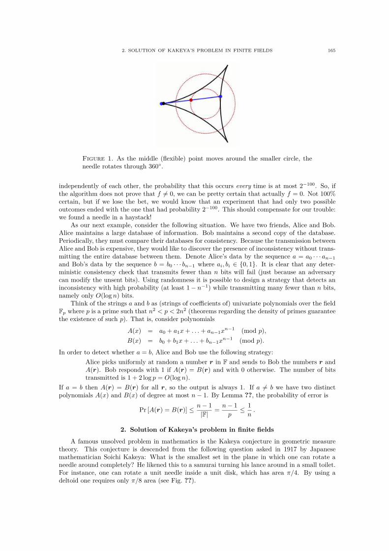
2. SOLUTION OF KAKEYA’S PROBLEM IN FINITE FIELDS 165
Figure 1. As the middle (flexible) point moves around the smaller circle, theneedle rotates through 360.
independently of each other, the probability that this occurs every time is at most 2−100. So, ifthe algorithm does not prove that f 6= 0, we can be pretty certain that actually f = 0. Not 100%certain, but if we lose the bet, we would know that an experiment that had only two possibleoutcomes ended with the one that had probability 2−100. This should compensate for our trouble:we found a needle in a haystack!
As our next example, consider the following situation. We have two friends, Alice and Bob.Alice maintains a large database of information. Bob maintains a second copy of the database.Periodically, they must compare their databases for consistency. Because the transmission betweenAlice and Bob is expensive, they would like to discover the presence of inconsistency without trans-mitting the entire database between them. Denote Alice’s data by the sequence a = a0 · · · an−1
and Bob’s data by the sequence b = b0 · · · bn−1 where ai, bi ∈ 0, 1. It is clear that any deter-ministic consistency check that transmits fewer than n bits will fail (just because an adversarycan modify the unsent bits). Using randomness it is possible to design a strategy that detects aninconsistency with high probability (at least 1 − n−1) while transmitting many fewer than n bits,namely only O(log n) bits.
Think of the strings a and b as (strings of coefficients of) univariate polynomials over the fieldFp where p is a prime such that n2 < p < 2n2 (theorems regarding the density of primes guaranteethe existence of such p). That is, consider polynomials
A(x) = a0 + a1x + . . . + an−1xn−1 (mod p),
B(x) = b0 + b1x + . . . + bn−1xn−1 (mod p).
In order to detect whether a = b, Alice and Bob use the following strategy:
Alice picks uniformly at random a number r in F and sends to Bob the numbers r andA(r). Bob responds with 1 if A(r) = B(r) and with 0 otherwise. The number of bitstransmitted is 1 + 2 log p = O(log n).
If a = b then A(r) = B(r) for all r, so the output is always 1. If a 6= b we have two distinctpolynomials A(x) and B(x) of degree at most n − 1. By Lemma ??, the probability of error is
Pr [A(r) = B(r)] ≤ n − 1
|F| =n − 1
p≤ 1
n.
2. Solution of Kakeya’s problem in finite fields
A famous unsolved problem in mathematics is the Kakeya conjecture in geometric measuretheory. This conjecture is descended from the following question asked in 1917 by Japanesemathematician Soichi Kakeya: What is the smallest set in the plane in which one can rotate aneedle around completely? He likened this to a samurai turning his lance around in a small toilet.For instance, one can rotate a unit needle inside a unit disk, which has area π/4. By using adeltoid one requires only π/8 area (see Fig. ??).
166 16. THE POLYNOMIAL METHOD
The Kakeya conjecture in more dimensions states that any subset of Rn that contains a unitline segment in every direction has Hausdorff dimension equal to n. This conjecture remains openin dimensions three and higher, and gets more difficult as the dimension increases.
To approach this question, Wolff (1999) proposed a simpler finite field analogue of the Kakeyaconjecture. If Fn is a vector space over a finite field F, define a Kakeya set to be a subset K ⊆ Fn
which contains a line in every direction, namely for any v ∈ Fn there exists a vector w ∈ Fn
such that the line w + tv : t ∈ F is contained in K; here, vector w is the origin and vector vthe direction of the line. The finite field Kakeya conjecture stated that there exists a constantc > 0 depending only on the dimension n such that every Kakeya set K ⊆ Fn has cardinality|K| ≥ c|F|n.
This finite field version of the conjecture has had a significant influence on the subject, inparticular inspiring work on the sum-product phenomenon in finite fields, which has since provedto have many applications in number theory and computer science. Modulo minor technicalities,the progress on the finite field Kakeya conjecture was, however, essentially the same as that of theoriginal “Euclidean” Kakeya conjecture.
Recently Dvir (2009) used a surprisingly simple application of the polynomial method to provethe finite field Kakeya conjecture.
Lemma 16.5. Let f ∈ F[x1, . . . , xn] be a polynomial of degree at most q − 1 over a finite fieldwith q = |F| elements. If f vanishes on a Kakeya set K, then f is the zero polynomial.
Proof. The argument is similar to that in the proof of Lemma ??. Suppose for a contradiction
that f is nonzero. We can write f =∑d
i=0 fi, where 0 ≤ d ≤ q − 1 is the degree of f and fi isthe i-th homogeneous component; thus fd is nonzero. Since f vanishes on K, d cannot be zero.Hence, fd is a nonzero polynomial.
Let v ∈ Fn\0 be an arbitrary direction. As K is a Kakeya set, K contains a line w+tv : t ∈F for some w ∈ Fn, thus f(w + tv) = 0 for all t ∈ F. The left-hand side is a polynomial gw,v(t)in t of degree at most q − 1, and must be the zero polynomial by the factor theorem, that is, allits coefficients are zero. In particular, the coefficient of td, which is fd(v), must be zero. Sincev was arbitrary, it follows that the polynomial fd(x) vanishes on all points in Fn. But sincedqn−1 ≤ (q − 1)qn−1 < qn, Lemma ?? implies that fd must be a zero polynomial.
Theorem 16.6 (Dvir 2009). Let K ⊂ Fn be a Kakeya set. Then
|K| ≥(|F | + n − 1
n
)≥ |F|n
n!.
Proof. Let q = |F| and suppose that |K| <(
n+q−1n
). Then, by Lemma ??, there exists a
nonzero polynomial f ∈ F[x1, . . . , xn] of degree at most q−1 that vanishes on K, which contradictsLemma ??.
3. Combinatorial Nullstellensatz
The following special case of Hilbert’s Nullstellensatz has found numerous applications incombinatorics.
Theorem 16.7 (Nullstellensatz). Let f ∈ F[x1, . . . , xn], and let S1, . . . , Sn be nonempty sub-sets of F. If f(x) = 0 for all x ∈ S1×· · ·×Sn, then there are polynomials h1, . . . , hn ∈ F[x1, . . . , xn]such that deg(hi) ≤ deg(f) − |Si| and
f(x1, . . . , xn) =n∑
i=1
hi(x1, . . . , xn)∏
s∈Si
(xi − s) .
Proof (due to Alon 1999). Define di = |Si| − 1 for all i, and consider polynomials
gi(xi) =∏
s∈Si
(xi − s) = xdi+1i −
di∑
j=0
aijxji .

3. COMBINATORIAL NULLSTELLENSATZ 167
Observe that if xi ∈ Si then gi(xi) = 0, that is,
(88) xdi+1i =
di∑
j=0
aijxji .
Let f be the polynomial obtained by writing f as a linear combination of monomials and replacing,repeatedly, each occurrence of xti
i (1 ≤ i ≤ n), where ti > di, by a linear combination of smaller
powers of xi, using the relations (??). The resulting polynomial f is clearly of degree at most di
in xi for each 1 ≤ i ≤ n, and is obtained from f by subtracting from it products of the form higi,where deg(hi) ≤ deg(f) − deg(gi) = deg(f) − |Si|. So,
(89) f(x) = f(x) −n∑
i=1
hi(x)gi(xi) .
Moreover, f(x) = f(x) for all x ∈ S1 × · · · × Sn, since the relations (??) hold for these valuesof x. Since, by our assumption, f(x) = 0 for all these values, we obtain that f(x) = 0 for allx ∈ S1 × · · · × Sn as well, and Exercise ?? implies that f(x) = 0 for all x ∈ Fn. Together with(??), this implies that f =
∑ni=1 higi, as desired.
Using the Nullstellensatz we can derive the following generalization of the DeMillo–Lipton–Schwartz–Zippel lemma.
Theorem 16.8 (Combinatorial Nullstellensatz). Let f(x1, . . . , xn) be a polynomial of degreed over a field F. Suppose that the coefficient of the monomial xt1
1 · · · xtnn in f is nonzero and
t1 + · · · + tn = d. If S1, . . . , Sn are finite subsets of F with |Si| ≥ ti + 1, then there are exists apoint x in S1 × · · · × Sn for which f(x) 6= 0.
Proof. We may assume that |Si| = ti + 1 for all i. Suppose the result is false, and definegi(xi) =
∏s∈Si
(xi − s). Let h1, . . . , hn be the polynomials guaranteed by the Nullstellensatz.Hence,
(90) deg(hi) ≤ deg(f) − deg(gi) = deg(f) − (ti + 1)
and f(x) =∑n
i=1 hi(x)gi(xi), that is,
f(x) =n∑
i=1
xti+1i hi(x) + (terms of degree < deg(f)) .
By assumption, the coefficient of∏n
i=1 xtii on the left-hand side is nonzero, while it is impossible
to have such a monomial on the right-hand side, a contradiction.
In a similar vein is the following result.
Theorem 16.9 (Chevalley–Warning). Let p be a prime, and f1, . . . , fm polynomials in Fp[x1, . . . , xn].If∑m
i=1 deg(fi) < n then the number of common zeros of f1, . . . , fm is divisible by p. In particular,if there is one common zero, then there is another one.
Although this theorem can be derived from the Combinatorial Nullstellensatz, we give aslightly more direct proof due to Alon (1995).
Proof. By Fermat’s Little Theorem (see Exercise ??), ap−1 ≡ 1 mod p for all a ∈ Fp, a 6= 0.Hence, the number N of common zeros of f1, . . . , fm satisfies
(91) N =∑
x1,...,xn∈Fp
m∏
j=1
(1 − fj(x1, . . . , xn)p−1) . (in Fp)
By expanding the right-hand side we get a linear combination of monomials of the formn∏
i=1
xtii with
n∑
i=1
ti ≤ (p − 1)m∑
j=1
deg(fj) < (p − 1)n.

168 16. THE POLYNOMIAL METHOD
Hence, in each such monomial there is an i with ti < p − 1. But then (see Exercise ??)∑
xi∈Fp
xtii = 0 (in Fp),
implying that the contribution of each monomial to the sum (??) is 0 modulo p, completing theproof of the theorem.
We illustrate the potential applications of the Combinatorial Nullstellensatz on several exam-ples.
3.1. The permanent lemma. Let A = (ai,j) be an n × n matrix over a field F. Thepermanent Per(A) of A is the sum
Per(A) =∑
(i1,i2,...,in)
a1,i1a2,i2
· · · an,in
of n! products, where (i1, i2, . . . , in) is a permutation of (1, 2, . . . , n).
Theorem 16.10. If Per(A) 6= 0, then for any vector b ∈ Fn, there is a subset of columns ofA whose sum differs from b in all coordinates.
This is just a special case of the following lemma for all Si = 0, 1.
Lemma 16.11 (Permanent Lemma). Let b ∈ Fn and S1, . . . , Sn be subsets of F, each of cardi-nality at least 2. If Per(A) 6= 0, then there exists a vector x ∈ S1 × · · · × Sn such that Ax differsfrom b in all coordinates.
Proof. The polynomial
f =
n∏
i=1
( n∑
j=1
aijxj − bi
)
is of degree n and the coefficient of x1x2 · · · xn in it is Per(A) 6= 0. The result now follows directlyfrom the Combinatorial Nullstellensatz with all ti = 1.
3.2. Covering cube by affine hyperplanes. An affine hyperplane is a set of vectors H =x ∈ Rn : 〈a, x〉 = b with a ∈ Rn and b ∈ R. How many such hyperplanes do we need tocover 0, 1n? If we have no further restrictions on the covering, then just two hyperplanesH0 = x ∈ Rn : 〈e1, x〉 = 0 and H1 = x ∈ Rn : 〈e1, x〉 = 1 are enough, where e1 = (1, 0, . . . , 0)is the first unit vector. But what if we, say, require that the all-0 vector 0 remains uncovered?In this case n hyperplanes Hi = x ∈ Rn : 〈ei, x〉 = 1, i = 1, . . . , n are still enough. It turns outthat this is already optimal.
Theorem 16.12. Suppose that the hyperplanes H1, H2, . . . , Hm in Rn avoid 0, but otherwisecover all 2n − 1 vertices of the cube 0, 1n. Then m ≥ n.
Proof. As 0 is not contained in Hi, we have that each hyperplane is of the form Hi = x ∈Rn : 〈ai, x〉 = 1 for some ai ∈ Rn. Assume that m < n, and consider the polynomial
f(x) =
m∏
i=1
(1 − 〈ai, x〉) −n∏
i=1
(1 − xi) .
The degree of this polynomial is clearly n (since we assumed that m < n) and the coefficientat x1 · · · xn is (−1)n+1 6= 0. When applied with Si = 0, 1 and ti = 1, the CombinatorialNullstellensatz implies that there must be a point x ∈ 0, 1n for which f(x) 6= 0. We have x 6= 0,as f(0) = 1 − 1 = 0. But then 〈ai, x〉 = 1 for some i (as x is covered by some Hi), implying thatf vanishes at this point, a contradiction.

3. COMBINATORIAL NULLSTELLENSATZ 169
3.3. Regular subgraphs. A graph is p-regular if all its vertices have degree p. The followingsufficient condition for a graph to contain a regular subgraph was derived by Alon, Friedland andKalai (1984) using the Combinatorial Nullstellensatz.
Theorem 16.13. Let G = (V, E) be a graph. Assume that G has no self-loops but multipleedges are allowed. Let p be a prime number. If G has average degree bigger than 2p − 2 andmaximum degree at most 2p − 1, then G contains a spanning p-regular subgraph.
Proof. Associate each edge e of G with a variable xe and consider the polynomial
f =∏
v∈V
[1 −
(∑
e∈E
av,exe
)p−1]−∏
e∈E
(1 − xe)
over GF (p), where av,e = 1 if v ∈ e and av,e = 0 otherwise. Note that deg(f) = |E|, since thedegree of the first product is at most (p − 1)|V | < |E|, by the assumption on the average degree2|E|/|V | of G. Moreover, the coefficient of
∏e∈E xe in f is (−1)|E|+1 6= 0.
We can therefore apply the Combinatorial Nullstellensatz with Se = 0, 1 and te = 1 for alle ∈ E and obtain a (0, 1)-vector x = (xe : e ∈ E) such that f(x) 6= 0. Consider the spanningsubgraph H consisting of all edges e ∈ E for which xe = 1. As f(0) = 0, we conclude that x 6= 0and H is non-empty. The second summand in f(x) is therefore zero and it follows from Fermat’sLittle Theorem (Exercise ??) that
∑e∈E av,exe ≡ 0 mod p for every vertex v. Therefore, in the
subgraph H all degrees are divisible by p, and since the maximum degree is smaller than 2p, allpositive degrees are precisely p, as needed.
3.4. Sum-sets. The Cauchy-Davenport Theorem, which has numerous applications in Ad-ditive Number Theory, is the following. Given two sets A and B of elements of some field F, theirsum-set is the set A + B = a + b : a ∈ A, b ∈ B.
Theorem 16.14 (Cauchy–Davenport). If p is a prime, and A, B are two non-empty subsetsof Zp, then
|A + B| ≥ minp, |A| + |B| − 1 .
We will see in Sect. ?? that this theorem is just a special case of Kneser’s theorem. Here weshow how to derive this theorem from the Combinatorial Nullstellensatz.
Proof. If |A| + |B| > p the result is trivial, since in this case for every x ∈ Zp the two sets Aand x−B intersect, implying that A+B = Zp. Assume, therefore, that |A|+ |B| ≤ p and supposethat |A+B| ≤ |A|+ |B|−2. Let C be a subset of Zp satisfying A+B ⊆ C and |C| = |A|+ |B|−2.Define a polynomial f(x, y) =
∏c∈C(x + y − c) and observe that by the definition of C,
(92) f(a, b) = 0 for all (a, b) ∈ A × B.
Put t1 = |A| − 1, t2 = |B| − 1 and note that the coefficient of xt1yt2 in f is the binomial coefficient(
t1 + t2
t1
)=
(|A| + |B| − 2
|A| − 1
)
which is nonzero in Zp, since |A| + |B| − 2 < p (see Exercise ??). We can therefore apply theCombinatorial Nullstellensatz (with n = 2, S1 = A and S2 = B) and obtain a poinr (a, b) ∈ A×Bfor which f(a, b) 6= 0, contradicting (??) and completing the proof.
The Cauchy–Davenport theorem was extended in many ways. Let us mention one importantresult in that direction. For a subset A ⊆ Zp and a natural number 1 ≤ k ≤ |A|, let sk(A) bethe number of elements b ∈ Zp that can be represented as a sum b = a1 + · · · + ak of k distinctelements of A.
Theorem 16.15 (Dias da Silva and Hamidoune 1994). If p is a prime then, for every subsetA ⊆ Zp and every 1 ≤ k ≤ |A|,
sk(A) ≥ minp, k|A| − k2 + 1 .

170 16. THE POLYNOMIAL METHOD
3.5. Zero-sum sets. Using the pigeonhole principle, one can show that any sequence a1, . . . , an
of n integers contains a non-empty consecutive subsequence ai, . . . , ai+m whose sum is divisibleby n.
To show this, make n pigeonholes labeled from 0 up to n − 1 and place the n sequences
(a1), (a1, a2), . . . , (a1, a2, . . . , an)
into the pigeonholes corresponding to the remainder when the sum is divided by n. If any of thesesequences is in the pigeonhole 0 then the sum of its numbers is divisible by n. If not, then then sequences are in the other n − 1 pigeonholes. By the pigeonhole principle some two of them,(a1, a2, . . . , ar) and (a1, a2, . . . , as) with r < s, must lie in the same pigeonhole, meaning that thesum ar+1 + ar+2 + · · · + as is divisible by n.
A question of a similar flavor is the following one. Given a natural number n, what is thesmallest N such that any sequence of N integers contains a subsequence of n (not necessarilyconsecutive) numbers whose sum is divisible by n? That is, this time we want to find a subsequenceof a given length n. The sequence 0n−11n−1 of n − 1 copies of 0 and n − 1 copies of 1 shows thatN ≥ 2n − 1. It turns out that this lower bound is also an upper bound for the sequence length N .
Theorem 16.16 (Erdős–Ginzburg–Ziv 1961). Any sequence of 2n − 1 integers contains asubsequence of cardinality n, the sum of whose elements is divisible by n.
There are several different proofs of this theorem – the interested reader can find them, aswell as some interesting extensions of this result to higher dimensions, in the paper of Alon andDubiner (1993). The original proof was based on the Cauchy–Davenport theorem.
First proof of Theorem ??. We will first prove the theorem only for the case when n = p is a primenumber, and then show how the general case reduces to it.
Let a1 ≤ a2 ≤ . . . ≤ a2p−1 be integers. If ai = ai+p−1 for some i ≤ p − 1, then ai + ai+1 +· · · + ai+p−1 = pai = 0 (in Zp) and the desired result follows. Otherwise, define Ai := ai, ai+p−1for i = 1, . . . , p − 1. By repeated application of the Cauchy-Davenport theorem, we conclude that
|A1 + A2 + · · · + Ap−1| ≥ minp, |A2 + · · · + Ap−1| + 1≥ minp, |A3 + · · · + Ap−1| + 2
· · ·≥ minp, |Ap−1| + p − 2 = p ,
and hence, every number from Zp is a sum of precisely p − 1 of the first 2p − 2 elements of oursequence. In particular, the number −a2p−1 is such a sum, supplying the required p-element subsetwhose sum is 0 in Zp.
The general case may be proved by induction on the number of primes in the prime factor-ization of n. Put n = pm where p is a prime, and let a1, . . . , a2n−1 be the given sequence. By theresult for the prime case, each subset of 2p−1 members of the sequence contains a p-element subsetwhose sum is 0 modulo p. Therefore, we can find pairwise disjoint p-element subsets I1, . . . , Iℓ of1, . . . , 2n − 1, where ∑
j∈Ii
aj ≡ 0 mod p
for each i = 1, . . . , ℓ. Moreover, ℓ ≥ 2m − 1 since otherwise the number of left elements wouldstill be 2pm − 1 − (2m − 2)p = 2p − 1, and we could choose the next subset Iℓ+1. Now define asequence b1, . . . , b2m−1 where
bi =∑
j∈Ii
aj
p
(recall that each of these sums is divisible by p). By the induction hypothesis this new sequencehas a subset bi : i ∈ J of |J | = m elements whose sum is divisible by m, and the union of thecorresponding sets aj : j ∈ Ii with i ∈ J supplies the desired n-element subset of our originalsequence, whose sum is divisible by n = pm.
Theorem ?? can also be derived using the Chevalley–Warning theorem about the zeroes ofmultivariate polynomials (see Theorem ??).

EXERCISES 171
Second proof of Theorem ?? (Alon 1995). We will prove the theorem only for a prime n = p; thegeneral case reduces to it (see the first proof of Theorem ??).
Let a1, a2, . . . , a2p−1 be integers, and consider the following system of two polynomials in 2p−1variables of degree p − 1 over Fp:
2p−1∑
i=1
aixp−1i = 0,
2p−1∑
i=1
xp−1i = 0 .
Since 2(p − 1) < 2p − 1 and x1 = x2 = · · · = x2p−1 = 0 is a common solution, Theorem ?? impliesthe existence of a nontrivial common solution (y1, . . . , y2p−1). Since p is a prime, Fermat’s LittleTheorem (see Exercise ??) tells us that xp−1 = 1 in Fp for every x ∈ Fp, x 6= 0. So, if we takeI = i : yi 6= 0 then the first equation ensures that
∑i∈I ai = 0, while the second ensures that
|I| ≡ 0 mod p, and hence, that |I| = p because |I| ≤ 2p − 1. This completes the proof of thetheorem for prime n.
Exercises
Ex 16.1. Let p ≥ 2 be a prime and consider the field Fp. From Algebra we know that there isan a ∈ Fp such that Fp \0 =
ai : i = 0, 1, . . . , p − 2
. Use this fact together with Fermat’s Little
Theorem to prove that, for every t ≤ p−2,∑
x∈Fpxt = 0 in Fp. Hint:
∑n
i=0zi = (zn+1 −1)/(z −1).
Ex 16.2 (Low local degree polynomials). Let f be a nonzero polynomial in n variables overa field F. Suppose that the maximum exponent of each of its variables in f does not exceed d.(Hence, the degree of f may be up to dn which makes the bound given by Lemma ?? trivial, if|S| ≤ n.) Show that we still have the following upper bound: For any subset S ⊆ F of size |S| ≥ d,
|x ∈ Sn : f(x) 6= 0| ≥ (|S| − d)n .
Hint: Argue by induction on n. In the induction step take a point (a1, . . . , an) ∈ Fn on which f(a1, . . . , an) 6=
0, and consider two polynomials:
f0(x1, . . . , xn−1) := f(x1, . . . , xn−1, an)
f1(xn) := f(a1, . . . , an−1, xn).
Ex 16.3. Show that the bound in Exercise ?? is the best possible. Hint: Consider the polynomialf(x1, . . . , xn) =
∏d
i=1(x1 − i) · · ·
∏d
i=1(xn − i) .
Ex 16.4. Use Exercise ?? to show the following: If S a subset of F that has d + 1 elements,then any nonzero polynomial of local degree d has a nonzero point in Sn.
Ex 16.5. Prove the following “granulated” version of the result established in Exercise ??.Let f ∈ F[x1, . . . , xn] be a polynomial, and let ti be the maximum degree of xi in f . Let Si ⊆ F
with |Si| ≥ ti. If f(x) = 0 for all n-tuples x ∈ S1 × · · · × Sn, then f(x) = 0 for all x ∈ Fn.
Ex 16.6. Let f(x1, . . . , xn) be a multivariate polynomial over a field F with the degree sequence(d1, . . . , dn), which is defined as follows: let d1 be the maximum exponent of x1 in f , and let
f1(x2, . . . , xn) be the coefficient of xd11 in f ; then, let d2 be the maximum exponent of x2 in f1,
and f2(x3, . . . , xn) be the coefficient of xd22 in f1; and so on. Suppose that f is not the zero
polynomial, and let S1, . . . , Sn ⊆ F be arbitrary subsets. For ri ∈ Si chosen independently anduniformly at random, show that
Pr [f(r1, . . . , rn) = 0] ≤ d1
|S1| +d2
|S2| + · · · +dn
|Sn| .
Ex 16.7. (R. Freivalds 1977). Suppose that somebody gives us three n × n matrices A, B, Cwith real entries and claims that C = A · B. We are too busy to verify this claim exactly and dothe following. We take a random vector r of length n whose entries are integers chosen uniformlyfrom the interval 0, 1, . . . , N −1, and check whether A·(B ·r) = C ·r. If this is true we accept theclaim, otherwise we reject it. How large must N be set to make the probability of false acceptancesmaller than 1/100? Hint: Consider the matrix X = A · B − C. If C 6= A · B then X has a row x 6= 0.

172 16. THE POLYNOMIAL METHOD
Take a scalar product of this row with the random vector r, observe that Pr [X · r = 0] ≤ Pr [x · r = 0],and apply Exercise ??.

CHAPTER 17
Combinatorics of Codes
In this chapter we will discuss some extremal properties of error-correcting codes. We willalso use expander graphs to construct very easily decodable codes.
1. Error-correcting codes
Error-correcting codes enable one to store or transmit a message in such a way that one canlater recover the message even if it is partially corrupted, that is, up to some number t of bits areflipped by noise. Messages are strings of some fixed length k over some alphabet A. In order tobe able to recover corrupted messages, we encode our messages by strings of length n > k over A(or some other alphabet). That is, we take a particular subset C ⊆ An (called a code) and assignto each message w its own codeword x = xw ∈ C.
During the transmission some bits may be flipped (by noise, by an adversary or whatever).So, the receiver is presented with a corrupted version x′ ∈ An of the original codeword x ∈ C. Thereceiver knows the set of all codewords C, as well as the encoding algorithm. He also knows thatthe received vector x′ can differ from the original x codeword in at most t bits. What conditionsmust the code C fulfill in order that we may recover the original codeword x?
Here the notion of Hamming distance comes into the play. The Hamming distance dist(x, y)between two strings x and y of the same length is just the number of positions in which thesetwo strings differ. The minimum distance, dist(C), of a subset C ⊆ An is the minimal Hammingdistance dist(C) between any pair of distinct strings in C.
The key observation is that, if dist(C) ≥ 2t + 1, then the receiver can (at least in principle)reconstruct the original codeword x from the received, possibly corrupted vector x′. The point isthat x is the only codeword in the Hamming ball Bt(x
′) = y ∈ An : dist(x′, y) ≤ t of radius taround the corrupted vector x′: were another codeword y ∈ C also to lie in Bt(x
′) then we wouldhave that dist(x, y) ≤ dist(x, x′) + dist(x′, y) ≤ 2t, contradicting dist(C) ≥ 2t + 1.
Thus, the larger dist(C) is, the better, the more errors we can correct. Another importantparameter of codes is their size, that is, the total number of codewords the sender has in hisdisposal. The larger |C| is, the better, the more distinct messages can be encoded.
Of course, if each two codewords must differ in many positions, then we cannot have manycodewords. In particular, we have the following general upper bound.
Theorem 17.1 (Singleton bound). If C ⊆ An and d = dist(C) then
|C| ≤ |A|n−d+1 .
Proof. Clearly, all codewords in C are distinct. If we delete the first d − 1 letters of eachcodeword, then all resulting codewords must still be pairwise different, since all original codewordsin C have Hamming distance at least d from each other. Thus the size of the code remainsunchanged. The newly obtained codewords each have length n − (d − 1) = n − d + 1 and thusthere can be at most |A|n−d+1 of them.
We now construct codes achieving this upper bound. These codes were proposed by Reed andSolomon (1960). Let k ≤ n ≤ q, where q is a power of a prime. As our alphabet we take a fieldA := Fq with |A| = q elements. Fix n distinct elements α1, . . . , αn of Fq; here we need that q ≥ n.Messages are strings w = (w1, . . . , wk) of elements of Fq. We identify each such message with thepolynomial pw(z) = w1 + w2z + · · · + wkzk−1 of degree at most k − 1 over Fq. The codeword of
173

174 17. COMBINATORICS OF CODES
the message w is then the string xw =(pw(α1), . . . , pw(αn)
)of the evaluation of the polynomial
pw(z) at all n fixed points. Let C = xw : w ∈ Ak be the resulting code.Since, by the factor theorem, no two distinct polynomials of degree at most k − 1 can agree
on k or more points, we have that dist(C) ≥ n − k + 1. In this way we have constructed a codeC ⊆ An of minimum distance d = n − k + 1 and size |C| = |A|k = |A|n−d+1.
Thus, Reed–Solomon codes meet the Singleton bound. The drawback of these codes is thecondition that q ≥ n. The problem is that we need each coordinate of a codeword to correspondto a distinct element of Fq.
There are different ways to reduce the alphabet size. A trivial one is just to encode all qelements of Fq by binary strings of length ⌈log2 q⌉. Then one obtains a binary code C ⊆ 0, 1n
with codeword length n = q⌈log2 q⌉, size |C| ≥ qk and minimum distance dist(C) ≥ n − k + 1.Although binary codes with better parameters are known, the binary Reed–Solomon codes areone of the most commonly used codes in practical applications. In particular, they are used tostore information, music, and video on compact discs (CDs) and digital video discs (DVDs).
Another way to reduce the field size q is to use multivariate polynomials. In particular, usingbivariate polynomials, q only needs to be
√n. For this, let the message length be k = (t/2 + 1)2
and look at messages w ∈ Fkq as (t/2 + 1) × (t/2 + 1) matrices w = (wij) over Fq. Each such
message determines a bivariate polynomial
pw(y, z) =
t/2∑
i,j=0
wijyizj
of degree at most t over Fq. The codeword of the message w is then the string xw =(pw(α, β) : α, β ∈
Fq
)of the values of the polynomial pw on all points of Fq ×Fq. Thus we only require that q2 ≥ n,
instead of q ≥ n. As before, the resulting code C = xw : w ∈ Fkq has |C| = qk codewords. Fur-
ther, since the polynomials are of degree at most t, the DeMillo–Lipton–Schwartz–Zippel lemmaimplies that dist(C) ≥ (1 − t/q)n.
Extending this idea to multivariate polynomials, we arrive at Reed–Muller codes. In this casewe identify messages with polynomials of degree at most t in m variables z1, . . . , zm. The codewordlength in this case is n = qm. The number of codewords is the number of monomials of degreeat most ℓ in m variables which, by Exercise ??, is equal to
(m+t
t
). Finally, the DeMillo–Lipton–
Schwartz–Zippel lemma implies that dist(C) ≥ (1 − t/q)n.A binary Reed–Muller code C ⊆ 0, 1n corresponds to the case when q = 2 and t = 1.
That is, messages are multilinear polynomials in m variables over F2. In this case we have that|C| =
(m+1
1
)= m+1 codewords of length n = 2m, and the minimum distance is at least n/2. Note
that these codes have exactly the same parameters as Hadamard codes constructed in Sect. ??(see Theorem ??).
2. Bounds on code size
If the minimum distance d is given, how large can |C| then be? To answer this question, letVol(n, r) be the number of vectors in the Hamming ball Br(0) of radius r around the all-0 vector.Since this ball consists of all vectors with at most r ones, we have that
2n·H(r/n)−O(log n) ≤ Vol(n, r) =
r∑
i=0
(n
i
)≤ 2n·H(r/n) ,
where H(x) = −x log2 x− (1−x) log2(1−x) is the binary entropy function; the estimates in termsof this function are proved in Exercises ?? and ??.
Theorem 17.2 (Gilbert–Varshamov and Hamming bounds). Codes C ⊆ 0, 1n of minimaldistance d and size
(93) |C| ≥ 2n
Vol(n, d)

2. BOUNDS ON CODE SIZE 175
exist, and for any such code with d ≥ 2t + 1, we have that
(94) |C| ≤ 2n
Vol(n, t).
The lower bound (??) is known as the Gilbert–Varshamov bound, and the upper bound (??)as the Hamming bound.
Proof. The lower bound can be obtained by a simple algorithm: Pick any vector x ∈ 0, 1n,include it in C, remove the whole ball Bd(x) around this vector, and do the same in the set of theremaining vectors.
To show the upper bound, let C ⊆ 0, 1n be a code of minimum distance d ≥ 2t + 1. Draw aball of radius t around each of the vectors in C. If the balls around some two codewords were tointersect, then the Hamming distance between these two codewords would be at most 2t < d, acontradiction. Therefore, the balls are disjoint, and their number is limited by the overall volumedivided by the volume of each ball.
More upper bounds on the size of codes can be obtained using linear algebra. For this, wefirst embed the Hamming spaces (binary cubes) into Euclidean spaces over the reals. We embeda vector v ∈ 0, 1n as the vector xv ∈ Rn by changing its coordinates by the rules 0 7→ +1 and1 7→ −1. Thus, xv is a ±1 vector.
The following relations between the Hamming and Euclidean distances are easy to verify (dothis!).
Proposition 17.3. For u, v ∈ 0, 1n with Hamming distance dist(u, v) = d, we have that〈xu, xv〉 = n − 2d, ‖xu‖2 = n and ‖xu − xv‖2 = 4d.
Our first goal is to prove a geometric fact: In n dimensions there exist at most 2n vectors thatpairwise subtend an angle of at least π/2 at the origin (that is, their pairwise scalar products are≤ 0).
Lemma 17.4 (Obtuse angles).
(i) Let x1, . . . , xm be vectors in Rn, and α a positive number. If ‖xi‖ = 1 and 〈xi, xj〉 ≤ −α forall i 6= j, then m ≤ 1 + α−1.
(ii) If y, x1, . . . , xm ∈ Rn satisfy 〈xi, xj〉 ≤ 0 for all i 6= j, while 〈y, xi〉 > 0 for all i, then m ≤ n.(iii) If x1, . . . , xm ∈ Rn are nonzero and satisfy 〈xi, xj〉 ≤ 0 for all i 6= j, then m ≤ 2n.
Proof. (i) Let z = x1 + · · · + xm. On the one hand, we have 〈z, z〉 ≥ 0. On the other hand,we have
〈z, z〉 =
m∑
i=1
〈xi, xi〉 +
m∑
i6=j∈[m]
〈xi, xj〉
≤ m · 1 + m(m − 1) · (−α)
= m(1 − α(m − 1)) .
Putting the two inequalities together, we have 1 − α(m − 1) ≥ 0, implying m ≤ 1 + 1/α.(ii) Assume for the sake of contradiction that m ≥ n + 1. Then there must exist a linearly
dependent set of vectors among the xi’s. Specifically, there exist disjoint sets S, T ⊆ [m] andpositive λi, for i ∈ S ∪ T , such that
∑i∈S λixi =
∑j∈T λjxj . It is not necessary that both S and
T be non-empty, but at least one, say S, is non-empty. Let z =∑
i∈S λixi =∑
j∈T λjxj . Ouranalysis divides into two cases depending on whether or not z = 0.
If z 6= 0, then we obtain a contradiction as follows:
0 < 〈z, z〉 =⟨∑
i∈S
λixi,∑
j∈T
λjxj
⟩=∑
i∈S
∑
j∈T
λiλj〈xi, xj〉 ≤ 0 ,
where the last inequality uses the fact that S and T are disjoint and so 〈xi, xj〉 ≤ 0 for every i ∈ Sand j ∈ T .
176 17. COMBINATORICS OF CODES
If z = 0, then we use the existence of the vector y to obtain a contradiction as follows:
0 = 〈y, 0〉 = 〈y, z〉 =⟨
y,∑
i∈S
λixi
⟩=∑
i∈S
λi〈y, xi〉 > 0 .
The last inequality is strict since S 6= ∅, λi > 0 and 〈y, xi〉 > 0.(iii) Pick a vector y such that 〈y, xi〉 6= 0 for all i ∈ [m]. At least half of the vectors xi must
have a positive scalar product with either y or −y. Assume w.l.o.g. that x1, . . . , x⌈m/2⌉ have apositive scalar product with y. Applying part (ii) to these vectors and y, we get ⌈m/2⌉ ≤ n.
Theorem 17.5 (Plotkin bound). If C ⊆ 0, 1n and d = dist(C), then
|C| ≤ d2n−2d+2 .
Proof. We first prove the following claim: If d ≥ n/2 then |C| ≤ 2n. Let c1, . . . , cm be thecodewords of C, and let x1, . . . , xm be their ±1 versions. Since d ≥ n/2, Proposition ?? impliesthat 〈xi, xj〉 ≤ n − 2d ≤ 0 for all i 6= j, and Lemma ??(iii) implies that m ≤ 2n, as claimed.
To derive the theorem from this claim, write n = 2d + k. By restricting C to the mostcommonly occurring pattern in the first k coordinates and deleting these coordinates, we get a setC ′ ⊆ 0, 12d of size |C ′| ≥ |C|/2k and minimum distance d. By the claim we just proved, thisimplies
|C| ≤ |C ′| · 2k ≤ 2(2d) · 2k ≤ d2k+2 = d2n−2d+2 .
One of the best upper bounds is the following one.
Theorem 17.6 (Johnson bound). If C ⊆ 0, 1n and dist(C) ≥ δn then
|C| ≤ n2n
Vol(n, τn − 1)≤ 2(1−H(τ))n ,
where τ = (1 −√
1 − 2δ)/2.
Proof. For a set of strings C ⊆ 0, 1n and a positive integer t, let degt(C) denote the maximumnumber of vectors from C in a Hamming ball of radius t. If dist(C) ≥ 2t + 1, then clearlydegt(C) ≤ 1. Hence, the following claim generalizes the Hamming bound (??).
Claim 17.7. For every subset C ⊆ 0, 1n, and every positive integer t, we have that
|C| ≤ 2n · degt(C)
Vol(n, t).
Proof of Claim ??. If we consider the balls of radius t around the strings in C, then anystring in 0, 1n is considered at most degt(C) times. Thus the sum of volumes of these balls isat most 2n · degt(C).
Now let c1, . . . , cm be the codewords of a code of minimum distance d = δn that are within aHamming ball of radius t = τn − 1 from some string b ∈ 0, 1n. By the claim above, it is enoughto show that m ≤ n.
For i ∈ [m], let xi be the ±1 version of ci scaled (i.e., multiplied) by 1/√
n, and let y be the±1 version of b scaled by 1/
√n. We scale the vectors just to achieve ‖xi‖ = 1 and ‖y‖ = 1. By
Proposition ??, we have that 〈xi, xj〉 ≤ 1 − 2δ for all i 6= j, and 〈y, xi〉 > 1 − 2τ for all i. Note thesyntactic similarity of these conditions to those in Part (ii) of Lemma ??. In fact we can reduceour problem to exactly this case. We will just shift our origin to a new vector v := αy so thatfrom this vector, the vectors xi mutually subtend an angle at least π/2.
Claim 17.8. There exists an 0 ≤ α < 1 such that for v := αy we have that 〈xi −v, xj −v〉 ≤ 0and 〈xi − v, y − v〉 > 0 for all i 6= j.
Together with Lemma ??(ii), this claim gives the desired upper bound m ≤ n. So, it remainsto prove the claim.
3. LINEAR CODES 177
Proof of Claim ??. We will not specify α yet, only that it will lie in the interval 0 ≤ α < 1.Since 〈xi, xj〉 ≤ 1 − 2δ and 〈y, xi〉 > 1 − 2τ , for such an α we have that
〈xi − αy, xj − αy〉 ≤ 1 − 2δ − 2α(1 − 2τ) + α2 = (1 − α)2 + 4ατ − 2δ .
The right-hand side is minimized at α := 1 − 2τ , and for this setting, it is equal to 4τ − 4τ2 − 2δ.Since τ = (1 −
√1 − 2δ)/2 (by our choice), we have that (1 − 2τ)2 = 1 − 2δ, which in turn implies
2δ = 1 − (1 − 2τ)2 = 4τ − 4τ2, and hence, 4τ − 4τ2 − 2δ = 0. We conclude that for this setting〈xi − αy, xj − αy〉 ≤ 0, as desired. Since 〈y, xi〉 > 1 − 2τ , for the same setting α = 1 − 2τ , we alsohave that
〈xi − αy, (1 − α)y〉 = (1 − α)〈xi, y〉 − α(1 − α)‖y‖2 = (1 − α)[〈xi, y〉 − α] > 0 ,
which yields the other part of the claim.
3. Linear codes
If C ⊆ 0, 1n forms a linear subspace over F2, then C is called a linear code. Being a linearsubspace over F2 just means that x⊕y ∈ C for all x, y ∈ C. It can easily be verified (do this!) thatthe Reed–Solomon and Reed-Muller codes we constructed above using polynomials are linear.
If C has dimension k, then |C| = 2k and the code C can be described using its generatormatrix. This is a k × n matrix G whose rows form a basis of C; hence, C = u⊤G : u ∈ Fk
2.Dually, the parity-check matrix of C is the generator matrix H of the dual code
C⊥ = y ∈ Fn2 : 〈x, y〉 = 0 for all x ∈ C .
That is, H is an (n − k) × n matrix H such that C = x : Hx = 0.A general scenario is then as follows. Messages we want to send to our friend are vectors u
in Fk2 . We encode such a message as a vector x = u⊤G and send it. Our friend receives some
vector x′ which may differ from x on up to t bits. He then searches for the unique vector x suchthat Hx = 0 and dist(x, x′) ≤ t. In fact, it is enough to search for a unique vector a ∈ Bt(0) forwhich Ha = Hx′; then x = x′ ⊕ a because H(x′ ⊕ a) = 0. This decoding procedure is known assyndrome decoding, because a gives us the locations of the errors.
The first important property of a linear code C (not shared by arbitrary codes) is the followingfact. By a weight |x| of a vector x we mean the number of its nonzero coordinates.
Proposition 17.9. Every linear code has minimum distance equal to the minimum weight ofits nonzero codewords.
Proof. Let C ⊆ 0, 1n be a linear code, and let w(C) be the minimum weight of a nonzerocodeword. Take vectors x 6= y and z 6= 0 in C such that dist(x, y) = dist(C) and |z| = w(C).Then dist(C) = |x ⊕ y| ≥ w(C), since x ⊕ y belongs to C. On the other hand, we have thatw(C) = |z| = dist(z, 0) ≥ dist(C), since vector 0 belongs to C.
The next important property of linear codes is that their minimum distance is related to linearindependence of the columns of their parity-check matrices.
Theorem 17.10. Let C be a linear code with parity-check matrix H. Then the minimumdistance of C is d if and only if every set of d − 1 columns of H are linearly independent but somed columns are linearly dependent.
Proof. We already know that the minimum distance of C is equal to the smallest of theweights of the nonzero codewords. On the other hand, Hx = 0 for a nonzero vector x 6= 0 meansthat the columns of H corresponding to the 1-positions of x are linearly dependent. Thus, ifd = dist(C) then some d columns of H must be linearly dependent (since C contains a codewordof weight d), and no d − 1 columns can be linearly dependent, for otherwise C would contain acodeword of weight smaller than d.
This fact can be used to show that linear codes with minimum distance d and about 2n/nd
codewords exist.

178 17. COMBINATORICS OF CODES
Theorem 17.11. A linear code C ⊆ 0, 1n of dimension k and minimum distance d existsprovided that
(95)d−2∑
i=0
(n − 1
i
)< 2n−k .
That is, linear codes of size |C| ≥ 2n/Vol(n − 1, d − 2) exist. This is almost the same boundas for arbitrary codes given in (??).
Proof. We shall construct an (n − k) × n matrix H over F2 with the property that no d − 1columns are linearly dependent. Put r = n − k. Choose the first column of H to be any nonzeror-tuple in Fr
2 Then choose the second column to be any nonzero r-tuple different from the first.Continue choosing successive columns so that each new column is not a linear combination of anyd − 2 or fewer previous columns. When we come to try to choose the i-th column, those r-tuples
not available to us will be the N(i) =∑d−2
j=0
(i−1
j
)linear combinations of d − 2 or fewer columns
from the i − 1 columns already chosen. Not all of these linear combinations need be distinctvectors, but even in the worst case, where they are distinct, provided N(i) is less than the totalnumber 2r of all r-tuples, then an i-th column can be added to the matrix. Thus, since (??) holds,we will reach a matrix H having n columns, as required.
We are not going to sink into different constructions of explicit codes: there are so manyof them. We just mention that so-called BCH codes, constructed by Bose, Chaudhuri and Hoc-quenghem, are linear codes with quite good parameters: for every integers m ≥ 3 and t < 2m−1
there is an explicit linear code C ⊆ 0, 1n with n = 2m − 1, |C| ≥ 2n−mt and dist(C) ≥ 2t + 1.See the book by MacWilliams and Sloane (1977) for more constructions.
4. Universal sets from linear codes
Recall that a set of 0-1 strings A ⊆ 0, 1n is (n, k)-universal if, for any subset S ⊆ [n] of|S| = k coordinates, the projection of A onto the indices in S contains all possible 2k configurations.
In Sect. ?? we have shown how to construct explicit (n, k)-universal sets of size about n, whenk ≤ (log n)/3. This construction was based on Paley graphs. Here we will show how to constructsuch sets of size nO(k) for arbitrary k. The construction is based on some elementary propertiesof linear codes.
We already know that the minimal distance of C coincides with the minimum weight of (i.e.,the number of 1s in) a nonzero vector from C. This simple property of linear codes implies thattheir duals are universal.
Proposition 17.12. If C is a linear code of length n and its dual C⊥ has minimal distanceat least k + 1 then the code itself is (n, k)-universal.
Since a parity-check matrix of C is a generator matrix of C⊥, an equivalent condition on C isthat any k columns of its generator matrix must be linearly independent.
Proof. Take a set S ⊆ 1, . . . , n with |S| = k. The set of all projections of vectors in Conto S forms a linear subspace in 0, 1|S| of dimension k. If this subspace were proper then, byProposition ??, some nonzero vector x, whose support i : xi 6= 0 lies in S, would belong to C⊥,implying that dist(C⊥) ≤ |S| = k, which contradicts our assumption.
It is known (see, for example, MacWilliams and Sloane (1977)) that the dual of a binary BCHcode of minimal distance k has only O(n⌊k/2⌋) vectors. By Proposition ??, these codes give usexplicit (n, k)-universal sets consisting of only so many vectors.
One of the best known explicit constructions of (n, k)-universal sets of size only 2O(k4) log n isdue to Alon (1986a). His construction is based on a Justesen-type code constructed by Friedman(1984).

5. SPANNING DIAMETER 179
5. Spanning diameter
So far, we have used algebraic properties of linear spaces to derive some results in combina-torics. But these spaces themselves have some interesting combinatorial properties as well.
Let A be a set of vectors in 0, 1n and consider its span over the field F2. Each vector inspan A is a linear combination of some vectors from A. Some of these combinations may be short,but some may be long. Given A, we are interested in the smallest number k such that every vectorfrom span A is a sum (over F2) of at most k vectors of A; we call this k the spanning diameter ofA.
Of course, the answer depends on how large the span is, compared with the set itself. It is easyto show that if |A| > |span A|/2, then the spanning diameter of A is at most 2 (see Exercise ??).But what if A is a smaller fraction of span A, say, an α-fraction for some α > 1/4? It turns outthat then the spanning diameter does not exceed 4. In general, we have the following upper boundon k.
Theorem 17.13. Let A ⊆ 0, 1n. If |A| ≥ α · |span A| for some 0 < α ≤ 1, then every vectorfrom span A is a sum of at most k vectors from A, where k is the maximal number satisfying theinequality
(96) k − ⌊log2 k⌋ − 1 ≤ log2(1/α)
Theorem ?? can be derived from known bounds on the covering radius of binary linear codes(see, for example, Cohen et al. 1997; Theorem 8.1.21). Here we present a direct argument due toPavel Pudlák.
Proof. Take a maximal set of vectors a1, a2, . . . , ak in A such that the vector
(97) v = a1 + a2 + · · · + ak,
cannot be represented as a sum of fewer than k vectors from A. (Here and throughout the proofall the sums are over F2.) Our goal is to show that then k must satisfy (??). Since α ≤ 1, thecases k = 1 and k = 2 are trivial. So, assume that k ≥ 3.
We will need a lower bound on the size of distance-3 codes. Such codes can be obtained byshortening the Hamming code (see, for example, MacWilliams and Sloane (1977)); Exercise ??sketches a way to do this.
Claim 17.14. There exists a set C ⊆ Fk2 such that any two vectors of C differ in at least 3
coordinates and log2 |C| ≥ k − ⌊log2 k⌋ − 1.
Fix such a set C, and let B be the set of all those vectors b from span A which can berepresented in the form b = c1a1 + c2a2 + · · · + ckak for c = (c1, . . . , ck) ∈ C. The key point isthat all the translates
b + A := b + a : a ∈ A,
with b ∈ B, are mutually disjoint.
Claim 17.15. For every pair b, b′ of distinct vectors from B, the sets b + A and b′ + A aredisjoint.
Proof of Claim ??. Suppose not. Then for some a, a′ ∈ A we have b + a = b′ + a′, and hence,a+a′ = b+b′. Let c, c′ be the vectors from C for which b = c1a1+· · ·+ckak and b′ = c′
1a1+· · ·+c′kak.
Then
a + a′ = b + b′ = (c1 + c′1)a1 + (c2 + c′
2)a2 + · · · + (ck + c′k)ak.
Since vectors c and c′ differ in at least three coordinates, we have on the right-hand side the sum ofat least three vectors, say ai1 + · · · + ail , with l ≥ 3. But then in the equation (??) we can replacethese three (or more) vectors ai1 , . . . , ail by two vectors a, a′, which contradicts the minimalityof k.
The same argument also implies that no two distinct vectors c, c′ ∈ C can lead to one and thesame vector b ∈ B, that is, c 6= c′ ∈ C implies
∑i cia
i 6= ∑i c′ia
i. This means that |B| = |C|.

180 17. COMBINATORICS OF CODES
[rgb]0,0,0
.
.
.
..........................
[rgb]0,0,0
.
.
.
..........................
[rgb]0,0,0
.
.
.
..........................
[rgb]0,0,0
.
.
.
..........................
[rgb]0,0,0
.
.
.
..........................
[rgb]0,0,0
.
.
.
..........................
[rgb]0,0,0
...........................................................................................................................................
[rgb]0,0,0
.............................................................................................................................................................................................
[rgb]0,0,0
.....................................................................................................................................
[rgb]0,0,0
.........................................................................................................................................................
[rgb]0,0,00
[rgb]0,0,0R
[rgb]0,0,0
[rgb]0,0,0L
[rgb]0,0,0[rgb]0,0,01
[rgb]0,0,01
[rgb]0,0,00
[rgb]0,0,0
...............................................................................................................................................
Figure 1. Vertex v2 is satisfied whereas v1 is not satisfied by the vector x = (1010).
This, together with Claim ??, implies
|A| · |C| = |A| · |B| =∑
b∈B
|b + A| = |⋃
b∈B
(b + A)| ≤ |span A|.
Hence, log2 |C| ≤ log2(1/α) which, together with Claim ??, yields the desired upper bound (??)on k.
6. Expander codes
If C ⊆ 0, 1n is a linear code with a k ×n generator matrix G, then the encoding of messagesw ∈ 0, 1k is very easy: just encode w by the codeword x = w⊤G. However, the decoding—thatis, given a vector y ∈ 0, 1n find a codeword x ∈ C closest to y—is in general linear codes a verydifficult problem (it is “NP-hard”).
We now show how using expander graphs one can construct linear codes for which decodingis almost trivial—it can be done in linear time! Moreover, if the expansion of the graph is goodenough then the resulting codes achieve very good rate (log2 |C|)/n and minimal distance (boththese parameters are then absolute positive constants).
Let G = (L ∪ R, E) be a bipartite graph with |L| = n, |R| = m and E ⊆ L × R. Each suchgraph defines a linear code C ⊆ 0, 1n as follows. Associate with each vertex u ∈ L a booleanvariable xu. Given a vector x ∈ 0, 1n, say that a vertex v ∈ R is satisfied by this vector if
∑
u∈Γ(v)
xu mod 2 = 0 ,
where Γ(v) = u ∈ L : uv ∈ E is the set of all neighbors of v on the left side (see Fig. ??). Thecode defined by the graph G is the set of vectors
C = x ∈ 0, 1n : all vertices in R are satisfied by x .
That is, C is just the set of all solutions of m linear equations in n variables. Therefore, C islinear and |C| ≥ 2n−m.
Let dist(C) be the minimal Hamming distance between two different vectors in C. A graphG = (L∪R, E) is left d-regular if each vertex in L has degree d. Such a graph is an (α, c)-expanderif every subset I ⊆ L with |I| ≤ αn has |Γ(I)| > c|I| neighbors on the right side.
Lemma 17.16. If C ⊆ 0, 1n is a code of a left d-regular (α, c)-expander with c > d/2, then
dist(C) > αn .
Proof. Assume that dist(C) ≤ αn. Then C must contain a vector x with at most αn ones.Hence, if we take the set I = u ∈ L : xu = 1, then |I| ≤ dist(C) ≤ αn. Since G is an(α, d/2)-expander, this implies |Γ(I)| > d|I|/2.
We claim that there must exist a vertex v0 ∈ Γ(I) with exactly one neighbor in I, that is,|Γ(v0) ∩ I| = 1. Indeed, otherwise every vertex v ∈ Γ(I) would have at least two neighbors in I.Therefore the number of edges leaving I would be at least 2·Γ(I) > 2·(d|I|/2) = d|I|, contradictingthe left d-regularity of G.
6. EXPANDER CODES 181
Since xu = 0 for all u 6∈ I, this implies that exactly one of the bits xu of x with u ∈ Γ(v0)is equal to 1. So,
∑u∈Γ(v0) xu = 1, and the vertex v0 cannot be satisfied by the vector x, a
contradiction with x ∈ C.
By Lemma ??, expander codes can correct relatively many errors, up to αn/2. Much moreimportant, however, is that the decoding algorithm for such codes is very efficient. The decodingproblem is the following one: given a vector y ∈ 0, 1n of Hamming distance ≤ αn/2 from some(unknown) codeword x ∈ C, find this codeword x. The decoding algorithm for expander codes isamazingly simple:
While there exists a variable such that most of its neighbors are not satisfied by thecurrent vector, flip it.
Lemma 17.17 (Sipser–Spielman 1996). If C is a code of a left d-regular (α, c)-expander withc > 3
4 d, then the algorithm solves the decoding problem in a linear number of steps.
Proof. Let y ∈ 0, 1n be a vector of Hamming distance ≤ αn/2 from some (unknown)codeword x ∈ C. Our goal is to find this codeword x. Let
I = u ∈ L : yu 6= xube the set of errors in y. If I is empty, we are done. Otherwise, assume that |I| ≤ αn. We needthis assumption to guarantee the expansion, and we will prove later that this assumption holdsthroughout the running of the algorithm.
Partition the set Γ(I) = S ∪ U into the set S of neighbors satisfied by y and the set U ofneighbors not satisfied by y. Since c > 3d/4, we have that
(98) |U | + |S| = |Γ(I)| > 34d|I| .
Now, count the edges between I and Γ(I). At least |U | of these edges must leave U . Moreover, atleast 2|S| of them must leave S because every vertex v ∈ S must have at least two neighbors inI: If v had only one such neighbor, then y would not satisfy the vertex v since y 6= x, x satisfiesv and y coincides with x outside I. Since the total number of edges between I and Γ(I) is d|I|,this implies |U | + 2|S| ≤ d|I|. Combining this with (??) we get that
d|I| − |U | ≥ 2|S| > 2 ( 34d|I| − |U |)
and therefore
(99) |U | > 12d|I| .
So, more than d|I|/2 neighbors of the |I| vertices in I are unsatisfied. Therefore there is a variablein I that has more than d/2 unsatisfied neighbors. We have therefore shown the following claim:
If I 6= ∅ and |I| ≤ αn then there is a variable with > d/2 unsatisfied neighbors.
This implies that as long as there are errors and |I| ≤ αn holds, some variable will be flippedby the algorithm. Since we flip a vertex with more unsatisfied neighbors than satisfied ones, |U |decreases with every step (flipping xu can only affect the satisfiability of neighbors of u). Wededuce that if the distance |I| of the actual vector y from x does not exceed αn/2 throughout therun of the algorithm, then the algorithm will halt with the codeword x after a linear number ofiterations.
To show that |I| can never exceed αn, recall that |I| ≤ αn/2, and hence,
(100) |U | ≤ |Γ(I)| ≤ 12αdn
hold in the beginning. Moreover, |U | decreases after each iteration. Hence, if at some step we hadthat |I| > αn, then (??) would imply |U | > αdn/2, contradicting (??).
In general, every linear code C ⊆ 0, 1n is defined by its parity-check matrix H such thatx ∈ C iff Hx = 0. Note that, if C is a code defined by a bipartite graph G, then H is just thetranspose of the adjacency matrix of G. If G is left d-regular, then every row of H has exactly dones. If G is an (α, c)-expander, then every subset I of |I| ≤ αn columns of H has ones in at leastc|I| rows. The decoding algorithm above is, given a vector y ∈ 0, 1n such that Hy 6= 0, to flipits i-th bit provided that vector H(y ⊕ ei) has fewer ones than vector Hy.

182 17. COMBINATORICS OF CODES
7. Expansion of random graphs
Explicit constructions of bipartite left d-regular (α, c)-expanders with α = Ω(1) and c > 3d/4are known. These constructions are however too involved to be presented here. Instead of that,we will show that random bipartite left-regular graphs have good expansion properties.
Let d ≥ 3 be a constant. We construct a random bipartite left d-regular n × n graph Gn,d =(L∪R, E) as follows: For each vertex u ∈ L choose its d neighbors independently at random, eachwith the same probability 1/n. The graph obtained may have multi-edges, that is, some pairs ofvertices may be joined by several edges.
Theorem 17.18. For every constant d ≥ 3, there is a constant α > 0 such that for allsufficiently large n, the graph Gn,d is an (α, d − 2) expander with probability at least 1/2.
Proof. Set (with foresight) α := 1/(e3d4). Fix any s ≤ αn, and take any set S ⊆ L of size|S| = s. We want to upper bound the probability that S does not expand by d − 2. This meansthat the ds neighbors (including multiplicities) of the vertices in S hit fewer than (d − 2)s distinctvertices on the right side, that is, some 2s of these ds neighbors land on previously picked vertices.Each neighbor lands on a previously picked vertex with probability at most ds/n, so
Pr [S does not expand by (d − 2)] ≤(
ds
2s
)(ds
n
)2s
.
By the union bound, the probability that at least one subset S of size s does not expand by (d−2)is at most
(n
s
)(ds
2s
)(ds
n
)2s
≤(
en
s
)s(eds
2s
)2s(ds
n
)2s
≤(
e3d4
4n
)s
≤(
1
4
)s
,
by the choice of α. Thus, the probability that some set S of size |S| ≤ αn does not expand by(d − 2) does not exceed
αn∑
s=1
4−s <
∞∑
s=1
4−s <1
2.
Hence, the graph Gn,d is an (α, d − 2) expander with probability at least 1/2.
Exercises
Ex 17.1. Prove the following stronger version of Proposition ??. Let C be a linear code oflength n and minimal distance at least k + 1 and let C⊥ be its dual. Then for every subset Sof l ≤ k coordinates, every 0-1 string of length l appears as a projection of C⊥ onto S the samenumber of times. Hint: Take a matrix whose rows form a basis of C⊥, observe that every k columns ofthis matrix are linearly independent and use Proposition ??.
Ex 17.2. Let V ⊆ Fn2 be a subspace of dimension d. Show that |V | = 2d.
Ex 17.3. Let A ⊆ Fn2 and suppose that |A| > |span A|/2. Prove that every vector in span A
is the sum of at most 2 vectors from A. Hint: Show that, for every v ∈ span A, the set A ∩ (v + A) hasat least one vector.
Ex 17.4. Theorem ?? gives an upper bound on the spanning diameter of sets A in termsof their density α = |A|/|span A|. Show that for infinitely many values of k, the bound (??) isoptimal, that is, exhibit sets A whose spanning diameter is the maximal number satisfying (??).Hint: Consider the set consisting of the all-0 vector and k vectors with precisely one 1; its density isα = (k + 1)/2k.
Ex 17.5. (Hamming code). Let r be a positive integer, and let k = 2r − 1. Consider the r × kmatrix H whose columns are all the distinct nonzero vectors of 0, 1r. Let C ⊆ Fk
2 be the set ofvectors, each of which is orthogonal (over F2) to all the rows of H. Prove that C is a linear codeof minimal distance 3 and has precisely 2k−r code words. Hint: Show that no vector of weight 1 or2 can be orthogonal to all the rows of H, and use Proposition ??.
EXERCISES 183
Ex 17.6. Prove Claim ??. Hint: If k has the form k = 2r −1, then we can take C to be a Hammingcode (see previous exercise). Otherwise, take r such that k = 2r + x for some integer 0 ≤ x < 2r − 1, andlet C be a Hamming code of length K = 2r+1 − 1. By fixing the last K − k of coordinates to appropriateconstants, it is possible to obtain from C a set of vectors C′ ⊆ 0, 1k of size |C′| ≥ |C|/2K−k = 2k−r−1,such that any two of its vectors still differ in at least 3 coordinates. The code C′ obtained may be notlinear, but we do not require that.
Ex 17.7. Prove that among any 2k−1 + 1 vectors in Fn2 some k of them must be linearly
independent. Hint: Take a maximal subset of linearly independent vectors and form all possible sums(over F2).

Part 4
The Probabilistic Method


CHAPTER 18
Linearity of Expectation
Let X1, . . . , Xn be random variables, and X = c1X1 + · · · + cnXn. Linearity of expectationstates that
E [X] = c1E [X1] + · · · + cnE [Xn] .
The power of this principle comes from there being no restrictions on the dependence or inde-pendence of the Xi’s. In applications we often use the fact that there must be a point in theprobability space for which X ≥ E [X] and a point for which X ≤ E [X]. This principle (knownas the pigeonhole property of the expectation) is used in most arguments.
1. Hamilton paths in tournaments
A tournament is an oriented graph T = (V, E) such that (x, x) 6∈ E for all x ∈ V , and for anytwo vertices x 6= y exactly one of (x, y) and (y, x) belongs to E. The vertices are players, eachpair of which participates in a single match, and (x, y) ∈ E if and only if x beats y. Given such atournament, a Hamiltonian path in it is defined as a permutation (x1, x2, . . . , xn) of players suchthat, for every i, xi beats xi+1.
It is easy to show (see Exercise ??) that every tournament contains a Hamiltonian path. Onthe other hand, there are tournaments with only one Hamiltonian path (the path itself). Arethere tournaments with many Hamiltonian paths? The existence of such “rich” tournaments wasproved by T. Szele in 1943. His proof is considered to be the first application of the probabilisticmethod in combinatorics.
Theorem 18.1 (Szele 1943). There is a tournament T with n players and at least n!/2n−1
Hamiltonian paths.
Proof. Take a random tournament T (where the outcome of each game is determined bythe flip of fair coin), and let X be the number of Hamiltonian paths in it. For each permutationπ = (x1, x2, . . . , xn) of players, let Xπ denote the indicator random variable for the event “π is aHamiltonian path in T .” Then X =
∑Xπ, the summation being over all n! permutations π. For
a given π, E [Xπ] = 2−(n−1), since that is the probability that the n − 1 games xi versus xi+1 allhave the desired outcome. By the linearity of expectation,
E [X] =∑
π
E [Xπ] = n!2−(n−1).
Since (by the pigeonhole property of the expectation) a random variable cannot always be smallerthan its expectation, at least one tournament must have at least E [X] Hamiltonian paths.
In the same paper, Szele also established an upper bound O(n!/23n/4) on the maximal possiblenumber of Hamiltonian paths in any tournament with n players. Based on the solution of thewell-known conjecture of H. Minc about the permanent of 0-1 matrices (found by Bregman in1973), Alon (1990b) has essentially improved this upper bound to
(101) cn3/2n!/2n−1 ,
where c is a positive constant independent of n.
187

188 18. LINEARITY OF EXPECTATION
2. Sum-free sets
Suppose we are given a finite set of nonzero integers, and are asked to mark an as large aspossible subset of them under the restriction that the sum of any two marked integers cannot bemarked. It turns out that (independent of what the given integers actually are!) we can alwaysmark at least one-third of them.
A subset B of an additive group is called sum-free if x+y 6∈ B for all x, y ∈ B (x = y is allowed).For example, the set of all odd integers is sum-free, and the subset B = n + 1, n + 2, , . . . , 2n isa sum-free subset of A = 1, . . . , 2n. We are interested in the case when A is an arbitrary set ofnumbers: can we also then choose large sum-free subsets?
Theorem 18.2 (Erdős 1965). Let A ⊆ Z be a set of N nonzero integers. Then there is asum-free subset B of A with |B| > N/3.
Proof. Let p = 3k + 2 be a prime, which satisfies p > 2 maxa∈A |a|. Such a prime existsby Dirichlet’s prime number theorem, stating that for any two positive co-prime integers a andd, there are infinitely many primes of the form a + nd, where n ≥ 0. In other words: there areinfinitely many primes which are congruent to a modulo d.
Write S = k + 1, k + 2, . . . , k + (k + 1), and observe that S is a sum-free subset of the groupZp (the integers modulo p), because, by the choice of p, the sum of any two numbers from S, takenmodulo p, does not belong to S. Indeed, the sum (k + 1) + (k + 1) = 2k + 2 > 2k + 1 is too large,whereas the sum (2k + 1) + (2k + 1) = 4k + 2 = k mod p = k < k + 1 is too small.
We choose a subset of A as follows. Pick a random element t ∈ Zp \ 0, and let
At = a ∈ A : at mod p ∈ S .
Note that At is sum-free, because for any a, b ∈ At, the residues of at and bt modulo p belong to S(by definition of At) whereas the residue of (a + b)t = at + bt cannot belong to S, by sum-freenessof S. It remains to show that At is large for some t. To do this, observe that for any fixed a 6= 0,as t ranges over all numbers 1, 2, . . . , p − 1, the residues of a · t modulo p range over all nonzeroelements of Zp. Thus, Pr [at mod p ∈ S] = |S|/(p − 1) = (k + 1)/(3k + 1) > 1/3, for every a ∈ A.By the linearity of expectation, we have that
E [|At|] =∑
a∈A
Pr [a ∈ At] =∑
a∈A
Pr [at mod p ∈ S] > 13|A| ,
By the pigeonhole property of expectation, there is a value of t for which |At| > |A|/3.
It is not clear what is the largest constant that works in place of 1/3 in the previous theorem.It is only known (see Alon and Kleitman 1990) that it must be smaller than 12/29.
3. Dominating sets
A dominating set of vertices in a graph G = (V, E) is a set S ⊆ V such that every vertex ofG belongs to S or has a neighbor in S.
Theorem 18.3 (Alon 1990c). If G = (V, E) is an n-vertex graph with minimum degree d > 1,
then G has a dominating set with at most n 1+ln(d+1)d+1 vertices.
Proof. Form a random vertex subset S ⊆ V by including each vertex independently withprobability p := ln(d + 1)/(d + 1). Given S, let T be the set of vertices outside S having noneighbor in S; adding T to S yields a dominating set. So, it remains to estimate the expectedsize of this union. Since each vertex appears in S with probability p, E [|S|] = np.
The random variable |T | is the sum∑
v∈V Xv of n indicator variables Xv for whether indi-vidual vertices v belong to T . We have Xv = 1 if and only if v and its neighbors all fail to bein S, the probability of which is bounded by (1 − p)d+1, since v has degree at least d. Hence,E [|T |] =
∑v∈V E [Xv] ≤ n(1 − p)d+1. As (1 − p)d+1 ≤ e−p(d+1), we have
E [|S ∪ T |] ≤ np + ne−p(d+1) = n1 + ln(d + 1)
d + 1.

5. CROSSINGS AND INCIDENCES 189
By the pigeonhole property of the expectation, there must be some S for which S ∪ T is a domi-nating set of size no larger than this.
4. The independence number
The independence number α(G) of a graph G is the maximum number of vertices with noedges between them. The following result is due to Caro (unpublished) and Wei (1981).
Theorem 18.4. Let G be a graph on n vertices and let di denote the degree of the i-th vertex.Then
(102) α(G) ≥n∑
i=1
1
di + 1.
Proof. (Alon–Spencer 1992). Let V = 1, . . . , n and let π : V → V be a random per-mutation taking its values uniformly and independently with probability 1/n!. This permutationcorresponds to a random ordering of vertices in V . Let Ai be the event that all neighbors j of iin G are greater than i in the ordering, i.e., that π(j) > π(i) for all di neighbors j of i. There are(
ndi+1
)possibilities to choose a (di + 1)-element set S ⊆ V of possible π-images of i and all its di
neighbors. After that there are (|S|−1)! = di! possibilities to arrange the π-images of neighbors ofi within S (the place of π(i) is fixed – it must come first), and (n−|S|)! = (n−di −1)! possibilitiesto arrange the vertices outside S. Thus,
Pr [Ai] =
(n
di + 1
)di!(n − di − 1)!
n!=
1
di + 1.
Let U be the set of those vertices i for which Ai holds. By linearity of expectation
E [|U |] =
n∑
i=1
Pr [Ai] =
n∑
i=1
1/(di + 1) .
Thus, for some specific ordering, |U | ≥ ∑ni=1 1/(di + 1). Now let i, j be an edge of G. Then
either π(i) < π(j) or π(j) < π(i). In the first case j 6∈ U , and in the second case i 6∈ U . That is,U is an independent set.
The celebrated theorem due to P. Turán (1941) states: if a graph G has n vertices and hasno k-clique then it has at most (1 − 1/(k − 1)) n2/2 edges (see Theorem ??). Its dual form states(see Exercise ??):
If G has n vertices and nk/2 edges, then α(G) ≥ n/(k + 1).
This dual form of Turán’s theorem also follows from Theorem ??: fixing the total number ofedges, the sum
∑ni=1 1/(di + 1) is minimized when the di’s are as nearly equal as possible, and,
by Theorem ??, 12
∑ni=1 di is exactly the number of edges in G.
5. Crossings and incidences
Given a set P of n points and a set L of m lines in the plane, the point-line incidence graphis a bipartite n × m graph with parts P and L, where p ∈ P and l ∈ L are adjacent iff the pointp lies on the line l (see Fig. ??). How many edges can such a graph have?
4
3 3pp4
p
l
l
lp
p p1
1
2 2
33 p
p
l
l
l
1 1
2 2
Figure 1. We have four points and three lines. The number of incidences (edgesin the point-line incidence graph on the right) is 7.

190 18. LINEARITY OF EXPECTATION
Since any two points can lie on at most one common line, and two lines intersect in at mostone point, each point-line incidence graph is C4-free, that is, contains no cycles on four vertices.We already know (see Exercise ??) that the number of edges in such graphs cannot exceed eithernm1/2 + m or mn1/2 + n. For n = m this is about n3/2. Szemerédi and Trotter (1983) obtaineda much better upper bound which, for n = m, is about n4/3 ≪ n3/2. We will derive this theoremfrom another (seemingly unrelated) result about the number of crossings when a graph is drawnon the plane.
5.1. Crossing number. Given a graph G, the crossing number of the graph, denoted cr(G),is the minimum number of edge-crossings possible amongst all drawings of the graph with edgesas straight line segments and vertices as points in the plane. Thus a graph G is planar if and onlyif cr(G) = 0. A natural question is: given a graph with e edges and n vertices, how large is itscrossing number?
The well-known Euler’s polyhedron formula states that if a finite, connected, planar graphis drawn in the plane without any edge intersections, and n is the number of vertices, e is thenumber of edges and f is the number of faces (regions bounded by edges, including the outer,infinitely-large region), then n − e + f = 2. If e ≥ 3 then every face is adjacent to at least threeedges, whereas every edge is adjacent to exactly two faces. By double counting the edge-faceincidences, we get 3f ≤ 2e. Eliminating f , we conclude that e ≤ 3n − 6 for all planar graphs.
If a graph G can be drawn with only cr(G) crossings, then we can delete one of the crossingsby removing an edge associated with that crossing, and so we can remove all the crossings bydeleting at most cr(G) edges, leaving at least e − cr(G) edges (and v vertices). Since the graphobtained is planar, we obtain the following lower bound on the crossing number of any graph G:
(103) cr(G) ≥ e − 3n + 6 > e − 3n .
By applying this inequality to random induced subgraphs of G, Ajtai, Chvátal, Newborn, andSzemerédi (1982), and Leighton (1984) were able to improve this lower bound.
Theorem 18.5 (The crossing number inequality). Let G be a graph with n vertices and e ≥ 4n.Then
cr(G) ≥ e3
64n2 .
Proof. Let G be embedded in the plane and suppose the crossing number of the drawing isx. Independently select vertices of G with probability p, and let H be the (induced) subgraph ofedges between selected vertices. By the linearity of expectation, H is expected to have pn verticesand p2e edges. (The events that each edge ends up in H are not quite independent, but the greatthing about linearity of expectation is that it works even without assuming any independence.)Observe that each crossing involves two edges and four vertices. Thus, the probability that thecrossing survives in this drawing is only p4. By one last application of linearity of expectation, theexpected number of crossings of this drawing that survive for H is p4x. This particular drawingmay not be the optimal one for H, so we end up with an inequality E [cr(H)] ≤ p4x. By (??), thenumber of crossings in any graph H is always at least the number of edges minus three times thenumber of vertices of H. Consequently
p4x ≥ E [cr(H)] ≥ p2e − 3pn .
Taking p := 4n/e gives the desired lower bound on x = cr(G).
5.2. The Szemerédi–Trotter theorem. From the above result on crossing numbers onededuces a short proof of the Szemerédi–Trotter theorem in combinatorial geometry. It gives analmost tight upper bound on the number of incidences, that is, on the number of point-line pairssuch that the point lies on the line.
Theorem 18.6 (Szemerédi–Trotter 1983). Let P be a set of n distinct points in the plane,and let L be a set of m distinct lines. Then the number of incidences between P and the lines inL is at most 4(mn)2/3 + m + 4n.

5. CROSSINGS AND INCIDENCES 191
The original proof of this theorem was somewhat complicated, using a combinatorial techniqueknown as cell decomposition. Later, Székely (1997) discovered a much simpler proof using crossingnumbers of graphs.
Proof (due to Székely 1997). Let x = |(p, l) ∈ P × L : p ∈ l| be the number of incidences. Let Gbe the graph whose vertex set is P and whose vertices are adjacent if they are consecutive on someline in L. A line l ∈ L which is incident to kl points in P will thus contain kl − 1 line segmentsbetween points in P . Since the sum of all the kl over all lines l ∈ L is exactly the total number xof incidences, the graph G has x − m edges. Clearly cr(G) < m2 since two lines cross at no morethan one point. By the result on crossing numbers, we deduce
m2 >(x − m)3
64n2 − n
(we put “−n” just to eliminate the condition e ≥ 4n) and therefore x ≤ 4(mn)2/3 + m + 4n.
To see that the theorem is tight up to a constant factor, take the grid P = [k] × [4k2] togetherwith the set L of all straight lines y = ax + b with slope a ∈ [k] and intercept b ∈ [2k2]. Then forx ∈ [k] one has ax + b ≤ ak + b ≤ k2 + 2k2 < 4k2. So, for each x = 1, . . . , k each line contains apoint (x, y) of P . We get a total of roughly 2k4 incidences, as compared to the upper bound ofroughly 4k4.
In applications the following corollary of this theorem is often used (we will also use it inSect. ??). We will say that a function f “is at most about” another function g if f = O(g).
Theorem 18.7. For n points in the plane, the number of lines, each containing at least k ofthem, is at most about n2/k3 + n/k.
Proof. Let P be a set of n points, and L a set of m lines, each of which contains at leastk points of P . Then these lines generate at least mk incidences and so, by Theorem ??, we havethat m(k − 1) ≤ 4(mn)2/3 + 4n. If n ≤ (nm)2/3 then the right-hand side is at most 8(mn)2/3,from which m = O(n2/k3) follows. If n ≥ (nm)2/3 then the right hand side is at most 8n, fromwhich m = O(n/k) follows.
The importance of Theorem ?? lies in the fact that the exponent of k in the denominator isstrictly larger than 2. A bound of m ≤
(n2
)/(
k2
), which is about n2/k2, is trivial by just double-
counting the pairs of points. (Prove this!)The so-called Two Extremities Theorem says that finite collections of points in the plane fall
into one of two extremes: one where a large fraction of points lie on a single line, and one wherea large number of lines are needed to connect all the points.
Theorem 18.8 (Beck 1983). Given any n points in the plane, at least one of the followingstatements is true:
1. There is a line which contains at least Ω(n) of the points.2. There exist at least Ω(n2) lines, each of which contains at least two of the points.
Proof. Consider a set P of n points in the plane. Let t be a positive integer. Let us say thata pair of points x, y in the set P is t-connected if the (unique) line connecting x and y containsbetween 2t and 2t+1 −1 points of P (including x and y). By Theorem ??, the number of such linesis at most about n2/23t + n/2t. Since each such line connects together at most about 22t pairs ofpoints of P , we thus see that at most about n2/2t + n2t pairs of points can be t-connected.
Now, let C be a large constant. By summing the geometric series, we see that the number ofpairs of points which are t-connected for some t satisfying C ≤ 2t ≤ n/C is at most about n2/C.On the other hand, the total number of pairs is
(n2
).
Thus if we choose constant C to be large enough, we can find at least, say, n2/4 pairs of pointswhich are not t-connected for any C ≤ 2t ≤ n/C. The lines that connect these pairs either passthrough fewer than C points, or pass through more than n/C points. If the latter case holds foreven one of these pairs, then we have the first conclusion of Beck’s theorem. Thus we may assumethat all of the n2/4 pairs are connected by lines which pass through fewer than C points. But

192 18. LINEARITY OF EXPECTATION
each such line can connect at most C2 pairs of points. Thus there must be at least n2/4C2 linesconnecting at least two points of P .
More about combinatorial problems in geometry as well as their cute solutions can be foundin a beautiful book by Matoušek (2002).
6. Far away strings
The Hamming distance between two binary strings is the number dist(x, y) of positions inwhich these strings differ. How many binary strings can we find such that each two of them lie atHamming distance at least n/2? In Sect. ?? we used Hadamard matrices to construct such a setconsisting of 2n strings (see Theorem ??). But what if we relax the condition and only requirethe pairwise distance be at least, say, n/4? It turns out that then much larger sets exist.
To show this, we will use the following Chernoff’s inequality: If X is the sum of n independent
and uniformly distributed 0-1 variables, then Pr [X ≤ n/2 − a] ≤ e−2a2/n.
Theorem 18.9. There exists a set of en/16 binary strings of length n such that any pair is atHamming distance at least n/4 from each other.
Proof. Consider a random string in 0, 1n generated by picking each bit randomly andindependently. For any two such strings x and y, let Xi be the indicator random variable forthe event that xi 6= yi. Then E [Xi] = 1/2, and dist(x, y) = X1 + · · · + Xn. By the linearity ofexpectation, E [dist(x, y)] = n/2. Using Chernoff’s inequality, we have that
Pr [dist(x, y) ≤ n/2 − a] ≤ e−2a2/n .
Now generate M := en/16 strings at random and independently. Set a := n/4. By the unionbound, the probability that any pair of these strings lies at distance at most n/4, is at most(
M2
)e−2a2/n < M2e−n/8 = 1 , implying that the desired set of strings exists.
This result has an interesting interpretation in the Euclidean setting. Recall that a unit vectoris a vector x ∈ Rn such that ‖x‖ = 1, where ‖x‖ =
√x2
1 + · · · + x2n is the norm of x. The set of
all unit vectors forms the unit sphere. The Euclidean distance between two vectors x, y ∈ Rn isthe norm ‖x − y‖ of their difference.
Corollary 18.10. The unit sphere in Rn contains a set of en/16 points, each two of whichare at Euclidean distance at least one from each other.
Proof. Let P ⊆ 0, 1n be the set of binary strings guaranteed by Theorem ??. Associatewith each binary string u = (u1, . . . , un) a unit vector xu ∈ Rn whose i-th coordinate is definedby xu(i) := 1√
n(−1)ui . Then, for any two vectors u, v ∈ P and for any coordinate i, we have that
(xu(i) − xv(i)
)2=
1
n
((−1)ui − (−1)vi
)2=
0 if ui = vi,4n if ui 6= vi.
Hence,
‖xu − xv‖2 =
n∑
i=1
(xu(i) − xv(i)
)2=
4
n· dist(x, y) ≥ 1 ,
as desired.
7. Low degree polynomials
In this section we consider polynomials f(x1, . . . , xn) on n variables over the field F2. Such apolynomial has degree at most d if it can be written in the form
f(x1, . . . , xn) = a0 +
m∑
i=1
∏
j∈Si
xj ,
where a0 ∈ 0, 1 and S1, . . . , Sm are subsets of 1, . . . , n of size at most d; here and throughoutthe section the sum is modulo 2.
8. MAXIMUM SATISFIABILITY 193
If f1, . . . , fm are polynomials of degree at most d, then their product can have degree up to dm.The following result says that the product can still be approximated quite well by a polynomialof relatively small degree.
Lemma 18.11 (Razborov 1987). Let f =∏m
i=1 fi, where f1, . . . , fm are polynomials of degreeat most d over F2. Then, for any r ≥ 1, there exists a polynomial g of degree at most dr such thatg differs from f on at most 2n−r inputs.
Proof. Let S be a random subset of 1, . . . , m, that is, we choose S randomly from thefamily of all 2m subsets with probability 2−m. Let S1, . . . , Sr be independent copies of S. Considera (random) function of the form
(104) g =
r∏
j=1
hj , where hj = 1 −∑
i∈Sj
(1 − fi) .
We claim that, for every (fixed) input a ∈ 0, 1n,
(105) Pr [g(a) 6= f(a)] ≤ 2−r .
Indeed, if f(a) = 1 then all fi(a) = 1, and hence, g(a) = 1 with probability 1. Suppose now thatf(a) = 0. Then fi0
(a) = 0 for at least one i0. Since each of the sets S1, . . . , Sr contains i0 withprobability 1/2, we have that Pr [hj(a) = 1] ≤ 1/2 for all j = 1, . . . , r (consult Exercise ?? for thisconclusion). Hence,
Pr [g(a) = 0] = 1 − Pr [h1(a) = . . . = hr(a) = 1] ≥ 1 − 2−r ,
as claimed.For an input vector a ∈ 0, 1n, let Xa denote the indicator random variable for the event
that g(a) 6= f(a), and let X be the sum of Xa over all a. By (??) and the linearity of expectation,the expected number of inputs on which g differs from f is
E [X] =∑
a
E [Xa] =∑
a
Pr [Xa = 1] ≤ 2n−r .
By the pigeonhole principle of expectation, there must be a point in the probability space forwhich this holds. This point is a polynomial of the form (??); it has degree at most dr and differsfrom f on at most 2n−r inputs.
Razborov used this lemma to prove that the majority function cannot be computed byconstant-depth polynomial-size circuits with unbounded fanin And, Or and Parity gates. The ma-jority function is a boolean function Majn(x1, . . . , xn) which outputs 1 if and only if x1 +· · ·+xn ≥n/2.
Theorem 18.12 (Razborov 1987). Every unbounded fanin depth-c circuit with And, Or and
Parity gates computing Majn requires 2Ω(n1/2c) gates.
The idea is as follows. If f can be computed by a depth-c circuit of size ℓ then, by Lemma ??,there exists a polynomial g of degree at most rc such that g differs from f on at most ℓ · 2n−r
inputs. The desired lower bound is then obtained by showing that the majority function cannotbe approximated sufficiently well by such polynomials (see Lemma ??). Taking r to be about
n1/(2c) and making necessary computations this leads to a lower bound ℓ ≥ 2Ω(n1/(2c)). This finalstep requires some routine calculations, and we omit it.
8. Maximum satisfiability
In most of the above applications it was enough to take a uniform distribution, that is, everyobject had the same probability of appearing. In this section we will consider the situation wherethe distribution essentially depends on the specific properties of a given family of objects.

194 18. LINEARITY OF EXPECTATION
An And-Or formula or a CNF (or simply, a formula) over a set of variables x1, . . . , xn is anAnd of an arbitrary number of clauses, where a clause is an Or of an arbitrary number of literals,each literal being either a variable xi or a negated variable xi. For example:
F = (x1 ∨ x3)(x1 ∨ x2 ∨ x3)(x2)(x1 ∨ x2) .
An assignment is a mapping which assigns each variable one of the values 0 or 1. We can lookat such assignments as binary vectors v = (v1, . . . , vn) ∈ 0, 1n, where vi is the value assigned toxi. If y is a literal, then we say that v satisfies y if either y = xi and vi = 1, or y = xi and vi = 0.An assignment satisfies a clause if it satisfies at least one of its literals. An assignment satisfiesa formula if it satisfies each of its clauses. For the formula above, the assignment v = (1, 0, 0) issatisfying. A formula is satisfiable if at least one assignment satisfies it. A formula F is k-satisfiableif any subset of k clauses of F is satisfiable.
It is an interesting “Helly-type” phenomenon, first established by Lieberher and Specker(1981), which says that if a formula is 3-satisfiable then at least 2/3 of its clauses are simul-
taneously satisfiable. For 2-satisfiable formulas this fraction is 2/(1 +√
5) > 0.618 (the inverse ofthe golden ratio). The original proof of these facts was rather involved. Yannakakis (1994) hasfound a very simple proof of these bounds using the probabilistic method.
Theorem 18.13 (Yannakakis 1994). If F is a 3-satisfiable formula then at least a 2/3 fractionof its clauses are simultaneously satisfiable.
Proof. Given a 3-satisfiable formula F , define a random assignment v = (v1, . . . , vn), whereeach bit vi takes its value independently from other bits and with probability
Pr [vi = 1] =
2/3 if F contains a unary clause (xi);1/3 if F contains a unary clause (xi);1/2 otherwise.
Note that this definition is consistent since it is impossible to have the unary clauses (xi) and (xi)in the same 3-satisfiable formula. Simple (but crucial) observation is that each singular literaly ∈ xi, xi, which appears in the formula F , is falsified with probability ≤ 2/3 (independent ofwhether this literal forms a unary clause or not). To see this, let y = xi and p = Pr [vi = 0]. Wehave three possibilities:
- either (xi) is a unary clause of F , and in this case p = 1 − 2/3 = 1/3;- or F contains a unary clause (xi), and in this case p = 1 − 1/3 = 2/3;- or neither xi nor xi appears in a unary clause, in which case p = 1/2.
Using this observation, we can prove the following fact.
Claim 18.14. Every clause is satisfied by v with probability at least 2/3.
For unary clauses the claim is trivial. On the other hand, if C contains three or more literals,then, by the above observation, each of these literals can be falsified with probability at most 2/3,and hence, the clause is satisfied with probability at least 1 − (2/3)3 = 0.7037... > 2/3; for longerclauses the probabilities are even better.
It remains to consider binary clauses. Assume w.l.o.g. that C = (x1 ∨ x2). If at leastone of x1 and x2 is satisfied with probability 1/2 then the clause C is satisfied with probability1 − Pr [v1 = 0] · Pr [v2 = 0] ≥ 1 − 1
2 · 23 = 2
3 . Thus, the only bad case would be when both literalsx1 and x2 are satisfied only with probability 1/3. But this is impossible because it would meanthat the formula F contains the clauses (x1 ∨ x2), (x1), (x2), which contradicts the fact that F is3-satisfiable.
We now conclude the proof of the theorem in a standard manner. Suppose that F consists ofthe clauses C1, . . . , Cm. Let Xi denote the indicator random variable for the event “the i-th clauseCi is satisfied by v”. Then X =
∑mi=1 Xi is the total number of satisfied clauses of F . By Claim ??,
Pr [Xi = 1] ≥ 2/3 for each i, and by the linearity of expectation, E [X] =∑m
i=1 E [Xi] ≥ 2m3 . By
the pigeonhole property of the expectation, at least one assignment v must satisfy so many clausesof F , as desired.
9. HASH FUNCTIONS 195
It is worth mentioning that, for large values of k, the right fraction for all k-satisfiable formulasis 3/4. Namely, Trevisan (2004) has proved that, if rk stands for the largest real such that in anyk-satisfiable formula at least an rk-th fraction of its clauses are satisfied simultaneously, thenlimk→∞ rk = 3/4.
9. Hash functions
A set V of vectors of length t over an alphabet A = 1, . . . , n is called k-separated if for everyk distinct vectors there is a coordinate in which they are all distinct. How many vectors can sucha set have?
This question is equivalent to the question about the maximum size N = N(n, k, t) of adomain for which there exists a family of (n, k) hash functions with t members, that is, a family oft partial functions f1, . . . , ft mapping a domain of size N into a set of size n so that every subsetof k elements of the domain is mapped in a one-to-one fashion by at least one of the functions.To see this equivalence, it is enough to consider the set of vectors (f1(x), . . . , ft(x)) for each pointx of the domain.
The problem of estimating N(n, k, t), which is motivated by the numerous applications ofperfect hashing in theoretical computer science, has received a considerable amount of attention.The interesting case is when the number t of hash functions is much bigger than the size n of thetarget set (and, of course, n ≥ k). The following are the best known estimates for N(n, k, t):
(106)1
k − 1log
1
1 − g(n, k).
1
tlog N(n, k, t)
and
(107)1
tlog N(n, k, t) . min
1≤r≤k−1g(n, r) log
n − r + 1
k − r,
where
g(n, k) :=(n)k
nk=
n(n − 1) · · · (n − k + 1)
nk.
In particular, (??) implies that
N(n, k, t) ≤(
n
k
)t
.
The lower bound (??), proved by Fredman and Komlós (1984), can be derived using a probabilisticargument (the deletion method) discussed in Chap. ??: one chooses an appropriate number ofvectors randomly, shows that the expected number of non-separated k-tuples is small, and omitsa vector from each such “bad” k-tuple. The proof of the upper bound (??) was much moredifficult. For r = k − 1, a slightly weaker version of this bound was proved in Fredman andKomlós (1984), and then extended to (??) by Körner and Marton (1988). All these proofs rely oncertain techniques from information theory.
A short and simple probabilistic proof of (??), which requires no information-theoretic tools,was found by Nilli (1994) (c/o Noga Alon). We only present the key lemma of this proof.
Lemma 18.15. Let U be a set of m vectors of length t over the alphabet B ∪ ∗, whereB = 1, . . . , b, and let xv denote the number of non-∗ coordinates of v ∈ U . Let x =
∑xv/m be
the average value of xv. If for every d distinct vectors in U there is a coordinate in which they allare different from ∗ and are all distinct, then
m ≤ (d − 1)
(b
d − 1
)x
.
Proof. For every coordinate i, choose randomly and independently a subset Di of cardinalityd − 1 of B. Call a vector v ∈ U consistent if for every i, vi ∈ Di ∪ ∗. Since each set Di hassize d − 1, the assumption clearly implies that for any choice of the sets Di there are no morethan d − 1 consistent vectors. On the other hand, for a fixed vector v and its coordinate i,

196 18. LINEARITY OF EXPECTATION
Pr [vi ∈ Di] = (d − 1)/b. So, each vector v is consistent with probability((d − 1)/b
)xvand, by the
linearity of expectation, the expected number of consistent vectors in U is
∑
v∈U
(d − 1
b
)xv
≥ m
(d − 1
b
)x
,
where the inequality follows from Jensen’s inequality (see Proposition ??), since the function
g(z) =((d − 1)/b
)zis convex.
10. Discrepancy
Let X1, . . . , Xk be n-element sets, and X = X1 × · · · × Xk. A subset Ti of X is called acylinder in the i-th dimension if membership in Ti does not depend on the i-th coordinate. Thatis, (x1, . . . , xi, . . . , xk) ∈ Ti implies that (x1, . . . , x′
i, . . . , xk) ∈ Ti for all x′i ∈ Xi. A subset T ⊆ X
is a cylinder intersection if it is an intersection T = T1 ∩ T2 ∩ · · · ∩ Tk, where Ti is a cylinder in thei-th dimension. The discrepancy of a function f : X → −1, 1 on a set T is the absolute value ofthe sum of the values of f on points in T , divided by the total number |X| of points:
discT (f) =1
|X|
∣∣∣∣∣∑
x∈T
f(x)
∣∣∣∣∣ .
The discrepancy of f is the maximum disc(f) = maxT discT (f) over all cylinder intersectionsT ⊆ X.
The importance of this measure stems from the fact that functions with small discrepancy havelarge multi-party communication complexity. (We will discuss this in Sect. ?? devoted to multi-party games.) However, this fact alone does not give immediate lower bounds for the multi-partycommunication complexity, because disc(f) is very hard to estimate. Fortunately, the discrepancycan be bounded from above using the following more tractable measure.
. . .
. . .
b
a a
b
a
b
k1
1 k2
2
Figure 2. A cube
A k-dimensional cube is defined to be a multi-set D = a1, b1×· · ·×ak, bk, where ai, bi ∈ Xi
(not necessarily distinct) for all i. Being a multi-set means that one element can occur severaltimes. Thus, for example, the cube D = a1, a1 × · · · × ak, ak has 2k elements.
Given a function f : X → −1, 1 and a cube D ⊆ X, define the sign of f on D to be thevalue
f(D) =∏
x∈D
f(x) .
Hence, f(D) = 1 if and only if f(x) = −1 for an even number of vectors x ∈ D. We choose a cubeD at random according to the uniform distribution. This can be done by choosing ai, bi ∈ Xi foreach i according to the uniform distribution. Let
E(f) := E [f(D)] = E
[ ∏
x∈D
f(x)
]
be the expected value of the sign of a random cube D. To stress the fact that the expectation istaken over a particular random object (this time, over D) we will also write ED [f(D)] instead ofE [f(D)].

10. DISCREPANCY 197
Example 18.16. The difference between the measures disc(f) and E(f) can best be seen inthe case when k = 2. In this case X = X1 × X2 is just a grid, and each function f : X → −1, 1is just a ±1 matrix Mf . Cylinder intersections T ⊆ X in this case correspond to submatrices ofMf , and discT (f) is just the sum of all entries in T divided by |X|. Thus, to determine disc(f) wemust consider all submatrices of Mf . In contrast, to determine E(f) it is enough to only considerall s × t submatrices with 1 ≤ s, t ≤ 2.
The following result was proved in Chung (1990) and generalizes a similar result from Babai et al.(1992).
Theorem 18.17. For every f : X → −1, 1,
disc(f) ≤ E(f)1/2k
.
The theorem is very useful because E(f) is a much simpler object than disc(f). For manyfunctions f , it is relatively easy to compute E(f) exactly (we will show this in the next section). InChung and Tetali (1993), E(f) was computed for some explicit functions, resulting in the highestknown lower bounds for the multi-party communication complexity of these functions.
Proof (due to Raz 2000). We will only prove the theorem for k = 2; the general case is similar.So let X = X1 × X2 and f : X → −1, 1 be a given function. Our goal is to show thatdisc(f) ≤ E(f)1/4. To do this, pick at random (uniformly and independently) an element x ∈ X.The proof consists of showing two claims.
Claim 18.18. For all functions h : X → −1, 1, E(h) ≥ (Ex [h(x)])4.
Claim 18.19. There exists h such that∣∣Ex [h(x)]
∣∣ ≥ disc(f) and E(h) = E(f).
Together, these two claims imply the theorem (for k = 2):
E(f) = E(h) ≥ (Ex [h(x)])4 =∣∣∣Ex [h(x)]
∣∣∣4
≥ disc(f)4 .
In the proof of these two claims we will use two known facts about the mean value of randomvariables:
(108) E[ξ2] ≥ E [ξ]
2for any random variable ξ;
and
(109) E [ξ · ξ′] = E [ξ] · E [ξ′] if ξ and ξ′ are independent.
The first one is a consequence of the Cauchy–Schwarz inequality, and the second is a basic propertyof expectation.
Proof of Claim ??. Take a random 2-dimensional cube D = a, a′ × b, b′. Then
E(h) = ED [h(D)] = ED
[ ∏
x∈D
h(x)
]
= Ea,a′Eb,b′ [h(a, b) · h(a, b′) · h(a′, b) · h(a′, b′)]
= Ea,a′
[(Eb [h(a, b) · h(a′, b)])
2]
by (??)
≥ (Ea,a′Eb [h(a, b) · h(a′, b)])2
by (??)
=(EaEb
[h(a, b)2])2
Pr [a′] = Pr [a]
=(
Ea (Eb [h(a, b)])2)2
by (??)
≥ (Ea,b [h(a, b)])4
by (??).
Proof of Claim ??. Let T = A × B be a cylinder intersection (a submatrix of X, sincek = 2) for which disc(f) is attained. We prove the existence of h by the probabilistic method.The idea is to define a random function g : X1 × X2 → −1, 1 such that the expected valueE [g(x)] = Eg [g(x)] is the characteristic function of T . For this, define g to be the product g(x) =

198 18. LINEARITY OF EXPECTATION
g1(x) ·g2(x) of two random functions, whose values are defined on the points x = (a, b) ∈ X1 ×X2
by:
g1(a, b) =
1 if a ∈ A;
set randomly to ±1 otherwise
and
g2(a, b) =
1 if b ∈ B;
set randomly to ±1 otherwise.
These function have the property that g1 depends only on the rows and g2 only on the columnsof the grid X1 × X2. That is, g1(a, b) = g1(a, b′) and g2(a, b) = g2(a′, b) for all a, a′ ∈ X1 andb, b′ ∈ X2. Hence, for x ∈ T , g(x) = 1 with probability 1, while for x 6∈ T , g(x) = 1 withprobability 1/2 and g(x) = −1 with probability 1/2; this is so because the functions g1, g2 areindependent of each other, and x 6∈ T iff x 6∈ A×X2 or x 6∈ X1 ×B. Thus, the expectation E [g(x)]takes the value 1 on all x ∈ T , and takes the value 1
2+ (− 1
2) = 0 on all x 6∈ T , i.e., E [g(x)] is the
characteristic function of the set T :
E [g(x)] =
1 if x ∈ T ;
0 if x 6∈ T .
Now let x be a random vector uniformly distributed in X = X1 × X2. Then
discT (f) =∣∣Ex [f(x) · Eg [g(x)]]
∣∣ =∣∣ExEg [f(x) · g(x)]
∣∣
=∣∣EgEx [f(x) · g(x)]
∣∣ .
So there exists some choice of g = g1 · g2 such that
|Ex [f(x) · g(x)]| ≥ discT (f)
and we can take h(x) := f(x) · g(x). Then∣∣Ex [h(x)]
∣∣ ≥ disc(f). Moreover, E(h) = E(f) becauseg1 is constant on the rows and g2 is constant on the columns so the product g(D) =
∏x∈D g(x)
cancels to 1.
This completes the proof of Theorem ?? in case k = 2. To extend it for arbitrary k, justrepeat the argument k times.
Say that a (0, 1) matrix A is odd if the number of its all-1 rows is odd. Note that, if thematrix has only two columns, then it is odd iff the scalar (or inner) product of these columns overGF (2) is 1. By this reason, a boolean function, detecting whether a given matrix is odd, is calledthe “generalized inner product” function. We will assume that input matrices have n rows and kcolumns.
That is, the generalized inner product function gip(x) is a boolean function in kn variables,arranged in an n × k matrix x = (xij), and is defined by:
gip(x) =
n⊕
i=1
k∧
j=1
xij .
Since we want our function to have range −1, 1, we will consider the function
(110) f(x) = (−1)gip(x) =n∏
i=1
(−1)xi1xi2···xik .
Theorem 18.20. For the ±1 version f(x) of the generalized inner product function we havethat
(111) E(f) =
(1 − 1
2k
)n
.

11. LARGE DEVIATION INEQUALITIES 199
Proof. In our case, the function f is a mapping f : X1 × X2 × · · · Xk → −1, 1, where theelements of each set Xj are column vectors of length n. Hence, a cube D in our case is specifiedby two n×k (0, 1) matrices A = (aij) and B = (bij). The cube D consists of all 2k n×k matrices,the j-th column in each of which is either the j-th column of A or the j-th column of B. By (??),we have that
f(D) =∏
x∈D
f(x) =∏
x∈D
n∏
i=1
(−1)xi1xi2···xik with xij ∈ aij , bij
=
n∏
i=1
∏
x∈D
(−1)xi1xi2···xik
=
n∏
i=1
(−1)(ai1+bi1)(ai2+bi2)···(aik+bik) .
Note that the exponent (ai1 + bi1)(ai2 + bi2) · · · (aik + bik) is even if aij = bij for at least one1 ≤ j ≤ k, and is equal to 1 in the unique case when aij 6= bij for all j = 1, . . . , k, that is, whenthe i-th row of B is complementary to the i-th row of A. Thus,
f(D) = −1 iff the number of complementary rows in A and B is odd.
Now, E(f) is the average of the above quantity over all choices of matrices A and B. We fix thematrix A and show that the expectation over all matrices B is precisely the right-hand side of(??). Let A1, . . . , An be the rows of A and B1, . . . , Bn be the rows of B. Then f(D) =
∏ni=1 g(Bi),
where
g(Bi) := (−1)(ai1+bi1)(ai2+bi2)···(aik+bik) =
+1 if Bi 6= Ai ⊕ 1,
−1 if Bi = Ai ⊕ 1.
Thus, for every fixed matrix A, we obtain that
EB
[ n∏
i=1
g(Bi)
]=
n∏
i=1
EBi[g(Bi)] by (??)
=
n∏
i=1
1
2k
∑
Bi
g(Bi)
=
n∏
i=1
1
2k
(2k − 1
)
=
(1 − 1
2k
)n
.
11. Large deviation inequalities
A simple, but one of the most basic inequalities concerning the expectation of random variablesstates that a non-negative random variable X can take values much larger than E [X] with onlysmall probability.
Theorem 18.21 (Markov’s Inequality). If X is a non-negative random variable then, for everyreal number a > 0,
Pr [X ≥ a] ≤ E [X]
a, that is, Pr [X ≥ a · E [X]] ≤ 1
a.
Proof.
E [X] =∑
i
i · Pr [X = i] ≥∑
i≥a
a · Pr [X = i] = a · Pr [X ≥ a] .
Intuitively, when a ≤ E [X] the inequality is trivial. For a > E [X], it means the larger a isrelative to the mean, the harder it is to have X ≥ a. In particular, if A1, . . . , An is a sequence

200 18. LINEARITY OF EXPECTATION
of events, then Markov’s inequality and the linearity of expectation (of their indicator randomvariables) implies that
Pr [fewer than k events hold] ≥ 1 −∑n
i=1 Pr[Ai]
k.
In Markov’s inequality, X can be an arbitrary non-negative random variable. In applications,however, X is often a sum of independent random variables. In these cases, Markov’s inequalitycan be substantially sharpened. The main observation (due to Sergei Bernstein) is that, if X is arandom variable and t > 0, then Markov’s inequality yields
(112) Pr [X ≥ a] = Pr[etX ≥ eta] ≤ E[etX ] · e−ta .
There are many resulting inequalities known under a common name “Chernoff’s inequalities.” Wemention just one of them.
Theorem 18.22 (Chernoff’s Inequality). Let X1, . . . , Xn be independent random variablestaking their values in the interval [0, 1]. Let X = X1 + · · · + Xn and µ = E [X]. Then, for every
real number a > 0, both Pr [X ≥ µ + a] and Pr [X ≤ µ − a] are at most e−a2/2n.
Note that the variables Xi need not be 0-1 variables: they can take arbitrary real values inthe interval [0, 1]. Important restriction, however, is that these variables must be independent.
Proof. Consider random variables Yi = Xi − E [Xi]. Then E [Yi] = 0 and for their sumY = Y1 + · · · + Yn we have that Y =
∑ni=1 Xi −∑n
i=1 E [Xi] = X − µ. Using (??) we have forevery t > 0,
Pr [X ≥ µ + a] = Pr [Y ≥ a] ≤ e−ta E[etY]
= e−ta E[e∑n
i=1tYi
]
= e−taE[ n∏
i=1
etYi
]= e−ta
n∏
i=1
E[etYi
],(113)
where in the last equality we used the independence of random variables Yi, and hence, also ofrandom variables etYi .
In order to estimate E[etYi ] from above, consider the function f(x) = etx and its derivatives.Since t > 0, the second derivative f ′′(x) is positive, meaning that f(x) is convex. Let c + dx be aline through the points (−1, f(−1)) and (1, f(1)). Then c−d = f(−1) = e−t and c+d = f(1) = et,from which
c =et + e−t
2and d =
et − e−t
2follows. Since f(x) is convex, all values f(x) with x ∈ [−1, 1] must lie below the line c + dx, thatis, etx = f(x) ≤ c + dx for all x ∈ [−1, 1]. Since E [Yi] = 0, we obtain
E[etYi
]≤ E [c + dYi] = c + d · E [Yi] = c =
1
2
(et + e−t
).
Using the Taylor series ex =∑∞
k=0 xk/k! we get
E[etYi
]≤ 1
2
(1 + t +
t2
2!+
t3
3!+
t4
4!+ · · ·
)
+1
2
(1 − t +
t2
2!− t3
3!+
t4
4!− · · ·
)
= 1 +t2
2!+
t4
4!+ · · · +
t2k
(2k)!+ · · ·
≤ 1 +t2
21 · 1!+
t4
22 · 2!+ · · · +
t2k
2k · k!+ · · · since 2k · k! ≤ (2k)!
= 1 + x +x2
2!+ · · · +
xk
k!+ · · · for x = t2/2
= et2/2 .
EXERCISES 201
Together with (??) this gives the upper bound
Pr [X ≥ µ + a] ≤ e−ta+t2n/2 .
The desired upper bound Pr [X ≥ µ + a] ≤ e−a2/(2n) now follows by taking t = a/n.
To prove the second inequality Pr [X ≤ µ − a] ≤ e−a2/2n, it is enough to consider the randomvariable X ′ := −X. Then X ≤ µ − a if and only if X ′ ≥ µ′ + a, where µ′ = E [X ′] = −µ.
For sums of uniformly distributed ±1 random variables we have the following bounds. LetY = Y1 + · · · + Yn, where Pr [Yi = +1] = Pr [Yi = −1] = 1/2 and the Yi are mutually independent.
Then for any a > 0, both Pr [Y > a] and Pr [Y < −a] are smaller than e−a2/2n.Using Jensen’s inequality to upper bound E
[etXi
], the following more general inequality can be
derived: If X1, . . . , Xn are mutually independent random variables with |Xi| ≤ ci and E [Xi] = 0,then
Pr [X1 + · · · + Xn > a] < exp
(− a2
2(c21 + · · · + c2
n)
).
For sums of independent 0-1 random variables, the proof of Theorem ?? yields somewhat tighterbounds. Let X = X1+· · ·+Xn be the sum of independent 0-1 random variables with Pr [Xi = 1] =pi. Let µ = E [X] = p1 + · · · + pn. Since each Xi can only take values 0 or 1, the random variableetXi can also take only values 1 or et. Hence, setting a = (1 + δ)µ and t = ln(1 + δ) in (??) andusing the estimate
E[(1 + δ)Xi ] = pi · (1 + δ) + (1 − pi) · 1 = 1 + δpi ≤ eδpi
we obtain thatPr [X ≥ (1 + δ)µ] ≤ eδµ(1 + δ)−(1+δ)µ .
Depending on how large the parameter δ is, one obtains different estimates. For example, ifδ > 2e − 1 then (1 + δ)1+δ ≥ (2e)1+δ ≥ 21+δeδ, and we obtain that
Pr [X ≥ (1 + δ)µ] ≤ 2−(1+δ)µ
in this case. If 0 < δ < 1, then simple calculus yields
Pr [X ≥ (1 + δ)µ] ≤ e−δ2µ/3 .
Similarly, Pr [X ≤ (1 − δ)µ] ≤ e−δ2µ/2 holds for all δ > 0.
Exercises
Ex 18.1. We have n letters going to n different persons and n envelopes with their addresses.We insert each letter into an envelope independently from each other at random (several lettersmay go in the same envelope). What is the expected number of correct matches? (Answer: E = 1.)
Ex 18.2. There are k people in a lift at the ground floor. Each wants to get off at a randomfloor of one of the n upper floors. What is the expected number of lift stops? Hint: Consider theindicator random variables Xi for the events that at least one person is off at the i-th floor, and apply thelinearity of expectation. Answer: E = n(1 − (1 − 1/n)k).
Ex 18.3. Let Ω be a uniform sample space, and let X : Ω → 0, 1, . . . , M be a randomvariable with the expectation µ = M − a for some a. Prove that then, for any 1 ≤ b ≤ M ,Pr [X ≥ M − b] ≥ (b − a)/b. Hint: Let B be the set of those points ω ∈ Ω for which X(ω) < M − b.Then Pr [B] · (M − b) + Pr
[B]
· M ≥ M − a, or Pr [B] ≤ a/b.
Ex 18.4. Let T be a random tournament chosen uniformly among all tournaments on nplayers. Then, by Szele’s theorem, the expected number µ of Hamiltonian paths in it is n!2−(n−1).Use the argument of the previous exercise and Alon’s upper bound (??) to prove that, withprobability at least Ω(n−3/2), T has at least n!2−n Hamiltonian paths. Hint: Let M = ∆ · µ with∆ = cn3/2, and take a = M(1 − 1/∆), b = M(1 − 1/2∆).
Ex 18.5. (Rédei 1934) Prove that every tournament contains a Hamiltonian path. Hint: Everypath missing at least one player can be prolonged by adding him to that path.

202 18. LINEARITY OF EXPECTATION
Ex 18.6. Design an algorithm which, given an n-vertex graph G = (V, E) of minimal degree
d, constructs a dominating set S ⊆ V of size |S| ≤ n 1+ln(d+1)d+1 , whose existence is guaranteed
by Theorem ??. Hint: For S ⊆ V , let D(S) be the set of vertices dominated by S (i.e., v ∈ D(S) ifeither v ∈ S or v is joined by an edge with some vertex in S). Let N(S) = V \ D(S). First show that,given S ⊆ V , there exists a vertex in V \ S which dominates at least |N(S)|(d + 1)/n vertices in N(S).Now construct the desired set S by iteratively adding a vertex with the maximum number of neighborsundominated by the vertices already chosen. Prove that at most n/(d + 1) vertices remain undominatedafter n ln(d + 1)/(d + 1) steps, such that adding them yields a dominating set of size at most n 1+ln(d+1)
d+1.
Ex 18.7. Show that Theorem ?? implies Turán’s theorem: if a graph G has n vertices andnk/2 edges, then α(G) ≥ n/(k + 1) (see Exercise ??). Hint: Use the Cauchy–Schwarz inequality(∑n
i=1aibi
)2 ≤(∑n
i=1a2
i
) (∑n
i=1b2
i
)with ai = (di + 1)1/2 and bi = 1/ai.
Ex 18.8. Prove the Lieberher-Specker result for 2-satisfiable formulas: if F is a 2-satisfiableformula then at least γ-fraction of its clauses are simultaneously satisfiable, where γ = (
√5−1)/2.
Sketch: (Yannakakis 1994): Define the probability of a literal y to be satisfied to be: a if y occurs in aunary clause, and 1/2 otherwise. Observe that then the probability that a clause C is satisfied is a if C isa unary clause, and at least 1 − a2 otherwise (at worst, a clause will be a disjunction of two literals whosenegations appear as unary clauses); verify that a = 1 − a2 for a = γ.
Ex 18.9. Prove that for any And-Or formula there is an input which satisfies at least half ofits clauses. Is this bound optimal?
Ex 18.10. Given a graph G = (V, E), define the And-Or formula
FG =∧
i,j6∈E
(xi ∨ xj).
Each assignment v = (v1, . . . , vn) ∈ 0, 1n can be interpreted as an incidence vector of the set ofvertices Sv = i : vi = 1. Show that Sv is a clique in G if and only if v satisfies the formula FG.
Ex 18.11. Let u be a random vector uniformly distributed over Fn2 , and let u, v ∈ Fn
2 beany two distinct vectors with v 6= 0. The scalar product of u and v over F2 is the sum 〈u, v〉 =∑n
i=1 uivi mod 2. Show that: Pr [〈u, v〉 = 1] = 1/2 for every v 6= 0, and Pr [〈u, v〉 = 〈u, w〉] = 1/2for every v 6= w. Hint: Exercise ??.
Ex 18.12. Recall that the length (or the norm) ‖v‖ of a vector v ∈ Rn is the square rootof the scalar product 〈v, v〉. Prove that for any vectors v1, . . . , vn in +1, −1n there are scalarsǫ1, . . . , ǫn ∈ +1, −1 such that
‖ǫ1v1 + · · · + ǫnvn‖ ≤ n.
Hint: Choose the ǫi’s independently at random to be +1 or −1 with probability 1/2, and use the linearity ofexpectation to evaluate the expected length of the vector
∑ǫivi by computing the square of that quantity.
When doing this, use the fact that ǫi and ǫj are independent and therefore E [ǫi · ǫj ] = E [ǫi] · E [ǫj ] = 0.
Ex 18.13. Prove the following generalization of the previous result. Let v1, . . . , vn be vectorsin +1, −1n; p1 . . . , pn be real numbers in [0, 1], and set w = p1v1 + · · · + pnvn. Then thereexist ǫ1, . . . , ǫn ∈ 0, 1 such that, setting v = ǫ1v1 + · · · + ǫnvn, we have ‖w − v‖ ≤ n/2. Hint:Pick the ǫi’s independently with Pr [ǫi = 1] = pi and Pr [ǫi = 0] = 1 − pi. Consider a random variableX = ‖w − v‖2, and prove that E [X] ≤ n2/4.
Ex 18.14. Theorem ?? says that there exist (n, k)-universal sets of 0-1 vectors of size at mostr = k2k log n. Give an alternative proof of this result using the linearity of expectation. Hint:Choose a random set A uniformly and independently from the family of all r-element subsets of 0, 1n;
the probability of one particular subset to be chosen is hence(
2n
r
)−1. For a set S of k coordinates and a
vector u ∈ 0, 1k, let XS,u denote the indicator random variable for the event u 6∈ projS(A), and let X
be the sum of these random variables over all S and u. Show that for r = k2k ln n, E [X] < 1.
CHAPTER 19
The Lovász Sieve
Assume that we have a family of “bad” events. How can we make sure that there is somenon-zero probability that none of the bad events will happen? By the union bound Pr [A ∪ B] ≤Pr [A] + Pr [B], this probability is non-zero if the sum of probabilities of all these bad eventsis smaller than 1. In one sense this is best possible: when bad events are pairwise disjoint, thecondition cannot be weakened. If we know that the bad events are independent, we can get a muchbetter bound, by multiplying all the probabilities that each single bad event does not happen. Thiswill work as long as each bad event has probability smaller than 1. But this will immediately fail,if at least two of the bad events are not independent.
In such cases—when there is some relatively small amount of dependence between events—onecan use a powerful generalization of the union bound, known as the Lovász Local Lemma.
1. The Lovász Local Lemma
An event A is mutually independent of a collection of events if conditioning on any sub-collection B1, . . . , Bm of these events does not affect the probability of A, that is,
Pr[A | C1 · · · Cm] = Pr [A]
for all Ci ∈ Bi, Bi, i = 1, . . . , m. Note that A might be independent of each of the eventsB1, . . . , Bm, but not be mutually independent of them. To see this, consider flipping a fair cointwice and the three events: B1, B2, A, where Bi is the event that the i-th flip is a head and A is theevent that both flips are the same. Then A is independent of B1 and of B2 but Pr[A | B1B2] = 1.
Let A1, . . . , An be events. A graph G = (V, E) on the set of vertices V = 1, . . . , n is said tobe a dependency graph if, for all i, Ai is mutually independent of all the events Aj such that j is notadjacent to i in G, i.e., for which i, j 6∈ E. We emphasize that Ai must not only be independentof each such Aj individually but also must be independent of any boolean combination of the Aj ’s.Such a graph G may be not uniquely defined, but we will not care about this. We will only beinterested in the smallest possible degree of such a graph, which we call the degree of dependenceof the events A1, . . . , An.
The following fact is known as the Lovász Local Lemma.
Lemma 19.1 (Erdős–Lovász 1975). Let A1, . . . , An be events with Pr[Ai] ≤ p for all i, and letd be the degree of their dependence. If ep(d + 1) ≤ 1 then Pr[A1A2 · · · An] > 0.
As in the original proof of Erdős and Lovász, we will prove the lemma under the slightlystronger condition 4pd ≤ 1, and later show that the lemma remains true under weaker conditionep(d + 1) ≤ 1, as well.
In the proof we will use two properties of the conditional probability which follow fairly easilyfrom its definition as Pr [A | B ] = Pr [AB] /Pr [B]:
(114) Pr [A | BC ] =Pr [AB | C ]
Pr [B | C ]
and
(115) Pr [A | BC ] · Pr [B | C ] · Pr [C] = Pr [ABC] .
Proof (Spencer 1995). Fix a dependency graph G of our events of degree d. We prove by inductionon m that for any m events (calling them A1, . . . , Am for convenience only)
Pr[A1 | A2 · · · Am] ≤ 2p.
203

204 19. THE LOVÁSZ SIEVE
For m = 1 this is obvious. Let 2, . . . , k be the vertices from 2, . . . , m which are adjacent to 1 inthe dependency graph G. Using the identity (??), we can write
(116) Pr[A1 | A2 · · · Am] =Pr[A1A2 · · · Ak | Ak+1 · · · Am]
Pr[A2 · · · Ak | Ak+1 · · · Am].
We bound the numerator
Pr[A1A2 · · · Ak | Ak+1 · · · Am] ≤ Pr[A1 | Ak+1 · · · Am]
= Pr [A1] ≤ p
since A1 is mutually independent of Ak+1, . . . , Am. The denominator, on the other hand, can bebounded by the induction hypothesis
Pr[A2 · · · Ak | Ak+1 · · · Am] = 1 − Pr[A2 ∪ · · · ∪ Ak | Ak+1 · · · Am]
≥ 1 −k∑
i=2
Pr[Ai | Ak+1 · · · Am]
≥ 1 − 2p(k − 1) ≥ 1/2,
because k − 1 ≤ d and 2pd ≤ 1/2. Thus
Pr[A1 | A2 · · · Am] ≤ p/(1/2) = 2p,
completing the induction. Finally, by (??),
Pr[A1 · · · An] =
n∏
i=1
Pr[Ai | A1 · · · Ai−1] ≥ (1 − 2p)n > 0.
When the events Ai are not symmetric (i.e., when their probabilities might be very different) amore general form of the Lovász sieve is appropriate. This generalization is due to Spencer (1977).
Lemma 19.2. Let G = (V, E) be a dependency graph of events A1, . . . , An. Suppose there existreal numbers x1, . . . , xn, 0 ≤ xi < 1, so that, for all i,
Pr[Ai] ≤ xi ·∏
i,j∈E
(1 − xj).
Then
Pr[A1A2 · · · An] ≥n∏
i=1
(1 − xi).
In particular, with positive probability no event Ai holds.
Proof. The induction hypothesis of the earlier proof is replaced by
Pr[A1 | A2 · · · Am] ≤ x1,
and, using the same identity (??), the denominator of (??) is set equal to
k∏
j=2
Pr[Aj | Aj+1 · · · Am],
which by the induction hypothesis, is at least
k∏
j=2
(1 − xj) =∏
1,j∈E
(1 − xj) .
That, in the symmetric case, Lemma ?? holds with condition 4pd ≤ 1 replaced by ep(d+1) ≤ 1follows from Lemma ?? by taking all xi = 1/(d + 1) and observing that
xi(1 − xi)d =
1
d + 1
(1 − 1
d + 1
)d
>1
d + 1· 1
e≥ p ,

1. THE LOVÁSZ LOCAL LEMMA 205
by assumption of Lemma ?? and the fact that (1 − 1/(d + 1))d > 1/e. This last fact is equivalentto 1 + 1/d < e1/d, and holds because the Taylor series of e1/d is (see (??)):
e1/d = 1 +1
d+
1
2!
(1
d
)2
+1
3!
(1
d
)3
+ · · · .
The Lovász sieve works well when we have “much independence” between the events. In asimilar vein, there is also an estimate, due to Razborov (1988), which works well if the events are“almost k-wise independent.”
Let A1, . . . , An be events, each of which appears with the same probability Pr [Ai] = p. If allthese events are mutually independent, then
Pr
[ n⋃
i=1
Ai
]= 1 − Pr
[ n⋂
i=1
Ai
]= 1 − (1 − p)n ≥ 1 − e−pn .
The mutual independence is a very strong requirement. It turns out that a reasonable estimatecan be obtained also in the case when Pr
[⋂i∈I Ai
]is only “near” to p|I| for the sets I of size up
to some number k; in this case the events A1, . . . , An are also called almost k-wise independent.
Lemma 19.3 (Razborov 1988). Let n > 2k be any natural numbers, let 0 < p, δ < 1, and letA1, . . . , An be events such that, for every subset I ⊆ 1, . . . , n of size at most k,
∣∣∣∣Pr
[⋂
i∈I
Ai
]− p|I|
∣∣∣∣ ≤ δ.
Then
Pr
[ n⋃
i=1
Ai
]≥ 1 − e−pn −
(n
k + 1
)(δk + pk).
Note that if the events are k-wise independent, then δ = 0 and the obtained estimate worseby an additive term
(n
k+1
)pk than that for mutual independence.
Proof. Let us first consider the case where k is even. Let B1, . . . , Bn be independent events,each having the success probability p. Applying the Bonferroni inequalities to Pr [
⋃ni=1 Ai] and
Pr [⋃n
i=1 Bi] (see Exercise ??), we obtain that
(117) Pr
[ n⋃
i=1
Ai
]≥
k∑
ν=1
(−1)ν+1∑
|I|=ν
Pr
[⋂
i∈I
Ai
]
and
(118) Pr
[ n⋃
i=1
Bi
]≤
k∑
ν=1
(−1)ν+1∑
|I|=ν
p|I| +∑
|I|=k+1
pk+1.
The assumption of the lemma that A1, . . . , An are almost k-wise independent implies that theright-hand side in (??) is at least
(119)
k∑
ν=1
(−1)ν+1∑
|I|=ν
p|I| − δk
(n
k
).
On the other hand, the independence of B1, . . . , Bn implies that
(120) Pr
[ n⋃
i=1
Bi
]= 1 − (1 − p)n ≥ 1 − e−pn.
Combining (??), (??), (??) and (??) yields
Pr
[ n⋃
i=1
Ai
]≥ 1 − e−pn − δk
(n
k
)− pk+1
(n
k + 1
)
≥ 1 − e−pn −(
n
k + 1
)(δk + pk+1).

206 19. THE LOVÁSZ SIEVE
In the case where k is odd, we use the above argument with k − 1 substituted for k.
2. Disjoint cycles
By a digraph we will mean a directed graph without parallel edges. Such a graph is k-regularif every vertex has exactly k outgoing edges.
Theorem 19.4. Every k-regular digraph has a collection of ⌊k/(3 ln k)⌋ vertex-disjoint cycles.
Proof. Let G = (V, E) be a k-regular digraph. Set r := ⌊k/(3 ln k)⌋, and color the verticesuniformly at random using colors 1, . . . , r. That is, each vertex v gets a particular color in-dependently and with the same probability 1/r. Let Av be the event that v does not have anyout-neighbor of the same color as v. (An out-neighbor of v is the second endpoint of an edgeleaving v.) We need only to show that Pr[∩v∈V Av] > 0.
Since each vertex has k out-neighbors, we have that
Pr[Av] =(
1 − 1
r
)k
< e−k/r ≤ e−3 ln k = k−3 .
For a vertex v, let N(v) be the set consisting of v and all its k out-neighbors. Then Av is mutuallyindependent of the events in Au : N(u) ∩ N(v) = ∅. Since this set contains at most (k + 1)2
events, the degree of dependence of the events Av is d ≤ (k + 1)2. Hence, to apply the LovászLocal Lemma we only need that 4k−3(k + 1)2 ≤ 1, which is true for k ≥ 6. For k < 6 the theoremis trivially true since then r = 1.
Alon, McDiarmid and Molloy (1996) proved that, in fact, Ω(k2) vertex-disjoint cycles exist
and conjectured that at least(
k+12
)cycles should exist.
3. Colorings
A striking feature of the Lovász sieve is the lack of conditions on the total number n of events– only the degree of their dependence is important. This is particularly useful when dealing withlarge families whose members share not too many points in common. Let us demonstrate thiswith several typical examples.
First, let us consider 2-colorings of hypergraphs. Recall that a family of sets F is 2-colorableif it is possible to color the points of the underlying set in red and blue, so that no member of Fis monochromatic. A family is k-uniform if all its members have size k.
In Chap. ?? (see Theorem ??) we proved that if the family F is relatively small then it is2-colorable: Every k-uniform family of fewer than 2k−1 sets is 2-colorable.
Let us recall the argument. Suppose F is a k-uniform family with at most 2k−1 − 1 sets.Consider a random coloring, each element independently colored red or blue with probability 1/2.Any one member of F will then be monochromatic with probability 2 · 2−k = 21−k, and so theprobability that some member will be monochromatic, does not exceed |F| ·21−k, which is strictlysmaller than 1. Therefore, at least one coloring must leave no member of F monochromatic.
Now suppose that F has more than 2k members. Then the above random coloring will bedoomed since the chances of it to be a proper 2-coloring will tend to zero. Fortunately, we donot require a high probability of success, just a positive probability of success. For example, ifF is a family of m mutually disjoint k-element subsets of some set, then the events Ai=“the i-thmember of F is monochromatic” are mutually independent, and so the probability that none ofthem holds is exactly
(1 − 2−(k−1)
)m, which is positive no matter how large m is. Therefore, F
is 2-colorable.Of course for general families F , the events A1, . . . , Am are not independent as some pairs of
members may intersect. In such situations the Lovász sieve shows its surprising power.
Theorem 19.5 (Erdős–Lovász 1975). If every member of a k-uniform family intersects atmost 2k−3 other members, then the family is 2-colorable.
3. COLORINGS 207
Proof. Suppose F = S1, . . . , Sm is a family of k-element subsets of some set X. Considera random coloring of X, each point independently colored red or blue with probability 1/2. LetAi denote the event that Si is monochromatic. Then Pr[Ai] = p where p = 2(1/2)|Si| = 21−k.Our goal is to show that Pr[A1 · · · Am] > 0. Define a dependency graph by joining Ai and Aj
if and only if Si ∩ Sj 6= ∅. By the assumption, this graph has degree at most d = 2k−3. Since4dp = d23−k ≤ 1, Lemma ?? yields the result.
In the general (not necessarily uniform) case we have the following.
Theorem 19.6 (Beck 1980). Let F be a family of sets, each of which has at least k (k ≥ 2)points. Also suppose that for each point v,
∑
S∈F :v∈S
(1 − 1/k)−|S|2−|S|+1 ≤ 1
k.
Then F is 2-colorable.
Proof. Let F = S1, . . . , Sm and (again) color the points with red and blue at random, in-dependently of each other and with probability 1/2. Let Ai denote the event that Si is monochro-matic; hence Pr[Ai] = 2−|Si|+1. Consider the same dependency graph G = (V, E) as above:i, j ∈ E if and only if Si ∩ Sj 6= ∅. We shall prove that the condition of Lemma ?? is satisfiedwith
xi := (1 − 1/k)−|Si|
2−|Si|+1.
Indeed, by the definition of the graph G, for every i = 1, . . . , m we have
xi
∏
i,j∈E
(1 − xj) ≥ xi
∏
v∈Si
∏
j:v∈Sj
(1 − xj)
≥ xi
∏
v∈Si
[1 −
∑
j:v∈Sj
xj
]≥ xi(1 − 1/k)|Si|,
since, by the condition of the theorem,∑
j:v∈Sjxj ≤ 1/k. Thus,
xi
∏
i,j∈E
(1 − xj) ≥ xi (1 − 1/k)|Si|
= 2−|Si|+1 = Pr[Ai].
By the application of Lemma ?? we obtain Pr[A1A2 · · · An] > 0, i.e., there is a 2-coloring in whichno set of F is monochromatic.
Later, Beck (1991) was even able to design an efficient randomized algorithm finding a desiredcoloring. This was the first time when an algorithmic version of the Lovász Local Lemma wasfound.
Let us now consider yet another coloring problem. Let F be a family of k-element sets andsuppose that no point appears in more than l of its members. By induction on k, it can be shown(see Exercise ??) that then it is possible to color the points in r = l(k − 1) + 1 colors so that nomember of F contains two points of the same color. On the other hand, if we have only r < kcolors, then every member of F will always have at least k/r points of the same color. Is itpossible, also in this case (when r < k) to find a coloring such that no member has much morethan k/r points of one color? The following result says that, if k = l and if we have about k/ log kcolors, then such a coloring exists.
Theorem 19.7 (Füredi–Kahn 1986). Let k be sufficiently large. Let F be a k-uniform familyof sets and suppose that no point belongs to more than k sets of F . Then it is possible to color thepoints in r = ⌊k/ log k⌋ colors so that every member of F has at most v = ⌈2e log k⌉ points of thesame color.
In fact, Füredi and Kahn proved a stronger result, where v = ⌊4.5 log k⌋ and the members ofF have size at most k. The argument then is the same but requires more precise computations.

208 19. THE LOVÁSZ SIEVE
Proof. Color the points of X by r colors, each point getting a particular color randomly andindependently with probability 1/r. Let A(S, i) denote the event that more than v points of Sget color i. We are going to apply Lemma ?? to these events. Events A(S, i) and A(S′, i′) can bedependent only if S ∩ S′ 6= ∅. So, we consider the following dependency graph G for these events:the vertex set consists of the pairs (S, i) where S ∈ F and 1 ≤ i ≤ r, and two vertices (S, i) and(S′, i′) are joined by an edge if and only if S ∩ S′ 6= ∅.
Let d be the maximum degree of G. By the condition on our family F , every member canintersect at most k(k − 1) other members, implying that d ≤ (1 + k(k − 1))r ≤ k3. By Lemma ??,it remains to show that each of the events A(S, i) can happen with probability at most 1/(4k3).
Since |S| = k, the probability that only the points of a subset I ⊆ S get color i, is (1/r)|I|(1 −1/r)k−|I|. Summing over all subsets I of S, then the event A(S, i) happens with probability atmost
∑
t>v
(k
t
)(1
r
)t(1 − 1
r
)k−t
≤(
k
v
)(1
r
)v
<
(ek
vr
)v
≤ 2−v < k−4.
By Lemma ??, with positive probability, none of the events A(S, i) will happen, and the desiredcoloring exists.
4. The k-SAT problem
Let x1, . . . , xn be boolean variables. A literal is a boolean variable xi or its negation xi. A k-CNF formula (conjunctive normal form) is an And of clauses, each being an Or of k literals. Sucha CNF formula ϕ is satisfiable if these exists a truth assignment a ∈ 0, 1n for which ϕ(a) = 1.
The k-SAT problem is, given a k-CNF, to decide whether it is satisfiable or not; here k ≥ 3 isassumed to be a fixed constant. Of course, this question can always be solved in 2n trials: just testall 2n possible assignments one by one. This dummy strategy will, however, take a huge amountof time on formulas with, say, n = 100 variables. Are there any quicker algorithms working, say intime nc for some constant c? To show that no such algorithm exists is one of the central problems(if not the central) of the whole of computer science, and is known under the name “P vs. NPproblem.”
On the other hand, the Lovász Local Lemma gives us a tool to quickly recognize some satisfiableCNFs by just looking at their structure!
We say that two clauses overlap if they have a common variable xi, regardless of whether thevariable is negated or not in the clauses. In this case we also say that the clauses share the variablexi.
Lemma 19.8. Let ϕ be a k-CNF formula. If each of its clauses overlaps with at most 2k−2
clauses, then ϕ is satisfiable.
Note that the total number n of variables is irrelevant here!
Proof. Consider a random experiment where the variables in ϕ are assigned truth values byindependent tosses of a fair coin. Let Ai be the event that the i-th clause of ϕ is not satisfied. Forthis event to happen, all k literals in Ci must receive a “wrong” value. Hence, p = Pr[Ai] = 2−k.Further, each Ai is mutually independent of the set of all Aj such that the i-th clause Ci andthe j-th clause Cj of ϕ do not overlap. Hence, the dependency graph of the events Ai has degreed ≤ 2k/4. Since 4dp ≤ 42k−22−k = 1, Lemma ?? applies and ϕ will be satisfied with non-zeroprobability.
This lemma is “non-constructive:” it gives no clue on how to find a satisfying assignment ina reasonable (polynomial) time.
Beck (1991) achieved a breakthrough by proving that a polynomial-time algorithm exists whichfinds a satisfying assignment to every k-CNF formula in which each clause has a neighbourhood ofat most 2k/48 other clauses. His approach was deterministic and used the nonconstructive versionof the Lovász Local Lemma as a key ingredient, basically proving that even after truncatingclauses to a 48th of their size (a step used to simplify the formula and make it fall apart into small

4. THE k-SAT PROBLEM 209
components), a solution remains guaranteed and can then be looked for by exhaustive enumeration.Alon (1991) simplified Beck’s algorithm and analysis by introducing randomness and presented analgorithm that works up to neighbourhoods of 2k/8 in size. Czumaj and Scheideler (2000) laterdemonstrated that a variant of the method can be made to work for the non-uniform case whereclause sizes vary. Srinivasan (2008) improved the bound of what was polynomial-time feasible toessentially 2k/4 by a more accurate analysis. Finally, Moser (2009) published a polynomial-timealgorithm that can cope with neighbourhood size up to 2k−5 neighbours, which is asymptoticallyoptimal with a constant gap. Recently, Moser and Tardos (2010) gave a randomized algorithm forthe general (non-symmetric) version of the Lovász Local Lemma.
Theorem 19.9 (Moser 2009). There is a constant c such that, given a k-CNF formula ϕ withm clauses, none of which overlaps with more than r = 2k−c other clauses, one can find a satisfyingassignment for ϕ in expected time polynomial in m.
We are not going to prove this theorem in full detail. We rather give a coarse, intuitive andconvincing argument that this “must” hold.
Moser’s algorithm Solve(ϕ) is a randomized algorithm consisting of recursive calls of (alsorecursive) procedures Fix(C) for clauses C of ϕ: Pick a random assignment a ∈ 0, 1n; whilethere is an unsatisfied clause C, call Fix(C). The procedure Fix(C) itself is the following recursiveprocedure:
Step 1: Replace the variables of C with new random values.Step 2: While there is a clause D that shares a variable with C that is not satisfied, callFix(D).
First, observe that, if Fix(C) terminates, then every clause A that was satisfied before Fix(C)is called will remain satisfied after Fix(C) is called. This holds because each flipping of the variablesin a clause C can only affect the values of clauses that share a common variable with C. So, if thevalue of A is turned from true to false at some moment of the execution of Fix(C), then Fix(A)is called.
By this observation, Solve makes at most m calls to Fix, if Fix(C) always terminates. So weneed to show all the Fix(C) terminate. Suppose the algorithm makes at least s Fix calls includingall the recursive ones. We will show that s is bounded by O(m log m), and thus the algorithmterminates in almost linear expected time.
This can be proved (at least at an intuitive level) by Kolmogorov complexity arguments. Anextensive account concerning these arguments can be found in the book by Li and Vitányi (2008).Here we just describe this argument on an informal level.
The Kolmogorov complexity, K(x), of a string x is the length of the string’s shortest descriptionin some fixed universal description language. Such a description language can be based on anyprogramming language. If P is a program which outputs a string x, then P is a description ofx. The length of the description is just the length of P as a character string. In determining thelength of P , the lengths of any subroutines used in P must be accounted for. The length of anyinteger constant n which occurs in the program P is the number of bits required to represent n,that is (roughly) log2 n. For example, a huge string x = 010101 · · · 01 with 01 repeated 2100 timescan be described as a program “repeat 01 2100 times”, whose length (after binary encoding) is onlyabout 100 bits. In general, any string containing some repeating patterns has small Kolmogorovcomplexity. On the other hand, random strings are “resistant” against compression, and hence,have large Kolmogorov complexity.
It is straightforward to compute upper bounds for K(x): simply compress the string x withsome method, implement the corresponding decompresser in the chosen language, concatenate thedecompresser to the compressed string, and measure the resulting string’s length.
A string x is compressible by a number c if it has a description whose length does not exceed|x| − c, that is, if K(x) ≤ |x| − c, where |x| is the length of (number of symbols in) x. Otherwisex is incompressible by c. A string incompressible by 1 is said to be simply incompressible orKolmogorov random; by the pigeonhole principle, incompressible strings must exist, since thereare 2n bit strings of length n but only 2n − 1 shorter strings, that is strings of length n − 1 or less.
210 19. THE LOVÁSZ SIEVE
For the same reason, "most" strings are complex in the sense that they cannot be significantlycompressed: K(x) is not much smaller than |x|, the length of x in bits. To make this precise,fix a value of n. There are 2n binary strings of length n. Let x be a string chosen uniformly atrandom with probability 2−n. It is easy to show that the probability that x is compressible by c isnegligible: it is 2−c+1 − 2−n. To see this, it is enough to observe that the number of descriptionsof length not exceeding n − c is given by the geometric series: 1 + 2 + 22 + · · · + 2n−c = 2n−c+1 − 1,and there remain at least 2n − 2n−c+1 + 1 binary strings of length n that are incompressible by c.
Now, the so-called incompressibility argument works as follows: In order to show that somecondition holds, assume it does not hold and use this assumption to show that then some Kol-mogorov random string x would have a description much shorter than K(x).
After this short excursion into Kolmogorov complexity, let us return to Moser’s algorithm.Fix a Kolmogorov random string x of length n + sk (where n is the total number of variables) andassume the algorithm uses the first n bits as the initial assignment a, and k bits each to replacethe variables in each Fix call. (If we choose the string x randomly then it will be Kolmogorovrandom with high probability.) The random string x is used in Step 1 of Fix(C) to replace thevalues of variables in C by “fresh” random values, and each time next k bits of x are used.
If we know which clause is being fixed, we know the clause is violated so we know all the bitsof this clause and thus we learn k bits of x (recall that assignments used by an algorithm are fromthe string x). We then replace those bits with another part of x.
So we can describe x by the list of clauses we fix plus the remaining n bits of the finalassignment. We can describe each clause C such that Fix(C) is called by Solve using O(m log m)bits. The remaining fixed clauses can be described by log2 r + α bits (for a constant α) becauseeither it is one of r clauses that intersects the previous clause or we indicate the end of a recursivecall (keeping track of the recursion stack). This is exactly the place where the compression comes:Since the clause was not satisfied, we reveal k bits of information about the string x, but sincer ≤ 2k−c, we can describe this information using only k−c bits. Since the string x was Kolmogorovrandom, we must have
O(m log m) + s(log r + α) + n ≥ n + sk
or s(k − log r − α) ≤ O(m log m). Now, if r ≤ 2k−c for c > α, then k − log r − α is a positiveconstant (not exceeding k, which is also a constant), implying that s = O(m log m).
Exercises
Ex 19.1. Let A1, . . . , An be events, and suppose that each of them is mutually independentof all the other events except for at most d of them. Let 0 < ǫ < 1, and assume that
Pr[Ai] ≤ ǫ
n
(1 − ǫ
n
)d
for all i = 1, . . . , n Prove that then Pr[∩iAi] ≥ 1 − ǫ.
Ex 19.2. Let F be a k-uniform k-regular family, i.e., each set has k points and each pointbelongs to k sets. Let k ≥ 10. Show that then at least one 2-coloring of points leaves no set of Fmonochromatic.
Ex 19.3. The van der Waerden number W (2, k) is the least number n such that any coloringof 1, 2, . . . , n in two colors gives a monochromatic arithmetic progression with k terms. Provethat W (2, k) > 2k/(2ek). Hint: Assume that n ≤ 2k/(2ek) and observe that one progression with k
terms intersects at most nk others.
Ex 19.4. (Erdős–Lovász 1975). Consider the colorings of real numbers in r colors. Say thata set of numbers is multicolored if it contains elements of all r colors. Fix a finite set X of realnumbers, and let m be such that
4rm(m − 1)
(1 − 1
r
)m
< 1.
EXERCISES 211
Using Lemma ?? prove that then, for any set S of m numbers there is an r-coloring under whichevery translate x + S := x + y : y ∈ S, with x ∈ X, is multicolored. Hint: Take a randomr-coloring Y =
⋃x∈X
(x + S) which, for every point y ∈ Y , takes a particular color randomly andindependently with probability 1/r. Consider events Ax saying that x + S is not multicolored, and showthat Pr[Ax] ≤ r
(1 − 1
r
)m. Also observe that for each point x there are at most m(m − 1) other points x′
for which (x + S) ∩ (x′ + S) 6= ∅.
Ex 19.5. (Füredi–Kahn 1986). Let F be a family of rank a, i.e., each member has at mosta points, and suppose that no point belongs to more than b members of F . Prove that then itis possible to color the points in r = (a − 1)b + 1 colors so that every member of F is differentlycolored, i.e., no member of F has two points of the same color. Hint: By induction on a. The casea = 2 is Exercise ??. For the induction step, select a sequence of points V = x1, x2, . . . , xm by thefollowing rule: at the i-th step take a set F ∈ F disjoint from x1, . . . , xi−1, and let xi be an arbitrarypoint in this set. If we delete the points V from all members of F , we obtain a family F ′ of rank at mosta − 1. By the induction hypothesis, F ′ can be differently colored using only (a − 2)b + 1 colors. So, itremains to color the deleted points. For this, consider the graph G = (V, E) where two points are joinedby an edge iff both these points belong to the same member of F . Show that ∆(G) ≤ b − 1 and applyExercise ??.


CHAPTER 20
The Deletion Method
As described in previous sections, the basic probabilistic method works as follows: trying toprove that an object with certain properties exists, one defines an appropriate probability spaceof objects and then shows that the desired properties hold in this space with positive probability.In this section, we consider situations where the “random” object does not have all the desiredproperties but may have a few “blemishes.” With a small alteration, we remove the blemishes,giving the desired structure.
1. Edge clique covering
An edge clique covering of a graph G is a family of complete subgraphs of G such that everyedge of G is an edge of at least one member of the family. The minimum cardinality of such afamily is the edge clique covering number of G, denoted by cc(G).
The following general upper bound on this number was proved by Alon (1986b). A non-neighbor of a vertex v in a given graph is a vertex u 6= v which is non-adjacent to v.
Theorem 20.1 (Alon 1986b). Let G be a graph on n vertices such that every vertex has atleast one neighbor and at most d non-neighbors. Then
cc(G) = O(d2 ln n) .
As often happpens in probabilistic proofs, the following estimates turn out to be very useful
(see inequalities (??) and (??) in Chap. ??): For every t > 0, 1 + t < et and 1 − t > e−t−t2/2.
Proof. Consider the following procedure for choosing a complete subgraph of G = (V, E).In the first phase, pick every vertex v ∈ V independently, with probability p = 1/(d + 1), to geta set W . In the second phase remove from W all vertices having at least one non-neighbor in W .Clearly, the resulting set is the set of vertices of a complete subgraph of G.
Now apply the above procedure, independently, t times to get t complete subgraphs K1, . . . , Kt
of G; here, t is a parameter to be specified soon. Let us estimate the expected value of the numberof edges of G that are not covered by the union of the Ki’s. Let uw be an edge of G, and fix ani, 1 ≤ i ≤ t. Note that the edge uw is covered by Ki, if both its endpoints u and w and none oftheir ≤ 2d non-neighbors were chosen in the first phase. Hence
Pr [Ki covers uw] ≥ p2(1 − p)2d =1
(d + 1)2
(1 − 1
d + 1
)2d
≥ 1
e2(d + 1)2 .
By the union bound,
Pr [none of the Ki’s covers uw] ≤(
1 − 1
e2(d + 1)2
)t
≤ exp(−t/e2(d + 1)2) .
By the linearity of expectation, the expected number of non-covered edges is at most(
n
2
)· exp(−t/e2(d + 1)2) .
By taking t := ⌊cd2 log2 n⌋ for a sufficiently large (absolute) constant c, this expectation can bemade < 1. Hence, by the pigeonhole principle of expectation, there is at least one choice of tcomplete subgraphs of G that form a clique covering of G and cc(G) ≤ t, as needed.
213

214 20. THE DELETION METHOD
2. Independent sets
Here is a short argument that gives roughly half of Turán’s celebrated theorem. A set ofvertices in a graph is independent if no two vertices from this set are joined by an edge; theindependence number α(G) is the maximum number of vertices in G with no edges between them.Turán’s theorem states: if G has n vertices and nk/2 edges, then α(G) ≥ n/(k + 1). We can get“halfway” to this result with the deletion method.
Theorem 20.2. If a graph G = (V, E) has n vertices and nk/2 edges, then α(G) ≥ n/2k.
Proof (Spencer 1987). Form a random subset S ⊆ V of vertices by including each vertex indepen-dently with probability p. That is, we take a coin which comes up heads with probability p andflip it for each x ∈ V to see if x is “chosen” to be in S. Let X denote the number of vertices in S,and let Y denote the number of edges of G, both ends of which lie in S. For each edge e ∈ E, letYe be the indicator random variable for the event e ⊆ S. Then for each edge e ∈ E, E[Ye] = p2 astwo vertices must be chosen for e to be inside S. So, by linearity of expectation,
E[Y ] =∑
e∈E
E[Ye] =nk
2p2.
Clearly, E[X] = np, so, again by linearity of expectation,
E[X − Y ] = np − nk
2p2.
We choose p = 1/k to maximize this quantity, giving
E[X − Y ] =n
k− n
2k=
n
2k.
Thus, there exists at least one point in the probability space for which the difference X − Y is atleast n/2k. That is, there is a set S which has at least n/2k more vertices than edges. Delete onevertex from each edge from S leaving a set S′. This set S′ is independent and has at least n/2kvertices.
3. Coloring large-girth graphs
A cycle of length k in a graph G = (V, E) is a sequence of vertices v1, v2, . . . , vk such that:v1 = vk, vi 6= vj for all 1 < i < j ≤ k, and all the edges vi, vi+1 belong to E. The girth g(G)of a graph is the length of the shortest cycle in G. Recall also that the chromatic number χ(G) isthe minimal number of colors which we need to color the vertices of G so that no two vertices ofthe same color are joined by the edge.
A striking example of the deletion method is the proof that for fixed k and l, there are graphswith girth at least l and chromatic number at least k. This result was proved by Erdős, and ishighly unintuitive. If the girth is large there is no simple reason why the graph could not becolored with a few colors: locally it is easy to color such a graph with three colors. Thus, we canforce the chromatic number only by some global considerations and the deletion method helpsin doing this. The proof we present here is a simplification of the Erdős proof, due to Alon andSpencer (1992).
Theorem 20.3 (Erdős 1959). For all k, l there exists a finite graph G with χ(G) ≥ k andg(G) ≥ l.
Since every color class must be an independent set, we have an obvious relation: χ(G) ≥n/α(G). So, instead of showing that χ(G) ≥ k it is sufficient to show that α(G) ≤ n/k. We willuse this simple trick in the proof below.
Proof (Alon–Spencer 1992). Fix θ < 1/l. Let n be large enough and let G be a random graph onn vertices, where each pair of nodes is joined by an edge with independent probability p = nθ−1.Let X be the number of cycles in G of length at most l. How many cycles v1, v2, . . . , vi, v1 oflength i can our graph have?
4. POINT SETS WITHOUT OBTUSE TRIANGLES 215
There are (n)i = n(n − 1) · · · (n − i + 1) sequences v1, v2, . . . , vi of distinct vertices, and eachcycle is identified by 2i of those sequences: there are two possibilities to choose the “direction” andi possibilities to choose the first vertex of the cycle. Thus, for 3 ≤ i ≤ t there are (n)i/2i ≤ ni/2ipotential cycles of length i, each of which is in G with probability pi. By the linearity of theexpectation
E [X] =l∑
i=3
(n)i
2ipi ≤
l∑
i=3
nθi
2i= o(n)
as θl < 1. By Markov’s inequality,
Pr [X ≥ n/2] ≤ 2E [X]
n= o(1).
Set x := ⌈ 3p
ln n⌉, so that
Pr [α(G) ≥ x] ≤(
n
x
)(1 − p)(
x2) <
[ne−p(x−1)/2
]x
= o(1).
Let n be sufficiently large so that both these events have probability less than 1/2. Then thereis a specific G with less than n/2 “short” cycles, i.e., cycles of length less than l, and withα(G) < x ≤ 3n1−θ ln n. Remove from G a vertex from each short cycle. This gives a graph G′
which has no short cycles and still has at least n/2 vertices. Hence, G′ has girth greater than land α(G′) ≤ α(G) (since α(G) cannot grow when we delete vertices). Thus
χ(G′) ≥ |G′|α(G′)
≥ n/2
3n1−θ ln n=
nθ
6 ln n.
To complete the proof, it remains to take n sufficiently large so that this is greater than k.
4. Point sets without obtuse triangles
Around 1950, Erdős conjectured that every set of more than 2n points in Rn determines atleast one obtuse angle, that is, an angle that is strictly greater than π/2. In other words, any setof points in Rn which only has acute angles (including right angles) has size at most 2n.
In 1962, Danzer and Grünbaum proved this conjecture. They also constructed configurationsof 2n−1 points in Rn with only acute angles, and conjectured that this may be best possible. But21 years later, Erdős and Füredi – using a probabilistic argument – disproved this conjecture. Itturns out that, if the dimension n is high, the bound 2n − 1 is not even near to the truth.
Theorem 20.4 (Erdős–Füredi 1983). For every n ≥ 1 there is a set of at least m = ⌊ 12 ( 2√
3)n⌋
points in the n-dimensional Euclidean space Rn, such that all angles determined by three pointsfrom the set are strictly less than π/2.
The theorem is an easy consequence of the following lemma.
Lemma 20.5. For every n ≥ 1 there is a family F of m = ⌊ 12 ( 2√
3)n⌋ subsets of 1, . . . , n,
such that there are no three distinct members A, B, C of F satisfying
(121) A ∩ B ⊆ C ⊆ A ∪ B.
Proof of Lemma ??. Let A be a random subset of 1, . . . , n, where each element appears randomlyand independently with probability 1/2. Let A be a family of 2m independent copies of A. Fora triple A, B, C of sets in A, what is the probability that they satisfy the condition (??)? Thiscondition just means that for each i = 1, . . . , n, neither i ∈ A ∩ B, i 6∈ C nor i 6∈ A ∪ B, i ∈ C
hold. For each i, each of these two events happens with probability (1/2)3 = 1/8. Therefore, thesets A, B, C satisfy the condition (??) with probability (1−2/8)n = (3/4)n. Since there are 3
(2m3
)
possible triples A, B, C (there are 3 possibilities to choose C in a triple), the expected number oftriples that satisfy (??) is
3
(2m
3
)(3/4)n = m(2m − 1)(2m − 2)(3/4)n < m(2m)2(3/4)n ≤ m,
where the last inequality follows from the choice of m.
216 20. THE DELETION METHOD
Thus, there is a choice of a family A of 2m subsets of 1, . . . , n in which the number of triplesA, B, C satisfying (??) is at most m. By deleting one set from each such triple we obtain a familyF of at least 2m − m = m subsets satisfying the assertion of the lemma. Notice that the membersof F are all distinct since (??) is trivially satisfied if A = C. This completes the proof of thelemma.
Proof of Theorem ??. We select the points of a set X in Rn from the points of the n-dimensionalcube 0, 1n. We view the vertices of the cube, which are 0-1 vectors of length n, as the incidencevectors of subsets of an n-element set.
It is easy to verify that the three points a, b and c of the n-cube, corresponding to the setsA, B and C, respectively, determine a right angle at c if and only if (??) holds.
Indeed, the angle θ at c is the angle between the vectors u = a − c and v = b − c. This anglecan be computed from
cos θ =〈u, v〉
‖u‖ · ‖v‖ ,
where 〈u, v〉 =∑n
i=1 uivi is the scalar product and ‖u‖ =(∑n
i=1 u2i
)1/2is the norm of u. Since
a, b and c are 0-1 vectors, the angle θ can be right if and only if 〈u, v〉 = 0. This can happen ifand only if (ai − ci)(bi − ci) = 0 for all i = 1, . . . , n, which in its turn can happen if and only iffor each i neither ai = bi = 0, ci = 1 nor ai = bi = 1, ci = 0 hold. This is precisely the condition(??), and the result follows immediately from Lemma ??.
5. Affine cubes of integers
A collection C of integers is called an affine d-cube if there exist d + 1 positive integersx0, x1, . . . , xd so that
C =
x0 +
∑
i∈I
xi : I ⊆ 1, 2, . . . , d
.
Such a cube is replete if all the sums are distinct, i.e., if |C| = 2d. If an affine cube is generatedby x0, x1, . . . , xd then we write C = C(x0, x1, . . . , xd). For example, C(1, 1, 1) = 1, 2, 3 is notreplete, while C(1, 3, 9) = 1, 4, 10, 13 is a replete affine 2-cube. Note also that C(x0, x1, . . . , xd)may be different from, say, C(x1, x0, . . . , xd).
Typical extremal problems related to affine cubes are the following:
1. Partition problem: Given r and d, what is the smallest integer n = H(r, d) such that, forany partition of 1, . . . , n into r classes, at least one class contains an affine d-cube?
2. Density problem: Given a set of integers A ⊆ 1, 2, . . ., how large must A be to containan affine d-cube?
Concerning the first (partition) problem, the existence of H(r, d) for all r and d was firstproved by Hilbert (1892). This result was then strengthened by van der Waerden (1927), whosecelebrated theorem says that, for every r and d there is an integer n = W (r, d) such that, for anypartition of 1, . . . , n into r classes, at least one class contains an arithmetic progression with dterms. We will prove this theorem in Chap. ??. Note that it implies Hilbert’s result because anysuch progression a, a + b, a + 2b, . . . , a + (d − 1)b is also an affine (d − 1)-cube C(a, b, b, . . . , b).
At present not much is known about the rate of growth of van der Waerden’s function W (r, d)except that it is primitive recursive (Shelah 1988). For small values of r and d we know betterbounds. Using the counting sieve we have proved that W (2, d) > 2d/2 (see Theorem ??). Behrend(1949) proved a lower bound for the density of sets without arithmetic progressions of length three:
there are subsets A of [n] with |A| ≥ n · 2−O(√
log n) and no length-three arithmetic progressions(see Theorem ??).
If we consider affine cubes instead of arithmetic progressions then the situation is better. Inparticular, the following bounds for Hilbert’s function H(r, d) are known. Brown et al. (1985) have
shown that there exist constants ǫ > 0 and c > 0 such that rǫd ≤ H(r, d) ≤ rcd
, where c ∼ 2.6follows from Hilbert’s original proof. Quite recently, these bounds were improved by Gundersonand Rödl (1998):

5. AFFINE CUBES OF INTEGERS 217
Theorem 20.6. For any integers d ≥ 3 and r ≥ 2,
(122) r(1−ǫ)(2d−1)/d ≤ H(r, d) ≤ (2r)2d−1
,
where ǫ → 0 as r → ∞.
The proof of the upper bound in (??) is based on the following density result, known as Sze-merédi’s cube lemma whose strengthened version, found by Graham (1981) and Graham, Roth-schild and Spencer (1990), is as follows (see Sect. ?? for the proof).
Lemma 20.7. Let d ≥ 2 be given. Then, for every sufficiently large n, every subset A of
1, . . . , n of size |A| ≥ (4n)1−1/2d−1
contains an affine d-cube.
The proof of the lower bound in (??) is based on the following lemma, whose proof gives onemore illustration of the deletion method at work.
Lemma 20.8 (Gunderson–Rödl 1998). For each d ≥ 2 and every set X of positive integers,there exists an A ⊆ X with
|A| ≥ 18|X|1−d/(2d−1),
which does not contain any replete affine d-cubes.
Proof. Fix d ≥ 3, a set X, and let
p := |X|−d/(2d−1).
Without loss of generality, we can assume that X is large enough so that 18p|X| > 2d − 1, because
if not, then any set A of at most 2d − 1 elements would satisfy the lemma.Let Y be a random subset of X whose elements are chosen independently with probability p.Since any replete affine d-cube C = C(x0, x1, . . . , xd) is uniquely determined by d + 1 distinct
integers x0, x0+x1, . . . , x0+xd in X, the expected number of replete affine d-cubes in Y is boundedabove by ( |X|
d + 1
)· Pr [C ⊆ Y ] =
( |X|d + 1
)· p2d
.
Therefore (by Markov’s inequality), with probability at least 1/2, the number of replete affined-cubes in Y does not exceed
(123) 2
( |X|d + 1
)p2d
< 13|X|p,
because
2 ·( |X|
d + 1
)· p2d
< 2
(e|X|d + 1
)d+1
· p2d
= 2
(e
d + 1
)d+1
|X|d+1 · |X|−d2d/(2d−1)
≤ 13|X|1−d/(2d−1) = 1
3|X|p.
On the other hand, the number |Y | of elements in a random subset Y of X is a binomiallydistributed random variable with expectation |X|p. It can be shown (see Exercise ??) that then
(124) Pr [|Y | ≤ 12|X|p] < 2
(2
e
)|X|p/2
.
Since p|X| > 8(2d − 1) and d ≥ 2, this implies that
(125) Pr [|Y | ≥ ⌊ 12|X|p⌋] >
1
2.
Hence, there must exist an instance Y ⊆ X of Y satisfying both above events; fix such Y . Due to(??) and (??), this set has at least ⌊ 1
2|X|p⌋ elements and contains fewer that 1
3|X|p replete affine

218 20. THE DELETION METHOD
d-cubes. Deleting an element from each of these cubes, we get a set A ⊆ Y with no replete affined-cubes such that
|A| > |Y | − 13|X|p ≥ ⌊ 1
2|X|p⌋ − 1
3|X|p > 1
3|X|p,
where the last inequality follows from our assumption that |X|p is larger than 8(2d − 1) ≥ 24.
Exercises
Ex 20.1. Prove the following analogon of Theorem ?? for bipartite graphs: If a bipartiten × n graph has minimum degree n − d, then its edges can be covered by at most O(d log n)complete bipartite subgraphs. Hint: Pick every vertex on the left side independently, with probabilityp = 1/(d + 1) to get a set S, and let T be the set of all vertices on the right side joined to all vertices inS. Show that O(d log n) such bipartite complete subgraphs S × T are enough to cover all edges.
Ex 20.2. Let Sn = X1+· · ·+Xn where Xi are independent random variables with Pr [Xi = 1] =p and Pr [Xi = 0] = 1 − p. Show that
Pr [Sn ≤ pn/2] < 2(2/e)pn/2.
Hint: Recall that Pr [Sn ≤ pn/2] =∑
k≤pn/2
(nk
)pk(1 − p)n−k; show that each term in this sum is more
than two times larger than the previous one, and hence, Pr [Sn = pn/2 − k] < 2−kPr [Sn = pn/2], fork < pn/2. Sum up and use the estimate for
(n
pn
)obtained in Exercise ??.
Ex 20.3. Show that every graph on n vertices has an independent set of size at least n/(2d),where d is the average degree of its vertices. Hint: Combine Theorem ?? with Euler’s theorem fromChap. ??.
Ex 20.4. (Gunderson–Rödl 1998). Prove that if a finite collection X of distinct positiveintegers contains an affine d-cube then either X contains a replete affine d-cube or an arithmeticprogression of length 3 (or both). Hint: First, show that if C = C(x0, x1, . . . , xd) ⊆ X is an affined-cube, but is not replete (i.e., |C| < 2d) then we can find two subsets I, J ⊂ [n] such that I 6= J but∑
i∈I\Jxi =
∑j∈J\I
xj 6= 0, and consider the triple of integers
x0 +∑
i∈I∩J
xi, x0 +∑
i∈I
xi, x0 +∑
i∈I∪J
xi.
Ex 20.5. (Zarankiewicz’s problem; Erdős–Spencer 1974). Let ka(n) be the minimal k suchthat all n × n 0-1 matrices containing more than k ones contain an a × a submatrix consistingentirely of ones (the “all-ones” submatrix). Prove that for every constant a ≥ 2 there is an ǫ > 0such that ka(n) ≥ ǫn2−2/a. Hint: Argue as in the proof of Theorem ??. Take a random n×n 0-1 matrixA, each entry of which takes value 1 independently and with probability p = n−2/a. Associate with eacha × a submatrix e of A the indicator random variable Ye for the event “e is an all-ones submatrix.” Switchone entry of each such submatrix to 0 and argue that in the resulting matrix we still can expect at leastn2p−
(na
)2pa2
ones. (A more accurate choice of p leads to a somewhat better bound ka(n) ≥ ǫn2−2/(a+1).)
Ex 20.6. (Reiman 1958). Improve the above bound on ka(n) when a = 2: show that k2(n) ≥(1 − o(1))n3/2. Hint: Let n = p2 + p + 1 for a prime p, and consider the incidence matrix of lines in aprojective plane of order p (see Sect. ??).
Ex 20.7. (Spencer 1990). Let F be an r-uniform family of subsets on an n-element set.Supose that, in average, each element belongs to d members of F . Prove that there exists aset S of elements such that S is independent (i.e., contains no member of F) and has size|S| ≥ (1 − 1/r) · n · d−1/(r−1). Hint: Argue as in the proof of Theorem ?? with p = d−1/(r−1).
CHAPTER 21
The Second Moment Method
The pigeonhole property of expectation says that a random variable X cannot always besmaller (or always greater) than its expectation E [X]. The second moment property tells us
more: if the variance of X is much smaller than E [X]2
then X is almost always near to E [X],that is, the values of X are concentrated around its expectation.
1. The method
Let X be a random variable and Var [X] be its variance,
Var [X] = E[(X − E [X])2] = E
[X2]− E [X]
2.
The second moment method uses the fact that, if Var [X] = o(E [X]2), then X ∼ E [X], i.e., X is
almost always almost equal to its expectation E [X]. This follows from Chebyshev’s inequality
(126) Pr [|X − E [X] | ≥ t] ≤ Var [X]
t2
which itself is an easy consequence of Markov’s inequality (see Exercise ??). In particular, settingt = E [X] we arrive at
(127) Pr [X = 0] ≤ Pr [X ≥ 0] ≤ Var [X]
E [X]2 .
The following refined form of this inequality is often useful:
(128) Pr [X = 0] ≤ Var [X]
E [X2].
To prove this inequality, let IX be the indicator random variable for the event X 6= 0. Using theCauchy–Schwarz inequality (see Proposition ??) we obtain
E [X]2
= E [IX · X]2 ≤ E [IX ] E
[X2] = Pr [X 6= 0] · E
[X2] ,
or equivalently,
Pr [X = 0] = 1 − Pr [X 6= 0] ≤ 1 − E [X]2
E [X2]=
Var [X]
E [X2].
If X = X1 + · · · + Xn is a sum of random variables, then the variance can be computed by theformula
Var [X] =
n∑
i,j=1
Cov (Xi, Xj) =
n∑
i=1
Var [Xi] +∑
i6=j
Cov (Xi, Xj) ,
where Cov (Xi, Xj) is the covariance and is defined as
Cov (Xi, Xj) := E [XiXj ] − E [Xi] · E [Xj ] .
In general, if Xi and Xj are independent, then E [XiXj ] = E [Xi]·E [Xj ], and hence, Cov (Xi, Xj) =0. This often considerably simplifies the variance calculations.
Let us mention that there are several forms of Chebyshev’s inequality – the usual form (statedabove), and the following, less standard form (see, for example, Hardy, Littlewood and Pólya(1952), Theorem 43):
219

220 21. THE SECOND MOMENT METHOD
Proposition 21.1. Let a1, . . . , an be a non-decreasing sequence and b1, . . . , bn be a non-increasing sequence of non-negative numbers. Then,
n∑
i=1
aibi ≤ 1
n
( n∑
i=1
ai
)( n∑
i=1
bi
).
2. Distinct sums
Let f(n) denote the maximal m such that there exists a set x1, . . . , xm of m distinct numbersin [n] = 1, . . . , n all of whose sums are distinct. An example of such a set consists of all numbersof the form 2i with i ≤ log2 n; this shows that f(n) ≥ 1+⌊log2 n⌋. We now use the second momentmethod to show that this lower bound is almost optimal: f(n) ≤ (1 + o(1)) log2 n.
Theorem 21.2. f(n) ≤ log2 n + log2 log2 n + O(1).
Proof. Let x1, . . . , xm be a subset of m = f(n) integers in [n] all of whose sums are distinct.Let I1, . . . , Im be independent random variables, each taking values 0 and 1 with equal probability1/2. Consider the random variable X = I1x1 + · · · + Imxm. Then
E [X] =x1 + · · · + xm
2and Var [X] =
x21 + · · · + x2
m
4≤ n2m
4.
Setting Y := X − E [X] and using Chebyshev’s inequality with t := 2√
Var [X] ≤ n√
m, afterreversing the inequality we obtain
Pr [|Y | ≤ t] ≥ 1 − 1
4= 0.75 .
On the other hand, due to the assumption that all sums of x1, . . . , xm are distinct, the probabilitythat X takes a particular value is either 0 or 2−m. In particular, Pr [Y = s] ≤ 2−m for everyinteger s in the interval [−t, t]. Since there are only 2t + 1 such integers, the union bound impliesthat
Pr [|Y | ≤ t] ≤ 2−m(2t + 1) .
Comparing the above inequalities and remembering that t ≤ n√
m leads to 0.75 · 2m ≤ 2t + 1 ≤2n
√m + 1, it follows that 2m/
√m ≤ Cn for a constant C, and the desired upper bound on
m = f(n) follows.
3. Prime factors
Number theory has its foundation in the Fundamental Theorem of Arithmetic, which statesthat every integer x > 1 can be written uniquely in the form
x = pk11 pk2
2 · · · pkrr ,
where the pi’s are primes and the ki’s are positive integers. Given x, we are interested in thenumber r of prime factors of x, that is, in the number of distinct primes pi in such a representationof x. This number of primes dividing x is usually denoted by ν(x).
An important result in number theory, due to Hardy and Ramanujan (1917) states that almostevery integer number between 1 and n has about ln ln n prime factors. “Almost all” here meansall but o(n) numbers.
Theorem 21.3. Let α = α(n) be an arbitrarily slowly growing function. Then almost all
integers x in [n] satisfy |ν(x) − ln ln n| ≤ α√
ln ln n.
Proof (due to Turán 1934). Throughout this proof, let p, q denote prime numbers. We need twowell known results from number theory, namely,
(129)∑
p≤x
1
p≤ ln ln x + O(1) ,
(130) π(x) = (1 + o(1))x
ln x,
where π(x) denotes the number of primes smaller than x.

4. SEPARATORS 221
We now choose x randomly from the set 1, . . . , n. For prime p, let Xp be the indicatorrandom variable for the event that p divides x, and let X =
∑p≤x Xp; hence, X = ν(x).
Since x can be chosen in n different ways, and in ⌊n/p⌋ cases it will be divisible by p, we havethat
E [Xp] =⌊n/p⌋
n≤ 1
p,
and by (??) we also have
E [X] ≤∑
p≤x
1
p≤ ln ln n + O(1) .
Now we bound the variance
Var [X] =∑
p≤x
Var [Xp] +∑
p6=q≤n
Cov (XpXq) ≤ E [X] +∑
p6=q≤n
Cov (XpXq) ,
since Var [Xp] ≤ E [Xp]. Observe that XpXq = 1 if and only if both p and q divide x, whichfurther implies that pq divides x. In view of this we have
Cov (XpXq) = E [XpXq] − E [Xp] E [Xq] =⌊n/(pq)⌋
n− ⌊n/p⌋
n· ⌊n/q⌋
n
≤ 1
pq−(1
p− 1
n
)(1
q− 1
n
)
≤ 1
n
(1
p+
1
q
).
Then by (??)∑
p6=q≤n
Cov (XpXq) ≤ 2π(n)
n
∑
p≤n
1
p= O
( ln ln n
ln n
)→ 0 .
Applying Chebyshev’s inequality with t = α√
ln ln n yields the desired result.
4. Separators
In complexity theory we often face the following problem. We have a set of players, each ofwhom can see some small portion of the input bits, and we want to split the players into twogroups so that for each group there is a large set of “forbidden” bits which are seen by no memberof that group. To avoid trivial situations, we also assume that every bit is seen by at least oneplayer. This question can be formalized as follows.
Let F = F1, . . . , Fm be a family of subsets of some set X. By a separator for F we willmean a pair (S, T ) of disjoint subsets of X such that each member of F is disjoint from either Sor from T ; the size of such a separator is the minimum of |S| and |T |.
To approach the question raised at the beginning, interpret X as the set of bits and let Fi bethe set of bits seen by the i-th player. The problem is, given F , to make the sets of “forbiddenbits” S and T as large as possible. Intuitively, if no bit is seen by too many players then these setsshould be large. Using the averaging principle for partitions (a prototype of Markov’s inequality),we have shown in Exercise ?? that this is true if no bit is seen by too many players. Using thesecond moment method, Beame, Saks, and Thathachar (1998) have shown that we may relax thiscondition, and only require that on average, no bit is seen by too many players.
The degree dx of a point x in F is the number of members of F that contain x. The averagedegree of F is
d =1
|X|∑
x∈X
dx .
Theorem 21.4 (Beame–Saks–Thathachar 1998). Let F be a family of non-empty sets of ann-element set, each containing at most r points. Let d be the average degree of F . Then, F hasa separator of size at least (1 − δ)2−dn, where
δ =
√dr2d+1
n.

222 21. THE SECOND MOMENT METHOD
In particular, if 4rd2d+1 ≤ n, then F contains a separator of size at least n/2d+1.
Proof. Let X =⋃
F ∈F F and n = |X|. Color each set F ∈ F red or blue uniformly andindependently with probability 1/2. Define S (respectively, T ) to be the set of points x such thatevery set that contains x is colored red (respectively, blue). Since every element of X occurs inat least one set, it follows that S and T are disjoint. Moreover, for each F ∈ F , either F ∩ S
or F ∩ T is empty. To complete the proof, we show that with positive probability both S and T
have at least (1 − δ)2−dn elements.Let Zx be the indicator random variable for the event “x ∈ S.” By the definition of S, this
event occurs with probability 2−dx , implying that
E [Zx] = Pr [Zx = 1] = 2−dx .
Let Z =∑
x Zx and observe that Z = |S|. Using the arithmetic-geometric mean inequality (??),we obtain
(131) E [Z] =∑
x
E [Zx] =∑
x
2−dx ≥ n · 2−∑
xdx/n = n2−d.
Using the second moment argument, we show below that Z is close to its expected value with highprobability. By Chebyshev’s inequality (??) we need only to upper-bound the variance
(132) Var [Z] =∑
x
Var [Zx] +∑
x6=y
Cov (Zx, Zy) ,
where Cov (Zx, Zy) = E [ZxZy] − E [Zx] E [Zy] is the covariance of Zx and Zy. Consider the firstterm in the right-hand side of (??). For any x, Zx is a Bernoulli random variable, so Var [Zx] =
E [Zx] − E [Zx]2 ≤ E [Zx], implying that
(133)∑
x
Var [Zx] ≤ E [Z] .
To bound the second term in the right-hand side of (??), observe that if no member of F containsboth x and y, then Zx and Zy are independent, implying that Cov (Zx, Zy) = 0. Thus, we areonly interested in those pairs (x, y) such that some member of F contains both x and y. For anyfixed x, the number of such pairs (x, y) is at most (r − 1)dx. For each such pair,
Cov (Zx, Zy) ≤ E [ZxZy] ≤ E [Zx] ≤ 2−dx .
Therefore, ∑
x6=y
Cov (Zx, Zy) ≤ (r − 1)∑
x
dx2−dx .
The last term above can be bounded as follows. Order the x’s so that the sequence dx isnon-decreasing. Now the second Chebyshev inequality (Proposition ??) can be applied to thesequences dx and 2−dx. We obtain
(134)∑
x6=y
Cov (Zx, Zy) ≤ r − 1
n
(∑
x
2−dx
)(∑
x
dx
)= d(r − 1)E [Z]
because (∑
x dx)/n = d, and∑
x 2−dx = E [Z]. Substitute the bounds (??) and (??) into (??).We obtain
Var [Z] ≤ (d(r − 1) + 1)E [Z] ≤ drE [Z] ,
where the last inequality holds because each x ∈ X occurs in at least one set, implying thatd =
∑x dx/n ≥ 1. Using Chebyshev’s inequality (??), we have
Pr [Z < (1 − δ) · E [Z]] <Var [Z]
δ2 · E [Z]2 ≤ dr
δ2E [Z].
Substituting for δ its value as given by the statement of the theorem, and using the inequality(??), we obtain
Pr [Z < (1 − δ) · E [Z]] <drn
dr2d+1E [Z]=
n
2d+1E [Z]≤ n
2d+12−dn=
1
2.
5. THRESHOLD FOR CLIQUES 223
In a similar fashion, we obtain Pr [|T | < (1 − δ) · E [Z]] < 1/2. Thus, with positive probability,both S and T have size at least
(1 − δ) · E [Z] ≥ (1 − δ)2−dn.
We conclude that there is a coloring of the sets in F such that the induced S and T satisfy thetheorem.
5. Threshold for cliques
The second moment method is a useful tool for determining the threshold function of anevent, i.e., a threshold such that below it, the probability of the event tends to 0, and above it,the probability tends to 1.
A k-clique is a complete graph on k vertices. We write ω(G) ≥ k if the graph G contains ak-clique. A random graph G(n, p) is a graph on n vertices where each edge appears independentlywith probability p.
How large does p have to be before a random graph G is very likely to contain a 4-clique? Theanswer is remarkable: there is a sharply defined threshold value of p such that, if p is above thisvalue then G is almost certain to contain a 4-clique, and if p is below it then G is almost certainnot to contain such a clique.
Theorem 21.5. The threshold for a random graph G(n, p) to contain a 4-clique is p = n−2/3.
Proof. For a subset of four vertices S, let AS be the event that S induces a clique in G(n, p),and let XS be the indicator variable of AS . Clearly, Pr [XS = 1] = p6 for every S (every 4-cliquehas six edges). We define X =
∑XS . Our goal is to show that Pr [X ≥ 1] tends to 0 if p ≪ n−2/3,
and to 1 if p ≫ n−2/3.The first claim follows from Markov’s inequality:
Pr [X ≥ 1] ≤ E [X] =
(n
4
)· p6 ∼ n4p6
24→ 0, if p ≪ n−2/3.
To prove the second claim, suppose p ≫ n−2/3. We must show that Pr [X = 0] tends to 0. By thesecond moment method,
Pr [X = 0] ≤ Var [X]
E [X]2 ,
so all what we need is to estimate the variance. As we have already mentioned above, the variancecan be written in the form
(135) Var [X] =∑
S
Var [XS ] +∑
S 6=T
Cov (XS , XT ) .
Since XS is an indicator random variable, its variance Var [XS ] = E [XS ] − E [XS ]2 ≤ E [XS ] = p6
as six different edges must lie in G(n, p). Since there are(
n4
)= O(n4) sets S, the total contribution
of the first sum in (??) is O(n4p6). Let us now estimate the contribution of pairs S 6= T .If the events AS and AT are independent, then Cov (XS , XT ) = 0, and these pairs contribute
nothing. Now, since S 6= T , the events AS and AT can be dependent if and only if the cliques Sand T have common edges – that is, if and only if |S ∩ T | = 2 or |S ∩ T | = 3.
There are O(n6) pairs S, T with |S ∩T | = 2 and for each of these Cov (XS , XT ) ≤ E [XSXT ] =p11 as S ∪ T has 11 different edges. So, the total contribution of these pairs is O(n6p11).
Similarly, there are O(n5) pairs S, T with |S ∩ T | = 3 and for each of these E [XSXT ] = p9,since in this case S ∪ T has 9 different edges; and the total contribution of these pairs is O(n5p9).
Putting all this together in (??) gives
Var [X] = O(n4p6 + n6p11 + n5p9) = o(n8p12) = o(E [X]
2),
since p ≫ n−2/3. Therefore, Pr [X = 0] = o(1) and hence G(n, p) is almost certain to contain a4-clique.
224 21. THE SECOND MOMENT METHOD
Let us consider a more general question: given a graph G, what is the threshold function forthe property that a random graph G(n, p) contains a copy of G as an induced subgraph? (Recallthat induced subgraphs are obtained by deleting vertices together with all the edges incident tothem.) In the previous section we have solved this question for the case when G is a completegraph on 4 vertices. What about other graphs? Using the second moment method, a surprisinglygeneral answer to this question was found.
The density of a graph G = (V, E) is the fraction d(G) := |E|/|V |. The subgraph density m(G)of a graph is the maximum density d(H) of its subgraph H = (V ′, E′). A graph G is balanced ifd(H) ≤ d(G) for all subgraphs H of G.
It turns out that n−1/m(G) is the right threshold for an arbitrary (!) balanced graph G. Thisfundamental result was proved by Erdős and Rényi (1960). Bollobás (1981) and Ruciński andVince (1986) extended it by removing this restriction on G (of being balanced).
Theorem 21.6 (Erdős–Rényi 1960). Let G be a balanced graph on k vertices. The thresholdfor the property that a random graph G(n, p) contains a subgraph isomorphic to G is n−1/m(G).
This theorem can be proved in a similar way to Theorem ??. But the computations are moreinvolved, and we omit the proof – the interested reader can find it in the book of Alon and Spencer(1992) or in the survey paper of Karoński (1995).
Exercises
Ex 21.1 (Chebyshev’s Inequality). If X is a non-negative random variable with mean µ =E [X] and a a real number, then Markov’s inequality gives an upper bound Pr [X ≥ a] ≤ µ/a(see Theorem ??). Use this inequality to prove the following Chebyshev’s Inequality. Let X be arandom variable with mean µ = E [X] and variance σ2 = Var [X]. Then for any real a > 0,
Pr [|X − µ| ≥ aσ] ≤ 1
a2 .
Hint: Apply Markov’s inequality to a random variable Y := (X − µ)2.
Ex 21.2. Show that Chebyshev’s inequality cannot be improved. Hint: Consider a randomvariable X taking its values in −1, 0, +1 with probabilities Pr [X = −1] = 1/2a2, Pr [X = 0] = 1 − 1/a2
and Pr [X = +1] = 1/2a2.
Ex 21.3 (Cantelli’s Inequality). Prove the following one-sided Chebyshev’s inequality:
Pr [X ≥ µ + aσ] ≤ 1
1 + a2 .
Hint: Let t ≥ −µ be a parameter, consider the random variable Y := (X + t)2, compute its expectation,apply Markov’s inequality and show that the probability Pr [X ≥ µ + aσ] is minimized when t = σ2/a−µ.
Ex 21.4. Let A1, . . . , An be arbitrary events. Define a =∑n
i=1 Pr[Ai] and b =∑
i<j Pr[Ai ∩Aj ]. Prove that
Pr[A1 · · · An] ≤ a + 2b
a2 − 1
and
Pr[A1 ∪ · · · ∪ An] ≥ a2
a + b.
Hint: Let X be the number of Ai’s that occur. For the first inequality, use Chebyshev’s inequality toshow that Pr [X = 0] ≤ a−2E[(X − a)2], and use the linearity of expectation to expand the righthandexpression. For the second inequality, rewrite (??) as Pr[X > 0] ≥ E [X]2 /E [X]2.
Ex 21.5. Let k > 0 be an integer, and let p = p(n) be a function of n such that p ≥ (6k ln n)/nfor large n. Prove that “almost surely” the random graph G = G(n, p) has no large independentset of vertices. Namely, show that Pr
[α(G) ≥ n
2k
]→ 0 as n → ∞.
Ex 21.6. Let ǫ > 0 and p = p(n) > 0, and let r ≥ (1+ǫ)(2 ln n)/p be an integer-valued functionof n. Show that “almost surely” the random graph G(n, p) does not contain r independent vertices.

EXERCISES 225
Ex 21.7. A forest is a graph without non-trivial cycles (i.e., cycles of length ≥ 3). Prove that,if np → 0 as n → ∞, then Pr [G(n, p) is a forest] → 1. Hint: Count the expected number of cyclesand apply Markov’s inequality.
Ex 21.8. Let p be constant. Show that with a probability approaching 1 the graph G(n, p)has the property that every pair of its vertices has a common neighbor, i.e., a vertex, adjacent toboth of them. Hint: Consider indicator random variables Xij for the event that i and j do not have acommon neighbor. Argue that E [Xij ] = (1 − p2)n−2 and apply Markov’s inequality.
Ex 21.9. Prove that p = ln n/n is a threshold probability for the disappearance of isolatedvertices. Hint: Consider the random variable X = X1 + . . . + Xn where Xi indicates whether vertex i
is isolated in G(n, p). When estimating the variance of X, observe that XiXj = 1 iff both vertices areisolated. That requires forbidding 2(n − 2) + 1 edges, so E [XiXj ] = (1 − p)2n−3.


CHAPTER 22
The Entropy Function
Although the concept of entropy was originally a thermodynamic construct, it has beenadapted to other fields, including information theory. In this theory, entropy is a measure ofthe uncertainty associated with a random variable. It measures the average information con-tent one is missing when one does not know the value of the random variable. The concept wasintroduced by Claude E. Shannon in his 1948 paper "A Mathematical Theory of Communication."
A fair coin has an entropy of one bit. However, if the coin is not fair, then the uncertaintyis lower (if asked to bet on the next outcome, we would bet preferentially on the most frequentresult), and thus the Shannon entropy is lower.
In this chapter we will consider some applications of this concept—the Shannon entropy—incombinatorics.
1. Quantifying information
The information size h0 (A) of a finite set A is the number of bits that is necessary to encodeeach element of A separately, that is,
h0 (A) = log2 |A| .
If we have two sets A and B, then h0 (A × B) = h0 (A)+h0 (B). This justifies the logarithm. Thenext notion, the information gain, is also intuitive.
Suppose we need to uncover a certain English word. We manage to obtain one letter, say, an“e.” But this letter is common in English, so this provides little information. If, on the other hand,the letter that we discover is “z” (the least common in English), the search has been narrowedand we obtain more information. The notion of “information gain” quantifies this situation.
Let (A, p) be a discrete probability space. That is, A is a finite set, and each element a ∈ Ahas probability pa = Pr[a]. As before, the probability of an event B ⊆ A is p(B) =
∑a∈B pa. The
information gain
H(B|A) := log21
p(B)= − log2 p(B)
measures the gain obtained by the knowledge that the outcome belongs to the set B. The infor-mation gain has the following additivity property. Let B ⊂ C ⊂ A. The gain for knowing thatthe outcome is in C is H(C|A) = − log2 p(C). The gain for knowing that it is in B, after knowingthat it is in C, is
H(B|C) = − log2 Pr[B | C] = − log2p(B)
p(C).
It follows that H(B|A) = H(C|A) + H(B|C), as it should be.
2. Limits to data compression
Let A = a1, . . . , an be a finite set of letters (or symbols). A (binary) code is an assignmentai 7→ c(ai) of binary strings (codewords) c(ai) to symbols. A code is a prefix code if no codewordoccurs as the beginning of another codeword. Such codes are uniquely decodable codes where asequence of binary numbers can be decoded sequentially. That is, one reads the binary numbersfrom the left, one by one, until one recognizes the code of a letter. One extracts the letter, andreads the next binary numbers until the next letter is identified.
The folowing lemma tells us that we cannot have short codewords for all letters: if some lettershave short codewords, there must be letters with long ones.
227

228 22. THE ENTROPY FUNCTION
Lemma 22.1 (Kraft Inequality). For every prefix code with codeword lengths ℓ1 ≤ ℓ2 ≤ . . . ≤ℓn, we have that
(136)
n∑
i=1
2−ℓi ≤ 1 .
Conversely, for a given set of natural numbers ℓ1 ≤ ℓ2 ≤ . . . ≤ ℓn, satisfying the above inequality,there exists a prefix code with those codeword lengths.
By using Jensen’s inequality f(∑
i λixi) ≤ ∑i λif(xi) with λi = 1/n and f(x) = 2−x, (??)
implies that∑n
i=1 ℓi ≥ n log2 n. That is, the average length of a codeword is always at least log2 n.
Proof. Any given prefix code can be represented by a binary tree of depth ℓn where the i-thcodeword is represented by a path to a leaf at depth ℓi. This guarantees that no codeword is aprefix of another. For each leaf in such a code tree, consider the set of descendants Ai ⊆ 0, 1ℓn
that each would have at depth ℓn in a full tree. Then Ai ∩ Aj = ∅ for all i 6= j, and |Ai| = 2ℓn−ℓi .Thus, given that the total number of nodes at depth ℓn is 2ℓn ,
2ℓn
n∑
i=1
2−ℓi =
n∑
i=1
|Ai| =
∣∣∣∣n⋃
i=1
Ai
∣∣∣∣ ≤ 2ℓn
from which (??) follows.Conversely, given any ordered sequence of n natural numbers, ℓ1 ≤ · · · ≤ ℓn satisfying the
Kraft inequality, one can construct a prefix code with codeword lengths equal to ℓi by pruningsubtrees from a full binary tree of depth ℓn. First choose any node v1 from the full tree at depth ℓ1
and remove all of its descendents. This removes a 2−ℓ1 fraction of the nodes from the full tree frombeing considered for the rest of the remaining codewords. In the next iteration choose any node v2
from the remaining tree at depth ℓ2, not on the path to v1, and remove all of its descendents. Thisremoves a 2−ℓ2 fraction of the full tree for a total of 2−ℓ1 + 2−ℓ2 . After m iterations, a
∑mi=1 2−ℓi
fraction of the full tree nodes are removed from consideration for any remaining codewords. But,by the assumption, this sum is less than 1 for all m < n, thus a prefix code with lengths ℓi can beconstructed for all n letters in our alphabet.
The following inequality turns out to be very useful when dealing with sums involving loga-rithms.
Lemma 22.2 (Gibbs’ Inequality). Let x1, . . . , xn and y1, . . . , yn be positive real numbers suchthat
∑i yi ≤ ∑i xi. Then
n∑
i=1
xi log2 xi ≥n∑
i=1
xi log2 yi .
Proof. Multiplying both sides by ln 2 we may assume that all logarithms are natural. Usingthe inequality ln x ≤ x − 1 (see ??), we get
∑xi ln yi −
∑xi ln xi =
∑xi ln
(yi
xi
)≤∑
xi
(yi
xi− 1
)
=∑
yi −∑
xi ≤ 0.
An important special case of Shannon’s noiseless coding theorem gives a limit for data com-pression for any probability distribution p1, . . . , pn on A = a1, . . . , an.
Given a prefix code c, which encodes each letter ai by a string c(ai) ∈ 0, 1ℓi , the averagelength of a codeword is
L(A, c) :=
n∑
i=1
piℓi .
If p1 = . . . = pn = 1/n then the Kraft inequality implies that L(A, c) ≥ log2 n. Shannon’stheorem extends this to arbitrary distributions p1, . . . , pn on A = a1, . . . , an. To do this, define
2. LIMITS TO DATA COMPRESSION 229
the entropy of the probability distribution on A by:
(137) H (A) =
n∑
i=1
pi log21
pi.
That is, H (A) is just the expectation of the random variable ai 7→ log2(1/pi). Note that H (A) =log2 n if all pi = 1/n.
Theorem 22.3 (Limits to compression). For any alphabet A, and any probability distributionp on A, the average length L(A, c) of an optimal prefix code c satisfies
H (A) ≤ L(A, c) ≤ H (A) + 1 .
Thus, the expected length is minimized and is equal to H (A) only if the code-lengths areequal to the Shannon information contents: ℓi = log2(1/pi). That is, frequent letters should becoded with small length. This clearly comes at the expense of other letters, that will need longerstrings in order for the code to be decodable.
Proof. For the lower bound, consider a prefix code c with lengths ℓi = |c(ai)|. Definez :=
∑nj=1 2−ℓj and qi := 2−ℓi/z. By the Kraft inequality, we have that z ≤ 1, and hence,
log2 z ≤ 0. Together with the Gibbs inequality, we obtain
L(A, c) =n∑
i=1
piℓi = −n∑
i=1
pi log2 qi − log2 z ≥ −n∑
i=1
pi log2 pi = H (A) .
For the upper bound, define ℓi = ⌈− log2 pi⌉. Then
n∑
i=1
2−ℓi ≤n∑
i=1
pi = 1 .
This shows that the Kraft inequality holds for the lengths ℓi, so there exists a prefix code c withthese lengths. The expected length is easy to estimate:
L(A, c) =
n∑
i=1
pi⌈− log2 pi⌉ ≤n∑
i=1
pi(− log2 pi + 1) = H (A) + 1 .
A basic problem in information theory deals with encoding large quantities of information.We start with a finite set A, which could for instance be the 26 letters from the Latin alphabet,or the 128 ASCII symbols. We consider a message (a string) that contains n symbols from Awith n large. How many bits are required so that the message can be encoded without loss ofinformation? The answer is given by the information size: h0 (An) = n · h0 (A).
The question becomes more interesting, and the answer more surprising, if we allow an errorprobability δ > 0. We now seek to encode only messages that only use symbols in a subset B ⊆ Aof “typical” characters, such that p(B) = Pr[B] ≥ 1−δ. If a message turns out to contain symbolsin A \ B, then we lose the information. The information size is given by
hδ (A) = infp(B)≥1−δ
log2 |B| .
Notice that hδ (A) → h0 (A) as δ → 0. We want to say something about hδ (An) as n → ∞. Thatis, a string of n characters is selected at random using some probability. One wants to encodethis string, to send (or to store) it, and to decode it. We assume that no error is committedduring these operations, except that the string may lie outside the set Bn of codable strings. Thismodeling is behind all compression algorithms.
So, given an alphabet A with a probability distribution a 7→ p(a), we want to say somethingabout hδ (An) as n → ∞. Notice that the probability of each string a = (a1, . . . , an) in An isp(a) =
∏ni=1 p(ai), that is, we assume independence. Both hδ (A) and
H (A) =∑
a∈A
p(a) log21
p(a)

230 22. THE ENTROPY FUNCTION
are at most the information size h0 (A) = log2 |A| of the alphabet A. And we also have thath0 (An) = n · h0 (A), but hδ (An) can be smaller than n · hδ (A) in general. It turns out thathδ (An) ≈ n · H (A) for any δ > 0. That is, if we allow a tiny error, and if our message is longenough, the number of required bits is roughly n · H (A).
Theorem 22.4 (Shannon’s source coding theorem). For any δ > 0,
limn→∞
1
nhδ (An) = H (A) .
Proof. This is a consequence of the weak law of large numbers: If X is a random variablewith finite expectation E [X], and if X1, X2, . . . are independent copies of X, then
X1 + · · · + Xn
n
tends to E [X] with probability tending to 1, as n → ∞. If we define a random variable X : A → R
by X(a) := − log2 p(a), then
E [X] =∑
a∈A
−p(a) log2 p(a) = H (A) .
On the other hand, for a random string (a1, . . . , an) in An we have that
− log2 p(a1, . . . , an) = − log2
n∏
i=1
p(ai) =
n∑
i=1
− log2 p(ai) =
n∑
i=1
Xi .
Thus, for an arbitrary small constant ǫ > 0, there exists a set An,ǫ ⊆ An such that limn→∞ p(An,ǫ) =1, and any (a1, . . . , an) ∈ An,ǫ satisfies
2−n(H(A)+ǫ) ≤ p(a1, . . . , an) ≤ 2−n(H(A)−ǫ) .
Since 1 ≥ p(An,ǫ) ≥ |An,ǫ|2−n(H(A)+ǫ), we have that |An,ǫ| ≤ 2n(H(A)+ǫ). For any δ > 0, we canchoose n large enough so that p(An,ǫ) > 1 − δ. Then
hδ (An) ≤ log2 |An,ǫ| ≤ n(H (A) + ǫ) .
It follows that
lim supn→∞
1
nhδ (An) = H (A) .
For the lower bound, let Bn,δ ⊆ An be the minimizer for Hδ, that is, p(Bn,δ) ≥ 1 − δ and
hδ (An) = log2 |Bn,δ| ≥ log2 |Bn,δ ∩ An,ǫ| .
Since limn→∞ p(An,ǫ) = 1, we have that p(An,ǫ) ≤ δ for n large enough. So,
p(Bn,δ ∩ An,ǫ) = p(Bn,δ) − p(Bn,δ ∩ An,ǫ) ≥ 1 − 2δ ,
implying that
|Bn,δ ∩ An,ǫ| ≥ (1 − 2δ)2n(H(A)−ǫ) .
We obtain
1
nhδ (An) ≥ 1
nlog2(1 − 2δ) + H (A) − ǫ .
This gives the desired lower bound for the lim sup, and Shannon’s theorem follows.

3. SHANNON ENTROPY 231H2(x)0
0.2
0.4
0.6
0.8
1
0 0.2 0.4 0.6 0.8 1 xFigure 1. The binary entropy function H2(x) = −x log2 x − (1 − x) log2(1 − x).
3. Shannon entropy
We now turn to a general notion of Shannon entropy and its properties.Let X be a random variable taking values in some range B, and let pb denote the probability
that the value of X is b. The binary entropy of X, denoted by H (X), is just the expectedinformation gain of X:
H (X) :=∑
b∈B
= pb log21
pb= −
∑
b∈B
pb log2 pb
where 0 log2 0 is interpreted as 0. For example, if X takes only two variables 0 and 1 withPr [X = 1] = p, then H (X) = −p log2 p − (1 − p) log2(1 − p). Since this quantity only dependson the probability distribution p, it is also often written as H(p) or H2(p), and this is the binaryentropy function, which we already introduced earlier.
Given an alphabet A = a1, . . . , an together with a probability distribution p1, . . . , pn, wecan consider A as a random variable with Pr[A = i] = pi. Then H (A) is precisely the quantity(??) we considered above.
In general, entropy has the following basic properties:
(a) If |B| = 2t then H (X) ≤ t. Convexity arguments show that if the pb’s are smaller then theentropy must be larger. The extreme case is pb = 2−t for all b ∈ B, then H (X) = t. Moreover,
(138)∑
b∈S
pb log21
pb≤ log2 |S|
for any subset S ⊆ B (see Exercise ??).(b) Entropy has the concentration property. If H (X) ≤ t then there must be some b for which
Pr [X = b] ≥ 2−t.
(c) Entropy is subadditive: if X = (X1, . . . , Xn) is a random variable taking values in the setB = B1 × · · · × Bn, where each Xi is a random variable taking values in Bi, then
H (X) ≤n∑
i=1
H (Xi) .
The first two properties follow directly from the definition. The last needs a proof, and we give itin Sect. ??.
If E is some event, it is natural to define the conditional entropy of X given E by
H(X|E) :=∑
b∈B
−Pr [X = b | E ] · log2 Pr [X = b | E ] .
In the same way, if Y is any other random variable taking values in some range A, we define theconditional entropy of X given Y by
H(X|Y ) :=∑
a∈A
H(X|Y = a) · Pr [Y = a] .
232 22. THE ENTROPY FUNCTION
We think of H(X|Y ) as the uncertainty of X given a particular value of Y , averaged over therange of values that Y can take. Fairly direct consequences of the definitions are:
(d) H(X|X) = 0;(e) H(X|Y ) = 0 if and only if X = f(Y ) for some function f ;(f) H(X|Y ) = H (X) if and only if X and Y are independent;(g) H(X|Y, Z) ≤ H(X|Y ).
The main property of conditional entropy is the following:
(139) H (X, Y ) = H (Y ) + H(X|Y ) .
This equation also follows (though not so immediately) from definitions, and we leave the proof asan exercise. Using this equality we can derive the following analogue of the equality Pr [A ∩ B] =Pr [A] + Pr [B] − Pr [A ∪ B] :
(140) H (X, Y, Z) ≤ H (X, Y ) + H (Y, Z) − H (Y ) .
Indeed
H (X, Y, Z) = H (X, Y ) + H(Z|X, Y ) ≤ H (X, Y ) + H(Z|Y )
= H (X, Y ) + H (Y, Z) − H (Y ) .
4. Subadditivity
Just like expectation has the additivity property for the sums X = X1 + · · · + Xn, entropyhas similar (though weaker) property for strings X = (X1, . . . , Xn) of random variables.
Theorem 22.5. If X and Y are two random variables taking only finitely many values, thenH (X, Y ) ≤ H (X) + H (Y ), with equality only holding when X and Y are independent.
Proof. Suppose X and Y take their values in A and B, respectively. Let pa,b denote theprobability that (X, Y ) = (a, b), pa denote the probability that X = a and pb denote the probabilitythat Y = b. Since
∑b∈B pa,b = pa and
∑a∈A pa,b = pb, we have
H (X) + H (Y ) =∑
a∈A
−pa log pa +∑
b∈B
−pb log pb
=∑
a∈A
∑
b∈B
−pa,b log pa +∑
b∈B
∑
a∈A
−pa,b log pb
=∑
(a,b)∈A×B
−pa,b log(pa · pb) .
Since∑
a,b pa · pb =∑
a pa (∑
b pb) = 1, we can apply Lemma ?? to get
H (X) + H (Y ) ≥∑
(a,b)∈A×B
−pa,b log pa,b = H (X, Y ) .
Equality holds only when pa,b = papb for all a ∈ A and b ∈ B. But this is exactly the conditionthat X and Y are independent.
Theorem ?? generalizes readily to more than two variables (we leave the proof as an exercise).
Theorem 22.6. Let X = (X1, . . . , Xn) be a random variable taking values in the set B =B1 × · · · × Bn, where each of the coordinates Xi of X is a random variable taking values in Bi.Then H (X) ≤ ∑n
i=1 H (Xi) with equality only holding when X1, . . . , Xn are mutually independent.
An interesting extension was proved by Chung, Frankl, Graham, and Shearer (1986). As inTheorem ??, let X = (X1, . . . , Xn) be a random variable taking values in the set B = B1×· · ·×Bn,where each Xi is a random variable taking values in Bi. Also assume that all Bi = 0, 1. For asubset of coordinates S, let XS denote the random variable (Xi)i∈S .

5. COMBINATORIAL APPLICATIONS 233
Theorem 22.7 (Generalized Subadditivity). Let X = (X1, . . . , Xn) and B be as above and letS1, . . . , Sm be subsets of [n] = 1, . . . , n such that every i ∈ [n] belongs to at least k of S1, . . . , Sm.Then
(141) H (X) ≤ 1
k
m∑
i=1
H (XSi) .
Proof. For k = 1 the assertion follows from Theorem ??. Now assume k > 1. Let ν denotethe minimum number of Si’s whose union is [n]. We will prove (??) by induction on k and ν. Ifν = 1 then, say S1 = [n], and every point of [n] belongs to at least k − 1 of the sets S2, . . . , Sm.By induction (on k) we have in this case that
(k − 1)H (X) ≤m∑
i=2
H (XSi)
and consequently, k · H (X) ≤ ∑mi=1 H (XSi
) since X = XS1.
Suppose ν > 1. We may assume w.l.o.g. that S1 ∪ S2 ∪ · · · ∪ Sν = [n]. Let S′1 := S1 ∪ S2 and
S′2 := S1 ∩S2. Clearly, every element of [n] is in at least k of the sets S′
1, S′2, S3, . . . , Sm. Moreover,
already ν − 1 of these sets cover [n] because [n] = S′1 ∪ S3 ∪ · · · ∪ Sν . By induction (on ν),
k · H (X) ≤m∑
i=3
H (XSi) + H
(XS′
1
)+ H
(XS′
2
).
Since by (??) we have (we address this conclusion in the exercises) that
(142) H (XS1∪S2) ≤ H (XS1
) + H (XS2) − H (XS1∩S2
) ,
the desired inequality (??) follows.
5. Combinatorial applications
Theorem ?? was used by Kleitman, Shearer, and Sturtevant (1981) to derive several interestingapplications in extremal set theory. Their basic idea can be illustrated by the following simplecorollary of Theorem ??.
Corollary 22.8. Let F be a family of subsets of 1, 2, . . . , n and let pi denote the fractionof sets in F that contain i. Then
log2 |F| ≤n∑
i=1
H(pi) ,
where H(y) := −y log2 y − (1 − y) log2(1 − y).
Proof. Associate each set F ∈ F with its incidence vector vF , which is a binary vectorof length n. Let X = (X1, . . . , Xn) be the random variable taking values in 0, 1n, wherePr [X = vF ] = 1/|F| for all F ∈ F . Clearly,
H (X) = |F|(
− 1
|F| log21
|F|
)= log2 |F|,
and since here H (Xi) = H(pi) for all 1 ≤ i ≤ n, the result follows from Theorem ??.
This corollary supplies a quick proof for the following well-known estimate for sums of binomialcoefficients (cf. Exercise ??).
Corollary 22.9. For every integer n and for every real 0 < p ≤ 1/2,
∑
i≤np
(n
i
)≤ 2nH(p).
234 22. THE ENTROPY FUNCTION
Proof (due to P. Frankl). Let F be the family of all subsets of cardinality at most pn of 1, 2, . . . , n.If pi is the fraction of subsets of F that contain i then p1 = . . . = pn. Counting in two ways weobtain that
∑ni=1 pi ≤ pn, and hence pi ≤ p for all i. Since the function H(p) is increasing for
0 ≤ p ≤ 1/2 this, together with Corollary ??, implies that
∑
i≤np
(n
i
)= |F| ≤ 2
∑n
i=1H(pi) ≤ 2nH(p),
as needed.
The following easy consequence of Theorem ?? tells us that a family cannot have manymembers if its “projections” are small. For a family F ⊆ 2[n] of subsets of [n] = 1, . . . , n, theprojection of F onto a subset S ⊆ [n] is the family of all intersections S ∩ A with A ∈ F .
Theorem 22.10 (Product Theorem). Let S1, . . . Sm be subsets of [n] such that each elementof [n] is contained in at least k of them. Let F ⊆ 2[n] and let Fi be the projection of F onto Si.Then
|F|k ≤m∏
i=1
|Fi| .
Proof. Let B1 = . . . = Bn = 0, 1, and let X = (X1, . . . , Xn) be the random variabletaking values in B1 × · · · × Bn, where for each F ∈ F , X is equal to the incidence vector of F withprobability 1/|F|. By Theorem ??, k · H (X) ≤ ∑m
i=1 H (XSi). But H (X) = log2 |F|, whereas
H (XSi) ≤ log2 |Fi|, implying the desired result.
The generalized subadditivity of the entropy function can be used to prove some non-trivial“intersection theorems” (cf. Chap. ??). The following three results were obtained by Chung,Frankl, Graham, and Shearer (1986).
Recall that a family F ⊆ 2[n] is intersecting if A ∩ B 6= ∅ for all A, B ∈ F . If F is intersectingthen |F| ≤ 2n−1, since F cannot contain both a set and its complement. Moreover, this is optimal(just take the family of all subsets of [n] containing one fixed point). To make the question moreinteresting we can require that the members of F not just intersect, but that these intersectionscontain at least one of the given configurations. We first consider one easy example.
Theorem 22.11. Let F ⊆ 2[n] a family, and suppose that the intersection of any two of itsmembers contains a pair of consecutive numbers. Then
|F| ≤ 2n−2 .
Note that this upper bound is optimal: just let F be the family of all subsets containing theset 1, 2
Proof. By our assumption, for every A, B ∈ F there must be an i such that i, i+1 ⊆ A∩B.Let S0 and S1 be the set of all even and odd numbers in [n], respectively. Consider the projectionsFa = A∩Sa : A ∈ F of our family F onto these two sets, a = 0, 1. Note that the intersection ofany two members of Fa has the form (A∩B)∩Sa for some A, B ∈ F . Since |i, i+1∩Sa| = 1 forevery i and a, both of the families Fa are intersecting, and hence, |Fa| ≤ 2|Sa|−1 for both a = 0, 1.Using Theorem ?? (with k = 1) we conclude that
|F| ≤ |F0| · |F1| ≤ 2|S0|−1 · 2|S1|−1 = 2n−2 .
Theorem ?? also has not so trivial consequences. For example, one may take U to be the setof all
(n2
)edges of a complete graph Kn. We can look at the subsets A ⊆ U as (labeled) subgraphs
of Kn. (Dealing with “labeled” subgraphs means that we do not identify isomorphic ones.)
Theorem 22.12. Suppose that F is a family of (labeled) subgraphs of Kn such that for allA, B ∈ F , the graph A ∩ B does not contain any isolated vertices. Then
|F| ≤ 2(n2)− n
2 .
Note that this requirement is rather severe: each of the n vertices must be incident with atleast one common edge in A ∩ B. Is this upper bound optimal? (See Exercise ??.)

EXERCISES 235
Proof. Choose Si to be the star at the i-th vertex, i.e., Si consists of all n − 1 edges i, j,j 6= i. Clearly, every edge is in exactly two of S1, . . . , Sn. Consider the projections Fi := A ∩ Si :A ∈ F of F onto these stars, i = 1, 2, . . . , n. Note that the intersection of any two members ofFi has the form (A ∩ B) ∩ Si for some A, B ∈ F , and hence, is non-empty because the vertex icannot be isolated in the subgraph A ∩ B. Thus, each of the families Fi is intersecting, and hence,|Fi| ≤ 2|Si|−1 = 2n−2 for all i = 1, 2, . . . , n. Applying Theorem ?? (with k = 2) we conclude that
|F| ≤( n∏
i=1
|Fi|)1/2
≤ 2n(n−2)/2 = 2(n2)− n
2 .
Let us say that a family F of subgraphs of Kn is triangle-intersecting if A ∩ B contains atriangle for all A, B ∈ F .
Theorem 22.13. Let n ≥ 4 be even and let F be a family of (labeled) subgraphs of Kn. If Fis triangle-intersecting then
|F| ≤ 2(n2)−2 .
It is not known if this bound is optimal, i.e., if 2(n2)−2 can be replaced by 2(n
2)−3, the numberof subgraphs of Kn containing a fixed triangle.
Proof. We choose Si, 1 ≤ i ≤ m := 12
(n
n/2
), to be all possible disjoint unions of two complete
(labeled) subgraphs on n/2 vertices each. That is, each Si has the form KU ∪ KU for some subsetof vertices U ⊆ 1, . . . , n with |U | = n/2. Note that the intersection of any two members of Fi
has the form (A ∩ B) ∩ Si for some A, B ∈ F and Si = KU ∪ KU . By our assumption, A ∩ B mustcontain three edges e1, e2, e3 forming a triangle. Since no triangle can lie entirely in a bipartitegraph, at least one of these three edges must belong to Si. So, each projection Fi is an intersecting
family, implying that |Fi| ≤ 2|Si|−1. Each of the graphs Si has s := 2(
n/22
)edges, and each edge
of Kn is in k :=(
n−2n/2
)of the Si’s. By Theorem ??,
|F| ≤( m∏
i=1
2|Si|−1)1/k
= 2(s−1)m/k.
Substituting the values of s, m and k, we conclude that
(s − 1)m
k=
1
2
[2
(n/2
2
)− 1
](n
n/2
)(n − 2
n/2
)−1
≤(
n
2
)− n(n − 1)
n(n/2 − 1)≤(
n
2
)− 2 .
Exercises
Ex 22.1. Prove the properties (a), (b) and (d)—(g) of the entropy. Hint: To (??): use Gibbs’inequality with yb = 1/|S|.
Ex 22.2. Prove the equation (??).
Ex 22.3. Let X be a random variable taking its values in some set B, and let Y = f(X)where f is some function on B. Prove that H (Y ) ≤ H (X). Show that equality holds if and onlyif f is one-to-one on the set of all b ∈ B such that Pr [X = b] > 0.
Ex 22.4. Show that for any random variables H (X, Y ) ≥ H (X).
Ex 22.5. Show that, for any random variable X, H(X2|X) = 0, but give an example to showthat H(X|X2) is not always zero. Hint: Let X take the values +1 and −1 with equal probability.
Ex 22.6. The random variable Y takes the integer values 1, 2, . . . , 2n with equal probability.The random variable X is defined by X = 0 if Y is even, and X = 1 if Y is odd. Show thatH(Y |X) = H (Y ) − 1, but that H(X|Y ) = 0.
236 22. THE ENTROPY FUNCTION
Ex 22.7. Prove the inequality (??). Hint: Take X = XS1\S2 , Y = XS1∩S2 , Z = XS2\S1 and apply(??).
Ex 22.8. Use Lemma ?? to prove that the entropy function is concave (or convex down) in thefollowing sense. Assume that X and Y are random variables distributed over 1, . . . , n (these tworandom variables may be dependent). Let α ∈ [0, 1] be any real number. Define a new randomvariable Z, also distributed over 1, . . . , n, with probability distribution
Pr [Z = z] = αPr [X = z] + (1 − α)Pr [Y = z] .
Prove that thenH (Z) ≥ αH (X) + (1 − α)H (Y ) .
Ex 22.9. Show that for even n the bound of Theorem ?? is best possible. Hint: Consider thefamily of all subgraphs of Kn containing a fixed matching.

CHAPTER 23
Random Walks
There are n rocks forming a circle in a river, and there is a frog on one of these rocks. The frogremains stationary with probability 1/3, jumps to the right rock with probability 1/3 and jumpsto the left one with probability 1/3. The frog problem is: where will the frog be after time t?
This is, perhaps, the most popular illustration of what is known as a random walk, a conceptwhich arises in many models of mathematics and physics. The reader can find such applicationsin any standard probability book containing a chapter about random walks or Markov chains.Besides these, random walks have found interesting applications in the theory of computing aswell. In this chapter we present some of them.
1. The satisfiability problem
A k-CNF (conjunctive normal form) is an And of an arbitrary number of clauses, each beingan Or of k literals; a literal is a variable xi or its negation xi. Given such a CNF F , we seek anassignment of constants 0 and 1 to variables such that all the clauses are satisfied. For example,if F = (x1 ∨ x2)(x2 ∨ x3)(x1 ∨ x3), then (1, 1, 0) is a satisfying assignment for this CNF. A CNFis satisfiable if it has at least one satisfying assignment.
The k-SAT problem is: Given a k-CNF F , decide whether it is satisfiable. It is well known thatfor any (even fixed) k ≥ 3, this problem is very hard—it is a so-called “NP-complete” problem.It is therefore not very likely that the problem can be solved in polynomial (in the number n ofvariables) time. In contrast, the case k = 2 is much easier.
1.1. Papadimitriou’s algorithm for 2-SAT. Let F be a 2-CNF, and suppose that weknow that it is satisfiable. How quickly can we find a satisfying assignment? Papadimitriou(1991) proposed the following simple randomized procedure.
Suppose we start with an arbitrary assignment of values to the literals. As long as there isa clause that is unsatisfied, we modify the current assignment as follows: we choose an arbitraryunsatisfied clause and pick one of the (two) literals in it uniformly at random; the new assignment isobtained by complementing the value of the chosen literal. After each step we check whether thereis an unsatisfied clause; if not, the algorithm terminates successfully with a satisfying assignment.
Theorem 23.1 (Papadimitriou 1991). Suppose that F is a satisfiable 2-CNF in n variables.Then, with probability at least 1/2, the above algorithm will find a satisfying assignment in 2n2
steps.
Proof. Fix an arbitrary satisfying assignment a ∈ 0, 1n for F , and refer to the valuesassigned by a to the literals as the “correct values.”
The progress of the above algorithm can be represented by a particle moving between theintegers 0, 1, . . . , n on the real line. The position of the particle indicates how many variablesin the current solution have “incorrect values,” i.e., values different from those in a. At eachiteration, we complement the current value of one of the literals of some unsatisfied clause, so thatthe particle’s position changes by 1 at each step. In particular, a particle currently in position i,for 0 < i < n, can only move to positions i − 1 or i + 1:
- i 11i i+ n0 1 . . . . . .
237

238 23. RANDOM WALKS
Let t(i) denote the expected number of steps which a particle, starting in position i, makesuntil it reaches position 0. Our goal is to show that t(i) ≤ n2 for all i.
A particle at location n can only move to n − 1, and the process terminates when the particlereaches position 0 (although it may terminate earlier at some other position with a satisfyingassignment other than a). Hence, t(n) ≤ t(n − 1) + 1 and t(0) = 0. In general, we have that
t(i) = pi,i−1 · (1 + t(i − 1)) + pi,i+1 · (1 + t(i + 1)) ,
where pi,j is the probability that the particle moves from position i to position j ∈ i − 1, i + 1.The crucial observation is the following: in an unsatisfied clause at least one of the literals
has an incorrect value. Thus, with probability at least 1/2 we decrease the number of variableshaving false values. The motion of the particle thus resembles a random walk on the line where theparticle moves from the i-th position (0 < i < n) to position i − 1 with probability pi,i−1 ≥ 1/2.This implies that
t(i) ≤ t(i − 1) + t(i + 1)
2+ 1.
Replace the obtained inequalities by equations
x(0) = 0,
x(i) =x(i − 1) + x(i + 1)
2+ 1,
x(n) = x(n − 1) + 1.
This resolves to x(1) = 2n − 1, x(2) = 4n − 4 and in general x(i) = 2in − i2. Therefore,t(i) ≤ x(i) ≤ x(n) = n2, as desired.
By Markov’s inequality, a random variable can take a value 2 times larger than its expectationwith probability at most 1/2. Thus, the probability that the particle will make more than 2 · t(i)steps to reach position 0 from position i, is smaller than 1/2. Hence, with probability at least 1/2the process will terminate in at most 2n2 steps, as claimed.
1.2. Schöning’s algorithm for 3-SAT. Can one design a similar algorithm also for 3-SAT? In the algorithm for 2-SAT above the randomness was only used to flip the bits—theinitial assignment can be chosen arbitrarily: one could always start, say, with a fixed assignment(1, 1, . . . , 1). But what if we choose this initial assignment at random? If a formula is satisfiable,then we will “catch” a satisfying assignment with probability at least 2−n. Interestingly, the successprobability can be substantially increased to about (3/4)n via the following simple algorithmproposed by Schöning (1999):
1. Pick an initial assignment a ∈ 0, 1n uniformly at random. The assignment a can be obtainedas a result of n independent experiments, where at the i-th experiment we flip a coin todetermine the i-th bit of a.
2. If a satisfies all clauses of F , then stop with the answer “F is satisfiable.”3. If F is not satisfied by a, then pick any of its unsatisfied clauses C, choose one of C’s literals
uniformly at random, flip its value, and go to step (2).4. Repeat (3) n times.
For a satisfiable 3-CNF F , let p(F ) be the probability that Schöning’s algorithm finds asatisfying assignment, and let p(n) = min p(F ) where the minimum is over all satisfiable 3-CNFsin n variables. So, p(n) lower bounds the success probability of the above algorithm.
It is clear that p(n) ≥ (1/2)n: any fixed satisfying assignment a∗ will be “caught” in Step(1) with probability 2−n. It turns out that p(n) is much larger—it is at least about p = (3/4)n.Thus, the probability that after, say, t = 30(4/3)n re-starts we will not have found a satisfyingassignment is at most (1 − p)t ≤ e−pt = e−30, an error probability with which everybody can livequite well.
Theorem 23.2 (Schöning 1999). There is an absolute constant c > 0 such that
p(n) ≥ c
n
(3
4
)n
.
2. RANDOM WALKS IN LINEAR SPACES 239
Proof. Let F be a satisfiable 3-CNF in n variables, and fix some (unknown for us) assignmenta∗ satisfying F . Let dist(a, a∗) = |i : ai 6= a∗
i | be the Hamming distance between a and a∗.Since we choose our initial assignment a at random,
Pr [dist(a, a∗) = j] =
(n
j
)2−n for each j = 0, 1, . . . , n.
Hence, if qj is the probability that the algorithm finds a∗ when started with an assignment a ofHamming distance j from a∗, then the probability q that the algorithm finds a∗ is
q =
n∑
j=0
(n
j
)2−nqj .
To lower bound this sum, we concentrate on the value j = n/3. As in the case of 2-CNFs,the progress of the above algorithm can be represented by a particle moving between the integers0, 1, . . . , n on the real line. The position of the particle indicates how many variables in the currentsolution have “incorrect values,” i.e., values different from those in a∗. If C is a clause not satisfiedby a current assignment, then C(a∗) = 1 implies that in Step (3) a “right” variable of C (that is,one on which a differs from a∗) will be picked with probability at least 1/3. That is, the particlewill move from position i to position i − 1 with probability at least 1/3, and will move to positioni + 1 with probability at most 2/3. We have to estimate the probability qn/3 that the particlereaches position 0, if started in position n/3.
Let A be the event that, during n steps, the particle moves n/3 times to the right and 2n/3times to the left. Then
qn/3 ≥ Pr [A] =
(n
n/3
)(1
3
)2n/3(2
3
)n/3
.
Now we use the estimate(
n
αn
)≥ 1
O(√
n)2n·H(α) =
1
Θ(√
n)
[( 1
α
)α( 1
1 − α
)1−α]n
,
where H(α) = −α log2 α − (1 − α) log2(1 − α) is the binary entropy function (see Exercise ??).Therefore, setting α = 1/3,
q ≥(
n
n/3
)qn/32−n
≥(
n
n/3
)2(1
3
)2n/3(2
3
)n/3
2−n
≥ 1
Θ(n)
[32/3
(3
2
)4/3(1
3
)2/3(2
3
)1/32−1]n
=1
Θ(n)
(3
4
)n
.
2. Random walks in linear spaces
Let V be a linear space over F2 of dimension d, and let v be a random vector in V . Startingwith v, let us “walk” over V by adding independent copies of v. (Being an independent copyof v does not mean being identical to v, but rather having the same distribution.) What is theprobability that we will reach a particular vector v ∈ V ? More formally, define
v(r) = v1 ⊕ v2 ⊕ · · · ⊕ vr,
where v1, v2, . . . , vr are independent copies of v. What can be said about the distribution of v(r)
as r → ∞? It turns out that, if Pr [v = 0] > 0 and v is not concentrated in some proper subspaceof V , then the distribution of v(r) converges to a uniform distribution, as r → ∞. That is, we willreach each vector of V with almost the same probability!
240 23. RANDOM WALKS
Lemma 23.3 (Razborov 1988). Let V be a d-dimensional linear space over F2. Let b1, . . . , bd
be a basis of V and
p = min Pr [v = 0] , Pr [v = b1] , . . . , Pr [v = bd] .
Then, for every vector u ∈ V and for all r ≥ 1,∣∣∣Pr[v(r) = u
]− 2−d
∣∣∣ ≤ e−2pr.
Proof. Let 〈x, y〉 = x1y1 ⊕ · · · ⊕ xnyn be the scalar product of vectors x, y over F2; hence〈x, y〉 = 1 if and only if the vectors x and y have an odd number of 1s in common. For a vectorw ∈ V , let pw = Pr [v = w] and set
(143) ∆v :=∑
w∈V
pw(−1)〈w,v〉.
Then, for every u ∈ V ,∑
v∈V
∆v(−1)〈u,v〉 =∑
v∈V
∑
w∈V
pw(−1)〈u⊕w,v〉
=∑
w∈V
pw
∑
v∈V
(−1)〈u⊕w,v〉 = 2dpu,
since
(144)∑
v∈V
(−1)〈x,v〉 =
0 if x 6= 0;2d if x = 0.
Therefore,
(145) pu = 2−d∑
v∈V
∆v(−1)〈u,v〉.
Fix an arbitrary vector u ∈ V . We claim that
(146) Pr[v(r) = u
]= 2−d
∑
v∈V
∆rv(−1)〈u,v〉.
We show this by induction on r. If r = 1 then equation (??) is just equation(??).Suppose now that equation (??) holds for v(r−1), and prove it for v(r). We have
Pr[v(r) = u
]= Pr
[v(r−1) ⊕ vr = u
]
=∑
w∈V
Pr[v(r−1) = w
]· Pr [vr = u ⊕ w]
=∑
w
(2−d
∑
v
∆r−1v (−1)〈w,v〉
)(2−d
∑
v′
∆v′(−1)〈u⊕w,v′〉)
= 2−2d∑
w
∑
v
∑
v′
∆r−1v ∆v′(−1)〈w,v〉⊕〈u,v′〉⊕〈w,v′〉
= 2−2d∑
v
∑
v′
∆r−1v ∆v′(−1)〈u,v′〉∑
w
(−1)〈w,v⊕v′〉
= 2−d∑
v
∆rv(−1)〈u,v〉.
Here, the last equality follows from (??), because the last sum is 2d if v′ = v, and is 0 otherwise.By (??), ∆0 = 1. For each other vector v 6= 0, there exist vectors w1, w2 in 0, b1, . . . , bd
such that 〈w1, v〉 6= 〈w2, v〉, implying that
|∆v| ≤ 1 − 2p
(if A + x = 1 then A − x = 1 − 2x). This together with (??) yields the desired estimate:∣∣∣Pr[v(r) = u
]− 2−d
∣∣∣ ≤ maxv∈Vv 6=0
|∆rv| ≤ (1 − 2p)r ≤ e−2pr.

2. RANDOM WALKS IN LINEAR SPACES 241
2.1. Small formulas for complicated functions. Razborov (1988) used Lemma ?? toestablish the following (counterintuitive) phenomenon: some combinatorialy complicated graphsmay be represented by small boolean circuits.
Boolean circuits compute boolean functions. So, our first goal is to associate graphs withboolean functions. For this, fix an arbitrary linear order on 0, 1n; for example, we can take to be the lexicographic order: given two vectors a 6= b, look for the smallest index i on which thesevectors differ, and set a ≺ b if and only if ai < bi. After we fix such an order on the n-cube, everyboolean function f(x1, . . . , xn, . . . , x2n) on 2n variables defines the following undirected graphG(f) on N = 2n vertices:
-: the vertices of G(f) are vectors in 0, 1n, and-: two vertices a 6= b are joined by an edge if and only if a ≺ b and f(a, b) = 1.
Intuitively, if the graph G(f) has a “complicated” combinatorial structure then the functionf should be “hard” to compute (require large circuits or formulas). It turns out that this intuitionis sometimes false!
Consider, for example, Ramsey graphs. Recall that a clique in a graph is a subset of vertices,each pair of which is joined by an edge. Similarly, an independent set is a set of vertices with noedge between them. Say that a graph is K-Ramsey graph if it contains no clique or independentset of size K.
Ramsey’s theorem implies that no graph on N = 2n vertices is n/2-Ramsey. On the otherhand, using the probabilistic argument we have already proved (see Theorem ??) that most graphson N = 2n vertices are 2n-Ramsey; let us call these graphs strongly Ramsey. However, no explicit
construction of strongly Ramsey graphs is known. Explicit graphs that are 2√
n log n-Ramsey wereconstructed by Frankl and Wilson (1981) using a powerful linear algebra method (see Theorem ??for the construction).
In the bipartite case the situation was even worse. Say that a bipartite graph on two sets of Nvertices is a K-Ramsey bipartite graph if it has no K × K complete or empty bipartite subgraph.While Erdős’ result on the abundance of 2n-Ramsey graphs holds as is for bipartite graphs, untilrecently the best explicit construction of bipartite Ramsey graphs was 2n/2-Ramsey, using theHadamard matrix (see Exercise ??). This was recently improved, first to o(2n/2) by Pudlak and
Rödl (2004), then to 2o(n) by Barak et al. (2005), and to 2no(1)
by Barak et al. (2006).This—the difficulty to explicitly construct strongly Ramsey graphs—serves as a serious indi-
cation that these graphs have a rather “complicated” combinatorial structure.It is therefore surprising that boolean functions corresponding to these graphs can be computed
by very small boolean formulas of depth-3 with And and Parity gates. These formulas have theform:
F = F1 ⊕ F2 ⊕ · · · ⊕ Fr,
where each Fi has the form
Fi =
m∧
j=1
n⊕
k=1
λijkxk ⊕ λij , with λijk, λij ∈ 0, 1.
The size of such a formula F is the number rmn of literals in it. Let L(f) denote the minimumsize of such a formula computing f .
Theorem 23.4 (Razborov 1988). There exists a sequence fn of boolean functions in 2n vari-ables such that the graph G(fn) is strongly Ramsey and L(fn) = O(n5 log n).
This result is even more surprising because Razborov (1987) had proved earlier that the modelof constant depth formulae is rather weak: some seemingly “simple” boolean functions, like themajority function (which outputs 1 if and only if the input vector contains more 1s than 0s) requireconstant depth formulas of size exponential in n (cf. Sect. ??).
The proof of Theorem ?? is based on the following lemma about the distribution of a randomdepth-3 formula, which may be derived from Lemma ??.

242 23. RANDOM WALKS
Let h be a random boolean formula in n variables given by:
h = λ0 ⊕ λ1x1 ⊕ λ2x2 ⊕ · · · ⊕ λnxn,
where all λi’s are independent random variables taking their values from 0, 1 with probability1/2. Let
g = h1 ∧ h2 ∧ · · · ∧ hm,
where h1, h2, . . . , hm are independent copies of h. Finally, let f = fn,m,r be a random booleanfunction given by
f = g1 ⊕ g2 ⊕ · · · ⊕ gr,
where g1, g2, . . . , gr are independent copies of g.If f : 0, 1n → 0, 1 is a boolean function and E ⊆ 0, 1n, then fE denotes the function f
restricted to E.
Lemma 23.5. Let E ⊆ 0, 1n and φ : E → 0, 1 be a boolean function defined on E. If|E| ≤ 2m−1, then ∣∣∣Pr [fE = φ] − 2−|E|
∣∣∣ ≤ e−r/2m
.
Proof. Recall that f is a sum modulo 2 of r independent copies of g. We are going to applyLemma ?? in the situation when V = 0, 1E is the linear space of all boolean functions definedon E, and v = gE .
As the basis of our space V we take all d = |E| boolean functions χa, a ∈ E, such thatχa(b) = 1 if and only if a = b.
It is clear that for every a ∈ 0, 1n, Pr [h(a) = 1] = 1/2. Moreover, for a 6= b, h(a) and h(b)are two different linear forms 6= 0 of independent parameters λ0, λ1, . . . , λn that are uniformly dis-tributed on 0, 1. Therefore, h(a) and h(b) are independent, implying that Pr [h(a) = 1 | h(b) = 1]= 1/2, for any a 6= b. Since g is an And of m independent copies of h, we obtain
Pr [g(a) = 1 | g(b) = 1] = Pr [g(a) = 1] = 2−m.
Using this and the condition d ≤ 2m−1 we obtain that
Pr [gE ≡ 0] = 1 − Pr [∃a ∈ E : g(a) = 1] ≥ 1 − |E| · 2−m ≥ 1/2
and
Pr [gE = χa] = Pr [g(a) = 1 and g(b) = 0 for all b ∈ E, b 6= a]
= Pr [g(a) = 1] · Pr [∀b 6= a : g(b) = 0 | g(a) = 1]
≥ 2−m
[1 −
∑
b∈E,b6=a
Pr [g(b) = 1 | g(a) = 1]
]
≥ 2−m(1 − d · 2−m
)≥ 2−m−1.
Thus, the minimum of Pr [gE ≡ 0] and Pr [gE = χa] (a ∈ E) is at least 2−m−1, and we can applyLemma ?? with p = 2−m−1. This completes the proof of Lemma ??.
Proof of Theorem ??. Set m := ⌊2 log2 n + 3⌋, r := ⌊40n4⌋ and consider the random booleanfunction f = f2n,m,r. Then the graph G(f) is not strongly Ramsey if and only if there is a subsetof vertices S ⊆ 0, 1n of size |S| = 2n + 1 which either forms a clique or is an independent set inG(f). This event happens only if fE ≡ 1 or fE ≡ 0, where E is the set of all pairs (a, b) suchthat a, b ∈ S and a ≺ b. As |S| = 2n + 1, we have
|E| ≤ 1 + 2 + · · · + 2n = n(2n + 1),
and hence, the condition d ≤ 2m−1 of Lemma ?? is satisfied (with d = n(2n + 1)). Applying thislemma, we obtain that
Pr [fE ≡ 1 ∨ fE ≡ 0] = O(e−r/2m
) = O(2−n(2n+1)) ,

3. RANDOM WALKS AND DERANDOMIZATION 243
and hence,
Pr [G(f) is not strongly Ramsey] ≤(
2n
2n + 1
)· Pr [fE ≡ 1 ∨ fE ≡ 0]
= O
((2n
2n + 1
)· 2−n(2n+1)
)= o(1) .
This means that there exists a depth-3 formula f = f2n,m,r of size 2nmr = O(n5 log n) whosegraph G(f) is strogly Ramsey.
3. Random walks and derandomization
Let G = (V, E) be a d-regular graph on n vertices. A random walk starting in a vertex v0 ∈ Vis a sequence v0, v1, . . . , vt of vertices, where each vi+1 is a random neighbor of vi chosen uniformlyat random with probability 1/d among all its d neighbors. Note that one and the same vertexmay appear in this sequence several times. In a random t-walk we first choose the start vertex v0
uniformly at random, and then run a random walk of length t starting in v0.Given a subset of vertices S ⊆ V , what is the probability that a random t-walk v0, v1, . . . , vt
will never leave S? Small-degree graphs, where this probability is small, play an important rolein many applications, one of them being “derandomization” of probabilistic algorithms, that is,reduction of the number of random bits used by algorithm.
We now give an upper bound on this probability in terms of the second eigenvalue of the graphG.
Theorem 23.6 (Hitting property of expander walks). Let G = (V, E) be a d-regular n-vertexgraph, and λ2 the second-largest eigenvalue of its adjacency matrix A. Then for every subsetS ⊆ V ,
Pr [random t-walk will stay inside S] ≤(
λ2
d+
|S|n
)t
.
Thus, if both λ2/d and |S|/n are less than 1/2, then with exponentially large probability1 − 2Ω(−t) a random t-walk will hit a vertex outside S.
Proof. For technical reasons it will be convenient to consider not the adjacency matrix ofG itself, but its normalized adjacency matrix A = (aij) with aij = 1/d if i and j are adjacent,and aij = 0 otherwise. The reason to consider this matrix (and not the adjacency matrix) is onlytechnical: the matrix A is doubly-stochastic, that is, the entries in each row and each column sumup to 1. Note that λ := λ2/d is then the second-largest eigenvalue of A.
At the beginning, each of the vertices 1, 2, . . . , n could be chosen as the start vector v0 withthe same probability 1/n. So, the probability distribution for the start vertex v0 is given by thevector
u = (1/n, 1/n . . . , 1/n) .
Then Au is the probability distribution of the first reached vertex v1, and Aiu is the probabilitydistribution for the i-th reached vertex vi. Fix now a subset of vertices S ⊆ V . Let D be the“characteristic matrix” of S. This is a diagonal 0-1 matrix whose i-th diagonal entry is 1 iff i ∈ S.
Lemma 23.7. The probability that the random t-walk does not leave S is precisely the sum ofentries of the vector (DA)tDu = (DAD)tu.
Proof. Induction on t. The base case is t = 0. The i-th entry of (DA)0Du = Du is 1/n ifi ∈ S, and is 0 if i 6∈ S. Hence, the sum |S|/n of entries of Du is exactly the probability that thestart vertex v0 will belong to S.
Now assume the hypothesis holds up to some t − 1. Then the i-th entry of (DA)tDu is theprobability that the random walk is at vertex i after t steps, and never leaves S until possibly thelast step. Multiplying by D, we zero out all components for vertices not in S and leave the othersunchanged. Thus, we obtain the probability that the random walk is at vertex i after t steps, andnever leaves S.
244 23. RANDOM WALKS
Lemma 23.8. Let µ := |S|/n, and let D be the characteristic matrix of S. Then for everyvector w,
‖DADw‖ ≤ (λ + µ)‖w‖ .
Proof. First note that there is no loss in assuming that w is supported by D, that is, Dw = w.Otherwise we may replace w by Dw. This leaves the left-hand side unchanged (since D · D = D)and does not increase the right-hand side, since D is a contraction (that is, ‖Dw‖ ≤ ‖w‖).Similarly, we may assume that w is non-negative. Also, by linearity of both sides we may assumethat
∑ni=1 wi = 1 and so w can be expressed as:
Dw = w = u + z where z is orthogonal to u.
Since A is doubly-stochastic and all entries of u are the same (equal to 1/n), it follows that
DADw = DAu + DAz = Du + DAz
and hence‖DADw‖ ≤ ‖Du‖ + ‖DAz‖ .
We now prove that ‖Du‖ ≤ µ · ‖w‖ and ‖DAz‖ ≤ λ · ‖w‖, which together imply the claim.Since
∑i wi = 1, and w has at most |S| = µn nonzero coordinates, the Cauchy–Schwarz
inequality yields 1 =∑
i wi ≤ √µn · ‖w‖. Since ‖Du‖ =
√µ/n, we obtain ‖Du‖ = µ/
√µn ≤
µ · ‖w‖.As for the second term, we have ‖Az‖ ≤ λ · ‖z‖, since z is orthogonal to 1 and therefore is
a linear combination of eigenvectors of A with eigenvalues of absolute values ≤ λ. But ‖DAz‖ ≤‖Az‖, since D is a contraction. Also w = u + z with u ⊥ z implies that
‖z‖2 =∑
i
z2i ≤
∑
i
(u2i + z2
i ) =∑
i
(ui + zi)2 = ‖w‖2 ,
where the second equality holds because∑
i uizi = 0. Hence,
‖DAz‖ ≤ ‖Az‖ ≤ λ · ‖z‖ ≤ λ · ‖w‖ ,
as needed.
Now we turn to the actual proof of Theorem ??. Let p be the probability that the randomt-walk will not leave the set S. By Lemma ??, we known that p is the sum of entries in thevector x := (DA)tDu, where u = (1/n, 1/n . . . , 1/n). By the Cauchy–Schwarz inequality 〈x, y〉 ≤‖x‖ · ‖y‖, we have that x1 + · · · + xn ≤ √
n · ‖x‖. Hence, since ‖u‖ = 1/√
n, Lemma ?? impliesthat
p ≤ √n · ‖(DA)tDu‖ =
√n · ‖(DAD)tu‖
≤ √n · (λ + µ)t‖u‖ = (λ + µ)t =
(λ2
d+
|S|n
)t
,
as claimed.
To explain how Theorem ?? can be used to drastically reduce the number of random bits usedby probabilistic algorithms, let us consider the following simplified scenario. We have a set S ⊆ [n]of “good” elements in some large set [n]. We know nothing about S except that, say |S| ≥ n/2. Aprobabilistic algorithm tries to find a good element with some large probability, at least 1 − 1/K.
A trivial algorithm is to take t independent, uniformly distributed elements of [n]. Since|S| ≥ n/2, the probability of missing S is at most 2−t, so it is enough to take t = log2 K randompoints. But to generate a random point we need m = log2 n random 0-1 bits. Thus, our algorithmuses about O(m · log K) random bits in total.
Using expanders we can reduce the number of random bits in our algorithm from O(m · log K)to O(m+log K) as follows. Take an explicitly constructed expander G of constant degree d on [n].Take a random t-walk, where t is chosen such that the probability of missing S is at most 1/K. ByTheorem ??, taking t = O(log K) suffices, provided λ < (1− ǫ)d for some constant ǫ > 0. We needabout m = log n random bits to generate an initial vertex of a walk and a constant number log2 drandom bits in each step. Thus, the required number of random bits is at most O(log n + log K).
EXERCISES 245
Exercises
Ex 23.1. Let P = (pi,j) be a transition matrix of a random walk on an undirected connectedgraph G = (V, E) with n vertices V = 1, . . . , n. That is, pi,j = 1/d(i) if i, j ∈ E, and pi,j = 0otherwise. Let Hij be the expected number of steps needed to visit state j for the first time, whenstarting from state i. Define the vector π = (π1, . . . , πn) by
πi :=d(i)
2|E| for i = 1, . . . , n.
Show that∑n
i=1 πi = 1; π · P = π, and Hii = 1/πi for all i = 1, . . . , n.
Ex 23.2. Let N = 2n. The bipartite N ×N Sylvester graph G = (U ∪V, E) with U = V = Fn2
contains vectors in Fn2 as vertices, and two vectors x ∈ U and y ∈ V are adjacent iff their scalar
product over F2 is equal to 1. Show that this graph is 2n/2-Ramsey. Hint: Use Lindsey’s Lemma(Lemma ??).
Ex 23.3. (Razborov 1988). Let V = 1, . . . , N be a set of players, N = 2n. A tournamentis an oriented graph T = (V, E) such that (i, i) 6∈ E for all i ∈ V , and for any two players i 6= jexactly one of (i, j) and (j, i) belongs to E. A tournament is transitive if there exists a permutationσ of the players so that (i, j) ∈ E if and only if σ(i) < σ(j). Let v(T ) be the largest numberof players in a transitive subtournament of T . It is known that: (a) v(T ) ≥ n + 1 for everytournament T , and (b) tournaments T with v(T ) ≤ 2n + 1 exist.
Every boolean function f(x, y) on 2n variables defines a tournament T (f) with N = 2n playersin a natural way: players are vectors in 0, 1n, and player a beats player b iff either a ≺ b andf(a, b) = 1, or b ≺ a and f(b, a) = 0. Prove that there exists a sequence of boolean functionsfn(x, y) such that L(fn) = O(n5 log n) and v(T (f)) ≤ 2n + 1. Hint: Argue as in the proof ofTheorem ??. Instead of sets V of size 2n + 1 take sets of size 2n + 2, and instead of the event “fE = 1 orfE = 0” consider the event “fE induces a transitive subtournament of T (f).”


CHAPTER 24
Derandomization
Probabilistic thinking turns out to be uncannily effective for proving the existence of com-binatorial objects. Such proofs can often be converted into randomized algorithms. There existefficient randomized algorithms for problems that are not known to have efficient deterministicsolutions. Even when both deterministic as well as randomized algorithms are available for aproblem, the randomized algorithm is usually simpler. This fact may be enough to favor the ran-domized algorithm in practice. Sometimes, the route to deterministic solution is via a randomizedone: after a randomized algorithm has been discovered, we may be able to remove the use ofrandomness. We will illustrate such “derandomization” techniques.
1. The method of conditional probabilities
The aim of this method is to convert probabilistic proofs of existence of combinatorial struc-tures into efficient deterministic algorithms for their actual construction. The idea is to performa binary search of the sample space Ω for a good point. At each step, the current sample space issplit into two equal halves and the conditional probability of obtaining a good point is computedfor each half. The search is then restricted to the half where the conditional probability is higher.The search terminates when only one sample point (which must be good) remains. This methodis applicable to large sample spaces Ω since it requires only log2 |Ω| steps. In situations wherethe corresponding conditional probabilities can be effectively computed (or at least approximated)this approach works pretty well. To explain the idea, let us consider the following problem.
Given a 3-CNF formula F (x1, . . . , xn), we want to find an assignment of values 0 or 1 tox1, . . . , xn satisfying as many clauses as possible. If we assign to each variable the value 0 or 1 atrandom independently and with equal probability, then we may expect that at least 7/8 fractionof clauses will be satisfied, just because each clause is satisfied with probability 1 − 2−3 = 7/8 (seeProposition ??).
But where is the assignment? The argument above guarantees only the existence of such anassignment and gives no idea about how to find it. An exhaustive search will always lead us tothe desired assignment. But this dummy strategy will require exponential (in n) number of steps.Can we do better? It turns out that we can “derandomize” the probabilistic proof of existenceso that it leads to a deterministic algorithm which is only polynomial in the length of the inputformula.
Before we turn to a formal description of the method, let us first try to solve our specialproblem with the help of a chimpanzee (this beautiful explanation is due to Maurice Cochand).
We build a binary tree whose 2n leaves correspond to the 2n possible assignments. Leaves areclose to the sky, as they should be. Going up to the left branch at level i corresponds to choosingthe value 0 for xi, going up to the right gives xi the value 1.
In order to motivate the chimpanzee for this fascinating problem, we attach at every leaf ofthe tree a black box containing a number of bananas equal to the number of clauses satisfied bythe assignment corresponding to that leaf. We do then invite the chimpanzee to go up in order tobring down one of the black boxes, making him most clearly the potential benefit of the operation.
We repeat this experiment many times, with many different trees corresponding to as manyformulas F , having different number of variables and clauses. The chimpanzee never looked at thelist of clauses (although he was allowed to do it), did not even care about the number of variables.He moved up quickly along the tree, and always brought back a box having a number of bananasat least equal to 7/8 times the number of clauses!
247
248 24. DERANDOMIZATION
We asked him for his secret (he definitely had one, this was more than luck!). For a numberof bananas we do not dare to mention here, he gave the following answer:
“Embarrassingly simple,” he said. “At every junction I do the same: because of the weight,the branch supporting the subtree having the biggest number of bananas is not as steep as theother one, there I go!”
1.1. A general frame. Suppose we have a sample space Ω, and assume, for simplicity, thatit is symmetric (i.e., each point has probability 1/|Ω|) and that Ω = 0, 1n. Let A1, . . . , Am bea collection of events, and consider the random variable X = X1 + · · · + Xm where Xi is theindicator random variable for Ai. Hence, E[X] =
∑mi=1 Pr[Ai]. Also suppose that we have a proof
that E[X] ≥ k. So, there is a point (a1, . . . , an) in the sample space in which at least k of theevents hold. Our objective is to find such a point deterministically.
Introduce n random variables Y1, . . . , Yn where each Yi takes value 0 or 1 independently withequal probability. We find the bits a1, a2, . . . sequentially as follows. Assume a1, . . . , aj havealready been fixed. Our goal is to choose aj+1. We make this choice based on the value of“conditional” expectation
E[X|a1, . . . , aj ] :=
m∑
i=1
Pr[Ai | a1, . . . , aj ],
where here and in what follows “a1, . . . , aj” stands for the event that Y1 = a1, . . . , Yj = aj . ByAdam’s Theorem (Exercise ??), for each choice of a1, . . . , aj and for each event Ai, the conditionalprobability
Pr[Ai | a1, . . . , aj ]
of the event Ai given the values Y1 = a1, . . . , Yj = aj is the average
Pr[Ai | a1, . . . , aj , 0] + Pr[Ai | a1, . . . , aj , 1]
2.
of the two conditional probabilities corresponding to the two possible choices for Yj+1. Conse-quently,
E[X|a1, . . . , aj ] =E[X|a1, . . . , aj , 0] + E[X|a1, . . . , aj , 1]
2≤ max E[X|a1, . . . , aj , 0], E[X|a1, . . . , aj , 1] .
Therefore, if the values aj+1 are chosen, each one in its turn, so as to maximize the value ofE[X|a1, . . . , aj+1], then this value cannot decrease. Since this value is k at the beginning, itfollows that it is at least k at the end. But at the end, each ai is fixed, and hence the value ofE[X|a1, . . . , an] is precisely the number of events that hold at the point (a1, . . . , an), showing thatour procedure works.
Note that the procedure above is efficient provided n is not too large (as is usually thecase in combinatorial examples) and, more importantly, provided the conditional probabilitiesPr[Ai | a1, . . . , aj ] can be computed efficiently.
To see how the “chimpanzee algorithm” from the previous section fits in this general frame,just observe that the total weight of the bananas in the subtree reached by the chimpanzee after jmoves a1, . . . , aj is the number of clauses X in F , times the conditional expectation E[X|a1, . . . , aj ].
1.2. Splitting graphs. A widely applied remark of Paul Erdős is that a graph with m edgesalways contains a bipartite subgraph of at least m/2 edges. This fact has a quick probabilisticproof.
Theorem 24.1 (Erdős 1965c). Every graph with m edges always contains a bipartite subgraphof at least m/2 edges.
Proof. Let G = (V, E) with the vertex set V = 1, . . . , n. Take a random subset U ⊆ Vgiven by Pr[i ∈ U ] = 1/2, these probabilities being mutually independent. Call an edge e = i, jcrossing if exactly one of i, j is in U . Let X be the number of crossing edges. Then X =∑
e∈E Xe, where Xe is the indicator random variable for the edge e being crossing. For a given
2. THE METHOD OF SMALL SAMPLE SPACES 249
edge e, E[Xe] = 1/2 as two fair coin flips have probability 1/2 of being different. By linearity ofexpectation,
E[X] =∑
e∈E
E[Xe] =|E|2
.
Thus, X ≥ |E|/2 for some choice of U , and the set of those (corresponding to this particular U)edges forms the desired bipartite subgraph.
The proof of this theorem gives us a randomized algorithm to find a bipartite subgraph whoseexpected number of edges is at least |E|/2. Moreover, Luby (1986) has shown how it can beconverted to a linear time deterministic algorithm.
We use the conditional expectations to derandomize the algorithm. Introduce n randomvariables Y1, . . . , Yn where Yi = 1 if i ∈ U , and Yi = 0, otherwise. Select an a1 ∈ 0, 1 such thatE[X|Y1 = a1] ≥ E[X|Y1 = a1 ⊕ 1], and set Y1 = a1. Repeat this process for all Yi’s. At the end wehave an assignment for all Yi’s such that E[X|Y1 = a1, . . . , Yn = an] ≥ |E|/2. But X is no longera random variable at this point (since U is completely defined), so X ≥ |E|/2.
What is the running time? To determine each ai, we need to count the number of edgesbetween vertices in the current U and vertex i, the number of edges between vertices in thecurrent V \ U and vertex i. If the former is smaller than the latter, we set ai = 1; otherwise, weset ai = 0. This means that we only need to check the edges incident to vertex i to determine ai.So the running time of this algorithm is O(n + |E|).
1.3. Maximum satisfiability: the algorithmic aspect. Recall that a k-CNF formula (orconjunctive normal form) over a set of variables x1, . . . , xn is an And of an arbitrary number ofclauses, where a clause is an Or of k literals, each literal being either a variable xi or a negatedvariable xi. An assignment is a mapping which assigns each variable one of the values 0 or 1. Anassignment satisfies a clause if it satisfies at least one of its literals.
Proposition 24.2. For any k-CNF formula there is an assignment that satisfies at least(1 − 2−k) fraction of its clauses.
Proof. Let F be a k-CNF formula on n variables x1, . . . , xn with m clauses. Assign eachvariable xi the value 0 or 1 independently at random with probability 1/2. Since each clause willbe satisfied with probability 1 − 2−k, the expected number of satisfied clauses is m(1 − 2−k). Bythe pigeonhole principle of expectation, there must exist an assignment satisfying this many ofclauses.
Using conditional expectations, this proof can be transformed to a deterministic algorithm. IfZ = Z(x1, . . . , xn) is the number of satisfied by our random assignment clauses, then (as before)
E[Z|(x1, . . . , xi) = (a1, . . . , ai)] =1
2E[Z|(x1, . . . , xi+1) = (a1, . . . , ai, 0)]
+1
2E[Z|(x1, . . . , xi+1) = (a1, . . . , ai, 1)] ,
for i = 0, . . . , n − 1. We iteratively choose a1, a2, . . . , an to maximize the conditional expectation.The above equality implies that in doing so the conditional expectation never goes below thestarting point m(1 − 2−k) guaranteed by Proposition ??.
2. The method of small sample spaces
The problem with randomized algorithms is that usually their sample spaces are of exponentialsize, so that an exhaustive search is impossible. It turns out however, that a (uniform) samplespace Ω associated with a randomized algorithm always contains a polynomial-sized subspaceS ⊆ Ω which still has a good point for each possible input, i.e., for every input x there is a pointr ∈ S such that A(x, r) = f(x).
Theorem 24.3 (Adleman 1978). There exists a set S ⊆ Ω of size |S| ≤ n such that for everyinput x ∈ 0, 1n there is at least one good point in S.

250 24. DERANDOMIZATION
Proof. Let M = (mx,r) be a 2n × |Ω| 0-1 matrix whose rows are labeled by inputs andcolumns by points in the sample space, such that mx,r = 1 if r is a good point for x, and mx,r = 0,otherwise.
The desired set S ⊆ Ω is constructed iteratively. Initially, S is empty. Since Pr[A(x, r) =f(x)] ≥ 1/2, each row of M has at least |Ω|/2 ones. Thus, for at least one column r in M , at leasthalf of its entries must be 1s, and hence, there exists a point r ∈ Ω that is good for at least halfof the inputs x. We add this point r to S, delete all the rows in M corresponding to inputs forwhich r is good, and repeat the argument for the resulting submatrix. After at most log2 2n = niterations there will be no rows, and the obtained set S of points has the desired properties.
Unfortunately, the above result is highly non-constructive and it cannot be used to actuallyderandomize algorithms. This difficulty was overcome in certain cases by constructing a (different)polynomial-sized sample spaces.
2.1. Reducing the number of random bits. Let f(x) be some function; for simplicityassume that its domain is the n-cube 0, 1n. A randomized algorithm A for f works as follows.For a given input x, the algorithm first performs a sequence of coin flips to produce a randomstring r ∈ 0, 1m, and then computes the value A(x, r). Hence, for each input x, the output ofthe algorithm is a random value. The algorithm computes f with error probability ǫ ≤ 1/2 if foreach input x ∈ 0, 1n,
Prr [A(x, r) 6= f(x)] ≤ ǫ .
For various reasons it is important to keep the number m of random bits as small as possible. Ifm ≫ log2 n, then the number of random bits can be reduced to about log2 n.
Theorem 24.4 (Newman 1991). For every δ > 0 there is a randomized algorithm B of errorprobability ǫ + δ and the same run-time for f which uses only about log(n/δ2) random bits.
Proof. Let Z(x, r) be the indicator random variable for the event that A(x, r) 6= f(x).Because A computes f with ǫ error, we have Er [Z(x, r)] ≤ ǫ, for all x. We will build a newalgorithm B, which uses fewer random bits, using the probabilistic method.
Let t be a parameter (to be fixed) and r1, . . . , rt be strings in 0, 1m. For such strings, definean algorithm Br1,...,rt
as follows: For each input x, choose i ∈ [t] uniformly at random (using log2 trandom bits) and then compute A(x, ri). We now show that there exist strings r1, . . . , rt suchthat Ei [Z(x, ri)] ≤ ǫ + δ, for all inputs x.
To do this, we choose the t strings r1, . . . , rt independently at random. Consider a particularinput x and compute the probability that Ei [Z(x, ri)] > ǫ + δ, where i in this expectationis uniformly distributed in [t]. This probability is exactly the probability that the sum X :=∑t
j=1 Z(x, rj) is larger than (ǫ + δ)t. Since Er [Z(x, r)] ≤ ǫ, we have that E [X] ≤ ǫt. Chernoff’s
inequality (see Theorem ??) implies that
Pr[X ≥ ǫt + δt] ≤ e−δ2t2/2t = e−δ2t/2 .
By choosing t = Θ(n/δ2), this is smaller than 2−n. Thus, for a random choice of r1, . . . , rt theprobability that Ei [Z(x, ri)] > ǫ + δ for some input x is smaller than 2n · 2−n = 1. This impliesthat there exists a choice of r1, . . . , rt, where for every x the error of the algorithm Br1,...,rt
isat most ǫ + δ. Finally note that the number of random bits used by this algorithm is log2 t =O(log(n/δ2)).
2.2. k-wise independence. Another way of constructing a small sample space is by show-ing that the probabilistic choices of the randomized algorithm are only required to be k-wiseindependent; then a sample space of size O(nk) suffices. Another way is to consider “small bias”probability spaces, i.e., to construct small probability spaces that “behave similarly” to largerprobability spaces in certain senses.
Let X1, . . . , Xn be random variables taking their values in a finite set S. These variables are k-wise independent if any k of them are mutually independent, i.e., if for every sequence (si1
, . . . , sik)

2. THE METHOD OF SMALL SAMPLE SPACES 251
of k values sij∈ S,
Pr[Xi1= si1
, . . . , Xik= sik
] =
k∏
j=1
Pr[Xij= sij
].
To illustrate how k-wise independence can help us to derandomize probabilistic proofs, let uslook more carefully at the proof of Theorem ??. This theorem states that every graph G = (V, E)contains a bipartite subgraph of at least |E|/2 edges. That is, there is a subset U ⊆ V of verticessuch that at least one half of the edges in E join vertices from U with those from V \ U . We usedrandom variables to produce the desired (random) subset U . Namely, for each vertex i ∈ V , weflip a coin to decide whether to include this vertex into the set U or not. This requires n = |V |coin flips, and hence, the whole sample space is huge – it has 2n points.
A closer look at this proof shows that the independence is used only to conclude that, for anytwo vertices i 6= j, the events i ∈ U and j ∈ U are independent. We need this independence toshow that
Pr[i ∈ U , j 6∈ U ] = Pr[i ∈ U ] · Pr[j /∈ U ] = 1/4.
So, in this proof 2-wise independence of the indicator random variables Xi for the events “i ∈ U”suffices. This observation allows us to substantially reduce the size of a sample space as follows(see Exercise ?? for more direct construction).
Look at our random set of vertices U ⊆ V as a sequence of random colorings X1, . . . , Xn :V → 0, 1, where Xi = 1 iff i ∈ U . Our goal is to construct as small as possible sample space forthese colorings, in which they are pairwise independent.
Suppose for simplicity that n = 2d for some d, and identify the vertices with the elements ofthe field Fn. Choose two elements a and b of this field randomly and independently, and definefor each element i the random variable Zi = a · i + b.
Claim 24.5. Z1, . . . , Zn are 2-wise independent.
Proof.
Pr[Zi = x, Zj = y] = Pr[ai + b = x, aj + b = y]
= Pr
[a =
x − y
i − j, b =
yi − xj
i − j
]=
1
n2
= Pr[Zi = x] · Pr[Zj = y].
Encode the elements of Fn by binary strings of length d, and let Xi be the first bit of the codeof i-th element. By the claim, the random variables Xi are also 2-wise independent and uniformon 0, 1. Now color the vertex i by the color Xi. Each coloring so obtained is defined by the pair(a, b) of elements from our field Fn. Thus, the whole sample space has size only n2, and we canperform an exhaustive search of it to find the desired coloring.
Another example is Theorem ?? from Sect. ?? saying that the edges of Kn can be coloredin two colors so that we get no monochromatic K2 log n. In this proof, a variable Xi gives thecolor of the i-th edge. Their independence is used only to estimate the probability that all theedges of some fixed clique on 2 log n vertices, receive the same color. Hence, once again, the k-wiseindependence with k =
(2 log n2
)= O((log n)2) is sufficient. The reader is encouraged to convince
himself/herself that in most of the previous proofs k-wise independence with k ≪ n works.Now suppose that for some probabilistic proof, k-wise independence is enough. One may
expect that then a sample space Ω of a size much smaller than 2n would suffice. How much?In combinatorial terms, we are looking for a set Ω ⊆ 0, 1n with the following property: for
every set of k coordinates, each vector from 0, 1k is a projection (onto these k coordinates) ofone and the same number of vectors in Ω. Thus, if we let X = (X1, . . . , Xn) be a string chosenuniformly from Ω then, for any k indices i1 < i2 < · · · < ik and any k-bit string α ∈ 0, 1k,
Pr[(Xi1, Xi2
, . . . , Xik) = α] = 2−k,
i.e., the coordinates Xi are k-wise independent.

252 24. DERANDOMIZATION
Taking the duals of binary BCH codes, it is possible, for every fixed k, to construct a k-wiseindependent sample space Ω of size |Ω| = O(n⌊k/2⌋). The construction can be found, for example,in the book of Alon and Spencer (1992); see also Exercise ??. The idea is to show that the dualcode is not only (n, k)-universal (as we have proved in Sect. ??) but is such in a very strong sense:for every set of k coordinates, every 0-1 vector of length k is a projection of one and the samenumber of code words onto these coordinates.
It is natural to ask if this construction is optimal. It turns out that, indeed, the bound n⌊k/2⌋
cannot be improved, up to a constant factor (depending on k). Say that a random variable isalmost constant if it takes a single value with probability 1. Let m(n, k) denote the following sumof binomial coefficients:
m(n, k) :=
k/2∑
i=0
(n
i
)if k is even,
and
m(n, k) :=
(k−1)/2∑
i=0
(n
i
)+
(n − 1
(k + 1)/2
)if k is odd.
Observe that for every fixed k, m(n, k) = Ω(n⌊k/2⌋).
Theorem 24.6 (Alon–Babai–Itai 1986). Assume that the random variables X1, . . . , Xn over asample space Ω are k-wise independent and none of them is almost constant. Then |Ω| ≥ m(n, k).
Note that we assume neither that the variables Xi are (0, 1)-variables nor that Ω is a symmetricspace.
Proof. We can assume that the expected value of each Xi is 0 (since otherwise we can replaceXi by Xi − E[Xi]). For a subset S ⊆ 1, . . . , n, define
αS :=∏
i∈S
Xi.
Since no Xi is almost constant and since the variables are k-wise independent,
(147) E[αSαS ] =∏
i∈S
E[X2i ] > 0
for all S satisfying |S| ≤ k. Similarly (and since E[Xi] = 0), for all S 6= T satisfying |S ∪ T | ≤ k,we have
(148) E[αS · αT ] =∏
i∈S∩T
E[X2i ] ·
∏
i∈(S∪T )\(S∩T )
E[Xi] = 0.
Now let S1, . . . , Sm be all the subsets of 1, . . . , n such that the union of each two is of size atmost k. Then m = m(n, k). (Take all sets of size at most k/2, and if k is odd add all the subsetsof size (k + 1)/2 containing 1.)
To complete the proof, we show that the functions αS1, . . . , αSm
(considered as real vectorsof length |Ω|) are linearly independent. Since their number m cannot then exceed the dimension|Ω|, this will imply the result.
To prove the linear independence, take a linear combination∑m
i=1 λiαSi. Then for every j,
multiplying by αSjand computing expected values we obtain, by (??),
0 =
m∑
i=1
λiE[αSi· αSj
] = λjE[αSj· αSj
].
By (??), this implies that λj = 0 for all j, and the required linear independence follows.
Finally, let us mention one recent result in computational complexity concerning the k-independence. Let f : 0, 1n → 0, 1 be boolean function. Let x be a random vector in 0, 1n
with some probability distribution. Say that x ǫ-fools the function f if |Ex [f(x)]−Ey [f(y)] | < ǫ,where y is a random vector uniformly distributed in 0, 1n. That is, the function f cannot distin-guish x from a uniformly distributed random vector. Let F (n, s) be the set of all boolean functions

3. SUM-FREE SETS: THE ALGORITHMIC ASPECT 253
in n variables computable by constant-depth circuits using at most s Not and unbounded faninAnd, Or gates.
Braverman (2009) proved that, if k is poly-logarithmic in s/ǫ, then every function in F (n, s)is ǫ-fooled by a k-independent random vector x. That is, shallow circuits of constant depth cannotdistinguish k-independent random vectors from truly random ones.
3. Sum-free sets: the algorithmic aspect
In previous sections we considered two general approaches toward derandomizing of proba-bilistic proofs. In this section we will give one example to demonstrate that sometimes the desiredpolynomial-time algorithm is hidden in the existence proof itself.
A subset B of an additive group is called sum-free if x + y 6∈ B for all x, y ∈ B. Erdős (1965a)and Alon and Kleitman (1990) have proved that every finite set A of integers has a sum-free subsetB, with |B| ≥ |A|/3. The proof is probabilistic (see Theorem ??) and the question was whetherthere exists a deterministic algorithm for the selection of such a subset B, which runs in timepolynomial in the (binary) size of the problem, that is in
∑a∈A log2 |ai|.
Kolountzakis (1994) has shown that, with a slight modification, the proof of Theorem ?? canbe transformed to such an algorithm.
For a prime p let (as before) Zp = 0, 1, . . . , p − 1 be the field of the integers mod p, and letZ∗
p = 1, 2, . . . , p − 1 be the corresponding multiplicative group in Zp.
Lemma 24.7. Let p be a prime number of the form p = 3k + 2. Then, for every nonnegativeweight function on Z∗
p, there is a sum-free subset E ⊆ Z∗p whose weight is at least one third of the
total weight.
Proof. Let w(x) be a nonnegative weight function defined on Z∗p. Write S = k + 1, k +
2, . . . , k + (k + 1), and observe that S is a sum-free subset in Zp and |S| = k + 1 ≥ (p − 1)/3. LetW =
∑x∈Z∗
pw(x) be the total weight of all elements, and let the random variable t be uniformly
distributed in Z∗p. Write f(t) :=
∑w(x), where the sum is over all x for which x · t ∈ S, and the
product x · t is computed in Zp. If ξx denotes the indicator random variable for the event x · t ∈ S,then Pr[ξx = 1] = |S|/(p − 1) and f(t) =
∑x∈Z∗
pw(x) · ξx. Hence,
E[f(t)] =∑
x∈Z∗p
w(x)E[ξx] = W · (|S|/(p − 1)) ≥ W/3
By the pigeonhole property of the expectation, there is some t ∈ Z∗p for which f(t) ≥ W/3. Define
E := t−1S. This set is sum-free and, since x · t ∈ S iff x ∈ t−1S, has weight∑
x∈E
w(x) =∑
x:x·∈S
w(x) = f(t) ≥ W/3 .
We now turn this proof into an algorithm. Given a set A of integers of (binary) size ℓ :=∑a∈A log2 |a|, our goal is to find a sum-free subset B, with |B| ≥ |A|/3, in time polynomial in ℓ.
We assume that ℓ is large.First, observe that the number of prime factors of an integer x is at most log2 x. This means
that the number of prime factors which appear in the factorization of any element of A is atmost ℓ. The Prime Number Theorem (see, for example Zagier (1997)) says that for every pairb, c of relatively prime positive integers, the number of primes p ≤ x such that p is of the formp = bk +c, asymptotically equals to χ(x) = x/(ϕ(b) · ln x), where ϕ(b) is the Euler totient function(the number of numbers in Zp relatively prime to b). In our case b = 3 and c = 2; hence, ϕ(b) = 2.Recall that the numbers in A have at most ℓ prime factors in total. So, if we take x = cℓ log2 ℓ fora large enough constant c (independent on ℓ), then χ(x) is strictly larger than ℓ, implying thatthere must be a prime p ≤ cℓ log2 ℓ of the form p = 3k + 2 which does not divide any memberof A.
Define now the weight w(x) of a number x ∈ Z∗p as the number of elements a ∈ A such that
a mod p = x. Since p does not divide any member of A, all residues x = a mod p of numbers a ∈ Abelong to Z∗
p (none of them is equal to 0), implying that the sets Ax = a ∈ A : a mod p = x with

254 24. DERANDOMIZATION
x ∈ Z∗p form a partition of A. Thus, W =
∑x∈Z∗
pw(x) = |A| and, using Lemma ??, we can find
a sum-free subset E ⊆ Z∗p for which the set B = a ∈ A : a mod p ∈ E has at least W/3 = |A|/3
elements. This set B is sum-free since x + y = z for some x, y, z ∈ B would imply x + y = z mod pand E would not be sum-free.
In summary, the steps of our algorithm are the following.
1. Compute all primes up to cℓ log2 ℓ.2. Find a prime p = 3k + 2 which divides no element of A.3. Compute the values w(x) for all x ∈ Z∗
p.4. Find by exhaustive search a t ∈ Z∗
p for which f(t) > |A|/3 (Lemma ?? guarantees that such t
exists) and compute the set E = t−1S.5. Construct the set B = a ∈ A : a mod p ∈ E.
It is easy to verify (do this!) that all these steps can be carried out in time polynomial in ℓ.
Exercises
Ex 24.1. Use the method of conditional probabilities to derandomize the proof of Theorem ??and Theorem ??.
Ex 24.2. Let G = (V, E) be a graph with n = 2m vertices. Improve the lower bound |E|/2 onthe size of a cut in G (proved in Theorem ??) to |E| times m/(2m−1). Hint: Follow the argument ofTheorem ?? with another probability space: choose U ⊆ V uniformly from among all m-element subsetsof V . Observe that then any edge has probability m/(2m − 1) of being crossing.
Ex 24.3. Let r be a random vector uniformly distributed in Fd2. With each vector a ∈ Fd
2associate a random variable Xa = 〈a, r〉 whose value is the scalar product over F2 of this vectorwith r. Show that these random variables are 2-wise independent. Hint: Exercise ??.
Ex 24.4. Let X1, . . . , Xn be pairwise independent random variables with the identical ex-pectation, denoted µ, and identical variance, denoted σ2. Let Z = (
∑Xi)/n. Use Chebyshev’s
inequality to prove that
Pr [|Z − µ| ≥ λ] ≤ σ2
λ2n.
Hint: Consider the random variables Yi := Xi − E [Xi]. Note that the Yi’s are pairwise independent, andeach has zero expectation. Apply Chebyshev’s inequality to the random variable Z = (
∑Xi)/n, and use
the linearity of expectation to show that
Pr [|Z − µ| ≥ λ] ≤ E[(∑
Yi)2]/(λ2 · n2) .
Then (again using the linearity of expectation) show that E[(∑
Yi)2] = n · σ2.
Ex 24.5. Let m > 4, and let H be an m × n 0-1 matrix, the average density of (i.e., theaverage number of 1s in) each row of which does not exceed p, 0 ≤ p < 1. Show that then, forevery constant δ > 0, there is an m × t submatrix H ′ of H such that t = O(log(m/δ2)) andeach row of H ′ has average density at most p + δ. Hint: Let ξ be a random variable uniformlydistributed in 1, . . . , n and let ξ1, . . . , ξt be its independent copies, t = ⌈4p log(m/δ2)⌉. First, observethat with probability strictly larger than 1/2 all the selected columns ξ1, . . . , ξt are distinct. Next, fixa row x1, . . . , xn of H, and consider the 0-1 random variables Xi = xξi , for i = 1, . . . , t. Observe thatPr[Xi = 1] ≤ p and apply the Chernoff inequality (Theorem ??) to show that the average density (
∑Xi)/t
of 1s in the selected columns can exceed p + δ with probability at most 1/m2. Since we have only m rows,with probability at least 1 − 1/m > 1/2, all the rows of the selected submatrix will have average densityat most p + δ.
Ex 24.6. Let f(x) be a boolean function on n variables x = (x1, . . . , xn). Let F (x, y) bea formula with an additional set of boolean variables y = (y1, . . . , ym). The size |F | of theformula F is the number of leaves in it. Let y be a random vector taking its values in 0, 1m
independently and with equal probability 2−m. Suppose that F (x, y) computes f with (one-sided)failure probability p. That is, for every input a ∈ 0, 1n, Pr[F (a, y) 6= f(a)] is zero if f(a) = 0,and is at most p if f(a) = 1.

EXERCISES 255
(a) Use Adleman’s theorem to show that, if p ≤ 1/2, then f can be computed by a usual (deter-ministic) formula of size O(n · |F |).
(b) The formula F (a, y) can be written in the form
F (a, y) =∑
F (x, b) · Xb,
where the sum is over all b ∈ 0, 1m and Xb is the indicator random variable for the event“y = b.” This formula uses m random bits (to chose a particular formula F (x, b)). UseExercise ?? to essentially reduce this number of random bits until O
(log(m/δ2)
)at the cost
of a slight increase of failure probability by δ. Namely, prove that there is a subset B =b1, . . . , bt of t = O(m/δ2) vectors such that the formula
F ′(x, z) =
t∑
i=1
F (x, bi) · Yi
computes the same boolean function f with failure probability at most p + 1/4; here z is arandom variable taking its values in 1, . . . , t independently and with equal probability, andYi is the indicator random variable for the event “z = i.”


Part 5
Fragments of Ramsey Theory

CHAPTER 25
Ramseyan Theorems for Numbers
In 1930 Frank Plumpton Ramsey wrote a paper On a problem in formal logic which initiateda part of discrete mathematics nowadays known as Ramsey Theory. At about the same time B.L.van der Waerden (1927) proved his famous Ramsey-type result on arithmetical progressions. A fewyears later Ramsey’s theorem was rediscovered by P. Erdős and G. Szekeres (1935) while workingon a problem in geometry. In 1963 A.W. Hales and R.I. Jewett revealed the combinatorial core ofvan der Waerden’s theorem and proved a general result which turned this collection of separateingenious results into Ramsey Theory.
In this chapter we discuss several Ramsey-type problems in additive number theory.
1. Arithmetic progressions
Let W (r, k) be the least number n such that any coloring of 1, 2, . . . , n in r colors gives amonochromatic arithmetic progression with k terms, i.e., for any such coloring there exist integersa, b such that all the points
a, a + b, a + 2b, . . . , a + (k − 1)b
get the same color. In other words, a sequence a1, a2, . . . , ak of numbers is an arithmetic progressionif and only if each its element ai (1 < i < k) is the arithmetic mean ai = (ai−1 +ai+1)/2 of its twoneighbors. The existence of W (r, k) for any r and k is the celebrated theorem of van der Waerden(1927).
Theorem 25.1 (Van der Waerden 1927). For every choice of positive integers r and k, thereexists a positive integer n = W (r, k) such that for every coloring of the set of integers 1, . . . , nin r colors at least one arithmetic progression with k terms will be monochromatic.
In Sect. ?? we will show how this theorem can be derived using a very powerful Ramsey-typeresult due to Hales and Jewett (1963).
Using much more involved techniques, Szemerédi (1975) obtained the following improvementof Van der Waerden’s theorem.
Theorem 25.2 (Szemerédi 1975). For any c > 0 and k ≥ 3, there is n0 such that for anyn ≥ n0 and any set S ⊆ [n] of size |S| ≥ cn, S contains an arithmetic progression of length k.
It can be seen that this implies Van der Waerden’s theorem, since we can set c = 1/r andfor any r-coloring of [n], one color class contains at least cn elements. Szemerédi’s theorem is a“density type” statement: any sufficiently large subset must contain a long arithmetic progression.
Using this fundamental result, Green and Tao (2008) were able to prove that, for every k,there exists a length-k arithmetic progression consisting entirely of prime numbers.
How fast does the number W (r, k) in Van der Waerden’s theorem grow? Easy probabilisticargument shows that the growth is exponential, even for r = 2.
Theorem 25.3. W (2, k) > 2k/2. That is, the set 1, . . . , n may be two-colored so that no2 log n-term arithmetic progression is monochromatic.
Proof. Color 1, . . . , n randomly. That is, we flip a coin n times to determine a colorof each point. For each arithmetic progression S with k terms, let AS be the event that S ismonochromatic. Then Pr[AS ] = 2 ·2−|S| = 2−k+1. There are no more than
(n2
)progressions (since
each is uniquely determined by its first and second elements); so if(
n2
)2−k+1 < 1, we have that
Pr [⋃
AS ] ≤ ∑Pr [AS ] < 1, and the desired coloring exists. Therefore W (2, k) must be larger
than any n for which(
n2
)2−k+1 < 1, e.g., for which n2 ≤ 2k.
259
260 25. RAMSEYAN THEOREMS FOR NUMBERS
Using the Lovász Local Lemma this lower bound can be improved to W (2, k) > 2k/(2ek) (seeExercise ??). However, even this lower bound is very far from the best known upper bound dueto Timothy Growers:
log2 log2 W (r, k) ≤ r22k+9
.
Ron Graham conjectures that W (2, k) ≤ 2k2
.Let us ask a slightly different question: What is the smallest number r = rk(n) of colors needed
to color 1, 2, . . . , n such that no length-k arithmetic progression is colored monochromatically?That is, r = rk(n) is the minimal number for which W (r, k) > n.
Determining the true rate of growth of rk(n) is a difficult problem. It is known that rk(n) isunbounded for fixed k, however, for k ≥ 4 it can only be shown to grow extremely slowly.
We now relate rk(n) to another Ramsey-like function. Let Ak(n) be the size |S| of a largestsubset S ⊆ 1, . . . , n that contains no arithmetic progression of length k.
Theorem 25.4.
n
Ak(n)≤ rk(n) ≤ (4n + 2) ln n
Ak(n).
Proof. Lower bound. Let r = rk(n). The set 1, . . . , n can be r-colored in such a way thatthere are no length-k monochromatic arithmetic progressions. By the pigeonhole principle, somecolor must be used at least n/r times, and hence, some color class S has size |S| ≥ n/r and hasno arithmetic progression of length k. Therefore, Ak(n) ≥ |S| ≥ n/r, implying that r ≥ n/Ak(n).
Upper bound. Assume that S is a subset of [n] = 1, . . . , n that contains no arithmeticprogressions of length k, and set ℓ := (4n + 2) ln n/|S|. We demonstrate that the upper bound onrk(n) holds by proving that it is possible to color the set [n] with cn ln n/|S| colors so that none oflength-k monochromatic progressions are left monochromatic. Since the set S has no arithmeticprogression of length k, it is enough to show that we can cover the set 1, . . . , n by at most ℓtranslates S + t1, . . . , S + tℓ of S; here, as before, S + t = a + t : a ∈ S. Having such a covering,we can define the coloring χ : [n] → [ℓ] by setting χ(x) = mini : x ∈ S + ti. So, it is enough toprove the following
Claim 25.5. Let S ⊆ [n]. No more than O(n log n/|S|) translates of S are needed to cover[n].
We use a probabilistic argument. Pick the number t in the interval −n to n at random inde-pendently and uniformly; hence, each number t in this interval is picked with the same probabilityp = 1/(2n + 1). Note that a number x ∈ [n] belongs to a translate S + t iff t = x − a for somea ∈ S. So, Pr [x ∈ S + t] = p|S|.
Now let t1, . . . , tℓ be ℓ independent copies of t. The probability that a fixed number x ∈ [n] iscovered by none of the ℓ translates S + ti, i = 1, . . . , ℓ is (1−p|S|)ℓ. Since we have only n numbersx in [n], the probability that some of the numbers remains uncovered is at most
n(1 − p|S|)ℓ = n
(1 − |S|
2n + 1
)ℓ
≤ exp
(ln n − ℓ|S|
2n + 1
)=
1
n< 1 .
In the case k = 3 we have the following lower bound on Ak(n). Recall that a length-3arithmetic progression a, a + d, a + 2d is just a set of three distinct numbers x = a, y = a + 2d andz = a + d such that x + y = 2z.
Theorem 25.6 (Behrend 1949). If n is a large enough, then A3(n) ≥ ne−O(√
ln n).
Proof. The proof relies on the geometrical observation that a straight line can intersect asphere in Zm in at most two points. In other words, the set x ∈ Zm : ‖x‖ = r with r > 0 andm ≥ 1 cannot contain an arithmetic progression of length three, that is, three vectors x, y, z inZm such that x + y = 2z. So, we only need to map this example back to [n] = 1, . . . , n. Letm, M be large integers which we shall determine later, and consider the spheres
S(r) = x ∈ [M ]m : x21 + · · · + x2
m = r2 .

2. SZEMERÉDI’S CUBE LEMMA 261
Note that as r2 ranges from m to mM2, these sets cover the cube [M ]m, which is of cardinalityMm. By the pigeonhole principle, there must exist a radius
√m ≤ r0 ≤ √
mM such that thesphere S = S(r0) in [M ]m has cardinality
|S| ≥ Mm
mM2 − m>
Mm−2
m.
Now we map S to 1, . . . , n via a mapping
P (x) = P (x1, . . . , xm) :=1
2M
m∑
i=1
xi(2M)i .
It is then not difficult to check that: (i) P is injective, (ii) x+y = 2z whenever P (x)+P (y) = 2P (z),and (iii) maxx∈S P (x) ≤ (2M)m. Therefore, if we set M := ⌈n1/m/2⌉, it follows that the set P (S)
lies in 1, . . . , n and contains no arithmetic progression of length three. Setting m :=√
log2 n wesee that P (S) has cardinality
|P (S)| = |S| ≥ n1−2/m
m2m≥ n exp(−c
√ln n) .
Theorems ?? and ?? yield the following upper bound on r3(n).
Corollary 25.7. At most eO(√
ln n) colors are enough to color 1, 2, . . . , n so that no length-3arithmetic progression is colored monochromatically.
2. Szemerédi’s cube lemma
A collection C of integers is called an affine d-cube if there exist d + 1 positive integersx0, x1, . . . , xd so that
C =
x0 +
∑
i∈I
xi : I ⊆ 1, 2, . . . , d
.
If an affine cube is generated by x0, x1, . . . , xd then we write
C = C(x0, x1, . . . , xd).
For example, C(1, 1, 1) = 1, 2, 3, C(1, 3, 9) = 1, 4, 10, 13 and C(1, 2, 2, 2) = 1, 3, 5, 7. Inparticular, every arithmetic progression a, a+b, a+2b, . . . , a+db is an affine d-cube C(a, b, b, . . . , b).
The following result is a version of Van der Waerden’s theorem for affine cubes.
Lemma 25.8. For every d, r ≥ 1 there exists an n = S(d, r) with the following property. If wecolor the set 1, . . . , n in r colors then all the elements of at least one affine d-cube lying in thisset will receive the same color.
Proof. We argue by induction on d. The case d = 1 is obvious, so assume that n = S(r, d−1)exists and take S(r, d) := rn + n.
Suppose N ≥ S(r, d) and 1, . . . , N is colored in r colors. Consider the colors of the stringsof n consecutive numbers
i, i + 1, . . . , i + n − 1 for 1 ≤ i ≤ rn + 1.
We have rn + 1 such strings of numbers but only rn possible strings of their colors (we have onlyr colors in our disposal). By the pigeonhole principle, some two strings
i, i + 1, . . . , i + n − 1;j, j + 1, . . . , j + n − 1,
with i < j, will receive the same sequence of colors. That is, for each x in i, i + 1, . . . , i + n − 1,the numbers x and x + (j − i) receive the same color.
By the choice of n = S(r, d − 1), the set i, i + 1, . . . , i + n − 1 contains a monochro-matic affine (d − 1)-cube C(x0, x1, . . . , xd−1). But then all the numbers of the affine d-cubeC(x0, x1, . . . , xd−1, j − i) have the same color. Since j − i ≤ rn, this cube lies in 1, . . . , N, andwe are done.

262 25. RAMSEYAN THEOREMS FOR NUMBERS
The following important result of Szemerédi (1960) implies that in every coloring of 1, . . . , nby r ≤ (4n)1/2d−1
/4 colors, at least one color class will contain an affine d-cube.
Lemma 25.9 (Szemerédi’s Cube Lemma). Let d ≥ 2 be given. Then, for every sufficientlylarge n, every subset A of 1, . . . , n of size
|A| ≥ (4n)1−1/2d−1
contains an affine d-cube.
Proof. We will iteratively use the following fact: if B ⊆ 1, . . . , n, |B| ≥ 2, then there is ai ≥ 1 such that the set Bi := b ∈ B : b + i ∈ B has size
(149) |Bi| >|B|24n
.
This immediately follows from the equality (see Exercise ??):
(150)
n−1∑
i=1
|Bi| =
(|B|2
).
Applying this fact to the set A, we will find i1 ≥ 1 such that
|Ai1| >
|A|24n
≥ (4n)2−2/2d−1
4n= (4n)1−1/2d−2
.
Similarly, applying the fact to the set Ai1, we will find i2 ≥ 1 such that
|Ai1,i2| = |(Ai1
)i2| >
|Ai1|2
4n≥ (4n)2−2/2d−2
4n= (4n)1−1/2d−3
.
Continuing this process, we will find i1, i2, . . . , id−1 such that
|Ai1,i2,...,id−1| > (4n)1−1/2d−d
= 1.
Since this set still has at least 2 elements, we can apply the fact once more and conclude that theset Ai1,i2,...,id
contains at least one element b0. Observe that
Ai1= b : b ∈ A, b + i1 ∈ A,
Ai1,i2= b : b ∈ A, b + i1 ∈ A, b + i2 ∈ A, b + i1 + i2 ∈ A
determines an affine 2-cube C(b, i1, i1) ⊆ A, and so on. Hence, the last set Ai1,i2,...,iddetermines
an affine d-cube C(b0, i1, . . . , id), and this cube lies entirely in A.
In the proof above no attempt was made to get the best constant. In particular, we were verygenerous when deriving (??) from (??). Using more precise estimate at this step, Gunderson andRödl (1998) improved the bound to
|A| ≥ 21−1/2d−1
(√
n + 1)2−1/2d−1
.
3. Sum-free sets
Recall that one of the earliest result in Ramsey theory—the Schur theorem (Theorem ??)—states that for any r ≥ 2 there is n > 3 such that for any r-coloring of 1, 2, . . . , n, there are threeintegers of the same color and such that x + y = z.
In the wake of Schur’s theorem, many people have studied so-called sum-free sets, i.e., subsetsA of the positive integers such that x, y ∈ A implies x+y 6∈ A. In particular, people have examinedthe question of how large a sum-free set can be.
This question has a natural generalization to arbitrary Abelian groups. An Abelian group isa nonempty set G together with an operation (x, y) 7→ x + y, called addition, which is associative(x + y) + z = x + (y + z) and commutative x + y = y + x. Moreover, there must be an element0 ∈ G (called a zero) such that x + 0 = x for all x ∈ G, and every x ∈ G must have an inverse −xsuch that (−x) + x = 0. Standard examples of Abelian groups are: the set Z of integers and theset Zn of residues modulo n.
3. SUM-FREE SETS 263
For a subset S of an Abelian group G, let α(S) denote the cardinality of the largest sum-freesubset of S. The following upper bound is immediate (see Exercise ??): for any finite Abeliangroup G,
α(G) ≤ |G|/2 .
If we take G = Zn for an even n, then the set
A = 1, 3, . . . , n − 1is clearly sum-free, and hence, in this case α(G) = |G|/2.
In the case of odd n we may derive a better upper bound using a beautiful theorem of Kneserabout sums of finite subsets of an Abelian group. Here we will prove a special case of this resultwhich still has many applications in additive number theory and the proof of which is particularlysimple.
3.1. Kneser’s theorem. If A, B ⊆ G are subsets of an Abelian group G, then by A + B wedenote the set of all its elements of the form a + b with a ∈ A and b ∈ B. A subgroup of G is asubset H ⊆ G which itself forms a group; it is proper if H 6= G.
The following theorem has many applications in additive number theory.
Theorem 25.10 (Kneser 1955). Let G be an Abelian group, G 6= 0, and let A, B be nonemptyfinite subsets of G. If |A| + |B| ≤ |G|, then there exists a proper subgroup H of G such that|A + B| ≥ |A| + |B| − |H|.
Proof. We proceed by induction on |B|. If |B| = 1, then
|A + B| = |A| = |A| + |B| − 1 ≥ |A| + |B| − |H|for every subgroup H.
Let |B| > 1, and suppose that the theorem holds for all pairs A′, B′ of finite nonempty subsetsof G such that |B′| < |B|. We distinguish two cases.Case 1: a + b − c ∈ A for all a ∈ A and b, c ∈ B.
In this case A + b − c = A for all b, c ∈ B. Let H be the subgroup of G generated by allelements of the form b − c, where b, c ∈ B. Then |B| ≤ |H| and A + H = A 6= G. Therefore, H isa proper subgroup of G, and
|A + B| ≥ |A| ≥ |A| + |B| − |H|.Case 2: a + b − c 6∈ A for some a ∈ A and b, c ∈ B.
Let e := a − c and define the subsets
A′ = A ∪ (B + e), B′ = B ∩ (A − e).
Note that b 6∈ B′, and hence, B′ is a proper subset of B, because otherwise b would have a formx − a + c for some x ∈ A, and hence,
a + b − c = a + (x − a + c) − c = x ∈ A,
a contradiction. Also, c ∈ B′ (because 0 ∈ A − a), and hence, B′ is nonempty. Therefore, we canapply the induction hypothesis to A′ and B′, and deduce that there exists a proper subgroup Hof G such that
(151) |A′ + B′| ≥ |A′| + |B′| − |H|.It remains to observe that
A′ + B′ = [A ∪ (B + e)] + [B ∩ (A − e)]
⊆ (A + B) ∪ [(B + e) + (A − e)] = A + B
and
|A′| + |B′| = |A ∪ (B + e)| + |B ∩ (A − e)|= |A ∪ (B + e)| + |(B + e) ∩ A|= |A| + |B + e| = |A| + |B|.

264 25. RAMSEYAN THEOREMS FOR NUMBERS
The following fact is a special version of Kneser’s theorem (we leave the proof as Exercise ??;an alternative proof is given in Sect. ??):
Theorem 25.11 (Cauchy–Davenport). If p is a prime, and A, B are two non-empty subsetsof Zp, then |A + B| ≥ minp, |A| + |B| − 1 .
Kneser’s theorem immediately yields the following upper bound on the size of sum-free subsetin Abelian groups.
Corollary 25.12. Let G be a finite Abelian group and let p be the smallest prime divisor of|G|. Then α(G) ≤ (p + 1)|G|/(3p).
Proof. If A ⊆ G is a sum-free set, then |A+A| ≤ |G|− |A| because A+A and A are disjoint.Since |A| ≤ |G|/2 (see Exercise ??), we can apply Theorem ?? and deduce
|G| − |A| ≥ |A + A| ≥ 2|A| − |H|for some proper subgroup H of G. Since, by Lagrange’s theorem, the order |H| of any subgroupH of G divides the order |G| of the group G, we have |H| ≤ |G|/p. Therefore,
3|A| ≤ |G| + |H| ≤ (1 + 1/p)|G|,and the desired result follows.
What about the lower bounds for α(G)?We have already seen that for G = Zn with even n, we have an equality α(G) = |G|/2. If
G = Z is the group of integers, thenα(S) > |S|/3
for any finite subset S ⊆ Z \ 0 (we have proved this fact in Sect. ?? using the probabilisticargument). For other Abelian groups the situation is not so clear.
The following naive argument shows that in this case also
α(G) ≥√
|G| − 1.
To show this, let A be a maximal sum-free subset. If a 6∈ A, then A ∪ a is not sum-free by theassumption, so we can write a = s1 + s2 for some s1, s2 ∈ A. Therefore |G \ A| ≤ |A|2, from which
the desired inequality |A| ≥√
|G| − 1 follows.Better lower bounds can be derived using an improvement of Theorem ??, also due to Kneser,
which states that with the same hypotheses, either |A+B| ≥ |A|+ |B| or |A+B| ≥ |A|+ |B|− |H|for some proper subgroup H such that H + A + B = A + H (see, for example, Street (1972) forthe proof). Here we only mention that the best know lower bound for an arbitrary finite Abeliangroup G is α(G) ≥ 2|G|/7. More information about the properties of sum-free sets can be found,for example, in Nathanson (1996).
4. Sum-product sets
For every A ⊂ R we let A + A = a + b : a, b ∈ A and A · A = ab : a, b ∈ A. An oldconjecture of Erdős states that, for every ǫ > 0, every sufficiently large finite set A ⊂ R satisfies
max|A + A|, |A · A| ≥ |A|2−ǫ .
That is, this conjecture asserts that every set of numbers A must have either a large sum-setA + A or a large product set A · A. The conjecture is central to our understanding of the interplaybetween the additive and multiplicative properties of a set of numbers.
Erdős and Szemerédi (1983) were the first to prove that there exists δ > 0 so that max|A +A|, |A · A| ≥ |A|1+δ for all sufficiently large sets A. This parameter δ has been steadily improvedby a number of authors. One highlight in this sequence is a proof by Elekes (1997) that δ may betaken arbitrarily close to 1/4. His argument utilizes a clever application of the Szemerédi–Trottertheorem on point-line incidences (see Theorem ??).
Recall that the Szemerédi–Trotter theorem asserts the following: If 2 ≤ k ≤√
N and if wetake any set of N points in the plane, then it is not possible to draw more than O(N2/k3) linesso that each of them contains at least k of the points.
4. SUM-PRODUCT SETS 265
Theorem 25.13 (Elekes 1997). There is an absolute constant ǫ > 0 such that, for every setA of non-negative real numbers,
max|A + A|, |A · A| ≥ ǫ|A|5/4 .
Proof. Let n = |A|, and consider the following n2 straight lines
fa,b(x) := a(x − b) = ax − ab for a, b ∈ A.
Observe that, for every a, b ∈ A, the function maps at least n elements b + c with c ∈ A to someelements fa,b(b + c) = a · c of A · A. From a geometric point of view, this means that the graph ofeach of these m = n2 lines fa,b(x) contains k = n or more points of P := (A + A) × (A · A). Byapplying the Szemerédi–Trotter theorem to P with k = n and N = |P |, we get n2 = O(|P |2/n3),that is
|A + A| · |A · A| = |P | = Ω(n5/2) .
In the case of finite fields we have the following result.
Theorem 25.14 (Garaev 2007). Let p be a prime number, and A ⊆ Fp \0. Then the numberof elements in at least one of the sets A + A or A · A is at least an absolute constant times
min
√p|A|, |A|2√
p
.
In particular, if |A| ≈ p2/3 then this minimum is about |A|5/4.
Proof (due to Solymosi 2009). His idea is a very clever application of the expander mixing lemma(Lemma ??). As in Sect. ??, consider a graph G whose vertices are n = p(p − 1) pairs (a, b) ofelements of a finite field Zp with a 6= 0, and two vertices (a, b) and (c, d) are joined by an edge iffac = b + d (all operations modulo p). We already know that this graph is (p − 1)-regular and thatthe second largest eigenvalue λ of its incidence matrix is smaller than
√3p (see Lemma ??). So,
if we define S, T ⊆ V by
S = (A · A) × (−A) and T = (A−1) × (A + A)
then the expander mixing lemma (Lemma ??) tells us that
e(S, T ) ≤ (p − 1)|S||T |p(p − 1)
+ λ√
|S||T | =|S||T |
p+ λ
√|S||T |
<|A · A||A + A||A|2
p+√
3p|A · A||A + A||A|2 ,
where the second inequality used λ <√
3p. But for every a, b, c ∈ A there is an edge betweenvertices (ab, −c) ∈ S and (b−1, a+c) ∈ T , so that e(S, T ) ≥ |A|3. Thus, if we set N := |A+A||A·A|,then rearranging the resulting inequality
|A|3 ≤ e(S, T ) ≤ N |A|2p
+ |A|√
3pN
=√
N
(√N |A|2
p+ |A|
√3p
)
gives
√N >
(√N
p|A| +
√3p
|A|2
)−1
.
Now, since (x + y)−1 ≥ 12 minx−1, y−1 for positive x and y, we find that
√N ≥ ǫ · min
p|A|√
N,
|A|2p1/2
266 25. RAMSEYAN THEOREMS FOR NUMBERS
with ǫ = 1/2√
3, which in turn implies
√N ≥ ǫ · min
√p|A|, |A|2√
p
.
To finish the proof, we need only use the two-term arithmetic-geometric mean inequality:
max|A + A|, |A · A| ≥ |A · A| + |A + A|2
≥√
|A · A||A + A| =√
N .
Exercises
Ex 25.1. Prove a lower bound for the general van der Waerden’s function W (r, k). Hint:Modify the proof of Theorem ?? to the case of more than two colors.
Ex 25.2. Prove the following general version of Schur’s theorem. For every r and l ≥ 2,there exists a positive integer n such that for every partition A1, . . . , Ar of the set 1, . . . , ninto r classes one of the classes contains l (not necessarily distinct) numbers x1, . . . , xl such thatx1 + . . . + xl−1 = xl. Hint: Take n = Rr(2; l) and assign every pair x, y the color i if |x − y| ∈ Ai.
Ex 25.3. Show that for any finite Abelian group G, α(G) ≤ |G|/2. Hint: If S is a sum-free setthen S + S and S are disjoint.
Ex 25.4. Give a detailed proof of the last two statements in the proof of Kneser’s theoremthat A′ + B′ ⊆ A + B and |A′| + |B′| = |A| + |B|.
Ex 25.5. Let G be a finite Abelian group, and let A and B be subsets of G such that|A| + |B| > |G|. Show that then A + B = G. Hint: For every x ∈ G, the set A ∩ (x − B) has at least|A| + |B| − |G| ≥ 1 elements.
Ex 25.6. Let A and B be finite subsets of an Abelian group G. For x ∈ G, let r(x) be thenumber of representations of x as the sum of elements from A and B, that is, r(x) is the numberof ordered pairs (a, b) ∈ A × B such that x = a + b. Prove the following: if |A| + |B| ≥ |G| + tthen r(x) ≥ t. Hint: Take an x ∈ G and show that |A ∩ (x − B)| ≥ |A| + |B| − |G| ≥ t.
Ex 25.7. Show that Kneser’s theorem (Theorem ??) implies the Cauchy–Davenport theorem.Hint: For a prime p, the only proper subgroup of Zp is the trivial group H = 0.
Ex 25.8. If A be a nonempty subset of an Abelian group G, then its stabilizer is the setH(A) := x ∈ G : x + A = A. Show that A is a subgroup if and only if H(A) = A.
Ex 25.9. Prove (??). Hint: Consider a complete graph whose vertices are elements of B; label theedge, joining two elements a < b, by their difference b − a, and observe that |Bi| is precisely the numberof edges labeled by i.
Ex 25.10. Let A be a finite set of non-zero numbers. Show that then both |A + A| and|A · A| are at least 2|A| − 1. Give examples of arbitrary large sets A matching these bounds.Hint: For the second part, consider arithmetic progressions a, 2a, 3a, . . . , na and geometric progressionsar, ar2, ar3, . . . , arn.
Ex 25.11. Show that the number of sum-free subsets of 1, . . . , n is at least c2n/2 for someconstant c > 0. Hint: We can take any set of odd numbers, or any set of numbers greater than n/2.
Ex 25.12. (Cameron–Erdős 1999). A sum-free subset S of X = 1, . . . , n is maximal if noneof the sets S ∪x with x ∈ X \S is sum-free. Show that the number of maximal sum-free subsetsof X is at least 2⌊n/4⌋.
Hint: Let m be either n or n − 1, whichever is even. Let S consist of m together with one of eachpair of numbers x, m − x for odd x < m/2. Show that every such set S is sum-free, and distinct sets S liein distinct maximal sum-free sets.

CHAPTER 26
The Hales–Jewett Theorem
In 1963 A. W. Hales and R. I. Jewett proved a very general result from which most of Ramsey-like theorems may be easily derived. Hales–Jewett theorem is presently one of the most usefultechniques in Ramsey theory. Without this result, Ramsey theory would more properly be calledRamseyan theorems.
1. The theorem and its consequences
Let [t] = 1, . . . , t. Points in the cube [t]n are strings x = (x1, . . . , xn) with all xi ∈ [t]. Asubset L ⊆ [t]n is a line (or combinatorial line) if there exists a non-empty subset I = i1, . . . , ik ⊂[n] and numbers ai for i 6∈ I (the fixed positions of L) such that
L = x ∈ [t]n : xi = ai for i 6∈ I and xi1= xi2
= . . . = xik .
If we introduce a new symbol ∗ to denote the “moving coordinates,” then each line is defined byits root τ = (τ1, . . . , τn) with τi = ai for i 6∈ I and τi = ∗ for i ∈ I. If we define τ(a) to be thestring τ with all ∗-positions set to a, then
L = τ(1), τ(2), . . . , τ(t) .
Here is an example of a line rooted in τ = (1, 3, ∗, 2, ∗, 1) with active set I = 3, 5 in [5]6 withfixed positions a1 = 1, a2 = 3, a4 = 2 and a6 = 1:
L =
1 3 1 2 1 1 τ(1) first point of L1 3 2 2 2 1 τ(2)1 3 3 2 3 1 τ(3)1 3 4 2 4 1 τ(4)1 3 5 2 5 1 τ(5) last point of L
Note that every line in [t]n consists of exactly t points, and we have (t+1)n − tn lines in [t]n (everyroot defines its own line).
We are using the alphabet [t] = 1, . . . , t just for definiteness: one may take an arbitraryalphabet A with |A| = t symbols. Say, if A = 0, 1 then a combinatorial line in An is just a pairof two binary strings, one of which can be obtained from the other by changing some 0s to 1s.Viewing binary strings as characteristic vectors of subsets of [n], each combinatorial line in 0, 1n
corresponds to a pair of subsets S, T such that S ⊂ T .
x1
x3
Figure 1. A line L = (0, 0, 0), (1, 0, 1), (2, 0, 2) rooted in τ = (∗, 0, ∗)
267

268 26. THE HALES–JEWETT THEOREM
To match the classical parametric representation x = a + λb of a line in Rn, observe that itcorresponds to a combinatorial line rooted in τ , where ai = 0, bi = 1 if τi = ∗, and ai = τi, bi = 0if τi 6= ∗. Figure ?? shows a line x = a + λb with a = (0, 0, 0) and b = (1, 0, 1). Thus, the symbol ∗indicates the moving coordinate. Note, however, that not every line in Rn is a combinatorial line.
Theorem 26.1 (Hales–Jewett 1963). For every natural numbers t and r there exists a dimen-sion n = HJ(r, t) such that whenever [t]n is r-colored, there exists a monochromatic line.
In fact, Hales and Jewett have proved this result for more general configurations, known ascombinatorial spaces. Each combinatorial line has only one set of moving coordinates, determinedby the occurrences of the special symbol ∗. A natural generalization is to allow several (disjoint)sets of moving coordinates.
A combinatorial m-space Sτ ⊆ An is given by a word (a generalized root) τ ∈ (A∪∗1, . . . , ∗m)n,where ∗1, . . . , ∗m are distinct symbols not in the alphabet A. These symbols represent m mutuallydisjoint sets of moving coordinates. We require that each of these symbols occurs at least once inτ . Then Sτ is the set of all tm words in An which can be obtained by simultaneously replacingeach occurrence of these new symbols by symbols from A. Thus, combinatorial line is a just acombinatorial 1-space.
In the case of two-letter alphabet A = 0, 1 there is a 1-1 correspondence between combi-natorial spaces and subcubes of 0, 1n. For example, if Sτ ⊆ 0, 16 is a combinatorial 3-spacegiven by τ = (1, ∗1, 0, ∗2, ∗3, 1), then Sτ is exactly the set of all vectors in 0, 16 on which themonomial x1x3x6 takes value 1.
Theorem 26.2. Let A be a finite alphabet of t symbols and let m, r be positive integers. Thenthere exists an integer n = HJ(m, r, t) such that for every coloring of the cube An in r colors thereexists a combinatorial m-space, which is monochromatic.
This result can be derived from Theorem ?? (see Exercise ??). We will prove Theorem ??itself in Sect. ??. Let us first show how Hales–Jewett theorem implies some classical results ofRamsey Theory.
1.1. Van der Waerden’s theorem. Recall that an arithmetic progression of length t is asequence of t natural numbers a, a+d, a+2d, . . . , a+(t−1)d, each at the same distance d ≥ 1 fromthe previous one. Thus, each arithmetic progression is a very regular configuration of numbers,just like cliques are in graphs.
In 1927 B.L. van der Waerden published a proof of the following Ramsey-type result forarithmetic progressions.
Theorem 26.3 (Van der Waerden 1927). For every choice of positive integers r and t, thereexists a positive integer N = W (r, t) such that for every coloring of the set of integers 1, . . . , Nin r colors at least one arithmetic progression with t terms will be monochromatic.
Proof. Take N := n(t−1)+1 where n = HJ(r, t) is from the Hales–Jewett theorem. Define amapping f : [t]n → 1, . . . , N which takes a word x = (x1, . . . , xn) to the sum f(x) = x1 +. . .+xn
of its letters. The mapping f induces a coloring of [t]n in a natural manner: the color of a pointx ∈ [t]n is the color of the number f(x). It is not difficult to see that every combinatorial lineLτ = τ(1), τ(2), . . . , τ(t) is mapped by f to an arithmetic progression of length t: the differencebetween the integers corresponding to strings τ(i + 1) and τ(i) is the same (and is equal to thenumber of ∗’s in τ). By the Hales–Jewett theorem, there is a monochromatic line that, in turn,translates back to a monochromatic arithmetical progression of length t, as desired.
1.2. Gallai–Witt’s Theorem. A multidimensional version of van der Waerden’s theoremwas proved independently by Gallai (= Grünwald), cf. Rado (1943), and Witt (1951).
A subset of vectors U ⊆ Zm is a homothetic copy of a subset V ⊆ Zm if there exists a vectoru ∈ Zm and a constant λ ∈ Z, λ > 0 such that
U = u + λV := u + λv : v ∈ V .
Note that an arithmetic progression a, a + b, a + 2b, . . . , a + kb in Z is a homothetic copy ofV = 0, 1, . . . , k with u = a and λ = b.

2. SHELAH’S PROOF OF HJT 269
Theorem 26.4 (Gallai–Witt). Let the vectors of Zm be finitely colored. Then every finitesubset of Zm has a homothetic copy which is monochromatic.
Proof. Fix the number of colors r and a finite set of vectors V = v1, . . . , vt in Zm. We willconsider these vectors as symbols of our alphabet A = V . Set n = HJ(r, t) and consider the cubeAn; its elements are vectors x = (x1, . . . , xn), each of whose coordinates xi is one of the vectorsv1, . . . , vt. As in the previous theorem, define a map f : An → Zm by f(x) = x1 + . . .+xn. By theHales–Jewett theorem, there is a monochromatic combinatorial line L = τ(v1), τ(v2), . . . , τ(vt) ⊆An. Let I = i : τi = ∗ be the set of moving coordinates of L. Then f(L) is the set of t vectors
of the form λvj + u, j = 1, . . . , t, where λ = |I| > 0 and u =∑t
i=1 aivi with ai ∈ N is the sum offixed coordinates of the line L (the same vector vi may appear several times in such coordinates).Hence, f(L) is a homothetic copy of V = v1, . . . , vt, as desired.
2. Shelah’s proof of HJT
Various proofs of Theorem ?? are known. The original proof of Hales and Jewett is relativelyshort but provides an upper bound for the function HJ(r, t) which grows extremely fast. Shelah(1988) found a fundamentally new proof which yields a much smaller (in particular, a primitiverecursive) upper bound for HJ(r, t). Here we will follow the compact version of Shelah’s prooffrom A. Nilli (1990) (c/o Noga Alon).
For each fixed number of colors r, we apply an induction on the number of symbols t in ouralphabet A. For t = 1 the theorem is trivial. Assuming it holds for t − 1 (and r) prove it for t.Set
n := HJ(r, t − 1),
and define the following increasing sequence of dimensions N1, . . . , Nn by
N1 := rtnand Ni := rt
n+∑i−1
j=1Nj
.
Put N := N1 + · · · + Nn. We will prove that the dimension N has the desired property, i.e., thatHJ(r, t) ≤ N . (This particular choice of the dimensions Ni will be important only in the proof ofClaim ?? below).
To show this, let A = 0, 1, . . . , t−1 be an alphabet of t symbols, and let χ : AN → 1, . . . , rbe a coloring of the N -cube AN in r colors. Our goal is to prove that at least one combinatorialline will be monochromatic. The key to the whole proof is the following technical claim aboutthe colors of neighboring words. We say that two words a, b ∈ An are neighbors if they differ inexactly one coordinate, say, the i-th in which ai = 0 and bi = 1 :
a = a1 . . . ai−1 0 ai+1 . . . an
b = a1 . . . ai−1 1 ai+1 . . . an
For a word a = a1a2 . . . an over A of length n and a sequence of n roots
τ = τ1τ2 . . . τn,
the i-th of which has length Ni, let τ(a) denote the corresponding word of length N :
τ(a) = τ1(a1)τ2(a2) . . . τn(an).
That is, we replace each occurrence of ∗ in τ1 by a1, each occurrence of ∗ in τ2 by a2, and so on.
Claim 26.5. There exists a sequence of n roots τ = τ1τ2 . . . τn as above, such that χ(τ(a)
)=
χ(τ(b)
)for any two neighbors a, b ∈ An.
Before proving the claim, let us look at how it implies the theorem. Using the coloring χ ofthe N -cube AN , we define a coloring χ′ of the n-cube (A \ 0)
nby:
χ′(a) := χ(τ(a)
),
where τ is from the claim. Since the alphabet A\0 has only t−1 symbols and n = HJ(r, t−1),we can apply the induction to this coloring χ′. By the induction hypothesis there exists a root
ν = ν1ν2 . . . νn ∈((A \ 0) ∪ ∗
)n

270 26. THE HALES–JEWETT THEOREM
such that the combinatorial line
Lν = ν(1), ν(2), . . . , ν(t − 1)is monochromatic (with respect to χ′). Consider the string
τ(ν) = τ1(ν1)τ2(ν2) . . . τn(νn).
This string has length N and is a root since ν is a root (and hence, has at least one ∗). We claimthat the corresponding line
Lτ(ν) =
τ(ν(0)
), τ(ν(1)
), . . . , τ
(ν(t − 1)
)
is monochromatic with respect to the original coloring χ. Indeed, the coloring χ′ assigns the samecolor to all the words ν(1), . . . , ν(t − 1). Hence, by the definition of χ′, the coloring χ assignsthe same color to all the words τ
(ν(1)
), . . . , τ
(ν(t − 1)
). If ν contains only one ∗, then τ
(ν(0)
)
is a neighbor of τ(ν(1)
)and, by the claim, receives the same color (under χ). If ν has more ∗’s,
then we can still reach the word τ(ν(0)
)from the word τ
(ν(1)
)by passing through a sequence of
neighborsτ(ν(1)
)= . . . 1 . . . 1 . . . 1 . . .
. . . 0 . . . 1 . . . 1 . . .
. . . 0 . . . 0 . . . 1 . . .τ(ν(0)
)= . . . 0 . . . 0 . . . 0 . . .
and, by the claim, the word τ(ν(0)
)will receive the color of τ
(ν(1)
). So, the whole line Lτ(ν) is
monochromatic, as desired.It remains to prove Claim ??.Recall that we want to find a sequence of n roots τ = τ1τ2 . . . τn, the i-th of which has length
Ni, and such that χ(τ(a)) = χ(τ(b)) for any two neighbors a, b ∈ An.We prove the existence of required roots τi by backward induction on i. Suppose we have
already defined the roots τi+1, . . . , τn. Our goal is to define the root τi.
Let Li−1 :=∑i−1
j=1 Nj be the length of the initial segment τ1τ2 . . . τi−1 of the sequence of rootswe are looking for. The length of the i-th segment τi is Ni. For k = 0, 1, . . . , Ni, let Wk denotethe following word of length Ni:
Wk = 0 . . . 0︸ ︷︷ ︸k
1 . . . 1︸ ︷︷ ︸Ni−k
.
For each k = 0, 1, . . . , Ni, define the r-coloring χk of all words in ALi−1+n−i as follows: letχk
(x1 x2 . . . xLi−1
yi+1 . . . yn
)be equal to
χ(x1 x2 . . . xLi−1
Wk τi+1(yi+1) . . . τn(yn))
.
We have Ni + 1 colorings χ0, χ1, . . . , χNi, each being chosen from the set of at most
r#of words = rtLi−1+n−i≤ rtLi−1+n
= Ni
such colorings. By the pigeonhole principle, at least two of these colorings must coincide, i.e.,χs = χk for some s < k. Now define the desired root τi by
τi := 0 . . . 0︸ ︷︷ ︸s
∗ . . . ∗︸ ︷︷ ︸k−s
1 . . . 1︸ ︷︷ ︸Ni−k
.
One can easily check that the roots τ1, . . . , τn defined by this procedure satisfy the assertion ofthe claim. Indeed, observe that τi(0) = Wk and τi(1) = Ws. Hence, if we take any two neighborsin the i-th coordinate
a = a1 . . . ai−1 0 ai+1 . . . an
b = a1 . . . ai−1 1 ai+1 . . . an
then
τ(a) = τ1(a1) . . . τi−1(ai−1) τi(0) τi+1(ai+1) . . . τn(an),
τ(b) = τ1(a1) . . . τi−1(ai−1) τi(1) τi+1(ai+1) . . . τn(an),

EXERCISES 271
and since χs = χk,
χ(τ(a)
)= χ
(τ1(a1) . . . τi−1(ai−1) Wk τi+1(ai+1) . . . τn(an)
)
= χk
(τ1(a1) . . . τi−1(ai−1) ai+1 . . . an
)
= χs
(τ1(a1) . . . τi−1(ai−1) ai+1 . . . an
)
= χ(τ1(a1) . . . τi−1(ai−1) Ws τi+1(ai+1) . . . τn(an)
)= χ
(τ(b)
).
This completes the proof of the claim, and thus, the proof of the Hales–Jewett theorem.
Exercises
Ex 26.1. Show that HJ(r, 2) ≤ r. That is, for every coloring of the cube 0, 1r in r colorsat least one combinatorial line is monochromatic. Hint: Consider the words 0i1r−i for i = 0, 1, . . . , r.
Ex 26.2. Let N = W (2, t2 + 1), where W (r, t) is the van der Waerden’s function, and let χbe a coloring of 1, . . . , N in two colors. Show that there exists a t-term arithmetic progressiona + i · d : i = 0, 1, . . . , t − 1 which together with its difference d is monochromatic, i.e., χ(d) =χ(a + i · d) for every i < t. Hint: Van der Waerden’s theorem gives a monochromatic arithmeticalprogression a + j · d : j ≤ t2 with t2 terms. Then either some j · d, with 1 ≤ j ≤ t, gets the same coloror all the numbers d, 2d, . . . , td get the opposite color.
Ex 26.3. Say that a family A ⊆ 2X of subsets of a finite set X is r-regular in X if for everycoloring χ : X → [r] = 1, . . . , r of underlying elements in r colors, at least one member A ∈ Amust be monochromatic, that is, χ(x) = c for some color c ∈ [r] and all elements x ∈ A. For twofamilies A ⊆ 2X and B ⊆ 2Y , let A ⊗ B be the collection of all sets A × B, where A ∈ A andB ∈ B. Prove the following:
If A is r-regular in X, and B is r|X|-regular in Y , then A ⊗ B is r-regular in X × Y .
Ex 26.4. Use Theorem ?? to derive the Hales–Jewett theorem for combinatorial m-spaces(Theorem ??). Hint: Consider a new alphabet B of size |B| = tm whose symbols are all possible stringsin Am. If n := HJ(r, tm) then every r-coloring of Bn gives a combinatorial line L over the alphabet B.Argue that this line in Bn is a combinatorial m-space in Amn.


CHAPTER 27
Applications in Communication Complexity
Communication complexity is a basic part of the theory of computational complexity. We havek players who wish to collaboratively evaluate a given function f(x1, . . . , xn). The players haveunlimited computational power but none of them has access to all inputs x1, . . . , xn: each playercan only see a part of them. The function f itself is known to all players. The players communicateby sending some bits of information about the inputs they can see. The communication complexityof f is then the minimal number of bits communicated on the worst-case input.
The case of two players (k = 2) is relatively well understood. In this case two players, Aliceand Bob, wish to compute f(x1, x2). Alice can only see x1, and Bob only x2. There is a richliterature concerning this two-party communication model—see the book by Kushilevitz and Nisan(1997) for an excellent survey. The case of three and more players is much less understood. Thetwist is that in this case the players share some inputs, and (at least potentially) can use thisoverlap to encode the information in some clever and non-trivial way. In this chapter we aremainly interested in this case of more than two players.
1. Multi-party communication
A general framework for multi-party communication complexity is as follows. Let X = X1 ×X2 ×· · ·×Xk be a Cartesian product of k n-element sets. There are k players P1, . . . , Pk who wishto collaboratively evaluate a given function f : X → R on every input x ∈ X. Each player hasunlimited computational power and full knowledge of the function. However, each player has onlypartial information about the input x = (x1, . . . , xk): the i-th player Pi has access to all the xj ’sexcept xi. We can imagine the situation as k poker players sitting around the table, and each oneis holding a number to his/her forehead for the others to see. Thus, all players know the functionf but their access to the input vector is restricted: the first player sees the string (∗, x2, . . . , xk),the second sees (x1, ∗, x3, . . . , xk), . . ., the k-th player sees (x1, . . . , xk−1, ∗).
Players can communicate by writing bits 0 and 1 on a blackboard. The blackboard is seenby all players. The game starts with the blackboard empty. For each string on the blackboard,the protocol either gives the value of the output (in that case the protocol is over), or specifieswhich player writes the next bit and what that bit should be as a function of the inputs thisplayer knows (and the string on the board). During the computation on one input the blackboardis never erased, players simply append their messages. The objective is to compute the functionwith as small an amount of communication as possible.
The communication complexity of a k-party game for f is the minimal number Ck(f) suchthat on every input x ∈ X the players can decide whether f(x) = 1 or not, by writing at mostCk(f) bits on the blackboard. Put otherwise, Ck(f) is the minimal number of bits written on theblackboard on the worst-case input.
It is clear that Ck(f) ≤ log2 n + 1 for any f : X → 0, 1: the first player writes the binarycode of x2, and the second player announces the result. But what about the lower bounds? Thetwist is that (for k ≥ 3) the players share some inputs, and (at least potentially) can use thisoverlap to encode the information in some clever and non-trivial way (see Exercises ??, ??).
Still, we know that the access of each player is restricted: the i-th player cannot distinguishinputs differing only in the i-th coordinate. This leads to the following concept.
A star around a vector x ∈ X is a set S = x1, . . . , xk of k vectors in X, where xi differsfrom x in exactly the i-th component. The vector x is a center of this star, and is not a part ofthe star!
273
274 27. APPLICATIONS IN COMMUNICATION COMPLEXITY
Proposition 27.1. If a k-party communication protocol gives the same answer on all k pointsof some star, then the protocol must give that same answer on its center.
Proof. Take an arbitrary k-party communication protocol, and let S = x1, . . . , xk be astar around some vector x. Assume that the protocol gives the same answer on all points of S.An important fact is that given the first l bits communicated by the players, the (l + 1)-th bitcommunicated (transmitted, say, by the i-th player) must be defined by a function which does notdepend on the i-th coordinate of the input: the i-th player cannot see it. Therefore, for every l,there is an i (1 ≤ i ≤ k) such that the (l + 1)-th communicated bit is the same for both inputsx and xi. Since on all inputs x1, . . . , xk the players behave in the same way (i.e., write the samestring on the blackboard), it follows that they will also behave in the same way on the input x.
Using Proposition ?? we can express the communication complexity in purely combinatorialterms.
A coloring c : X → 1, . . . , r of X is legal if it does not separate a star from its center: Forevery star S around some vector x, if all k points of S receive the same color, then x must alsoreceive that color. In particular, a coloring is legal if it leaves no star monochromatic. A coloringrespects a given function f : X → R, if f(x) 6= f(y) implies c(x) 6= c(y), that is, the function fmust be constant in each color-class.
Define the chromatic number χk(f) of f : X → R to be the minimum number of colors in alegal coloring of X respecting f .
Example 27.2. If we have only k = 2 players, then a function f : X1 × X2 → 0, 1 can beviewed as a 0-1 matrix, and χ2(f) in this case is exactly the smallest number of mutually disjointmonochromatic submatrices covering the whole matrix.
Proposition 27.3. Ck(f) ≥ log2 χk(f).
Proof. Take an optimal protocol for the communication game for f . Color each vector x ∈ Xby the string which is written on the blackboard at the end of communication between the playerson the input x. Since the protocol computes f , the coloring must respect f . We have 2Ck(f) colorsand, by Proposition ??, the coloring is legal.
2. The hyperplane problem
To illustrate how the connection between communication complexity and colorings works inconcrete situations, let us consider the k-dimensional hyperplane problem. Inputs to this problemare vectors x = (x1, . . . , xn) of integers xi ∈ [n]. Given such an input, the players must decidewhether x1 + · · · + xn = n. That is, they must compute the function h : [n]k → 0, 1 such thath(x) = 1 if and only if x belongs to the hyperplane
H = x ∈ [n]k : x1 + · · · + xk = n .
For this special function h the lower bound given by Proposition ?? is almost optimal (see Exer-cise ?? for a more general result).
Let rH be the minimal number of colors needed to color the hyperplane H so that no star inH remains monochromatic.
Proposition 27.4. Ck(h) ≤ k + log2 rH .
Proof. Assume that all k players agree in advance on a coloring of H with r colors such thatno star S ⊆ H remains monochromatic. Given an input vector x = (x1, . . . , xk), xi is the onlycomponent that the i-th player does not know. Let xi denote the only vector in H that is consistentwith the information available to the player i, that is, xi = (x1, . . . , xi−1, x∗
i , xi+1, . . . , xk) wherex∗
i := n −∑j 6=i xj . (If x∗i < 1, then xi is undefined.)
The protocol now works as follows. If, for some i, the i-th coordinate x∗i does not belong
to [n], the i-th player immediately announces the result: h(x) = 0. Otherwise they proceed asfollows.

2. THE HYPERPLANE PROBLEM 275
Using log2 r bits, the first player broadcasts the color of x1. Then the i-th player (i = 2, . . . , k)transmits a 1 if and only if the color of xi matches the color of x1. The process halts and acceptsthe input x if and only if all players agree, that is, broadcast 1s in the last phase.
If the actual input x is in H, then xi = x for all i, and all players will agree. Otherwise,the vectors x1, . . . , xk form a star (around x 6∈ H) lying entirely in the hyperplane H, and hence,cannot receive the same color. Thus, in this case the players correctly reject that input.
We can upper bound rH by a Ramsey-type function we have already considered in Sect. ??.Recall that rk(N) is the minimum number of colors needed to color 1, 2, . . . , N so that no length-karithmetic progression is colored monochromatically.
Proposition 27.5. For N = k2n, we have rH ≤ rk(N).
Proof. Define a mapping f from the hyperplane H to 1, . . . , N by
f(x1, x2, . . . , xk) := x1 + 2x2 + · · · + kxk.
Color 1, . . . , N with r = rk(N) colors, avoiding monochromatic length-k arithmetic progressions.Color each point x ∈ H with the color of f(x). We prove by contradiction that this coloring leavesno star in H monochromatic, implying that rH ≤ r, as desired.
Assume x1, . . . , xk is a monochromatic star in H around some vector y. By the definition,xi = y + λiei for some λi 6= 0 (i = 1, . . . , k). Since each xi is in the hyperplane H, it follows thatλ1 = λ2 = . . . = λk = λ. Consider the points f(x1), f(x2), . . . , f(xk). The map f is linear, sof(xi) = f(y)+λf(ei). By the definition of f , f(ei) = i; hence, the numbers f(xi) = f(y)+λ·i (i =1, . . . , k) form a monochromatic arithmetic progression of length k, which is a contradiction.
It is not difficult to show that the two-dimensional hyperplane problem cannot be solved bycommunicating fewer than Ω(log n) bits (see Exercise ??). Interestingly, already three players cando the job much better!
We already know (see Corollary ??) that r3(N) ≤ 2O(√
ln N). Together with Propositions ??and ??, this gives the following surprising upper bound on the communication complexity of thethree-dimensional hyperplane problem.
Theorem 27.6. For any triple of numbers in [n], three players can decide whether thesenumbers sum up to n by communicating only O(
√log n) bits.
We now will use Ramsey-type arguments to show that the communication complexity of thek-dimensional hyperplane problem is non-constant, for any k ≥ 2.
Theorem 27.7 (Chandra–Furst–Lipton 1983). For any fixed k ≥ 2, the communication com-plexity of the k-dimensional hyperplane problem goes to infinity as n goes to infinity.
Proof. To get a contradiction, suppose there exists a constant r such that, for any n, thereis a legal coloring c : [n]k → [r] of the grid [n]k with r colors that respects the function h. Definethe projection p from H to [n]k−1 by
p(x1, . . . , xk) = (x1, . . . , xk−1) .
The mapping p is an injection. So c and p induce, in a natural way, an r-coloring of the points inp(H). Let m = ⌊n/k⌋, and consider the grid [m]k−1. Since (k − 1)m ≤ n, this grid is a subset ofp(H) and so is also r-colored via p.
Take the set of k vectors V = 0, e1, . . . , ek−1, where ei is the unit vector ei = (0, . . . , 1, 0, . . . , 0)with 1 in the i-th coordinate. If n (and hence, also m) is large enough, the Gallai–Witt theorem(Theorem ??) implies the existence of a homothetic copy u + λV = u, u + λe1, . . . , x + λek−1 in[m]k with λ > 0, which is monochromatic. Consider the vector
y := (u1, . . . , uk−1, n − s − λ),

276 27. APPLICATIONS IN COMMUNICATION COMPLEXITY
where s = u1 + u2 + · · · + uk−1. Since 0 < s ≤ (k − 1)m and 0 < λ ≤ m, the vector y belongs to[n]k. We now have a contradiction since the vectors
p−1(u) = (u1, u2, . . . , uk−1, n − s)
p−1(u + λe1) = (u1 + λ, u2, . . . , uk−1, n − s − λ)
...
p−1(u + λek−1) = (u1, u2, . . . , uk−1 + λ, n − s − λ)
belong to the hyperplane H and form a monochromatic (under the original coloring c) star aroundthe vector y. Since the coloring is legal, the center y of this star must also receive the same color.But the vector y does not belong to H because the sum of its components is n − λ < n. Thus, thecoloring c does not respect the function h, a contradiction.
3. The partition problem
The partition function is a boolean function Partn,k in nk variables arranged into an n × kmatrix, and Partn,k(A) = 1 iff each row of A contains exactly one 1. That is, if we think of thej-th column of A as representing a subset Sj of [n], then Partn,k accepts a sequence (S1, . . . , Sk)of subsets of [n] iff these subsets form a partition of [n].
We are interested in the k-party communication complexity of this function in the case whenthe j-th player can see the entire matrix A, except for its j-th column.
The case of two players (k = 2) is easy to analyze: in this case Ω(log n) bits of communicationare necessary (see Exercise ??).
Theorem 27.8 (Tesson 2003). For every k ≥ 2, the communication complexity of any k-partygame for Partn,k is greater than any constant.
Proof. Consider the input as a collection (S1, . . . , Sk) of subsets of [n]. Every such input thatis accepted by a communication protocol for Partn,k is such that, for every i ∈ [n], the element ilies in exactly one of the Si. We can therefore put these inputs into a one-to-one correspondencewith n-tuples in [k]n by:
(S1, . . . , Sk) 7→ (x1, . . . , xn) with xi = j iff i ∈ Sj .
As an example for k = 3 and n = 4, an accepted input (4, 1, 3, 2) corresponds to the n-tuple(2, 3, 2, 1).
Suppose that the k-party communication complexity of Partn,k is bounded by some constant c.To every input accepted by a protocol we assign one of 2c colors corresponding to the commu-nication history on this input. If n is large enough (it suffices to take n = HJ(2c, k)), then theHales–Jewett theorem (Theorem ??) implies that there must be a monochromatic combinatorialline L = a1, . . . , ak rooted in some string τ ∈ [k] ∪ ∗.
Let T := i : τi = ∗; hence, T 6= ∅. Let Sj be the set of positions on which all points of Lhave value j. For example, if L ⊆ [5]6 is a line rooted in τ = (1, 3, ∗, 2, ∗, 1),
L =
1 3 1 2 1 11 3 2 2 2 11 3 3 2 3 11 3 4 2 4 11 3 5 2 5 1
,
then T = 3, 5, S1 = 1, 6, S2 = 4, S3 = 2 and S4 = S5 = ∅.By definition of the above one-to-one correspondence, we have that the sets T, S1, . . . , Sk form
a partition of [n], and all the inputs
(S1 ∪ T, S2, . . . , Sk), (S1, S2 ∪ T, . . . , Sk), . . . , (S1, S2, . . . , Sk ∪ T )
induce the same communication history. But these k inputs form a (combinatorial) star around(S1, S2, . . . , Sk) and, by Proposition ??, must also be accepted by the protocol. However, S1 ∪S2 ∪
4. LOWER BOUNDS VIA DISCREPANCY 277
· · · ∪ Sk = [n] \ T 6= [n] does not cover the whole set [n], so we get a contradiction: the protocol(wrongly) accepts an input which should be rejected.
4. Lower bounds via discrepancy
As we have seen, Ramsey-type results can yield unexpectedly efficient communication proto-cols. However, the lower bounds on communication complexity obtained via these arguments, arerather weak. The highest known lower bounds were obtained using probabilistic arguments.
Recall that a coloring c : X → 1, . . . , r is legal if for every star S with center x either: (i)S is not monochromatic or (ii) all points of S receive the same color, but then the center x alsoreceives that color.
The next proposition describes a combinatorial structure of color classes. Namely, each colorclass of a legal coloring must be a “cylinder intersection,” a notion we already considered inSect. ??. This notion generalizes that of a “submatrix” (see Example ??).
Recall that a subset Ti ⊆ X is called a cylinder in the i-th dimension if membership in Ti
does not depend on the i-th coordinate:
(x1, . . . , xi, . . . , xk) ∈ Ti implies that (x1, . . . , x′i, . . . , xk) ∈ Ti for all x′
i ∈ Xi.
A subset T ⊆ X is a cylinder intersection if it is an intersection T =⋂k
i=1 Ti, where Ti is a cylinderin the i-th dimension.
Proposition 27.9. A set T ⊆ X is a cylinder intersection if and only if, for every star S ⊆ Xaround a vector x ∈ X, S ⊆ T implies x ∈ T .
Proof. The “only if” direction (⇒) is simple. Let T =⋂k
i=1 Ti where Ti is a cylinder inthe i-th dimension. If S = x1, . . . , xk is a star around some vector x ∈ X, and if S ⊆ T , thenxi ∈ T ⊆ Ti and hence x ∈ Ti for all i = 1, . . . , k, implying that x ∈ T , as desired.
For the “if” direction (⇐), take an arbitrary subset T ⊆ X and assume that T contains thecenter of every star it contains. For every i = 1, . . . , k, let Ti be the set of all strings x ∈ X suchthat x coincides with at least one string xi ∈ T in all but perhaps the i-th coordinate. By its
definition, the set Ti is a cylinder in the i-th dimension. Hence, the set T ′ =⋂k
i=1 Ti is a cylinderintersection. If a vector x belongs to T , then it also belongs to all the Ti, by their definition.This shows T ⊆ T ′. To show that T ′ ⊆ T , take a vector x ∈ T ′, and assume that x 6∈ T . Butthen x ∈ Ti implies that there must be a vector xi ∈ T from which x differs in exactly the i-thcoordinate. The vectors x1, . . . , xk form a star around x and are contained in T . Hence, vector xmust belong to T as well.
By Proposition ??, in every legal coloring of X, each color class must be a cylinder intersection.Together with Proposition ??, this implies that every c-bit communication protocol for f gives usa partition of X into at most 2c f -monochromatic cylinder intersections. The next question is:how can one show that any such partition must contain many cylinder intersections?
Recall (from Sect. ??) that the (normalized) discrepancy of a function f : X → −1, 1 on aset T is defined by:
discT (f) =1
|X|∣∣∣∑
x∈T
f(x)∣∣∣ .
The discrepancy of f is the maximum disc(f) = maxT discT (f) over all cylinder intersections T .The following lemma allows one to prove lower bounds on multiparty communication com-
plexity by proving upper bounds on the discrepancy.
Lemma 27.10. For every f : X → −1, 1, we have
Ck(f) ≥ log21
disc(f).
Proof. By Proposition ??, it is enough to show that, if a coloring c : X → 1, . . . , r is legaland respects the function f , then it must use r ≥ 1/disc(f) colors. By Proposition ??, each colorclass T = c−1(i) must be a cylinder intersection. Since the coloring respects f , the function f

278 27. APPLICATIONS IN COMMUNICATION COMPLEXITY
must take the same value on all vectors in T , implying that discT (f) = |T |/|X|. Thus, no colorclass T can have more than |X| · discT (f) ≤ |X| · disc(f) vectors. Since all |X| vectors must becolored, at least 1/disc(f) colors are necessary. The logarithm of this number gives the desiredlower bound on Ck(f).
In general, disc(f) is very hard to estimate. Fortunately, using probabilistic arguments, wehave already proved in Sect. ?? that the discrepancy can be bounded from above using the followingmore tractable measure.
A k-dimensional cube is defined to be a multi-set D = a1, b1×· · ·×ak, bk, where ai, bi ∈ Xi
(not necessarily distinct) for all i. Being a multi-set means that one element can occur severaltimes. Thus, for example, the cube D = a1, a1 × · · · × ak, ak has 2k elements.
Given a function f : X → −1, 1 and a cube D ⊆ X, define the sign of f on D to be thevalue
f(D) =∏
x∈D
f(x) .
Hence, f(D) = 1 if and only if f(x) = −1 for an even number of vectors x ∈ D. We choose a cubeD at random according to the uniform distribution. This can be done by choosing ai, bi ∈ Xi foreach i according to the uniform distribution. Let
E(f) = E [f(D)] = E
[ ∏
x∈D
f(x)
]
be the expected value of the sign of a random cube D. We have already proved (see Theorem ??)that, for every function f : X → −1, 1,
disc(f) ≤ E(f)1/2k
.
Together with Proposition ??, this gives the following general lower bound on the communicationcomplexity.
Theorem 27.11. For every f : X → −1, 1,
Ck(f) ≥ 1
2klog2
1
E(f).
This is a very powerful result which allows us to show that, for any constant number k ofplayers, some explicit functions require an almost maximal number of communicated bits. Wedemonstrate this by one function.
Say that a (0, 1) matrix is odd if the number of its all-1 rows is odd. Note that, if the matrix hasonly two columns, then it is odd iff the scalar (or inner) product of these columns over GF (2) is 1.By this reason, a boolean function, detecting whether a given matrix is odd, is called “generalizedinner product” function. We will assume that input matrices have n rows and k columns.
That is, the generalized inner product function gip(x) is a boolean function in kn variables,arranged in an n × k matrix x = (xij), and is defined by:
gip(x) =
n⊕
i=1
k∧
j=1
xij .
We consider k-party communication gates for gip(x), where the j-th player can see all but the j-thcolumn of the input matrix x. Hence, the value of our function is determined by rows, whereasthe players only have access to columns.
It is clear that n + 1 bits of communication is enough to determine the value of gip(x): thefirst player announces the entire second column, and the second player announces the answer. Infact, O(kn/2k) bits of communication are already enough (see Exercise ??). We are now going toshow that this last upper bound is almost optimal: Ω(n/4k) bits are also necessary.
We have already shown in Sect. ?? (see Theorem ??) that the ±1 version f(x) = (−1)gip(x)
has
E(f) =
(1 − 1
2k
)n
≤ e−n/2k
.

5. MAKING NON-DISJOINT COVERINGS DISJOINT 279
Together with Theorem ?? this impies that the generalized inner product function has high mul-tiparty communication complexity.
Theorem 27.12. If the i-th player can see all but the i-th columns of a given n × k matrix,then k players cannot detect whether the matrix is odd by communicating fewer than Ω(n/4k) bits.
5. Making non-disjoint coverings disjoint
We have applied combinatorics (Ramsey theory and bounds on the discrepancy) to provelower and upper bounds in communication complexity. In this section we give an example inthe opposite direction: We show that communication games can be used to prove some purelycombinatorial results.
Let X and Y be two finite sets. A rectangle is a subset R ⊆ X × Y of the form R = R0 × R1
with R0 ⊆ X and R1 ⊆ Y . That is, a subset R is a rectangle iff for every two points (x, y) and(x′, y′) of R, the combined points (x, y′) and (x′, y) belong to R as well. Note that R is a rectangleif and only if it is a cylinder intersection R = T0 ∩ T1 with T0 = R0 × Y and T1 = X × R1.
Let f : X × Y → 0, 1 be a function. A rectangle R ⊆ X × Y is f -monochromatic if f takesthe same value on all points of R.
Theorem 27.13. If a rectangle can be covered by t not necessarily disjoint f-monochromaticrectangles, then it can be decomposed into at most tO(log t) pairwise disjoint f-monochromaticrectangles.
Proof. The function f : X ×Y → 0, 1 can be viewed as a 0-1 matrix, and χ2(f) in this caseis exactly the smallest number of mutually disjoint monochromatic matrices covering the wholematrix. Hence, our goal is to show that χ2(f) ≤ tlog2 t. Since χ2(f) ≤ 2C2(f) (see Proposition ??),it is enough to design a 2-party communication protocol for f that uses
C2(f) ≤ (log2 t)2
bits of communication. To design such a protocol, we first make one simple observation. Say thata rectangle S = S0 × S1 intersects a rectangle R = R0 × R1 in rows, if S0 ∩ R0 6= ∅, and intersectsR in columns, if S1 ∩ R1 6= ∅.
Note that, S ∩ R 6= ∅ if and only if S intersects R in rows and in columns. This immediatelyleads to the following observation about disjoint rectangles.
(∗) Let S be a rectangle and R a set of rectangles. If S ∩ R = ∅ for all R ∈ R, then eitherS intersects at most half of rectangles R ∈ R in rows or S intersects at most half of theserectangles in columns.
Now let R be a covering of X × Y by |R| = t f -monochromatic rectangles, and set r := ⌈log2 t⌉.On all points in each rectangle R ∈ R the function f takes one and the same value 0 or 1; we callthis value the label of the rectangle R. Say that two rectangles in R are consistent if they havethe same label, and inconsistent otherwise. Note that rectangles with different labels must bedisjoint. A rectangle R = R0 × R1 contains a row x if x ∈ R0, and contains a column y if y ∈ R1.
The protocol consists of at most r rounds and in each round at most r bits are communicated.After each round the current set of rectangles is updated. Given an input (x, y), the goal is todecrease the number of rectangles in each round by at least one half. Let us call the two playersAlice and Bob.
(1) Alice checks whether all rectangles in R containing her row x are consistent. If yes, thenthe (unique) label i of all these rectangles is a correct answer, and she announces it.
(2) Otherwise, Alice tries to find a rectangle R ∈ R containing x such that R intersects inrows at most half of the rectangles that are inconsistent with R. If such a rectangle Rexists, then Alice sends its name (using r bits) to Bob and they both update R so thatit only contains the rectangles that intersect with R in rows (the other rectangles cannotcontain (x, y)).
(3) If Alice is unable to find such a rectangle then she communicates this to Bob (using onebit).

280 27. APPLICATIONS IN COMMUNICATION COMPLEXITY
(4) Now is Bob’s turn. Since Alice failed, our observation (∗) ensures that there must be arectangle R ∈ R that contains y and intersects in columns at most half of the rectanglesthat are inconsistent with R. Bob takes any such rectangle R and sends its name (using rbits) to Alice and they both update R so that it only contains the rectangles that intersectwith R in columns (the other rectangles cannot contain (x, y)). At this point the roundis definitely over since they successfully eliminated at least half of the rectangles in R,and we can proceed by induction.
In each round, the number of rectangles is decreased by at least one half. Hence, after at mostr = log2 t rounds the players will agree on a rectangle containing (x, y), and the label of thisrectangle is the correct answer f(x, y).
Exercises
Ex 27.1. For a fixed vector x ∈ X, there are many (how many?) stars around it. How manycolors do we need to leave none of them monochromatic?
Ex 27.2. Consider the following equality function f : X1×X2 → 0, 1 defined by: f(x1, x2) =1 if and only if x1 = x2. Show that χ2(f) = n. Hint: If χ2(f) < n then some color class contains twodistinct vectors (x1, x1) and (x2, x2). What about the color of (x1, x2)?
Ex 27.3. Show that the two-dimensional hyperplane problem cannot be solved by communi-cating fewer than Ω(log n) bits. Hint: Exercise ??.
Ex 27.4. Show that two players cannot solve the partition problem Partn,2 by communicatingfewer than Ω(log n) bits. Hint: Exercise ??.
Ex 27.5. Three players want to compute the following boolean function f(x, y, z) in 3n vari-ables. Inputs x, y, z are vectors in 0, 1n, and the function is defined by:
f(x, y, z) =n⊕
i=1
Maj(xi, yi, zi) ,
where Maj(xi, yi, zi) = 1 iff xi + yi + zi ≥ 2. Prove that C3(f) ≤ 3.
Ex 27.6. Prove the following extension of Proposition ?? to an arbitrary function f : X →0, 1. For a vector x ∈ X, its i-th neighbor is a vector xi = (x1, . . . , x′
i, . . . , xk), with x′i ∈ Xi,
such that f(xi) = 1; if f(x) = 1, then x is a neighbor of itself. Let c : X → 1, . . . , r be alegal coloring (with respect to f). Let also N(c) = max N(c, x) : x ∈ X, where N(c, x) is theminimum, over all coordinates i, of the number of colors used by c to color the i-th neighbors of x.Then Ck(f) ≤ log2 r + k + N(c) log2 N(c). Hint: Given an input vector x, the i-th player can privatelycompute the set Ri of colors used by c to color the i-th neighbors of x. Show that f(x) = 1 if and only ifR1 ∩ R2 ∩ · · · ∩ Rk 6= ∅.
Ex 27.7. Show that three players can compute the partition function Partn,3 (introduced inSect. ??) using O(
√log n) bits of communication. Hint: Theorem ??.
Ex 27.8. (Grolmusz 1994). Consider the following k-party communication game. Input is anm × k 0-1 matrix A, and the i-th player can see all A except its i-th column. Suppose that theplayers a priori know that some string v = (0, . . . , 0, 1, . . . , 1) with the first 1 in position t + 1,does not appear among the rows of A. Show that then the players can decide if the number ofall-1 rows is even or odd by communicating only t bits. Hint: Let yi denote the number of rows of A
of the form (0, . . . , 0, 1, . . . , 1), where the first 1 occurs in position i. For every i = 1, . . . , t, the i-th playerannounces the parity of the number of rows of the form (0, . . . , 0, ∗, 1, . . . , 1), where the ∗ is at place i.Observe that this number is yi + yi+1. Subsequently, each player privately computes the mod 2 sum of allnumbers announced. The result is y1 + yt+1 mod 2, where yt+1 = 0.
Ex 27.9. Use the previous protocol to show that (without any assumption) the players candecide if the number of all-1 rows is even or odd by communicating only O(km/2k) bits. Hint:Divide the matrix A into blocks with at most 2k−1 − 1 rows in each. For each block there will be a string

EXERCISES 281
v′ of length k − 1 such that neither (0, v′) nor (1, v′) occurs among the rows in that block. Using k bitsthe first player can make the string (0, v′) known to all players, and we are in the situation of the previousexercise.
Ex 27.10. (Due to Babai and Kimmel). Consider the following multiparty game with thereferee. As before, we have an m × k 0-1 matrix A, and the i-th player can see all A exceptits i-th column. The restriction is that now the players do not communicate with each otherbut simultaneously write their messages on the blackboard. Using only this information (andwithout seeing the matrix A), an additional player (the referee) must compute the string P (A) =(x1, . . . , xm), where xi is the sum modulo 2 of the number of 1′s in the i-th row of A. Let N bethe maximal number of bits which any player is allowed to write on any input matrix. Prove thatN ≥ m/k. Hint: For a matrix A, let f(A) be the string (p1, . . . , pk), where pi ∈ 0, 1N is the stringwritten by the i-th player on input A. For each possible answer x = (x1, . . . , xm) of the referee, fix a matrixAx for which P (Ax) = x. The correctness of the communication protocol ensures that f(Ax) 6= f(Ay) forall x 6= y; hence, 2Nk ≥ 2m.


Bibliography
[1] Adleman, L. (1978): Two theorems on random polynomial time, in: Proc. of 19th Ann. IEEE Symp.on Foundations of Comput. Sci., 75–83.
[2] Ahlswede, R., El Gamal, A., and Pang, K.F. (1984): A two-family extremal problem in Hammingspace, Discrete Math. 49:1, 1–5.
[3] Ajtai, M., Komlós, J., and Szemerédi, E. (1980): A note on Ramsey numbers, J. Combin. Theory (A)29, 354–360.
[4] Ajtai, M., Chvátal, V., Newborn, M. M., and Szemerédi, E. (1982): Crossing-free subgraphs, Ann.Discrete Math. 12, 9–12.
[5] Alon, N. (1983): On the density of sets of vectors, Discrete Math. 46, 199–202.[6] Alon, N. (1985): An extremal problem for sets with applications to graph theory, J. Combin. Theory(A) 40, 82–89.
[7] Alon, N. (1986a): Explicit constructions of exponential size families of k-independent sets, DiscreteMath. 58, 191–193.
[8] Alon, N. (1986b): Covering graphs by the minimum number of equivalence relations, Combinatorica6(3), 201–206.
[9] Alon, N. (1990a): On the rigidity of Hadamard matrices. Unpublished manuscript.[10] Alon, N. (1990b): The maximum number of Hamiltonian paths in tournaments, Combinatorica 10,319–324.
[11] Alon, N. (1990c): Transversal numbers of uniform hypergraphs, Graphs and Combinatorics 6, 1–4.[12] Alon, N. (1991): A parallel algorithmic version of the local lemma, Random Structures & Algorithms2:4, 367–378.
[13] Alon, N. (1992): Choice numbers of graphs; a probabilistic approach, Comb. Prob. Comput. 1, 107–114.
[14] Alon, N. (1994): Probabilistic methods in extremal finite set theory, in: Extremal Problems for FiniteSets, Bolyai Society Mathematical Studies, Vol. 3, 39–58, János Bolyai Math. Society.
[15] Alon, N. (1995): Tools from higher algebra, in: Handbook of Combinatorics, R. L. Graham,M. Grötschel and L. Lovász (eds.), Elsevier Science, Vol. 2, 1749–1784.
[16] Alon, N. (1999): Combinatorial Nullstellensatz, Comb. Prob. Comput. 8, 7–29.[17] Alon, N. and Boppana, R. (1987): The monotone circuit complexity of boolean functions, Combina-torica 7:1, 1–22.
[18] Alon, N., Babai, L., and Itai, A. (1986): A fast and simple randomized parallel algorithm for themaximal independent set problem, J. of Algorithms 7, 567–583.
[19] Alon, N., Bergmann, E.E., Coppersmith, D., and Odlyzko, A.M. (1988): Balancing sets of vectors,IEEE Trans. Inf. Theory 34:1, 128–130.
[20] Alon, N. and Dubiner, M. (1993): Zero-sum sets of prescribed size, in: Combinatorics, Paul Erdős isEighty, Vol. 1, 33–50.
[21] Alon, N. and Kleitman, D.J. (1990): Sum-free subsets, in: A Tribute to PaulErdős, A. Baker, B. Bollobás, and A. Hajnál (eds.), Cambridge University Press,13–26.
[22] Alon, N. and Spencer, J. (1992): The Probabilistic Method, Wiley, 1992. Second edition: Wiley, 2000.[23] Alon, N., Friedland, S., and Kalai, G. (1984): Regular subgraphs of almost regular graphs, J. Combin.Theory (B) 37(1), 79–91.
[24] Alon, N., Bergmann, E.E., Coppersmith, D., and Odlyzko, A.M. (1988): Balancing sets of vectors,IEEE Trans. Information Theory IT-34, 128–130.
[25] Alon, N., Babai, L., and Suzuki, H. (1991): Multilinear polynomials and Frankl–Ray-Chaudhuri–Wilson type intersection theorems, J. Combin. Theory (A) 58:2, 165–180.
[26] Alon N, McDiarmid C., and Molloy, M. (1996): Edge-disjoint cycles in regular directed graphs, J.Graph Theory 22, 231–237.
283

284 BIBLIOGRAPHY
[27] Anderson, I. (1987): Combinatorics of Finite Sets. Oxford University Press.[28] Anderson, I. and Honkala, I. (1997): A short course in combinatorial designs, Internet Edition, Spring1997.
[29] Andreev, A.E. (1985): On a method for obtaining lower bounds for the complexity of individualmonotone functions, Soviet Math. Dokl. 31:3, 530–534.
[30] Andreev, A.E. (1987): On one method of obtaining effective lower bounds on monotone complexity,Algebra i Logica 26:1, 3–26. (Russian)
[31] Aspnes, J., Beigel, R., Furst, M., and Rudich, S. (1994): The expressive power of voting polynomials,Combinatorica, 14:2, 1–14.
[32] Babai, L. (1988): A short proof of the nonuniform Ray-Chaudhuri–Wilson inequality, Combinatorica8:1, 133–135.
[33] Babai, L. (1997): Communication complexity, in: Proc. of 22nd Internat. Symp. on MathematicalFoundations of Computer Science, Lect. Notes in Comput. Sci., Vol. 1295, 5–18, Springer.
[34] Babai, L. and Frankl, P. (1992): Linear Algebra Methods in Combinatorics, Preliminary Version 2,University of Chicago.
[35] Babai, L., Frankl, P., and Simon, J. (1986): The complexity classes in communication complexity, in:Proc. of 27th Ann. IEEE Symp. on Foundations of Comput. Sci., 337–347.
[36] Babai, L., Fortnow, L., Levin, L.A., and Szegedy, M. (1991): Checking computations in polylogarith-mic time, in: Proc. of 23rd Ann. ACM Symp. on the Theory of Computing, 21–31.
[37] Babai, L., Nisan, N., and Szegedy, M. (1992): Multiparty protocols, pseudorandom generators forLogspace, and time-space trade-offs, J. Comput. Syst. Sci. 45, 204–232.
[38] Babai, L., Hayes, T., and Kimmel, P. (1998): The cost of the missing bit: communication complexitywith help, in: Proc. of 30th Ann. ACM Symp. on the Theory of Computing, 673–682.
[39] Barak, B., Kindler, G., Shaltiel, R., Sudakov, B., and Wigderson, A. (2005): Simulating independence:New constructions of condensers, Ramsey graphs, dispersers, and extractors, in: Proc. of 37th Ann. ACMSymp. on the Theory of Computing, 1–10.
[40] Barak, B., Rao, A., Shaltiel, R., and Wigderson, A. (2006): 2-source dispersers for sub-polynomialentropy and Ramsey graphs beating the Frankl-Wilson construction, in: Proc. of 38th Ann. ACM Symp.on the Theory of Computing, 671–680.
[41] Barefoot, C., Casey, K., Fisher, D., Fraughnaugh, K., and Harary, F. (1995): Size in maximal triangle-free graphs and minimal graphs of diameter 2, Discrete Math. 138, No. 1-3, 93–99.
[42] Beame, P., Saks, M., and Thathachar, J. (1998): Time-space tradeoffs for branching programs, in:Proc. of 39th Ann. IEEE Symp. on Foundations of Comput. Sci., 254–263.
[43] Beck, J. (1978): On 3-chromatic hypergraphs, Discrete Math. 24, 127–137.[44] Beck, J. (1980): A remark concerning arithmetic progressions, J. Combin. Theory (A) 29, 376–379.[45] Beck, J. (1983): On the lattice property of the plane and some problems of Dirac, Motzkin, and Erdősin combinatorial geometry, Combinatorica 3, 281–297.
[46] Beck, J. (1991): An algorithmic approach to the Lovász Local Lemma, Random Structures & Algo-rithms 2, 343–365.
[47] Behrend, F.A. (1946): On sets of integers which contain no three elements in arithmetic progression,Proc. Nat. Acad. Sci. 23, 331–332.
[48] Berge, C. (1957): Two theorems in graph theory, Proc. Nat. Acad. Sci. 43, 842–844.[49] Berge, C. (1989): Hypergraphs, Elsevier Science.[50] Birkhoff, G. (1946): Tres observaciones sobre el algebra lineal, Rev. Fac. Ci. Exactas, Puras y Apli-cadas Univ. Nac. Tucuman, Ser A 5, 147–151.
[51] Blokhuis, A. (1981): A new upper bound for the cardinality of 2-distance sets in Euclidean space,Eindhoven Univ. Technology, Mem. 1981–04.
[52] Blokhuis, A. (1987): More on maximal intersecting families of finite sets, J. Combin.Theory (A) 44,299–303.
[53] Blokhuis, A. (1994): On the size of blocking sets in P G(2, p), Combinatorica 14:1, 111–114.[54] Blum, M. and Impagliazzo, R. (1987): Generic oracles and oracle classes, in: Proc. of 28th Ann. IEEESymp. on Foundations of Comput. Sci., 118–126.
[55] Bollobás, B. (1965): On generalized graphs, Acta Math. Acad. Sci. Hungar. 16, 447–452.[56] Bollobás, B. (1978): Extremal Graph Theory, LMS Monographs, No. 11, Academic Press.[57] Bollobás, B. (1981): Threshold functions for small subgraphs, Math. Proc. Cambridge Philos. Soc.90, 197–206.
[58] Bollobás, B. (1986): Combinatorics: Set Systems, Hypergraphs, Families of Vectors, and Combinato-rial Probability, Cambridge University Press.
BIBLIOGRAPHY 285
[59] Bollobás, B. and Thomason, A. (1981): Graphs which contain all small graphs, European J. Combin.2, 13–15.
[60] Bondy, J.A. (1972): Induced subsets, J. Combin. Theory (B) 12, 201–202.[61] Borodin, A., Dolev, D., Fich, F., and Paul, W. (1986): Bounds for width two branching programs,SIAM J. Comput. 15:2, 549–560.
[62] Borsuk, K. (1933): Drei Sätze über die n-dimensionale euklidische Sphäre, Fund. Math. 20, 177–190.[63] Bose, R.C. (1949): A note on Fisher’s inequality for balanced incomplete block designs, Ann. Math.Stat. 20, 619–620.
[64] Braverman M. (2009): Poly-logarithmic independence fools AC0 circuits, in: Proc. of 24th Ann. IEEEConf. on Computational Complexity, 3–8.
[65] Brouwer, A.E. and Schrijver, A. (1978): The blocking number of an affine space, J. Combin. Theory(A) 24, 251–253.
[66] Brown, T.C., Chung, F.R.K., Erdős, P., and Graham R. L. (1985): Quantitative forms of a theoremof Hilbert, J. Combin. Theory (A) 38, 210–216.
[67] Bruen, A. (1970): Baer subplanes and blocking sets, Bull. Amer. Math. Soc. 76, 342–344.[68] Buss, S. (1987): Polynomial size proofs of the propositional pigeonhole principle, J. Symbolic Logic52, 916–927.
[69] Cameron, P.J. (1994): Combinatorics: Topics, Techniques, Algorithms, Cambridge University Press.[70] Cameron, P.J. and Erdős, P. (1999): Notes on sum-free and related sets, Comb. Prob. Comput. 8,95–107.
[71] Chandra, A.K., Furst, M., and Lipton, R.J. (1983): Multi-party protocols, in: Proc. of 15th Ann.ACM Symp. on the Theory of Computing, 94–99.
[72] Chandra, A.K., Kou, L., Markowsky, G., and Zaks, S. (1983): On sets of boolean n-vectors with allk-projections surjective, Acta Informatica 20:2, 103-111.
[73] Chernoff, H. (1952): A measure of the asymptotic efficiency for tests of a hypothesis based on thesum of observations, Ann. Math. Stat. 23, 493–509.
[74] Chung, F.R.K. (1990): Quasi-random classes of hypergraphs, Random Structures and Algorithms 1,363–382.
[75] Chung, F.R.K. and Tetali, P. (1993): Communication complexity and quasi randomness, SIAM J.Discrete Math. 6, 110–123.
[76] Chung, F.R.K., Frankl, P., Graham, R.L., and Shearer, J.B. (1986): Some intersection theorems forordered sets and graphs, J. Combin. Theory (A) 43, 23–37.
[77] Chvátal, V. and Szemerédi, E. (1988): Many hard examples for resolution, J. of the ACM 35:4,759–768.
[78] Cohen, G., Honkala, I., Litsyn, S., and Lobstein, A. (1997): Covering Codes, Math. Library, Vol. 54,North-Holland.
[79] Conlon, D. (2008): A new upper bound for the bipartite Ramsey problem, J. Graph Theory 58:4,351–356.
[80] Conlon, D. (2009): A new upper bound for diagonal Ramsey numbers, Ann. of Math. 170:2, 941–960.[81] Corrádi, K. (1969): Problem at Schweitzer competition, Mat. Lapok 20, 159–162.[82] Czumaj, A. and Scheideler, C. (2000): A new algorithm approach to the general Lovász Local Lemmawith applications to scheduling and satisfiability problems, in: Proc. of 32nd Ann. ACM Symp. on theTheory of Computing, 38–47.
[83] Danzer, L. and Grünbaum, B. (1962): Über zwei Probleme bezüglich konvexer Körper von P. Erdősund von V. L. Klee, Math. Zeitschrift 79, 95-99.
[84] De Bruijn, N.G. and Erdős, P. (1948): On a combinatorial problem, Indagationes Mathematicae 10,421–423.
[85] De Bruijn, N.G., Tengbergen, C., and Kruyswijk, D. (1952): On the set of divisors of a number,Nieuw Arch. Wiskunde 23, 191–193.
[86] De Wolf, R. (2006): Lower bounds on matrix rigidity via a quantum argument, in: Proc of 33rd Int.Colloq. on Automata, Languages and Programming, Lect. Notes in Comput. Sci., Vol. 4051, 62–71.
[87] Delsarte, Ph. and Piret, Ph. (1985): An extension of an inequality by Ahlswede, El Gamal and Pangfor pairs of binary codes, Discrete Math. 55, 313–315.
[88] DeMillo, R. A. and Lipton, R.J. (1978): A probabilistic remark on algebraic program testing, Inform.Process. Letters , 7(4), 193–195.
[89] Deuber, W.A., Erdős, P., Gunderson, D.S., Kostochka, A.V., and Meyer A.G. (1997): Intersectionstatements for systems of sets, J. Combin. Theory (A) 79:1, 118–132.

286 BIBLIOGRAPHY
[90] Deza, M. (1973): Une propriété extrémale des plans projectifs finis dans une classe des codes équidis-tantes, Discrete Math. 6, 343–352.
[91] Deza, M., Frankl, P., and Singhi, N.M. (1983): On functions of strength t, Combinatorica 3, 331–339.[92] Dias da Silva J.A. and Hamidoune, Y.O. (1994): Cyclic spaces for Grassmann derivatives and additivetheory, Bull. London Math. Soc. 26, 140–146.
[93] Dirichlet, P.G.L. (1879): Vorlesungen über Zahlentheorie, Vieweg, Braunschweig.[94] Dilworth, R.P. (1950): A decomposition theorem for partially ordered sets, Ann. of Math. 51, 161–165.
[95] Dvir, Z. (2009): On the size of Kakeya sets in finite fields, J. AMS 22 (4), 1093–1097.[96] Dyachkov, A.G. and Rykov, V.V. (1982): Bounds on the length of disjunctive codes, ProblemyPeredachi Informatsii 18:3, 7–13. (Russian)
[97] Edmonds, J. (1971): Matroids and the greedy algorithm, Math. Programming 1, 127–136.[98] Egerváry, E. (1931): On combinatorial properties of matrices, Mat. Lapok 38, 16–28. (Hungarian withGerman summary)
[99] Elekes, Gy. (1997): On the number of sums and products, Acta Arithmetica, 81, 365–367.[100] Erdős, P. (1938): On sequences of integers no one of which divides the product of two others andon some related problems, Mitt. Forsch.-Inst. Math. Mech. Univ. Tomsk 2, 74–82.
[101] Erdős, P. (1945): On a lemma of Littlewood and Offord, Bull. Amer. Math. Soc. 51, 898–902.[102] Erdős, P. (1947): Some remarks on the theory of graphs, Bull. Amer. Math. Soc. 53, 292–294.[103] Erdős, P. (1959): Graph theory and probability, Canadian J. Math. 11, 34–38.[104] Erdős, P. (1963a): On a problem of graph theory, Math. Gaz. 47, 220–223.[105] Erdős, P. (1963b): On a combinatorial problem I, Nordisk Tidskr. Informations-behandlung (BIT)11, 5–10.
[106] Erdős, P. (1964a): On a combinatorial problem II, Acta Math. Acad. Sci. Hungar. 15, 445–447.[107] Erdős, P. (1964b): On extremal problems of graphs and generalized graphs, Israel J. Math., 2,183–190.
[108] Erdős, P. (1965a): Extremal problems in number theory, Proc. of the Symposium on Pure Mathe-matics, VIII, AMS, 181–189.
[109] Erdős, P. (1965b): On some extremal problems in graph theory, Israel J. Math., 3 (1965), 113–116.[110] Erdős, P. (1967): On bipartite subgraphs of a graph, Matematikai Lapok 18, 283–288. (Hungarian)[111] Erdős, P. and Füredi, Z. (1983): The greatest angle among n points in the d-dimensional Euclideanspace, Annals of Discrete Math. 17, 275–283.
[112] Erdős, P. and Kleitman, D.J. (1968): On coloring graphs to maximize the proportion of multicoloredk-edges, J. Combin. Theory (A) 5, 164–169.
[113] Erdős, P. and Lovász, L. (1975): Problems and results on 3-chromatic hypergraphs and some relatedquestions, in: Infinite and Finite Sets, Coll. Math. Soc. J. Bolyai, 609–627.
[114] Erdős, P. and Rado, R. (1960): Intersection theorems for systems of sets, J. London Math. Soc. 35,85–90.
[115] Erdős, P. and Rényi, A. (1960): On the evolution of random graphs, Publ. Math, Inst. Hung. Acad.Sci. 5, 17–61.
[116] Erdős, P. and Spencer, J. (1974): Probabilistic Methods in Combinatorics. Academic Press, NewYork and London, and Akadémiai Kiadó, Budapest.
[117] Erdős, P. and Szekeres, G. (1935): A combinatorial problem in geometry, Composito Math. 2, 464–470.
[118] Erdős, P. and Szemerédi. E. (1983): On sums and products of integers, In: Studies in Pure Mathe-matics, Akadámiai Kiadó - Birkhauser Verlag, Budapest-Basel-Boston, 213–218.
[119] Erdős, P., Ginzburg, A., and Ziv, A. (1961): Theorem in the additive number theory, Bull. ResearchCouncil Israel 10F, 41–43.
[120] Erdős, P., Chao Ko and Rado, R. (1961): Intersection theorems for systems of finite sets, Quart. J.Math. Oxford (2) 12, 313–320.
[121] Erdős, P., Hajnal, A., and Moon, J.W. (1964): A problem in graph theory, Acta Math. Acad. Sci.Hungar. 71, 1107–1110.
[122] Erdős, P., Frankl, P., and Füredi, Z. (1985): Families of finite sets in which no set is covered by theunion of r others, Israel J. Math. 51, 79–89.
[123] Evans, T. (1960): Embedding incomplete Latin squares, Amer. Math. Monthly 67, 958–961.[124] Frankl, P. (1977): A constructive lower bound for Ramsey numbers, Ars Combin. 3, 297–302.[125] Frankl, P. (1982): An extremal problem for two families of sets, European J. Combin. 3, 125–127.[126] Frankl, P. (1983): On the trace of finite sets, J. Combin. Theory (A) 34, 41–45.
BIBLIOGRAPHY 287
[127] Frankl, P. (1988): Intersection and containment problems without size restrictions, in: Algebraic,Extremal and Metric Combinatorics, 1986, M. Deza and P. Frankl (eds.), Cambridge University Press.
[128] Frankl, P. and Pach, J. (1983): On the number of sets in a null t-design, European J. Combin. 4,21–23.
[129] Frankl, P. and Pach, J. (1984): On disjointly representable sets, Combinatorica 4:1, 39–45.[130] Frankl, P. and Rödl, V. (1987): Forbidden intersections, Trans. Amer. Math. Soc. 300, 259–286.[131] Frankl, P. and Wilson, R.M. (1981): Intersection theorems with geometric consequences, Combina-torica 1, 357–368.
[132] Fredman, M. and Komlós, J. (1984): On the size of separating systems and perfect hash functions,SIAM J. Algebraic and Discrete Meth. 5, 61–68.
[133] Freivalds, R. (1977): Probabilistic machines can use less running time, in: Proc. of IFIP Congress77, 839–842, North-Holland, Amsterdam.
[134] Friedman, J. (1984): Constructing O(n log n) size monotone formulae for the kth elementary sym-metric polynomial of n boolean variables, in: Proc. of 25th Ann. IEEE Symp. on Foundations of Comput.Sci., 506–515.
[135] Frobenius, G. (1917): Über zerlegbare Determinanten, Sitzungsber. Königl. Preuss. Acad. Wiss.XVIII, 274–277.
[136] Füredi, Z. (1980): On maximal intersecting families of finite sets, J. Combin. Theory (A) 28, 282–289.
[137] Füredi, Z. (1984): Geometrical solution of an intersection problem for two hypergraphs, EuropeanJ. Combin. 5, 133–136.
[138] Füredi, Z. (1995): Cross-intersecting families of finite sets, J. Combin. Theory (A) 72, 332–339.[139] Füredi, Z. (1996): On r-cover-free families, J. Combin. Theory (A) 73, 172–173.[140] Füredi, Z. and Kahn, J. (1989): On the dimension of ordered sets of bounded degree, Order 3, 15–20.[141] Füredi, Z. and Tuza, Zs. (1985): Hypergraphs without large star, Discrete Math. 55, 317–321.[142] Gál, A. (1998): A characterization of span program size and improved lower bounds for monotonespan programs, in: Proc. of 30th Ann. ACM Symp. on the Theory of Computing, 429–437.
[143] Galvin, F. (1994): A proof of Dilworth’s chain decomposition theorem, Amer. Math. Monthly 101:4,352–353.
[144] Galvin, F. (1995): The list chromatic index of a bipartite multigraph, J. Combin. Theory (B) 63,153–158.
[145] Galvin, F. (1997): On a theorem of J. Ossowski, J. Combin. Theory (A) 78, 151–153.[146] Garaev, M. Z. (2007): An explicit sum-product estimate in Fp, Int. Math. Res. Notices 2007, 11 pp.[147] Goodman, A.W. (1959): On sets of acquaintances and strangers at any party, Amer. Math. Monthly66, 778–783.
[148] Graham, R.L. (1981): Rudiments of Ramsey theory, Regional conference series in mathematics,Vol. 45, American Math. Society (reprinted with corrections 1983).
[149] Graham, R.L. and Kleitman, D.J. (1973): Intersecting paths in edge ordered graphs, Period. Math.Hungar. 3, 141–148.
[150] Graham, R. L. and Pollak, H. O. (1971): On the addressing problem for loop switching, Bell Syst.Tech. J. 50, 2495–2519.
[151] Graham, R.L. and Spencer, J. (1971): A constructive solution to a tournament problem, Canad.Math. Bull. 14, 45–48.
[152] Graham, R.L., Rothschild, B.L., and Spencer, J.H. (1990): Ramsey Theory, Second Edition, Wiley.[153] Graham, R., Grötschel, M., and Lovász, L. (eds.) (1995): Handbook of Combinatorics, ElsevierScience, North-Holland.
[154] Green, B. and Tao, T. (2008): The primes contain arbitrarily long arithmetic progressions, Annalsof Math. 167, 481–547.
[155] Grigni, M. and Sipser, M. (1995): Monotone separation of logarithmic space from logarithmic depth,J. Comput. Syst. Sci. 50, 433–437.
[156] Grolmusz, V. (1994): The BNS lower bound for multi-party protocols is nearly optimal, Informationand Computation 112:1, 51–54.
[157] Grolmusz, V. (2000): Low rank co-diagonal matrices and Ramsey graphs, Electr. J. Comb. Nr. 7.[158] Gunderson, D.S. and Rödl, V. (1998): Extremal problems for affine cubes of integers, Comb. Prob.Comput. 7:1, 65–79.
[159] Gyárfás, A. (1987): Partition covers and blocking sets in hypergraphs, MTA SZTAKI Tanulmáyok71, Budapest. (Hungarian)

288 BIBLIOGRAPHY
[160] Gyárfás, A., Hubenko, A., and Solymosi, J. (2002): Large cliques in C4-free graphs, Combinatorica22(2), 269–274.
[161] Hagerup, T. and Rüb, Ch. (1989): A guided tour of Chernoff bounds, Inform. Process. Letters 33,305–308.
[162] Hales, A.W. and Jewett, R.I. (1963): Regularity and positional games, Trans. Amer. Math. Soc.106, 222–229.
[163] Hall, P. (1935): On representatives of subsets, J. London Math. Soc. 10, 26–30.[164] Hardy, G. H. and Ramanujan, S. (1917): The normal number of prime factors of a number n, Quart.J. Math. 48, 76–92.
[165] Hardy, G.H., Littlewood, J.E., and Pólya, G. (1952): Inequalities, Cambridge University Press, 1952.[166] Hartmanis, J. and Hemachandra, L.A. (1991): One-way functions, robustness and non-isomorphismof NP-complete classes, Theor. Comput. Sci. 81:1, 155–163.
[167] Håstad, J. (1993): The shrinkage exponent is 2, in: Proc. of 34th Ann. IEEE Symp. on Foundationsof Comput. Sci., 114–123.
[168] Håstad, J., Jukna, S., and Pudlák, P. (1995): Top-down lower bounds for depth-three circuits,Computational Complexity 5, 99–112.
[169] Helly, E. (1923): Über Mengen konvexer Körper mit gemeinschaftlichen Punkten, Jahresber.Deutsch. Math.-Verein 32, 175–176.
[170] Hilbert, D. (1892): Über die Irreduzibilität ganzer rationalen Funktionen mit ganzzahligen Koef-fizienten, J. Reine Angew. Math. 110, 104–129.
[171] Hirsch, E. A. (2000): SAT local search algorithms: worst-case study, J. Autom. Reasoning 24(1/2),127–143.
[172] Hoory, S., Linial, N., and Wigderson A. (2006): Expander graphs and their applications, Bull. ofAMS 43(4), 439–561.
[173] Hopcroft, J.E. and Karp, R.M. (1973): An n5/2 algorithm for maximum matching in bipartitegraphs, SIAM J. Comput. 4, 225–231.
[174] Hwang, F.K. and Sós, V.T. (1987): Non-adaptive hypergeometric group testing, Studia Sci. Math.Hungar. 22, 257–263.
[175] Ibarra, O.H. and Moran, S. (1983): Probabilistic algorithms for deciding equivalence of stright-lineprograms, J. of the ACM 30:1, 217–228.
[176] Jamison, R. (1977): Covering finite fields with cosets of subspaces, J. Combin. Theory (A) 22,253–266.
[177] Janssen, J.C.M. (1992): The Dinitz problem solved for rectangles, Bull. Amer. Math. Soc. 29,243–249.
[178] Johnson, D.S. (1974): Approximation algorithms for combinatorial problems, J. Comput. Syst. Sci.9, 256–278.
[179] Johnson, S. (1986): A new proof of the Erdős–Szekeres convex k-gon result, J. Combin. Theory (A)42, 318–319.
[180] Jordan, J. W. and Livné, R. (1997): Ramanujan local systems on graphs, Topology 36(5), 1007–1024.[181] Kahn, J. and Kalai, G. (1993): A counterexample to Borsuk’s conjecture, Bull. Amer. Math. Soc.29:1, 60–62.
[182] Kalai, G. (1984): Intersection patterns of convex sets, Israel J. Math. 48, 161–174.[183] Karchmer, M. and Wigderson, A. (1990): Monotone circuits for connectivity require super-logarithmic depth, SIAM J. Discrete Math. 3, 255–265.
[184] Karger, D.R. (1993): Global min-cuts in RNC, and other ramifications of a simple min-cut algo-rithm, in: Proc. 4th Ann. ACM-SIAM Symp. on Discrete Algorithms, 21–30.
[185] Karoński, M. (1995): Random graphs, in: Handbook of Combinatorics, R.L. Graham, M. Grötscheland L. Lovász (eds.), Elsevier-Science, Vol. 1, 351–380.
[186] Kashin, B. and Razborov, A. (1998): Improved lower bounds on the rigidity of Hadamard matrices,Matematicheskie Zametki 63(4), 535–540.
[187] Katona, G.O. (1972): A simple proof of the Erdős–Chao Ko–Rado theorem, J. Combin. Theory (B)13, 183–184.
[188] Katona,G.O. (1966): A theorem of finite sets, in: Theory of Graphs (Proc. of Conf. Tihany, Hungary1966), Academic Press, 1968, 187–207.
[189] Kautz, W.H. and Singleton, R.C. (1964): Nonrandom binary superimposed codes, IEEE Trans.Inform. Theory 10, 363–377.
[190] Kelly, L.M. (1947): Elementary problems and solutions. Isosceles n-points, Amer. Math. Monthly54, 227–229.

BIBLIOGRAPHY 289
[191] Khrapchenko, V.M. (1971): A method of determining lower bounds for the complexity of Π–schemes,Math. Notes of the Acad. of Sci. of the USSR 10:1, 474–479.
[192] Kim, J.H. (1995): The Ramsey number R(3, t) has order of magnitude t2/ log t, Random Structuresand Algorithms 7, 173–207.
[193] Kleitman, D.J. (1966): Families of non-disjoint subsets, J. Combin. Theory (A) 1, 153–155.[194] Kleitman, D.J. and Spencer, J. (1973): Families of k-independent sets, Discrete Math. 6, 255–262.[195] Kleitman, D.J., Shearer, J. B., and Sturtevant, D. (1981): Intersection of k-element sets, Combina-torica 1, 381–384.
[196] Kneser, M. (1995): Ein Satz über abelsche Gruppen mit Anwendungen auf die Geometrie der Zahlen,Math. Z. 61, 429-434.
[197] Knuth, D.E. (1986): Efficient balanced codes, IEEE Trans. Information Theory IT-32, 51–53.[198] Kolountzakis, M.N. (1994): Selection of a large sum-free subset in polynomial time, Inform. Process.Letters 49, 255–256.
[199] König, D. (1931): Graphen und Matrizen, Mat. és Fiz. Lapok 38, 116–119. (Hungarian)[200] Körner, J. (1986): Fredman–Komlós bounds and information theory, SIAM J. Algebraic and DiscreteMeth. 7, 560–570.
[201] Körner, J. and Marton, K. (1988): New bounds for perfect hashing via information theory, EuropeanJ. Combin. 9, 523–530.
[202] Kostochka, A.V. and Rödl, V. (1998): On large systems of sets with no large weak ∆-subsystem,Combinatorica 18:2, 235–240.
[203] Kostochka, A.V., Rödl, V., and Talysheva, L.A. (1999): On systems of small sets with no large∆-system, Comb. Prob. Comput. 8, 265–268.
[204] Kővári, P., Sós, V.T., and Turán, P. (1954): On a problem of Zarankiewicz, Colloq. Math. 3, 50–57.[205] Kruskal, J. (1963): The optimal number of simplices in a complex, in: Math. Opt. Techniques, Uviv.California Press, Berkeley, 1963, 251–278.
[206] Kushilevitz, E. and Nisan, N. (1997): Communication Complexity, Cambridge University Press.[207] Kushilevitz, E., Linial, N., Rabinovitch, Y., and Saks, M. (1996): Witness sets for families of binaryvectors, J. Combin. Theory (A) 73:2, 376–380.
[208] Kuzjurin, N. N. (2000): Explicit constructions of Rödl’s asymptotically good packings and coverings,Comb. Prob. Comput. 9(3), 265–276.
[209] Larman, D.G. and Rogers, C.A. (1972): The realization of distances within sets in Euclidean space,Mathematika 12, 1–24.
[210] Larman, D.G., Rogers, C.A., and Seidel, J.J. (1977): On two-distance sets in Euclidean space, Bull.London Math. Soc. 9, 261–267.
[211] Leighton, F. T. (1984): New lower bound techniques for VLSI, Math. Systems Theory 17(1), 47–70.[212] Li, M. and Vitányi, P. (2008): An Introduction to Kolmogorov Complexity and Its Applications, 3rdEdition, Springer-Verlag.
[213] Lieberher, K. and Specker, E. (1981): Complexity of partial satisfaction, J. of the ACM 28:2, 411–422.
[214] Lindstrom, B. (1993): Another theorem on families of sets, Ars Combinatoria 35, 123–124.[215] Lipski, W. (1978): On strings containing all subsets as substrings, Discrete Math. 21, 253–259.[216] Lovász, L. (1973): Coverings and colorings of hypergraphs, in: Proc. 4th Southeastern Conf. onComb., Utilitas Math., 3–12.
[217] Lovász, L. (1975): On the ratio of optimal integral and fractional covers, Discrete Math. 13, 383–390.[218] Lovász, L. (1977a): Certain duality principles in integer programming, Ann. Discrete Math. 1, 363–374.
[219] Lovász, L. (1977b): Flats in matroids and geometric graphs, in: Combinatorial Surveys,P.J. Cameron (ed.), Academic Press, 45–86.
[220] Lovász, L. (1979): Combinatorial Problems and Exercises. Akadémiai Kiadó & North-Holland.[221] Lovász, L., Pelikán J., and Vesztergombi K. (1977): Kombinatorika, Tankönyvkiadó, Budapest, 1977.(German translation: Teubner, 1977)
[222] Lovász, L., Shmoys, D.B., and Tardos, É. (1995): Combinatorics in computer science, in: Handbookof Combinatorics, R.L. Graham, M. Grötschel, and L. Lovász (eds.), Elsevier Science, Vol. 2, 2003–2038.
[223] Lovász, L., Pyber, L., Welsh, D.J.A., and Ziegler, G.M. (1995): Combinatorics in pure mathematics,in: Handbook of Combinatorics, R.L. Graham, M. Grötschel, and L. Lovász (eds.), Elsevier Science,Vol. 2, 2039–2082.
[224] Lubell, D. (1966): A short proof of Sperner’s lemma, J. Combin. Theory (A) 1:2, 402.[225] Lubotzky, A., Phillips, R. and Sarnak, P. (1988): Ramanujan graphs, Combinatorica 8(3) 261–277.
290 BIBLIOGRAPHY
[226] Luby, M. (1986): A simple parallel algorithm for the maximal independent set, SIAM J. Comput.15, 1036–1053.
[227] MacWilliams, F.J. and Sloane, N.J.A. (1977): The theory of error correcting codes, North-Holland,Amsterdam.
[228] Majumdar, K.N. (1953): On some theorems in combinatorics relating to incomplete block designs,Ann. Math. Stat. 24, 377–389.
[229] Mantel, W. (1907): Problem 28, Wiskundige Opgaven 10, 60–61.[230] Margulis, G. A. (1973): Explicit constructions of concentrators, Probl. Peredachi Inf. 9 (1973), 71–80(in Russian). Translation: Problems of Inf. Transm. (1975), 323–332.
[231] Matoušek, J. (2002): Lectures on Discrete Geometry, Graduate Texts in Mathematics, Vol. 212,Springer.
[232] Menger, K. (1927): Zur allgemeinen Kurventheorie, Fund. Math. 10, 95–115.[233] Meschalkin, L.D. (1963): A generalization of Sperner’s theorem on the number of subsets of a finiteset (in Russian), Teor. Veroj. Primen. 8, 219–220. English translation in: Theory of Probab. and its Appl.8 (1964), 204–205.
[234] Mestre, J. (2006): Greedy in approximation algorithms, in: Proc of. 14th Ann. European Symp. onAlgorithms, Lect. Notes in Comput. Sci., Vol. 4162, 528–539, Springer.
[235] Moon, J.W. and Moser, L. (1962): On a problem of Turán, Publ. Math. Inst. Hungar. Acd. Sci. 7,283–286.
[236] Morgenstern, M. (1994): Existence and explicit constructions of q +1 regular Ramanujan graphs forevery prime power q, J. Combin. Theory (B) 62(1), 44–62.
[237] Moser, R.A. (2009): A constructive proof of the Lovász local lemma, in Proc. of 41st Ann. ACMSymp. on the Theory of Computing, 343–350.
[238] Moser, R.A. and Tardos, G. (2010): A constructive proof of the general Lovász Local Lemma, J. ofthe ACM 57:2.
[239] Moshkovitz, D. (2010): An alternative proof of the Schwartz-Zippel lemma, Electronic Colloquiumon Computational Complexity, Report Nr. 96.
[240] Motwani, R. and Raghavan, P. (1995): Randomized Algorithms, Cambridge University Press.[241] Motzkin, T.S. and Straus, E.G. (1965): Maxima for graphs and a new proof of a theorem of Turán,Canadian J. Math. 17, 533–540.
[242] Nagy, Z. (1972): A certain constructive estimate of the Ramsey number, Matematikai Lapok 23,301–302. (Hungarian)
[243] Nathanson, M.B. (1996): Additive Number Theory: Inverse Problems and Geometry of Sumsets,Graduate Texts in Mathematics, Vol. 165, Springer.
[244] Nechiporuk, E.I. (1966): On a boolean function, Doklady Akademii Nauk SSSR 169:4, 765–766 (inRussian). English translation in: Soviet Math. Dokl. 7:4, 999–1000.
[245] Nesetril, J. and Rödl, V. (eds.) (1990): Mathematics of Ramsey Theory, Algorithms and Combina-torics, Vol. 5, Springer.
[246] Newman, I. (1991): Private vs. common random bits in communication complexity, Inform. Process.Letters 39, 67–71.
[247] Nilli, A. (1990): Shelah’s proof of the Hales–Jewett theorem, in: Mathematics of Ramsey Theory,J. Nesetril and V. Rödl, (eds.), 150–151, Springer.
[248] Nilli, A. (1994): Perfect hashing and probability, Comb. Prob. Comput. 3:3, 407–409.[249] Nisan, N. (1989): CREW PRAMS and decision trees, in: Proc. of 21st Ann. ACM Symp. on theTheory of Computing, 327–335.
[250] Nisan, N. and Wigderson, A. (1995): On rank vs. communication complexity, Combinatorica 15(4),557–565.
[251] Ossowski, J. (1993): On a problem of F. Galvin, Congr. Numer. 96, 65–74.[252] Oxley, J. G. (1992): Matroid Theory, Oxford University Press.[253] Papadimitriou, C.H. (1991): On selecting a satisfying truth assignment, in: Proc. of 32nd Ann.IEEE Symp. on Foundations of Comput. Sci., 163–169.
[254] Paturi, R. and Zane, F. (1998): Dimension of projections in boolean functions, SIAM J. DiscreteMath. 11:4, 624–632.
[255] Penfold Street, A. (1972): Sum-free sets, in: Lect. Notes in Math., Vol. 292, 123–272, Springer.[256] Petrenjuk, A.Ya. (1968): On Fisher’s inequality for tactical configurations, Mat. Zametki 4, 417–425.(Russian)
[257] Plumstead, B.R., and Plumstead, J.B. (1985): Bounds for cube coloring, SIAM J. Alg. Discr. Meth.6:1, 73–78.

BIBLIOGRAPHY 291
[258] Pudlák, P. and Rödl, V. (2004): Pseudorandom sets and explicit constructions of Ramsey graphs,in: J. Krajiček (ed.) Quaderni di Matematica, Vol. 13, 327–346.
[259] Pudlák, P., Razborov, A., and Savický, P. (1988): Observations on rigidity of Hadamard matrices.Unpublished manuscript.
[260] Quine, W.V. (1988): Fermat’s last theorem in combinatorial form, Amer. Math. Monthly 95:7, 636.[261] Rado, R. (1942): A theorem on independence relations, Quart. J. Math. 13, 83–89.[262] Rado, R. (1943): Note on combinatorial analysis, Proc. London Math. Soc. 48, 122–160.[263] Ramsey, F.P. (1930): On a problem of formal logic, Proc. of London Math. Soc., 2nd series, 30,264–286.
[264] Ray-Chaudhuri, D.K., and Wilson, R.M. (1975): On t-designs, Osaka J. Math. 12, 737–744.[265] Raz, R. (2000): The BNS–Chung criterion for multi-party communication complexity, ComputationalComplexity 9, 113–122.
[266] Razborov, A.A. (1985): Lower bounds for the monotone complexity of some boolean functions,Soviet Math. Dokl. 31, 354-357.
[267] Razborov, A.A. (1987): Lower bounds on the size of bounded-depth networks over a complete basiswith logical addition, Math. Notes of the Acad. of Sci. of the USSR 41:4, 333–338.
[268] Razborov, A.A. (1988): Bounded-depth formulae over &, ⊕ and some combinatorial problems, in:Problems of Cybernetics, Complexity Theory and Applied Mathematical Logic, S.I. Adian (ed.), VINITI,Moscow, 149–166. (Russian)
[269] Razborov, A.A. (1990): Applications of matrix methods to the theory of lower bounds in computa-tional complexity, Combinatorica 10:1, 81–93.
[270] Razborov, A.A. (1992): On submodular complexity measures, in: Boolean Function Complexity,M. Paterson (ed.), London Math. Society Lecture Note Series, Vol. 169, Cambridge University Press,76–83.
[271] Razborov, A.A. and Vereshchagin N.K. (1999): One property of cross-intersecting families, in: Re-search Communications of the conference held in memory of Paul Erdős in Budapest, Hungary, July4–11, 1999, 218–220.
[272] Rédei, L. (1934): Ein kombinatorischer Satz, Acta Litt. Szeged 7, 39–43.[273] Reed, I. S. and Solomon, G. (1960): Polynomial codes over certain finite fields, J. Soc. Indust. Appl.Math. 8, 300–304.
[274] Reiman, I. (1958): Über ein Problem von K. Zarankiewicz, Acta Math. Acad. Sci. Hungar. 9, 269–279.
[275] Rónyai, L., Babai, L., and Ganapathy,M.K. (2001): On the number of zero-patterns of a sequenceof polynomials, J. Amer. Math. Soc., 717–735.
[276] Rosenbloom, A. (1997): Monotone circuits are more powerful than monotone boolean circuits, In-form. Process. Letters 61:3, 161–164.
[277] Ruciński, A. and Vince, A. (1986): Strongly balanced graphs and random graphs, J. Graph Theory10, 251–264.
[278] Ruszinkó, M. (1994): On the upper bound of the size of the r-cover-free families, J. Combin. Theory(A) 66, 302–310.
[279] Rychkov K.L. (1985): A modification of Khrapchenko’s method and its application to lower boundsfor π-schemes of code functions, in: Metody Diskretnogo Analiza, 42 (Novosibirsk), 91–98. (Russian)
[280] Ryser, H.J. (1951): A combinatorial theorem with an application to Latin rectangles, Proc. Amer.Math. Soc. 2, 550–552.
[281] Sauer, N. (1972): On the density of families of sets, J. Combin. Theory (A) 13, 145–147.[282] Schmidt, W.M. (1976): Equations over finite fields, an elementary approach, Lect. Notes in Math.,Vol. 536, Springer.
[283] Schöning, U. (1999): A probabilistic algorithm for k-SAT and constraint satisfaction problems, in:Proc. of 40th Ann. IEEE Symp. on Foundations of Comput. Sci., 410–414.
[284] Schrijver,A. (2003): Combinatorial Optimization, Springer.[285] Schur, I. (1916): Über die Kongruenz xm + ym ≡ zm (mod p), Jahresber. Deutsch. Math.-Verein25, 114–116.
[286] Schwartz, J.T. (1980): Fast probabilistic algorithms for verification of polynomial identities, J. ofthe ACM 27:4, 701–717.
[287] Seidenberg, A. (1959): A simple proof of a theorem of Erdős and Szekeres, J. London Math. Soc.34, 352.
[288] Shelah, S. (1972): A combinatorial problem; stability and order for models and theories in infinitarylanguages, Pacific J. Math. 41, 247–261.

292 BIBLIOGRAPHY
[289] Shelah, S. (1988): Primitive recursive bounds for van der Waerden’s numbers, J. Amer. Math. Soc.1:3, 683–697.
[290] Sipser, M. and Spielman, D.A. (1996): Expander codes IEEE Trans. on Information Theory 42:6,1710–1722.
[291] Smetaniuk, B. (1981): A new construction on Latin squares I: A proof of the Evans conjecture, ArsCombinatoria 11, 155–172.
[292] Solymosi, J. (2005): On sum-sets and product-sets of complex numbers, J. de Théorie des Nombres17, 921–924.
[293] Solymosi, J. (2009): Incidences and the spectra of graphs, in: Combinatorial Number Theory andAdditive Group Theory, Advanced Courses in Mathematics — CRM Barcelona, Birkhäuser-Verlag, Basel,299–314.
[294] Spencer, J. (1977): Asymptotic lower bounds for Ramsey functions, Discrete Math. 20, 69–76.[295] Spencer, J. (1987): Ten lectures on the probabilistic method, SIAM Regional Conference Series inApplied Mathematics, Vol. 52.
[296] Spencer, J. (1990): Uncrowded hypergraphs, in: Mathematics of Ramsey Theory, Nesetril, J., andRödl, V. (eds.), 253–262, Springer.
[297] Spencer, J. (1995): Probabilistic methods, in: Handbook of Combinatorics, R.L. Graham,M. Grötschel and L. Lovász (eds.), Elsevier-Science, Vol. 2, 1786–1817.
[298] Sperner, E. (1928): Ein Satz über Untermengen einer endlichen Menge, Math. Z. 27, 544–548.[299] Stein, S. K. (1974): Two combinatorial covering problems, J. Combin. Theory (A) 16, 391–397.[300] Srinivasan, A. (2008): Improved algorithmic versions of the Lovász Local Lemma, in: Proc. 19thAnn. ACM-SIAM Symp. on Discrete Algorithms, 611—620.
[301] Székely, L. A. (1997): Crossing numbers and hard Erdős problems in discrete geometry, Comb. Prob.Comput. 6:3, 353–358.
[302] Szele, T. (1943): Combinatorial investigations concerning complete directed graphs, MatematikaiFizikai Lapok 50, 223–256 (Hungarian). German translation in: Publ. Math. Debrecen 13 (1966), 145–168.
[303] Szeméredi, E. (1969): On sets of integers containing no four elements in aritmethic progression,Acta. Math. Acad. Sci. Hungar. 20, 898–104.
[304] Szeméredi, E. (1975): On sets of integers containing no k elements in arithmetic progression, ActaArithmetica 27, 199–245.
[305] Szemerédi, E. and Trotter, W. T. (1983): Extremal problems in discrete geometry, Combinatorica3, 381–392.
[306] Tardos, G. (1989): Query complexity, or why is it difficult to separate NP A ∩ co − NP A from P A
by a random oracle A?, Combinatorica 8:4, 385–392.[307] Tesson, P. (2003): Computational complexity questions related to finite monoids and semigroups,PhD Thesis, McGill University, Montreal.
[308] Trevisan, L. (2004): On local versus global satisfiability, SIAM J. Discrete Math. 17:4, 541–547.[309] Turán, P. (1934): On a theorem of Hardy and Ramanujan, J. London. Math. Soc.9, 274–276.[310] Turán, P. (1941): On an extremal problem in graph theory, Math. Fiz. Lapok 48, 436–452.[311] Tuza, Zs. (1984): Helly-type hypergraphs and Sperner families, European J. Combin. 5, 185–187.[312] Tuza, Zs. (1985): Critical hypergraphs and intersecting set-pair systems, J. Combin. Theory (B) 39,134–145.
[313] Tuza, Zs. (1989): The method of set-pairs for extremal problems in hypergraphs, in: Finite andInfinite Sets, A. Hajnal et al. (eds.), Colloq. Math. Soc. J. Bolyai, Vol. 37, 749–762, North-Holland,Amsterdam.
[314] Tuza, Zs. (1994): Applications of the set-pair method in extremal hypergraphs, in: Extremal Prob-lems for Finite Sets, P. Frankl et al. (eds.), Bolyai Society Mathematical Studies, Vol. 3, 479–514, JánosBolyai Math. Society.
[315] Tverberg, H. (1982): On the decomposition of Kn into complete bipartite graphs, J. Graph Theory6, 493–494.
[316] Valiant, L. G. (1977): Graph-theoretic methods in low-level complexity, in Proc. of 6th Conf. onMathematical Foundations of Computer Science, Lect. Notes in Comput. Sci., Vol. 53, 162–176, Springer.
[317] Van der Waerden, B.L. (1927): Beweis einer Baudetschen Vermutung, Nieuw Arch. Wisk. 15, 212–216.
[318] Vapnik, V.N. and Chervonenkis, A.Ya. (1971): On the uniform convergence of relative frequenciesof events to their probabilities, Theory of Probability and Appl. XVI, 264–280.

BIBLIOGRAPHY 293
[319] Von Neumann, J. (1953): A certain zero-sum two-person game equivalent to the optimal assignmentproblem, in: Contributions to the Theory of Games, Vol. II, H.W. Kuhn (ed.), Ann. of Math. Stud. 28,5–12.
[320] Ward, C. and Szabó, S. (1994): On swell colored complete graphs, Acta Math. Univ. ComenianaeLXIII(2), 303–308.
[321] Wei, V.K. (1981): A lower bound on the stability number of a simple graph. Technical MemorandumNo. 81-11217-9, Bell Laboratories.
[322] Weil, A. (1948): Sur les courbes algébraiques et les variétés qui s’en déduisent, Actualités Sci. Ind.1041 (Herman, Paris).
[323] Welsh, D.J.A. and Powell, M.B. (1967): An upper bound for the chromatic number of a graph andits applications to timetabling problems, Computer Journal 10, 85–87.
[324] Wigderson, A. (1993): The fusion method for lower bounds in circuit complexity, in: Combinatorics,Paul Erdős is Eighty, Vol. 1, 453–468.
[325] Witt, E. (1951): Ein kombinatorischer Satz der Elementargeometrie, Math. Nachr. 6, 261–262.[326] Wolff, T. (1999): Recent work connected with the Kakeya problem, Prospects in Mathematics, 129–162.
[327] Yamamoto, K. (1954): Logarithmic order of free distributive lattices, J. Math. Soc. Japan 6, 343–353.
[328] Yannakakis, M. (1994): On the approximation of maximum satisfiability, J. of Algorithms 17, 475–502.
[329] Zagier, D. (1997): Newman’s short proof of the prime number theorem, Amer. Math. Monthly 104:8,705–708.
[330] Zarankiewicz, K. (1951): Problem P 101, Colloq. Math. 2, 116–131.[331] Zippel, R.E. (1979): Probabilistic algorithms for sparse polynomials, in: Proc. of EUROSAM 79,Lect. Notes in Comput. Sci., Vol. 72, 216–226, Springer.