extradosed railway bridges with the stiffening girder in a...
TRANSCRIPT

Michiel Bevernaege
a central positionExtradosed railway bridges with the stiffening girder in
Academic year 2014-2015Faculty of Engineering and ArchitectureChairman: Prof. dr. ir. Peter TrochDepartment of Civil Engineering
Master of Science in Civil EngineeringMaster's dissertation submitted in order to obtain the academic degree of
Supervisors: Prof. dr. ir. Hans De Backer, Prof. ir. Bart De Pauw

ii
Foreword
As soon as the announcement on Plato had revealed the assignments with regard to the subjects of
the master theses, I was delighted that I would be working on the subject of extradosed railway bridges
with the stiffening girder in a central position for a whole year.
First of all, I was pleased to receive this subject because of my interest in civil structures, especially
bridge design. Moreover, I would have the opportunity to build further on my earlier gathered
knowledge about modelling bridges in Scia Engineer. In fact, when I wrote the master thesis in order
to graduate in my earlier education of Master of Science in Civil Engineering Technology, I learnt to use
that program. Nevertheless, I was conscious that it would not be an easy task to write this thesis.
Eventually, after all those months of reading literature, calculating and modelling different aspects of
this type of bridges and writing down the whole research, I am proud and pleased to present you this
text. However, all this would not have been possible without the help and the expertise of a few
persons that I would like to thank explicitly.
Therefore, I express my gratitude to one of my supervisors, namely Prof. dr. ir. Hans De Backer. By
making available this subject about extradosed bridges on Plato, he made it possible that I could work
on this particular type of bridges a whole year long. Furthermore, he helped me stay on track in order
to finally come up with this result.
Besides, I would also like to tender thanks to Prof. ir. Bart De Pauw. As my other supervisor he always
was available for my little and large questions. Moreover, due to his professional expertise on railway
bridge design at Tuc Rail among others, he could easily correct me when needed, solve my problems
and provide me with the necessary feedback. Furthermore, he gave me a lot of freedom to choose the
path I would follow regarding this master’s dissertation.
Furthermore, I thank the persons of the helpdesk of Scia Engineer for solving a lot of my problems with
respect to modelling the bridge by means of this finite element software.
Thanks also to my parents, who have always supported me during my education.
Last but not least, I hope that this text can be used as a guideline or starting point for other students
in the future in order to further research the concept of extradosed bridge design or bridge modelling
in general. It certainly was and will be challenging and instructive to examine this kind of subjects in
order to graduate as a civil engineer.

iii
“The author gives permission to make this master’s dissertation available for consultation and to copy
parts of this master’s dissertation for personal use.
In the case of any other use, the copyright terms have to be respected, in particular with regard to the
obligation to state expressly the source when results are quoted from this master’s dissertation.”

iv
Extradosed Railway bridges with the stiffening girder in
a central position By
Michiel Bevernaege
Master’s dissertation submitted in order to obtain the academic degree of
Master of Science in Civil Engineering
Academic year 2014-2015
Supervisors: Prof. dr. ir. Hans De Backer, Prof. ir. Bart De Pauw
Ghent University Faculty of Engineering and Architecture Department of Civil Engineering
Chairman: Prof. dr. ir. Peter Troch
Abstract
After explaining briefly the concept and the origin of extradosed bridges, the text enumerates all the
general assumptions and some theories that have been used in the other sections further on in this
work. Hereby, all assumptions are described and the choices are clarified.
Then, the analysis of the concept takes off by rudely comparing the new concept with the old concept
of two main extradosed girders at both sides of the cross-section of the bridge. Therefore, the starting
point is the case study of an extradosed railway bridge in Anderlecht. A first attempt will be made to
get familiar with the subject and potential shapes and arrangements of the cross-section of both
concepts of bridges are tested.
In order to study the new concept in depth further on, a model has to be assembled. By means of
Scia Engineer 2014 a finite element model is created. The main objectives for this model are a high
adaptability and a low calculation time, both with respect to the possible parametric studies later on
in the research.
Next, the new concept is applied again to the case study, but now the model will give much more
detailed information and insights about the different solutions. Then, the geometric properties of the
case study are left behind and make way for some scaled values. Here, the evolution of the solutions
over the different scaled cases is examined and conclusions are made about the range of applicability,
the optimal values of certain parameters et cetera.
Furthermore, some of the local effects concerning the different arrangements of the boundary
conditions are analysed. From this it will follow that the finite element model has to be improved on
the basis of the first results of this last parametric study of the boundary conditions.
Finally, some general conclusions can be postulated and major advantages may be highlighted.
Keywords: Extradosed railway bridges, cable tendon, bridge modelling, parametric study

v
Extradosed railway bridges with the stiffening girder
in a central position
Michiel Bevernaege
Supervisor(s): Bart De Pauw, Hans De Backer
Abstract ─ The behaviour of extradosed railway bridges with
one main girder in a central position is a quite uncommon and
unknown concept so far. Therefore, this research has been done
to come up with the feasibility, field of application and
(dis)advantages of this concept. Hereby, parametric studies of a
finite element model of the extradosed bridge in Scia Engineer are
used in order to gather all the necessary information. Due to this,
the modelling of extradosed bridges also makes part of the scope
of this study.
Keywords ─ Extradosed railway bridges, cable tendon, bridge
modelling, parametric study
I. INTRODUCTION
In 1988 Jacques Mathivat, a civil engineer born in France,
published an article in which he came up with a new and
original concept for the cable tendon in concrete bridge design:
extradosed bridges [1]. The overall concept is situated between
a normal prestressed girder bridge and a cable-stayed bridge, as
shown in Figure I-1.
Figure I-1: Definition sketch of an extradosed bridge
Nowadays, this concept of extradosed bridges is increasingly
applied worldwide. It is not only used for motorised traffic, but
for pedestrian and railway traffic as well.
This article deals with the study of one specific field of
application in particular, namely extradosed railway bridges
with the stiffening girder in a central position. Moreover, only
symmetrical three-span bridges, where the mid span may differ
from the side span, are considered and one will reflect only on
bridges that have to carry two tracks.
The main goals of this research are to examine the feasibility,
the field of application and the possible advantages of the rather
unknown and uncommon concept of extradosed railway
bridges with the main girder in a central position. Therefore,
the new concept is mostly compared with the better known
concept of extradosed railway bridges with the two main
girders at each side of the cross-section.
Possible advantages can be: savings in material consumption,
the creation of more slender and visually attractive structures,
the opportunity to apply slender piers at the intermediate
supports, et cetera. Of course, possible drawbacks cannot be
excluded: instability problems due to an increase of the
slenderness, a decrease of the robustness of the structure, … .
II. SEARCH FOR AN APPROPRIATE CROSS-SECTION
Since no extensive literature about the subject matter of this
text is available, a case study of an extradosed railway bridge
in Anderlecht has been chosen as a starting point. From this
bridge, which is depicted in Figure II-1, possible cross-sections
for a railway bridge that has to carry two tracks, are deducted.
Hereby, only the dead weights, the ballast, the prestress and the
load model LM71 are taken into account.
Figure II-1: Sketch of the extradosed railway bridge in Anderlecht
By means of recommendations and equations with regard to
the cable tendon that are found in an earlier made research on
extradosed bridges [2], two groups of cross-sections are
obtained. The first one contains all the cross-sections with one
centrally placed main girder. The second group represents the
cross-sections that have two main girders at the outer sides of
the bridge deck.
Both groups of cross-sections will give rise to an optimal
solution with regard to the necessary total number of strands.
Figure II-2: Comparison different options with one central girder
Figure II-2 shows a comparison between the different
calculated cross-sections of the second group. It can be seen
that Strands A, the strands of the cable tendon, and Strand B,
additionally needed centrally placed strands, will decrease
when the moment of inertia of an option is increasing. So, the
larger the height of the main girder is, the less strands are

vi
necessary. Similar results are obtained in the case of the first
group of cross-sections.
If the optimal cross-sections of both groups are compared to
each other, the cross-section with only one main girder results
in a reduction of 37.7 % of the concrete area and a decrease of
23 % of the total amount of strands, Strands T. The optimal
cross-section with respect to this preliminary conclusion is
shown in Figure II-3.
Figure II-3: Scheme of B1-5000-1
III. FINITE ELEMENT MODEL
In order to analyse further the new concept of extradosed
railway bridges, a finite element model has been created in
Scia Engineer 2014. The model, which is depicted in Figure
III-1, will later on be applied to generate results in an easy way
with respect to the different parametric studies of this topic.
Therefore, it is of great importance to obtain a model that has a
minimal calculation time and that can be adjusted easily and
quickly.
Figure III-1: 3D-view of the model in Scia Engineer 2014
Each customisation of the parameters in the model is
managed by means of spreadsheets in Excel. The latter is
directly linked to the finite element program itself.
All concrete parts of the bridge are modelled by means of 2D-
elements. The cable itself is implemented in the model as a real
1D-element with a spacing of 10 mm between the plane of the
cables and the plane of the concrete elements. This way of
modelling the cable is preferred because of the properties of a
cable with regard to an extradosed bridge. In fact, such a cable
is a mixture of both an unbonded post-tensioned cable of a
normal prestressed girder bridge and a cable that is used in the
case of a cable-stayed bridge.
Special attention is paid to the connection between the 1D-
elements of the cable and the 2D-elements of the concrete
girder and of the deviator saddle. In order to create a proper
connection that meets the properties of a cable with regard to
an extradosed bridge, a connection rod is conceptualised [3]. In
theory, such a rod should have an infinite stiffness and no dead
weight. Those rods are situated at some discrete points along
the cable tendon. When its curvature is large, the distance
between those discrete points is taken much smaller than in case
the curvature is small. In this way the forces of the cable are
properly transferred to the main girder.
Figure III-2 highlights the characteristics of the connection at
both ends of the stiff connection rod. At the side of the concrete
girder, a clamped connection is created. At the other side of the
rod, a specified hinge allows relative deformations of the cable
in the longitudinal direction of the cable tendon. In this way the
unbonded character of the cable is modelled correctly.
Figure III-2: Connection between the concrete element and the cable
Furthermore, several modules and options that are available
within Scia Engineer 2014 are used in order to implement
easily the loads, the load combinations with respect to bridge
design, et cetera, into the finite element model.
IV. PARAMETRIC STUDIES
By means of the finite element model parametric studies are
executed in order to examine in depth the new concept of
extradosed bridges with a centrally placed stiffening girder.
Hereby, one tries to find optimal values of the main girder’s
height h and the height of the deviator saddle h1, in order to
obtain a minimally needed total number of strands. Moreover,
the influence on some local effects by changing the position of
the bearings of the bridge, is researched as well.
In fact, three main parametric studies are made: a study on
the parameters of the reference case, a parametric study on the
scaled cases and a study with respect to the boundary
conditions.
A. Reference case
This study has been based on the span lengths with regard to
the bridge of the case study in Anderlecht. Hereby, one has only
looked for the optimal values of h and h1 that give rise to a
minimal value of Strands T.
Figure IV-1: Search for an optimal value of h1
Figure IV-1 shows that for each value of h, Strands T reaches
a minimum for a specific optimal height of the deviator saddle.
Since for the larger values of h the curves become more flat,
the uncertainty about the optimal value of h1 enlarges.
Moreover, one can postulate that in the case of those values of
h the influence of h1 on Strands T can be neglected.
Furthermore, Figure IV-2 depicts that the higher the height of
the main girder becomes, the less strands are needed. However,
from a certain value of h the profits in terms of Strands T are
not so significant anymore. A transition point from where the
regression-lines can be replaced by linear curves, is noticed as
well. This point is situated where h equals 2000 mm.

vii
Figure IV-2: Search for an optimal value of h
B. Scaled cases
There has been a presentiment that not all opportunities of
this new concept are reached by the reference case. Therefore,
scale factors are used to search further for the optimal values of
h and h1 in the case of enlarged bridge spans. In order to select
appropriate values of the scale factors, for each specified value
of them a range of possibly acceptable heights of the main
girder is determined. The outer boarders of such a range are
found by means of criteria with regard to the maximally
allowable deformations of the bridge, the loading gauge of the
train and some visual requirements. Of course, a well selected
scale factor will result in a range that is not too small.
Eventually, three scale factors are restrained. Their values are
1.5, 1.75 and 2. The obtained results and related conclusions
for each scaled case separately are very similar to the ones with
respect to the reference case.
In order to compare all those results properly, it has been
decided to restrain a specific set of solutions. Those results
correspond to the optimal total amount of strands with respect
to a specified height of the main girder and a specific value of
the scale factor.
Figure IV-3: Optimal total number of strands
Figure IV-3 shows that for each value of h, a linear relation
can be determined between the optimal number of strands and
the length of the mid span of the bridge, L2. So, h is proportional
to L2. On the contrary, no uniform relation can be obtained
between L2 and h1. The latter can be seen in Figure IV-4.
Figure IV-4: Optimal height of the deviator saddle
Furthermore, one has searched for a relationship regarding a
factor, with which the total amount of strands of a specific
solution of the reference case has to be multiplied in order to
obtain an estimation of the total number of strands that is
needed for a certain selected scaled case. From Figure IV-5 it
follows that this multiplication factor is proportional to the
scale factors.
Figure IV-5: Multiplication factor of the total number of strands
Last but not least, Figure IV-6 shows the examination of the
amount of Strands B relative to number of Strands T, with
regard to different values of L2 and h. For all values of h, no
uniform relation can be determined between L2 and the relative
part of Strands B. Moreover, all values are situated within a
range of 70 to 76 %. Those are rather high values.
Figure IV-6: Relative part of the Strands B toward the total number
of strands
C. Boundary conditions
A third parametric study deals with the research of the
influence on some more local parameters of the bridge by

viii
changing the spacing of the supports at both ends of the bridge.
The most important parameters that are examined are: the deck
twist of the bridge deck at both ends of the bridge, the reaction
forces and clamping moments that have to be taken by the
bearings of the bridge and the stress distribution of the normal
stresses in the bridge deck.
For this part of the research a specific set of optimal solutions
will already be satisfactory in order to obtain proper results and
to deduct reliable conclusions. Therefore, the optimal results of
the scaled case with respect to a scale factor of 1.75 are chosen,
because this data-set is situated somewhere in the middle of the
range of the total bunch of solutions.
Furthermore, five different positions of the supports are taken
into account. The different values of the spacing between them,
relative to the length of the cantilevering part of the bridge
deck, are selected as follows: 0.1, 0.25, 0.5, 0.75 and 1.
Figure IV-7: Stress distribution longitudinal stresses original model
From the results with regard to the original models in Scia
Engineer, a problem has risen. Figure IV-7 shows that the stress
distribution of the normal longitudinal stresses results in a
rather odd view. At both ends of the bridge high stress peaks
occur and they are situated at places that one does not expect.
Besides, at both end zones of the bridge the maximally allowed
values of the deck twist do not meet the requirements either.
Therefore, a solution is suggested to increase gradually the
stiffness of the bridge deck from a certain position at the side
span to the end of the bridge. Of course, this has to be
accomplished at both end zones of the bridge. Hence, an
adjusted model is created in Scia Engineer, which is depicted
in Figure IV-8. Over a case-specific determined length the
thickness of the bridge deck is gradually enlarged towards the
end of the bridge.
Figure IV-8: Example stiffened zone in the adjusted model
In Figure IV-9 the stress distribution of the normal
longitudinal stresses with respect to the adjusted finite element
model is shown. One can see that none of the problems with
respect to the strange normal stress peaks are present any
longer. Fortunately, the problem with regard to the deck twist
has been solved as well. All resulting values of the deck twist
are smaller than the upper limit of 3 mm/3 m.
Figure IV-9: Stress distribution longitudinal stresses adjusted model
Since the creation of a stiffened zone gives rise to an increase
of the total volume of concrete, the original gain in terms of
material consumption will be reduced. Nevertheless, Figure
IV-10 proves that this decrease of the original advantage
regarding the material consumption will be limited. The
additionally needed concrete material due to adjusting the
model will be 8 % at the very most.
Figure IV-10: Extra material due to the adjusted model
For h equal to 4 m, the relationships between the different
relative values of the spacing and the reaction forces are given
in Figure IV-11. All reactions forces will decrease when the
spacing between the supports increases, except for the reaction
forces with regard to the support underneath the main girder.
Figure IV-11: Reaction forces with respect to the spacing between the
supports
Figure IV-12 on the next page shows the regression-lines
between the clamping moments at both ends of the bridge and
the different values of the spacing between the supports. Those
moments are determined around the longitudinal and vertical
axis of the bridge, namely MX and MZ. It appears that MX stays
constant for a changing value of the spacing, MZ reaches a
maximum for a relative spacing of about 0.8.
Similar conclusions can be put forward with regard to the
results of the reaction forces and clamping moments when the
value of h is altered.

ix
Figure IV-12: Clamping moments with respect to the spacing between
the supports
Furthermore, Figure IV-13 and Figure IV-14 show the
relationships between the relative values of the different
components of the reaction forces and the height of the main
girder. The values are made relative to the respective value of
the reaction force when h equals 4 m. Since for a specific
reaction force all relative values with respect to the different
spacings of the supports coincide, just one set of relative values
is given in those graphs.
Some of the components are not influenced by h, others are
inversely proportional to h. There are even relationships that
are parabolic.
Figure IV-13: Relative values reaction forces underneath track 1
Figure IV-14: Relative values reaction forces underneath track 2 and
the stiffening girder
In Figure IV-15 the regression-lines between the relative
values of the clamping moments around the X- and Z-axis of
the bridge and h are depicted. The interpretation of those curves
is done in a similar way as in the case of Figure IV-13 and
Figure IV-14.
Figure IV-15: Relative values clamping moments
V. FINAL CONCLUSIONS
From all the results that are obtained during the research,
some general conclusions can be put forward. First of all, the
concept of extradosed railway bridges with the stiffening girder
in a central position certainly has some significant advantages
in terms of material consumption. In comparison with the
concept of extradosed railway bridges, where two main girders
carry the main parts of the loads, this new concept needs less
concrete and the total required number of strands is strongly
reduced as well.
However, the reduction of the concrete material is somewhat
neutralised by the need of stiffened zones at both ends of the
bridge. Those zones must be added to the bridge in order to
overcome problems with respect to the deck twist and to avoid
detrimental and strange stress distributions inside the bridge
deck.
The decrease in consumption of both the concrete and the
steel parts of the bridge will give rise to another advantage.
Since the necessary quantity and hence the production of both
materials is reduced, this concept of bridges will be favourable
for the environment because of a decrease of the emission of
CO2 among others.
Furthermore, this new type of extradosed railway bridges,
results in a visually more attractive structure. Despite the
increase in height of the main girder compared to the height of
the two main girders of the already known concept, the new
bridge concept will be more slender.
Moreover, after having examined some local effects with
regard to the boundary conditions and having introduced the
stiffened zones to the design of this the new concept, it appears
that the assumed substructure underneath the extradosed bridge
will be feasible. This type of substructure will also contribute
to a better esthetical view of the bridge and to a reduction of the
concrete consumption.
A substructure of the bridge, as mentioned in the previous
section, gives rise to another advantage as well. By using
slender piers underneath the intermediate supports, a decrease
of the total number of bearings at those places can be realised.
That reduction results in a decrease of the maintenance costs
and works during the lifetime of the structure.
In order to end this part of the conclusions with respect to the
search of more slender elements to obtain a visually more
accepted structure, one important remark must still be
mentioned. By increasing the slenderness of the piers and the
bridge deck, the resistance of those elements against accidental
loads or other extreme events will most probably decrease. So,
due to this search of slenderness the robustness of the global
structure can diminish a lot.

x
Next, one can also look at the optimal values of some
parameters regarding this concept of extradosed railway
bridges with the main girder in a central position. On the basis
of all mentioned results, no real optimal value of the main
girder’s height h can be reached. Depending on the span lengths
of the bridge, a specified range of feasible values of h can be
determined.
Eventually, within this range of heights, all the solutions will
be acceptable from a structural and esthetical point of view.
Nevertheless, the higher the height is, the less strands are
needed, but the more concrete material has to be utilised.
Besides, it appears that an optimal value of the deviator
saddle height h1 is even more difficult to determine than an
optimal value of h. Certainly in the case of larger heights of the
main girder, the differences between the values regarding the
total number of strands are so small that they almost become
negligible. Therefore, the height of the saddle can be chosen
freely within a quite spacious range, especially in the case of
larger values of h.
An optimal positioning of the supports at both ends of the
bridge does not exist either. Depending on the selected
parameter, another optimal value of the spacing between the
supports will count. However, when a certain set of parameters
is viewed together and when those parameters are classified
according to their importance, ranges of the values of the
spacing between the supports that have to be avoided, can be
determined.
Looking at all those conclusions with respect to the optimal
values of certain parameters, one general remark counts. The
ultimate choice of a specific parameter of the bridge will
depend on the boundary conditions that can be imposed by the
local authorities, the public opinion or the economic
circumstances.
From the parametric studies it follows also that the relative
values of Strands B are situated between 70 and 76 %. This
means that the strands with respect to the cable tendon do not
even represent one third of the total needed number of strands.
Of course, it must be taken into account that a part of those
additionally placed strands can be avoided by making use of the
other solutions. Another part of those centrally placed strands
will in reality be replaced by normal post-tensioned cables,
which have a certain cable tendon inside the main girder.
Nevertheless, due to the rather big values of the ratios, there is
a certain presentiment that this concept is not so economical.
Further research in order to counter this presentiment is
recommended.
ACKNOWLEDGEMENTS
The author would like to express his gratitude to Prof. dr. ir.
Hans De Backer. He made it possible to work on this interesting
type of bridges and helped the author to stay on track.
Furthermore, the author would like to tender thanks to Prof. ir.
Bart De Pauw because of his help and feedback during the
whole research.
REFERENCES
[1] K. K. Marmigas, Behaviour and Design of extradosed bridges, Toronto, 2008.
[2] Karel Bruyland, Parameterstudie van de Optimale Toepassing van
Extradosed Naspanning in de Bruggenbouw, Gent, 2006 [3] Mathias Malfait, Vermoeiingssterkte van extradosed voorgespannen
zijdelingse brugliggers, Gent, 2012.

xi
Table of contents
LIST OF FIGURES ............................................................................................................................................ XIV
LIST OF TABLES ............................................................................................................................................ XVIII
LIST OF ABBREVIATIONS AND SYMBOLS........................................................................................................ XIX
INTRODUCTION ....................................................................................................................... 1
1.1 DEFINITION OF AN EXTRADOSED BRIDGE .......................................................................................................... 1
1.2 OBJECTIVES THIS MASTER THESIS .................................................................................................................... 3
OVERVIEW GENERALLY USED ASSUMPTIONS AND THEORY .................................................... 4
2.1 MATERIAL PROPERTIES ................................................................................................................................ 4
2.1.1 Concrete ............................................................................................................................................ 4
2.1.2 Cable system ..................................................................................................................................... 4
2.2 LOADS AND LOAD COMBINATIONS .................................................................................................................. 5
2.2.1 Permanent loads ............................................................................................................................... 5
2.2.2 Mobile loads ...................................................................................................................................... 6
2.2.3 Load combinations ............................................................................................................................ 6
2.3 STRESS VERIFICATION IN THE CONCRETE .......................................................................................................... 7
2.4 CABLE TENDON .......................................................................................................................................... 7
2.4.1 Minimal concrete cover and spacing of the different cables ............................................................. 8
SEARCH FOR AN APPROPRIATE CROSS-SECTION ..................................................................... 9
3.1 CASE STUDY OF THE EXTRADOSED RAILWAY BRIDGE IN ANDERLECHT...................................................................... 9
3.2 EXTRADOSED BRIDGE CROSS-SECTIONS WITH TWO MAIN GIRDERS ....................................................................... 10
3.2.1 Estimation of the bridge deck thickness .......................................................................................... 10
3.2.2 Determination of the cable tendon ................................................................................................. 11
3.2.3 Determination of the internal forces ............................................................................................... 12
3.2.3.1 Internal forces caused by the dead weights and LM71 .......................................................................... 13
3.2.3.2 Internal forces caused by the extradosed prestress ............................................................................... 13
3.2.4 Verification of the stresses in the concrete ..................................................................................... 15
3.2.4.1 Sign convention for the stresses and the internal forces ....................................................................... 16
3.2.5 Verification of the deformations ..................................................................................................... 16
3.2.6 Methodology to determine a cross-section with two main girders ................................................. 17
3.2.7 Results of the cross-section with two main girders ......................................................................... 18
3.3 EXTRADOSED BRIDGE CROSS-SECTIONS WITH ONE MAIN GIRDER IN A CENTRAL POSITION ......................................... 20
3.3.1 Estimation of the bridge deck thickness .......................................................................................... 21
3.3.2 Normal stresses caused by warping torsion .................................................................................... 22
3.3.3 Methodology to determine a cross-section with one main girder in a central position .................. 23
3.3.4 Results of the cross-sections with one main girder in a central position ......................................... 24
3.4 PRELIMINARY CONCLUSIONS ....................................................................................................................... 27
3.4.1 General conclusions ......................................................................................................................... 27
3.4.2 Comparison of the two concepts ..................................................................................................... 27

xii
3.4.3 Important remark with respect to the results, especially the optimal solution............................... 29
FINITE ELEMENT MODEL ....................................................................................................... 30
4.1 COMPOSITION OF THE MODEL OF THE BRIDGE IN SCIA ENGINEER 2014 ............................................................... 30
4.1.1 Modelling the concrete elements in Scia Engineer 2014 ................................................................. 30
4.1.2 Modelling the extradosed reinforcement in Scia Engineer 2014 ..................................................... 32
4.1.3 Connection of the cable element to the main girder and tower ..................................................... 33
4.1.4 Overview of the materials used in the model in Scia Engineer 2014 ............................................... 35
4.1.5 Implementation of the loads and load combinations in the model................................................. 36
4.1.5.1 Losses of the prestress due to friction.................................................................................................... 36
4.1.5.2 Implementation of the railway traffic .................................................................................................... 37
4.1.6 Boundary conditions of the model .................................................................................................. 38
4.1.7 Mesh of the whole finite element model of the bridge ................................................................... 39
4.2 USE OF THE MODEL OF THE BRIDGE MADE IN SCIA ENGINEER 2014 .................................................................... 39
4.2.1 Determination of the coordinates of the nodes .............................................................................. 39
4.2.2 Determination of the loads ............................................................................................................. 40
PARAMETRIC STUDY OF THE REFERENCE CASE ...................................................................... 41
5.1 ASSUMPTIONS REGARDING THE PARAMETRIC STUDY OF THE REFERENCE CASE ....................................................... 41
5.2 SEARCH FOR AN OPTIMAL VALUE OF H1 ......................................................................................................... 43
5.3 SEARCH FOR AN OPTIMAL VALUE OF H ........................................................................................................... 46
5.4 CONCLUSIONS WITH RESPECT TO THE REFERENCE CASE ..................................................................................... 49
PARAMETRIC STUDY OF THE SCALED CASES .......................................................................... 53
6.1 SELECTING THE SCALE FACTORS .................................................................................................................... 53
6.2 RESULTS OF THE SCALED CASES .................................................................................................................... 56
6.2.1 Comparison between the results of the scaled cases and the reference case ................................. 56
6.3 CONCLUSIONS WITH RESPECT TO THE PARAMETRIC STUDY OF THE SCALED CASES ................................................... 62
PARAMETRIC STUDY OF THE BOUNDARY CONDITIONS ......................................................... 64
7.1 VERIFICATION OF THE DECK TWIST ................................................................................................................ 64
7.2 DEFINING THE PROBLEM STATEMENT ............................................................................................................ 66
7.3 RESULTS WITH RESPECT TO THE ORIGINAL MODELS .......................................................................................... 68
7.3.1 Results concerning a main girder’s height of 4 m ........................................................................... 68
7.3.2 Results concerning a main girder’s height of 5 and 6 m ................................................................. 73
7.3.3 Comparison of the results concerning a main girder’s height of 4, 5 and 6 m ................................ 74
7.3.4 Suggested solution to overcome the problem of the stress peaks and the deck twist .................... 77
7.4 RESULTS WITH RESPECT TO THE ADJUSTED MODELS .......................................................................................... 78
7.4.1 Methodology in order to obtain the results of the adjusted models ............................................... 78
7.4.2 Results concerning a height of the main girder of 4, 5 and 6 m ...................................................... 79
7.4.3 Comparison of the results concerning a main girder’s height of 4, 5 and 6 m ................................ 82
7.4.4 Comparison of the results of the original and the adjusted model ................................................. 82
7.5 CONCLUSIONS CONCERNING THE PARAMETRIC STUDY OF THE BOUNDARY CONDITIONS ........................................... 87
FURTHER RESEARCH .............................................................................................................. 89

xiii
FINAL CONCLUSIONS ............................................................................................................. 91
REFERENCES ................................................................................................................................................... 94
ANNEX A DSI POST-TENSIONING MULTISTRAND SYSTEMS ....................................................................... 96
ANNEX B EQUATIONS REGARDING THE CABLE TENDON ........................................................................... 97
ANNEX C CROSS-SECTIONS OF THE BRIDGE FROM THE CASE STUDY ........................................................ 99
ANNEX D SCHEMAS OF THE CROSS-SECTIONS WITH TWO MAIN GIRDERS .............................................. 101
ANNEX E SCHEMAS OF THE CROSS-SECTIONS WITH ONE MAIN GIRDER................................................. 102
ANNEX F PROGRESSIVE SCHEMA TO ADJUST THE MODEL OF THE BRIDGE ............................................. 104
ANNEX G RESULTS OF THE SCALED CASES ............................................................................................... 105
ANNEX H RESULTS ORIGINAL MODELS RESEARCH BOUNDARY CONDITIONS .......................................... 112
ANNEX I RESULTS ADJUSTED MODELS RESEARCH BOUNDARY CONDITIONS ......................................... 116
ANNEX J RESULTS DIFFERENCES BETWEEN ORIGINAL AN ADJUSTED MODEL......................................... 124
ANNEX K OVERVIEW CONTENT DIGITAL APPENDIX ................................................................................ 127

xiv
List of figures
FIGURE 1-1: THE ARRÊT-DARRÉ VIADUCT ........................................................................................................................ 1
FIGURE 1-2: DIFFERENCES BETWEEN A GIRDER, AN EXTRADOSED AND A CABLE-STAYED BRIDGE ................................................... 2
FIGURE 1-3: KISO GAWA BRIDGE IN JAPAN ....................................................................................................................... 2
FIGURE 2-1: DYWIDAG SADDLE SOLUTION WITH INDIVIDUAL TUBES ..................................................................................... 5
FIGURE 2-2: SCHEMA OF LOAD MODEL 71 ........................................................................................................................ 6
FIGURE 2-3: DEFINITION SKETCH OF THE CABLE TENDON ...................................................................................................... 7
FIGURE 3-1: THE EXISTING RAILWAY BRIDGE IN ANDERLECHT ................................................................................................ 9
FIGURE 3-2: SKETCH OF THE EXTRADOSED RAILWAY BRIDGE IN ANDERLECHT ........................................................................... 9
FIGURE 3-3: OPTIMAL VALUE OF H2/L2 IN FUNCTION OF Q/V .............................................................................................. 12
FIGURE 3-4: EXTERNAL FORCES AS AN EQUIVALENT SYSTEM OF THE EXTRADOSED PRESTRESS .................................................... 13
FIGURE 3-5: EXTERNAL FORCES OF THE EXTRADOSED PRESTRESS AT THE ANCHORAGE OF THE CABLE ........................................... 13
FIGURE 3-6: EXTERNAL FORCES CAUSED BY THE CURVATURE OF THE CABLE TENDON ................................................................ 14
FIGURE 3-7: ALLOWABLE DEFLECTION OF THE BRIDGE WITH RESPECT TO THE COMFORT OF THE PASSENGERS ................................ 16
FIGURE 3-8: THE MAXIMAL ROTATION ANGLE AT THE BEGINNING OF THE BRIDGE DECK ............................................................ 17
FIGURE 3-9: SCHEMA OF CABLE TENDON WITH EXTRA CURVED CABLES AT THE INTERMEDIATE SUPPORTS ..................................... 18
FIGURE 3-10: COMPARISON OF THE AREA AND THE MOMENT OF INERTIA OF THE DIFFERENT OPTIONS WITH TWO MAIN GIRDERS ..... 19
FIGURE 3-11: COMPARISON OF THE DIFFERENT OPTIONS REGARDING THE STRANDS AND THE AREA OF THE CROSS-SECTIONS ........... 19
FIGURE 3-12: COMPARISON OF THE DIFFERENT OPTIONS REGARDING THE STRANDS AND THE MOMENT OF INERTIA OF THE CROSS-
SECTION .......................................................................................................................................................... 20
FIGURE 3-13:EXAMPLE OF THE WARPING FUNCTION OF A CROSS-SECTION CALCULATED IN SCIA ENGINEER 2014 ......................... 24
FIGURE 3-14: COMPARISON OF THE AREA AND THE MOMENT OF INERTIA OF THE DIFFERENT OPTIONS WITH ONE MAIN GIRDER ....... 25
FIGURE 3-15: COMPARISON OF THE DIFFERENT OPTIONS WITH ONE GIRDER REGARDING THE STRANDS AND THE AREA OF THE CROSS-
SECTION .......................................................................................................................................................... 25
FIGURE 3-16: COMPARISON OF THE DIFFERENT OPTIONS WITH ONE GIRDER REGARDING THE STRANDS AND THE MOMENT OF INERTIA OF
THE CROSS-SECTION ........................................................................................................................................... 26
FIGURE 3-17: DEFORMATIONS OF THE CROSS-SECTIONS WITH ONE MAIN GIRDER ................................................................... 26
FIGURE 3-18: CABLE TENDON OF THE SOLUTION WITH CROSS-SECTION B1-5000-1 ............................................................... 29
FIGURE 4-1: 3D-VIEW OF THE MODEL IN SCIA ENGINEER 2014 .......................................................................................... 30
FIGURE 4-2: VIEW OF THE CROSS-SECTION, INCLUDING DEVIATOR SADDLE, OF THE MODEL IN SCIA ENGINEER 2014 ..................... 31
FIGURE 4-3: SHAPE OF THE CONCRETE TOWER IN THE BRIDGE MODEL OF SCIA ENGINEER 2014 ................................................ 32
FIGURE 4-4: FRONT VIEW THE OF THE MODEL IN SCIA ENGINEER 2014 ................................................................................ 33
FIGURE 4-5: THE ELEMENT USED TO MODEL THE EXTRADOSED REINFORCEMENT IN SCIA ENGINEER 2014 ................................... 33
FIGURE 4-6: THE CONNECTION BETWEEN THE CONCRETE ELEMENT AND THE CABLE ................................................................. 34
FIGURE 4-7: DEFINITION SKETCH OF A HINGED CONNECTION BETWEEN TWO RODS IN SCIA ENGINEER 2014 ................................ 35
FIGURE 4-8: VIEW OF THE SUPPORTS OF THE MODEL IN SCIA ENGINEER 2014 ...................................................................... 38
FIGURE 5-1: EXAMPLE OF A VIEW OF THE MAXIMAL TENSILE STRESSES IN THE LONGITUDINAL DIRECTION OF THE BRIDGE................. 41
FIGURE 5-2: VIEW OF THE MAXIMAL TENSILE STRESSES WITH RESPECT TO THE OPTIMISED SOLUTION, WITHOUT CENTRALLY PLACED
STRANDS .......................................................................................................................................................... 42
FIGURE 5-3: VIEW OF THE MAXIMAL TENSILE STRESSES WITH RESPECT TO THE OPTIMISED SOLUTION, CENTRALLY PLACED STRANDS
INCLUDED ........................................................................................................................................................ 43
FIGURE 5-4: OVERVIEW OF ALL CALCULATIONS REGARDING THE SEARCH FOR AN OPTIMAL VALUE OF H1 IN CASE H EQUALS 3000 MM 44

xv
FIGURE 5-5: OVERVIEW RESULTS REGARDING THE SEARCH FOR AN OPTIMAL VALUE OF H1 IN CASE H EQUALS 3000 MM ................. 45
FIGURE 5-6: OVERVIEW RESULTS REGARDING THE SEARCH FOR AN OPTIMAL VALUE OF H1 IN CASE OF DIFFERENT VALUES OF H ......... 46
FIGURE 5-7: OVERVIEW RESULTS REGARDING THE SEARCH FOR AN OPTIMAL VALUE OF H IN CASE OF DIFFERENT VALUES OF H1 ......... 47
FIGURE 5-8: THE OPTIMAL NUMBER OF STRANDS AND ITS RELATIVE PART OF THE STRANDS B REGARDING THE MAIN GIRDER’S HEIGHT
...................................................................................................................................................................... 48
FIGURE 5-9: THE OPTIMAL SADDLE HEIGHT WITH RESPECT TO THE HEIGHT OF THE MAIN GIRDER ................................................ 49
FIGURE 5-10: DEFLECTIONS OF THE DIFFERENT SOLUTIONS OF THE REFERENCE CASE ............................................................... 51
FIGURE 5-11: ROTATIONS OF THE DIFFERENT SOLUTIONS OF THE REFERENCE CASE .................................................................. 51
FIGURE 6-1: LOADING GAUGE DEFINITION SKETCH ............................................................................................................ 53
FIGURE 6-2: MAXIMAL DEFLECTION AT SIDE- AND MID SPAN WITH RESPECT TO DIFFERENT SCALE FACTORS .................................. 54
FIGURE 6-3: MAXIMAL ROTATION AT THE TRANSITION BETWEEN BRIDGE DECK AND ABUTMENT WITH RESPECT TO DIFFERENT SCALE
FACTORS .......................................................................................................................................................... 55
FIGURE 6-4: OPTIMAL TOTAL NUMBER OF STRANDS WITH RESPECT TO THE HEIGHT OF THE MAIN GIRDER .................................... 58
FIGURE 6-5: OPTIMAL HEIGHT OF THE SADDLE WITH RESPECT TO THE HEIGHT OF THE MAIN GIRDER ............................................ 58
FIGURE 6-6: OPTIMAL TOTAL NUMBER OF STRANDS WITH RESPECT TO THE LENGTH OF THE MID SPAN ........................................ 59
FIGURE 6-7: OPTIMAL HEIGHT OF THE SADDLE WITH RESPECT TO THE LENGTH OF THE MID SPAN ................................................ 60
FIGURE 6-8: RELATIVE PART OF THE STRANDS B TOWARDS THE TOTAL NUMBER OF STRANDS WITH RESPECT TO THE LENGTH OF THE MID
SPAN ............................................................................................................................................................... 61
FIGURE 6-9: MULTIPLICATION FACTOR OF THE TOTAL NUMBER OF STRANDS OF THE REFERENCE CASE WITH RESPECT TO DIFFERENT SCALE
FACTORS .......................................................................................................................................................... 61
FIGURE 7-1: DEFINITION SKETCH OF THE DECK TWIST T ...................................................................................................... 64
FIGURE 7-2: EXAMPLE OF A CALCULATION OF THE VERTICAL DEFLECTIONS WITH RESPECT TO DE DETERMINATION OF THE DECK TWIST 65
FIGURE 7-3: COMPARISON RESULTS DECK TWIST T REGARDING THE TWO RESTRAINED LOAD CASES ............................................. 66
FIGURE 7-4: THE LONGITUDINAL TENSILE NORMAL STRESSES IN THE BRIDGE DECK IN SLS AT THE OUTER SUPPORTS IN THE CASE OF A
RELATIVE SPACING OF 0.5 ................................................................................................................................... 68
FIGURE 7-5: THE LONGITUDINAL TENSILE NORMAL STRESSES IN THE BRIDGE DECK IN SLS AT THE OUTER SUPPORTS IN THE CASE OF A
RELATIVE SPACING OF 0.25 ................................................................................................................................. 69
FIGURE 7-6: THE TRANSVERSAL TENSILE NORMAL STRESSES IN THE BRIDGE DECK IN SLS AT THE OUTER SUPPORTS IN THE CASE OF A
RELATIVE SPACING OF 0.5 ................................................................................................................................... 70
FIGURE 7-7: THE VALUES OF THE DECK TWIST WITH RESPECT TO DIFFERENT VALUES OF THE RELATIVE SPACING OF THE SUPPORTS ..... 70
FIGURE 7-8: REACTION FORCES IN Z-DIRECTION WITH RESPECT TO DIFFERENT VALUES OF THE RELATIVE SPACING OF THE SUPPORTS .. 72
FIGURE 7-9: MOMENTS AROUND THE LONGITUDINAL AND VERTICAL AXIS WITH RESPECT TO DIFFERENT VALUES OF THE RELATIVE SPACING
...................................................................................................................................................................... 73
FIGURE 7-10: RELATIVE VALUES OF XMIN,TRACK1 WITH RESPECT TO THE HEIGHT OF THE MAIN GIRDER ............................................ 74
FIGURE 7-11: RELATIVE VALUES OF THE REACTION FORCES OF THE SUPPORT UNDER TRACK 1 WITH RESPECT TO THE HEIGHT OF THE MAIN
GIRDER ............................................................................................................................................................ 75
FIGURE 7-12: RELATIVE VALUES OF THE REACTION FORCES OF THE SUPPORT UNDER TRACK 2 AND IN THE MIDDLE WITH RESPECT TO THE
HEIGHT OF THE MAIN GIRDER ............................................................................................................................... 76
FIGURE 7-13: RELATIVE VALUES OF THE CLAMPING MOMENTS AT THE SUPPORTS WITH RESPECT TO THE HEIGHT OF THE MAIN GIRDER
...................................................................................................................................................................... 76
FIGURE 7-14: EXAMPLE OF THE STIFFENED ZONE IN THE ADJUSTED MODEL IN SCIA ENGINEER 2014 .......................................... 77
FIGURE 7-15: MAXIMAL VALUES OF THE DECK TWIST WITH RESPECT TO X ............................................................................. 78

xvi
FIGURE 7-16: THE LONGITUDINAL TENSILE NORMAL STRESSES IN THE BRIDGE DECK IN SLS AT THE OUTER SUPPORT IN THE CASE OF A
RELATIVE SPACING OF 0.75 ................................................................................................................................. 79
FIGURE 7-17: THE TRANSVERSAL TENSILE NORMAL STRESSES IN THE BRIDGE DECK IN SLS AT THE OUTER SUPPORT IN THE CASE OF A
RELATIVE SPACING OF 0.75 ................................................................................................................................. 80
FIGURE 7-18: LENGTH OF THE SUBREGION WITH RESPECT TO DIFFERENT RELATIVE VALUES OF THE SPACING BETWEEN SUPPORTS ..... 81
FIGURE 7-19: THICKNESS AT THE BEGINNING OF THE STIFFENED ZONE WITH RESPECT TO DIFFERENT RELATIVE VALUES OF THE SPACING
BETWEEN SUPPORTS........................................................................................................................................... 81
FIGURE 7-20: THE EXTRA VOLUME OF CONCRETE NEEDED FOR THE ADJUSTED MODEL WITH RESPECT TO THE DIFFERENT VALUES OF THE
SPACING BETWEEN THE SUPPORTS ......................................................................................................................... 82
FIGURE 7-21: THE EXTRA MATERIAL NEEDED FOR THE ADJUSTED MODEL WITH RESPECT TO THE DIFFERENT VALUES OF THE SPACING
BETWEEN THE SUPPORTS ..................................................................................................................................... 83
FIGURE 7-22: AVERAGED RELATIVE DIFFERENCE OF THE REACTION FORCES AT THE MIDDLE SUPPORT WITH RESPECT TO THE DIFFERENT
VALUES OF THE SPACING OF THE SUPPORTS ............................................................................................................. 84
FIGURE 7-23: AVERAGED RELATIVE DIFFERENCE OF THE REACTION FORCES UNDERNEATH TRACK 1 AND 2 WITH RESPECT TO THE
DIFFERENT VALUES OF THE SPACING BETWEEN THE SUPPORTS ..................................................................................... 85
FIGURE 7-24: AVERAGED RELATIVE DIFFERENCE OF THE CLAMPING MOMENTS WITH RESPECT TO THE DIFFERENT VALUES OF THE SPACING
OF THE SUPPORTS .............................................................................................................................................. 86
FIGURE 9-1: EXAMPLE OF A SKETCH OF ONE OF THE ADJUSTED MODELS FROM CHAPTER 7 ........................................................ 93
ANNEX FIGURE I: DEFINITION SKETCH OF I.D. AND O.D. .................................................................................................... 96
ANNEX FIGURE II: CROSS-SECTION OF THE EXTRADOSED RAILWAY BRIDGE IN ANDERLECHT ....................................................... 99
ANNEX FIGURE III: LONGITUDINAL SECTION OF THE EXTRADOSED RAILWAY BRIDGE IN ANDERLECHT ........................................... 99
ANNEX FIGURE IV: GROUND PLAN OF THE EXTRADOSED RAILWAY BRIDGE IN ANDERLECHT ..................................................... 100
ANNEX FIGURE V: CROSS-SECTION OF THE BEARINGS AND FOUNDATION OF THE EXTRADOSED RAILWAY BRIDGE IN ANDERLECHT .... 100
ANNEX FIGURE VI: SCHEMA OF B2-2000-1 ................................................................................................................. 101
ANNEX FIGURE VII: SCHEMA OF B2-2500-1 ................................................................................................................ 101
ANNEX FIGURE VIII: SCHEMA OF B2-2500-2 ............................................................................................................... 101
ANNEX FIGURE IX: SCHEMA OF B2-3000-1 ................................................................................................................. 101
ANNEX FIGURE X: SCHEMA OF B1-3000-1 .................................................................................................................. 102
ANNEX FIGURE XI: SCHEMA OF B1-3000-2 ................................................................................................................. 102
ANNEX FIGURE XII: SCHEMA OF B1-3250-1 ................................................................................................................ 102
ANNEX FIGURE XIII: SCHEMA OF B1-4000-1 ............................................................................................................... 103
ANNEX FIGURE XIV: SCHEMA OF B1-4500-1 ............................................................................................................... 103
ANNEX FIGURE XV: SCHEMA OF B1-5000-1 ................................................................................................................ 103
ANNEX FIGURE XVI: RESULTS SEARCH FOR AN OPTIMAL VALUE OF H1 IN CASE OF DIFFERENT VALUES OF H ................................. 105
ANNEX FIGURE XVII: RESULTS SEARCH FOR AN OPTIMAL VALUE OF H IN CASE OF DIFFERENT VALUES OF H1 ................................ 106
ANNEX FIGURE XVIII: OPTIMAL NUMBER OF STRANDS AND THEIR RELATIVE PART OF THE STRANDS B REGARDING THE HEIGHT OF THE
MAIN GIRDER .................................................................................................................................................. 106
ANNEX FIGURE XIX: OPTIMAL SADDLE HEIGHT WITH RESPECT TO THE HEIGHT OF THE MAIN GIRDER ......................................... 107
ANNEX FIGURE XX: RESULTS SEARCH FOR AN OPTIMAL VALUE OF H1 IN CASE OF DIFFERENT VALUES OF H................................... 107
ANNEX FIGURE XXI: RESULTS SEARCH FOR AN OPTIMAL VALUE OF H IN CASE OF DIFFERENT VALUES OF H1.................................. 108
ANNEX FIGURE XXII: OPTIMAL NUMBER OF STRANDS AND THEIR RELATIVE PART OF THE STRANDS B REGARDING THE HEIGHT OF THE MAIN
GIRDER .......................................................................................................................................................... 108

xvii
ANNEX FIGURE XXIII: OPTIMAL SADDLE HEIGHT WITH RESPECT TO THE HEIGHT OF THE MAIN GIRDER........................................ 109
ANNEX FIGURE XXIV: RESULTS SEARCH FOR AN OPTIMAL VALUE OF H1 IN CASE OF DIFFERENT VALUES OF H ............................... 109
ANNEX FIGURE XXV: RESULTS SEARCH FOR AN OPTIMAL VALUE OF H IN CASE OF DIFFERENT VALUES OF H1 ................................ 110
ANNEX FIGURE XXVI: OPTIMAL NUMBER OF STRANDS AND THEIR RELATIVE PART OF THE STRANDS B REGARDING THE HEIGHT OF THE
MAIN GIRDER .................................................................................................................................................. 110
ANNEX FIGURE XXVII: OPTIMAL SADDLE HEIGHT WITH RESPECT TO THE HEIGHT OF THE MAIN GIRDER ...................................... 111
ANNEX FIGURE XXVIII: VALUES OF THE DECK TWIST WITH RESPECT TO DIFFERENT VALUES OF THE RELATIVE SPACING .................. 112
ANNEX FIGURE XXIX: REACTION FORCES IN Z-DIRECTION WITH RESPECT TO DIFFERENT VALUES OF THE RELATIVE SPACING OF THE
SUPPORTS ...................................................................................................................................................... 113
ANNEX FIGURE XXX: MOMENT AROUND THE LONGITUDINAL AND VERTICAL AXIS WITH RESPECT TO DIFFERENT VALUES OF THE RELATIVE
SPACING ........................................................................................................................................................ 113
ANNEX FIGURE XXXI: THE VALUES OF THE DECK TWIST WITH RESPECT TO DIFFERENT VALUES OF THE RELATIVE SPACING OF THE SUPPORTS
.................................................................................................................................................................... 114
ANNEX FIGURE XXXII: REACTION FORCES IN Z-DIRECTION WITH RESPECT TO DIFFERENT VALUES OF THE RELATIVE SPACING OF THE
SUPPORTS ...................................................................................................................................................... 115
ANNEX FIGURE XXXIII: MOMENT AROUND THE LONGITUDINAL AND VERTICAL AXIS WITH RESPECT TO DIFFERENT VALUES OF THE RELATIVE
SPACING ........................................................................................................................................................ 115
ANNEX FIGURE XXXIV: THE VALUES OF THE DECK TWIST WITH RESPECT TO DIFFERENT VALUES OF THE RELATIVE SPACING OF THE
SUPPORTS ...................................................................................................................................................... 116
ANNEX FIGURE XXXV: REACTION FORCES IN Z-DIRECTION WITH RESPECT TO DIFFERENT VALUES OF THE RELATIVE SPACING OF THE
SUPPORTS ...................................................................................................................................................... 117
ANNEX FIGURE XXXVI: MOMENT AROUND THE LONGITUDINAL AND VERTICAL AXIS WITH RESPECT TO DIFFERENT VALUES OF THE RELATIVE
SPACING ........................................................................................................................................................ 117
ANNEX FIGURE XXXVII: THE VALUES OF THE DECK TWIST WITH RESPECT TO DIFFERENT VALUES OF THE RELATIVE SPACING OF THE
SUPPORTS ...................................................................................................................................................... 118
ANNEX FIGURE XXXVIII: REACTION FORCES IN Z-DIRECTION WITH RESPECT TO DIFFERENT VALUES OF THE RELATIVE SPACING OF THE
SUPPORTS ...................................................................................................................................................... 119
ANNEX FIGURE XXXIX: MOMENT AROUND THE LONGITUDINAL AND VERTICAL AXIS WITH RESPECT TO DIFFERENT VALUES OF THE RELATIVE
SPACING ........................................................................................................................................................ 119
ANNEX FIGURE XL: THE VALUES OF THE DECK TWIST WITH RESPECT TO DIFFERENT VALUES OF THE RELATIVE SPACING OF THE SUPPORTS
.................................................................................................................................................................... 120
ANNEX FIGURE XLI: REACTION FORCES IN Z-DIRECTION WITH RESPECT TO DIFFERENT VALUES OF THE RELATIVE SPACING OF THE
SUPPORTS, ..................................................................................................................................................... 121
ANNEX FIGURE XLII: MOMENT AROUND THE LONGITUDINAL AND VERTICAL AXIS WITH RESPECT TO DIFFERENT VALUES OF THE RELATIVE
SPACING ........................................................................................................................................................ 121
ANNEX FIGURE XLIII: RELATIVE VALUES OF THE REACTION FORCES OF THE SUPPORT UNDER TRACK 1 WITH RESPECT TO THE HEIGHT OF
THE MAIN GIRDER ............................................................................................................................................ 122
ANNEX FIGURE XLIV: RELATIVE VALUES OF THE REACTION FORCES OF THE SUPPORTS UNDERNEATH TRACK 2 AND IN THE MIDDLE WITH
RESPECT TO THE HEIGHT OF THE MAIN GIRDER ....................................................................................................... 122
ANNEX FIGURE XLV: RELATIVE VALUES OF THE CLAMPING MOMENTS AT THE SUPPORTS WITH RESPECT TO THE HEIGHT OF THE MAIN
GIRDER .......................................................................................................................................................... 123
xviii
List of tables
TABLE 2-1: PROPERTIES OF THE CONCRETE STRENGTH CLASS C50/60 ACCORDING TO EUROCODE 1992 ....................................... 4
TABLE 2-2: DENSITIES OF THE PERMANENT LOADS .............................................................................................................. 5
TABLE 2-3: ADMISSIBLE STRESSES IN THE CONCRETE DURING ITS LIFETIME ............................................................................... 7
TABLE 3-1: PROPERTIES OF THE EXTRADOSED BRIDGE IN ANDERLECHT .................................................................................. 10
TABLE 3-2: CALCULATION RESULTS TO DETERMINE MED ..................................................................................................... 11
TABLE 3-3: TARGET VALUE OF U1/H, U2/H AND OF A/H ..................................................................................................... 11
TABLE 3-4: OVERVIEW RESULTS OF THE CROSS-SECTIONS WITH TWO MAIN GIRDERS ................................................................ 18
TABLE 3-5: CALCULATION RESULTS TO DETERMINE MED AT THE POSITION OF THE CLAMPED BOUNDARY CONDITION ....................... 21
TABLE 3-6: CALCULATION RESULTS TO DETERMINE MED AT THE POSITION OF THE TRACK ........................................................... 21
TABLE 3-7: OVERVIEW RESULTS OF THE CROSS-SECTIONS WITH ONE MAIN GIRDER .................................................................. 24
TABLE 3-8: REDUCTION OF THE AREA AND TOTAL QUANTITY OF STRANDS OF B1-5000-1 WITH RESPECT TO B2-3000-1 ............... 29
TABLE 4-1: OVERVIEW OF THE MATERIALS USED IN THE MODEL IN SCIA ENGINEER 2014 ......................................................... 35
TABLE 4-2: CHOSEN VALUES OF THE FRICTION COEFFICIENT µ ............................................................................................. 36
TABLE 4-3: SETTINGS OF THE DIFFERENT BEARINGS OF THE MODEL IN SCIA ENGINEER 2014 .................................................... 39
TABLE 5-1: OVERVIEW RESULTS REGARDING THE SEARCH FOR AN OPTIMAL VALUA OF H1 IN CASE H EQUALS 3000 MM .................. 44
TABLE 6-1: UPPER LIMITS OF THE DEFLECTIONS ACCORDING TO DIFFERENT SCALE FACTORS ....................................................... 54
TABLE 6-2: MINIMAL VALUES OF THE MAIN GIRDER’S HEIGHT REGARDING THE SCALE FACTORS .................................................. 55
TABLE 6-3: OVERVIEW OPTIMAL RESULTS OF THE REFERENCE CASE AND ALL SCALED CASES ....................................................... 57
TABLE 7-1: OVERVIEW SELECTED OPTIMAL SOLUTIONS REGARDING THE RESEARCH OF THE BOUNDARY CONDITIONS ...................... 67
TABLE 7-2: RELATIVE SPACING AND SPACING WITH RESPECT TO THE DIFFERENT CHOSEN POSITIONS OF THE SUPPORTS ................... 67
TABLE 7-3: RESULTS OF THE REACTION FORCES IN SLS WITH RESPECT TO DIFFERENT VALUES OF THE RELATIVE SPACING BETWEEN THE
SUPPORTS ........................................................................................................................................................ 71
ANNEX TABLE I: PROPERTIES OF THE DSI STRAND WITH A DIAMETER OF 15 MM ..................................................................... 96
ANNEX TABLE II: PROPERTIES OF THE DIFFERENT DSI CABLE TYPES ....................................................................................... 96
ANNEX TABLE III: RESULTS OF THE REACTION FORCES IN SLS WITH RESPECT TO DIFFERENT VALUES OF THE RELATIVE SPACING OF THE
SUPPORTS ...................................................................................................................................................... 112
ANNEX TABLE IV: RESULTS OF THE REACTION FORCES IN SLS WITH RESPECT TO DIFFERENT VALUES OF THE RELATIVE SPACING OF THE
SUPPORTS ...................................................................................................................................................... 114
ANNEX TABLE V: RESULTS OF THE REACTION FORCES IN SLS WITH RESPECT TO DIFFERENT VALUES OF THE RELATIVE SPACING OF THE
SUPPORTS ...................................................................................................................................................... 116
ANNEX TABLE VI: RESULTS OF THE REACTION FORCES IN SLS WITH RESPECT TO DIFFERENT VALUES OF THE RELATIVE SPACING OF THE
SUPPORTS ...................................................................................................................................................... 118
ANNEX TABLE VII: RESULTS OF THE REACTION FORCES IN SLS WITH RESPECT TO DIFFERENT VALUES OF THE RELATIVE SPACING OF THE
SUPPORTS, WHEN H = 6 M ................................................................................................................................ 120
ANNEX TABLE VIII: VALUES OF THE DIFFERENCES BETWEEN PARAMETERS ............................................................................ 124
ANNEX TABLE IX: VALUES OF THE DIFFERENCES BETWEEN PARAMETERS WHEN H EQUALS 5 M................................................. 125
ANNEX TABLE X: VALUES OF THE DIFFERENCES BETWEEN PARAMETERS WHEN H EQUALS 6 M .................................................. 126

xix
List of abbreviations and symbols
Latin symbols
Symbol Unit Explanation a mm Vertical distance from the fibre at the top of the cross-section to the
centre of mass of the anchorage point A mm² Area of the cross-section b mm Horizontal length of the parabolic part of the cable tendon at the side
span c mm Horizontal length of the parabolic part of the cable tendon at the mid
span cnom mm Nominal value of the concrete cover dopt mm Optimal distance between upper fibre of the cross-section and the
centroid of the reinforcement Ectm MPa Secant modulus of elasticity of concrete Es MPa Modulus of elasticity of the strand f1 mm Rise of the parabola at the side span f2 mm Rise of the parabola at the mid span fcd MPa Design value of the concrete compressive strength fck MPa Characteristic compressive cylinder strength of concrete at 28 days fck,cube MPa Characteristic compressive cube strength of concrete at 28 days fcm MPa Mean value of concrete compressive cylinder strength fctk.0.05 MPa Characteristic 5%-percentile of the tensile strength of concrete fctk.0.95 MPa Characteristic 95%-percentile of the tensile strength of concrete fctm MPa Mean value of axial tensile strength of concrete fuk MPa Characteristic yield strength measured at 1 % elongation fyk MPa Characteristic ultimate strength G MPa Shear modulus Gk,j kN Characteristic value of a permanent action h mm Height of the cross-section of the girder h1 mm Height at the middle of the saddle, measured from the top fibre of
the cross-section, that the linear part of the cable profile of the side span will reach without radius of curvature
h2 mm Height at the middle of the saddle, measured from the top fibre of the cross-section, that the linear part of the cable profile of the mid span will reach without radius of curvature
hsaddle mm Total concrete saddle height, measured from the top fibre of the cross-section of the main girder
I mm4 Moment of inertia I.D. mm Inner diameter of the cable duct i1 [-] Inclination of the linear part of the cable tendon at the side span i2 [-] Inclination of the linear part of the cable tendon at the mid span It mm4 Torsion constant IW mm6 Warping constant k - Equation of the parabolic part of the cable tendon L1 mm Length of the side span L2 mm Length of the mid span LM71 [-] Load Model 71 m [-] Formula of a straight line M kNm Total bending moment MEd kNm Design moment

xx
MP kNm Moment at the anchorage due to the prestress MTSS kNm Moment at the intermediate support caused by the no equilibrium of
the extradosed cable tendon MX kNm Moment around the longitudinal horizontal axis of the bridge Mx kNm Torque MZ kNm Moment around the vertical axis of the bridge O.D. mm Outer diameter of the cable duct P kN Relevant representative value of a prestressing action Ph kN Horizontal external force caused by the prestressing at the anchorage pn kN/m Radial distributed load caused by the curvature of the cable tendon Pv kN Vertical external force caused by the prestressing at the anchorage Qk.1 kN Characteristic value of the leading variable action 1 Qk,i kN Characteristic value of the accompanying variable action i R [-] Correlation coefficient R mm Radius of curvature at the deviator saddle s mm Coordinate along the longitudinal axis of the cable tendon s m Track gauge SLS [-] Serviceability Limit State t mm/3 m Deck twist u1 mm Concrete cover of the deepest point of the cable tendon at the side
span u2 mm Concrete cover of the deepest point of the cable tendon at the mid
span yP mm Position of the centroid of the total frictional force with respect to
the prestress z mm Distance from the centroid of the cross-section zc mm Position of the centroid of the cross-section regarding the bottom
fibre
Greek symbols
Symbol Unit Explanation α [-] Equation of a plane
MPA Stress in the concrete
c,adm MPa Allowable compressive stress in the concrete
ct,adm MPa Allowable tensile stress in the concrete
t MPa Normal stress caused by the warping torsion µ [-] Friction coefficient according to the losses of the prestress δ mm Allowable deflection at the span θ rad Inclination angle of the cable tendon θ1 rad Inclination angle at the transition of the end of the bridge deck and
the abutment ρ mm Radius of curvature of the cable tendon Ψ [mm²] Warping function ψ0 [-] Factor for the combination value of a variable action 𝜑 rad Torsion angle
𝜑" [1/mm²] Second derivative of the torsion angle

Introduction 1
INTRODUCTION
1.1 DEFINITION OF AN EXTRADOSED BRIDGE
In 1988 Jacques Mathivat, a civil engineer born in France, published an article in which he came up
with a new and original concept for the cable tendon in concrete bridge design: Extradosed bridges
[1]. The article was based on the first application of this concept in the Arrêt-Darré Viaduct in France,
shown in Figure 1-. Here, Mathivat proposed to allow an unbonded cable to have a cable tendon that
leaves the cross-section of the bridge instead of keeping the cable tendon inside the bridge girder. This
concept gives rise to larger eccentricities and hence to larger moments in order to counteract the
maximal bending moments due to the dead weight, the mobile loads, … . Of course, one needs some
type of tower with a deviator saddle on top of it to create such a cable profile. The saddle is generally
placed at the piers, because there the maximal moments of a statically undetermined girder are
located.
Figure 1-1: The Arrêt-Darré Viaduct
The term “extradosed” itself is deducted from the word “extrados”, which is used to define the outer
surface of an arch [2]. In a similar way the inner surface of an arch is called “intrados”. Extending the
definition of the latter to the cable tendon of prestressed concrete bridges, this would mean an
external cable at the vertical side surfaces of the girder. As in the design of the Arrêt-Darré Viaduct
Mathivat only used cables starting from the upper surface of the bridge deck, the term “extradosed”
seems to be a logical extension of the term “extrados”.
In consequence, the concept of an extradosed bridge is situated somewhere between a normal
prestressed girder bridge and a cable-stayed bridge. This is depicted in Figure 1-2. This figure also
shows some geometric properties regarding the different types of bridges.

Introduction 2
Figure 1-2: Differences between a girder, an extradosed and a cable-stayed bridge
Clearly, an extradosed bridge looks like a cable-stayed bridge, but this concept has a much lower tower
height. This means the cable tendon will have a very mild inclination, which results in a horizontal axial
force that prestresses the girder. On the other hand, the vertical component of the cable force will be
reduced in comparison with a normal cable-stayed bridge [3]. In consequence, in extradosed bridges
also the stiffness of the girder will be important to carry the loads.
Meanwhile, extradosed bridges have been made worldwide. For example, from 1994 to 2008 up to 50
bridges were constructed in countries as Switzerland, Canada, China, Japan, ... . Those bridges are
implemented for railway, pedestrian and motorised traffic. Especially in eastern countries extradosed
bridges are popular constructions.
Figure 1-3: Kiso Gawa Bridge in Japan
So far, the extradosed bridge with the largest span of its kind is found in Japan1, shown in Figure 1-.
This civil structure carries a highway and forms a crossing over the Kiso River. The bridge has three
main spans of 275 m, which results in a total bridge length of 1145 m, side spans included. There is
only one centrally placed cable field. In 2001 the bridge was finished after a construction period of
about three years.
1 http://structurae.net/structures/kiso-gawa-bridge

Introduction 3
1.2 OBJECTIVES THIS MASTER THESIS
This master thesis has as main goals to examine the feasibility, the field of application and the possible
advantages of the rather unknown and uncommon concept of extradosed railway bridges with the
stiffening girder in a central position. Hereby, there are two principal restraints on the suggested
research. First of all, the possible span arrangements are limited to considering only symmetrical three-
span bridges, where the mid span may differ from the side span. Secondly, one will reflect only on
bridges that have to carry two railway tracks.
The possible advantages of this new concept are both economical and esthetical. Even for maintenance
issues or for the impact on the environment some benefits are imaginable. The most obvious and
relevant advantages are:
‒ A reduction in the need of cables and strands, hence a decrease in the total amount of steel to
construct the bridge;
‒ A reduction of the concrete area, which results in a decrease of the total amount of concrete
to make the bridge;
‒ There will be opportunities to build more slender intermediate piers, which will give rise to less
consumption of concrete as well as to a better esthetical view;
‒ The increase of the slenderness of the piers and the central position of the main girder will give
rise to the opportunity to decrease the total amount of bearings and hence a decrease of the
maintenance costs and works during the lifetime of the structure;
‒ Due to the fact that both the piers and the main girder are more slender, the total result of the
whole bridge will be a visually more attractive structure;
‒ A reduction in the manufacturing of both steel and concrete will certainly be in favour of the
environment, due to a decrease of the emission of CO2 among others.
Of course, there are not only gains. The concept will also have some drawbacks. Some possible
disadvantages can be:
‒ More slender structures can suffer more from instability problems such as lateral torsional
buckling, flexural buckling and so on;
‒ Due to only one central girder torsional effects can become more important. Those effects can
result in additional normal stresses and deformations;
‒ Increasing the slenderness of the piers will most probably decrease the resistance of this
element with respect to accidental loads or other extreme events. Hence, the robustness of
the global structure can be reduced a lot.

Overview generally used assumptions and theory 4
OVERVIEW GENERALLY USED ASSUMPTIONS AND THEORY
Before starting the real analysis of extradosed bridges with the stiffening girder in a central position,
this part of the text summarises some general information, theory and assumptions that have been
used in the following chapters. For the materials and the loads the Eurocodes have been consulted as
main guideline.
2.1 MATERIAL PROPERTIES
2.1.1 Concrete
As mentioned in § 1.1 extradosed bridges can be seen as a sort of prestressed concrete girder bridges
with an external cable tendon. Therefore, a high strength class of the concrete is needed to counteract
the large stress-resultant coming from stresses in the steel cable and to limit the instantaneous and
time dependent deformations [4]. In consequence, a concrete strength class of C50/60 has been
chosen. According to the Eurocode 1992 [5] and the national application document [6] that has to be
used in Belgium, this gives rise to the properties of concrete that are listed in Table 2-1.
Table 2-1: Properties of the concrete strength class C50/60 according to eurocode 1992
fck 50 MPa
fck,cube t 60 MPa
fcm 58 MPa
fctm 4.1 MPa
fctk.0.05 2.9 MPa
fctk.0.95 5.3 MPa
Ecm 37278 MPa
2.1.2 Cable system
In order to choose a proper cable system for this study of extradosed bridges the author of this text
contacted two main cable system producers: Freysinnet and Dywidach-Systems International. Both
producers proposed cable systems that are used for cable-stayed bridges and cable systems that are
applied for normally prestressed girder bridges. So, apparently, a specified cable system for extradosed
bridges does not exist at all. Likewise, a specified solution for the deviator saddle of an extradosed
bridge has not been released yet. The only suggestions the producers gave, were some saddles that
are practised for cable-stayed bridges. An example of such a saddle is shown in Figure 2-.
The main conclusion that presently can be postulated is that there is no real distinction between
extradosed bridges and the other types of bridges, regarding the cable system. Probably, more
research has to be done by the producers themselves to come up with some proper solutions.

Overview generally used assumptions and theory 5
Figure 2-1: DYWIDAG saddle solution with individual tubes1
Just as in an earlier master theses about extradosed bridges a cable systems of DSI, namely the Post-
Tensioning Multistrand System, has been selected. This has the advantage that one is able to
implement easily the already found results of the earlier written papers. All properties with respect to
this choice of the cable system are described in Annex A.
2.2 LOADS AND LOAD COMBINATIONS
Since the primary objective of this thesis is to investigate a rather unknown concept, only the most
significant loads with respect to the behaviour of structure are considered. This means no
extraordinary loads like seismic actions, accidental loads, … or uncommon load combinations like the
accidental load combination, are taken into account.
Generally, the loads can be divided in two main groups: the permanent and the mobile loads. The latter
will be present occasionally during the lifetime of the structure.
2.2.1 Permanent loads
This load group contains all dead weights, which are written below in Table 2-2. All values are found in
Eurocode 1 [7] and in the national application document [8].
Table 2-2: Densities of the permanent loads
Material Density [kN/m³]
Reinforced Concrete 25
Steel 78.5
Ballast 17
1 DYWIDAG Multistrand Stay Cable Systems

Overview generally used assumptions and theory 6
In all calculations the ballast is taken into account as an equivalent layer with a height of 0.75 m, which
is measured from the position of the track to the bottom of the cross-section. Besides, the prestress
of the concrete is a permanent load as well. In the following chapter of this master’s dissertation the
prestress will be discussed in detail.
2.2.2 Mobile loads
Looking at the second group of loads the most important one to consider is the load caused by the
railway traffic. According to Eurocode 2 [9] and its national application document [10], one has to apply
the load model 71. This load model contains four point loads of 250 kN and a continuous distributed
load of 80 kN/m. The schema of LM71 with its geometrical properties is depicted in Figure 2-2, where
(1) stands for the fact that there is no restriction on the length of the continuous distributed load.
Figure 2-2: Schema of load model 71
Load model 71 has to be placed in the centre of each railway track on the bridge. Moreover, the load
model has to be positioned in such a way that the stress resultant that is considered for a certain cross-
section of the structure, will be maximal or minimal.
2.2.3 Load combinations
In the next chapters only the deformations and the stresses in the concrete due to the prestress are
calculated. Therefore, one has to consider the characteristic load combination [4] from the
serviceability limit state, because this combination is the most severe one with respect to the assumed
loads. The combination is given by equation (1) according to Eurocode 0 [11]:
∑ 𝐺𝑘,𝑗
𝑗≥1
"+" 𝑃 "+" Qk.1 "+" ∑ 𝜓0,𝑖 ∙ 𝑄𝑘,𝑖
𝑗≥1
(1)
With:
‒ 𝐺𝑘,𝑗 The characteristic value of a permanent action
‒ Qk.1 The characteristic value of the leading variable action 1
‒ 𝑄𝑘,𝑖 The characteristic value of the accompanying variable action i
‒ 𝑃 The relevant representative value of a prestressing action
‒ 𝜓0,𝑖 The factor for the combination value of a variable action
The factor for the combination value of a variable action, which has to be used in the case of railway
bridges, is found in another part of Eurocode 0 [12]. The value of ψ0 is 0.8.

Overview generally used assumptions and theory 7
2.3 STRESS VERIFICATION IN THE CONCRETE
During the construction and the lifetime of the structure there are limits to the allowable normal
stresses in the concrete, both in compression c,adm and in tension ct,adm. The possible values of those
restrictions, proposed by Taerwe [4], are listed in Table 2-3.
Table 2-3: Admissible stresses in the concrete during its lifetime
Life period of the structure c,adm [MPa] ct,adm [MPa]
Construction 0.6 fck fctm
Lifetime 0.5 fck 0
The factor 0.5 with regard to the determination of c,adm follows from the assumption that the
environmental class EE3 [6] – frost and surface in contact with rain – yields.
2.4 CABLE TENDON
Formulas concerning the cable tendon of the average cable profile are found in the master thesis of
K. Bruyland [13]. The cable tendon is symmetrical and consists of two parabolas, one at the mid span
and one at the side span, and two linear parts. The latter occurs when the cable leaves the cross-
section of the stiffening girder. At the deviator saddle those two linear parts are curved over the saddle
according to a radius R.
Figure 2-3: Definition sketch of the cable tendon
In Figure 2-3 the parameters are shown that are needed to determine the above defined cable tendon.
Nine of them are independent to choose. The other six follow from those nine chosen values. All
parameters are measured with respect to a system of coordinates situated in the bottom fibre at the
left side of the schema. The nine independent parameters are:
‒ h The height of the cross-section of the girder
‒ a The vertical distance from the fibre at the top of the cross-section to the centre of mass
of the anchorage point
‒ u1 The concrete cover of the deepest point of the cable tendon at the side span
‒ u2 The concrete cover of the deepest point of the cable tendon at the mid span
‒ h1 The height at the middle of the saddle, measured from the top fibre of the cross
section, that the linear part of the cable profile of the side span will reach without
radius of curvature

Overview generally used assumptions and theory 8
‒ h2 The height at the middle of the saddle, measured from the top fibre of the cross
section, that the linear part of the cable profile of the mid span will reach without
radius of curvature
‒ R The radius of curvature at the deviator saddle
‒ L1 The length of the side span
‒ L2 The length of the mid span
The other six dependent parameters are:
‒ f1 The rise of the parabola at the side span
‒ f2 The rise of the parabola at the mid span
‒ c The horizontal length of the parabolic part of the cable tendon at the mid span
‒ b The horizontal length of the parabolic part of the cable tendon at the side span
‒ i1 The inclination of the linear part of the cable tendon at the side span
‒ i2 The inclination of the linear part of the cable tendon at the mid span
In the master thesis of K. Bruyland a distinction has been made for the application of the formulas
between equilibrium and no equilibrium. When there is equilibrium, i1 and i2 are equal in magnitude.
For the calculations of the cable tendon regarding this work, one opts for no equilibrium. All equations
with respect to this matter and the way they have to be used, are explained in Annex B.
2.4.1 Minimal concrete cover and spacing of the different cables
Normally, the nominal value of the concrete cover is determined by calculating cnom according to the
equations that can be found in Eurocode 2 [5] and its national application document [6]. Since this text
deals with a conceptual study instead of a real design of a bridge, the determination of cnom has been
done in a simplified way. It is assumed that the cover will be approximately equal to the value of O.D.
of the cable type. Those values are described in Annex A.
Concerning the spacing of the cables, when multiple cables are needed to prestress the main girder,
the minimally needed distance between the cables is prescribed by the fabricator. Those values are
also given in Annex A.

Search for an appropriate cross-section 9
SEARCH FOR AN APPROPRIATE CROSS-SECTION
Since no extensive literature about the subject matter of this text is available, a case study of an
extradosed railway bridge in Anderlecht has been chosen as a starting point. From this study one can
determine two types of cross-sections of the bridge. A first group contains the cross-sections with two
main girders and a second group contains those with only one stiffening main girder.
3.1 CASE STUDY OF THE EXTRADOSED RAILWAY BRIDGE IN ANDERLECHT
The case study includes two identical extradosed bridges, which form an extension of an already
existing railway bridge over the canal Brussels-Charleroi in Anderlecht. The latter is shown in Figure
3-1.
Figure 3-1: The existing railway bridge in Anderlecht
Figure 3-2: Sketch of the extradosed railway bridge in Anderlecht

Search for an appropriate cross-section 10
Hence, the capacity of this railway line is expanded from two to four tracks. In Figure 3-2 is depicted
that each additional track is carried by one separated extradosed bridge. The construction of both
structures will be finished in 2015. So far, the bridge only exists in a design stage.
As both new bridges are identical, one will focus on just one of the two bridges. Looking at this
structure, it can be noticed that this is a symmetrical bridge with three spans: two side spans and one
mid span that crosses the canal. The main properties of this bridge are summarised in Table 3-1 below.
Table 3-1: Properties of the extradosed bridge in Anderlecht
Bridge property Value [mm]
h 1750
hsaddle 3300
L1 29000
L2t 42000
Total bridge length 100000
Total width 7500
3.2 EXTRADOSED BRIDGE CROSS-SECTIONS WITH TWO MAIN GIRDERS
Before starting with the final purpose of this chapter, which is how to come up with a solution for a
cross-section with only one main girder in central position, one has gone for a cross-section with two
main girders. The latter is an expansion of the cross-section of the case study by enlarging the cross-
section in order to carry two tracks instead of one track. Hereby, the two main girders are situated at
both sides of the cross-section, as already shown in Figure 3-2 and in the schemas given in Annex C.
The reason for this methodology is double. At one side, one will get familiar with creating cross-
sections for extradosed bridges and with the behaviour of those bridges in general. At the other side,
afterwards it will be easier to compare this type of bridge cross-sections with the ones that have only
one main central girder.
Of course, the span lengths are kept the same as in the case of the bridge in Anderlecht. Furthermore,
for each concept, i.e. each type of cross-section, one has searched for the optimal economical cross-
section. This means a cross-section with a minimal area, wherefore a minimal amount of strands has
to be applied. In order to determine the geometric properties, quantities and internal stress
distributions of both concepts, Excel, Maple 18 and Scia Engineer 2014 have been considered.
3.2.1 Estimation of the bridge deck thickness
To cope with the problem of determining the thickness of the bridge deck, the bridge deck plate has
been considered as a simply supported reinforced concrete beam with a width of 1 m. Taking into
account the loading gauge from the schemas given in Annex C, a span length of 9.8 m is found to ensure
there will be enough space for the two tracks.
As the design of reinforced concrete structures occurs in the ultimate limit state, a consequence class
two is chosen. This gives rise to a safety factor [10] of 1.45 for the traffic loads and 1.35 for the

Search for an appropriate cross-section 11
permanent loads. The safety factor of the concrete has a value of 1..5, which results in a design value
fcd of fck of 33.33 MPa, regarding a concrete strength class C50/60.
𝑑𝑜𝑝𝑡 = 2.51√𝑀𝐸𝑑
𝑓𝑐𝑑 (2)
Further, an iterative calculation process is considered to determine the plate thickness, because the
dead weight of the concrete depends on the plate thickness. The estimation is done by means of
equation (2) [14], which results in the optimal depth of the reinforcement, i.e. the distance between
the outer compressed fibre of the cross-section and the centroid of the reinforcement when both the
reinforcement and the concrete reach their maximally admissible strain. This corresponds to a strain
of 10 ‰ of the reinforcement and 3.5 ‰ of the concrete. The maximal design moment MEd is situated
in de middle of the beam. By adding the concrete cover and half a diameter of the reinforcement, the
real plate thickness of the bridge deck will be found.
Finally, a rounded value of 500 mm is taken for the height of the bridge deck. The characteristic values
of the line-loads and the resulting design moments are given in Table 3-2. Hereby, the point load of
LM71 is spread over a distance of 1.6 m. All this will result in a total design moment of 1010 kNm and
a value of dopt of 437 mm.
Table 3-2: Calculation results to determine Med
Load type Line-load [kN/m] Design moment [kNm]
Ballast 156.25 600
Concrete 12.75 207
Train 12.5 203
3.2.2 Determination of the cable tendon
Another calculation that has to be made, is the determination of the parameters of the cable tendon
profile. As mentioned in § 2.4, the cable tendon has nine independent parameters in order to
determine the six depended ones. By using some general conclusions with respect to an ideal cable
tendon for extradosed bridges, the number of independent values that has to be chosen, is reduced a
lot. Those target values, given in Table 3-3 and in Figure 3-3, are introduced by K. Bruyland [13]. Hereby
the ratio of L1/L2 will be 0.7 regarding the geometrical properties from the case study.
Table 3-3: Target value of u1/h, u2/h and of a/h
L1/L2 0.5 0.6 0.7 0.8 0.9 1.0
u1/h 0.42 0.31 0.16 - - -
a/h 0.51 0.47 0.45 - - -
u2/h - - - 0.29 0.5 0.7

Search for an appropriate cross-section 12
Furthermore, q/v in Figure 3-3 represents the ratio of the maximal bending moment due to the mobile
loads divided by the maximal moment due to the permanent loads. Both moments are found at the
cross-section, situated at the axis of symmetry of the bridge, namely the centre of the mid span. The
value of u2 is chosen to correspond with the maximally possible geometric eccentricity of the cable. In
that case u2 depends on the chosen cable diameter and its concrete cover, according to § 2.4.1. Last
of all, the value of R is fixed to 3000 mm.
So, only two unknown parameters of the cable tendon are left that are free to select, namely h1 and
h. Moreover, K. Bruyland recommends to seek a value of h1 that is smaller than h2 and both h1 and h2
may not be too large either. All those recommendations and target values have as purpose to reduce
the amount of strands as much as possible.
Figure 3-3: Optimal value of h2/L2 in function of q/v
Together with the amount and type of cables and some shape-related choices of parts of the cross-
section, the initial problem statement has become less complex. As said before, the different possible
cable types of DSI are given in Annex A.
3.2.3 Determination of the internal forces
In order to verify the stresses in the concrete – see § 3.2.4 later on – the internal forces, especially the
bending moments, have to be calculated. Because of the requirement of being able to change quickly
the parameters of the cable tendon or other geometric properties, in order to optimise the cross-
section, the implementation of analytical equations in Excel is preferred instead of calculating different
models in Scia Engineer 2014 again and again.
Furthermore, the calculation of the whole bending moment envelope in the characteristic load
combination is reduced to some governing combinations. Those are the combinations with respect to
the most severe stresses in the concrete at some particular cross-sections, i.e. the most significant
positions of LM71 with respect to the stresses in the concrete.

Search for an appropriate cross-section 13
The selection process of those combinations is done by means of influence lines. In principle this will
result in the exact location of LM71. However, it is further simplified by placing LM71 in the middle of
the field, when the latter has to be loaded maximally.
3.2.3.1 Internal forces caused by the dead weights and LM71
There are multiple possibilities to determine the internal forces of a statically undetermined girder
that are caused by the dead weights and the load model 71. Here is chosen to use Mohr’s analogies
[15] to cope with this matter. Hence, Maple 18 is consulted to generate equations using the above
mentioned theory to determine the statically undetermined bending moments at the supports. All
those formulas, both for point loads as for linear distributed loads, depend on the position and the
magnitude of the specified load as well as on the different span lengths. Last but not least, all equations
are controlled by means of some simple test cases in Scia Engineer 2014.
3.2.3.2 Internal forces caused by the extradosed prestress
One of the ways to solve the determination of the internal forces that are caused by the extradosed
prestress, is to substitute the prestress by an equivalent system of external forces [4], see Figure 3-4.
The load type in this system depends on the cable tendon.
Figure 3-4: External forces as an equivalent system of the extradosed prestress
At the anchorage of the cable the inclination angle of the cable tendon θ will dissolve the prestressing
force P into two components: a horizontal normal force Ph and a vertical force Pv. Of course, there will
be also a bending moment MP at this location. The latter depends on the eccentricity of P, due to the
distance between the centre of mass of the cross-section zc and the position of the anchorage of the
cable, which is shown in Figure 3-5. The two components of P are also shown in this figure.
Figure 3-5: External forces of the extradosed prestress at the anchorage of the cable

Search for an appropriate cross-section 14
Since θ is small, the following equations (3), (4) and (5) can be used to determine the different external
forces at the anchorage of the cable:
𝑃ℎ = P ∙ cos (𝜃) ≈ 𝑃 (3)
𝑃𝑣 = P ∙ sin (𝜃) ≈ 𝑃 ∙ tan (𝜃) (4)
𝑀𝑃 = 𝑃ℎ ∙ (h − a − 𝑧𝑐) ≈ 𝑃 ∙ (h − a − 𝑧𝑐) (5)
It must be noticed that the vertical force Pv goes straight to the support of the bridge itself, hence this
external load is not taken into account to obtain the internal forces in the concrete.
A second group of external forces is caused by a sudden change of θ. The latter occurs at the
intermediate supports and will give rise to a vertical load that again goes straight to the support of the
bridge again. The difference of the horizontal forces Ph at both sides of this support, due to a difference
of the cable inclination θ, is neglected because of the small values of θ. However, a difference of h1
and h2 will result in a bending moment MTSS. According to [13] equation (6) has to be used to find the
value of this bending moment.
𝑀𝑇𝑆𝑆 = P ((ℎ − 𝑧𝑐) + ℎ2 + 𝑅 −𝑅
𝑐𝑜𝑠(𝑖2)) (𝑐𝑜𝑠(𝑖1) − 𝑐𝑜𝑠(𝑖2)) (6)
Last of all, a third group of external forces is caused by the curvature 1/ρ of the cable tendon. The
curvature gives rise to a radial distributed load pn on the concrete. This is depicted in Figure 3-6.
Figure 3-6: External forces caused by the curvature of the cable tendon
The radial distributed load pn can be dissolved into two components: a vertical distributed load pv and
a horizontal distributed load ph. According to [4], both are equal in magnitude to pn. The latter is given
by equation (7):

Search for an appropriate cross-section 15
𝑃𝑛 = 𝑃ℎ = 𝑃𝑣 =𝑃
𝜌 (7)
Hereby, the curvature is found by equation (8), where k represents the equation of the cable tendon.
Since the difference in inclination of the cable tendon is small, dk/dx is assumed to be zero. The
equations of the cable tendon that are used to determine k, are given in Annex B.
1
𝜌=
𝑑𝜃
𝑑𝑠=
𝑑²𝑘𝑑𝑥²
(1 + (𝑑𝑘𝑑𝑥
)2
)
3/2≈
𝑑²𝑘
𝑑𝑥² (8)
Furthermore, the value of P is found by multiplying the ultimate tensile load, see Annex A, by a factor
of 0.65. Consequently, the cables are tensioned less than their ultimate load in order to avoid failure
caused by fatigue [13] and to keep them elastic in the ultimate limit state.
Knowing those equivalent external forces which are caused by the extradosed prestress, the internal
forces can be analytically found by using the slope deflection method [15]. The application of this
method to a loaded girder as in Figure 3-4, results in equations given by [13]. Those equations can be
implemented easily in a spreadsheet in Excel. Once again all results using the equations are checked
for some simple test cases in Scia Engineer 2014.
3.2.4 Verification of the stresses in the concrete
In § 2.3 it has been already mentioned that the stresses in the concrete are subjected to certain
limitations regarding the concrete strength class and the actual period in their lifetime. Three sections
of the main girder are considered to verify the stresses in the concrete, namely:
‒ A section at the centre of the mid span
‒ A section at the centre of the side span
‒ A section at one of both intermediate supports between the mid - and side span
At those crucial locations the stresses of the concrete at the top - and bottom fibre of the cross-section
are verified. After composing combinations as written in § 3.2.3, Navier’s formula [15] is used to
determine the stresses that are caused by the bending moments. Not only the maximal and minimal
bending moments in those sections are applied for the stress verification, the moments in the case of
only the dead weight are also considered. Together with the stress calculation of the normal force, the
total stress in the concrete will be obtained by using equation (9).
σ =P
A+
𝑀
𝐼(𝑧 − 𝑧𝑐) (9)
With:
‒ M The considered total bending moment
‒ I The moment of inertia

Search for an appropriate cross-section 16
‒ A The area of the cross-section
‒ z The vertical distance measured from the bottom fibre of the cross-section
All geometrical characteristics, for example the moment of inertia I, the centre of mass zc, … are
calculated in a spreadsheet in Excel.
3.2.4.1 Sign convention for the stresses and the internal forces
For this chapter the following sign convention is applied:
‒ M Positive when it causes tension at the bottom fibre of the cross-section
‒ N Positive when it puts the cross-section under compression
‒ Positive for a compressive stress
3.2.5 Verification of the deformations
Besides the stresses in the concrete, also the deformations of the bridge have been verified. According
to Eurcode 0 [12] and its national application document [16], the maximally allowable deflection δ at
the spans with respect to the comfort of the passengers, depends on the speed of the train. In this text
a speed of 160 km/h has been chosen. Next graph in Figure 3-7 shows the allowable ratios of L/δ
regarding this train speed.
Figure 3-7: Allowable deflection of the bridge with respect to the comfort of the passengers
In this part of the Eurocode two other conditions are mentioned as well. First, the values obtained
from the graph in Figure 3-7 have to be multiplied by a factor of 0.9, because in this case the structure
is statically undetermined and has three spans. Secondly, the deformations have to be calculated when
only one track is loaded. Eventually, all this results in a maximally allowable deflection δ of 26.9 mm
for the side span and 49.1 mm for the mid span.

Search for an appropriate cross-section 17
Furthermore, the technical document of Infrabel, RTV KW01 [17], imposes the maximally allowable
inclination angle θ1 at the transition of the end of the bridge deck and the abutment. This angle θ1 is
shown in Figure 3-8 and has an upper limit of 0.0035 rad.
Figure 3-8: The maximal rotation angle at the beginning of the bridge deck
Both the inclination angle θ1 and the deflections δ are determined and verified by means of
Scia Engineer 2014.
3.2.6 Methodology to determine a cross-section with two main girders
First, a certain height of the cross-section is chosen. Together with this choice some geometrical
properties of the cross-section are selected and optimised with regard to the location of the centroid
of the cross-section. Of course, one has made use of the shape of the cross-section of the bridge of the
case study in Anderlecht as a guideline for particular parameters.
The more the centroid of the cross-section will be situated at a central location, the more equal the
magnitude of the largest stresses in the upper and lower fibre of the cross-section, caused by a bending
moment, will be. In fact, this results in an easier compensation of tensile stresses due to the internal
forces caused by the dead weights and LM71, which means less need for strands or cables. Hence, a
ratio of zc/h is aimed with a value of approximately 0.5.
Meanwhile, the thickness of the bridge deck is also estimated according to § 3.2.1. Once the geometry
of the cross-section has been roughly fixed, one can determine the internal forces due to the dead
weights and the mobile loads. Then, the cable geometry is sorted out. Therefore, the ratio q/v needs
to be determined, as mentioned in § 3.2.2. After that, an iterative process can start, where the amount
and type of cables is picked out and is adjusted until all stresses in the concrete are completely conform
to the requirements of § 2.3. As stated before, tension is only temporally allowed in certain building
stages, but not when the structure is fully in service.
In addition to this process and in order to minimise the need for cables, also the geometry of the cable
tendon will be changed in an iterative way. It appears that changing the value of h2 has the largest,
positive impact on the ultimate solution.
Finally, an optimal solution for the amount and type of the cables and their geometry is found.
However, it is possible that there does not exist a solution without tensile stresses in some fibres of
some cross-sections. Multiple solutions can be postulated to counteract this problem:
‒ Making adjustments at the geometry of the cross-section, i.e. changing h, broadening the main
girders, …;
‒ Adding some centrally placed strands to enlarge the first term of equation (9);
‒ Appending some extra curved cables at the intermediate supports, which is shown in Figure
3-9;
‒ Et cetera.

Search for an appropriate cross-section 18
Figure 3-9: Schema of cable tendon with extra curved cables at the intermediate supports
In this case the addition of extra centrally placed strands is preferred to solve the problem. This is
chosen because of its easy application and because for this matter those strands mainly have a
comparative function towards the different solutions of the cross-sections. However, keep in mind
that the suggested solution is a non-economical one, which normally must be considered as a last
resort.
After having determined the geometry of the cross-section, the cable tendon and the amount of
strands and/or cables, a check of the deformations has to be executed according to § 3.2.5. When the
two conditions concerning the deformations are fulfilled, the cross-section, that is determined, will be
useful.
3.2.7 Results of the cross-section with two main girders
In Table 3-4 an overview is given of the results of the research on the cross-sections with two main girders. Herein, "strands B" represents the amount of strands from the cable tendon, while "strands A" represents the strands that are needed to overcome the remaining tensile stresses. "Strands T" is the sum of both. Some of the options differ in shape of the cross-section, others only in parameters with respect to the cable tendon and/or the height of the deviator saddle.
Further, the number in the middle of the name of cross-section shape refers to the height in mm of
the main girder. All cross-section shapes are depicted in the schemas of Annex D.
Table 3-4: Overview results of the cross-sections with two main girders
Option Cross-section shape A [m²] I [mm4] Strands T Strands A Strands B
1 B2-2500-1 10.25 7.25 1012 282 134 148
2 B2-2500-1 10.25 7.25 1012 246 98 148
3 B2-2500-1 10.25 7.25 1012 241 93 148
4 B2-2000-1 11.36 5.14 1012 241 25 216
5 B2-2500-1 10.25 7.25 1012 227 47 180
6 B2-2500-1 10.25 7.25 1012 203 41 162
7 B2-2500-2 11 8.2 1012 186 24 162
8 B2-3000-1 11.3 1.26 1013 152 0 152
Starting from the above mentioned results in
Table 3-4, one can make some comparative graphs. Figure 3-10 shows the differences in area and in
moment of inertia of all the options.

Search for an appropriate cross-section 19
Figure 3-10: Comparison of the area and the moment of inertia of the different options with two main girders
Figure 3-11: Comparison of the different options regarding the strands and the area of the cross-sections
Furthermore, in Figure 3-11 the relationship can be viewed between the area of the cross-section and
the amount of strands of the different options. Here, the evolution of the total amount of strands is
10
10,5
11
11,5
12
5E+12
6E+12
7E+12
8E+12
9E+12
1E+13
1,1E+13
1,2E+13
1,3E+13
0 1 2 3 4 5 6 7 8 9
Are
a [m
m²]
Mo
men
t o
f in
erti
a [m
m4 ]
Option [-]
Moment of inertia Area
10
10,5
11
11,5
12
12,5
13
0
50
100
150
200
250
300
0 1 2 3 4 5 6 7 8 9
Are
a [m
m²]
Am
ou
nt
of
stra
nd
s[-
]
Option [-]
Strands T Strands A Strands B Area

Search for an appropriate cross-section 20
shown, as well as the different parts of the total amount of strands, namely the strands of the cable
tendon and the centrally placed strands.
Looking at Figure 3-12, the relationship between the moment of inertia and the amount of strands is
presented for all calculated solutions of the cross-sections with two main girders. Here are also shown
the different parts of the total number of strands as well as the total quantity itself.
Figure 3-12: Comparison of the different options regarding the strands and the moment of inertia of the cross-section
Last of all, it has to be reported that all of these options will fulfil the requirements in relation to the
deformations, as stated in § 3.2.5.
All conclusions with respect to these results are described later on in § 3.4. The spreadsheets of the
results mentioned in this paragraph, as well as the Maple 18-files to find the analytical equations
regarding the internal forces, are found in a digital appendix, as listed in Annex K.
3.3 EXTRADOSED BRIDGE CROSS-SECTIONS WITH ONE MAIN GIRDER IN A CENTRAL POSITION
In order to find a cross-section with only one main girder in a central position, a quite analogue
methodology is followed as described previously in § 3.2.6. At both sides of this beam a track will be
situated. Because of the use of only one main stiffening girder, there will be torsional effects that
cannot be neglected anymore. Hence, those effects are one of the main differences to take into
account with respect to the determination of the cross-section. Due to the warping torsion, additional
normal stresses will act in the cross-section and therefore they must be determined.
Furthermore, the estimation of the bridge deck thickness is adjusted. All other aspects regarding the
determination of the cross-section with one main girder are similar to those described in § 3.2.1.
5E+12
6E+12
7E+12
8E+12
9E+12
1E+13
1,1E+13
1,2E+13
1,3E+13
0
40
80
120
160
200
240
280
320
0 1 2 3 4 5 6 7 8 9
Mo
men
t o
f in
erti
a [m
m4 ]
Am
ou
nt
of
stra
nd
s[-
]
Option [-]
Strands T Strands A Strands B Moment of inertia

Search for an appropriate cross-section 21
Therefore, the calculation of the internal forces, the several verifications with respect to the normal
stresses and the deformations, … are kept the same.
3.3.1 Estimation of the bridge deck thickness
As written before in § 3.2.1, the problem of determining the bridge deck thickness is simplified by
considering a reinforced beam with a width of 1 m. This beam represents a cantilever which is clamped
at the location of the main girder. Taking again into account the loading gauge from the schemas given
in Annex C, a total length of 4.5 m is needed to ensure enough space for one track.
Further all characteristics and parameters regarding the design of reinforced concrete elements are
kept the same. However, in this case the calculation of the bridge deck thickness will be accomplished
for two positions along the cantilever. The first one is done at the position of the clamped boundary
condition itself, the other thickness of the bridge deck is calculated at the position of the track. The
latter is situated at a distance of 2.25 m, measured from the position of the clamped boundary
condition.
For those two positions the methodology to determine the plate thickness of the bridge deck is
analogue to the way of working in § 3.2.1. By using equation (2) the thickness of the bridge deck at the
clamped boundary condition is found. It has a value of 450 mm. The used line-loads and resulting
design moments are given in Table 3-5. Hereby, the point load of LM71 is again spread over a distance
of 1.6 m. The total design moment will be 828 kNm and dopt has a value of 395 mm.
Table 3-5: Calculation results to determine Med at the position of the clamped boundary condition
Load type Line-load [kN/m] Design moment [kNm]
Ballast 12 164.03
Concrete 11.25 153.77
Train 156.25 509.77
The second calculation gives rise to a bridge deck thickness of 300 mm. Once again, the used line-loads
and resulting design moments are given in Table 3-6. Hereby, the total design moment will be
66.6 kNm and dopt has a value of 113 mm.
Table 3-6: Calculation results to determine Med at the position of the track
Load type Line-load [kN/m] Design moment [kNm]
Ballast 156.25 41
Concrete 12 25.63
Train 7.5 0
In order to take into account a minimal thickness with respect to the concrete cover of the
reinforcement, combined with a gradual transition of the necessary thickness of the deck from the
clamped end to the other side of the cantilever, one has opted for a constant bridge deck thickness
from the position of the track to the end of the cantilever. Furthermore, between the position of the
track and the main girder the thickness will increase linearly from 300 mm to 450 mm.

Search for an appropriate cross-section 22
3.3.2 Normal stresses caused by warping torsion
The way that is dealt with the problem statement of torsional effects is a mixture of the exact solution
and of some approximations. To calculate the normal stresses which are caused by warping torsion an
approximation has been made that the cross-section will be thin-walled. According to [18], in that case,
the normal stresses can be calculated by use of equation (10):
𝜎𝑡 = 𝐸𝑐𝑡𝑚 ∙ 𝜑" ∙ 𝜓 (10)
With:
‒ t The normal stress caused by the warping torsion
‒ Ecm The secant modulus of elasticity of concrete
‒ Ψ The warping function
‒ 𝜑" The second derivative of the torsion angle
The value of 𝜑" differs for all the cross-sections and depends on the way the load is placed on the
structure. The theory of warping torsion of thin-walled cross-sections gives 𝜑 as the solution of the
differential equation (11) [18]. Herein, is given by equation (12).
d𝜑
𝑑𝑥−
𝑑2𝜑
𝑑𝑥2∙
1
𝜆2=
𝑀𝑥(𝑥)
𝐺 ∙ 𝐼𝑡 (11)
𝜆 = √𝐸𝑐𝑡𝑚 ∙ 𝐼𝑤
𝐺 ∙ 𝐼𝑡 (12)
With:
‒ It The torsion constant
‒ Iw The warping constant
‒ G The shear modulus
‒ Mx(x) The torque
‒ 𝜑 The torsion angle
After solving the differential equation (11), the solution shown in equation (13) still contains some
unknown constants, which are found by solving a linear system using the different boundary- and/or
compatibility conditions.
𝜑 = 𝐵1 + 𝐵2 ∙ 𝑒𝜆∙𝑥 + 𝐵3 ∙ 𝑒−𝜆∙𝑥 + 𝜑0 (13)
With:
‒ 𝜑0 The particular solution of equation (11)
‒ Bi The unknown constants that have to be derived from the boundary ‒ and/or
compatibility equations

Search for an appropriate cross-section 23
The latter solution will only yield for a part of the continuous girder. Along the girder the progression
of the torque will change, i.e. from a constant torque to another constant torque or from a continuous
decreasing torque to a constant torque, … . Hence, there will be another solution of the differential
equation (11) for all different parts of the girder depending on the progression of the torque. To find
all different constants, one eventually has to solve the linear system of equations that depends on the
number of parts in which the girder is divided. For example, a division of the main girder into two parts
will give rise to seven equations, three parts to ten equations and so on.
To determine this linear system, Maple 18 has been consulted, since in case the bridge is loaded with
one train, a linear system of 28 equations has to be solved. Furthermore, it has to be noticed that this
process and related calculation efforts need to be repeated for each other position of LM71 on the
bridge.
For this case the boundary - and compatibility conditions are fixed as described below.
‒ At one end of the bridge: Warping and torsion are prevented.
‒ At the intermediate supports: Compatibility, i.e. 𝜑 , 𝜑 ’ and 𝜑 ” are continuous
regarding two consecutive parts of the bridge.
‒ At the other end of the bridge: Free warping and torsion is prevented.
Finally, all numerical values for the torsion angle are checked by means of some simple test cases in
Scia Engineer 2014.
3.3.3 Methodology to determine a cross-section with one main girder in a central position
As mentioned before, the methodology to obtain a solution for a cross-section with one central girder
is very similar to the one described in § 3.2.6. Only the determination of the thickness of the bridge
deck is different and also the additional normal stresses due to torsion have to be taken into account.
Below an explanation is given how is dealt with those additional stresses.
After having solved the differential equation for a specific load case and when all constants are known,
the torsion angle function is calculated and its derivatives are defined. To get real values for the torsion
angle, the torsion constant and warping constant also have to be known. Both, as well as the values of
the warping function of the cross-section, are found by a finite element calculation of that cross-
section in Scia Engineer 2014. An example of the latter is shown in Figure 3-13.

Search for an appropriate cross-section 24
Figure 3-13:Example of the warping function of a cross-section calculated in Scia Engineer 2014
Once those parameters are calculated and implemented in Maple 18, the additional normal stresses
due to the torque can be determined. Those stresses are added to the earlier found stresses that are
caused by the dead weight, the ballast and one loaded track. Together they form an additional load
combination to verify the normal stresses in the concrete, according to the requirements described in
§ 2.3.
3.3.4 Results of the cross-sections with one main girder in a central position
In Table 3-7 an overview is shown of the results of the cross-sections with one main girder in a central
position. Herein, the different parts of the table are similar to those mentioned in § 3.2.7. All cross-
section shapes are given in the schemas of Annex E.
Table 3-7: Overview results of the cross-sections with one main girder
Option Cross-section shape A [m²] I [mm4] Strands T Strands A Strands B
1 B1-3250-1 8.07 6.30 1012 199 73 126
2 B1-3000-1 7.82 7.69 1012 172 37 135
3 B1-3000-2 6.44 5.11 1012 262 154 108
4 B1-4000-1 6.54 1.01 1013 153 48 105
5 B1-4500-1 6.64 1.25 1013 139 46 93
6 B1-5000-1 7.04 1.69 1013 117 33 84
Starting from above mentioned results in Table 3-7, one can again make some comparative graphs,
similar to those in § 3.2.7. Figure 3-14 shows the differences in area and in the moment of inertia of
all the options.

Search for an appropriate cross-section 25
Figure 3-14: Comparison of the area and the moment of inertia of the different options with one main girder
Figure 3-15: Comparison of the different options with one girder regarding the strands and the area of the cross-section
After that, in Figure 3-15 the relationship is shown between the area of the cross-section and the
amount of strands with regard to the different options. Here, the evolution of the total amount of
6
7
8
9
5E+12
7E+12
9E+12
1,1E+13
1,3E+13
1,5E+13
1,7E+13
0 1 2 3 4 5 6 7
Are
a [m
m²]
Mo
men
t o
f in
erti
a [m
m4 ]
Option [-]
Moment of inertia Area
6
7
8
9
0
50
100
150
200
250
300
0 1 2 3 4 5 6 7
Are
a [m
m²]
Am
ou
nt
of
stra
nd
s[-
]
Option [-]
Strands T Strands A Strands B Area

Search for an appropriate cross-section 26
strands is seen again, as well as the different parts of the total amount of strands, namely the strands
of the cable tendon and the centrally placed strands.
Figure 3-16: Comparison of the different options with one girder regarding the strands and the moment of inertia of the cross-section
The relationship between the moment of inertia and the amount strands is presented in Figure 3-16
for all calculated solutions of the cross-sections with one main girder in a central position. Here are
also shown the different parts of the total amount of strands as well as the total quantity itself.
Figure 3-17: Deformations of the cross-sections with one main girder
Last of all the deformations have been calculated and verified by means of Scia Engineer 2014. Figure
3-17 shows that all of them match with the conditions that are postulated in § 3.2.5.
5E+12
7E+12
9E+12
1,1E+13
1,3E+13
1,5E+13
1,7E+13
0
50
100
150
200
250
300
0 1 2 3 4 5 6 7
Mo
men
t o
f in
erti
a [m
m4 ]
Am
ou
nt
of
stra
nd
s[-
]
Option [-]
Strands T Strands A Strands B Moment of inertia
0
0,1
0,2
0,3
0,4
0,5
0
2
4
6
8
10
0 1 2 3 4 5 6 7
Ro
tati
on
[m
rad
]
Def
lect
ion
[m
m]
Option [-]
Deflection at the side span Deflection at the mid span Rotation

Search for an appropriate cross-section 27
All spreadsheets and Maple 18-files of the results mentioned in this paragraph are found in a digital
appendix, as listed in Annex K.
3.4 PRELIMINARY CONCLUSIONS
In order to finish the research with regard to the search of an appropriate cross-section composed by
one or two main girders, some conclusions can already be put forward. A couple of those conclusions
yield for both types of the cross-sections. Furthermore, on the basis of the results that are available so
far, a comparison of the two concepts can be made as well.
3.4.1 General conclusions
First of all, both the deflections and the rotations are not essential in order to obtain a good cross-
section for both concepts. This means that the stiffness in terms of moment of inertia is needed to
reduce the magnitude of the normal stresses rather than to hold the deformations within their
restraints.
Secondly, the magnitude of the additional normal stresses due to the torsional effects is almost
negligible compared to the size of the other normal stresses. This seems quite logical in the case of a
cross-section with two main girders at both sides of the cross-section. However, in the case of a cross-
section with only one main girder, it appears that the load combination that contains two loaded
tracks, is much more governing compared to the load combination with only one loaded track. The
latter gives rise to the additional normal stresses due to torsion. In order to summarise, the torsional
effects are of no importance regarding the determination of the cross-section with one centrally placed
main girder.
As a third conclusion one can postulate that the higher the height of the main girder(s) of the cross-
section and respectively the higher the moment of inertia, the less strands are needed to counteract
the loads due to the dead weights and the railway traffic. The latter can be mainly assigned to a quite
large decrease of the centrally placed strands. All this is clearly shown in Figure 3-12 and Figure 3-16
with regard to both types of cross-sections.
Furthermore, the area of the cross-section does not have a significant impact on the number of
strands. Looking at Figure 3-11 and Figure 3-15 one can see that the area stays more or less constant,
while the total amount of strands differs a lot for all solutions of both types of cross-sections.
Finally, some less significant eye-catchers are worth mentioning. The higher the cross-section of the
concept with one central girder, the larger the normal stresses caused by the warping torsion will be.
This occurs, because a height increase corresponds with an increase of 𝜑” and a decrease of ψ. Hence,
the latter will be less significant than the enlargement of 𝜑”. Further, Figure 3-10 and Figure 3-14 show
that the area of the cross-sections remains more or less constant in the different solutions of both
concepts. Hence, there is only an important difference with respect to the moment of inertia. The
latter can be seen in those figures as well.
3.4.2 Comparison of the two concepts
Since the area of all different options remains more or less constant, the most optimal result in the
case of both types of cross-sections will be the one that gives rise to the lowest quantity of strands.

Search for an appropriate cross-section 28
The latter meets the expectations mentioned in § 3.2. In order to analyse the differences between
both concepts the optimal solution of each type of cross-section is compared, namely B2-3000-1 versus
B1-5000-1. The schemas of both cross-sections are found in Annex D and Annex E respectively.
First of all, the height of the main girder of cross-section B2-3000-1 is a lot smaller than the one of the
cross-section B1-5000-1. In bridge design the cross-section with the smallest height will almost always
be preferable, because such bridges are more accepted by the public opinion. However, this visual
advantage of the cross-section B2-3000-1 is not as explicit as it seems at first glance. Since the main
girder of B1-5000-1 is placed centrally, the height increase of the cross-section is not seen as such from
many perspectives.
In consequence of the previous paragraph, the significant difference in height with regard to both
cross-sections gives rise to a larger moment of inertia in the case of the cross-section B1-5000-1. Its
value will be 1.69 1013 mm4 instead of 1.26 1013 mm4. This is quite logical, when one analyses equation
(14), which represents the moment of inertia of a rectangular cross-section around its strong axis.
Herein, the height h is subjected to a power of three. Therefore, an increase in height will be of more
importance than an increase in width b of the main girder. The latter is the case for cross-section B2-
3000-1.
I =𝑏ℎ3
12 (14)
Considering the general relationship between the strands and the moment of inertia in § 3.4.1,
together with the above described conclusion, it is not astonishing at all that the cross-section B1-
5000-1 with only one main girder results in a smaller amount of strands. This difference corresponds
mainly to a difference in strands with respect to the extradosed cable tendon.
Furthermore, the area of the cross-section, containing two main girders, is a lot larger than the one
with only one centrally placed girder. This difference must most likely be ascribed to the above
mentioned conclusion, regarding the difference in importance between the parameters which
determine the moment of inertia. Consequently, in order to obtain a satisfactory moment of inertia
and to remain within limits of the total amount of strands, the cross-section with two main girders
consumes more concrete area.
In conclusion, one can say that the concept of a cross-section with the main girder in a central position
is more optimal than the better known concept of two girders at both sides of the cross-section.
Despite of the visual disadvantage, the cross-section B1-5000-1 has both a smaller area and a smaller
total quantity of strands. In Table 3-8 the reduction of those two characteristics is given, expressed as
a percentage regarding the values of cross-section B2-3000-1.

Search for an appropriate cross-section 29
Table 3-8: Reduction of the area and total quantity of strands of B1-5000-1 with respect to B2-3000-1
Characteristic Reduction [%]
Area 37.7
Total quantity of strands 23.0
3.4.3 Important remark with respect to the results, especially the optimal solution
Figure 3-18 depicts the cable tendon of the optimal result, namely the cross-section of B1-5000-1.
Herein can be noticed that the cable tendon almost never leaves the cross-section, except for some
small parts at the intermediate supports. Therefore, the main girder rather resembles a normally
prestressed beam. So, the concept of the extradosed reinforcement is not yet fully used or not used
at all. A similar conclusion can be put forward with regard to the results of the cross-sections with two
main girders.
Figure 3-18: Cable tendon of the solution with cross-section B1-5000-1
So far, one can postulate that it is probable that the case study of the bridge in Anderlecht and its
geometrical properties will not provide us all opportunities with respect to the concept of one main
extradosed girder in a central position. This corresponds to values of h1 and h2 that are very small in
comparison to the height of both types of cross-sections.
In order to analyse further this matter in depth, scale enlargements of the geometrical properties of
the bridge and adjustments of some other parameters have to be made. Therefore, a finite element
model has to be created. By means of this model, most of the preliminary conclusions can be checked
again.

Finite element model 30
FINITE ELEMENT MODEL
Concerning the creation of a finite element model of an extradosed bridge, Scia Engineer 2014 is
consulted. This software enables the use of 1D- as well as 2D-elements to model the real structure.
The program also contains different modules that make it possible to design bridges, to implement
wind loads by a wind load generator, … . That way it becomes easier to model a structure. Furthermore,
all rules and partial safety factors with respect to the loads, the load combinations and the design of
structures according to the Eurocodes, are within the software.
One has chosen to create only a model that corresponds to an extradosed railway bridge with the main
girder in a central position, since the ultimate goal of this text is to perform a research on this unknown
concept. Both a model with one and a model with two cable tendons have been made. The latter is
just an expansion of the model with one cable tendon. Hence, a model with three or more cable
tendons is easy to create as well, but such models are not needed to perform the parametric studies
of the following chapters.
Furthermore, it is of great importance to obtain a model that has a minimal calculation time and that
can be adjusted easily and quickly. Both requirements are crucial with respect to the parametric
studies in the following chapters.
4.1 COMPOSITION OF THE MODEL OF THE BRIDGE IN SCIA ENGINEER 2014
In order to be able to start the modelling of the whole extradosed bridge from scratch, the geometrical
properties with respect to the case study of the bridge in Anderlecht, as well as the parameters of the
cable tendon of the cross-section B1-5000-1 are considered. Of course, in Scia Engineer 2014, the
model is made in 3D to be able to understand thoroughly the division of the internal forces according
to the different stiffness’s of all elements.
4.1.1 Modelling the concrete elements in Scia Engineer 2014
Figure 4-1: 3D-view of the model in Scia Engineer 2014
All concrete parts of the bridge are modelled as 2D-elements. Figure 4-1 shows those different
elements in a 3D-view of the model. The thickness of the main girder will be 800 mm. The latter will

Finite element model 31
be also the case for the tower on which the deviator saddle of the cables is situated. The thickness of
the bridge deck itself has the same dimensions as described earlier in § 3.3.1.
In order to implement the gradual enlargement of the thickness of the bridge deck between the main
girder and the centre of the track, a so-called “subregion” is added to the model. This sub-element that
can be noticed in the cross-section of the model in Figure 4-2, will give rise to the correct stiffness with
regard to the enlargement of the thickness.
Figure 4-2: View of the cross-section, including deviator saddle, of the model in Scia Engineer 2014
Furthermore, the dimensions of the concrete tower, on which the deviator saddle of the cables is
situated, are determined by means of the schemas in Annex C. Those dimensions also depend on the
assumed value of R, regarding the cable tendon. Therefore, first the coordinates of the centre O (x1, y1)
of the circle corresponding to the circular part of the cable tendon, have to be determined.
To obtain those coordinates one uses equation (15), which represents the perpendicular distance
between a point O (x1, y1) and a straight line m. The latter is defined by equation (16). Herein u, v and
w are some constants to fix the straight line in a specified plane.
d(𝑚, 𝑂) =|𝑢 ∙ x1 + v ∙ y1 + w|
√𝑢2 + 𝑣2 (15)
m: 𝑢 ∙ x + v ∙ y + w = 0 (16)
By means of the solver in Excel, formulas (15) and (16) are used to calculate the coordinates of point O.
This is done by positing that the perpendicular distance between point O and the linear parts of the
cable tendon just in front of and behind the deviator saddle, will be equal to the value of R. As
described before, its value is 3000 mm. This yields, since at the transition between the linear and the
circular part of the cable tendon, the inclination of the tangent at the circle equals the inclination of
the linear part of the cable tendon. All parameters of the equations (16) of both linear parts of the

Finite element model 32
cable tendon can easily be determined, because their inclination and their coordinates at the position
where they leave the concrete cross-section can be obtained on the basis of the formulas that are
found in Annex B.
Now, equation (17) of the circular part of the cable tendon is fully determined. In order to find the
coordinates of the point Ai (ai, bi) at the transition between the linear and circular part of the cable
tendon, one has to apply equation (18) to obtain ai and formula (17) to determine bi successively. Index
i represents the difference between two transition points just in front of and behind the circular part
of the cable tendon.
(x − x1)2 + (y − y1)2 = 𝑅2 (17)
𝑎𝑖 = − tan(𝑖𝑖) ∙ √𝑅2
tan2(𝑖𝑖)+ 𝑥1 (18)
Finally, the shape and coordinates of the concrete tower can be determined, shown in Figure 4-3. For
this, some assumptions have been made. The upper part of this 2D-element will be circular with a
radius R. Its centre will be situated 500 mm above the centre of the circular part of the uppermost
cable tendon. Further, the circular part of the tower begins 200 mm in front of the first transition point
of the upper cable tendon and ends 200 mm behind its second transition point. Last of all, the two
corner points at bottom of the tower have the same coordinates in the X-direction as the two above
mentioned transition points of the upper cable tendon.
Figure 4-3: Shape of the concrete tower in the bridge model of Scia Engineer 2014
4.1.2 Modelling the extradosed reinforcement in Scia Engineer 2014
In Scia Engineer 2014 a module exists to add the post- or pre-tensioned prestress easily to the model.
It is even possible to make a distinction between bonded and unbonded post-tensioning. Moreover,
another module makes it feasible to model the cables of a cable-stayed bridge as well. Unfortunately,
the modelling of an extradosed cable cannot be done by means of such a simple module, because this
cable is a mixture of both an unbonded post-tensioned cable and a cable which is used with respect to
cable-stayed bridges.

Finite element model 33
Figure 4-4: Front view the of the model in Scia Engineer 2014
Therefore, a cable of the extradosed reinforcement, depicted in Figure 4-4, is integrated in the model
as a real finite element. Figure 4-5 shows the 1D-element that is used in Scia Engineer 2014 to model
the cable. In order to simplify further the model, the cables that have the same position in height, are
bound together in one element. Its diameter corresponds to an equivalent area of the sum of the areas
of the real cables of that specific layer of cables. The area of the different real cables is found in Annex
A.
Figure 4-5: The element used to model the extradosed reinforcement in Scia Engineer 2014
As mentioned before, the cable tendon consists of parabolas, straight lines and circular parts. All those
different geometrical shapes can be assigned easily to a 1D-element of the cable in the model. The
coordinates of the parabolic parts are determined by means of the equations that are given in Annex
B. The ones with respect to the circular parts are found in an iterative way in Excel, as already explained
in § 4.1.1. Last but not least, the straight lines are found easily by just connecting the parabolic and
circular parts.
4.1.3 Connection of the cable element to the main girder and tower
Since the cable is implemented in the model as real a 1D-element, this element has to be connected
properly to the 2D-elements that represent the concrete main girder and the tower of the bridge. In
the case of extradosed bridges the reinforcement will consist of unbonded cables. The latter means
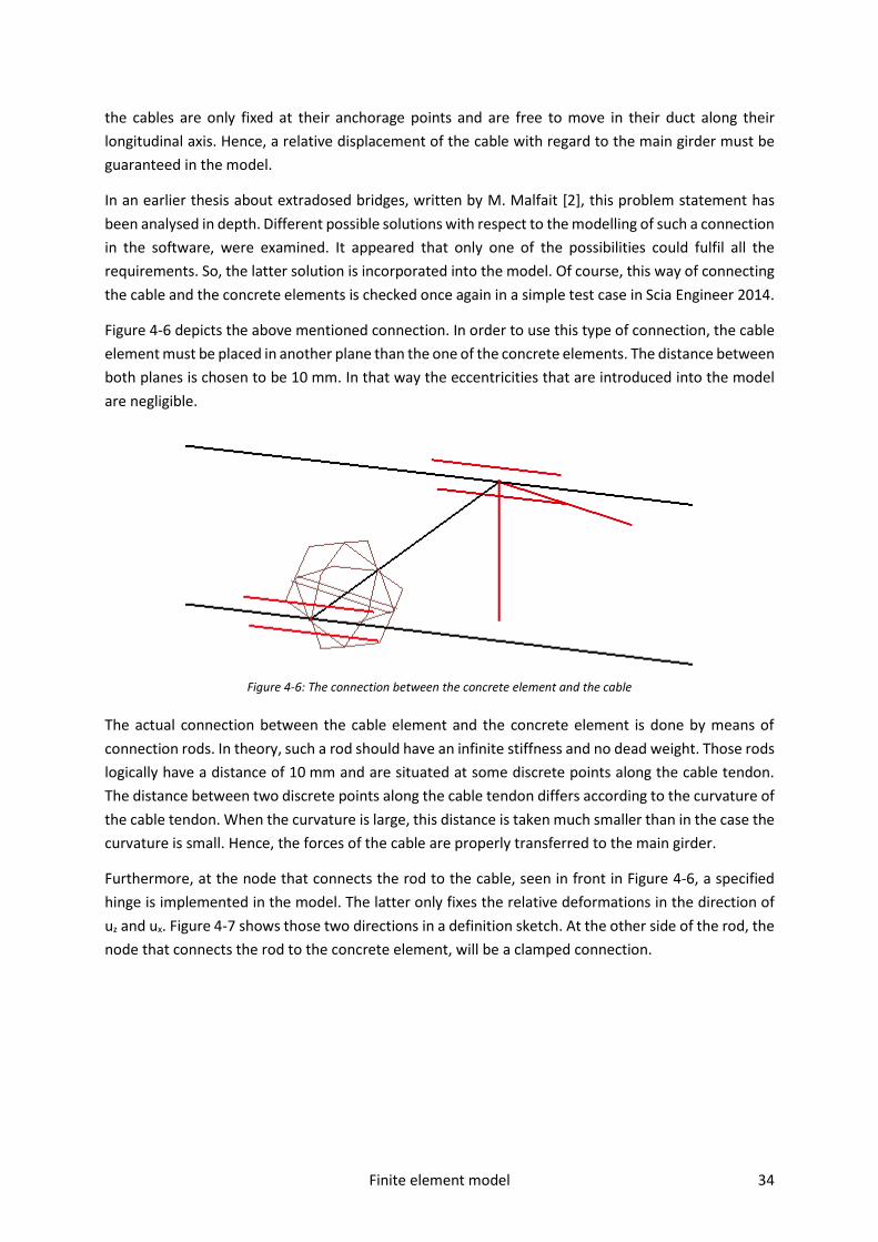
Finite element model 34
the cables are only fixed at their anchorage points and are free to move in their duct along their
longitudinal axis. Hence, a relative displacement of the cable with regard to the main girder must be
guaranteed in the model.
In an earlier thesis about extradosed bridges, written by M. Malfait [2], this problem statement has
been analysed in depth. Different possible solutions with respect to the modelling of such a connection
in the software, were examined. It appeared that only one of the possibilities could fulfil all the
requirements. So, the latter solution is incorporated into the model. Of course, this way of connecting
the cable and the concrete elements is checked once again in a simple test case in Scia Engineer 2014.
Figure 4-6 depicts the above mentioned connection. In order to use this type of connection, the cable
element must be placed in another plane than the one of the concrete elements. The distance between
both planes is chosen to be 10 mm. In that way the eccentricities that are introduced into the model
are negligible.
Figure 4-6: The connection between the concrete element and the cable
The actual connection between the cable element and the concrete element is done by means of
connection rods. In theory, such a rod should have an infinite stiffness and no dead weight. Those rods
logically have a distance of 10 mm and are situated at some discrete points along the cable tendon.
The distance between two discrete points along the cable tendon differs according to the curvature of
the cable tendon. When the curvature is large, this distance is taken much smaller than in the case the
curvature is small. Hence, the forces of the cable are properly transferred to the main girder.
Furthermore, at the node that connects the rod to the cable, seen in front in Figure 4-6, a specified
hinge is implemented in the model. The latter only fixes the relative deformations in the direction of
uz and ux. Figure 4-7 shows those two directions in a definition sketch. At the other side of the rod, the
node that connects the rod to the concrete element, will be a clamped connection.

Finite element model 35
Figure 4-7: Definition sketch of a hinged connection between two rods in Scia Engineer 2014
So, the cable will follow all vertical displacements of the main girder, but it will be able to move freely
in its duct along its longitudinal axis. Last but not least, it must be noticed that the element at the
connection of the stiff rod to the concrete element, seen in the background in Figure 4-6, has only an
auxiliary function in the finite element model. Its function will become clear later on in this chapter.
4.1.4 Overview of the materials used in the model in Scia Engineer 2014
Table 4-1 gives an overview of the different properties of the materials that are used for the elements,
implemented in the model. The properties with respect to the cable tendon are copied from the
material “y1860s7-15.3”, which is already present in the material library of the program. The
characteristics of this material correspond approximately to the ones of the strands given in Annex A
Table 4-1: Overview of the materials used in the model in Scia Engineer 2014
Element type Material name Material type E [MPa] Density [kg/m³]
Cable tendon Cable Strand 1.95 105 7850
Connection rod Infinity Steel 1.0 1010 1
Concrete element C50/60 Concrete 3.73 104 2500
Auxiliary cable Zero Steel 1.0 10-3 1
The values of the modulus of elasticity regarding the materials “Infinity” and “Zero”, are chosen with
respect to some recommendations of the helpdesk of Scia Engineer 2014. According to those people
the stiffness of “Infinity” may not be taken extremely large in order to avoid problems to calculate the
model. A value that is 1000 times larger than the surrounding elements should already be enough to
obtain its purpose to be an infinitely stiff element. An analogue way of thinking can be postulated for
the materials that must have an extremely small stiffness, such as the material “Zero”. Hereby, a value
that is 1000 times smaller should be enough.
Last of all, the helpdesk of Scia Engineer 2014 also recommends not to model materials with a value
of zero with respect to their density, in order to avoid numerical problems. In case such materials may
not have a dead weight in the model, it is suggested to take for example a value of 1 kg/m³.
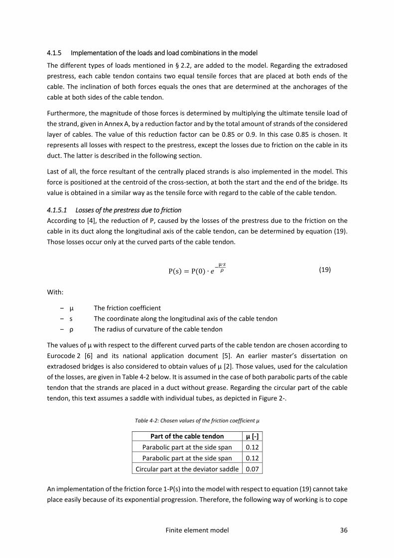
Finite element model 36
4.1.5 Implementation of the loads and load combinations in the model
The different types of loads mentioned in § 2.2, are added to the model. Regarding the extradosed
prestress, each cable tendon contains two equal tensile forces that are placed at both ends of the
cable. The inclination of both forces equals the ones that are determined at the anchorages of the
cable at both sides of the cable tendon.
Furthermore, the magnitude of those forces is determined by multiplying the ultimate tensile load of
the strand, given in Annex A, by a reduction factor and by the total amount of strands of the considered
layer of cables. The value of this reduction factor can be 0.85 or 0.9. In this case 0.85 is chosen. It
represents all losses with respect to the prestress, except the losses due to friction on the cable in its
duct. The latter is described in the following section.
Last of all, the force resultant of the centrally placed strands is also implemented in the model. This
force is positioned at the centroid of the cross-section, at both the start and the end of the bridge. Its
value is obtained in a similar way as the tensile force with regard to the cable of the cable tendon.
4.1.5.1 Losses of the prestress due to friction
According to [4], the reduction of P, caused by the losses of the prestress due to the friction on the
cable in its duct along the longitudinal axis of the cable tendon, can be determined by equation (19).
Those losses occur only at the curved parts of the cable tendon.
P(s) = P(0) ∙ 𝑒−
µ∙𝑠𝜌 (19)
With:
‒ µ The friction coefficient
‒ s The coordinate along the longitudinal axis of the cable tendon
‒ ρ The radius of curvature of the cable tendon
The values of µ with respect to the different curved parts of the cable tendon are chosen according to
Eurocode 2 [6] and its national application document [5]. An earlier master’s dissertation on
extradosed bridges is also considered to obtain values of µ [2]. Those values, used for the calculation
of the losses, are given in Table 4-2 below. It is assumed in the case of both parabolic parts of the cable
tendon that the strands are placed in a duct without grease. Regarding the circular part of the cable
tendon, this text assumes a saddle with individual tubes, as depicted in Figure 2-.
Table 4-2: Chosen values of the friction coefficient µ
Part of the cable tendon µ [-]
Parabolic part at the side span 0.12
Parabolic part at the side span 0.12
Circular part at the deviator saddle 0.07
An implementation of the friction force 1-P(s) into the model with respect to equation (19) cannot take
place easily because of its exponential progression. Therefore, the following way of working is to cope

Finite element model 37
with this aspect of the losses of the prestress. According to M. Malfait [2], first the centroid yP of the
total friction force on the cable must be calculated by means of equations (20), (21) and (22).
A = ∫ 𝑃(𝑥) ∙ 𝑑𝑥 = −𝑃(0)𝑠1
0
𝜌 ∙ (−1 + 𝑒−
µ∙𝑠1𝜌 )
µ (20)
S = ∫ 𝑥 ∙ 𝑃(𝑥) ∙ 𝑑𝑥 = −𝑃(0)𝑠1
0
𝜌 ∙ (−𝜌 + 𝜌 ∙ 𝑒−
µ∙𝑠1𝜌 + µ ∙ 𝑠1 ∙ 𝑒
−µ∙𝑠1
𝜌 )
µ2 (21)
𝑦𝑃 =𝑆
𝐴 (22)
Hereby, the coordinate s in formula (19) is replaced by its projection x on the global x-axis. This
simplification yields, because the curvatures of al curved parts of the cable tendon are rather small.
The coordinate s1 corresponds to the projection of the end-coordinate of a specific curved part of the
cable tendon on the x-axis.
In the case of the cable tendon with respect to the optimal solution B1-5000-1, calculated in the
previous chapter, the values of yP are determined regarding the different curved parts of this cable
tendon. Here, only the parabola at the side span, the circular part of the cable tendon at the tower and
half of the parabola of the mid span are considered. The latter yields, because the relative
displacements of the cable with respect to the main girder change in sign at the axis of symmetry of
the bridge. This is found by a calculation in Scia Engineer 2014.
When those results of yP are divided by the value of s1, used for their calculation respectively, all the
obtained ratios equal more or less 0.5. This means the exponential decrease of the force P can be
approached by a linear decline.
In conclusion, the losses due to friction will be estimated by implementing a constant linear distributed
load along the longitudinal axis of the curved parts of the cable tendon. The direction of these loads is
opposite in sign with respect to the direction of the relative displacements of the cable with regard to
its duct. Its magnitude is equal to the total friction force resultant divided by the respective value of s1.
4.1.5.2 Implementation of the railway traffic
In order to implement LM71 in the model, a module in Scia Engineer 2014, called “traffic loads”, is
used. By means of adding two carriageways to the model, one can create automatically multiple load
cases regarding the different possible positions in which LM71 can be placed on the structure. The
distance between those positions is chosen freely according to the needed accuracy of the model.
Furthermore, all loads with respect to the railway traffic are placed into the proper load groups. Each
load group can be tuned by means of several options. Those options will make sure that for example
no two LM71 are positioned on one track at the same time.

Finite element model 38
4.1.6 Boundary conditions of the model
The boundary conditions are chosen in a way they correspond to the ones stated in § 3.3.2. Figure 4-8
shows the different supports that are used to fulfil the assumed conditions. It has to be noticed that
at the beginning and at the end of the bridge, there are supports underneath the main girder and
underneath the centres of the two tracks as well. When the supports underneath the main girder are
dropped from the model, the main girder will sag between the two supports. The latter will cause some
strange internal forces in the bridge deck that are not desirable. At the intermediate piers there is only
a bearing underneath the main girder. Hence, this creates the possibility to make use of slender piers
at those locations.
Figure 4-8: View of the supports of the model in Scia Engineer 2014
Next, all bearings are chosen to be concentrated in a specified node of the finite element model. This
corresponds to the behaviour of the bearings in reality. Otherwise, in case of the use of line supports,
clamping moments will be taken by the supports. The latter is not feasible in reality, because actual
bearings cannot take those moments.
Furthermore, at the four locations of the supports, longitudinally seen with regard to the boundary
conditions, one of the supports is always fixed in the Y-direction. This is done to overcome problems
in terms of singularities in the matrixes while calculating the results of the model.
Table 4-3 gives an overview of the different settings with respect to all bearings. Herein, the X-direction
corresponds to the longitudinal axis of the bridge, the Y-direction to the transversal axis in the
horizontal plane and the Z-direction to the axis perpendicular to the horizontal plane. Last but not
least, φi summarises all possible rotations around the X-, Y- and Z-axis.

Finite element model 39
Table 4-3: Settings of the different bearings of the model in Scia Engineer 2014
Longitudinal position
Transversal position
Bearing number
X-direction
Y-direction
Z-direction
φi
Start of the
bridge
Track 1 1 Fixed Fixed Fixed
Free
Main girder 2 Free Free Fixed
Track 2 3 Fixed Free Fixed
Pier 1 Main girder 4 Free Fixed Fixed
Pier 2 Main girder 5 Free Fixed Fixed
End of the bridge
Track 1 6 Free Fixed Fixed
Main girder 7 Free Free Fixed
Track 2 8 Free Free Fixed
4.1.7 Mesh of the whole finite element model of the bridge
By means of a rule of thumb the size of the mesh is assumed to be one or two times the thickness of
the 2D-elements. Therefore, a value of 1 m has been chosen.
4.2 USE OF THE MODEL OF THE BRIDGE MADE IN SCIA ENGINEER 2014
In the text below, an explanation is given how to deal with the model and its coupled spreadsheet. The
described methodology is applied in order to obtain all results in the following chapters. Further, a
progressive schema is given in Annex F that has been applied to adjust properly the finite element
model.
4.2.1 Determination of the coordinates of the nodes
First of all, all calculations with respect to the determination of the coordinates of the cable tendon,
the shape of the towers, … have been made by means of a spreadsheet in Excel. The latter is found in
the digital appendix, as listed in Annex K. Here, a spreadsheet for the reference model, i.e. with span
lengths corresponding to the ones from the case study of the bridge in Anderlecht, is given for both a
model with only one cable tendon and a finite element model with two cable tendons.
Once this determination process of the coordinates has been finished, the results are summarised in
a list. The latter can be implemented easily in an interface of Scia Engineer 2014 to adjust all
coordinates at once. In that way, the model in Scia Engineer 2014 is to the spreadsheet of Excel. All
this makes it possible to adjust quickly the geometry of the model.
As mentioned before in § 4.1.3, an auxiliary cable has been added to the model. This is the case for
each cable tendon. The auxiliary cable is applied to adjust easily the coordinates of the cable tendon.
Otherwise, the geometry of the cable cannot be changed at once. By means of this auxiliary cable all
nodes that represent the connection between the concrete main girder and the connection rods, are
replaced in the same way as the ones that connect the rods with the actual cable. Hence, after an
adjustment has been established, each node of the rod keeps the same x- and y-coordinate and its
length remains similar.

Finite element model 40
Of course, the stiffness of the auxiliary cable must be infinitely small and the dead weight has to be
negligible. Both conditions are needed in order that this element should not influence the final results
of the model at all. Its material properties are shown in Table 4-1.
4.2.2 Determination of the loads
The calculation of the friction forces with respect to the prestress as well as the determination of the
tensile forces at both sides of each cable tendon are obtained once again by means of the
spreadsheets, listed in Annex K and given in the digital appendix.
In order to limit the total calculation time, only the most important load cases of LM71 are restrained.
The selection procedure of those significant load cases is done by means of the combination key in
Scia Engineer 2014. Therefore, a so-called “integration-strip” is applied on the 2D-elements that
represent the main girder, in order to transform a 2D-element into a 1D-element. The latter needs to
be achieved to be able to get the combination key of a certain stress resultant in Scia Engineer 2014.
Only some specified stress resultants of the main girder are taken into account to select load cases of
LM71, because in the main girder the most significant normal stresses are located. At the mid - and
side span the maximal value of the bending moment and the maximal value of the torque are
considered. Furthermore, the maximal bending moments at the intermediate piers have also been
taken into account. All the combinations keys with respect to those stress resultants will result in the
most important positions of LM71.
Once each position of the centre of LM71 has been obtained, the coordinates of its point loads can be
determined in Excel. After that, those coordinates can be implemented in Scia Engineer 2014 in a
similar way as described in § 4.2.1, regarding the geometrical properties of the structure.
Furthermore, another simplification has been made with respect to the continuous distributed loads
that make part of LM71. Those loads are always placed on the whole mid - or side span, when those
spans must be loaded. Last of all, the most important results of the model with the reduced load cases
are compared with the ones of the model in which all load cases are implemented. Both models give
rise to the same results, as expected.
All these assumptions and simplifications result in a total number of 22 load cases. Hence, the total
amount of load cases regarding LM71 is reduced a lot, as well as the total calculation time of the finite
element model. It has to be noticed that this methodology is only applied in case there is a change in
the different span lengths of the bridge.

Parametric study of the reference case 41
PARAMETRIC STUDY OF THE REFERENCE CASE
This chapter deals with a parametric study with regard to an optimal saddle - and main girder’s height
of the new concept of extradosed railway bridges with the main girder in a central position. For this
purpose, the model described in the previous chapter has been used to examine the problem
statement.
The parametric study of this chapter is based on the span lengths regarding the case study of the bridge
in Anderlecht. Therefore, this part of the research will be called the parametric study of the reference
case. Furthermore, some of the preliminary conclusions, stated in § 3.4, have been kept in mind in
order to start this parametric study.
5.1 ASSUMPTIONS REGARDING THE PARAMETRIC STUDY OF THE REFERENCE CASE
First of all, one has decided which of the parameters of the model will be kept fixed with respect to
the study. So, the influence of those parameters in order to obtain an optimal solution will not be
verified. From now on, an optimal result corresponds to a solution for which the total amount of
strands needed to counteract the other loads, will be minimal. The parameters that will be researched
in depth are h, h1 and h2.
All other parameters with respect to the cable tendon or the ones corresponding to the bridge deck,
are kept constant or have been linked to the height of the main girder h directly or indirectly. The
geometrical properties of the bridge deck are the same as the ones used in § 3.3, regarding the search
of a cross-section with one centrally placed stiffening girder.
In order to obtain the other relationships or constants with respect to the fixed parameters, some
calculations are executed by means of the model in Scia Engineer 2014. Hereby, the main girder in the
model is chosen to be 3000 mm. H1 has a value of 980 mm.
Figure 5-1: Example of a view of the maximal tensile stresses in the longitudinal direction of the bridge
When all other remaining parameters are set according to the recommendations stated in § 3.2.2, one
obtains the maximal tensile stresses that are shown in Figure 5-1. Those stresses are calculated in the

Parametric study of the reference case 42
longitudinal direction of the bridge and are determined in SLS. In this case, no centrally placed strands
have been introduced into the model.
The total number of strands that is needed to fulfil the requirements described in § 3.2.4, consists of
the sum of two parts of the strands. The first part is represented by the strands of the cable tendon.
The second one refers to the strands that are placed centrally to get rid of the remaining tensile
stresses.
In order to determine this second part of the total amount of strands, it has been decided to restrain
the maximal tensile stress in the neighbourhood of two critical regions of the main girder. The first
region corresponds to the centre of the mid span. The other one is situated at the location where the
position of LM71 corresponds to the maximal bending moment of the side span.
Furthermore, the peak normal stresses at the corners of two or more 2D-elements are neglected. For
the moment, the stresses in the bridge deck, especially the ones at the beginning and at the end of the
bridge, are also ignored. Later on, this part of the stresses will be analysed in depth, i.e. when the
effects of adjusting the positions of the supports are examined.
Figure 5-2: View of the maximal tensile stresses with respect to the optimised solution, without centrally placed strands
In order to determine the relationships or constants with respect to the fixed parameters, each of
those parameters is varied separately, until an optimal solution regarding the total number of strands,
is found. In fact, one searches for a cable tendon that results in an equal magnitude of the maximal
tensile stress in both selected regions. The latter is depicted in Figure 5-2.
In case the centrally placed strands are also added to the model, the solution of the maximal tensile
stresses is the one that can be viewed in Figure 5-3. Here, almost no tensile stresses are still noticeable,
except for some peak stresses at the corners of some 2D-elements.

Parametric study of the reference case 43
Figure 5-3: View of the maximal tensile stresses with respect to the optimised solution, centrally placed strands included
Finally, the following relationships are restrained after having applied above standing methodology.
The parameter a will be kept the same as prescribed in the recommendations of § 3.2.2. Further, the
value of h2 will be set equal to the one of h1. Since the mid span has the largest length of all spans, the
value of u2 is obtained by determining the maximally possible geometrical eccentricity with respect to
the concrete cover. The value of u1 will coincide with the position of the centroid of the cross-section.
5.2 SEARCH FOR AN OPTIMAL VALUE OF H1
Taking into account all assumptions stated in the previous section, one has started to examine the
importance of the saddle height towards the total number of strands. Hereby, the main girder’s height
is kept constant. Its value is chosen to be 3000 mm.
In order to find the optimal value of h1, an iterative process has been used. At the same time it is a
process of trial and error as well. For each value of h1, some calculations are done with regard to
different well guessed amounts of strands of the cable tendon. Of course, each calculation is executed
by means of the model in Scia Engineer 2014 and its coupled spreadsheets in Excel.
Every solution of the model gives rise to a different maximal tensile stress in SLS. This normal stress is
found in the regions described in § 5.1 and is used to determine the additionally needed centrally
placed strands. Therefore, when a set of calculations with respect to a certain h1-value is finished, the
solution with the most minimal value of the total amount of strands is known. The latter corresponds
with a specifically estimated number of strands of the cable tendon. It has to be noticed that the
optimal solution will correspond most of the time with a more or less equal maximal normal stress in
both restrained regions of the main girder.
Then, the above stated method, used to obtain the minimal amount of strands with respect to a certain
h1-value, is repeated until an optimal solution with respect to h1 is clearly found. The latter will be the
solution that gives rise to the smallest total number of strands of all the results.
Table 5-1 contains the results of all optimal solutions regarding each chosen value of h1. Herein, strands
A represents the amount of strands from the cable tendon, strands B represents the ones that are
needed to overcome the remaining tensile stresses. The percentage of each part of the strands in
comparison with the total number of strands is given as well.

Parametric study of the reference case 44
Table 5-1: Overview results regarding the search for an optimal valua of h1 in case h equals 3000 mm
H1 [mm]
side span [MPA]
mid span [MPA]
Strands A
Strands B
Strands Total
Strands A/Total [%]
Strands B/Total [%]
1000 4.6 5.6 57 137 194 29.38 70.62
1500 4.4 5.4 57 133 190 30 70
2000 4.2 4.8 57 118 175 32.57 67.43
2500 4.6 5.3 45 130 175 25.71 74.29
3000 4.4 4.8 45 118 163 27.61 72.39
3500 4.8 4.5 36 118 154 23.38 76.62
4000 4.7 4.2 36 115 151 23.84 76.16
4500 4.7 4.5 36 115 151 23.84 76.16
5000 5.1 5.6 27 137 164 16.46 83.54
Figure 5-4: Overview of all calculations regarding the search for an optimal value of h1 in case h equals 3000 mm
Figure 5-4 shows the resulting total number of strands of all those calculations with respect to the
different saddle heights. Hereby, for example H2000 means a saddle height of 2000 mm. One can see
100
150
200
250
300
350
400
450
500
0 1 0 2 0 3 0 4 0 5 0 6 0 7 0 8 0
TOTA
L N
UM
BER
O
F ST
RA
ND
S [-
]
STRANDS OF THE CABLE TENDON [-]
H1000 H1500 H2000 H2500 H3000
H3500 H4000 H4500 H5000

Parametric study of the reference case 45
that for each saddle height the total amount of strands reaches a minimum according to a specific
amount of strands of the cable tendon. Furthermore, the solution of the optimal value of h1 can also
be viewed, in case the height of the main girder equals 3000 mm. The optimal height of the saddle has
a value somewhere between 4000 mm and 4500 mm.
Next, all minima of the total amount of strands regarding the different saddle heights, i.e. the optimal
solutions with respect to each saddle height, are summarised together in Figure 5-5. When a
regression-analysis is applied upon those results, a relationship between the saddle height and the
total number of strands can be found easily. Apparently, a third order polynomial matches to those
results quite well. This line shows once again that the optimal saddle height is situated in the
neighbourhood of 4000 mm.
Figure 5-5: Overview results regarding the search for an optimal value of h1 in case h equals 3000 mm
Last but not least, also the weights of each part of the strands, namely strands A and strands B, with
respect to the total number of strands, are given in Figure 5-5. After a regression-analysis has been
executed, a relationship between the results can be noticed. Both regression-lines are polynomials of
the second order.
0
10
20
30
40
50
60
70
80
90
100
150
155
160
165
170
175
180
185
190
195
200
0 1 0 0 0 2 0 0 0 3 0 0 0 4 0 0 0 5 0 0 0 6 0 0 0
PA
RT
OF
THE
TOTA
L N
UM
BER
OF
STR
AN
DS
[%]
AM
OU
NT
OF
STR
AN
DS
[-]
H1=H2 [MM]
H = 3 m Strands A, 3 m Strands B, 3 m

Parametric study of the reference case 46
One can see that strands B corresponds to 70 to 85 % of the total amount of strands. Logically, strands
A represents 15 to 30 % of the total number of strands.
5.3 SEARCH FOR AN OPTIMAL VALUE OF H
In order to obtain an optimal value of the height h of the main girder, the process of searching an
optimal value of the saddle height, described in § 5.2, is repeated with respect to different chosen
values of h. Those values of h are selected in such a way that a solution with a minimally needed total
number of strands can be found.
All calculated values regarding the different chosen values of the main girder’s height h are given in a
spreadsheet, which can be found in the digital appendix. This is listed in Annex K. Below, some of the
results and relationships between parameters have been highlighted.
Figure 5-6: Overview results regarding the search for an optimal value of h1 in case of different values of h
Figure 5-6 depicts all optimal values of h1 with respect to the different chosen values of the main
girder’s height h. In fact, all points of one set of solutions on this figure correspond to the minima of
the total amount of strands regarding the different saddle heights. Such a set of points is already given
0
100
200
300
400
500
600
700
800
900
1000
1100
0 2 5 0 0 5 0 0 0 7 5 0 0 1 0 0 0 0 1 2 5 0 0
TOTA
L N
UM
BER
OF
STR
AN
DS
[-]
H1=H2 [MM]
H = 1 m H = 1,5 m H = 2 m H = 3 m H = 4 m H = 5 m H = 6 m

Parametric study of the reference case 47
in Figure 5-5 of the previous section. It can be noticed that a real optimum of the main girder’s height
h regarding an actual minimum of the total number of strands, cannot be found.
A regression-analysis, which is applied on these data, shows that there is a correlation for each set of
the solutions. All regression-lines are polynomials of the third order. The higher the height of the main
girder, the more flat those lines become. In those cases there is a larger uncertainty on the optimal
value of h1.
Figure 5-7: Overview results regarding the search for an optimal value of h in case of different values of h1
By means of all those available results, other relations can be revealed as well. First of all, the
relationship between the total amount of strands and the height of the main girder is analysed. The
latter is shown in Figure 5-7. Hereby, the relationship is depicted with respect to different values of h1.
The regression-lines through those data-sets all have a correlation coefficient r of 0.95 or more1. In
those cases one has opted for a regression-analysis with power functions, as given in equation (23).
Herein A and B correspond to two unknown coefficients, which depend on the boundary conditions.
f(x) = A ∙ 𝑥𝐵 (23)
1 Excel will determine the correlation between two parameters by means of the Pearson-correlation coefficient.
0
100
200
300
400
500
600
700
800
900
1000
1100
0 1 0 0 0 2 0 0 0 3 0 0 0 4 0 0 0 5 0 0 0 6 0 0 0
TOTA
L A
MO
UN
T O
F ST
RA
ND
S[-
]
H [MM]
H1 = H2 = 1000 mm H1 = H2 = 2000 mm H1 = H2 = 3000 mm
H1 = H2 = 4000 mm H1 = H2 = 5000 mm H1 = H2 = 6000 mm

Parametric study of the reference case 48
Due to the properties of power functions, the first part of the curves shows a peak towards an
asymptotic value. From a certain transition point on those curves, the relationship can be
approximated by a linear line.
Furthermore, in Figure 5-8 one can see the relationship between the optimal amount of strands with
respect to the different values of the height of the main girder. Keeping in mind the previous results,
it may not be surprising that the related regression-line is a decaying power function. Hence, there will
be no real optimum, i.e. a minimal value of the total amount of strands.
Figure 5-8: The optimal number of strands and its relative part of the strands B regarding the main girder’s height
Figure 5-8 also contains a view of the relation between the additional placed strands B, expressed in a
percentage of the total number of strands, and the height h of the main girder. The regression-analysis
shows a decreasing power function. The values that are linked to that function lay between 70 and
90 %. When for all the solutions that are depicted in Figure 5-7, the relative values of their part B should
be drawn on one graph, one will find a much larger range for those percentages. In that case all values
will be situated from 50 to 95 %. The latter can be seen on a graph in the spreadsheet that is given in
the digital appendix.
20
30
40
50
60
70
80
90
100
0
100
200
300
400
500
600
700
800
0 1 0 0 0 2 0 0 0 3 0 0 0 4 0 0 0 5 0 0 0 6 0 0 0 7 0 0 0P
AR
T ST
RA
ND
S B
REG
AR
DIN
G T
HE
TOTA
L N
UM
BER
OF
STR
AN
DS
[%]
AM
OU
NT
OF
STR
AN
DS
[-]
H [MM]
Optimal amount of strands Percentage of the additional needed strands

Parametric study of the reference case 49
Figure 5-9: The optimal saddle height with respect to the height of the main girder
Last but not least Figure 5-9 shows that a relationship exists between the optimal height of the saddle
h1 and the height of the main girder h. A parabola can be determined as a regression-line.
5.4 CONCLUSIONS WITH RESPECT TO THE REFERENCE CASE
First of all, the parametric study of the reference case reveals two main conclusions with respect to
the two non-fixed parameters. The first one is related to the search for an optimal value of h1. An
optimal value of the saddle height is always found, regarding a certain value of the height of the main
girder. This is shown in Figure 5-6 and in Figure 5-9. The latter figure proves that the higher the height
of the main girder will be, the higher the optimal value of the height of the saddle will become. The
relationship between both parameters is a second order polynomial.
Furthermore, it is noticeable that the larger the height of the main girder becomes, the less easy the
optimal value of the saddle height h1 can be determined. So, the uncertainty on the results of the
optimal saddle height enlarges in the case of an increasing value of h. This can be viewed in Figure 5-6.
The regression-lines are more flattened out in the case of a larger height of the main girder. Therefore,
in those cases the choice of the saddle height will be less important with respect to the total number
of strands.
Looking at the second non-fixed parameter, an optimal value for the height of the main girder cannot
be found. Figure 5-7 and Figure 5-8 depict that the relationship between the total amount of strands
and the main girder’s height h is a decaying power function. Here, one can also notice that an increase
of the moment of inertia, i.e. a larger height of the main girder, will result in a decrease of the total
amount of strands.
0
2000
4000
6000
8000
10000
12000
0 1 0 0 0 2 0 0 0 3 0 0 0 4 0 0 0 5 0 0 0 6 0 0 0 7 0 0 0
OP
TIM
AL
SAD
DLE
HEI
GH
T [M
M]
H [MM]

Parametric study of the reference case 50
However, it is not feasible to increase the main girder’s height h infinitely. Moreover, from a certain
point the benefits in terms of a decrease in the total amount of strands will become less significant.
Those profits even disappear completely from a certain height of the girder. In that case the profits
with regard to the total number of strands are nullified by the increasing area and weight of the cross-
section.
Above mentioned conclusion can be noticed in Figure 5-6, because there the vertical distance between
the curves becomes smaller in the case of an enlarging height of the stiffening girder. It is also visible
in Figure 5-7, where the decay almost becomes zero in the case of large values of h.
Furthermore, there is a visual limit as well, with respect to the main girder’s height. In the next chapter
this will be explained briefly. Besides an upper boarder of the main girder’s height h, there is also a
lower limit worth mentioning. From a certain height of the main girder the regression-lines depicted
in Figure 5-7 and Figure 5-8, can be approximated by linear lines. On those figures this transition point
is situated at a height of the main girder of about 2000 mm.
The range between those two above described limits contains all feasible solutions. Whether the
ultimately chosen solution has more concrete area and less strands or the opposite, depends on the
requirements and the boundary conditions. Pure visually, the solution with the smallest height h will
always be preferred. Nevertheless, the final solution can also depend on the availability and the costs
of the different materials. Then, it is not unlikely that a solution with a larger height of the main girder
is preferred.
So far only the verification of the normal stresses and the resulting needed number of strands has been
discussed. However, the deformations must be checked as well. When the deformations are
determined in the way that is described in § 3.2.5, both the deflections and the rotations are found, as
can be viewed in Figure 5-10 and Figure 5-11. It has to be noticed that those deformations are obtained
by taking into account only one by LM71 loaded track. All other loads, including the prestress, must be
ignored according to the Eurocodes.
Looking at the maximal and minimal deflections that are situated at the side - and mid span of the
bridge, all the solutions with a height of the main girder smaller than 2000 mm do not fulfil the
requirements. Hereby, the maximal deflections correspond to a downward deformation. In contrary,
the minimal deflections are measured in the opposite direction. The requirements regarding the
passengers comfort have already been described in § 3.2.5.

Parametric study of the reference case 51
Figure 5-10: Deflections of the different solutions of the reference case
Figure 5-11: Rotations of the different solutions of the reference case
0
50
100
150
200
250
300
350
0 1 0 0 0 2 0 0 0 3 0 0 0 4 0 0 0 5 0 0 0 6 0 0 0 7 0 0 0
DEF
LEC
TIO
N [
MM
]
H [MM]
Uz,max,span1 Uz,min,span1 Uz,max,span2 Uz,min,span2
0
2
4
6
8
10
12
14
16
18
0 1 0 0 0 2 0 0 0 3 0 0 0 4 0 0 0 5 0 0 0 6 0 0 0 7 0 0 0
RO
TATI
ON
[M
RA
D]
H [MM]
Theta,max,begin Theta,min,begin

Parametric study of the reference case 52
Above all, neither the rotations do fulfil the condition of the maximally allowed inclination angle that
is described in § 3.2.5, when the height h of the stiffening girder reaches values lower than 2000 mm.
Hence, the earlier mentioned transition point, which can be seen in Figure 5-7 and Figure 5-8 and gives
rise to the lower limit of the range for feasible main girder’s heights, coincides with the lower boarder
of height h according to the deformations.
Finally, when observing Figure 5-8, it has to be highlighted that the part of the strands that corresponds
to the centrally placed ones, will be at least 70 % or more. As mentioned before, the higher the height
of the main girder becomes, the smaller this percentage will be. So, the strands of the cable tendon
itself are just a small part of the total amount of strands. Therefore, one can postulate the question if
the extradosed reinforcement is an economical and feasible solution.
In order to study further this new concept, some scale enlargements have to be executed in the next
chapter to analyse the influences on the saddle - and the main girder’s height. Furthermore, by
enlarging the different spans, one can also investigate if the part of the additional placed strands,
relative to the total amount of strands, will change or not.
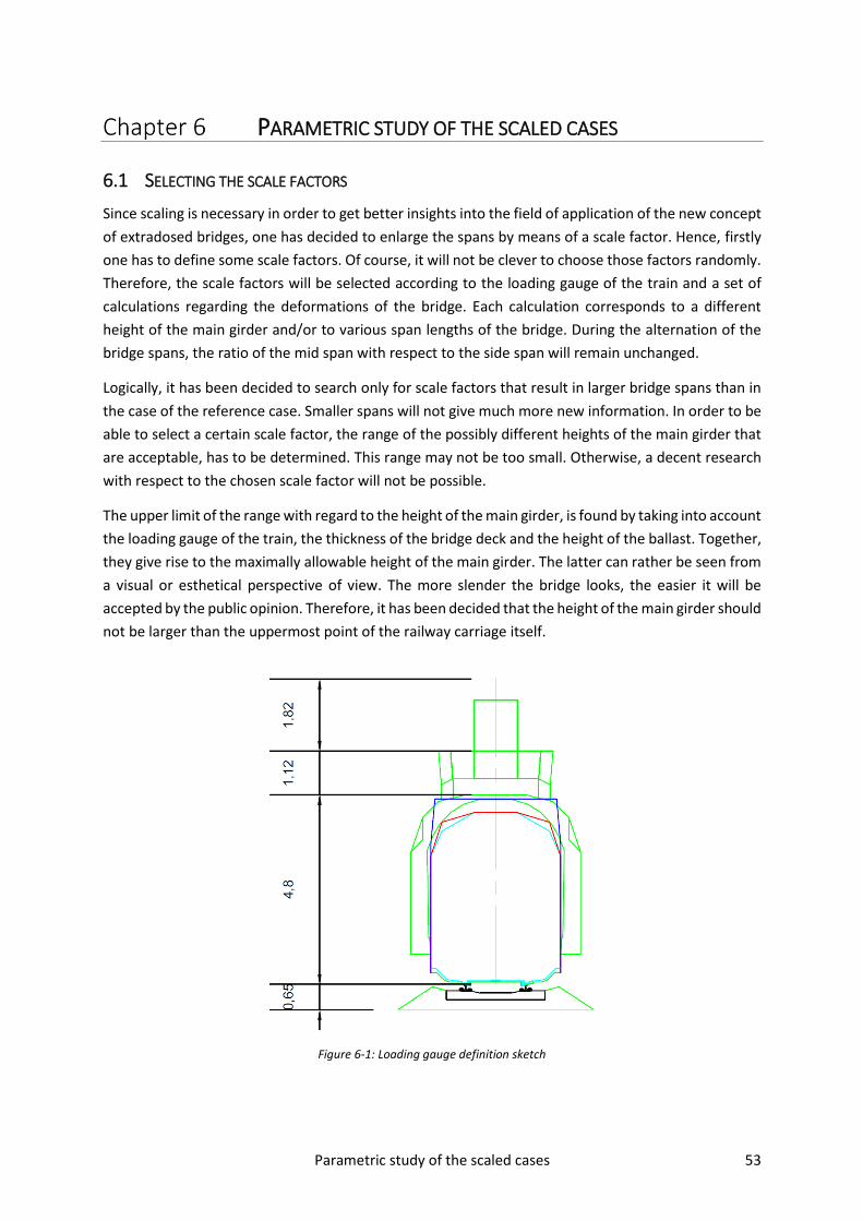
Parametric study of the scaled cases 53
PARAMETRIC STUDY OF THE SCALED CASES
6.1 SELECTING THE SCALE FACTORS
Since scaling is necessary in order to get better insights into the field of application of the new concept
of extradosed bridges, one has decided to enlarge the spans by means of a scale factor. Hence, firstly
one has to define some scale factors. Of course, it will not be clever to choose those factors randomly.
Therefore, the scale factors will be selected according to the loading gauge of the train and a set of
calculations regarding the deformations of the bridge. Each calculation corresponds to a different
height of the main girder and/or to various span lengths of the bridge. During the alternation of the
bridge spans, the ratio of the mid span with respect to the side span will remain unchanged.
Logically, it has been decided to search only for scale factors that result in larger bridge spans than in
the case of the reference case. Smaller spans will not give much more new information. In order to be
able to select a certain scale factor, the range of the possibly different heights of the main girder that
are acceptable, has to be determined. This range may not be too small. Otherwise, a decent research
with respect to the chosen scale factor will not be possible.
The upper limit of the range with regard to the height of the main girder, is found by taking into account
the loading gauge of the train, the thickness of the bridge deck and the height of the ballast. Together,
they give rise to the maximally allowable height of the main girder. The latter can rather be seen from
a visual or esthetical perspective of view. The more slender the bridge looks, the easier it will be
accepted by the public opinion. Therefore, it has been decided that the height of the main girder should
not be larger than the uppermost point of the railway carriage itself.
Figure 6-1: Loading gauge definition sketch

Parametric study of the scaled cases 54
Figure 6-1 shows a sketch of the loading gauge that is used to determine the height of the railway
carriage. The loading gauge, without the catenary and the ballast, has a height of about 4.8 m.
As mentioned before, the thickness of the bridge deck follows from an estimation that is described in
§ 3.3.1. Its value is 0.450 m. The height of the ballast is assumed to be 0.750 m. The latter is an average
value. Hence, when the three parameters are added together, one finds the upper limit of the range
with regard to the height of the main girder, namely 6 m.
Furthermore, the lower limit of this range is obtained by means of the requirements of the allowable
deformations of the bridge. They are described in § 3.2.5. The values of the maximal deflections are
given in Table 6-1 and depend on the different chosen scale factors. By contrast, the value of the
maximal inclination at the transition of the abutment and the bridge deck is independent of the chosen
scale factor. Its value remains 0.0035 rad for all cases.
Table 6-1: Upper limits of the deflections according to different scale factors
Scale factor L1 [m] L2 [m] δspan1 [mm] δspan2 [mm]
1 29 42 26.85 49.12
1.5t 43.5 63 40.28 73.68
2 58 84 53.70 98.25
2.5 72.5 105 67.13 122.81
Figure 6-2: Maximal deflection at side- and mid span with respect to different scale factors
Figure 6-2 shows an overview of the optimal solutions regarding the minimal and maximal deflections
with respect to different scale factors. It has to be noticed that those deflections, both at the side span
and mid span, are calculated by means of all the load cases that are generated by the module “traffic
0
10
20
30
40
50
60
70
80
90
100
0 0 , 5 1 1 , 5 2 2 , 5 3
VER
TIC
AL
DEF
LEC
TIO
N [
MM
]
SCALE FACTOR [-]
Uz,max,span1 Uz,min,span1 Uz,max,span2 Uz,min,span2

Parametric study of the scaled cases 55
loads” in Scia Engineer 2014. So, the simplification with respect to the load cases, which is described
in § 4.2.2, is not applied here because of the preconceived accuracy of the calculations.
In this context “optimal” means that for each chosen scale factor, the minimally allowable value of the
height of the main girder, for which the solutions of the deflections just fulfil the requirements of the
deformations, will be determined. The values of those minimal heights that correspond to the scale
factors in Figure 6-2, are found in Table 6-2 below. Apparently, there is a linear relationship between
the scale factors and the values of hmin. The same relationship can be found between the scale factors
and the different calculated deflections as well.
Table 6-2: Minimal values of the main girder’s height regarding the scale factors
Scale factor hmin [mm]
1 2000
1.5t 3000
2 4000
2.5 5000
In a next step, the maximal and minimal inclination angles at the transition of the abutment and the
bridge deck are verified. They are given in Figure 6-3, with respect to the above chosen scale factors.
One can notice that the relation between the different solutions and the scale factors is linear.
Moreover, in the case of the minimal inclination angle at the transition, all values are almost equal.
Figure 6-3: Maximal rotation at the transition between bridge deck and abutment with respect to different scale factors
0
0,5
1
1,5
2
2,5
3
3,5
4
0 0 , 5 1 1 , 5 2 2 , 5 3
RO
TATI
ON
[M
RA
D]
SCALE FACTOR [-]
Theta,max,begin Theta,min,begin

Parametric study of the scaled cases 56
In Figure 6-3 it can also be seen that the maximal inclination angle regarding a scale factor of 2.5 is
larger than 0.0035 rad. Hence, the latter scale factor will not be selected. A larger value of the minimal
height of the main girder may fulfil all conditions of the deformations. Nevertheless, in that case the
upper and lower limit of the range will almost coincide. Therefore, when the scale factor is 2.5, the
range will be too small to obtain proper results.
Finally, the following values of the scale factors are restrained: 1.5, 1.75 and 2. By means of those scale
factors a comparison with respect to the reference case can be made properly. All selected factors
correspond to a feasible range with regard to the height of the main girder. The scale factor 1.75 is not
verified in depth, but one has assumed that the deformations and the value of the lower limit of h can
be found easily by a linear interpolation of the above shown curves and results.
Once more, all results with respect to this paragraph are given in a spreadsheet in Excel, which can be
found in the digital appendix, as listed in Annex K. The used models in Scia Engineer 2014 are stored in
the digital appendix as well.
6.2 RESULTS OF THE SCALED CASES
Before starting the actual calculations with respect to a specified scaled case, the most severe load
cases have to be defined, as stated in § 4.2.2. For each scaled case, the resulting models in
Scia Engineer 2014 are listed in Annex K and given in the digital appendix.
Furthermore, all assumptions that have been made regarding the calculations of the reference case,
are equal to the ones that are used with respect to every parametric study of a scaled case. Hence, the
whole methodology that is applied here in this chapter, in order to find optimal values of the saddle
height h1 and the height of the main girder h, is almost identical to the one that is described in the
previous chapter. In fact, the same exercise as for the reference case has been done over again for the
different scale factors.
Next, some of the solutions of all those calculations with respect to the different scaled cases are given
in Annex G. Only the most important results are shown in this annex. The other ones can be consulted
in the digital appendix. Obviously, for every set of solutions regarding a certain scale factor, quite
analogue conclusions can be found as described in § 5.4.
Furthermore, the relationships, which follow from the regression-analyses between the different
parameters, are also very similar to the ones, which are found in the previous chapter. It has to be
noticed that all power functions can be more or less approximated by linear functions. Due to the fact
that the possible heights of the main girder have already been limited beforehand by a certain range
regarding the requirements of the deformations and the loading gauge of the train, all power functions
start after their transition point.
6.2.1 Comparison between the results of the scaled cases and the reference case
As all the solutions with respect to the different scaled cases have been known now, one can make an
analysis of the relationships between the results of the different scale factors and the reference case.
In order to be able to make the analysis between the parameters properly, only the most significant
solutions of each scaled case and the reference case as well are selected. Hence, it has been decided

Parametric study of the scaled cases 57
to restrain just all solutions that correspond to the optimal total amount of strands with respect to a
specified height of the main girder.
Those results are summarised in Table 6-3 below. Herein strands A represents the number of strands
with respect to the cable tendon and strands B corresponds to the strands that are placed centrally to
counteract the remaining tensile normal stresses. In the last two columns of the table, their part,
relative to the total number of strands, is calculated as a percentage.
Table 6-3: Overview optimal results of the reference case and all scaled cases
Scale factor
H
[mm] H1
[mm] side span [MPA]
mid span [MPA]
Strands A
Strands B
Strands Total
Strands A/Total
[%]
Strands B/Total
[%]
1 1000 2000 39.3 40.2 74 696 770 9.61 90.39
1 1500 2500 16.9 17.1 57 327 384 14.84 85.16
1 2000 3500 10.4 10.4 39 218 257 15.18 84.82
1 3000
4000 4.7 4.2 36 115 151 23.84 76.16
1.5 5500 9.9 9.2 66 243 309 21.36 78.64
1
4000
5500 3 3.2 30 90 120 25 75
1.5 6500 6.3 6.2 57 177 234 24.36 75.64
1.75 6500 8.4 8.4 74 236 310 23.87 76.13
2 6500 10.7 10.7 96 301 397 24.18 75.82
1
5000
7500 2.1 2.1 29 67 96 30.21 69.79
1.5 8000 4.6 4.5 50 146 196 25.51 74.49
1.75 8000 6.1 6.1 65 194 259 25.10 74.90
2 7500 7.6 7.1 93 241 334 27.84 72.16
1
6000
11000 1.8 1.8 22 64 86 25.58 74.42
1.5 8500 3.4 3.4 50 120 170 28.74 71.26
1.75 8500 4.6 4.6 65 163 228 28.51 71.49
2 9000 6 5.9 81 212 293 27.65 72.35
Figure 6-4 shows the total number of strands of all sorted out solutions with respect to the height of
the main girder. Those solutions are grouped according to the different lengths of the mid span. The
latter correspond to the specified values of the scale factors. So, for example the reference case will
be represented by a mid span length of 42 m and a scale factor 2 by a value of L2 of 84 m. Furthermore,
a regression-analysis shows that power functions match the best for the relationships between all
grouped solutions.

Parametric study of the scaled cases 58
Figure 6-4: Optimal total number of strands with respect to the height of the main girder
Figure 6-5: Optimal height of the saddle with respect to the height of the main girder
Next, the height of the saddle is analysed with respect to the height of the main girder. This is depicted
in Figure 6-5. Here, the solutions are also grouped together according to the different mid span lengths
0
100
200
300
400
500
600
700
800
900
0 1000 2000 3000 4000 5000 6000 7000
TOTA
L N
UM
BER
OF
STR
AN
DS
[-]
H [MM]
L2 = 42 m L2 = 63 m L2 = 73,5 m L2 = 84 m
0
2000
4000
6000
8000
10000
12000
0 1000 2000 3000 4000 5000 6000 7000
OP
TIM
AL
SAD
DLE
HEI
GH
T [M
M]
H [MM]
L2 = 42 m L2 = 63 m L2 = 73,5 m L2 = 84 m

Parametric study of the scaled cases 59
that correspond to the chosen scale factors. In this case a linear relationship can be determined
between those parameters, when a regression-analysis is applied.
Furthermore, for each different acceptable height of the main girder, the total number of strands is
compared with respect to the different lengths of the mid span. The latter is shown in Figure 6-6.
Hereby, all combined groups of results exhibit clearly a linear relation with regard to the different
values of L2.
Figure 6-6: Optimal total number of strands with respect to the length of the mid span
In a similar way, one has searched for a relationship between the different solutions of the heights of
the saddle and the length of the mid span. In this case, the different solutions of the heights of the
saddle are analysed together with respect to the different values of the main girder’s heights, which
can be seen in Figure 6-7.
In case a value of h of 4 m or 6 m is picked out, the relationship between the parameters in this figure
is given by a second order polynomial. However, both parabolas have a different sign regarding their
value of the curvature. By contrast, when a value of h equal to 5 m is selected, the best fitting function
will be a linear line. Hence, for all cases no specified relationship can be determined.
0
50
100
150
200
250
300
350
400
450
35 40 45 50 55 60 65 70 75 80 85 90
TOTA
L N
UM
BER
OF
STR
AN
DS
[-]
L2 [M]
H = 4 m H = 5 m H = 6 m

Parametric study of the scaled cases 60
Figure 6-7: Optimal height of the saddle with respect to the length of the mid span
After that, the values of the relative parts of the strands B with respect to the total number of the
strands respectively are examined regarding the different values of L2. The latter is shown in Figure
6-8. As for the analysis before, the results are grouped together according to the different allowable
heights of the main girder.
When one searches for a relationship between those parameters, again no balanced solution is found
by a regression-analysis. In case the value of h is 4 m, the relation between both parameters will be
linear. However, when h equals 5 or 6 m, two parabolas that differ in sign with respect to the curvature,
are found.
5000
6000
7000
8000
9000
10000
11000
35 40 45 50 55 60 65 70 75 80 85 90
OP
TIM
AL
DEV
IATO
R S
AD
DLE
HEI
GH
T [M
M]
L2 [M]
H = 4 m H = 5 m H = 6 m

Parametric study of the scaled cases 61
Figure 6-8: Relative part of the strands B towards the total number of strands with respect to the length of the mid span
Figure 6-9: Multiplication factor of the total number of strands of the reference case with respect to different scale factors
60
62
64
66
68
70
72
74
76
78
80
35 40 45 50 55 60 65 70 75 80 85 90
REL
ATI
VE
PA
RT
STR
AN
DS
B R
EGA
RD
ING
TH
E TO
TAL
NU
MB
ER O
F ST
RA
ND
S [%
]
L2 [M]
H = 4 m H = 5 m H = 6 m
0,5
1
1,5
2
2,5
3
3,5
0,9 1 1,1 1,2 1,3 1,4 1,5 1,6 1,7 1,8 1,9 2 2,1
MU
LTIP
LIC
ATI
ON
FA
CTO
R T
OTA
L N
UM
BER
OF
STR
AN
DS
[-]
SCALE FACTOR [-]

Parametric study of the scaled cases 62
Finally, one has searched for a relationship regarding a factor, with which the total amount of strands
with respect to a certain solution of the reference case has to be multiplied in order to obtain an
estimation of the total number of strands that is needed for a specified scaled case.
For this purpose, the values of the total amount of strands of the scaled cases are divided by the total
number of strands of the reference case. Of course, in order to obtain such a ratio, both values of this
ratio must correspond to an equal value of the height of the main girder. Figure 6-9 shows all those
ratios with respect to the different scale factors. Since all points regarding a certain value of the scale
factor coincide more or less, the search for a relationship between a multiplication factor and a scale
factor will be appropriate. When a regression-analysis is executed on the results shown in Figure 6-9,
a linear relationship between those earlier mentioned parameters can be obtained.
It has to be noticed that one can determine a relationship for a multiplication factor in order to obtain
the amount of cables needed with respect to the strands of the cable tendon or to the centrally placed
strands as well. However, there is a larger uncertainty regarding the calculated linear line in the case
of the factor with respect to the strands of the cable tendon than in the case of the factor regarding
the additional needed strands.
As described in Annex K, all spreadsheets that contain the results of the scaled cases separately and
the spreadsheet that contains the global comparison, are found in the digital appendix.
6.3 CONCLUSIONS WITH RESPECT TO THE PARAMETRIC STUDY OF THE SCALED CASES
As mentioned before in § 6.2, the conclusions with respect to the results of the scaled cases are
separately very similar to the ones regarding the reference case. The latter are described in § 5.4.
Hence, only the conclusions with respect to the comparison of the solutions of all the scaled cases and
the reference case, will be highlighted in this part of the text.
First, Figure 6-4 and Figure 6-6 show that, when the span lengths are scaled, namely enlarged, the total
number of strands that is necessary to counteract the internal forces, will increase linearly. The higher
the height of the main girder becomes, the less strong that increase will be. All this this seems quite
logical, because an enlargement of the length of the span will give rise to an increase of the bending
moments, due to the enlargement of the internal lever arm. Consequently, the normal stresses, which
have to be counteracted by the prestress, will become larger as well.
Another conclusion that can be made with respect to Figure 6-4 and Figure 6-6 is that for each scale
factor, a larger height of the main girder results in a decay of the total number of strands. This decay
occurs according to a power function. The decrease is caused by a growth of the moment of inertia of
the cross-section due to the increase of parameter h. As highlighted in the previous chapter, from a
certain point, the profits of needing less strands, which occurs by enlarging the height of the main
girder, will disappear almost completely or be nullified by the disadvantage of needing more concrete
regarding the area of the cross-section.
Next, in Figure 6-5 and in Figure 6-7 one can see that regardless the scale factor, an increase of the
height of the main girder will result in a larger optimal value of the height of the saddle. However, no
general relation can be put forward between the height of the saddle and the different values of the
scale factor. The relationship between those parameters depends on the height of the main girder and

Parametric study of the scaled cases 63
can be linear or parabolic. Those parabolas can even differ in sign regarding their value of the
curvature.
In addition to the above given conclusions with respect to the height of the saddle, it has to be noticed
that within a certain range, the choice of the height of the saddle will not influence the totally needed
amount of strands so much. Of course, the statement only yields when the height of the main girder
and the scale factor are fixed to a specified value. Because of all this, the search for an optimal value
of h1 is rather difficult. The latter may be the reason of not finding an explicit relationship between h1
and the scale factors.
Furthermore, after analysing the parts of “strands B” with respect to the total number of the strands
respectively, in the case of different scale factors as shown in Figure 6-8, it appears that scaling the
spans of the bridge will not change the magnitude of the values of this percentage that much. Figure
6-8 and Table 6-3 depict that all calculated values of this ratio are still situated between 70 and 76 %.
Hence, the question that is postulated at the end of § 5.4 still cannot be answered profoundly in a
positive sense after having scaled the dimensions of the bridge. However, regarding all collected
results so far, this new concept seems to be rather an uneconomical choice, because more than 50 %
of the strands is needed to overcome tensile stresses that cannot be counteracted by the prestress of
the extradosed cables.
Again, after a regression-analysis is applied on those results, no clear relationship is found between
those relative parts and the scale factors. The only conclusion that yet can be made, is that the higher
the values of h become, the smaller the relative part of the centrally placed strands will be.
A linear relationship is found between the scale factors and the multiplication factor of the total
number of a specified part of the strands, regarding the solutions of the reference case. As mentioned
before, the advantage of such a multiplication factor is that it can be used to obtain a fast estimation
of the total number of strands or a certain part of the strands that is needed with respect to a scaled
case. Of course, one already has to know the solution of a reference case beforehand in order to be
able to use this multiplication factor.
Finally, it has to be noticed that all clear relationships, which are given in this section and which are
determined with respect to the scale factors, are linear lines. This is also the case for the deformations
of the bridge, as one can see in Figure 6-2 and Figure 6-3. Furthermore, it can be repeated that the
choice of the height of the main girder with respect to a certain value of the scale factor, is free within
a specified range. The latter is determined in § 6.1. As mentioned before in § 5.4, the ultimate choice
will depend on the requirements that are attached to the bridge.

Parametric study of the boundary conditions 64
PARAMETRIC STUDY OF THE BOUNDARY CONDITIONS
So far, the new concept of extradosed railway bridges with the main girder in a central position has
been analysed in depth with respect to the shape of the cable tendon, the normal stresses and
deformations of the main girder itself and the optimal values of h and h1. Hereby, the stresses and
deformations regarding the bridge deck have been ignored. Hence, only a global research on this
concept has been executed so far.
Therefore, in this chapter some local effects as the deck twist and the normal stresses in the bridge
deck, especially at the start and at the end position of the bridge, are studied more in detail.
Meanwhile, the influence of the different values of the spacing of the supports at the beginning and
at the end of the bridge can also be examined.
7.1 VERIFICATION OF THE DECK TWIST
In order to be able to verify the deformations of bridge deck, besides the maximally allowable vertical
deflection of the track with respect to the comfort of the passengers, the deck twist has to be
determined according to the RTV KW01 [17]. In this guideline, which is made by Infrabel, one refers to
the Eurcode 0 [12] and its national application document [16] in order to obtain more detailed
information about the requirements regarding the deck twist.
Figure 7-1: Definition sketch of the deck twist t
In Figure 7-1 a definition sketch of the deck twist t is given. Hereby, the four corners of the rectangle
represent the four wheels of a bogie of the train. In this figure the track gauge s is depicted as well. Its
value is 1.435 m. Since the speed of the train has been chosen to be 160 km/h, the maximally allowed
deck twist has a value of 3 mm/3 m. The deck twist is measured between one of the four wheels and
a plane that goes through the three other remaining wheels.
According to Eurocode 0 this deck twist has to be verified at all the positions where such a bogie can
be situated. Moreover, it has to be calculated in the case of the worst possible load cases due to LM71.
The other loads may not be taken into account.
For this matter, the most governing positions of LM71 are determined by means of influence lines. It
appears that those positions coincide with the ones corresponding to the largest value of the bending
moment at the side span and the maximal torsional moment at the same side span. Both maximal
moments are found after a calculation in Scia Engineer 2014 regarding the internal forces due to the
railway traffic, in case LM71 acts only on track 1.
Next, the vertical deflections have been calculated at some specified chosen points at the start of the
bridge deck. Those points are located underneath both rails of track 1 and have a spacing of 1 m.

Parametric study of the boundary conditions 65
Hence, it is possible to obtain the maximal value of the deck twist for every meter the bogie advances
along track 1. An example of such a calculation of the deflections in Scia Engineer 2014 is given in
Figure 7-2 below.
Figure 7-2: Example of a calculation of the vertical deflections with respect to de determination of the deck twist
Once those deflections have been gathered, the maximal value of the deck twist t can be determined
in a spreadsheet in Excel. For each above mentioned position of the bogie, the calculation of the deck
twist is done by means of equation (24). The latter represents the perpendicular distance between a
point Q (xQ, yQ, zQ) and a plane α. This plane α is given by equation (25). Herein, the constants u, v, w
and r depend on the boundary conditions. When three points of a plane are known, those constants
can be determined by means of a linear system.
d(𝛼, 𝑄) =|𝑢 ∙ x𝑄 + v ∙ y𝑄 + w ∙ z𝑄 + r|
√𝑢2 + 𝑣2 + 𝑤2 (24)
𝛼: 𝑢 ∙ x + v ∙ y + w ∙ z + r = 0 (25)
In fact, by means of above standing equations, one can calculate four different values of the deck twist,
for each position of the bogie. Four different combinations of three deflections of the bogie can be
distinguished, for which a solution of α is found. So, for each selected plane, the distance towards the
respectively remaining deflection can be determined. Eventually, the ultimate value of the deck twist
with respect to a certain position of the bogie, is obtained by picking the maximal value of those four
calculated distances.
Finally, the result of a calculation of the deck twist is shown in Figure 7-3. Herein, the two
developments of the deck twist are depicted with respect to a coordinate x along the longitudinal axis
of track 1. One of the lines corresponds to the load case that results in the maximal bending moment
of the main girder at the side span. The other one corresponds to the load case that gives rise to the

Parametric study of the boundary conditions 66
maximal value of the torque at that span. Both lines represent the deck twist t in case the optimal
solution of the previous chapter has a height of the main girder of 4 m and a scale factor 1.75.
Figure 7-3: Comparison results deck twist t regarding the two restrained load cases
When next both developments are compared to each other, it can be noticed that they do not differ a
lot. The latter conclusion is also found in the case of other preliminary calculations of the deck twist.
Therefore, it has been decided to determine only one of those developments regarding the further
analysis of the deck twist in this chapter. Hence, the load case corresponding to the maximal bending
moment at the side span is chosen to be the load case that will be used to calculate the deck twist.
Consequently, the total calculation- and processing-time will be reduced.
The spreadsheet in Excel and all the models in Scia Engineer 2014 that are used to determine the deck
twist, are given in the digital appendix and are listed in Annex K.
7.2 DEFINING THE PROBLEM STATEMENT
Since this chapter deals with the research of some local effects, it will be neither feasible, nor necessary
to perform a parametric study of the boundary conditions with respect to all the optimal solutions.
The latter are given in Table 6-3. A specified set of solutions will already be satisfactory in order to
obtain proper results and to deduct reliable conclusions. Therefore, the choice has been made to select
only the optimal solutions regarding a specific scale factor. Its value is preferred to be 1.75, because
this data-set is situated somewhere in the middle of the range of the total bunch of solutions.
Table 7-1 shows this selected data-set of solutions once again. The explanation of the different
parameters, which are depicted in this table, is described in the previous chapter in § 6.2.1. It has to
be noticed that the original number of strands of the cable tendon that is determined in Chapter 6, will
be fixed concerning all the calculations of the parametric study below.
0
2
4
6
8
10
12
14
0 0 , 5 1 1 , 5 2 2 , 5 3
DEC
K T
WIS
T [M
M/3
M]
X [M]
Load case M,max,span1 Load case Mtor,max,span1

Parametric study of the boundary conditions 67
Table 7-1: Overview selected optimal solutions regarding the research of the boundary conditions
Scale factor
H
[mm] H1
[mm] side span [MPA]
mid span [MPA]
Strands A
Strands B
Strands Total
Strands A/Total
[%]
Strands B/Total
[%]
1.75 4000 6500 8.4 8.4 74 236 310 23.87 76.13
1.75 5000 8000 6.1 6.1 65 194 259 25.10 74.90
1.75 6000 8500 4.6 4.6 65 163 228 28.51 71.49
Furthermore, five different positions of the supports are chosen with respect to this parametric study.
Since there are only several supports at the beginning and at the end of the bridge deck, the variation
of the distance between the supports only makes sense at those two locations. The properties of the
bearings that are summarised in Table 4-3 of § 4.1.6, will remain unchanged with respect to the
parametric study of the boundary conditions in this chapter.
In Table 7-2 the different values of the spacing are found between the support underneath the main
girder and the supports underneath both sides of the bridge deck respectively. Those values
correspond to the five differently selected positions of the supports. This table contains also the values
of the spacing with respect to the total length of the cantilevering part of the bridge deck. The latter
has a value of 4900 mm, which is found by adding half of the width of the main girder to the length of
the cantilever. This length is determined in § 3.3.1.
Table 7-2: Relative spacing and spacing with respect to the different chosen positions of the supports
Parameter Position 1 Position 2 Position 3 Position 4 Position 5
Relative spacing supports [-] 0.10 0.25 0.50 0.75 1
Spacing supports [mm] 490 1225 2450 3675 4900
As one can see, a gradual progress between two extreme positions of the supports has been chosen.
One of them, position five, corresponds to a relative spacing of one. In this case both outer supports
are located at the outermost points of the bridge deck. The second extreme case refers to a position
of the supports where all three supports almost coincide. For this, a relative spacing of 0.1 is preferred
instead of zero. Otherwise, one has to adjust the properties of the central bearing in order to maintain
the characteristics of a fork support at both ends of the bridge.
It can be noticed that for all calculations of the bridge with respect to the previous chapters, position
three is applied up to now.
Last but not least, an overview is given about the local effects, namely the local parameters that are
chosen to be examined in detail further on in this chapter. Therefore, only in the case of those
parameters, the influence of a different position of the supports will be researched. The selected local
parameters are:
‒ The reaction forces that must be taken by all the bearings at the start and at the end of the
bridge;
‒ The clamping moment at the beginning and at the end of the bridge around its longitudinal
axis, which prevents torsion of the cross-section;

Parametric study of the boundary conditions 68
‒ The clamping moment at the start of the bridge around its vertical axis, which prevents warping
of the cross-section;
‒ The deck twist at the start and end zone of the bridge;
‒ The tensile normal stresses that are used to determine the amount of the centrally placed
strands;
‒ The stress distribution of the normal stresses in the bridge deck.
7.3 RESULTS WITH RESPECT TO THE ORIGINAL MODELS
7.3.1 Results concerning a main girder’s height of 4 m
First of all , the original model in Scia Engineer 2014 with a height of the main girder of 4 m is used in
order to determine all the local effects that are listed at the end of § 7.2. As mentioned before, this
model corresponds to the optimal solution regarding a scale factor of 1.75. So, the total bridge length
will be 175 m.
Figure 7-4: The longitudinal tensile normal stresses in the bridge deck in SLS at the outer supports in the case of a relative spacing of 0.5
In Figure 7-4 and Figure 7-5 two views of the longitudinal tensile normal stresses at the supports are
depicted. Both views correspond to a stress calculation in SLS, in the case of a model without centrally
placed strands. One can see that at the corners of two 2D-elements or at the locations of the supports,
a stress peak is created by the solver of the finite element program. However, such stress peaks and
large stress gradients will and cannot occur in reality. For example, a stress concentration at the
supports of the bridge will always exist, but its real value will be lower, because in reality the bearing
will have a certain finite area instead of the infinitely small area of a point. Consequently, since those
peaks and gradients will be much lower in reality and since their existence is just normal, they are of
less importance for this research and they will be ignored.

Parametric study of the boundary conditions 69
Furthermore, the whole stress distribution of the longitudinal normal tensile stresses in the bridge
deck seems to be quite logical and acceptable, except for one specific location. In both views of Figure
7-4 and Figure 7-5, it can be noticed that another stress peak in the bridge deck is present just ahead
of the stress concentration in the neighbourhood of the supports.
The same observations can be postulated with respect to the views of the other chosen values of the
relative spacing of the supports. At first sight, this stress peak cannot be easily clarified. It looks rather
odd to have such a stress peak just in the middle of the bridge deck.
A possible explanation for its occurrence is the fact that this peak is caused by the clamping moment,
which prevents the cross-section to warp at the start of the bridge deck. However, such a stress peak
also exists, more restricted, at the other end of the bridge deck. At this location warping of the cross-
section is allowed. In order to get rid of this problem, a solution will be given later on in this text.
Figure 7-5: The longitudinal tensile normal stresses in the bridge deck in SLS at the outer supports in the case of a relative spacing of 0.25
Figure 7-6 shows a view of the transversal tensile normal stresses in the bridge deck with respect to a
calculation of the model in SLS, without “strands B”. The resulting stress distribution looks normal. The
stress peaks are again caused by the infinitely small area of the supports. Therefore, as explained
before, those peaks will and can be ignored.

Parametric study of the boundary conditions 70
Figure 7-6: The transversal tensile normal stresses in the bridge deck in SLS at the outer supports in the case of a relative spacing of 0.5
Next, the maximal tensile normal stress in SLS, which is found in one of the two restrained regions
defined in § 5.1, stays equal for all the different positions of the supports. The latter can be clarified by
the Saint-Venant's principle. This principle says that all the changes with respect to the positions of the
supports will affect only the internal forces and the normal stresses in the neighbourhood of those
supports. Hence, at a certain distance from the boundary conditions the influence of the made changes
of the spacing between the supports will totally fade away.
Figure 7-7: The values of the deck twist with respect to different values of the relative spacing of the supports
Furthermore, Figure 7-7 gives the different values of the deck twist with respect to the value of the
relative spacing of the supports. Those values of the deck twist are calculated according to the
0
2
4
6
8
10
12
14
16
18
20
0 0,2 0,4 0,6 0,8 1 1,2
DEC
K T
WIS
T [M
M/3
M]
RELATIVE SPACING SUPPORTS

Parametric study of the boundary conditions 71
methodology that is described in § 7.1. In this case, only the first 3 m of the track is considered with
regard to the possible positions of the bogie of the train, because the deck twist decreases if the
coordinate x is increasing.
After a regression-analysis has been executed, an increasing polynomial of the second order is
determined as relationship between both parameters. It can be seen that not one of those values
suffice for the condition of the maximal value of deck twist, which is 3 mm/3 m. So, a solution has to
be found to overcome this problem. Later on in this text, an answer to this question will be revealed.
Table 7-3 shows the values of the reaction forces in SLS with respect to different values of the relative
spacing of the supports. Herein, “max” corresponds to the largest value of the force that has the same
direction and orientation as one of the three corresponding global axes. On the other hand, “min”
corresponds to the largest reaction force that has the same direction, but the opposite orientation as
one of the three corresponding global axes. Furthermore, “Track 1” and “Track 2” represent the
location of the supports at both sides of the bridge deck respectively. It has to be noticed that only the
reaction forces at the beginning of the bridge deck are taken into account regarding this parametric
study.
Table 7-3: Results of the reaction forces in SLS with respect to different values of the relative spacing between the supports
Relative spacing supports 0.1 0.25 0.5 0.75 1
Track 1
Xmin [kN] 1697.03 3084.62 2738.39 2619.93 1710.58
Xmax [kN] 1718.40 3133.84 2785.79 2663.96 1737.71
Ymin [kN] 191.85 293.70 443.88 574.90 528.90
Ymax [kN] 196.70 301.70 443.90 588 540.80
Zmin [kN] 19432.18 7494.59 3653.54 2425.50 1843.76
Zmax [kN] 20497.55 8482.80 4325 2885.36 2137.70
Middle Zmin [kN] 391.20 703.44 659.35 556.60 453.79
Zmax [kN] 2973.44 3489.20 4091.62 4418.95 4651.06
Track 2
Xmin [kN] 1718.77 3134.22 2786 2664.33 1738.08
Xmax [kN] 1695.65 3084.25 2738 2619.55 1710.20
Zmin [kN] 19370.85 7469.79 3640 2417.01 1837.41
Zmax [kN] 20562.95 8509.27 4338 2894.06 2144.21
One can also see that in the case of a relative spacing of the supports of 0.25, all the values of the
reaction forces in the X-direction become maximal. Looking at the different values of the reaction
forces in the Y-direction, the largest value will be obtained in the case of a value of 0.75 regarding the
relative spacing of the supports.
Furthermore, when the results of the reaction forces in the Z-direction are analysed, one sees a
different progress of those reaction forces for the ones underneath the main girder in comparison with
the ones underneath both sides of the bridge deck. The regression-lines for all the cases are depicted
in Figure 7-8. At the middle support, a horizontal line that represents a constant is found with respect
to the values of Zmin. The increasing part of a parabola is determined regarding the value of Zmax. The
four other relationships concerning the values of Zmin and Zmax of the supports at both sides of the

Parametric study of the boundary conditions 72
bridge deck are all decaying power functions. Their values almost coincide. The difference between
the values of Zmin and Zmax with respect to a certain value of the relative spacing, varies from 1000 to
300 kN approximately.
Figure 7-8: Reaction forces in Z-direction with respect to different values of the relative spacing of the supports
In the case the relative spacing of the supports equals 0.5 approximately, all the values of Zmax have
the same magnitude. So, in this case all the bearings can be designed similarly for the downwardly
orientated reaction forces of the bridge.
Finally, one can also look at the clamping moments around the vertical and longitudinal axis of the
bridge that have to be taken by the outer supports. By means of the combination key in
Scia Engineer 2014, one can determine that each maximal reaction force of one of the two outer
supports corresponds to the same load combination as the minimal reaction force that is found for
other support, and vice versa. This yields for both the reaction forces in the Z-direction and those in
the X-direction. Hence, in order to obtain the resulting clamping moment around the longitudinal or
vertical axis of the bridge, the average of the minimal and maximal value of the reaction force is
multiplied with the double of the value of the spacing between the supports.
Figure 7-9 shows the relationships between these calculated clamping moments that are found by
executing a regression-analysis. Herein, for example min1max2 refers to the moment that is
determined by means of the average of the minimal reaction force of the support under track 1 and
the maximal reaction force of the support under track 2.
0
1000
2000
3000
4000
5000
0
5000
10000
15000
20000
25000
0 0,2 0,4 0,6 0,8 1 1,2
REA
CTI
ON
FO
RC
ES M
IDD
LE [
KN
]
REA
CTI
ON
FO
RC
ES T
RA
CK
1 A
ND
2 [
KN
]
RELATIVE SPACING SUPPORTS [-]
Zmin,track 1 Zmax,track 1 Zmin,track 2 Zmax, track 2 Zmin,middle Zmax,middle

Parametric study of the boundary conditions 73
Figure 7-9: Moments around the longitudinal and vertical axis with respect to different values of the relative spacing
Both curves with regard to the values of the moment MZ, which represents the moment around the
vertical axis of the bridge, have a parabolic progress with respect to the relative spacing of the
supports. They even coincide roughly. Their maximal value of 18000 kNm is found in case the relative
spacing of the supports equals 0.8. MX, which represents the moment around the longitudinal axis of
the bridge, has a slightly decreasing linear relationship with respect to the relative spacing of the
supports. Moreover, both lines of MX almost coincide as well.
In consequence of the slightly decreasing progress of both lines of MX one can say that the value of MX
is approximately constant for all different values of the spacing between the supports. The latter is not
astonishing, because from the earlier determined relationships between the vertical reaction forces at
the outer supports of the bridge deck and the spacing between the supports, it follows that the
reaction forces will decrease if the spacing is increasing.
As listed in Annex K, all the solutions with respect to the original models with a main girder’s height of
4 m, are summarised in a spreadsheet in Excel, which can be found in the digital appendix. The
different original models in Scia Engineer 2014 that are used in order to determine some of the
parameters are also given in this appendix.
7.3.2 Results concerning a main girder’s height of 5 and 6 m
All calculations with respect to the parametric study of the boundary conditions when the main girder’s
height equals 4 m, are done over again in case the height of the main girder has a value of 5 and 6 m.
For those two new cases, the obtained results and relations between the different parameters are very
similar to the ones that are described above in § 7.3.1. Hence, in order to avoid a repetition of very
uniform results in this text, only the most important results are given in Annex H, by means of some
graphs and tables. The same conclusions as stated before will be valid for those results.
19250
19350
19450
19550
19650
19750
0
4000
8000
12000
16000
20000
0 0,2 0,4 0,6 0,8 1 1,2
MO
MEN
TS M
X [
KN
M]
MO
MEN
TS M
Z [K
NM
]
RELATIVE SPACING SUPPORTS [-]
Mz,min1max2 Mz,max1min2 Mx,min1max2 Mx,max1min2

Parametric study of the boundary conditions 74
Again, all the models and the spreadsheets concerning this part of the research are given in the digital
appendix, as described in Annex K.
7.3.3 Comparison of the results concerning a main girder’s height of 4, 5 and 6 m
Next, the influence of the height of the main girder with regard to all results of the parametric study
of the boundary conditions can be analysed. In Figure 7-10 the relative values of Xmin,track1 are compared
with respect to different values of h. Xmin,track1 represents the minimal horizontal reaction force of the
support that is located in the neighbourhood of track 1.
Figure 7-10: Relative values of Xmin,track1 with respect to the height of the main girder
The results are grouped together regarding each different value of the spacing between the supports.
Moreover, for each value of the spacing, the results are depicted as a relative value with respect to a
certain reference. For every group of results, the reference value is chosen to be the value of the
reaction force that corresponds to a main girder’s height of 4 m.
Looking at the regression lines, one sees that all the slightly decreasing linear curves fall together. The
latter cannot be surprising at all, because for every value of h, all relative values of Xmin,track1 coincide
almost perfectly. This is also the case for the other parameters that will be examined later on in this
text. Therefore, an average of the relative values with respect to a certain parameter and a specified
height of the main girder, will be determined and used in the following figures. In that way, the
comparative graphs become clearer and easier to understand.
0,5
0,6
0,7
0,8
0,9
1
1,1
3 , 5 4 4 , 5 5 5 , 5 6 6 , 5
XM
IN,T
RA
CK
1,R
EL[-
]
H [M]
Relative spacing 0,1 Relative spacing 0,25 Relative spacing 0,5
Relative spacing 0,75 Relative spacing 1

Parametric study of the boundary conditions 75
Figure 7-11: Relative values of the reaction forces of the support under track 1 with respect to the height of the main girder
Figure 7-11 shows the regression-lines of the relationships between the height of the main girder and
the relative values of the different reaction forces of the support under track 1. First of all, there is no
influence of the height of the main girder on the values of Zmin and Zmax. All the other relationships with
respect to the reaction forces in X- and Y-direction are linear, slightly decreasing curves.
In the case of the reaction forces of the support underneath track 2, the regression-lines that are
determined, are very similar to the ones that are described above regarding the reaction forces of the
support under track 1. The curves are found in Figure 7-12. Herein can be seen that the influence of
the height of the main girder on the values of Zmin and Zmax, is negligible. The relationships with respect
to Xmin and Xmax, are linear. Both lines even coincide.
Furthermore, Figure 7-12 shows also the relationships with respect to h and the vertical reaction forces
at the middle support. It can be noticed that those relationships are parabolic. However, both curves
differ in sign, regarding their value of the curvature. So, Zmin and Zmax will reach a minimum and a
maximum value respectively in the case that h equals 5 m.
Last but not least, the relative values of MX and MZ are analysed with respect to the different values of
the height of the main girder. The results of this analysis are depicted in Figure 7-13. Since the influence
of the height of the stiffening girder h on the vertical reaction forces does not exist, it is not astonishing
at all that the influence of h on MX is negligible as well. Furthermore, a linear, slightly decaying function
is found as a relationship between MZ and h. The latter is predictable as well, because such a
relationship has already been determined in Figure 7-11 and Figure 7-12 regarding the progress of the
relative values of Xmin and Xmax with respect to the different values of h.
0,75
0,8
0,85
0,9
0,95
1
1,05
3 , 5 4 4 , 5 5 5 , 5 6 6 , 5
REL
ATI
VE
VA
LUES
REA
CTI
ON
FO
RC
ES [
-]
H [M]
Xmin,track1 Xmax,track1 Ymin,track1 Ymax,track1 Zmin,track1 Zmin,track1

Parametric study of the boundary conditions 76
Figure 7-12: Relative values of the reaction forces of the support under track 2 and in the middle with respect to the height of the main girder
Figure 7-13: Relative values of the clamping moments at the supports with respect to the height of the main girder
0,75
0,8
0,85
0,9
0,95
1
1,05
1,1
1,15
1,2
3 , 5 4 4 , 5 5 5 , 5 6 6 , 5
REL
ATI
VE
VA
LUES
REA
CTI
ON
FO
RC
ES [
-]
H [M]
Xmin,track2 Xmax,track2 Zmin,middle Zmax,middle Zmin,track2 Zmax,track2
0,75
0,8
0,85
0,9
0,95
1
1,05
3 , 5 4 4 , 5 5 5 , 5 6 6 , 5
REL
ATI
VE
VA
LUES
CLA
MP
ING
MO
MEN
TS [
-]
H [M]
Mx,min1max2 Mx,max1min2 Mz,min1max2 Mz,max1min2

Parametric study of the boundary conditions 77
Once more, all results concerning this section are summarised in a spreadsheet in Excel. Together with
the used models in Scia Engineer 2014, all this information is given in the digital appendix, as listed in
Annex K.
7.3.4 Suggested solution to overcome the problem of the stress peaks and the deck twist
In § 7.3.1 a problem has risen with regard to the strange stress peaks and the too large values for the
deck twist at the beginning of the bridge deck. A suggestion for solving the problem of the deck twist
is to add extra stiffness to the bridge deck at the start and end zone of the bridge. This extra stiffness
has to be added with respect to both the transversal and the longitudinal direction of the bridge deck
in order to diminish the maximal values of the deck twist. Perhaps, this solution can serve to get rid of
the odd stress peaks as well.
Adding extra stiffness can be done in many ways. One can choose to place additional longitudinal and
transversal beams in or under the original bridge deck. Of course, a specified spacing also has to be
determined between those beams. Another possibility in order to enlarge the stiffness of the bridge
deck, is to expend the cross-section of the bridge deck over a certain length at the beginning and end
zone of the bridge. The latter solution can be visually more attractive.
It is of major importance to avoid a brusque transition between the stiffened zone and the zone where
the original cross-section of the bridge deck takes over. Otherwise, the problem with regard to the
deck twist and the stress peaks is only shifted from the start of the bridge to the transition zone.
Therefore, a gradual progress of the zone where the extra stiffness is added to the bridge deck, towards
the zone where the original cross-section of the bridge deck starts, is definitely necessary.
Both proposed solutions can be arranged in a way the requirement of avoiding a brusque transition
with regard to the stiffness, is fulfilled. For this research the second suggestion, namely a gradual
enlargement of the thickness of the bridge deck over a certain length, is chosen in order to enlarge the
stiffness of the bridge deck, because it can be implemented easily into the model in Scia Engineer 2014
by means of the module “subregion”. Hence, one obtains the shape of a hyperbolic paraboloid or in
short hypar in the stiffened zones. An example of the adjusted model in Scia Engineer 2014 is shown
in Figure 7-14.
Figure 7-14: Example of the stiffened zone in the adjusted model in Scia Engineer 2014

Parametric study of the boundary conditions 78
It has to be noticed that in reality the construction of the formwork with respect to such a hypar is very
time-consuming. Since in this case the change in thickness of the bridge deck is rather small as well,
one can approach the hyperbolic paraboloid by one or several inclined planes. However, given that
this research is only theoretical, the less practical shape of a hypar is kept with regard to the
adjustment of the stiffness in the finite element models.
7.4 RESULTS WITH RESPECT TO THE ADJUSTED MODELS
7.4.1 Methodology in order to obtain the results of the adjusted models
In order to determine the dimensions of the stiffened zone, the following methodology has been
applied. First, for each height of the main girder, one starts to implement the extra stiffness in the
model in Scia Engineer 2014, which corresponds to the basic optimal solution of Table 7-1. Hence, the
relative spacing between the supports is 0.5. Hereby, the first values of the dimensions with respect
to the stiffened zone are found by making rough estimates.
Next, a process of trial and error can start in order to optimise the dimensions of the stiffened zone.
After a model with some specifically chosen dimension of the stiffened zone has been calculated in
Scia Engineer 2014, the maximal value of the deck twist is determined by means of a spreadsheet in
Excel. Hereby, the coordinate x, to where the deck twist is calculated, is taken as far as the length of
the stiffened zone will be.
Figure 7-15: Maximal values of the deck twist with respect to x
Depending on the results of the calculation of the deck twist, the length and the enlargement of the
thickness of the bridge deck at the beginning of the bridge, will be adjusted and the model and the
deck twist will be recalculated. This process of trial and error will continue until the optimal dimensions
of the stiffened zone are reached. The latter gives rise to a solution for which the maximal value of the
deck twist just equals 3 mm/3 m, within the whole length of the stiffened zone. An example of the
2
2,5
3
3,5
0 5 1 0 1 5 2 0 2 5
DEC
K T
WIS
T [M
M/3
M]
X [M]

Parametric study of the boundary conditions 79
result of the calculations of the maximal value of the deck twist, with regard to the optimal dimensions
of the stiffened zone, is shown in Figure 7-15.
Then, in a next step this optimally adjusted model will be used to obtain the results of the selected
parameters with respect to the parametric study of the boundary conditions. Those parameters are
listed in § 7.2.
After that, the other optimised adjusted models regarding the remaining values of the spacing of the
supports, are determined in a similar way. Hereby, the dimensions of the stiffened zone with regard
to an earlier optimised model, can be used as a first estimate with respect to the thickness and the
length of the stiffened zone of a model that has not been adjusted yet.
Afterwards, those optimally adjusted models are used once again in order to determine the results of
the selected parameters, which are summarised in § 7.2.
Finally, the whole process, which is described above, is done over again in order to obtain the optimally
adjusted models and the results of the parameters, in the case of the other two selected heights of the
main girder.
7.4.2 Results concerning a height of the main girder of 4, 5 and 6 m
All results of the adjusted models with respect to the different heights of the main girder, are very
similar to the ones that are found in § 7.3.1, regarding the original models. Some figures that are made
in a spreadsheet in Excel and that depict those results, are given in Annex I. Hereby, it is also worth
mentioning that almost all conclusions concerning those results are identical to the ones in the case of
the original models. This statement yields, except for two concluding observations.
One of the two main objectives with respect to the adjusted models, is to limit the maximal value of
the deck twist to 3 mm/3 m. Therefore, it may not be surprising at all that the regression-lines on all
figures that show the maximal values of the deck twist, are horizontal linear curves. The constant value
of those lines is 3 mm/3 m. Furthermore, the regression-lines between the values of Zmax,middle and the
different values of the spacing of the supports are now rather linear curves than parabolas.
Figure 7-16: The longitudinal tensile normal stresses in the bridge deck in SLS at the outer support in the case of a relative spacing of 0.75

Parametric study of the boundary conditions 80
Figure 7-16 shows the view of the longitudinal tensile stresses in de bridge deck in SLS. This view
corresponds to an adjusted model with a relative spacing of 0.75 and an h-value of 4 m. The adjusted
model contains no additionally placed strands. One can see that none of the problems with respect to
the strange normal stress peaks is present any longer. In fact, besides the disappearance of the strange
stress peaks, the expected stress concentrations are reduced as well. Therefore, the total stress
distribution will be acceptable. Moreover, at the transition of the stiffened zone towards the zone with
the original cross-section, the view of the stresses evolves nicely in a continuous way.
Figure 7-17: The transversal tensile normal stresses in the bridge deck in SLS at the outer support in the case of a relative spacing of 0.75
Next, the stress distribution of the transversal tensile normal stresses with respect to the same model
as in Figure 7-16, is examined. Figure 7-17 depicts the view of those transversal normal stresses. It can
be noticed that this view corresponds totally to with what one can expect.
The same conclusions with respect to both the longitudinal and transversal normal stresses, can be
found when looking at the other solutions of the different adjusted models. So, the two problems,
which raise during the research with respect to the boundary conditions of the original models, have
been solved by means of the implementation of the additional stiffness.
Furthermore, for every height of the main girder, the optimal dimensions of the stiffened zone are
given in Figure 7-18 and Figure 7-19. Herein, for each height of the main girder, the optimal values are
depicted with respect to the different values of the spacing of the supports. After a regression-analysis
has been executed, one finds a linear relationship between the length of stiffened zone and the values
of the spacing between the supports. Those curves, which can be seen in Figure 7-18, are almost
horizontal. So, for every height of the main girder, the length of the stiffened zone stays constant with
respect to the different values of the spacing between the supports.

Parametric study of the boundary conditions 81
Figure 7-18: Length of the subregion with respect to different relative values of the spacing between supports
Figure 7-19: Thickness at the beginning of the stiffened zone with respect to different relative values of the spacing between supports
Between the thickness at the beginning of the stiffened zone and the different values of the spacing,
a polynomial of the second order is found as relation between both parameters. The latter is shown in
0
5
10
15
20
25
30
0 0 , 2 0 , 4 0 , 6 0 , 8 1 1 , 2
LEN
GTH
SU
BR
EGIO
N [
M]
RELATIVE SPACING SUPPORTS [-]
H = 4 m H = 5 m H = 6 m
450
500
550
600
650
700
750
800
0 0 , 2 0 , 4 0 , 6 0 , 8 1 1 , 2
THIC
KN
ESS
BEG
IN S
UB
REG
ION
[M
M]
RELATIVE SPACING SUPPORTS [-]
H = 4 m H = 5 m H = 6 m
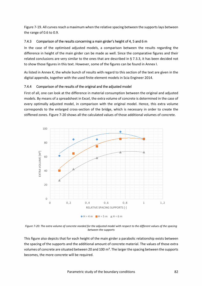
Parametric study of the boundary conditions 82
Figure 7-19. All curves reach a maximum when the relative spacing between the supports lays between
the range of 0.6 to 0.9.
7.4.3 Comparison of the results concerning a main girder’s height of 4, 5 and 6 m
In the case of the optimised adjusted models, a comparison between the results regarding the
difference in height of the main girder can be made as well. Since the comparative figures and their
related conclusions are very similar to the ones that are described in § 7.3.3, it has been decided not
to show those figures in this text. However, some of the figures can be found in Annex I.
As listed in Annex K, the whole bunch of results with regard to this section of the text are given in the
digital appendix, together with the used finite element models in Scia Engineer 2014.
7.4.4 Comparison of the results of the original and the adjusted model
First of all, one can look at the difference in material consumption between the original and adjusted
models. By means of a spreadsheet in Excel, the extra volume of concrete is determined in the case of
every optimally adjusted model, in comparison with the original model. Hence, this extra volume
corresponds to the enlarged cross-section of the bridge, which is necessary in order to create the
stiffened zones. Figure 7-20 shows all the calculated values of those additional volumes of concrete.
Figure 7-20: The extra volume of concrete needed for the adjusted model with respect to the different values of the spacing between the supports
This figure also depicts that for each height of the main girder a parabolic relationship exists between
the spacing of the supports and the additional amount of concrete material. The values of those extra
volumes of concrete are situated between 20 and 100 m³. The larger the spacing between the supports
becomes, the more concrete will be required.
0
20
40
60
80
100
0 0 , 2 0 , 4 0 , 6 0 , 8 1 1 , 2
EXTR
A V
OLU
ME
[M³]
RELATIVE SPACING SUPPORTS [-]
H = 4 m H = 5 m H = 6 m

Parametric study of the boundary conditions 83
Furthermore, one can also look at the figure concerning the additional volumes of concrete with
respect to the different heights of the main girder. For almost every value of the spacing between the
supports yields that the lower the height of the main girder is, the more concrete material is needed
to create the stiffened zone.
In a next step, the calculated values of the extra volume of the concrete, which are depicted in Figure
7-20 above, are divided respectively by the total volume of concrete regarding the original finite
element models. After that, those ratios are divided by the total length of the bridge, namely 175 m,
in order to obtain a global averaged relative value of the enlargement of a specific cross-section of the
bridge. Those determined values can be seen as a percentage in Figure 7-21.
All those percentages lay within a range of 2 to 9 %. Hence, the advantage regarding the material
consumption when one centrally placed main girder is applied instead of two girders, is reduced a
little. However, since the reduction in savings of the concrete material is rather small, this disadvantage
is negligible. In comparison with the original profit of saving a lot of concrete material when changing
the concept of the cross-section from two girders to only one main girder, the reduction of this
advantage due to the necessity of the additional stiffness, can be ignored.
The conclusions which can be postulated with respect to the relative values that are depicted in Figure
7-21, are very analogue to the ones that are highlighted regarding the values in Figure 7-20. One sees
again that parabolic regression-lines will arise with regard to the relationships between the different
parameters. Besides, the property of needing more concrete material with respect to the stiffened
zone, when the height h of the main girder decreases, yields once more.
Figure 7-21: The extra material needed for the adjusted model with respect to the different values of the spacing between the supports
0
2
4
6
8
10
0 0 , 2 0 , 4 0 , 6 0 , 8 1 1 , 2
EXTR
A M
ATE
RIA
L [%
]
RELATIVE SPACING SUPPORTS [-]
H = 4 m H = 5 m H = 6 m

Parametric study of the boundary conditions 84
Furthermore, the differences are studied between the parameters that are examined in detail in § 7.3
and the ones that are analysed in § 7.4.2 and § 7.4.3. In order to be able to compare easily the
differences with respect to the different heights of the main girder and/or the different values of the
spacing between the supports, all the differences are determined relatively with regard to the results
of the original models in Scia Engineer 2014. Moreover, the calculated ratios are given as percentages.
Since for all chosen heights of the main girder, the progresses of the relative differences of a specific
parameter with respect to the spacing between the supports are more or less uniform, another
simplification has been made in order to compare the differences in an easier way.
The calculated differences in the text below are all averaged values. For each parameter regarding a
certain spacing of the supports, the average of the three values according to the different values of h,
has been determined. Hence, the analyses and the results must be considered in a qualitative way and
certainly not in a quantitative way. In the case that one wants to know the quantitative values of the
relative differences in detail, those values can be viewed in the tables of Annex J.
Figure 7-22: Averaged relative difference of the reaction forces at the middle support with respect to the different values of the spacing of the supports
Figure 7-22 shows the relative differences between the values of the reaction forces at the middle
support with respect to the different values of the relative spacing. After a regression-analysis has been
executed, one finds a polynomial of the third order as the relationship between the spacing and the
relative differences. Both curves show a minimum or maximum respectively, in the case that the
relative spacing between the supports equals 0.3.
Moreover, in the case of large values of the relative spacing, the reaction force Zmin disappears almost
completely in the adjusted model. The differences regarding the reaction force Zmax are less explicit
-100
-80
-60
-40
-20
0
20
0 0 , 2 0 , 4 0 , 6 0 , 8 1 1 , 2
AV
ERA
GED
REL
ATI
VE
DIF
FER
ENC
E R
EAC
TIO
N F
OR
CES
[%
]
RELATIVE SPACING SUPPORTS [-]
Zmin,middle Zmax,middle

Parametric study of the boundary conditions 85
and circulate around 0 %. So, in that case the difference between the results of both models is
negligible.
In Figure 7-23 the values of the relative averaged differences regarding the reaction forces underneath
the other two supports are depicted. One can see that some of the calculated sets of results coincide.
Therefore, four different groups of relations are found, when a regression-analysis is executed. It has
to be noticed that all the differences of a specified reaction force regarding one support are almost
identical to the ones regarding the other support.
Two of the groups give rise to relationships between the differences and the spacing of the supports
as polynomials of the second order. Both types of parabolas start with values of the differences that
are rather small. In the case of the values with respect to Zmin, the curves decay when the spacing
between the supports increases. The differences are all negative. On the contrary, the curves regarding
the differences with respect to Zmax increase when the spacing of the supports enlarges.
Figure 7-23: Averaged relative difference of the reaction forces underneath track 1 and 2 with respect to the different values of the spacing between the supports
-15
-10
-5
0
5
10
15
20
25
0 0 , 2 0 , 4 0 , 6 0 , 8 1 1 , 2
AV
ERA
GED
REL
ATI
VE
DIF
FER
ENC
E R
EAC
TIO
N F
OR
CES
[%
]
RELATIVE SPACING SUPPORTS [-]
Xmin,track1 Xmax,track1 Ymin,track1 Ymax,track1 Zmin,track1
Zmax,track1 Xmin,track2 Xmax,track2 Zmin,track2 Zmax,track2

Parametric study of the boundary conditions 86
Furthermore, the curves that are polynomials of the third order are determined with regard to the
other two groups of relationships. It is remarkable that all four relations with respect to the reaction
forces in the X-direction at both supports underneath the tracks, coincide. The values of those
differences are never negative. Moreover, they all reach a maximum when the relative value of the
spacing between the supports is equal to 0.4. The latter is also the case with respect to the
relationships that are obtained for Ymin and Ymax. However, those maxima are smaller and the first part
of the curves gives rise to negative values of the averaged difference.
Figure 7-24: Averaged relative difference of the clamping moments with respect to the different values of the spacing of the supports
Besides, the averaged relative differences between the clamping moments around the longitudinal
and the vertical axis of the bridge, are examined. The progresses of those parameters are found in
Figure 7-24. There is a very slightly increasing linear relationship between the relative spacing of the
supports and the averaged differences of MX. In fact, those percentages are so small that the influence
on MX by the adjustment of the model, can be fully neglected. The latter is quite logical, because both
curves that are depicted in Figure 7-23 regarding the differences of Zmin and Zmax, are each other’s
reflection with respect to the horizontal line where the averaged difference equals zero.
In the case of the values regarding the differences that are determined for MZ, a polynomial of the
third order is found between those values and the ones of the relative spacing of the supports. The
shape of the curves is very similar or almost identical to the shape of the curves shown in Figure 7-23
regarding the differences of the reaction forces in the X-direction underneath both tracks. Again, a
maximum value of the difference is found in the case that the relative spacing equals 0.4.
Last but not least, in the tables of Annex J one can see that the difference between the original and
the adjusted model regarding the number of “strands B”, is rather small. The values are situated
-5
0
5
10
15
20
25
0,1
0,2
0,3
0,4
0,5
0,6
0 0 , 2 0 , 4 0 , 6 0 , 8 1 1 , 2
AV
ERA
GED
DIF
FER
ENC
E M
Z [%
]
AV
ERA
GED
REL
ATI
VE
DIF
FER
ENC
E M
X [
%]
RELATIVE SPACING SUPPORTS [-]
Mx,min1max2 Mxmin2max1 Mz,min1max2 Mz,min2max1

Parametric study of the boundary conditions 87
between 0 and 5 %. This can be clarified again by means of the Saint-Venant’s principle. Despite the
implementation of the extra stiffness at the start and end zone of the bridge, the greater part of the
adjustment of the cross-section of the bridge is concentrated just at the location of the boundary
conditions. Therefore, the principle remains valid and no large differences of the normal stresses at
the two restricted regions are visible.
Once again, all calculations and solutions with respect to the determination of the differences between
both models are found in a spreadsheet in Excel. As mentioned in Annex K, this spreadsheet is given
in the digital appendix.
7.5 CONCLUSIONS CONCERNING THE PARAMETRIC STUDY OF THE BOUNDARY CONDITIONS
In order to finish this chapter concerning the parametric study of the boundary conditions, some
general conclusions that can be postulated with respect to this specific research, are summarised in
the text below.
First of all, the research of the boundary conditions with respect to the original models in
Scia Engineer 2014 revealed two main problems. One of the problems dealt with the existence of
strange stress peaks regarding the stress distribution of the longitudinal normal stresses in the bridge
deck. The other problem concerned the exceeding of the requirement with respect to maximally
allowable value of the deck twist.
Eventually, it has been proven that both problems disappear by adding some extra stiffness to the
bridge deck over a specified length at the beginning and at the end of the bridge. The optimal length
of the stiffened zones increases when the height of the main girder decreases and its optimal thickness
shows a maximum when the value of the relative spacing between the supports lays between the
range of 0.6 to 0.9.
The consequences of adjusting the finite element model do affect the results of other parameters as
well. The latter seems to be very logical. However, not all parameters will respond in a same way to
those adjustments. Some of the parameters will have larger values, others will have values that have
decreased. There are even parameters for which the differences between the values regarding the
original and adjusted models, are negligible. For example, the magnitude of the clamping moments
around the longitudinal axis of the bridge will not change by implementing of the stiffened zone in the
finite element model.
Looking at the outcome of the implementation of a stiffened zone into the model, a disadvantage of
reducing the profit of saving concrete material by using one main girder instead of two main girders,
has been noticed. However, when both the original profit and the concrete material due to the addition
of stiffened zone are compared to each other, the overall sum of both contradictory material
quantities, gives rise to a net decrease of the material consumption. Hence, the advantage in terms of
material consumption with respect to the concept of an extradosed bridge with only one main girder
in a central position, still remains.
Furthermore, the way the selected parameters of the bridge change by altering the positions of the
supports of the bridge is totally in consensus with the principle of the Saint-Venant. Those alterations
only affect the results in the neighbourhood of the boundary conditions. For example, the obtained

Parametric study of the boundary conditions 88
results in the neighbourhood of the mid span remain unchanged while the model in Scia Engineer 2014
is adjusted.
Finally, as all calculated results and related conclusions with respect to the boundary conditions are
available now, the question can rise if there is an optimal position of the supports at both ends of the
bridge. Unfortunately, a balanced answer to this question cannot be given. Neither an optimal value
of the spacing between the supports, nor an optimal height of the main girder exists to minimise all
the reaction forces and the total amount of the concrete material, caused by the implementation of
the stiffening zone. An amelioration of one parameter results in a deterioration of another parameter
and vice versa.
Depending on the choices that have been made, the requirements that have been prescribed and the
significance that has been assigned to each parameter, other values with respect to the main girder’s
height h or to the spacing between the supports will become optimal. For example, when the total
amount of concrete is not governing in comparison with the total number of strands, the height h can
be chosen large in order to reduce maximally most of the reaction forces.
However, there are certain ranges with respect to the values of the spacing of the supports that have
to be avoided, regarding some specified parameters. For example, values of the spacing equal to 0 to
0.5 will give rise to extremely large vertical reaction forces regarding at the outermost supports
underneath the bridge deck, in comparison with the vertical reaction force at the support underneath
the main girder. Hence, in that case the design of the bearings will not be economical nor feasible
either.

Further research 89
FURTHER RESEARCH
In this next to last chapter, an overview is given of some subjects regarding the concept of an
extradosed railway bridge with one centrally placed stiffening girder that can be can be interesting to
analyse in the future. However, because of diverse reasons that will explained later on in this chapter,
those subjects are considered to be less important with regard to the scope of this master’s
dissertation. Therefore, they are not examined within this text. The subjects are as follows:
‒ A parametric study in order to search the optimal value of h and h1 when the ratio between L1
and L2 is altering;
‒ A parametric study of the boundary conditions that examines the influences on the stress
distribution and on other local parameters, when more than three supports at both ends of
the bridge are implemented;
‒ A parametric study of the boundary conditions that examines the influences of changing the
location of certain boundary conditions, for example the location where warping of the cross-
section is prevented, … on the stress distribution and on other local parameters;
‒ Analysing which part of “strands B” remains after having replaced it partially by usual post-
tensioned cables and other solutions in order to find a clear answer with respect to the
economic justification of this new concept;
‒ A parametric study that looks at the influences on the optimal number of strands when the
position of the main girder in the cross-section is altered vertically;
‒ Studying the influences on certain parameters when other span arrangements are used,
namely bridges with more than three spans, …;
‒ Studying this type of bridges with regard to motorised and pedestrian traffic
‒ Doing a research with respect to fatigue in the cables of this type of extradosed railway bridges;
‒ Analysing the second order effects and instability phenomena with regard to this type of
extradosed railway bridges, due to the use of more slender piers and a more slender cross-
section of the bridge.
All suggested analyses with respect to some local changes of the boundary conditions will not give rise
to significantly different results with respect to some global parameters as the total amount of cables,
the optimal height of the main girder, … . From Chapter 7 it is already clear that the Saint-Venant’s
priniciple will count if local adjustments are executed. Hence, for this first research on extradosed
bridges with one main girder, local studies will not influence the general conclusions a lot.
Furthermore, from the study on the search of possible cross-sections with one stiffening girder, it has
appeared that vertically altering the position of this girder in the cross-section of the bridge will not
result in a significant change of the global force distribution. Because of this, it is assumed that a more
detailed research on this matter will not give much more new general information.
Since one main goal of this research is to come up with a field of application of this type of bridges, a
research that deals with parametric studies of the cable tendon when the ratio of L1/L2 is adjusted, will
not contribute a lot to this goal. This possible subject will be interesting when one focuses more on a
specific side aspect of the bridge.

Further research 90
The part of the research with regard to instability phenomena is not discussed either, because most of
the time these phenomena will not be significant for the design of concrete structures. Therefore, one
thinks that despite the search for more slenderness, these phenomena will most probably not be
governing for this type of bridges.
Besides, the fatigue of the cables is not taken into account in this first general study on extradosed
railway bridges with one girder, because in an earlier master’s dissertation of extradosed bridges with
two main girders it appeared that one does not have to fear fatigue problems.
Last but not least, because the fixed time span of a master’s thesis, the presentiment of the non-
economical character of the bridge is not analysed more in detail. In the context of a first general
research on this type of extradosed railway bridges, the parametric study concerning the boundary
conditions has been assumed to be more interesting.

Final Conclusions 91
FINAL CONCLUSIONS
From all the results that are described in the previous chapters of this master’s dissertation, some
general conclusions can be put forward. Some of them have already been mentioned in the previous
sections of this text, but are so important that they are worth repeating in this part. Moreover, at this
moment one is also able to evaluate the main goals of this thesis, which are stated in § 1.2.
First of all, the concept of extradosed railway bridges with the stiffening girder in a central position
certainly has some significant advantages in terms of material consumption. In comparison with the
concept of extradosed railway bridges, where two main girders carry the main parts of the loads, this
new concept needs less concrete and the total required number of strands is strongly reduced as well.
However, the reduction of the concrete material that is caused by introducing a new type of cross-
section with respect to extradosed railway bridges, is somewhat neutralised by the need of stiffened
zones at both ends of the bridge. Those zones must be added to the bridge in order to overcome
problems with respect to the deck twist and to avoid detrimental, strange stress distributions inside
the bridge deck.
The decrease in consumption of both the concrete and the steel parts of the bridge will give rise to
another advantage. Since the needed quantity and hence the production of both materials is reduced,
this concept of bridges will be favourable for the environment because of a decrease of the emission
of CO2 among others.
Furthermore, this new type of cross-section concerning extradosed railway bridges, results in a visually
more attractive structure. Despite the increase in height of the main girder compared to the height of
the two main girders of the already known concept, the new bridge concept will look more slender.
Moreover, after having examined some local effects with regard to the boundary conditions and having
introduced the stiffened zones to the design of this the new concept, it appears that the assumed
substructure underneath the extradosed bridge will be feasible. Therefore, it is possible to make use
of the opportunity to build slender intermediate piers. This type of substructure will also contribute to
a better esthetical view of the bridge and to a reduction of the concrete consumption.
A substructure of the bridge, as mentioned in the previous section, gives rise to another advantage as
well. By using slender piers underneath the intermediate supports, a decrease of the total number of
bearings at those places can be realised. That reduction results in a decrease of the maintenance costs
and works during the lifetime of the structure.
In order to end this part of the conclusions with respect to the search of more slender elements to
obtain a visually more accepted structure, one important remark must still be mentioned. By increasing
the slenderness of the piers and the bridge deck, the resistance of those elements against accidental
loads or other extreme events will most probably decrease. So, due to this search of slenderness the
robustness of the global structure can diminish a lot.
Next, one can also look at the optimal values of some parameters regarding this concept of extradosed
railway bridges with the main girder in a central position. On the basis of all results mentioned in
previous chapters no real optimal value of the main girder’s height can be reached. In this context

Final Conclusions 92
“optimal” means a value of h that corresponds to a minimum of strands that are needed to counteract
the forces caused by the dead weight or LM71.
Depending on the span lengths of the bridge or in other words depending on the value of the scale
factor, a specified range of feasible heights of the main girder can be determined. The lower limit of
this range is found by taking into account the requirements with respect to the deformations that
follow from the passengers comfort demands. The upper limit is determined by considering the loading
gauge of the train and some visual criteria.
Eventually, within this range of heights, all the solutions will be acceptable from a structural and
esthetical point of view. Nevertheless, the higher the height is, the less strands are needed, but the
more concrete material has to be utilised.
Besides, it appears that an optimal value of the saddle height is even more difficult to determine than
an optimal value of the height of the main girder. Certainly in the case of larger main girder’s heights,
the differences between the values regarding the total number of strands, are so small that they almost
become negligible. Therefore, the height of the saddle can be chosen freely within a quite spacious
range, especially in the case of larger heights of the main girder.
An optimal positioning of the supports at both ends of the bridge does not exist either. Depending on
the selected parameter, another optimal value of the spacing between the supports will count.
However, when a certain set of parameters is viewed together and when those parameters are
classified according to their importance, ranges of the values of the spacing between the supports that
have to be avoided, can be determined.
Looking at all those conclusions with respect to the optimal values of certain parameters, one general
remark counts. The ultimate choice of a specific parameter of the bridge, will depend on the boundary
conditions that can be imposed by the local authorities, the public opinion or the economic
circumstances.
Furthermore, it is worth mentioning that all the useful relationships out of Chapter 6 between the scale
factors and some parameters, are linear. Moreover, it is even possible to determine the linear relation
between the scale factors and the multiplication that factors. The latter can be used to obtain easily
an estimation of the number of strands.
From Chapter 6 follows also that the calculated values of the ratios of the values of “strands B” relative
to the total number of the strands respectively, are situated between 70 and 76 %. This means that
the strands with respect to the cable tendon even do not represent one third of the total needed
amount of strands.
Of course, it must be taken into account that a part of those additionally placed strands can be avoided
by making use of the other solutions, see above. Another part of those centrally placed strands will in
reality be replaced by normal post-tensioned cables, which have a certain cable tendon inside the main
girder. Nevertheless, due to the rather big values of the ratios, there is a certain presentiment that this
concept is not so economical.
At the end of Chapter 3, a remark is postulated that the found optimal solution with respect to that
section resembles a normally prestressed beam. Fortunately, Figure 9-1 shows this is no longer the

Final Conclusions 93
case with regard to the bridge models in the further chapters. The reason for the view of the bridge in
Chapter 3 is probably due to all simplifications that have been made in that chapter in order to
determine quickly a cross-section with respect to this new concept.
Figure 9-1: Example of a sketch of one of the adjusted models from chapter 7
Last but not least, in the previous chapter an overview is given of some subjects regarding the concept
of an extradosed railway bridge with one centrally placed stiffening girder, which can be further
analysed. Those subjects are considered to be less important with regard to the scope of this master’s
dissertation. Some of them are left aside because other researched subjects seem to be much more
relevant and interesting with regard to the original goals of this master’s dissertation.

References 94
References
[1] K. K. Marmigas, „Behaviour and Design of extradosed bridges,” Toronto, 2008.
[2] M. Malfait, “Vermoeiingssterkte van extradosed voorgespannen zijdelingse brugliggers,” Gent,
2012.
[3] H. De Backer, Bridges II, Gent, 2014.
[4] L. Taerwe, Voorgespannen beton, Gent, 2013.
[5] Bureau voor Normalisatie, NBN EN 1992-1-1: Ontwerp en berekening van betonconstructies -
Deel 1-1: Algemene regels en regels voor gebouwen (+AC:2010), Brussel, 2005.
[6] Bureau voor Normalisatie, NBN EN 1992-1-1 ANB: Ontwerp en berekening van betonconstructies
- Deel 1-1: Algemene regels en regels voor gebouwen, Brussel, 2010.
[7] Bureau voor Normalisatie, NBN EN 1991-1-1 ANB: Belastingen op constructies - Deel 1-1 :
Algemene belastingen - Volumieke gewichten, eigen gewicht en opgelegde belastingen voor
gebouwen, Brussel, 2007.
[8] Bureau voor Normalisatie, NBN EN 1991-1-1: Belastingen op constructies - Deel 1-1 : Algemene
belastingen - Volumieke gewichten, eigen gewicht en opgelegde belastingen voor gebouwen (+
AC:2009), Brussel, 2002.
[9] Bureau voor Normalisatie, NBN EN 1991-2: Belastingen op constructies - Deel 2:
Verkeersbelasting op bruggen (+ AC:2010), Brussel, 2013.
[10] Bureau voor Normalisatie, NBN EN 1991-2 ANB: Belastingen op constructies - Deel 2:
Verkeersbelasting op bruggen, Brussel, 2011.
[11] Bureau voor Normalisatie, NBN EN 1990: Grondslagen van het constructief ontwerp, Brussel,
2002.
[12] Bureau voor Normalisatie, NBN EN 1990/A1: Grondslagen van het constructief ontwerp - Bijlage
A2: Toepassing voor bruggen (+ AC:2010), Brussel, 2013.
[13] K. Bruyland, „Parameterstudie van de Optimale Toepassing van Extradosed Naspanning in de
Bruggenbouw,” Gent, 2006.
[14] L. Vanhooymissen, M. Spegelaere, A. Van Gysel en W. De Vylder, Gewapend beton, Gent:
Academia Press, 2002.
[15] R. Van Impe, Berekening van Bouwkundige Constructies I, Gent, 2010.
[16] Bureau voor Normalisatie, NBN EN 1990 ANB: Grondslagen constructief ontwerp, Brussel, 2013.

References 95
[17] Infrabel, RTV KW01: Bouwen en instandhouding van kunstwerken: Bundel 1 - Bouwen van
kunstwerken en gebouwen, Brussel, 2012.
[18] R. Caspeele, Structural Analysis III, Gent: Department of Structural Engineering, 2014.
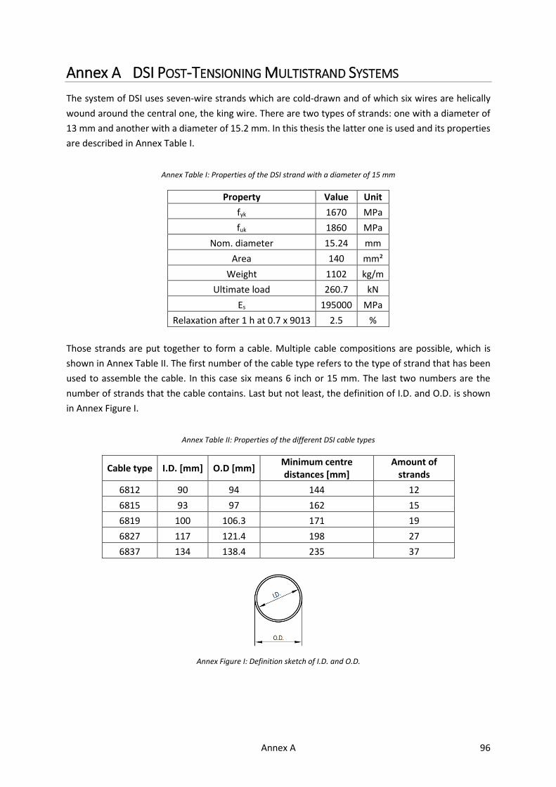
Annex A 96
Annex A DSI POST-TENSIONING MULTISTRAND SYSTEMS
The system of DSI uses seven-wire strands which are cold-drawn and of which six wires are helically
wound around the central one, the king wire. There are two types of strands: one with a diameter of
13 mm and another with a diameter of 15.2 mm. In this thesis the latter one is used and its properties
are described in Annex Table I.
Annex Table I: Properties of the DSI strand with a diameter of 15 mm
Property Value Unit
fyk 1670 MPa
fuk 1860 MPa
Nom. diameter 15.24 mm
Area 140 mm²
Weight 1102 kg/m
Ultimate load 260.7 kN
Es 195000 MPa
Relaxation after 1 h at 0.7 x 9013 2.5 %
Those strands are put together to form a cable. Multiple cable compositions are possible, which is
shown in Annex Table II. The first number of the cable type refers to the type of strand that has been
used to assemble the cable. In this case six means 6 inch or 15 mm. The last two numbers are the
number of strands that the cable contains. Last but not least, the definition of I.D. and O.D. is shown
in Annex Figure I.
Annex Table II: Properties of the different DSI cable types
Cable type I.D. [mm] O.D [mm] Minimum centre distances [mm]
Amount of strands
6812 90 94 144 12
6815 93 97 162 15
6819 100 106.3 171 19
6827 117 121.4 198 27
6837 134 138.4 235 37
Annex Figure I: Definition sketch of I.D. and O.D.

Annex B 97
Annex B EQUATIONS REGARDING THE CABLE TENDON
As stated before, the cable tendon calculations are done in case there is no equilibrium. To find the
independent parameters a progressive schema has to be applied [13]:
‒ Make a choice for the parameters a, u1, h1 and L1;
‒ Determine f1, b and i1 by means of equation ((26), (27) and (28);
𝑓1 =
ℎ − 𝑢1 −𝑎2
+ √(ℎ − 𝑢1 −𝑎2
)2
− (𝑎2
)2
2
(26)
𝑏 =4𝐿1𝑓1 + 𝐿1a + √(4𝐿1𝑓1 + 𝐿1a)2 − 16𝑓1𝑎ℎ1(𝑎 + 4𝑓1 + ℎ1)2
2 ∙ (𝑎 + 4𝑓1 + ℎ1) (27)
tan(𝑖1) =ℎ1
𝐿1 − 𝑏 (28)
‒ Choose a value for h2 and u2;
‒ Calculate now f2, c and i2 with equations (29), (30) and (31).
𝑓2 = ℎ − 𝑢2 (29)
𝑐 = 𝐿2
2𝑓2
2𝑓2 + ℎ2 (30)
tan(𝑖2) =4𝑓2
𝑐 (31)
The equation of the curved part of the cable tendon at the side span is given by the parabola k1. All
coefficients of equation (32) are given by formulas (33), (34) and (35).
𝑘1(x) = 𝑎1𝑥2 + 𝑏1𝑥 + c1 (32)
With:
a1 = −
𝑎 + ℎ1 −𝐿1𝑎
𝑏𝑏(𝑏 − 𝐿1)
(33)
b1 =
2𝑎 − ℎ1 −2𝐿1𝑎
𝑏𝑏 − 𝐿1
(34)
c1 = ℎ − 𝑎 (35)

Annex B 98
The equation of the curved part of the cable tendon at the mid span is given by the parabola k2. All
coefficients of this equation (36) are given by formulas (37), (38) and (39).
𝑘2(x) = 𝑎2𝑥2 + 𝑏2𝑥 + c2 (36)
With:
a2 =4𝑓2
𝑐2 (37)
b2 = −4(2𝐿1 + 𝐿2)𝑓2
𝑐² (38)
c2 =(2𝐿1 + 𝐿2)²𝑓2 + 𝑢2𝑐²
𝑐² (39)

Annex C 99
Annex C CROSS-SECTIONS OF THE BRIDGE FROM THE CASE STUDY
In this annex some of the used schema of the bridge of the case study can be viewed in Annex Figure
II, Annex Figure III, Annex Figure IV and Annex Figure V.
Annex Figure II: Cross-section of the extradosed railway bridge in Anderlecht
Annex Figure III: Longitudinal section of the extradosed railway bridge in Anderlecht
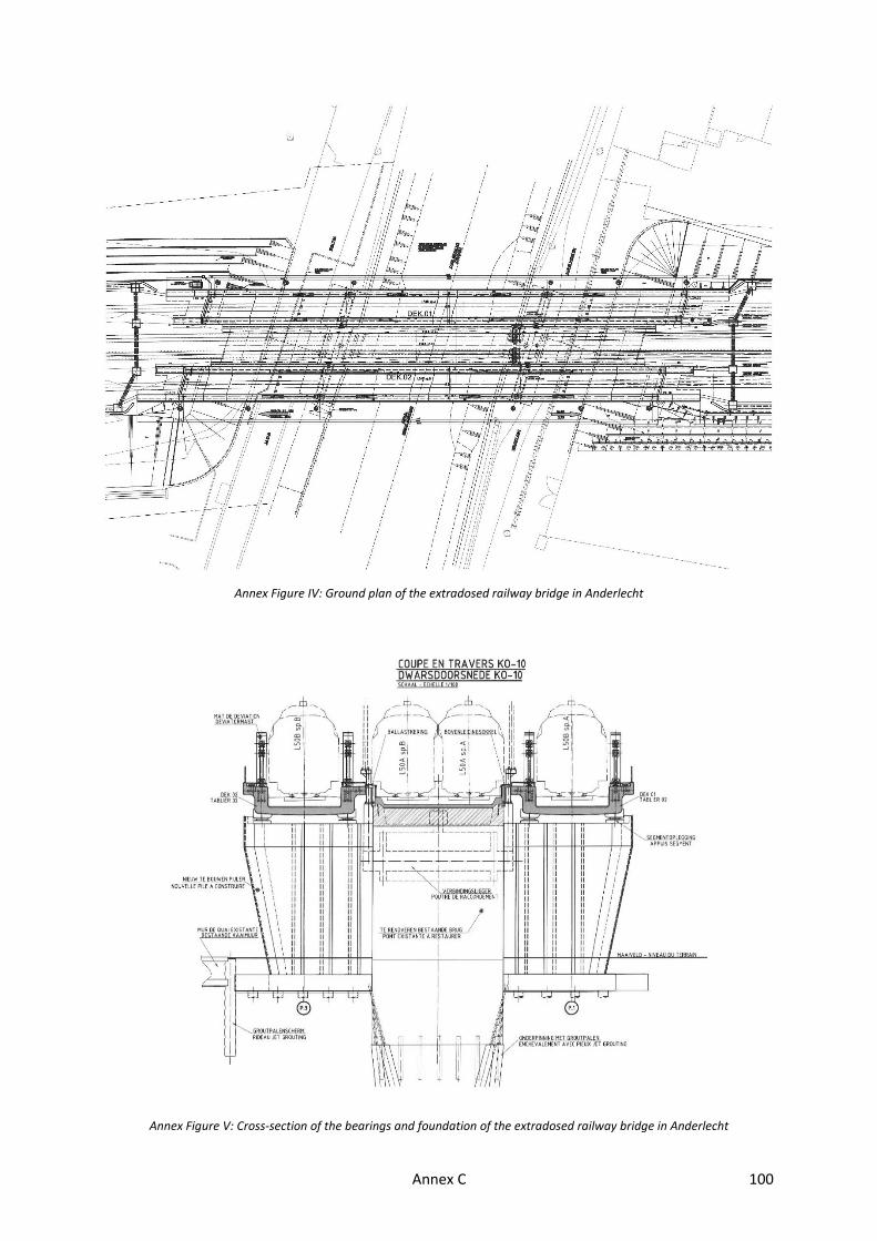
Annex C 100
Annex Figure IV: Ground plan of the extradosed railway bridge in Anderlecht
Annex Figure V: Cross-section of the bearings and foundation of the extradosed railway bridge in Anderlecht

Annex D 101
Annex D SCHEMAS OF THE CROSS-SECTIONS WITH TWO MAIN GIRDERS
Here the cross-sections of the different solutions with two main girders are given in Annex Figure VI,
Annex Figure VII, Annex Figure VIII and Annex Figure IX:
Annex Figure VI: Schema of B2-2000-1
Annex Figure VII: Schema of B2-2500-1
Annex Figure VIII: Schema of B2-2500-2
Annex Figure IX: Schema of B2-3000-1

Annex E 102
Annex E SCHEMAS OF THE CROSS-SECTIONS WITH ONE MAIN GIRDER
Here the cross-sections of the different solutions with one main girder are given in Annex Figure X,
Annex Figure XI, Annex Figure XII, Annex Figure XIII, Annex Figure XIV and Annex Figure XV:
Annex Figure X: Schema of B1-3000-1
Annex Figure XI: Schema of B1-3000-2
Annex Figure XII: Schema of B1-3250-1

Annex E 103
Annex Figure XIII: Schema of B1-4000-1
Annex Figure XIV: Schema of B1-4500-1
Annex Figure XV: Schema of B1-5000-1

Annex F 104
Annex F PROGRESSIVE SCHEMA TO ADJUST THE MODEL OF THE BRIDGE
This progressive schema in order to obtain an adjustment of the bridge, is split up into two parts. The
first one deals with all calculations in Excel, the second part gives rise to the implementation of the
calculations in Excel in the finite element program. All steps have to be executed chronologically. One
assumes that the determination of the most significant load cases has already occurred beforehand.
The calculations in Excel:
‒ Chose the parameters with respect to the cross-section and the cable tendon;
‒ Determine the position of the deviator saddle with respect to each by means of the solver;
‒ Chose the position of the support at both ends of the bridge;
‒ Now, all other characteristics of the model are automatically generated in different
spreadsheets.
Implementation of the calculated parameters in Scia Engineer 2014:
‒ Adjust the coordinates of the nodes;
‒ Change the magnitude of the forces;
‒ Change the cross-section of the cables in case this is necessary;
‒ Adjust the thickness of the 2D-elements if needed.

Annex G 105
Annex G RESULTS OF THE SCALED CASES
In this annex some of the results are given with regard to the calculations in Scia Engineer 2014 of the
scaled cases. The results with respect to each scaled case are grouped together.
Scale factor 1.5
Annex Figure XVI: Results search for an optimal value of h1 in case of different values of h
150
200
250
300
350
400
0 2 5 0 0 5 0 0 0 7 5 0 0 1 0 0 0 0 1 2 5 0 0
TOTA
L N
UM
BER
OF
STR
AN
DS
[-]
H1=H2 [MM]
H = 3 m H = 4 m H = 5 m H = 6 m

Annex G 106
Annex Figure XVII: Results search for an optimal value of h in case of different values of h1
Annex Figure XVIII: Optimal number of strands and their relative part of the strands B regarding the height of the main girder
200
225
250
275
300
325
2 5 0 0 3 0 0 0 3 5 0 0 4 0 0 0 4 5 0 0 5 0 0 0 5 5 0 0
TOTA
L N
UM
BER
OF
STR
AN
DS
[-]
H [MM]
H1 = H2 = 4000 mm H1 = H2 = 6000 mm
40
50
60
70
80
90
100
100
125
150
175
200
225
250
2 5 0 0 3 0 0 0 3 5 0 0 4 0 0 0 4 5 0 0 5 0 0 0 5 5 0 0 6 0 0 0 6 5 0 0
PA
RT
STR
AN
DS
B R
EGA
RD
ING
TH
E TO
TAL
NU
MB
ER O
F ST
RA
ND
S [%
]
TOTA
L N
UM
BER
OF
STR
AN
DS
[-]
H [MM]
Optimal amount of strands Percentage of the additional needed strands

Annex G 107
Annex Figure XIX: Optimal saddle height with respect to the height of the main girder
Scale factor 1.75
Annex Figure XX: Results search for an optimal value of h1 in case of different values of h
5000
6000
7000
8000
9000
2 5 0 0 3 0 0 0 3 5 0 0 4 0 0 0 4 5 0 0 5 0 0 0 5 5 0 0 6 0 0 0 6 5 0 0
OP
TIM
AL
SAD
DLE
HEI
GH
T [M
M]
H [MM]
200
225
250
275
300
325
350
0 2 5 0 0 5 0 0 0 7 5 0 0 1 0 0 0 0 1 2 5 0 0
TOTA
L N
UM
BER
OF
STR
AN
DS
[-]
H1=H2 [MM]
H = 4 m H = 5 m H = 6 m

Annex G 108
Annex Figure XXI: Results search for an optimal value of h in case of different values of h1
Annex Figure XXII: Optimal number of strands and their relative part of the strands B regarding the height of the main girder
225
250
275
300
325
350
3 5 0 0 4 0 0 0 4 5 0 0 5 0 0 0 5 5 0 0 6 0 0 0 6 5 0 0
TOTA
L N
UM
BER
OF
STR
AN
DS
[-]
H [MM]
H1 = H2 = 4000 mm H1 = H2 = 6000 mm H1 = H2 = 8000 mm H1 = H2 = 10000 mm
60
70
80
90
100
150
175
200
225
250
3 5 0 0 4 0 0 0 4 5 0 0 5 0 0 0 5 5 0 0 6 0 0 0 6 5 0 0
PA
RT
STR
AN
DS
B R
EGA
RD
ING
TH
E TO
TAL
NU
MB
ER O
F ST
RA
ND
S [%
]
TOTA
L N
UM
BER
OF
STR
AN
DS
[-]
H [MM]
Optimal amount of strands Percentage of the additional needed strands

Annex G 109
Annex Figure XXIII: Optimal saddle height with respect to the height of the main girder
Scale factor 2
Annex Figure XXIV: Results search for an optimal value of h1 in case of different values of h
6000
7000
8000
9000
3 5 0 0 4 0 0 0 4 5 0 0 5 0 0 0 5 5 0 0 6 0 0 0 6 5 0 0
OP
TIM
AL
SAD
DLE
HEI
GH
T [M
M]
H [MM]
200
250
300
350
400
450
0 2 5 0 0 5 0 0 0 7 5 0 0 1 0 0 0 0 1 2 5 0 0
TOTA
L N
UM
BER
OF
STR
AN
DS
[-]
H1=H2 [MM]
H = 4 m H = 5 m H = 6 m
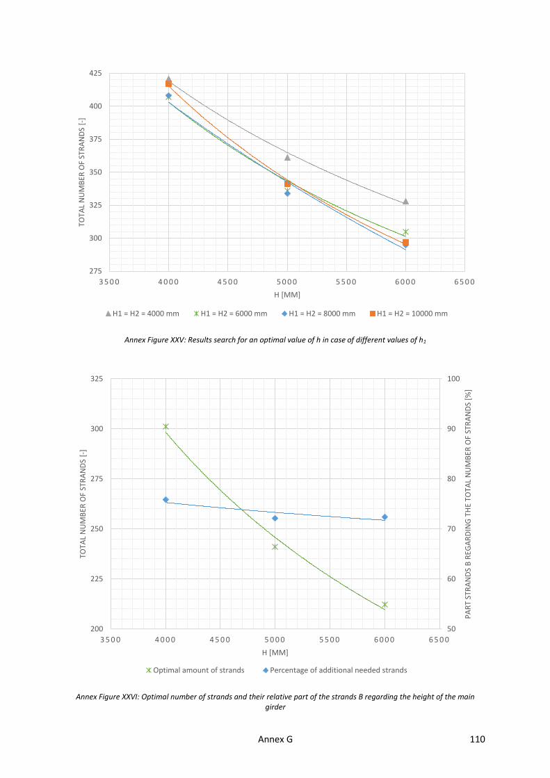
Annex G 110
Annex Figure XXV: Results search for an optimal value of h in case of different values of h1
Annex Figure XXVI: Optimal number of strands and their relative part of the strands B regarding the height of the main girder
275
300
325
350
375
400
425
3 5 0 0 4 0 0 0 4 5 0 0 5 0 0 0 5 5 0 0 6 0 0 0 6 5 0 0
TOTA
L N
UM
BER
OF
STR
AN
DS
[-]
H [MM]
H1 = H2 = 4000 mm H1 = H2 = 6000 mm H1 = H2 = 8000 mm H1 = H2 = 10000 mm
50
60
70
80
90
100
200
225
250
275
300
325
3 5 0 0 4 0 0 0 4 5 0 0 5 0 0 0 5 5 0 0 6 0 0 0 6 5 0 0
PA
RT
STR
AN
DS
B R
EGA
RD
ING
TH
E TO
TAL
NU
MB
ER O
F ST
RA
ND
S [%
]
TOTA
L N
UM
BER
OF
STR
AN
DS
[-]
H [MM]
Optimal amount of strands Percentage of additional needed strands

Annex G 111
Annex Figure XXVII: Optimal saddle height with respect to the height of the main girder
6000
6500
7000
7500
8000
8500
9000
9500
3 5 0 0 4 0 0 0 4 5 0 0 5 0 0 0 5 5 0 0 6 0 0 0 6 5 0 0
OP
TIM
AL
SAD
DLE
HEI
GH
T [M
M]
H [MM]

Annex H 112
Annex H RESULTS ORIGINAL MODELS RESEARCH BOUNDARY CONDITIONS
In this annex some of the results from the spreadsheet in Excel are given with regard to the research
of the boundary conditions on the original models in Scia Engineer 2014. The results of each height of
the main girder are grouped together.
Height of the main girder of 5 M
Annex Figure XXVIII: Values of the deck twist with respect to different values of the relative spacing
Annex Table III: Results of the reaction forces in SLS with respect to different values of the relative spacing of the supports
Relative spacing supports 0.1 0.25 0.5 0.75 1
Track 1
Xmin [kN] 1506.97 2694.50 2391.78 2304.54 1522.72
Xmax [kN] 1525.10 2735.94 2431.21 2341.05 1545.15
Ymin [kN] 178.09 258.55 380.62 588.86 473.01
Ymax [kN] 174.20 265.40 389.82 519.19 483.16
Zmin [kN] 19404.30 7488.80 3653.13 2425.85 1843.68
Zmax [kN] 20502.28 8484.61 4324.64 2884.58 2134.68
Middle Zmin [kN] 286.52 569.07 510.10 404.24 380.05
Zmax [kN] 3106.87 3644.97 4249.17 4575.13 4805.82
Track 2
Xmin [kN] 1525.59 2736.43 2431.70 2341.54 1545.64
Xmax [kN] 1506.49 2694.02 2391.29 2304.06 1522.24
Zmin [kN] 19341.40 7463.33 3640.17 2417.16 1837.18
Zmax [kN] 20569.12 8511.61 4338.01 2893.42 2143.24
0
2
4
6
8
10
12
14
16
18
20
0 0,2 0,4 0,6 0,8 1 1,2
DEC
K T
WIS
T [M
M/3
M]
RELATIVE SPACING SUPPORTS [-]

Annex H 113
Annex Figure XXIX: Reaction forces in Z-direction with respect to different values of the relative spacing of the supports
Annex Figure XXX: Moment around the longitudinal and vertical axis with respect to different values of the relative spacing
0
1000
2000
3000
4000
5000
0
5000
10000
15000
20000
25000
0 0,2 0,4 0,6 0,8 1 1,2
REA
CTI
ON
FO
RC
ES M
IDD
LE [
KN
]
REA
CTI
ON
FO
RC
ES T
RA
CK
1 A
ND
2 [
KN
]
RELATIVE SPACING SUPPORTS [-]
Zmin,track 1 Zmax,track 1 Zmin,track 2 Zmax, track 2 Zmin,middle Zmax,middle
19250
19350
19450
19550
19650
19750
0
4000
8000
12000
16000
20000
0 0,2 0,4 0,6 0,8 1 1,2
MO
MEN
TS M
X [
KN
M]
MO
MEN
TS M
Z [K
NM
]
RELATIVE SPACING SUPPORTS [-]
Mz,min1max2 Mz,max1min2 Mx,min1max2 Mx,max1min2

Annex H 114
Height of the main girder of 6 M
Annex Figure XXXI: The values of the deck twist with respect to different values of the relative spacing of the supports
Annex Table IV: Results of the reaction forces in SLS with respect to different values of the relative spacing of the supports
Relative spacing supports 0.1 0.25 0.5 0.75 1
Track 1
Xmin [kN] 1404.99 2439.50 2160.35 2093.58 1397.35
Xmax [kN] 1420.05 2473.85 2192.44 2123.13 1415.29
Ymin [kN] 456.96 236.22 346.26 463.96 436.27
Ymax [kN] 160.50 242.23 354.17 473.34 444.85
Zmin [kN] 19423.08 7495.77 3654.90 2426.61 1843.69
Zmax [kN] 20456.15 8471.03 4320.37 2882.28 2134.84
Middle Zmin [kN] 451.50 782.03 746.78 646.10 543.05
Zmax [kN] 2889.56 3397.35 3999.15 4325.24 4555.76
Track 2
Xmin [kN] 1420.94 2474.74 2193.33 2124.03 1416.18
Xmax [kN] 1404.09 2438.61 2159.45 2092.69 1396.46
Zmin [kN] 19351.35 7466.78 3640.18 2416.75 1836.32
Zmax [kN] 20531.84 8501.60 4335.50 2892.3 2142.29
0
2
4
6
8
10
12
14
16
18
20
0 0,2 0,4 0,6 0,8 1 1,2
DEC
K T
WIS
T [M
M/3
M]
RELATIVE SPACING SUPPORTS [-]

Annex H 115
Annex Figure XXXII: Reaction forces in Z-direction with respect to different values of the relative spacing of the supports
Annex Figure XXXIII: Moment around the longitudinal and vertical axis with respect to different values of the relative spacing
0
1000
2000
3000
4000
5000
0
5000
10000
15000
20000
25000
0 0,2 0,4 0,6 0,8 1 1,2
REA
CTI
ON
FO
RC
ES M
IDD
LE [
KN
]
REA
CTI
ON
FO
RC
ES T
RA
CK
1 A
ND
2 [
KN
]
RELATIVE SPACING SUPPORTS [-]
Zmin,track 1 Zmax,track 1 Zmin,track 2 Zmax, track 2 Zmin,middle Zmax,middle
19250
19350
19450
19550
19650
19750
0
4000
8000
12000
16000
20000
0 0,2 0,4 0,6 0,8 1 1,2
MO
MEN
TS M
X [
KN
M]
MO
MEN
TS M
Z [K
NM
]
RELATIVE SPACING SUPPORTS [-]
Mz,min1max2 Mz,max1min2 Mx,min1max2 Mx,max1min2

Annex I 116
Annex I RESULTS ADJUSTED MODELS RESEARCH BOUNDARY CONDITIONS
This annex contains some of the results from the spreadsheet in Excel with regard to the research of
the boundary conditions on the adjusted models in Scia Engineer 2014. The results of each height of
the main girder are grouped together. Furthermore, the figures that show some of the comparisons
between all the results are given as well.
Height of the main girder of 4 M
Annex Figure XXXIV: The values of the deck twist with respect to different values of the relative spacing of the supports
Annex Table V: Results of the reaction forces in SLS with respect to different values of the relative spacing of the supports
Relative spacing supports 0.1 0.25 0.5 0.75 1
Track 1
Xmin [kN] 1697.87 3578.80 3449.29 2898.57 1833.10
Xmax [kN] 1722.67 3647.77 3522 2960.95 1871.94
Ymin [kN] 174.67 290.14 474.50 571.72 499.96
Ymax [kN] 179.23 298.70 487.40 586.96 513.58
Zmin [kN] 19130.87 6999.02 3270.37 2082.83 1613.91
Zmax [kN] 20839.21 9029.25 4734.99 3252.38 2388.68
Middle Zmin [kN] 100.04 505.21 345.59 94.10 0
Zmax [kN] 2713.42 2904.74 3883.21 4456.9 4875.73
Track 2
Xmin [kN] 1723.04 3648.14 3522.37 2961.32 1872.31
Xmax [kN] 1697.50 3578.48 3448.90 2898.20 1832.73
Zmin [kN] 19073.77 6974.79 3258.05 2074.54 1607.61
Zmax [kN] 20901.59 9057.10 4748.95 3261.78 2395.58
2,5
2,7
2,9
3,1
3,3
3,5
0 0,2 0,4 0,6 0,8 1 1,2
DEC
K T
WIS
T [M
M/3
M]
RELATIVE SPACING SUPPORTS [-]

Annex I 117
Annex Figure XXXV: Reaction forces in Z-direction with respect to different values of the relative spacing of the supports
Annex Figure XXXVI: Moment around the longitudinal and vertical axis with respect to different values of the relative spacing
0
1000
2000
3000
4000
5000
0
5000
10000
15000
20000
25000
0 0,2 0,4 0,6 0,8 1 1,2
REA
CTI
ON
FO
RC
ES M
IDD
LE [
KN
]
REA
CTI
ON
FO
RC
ES T
RA
CK
1 A
ND
2 [
KN
]
RELATIVE SPACING SUPPORTS [-]
Zmin,track 1 Zmax,track 1 Zmin,track 2 Zmax, track 2 Zmin,middle Zmax,middle
19250
19350
19450
19550
19650
19750
0
5000
10000
15000
20000
25000
0 0,2 0,4 0,6 0,8 1 1,2
MO
MEN
TS M
X [
KN
M]
MO
MEN
TS M
Z [K
NM
]
RELATIVE SPACING SUPPORTS [-]
Mz,min1max2 Mz,max1min2 Mx,min1max2 Mx,max1min2
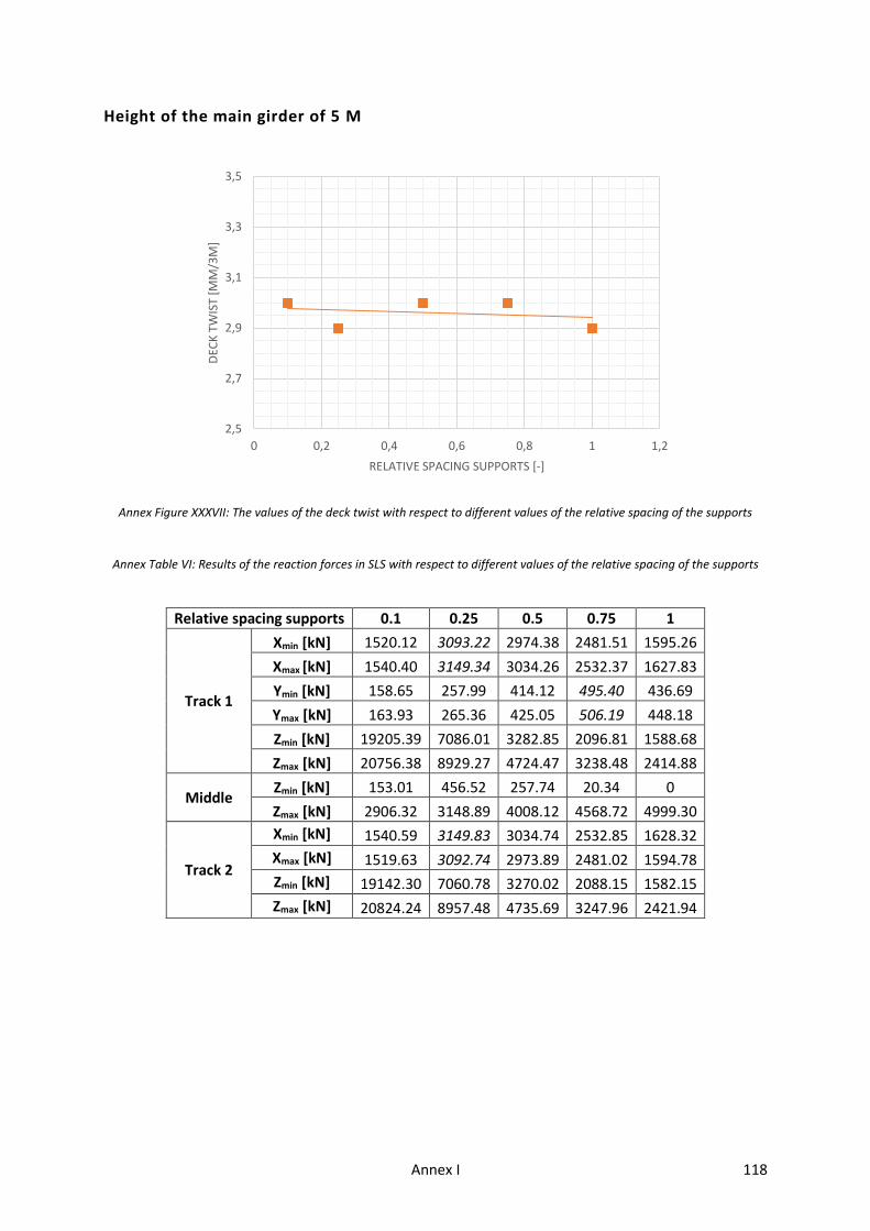
Annex I 118
Height of the main girder of 5 M
Annex Figure XXXVII: The values of the deck twist with respect to different values of the relative spacing of the supports
Annex Table VI: Results of the reaction forces in SLS with respect to different values of the relative spacing of the supports
Relative spacing supports 0.1 0.25 0.5 0.75 1
Track 1
Xmin [kN] 1520.12 3093.22 2974.38 2481.51 1595.26
Xmax [kN] 1540.40 3149.34 3034.26 2532.37 1627.83
Ymin [kN] 158.65 257.99 414.12 495.40 436.69
Ymax [kN] 163.93 265.36 425.05 506.19 448.18
Zmin [kN] 19205.39 7086.01 3282.85 2096.81 1588.68
Zmax [kN] 20756.38 8929.27 4724.47 3238.48 2414.88
Middle Zmin [kN] 153.01 456.52 257.74 20.34 0
Zmax [kN] 2906.32 3148.89 4008.12 4568.72 4999.30
Track 2
Xmin [kN] 1540.59 3149.83 3034.74 2532.85 1628.32
Xmax [kN] 1519.63 3092.74 2973.89 2481.02 1594.78
Zmin [kN] 19142.30 7060.78 3270.02 2088.15 1582.15
Zmax [kN] 20824.24 8957.48 4735.69 3247.96 2421.94
2,5
2,7
2,9
3,1
3,3
3,5
0 0,2 0,4 0,6 0,8 1 1,2
DEC
K T
WIS
T [M
M/3
M]
RELATIVE SPACING SUPPORTS [-]

Annex I 119
Annex Figure XXXVIII: Reaction forces in Z-direction with respect to different values of the relative spacing of the supports
Annex Figure XXXIX: Moment around the longitudinal and vertical axis with respect to different values of the relative spacing
0
1000
2000
3000
4000
5000
0
5000
10000
15000
20000
25000
0 0,2 0,4 0,6 0,8 1 1,2
REA
CTI
ON
FO
RC
ES [
KN
]
REA
CTI
ON
FO
RC
ES T
RA
CK
1 A
ND
2 [
KN
]
RELATIVE SPACING SUPPORTS [-]
Zmin,track 1 Zmax,track 1 Zmin,track 2 Zmax, track 2 Zmin,middle Zmax,middle
19250
19350
19450
19550
19650
19750
0
4000
8000
12000
16000
20000
0 0,2 0,4 0,6 0,8 1 1,2
MO
MEN
TS M
X [
KN
M]
MO
MEN
TS M
Z [K
NM
]
RELATIVE SPACING SUPPORTS [-]
Mz,min1max2 Mz,max1min2 Mx,min1max2 Mx,max1min2

Annex I 120
Height of the main girder of 6 M
Annex Figure XL: The values of the deck twist with respect to different values of the relative spacing of the supports
Annex Table VII: Results of the reaction forces in SLS with respect to different values of the relative spacing of the supports,
when H = 6 m
Relative spacing supports 0.1 0.25 0.5 0.75 1
Track 1
Xmin [kN] 1396.86 2738.15 2610.95 2149.25 1397.16
Xmax [kN] 1412.98 2782.78 2658.74 2189.19 1422.79
Ymin [kN] 150.44 236.54 370.62 437.85 398.14
Ymax [kN] 154.29 242.90 379.83 448.42 399.79
Zmin [kN] 19294.48 7188.80 3306.56 2117.96 1603.49
Zmax [kN] 20618.78 8810.50 4694.16 3215.34 2398.15
Middle Zmin [kN] 353.94 716.34 666.66 388.68 199.38
Zmax [kN] 2772.65 2952.02 3667.91 4206.51 4623.32
Track 2
Xmin [kN] 1413.88 2783.67 2659.75 2190.20 1423.80
Xmax [kN] 1395.97 2737.25 2609.94 2148.24 1396.15
Zmin [kN] 19222.63 7159.99 3291.91 2108.09 1596.03
Zmax [kN] 20695.10 8842 4710.05 3225.93 2406.03
2,5
2,7
2,9
3,1
3,3
3,5
0 0,2 0,4 0,6 0,8 1 1,2
DEC
K T
WIS
T [M
M/3
M]
RELATIVE SPACING SUPPORTS [-]

Annex I 121
Annex Figure XLI: Reaction forces in Z-direction with respect to different values of the relative spacing of the supports,
Annex Figure XLII: Moment around the longitudinal and vertical axis with respect to different values of the relative spacing
0
1000
2000
3000
4000
5000
0
5000
10000
15000
20000
25000
0 0,2 0,4 0,6 0,8 1 1,2
REA
CTI
ON
FO
RC
ES M
IDD
LE [
KN
]
REA
CTI
ON
FO
RC
ES T
RA
CK
11
AN
D 2
[K
N]
RELATIVE SPACING SUPPORTS [-]
Zmin,track 1 Zmax,track 1 Zmin,track 2 Zmax, track 2 Zmin,middle Zmax,middle
19250
19300
19350
19400
19450
19500
19550
19600
19650
19700
19750
0
5000
10000
15000
20000
25000
0 0,2 0,4 0,6 0,8 1 1,2
MO
MEN
TS M
X [
KN
L]
MO
MEN
TS M
Z [K
NM
]
RELATIVE SPACING SUPPORTS [-]
Mx,min1max2 Mz,min1max2 Mz,max1min2 Mx,max1min2

Annex I 122
Comparison between all the results
Annex Figure XLIII: Relative values of the reaction forces of the support under track 1 with respect to the height of the main girder
Annex Figure XLIV: Relative values of the reaction forces of the supports underneath track 2 and in the middle with respect to the height of the main girder
0,75
0,8
0,85
0,9
0,95
1
1,05
3 , 5 4 4 , 5 5 5 , 5 6 6 , 5
REL
ATI
VE
VA
LUES
REA
CTI
ON
FO
RC
ES [
-]
H [M]
Xmin,track1 Xmax,track1 Ymin,track1 Ymax,track1 Zmin,track1 Zmax,track1
0,75
0,8
0,85
0,9
0,95
1
1,05
3 , 5 4 4 , 5 5 5 , 5 6 6 , 5
REL
ATI
VE
VA
LUES
REA
CTI
ON
FO
RC
ES [
-]
H [M]
Xmin,track2 Xmax,track2 Zmin,track2 Zmax,track2

Annex I 123
Annex Figure XLV: Relative values of the clamping moments at the supports with respect to the height of the main girder
0,75
0,8
0,85
0,9
0,95
1
1,05
3 , 5 4 4 , 5 5 5 , 5 6 6 , 5
REL
ATI
VE
VA
LUES
CLA
MP
ING
MO
MEN
TS [
-]
H [M]
Mx,min1max2 Mx,max1min2 Mz,min1max2 Mz,max1min2

Annex J 124
Annex J RESULTS DIFFERENCES BETWEEN ORIGINAL AN ADJUSTED MODEL
In this annex the real relative values of the differences between the results of the selected parameters
regarding the original and the adjusted models, are given. All the differences are determined by means
of a spreadsheet in Excel By means of tables, the different percentages are grouped together regarding
the height of the main girder.
Height of the main girder of 4 M
Annex Table VIII: Values of the differences between parameters
Strands and stresses (SLS)
Relative distance supports 0.1 0.25 0.5 0.75 1
Distance supports 0 0 0 0 0
Hsaddle 0 0 0 0 0
H 0 0 0 0 0
1.19 2.38 2.38 3.57 2.38
-1.19 -1.19 -1.19 -1.19 -1.19
Strands cable 0 0 0 0 0
Strands extra 1.27 2.54 2.54 3.81 2.54
Total Strands 0.97 1.94 1.94 2.9 1.94
Reaction forces (SLS)
Track 1
Xmin 0.05 16.02 25.96 10.64 7.16
Xmax 0.25 16.4 26.43 11.15 7.72
Ymin -8.95 -1.21 6.9 -0.55 -5.47
Ymax -8.88 -0.99 9.8 -0.18 -5.03
Zmin -1.55 -6.61 -10.49 -14.13 -12.47
Zmax 1.67 6.44 9.48 12.72 11.74
Middle Zmin -74.43 -28.18 -47.59 -83.09 -100
Zmax -8.74 -16.75 -5.09 0.86 4.83
Track 2
Xmin 0.25 16.4 26.43 11.15 7.72
Xmax 0.11 16.02 25.96 10.64 7.16
Zmin -1.53 -6.63 -10.49 -14.17 -12.51
Zmax 1.65 6.44 9.47 12.71 11.72
Moments (SLS)
Mx,min 0.09 0.33 0.35 0.47 0.54
Mx,max 0.11 0.32 0.35 0.46 0.53
Mz,min 0.08 16.02 25.96 10.64 7.16
Mz,max 0.25 16.4 26.43 11.15 7.72

Annex J 125
Height of the main girder of 5 M
Annex Table IX: Values of the differences between parameters when h equals 5 m
Strands and stresses (SLS)
Relative distance supports 0.1 0.25 0.5 0.75 1
Distance supports 0 0 0 0 0
Hsaddle 0 0 0 0 0
H 0 0 0 0 0
1.64 3.28 3.28 4.92 4.92
-1.64 -1.64 -1.64 -1.64 -1.64
Strands cable 0 0 0 0 0
Strands extra 1.55 3.09 3.09 4.64 4.64
Total Strands 1.16 2.32 2.32 3.47 3.47
Reaction forces (SLS)
Track 1
Xmin 0.87 14.8 24.36 7.68 4.76
Xmax 1 15.11 24.8 8.17 5.35
Ymin -10.92 -0.22 8.8 -15.87 -7.68
Ymax -5.9 -0.02 9.04 -2.5 -7.24
Zmin -1.03 -5.38 -10.14 -13.56 -13.83
Zmax 1.24 5.24 9.25 12.27 13.13
Middle Zmin -46.6 -19.78 -49.47 -94.97 -100
Zmax -6.46 -13.61 -5.67 -0.14 4.03
Track 2
Xmin 0.98 15.11 24.8 8.17 5.35
Xmax 0.87 14.8 24.36 7.68 4.77
Zmin -1.03 -5.39 -10.17 -13.61 -13.88
Zmax 1.24 5.24 9.17 12.25 13
Moments (SLS)
Mx,min 0.14 0.27 0.34 0.48 0.59
Mx,max 0.14 0.26 0.37 0.47 0.63
Mz,min 0.87 14.8 24.36 7.68 4.76
Mz,max 0.99 15.11 24.8 8.17 5.35

Annex J 126
Height of the main girder of 6 M
Annex Table X: Values of the differences between parameters when h equals 6 m
Strands and stresses (SLS)
Relative distance supports 0.1 0.25 0.5 0.75 1
Distance supports 0 0 0 0 0
Hsaddle 0 0 0 0 0
H 0 0 0 0 0
0 0 2.17 2.17 2.17
-6.52 -6.52 -6.52 -6.52 -6.52
Strands cable 0 0 0 0 0
Strands extra 0 0 1.84 1.84 1.84
Total Strands 0 0 1.32 1.32 1.32
Reaction forces (SLS)
Track 1
Xmin -0.58 12.24 20.86 2.66 -0.01
Xmax -0.5 12.49 21.27 3.11 0.53
Ymin -4.12 0.14 7.04 -5.63 -8.74
Ymax -3.87 0.28 7.25 -5.26 -10.13
Zmin -0.66 -4.1 -9.53 -12.72 -13.03
Zmax 0.8 4.01 8.65 11.56 12.33
Middle Zmin -21.61 -8.4 -10.73 -39.84 -63.29
Zmax -4.05 -13.11 -8.28 -2.75 1.48
Track 2
Xmin -0.5 12.48 21.27 3.12 0.54
Xmax -0.58 12.25 20.86 2.65 -0.02
Zmin -0.67 -4.11 -9.57 -12.77 -13.09
Zmax 0.8 4 8.64 11.54 12.31
Moments (SLS)
Mx,min 0.09 0.21 0.33 0.47 0.59
Mx,max 0.09 0.21 0.32 0.46 0.58
Mz,min -0.58 12.24 20.86 2.66 -0.02
Mz,max -0.5 12.49 21.27 3.11 0.53
Annex K 127
Annex K OVERVIEW CONTENT DIGITAL APPENDIX
Below one can find an overview of all digital annexes that are given on the CD attached to this text:
‒ The spreadsheets regarding the solutions of the search for cross-sections with two main girders
and a comparison of those solutions;
‒ The Maple 18-files to determine the analytical equations regarding the internal forces;
‒ The Scia Engineer 2014-file to calculate the deformations and some geometrical properties
with respect to both types of cross-sections;
‒ The spreadsheets regarding the solutions of the search for cross-sections with only one
centrally placed main girder and a comparison of those solutions;
‒ The Maple 18-files to determine 𝜑 and its derivatives regarding the warping torsion;
‒ The spreadsheet with respect to a model in Scia Engineer 2014 with one cable tendon;
‒ The spreadsheet with respect to a model in Scia Engineer 2014 with two cable tendons;
‒ The models in Scia Engineer 2014 of the reference case;
‒ The models in Scia Engineer 2014 of the scaled case, namely scale factors 1.5, 1.75 and 2;
‒ The spreadsheet with the results of the parametric study of the reference case;
‒ The spreadsheet with the results regarding the selection process of the scale factors;
‒ The models in Scia Engineer 2014 to calculate the deformations regarding the selection of the
scale factors;
‒ The models in Scia Engineer 2014 of the scaled case, scale factor 1.5;
‒ The models in Scia Engineer 2014 of the scaled case, scale factor 1.75;
‒ The models in Scia Engineer 2014 of the scaled case, scale factor 2;
‒ The spreadsheet with the results of the parametric study of the scaled case, scale factor 1.5;
‒ The spreadsheet with the results of the parametric study of the scaled case, scale factor 1.75;
‒ The spreadsheet with the results of the parametric study of the scaled case, scale factor 2;
‒ The spreadsheet with the comparison between the results of the parametric study of the scaled
cases and the reference case;
‒ The spreadsheet regarding the calculation of the deck twist;
‒ The spreadsheet with the results of the parametric study of the boundary conditions with
respect to the original and the adjusted models in Scia Engineer 2014, for a main girder’s height
of 4 m;
‒ The spreadsheet with the results of the parametric study of the boundary conditions with
respect to the original and the adjusted models in Scia Engineer 2014, for a main girder’s height
of 5 m;
‒ The spreadsheet with the results of the parametric study of the boundary conditions with
respect to the original and the adjusted models in Scia Engineer 2014, for a main girder’s height
of 6 m;
‒ The spreadsheet with the comparison between all the results of the parametric study of the
boundary conditions, both for the original and the adjusted model, and the difference between
the results of both models;
‒ The different models in Scia Engineer 2014 in order to determine the deck twist and the normal
stresses with respect to the different values of the height of the main girder and of the spacing
of the supports.