external imbalances as an explanation for growth rate
TRANSCRIPT

Inaugural-Dissertation
zur Erlangung des Grades eines Doctor oeconomiae publicae (Dr. oec.publ.)
an der Ludwig-MaximiliansUniversität München
EExxtteerrnnaall IImmbbaallaanncceess aass aann EExxppllaannaattiioonn ffoorr GGrroowwtthh
RRaattee DDiiffffeerreenncceess aaccrroossss TTiimmee aanndd SSppaaccee::
An Econometric Exploration
vorgelegt von
Menbere Workie Tiruneh
Oktober 2003
Referent: Prof. Stephan Klasen, Ph.D. Korreferent: Prof. Dr. Dalia Marin Promotionsabschlussberatung: 11. Februar 2004

II
EExxtteerrnnaall IImmbbaallaanncceess aass aann EExxppllaannaattiioonn ffoorr GGrroowwtthh
RRaattee DDiiffffeerreenncceess aaccrroossss TTiimmee aanndd SSppaaccee::
An Econometric Exploration
By
Menbere Workie Tiruneh
Submitted to the Department of Economics
in partial fulfillment of the requirements for the degree of
Doctor oeconomiae publicae (Dr. oec. Publ.)
at the
Ludwig Maximilians University, Munich
2003
Thesis Supervisor: Prof. Stephan Klasen, Ph.D. Thesis Co-Supervisor: Prof. Dr. Dalia Marin Final Committee Consultation: 11. Februar 2004

I
Table of Contents
GENERAL INTRODUCTION........................................................................................ 1
I. GROWTH AND CONVERGENCE ACROSS TIME AND SPACE: NEW
EMPIRICAL EVIDENCE FOR AN OLD DEBATE.................................................... 7
1. INTRODUCTION ............................................................................................................. 9
2. THE SOLOW-SWAN MODEL AND THE CONVERGENCE DEBATE: A THEORETICAL REVIEW
....................................................................................................................................... 11
2.1. The absolute and relative convergence hypotheses ............................................ 13
2.2. Empirical specifications...................................................................................... 18
2.3. Review of previous empirical research ............................................................... 21
2.4. Data description and samples ............................................................................. 24
2.5. Results for cross-section regression and discussion........................................... 26
2.6. Conclusion........................................................................................................... 27
3. THE AUGMENTED SOLOW MODEL AND THE CONDITIONAL CONVERGENCE DEBATE:
REVISITING MANKIW, ROMER AND WEIL (1992) ........................................................... 28
3.1. The Textbook Solow Model ................................................................................. 30
3.2. The augmented Solow model and its empirical specification ............................. 31
3.3. Previous empirical studies on conditional convergence..................................... 34
3.4. Data description, results of the regression and discussion................................. 36
3.5. Conclusion and the policy implications .............................................................. 41
Bibliography............................................................................................................... 43
APPENDIX TO CHAPTER I. ............................................................................................... 46
II. AN EMPIRICAL EXPLORATION INTO THE DETERMINANTS OF
EXTERNAL INDEBTEDNESS .................................................................................... 75
1. INTRODUCTION ........................................................................................................... 77
2. WHY INDEBTED COUNTRIES GOT INDEBTED IN THE FIRST PLACE? A THEORETICAL
EXPLANATION ................................................................................................................. 79
2.1. What went wrong with the magnitude and structure of developing countries’
external debt? Some stylized facts.............................................................................. 87

II
2.2. Why HIPCs become HIPCs? Revisiting Easterly (2002).................................... 90
2.3. A further empirical exploration into the causes of LDCs external indebtedness in
the 1980s and 1990s................................................................................................. 104
3. CONCLUSION AND THE POLICY IMPLICATION OF THIS STUDY .................................... 113
BIBLIOGRAPHY ............................................................................................................. 115
APPENDIX TO CHAPTER II............................................................................................. 119
III. FACTORS AFFECTING THE DEBT-REPAYMENT CAPACITY OF
INDEBTED COUNTRIES: AN EMPIRICAL INVESTIGATION......................... 151
1. INTRODUCTION ......................................................................................................... 153
2. FACTORS AFFECTING DEBT-REPAYMENT CAPACITY: A THEORETICAL REVIEW ......... 155
3. A SUMMARY OF PREVIOUS EMPIRICAL STUDIES ........................................................ 158
4. ECONOMETRIC SPECIFICATION AND DATA DESCRIPTION ........................................... 160
5. DATA DESCRIPTION AND SAMPLES............................................................................ 163
6. RESULTS OF THE REGRESSION AND DISCUSSION........................................................ 163
7. CONCLUSION AND THE POLICY IMPLICATION OF THIS STUDY .................................... 166
BIBLIOGRAPHY ............................................................................................................. 168
APPENDIX TO CHAPTER III. .......................................................................................... 170
IV. DEBT OVERHANG, CAPITAL FLIGHT AND ECONOMIC GROWTH: A
PANEL DATA APPROACH....................................................................................... 179
1. INTRODUCTION ......................................................................................................... 181
2. THE EXTERNAL IMBALANCES-GROWTH NEXUS: A THEORETICAL REVIEW .............. 183
2. 1. A formal theoretical model of the debt overhang hypothesis.......................... 186
2.2. Capital flight, external debt and growth ........................................................... 190
2.3. The external imbalances-growth nexus: An extended empirical examination.. 194
2. 4. The Augmented Solow model: Revisiting Hadjimiachael and Ghura (1995) .. 196
3. A SUMMARY OF PREVIOUS EMPIRICAL STUDIES........................................................ 201
4. SPECIFICATION OF THE EMPIRICAL MODEL AND DATA DESCRIPTION ......................... 203
4.1. The advantages of a panel data over a simple cross-sectional approach ........ 203
4.2. A Formal specification of the empirical model................................................. 205
5. DATA DESCRIPTION AND SAMPLES............................................................................ 206

III
6. REGRESSION RESULTS AND THE POLICY IMPLICATIONS OF THIS STUDY..................... 208
BIBLIOGRAPHY ............................................................................................................. 215
APPENDIX TO CHAPTER IV. .......................................................................................... 220

IV
List of Tables, Graphs and Figures
Chapter I List of text tables 3. Economic growth, capital accumulation and population growth (1960-2000)..........................................36 List of text figures 1. Absolute convergence hypothesis .............................................................................................................15 2. Conditional convergence hypothesis .........................................................................................................17 3. Absolute and conditional convergence hypotheses ...................................................................................20 4. Evolving distribution, tending towards bimodal........................................................................................23 List of Appendix tables A. Tables for cross-section results 1960-2000 (all observations) 1. Definitions of the variables and their sources ...........................................................................................47 2. Descriptive statistics of all observations ...................................................................................................48 3. Annual growth rate of real GDP per capita ...............................................................................................48 4. Regression results ( β -convergence) ........................................................................................................49 5. Variance of real GDP per capita (σ -convergence) ..................................................................................50 6. Regression results (1960-69) .....................................................................................................................51 7. Regression results (1970-79) .....................................................................................................................51 8. Regression results (1980-89) .....................................................................................................................52 9. Regression results (1990-2000) .................................................................................................................52 10. Regression results (1960-2000) ...............................................................................................................53 11. Regression results (1970-2000) ...............................................................................................................53 12. Regression results (1980-2000) ...............................................................................................................54 B. Table for panel data results 1960-2000 (all observations) 13. Descriptive statistics (1960-2000) ...........................................................................................................54 14. Cross-section pooled results (1960-2000) ...............................................................................................55 15. Random and fixed effects results (1960-2000)........................................................................................56 C. Tables for cross-section results for developing countries alone (1960-2000) 16. Descriptive statistics (1960-2000) ...........................................................................................................57 17. Regression results (1960-2000) ...............................................................................................................58 18. Regression results (1970-2000) ...............................................................................................................58 19. Regression results (1980-2000) ...............................................................................................................59 20. Regression results (1990-2000) ...............................................................................................................59 21. Regression results (1960-69) ...................................................................................................................60 22. Regression results (1970-79) ...................................................................................................................60 23. Regression results (1980-89) ...................................................................................................................61 D. Tables for panel data regression results for developing countries alone (1960-2000) 24. Descriptive statistics (1960-2000) ...........................................................................................................62 25. Cross-section pooled regression results (1960-2000) ..............................................................................62 26. Random and fixed effects regressions results (1960-2000) .....................................................................63

V
E. Tables for panel regressions for HIPCs alone (1960-2000) 27. Descriptive statistics (1960-2000) ...........................................................................................................64 28. Cross-section pooled regression results (1960-2000) ..............................................................................64 29. Random and fixed effects regressions results (1960-2000) .....................................................................65 30. List of all countries included in the regressions ......................................................................................66 List of Appendix Graphs (growth of rates of real GDP per capita against log of initial real GDP per capita levels) Graphs (A1) to (A7) are for all observations A1. Regression line (1960-69) ......................................................................................................................67 A2. Regression line (1970-79) ......................................................................................................................67 A3. Regression line (1980-89) ......................................................................................................................68 A4. Regression line (1990-2000)...................................................................................................................68 A5. Regression line (1960-2000)...................................................................................................................69 A6. Regression line (1970-2000)...................................................................................................................69 A7. Regression line (1980-2000)...................................................................................................................70 Graphs (A8) to (A12) are only for developing countries A8. Regression line (1960-2000)...................................................................................................................70 A9. Regression line (1970-2000)...................................................................................................................71 A10. Regression line (1980-2000).................................................................................................................71 A11. Regression line (1990-2000).................................................................................................................72 Graphs (A13) to (A15) are for OECD countries (1960-2000) A12. Regression line (1960-2000).................................................................................................................72 A13. Regression line (1970-2000).................................................................................................................73 A14. Regression line (1980-2000..................................................................................................................73 Chapter II List of text tables 1.1. Some economic and social indicators for HIPCs and non-HIPCs (1980-98) .........................................81 2.1. Definitions of variables in the HIPC’s regression ..................................................................................93 2.2. Macroeconomic policy, financing, and external shocks: A comparison between HIPCs and non-HIPCs (1982-99).................................................................................94 List of text figure 3. The recycling of the petrodollar scheme ...................................................................................................84 Text graphs 1. Gross domestic savings and investment to GDP ratio of HIPCs (1970-99) ..............................................97 2. Resource balance to GDP ratio of HIPCs (1970-99).................................................................................97

VI
Appendix tables 1. Tables for HIPC’s indebtedness (cross-section) (1982-99) 2.3. Definitions of variables and their sources ............................................................................................109 2.4. List of countries included in the regressio............................................................................................120 2.5. Descriptive statistics (cross-section data).............................................................................................121 2.6. Descriptive statistics (panel data) .........................................................................................................121 2.7-2.19. Cross-section regression results ........................................................................................... 122-125 2.20-2.36.panel regression results ...................................................................................................... 125-128 2.37. Easterly (2002) results ................................................................................................................ 129-130 2. Tables for the regression results on the determinants of external indebtedness Annual cross-section (1982-99) 2.38. Annual cross-section results (all observations) ..................................................................................131 2.39. Annual cross-section results (all observations) ..................................................................................132 2.1. Tables for the regression results (Panel data) 2.40a. Descriptive statistics (all observations) ............................................................................................133 2.40b. Correlation matrix (all observations)................................................................................................133 2.40c. Correlation matrix (all observations) ................................................................................................134 2.41a. Random and fixed effects results (all observations) .........................................................................135 2.41b. Random and fixed effects results (all observations) .........................................................................136 2.42. Cross-section pooled results (all observations) ..................................................................................137 2.43. Differences in variables between HIPCs and non-HIPCs...................................................................138 2.44. Impact of variables on indebtedness...................................................................................................138 2.2. Determinants of indebtedness (HIPCs alone)-Panel data 2.45a. Descriptive statistics .........................................................................................................................139 2.45b. Correlation matrix ............................................................................................................................139 2.45c. Correlation matrix.............................................................................................................................140 2.46a. Regression results .............................................................................................................................140 2.46b. Regression results.............................................................................................................................141 Tables for the magnitude and structure of external debt A. The magnitude of external debt
A1. Total external debt stock (mil. USD)....................................................................................................142 A2. Share of each group in total developing countries’ external debt (%)..................................................142 A3. Total debt to GDP ratio (%)..................................................................................................................143 A4. Total debt to exports ratio (%)..............................................................................................................143 B. The cost of external debt B1. Total debt service to exports ratio (%)..................................................................................................144 B2. Interest payments to exports ratio (%) ..................................................................................................144 B3. Interest payments to GNP ratio (%)......................................................................................................145 C. The structure of external debt C1. The share of short term debt in total debt (%) ......................................................................................145

VII
C2. Total concessional debt (mil. USD)......................................................................................................146 C3. Concessional debt to total debt ratio (%) ..............................................................................................146 C4. Share of multilateral debt in total debt (%)...........................................................................................147 D. Other indicators of external balance sustainability D1. Reserves to total external debt (%) .......................................................................................................147 D2. External balance on goods and services (%GNP).................................................................................148 D3. Share of each group (region) in total portfolio equity inflows (%).......................................................148 D4. Gross domestic savings (% of GDP) ....................................................................................................149 D5. Gross domestic investment (% of GDP)...............................................................................................149 D6. Net resource flows and transfers for HIPCs and others ........................................................................150 Chapter III List of text tables 3.1. Arrears and rescheduling (% of total external debt and GNP) .............................................................154 List of appendix tables 3.2. Definitions of variables and their sources ............................................................................................171 3.3. List of countries included in the study..................................................................................................172 3.4. Descriptive statistics ............................................................................................................................173 3.5. Correlation matrix ...............................................................................................................................173 3.6. Regression results for cross-section pooled probit and logit models....................................................174 3.7. Regression results for the cross-pooled probit and logit models ..........................................................175 3.8. Regression results for the fixed effects logit model .............................................................................176 3.9. Regression results for the fixed effects logit model .............................................................................177 3.10. Marginal effects of the covariates ......................................................................................................178 Chapter IV List of text figures 1. The debt Laffer curve ..............................................................................................................................185 2. The link between capital flight, external debt, and growth......................................................................194 List of appendix tables 1. List of countries in the regression according to regional classifications .................................................221 2. List of countries in the regression according to debt classifications........................................................222 3. Definitions of the variables and their sources.................................................................................. 223-225 4. Descriptive statistics................................................................................................................................226 A. Random and fixed effects regressions results 5. Total debt stock and economic growth....................................................................................................227 6. Short term and long term debts and economic growth ............................................................................228

VIII
7. Concessional and non-concessional debts and economic growth............................................................229 8. Private debt and public debts and economic growth ...............................................................................230 9. Debts from the World Bank, IDA and IMF and economic growth .........................................................231 10. Bilateral and multilateral debts and economic growth ..........................................................................232 B. Cross-section pooled regression results 11. Total debt stock and economic growth..................................................................................................233 12. Short term and long term debts and economic growth ..........................................................................234 13. Private debt and public debts and economic growth .............................................................................235 14. Concessional and non-concessional debts and economic growth..........................................................236 15. Debts from the World Bank, IDA and IMF and economic growth .......................................................237 16. Bilateral and multilateral debts and economic growth ..........................................................................238 17. Impacts of variables on growth .............................................................................................................239 18-23. correlation matrices.................................................................................................................. 240-245

IX
Acknowledgements A doctoral thesis is seldom only one man’s work. First and for most, I am grateful to
Almighty God for the opportunities and the marvelous people he has prepared for me
during the course of my study in Germany. On Earth, Professor Stephan Klasen is left
without competition. In fact, this work would neither have started nor ended without
Professor Klasen’s professional guidance, direction, enthusiasm, encouragements, and his
personal involvement in all dimensions of my accommodation in Germany. I have learnt
a lot from our discussions. Moreover, I treasure his balanced judgment and would love to
thank him for standing by my side during the hardest personal crisis in my life. This is
hardly forgetable. In short, I remain to him a heavily indebted poor person. May
Almighty God bless him and his family!
I have also benefited from other members of the department. I am particularly thankful to
Dr. Wolff for his friendship and valuable comments and suggestions. I thank Carola and
Parvati for their friendship, concern on the progress of the work and for proof reading and
other technical help. I also appreciate Mrs. Seidl and Mrs. Moufid for their help in the
administrative matters. Katarina, Mark, Peter, and Andreas deserve my acknowledgement
for their friendship and help in searching for the relevant literature.
My gratitude and respect go to my mother, W/ro Sewnet Bezabih, for her love, endurance
and commitment in raising six of us alone after the sudden loss of our father, His
Eminence, Mergeta Workie Tiruneh, during our early ages. In the context a poor country
like my own, this must have been a nerve wrecking task. Thank you, Etalem.
I would also like to express my hearty gratitude to other excellent friends and relatives of
mine, too numerous to be mentioned here, for their prayers, words of encouragements,
and help during my stay in Munich. Thank you all for sharing my burdens and stresses.
I appreciate a 15 months scholarship from the GraduiertenKolegg in Postcolonial studies.
Nevertheless, I admit that all the errors and omissions in this work are purely mine

1
General Introduction During the period 1960-73, growth in Africa was more rapid than in the first half of the century…Since 1980, aggregate per capita GDP in sub-Saharan Africa has declined at almost 1 percent per annum. The decline has been widespread: 32 countries are poorer now than in 1980. Today, sub-Saharan Africa is the lowest income region in the world” (Collier and Gunning, 1999, p. 3) “The debt crisis can be studied as a problem in epidemiology. A powerful virus, high world interest rate, hit the population of capital importing developing countries in the 1980s. Some countries succumbed to the virus, having to reschedule their debt on an emergency basis, while others did not. And of those countries that arrived for emergency treatment, some recovered sufficiently to enter the period of quiet convalescence, while others are still suffering from febrile seizures in the IMF’s intensive care unit”, Sachs and Berg (1988, p. 1). “LDC (Less developed country) capital outflows have to be tackled as part of the solution to the debt problem, not as something that needs to be addressed only later. If capital flight is given a free ride in the caboose of LDC debt train, the train has little hope of making the station” (Morgan Guaranty (1986): in Lessard and Williamson, 1987, p. 244). The failure of developing countries, notably those in the sub-Saharan Africa, to manage
narrowing their income per capita gap with the developed and other developing nations is one
of the most serious challenges of the new millennium. Several empirical studies indicate the
phenomena of divergence in real income per capita across the world economy at large in the
past four decades. This implies that while richer countries continued to grow richer, the poor
counterparts continued to grow poorer, eventually increasing the dispersion of income per
capita across countries and over time. Such studies also point out that the magnitude of
divergence in income per capita was worst in the past two decades compared with the 1960s
and 1970s.
The income per capita divergence of sub-Saharan Africa from the rest of the world is
particularly alarming. The average growth in real per capita income that was around 2% in the
1960s, declined to nearly 1% in the 1970s, to nearly 0% in the 1980s and 1990s. The figures
turned even worse when one takes a longer time horizon. The average growth in real income
per capita during 1970-2000 and 1980-2000 were indeed negative. This is in contrast to the
average growth for the whole world of nearly 3% in the 1960s, 2% in the 1970s, 1% in the
1980s and 1990s.
Studies also indicate that during the past two decades SSA has virtually been outrun in all
essential economic and social indicators by other developing regions. This sluggish growth
performance has naturally been translated into high rate of poverty, poor education standard,
poor health conditions, political instability and civil wars, poor investment environment, poor
subsequent economic growth, and further internal and external imbalances. The joint impacts

2
of all these are stagnation in economic growth and development, creating a vicious circle or
self-reinforcing mechanism. The vicious circle is so strong and the elements that created the
circle are so interlinked to each other that breaking it at a single point has proved to be very
difficult in the past two decades.
While there is a widespread consensus on Africa’s marginalization and divergence, there are
differences when it comes to identifying the factors that may have accounted for the region’s
poor growth record. The mis-performance of Sub-Saharan Africa or „Africa‘s growth
tragedy“ as Easterly and Levine (2000) rightly put it, has been explained from various fronts.
The potential factors range from bad policies and external shocks (Hadjimichael and Ghura,
1995; and Rodrik, 1999, among others), to ethnic fractionalization (Easterly and Levine,
2000), to gender inequality in education (Klasen, 2002), and to geographic location (Sachs
and Warner, 1998), among others.
The justifications include that since Africa has failed to adopt and implement sound policies,
it is suffering from a subsequent stagnation in economic growth and development compared
to countries that exercised more friendly policies (Hadjimichael and Ghura, 1995, among
others). Others argue that by the virtue of Africa’s diversity in terms of ethnic structure, it is
hard to reach any consensus on the long-term development doctrines for countries in this part
of the world compared to countries in other regions with lower ethnic diversity (Easterly and
Levine, 2000). Therefore, countries that are ethnically more diverse tend to have distorted
policies compared with those that are ethnically less fragmented.
On the education front, Klasen (2002) argues that the growth rate of developing countries is
mainly attributed to gender inequality in education that retards intergenerational transmission
of knowledge, among other disadvantages, eventually punishes growth. His results indicate
that growth was higher in countries with low gender inequality and lower in countries with
higher gender inequality in education. From a different perspective, Sachs and Warner (1998)
blame the extraordinarily unfriendliness of nature to Africa compared to other developing
regions. They argue that most countries in Africa are landlocked, which does not allow them
to easily integrate into the global trade. Moreover, most of the countries in Sub-Saharan
Africa are located in the tropics, a fabulous environment for diseases to flourish and dramatic
soil deterioration. These are all potential explanations for growth rate differences across
various groups of developing countries.

3
The above explanations and others notwithstanding, there are, nonetheless, questions that
remained unanswered. The first problem in this respect is the negative and significant dummy
for Africa in most of the growth regressions, which virtually left Africa’s slow growth
problems unexplained. Second, Africa’s ethnic structure has not dramatically changed in the
1980s and 1990s compared to the decades earlier. Third, Sub-Saharan Africa is in the same
tropics today as it had been in the 1960s and 1970s and yet has much lower economic
performance. Fourth, Africa does not seem to be particularly suffering from gender inequality
problem compared to other developing regions and previous decades. Fifth, there had been no
dramatic migration of African inhabitants towards or away from the coast in the past two
decades to blame the density of the population as an explanation for poor growth performance
in the past two decades. Moreover, with the exception of a few countries, like Ethiopia, the
countries that are landlocked today had also been landlocked in the 1960s and 1970s.
Furthermore, there are many countries on earth that are landlocked but have enjoyed
sustainable long-run economic growth record.
In this dissertation I try to relate the “Africa’s growth crisis” to the debt crisis of the 1980s
and 1990s. There are several reasons behind linking Africa’s mis-performance to the debt
crisis.
First, the fact that the growth rate of the region has become much worse in the last two
decades, which are the decades of the debt crisis, may imply that the timing cannot be taken
as a mere coincidence. Rather, there is a legitimate suspect for the growth crisis to be strongly
linked to the debt crisis. Second, the cruel reality that 33 of the 41 countries classified by the
World Bank and IMF as heavily indebted poor countries (HIPCs) are located in this region
must provoke one to link the debt crisis to the economic growth crisis of Africa. For
illustration, HIPCs total external debt to GNP that was around 72% in 1984, jumped to 115%
in 1998 (Global Development Finance, 2000 (CD-ROM)). This huge external debt has been
accompanied by a large transfer of resources from this group to the developed world in the
form of debt service payments, which accounted 21% of their exports in 1982, though
dropped to 16% in 1998.
High external debt through the debt overhang, crowding out and destabilizing effects may
hamper economic growth and leads to low level of investment, and poor subsequent economic
growth. This seriously limits the indebted poor nations’ debt repayment capacity and may

4
increase the demand for further external debt and rescheduling. This may serve against the
creditworthiness of the indebted poor nations and prevent them from generating non-debt
creating resources in order to finance their investment projects. As Edwards (1986, p. 570)
concludes, “the level of the country risk premium increases with the level of foreign
indebtedness (i.e., debt-GNP ratio)”. Today, almost all the heavily indebted poor nations are
virtually cut off from the international financial markets and are instead heavily dependent on
the multinational financial institutions. That is why the IMF is often called the “watch dog”
and the “gate-keeper” of the international debt management (Nafziger W., 1993).
Third, apart from the above bottlenecks of a high external debt, there is additional impediment
of external debt on the growth of indebted poor nations via the capital flight. As Dooley and
Kletzer (1994) point out, “in the aftermath of the 1982 debt crisis economists were surprised
to learn that a large part of the borrowing of developing countries from international
commercial banks was not matched by unrecorded net imports of goods and services but
instead was matched by unrecorded private capital outflows from developing countries (p. 2).
In this respect, despite persisting measurement problems, the estimated capital flight from
Africa was around 39% of the private wealth of the region in 1990 compared to 14% for other
developing countries (Collier and Gunning, p. 7).
Finally, the fact that Africa’s growth performance continued to deteriorate despite two
decades of structural adjustment may indicate the region’s being caught in a poverty trap:
High external debt accompanied by capital flight and high debt service payments generating
low growth and more divergence, higher demand for external financing and rescheduling of
past contractual debt obligations. This is in fact, what has come to be known as ‘circular
financing’, where indebted poor nations are borrowing new loans from overseas at higher
interest rates to pay back old ones at lower interest rates, leaving the circle closed and poor
nations poor for ever.
To discuss the above issues, this dissertation has been split into four chapters:
The first chapter revisits the convergence debate using the recent Penn World Table database,
ranging from 1960-2000 and a panel data approach. Particular emphasis is given to the
position of the heavily indebted poor countries to account for the role of external debt in the
process of convergence (divergence).

5
In the second chapter, this dissertation empirically explores the causes of indebtedness. The
main motive is that the causes of the external indebtedness of developing countries and their
subsequent failure to meet their contractual debt obligations have been one of the heated
debates both in the academic circles, policy makers, and the broader international community
since the outset of the debt crisis in 1982. Using the World Banks’ Global Development
Finance, 2000 (CD-ROM) and the World Development Indicators, 2001 (CD-ROM)
databases, and employing both cross-section, cross-section pooled and random and fixed
effects approaches, this part investigates the determinants of external debt.
The third chapter, using cross-section pooled logit, probit and fixed effects logit models,
empirically explores the factors behind the debt repayment problems of the developing
nations in general and HIPCs in particular in the past two decades. From the viewpoint of
empirical strategy, the application of a panel data approach seems to be highly preferable, as it
allows to control for time-specific events that are linked to overseas borrowing, particularly
given the rapid changes in the global macroeconomic environment in the past years.
Moreover, this strategy helps to produce a more robust explanation by allowing to incorporate
country-specific factors as developing countries themselves are heterogeneous in terms of
their colonial heritages, geopolitical and strategic significance, and creditworthiness, all
affecting the level of indebtedness and the potential bargaining power to manage the
subsequent debt crisis.
The last chapter looks at whether external imbalances could be potential explanations for
growth rate differences across the developing world. Although there is a wide-ranging of
theoretical literature on this issue, there are only few empirical studies that show that there is
an inverse relationship between growth and external imbalances. Moreover, all empirical
studies on this area have focused on the impact of total external debt stock on growth of real
GDP per capita, controlling for the traditional factors that appear in all growth regression in
the framework of the augmented Solow model. The critical innovation of this dissertation is
the premise that total external debt stock is uninformative and rather masks important
information, and therefore, should be decomposed according to maturity and source
structures.

I. Growth and Convergence across Time and
Space: New Empirical Evidence for an Old Debate
8
Abstract This paper contributes to the ongoing convergence debate in several ways: First, using the recent
Penn World Table’s database (PWT 6.1), it shows the absence of the so-called absolute
convergence across the world economy at large in the past four decades. While the decade- by-
decade regressions indicate similar results, things seem to have worsened in the 1980s and 1990s.
One primary suspect in this regard is the debt crisis, which kicked off in 1982 after Mexico’s
official announcement in the same year that it was quitting to service its external debt. From this
time on, things started falling apart in developing countries and the debt crisis quickly turned into
a development crisis.
A separate regression for developing countries alone indicates the absence of unconditional
convergence across this group of countries. But, once we split countries into groups with similar
political, economic and institutional parameters (OECD, for instance), it appears that there is
evidence for unconditional convergence.
Third, turning to the conditional convergence debate, where both physical and human capital
accumulations are incorporated into cross-country regressions, the results seem to suggest that,
countries have experienced conditional convergence, hence poorer ones growing faster than their
richer counterparts. However, the cross-section strategy is concluded as insufficient for
international comparison of growth as it does not allow to control for time-specific and country-
specific factors, which leads to omitted variable problem, among other things. Therefore, using
random effects model and fixed effects model and cross-section pooled time series strategy, this
paper further investigates the growth-rate difference across countries and over time. The results
suggest that once we control for decade-specific and country-specific factors and the traditional
variables that always appear in the augmented Solow growth framework, the regressions
generate more plausible and robust results.The cooefficient on intial GDP per per capita become
larger and highly significant, reflecting, amonmg other things, that once we control for time
specific and country specific factors and the tradionional determinants of growth, it seems to
suggest that countries are close to their own steady states. Moreover, these strategies help to
control for the indebtedness dummy to control for the impact of external debt on the speed of
convergence.

9
1. Introduction Economists have always been concerned with variations in income and living standards
across time and space. One way of measuring the speed at which countries are moving
not only towards their own steady states but also towards the income per capita of other
countries goes back to Solow’s (1956) growth framework. In this framework, countries
with high savings rate and low population growth are predicted to experience higher per
capita income than those in the opposite camp (Solow, 1956), ceteris paribus. This
seminal work was quickly picked up by other economists and has therefore been the
subject of constant extension.
In general convergence in the context of economic growth is said to occur in a cross –
section of economies, if there is a negative relationship between the growth rate of
income and the initial level of income (Barro, 1991; Sala-i-Martin, 1994 and 1996a and
1996b, Barro and Sala-i-Martin, 1995). In other words, convergence takes places, in a
cross-section of economies, if poor economies tend to grow faster than wealthy ones,
implying that the poorer the economy the more quickly it will tend to grow over a long
time horizon, and vice versa. Similarly, Baumol (1994) defines convergence as a
tantamount diminishing in the degree of economic inequality among countries. Though
the above definitions remain valid throughout this paper, it turns out that there are
significant disputes among growth scientists regarding the theory of economic growth
and convergence.1
Although economists have been interested in investigating whether poor economies
remain poor for many years, while rich countries remain rich for generations, this was
hampered by absence of long-run time series data until the mid-1980s that the
convergence debate drew the attention of not only mainstream macroeconomic theorists
but also econometricians. There are mainly two reasons for the growing concern in the
convergence debate (Sala-i-Martin, 1996b, pp. 1019):
1 Advocates of the endogenous growth model and other development economists in fact reject the hypothesis of converegnce.

10
• First, the existence of convergence across economies was proposed as the main
test of the validity of modern theorists of economic growth. Moreover, estimates
of the speeds of convergence across economies were thought to provide
information on one of the core parameters of growth theory: the share of capital in
the production function,
• Second, in the mid-1980s a data set on internationally comparable GDP levels for
a large number of countries (the Penn World Tables) became available and this
new data set enabled empirical economists to compare GDP level across time and
space.
The convergence debate is also vital as it is concerned with the gaps in living standards
between countries, i.e, whether these gaps are narrowing or rather widening across
countries and over time (Pritchett, 1996). Sala-i-Martin (1996), and Barro and Sal-i-
Martin (1995), using β -convergence and σ -convergence concepts, elaborate the
convergence debate more broadly.2 Sala-i-Martin (1996, pp. 1025) points out that the
lack of convergence means that the degree of cross-country income inequality not only
fails to disappear, but rather tends to increase overtime (σ -divergence); and that
economies (nations) which are predicted to be richer a few decades from now are the
same countries (nations) that are rich today ( β -divergence).3 Moreover, despite the
persisting disputes among economists on the determinants of long-run growth, the
convergence debate has also enormous policy implications for policy makers both in the
developed and developing countries. One of the key questions in this regard is to what
extent external aid and debt helped countries to achieve accelerated economic growth,
hence allowing them manage narrowing the living standard gaps between the richest and
poorest part of the world.
2 β -convergence occurs if economies that are poorer are predicted to grow faster that richer ones. On the other hand, σ -convergence occurs if the disperision of income per capita across countries declines overtime. The two concepts are broadly discussed later in the paper. 3 See, Sala-i-Martin, (1994, 1996), and Barro and Sala-i-Martin (1995) for the detailed distinguishing between sigma and beta convergence.

11
The objective of this paper is to empirically test whether the income gap between poor
and rich countries of the world has narrowed or rather widened in the past four decades.
Particular attention will be paid to the position of the heavily indebted poor countries
(HIPCs) in the process of convergence (divergence) in the past four decades, with
especial emphasis on the last two decades, which capture the periods of debt and
financial crises and other spill over effects of the process of globalization. To translate
this aim into reality, I used both the absolute and conditional convergence hypotheses and
a fresh international data set (The Pen World Tables (PWT 6.1)) by A. Heston, R.
Summers, and B. Aten covering the period 1960 to 2000. The remainder of the paper is
organized as follows: part 2 presents the summary of the neoclassical production function
and the distincion between the absolute and conditional convergence hypotheses. Using
the PWT 6.1 data set, this section presents empirical evidence for absolute convergence.
Part three discusses the augmented Solow model and its empirical specifications. This
will be followed by data description and empirical results. The very last sub-section of
this part will present results and the policy implications of this study.
2. The Solow-Swan model and the convergence debate: A theoretical review
Almost all recent empirical researches on economic growth kick off from the Solow
growth framework. This paper will also first summarize the basic model before an
empirical counterpart to it is presented.
The Solow model is a closed economy framework, where output (Y) is a function of
input variables, such as labor (L) and capital (K). This can formally be written as:
( )LKFY ,= (1)
There are three basic assumptions that are linked to this model:
1. the production function in eq. (1) assumes positive and marginal products with
respect to each input variables.

12
0�KF
∂∂
, 0�LF
∂∂
; 02
2
�K
F∂, 02
2
�LF
∂∂
(1.1)
Equation (1.1) indicates that while each input variable contributes positively towards
boosting the output that is produced, its marginal productivity falls over time as more and
more of it is added, ceteris paribus.
2. the production function exhibits constant returns to scale, indicating a
proportionate increase in output as the result of changes in all input variables.
This can formally be written as:
( ) ( )LKFLKF ,., λλλ = , for all 0�λ (1.2)
3. the third assumption is referred to as the so called ‘Inada conditions’.
( ) ( )( ) ( ) 0limlim
limlim00
==
∞==
∞→∞→
→→
LLKK
LLKK
FF
FF (1.3)
The Inada conditions expressed in eq.(1.3) state that while production with the absence of
input variables is impossible, their excess abundance also make their marginal product
diminished over time, ceteris paribus. The assumption of constant returns to scale in eq.
(1.2) is also consistent with the balanced growth path along which capital and effective
labour grow at the same rate. It is also helpful to rewrite the production function in eq.(1)
in its intensive form:
( ) ( )kLfLK
LLKFY =��
���
�== 1,, (1.4)
where,
==LK
k capital –labour ratio; and
==LY
y per capita income
Now, the production function in eq.(1) can be written in its intensive form:

13
( )kfy = (1.5)
The change in the capital stock with a constant savings rate:
( ) KtLKFsKIK δδ −=−=•
,,. (1.6)
( ) kkfsLK δ−=•
. (1.7)
nkLK
tLK
k −=∂
��
���
�∂≅
••
( ) ( )knkfsk .. δ+−=•
(1.8)
Finally, the growth rate of k can be approximated as:
( ) ( )δγ +−==•
nkkfskk
k /. (1.9)
Following Barro and Sala-i-Martin (1995, pp. 22), the long-run growth rates in the
Solow-Swan model are determined entirely by exogenous factors. The fundamental
conclusion about long-run growth, therefore, is negative, simply because the long term
growth rates are independent of the savings rates and the level of the production function.
Nevertheless, the model is very important in providing us with sound information about
the transitional dynamics of growth, which indicates the per capita convergence of an
economy towards its own stead-state value or to the per capita incomes of a cross-section
of economies (Barro and Sala-i-Martin, 1995).
2.1. The absolute and relative convergence hypotheses
2.1.1. The absolute (unconditional) convergence
14
Following Barro and Sala-i-Martin (1995), eq. (1.9) implies that the derivative of Kγ
with respect to k is negative:
( ) 0/'. �kkk
fkfsk
k��
�
���
���
�−=∂
∂γ (1.10)
This implies that, ceteris paribus, smaller values of k are linked to larger values of its
corresponding growth ( Kγ ). This suggests (provided that countries have similar rate of
savings (s), growth of population (n), rate of depreciation (δ ) and production function)
that all economies have the same steady state values of k* and y*. Then, if the only
difference across countries is the initial capital per capita (k), the model predicts that
countries with less capital per capita tend to grow faster than those with relatively higher
level of capital per capita. Therefore, the hypothesis that nations with lower capital per
capita tend to grow faster than those with higher capital per capita without putting any
restriction is referred to as absolute (unconditional) convergence (Barro and Sala-i-
Martin, 1995).
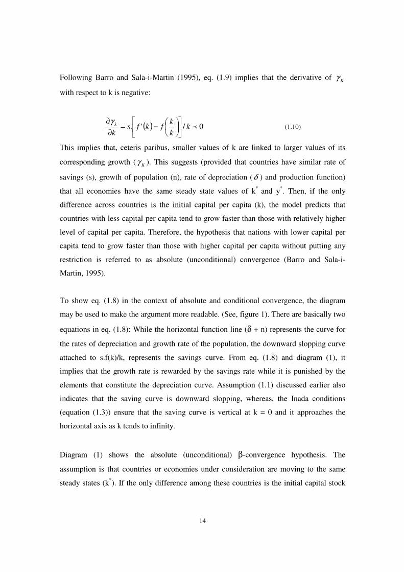
To show eq. (1.8) in the context of absolute and conditional convergence, the diagram
may be used to make the argument more readable. (See, figure 1). There are basically two
equations in eq. (1.8): While the horizontal function line (δ + n) represents the curve for
the rates of depreciation and growth rate of the population, the downward slopping curve
attached to s.f(k)/k, represents the savings curve. From eq. (1.8) and diagram (1), it
implies that the growth rate is rewarded by the savings rate while it is punished by the
elements that constitute the depreciation curve. Assumption (1.1) discussed earlier also
indicates that the saving curve is downward slopping, whereas, the Inada conditions
(equation (1.3)) ensure that the saving curve is vertical at k = 0 and it approaches the
horizontal axis as k tends to infinity.
Diagram (1) shows the absolute (unconditional) β-convergence hypothesis. The
assumption is that countries or economies under consideration are moving to the same
steady states (k*). If the only difference among these countries is the initial capital stock

15
(real GDP per capita), then poor regions are predicted to grow faster than rich economies
(∆kpoor >∆krich ). In other words, the growth rate of the poor towards the steady state is
predicted to be faster than the growth rate of the rich.
s.f(k)/k, (δ + n)
Figure (1). Absolute (unconditional) convergence Source: Sala-i-Martin (1996, pp. 1343: in Menbere, 2000)
Reasons in favour of the absolute convergence hypothesis include (Menbere, 2000):
• the first reason is that introduced by Baumol (1986), where he argues that there is
a common-force mechanism which assumes that at some stage circumstances
inherent in the growth process, a set of variables influences a number of
economies and drives them all in the same general direction. ”It is as though a
common terminal point (the steady state) is equipped with something analogous
to a magnet that draws toward itself all economies whose histories it affects”.
Following Baumol (1994),”the unusual thing about this magnet is that it exerts
the greatest force not on the economies closest to the terminal point but on those
that are farthest from it”. Hence, convergence occurs- the economies initially
farthest from the terminal (kpoor) are derived to move toward it most rapidly,
Growth Rate of Kpoor
Growth Rate of Krich
(n + δ)
Kpoor Krich K* Kt
s.f(k)/k (Saving curve)

16
which is a defining characteristics of a convergence hypothesis (in Baumol’s
terminology, a common-force convergence);
• since kpoor has lower level of initial capital (capital-labor ratio), any additional
investment would quickly push these economies towards the steady state, and
• although the above two reasons are based on the assumption that all economies
have similar economic parameters but different initial capital stock, there is a
third reason without the underlying assumption: The contagion model of
convergence predicts that because of contagion (say, imitation of production), the
laggards tend to grow faster than those in advanced stage of economic
development.4
Some arguments against the absolute ββββ- convergence hypothesis:
The core assumption of the absolute convergence hypothesis is that the sole difference
between nations is their initial levels of capital. The real world shows, however, that this
is just not the case. In fact, nations are different in so many other things, including the
level of technology, the propensity to save and natural endowments, among other things.
This is what has come to be known as the “absolute convergence fallacy”.
2.1.2 The relative (Conditional) Convergence hypothesis
The absence of broader empirical evidence in favor of absolute convergence across
economies makes the traditional absolute convergence hypothesis fruitless in terms of
measuring the speed of transition towards the steady state. Therefore, the idea of
conditional convergence has been introduced.5 As depicted in diagram (2) just below, if a
rich economy has higher saving rate relative to a poor economy (an assumption more
realistic than the previous one), then the rich economy might be proportionately further
from its steady state position. Under such circumstances, it should be the rich rather than
the poor economy that is predicted to grow faster towards its own steady state.
4 William Baumol, et al. (1994) ”Convergence of Productivity: Cross-National Evidence” Oxford Press Inc. 5 Conditional β-convergence exists if the partial correlation between growth and initial income is negative.
In contrast, a set of economies displays absolute β-convergence if the coefficient on initial income is negative in univariate regression (Sala-i-Martin,1996, p. 1330),.

17
s.f(k)/k, (δ + n)
Figure (2). Conditional (relative) Convergence Source: Sala-i-Martin and Barro (1995: in Menbere, 2000)
There are some more additional reasons against the absolute convergence hypothesis (or
in favour of the conditional convergence hypothesis) (Menbere, 2000):
• Poor economies have lower savings rate (due to lower income) compared to rich
ones and therefore, have lower rate of investment, and poor subsequent economic
growth,
• Rich countries as opposed to their poor counterparts have high growth rates,
despite their high initial capital-to-labor ratio, due to innovation,
• Ccapital is not moving from economies where it is abundant to those where it is
scarce, as was predicted by the contagion model of convergence, due mainly to
risk and uncertainty in most poor nations, and
(n+δ)
Kt
Growth Rate of Kpoor
Growth Rate of Krich
Kpoor K*poor Krich K*
rich
s.f(k)/k (Saving curve)
sf(k)/k (Saving curve)

18
• Finally, scarce qualified human capital in poor countries caused by both lack of
education as well as human capital flight (brain drain) makes the possible transfer
of technology and know-how from rich to poor countries slow and difficult.
2.2. Empirical specifications
The ββββ-Convergence hypothesis
The Solow-Swan growth model that allows measuring the coefficient of β, whose value
determines weather or not convergence has occurred in a cross-section of economies,
could be summarized as follows (see, Sala-i-Martin, 1996, p. 1334):
( )( )
( ) ( ) ,ln*1
ln
ln1,1,
1,
,titi
T
ti
ti YTe
Y
Y
Tµα
β
+��
�
� −−+=���
�
�−
−
−
(1.11)
Where,
α and β - are constants,
10 �� β , and µi, t is the error term with, and is assumed to have mean zero, same
variance ( 2µσ ) for all economies and is independent over time and across economies.
Then convergence occurs if β>0 and is statistically significant, as this implies the inverse
relationship between the annual growth rate ln (Yi,t/Yi, t-1) and the initial level of real per
capita income ln (Yi, t-1). Following Sala-i-Martin (1996), the coefficient on the initial per
capita level (1-e-βT)/T, which is the slope of the initial GDP per capita level, is an
expression that declines with the length of the time interval T for a given β. In other
words, if the linear relation between the growth rate of real GDP per capita and the initial
GDP per capita level are estimated, then the coefficient is predicted to be smaller the
longer the time period over which the growth rate is averaged. The reason is that the
growth rate declines as income increases. To calculate the β- coefficient from the
regression, one may linearize the model as follows:

19
���
����
� −−=−
Te
bTβ1 (1.11a)
The implied β that measures the speed of convergence may then be computed using the
following approximation (eq. 1.11b):
( )T
bT+−= 1lnβ (1.11b)
The σσσσ- convergence hypothesis
The second model has been developed to measure the cross-sectional dispersion of
income using sample variance of the log of income (σ- convergence)
( )[ ] =
−=N
ittiY
n 1
2,
2 ln1 µσ (1.12)
Where,
tµ - the sample mean of log of (Yi, t), and tiY , is the log of GDP per capita level of
country i at time period t. The main argument here is that if countries are converging in
terms of income per capita, the cross-sectional dispersion of their income should fall over
time.
At the outset of the empirical test for the convergence hypothesis, there was a heated
debate regarding the relationship between β-convergence and σ-convergence (apparently
first introduced by Sal-i-Martin). The central point of controversy was the presumption
that β- convergence be a necessary prerequisite for σ- convergence. The intuition behind
is that if there is convergence, the growth rate should fall over time (because when an
economy is getting richer, the predicted growth rate to be much smaller and vice versa).

20
However, later it was acknowledged that β- convergence is a necessary but not a
sufficient condition for σ- convergence to take place. This is either because of overtaking
or divergence. The first panel of diagram 3 indicates the absence of both β-convergence
and σ-convergence across economies, which implies that countries are diverging in terms
of their income per capita gap and this gap is increasing over time. In the second panel, it
is possible to notice that there is a decline in the income per capita gap between countries
and this was accompanied by a decline in the dispersion of income per capita across-
countries and overtime. The last panel seems to suggest overtaking or polarization, in
which case the middle class may vanish as Quah (1996) argues (more in a moment).
Absolute versus Relative Convergence in the Solow-Swan Model
Figure 3: Absolute and relative convergence Source: Xavier Sala-i-Martin (1996b), The Economic Journal, 106, pp. 1021
Log of (GDP)
t t t
A
B
A
B
A
B
Panel 1
Panel 2 Panel 3
β -Convergence = No σ - Convergence = No
β-Convergence = Yes σ-Convergence = Yes
β -Convergence = Yes σ -Convergence = No
1+T
T t+ T T
t+T T

21
2.3. Review of previous empirical research
Baumol (1986) has been the first growth economist to examine convergence across 16
industrialized countries (1870-1979) using Madison’s 1982 data. The results of the
regression suggest that there were perfect convergence across these groups of economies,
especially after World War II. De Long (1988) and Romer (1986) (in Sala-i-Martin,
1996b) demonstrate, however, that Baumol’s attempt in measuring convergence was
downplayed due mainly to the following:
• the first dispute is related to sample selection whereby historical data are
constructed retrospectively, the economies that have long data series are naturally
those that are more industrialized,
• Secondly, following the first reason, Baumol has been accused of biasedness. For
example, Quah (1996) criticizes the traditional empirical analysis growth and
convergence for overemphasizing physical capital and de-emphasizing
endogenous technological progress and externalities that are main determinants of
growth and convergence.
Similarly, Sala-i-Martin (1994, and 1996a), shows that β -convergence across the U.S,
Japan, and five European nations is strikingly similar (about 2 % per year).6 Based on the
above results, the author reaches two conclusions:
• Ffirst, the speeds of convergence are surprisingly similar across data sets, and
• Second, as the result of the first conclusion, since the degree to which national
governments use regional cohesion policies is very different, and the fact that the
speeds of convergence are very similar across countries implying that public
6 The results for 48 U.S. states from 1880-1920 indicate that dispersion of per capita personal income net of transfers declined from 0.54 in 1880 to 0.33 in 1920, then rose to 0.40 in 1930 due to the adverse shock to agriculture in 1920´s. The dispersion continued declining to 0.35 in 1940 and to 0.24 in 1960, to 0.17 in 1970 and 0.14 in 1976. The same observation for 47 Japanese prefectures for the period (1955-1987) of per capita income, shows that the dispersion of personal income increased from 0.47 in 1930’s to 0.63 in the 1940’s which was caused by explosion in military expenditure during that period. The cross-prefectual dispersion has decreased substantially since 1940: It fell to 0.29 by 1950, to 0.25 in 1960, 0.23 in 1970 and it hit a minimum of 0.12 in 1978. However, income dispersion was observed to constant since then (Sala-i-Martin 1996, pp. 1338).

22
policy plays a very small role in the overall process of regional convergence. This
has obvious been the subject of criticism by development economists and others
Nevertheless, as it is usual in economics, there is an ongoing serious dispute to the whole
debate of both the absolute and conditional convergences hypotheses. One of the most
serious criticisms comes from Danny T. Quah. Quah (1996a) interprets the neoclassical
definition of convergence as a “basic empirical issue, one that reflects - among other
things - polarization, income distribution, and inequality” (pp.1354). In an oversimplified
way, Quah links the convergence debate to the question of whether poor economies are
incipiently catching up with those already richer or instead they are caught in poverty
trap. In this regard, there are criticisms against the traditional convergence hypothesis,
which concludes that there exists a surprisingly similar 2% annual rate of convergence
across different countries.
Quah (1996a) argues that β -convergence is uninformative as it is interested only in
comparison of mean growth across countries but not in income distribution, and that
cross-section regressions can represent only average behaviour, not the behaviour of the
entire distribution (p. 1365). Moreover, Quah is concerned about the overall mission of
the convergence debate, according to him, as it fails to inform for instance “if the poorest
10% of the world are catching up with the richest 10% of the world”. He added that
studying an average economy or representative one gives little insight into the empirical
behaviour of the entire cross-section. He believes that for such cross-section dynamics to
be interpretable, one needs a theoretical model that makes predicitions on them (p. 1368).
His model then makes predictions on cross-section dynamics by taking three observations
(p. 1368): Countries endogenously select themselves into groups, and thus, do not act in
isolation; specialization in production allows exploiting economies scale; and ideas are an
important engine of growth.
From Quah’s hypothesis, two key results emerged: First, coalitions (convergence clubs) -
form endogenously - the model delivers prediction on coalition membership across the
entire cross-section of economies, and secondly, different convergence dynamics are

23
generated depending on the initial distribution of characteristics across countries. In this
potential dynamics explicit convergence clubs can be characterized as (Quah 1996, p.
1368): Polarization - the rich getting richer while the poor getting poorer and the middle
class vanishing (see also figure 4 below); stratification - when more than two coalition
form (multiple modes in the income distribution across countries); and overtaking and
divergence- two economies initially on roughly equal footing, separated over time so that
one eventually becomes wealthier than the other.
Figure 4: Evolving distributions, tending towards bimodal Source: Danny T. Quah (1996), European Economic Review 40 (p.1369), Numbers (1-4) added for explanation purposes.
Figure (4) provides the following interpretation of convergence:
1
2
3
4
T0 T1
Increasing income values
Income distribution
Time
24
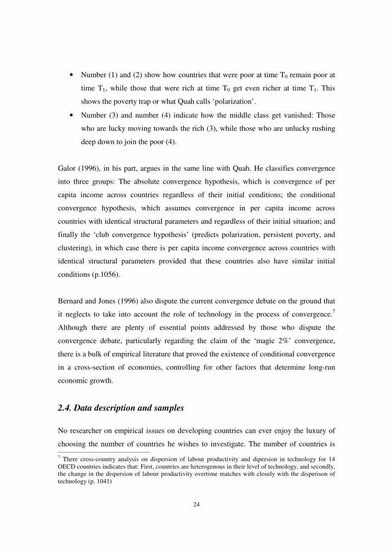
• Number (1) and (2) show how countries that were poor at time T0 remain poor at
time T1, while those that were rich at time T0 get even richer at time T1. This
shows the poverty trap or what Quah calls ‘polarization’.
• Number (3) and number (4) indicate how the middle class get vanished: Those
who are lucky moving towards the rich (3), while those who are unlucky rushing
deep down to join the poor (4).
Galor (1996), in his part, argues in the same line with Quah. He classifies convergence
into three groups: The absolute convergence hypothesis, which is convergence of per
capita income across countries regardless of their initial conditions; the conditional
convergence hypothesis, which assumes convergence in per capita income across
countries with identical structural parameters and regardless of their initial situation; and
finally the ‘club convergence hypothesis’ (predicts polarization, persistent poverty, and
clustering), in which case there is per capita income convergence across countries with
identical structural parameters provided that these countries also have similar initial
conditions (p.1056).
Bernard and Jones (1996) also dispute the current convergence debate on the ground that
it neglects to take into account the role of technology in the process of convergence.7
Although there are plenty of essential points addressed by those who dispute the
convergence debate, particularly regarding the claim of the ‘magic 2%’ convergence,
there is a bulk of empirical literature that proved the existence of conditional convergence
in a cross-section of economies, controlling for other factors that determine long-run
economic growth.
2.4. Data description and samples
No researcher on empirical issues on developing countries can ever enjoy the luxury of
choosing the number of countries he wishes to investigate. The number of countries is 7 There cross-country analysis on dispersion of labour productivity and dipersion in technology for 14 OECD countries indicates that: First, countries are heterogenous in their level of technology, and secondly, the change in the dispersion of labour productivity overtime matches with closely with the disperison of technology (p. 1041)

25
rather dictated by data availability. This also holds perfectly in this paper. The number of
countries ranges from 86 to 108, with their number varying from decade to decade and
variable to variable. The most troublesome variable is the Barro-Lee education data set,
where data is missing for a significant number of countries. I, therefore, used the log of
initial life expectancy alternatively. Since most HIPCs’ data on education is missing,
cross-country analysis was not possible. I, therefore, run a cross-section pooled time
series data using log of initial life expectancy for this group. The data for GDP per capita
and investment to GDP ratio were taken from the Penn World Table (PWT 6.1), an
expanded set of international comparisons, 1960-2000. Following the authors, “this data
displays a set of national accounts economic time series covering many countries. Its
expenditure entries are denominated in a common set of prices and in a common currency
(USD) so that real quantity comparison can be made, both between countries and over
time”. Data for life expectancy and population was taken from the World Development
Indicators (2001, CD-ROM). More information about the definitions and sources of the
variables that are used in the regression are in table (1). Table (2) presents the descriptive
statistics for the cross-sections of all observations. Table (13) presents descriptive
statistics for the panel data of all observations. Tables (16) and (24) present descriptive
statistics for cross-section and panel data regressions, respectively, for developing
countries alone. Table (27) show the descriptive statistics for HIPC’s pooled data.
Finally, table (30) shows the list of all countries that are included in the regression,
depending on data availability. In the decade-by-decade analysis, the averages were
calculated in a non-overlapping way: 1960-69, 1970-79, 1980-89, and 1990-2000.
Figures A1 to A15 in the appendix also show the regression lines that show the
correlation between log of GDP per capita growth and log of its initial value. Graphs A1
to A8 show the divergence (absence of absolute convergence) across all countries in the
world on decade-by-decade basis. Graphs A9 to A12 show the existence of rather
divergence across developing countries themselves. Graphs A13 to A15 show the
presence of absolute convergence across OECD members. While linear regression lines
indicate divergence (richer countries at the initial period experiencing higher average
economic growth), the inverse relations indicate convergence (those who were poorer at

26
the beginning of the observation period enjoying higher average economic growth). The
figures capture both for decade average regressions, the long-period averages, and across
different groups.
2.5. Results for cross-section regression and discussion
The results of the regression for absolute β -convergence are summarized in Tables (4).
The results for σ -convergence are in table (5). Table (3) presents annual growth rate of
real GDP per capital. The regression results in table (4) suggest that there was a
substantial divergence across the world economy at large in all the periods under
consideration when all countries were included in the regression (the values of β being
negative and statistically significant) indicating that there is a linear relationship between
Log of GDP per capita growth and initial Log of GDP per capita). In other words,
countries that were already rich in each initial period had also high annual growth rate
over the period in which it is averaged. This is consistent with the results of other
empirical studies including Sala-i-Martin (1991, 1996a and 1996b) and Barro and Sala-i-
Martin (1995), among others. Moreover, there is an evidence for σ -divergence (the
dispersion of income per capita increasing over time) during all the decades under
consideration. When all countries are included, the variance of income per capita
captured by σ 2 increased from 0.778 in 1960 to 0.948 in 1970; to 1.253 in 1980; to 1.483
in 1990; and to 1.704 in 2000. (See table (5)). When SSA countries were excluded from
the regression, the implied β-convergence become positive (except for the 1970-2000
period) though remains statistically insignificant, an indication of the absence of drastic
divergence across other developing countries relative to OECD countries. As one would
expect, Asia seems to have done quite well in narrowing the income gap with OECD,
though the situation worsened in the period 1990-2000, which obviously is linked to the
financial crisis many of the countries in the region have experienced during this period
This can also be seen from statistically significant coefficient of β, though things
worsened in the 1990s, and slightly declining dispersion in income per capita (σ -
convergence).

27
In contrast, there is a magnificent income divergence between SSA and OECD with the
strongest statistically significant values for β in all the periods that have been
investigated in this study. This is also supported by the poorest annual growth
performance of SSA (table 3) and high and increasing variance in income (an evidence
for σ-divergence). The income dispersion across OECD and SSA is drastic: the variance
of per capita income increased from 1.164 in 1960 to 1.416 in 1970; to 1.916 in 1980s; to
2.315 in 1990; and to 2.679 in 2000.
Though Latin America is slightly better than SSA, it has not either managed to
substantially narrow its income gap relative to OECD. The regression results for
developing countries alone suggest that there was divergence of per capita income
particularly in the last two periods (1980-2000 and 1990-2000). (See, graphs A9 to A12).
This is mainly attributed to the presence of outliers (East Asian countries) on the one
hand, and the severe external shocks Latin America and SSA have experienced during
these periods, on the other hand. As one would expect, there was a substantial progress in
narrowing the income gap across OECD countries, though the situation worsened during
the period (1980-2000). This again is linked to the recessions in most OECD countries in
the 1980s and the 1990s (see, graphs A13 to A15 in the appendix).
2.6. Conclusion
The empirical results so far indicate the following conclusions:
• Although there are disputes among economists regarding the measurement of the
speed at which the growth rates of different economies are approaching to each
other, there is no doubt that convergence has been a real world phenomenon in
regional groups with similar economic, institutional and political conditions and
convergence criteria (OECD and EU).
• The intensified divergence of the developing nations, notably those in Sub-
Saharan Africa, Latin America and South Asia may imply the failure of the

28
process of globalization to generate a proportionate benefit both for poor and rich
countries in the past two decades.
• The divergence of Sub-Saharan Africa implies, among other things, that since 33
of the 41 countries characterized by the World Bank and IMF as HIPCs are in
Sub-Saharan Africa, this may also suggest that the external shocks negatively
impacted on the region’s long term economic growth and overall development.
Having said that, however, since the quality of data for Sub-Saharan Africa has
been ranked by Alan Heston and Robert Summers as poor, the results of the
regression should be interpreted with caution.
• Finally, although the neo-classical growth model predicts convergence in the
sense that countries with lower initial capital-labor ratio are predicted to have
higher growth rates, it appears that this is only valid for moderately backward
countries that belong to a relatively advanced convergence club (poorer members
of OECD and EU) or for those countries that are well integrated into the global
economy through foreign trade and investment (East Asia).
3. The augmented Solow model and the conditional convergence debate: Revisiting Mankiw, Romer and Weil (1992)
The previous empirical investigation using the concepts of beta and sigma convergences
(see, tables (4) and (3)) clearly demonstrate interesting findings in the past four decades.
First, there was divergence in the cross-sections of the world economy at large
( )divergence−β and the per capita income dispersion across countries was increasing
overtime ( )divergence−σ . Second, there is an empirical evidence of income per capita
convergence across countries with relatively homogenous economic, political and
institutional parameters (OECD, for example), an empirical confirmation for the validity
of unconditional convergence. Third, the empirical results for developing countries alone
suggest that there was no absolute convergence across this group of countries despite
their heterogeneity in terms of per capita income. In contrast, rather there was a profound
degree of divergence particularly in the 1980s and 1990s. The greater degree of
divergence across developing countries in the past two decades is by no means a mere

29
coincidence, but could be the result of the debt crisis and other external shocks. This is
not, however, to discount the impacts of poor domestic policies and overall
mismanagement across the developing world.
Though there are seeds of truth in the previous analyses, there are some caveats that need
to be addressed to check the robustness of the results and the subsequent conclusion. The
first shortcoming of the previously discussed analyses is linked to selection biasedness
where countries are apriori chosen and put into groups based on similarities in their
economic, political and institutional parameters. The second caveat has something to do
with the empirical strategy that is employed in the convergence debate, which is based on
a cross-section analysis, which does not allow to control either for country-specific
events or time-specific factors that may affect countries’ growth performance and the
subsequent rate of convergence.8
To find a modest remedy to this issue, I have run several regressions, which include but
not limited to the following:
• The first attempt is to check conditional convergence in the spirit of the
augmented Solow model during the period 1960-2000, the longest period for
which data is available for the larger number of countries.
• Second, like in other similar studies, instead of apriori classifying countries into
groups, I incorporated initial life expectancy and education, alternatively, and
investment to GDP ratio to control both for human and physical capital
accumulations and initial GDP per capita to capture the conditional convergence
effect.
• Third, in the context of the above point, to check how the growth rate of
economies behaved during different decades, I decomposed the entire period into
decade averages. This has been done for the entire sample, developing countries,
and for HIPCs alone. The reason is that factors that affect developing countries
growth performance might differ from those that affect developed ones.
8 such issues have been broadly discussed by Islam (1995), Hoeffler (2000), among others.

30
• Fourth, switching to a panel data approach, I run both pooled cross-section time
series and random and fixed effects models. The main reason is that endogeneity
and omitted variable problems can not be solved in the cross-section framework.
The fixed effects model allows researchers on growth to control for time-specific
factors (decade-specific factors in this case) and country-specific factors that are
peculiar to the sample countries. Moreover, since the HIPCs dummy has always
been negative and significant in the cross-section approach, the model did not
explain the factors that account for HIPCs poor growth performance. As one of
the reasons for this to happen may be linked to the missing variables that may
determine the growth rate of this group but are not included, the fixed effects
model is used to take care of this problem.
3.1. The Textbook Solow Model
( ) ( ) αα −= 1)()( tLtAtKY (1.12)
10 ��α
Where, Y, K, A, L, and α stand for output, capital, the level of technology, labour, and
the share of capital in the production function, respectively. The model assumes that both
the growth rates of population and technology are exogenously determined. Therefore,
the level of technology and labor are expected to grow in the following ways:
gteAtA )0()( = (1.12a) nteLtL )0()( = (1.12b) ε+= aA )0ln( (1.12c)
The model also assumes that the number of effective units of labor, A(t)L(t), grows at
rate gn + .
Now, defining

31
ALY
y = is output per effective labour
ALK
k = is capital per effective labour
The evolution of k is determined by:
( ) ( )δ++−=• gnsytk (1.13)
= ( ) ( ) ( )tkgntsk δα ++− (1.14)
�
The steady state value of capital per effective labor,
� �
( )α
δ−
��
�
�
++=
11
*
gns
k ������������������������������������������������������������
�
Substituting equation (1.15) into the production function and taking logs, they arrived at
the steady state income per capita:
( )( ) ( ) ( ) ( )δ
αα
αα ++
−−
−++=��
�
����
�gnsgtA
tLtY
1ln
10lnln (1.16)
��
g+δ = assumed as constant across countries
A(0) = resource endowments, climate, institutions, etc.
lnA(0) = α + ε, where α and ε are a constant and country specific shocks respectively.
3.2. The augmented Solow model and its empirical specification
The augmented Solow model considers Cobb-Douglas production function, where output
(Y) is a function of both physical and human capital.
�βαβα −−= 1)(ALHKY ������������������������������������������������������������������
�

32
DefiningALH
h = , and leaving y and k as defined above, the production function in
intensive form can be written as:
βα hky = ��������������������������������������������������������������������������������������
The evolution of k and h, therefore, take the following form:
( )kgnysk k δ++−=•
������������������������������������������������������������������
( )hgnysh h δ++−=•
������������������������������������������������������������������
In the steady state, the levels of physical and human capital per effective labour are
constant. Thus, setting (1.2a) and (1.2b) to zero and solving the resulting equation gives
the following steady state values:
�
( ) ( ) βαββ
δ
−−−
��
�
�
��
�
�
++=
11
1*
gnss
k hk������������������������������������������������������������
( ) ( ) βααα
δ
−−−
��
�
�
��
�
�
++=
11
1*
gnss
h hk�����������������������������������������������������������������
Substituting (1.2c and 1.2d) into the production function (1.2/) and taking logs produces:
�
)ln(1
)ln(1
)ln(1
)0(ln)()(
ln hk ssgngtAtLtY
βαβ
βααδ
βαβα
−−+
−−+++
−−+−+=�
�
�
�����
��� ��
�
�
Measuring the speed of convergence
Following Mankiw, Romer, and Weil (1992), the Solow model makes quantitative
predictions about the speed of convergence to the steady state. Taking y* as the steady-
state level of income per effective worker given by equations (1.2c and 1.2d), and let y(t)

33
be the actual value at time t. Approximating around the steady state, the speed of
convergence is given by the following relationship:
�
[ ]))(ln()ln())(ln( * tyy
tty −=
∂∂ λ (1.4)
)1)(( βαδλ −−++= gn (1.5)
From equation (1.4), they move to a regression equation that measures the speed of
convergence.
))0(ln()ln()1())(ln( * yeyety tt λλ −− +−= (1.6)
Subtracting y(0) from both sides,
))0(ln()1()ln()1())0(ln())(ln( * yeyeyty tt λλ −− −−−=− (1.7)
Substituting for y*:
))0(ln()1()ln(1
)1(
)ln(1
)1()ln(1
)1())0(ln())(ln(
yegne
seseyty
tt
ht
kt
λλ
λλ
δβα
ββα
ββα
α
−−
−−
−−++−−
−−
−−−+
−−−=−
(1.8)
An empirical counterpart to (1.8) is given as:
))0(ln(.)ln(4.)ln(3.)ln(2.1))0(ln())(ln( ygnssyty hk ϕδβϕβϕβϕβ −++−++=−
(1.11)
where: te λϕ −−= 1
( ) εγδγγγβ +++++++=− ))0(ln(4)ln(3)ln(2ln(11))0(ln())(ln( yngssyty nk
(1.12) �
Where, [ ] ϕβ *)0(ln1 A=
The Hausman specification test for the random and fixed effects model

34
The Hausman specification test helps to decide whether it is the random effects model or
the fixed effects one that is more appropriate to be used. STATA provides with the
computed hausman for ∧
REβ (random effects model) and ∧
FEβ (fixed effects model),
where ∧
REβ and ∧
FEβ are consitent under the null hypothesis ( ) 0,:0 =itit XEH ε but this is
not happening if the null hypothesis does not hold. The ∧
FEβ is consistent regardless of the
null hypothesis. The ∧
REβ is BLUE, consistent and asymptotically efficient under the null
hypothesis, turn into inconsistent if the null hypotheisis fails to be true.
The Hausman test statistics is based on the differences between the estimated coefficients
on the two models (∧
REβ and ∧
FEβ ), whereby both models are equally specified. Then, the
Hausman test can be written as follows (Greene, 2003, among others):
(∧
FEβ -∧
REβ )/ [∧V {
∧}FEβ -
∧V {
∧
REβ }]-1(∧
FEβ -∧
REβ )
This under the null hypothesis is asymptotically distributed as 2Kχ , where K stands for
the degrees of freedom. STATA provides both the 2Kχ and its probability based on which
one can either opt for the random or fixed effects model.
3.3. Previous empirical studies on conditional convergence
Despite the disputes among economists, there is a bulk of empirical evidence on
conditional convergence across countries once the variables that affect the steady state
are controlled for. Barro (1991) is one the first in this regard, where using data for 98
countries in the period 1960-85, he shows that initial capital is negatively correlated with
the growth rate of GDP per capita, controlling for both human and physical capital

35
accumulation, and other policy variables. Human capital is believed to play a key role in
achieving accelerated economic growth from various fronts (Barro, 1991, p. 409).9
Mankiw, Romer and Weil (1992) tested the absolute convergence hypothesis using a
sample of 98 non-oil exporting countries, 75 intermediated countries and 22 OECD
countries in the period 1960-85. Their results indicate that the log of GDP per working-
age population is correlated positively with the investment and negatively with
population growth. Next, adding human capital accumulation to their model, while
population continues to have a negative impact on GDP per working-age person in 1985,
education and investment are positively correlated with GDP.
Here it is important to note two points: First, after controlling for education, the impact of
investment is now in line with the predictions. Second, once education is incorporated
into the regression, the explanation power of the model has jumped from 59% to 78% for
non-oil exporting countries. The jump in the R2 is quite high for the other groups as well.
Turning to the log difference in GDP per working-age (1960-85) as a dependent variable,
while they find an evidence for unconditional convergence across OECD, the remaining
groups have not demonstrated unconditional convergence. Finally, turning to the
augmented Solow framework, where schooling (a proxy for human capital accumulation)
was added, all groups have demonstrated conditional convergence and the overall
explanatory power of the model has improved substantially. Tsangarides (2000) using a
sample of 22 OECD and 42 African countries in the period 1960-90, indicates that while
9 Following Romer (1980, in Barro 1991), it is a fundamental input into the research sector, which is indispensable for technological progress. The empirical evidence also seems to suggest that countries with higher stock of human capital have a greater tendency to grow faster. As argued by Nelson and Phelps (in: Barro, 1991, p. 409), a larger stock of human capital also makes it easier for nations to imitate new ideas developed elsewhere. This gives the country that is a follower an enormous advantage to catch up relatively quickly towards those that are advanced. However, it appears that it is not only total education that matters for log-run economic growth. The quantity-quality trade offs and the distribution of education among men and women are issues that are on the agenda in recent empirical studies on economic growth and development. It seems that high total education if accompanied by gender inequality may not be extremely helpful for long-run economic growth. Klasen (2002) empirically shows that lower gender inequality may enhance economic growth through its direct externality effects (by feeding the economy with more educated labor force), and through its indirect externality effects, operating through demographic effects, lower gender inequality means higher education for women increasing the opportunity cost of women not to work and this leads to lower rate of fertility, which ultimately downsizes the population growth rate and increases capital deepening and growth, among other things.
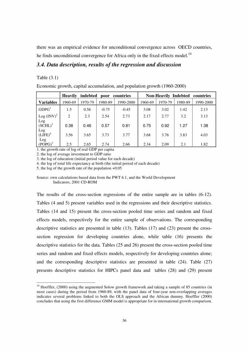
36
there was an empirical evidence for unconditional convergence across OECD countries,
he finds unconditional convergence for Africa only in the fixed effects model.10
3.4. Data description, results of the regression and discussion
Table (3.1)
Economic growth, capital accumulation, and population growth (1960-2000)
Heavily indebted poor countries Non-Heavily Indebted countries Variables 1960-69 1970-79 1980-89 1990-2000 1960-69 1970-79 1980-89 1990-2000
GDPG1 1.5 0.56 -0.75 -0.45 3.08 3.02 1.42 2.13
Log (INV)2 2 2.3 2.54 2.73 2.17 2.77 3.2 3.13 Log (SCHL)3 0.38 0.46 0.57 0.81 0.75 0.92 1.27 1.38 Log (LIFE)4 3.56 3.65 3.73 3.77 3.68 3.76 3.83 4.03 Log (POPG)5 2.5 2.65 2.74 2.66 2.34 2.09 2.1 1.82
1. the growth rate of log of real GDP per capita 2. the log of average investment to GDP ratio 3. the log of education (initial period value for each decade) 4. the log of total life expectancy at birth (the initial period of each decade) 5. the log of the growth rate of the population +0.05
Source: own calculations based data from the PWT 6.1, and the World Development
Indicators, 2001 CD-ROM
The results of the cross-section regressions of the entire sample are in tables (6-12).
Tables (4 and 5) present variables used in the regressions and their descriptive statistics.
Tables (14 and 15) present the cross-section pooled time series and random and fixed
effects models, respectively for the entire sample of observations. The corresponding
descriptive statistics are presented in table (13). Tables (17) and (23) present the cross-
section regression for developing countries alone, while table (16) presents the
descriptive statistics for the data. Tables (25 and 26) present the cross-section pooled time
series and random and fixed effects models, respectively for developing countries alone;
and the corresponding descriptive statistics are presented in table (24). Table (27)
presents descriptive statistics for HIPCs panel data and tables (28) and (29) present
10 Hoeffler, (2000) using the augmented Solow growth framework and taking a sample of 85 countries (in most cases) during the period from 1960-89, with the panel data of four-year non-overlapping averages indicates several problems linked to both the OLS approach and the African dummy. Hoeffler (2000) concludes that using the first difference GMM model is appropriate for in international growth comparison.

37
regression results for cross-section pooled time series and random and fixed effects
models, respectively for HIPCs. Finally Table (30) contains the list of countries that are
considered in the convergence analysis in this work.
Table (3.1) shows the differences in growth, investment, schooling, life expectancy, and
the growth rate of the population between HIPCs and non-HIPCs. The differences are
strikingly significant: The growth rate for HIPCs in the 1960s was about 1.5% compared
to around 3% for non-HIPCs counterparts. During this decade, HIPCs had quite
comparable figures in all the indicators in table (3.1). Although the growth rate failed to
0.56% in the 1970s, it seems that the worst was about to come. In fact, HIPCs, on
average, had negative growth rates throughout the 1980s and 1990s. What is even more
puzzling is that the deterioration in growth occurred despite improvements in investment
ratios, which puts both the quality of the data and investment under serious suspicion.
Now, turning to the results themselves, in regressions (6-12), while the average
investment to GDP ratio and initial education and initial life expectancy at birth, boost
income per capita growth; in contrast, the average growth rate of population, in most
cases, punishes it. The initial GDP per capita is inversely correlated with that of the
growth of GDP per capita, an indication of conditional convergence, holding investment,
education (life expectancy) and population growth rate constant. The results here are
generally consistent with the findings of most previous empirical studies.
My attempt in the framework of a cross-section regression was to figure out the extent to
which heavily indebted poor countries’ (HIPCs) growth performance had been deviating
from the other group of countries in the sample. In the first decade (1960-69, see, table
6), the HIPCs dummy was negative and significant perhaps indicating that this group of
countries had a relatively poorer growth performance during the decade while there was
a wide-spread growth across the world. Moving to the 1970s and 1980s (tables 7 and 8),
now HIPCs’ dummy became negative and relatively significant. In the 1990s, the
coefficient for this dummy was the highest in all the preceding decades and highly
statistically significant, reflecting among other things, the impact of the debt crisis to this
group during this decade. To capture the turbulence period of the 1980s and 1990s, I ran

38
the (1980-2000) log of GDP per capita growth against the 1980 log of real GDP per
capita, controlling for investment and education. The results indicate that this period was
in particular unfavorable to this group of countries. The coefficient on the initial log of
GDP per capita is also the lowest among all the other regressions. The longest period
(1960-2000, presented in table 10) also indicates the deviation of this group from the rest
of the countries in the sample.
HIPCs’ dummy did not change substantially even when I run separate regressions for
developing countries alone. In the first decade (1960-69), for instance, HIPCs did not
deviate too much from the rest of the developing world (table 21). While the 1970s and
1980s were quite unfavorable for this group, the 1990s seem to be even worse for HIPCs
as a whole, where there is an indication of a dramatic lag in terms of economic growth
(table 20). The longest period regression (1960-2000) also indicates that this group of
countries, on average, has the lowest economic growth relative to the rest of the world
during the entire past 40 years.
Switching to the panel data analysis, the first attempt was to run a cross-section pooled
time series regression for all observations (see table 14). The result now indicates that
while all the variables remain as in the previously discussed cross-section regressions,
HIPCs continues to have experienced a more sluggish economic growth as opposed to the
rest of the countries under investigation in this study. It is also interesting to note the
coefficients on the decade dummies included to capture decade-specific factors that may
hinder economic growth. The results seem to suggest that while the 1960s is the most
favorable decade, followed by the 1970s, the remaining two decades, the 1980s and
1990s were very poor ones for growth performance. It is also equally important to note
that the whole explanatory power of the regression has now increased after the inclusion
of the HIPCs’ and decades’ dummies relative to the simple cross-section regression that
was discussed earlier. The R2 in every regression where HIPCs dummy is included is
higher than when it has dropped.
Similarly, staying further in the spirit of the panel data approach, while the random
effects model generates almost similar results as that of the cross-section pooled time

39
series regression, the fixed effects model results confirm that the 1980s were harsh for
HIPCs.11 Isolating developing countries from the developed ones, the cross-section
pooled time series regression (table 25) indicates that while they all were doing well in
the 1960s and 1970s, things had changed for the worse in the 1980s, which got even
worse in the 1990s. Moreover, HIPCs themselves have experienced a drastic
deterioration in economic growth during these decades (see also table 3.3). The fixed
effects model again confirms that the 1980s were in fact the worst period for developing
countries as a whole.
The fact that the HIPCs dummy was always significant and negative does indicate the
problem of the augmented Solow model in explaining why some countries remain poor
while others remain rich. Other empirical researchers have often encountered similar
problems in empirical studies based on cross-section or panel of a large sample of
countries. As Hoeffler (2000, p. 32) puts it,” the coefficient on the Africa dummy is
significant and negative. This confirms the commonly found result in the literature when
unobserved country specific effects and endogeneity are not accounted for, i.e, the Solow
growth model appears to be unable to account for the growth experience of African
economies” .12
My final attempt was to run a separate cross-section pooled time series and random and
fixed effects models for HIPCs alone. The objective here is to empirically explore to
what extent the growth rate of these economies were converging towards themselves or
rather diverging from each other. The results for cross-section pooled time series
11 The theoretical justification for using a fixed effects model to study the convergence hypothesis is linked to several explanation. First, it is not possible to control for all variations across countries in the cross-section framework, which gives rise to the omitted variable problem, among other things. Secondly, since the HIPCs dummy has always carried a negative coefficient, this may imply the failure of the augmented model to explain the factors that account for the growth-rate differences of this group. This may be due to missing important factors that affect the growth rate of this group, but are not included in the regression. Thirdly, endogeneity problem (the possibility that some of the covariates may be correlated to each other and leads to biased estimators). The fixed efects model should helo to control for country-specific factors that affect the determinants of long-run growth. 12 See, Englebert (2000) for the discussion of the ‚mystery‘ of the African dummy.

40
regressions are presented in table (28).13 The first attempt was to check if there is an
empirical evidence for absolute convergence. The results in column 1 of table (28)
indicate that there is, in fact, a per capita income convergence across these countries,
controlling for investment and population growth rate. This may seem to suggest that
these countries have all moved towards poor growth path, which may be in line with what
Quah called ‘polarization’ in his “ twin peaks” analysis. Then, moving to the conditional
convergence hypothesis, I added the log of initial life expectancy index, now the
coefficient on the initial GDP per capita decreases and the explanatory power of the
model improves, though very marginally. The last attempt is to control for decade
dummies as the global macroeconomic fluctuations during different decades did not
benefit or hurt all developing countries equally. This time, while the coefficient on log of
initial per capita income increases, the life expectancy index, which was negative
previously, now turned into positive, though remain insignificant.14 The signs on decade
dummies are as one would expect: While HIPCs on average enjoyed economic growth
during the 1960s (also called the “ Golden age” ), and to a great extent also in the 1970s,
things dramatically changed for worse in the 1980s and 1990s.
Since country-specific factors, that may affect economic growth are not incorporated. I
finally shifted to the fixed effects model, that allows to overcome the problem of omitted
variable, and other bottlenecks that the cross-section framework is suffering from (the
results are in table 29). The results for the random effects model are similar to that of the
cross-section pooled time series model that was discussed. The results in the fixed effects
model, which allows to control for country-specific effects, in addition to the traditional
covariates suggest that there is a significant indication of conditional convergence across
HIPCs, which may again imply convergence towards a poverty trap rather than to a
standard steady state. The decade dummies also indicate the worst period for the 1980s,
though larger coefficients for the constant term, which also capture the decade dummy
13 Since data on education for those HIPCs that are included in the regresion is missing, cross-section analysis was unlikely, though it may have been helpful. 14 The negative sign on life expectancy does not mean that human capital hurts economic growth. Hoeffler (2000), using Barro-Lee data set for education also found a negative coefficient on education. Tsangarides (2000) who also found an insignificant coefficient on education variable argues that this does not mean human capital accumulation does not help African economies but it might be rather due largely to multicollinearity or simply measurement error.

41
for the 1990s that was left out, is a bit puzzling. One possible explanation for such a high
constant term in the fixed effects model may be that countries had a very high growth at
the beginning of the 1960s which was turned down as the result of the debt crisis in the
1980s and 1990s.
3.5. Conclusion and the policy implications
The objective of this paper was to figure out the extent to which the growth rate
difference in real income per capita across countries has improved in the past four
decades. The availability of the fresh international data set (the Penn World table 6.1)
makes it possible to carry out the empirical analysis across countries and over time. The
first attempt was to find an empirical evidence for the unconditional convergence
hypothesis. The results seem to suggest that there was no absolute (unconditional)
convergence across the world economy at large in the past four decades. In contrast, the
gap between poor and rich countries increased over time, perhaps reaching its climax in
the 1980s and 1990s. From the analysis it also implies that SSA, on average, comes out to
be the most affected region in terms of its degree of divergence from the rest of the
world. In fact, this region, on average, has virtually been outrun by all developing regions
in all essential economic and social indicators in the 1980s in particular. Since 33 of the
41 countries characterized by the World Bank as heavily indebted poor countries (HIPCs)
are located in this region, the primary legitimate suspect in this regard is the debt crisis of
the 1980s that drove many of the poor nations into a deeper vicious circle of poverty.
On the contrary, there was a magnificent degree of unconditional convergence across
countries with similar economic, political and institutional parameters and convergence
criteria (OECD). This may suggest that unconditional convergence is an exception rather
than a rule and that poverty is not a guarantee for convergence. In other words,
unconditional convergence is purely a phenomena to moderately backward countries that
are lucky to join an advanced economic club or to those that are well integrated into the
global economy through trade and foreign investment (South East Asia, for instance).

42
Turning to the conditional convergence debate, the results are quite consistent with the
predictions of the augmented Solow model. First, the results suggest that while
investment in human and physical capital enhances growth of per capita income, the
growth rate of the population, in most cases, harms it. Second, controlling for human and
physical capital accumulations, and population growth rate, there is an evidence for
conditional convergence across countries in the past four decades. The HIPCs dummy
that was included to control for the impact of indebtedness, indicates that HIPCs growth
performance had indeed been terribly worse relative to non-HIPCs. Finally, the decade
dummies incorporated to control for decade-specific effects suggest that the 1980s and
1990s were indeed the worst decades in terms of income per capita convergence
The Policy implications of this paper
The policy implication from this study is quite apparent. The first policy implication is
that poor countries should invest scarce resources into education and capital formation if
long-run growth that could lead to accelerated convergence is to be achieved. Second, the
fact that heavily indebted poor countries did not grow despite huge foreign debt build up
and substantial foreign aid transfers may imply that either these resources had been
virtually eaten up, deposited in foreign banks in the form of capital flight, and /or
invested in projects that were totally ineffective. In fact, the past inherited external debt
of poor nations has become a chronic development bottleneck and a factor of instability
rather than a growth accelerator. This calls for a radical policy change that encompasses
governments’ accountability, the role of the international financial institutions, donor
governments and the broader international community. The situations in many poor
countries indicate that they are converging to such unbearable phase of poverty that many
of them are on the verge of collapse as nations, which may have fatal spill-over effects in
terms of both regional and global peace and security in the decades ahead. An ancient
wisdom “ you can’ t sleep in peace unless your neighbour does so” is a case in point here.

43
Bibliography
Barro, R. J. (1991). “ Economic growth in a cross-section of economies” , The Quarterly Journal
of Economics, 106(2), 407-443.
Barro, R. J. and Sala-I-Martin, X. (1991). “ Convergence across states and regions” , Brookings
Paper on Economic Activity, 1, 107-158.
Barro, R. J. and Sala-I-Martin, X. (1992a). “ Convergence” , Journal of Political Economy,
100(2), 223-251.
Barro, R. J. and Sala-I-Martin, X. (1995). “ Economic Growth” , McGraw Hill, Boston, Mass.
Barro, J. and Lee, J.W., (2000). “ International data on education attainment”
Baumol, W. J., Nelson, R. R. and Wolff, E. N. (eds.) (1994). “ Convergence of Productivity:
Cross-National Studies and Historical Evidence” , Oxford University Press, New York.
Calamitsis, E. A., Basu, A. and Ghura, D. (1999). “ Adjustment and growth in Sub-Saharan
Africa” , IMF Working Paper No. 99/51.
Caselli, F., Esquivel, G. and Lefort, F. (1996). “ Reopening the convergence debate: A new look
at cross-country growth empirics” , Journal of Economic Growth, 1(3), 363-389.
Durlauf, S. N. (1996). “ On the convergence and divergence of growth rates” , The Economic
Journal, 106(437), 1016-1018.
Englebert, P.(2000). “ Solving the mystery of the African dummy” , World Development, 28(10),
1821-1835.
Galor, O. (1996). “ Convergence? Inferences from theoretical models” , The Economic Journal,
106(437), 1056-1069.

44
Ghura, D. and Hadjimichael, M. T. (1995). “ Growth in Sub-Saharan Africa” , IMF Working
Paper 95/136.
Greene, W. H. (2003). “ Econometric Analysis” , Prentice Hall, London, fifth edn.
Hausman, J. A. (1978). “ Specification tests in econometrics” , Econometrica, 46(6), 1251-1271.
Heston, A., Summers, R. and Aten, B. (2002). “ Penn World Table Version 6.1” , Center for
International Comparisons at the University of Pennsylvania, http://pwt.econ.upenn.edu/.
Hoeffler, A. E. (2000). “ The augmented Solow model and the African growth debate” , CID
Working Paper, No. 36.
Islam, N. (1995). “ Growth empirics: A panel data approach” , The Quarterly Journal of
Economics, 110(4), 1127-1170.
Klasen, S. (2002). “ Low schooling for girls, slower growth for all? Cross-country evidence on
the effect of gender inequality in education on economic development” , The World Bank
Economic Review, 16(3), 345-375.
Kormendi, R. C. and Meguire, P. G. (1985). “ Macroeconomic determinants of growth: Cross-
country evidence” , Journal of Monetary Economics, 16(2), 141-163.
Mankiw, N. G., Weil, D. N. and Romer, D. (1992). “ A contribution to the empirics of economic
growth” , The Quarterly Journal of Economics, 107(2), 407-437.
Menbere, W. (1998). „Convergence hypothesis in a cross-section of economies“ , Central
European Journal for Operations Researchs Research and Economics, 6 (3-4), 261-273.
Menbere, W. (2000). „The impact of external imbalances on economic growth and convergence
in developing countries: The case of Sub-Saharan Africa“ , University of Economics, Bratislava.
Pritchett, L. (1996). “ Forget convergence: Divergence past, present and future” , Finance and
Development, 33(4), 40-43.

45
Quah, D. T. (1996a). “ Empirics for economic growth and convergence” , European Economic
Review 40(6), 1353-1375.
Quah, D. T. (1996b). “ Twin peaks: Growth and convergence in models of distribution
dynamics” , The Economic Journal, 106(437), 1045-1055.
Sala-I-Martin, X. (1994). “ Cross-sectional regressions and the empirics of economic growth” ,
European Economic Review, 38(3-4), 739-747.
Sala-I-Martin, X. (1996a). “ Regional cohesion: Evidence and theories of regional growth and
convergence” , European Economic Review, 40(6), 1325-1352.
Sala-I-Martin, X. (1996b). “ The classical approach to convergence analysis” , The Economic
Journal, 106(437), 1019-1036.
Solow, R. M. (1956). “ A Contribution to theory of economic growth” , The Quarterly Journal of
Economics, 70, 65-94.
Tsangarides, C. G. (2000). “ Revisiting growth and convergence: Is Africa catching up?” , Africa
Region Working Paper Series No. 10, The World Bank Group

46
Appendix to Chapter I.
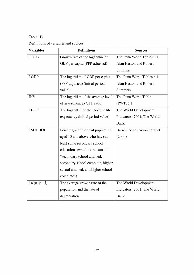
47
Table (1)
Definitions of variables and sources
Variables Definitions Sources
GDPG Growth rate of the logarithm of
GDP per capita (PPP-adjusted)
The Penn World Tables 6.1
Alan Heston and Robert
Summers
LGDP The logarithm of GDP per capita
(PPP-adjusted) (initial period
value)
The Penn World Tables 6.1
Alan Heston and Robert
Summers
INV The logarithm of the average level
of investment to GDP ratio
The Penn World Table
(PWT, 6.1)
LLIFE The logarithm of the index of life
expectancy (initial period value)
The World Development
Indicators, 2001, The World
Bank
LSCHOOL Percentage of the total population
aged 15 and above who have at
least some secondary school
education (which is the sum of
“ secondary school attained,
secondary school complete, higher
school attained, and higher school
complete” )
Barro-Lee education data set
(2000)
Ln (n+g+ )δ The average growth rate of the
population and the rate of
depreciation
The World Development
Indicators, 2001, The World
Bank

48
Table (2)
Descriptive statistics for all observations (1960-2000)
Variable Observations Mean Std. Dev. Min Max LGDP60 113 7.714 0.882 5.948 9.607 LGDP70 114 8.008 0.973 5.811 9.924 LGDP80 114 8.180 1.119 4.018 10.192 LGDP90 114 8.268 1.218 3.614 10.630 GDPG6069 113 2.835 2.268 -3.163 8.881 GDPG7079 113 2.252 2.776 -6.296 10.772 GDPG8089 114 0.909 2.554 -4.412 10.489 GDPG902000 114 1.356 2.541 -7.056 10.012 GDPG602000 113 1.688 2.058 -10.483 6.131 GDPG702000 114 1.319 2.447 14.987 6.105 GDPG802000 114 1.117 2.016 -4.655 6.257 LLIFE60 109 3.928 0.247 3.45 4.3 LLIFE70 109 4.006 0.218 3.54 4.31 LLIFE80 109 4.069 0.205 3.57 4.34 LLIFE90 111 4.128 0.194 3.56 4.37 LSHOOL60 90 2.533 1.179 -0.1053 4.5705 LSCHOOL70 92 2.844 1.154 0.0953 4.6643 LSCHOOL80 96 3.265 1.053 0.1823 5.0530 LSCHOOL90 98 3.548 0.960 0.8329 4.9530 LINV6069 114 2.7928 0.9410 0.001 4.011 LINV7079 112 2.9865 0.8272 0.177 4.438 LINV8089 114 2.8742 0.6780 0.815 4.369 LINV6099 112 2.6443 0.6633 0.706 3.888 LINV7099 112 2.6701 0.6461 0.771 4.01 LINV8099 114 2.6515 0.6389 1.068 4.018 LINV9099 114 2.7221 0.7355 0.707 4.103 Source: see table (1)
Table (3)
Annual growth rate of real GDP per capita
Region (group) 1960-69 70-79 80-89 90-2000 60-2000 70-2000 80-2000
All countries 2.83 2.25 0.90 1.35 1.68 1.31 1.11
OECD+SSA 2.73 1.66 0.69 0.72 1.13 0.74 0.65
OECD+ASIA 3.66 3.18 2.36 2.31 2.90 2.63 2.40
OECD+LA1 3.14 2.51 0.77 1.92 2.11 1.76 1.40
AFR+ASIA+LA 2.45 2.09 0.50 1.23 1.39 1.04 0.83
OECD 3.82 2.48 1.91 1.84 2.52 2.19 1.96
SSA 1.94 1.13 0.05 0.04 0.41 -0.07 -0.05
HIPCs2 1.50 0.56 -0.75 -0.45 -0.25 -0.80 -0.67
Source: own calculations based on PWT 6.1 1. LA = Latin Amrica. 2. Hevily indebted poor countries

49
Table (4)
Regression results for cross-sections of countries
Countries Period No. Obs. ββββa R2 t-valueb Probability
All 1960-2000 113 -0.06 0.026 1.75 0.08 1970-2000 113 -0.08 0.023 1.65 0.10 1980-2000 114 -0.12 0.100 3.57 0.00 1990-2000 114 -0.18 0.063 2.75 0.00 OECD 1960-2000 75 0.04 0.008 -0.91 0.36 and 1970-2000 75 -0.04 0.007 -0.22 0.29 Non-SSA 1980-2000 75 0.11 0.005 -0.59 0.59 1990-2000 75 0.07 0.024 -1.64 0.10 OECD 1960-2000 62 -0.08 0.059 2.45 0.00 and 1970-2000 63 -0.10 0.082 2.10 0.03 SSA 1980-2000 63 -0.14 0.252 4.71 0.00 1990-2000 63 -0.20 0.143 3.09 0.00 OECD 1960-2000 40 0.06 0.064 -1.61 0.11 and 1970-2000 41 0.07 0.070 -1.99 0.05 ASIA 1980-2000 41 0.09 0.125 -2.28 0.02 1990-2000 41 0.11 0.107 -2.11 0.04 OECD 1960-2000 42 -0.07 0.041 1.46 0.15 and 1970-2000 43 -0.07 0.034 1.29 0.20 Latin America 1980-2000 43 -0.02 0.143 2.73 0.00 1990-2000 43 0.21 0.021 -1.08 0.28 AFRICA, 1960-2000 89 -0.01 0.001 0.38 0.70 ASIA, 1970-2000 89 -0.03 0.002 0.46 0.64 and 1980-2000 89 -0.12 0.061 2.54 0.01 L.America 1990-2000 89 -0.21 0.070 2.61 0.01 OECD 1960-2000 23 0.10 0.631 -5.49 0.00 1970-2000 24 0.17 0.325 -3.08 0.00 1980-2000 24 0.15 0.149 -1.82 0.08 1990-2000 24 0.30 0.249 -2.58 0.01
Note: Heteroskedasticity has been corrected using the White direct method for correcting
heteroscedasticity, which is available in E-Views package. a. β has been computed from the OLS regression coefficient on initial GDP per capita using the
following formula: ( )
TbT+−= 1lnβ , where b is the coefficient on the initial GDP per capita and T is
the time period over which the growth rate is averaged. b.the t-values represent for the coefficient on the initial GDP per capita (LGDPI), which is “ b” , which has
not been reported here for space consumption reasons.

50
Table (5)
Variance of GDP per capita (σ- convergence)
Regions Years Variance ( 2σ ) Regions Years Variance ( 2σ ) GDP60 0.7788 GDP60 0.6345 GDP69 0.9117 GDP69 0.7093 GDP70 0.9480 OECD & GDP70 0.7227
All GDP79 1.0574 Non-SSA GDP79 0.7462 GDP80 1.2532 GDP80 0.7755 GDP89 1.4259 GDP89 0.8322 GDP90 1.4839 GDP90 0.8556 GDP2000 1.7045 GDP2000 0.8752 GDP60 1.1649 GDP60 0.3520 GDP69 1.3679 GDP69 0.4008 GDP70 1.4160 GDP70 0.4256 OECD&SSA GDP79 1.5798 SSA GDP79 0.4598 GDP80 1.9168 GDP80 0.7107 GDP89 2.2139 GDP89 0.8618 GDP90 2.3153 GDP90 0.9022 GDP2000 2.6796 GDP2000 1.1105 GDP60 0.9051 GDP60 0.4377 GDP69 0.9756 GDP69 0.5239 GDP70 0.9748 GDP70 0.5497
OECD and GDP79 0.9548 AFRICA, ASIA, GDP79 0.6565 ASIA GDP80 0.9887 and GDP80 0.8414 GDP89 0.9569 L. America (LA) GDP89 0.9557 GDP90 0.9816 GDP90 0.9945 GDP2000 0.9267 GDP2000 1.2208 GDP60 0.5102 GDP60 0.1502 GDP69 0.6282 GDP69 0.0824 GDP70 0.6265 GDP70 0.0725
OECD and GDP79 0.6398 OECD GDP79 0.0499 L. America GDP80 0.6734 GDP80 0.0614
GDP89 0.8465 GDP89 0.0540 GDP90 0.8865 GDP90 0.0702 GDP2000 0.8739 GDP2000 0.0532
Source: Own calculations using the PWT (6.1) data base

51
Conditional convergence
A. Results for cross-section regression for all Table (6)
Dependent variable is growth rate of log of real GDP per capita (1960-69)
Variable 1 2 3 4 CONSTANT 3.489
(1.32) 4.971*
(1.84) -6.534*
(-1.71) -4.884 (-1.14)
LGDP60 -0.429 (-1.18)
-0.569 (-1.56)
-0.647*
(-1.91) -0.670**
(-1.97) LINV6069 1.084***
(5.0) 0.994***
(4.56) 0.927***
(3.9) 0.903 (3.77)
LSCHL60 0.332 (1.37)
0.336 (1.42)
LLIFE60 3.219**
(2.39) 2.894**
(2.06) Log (n+g+δ ) -0.537***
(-2.57) -0.515**
(-2.50) -0.393*
(-1.84) -0.398*
(-1.86) HIPCs -1.001*
(-1.97) -0.433
(-0.85) No. of Observation 88 88 107 107 R2 0.37 0.40 0.33 0.34
For all regression results , the asterisks *, **, and *** indicate significance leveles at 10%, 5% and 1% , respectively. Table (7)
Dependent variable is growth rate of log of real GDP per capita (1970-79)
Variable 1 2 3 4 CONSTANT 4.725
(1.35) 8.105**
(2.34) -20.018***
(-3.57) -16.261***
(-2.72) LGDP70 -1.301***
(-2.77) -1.55***
(-3.44) -1.374***
(-3.89) -1.414***
(-4.03) LINV7079 1.901***
(5.42) 1.623***
(4.74) 1.555***
(4.67) 1.448***
(4.31) LSCHL70 0.824**
(2.46) 0.792**
(2.5)
LLIFE70 6.918***
(3.93) 6.192***
(3.45) Log (n+g+δ ) 0.053
(0.17) 0.038 (0.13)
0.392*
(1.73) 0.414*
(1.84) HIPCs -2.144
(0.13) -0.998*
(-1.68) No. of Observation 88 88 105 105 R2 0.33 0.41 0.44 0.46

52
Table (8)
Dependent variable is growth rate of log of real GDP per capita (1980-89)
Variable 1 2 3 4 CONSTANT 4.339
(1.52) 6.625**
(2.14) -0.871 (-0.14)
3.522 (0.53)
LGDP80 -0.972**
(-2.51) -1.097***
(-2.82) -0.980***
(-3.23) -1.128***
(-3.66) LINV8089 1.956***
(4.65) 1.705***
(3.88) 1.958***
(4.57) 1.735***
(3.97) LSCHL80 0.175
(0.56) 0.107 (0.35)
LLIFE80 1.44 (0.77)
0.915 (0.49)
Log (n+g+δ ) -0.843***
(-3.01) -0.863***
(-3.11) -0.857***
(-3.38) -0.90***
(-3.58) HIPCs -1.149*
(-1.78) -1.218**
(-2.03) No. of Observation 95 95 108 108 R2 0.30 0.32 0.37 0.40 Table (9)
Dependent variable is growth rate of log of real GDP per capita (1990-2000)
Variable 1 2 3 4 CONSTANT 4.706
(1.58) 8.587***
(2.84) -13.762*
(-1.8) -4.593 (-0.57)
LGDP90 -0.908**
(-2.23) -1.131***
(-2.9) -0.980***
(-2.69) -1.061***
(-3.0) LINV902000 1.273***
(3.12) 0.987**
(2.51) 1.215***
(2.87) 0.973**
(2.32) LSCHL90 0.683*
(1.88) 0.448 (1.28)
LLIFE90 5.071 (2.26)
3.285 (1.45)
Log (n+g+δ ) -0.876 (-2.57)
-0.794**
(-2.46) -0.547*
(-1.71) -0.531*
(-1.71) HIPCs -2.304***
(-3.48) -1.897***
(-2.78) No. of Observation 97 97 110 110 R2 0.24 0.33 0.23 0.29

53
Table (10)
Dependent variable is growth rate of log of real GDP per capita (1960-2000)
Variable 1 2 3 4 CONSTANT 7.642***
(3.91) 10.07***
(5.51) -10.702***
(-2.75) -6.779*
(-1.81) LGDP60 -1.221***
(-4.85) -1.386***
(-6.09) -1.503***
(-5.87) -1.621***
(-6.77) LINV6099 1.546***
(6.96) 1.162***
(5.39) 1.23
(4.28) 0.845***
(2.99) LSCHL60 0.441***
(2.73) 0.490***
(3.38)
LLIFE60 5.473***
(4.56) 5.056***
(4.51) Log (n+g+δ ) -0.711***
(-4.04) -0.676***
(-4.29) -0.376*
(-1.64) -0.356*
(-1.68) HIPCs -1.582***
(-4.62) -1.563***
(-4.08) No. of Observation 86 86 105 105 R2 0.55 0.64 0.54 0.60 Table (11)
Dependent variable is growth rate of log of real GDP per capita (1970-2000)
Variable 1 2 3 4 CONSTANT 9.409**
(4.18) 11.928***
(5.63) -16.421***
(-2.78) -11.256*
(-1.91) LGDP70 -1.626***
(-5.57) -1.781***
(-6.57) -1.806***
(-6.25) -1.889***
(-6.79) LINV7099 1.876***
(6.85) 1.413***
(5.24) 1.614***
(4.25) 1.24***
(3.28) LSCHL70 0.652***
(3.2) 0.655***
(3.55)
LLIFE70 7.190***
(4.25) 6.414***
(3.9) Log (n+g+δ ) -0.804***
(-3.8) -0.768***
(-4.0) -0.469*
(-1.64) -0.469*
(-1.71) HIPCs -1.761***
(-4.38) -1.564***
(-3.13) No. of Observation 89 89 106 106 R2 0.51 0.60 0.51 0.56

54
Table (12)
Dependent variable is growth rate of log of real GDP per capita (1980-2000)
Variable 1 2 3 4 CONSTANT 6.644***
(3.06) 9.759***
(4.47) -1.746 (-0.35)
2.814 (0.58)
LGDP80 -1.153***
(-4.06) -1.328***
(-4.94) -0.748***
(-3.25) -0.907***
(-4.09) LINV8099 1.781***
(5.44) 1.401***
(4.37) 1.679***
(4.74) 1.293***
(3.7) LSCHL80 0.374
(1.60) 0.287 (1.31)
LLIFE80 1.485 (1.04)
1.032 (0.76)
Log (n+g+δ ) -1.00***
(-4.4) -0.990***
(-4.65) -0.784***
(-3.51) -0.772***
(-3.66) HIPCs -1.729***
(-3.83) -1.618***
(-3.71) No. of Observation 95 95 108 108 R2 0.43 0.51 0.43 0.50
B. Regression results for panel data (decade averages (1960-2000) -All Table (13)
Descriptive statistics for panel data (1960-2000)-All
Variable No. of Obs. Mean Std.Dev. Min Max GDPG 454 1.8354 2.6428 -7.0562 10.7724 LGDPI 455 1.8354 1.074 3.6144 10.6306 LLIFE 438 4.0336 0.2291 3.45 4.37 SCHOOL 358 1.1944 1.1302 0.001 5.742 INV 359 3.3196 0.3956 1.98 4.32 Ln(n+g+δ ) 452 2.0253 1.061 -3.634 5.9592

55
Table (14)
Cross-section pooled time series (1960-2000)-All
Variable 1 2 3 4 5 6 Constant 5.157***
(3.47) 8.176***
(5.37) 7.429***
(5.06) -2.321 (-0.87)
2.167 (0.77)
-5.529*
(-1.79) LGDPI -1.039***
(-5.04) -1.247***
(-6.19) -1.212***
(-6.3) -0.912***
(-5.24) -1.028***
(-5.97) -1.013***
(-6.17) LINV 1.907***
(10.5) 1.594***
(8.72) 1.409***
(7.72) 1.878***
(10.52) 1.686***
(9.37) 1.415***
(7.73) LSCHL 0.272*
(1.77) 0.253*
(1.71) 0.482***
(3.2)
LLIFE 1.678**
(2.02) 1.02
(1.23) 2.95***
(3.36) LPOPG -0.592***
(-4.13) -0.574***
(-4.18) -0.574***
(-4.37) -0.328**
(-2.51) -0.325***
(-2.54) -0.257***
(-2.10) HIPCs -1.825***
(-5.69) -1.621***
(-5.25). -1.385***
(-4.46) -1.101***
(-3.68) 1960s 1.164***
(3.66) 1.444*
(4.48) 1970s 0.609**
(1.96) 0.552*
(1.79) 1980s -0.622**
(-2.18) -0.572**
(-1.99) No. Obser. 372 372 372 430 430 430 R2 0.28 0.34 0.40 0.28 0.31 0.38

56
Table (15)
Regression results for panel data (1960-2000)
Random Effects Model Fixed Effects Model Variable 1 2 3 4 5 6 7 8 Const. 6.372***
(3.64) 9.329***
(5.32) 8.065***
(4.74) -5.301 (-1.61)
19.03***
(6.28) 19.03***
(6.28) 16.701***
(4.56) 9.487 (1.17)
LGDPI -1.246***
(-5.34) -1.427***
(-6.36) -1.337***
(-6.21) -1.063***
(-6.12) -2.662***
(-7.57) -2.662*** (-7,57)
-2.416***
(-6.00) -1.738***
(-5.69) LINV 2.089***
(10.31) 1.743***
(8.68) 1.542***
(7.58) 1.492***
(7.71) 1.537***
(5.09) 1.537***
(5.09) 1.701***
(5.56) 1.906***
(6.4) LSCHL 0.226
(1.38) 0.209 (1.34)
0.487***
(2.99) 0.187
(0.97) 0.187 (0.97)
0.232 (0.99)
LLIFE 2.935***
(3.17) 0.279
(0.16 Log (n+g+δ )
-0.563***
(-3.31) -0.547***
(-3.45) -0.551***
(-3.62) -0.236*
(-1.84) -0.226 (-0.87)
-0.226 (-0.87)
-0.22 (-0.84)
-0.046 (-0.25)
HIPCs -2.053***
(-5.17) -1.717***
(-4.44) -1.123***
(-3.34)
1960s 1.068***
(3.54) 1.397***
(4.42) -0.062
(-0.14) 0.386 (0.79)
1970s 0.521*
(1.8) 0.504*
(1.69) -0.203
(-0.57) -0.159 (-0.43)
1980s -0.666***
(-4.44) -0.593**
(-2.16) -0.956***
(-3.57) -0.903***
(-3.12) No. Obser. 372 372 372 430 372 372 372 430 R2 0.20 0.23 0.30 0.29 0.29 0.29 0.33 0.31 Prob(Chi2)1 0.000 0.000 0.055 0.031 1. The hausman test for column 3 and 4 accepts the Ho, so I opt for the random effects model, while column 1 and 2 rejects it, therefore I opt for the fixed effects model

57
C. Cross-section results for developing countries’ convergence
Table (16)
Descriptive statistics for developing countries (1960-2000)
Variable Observations Mean Std. Dev. Min Max LGDP60 91 7.421 0.689 5.948 9.016 LGDP70 91 7.678 0.772 5.811 9.333 LGDP80 91 7.833 0.950 4.018 9.727 LGDP90 91 7.898 1.038 3.614 9.944 GDPG6069 91 2.576 2.296 -3.163 8.606 GDPG7079 91 2.236 3.021 -6.296 10.772 GDPG8089 91 0.728 2.769 -4.412 10.489 GDPG602000 91 1.308 2.735 -7.056 10.129 GDPG702000 91 1.170 2.647 -14.978 6.105 GDPG802000 91 0.976 2.138 -4.655 6.105 GDPG902000 91 1.308 2.735 -7.056 10.012 LSCHL60 68 2.1544 1.001 -0.1053 4.0377 LSCHL70 70 2.4782 1.0309 0.0953 4.5261 LSCHL80 74 2.9634 0.9643 0.1823 4.5261 LSCHL90 76 2.9634 0.9643 0.1823 4.8434 LLIFE60 86 3.851 0.211 3.45 4.3 LLIFE70 86 3.944 0.195 3.54 4.31 LLIFE80 86 4.014 0.188 3.57 4.33 LLIFE90 88 4.081 0.185 3.56 4.35 INV6069 91 2.607 0.8814 0.482 3.935 INV7079 88 2.8049 0.8351 0.177 4.438 INV8089 90 2.709 0.661 0.815 4.369 INV6099 88 2.4821 0.6426 0.706 3.888 INV7099 88 2.5059 0.6241 0.771 4.01 INV8099 90 2.491 0.6095 1.068 4.018 INV902000 90 2.5436 0.715 0.707 4.103

58
Table (17)
Cross-section results for developing countries (1960-2000)
Variable 1 2 3 4 CONSTANT 7.266***
(2.99) 10.347***
(4.51) -11.206**
(-2.46) -6.548 (-1.48)
LGDP60 -1.147***
(-3.54) -1.424***
(-4.8) -1.489***
(-4.69) -1.726***
(-5.72) LINV6099 1.621***
(6.18) 1.190***
(4.63) 1.303***
(4.01) 0.881***
(2.72) LSCHL60 0.446**
(2.09) 0.538***
(2.81)
LLIFE60 5.612***
(4.15) 5.193***
(4.11) Log (n+g+δ ) -0.846
(-3.6) -0.741***
(-3.52) -0.485*
(-1.64) -0.378 (-1.37)
HIPCs -1.551***
(-4.04) -1.578***
(-3.63) No. of Observation 64 64 82 82 R2 0.55 0.65 0.53 0.60 Table (18)
Cross-section results for developing countries(1970-2000)
Variable 1 2 3 4 CONSTANT 8.991***
(3.34) 12.155***
(4.71) -16.023**
(-2.37) -10.73 (-1.59)
LGDP70 -1.522***
(-4.24) -1.761***
(-5.31) -1.837***
(-5.17) -2.032***
(-5.84) LINV7099 1.985***
(6.34) 1.491***
(4.77) 1.726***
(4.09) 1.297***
(2.99) LSCHL70 0.606**
(2.41) 1.491***
(2.84)
LLIFE70 7.172***
(3.76) 6.552***
(3.55) Log (n+g+δ ) -1.01***
(-3.75) -0.906***
(-3.69) -0.609*
(-1.67) -0.518 (-1.47)
HIPCs -1.691***
(-3.77) -1.581***
(-2.78) No. of Observation 66 66 82 82 R2 0.55 0.64 0.53 0.58

59
Table (19)
Cross-section results for (1980-2000)
Variable 1 2 3 4 CONSTANT 6.475**
(2.58) 9.965***
(3.84) -1.761 (-0.33)
2.466 (0.46)
LGDP80 -1.067***
(-3.18) -1.318***
(-4.06) -0.677**
(-2.56) -0.884***
(-3.37) LINV8099 1.964***
(5.26) 1.574***
(4.24) 1.802***
(4.57) 1.428***
(3.59) LSCHL80 0.299
(1.05) 0.225 (0.83)
LLIFE80 1.468 (0.95)
1.122 (0.76)
Log (n+g+δ ) -1.294***
(-4.49) -1.219***
(-4.49) -1.073***
(-3.93) -0.995***
(-3.79) HIPCs -1.61***
(-3.18) -1.439***
(-2.96) No. of Observation 72 72 84 84 R2 0.48 0.55 0.49 0.52 Table (20)
Cross-section results for developing countries (1990-2000)
Variable 1 2 3 4 CONSTANT 4.473
(1.27) 8.720**
(2.36) -12.716 (-1.53)
-4.881 (-0.55)
LGDP90 -0.744 (-1.5)
-1.073**
(-2.19) -0.917***
(-2.09) -1.082**
(-2.49) LINV902000 1.381***
(3.08) 1.138**
(2.6) 1.36***
(2.91) 1.123**
(2.4) LSCHL90 0.643
(1.45) 0.433 (1.0)
LLIFE90 4.82**
(1.97) 3.457 (1.4)
Log (n+g+δ ) -1.349***
(-3.27) -1.209***
(-3.04) -0.887**
(-2.25) -0.813**
(-2.11) HIPCs -2.024***
(-2.74) -1.683**
(-2.22) No. of Observation 74 74 86 86 R2 0.33 0.40 0.29 0.33

60
Table (21)
Cross-section results for developing countries (1960-69)
Variable 1 2 3 4 CONSTANT 2.561
(0.8) 4.135 (1.26)
-7.277 (-1.52)
-5.895 (-0.56)
LGDP60 -0.368 (-0.80)
-0.526 (-1.14)
-0.382 (-0.95)
-0.417 (-1.02)
LINV6069 1.147***
(4.23) 1.047***
(3.82) 1.027***
(3.53) 1.01***
(3.42) LSCHL60 0.363
(1.23) 0.373 (1.29)
LLIFE60 2.875*
(1.89) 2.618*
(1.64) Log (n+g+δ ) -0.459*
(-1.76) -0.425*
(-1.65) -0.438*
(-1.66) -0.432 (-1.63)
HIPCs -0.895*
(-1.69) -0.306
(-0.56) No. of Observation 66 66 84 84 R2 0.33 0.36 0.31 0.31 Table (22)
Cross-section results for developing countries (1970-79)
Variable 1 2 3 4 CONSTANT 3.828
(0.89) 7.783*
(1.82) -21.981***
(-3.4) -17.684**
(-2.51) LGDP70 -1.182**
(-1.98) -1.533**
(-2.65) -1.331***
(-3.09) -1.432***
(-3.31) LINV7079 1.92***
(4.76) 1.638**
(2.29) 1.58***
(4.28) 1.469***
(3.92) LSCHL70 0.924**
(2.21) 0.908**
(2.29)
LLIFE70 7.336***
(3.77) 6.573***
(3.28) Log (n+g+δ ) -0.037
(-0.09) 0.001 (0.01)
0.386 (1.47)
0.429 (1.64)
HIPCs -2.098***
(-2.88) -0.978
(-1.47) No. of Observation 66 66 82 82 R2 0.40 0.44 0.47 0.48

61
Table (23)
Cross-section results for developing countries (1980-89)
Variable 1 2 3 4 CONSTANT 4.596
(1.32) 7.403*
(1.91) -1.249 (-0.17)
3.013 (0.39)
LGDP80 -0.998**
(-2.06) -1.187**
(-2.4) -0.891**
(-2.43) -1.08***
(-2.83) LINV8089 2.03***
(4.06) 1.743***
(3.31) 1.986***
(4.03) 1.765***
(3.49) LSCHL80 0.147
(0.36) 0.073 (0.18)
LLIFE80 1.463 (0.68)
1.01 (0.47)
Log (n+g+δ ) -0.914**
(-2.42) -0.892**
(-2.39) -1.025***
(-3.15) -1.024***
(-3.18) HIPCs -1.214
(-1.59) -1.134
(-1.63) No. of Observation 72 72 84 84 R2 0.26 0.28 0.35 0.38

62
D. Panel Regression for developing countries (1960-2000) Table (24)
Descriptive Statistics for Developing countries’ Panel (1960-2000)
Variable Observation Mean Std. Dev. Min Max LGDPG 360 1.650 2.836 -7.056 10.77 LGDPI 360 7.67 0.859 3.614 9.94 LLIFE 342 3.961 0.207 3.45 4.35 LSCHL 284 2.743 1.062 -0.105 4.84 LINV 358 2.665 0.780 0.177 4.43 Ln(n+g+ )δ 352 2.364 0.902 -3.63 5.96
Table (25)
Cross-section pooled time series results for developing countries (1960-2000)10
Variable 1 2 3 4 CONSTANT 3.121*
(1.66) 7.013***
(3.61) 6.259***
(3.37) -7.506**
(-2.05) LGDP -0.640**
(-2.44) -0.999***
(-3.84) -1.014***
(-4.08) -0.952***
(-4.68) LINV 1.752***
(8.6) 1.466***
(7.24) 1.374***
(6.98) 1.387***
(6.97) LSCHL 0.109
(0.59) 0.121 (0.68)
0.424**
(2.27)
LLIFE 3.378***
(3.34) Log (n+g+δ ) -0.645***
(-3.38) -0.585***
(-3.2) -0.616***
(-3.52) -0.342**
(-2.28) HIPCs -1.839***
(-5.17) -1.574***
(-4.59) -0.988***
(-2.93) 1960s 1.223***
(3.0) 1.652***
(4.06) 1970s 0.852**
(2.16) 0.786**
(2.07) 1980s -0.773**
(-2.15) -0.626*
(-1.76) No. of Observation 278 278 278 336 R2 0.25 0.32 0.39 0.37 10. dependent variable is growth rate of log GDP per capita

63
Table (26)
Panel regression results for developing countries (1960-2000)
Random Effects Model Fixed Effects Model Variable 1 2 3 4 5 6 7 8 Const. 4.88**
(2.24) 8.484***
(3.88) 7.279***
(3.46) -7.437**
(-1.95) 21.071***
(5.58) 21.071***
(5.58) 17.31***
(4.13) 4.897 (0.51)
LGDPI -0.904***
(-3.02) -1.203***
(-4.16) -1.181***
(-4.26) -0.992***
(-4.73) -2.884***
(-6.02) -2.884***
(-6.02) -2.498***
(-5.0) -1.698***
(-4.84) LINV 1.838***
(8.05) 1.528***
(6.9) 1.442***
(6.65) 1.412***
(6.88) 1.379***
(4.05) 1.379 (4.05)
1.505***
(4.43) 1.714***
(5.2) LSCHL 0.079
(0.41) 0.09
(0.49) 0.454**
(2.26) 0.117
(0.50) 0.117 (0.50)
0.293 (0.97)
LLIFE 3.411***
(3.26) 1.333
(0.61) Log (n+g+δ )
-0.603***
(-2.77) -0.555***
(-2.73) -0.596***
(-3.04) -0.318**
(-2.07) -0.458 (-1.45)
-0.458 (-1.45)
-0.408 (-1.28)
-0.059 (-0.28)
HIPCs -2.053***
(-4.88) -1.683***
(-4.09) -1.013***
(-2.83)
1960s 1.165***
(2.94) 1.632***
(4.04) 0.171
(0.30) 0.731 (1.16)
1970s 0.799**
(2.12) 0.767**
(2.05) 0.161
(0.35) 0.177 (0.38)
1980s -0.797**
(-2.39) -0.637*
(-1.83) -1.033***
(-2.95) -0.932***
(-2.53) No. Obser. 278 278 278 336 278 278 278 336 R2 0.13 0.49 0.24 0.25 0.23 0.23 0.29 0.28 Prob(Chi2)1 0.000 0.000 0.17 0.044 1.The Prob (Chi2) in columns 1 and 2 indicate that one the Hausman test is in favor of the fixed effects model while in colums 3 and 4, the Hausman test indicate that the random effects model should be chosen.

64
E. Panel Regression for HIPCs (1960-2000) Table (27)
Descriptive statistics for HIPCs (1960-2000) four decades panel
Variable Observation Mean Std.Dev. Min Max GDPG 116 0.2148 2.6351 -7.0562 6.6288 Log (GDPI) 116 7.034 0.6896 3.144 8.2961 Log (INV) 90 3.085 0.4621 1.98 3.87 LLIFEI 112 3.8085 0.1527 3.45 4.2 POPG 116 2.637 0.6836 -0.46 4.25 Table (28)
Cross-section pooled time series results (1960-2000) decade averages-HIPCs alone
Variable 1 2 3 Constant 2.188
(1.42) 12.551*
(1.92) -1.614 (-0.23)
GDPI -1.67***
(-3.46) -1.375***
(-2.61) -1.789***
(-3.56) INV 2.109***
(4.03) 2.272***
(4.25) 2.369***
(4.73) LLIFEI -2.581
(-1.35) 1.601 (0.78)
POPG 0.226 (0.61)
0.208 (0.56)
0.148 (0.43)
Dummy for 1960s 2.636***
(3.7) Dummy for 1970s 1.282**
(1.98) Dummy for 1980s 0.078
(0.13) No. Observations 90 90 90 R2 0.21 0.22 0.37

65
Table (29)
Regression results using a panel data (1960-2000) decade averages-HIPCs alone
Random Effects Model Fixed Effects Model Variable 1 2 3 4 CONST 12.552*
(1.92) -1.614 (-0.23)
63.85***
(6.23) 56.542**
(2.43) LGDPI -1.375***
(-2.61) -1.789***
(-3.56) -5.441***
(-5.27) -5.297***
(-4.84) INV 2.272***
(4.25) 2.369***
(4.73) 1.334*
(1.89) 1.239*
(1.72) LLIFE -2.581
(-1.35) 1.601 (0.78)
-8.022***
(-3.39) -6.385 (-1.19)
POPG 0.208 (0.56)
0.148 (0.44)
0.68 (1.29)
0.673 (1.21)
Dummy for 1960s 2.636***
(3.7) 0.296
(0.22) Dummy for 1970s 1.282**
(1.98) 0.228
(0.26) Dummy for 1980s 0.078
(0.13) -0.276
(-0.45) No. observations 90 90 90 90 R2 0.23 0.37 0.49 0.50 Prob (Chi2)1 0.000 0.04 1. Prob (Chi2) = 0.04 is a Hausman test that indicates that the random effects model in column 1 is a more appropriate model to use for this regression, while column 2 indicates the other way around.

66
Table (30)
List of countries included in the regression
Angola Cape Verde Guyana Mozambique Senegal
Argentina Costa Rica Hong Kong, China Mauritania Singapore
Australia Ecuador Honduras Mauritius Sierra Leone Austria Egypt, Arab Rep. Haiti Malawi El Salvador Burundi Denmark Indonesia Malaysia Sweden Belgium Cyprus India Namibia Seychelles
Benin Dominican Republic Ireland Niger
Syrian Arab Republic
Burkina Faso Algeria Iran, Islamic Rep. Nigeria Chad Bangladesh Spain Iceland Nicaragua Togo Bolivia Ethiopia Israel Netherlands Thailand Brazil Finland Italy Norway Trinidad and Tobago Barbados Fiji Jamaica Nepal Tunisia Botswana France Jordan New Zealand Turkey Central African Republic Germany Japan Pakistan Tanzania Canada Gabon Kenya Panama Uganda Switzerland United Kingdom Korea, Rep. Peru Uruguay Chile Ghana Sri Lanka Philippines United States China Guinea Lesotho Papua New Guinea Venezuela, RB Cote d'Ivoire Gambia, The Luxembourg Portugal South Africa Cameroon Guinea-Bissau Morocco Paraguay Congo, Dem. Rep. Congo, Rep. Equatorial Guinea Madagascar Romania Zambia Colombia Greece Mexico Rwanda Zimbabwe Comoros Guatemala Mali

67
Unconditional convergence (graphic representation) Graph (A1)
Graph (A2)

68
Graph (A3)
Graph(A4)

69
Graph (A5)
Graph (A6)

70
Graph (A7)
Graph (A8)

71
Graph (A9)
Graph (A10)

72
Graph (A11)
Graph (A12)

73
Graph (A13)
Graph (A14)

74
Graph (A15)

II. An Empirical Exploration into the
Determinants of External Indebtedness

76
Abstract
The causes of the external indebtedness of developing countries and their subsequent failure to
meet contractual debt obligations have generated the heated debates both in the academic circles,
policy makers, and the broader international community since the outset of the debt crisis in
1982. While poverty and external factors seem to be the most profound factors behind the
external indebtedness of poor nations, there is still an ongoing debate on the determinants of the
demand for overseas borrowing by developing countries.
This chapter contributes to this debate by empirically investigating the causes of external
indebtedness by developing countries in the 1980s and 1990s. First, I empirically examine the
robustness of a recent study, which is based on the hypothesis that indebted countries have a
greater tendency to exercise bad policies. Second, moving to a broader approach and using annual
cross-section, fixed effects and random effects models and cross-section pooled time series
strategies, this paper shows that poverty (the savings gap), income instability, and external factors
that include debt service payments to be the main causes of overseas borrowing by developing
countries in the 1980s and 1990s.
As far as the empirical strategy is concerned, the application of a panel data approach seems to be
highly preferred, as it allows us control for time-specific events that are linked to overseas
borrowing, particularly given the rapid changes in the global macroeconomic environment in the
past years. Moreover, this strategy helps to produce a more robust explanation by allowing to
incorporate country-specific factors as developing countries themselves are heterogeneous in
terms of their colonial heritages, geopolitical and strategic significance, and creditworthiness, all
affecting the level of indebtedness and the potential bargaining power to manage the subsequent
debt crisis.

77
1. Introduction “ International debt has become the defining feature of the contemporary world economy” , (Eatwell and Taylor, 2000, in: Dymski, 2002, p. 244) The problem of developing countries’ external debt is believed to be one of the major
challenges of the new millennium The debate has been further intensified thanks to the
involvement of not only the traditional international financial institutions, but also
independent analysts, and non-governmental organizations (NGOs). Though it is
generally believed that external debt helps countries that are suffering from capital
deficiency to achieve accelerated economic growth, once this financial gap becomes
unmanageable, the past accumulated external debt is likely to provoke further external
borrowing, creating a vicious circle problem. This obviously creates a gloomy picture on
future growth prospects and reduces the likelihood of developing countries to meet their
debt-service obligations, which is exactly the current experience of the poorest nations of
the world, earning the new name “ heavily indebted poor countries” (HIPCs).
It is particularly crucial given the factors behind this huge debt build up. Although
poverty (the savings gap) seems to be the natural reason behind overseas borrowing, there
are additional, mainly exogenous, factors that drove most developing nations into a
chronic external debt crisis situation. The most frequently cited determinants of overseas
borrowing in the 1970s and 1980s are the two-oil price shocks of the early and late
1970s, and the subsequent recession in major industrialized countries, the change in the
global economic policy and the deterioration in developing countries terms of trade are
just to mention a few. On the supply side, the generous and irresponsible lending policies
of private commercial banks in industrialized countries that are linked to the recycling of
the “ Petrodollars” are another widely acknowledged root causes behind developing
countries debt accumulation. What is even worse in this context is that as private
commercial banks were fast to discharge loans to developing countries in the 1970s, they
were even faster to cut lending when the first sign of the debt crisis came into play

78
following Mexico’ s official announcement in August 1982 that it was no longer able and
willing to meet its contractual debt obligation. 15
It should, however, be added that irresponsible and corrupt governments (sometimes
unelected ones) in developing countries themselves are the key players of the debt build
up. Such leaders across the developing world, like Mobutu of Zaire, have been accused of
shamelessly squandering their nations’ scarce resources for luxurious activities rather
than investing them to improve the lives of these desperately poor nations. The joint
effects of all these and other factors led most indebted countries to experience multiple
debt crisis, which ultimately forced them to undertake frequent rescheduling and beg for
debt reduction and relief.
The objective of this chapter is to add to the current empirical literature on the
determinants of overseas borrowing by developing countries in 1980s and 1990s. To
answer this question, the remainder of the paper is divided into three parts. Part 2
presents the general theoretical discussion on the evolution of the debt crisis, including
the magnitude and structure of developing countries external debt with emphasis on
HIPCs. In section 2.2., I investigate the robustness of Easterly’ s (2002) study on the
determinants of HIPCs external borrowing using a cross-section, and cross-section
pooled times series, fewer countries and slightly different time period. In section 2.3,
using annual cross-section, panel data and cross-section pooled time series approachs; I
present a further empirical investigation into the causes of indebtedness across HIPCs and
non-HIPCs developing countries during the 1980s and 1990s. Finally, part three
summarizes the highlights of this study and its policy implications.
15 The abnormal nature of the external debt problem of developing countries in the 1970s and 1980s was best expressed by the popular joke of the 1930s, which characterizes private credit as ” an umbrella that a person is allowed to borrow as long as the weather is fine, but which he has to return the moment it starts raining” Anonymous (in: Wayne, 1993).

79
2. Why indebted countries got indebted in the first place? A theoretical explanation
External borrowing is not a new phenomenon at all. Most of today’ s industrialized
countries had been net borrowers in their path to economic development. But the reasons
for being indebted might differ from country to country and time to time. This part
mainly discusses the reasons behind developing countries indebtedness in the 1980s and
1990s. The arguments for overseas borrowing and lending are numerous. Though as is
well known, there is a lender to every borrower, I will rather focus my analysis on the
indebted countries, hence the demand side of external indebtedness. The supply side will
only be marginally discussed when relevant. The causes of external indebtedness might
be classified into four categories: poverty-driven indebtedness, the foreign exchange gap,
the return argument, and the contribution of external factors, are just to mention the major
factors behind overseas borrowing.
A. The savings gap as a driving force behind external indebtedness
There is a widespread consensus among growth economists that poverty plays an
enormous role in driving countries into serious external indebtedness. In this context,
from the view point of debtors, the economic justification to borrow overseas is
associated with the rising gap between national savings and domestic investment.16 That
is, at the expense of running a current account imbalance, a country may manage to
obtain resources to invest even if its domestic savings levels are low. Several studies
associate the major cause of external indebtedness to the poverty-vicious circle type of
argument. For example, Singer (1990, in: Healey (1995)), argues that the external
imbalance is caused by the vicious circle of poverty: poor people are poor because they
are undernourished or illiterate, and they are undernourished and illiterate because they
are poor. In the same token, poor countries are poor because they have low savings and
investment and they have low savings and investment because they are poor.
16 For the formal treatment of the savings gap and the foreign exchange gap (the two-gap model), see Basu (2000).

80
Similarly, Root (1990) argues that the major development obstacle of developing
countries is the vicious circles of the saving-investment gap: productivity is low because
investment is low, investment is low because savings are low, saving are low because
income is low, income is low because productivity is low; thus, in a very real sense,
according to Root (1990), the poor nations are poor because they are poor. The savings
gap, therefore, reflects the inability of poor countries to save sufficient amount of
resources to finance the desired level of investment necessary for self-sustained growth.
Overseas borrowing is bound to fill this gap by generating resources that domestic savers
are unable or unwilling to sacrifice.17 With the elapse of time, growth in income should
boost domestic savings, eventually generating a surplus over investment which can be
used to repay the accumulated past borrowing. Furthermore, the absence of developed
(malfunctioning) financial system to mediate savings and investment in developing
countries makes the situation for savers difficult to place their funds directly into
investment opportunities leading to insufficient domestic savings available to provide the
finance for domestic investment (Gybson, 1996, among others). From this standpoint, it
is possible to argue that the deficit in poor countries is simply a development deficit that
is inevitable if countries are to achieve long-term positive economic growth. Such a
deficit, however, is not without cost as it increases foreign debt, which must be serviced
and repaid in the future. Pereira and Rosser (1996) also take this same line, where they
strongly link the external indebtedness of developing countries to their level of poverty.18
Table (1.1) below indicates that HIPCs are substantially lagging behind non-HIPCs
counterparts in income per capita level, gross domestic savings and investment, literacy
rates and life expectancy. In contrast, they send out more resources abroad in the form of
debt service payments.
17 Many believe that under the circumstances of low level of savings, overseas borrowing by the public sector may help the private investment via the public investment and avoids possible crowding out effect of the private investment through domestic borrowing. This may also feed the economy with additional foreign exchange to finance past accumulated debt and imports (Serieux, 2001). 18 Their analysis is based on the 1990 UN Chronicle that presents the following statistical evidence on poverty across the world (Pereira and Rosser, 1996, pp. 46): 1 billion people live in absolute poverty, 100 million persons are completely homeless, 800 million go hungry everyday, 1.75 billion people are without access to safe drinking water, and 1.5 billion are without access to primary education, an alarming figure that demonstrates the severity of poverty across developing countries, many of which are members of HIPCs.

81
Table (1.1)
Some economic and social indicators for HIPCs and Non-HIPCs (1980-98)
Heavily indebted poor countries
(HIPC) Low & middle income
Economic and social indicators 1980-89 1990-98 1980-89 1990-98
GDP per capita (constant 1995 US$)a 310.69 338.10 1158.65 1341.01
Gross Domestic Investment (% of GDP) 17.82 19.25 27.82 29.28
Gross Domestic Savings (% of GDP) 11.01 12.16 27.99 28.70
Total Debt Service (% of exports) 24.41 20.61 22.52 18.90
Illiteracy rate, adult total b 53 44 38 31
Life expectancy at birth, total (years) c 50 52 60 63
a. the 1980-89 average is only 1984-89
b. this is data for 1980 and 1990
c. this is data for 1980 and 1990 Source: own calculations based on data from the World Bank, World Development Indicator, 2001 (CD-ROM)
The poverty driven indebtedness is particularly alarming to heavily indebted poor
countries (HIPCs). As Serieux (2001, pp.307) rightly puts it, “ heavily indebted” and
“ poor” clearly spells out the combined attributes that HIPCs apart from other developing
countries and make them a focus of concern for northern governments, international
public agencies, and international civil-society organizations” . All the gap models argue
in this direction.19 Classens, et al (1997) also indicates that HIPCs situation differ from
other middle-income debtors in several respects that include the poor income level and
poor economic reform in this group (pp. 233). IMF in its recent study acknowledges that
“ the increase in many low-income countries’ debts, beginning in the 1970s and peaking
19 For a further discussion, see Agenor and Montiel (1996), Taylor (1994), and Bacha (1990), among others. In this context many argue that overseas borrowing may be beneficial to generate higher economic growth if an increase in investment contributes to higher growth, which generates additional foreign exchange to finance past accumulated debt. In this context Healey (1995) among others, argue that foreign capital would be translated into growth if the saving and foreign-exchange gaps can in due course be reversed, and the funds are invested in projects that generate higher rate of returns compared to the cost of borrowing, hence the market interest rate. Similarly, others, for example Easterly (1999) argue that if aid is viewed as a permanent income by a developing country government, the recipient government is highly likely to spend these resources on boosting consumption rather than investment, making aid meaningless in terms of boosting growth. The endogenous growth theory is also in this line. The central argument is that if aid is transferred as a lump sum, it would have no impact on investment.

82
in the 1980s, was accompanied by disappointing performance in their struggle against
poverty” (IMF, 2003, pp. 6).20
B. The foreign-exchange constraint
Another equally important justification behind the overseas borrowing of developing
countries is that of the foreign exchange gap. Because even assuming that there were no
capital deficiency and no savings gap that serve as a constraint to economic development,
the growth rate of developing countries may still be hindered by a foreign exchange gap.
This seems to suggest that domestic savings in developing countries are necessary but not
sufficient conditions for raising investment to a desired level.21 This is again linked to the
import structure of developing countries where imports of capital goods are vital for the
further expansion of the tradable sector in poor countries. The significance is twofold
given that most of the least income countries own domestic currencies that are not freely
convertible. Moreover, export earnings are usually insufficient to generate enough
foreign exchange to finance imports making overseas borrowing the indispensable means
of gaining access to the technology that is vital for the expansion of the export sector that
ultimately leads to rapid economic growth.
C. The return argument for overseas borrowing
Though it is more of a supply-side story, the return argument is another justification for
overseas borrowing.22 The central argument here is that since poor countries are suffering
from financial deficiency and in contrast, there is a surplus in developed countries, capital
should move from the latter to the former. The neo-classical growth theory supports this
idea. Because since the ratio of capital to labor in developing countries is lower, the
20 The IMF (2003, pp. 6) added that “ for HIPCs alone, nominal debt stocks rose from moderate debt levels in the early 1980s to some 800 percent of exports and 160 percent of gross national income in the mid-1990s, in many cases contributing a debt overhang that may have contributed to these countries poor growth performance” , again indicating the link between external indebtedness and poverty. 21 As Easterly (1999) summarizes that investment must be both sufficient in terms of quality as well as quantity if it is to be translated into growth. 22 The risk is often accompanied by higher premium for invested resources, which in the absence of any actual risk, generates higher rate of returns in countries that are more risky than less risky one.

83
marginal product of capital is bound to be higher. In contrast, in countries with high
capital to labor ratio (because of high level of savings) and the investment opportunities
exploited already, savings of these countries are invested in developing countries where
they turn out to generate higher expected rates of returns (Barro (1991); Sala-i-Martin
and Barro (1995); and Solow (1956); among others). This seems to suggest that the flow
of resources from rich to poor countries is mutually beneficial. The LDCs can make use
of the excess savings of the rich countries for financing their investment while the
lending developed countries would potentially generate high rates of returns by investing
in poor countries as opposed to in their own countries. Therefore, as Healey (1995),
among others, argue theoretically economic efficiency (the marginal efficiency of capital)
and commercial logic dictate that capital should flow from the relatively less- profitable
” First World” to the relatively more-profitable ”Third World” .
D. External factors as driving force to external indebtedness
The evolution of the debt crisis goes back to the two oil-price shocks of the 1973-74 and
1979-80 and the subsequent recession of the world economy. Most of today’ s indebted
poor countries got indebted mainly during and after these periods. This has been
accompanied by the dramatic fall in the terms of trade of mainly primary commodities,
which further widened the financial gap and made things even more complicated. The
Organization of Oil Exporting Countries (OPEC), which initially comprised of only five
countries, namely, Iran, Iraq, Kuwait, Saudi Arabia, and Venezuela, was established in
1960. However, in 1973, the organization was enlarged when it was joined by another
eight oil-producing countries (Algeria, Equador, Gabon, Indonesia, Libya, Nigeria, and
United Arab Emirates). This group of countries having formed a cartel got a remarkable
concentration of power by producing nearly two-thirds of world oil resources
(Chacholiades, 1990).23
23 Although initially OPEC had functioned properly, things had moved to a different direction in 1973 because of the Arab-Israeli war when the Arab members of OPEC temporarily embargoed oil exports to the United States and other pro-Israeli countries. As soon as the Arab oil embargo was lifted in 1974, OPEC made use of the temporary supply shortage to increase the price of crude oil within three months (from 2.59 USD to 11,65 USD a barrel (Pilbeam, 1992; Chacholiades, 1990, Wayne, 1993; among others). The Iranian revolution was another phenomenon for the rise of oil price in 1978, where Iran that had produced nearly

84
1. oil transfer; 2. monetary transfer; 3. monetary transfer; 4. monetary transfer; 5. monetary transfer; 6.
Transfer of goods, 7. oil transfer, and 8. monetary transfer
Fig. 3. The recycling of the petrodollar scheme Source: Chacholiades, M. (1990), ” International Economics” McGraw Hill, Inc., pp. 395 (numbers 7 and 8 added)
An increase in the price of oil increased its revenue in excess of these countries’ demand.
These” petrodollars” were, therefore, deposited in Eurodollar markets by OPEC countries.
The” fund-starved” developing countries borrowed these funds from the Eurodollar
market to pay their import bills from Europe, the United States and Japan (see figure 1
above). Moreover, most developing countries themselves are net importers of oil adding a
further pressure on their demand for foreign exchange either in the Eurodollar market or
else where. This is one of the important things that the “ petrodollars” scheme does not
capture (numbers 7 and 8 in figure 3).
20 percent of OPEC exports suddenly disappeared from the world oil market. This already bad situation got even worse when the war broke out between Iran and Iraq resulting in the rise of Saudi Arabian light crude oil price which reached the record level of 32 USD a barrel (Chacholiades, 1990, among others). The fall in the supply of oil and the dramatic rise in its price in the 1970s gave OPEC members the historical chance of maintaining the most lucrative monopoly in the world. Following that, there was a tremendous amount of the so called ” petrodollars” that was transferred from oil importing to oil exporting- countries.
2
3
4
5
6
1
7
8
Third World countries
Oil exporting countries (OPEC)
USA, Europe and Japan
Eurodollar Market

85
While figure (1) indicates the evolution of the debt build up in developing countries in
the 1980s, the debate on how poor nations got indebted is far from over. One of the major
debates on the exogenous causes of the debt crisis in the 1980s is linked to the change in
the global macroeconomic policy from the part of developed countries that developing
nations could not help at all. Such policy changes include but are not limited to the
dismantiling of the Bretton Wood Monetary System, and the switch from an
expansionary monetary policy to a restrictive monetary policy. What is even worse is that
these policy changes took place during the second oil price shock of 1979-80, together
with persistently high inflationary expectations and large deficits in the United Sates,
boosted real interest rates up to almost 10 % (Wayne, 1993), among others. The spill over
effects of these and other policy changes had been particularly detrimental to the growth
prospects of poor nations. Higher real interest rates, for instance, meant high debt service
payments and as the result, little resources are left over for domestic investment, which
hampers subsequent economic growth, and leads again to higher demand for external
loans.
In this context, many argue that the way most of today’ s heavily indebted countries
(HIPCs) came to indebtedness significantly differ from those of middle-income countries,
often referred to as the “ MBA debt crisis” .24 As Serieux (2001, pp. 314) argues, “ the
current crisis facing the poorest countries has little to do with the large transfers of
private credit that precipitated the MBA debt crisis in the 1980s. Rather it is the result of
the change in the global economy that placed new, long-term limits on these countries
debt-carrying capacities-a reality the rest of the world was slow to recognize” . This is
consistent with the source structure of HIPCs that is predominantly from multilateral
rather than from private commercial banks as it was the case for the middle-income
indebted countries, notably Latin America.
Others, for instance, Dymski (2002), accuse of multinational banks in developed
countries in the late 1970s and early 1980s for “ pushing” credit on to less-developed
countries because of their competition to get rid-of the accumulated petrodollars. Some
24 MBA refers to Mexico, Brazil and Argentina.

86
call this as ” the herd instinct about investors” , where lenders found themselves in an
aggressive competition to lend to developing countries.25
Schwartz (1988) argues in this line. “ The current debt problem differs from historical
ones in at least two respects: First, in the present case, international debt settlement
involves not only the private creditors and debtor countries but also international agencies
and creditor-country governments. Second, in the present case, the creditors have been
urged, if not coerced, lending and however reluctantly, have continued lending to
troubled nations” (pp. 9-10). As Schwartz further argues, the hidden though behind
lending new money was to protect the old money lent.
Similarly, Pereira and Rosser (1996) link the debt crisis of the 1980s to the irresponsible
lending policies of the industrialized countries. As they put it, “ the proof of the wrong-
mindedness of lending in the 1970s, became dramatically apparent in 1981” . Like
numerous authors argue, they further blame the rise in the interest rates, and the
deterioration in the terms of trade of primary commodities.26
But the conclusion is rather mixed. While Sachs and Berg (1988, p. 4) believe that in
many of the indebted countries external debt in the 1970s was provoked by irrational
political decision (borrowing overseas rather than raising the tax rates to avoid domestic
political risk), they also acknowledge that this indebtedness was aggravated by other
structural changes, such as expansionary US-monetary policy in the early 1970s, the
breakdown of the fixed exchange rate system and the subsequent sharp rise in global
liquidity, OPEC oil price shock and the subsequent growth of “ petrodollar recycling” ,
and the dimming of bankers’ memories of defaults on sovereign loans in the Great
Depression. 25 In a similar fashion, Vos (1994, in: Dymaki (2002)), argues that the main driving force of overlending was the oligopolistic nature of overseas lending markets, competitors goal of expanding their market share, and lenders tendency to underassess risk. He added that most current LDC borrowers have defaulted in the past, more than once. 26 Pereira and Rossel (1994) indicate that the very deep recession of 1981-82 made it impossible for developing countries to pay back their loans. They also argue, quoting UNCTAD, commodity prices (for essentially food stuff, fuels, mineral) dropped by 28% in 1981-82, and interest payments on loans increased by 50% in nominal terms and 75% in real terms” (pp. 6). This is also consistent with Wayne (1993) and the Jubilee (2000) initiative.

87
Similarly, Easterly (2002) associate the current debt crisis to the wrong investment
policies of the indebted nations, among other things. As he puts it, “ the HIPCs debt
problem arose not because of new borrowing, but because of disinvestment in productive
potential” (p.1683). Moreover, the uniqueness of HIPCs indebtedness mirrors the absence
of any substantial improvement in the economic growth of this group despite decades of
structural adjustment and external aid. In contrast, the debt build up continued to mount
increasing the likelihood of furure debt servicing difficulties.
Whatever the arguments and counter-arguments regarding the causes of the external debt
of developing countries, one thing is true: these countries are suffering from huge
external debt and that exogenous shocks played vital roles in aggravating the already
ridicules situation across the heavily indebted countries in particular.
2.1. What went wrong with the magnitude and structure of developing countries’ external debt? Some stylized facts
Tables A1 to A2 in the appendix show the magnitude of the external debt of developing
countries and various groups. Tables B1 to B3 give the costs associated with external
debt. Tables C1 to C4 provide information about the term and source structures of
external debt. Tables D1 to D6, indicate some of the factors that are linked to the balance
of payments problem of developing countries.
The magnitude of the external debt of developing countries grew from about 808 bn USD
in 1982 to more than 2,536 bn. USD in 1998, indicating that the external debt grew by a
factor of three in sixteen years.27 For HIPCs (Heavily Indebted Poor Countries), the total
external debt which stood at around 74 bn. USD in 1982 turned to 213 bn USD, in 1998
increasing by a factor of around three. It is interesting to note, however, that in absolute
term, the total external debt of either SSA (Sub-Saharan Africa) or HIPCs, is by far
27 All debt indicators are in nominal terms.

88
lower than that of LAC (Latin America and the Caribbean) and EAP (East Asia and the
Pacific). For instance, in 1982, SSA’ s total external debt represented only 21% and 58%
of the total external debt of LAC and EAP, respectively. In 1998, this ratio remained
around 29% and 34% of the external debt of LAC and EAP, respectively. The ratio for
HIPCs is very similar to that of SSA.28 HIPC’ s share of the developing countries’ total
external debt was around 9% in 1982, which declined to 8% in 1998. It is also equally
important to note that while the share of SSA, HIPCs, LAC and MENA’ s debt over the
total developing countries’ debt had been declining over time, there was an increase in
the share of ECA (Eastern Europe and central Asia) and EAP’ s debt in total developing
countries’ external debt.29 (See; table A2 in the appendix for other groups).
However, external debt comparison using absolute values as discussed above could be
misleading as it fails to take into account the size of a country and its economic potential.
Tables A3 and A4 present the share of external debt to GNP and exports of goods and
services. It now becomes apparent why HIPCs are, in fact, called HIPCs. The most
indebted region in terms of absolute value, LAC, had a share of its total debt to GNP of
45% and 41% in 1982 and 1998, respectively. In contrast, HIPCs’ share of total debt to
GNP was 72% in 1984 and 115% in 1998, respectively. What is even more interesting is
that this alarming share has been increasing over time. This ratio for SSA had been 32%
in 1982 and 72% in 1998, respectively.
Tables B1 to B3 indicate the costs linked to external debt. While the total debt service to
GNP indicates the solvency problem of an indebted country, the total debt service to
exports of goods and services ratio indicates the liquidity burden of external debt. This
may also capture the impact of external debt on foreign exchange cash flows (Schadller,
1993). In other words, this indicates the amount of foreign exchange that an indebted
country has got to surrender when debt service payments are due. Table B1 indicates that
the debt service to exports of goods and services ratio for LAC was around 47% in 1982 28 Since 33 of the 41 countries categorized by the World Bank and the IMF as HIPCs are in SSA, the similarity between SSA and HIPCs is not surprising. 29 This may suggest that there was a diversion of resources away from SSA and LA towards Eastern Europe and East Asia, the two regions with better track record of creditworthiness and overall trade significance for the developed world.

89
and 34% in 1998. This ratio for HIPCs was 21% and 16% in 1982 and 1998, respectively.
This shows that HIPCs had to sacrifice around 20% of their export revenues to pay back
part of their accumulated external debt.30 Table B2 shows the ratio of interest payments
to GNP and exports, which is a major indicator of the pure (net) cost of external debt on
foreign exchange cash flows. This also captures the swings in the interest rates across
developed countries, which had been a peculiar characteristic of the 1980s. From table
B2 it is also apparent that while the highest interest payment burden was in LAC, HIPCs
seem to have been the second largest victim in transferring foreign exchange to creditors,
which reached 12% in 1982, though declined to 6% in 1998.31
Now turning to the maturity and source structures of the external debt of developing
countries’ external debt, it appears that there is indeed a substantial difference across
different groups. From the perspectives of the maturity structure of external debt, as
shown in table C1, it is clear that though HIPCs had around 12% of its debt in the form of
short term debt; this had been maintained until 1998. The situation is even worse for
SSA, which had 15% of its debt in the form of short term debt in 1982, which grew to
18% in 1998.32 The source structure in tables C2 to C4, indicate that SA (South Asia),
SSA and HIPCs, had been the biggest recipients of multilateral and concessional loans.
This indicates, among other things, the poor creditworthiness of these groups, hence their
inability to secure loans from other sources at market conditions. HIPCs received high
concessional loans both in absolute value and in terms of the ratio to total external debt,
which reached around 20% in 1982 and 28% in 1998. This may also seem to suggest that
this group of countries, on average, received more foreign aid relative to other groups.
Tables D1 to D8, indicate different economic indicators that are linked to the current
account stability and overall balances-of- payments sustainability.
30 On the other hand, the relatively lower debt service ratio also suggests that this group of countries had access to more concessional loans relative to wealthier countries across the developing countries. 31 The decline of interest rate payments for HIPCs, particularly in 1990s might indicate debt relief on the one hand and the concentration of multilateral debt (as the result of the drying up of loans from private sources) during this decade. 32 The negative impact of short term debt on economic growth will be both theoretically and empirically discussed in chapter 3 of this dissertation.

90
2.2. Why HIPCs become HIPCs? Revisiting Easterly (2002)
HIPCs are different from other groups in several ways: “ they are poorer, they have lower level of human capital, they carry much higher debt stock, they owe debt to the public, and they failed to generate debt-servicing revenue despite long-years of adjustment” (Serieux, 2001, p. 309-310).
The objective of this section is to investigate the robustness of Easterly’ s (2002)
empirical study on the determinants of HIPCs’ external indebtedness. Easterly’ s
empirical strategy was to regress an average of each policy indicator or macroeconomic
imbalance (over the debt relief period, 1980-97) on the log of initial income, and a
dummy for HIPCs for the whole sample of less-developed countries (p. 1684). The
objective was to identify the determinants of HIPCs indebtedness. For this analysis, he
relies on the following hypotheses (p.1682): First, HIPCs become HIPCs through
unfavorable exogenous shocks, such as terms of trade and war. Second, highly indebted
countries tend to exercise bad policies. Third, heavily indebted countries have a greater
desire to discount the future. Finally, “ the irresponsible lender story predicts that public
debt will substitute private debt” .
Easterly’ s findings suggest the following (see also table 2.37 in the appendix): First, on
the macroeconomic policy front, he finds that HIPCs have worse macroeconomic policies
compared to non-HIPCs. This is reflected in high current account and government budget
deficits, low M2/GDP ratio, and high real overvaluation index. HIPCs, however, were not
substantially different from non-HIPCs developing countries in inflation, real interest rate
and black market premium (though the former two variables were marginally statistically
significant) (p. 1685). Second, from the perspectives of external financing, it appears that
while HIPCs received less foreign direct investment compared to non-HIPCs
counterparts, in contrast, it got indebted by borrowing a lot from the international
financial institutions (p. 1686).33 He concludes that “ multilateral lenders filling the
financing gap will have significant role in financing high-discount rate economies” (p.
1686). Third, turning to the terms of trade shocks and war, he finds that none of these
factors is the major players for HIPCs to become HIPCs.
33 Easterly (2002) argues that low level of foreign direct investment is an indirect measure of bad policies in HIPCs countries. HIPCs have been bypassed by foreign direct investment thanks to their bad policies.

91
Though, Easterly’ s findings are interesting, there are some caveats that need to be sorted
out to check the robustness of his results. First, there is a reverse causality issue. For
instance, HIPCs have higher capital account deficit due to lack of growth and the savings
and foreign exchange constraints rather than the other way around. The remedy to this is
not straightforward, but this may imply that the results should be interpreted with caution.
Second, there are missing variables that aggravated HIPCs external indebtedness. In this
respect, though I have not overcome the measurement problem, capital flight has been
incorporated to check to what extent it contributed to external indebtedness of HIPCs.
One of the reasons for the low rate of investment in poor countries is linked to capital
flight, which provokes further borrowing as past debt is not translated into growth. Third,
since external indebtedness has also been caused by violent crisis and war, and we know
that most of the poor countries across the world have been undergoing these incidences,
Eatsrely’ s finding that war was not a big issue for HIPCs is counterintuitive and against
other empirical evidences. Using the SIPRI (Stockholm International Peace Research
Institute) index, these two have been included to find a further explanation for
indebtedness. Fourth, one of the major causes of the external indebtedness of HIPCs is
both the fall in the demand for their primary goods and decline in foreign aid inflows.
These have been substantially aggravated by the sluggish growth in OECD trade partners
of HIPCs. It may also be an indirect measure of the fall in the terms of trade as the
demand for HIPCs’ exports is exogenously determined in the industrialized world. I,
therefore, incorporated the growth of OECD trade partners as an additional explanatory
variable. Finally, from the perspectives of empirical methodology, as opposed to
Easterly, who uses only cross-section analysis, I used both cross-section and panel (cross-
section pooled times-series analysis). The panel data approach turned out to be more
plausible relative to the classical cross-section approach at least for two reasons: First, in
terms of the overall significance of the regression results of the coefficients thanks,
among other things, to the enlargement of the observations and the subsequent gain in the
degrees of freedom. Second, the panel approach helps to control for time-specific factors
that are very relevant given the turbulence macroeconomic-policy environment that
aggravated the indebtedness of poor nations in the past two decades.34
34 Easterly (2002), for instance classified the past two decades into three periods (p. 1684): the 1979-87

92
The variables chosen are based on economic theory, past theoretical and empirical
studies, mainly Easterly’ s 2002 paper, and the specific nature of the past two decades.
The definitions of the variables and their source are presented in table (2.1). The
comparison between HIPCs and non-HIPCs in selected variables are in table (2.2). The
list of countries included in this analysis is in table (2.4) and tables (2.5) and (2.6) present
descriptive statistics for the panel and the cross-section regression, respectively
2.2.1. Model, data description, empirical results and discussion
The variables chosen are falling into three categories:
1. The first include general macroeconomic factors that derive to potential
external indebtedness. These include: capital flight, current account deficit to
GDP ratio, quasi-money to GDP ratio (M2/GDP), an index of overvaluation,
the real interest rate, and log of the black market premium.
2. The second category includes external factors that lead an economy into
foreign indebtedness, which include: log of the percentage change in the terms
of trade, violent crisis and war incidence, which might contribute to
involuntary (forced) indebtedness and the growth of industrialized countries.
3. The last category represents the forms of financing the current account deficit,
which include: foreign direct investment; IMF and World Bank financing and
their joint financing (the summation of both institutions).
when debt ratios rose, the 1988-94, when debt ratios remained constant, and the 1995-97 in which debt ratios fell” . This may imply that the time-specific factors should be incorporated to capture these effects, which calls for the switch to a panel data approach.

93
Table (2.1)
Definitions of the variables in the HIPCs regression
Variablea Definitionb Sourcec
CFLGDP Capital flight to GDP ratio (calculated using
“ source-uses” approach) = (change in debt
+foreign direct investment) – (current
account deficit + change in reserves)
Global Development Finance,
2000 (CD-ROM)
and
World Development Indicators,
2001 (CD-ROM)
CAGDP Current account to GDP ratio World Development Indicators,
2001 (CD-ROM)
DEFGDP Government budget deficit (including
transfers) to GDP ratio
Easterly William and Mirvat
Sewadeh (2002)
INFL Log (1+inflation rate) Easterly William and Mirvat
Sewadeh (2002)
OVERVAL Index of real overvaluation (1992 Dollars) Easterly William and Mirvat
Sewadeh (2002)
RINT Real interest rate (the deposit rate less the
rate inflation measured by GDP deflator)
Easterly William and Mirvat
Sewadeh (2002)
LMBP Log of black market premium (parallel
exchange rate/market exchange rate)*100
Easterly William and Mirvat
Sewadeh (2002)
LM2GDP Log of M2 to GDP ratio Easterly William and Mirvat
Sewadeh (2002)
GRIND GDP growth of OECD trade partners Easterly William and Mirvat
Sewadeh (2002)
LTOTG Log of the percentage change in the terms of
trade
Easterly William and Mirvat
Sewadeh (2002)
FDIGDP Foreign direct investment to GDP ratio Easterly William and Mirvat
Sewadeh (2002)
IBRDGDP Disbursements from the IBRD to GDP ratio Global Development Finance,
2000 (CD-ROM)
IMFGDP Disbursements from the IMF to GDP ratio Global Development Finance,
2000 (CD-ROM)
War The percentage of time at war WWW.SIPRI.org
Violent The percentage of time at violent crisis WWW.SIPRI.org
all variables are average values; b. my own calculation; and c. Easterly and Mirvat (2002), Database for Global Development Network, World Bank

94
Table (2.2)
Macroeconomic policy, financing, and external shocks: A comparison between HIPCs
and Non-HIPCs (1982-99)b
Heavily indebted poor countries (HIPCs) Non-heavily indebted less-developed countries
Variables 1982-87 1988-93 1994-99 1982-87 1988-93 1994-99 LWBGDPI 6.81 6.68 7.40 7.80 8.18 8.40 CFLGDP 0.02 2.79 10.46 3.47 3.51 3.61 CAGDP -8.83 -8.61 -8.59 -3.43 -1.54 -2.46 LBMP 3.80 3.06 1.24 3.10 2.87 1.60 RINTR -0.66 11.56 8.93 4.79 7.38 10.98 FDIGDP 0.48 0.47 2.39 1.08 1.94 3.79 DEFGDP -3.29 -2.57 -2.85 -4.18 -1.44 -1.96 INFL 3.14 3.85 5.18 3.20 4.08 4.96 OVERVAL 218.50 148.07 122.15 107.14 99.74 105.79 LTOTG 0.30 -1.97 0.33 -0.53 -0.37 -0.23 LM2GDP 2.95 2.84 3.16 3.38 3.43 3.56 IMFGDP 1.074 0.747 1.158 0.777 0.445 0.324 WBGDP 0.520 0.266 0.018 0.762 0.672 0.477
Source: own calculation based on data sources b. see, table (2.1) for the definitions of the variables
The dependent variables are defined the same as that of Easterly. The results for the
cross-section regressions are in tables (2.7) to (2.20), while the regression results for
cross-section pooled time series are in tables (2.21) to (2.36) in the appendix. Most of the
results in this paper are consistent with the findings of Easterly (2002), despite the fact
that I have used a panel data and cross-section pooled time series approach, fewer
number of observations (due to usual data constraint) ,we do not consider identical time
period (Easterly considers the period (1979-97), while my case is (1982-99)). However,
the panel data approach generates more plausible results than a simple cross-section
approach.
1. Macroeconomic stability
“ Macroeconomic stability- reflected in low and stable inflation, sustainable budget deficit, and appropriate exchange rates, sends important signals to the private sector about the direction of the economic policies and the credibility of the authorities regarding their ability to manage the economy efficiently” (Hadjimichael and Ghura (1995, p. 3)

95
There is a general consensus, despite persisting measurement problems, that one of the
primary root causes of the external indebtedness of indebted countries is undoubtedly
capital flight. As it will broadly be discussed in chapter four of this dissertation, although
LDCs (less developed countries) got heavily indebted, paradoxically, they were reported
to have the highest capital flight in the world. Part of the reason is macroeconomic
instability (financial repression, and other detrimental policies like high tax rates) in poor
countries. In this calculation, the positive sign would mean capital flight while a negative
sign would mean capital flight reversal. I therefore, expect a more capital flight from
HIPCs relative non-HIPCs counterparts.35 This indicator has a negative sign, though not
significant, for HIPCs (surprisingly, indicating that the private sector in heavily indebted
countries is engaged in higher capital flight that in non-HIPCs countries (see tables (2.7)
and (2.21)). Having said that, however, the result of this coefficient should be interpreted
with caution as there is high measurement problem that may result in a downward biased
estimator. If part of the insignificance were not caused due to measurement errors, the
result would have simply been interpreted as anomalous, because it is purely
counterintuitive and against the available evidence.
The most important macroeconomic factor relevant to external indebtedness is the current
account balance.36 Basically, the current account balance indicates the savings–
investment gap (see graph 1). This captures the behavior of both the private and the
government sector. If there is a current account deficit, this is either because the private 35 Zaire under Mobutu is an example in point. For almost 10 years Zaire had been engulfed by several debt crises. Following Erbe (1985), while for example in 1982, Zaire’ s total external debt stock stood at around 4 billion USD, Mobutu’ s and his clan private assets held abroad in the same year was estimated to be between 4 and 6 billion USD (p. 268). It is also believed that 39% of private capital of SSA be held abroad, while at the same time the region got to a historically high record of external indebtedness (Collier; Hoeffler; and Pattillo (1999), in: Easterly 2002, pp. 1689)).Collier and Gunning (1994) also support this. A similar result has been found by Ajayi (1997), who indicates that the stock of accumulated capital flight over the period 1980-91 for HIPCs to have represented 40% of the group’ s outstanding debt (Ajayi, 1997; in: Easterly (2002), pp. 1689). Boyce and Ndikuman (2001) for 25 low-income Sub-Saharan countries find out that, while the accumulated capital flight in 1996 totaled more than 285 billion USD, the accumulated external debt stock in the same year was 178 USD, making the region as they call it, a ‘net creditor’ to the rest of the world. Dornbusch (1985, in Smith et al (1985, p. 215)) concludes that ” the debt build up does not correspond one-for-one to a resource transfer from lending countries to the borrowers. Part of the increased gross debt merely reflects capital flight and no change in aggregate foreign assets” . 36 Most argue that after the 1982 debt crisis the view on current account changed. As Fischer (1988, pp. 115, in: Edwards (2001, pp. 10) puts it, “ the primary indicator (of a looming crisis) is the current account deficit. Large actual or projected current account deficits or, for countries that have to make heavy debt repayments, insufficiently large surpluses ..., are a call for devaluation)” .

96
sector invests (consumes) more than it manages to save, or the government sector spends
more than it is capable of collecting tax revenues.37 As will be discussed further on, this
might also be due to other exogenous factors that are beyond the scope of the domestic
economy. The external balance on goods and services (resource balance) also indicates
that HIPCs have done very poorly with this indicator (see graph 2).38 The empirical
results of both the cross-section and the cross-section pooled- times series indicate that
the current account deficit played an enormous role in the process of HIPC’ s
indebtedness.39 (See tables (2.8) and (2.22)). This is consistent with the finding of
Easterly (2002), who rightly concludes that ”HIPCs got indebted by borrowing a lot” (p.
1685).
37 As McFadden, et al, (1985, in Smith, et al (1985, p. 182) rightly puts it, “ pegging exchange rate at unsustainable levels or borrowing to finance current consumption can lead to a” day of reckoning” . These policies also signal to creditors a lack of the economic control necessary to generate the foreign exchange inflows for debt service” . 38 The external balance on goods and services captures the difference between exports of goods and services and imports of goods and services (WB, Global Development Finance, CD- ROM, 2000). 39 This is not a surprising finding for HIPCs. Most HIPCs are suffering from the saving-investment gap as the result of their weak income. Moreover, even under the assumption of domestic saving availability to finance investment, still external indebtedness is likely to occur due, among other things, to the foreign-exchange gap. Most HIPCs do still have inconvertible domestic currencies and as the result, foreign reserves to finance imports are extraordinarily vital.

97
Gross domestic savings and investment (% of GDP) for HIPC (1970-99)
0
5
10
15
20
25
197
0
19
72
197
4
197
6
197
8
198
0
19
82
198
4
198
6
19
88
199
0
199
2
19
94
199
6
199
8
Years
Val
ue
s
GC F
GD S
Graph 1
Resource balance (% of GDP) (1970-99)
-15
-10
-5
0
5
10
1971
1973
1975
1977
1979
1981
1983
1985
1987
1989
1991
1993
1995
1997
1999
Years
Val
ues
EAP
LAC
SA
SSA
HIPC
Graph 2

98
The government budget deficit is thought to be detrimental to the external account.
Higher government expenditure, in the context of developing countries, put further
pressure on the current account balance and increases external indebtedness. However,
there is a reverse causality problem. On the one hand, it is possible that there is a high
government budget deficit in order to finance past current account deficit. On the other
hand, a high current account deficit may be due largely to high government expenditure.
The results indicate that high budget deficit was not a major policy distortion across
HIPCs (see, table 2.9). The impact of inflation on the indebtedness process is not that
straightforward. Inflation might increase external borrowing by depressing external
competitiveness and consequently widening the current account deficit. On the other
hand, it might worsen the current account deficit simply by reducing investment, since
high rate of inflation leads to low real interest rates that discourage both savings rate and
foreign investment. This may have enormous implications to LDCs due mainly to the
absence of developed and functioning capital markets.40 Inflation in the early 1980s had
been quite high for Latin America and since 33 of the 41 countries classified as HIPCs
are in Africa, it implies that inflation had been a phenomena more relevant to Latin
America rather than HIPCs (see, tables (2.10 and 2.24)).
On the exchange-rate policy front, LDCs (less developed countries) have always been
criticized for their unwise exchange-rate policies. In theory, an overvaluation of the
domestic currency may lead to higher external indebtedness by weakening the export
sector’ s international competitiveness and subsequently reducing the foreign exchange
that is vital for financing import bills. A decline in export revenue in the context of LDCs
in general and HIPCs in particular is crucial as other forms of financing imports (foreign
direct investment and portfolio investment) are highly limited. If the domestic currency is
perceived as overvalued, it is often accompanied by devaluation expectation, which
hinders investment as people would prefer to wait and see simply because they do not
have any clue about the timing of devaluation and its magnitude. The results of both the 40 The negative impact of inflation on growth in the context of poor countries reflects, among other things, the decision by households of holding their assets during high rate of inflation. In the absence of functioning capital market, which is the case in most poor countries, people hold their wealth either in the form of real estates, foreign currencies or keep it in foreign bank accounts in the form of capital flight. This obviously reduces both the rate of savings and the amount of foreign exchange available in the economy.

99
cross-section and pooled-time series indicate that HIPCs have in fact been driven to
external indebtedness also thanks to their mistaken exchange-rate policies (See tables
(2.11) and (2.25)).41 This may also be interpreted as the inclination of indebted countries
to choose bad rather than good policies as has been argued by Easterly.
Similarly, a black market premium is considered to be detrimental for maintaining a
sustainable external balance position. A high black market premium is often an indicator
of financial repression, which among other things, leads to low or negative real interest
rates. This may ultimately discourage savings and lead to further external borrowing to
finance investment projects and maintain the level of consumption. Here again, the
empirical results suggest that the black market premium was not significantly different
for HIPCs compared to their Non-HIPCs counterparts. (See tables (2.13) and (2.27)).
Real interest rates do not seem to be the core factor behind HIPCs indebtedness. The
impact of high real interest rate seems to be significant in the second and third period
rather than the first period (1982-87). (See tables (2.12) and (2.26)).
The ratio of M2 to GDP is another important macroeconomic variable that provides a
broader picture of the degree of financial liberalization and the openness of the economy.
The higher this ratio, the less the degree of financial repression and the higher would be
the subsequent economic growth that ultimately leads to less external borrowing. Turning
to the empirical results, both the cross-section and panel approaches indicate that there
was a sluggish improvement in HIPCs financial liberalization and overall openness
relative to the other group. The time dummies indicate that this situation for the whole
group under consideration was particularly bad in the first period (1982-87). This is also
consistent with the empirical finding of Easterly (2002) (see tables (2.14) and (2.28)).42
41 Obviously, as always, overvaluation should not always be a bad thing since it helps to decrease the prices of imports (if the major part imports consists of technological goods and other inputs that are inevitable to the expansion of the export sector). Indeed, this had been one of the development strategies, known as ” import –substitution development” that was followed by developing countries notably Latin America, but turned out to be a failure as opposed to the ” export promotion strategy” followed by East Asian countries. 42 The debt overhang effect hypothesis argues in this line, where indebted countries loose the incentive to formulate and exercise good policies since part of the success will be eaten up by creditors

100
2. External factors
Now turning our attention to the contribution of external factors, it appears that HIPCs
had been hit by external shocks more seriously than their respective non-HIPCs
counterparts. I start with the growth of industrialized countries. There are several reasons
as why the growth in industrialized countries should matter for HIPCs growth. First, a
slow growth in industrialized countries reduces the amount of aid flows to poor countries.
Second, such a sluggish growth may lead to the fall in the demand for poor countries’
exports in industrialized countries, which by the way are the major trade partners of most
HIPCs countries. The fall in foreign aid and export revenue should ultimately drive the
economy to serious internal and external indebtedness. Finally, a recession in
industrialized countries may substantially jeopardize the amount and timing of the debt
relief that HIPCs are badly in need of.43 The new challenges to the international
community have also led to the diversion of resources and overall attention away from
HIPCs in general and Sub-Saharan Africa in particular towards other parts of the world.44
The empirical results of both the cross-section and panel data indicate that HIPCs have
indeed been significantly affected by the deterioration in the growth of the industrialized
world. The time specific dummies suggest that the impact has been more acute in the
second (1988-93) and third (1994-99) periods. (See tables (2.15) and (2.29)).
Violent crisis and war (both calculated as percentage of period in violent crisis and war)
capture the extent to which political instability may undermine growth and push to 43 Eichengreen and Portes (1986, p.612) argue that ” in the 1930s, one of the principal channels through which these deflationary pressures were transmitted to developing countries was via primary commodity prices” . Moreover, Eaton, et al (1981, p. 301), conclude that ” despite lack of long-run data, much borrowing by poor country governments during the 1970s has been motivated by short-term adjustment associated with oil price increases and OECD recessions” . On the other hand, as McFadden et al (1985, in Smith, et al (1985) have argued, high growth rate in high-income countries may also reflect the level of investment in these countries, which may crowd out the amount of loans left for developing countries loans. 44 After the 1989, former communist countries like Russia, that used to be a donor, now turned out to be a rival competitor against developing countries for foreign aid and loans. The collapse of communism and the transition of former Eastern block countries to a market economy demanded that resources were diverted towards these countries. Moreover, the 1990s witness the intensified preoccupation of the international community with the restoration of peace across the developing world which put further pressure on global financial resources.

101
external indebtedness and dependence. The empirical results in the panel data indicate
that HIPCs had been the victim of war and violent crises. The results I found here are
consistent with other empirical studies on the economic causes of civil war and violent
crisis. Elbadawi and Sambanis (2000), for example, identify that over the last 40 years,
nearly 20 African countries (40% of SSA) have experienced at least one civil war. They
also added that 20% of SSA’ s population now lives in countries which are formally at
war; and that the prevalence of civil war increased in the past two decades, which is also
the period of deepest external indebtedness, and I believe that this definitely is not a mere
coincidence. On the empirical front, Collier and Hoeffler (1998), indicate that there are
strong economic reasons behind a civil war. 45 (See table (2.30) and (2.31)).
One widely recognized factor behind the external indebtedness of LDCs is the severe
deterioration in the terms of trade of mainly primary commodities. The justification is
linked to the loss in export revenue and an increase in export bills that lead to serious
financial discrepancy, which must be filled by overseas borrowing. As in Easterly’ s case,
the empirical results in this study do not suggest that HIPCs had been especially
negatively affected by swings in their export revenue. In other words, while it is
recognized that HIPCs have experienced serious deterioration in their terms of trade, but
this turned out to be true for other LDCs too. (See tables (2.16) and (2.32)).
3. External financing
A short run current account deficit should not be a serious obstacle if it is financed
through non-debt creating sources (foreign direct investment, portfolio investment,
official transfers, gold sales, and so on). But the experiences of most poor countries
indicate that this has not been the case. Foreign direct investment accounted for only a
smaller proportion of the foreign direct investment in the world. The empirical analysis in
this paper indicates that HIPCs have failed to attract foreign direct investment in the past
45 Collier and Hoeffler (1998), conclude that higher income reduces the duration of civil war and the probability of its occurrence, that the possession of primary commodities is bad unless there are plenty of them, that high populous countries are prone to civil war, and that ethnic fractionalization increases the probability of civil war. Obviously HIPCs fulfill the majority of these criteria.

102
two decades, controlling for income and time specific events. The coefficients on the
time dummies also suggest that the inflow of foreign direct investment was worst in the
last period (1994-99). The reasons are complicated than one may assume. Some, for
example, Easterly (2002), relate this to poor economic policies in HIPCs, emphasizing
that the fall in the supply of foreign direct investment in these economies is simply the
reaction to their huge macroeconomic-policy distortions. But one has to add that despite
the fact that some countries have managed to minimize economic-policy distortions, the
flows of foreign direct investment have still been constrained by other non-economic
bottlenecks, political instability, for instance. Therefore, to conclude that only policy
matters for the inflows of foreign direct investment to HIPCs, I assume, is rather a gross
generalization (see tables (2.17) and (2.33)).
Financing from the international financial institutions has been vital for the vast majority
of LDCs. As private creditors withheld loans in the late 1980s and 1990s, especially the
IMF becomes, as it is often called, the ” last resort” for poor countries to borrow overseas.
This has been particularly true since the vast majority of HIPCs have undertaken the
Structural Adjustment Program (SAP) orchestered by the IMF. The results indicate that
HIPCs have not become HIPCs by borrowing from the World Bank (IBRD), but rather
from the IMF (disbursements from the IMF).46 To see the contribution of the World
Bank’ s and IMF’ s joint financing for HIPCs’ indebtedness, I took the summation of
funds from both of these institutions. The results now indicate that the two international
financial institutions worked together for HIPCs to be become HIPCs, though the
coefficient is not statistically significant. (See, tables (2.18), (2.19), (2.20); and (2.34),
(2.35), and (2.36)). Table (2.37) presents Easterly’ s (2002) results.
46 This makes sense since I use disbursements from the IRBD that is non-concessional, hence borrowing at market interest rates; and HIPCs could hardly afford to take such expensive loans as opposed to Non-HIPCs counterparts. In contrast, loans from IMF, though not significant in terms of their size, but continued to be inevitable to sign the SAPs with the IMF if countries were to get debt relief and further borrowing even from other multilateral and governmental sources. This gives the IMF its popular name the ” Gatekeeper” and ” Watchdog” of the international debt management (Wayne, 1993).

103
What have we learnt so far from the analysis?
From the analysis so far one may draw several conclusion on HIPCs external
indebtedness: First, though it has been widely argued that one of HIPC’ s root cause of
external indebtedness is the deterioration in the terms of trade, the results of Easterly and
this paper indicate that this group was not affected differently by the shocks in the terms
of trade compared to other developing countries. Second, HIPCs have indeed been
suffering from high external account imbalance compared to the non-HIPCs counterpart.
This may be a reflection of the savings-investment gap that is argued by the two-gap
model. Moreover, HIPCs have exercised more distorted policies, including less openness,
overvalued exchange rates, and higher black market premium, among other things,
compared to non-HIPCs. Third, HIPCs have failed to attract foreign investment
compared to its non-HIPCs counterpart. Though this may imply, as Easterly argues, that
HIPCs are suffering from their own bad policies, one should be careful of rushing into
conclusion. The reason is that there is a reverse causality (endogeneity) problem. Fourth,
as the result of the first three reasons, HIPCs become dependent on multilateral sources
of financing, particularly that of the IMF. The results both in Eastery’ s study and in this
work indicate that in fact HIPCs got indebted mainly with the help of the IMF.
Nevertheless, Easterly’ s strategy does not encompass the broader debate on the
determinants of external debt. That is, while his approach gives a general framework
about the behavior of HIPCs, one needs to further investigate the motives of developing
countries to borrow overseas in a more comprehensive way. That is what I intend to do in
the next section.

104
2.3. A further empirical exploration into the causes of LDCs external indebtedness in the 1980s and 1990s
2.3.1. Determinants of demand for overseas borrowing: A theoretical model
Here I first summarize the theoretical framework that justifies the need for external
overseas borrowing by developing countries.47 The framework is adapted from
McFadden, et al (1983, pp. 203-204). The model begins by summarizing the determinants
of the current account (CA) surplus, where CA is the difference between items that
generate foreign exchange and those that require foreign-exchange expenditure.
OTPILFMXCA −−−= (1)
Where,
X = export; M, imports; ILF, interest paid on loans from foreigners; and OTP, other net
factors payments and transfers to foreigners.
FDILFBFNIRCA −∆−∆+∆= (2)
Eq. (2) is another way of writing the current account surplus of equation (1). This time,
the current account is the difference between changes in the international reserves (∆NIR)
and foreign bonds placed domestically (∆BF)), and an increase in loans from foreigners
(∆LF) and foreign direct investment (FDI). Then, the change in loans from foreigners
(∆LF) is basically the difference between new foreign loans (N) and payments of foreign
loan principal (PLF). Then, demand for new foreign loans (N) would be:
MXOTPFDIBFNIRILFPLFN +−+−∆+∆++= (3)
Eq. (3) implies that the demand for new foreign loans is an increasing function of
payments of foreign loan principal due (PLF); interest paid on loans from foreigners 47 Dornbusch (1985, in Smith, et al (1985, p. 214) links the increase in gross external debt to (current account deficit - direct and long-term portfolio capital inflows) + (official reserve increases + other private capital outflows).

105
(ILF); ∆NIR; ∆BF; OTP; and imports; and a decreasing function of exports (X) and
foreign direct investment (FDI).
Now, the sum of interest (ILF) and principal (PLF) payments paid is nothing other than
total debt service paid (DSP). The DSP is also nothing else other than the difference
between total debt service due (DSD), which incorporates also past arrears outstanding
and current arrears (A). Substituting these relationships into equation (3), they found
equation (4), which represents the demand for new foreign loans.
MXOTPFDIBFNIRDSDAN +−+−∆+∆+=+ (4)
The assumption they follow here is that countries prefer to protect their reputation by
rolling over their external debt rather than by arrears. This gives an equation for a one-
period –ahead ex ante demand for new loans, which satisfies:
eeeeeeeD MXOTPFDIBFNIRDSDN +−+−∆+∆+= (5)
Where, ND stands for new loan demanded, and the superscripts e stands for expectations
and other variables are as defined above.
From eq. (5) it implies that the demand for overseas borrowing is an increasing function
of total debt service (DSD), the change in international reserves, the change in foreign
bonds placed domestically (which partly reflects capital flight), net transfers to
foreigners, and imports of goods and services. In contrast, capital inflows in the form of
foreign direct investment and export revenues reduce the demand for external borrowing.

106
2.3.2. A summary of previous empirical studies
There are several empirical studies that investigated the determinants of external
borrowing. Although they all have the same fundamental arguments, they deviate with
respect to the choice of covariates that determine the demand for external loans and their
methodological approaches. Eaton, et al (1981) was among the first to look at this issue.
The theoretical model and its corresponding empirical counterpart are based on the
following assumptions: First, the amount of a country’ s debt is determined by its
willingness to borrow and a credit ceiling. Second, a rise in income variability (measured
by the standard deviation exports) boosts the demand for borrowing. Third, while a rise in
the growth rate of GDP leads to higher demand for borrowing, it decreases or increases
the credit ceiling depending of the degree of risk aversion.48 Finally, provided that the
utility function exhibits constant relative risk aversion, then the income elasticities of
both the ceiling and willingness to borrow are one. They also empirically show, using
logit model and data for 81 countries for the periods 1970 and 1974, that the demand for
borrowing is positively related with income variability, ratio of import to GDP, and initial
income.
Eichengreen and Portes (1986), using both annual cross-section from 1930-38 for 16 to
23 countries and panel data indicate that while export instability and degree of openness
are positively correlated with government external debt, they are not statistically
significant. The only explanatory variable that was always significantly different from
zero is the log of GDP per capita (LGDP). Shifting their approach to panel data, they
indicate that all the variables but export variability turned out to be statistically
significant. Though they recognized the problem of potential simultaneity, they have
done little to resolve this problem.
On the other hand, in a different approach, Hajivassiliou (1987), using data for 79
developing countries in the period 1970-82, and treating the demand for and the supply of
48 Following Eaton, et al (1981), “ a negative effect of growth on the ceiling is more likely the more risk averse is the country, the more rapidly its risk aversion falls with increase in income, and possibly, if the percent variability of income falls as income increases” ( p. 301).

107
loans separately, finds out that the demand for borrowing is positively determined by
total debt service to export ratio, growth of GDP per capita, import to GDP ratio, interest
and principal to export ratios and negatively by real GDP per capita (in contrast to both
Eichengreen’ s and Eaton’ s, who used GDP). Similar results were obtained by McFadden,
et al (1983), which shall be discussed more in the context of a debt service crisis in just a
moment.
2.3.3. The empirical model, data description and results
Recognizing that previous empirical studies have produced fruitful results, there seems to
be a room for extending those studies by considering the following:
• The 1980s and partly 1990s witness that capital flight has been a disastrous
phenomena for developing countries. I, therefore, include this variable in this
regression.
• The role of the fall in the terms of trade that has been ignored by previous studies
should be given an appropriate attention.
• One needs to separately deal with whether the demand for external borrowing for
HIPCs differ from those of other LDCs. This has been taken care of by two
approaches. One approach is simply by putting a dummy for HIPCs in the
regression for all samples and the second one is by running a separate regression
for HIPCs alone. Since the number of HIPCs with full data is around 21,
sometimes even less, I run a cross-section pooled time-series rather than a fixed
effects model. Otherwise, there would just be not enough degrees of freedom.
• Thirdly, for all observations, I run annual cross-section pooled time-series and
random and fixed effects model to control for country and time-specific effects.49
49 The panel data approach is particularly important when analyzing the causes of indebtedness. As Hajivassiliou (1987) correctly puts it, except the traditional advantage of the panel data approach that will be discussed broadly in the fourth chapter of this work, developing countries seem to differ from each other due to colonial histories, political and financial institutions, and degree of creditworthiness. Therefore, the problem of heterogeneity might be substantially reduced by allowing country-specific factors. Moreover, the time-specific dummy may help to control for swings in international economic policies and indebtedness and debt relief over time.

108
• Finally, to my knowledge, except Easterly’ s 2002, there is no fresh empirical
work in this area to explore the demand for indebtedness in the 1980s and 1990s
.
( )
)()()(
)()()()()(
+−+
−++++
+++
++++++=
LPOPGRGDPLGDP
LTOTTDSXCFLXMGDPSDXLEDTGDPLEDT α
The basic empirical model that captures the covariates and their expected signs is just
above. The dependent variable is the logarithm of total external debt (and its ratio to
GDP). The variables, their definitions and sources are presented in (2.3). Tables (2.3a)
and (2.3b) in the appendix present the results for the annual regression. Tables (2.38) and
(2.39) present the annual cross-section regressions of log of total external debt (LEDT)
and its ratio to GDP (LEDTGDP) on selected variables. Tables (2.40a), (2.40b), and
(2.40c) present descriptive statistics and correlation matrices, respectively. Tables (2.41a)
and (2.41b) present fixed effects and random effects models results for LEDT and
LEDTGDP, respectively. Table (2.42) contains cross-section pooled time series
regression results for all observations. Table (2.43) presents differences in the mean
values of the covariates for HIPCs and non-HIPCs, while table (2.44) presents the impact
of each covariate on the difference in the level of log of total external debt to GDP ratio
(LEDTGDP). Tables (2.45a) to (2.45c) present descriptive statistics and correlation
matrices for HIPCs panel data. Finally, tables (2.46a) and (2.46b) present cross-section
pooled time series results for HIPCs.

109
Table 2.3
Definitions of variables used in the regression (1982-98)1
Variable Definition Source
LTEDT logarithms of total external debt (LEDT) (average 1982-98)
Global Development Finance, CD-ROM, 2000
LEDTGDP LEDT to GDP ratio Global Development Finance, CD-ROM, 2000
SDX Standard deviation of exports (1995 constant prices)
World Development Indicators, 2001
TDSX Total debt service due to exports ratio Global Development Finance, CD-ROM, 2000
CFLX Capital flight to export ratio. The “ sources and uses” methodology: (Capital flight = (change in debt + foreign direct investment)-(current account deficit + change in reserves)
Global Development Finance, CD-ROM, 2000 and World Development Indicators, 2001
LTOTG The logarithms of the percentage change in the terms of trade
Easterly William and Mirvat Sewadeh (2002)2
MGDP Imports to GDP ratio World Development Indicators, 2001
LGDP Log of GDP (PPP-adjusted) World Bank, Easterly William and Mirvat Sewadeh (2002)
GRGDP Growth rate of GDP (PPP-adjusted) World Bank, Easterly William and Mirvat Sewadeh (2002
LPOP Log of population World Development Indicators, 2001
1. all covariates are initial values to minimize possible simultaneity 2. Database for Global Development Network, World Bank
Turning to my own analysis, the regression results indicate the following: First, I start
with the log of total external debt as a dependent variable (see table 2.38). Higher
standard deviation of exports (SDX) used as a proxy for income stability, though not
statistically significant, increases the demand for external borrowing. This seems to
suggest that countries with higher income instability are dependent on external financing
and are therefore not prone to defaulting because of fear of sanctions by creditors.
However, the coefficient of this covariate has not been significant in any of the years
considered, except 1996. Countries with higher ratios of imports to GDP (MGDP), which
is also a measure of openness and the price of penalty, have a greater tendency to borrow

110
overseas more than those with lower MGDP ratio. In the annual cross-section regression,
this variable turned out to be positive and significant between the years 1982 and 1986.
The coefficient for capital flight (CFLX) while remains positive in all the periods (except
1984 and 1997), it has been statistically significant only in 1983, 1987, 1989, 1990. The
positive signs for capital flight suggest that countries with higher capital flight tend to
borrow more than those with less capital flight. The log of the percentage change in the
terms of trade used as a proxy for welfare gain or loss in international trade, indicates that
in 1983, 1986, 1988 and 1997, it was negatively and statistically significantly related to
the demand for external borrowing. This indicates that countries with the worsening
terms of trade should find themselves on the front door of the borrowing market. Total
debt service payments to exports ratio (TDSX) seems to indicate that countries with
higher debt service payments tend to borrow more in order to finance their past
accumulated debt. This is consistent with the vicious circle of financing or simply
” circular financing” phenomena poor countries have come across.50 The log of GDP
(LGDP) and the growth rate of GDP (GRDPG) are key indicators of creditworthiness.51
The log of GDP (LGDP) in particular seems to be the main factor behind external
borrowing. The results suggest that relatively larger economies had a greater tendency to
borrow overseas and pay back their debts afterwards. The relationship is almost one-for -
one across the 1980s and 1990s with the exception of 1988, 1996 and 1997. This may
also mean that richer countries have better collateral to borrow overseas and have
generally higher creditworthiness.
The results are very similar to those of Eichengreen and Portes (1986) who also found the
same empirical evidence for the debt crisis in the 1930s. Their findings also indicate that
the level of GDP was the key determining factor that shaped the behavior of debtors in
the 1930s. The regression for the growth of GDP (GRGDP) has given mixed results,
though the coefficients are not significant in most of the periods under consideration. For 50 Kanbur (2000, pp. 688; in: UNCTAD, 2001, pp. 123) argue that “ ...official donors, who are also creditors, are putting money in so that the debt can be serviced” . Similarly, Killick and Stevens (1997, pp. 165; in: UNCTAD, 2001, pp. 123) conclude that “ creditor governments have been taking money with one hand what they have given with the other” . 51 As McFadden, et al (1985, in Smith, et al (1985, p. 188) put it, both the level of income and its growth rate may reflect the ability to pay and the presence of government infrastructure adequate to control trade and exchange activities.
111
example, in 1982, this variable has a positive and statistically significant coefficient
perhaps indicating that countries with poor growth performance tend to have a greater
desire to borrow overseas. The positive coefficients for HIPCs’ dummy suggest that this
group has been affected more seriously than the non-HIPCs countries that are under
investigation in this study. The coefficients, however, are significant only for selected
years (1986, 1989, 1992, 1994 and 1997).
One of the shortcomings of taking the absolute value of total external debt as a dependent
variable is that it is not possible to appropriately control for country and economy size
differences across countries. I, therefore, deflated the total external debt by GDP and used
it as an alternative dependent variable. The results for the annual cross-section regression
are in table (2.39) in the appendix. It appears that while there was no dramatic change in
the results, it is now worthwhile to notice that the income (LGDP) variable that has
always been positive and significant in the previous analysis now becomes insignificant
or negative. The negative sign on this variable indicates that smaller economies have a
greater desire to borrow overseas.
Switching to a panel data approach presented in table (2.41a), the regression results
suggest that now the significance of the income stability indicator (SDX) becomes
stronger both in the random effects and fixed effects models. The capital flight to exports
(CFLX), total debt service (TDSX) and the change in the terms of trade (LTOTG)
continue to have the right signs and remain significant, except the last two variables that
are not significant in the fixed effects model. The import to GDP ratio (MGDP) suggests
that higher share of imports to GDP matters for external indebtedness only if we leave
out CFLX, TDSX and LTOT. The log of GDP both in the random effects and fixed
effects models suggest that relatively larger economies have higher desire to borrow
overseas and also tend to payback their past debt. As opposed to the annual cross–section
model, in the panel analysis, countries with higher growth rate have a tendency to borrow
less. The coefficients on HIPCs dummy suggest that things have gone worst for this
group when all the variables are included (column 4 of table 2.41a) in the random effects

112
model. The cross-section pooled-time series analysis is very similar to that of the random
effects model (see, table 2.42).
Similarly, deflating the total debt stock by GDP in the framework of a panel data, the
results for income per capita variable (LGDP) changed significantly. In both the random
and fixed effects models, the LGDP variable has now negative and statistically
significant coefficients (see, table 2.41b). This seems to suggest that, controlling for the
independent variables, country-specific and time-specific factors, it is smaller economies
rather than larger ones that have a greater desire to borrow overseas. This result is
consistent with the gap models, and other theoretical justification about the determinants
of demand for overseas borrowing by poor countries that has been discussed earlier.
A separate cross-section pooled time-series regressions for HIPCs that are in tables
(2.48a and 2.48b) in the appendix, indicate that SDX is negatively related to the demand
for external debt. This suggests that countries with higher income instability tend to
demand less borrowing overseas, a result that must be interpreted rather as anomalous.
On the other hand, such a result may also be the outcome of a credit ceiling. This may be
for example because countries with unsustainable export revenue do have less incentive
to pay back their past debt or simply do no posses enough collateral and this may worsen
their access to the borrowing market. Capital flight seems to have contributed to HIPCs
external indebtedness. This may indicate that resources obtained by borrowing from
overseas are diverted to foreign bank accounts, leaving external debt vitually
unproductive and further increasing the demand for new loans. The total debt service
payment and the loss in the terms of trade have also stimulated further external
borrowing. HIPCs that are relatively open (higher share of imports to GDP (MGDP)
borrowed more than their less-open HIPCs counterparts. In addition, more open HIPCs
have a tendency to payback their past debt since the penalty (trade embargo, for instance)
of default is higher for these countries. The LGDP indicates that relatively larger HIPCs
had higher demand for external debt and this has been almost one for one. This also
indicates that relatively larger HIPCs had a tendency to payback their debt as they want
to borrow in the future. The other variables have not been significant.

113
3. Conclusion and the policy implication of this study
This paper made an attempt to empirically address one of the most important questions of
the contemporary world: Why developing countries frequently find themselves on the
front door of borrowing market?
To answer those questions, several empirical strategies have been employed. The first
attempt was to check the robustness of previous other empirical results in this area. The
most relevant and recent in this case was that of Easterly (2002), who empirically
addresses HIPCs external indebtedness. It appears that though in general his studies are
robust, the implementation of a cross-section pooled time series approach rather than a
simple cross-section one generates a more robust empirical results as it enables one to
incorporate time-specific factors that allow to control for changes in the global
macroeconomic-policy environment, which affect the development of external
indebtedness over time.
Moving to a broader approach of empirically investigating the causes of external
indebtedness, again using both annual cross-section, random and fixed effects models and
cross-section pooled time series, the results suggest that capital flight, debt service
payments, the imports to GDP ratio, the level of income, and the growth rate of GDP are
the key determinants of the demand for overseas borrowing. A separate cross-section
pooled times series analysis for HIPCs indicates that this group’ s demand for overseas
borrowing was driven mainly by sluggish economic growth, high past debt service
payments, the deterioration in their terms of trade, and demand for foreign exchange to
finance their import bills (as most of them are holding currencies that are not freely
convertible), which is partly the reflection of the foreign-exchange gap.

114
The policy implications of this study are relatively straightforward:
First, the fact that external factors are one of the causes of the external indebtedness of
developing countries may imply that developed nations should bear part of the
responsibility as they are part of the problem. Second, debt mismanagement and other
forms of distortions in developing countries themselves might be responsible for the
failure of massive inflows of scarce resources to get translated into sustainable economic
growth. The paradox of this may be apparent given the amount of capital flight from
developing countries which further widens the financial gap and calls for further demand
for external loans. This may also be a reflection of poor investment strategies in poor
countries.
As it is now apparent, given the scale of the debt crisis, indebted poor nations are not able
to pay back their contractual debt; therefore, it is the moral obligation of developed
nations to forgive part of their debt claim against these nations. Therefore, while
developed countries should help their developing counterparts through debt relief and
other forms of cooperation, developing countries should get their economy in order and
make sure that external resources are not consumed but rather invested in projects, which
generate higher returns compared with the cost the external debt. Finally, the developed
world should stop providing any loan to those of African leaders who come to power
unconstitutionally.

115
Bibliography
Agenor, P.-R. and Montiel, P. J. (1999). “ Development Macroeconomics” , Princeton University
Press, Princeton, NY, second edn.
Bacha, E. L. (1990). ” A three-gap model of foreign transfers and the GDP growth rate in
developing countries” , Journal of Development Economics, 32(2), 279-296.
Basu, K. (2000), “ Analytical Development Economics: The Less Developed Economy Revised” ,
MIT Press, Cambridge, Mass.
Borensztein, E. (1990). “ Debt overhang, credit rationing and investment” , Journal of
Development Economics, 32(2), 315-335.
Boyce, J. K. and Ndikumana, L. (2001).” Is Africa a net creditor? New estimates of capital
flight from severely indebted Sub-Saharan African countries, 1970-96” , Journal of Development
Studies, 38(2), 27-56.
Burnside, T, and Dollar, D. (2000). “ Aid, policies, and growth” , American Economic Review,
90(4), 847-868.
Chacholiades, M. (1990). ” International Economics” , McGraw Hill, NY.
Chipalkatti, N., Rishi, M. (2001). “ External debt and capital flight in the Indian economy” ,
Oxford Development Studies, 29(1), 31-44.
Claessens, S. (1990). ” The debt Laffer curve: Some estimates” , World Development, 18(12),
1671-1677.
Claessens, S. , Detragiache, E., Wickham, P. and Kanbur, R. (1996). ” Analytical aspects of
the debt problems of heavily indebted poor countries” Policy Research Working Paper 1618, The
World Bank

116
Claessens, S., and Diwan, I. (1997). “ HIPC’ s debt: Review of the issues” , Journal of African
Economies, 6(2), 231-254.
Collier, P. and Hoeffler, A. (1998). ” On economic causes of civil war” , Oxford Economic
Papers, 50(4), 563-573.
Deshpande, A. (1997). “ The debt overhang and the disincentive to invest” , Journal of
Development Economics, 52(1), 169-187.
Dijkstra, G. and Hermes, N. (2001). ” The uncertainty of debt service payments and economic
growth of highly indebted poor countries: Is there a case for debt relief?” , WIDER Discussion
Paper No. 2001/122.
Dornbusch, R. (1985). ”External debt, budget deficits, and disequilibrium exchange rates” , in:
Smith, G. W. and Cuddington, J. T., ” International Debt and the Developing Countries” , A World
Bank Symposium” , 1985, 213-235.
Dymski, G. A. (2002). ” The international debt crisis” , forthcoming in Michie, J. ” Handbook of
Globalization” , 2003.
Easterly W. and Levine R. (1997). “ Africa’ s growth tragedy: Policies and ethnic divisions” , The
Quarterly Journal of Economics, 112(4), 1203-1250.
Easterly, W. (2002). ” How did heavily indebted poor countries become heavily indebted?
Reviewing two decades of debt relief” , World Development, 30(10), 1677-1696.
Easterly, W. (1999). “ The ghost of financing gap: Testing the growth model used in the
international financial institutions” , Journal of Development Economics 60 (2), 423-438.
Eaton, J. and Gersovitz, M. (1981). ” Debt with potential repudiation: Theoretical and empirical
analysis” , Review of Economic Studies, 48(2), 289-309.
Edwards, S. (2003). ” Debt relief and fiscal sustainability” , Review of World Economics, 139(1),
38-65.

117
Eichengreen, B. and Portes, R. (1986). ”Debt and default in the 1930s: Causes and
consequences” , European Economic Review, 30(3), 599-640.
Elbadawi, I. and Sambanis, N. (2000). ” Why are there so many civil wars in Africa?
Understanding and preventing violent conflict” , Journal of African Economies 9(3), 244-269.
Erbe, S. (1985). ” Flight capital from developing countries” , International Intereconomics,
(November/December), 268-275.
Fafchamps, M. (1996). ” Sovereign debt, structural adjustment, and conditionality” , Journal of
Development Economics, 50(2), 313-335.
Hadjimichael, M. et al (1995). "Growth, Savings, and Investment in Sub-Saharan Africa (1986-
93)", 1995, IMF.
Hajivassiliou, V. A. (1987). ” The external debt repayments problem of LDC’ s: An econometric
model based on panel data” , Journal of Econometrics 36(1-2), 205-230.
Hjertholm P. (2001). “ Debt relief and the rule of thumb: Analytical history of HIPC debt
sustainability targets” , WIDER, Discussion Paper No. 2001/68.
IMF (2003). “ Debt sustainability in low-income countries - Towards a forward-looking strategy” ,
Policy Development and Review Department.
Iyoha A.M. (1999). “ External debt and economic growth in sub-Saharan African countries: An
econometric study” , AERC Research Paper 90, Nairobi, Kenya.
Kaminsky, G. L. and Pereira, A. (1996). “ The debt crisis: Lessons of the 1980s for the 1990s” ,
Journal of Development Economics, 50(1), 1-24.
Maddala, G. S. (1983). ” Limited-Dependent and Qualitative Variables in Econometrics” ,
Cambridge University Press, Cambridge.

118
McFadden, D. et al (1985). ” Is there life after debt? An econometric analysis of the
creditworthiness of developing countries” , in: Smith, G. W. and Cuddington, J. T., ” International
Debt and the Developing Countries” , A World Bank Symposium, 1985, 179-209.
Nafziger, E. W. (1993). ”The Debt Crisis in Africa” , John Hopkins University Press, Baltimore.
Nigel, H. M. (1995). in: Sabrata Ghatak (1995) eds, ” Introduction to Development Economics” ,
TJ Press.
Pilbeam, K. (1992). "International Finance", Macmillan, London.
Pindyck, R. S. and Rubinfeld, D. L. (1998). “ Econometric Models and Economic Forecasts” ,
McGraw-Hill, Boston, fourth edn.
Schwartz, A. J. (1998). "International debts: What’ s fact and what’ s fiction", Economic Inquiry,
27(1), 1-19.
Serieux, J. E. (2001). ” Debt of the poorest countries: Anatomy of a crisis kept on hold” ,
Canadian Journal of Development Studies, 22(2), 305-342.
Taylor, L. (1994). ” Gap models” , Journal of Development Economics, 45(1), 17-34.
UNCTAD (2001), “ The Least Developing Countries 2000 Report” , United Nations, New York
and Geneva.
Varman-Schneider (1991). “ Capital Flight from Developing Countries” , Westview Press,
Boulder, CO.
Woller, G. M. and Phillips, K. (1996). ” Commercial banks and LDC debt reduction” ,
Contemporary Economic Policy, 14(2), 107-123.
World Bank (2000). “ Global Development Finance, 2000” , The World Bank, Washington, DC.
World Bank (2001). “ World Development Indicators 2001” , The World Bank, Washington, DC.

119
Appendix to Chapter II.

120
1. Results of the cross-section and Panel regressions (1982-99):
HIPCs’ Indebtedness
Table (2.4)
List of countries included in the regression1
Heavily indebted poor countries (HIPCs)
Non-heavily indebted less-developed countries (Non-HIPCs)
Bolivia Argentina Mauritius Burkina Faso Bangladesh Mexico Cameroon Belize Morocco Chad Botswana Nigeria Congo, Rep. Brazil Pakistan Cote d'Ivoire Chile Panama Ethiopia Colombia Papua New Guinea Ghana Costa Rica Paraguay Honduras Dominican Republic Peru Kenya El Salvador Philippines Madagascar Gabon Swaziland Malawi Gambia, The Thailand Mauritania Guatemala Togo Mozambique Haiti Tunisia Nicaragua India Uganda Niger Indonesia Venezuela, RB Rwanda Iran, Islamic Rep. Zambia Senegal Jordan Zimbabwe Sierra Leone Korea, Rep. Trinidad and Tobago Lesotho Uruguay Malaysia
1. the number of countries was dictated by data availability

121
Table (2.5)
Descriptive statistics for HIPCs’ indebtedness (cross-section regression - 1982-99)
Variable Observation Mean Std. Dev. Min Max LWGDPI 60 7.448 0.763 6.032 8.952 CFLGDP 60 2.254 10.782 -22.441 41.366 CAGDP 60 -4.147 4.526 -26.299 6.250 LBMP 58 3.032 1.574 0.259 8.291 RINTR 50 8.051 8.285 -11.969 42.934 FDIGDP 60 1.542 1.537 -0.462 8.618 DEFGDP 45 -2.961 3.462 -10.187 9.788 INFL 60 4.239 0.189 3.635 4.576 OVERVAL 57 113.5 75.15 37.855 589.423 LTOTG 60 -0.443 2.043 -6.790 3.102 LM2/GDP 60 3.311 0.458 2.261 4.624 IMFGDP 60 0.682 0.840 0 2.173 IBRDGDP 60 0.450 0.429 0 1.614 Table (2.6)
Descriptive statistics for HIPCs’ indebtedness (Panel regression -1982-99)
Variable Observation Mean Std. Dev. Min Max LWGDPI 180 7.717 0.827 6.032 9.553 CFLGDP 180 3.803 8.815 -22.44 56.818 CAGDP 180 -4.688 6.614 -37.112 10.549 LBMP 178 2.603 1.693 -0.877 9.446 RINTR 153 8.793 14.291 -60.848 100.938 FDIGDP 180 1.850 2.889 -4.68 27.226 DEFGDP 148 -2.978 4.311 -22.357 13.722 INFL 179 4.092 1.110 -0.538 5.754 OVERVAL 170 132.876 108.85 0 1342.871 LTOTG 180 -0.404 3.581 -14.728 14.395 LM2GDP 180 3.294 0.493 1.966 4.791 IMFGDP 180 0.682 0.840 0 5.445 IBRDGDP 180 0.501 0.592 -0.01 2.976

122
1.1. Cross-section results for HIPCs’ Indebtedness (1982-99) Table (2.7) Dependent variable is Capital flight to GDP ratio (1982-98) Variable Coefficient t-Statistic Constant 7.889 0.42 LGDPI -0.566 -0.24 HIPC -4.051 -1.07 R2 0.025 N 60 Table (2.8) Dependent variable is Current Account balance to GDP ratio (1982-99) Variable Coefficient t- Statistic Constant -0.370 -0.07 LGDPI -0.246 -0.29 HIPC -5.552*** -4.19 R2 0.31 N 60 Table (2.9) Dependent variable is Government budget deficit to GDP ratio (1982-99) Variable Coefficient t- Statistic Constant -8.678 1.26 LGDPI 0.791 0.90 HIPC -0.800 -0.55 R2 0.06 N 60
• *. Significant at 10% level. • **. Significant at 5% level. • ***. Significant at 1% level.
• T-values are in parentheses, unless they are presented in separate columns. This is applicable for
all regressions in this paper, except for the correlation matrices, where standard errors are presented in parentheses).

123
Table (2.10) Dependent variable is log (1+inflation rate) (1982-99) Variable Coefficient t- Statistic Constant 4.523*** 13.75 LGDPI -0.035 -0.84 HIPC -0.058 -0.88 R2 0.016 N 60 Table (2.11) Dependent variable is overvaluation (1992 constant Dollars) (1982-99) Variable Coefficient t- Statistic Constant -145.69 1.21 LGDPI 30.823** 2.01 HIPC 81.891*** 3.34 R2 0.17 N 60 Table (2.12) Dependent variable is real interest rate (1982-99) Variable Coefficient t- Statistic Constant -29.764* 1.94 LGDPI 4.835*** 2.45 HIPC 5.458* 1.85 R2 0.11 N 60 Table (2.13) Dependent variable is log of black market premium (1982-99) Variable Coefficient t- Statistic Constant 3.692 1.36 LGDPI -0.113 -0.33 HIPC 0.529 0.96 R2 0.039 N 60 Table (2.14) Dependent variable is Log of M2/GDP ratio (1982-99) Variable Coefficient t- Statistic Constant 3.155*** 4.86 LGDPI 0.040 0.45 HIPC -0.415*** -2.91 R2 0.23 N 60

124
Table (2.15) Dependent variable is growth of real GDP per capita of OECD trade partners (1982-99 Variable Coefficient t- Statistic Constant 3.005*** 4.61 LGDPI -0.155* 1.87 HIPC -0.379** -2.85 R2 0.12 N 58 Table (2.16) Dependent variable is log the percentage change in the terms of trade (1982-99) Variable Coefficient t- Statistic Constant -2.329 -0.66 LGDPI 0.269 0.59 HIPC -0.347 -0.49 R2 0.027 N 60 Table (2.17) Dependent variable is foreign direct investment to GDP ratio (1982-99) Variable Coefficient t- Statistic Constant 2.309 0.90 LGDPI -0.053 -0.16 HIPC -1.055** -2.04 R2 0.098 N 60 Table (2.18) Dependent variable is disbursements from the IBRD to GDP ratio (1982-98) Variable Coefficient t- Statistic Constant 0.065 0.09 LGDPI 0.064 0.73 HIPC -0.270* -1.92 R2 0.15 N 60 Table (2.19) Dependent variable is use of IMF credit to GDP ratio (1982-98) Variable Coefficient t- Statistic Constant 0.489 0.59 LGDPI -0.003 -0.03 HIPC 0.392** 2.33 R2 0.14 N 60

125
Table (2.20) Dependent variable is IBRD + IMF (1982-98) Variable Coefficient t- Statistic Constant 0.554 0.48. LGDPI 0.061 0.42 HIPC 0.123 0.53 R2 0.005 N 60
1.2. Panel results for HIPCs’ indebtedness (1982-98) Table (2.21) Dependent variable is Dependent variable is Capital flight to GDP ratio (1982-99) Variable Coefficient t- Statistic Constant 12.340 1.38 LGDPI -1.318 -1.17 PD2 1.502 0.91 PD3 4.208** 2.49 HIPC -0.751 -0.39 R2 0.038 N 179 Table (2.22) Dependent variable is Current Account balance to GDP ratio (1982-99) Variable Coefficient t- Statistic Constant -1.308 -0.28 LGDPI -0.217*** -5.11 PD2 0.924 0.83 PD3 0.865 0.75 HIPC -6.568*** -5.11 R2 0.212 N 180 Table (2.23) Dependent variable is Government budget deficit to GDP ratio (1982-99) Variable Coefficient t- Statistic Constant -12.217*** -2.45 LGDPI 1.079* 1.71 PD2 1.029 1.18 PD3 1.044 1.11 HIPC 0.716 0.68 R2 0.056 N 148

126
Table (2.24) Dependent variable is ln(1+inflation) Variable Coefficient t- Statistic Constant 5.197*** 5.91 LGDPI -0.251** -2.26 PD2 0.928** 5.75 PD3 1.831*** 11.05 HIPC -0.265 -1.43 R2 0.415 N 179 Table (2.25) Dependent variable is overvaluation (1982-99) Variable Coefficient t- Statistic Constant -112.546 -1.05 LGDPI 31.379** 2.33 PD2 -38.722** -1.95 PD3 -52.518** -2.55 HIPC 94.307*** 4.18 R2 0.118 N 170 Table (2.26) Dependent variable is real interest rate (1982-99) Variable Coefficient t- Statistic Constant -25.318 -1.63 LGDPI 3.695* 1.88 PD2 5.1269* 1.82 PD3 6.815** 2.27 HIPC 4.518 1.39 R2 0.087 N 153 Table (2.27) Dependent variable is log of black market premium (1982-99) Variable Coefficient t- Statistic Constant 8.039*** 5.44 LGDPI -0.595*** -3.19 PD2 -0.212 -0.78 PD3 -1.656*** -5.93 HIPC -0.602** -1.92 R2 0.288 N 178 Table (2.28) Dependent variable is Log (M2/GDP) ratio (1982-99) Variable Coefficient t- Statistic Constant 2.737*** 6.08 LGDPI 0.084 1.48 PD2 0.015 0.18 PD3 0.085 1.01 HIPC -0.361*** -3.79 R2 0.219 N 180

127
Table (2.29) Dependent variable is growth of GDP per capita in OECD trade partners (1982-99) Variable Coefficient t- Statistic Constant 3.799*** 11.32 LGDPI -0.169*** -4.02 PD2 -0.488*** -8.11 PD3 -0.132** -2.15 HIPC -0.265*** -3.77 R2 0.39 N 171 Table (2.30) Dependent variable is percent of period a country is at war (1982-99) Variable Coefficient t- Statistic Constant 1.471*** 4.03 LGDPI -0.161*** -3.50 PD2 0.008 0.12 PD3 0.100 1.45 HIPC -0.212*** -2.74 R2 0.072 Table (2.31) Dependent variable is percent of period at war (1982-99) Variable Coefficient t- Statistic Constant 1.749*** 5.22 LGDPI -0.199*** -4.72 PD2 0.065 1.07 PD3 0.051 0.82 HIPC -0.263*** -3.71 R2 0.118 N 180 Table (2.32) Dependent variable is log of the percentage change in the terms of trade (1982-99) Variable Coefficient t- Statistic Constant -2.021 -0.45 LGDPI 0.222 0.39 PD2 -0.866 -1.07 PD3 0.157 0.19 HIPC 0.163 0.17 R2 0.012 N 180

128
Table (2.33) Dependent variable is foreign direct investment to GDP ratio (1982-99) Variable Coefficient t- Statistic Constant 0.713 0.26 LGDPI 0.073 0.21 PD2 0.527 1.05 PD3 2.355*** 4.58 HIPC -1.117** -1.93 R2 0.165 N 180 Table (2.34) Dependent variable is disbursements from IBRD to GDP ratio (1982-98) Variable Coefficient t- Statistic Constant 0.238 0.43 LGDPI 0.073 1.04 PD2 -0.191* -1.83 PD3 -0.395*** -3.75 HIPC -0.302** -2.56 R2 0.16 N 180 Table (2.35) Dependent variable is disbursements IMF to GDP ratio (1982-98) Variable Coefficient t- Statistic Constant 1.08 1.32 LGDPI -0.046 -0.45 PD2 -0.314** -2.08 PD3 -2.420 -1.57 HIPC 0.423** 2.43 R2 0.16 N 180 Table (2.36) Dependent variable is (IBRD + IMF) to GDP ratio (1982-98) Variable Coefficient t- Statistic Constant 1.320 1.23 LGDPI 0.026 0.19 PD2 -0.505** -2.57 PD3 -0.638*** -3.16 HIPC 0.120 0.53 R2 0.06 N 180

129
Table (2.37) Easterly (2002) results Regression results for policies in LDCs 1980-97, controlling for income (sample of all LDCs) current account balance/GDP budget deficit, excl. grants/GDP Dependent variable, average 1980-97 coefficient t-Statistic coefficient t-Statistic Log of income, 1979 0.08 0.11 1.47 2.08 Dummy for HIPCs -5.58 -4.36 -4.26 -3.67 R2 0.25 0.32 No. of Observation 77 81 budget deficit incl. grants/GDP M2/GDP Dependent variable, average 1980-97 Log of income, 1979 -0.34 -0.46 1.5 0.48 Dummy for HIPCs -4.97 -3.94 -15.65 -2.96 R2 0.19 0.15 No. of Observation 84 83 log (1+inflation rate) index of overvaluation Dependent variable, average 1980-97 Log of income, 1979 0.13 2.6 9.07 1.13 Dummy for HIPCs 0.15 1.79 64.19 4.92 R2 0.08 0.3 No. of Observation 82 68 Real interest rate Log(1+black market premium) Dependent variable, average 1980-97 Log of income, 1979 -0.01 -0.47 0.04 0.6 Dummy for HIPCs -0.05 -1.79 0.09 0.78 R2 0.05 0.01 No. of Observation 74 77 CPIA (1-5 scale) FDI/GDP Dependent variable, average 1980-97 Log of income, 1979 0.07 0.72 0.11 0.66 Dummy for HIPCs -0.33 -2.15 -0.84 -2.92 R2 0.11 0.17 No. of Observation 77 77
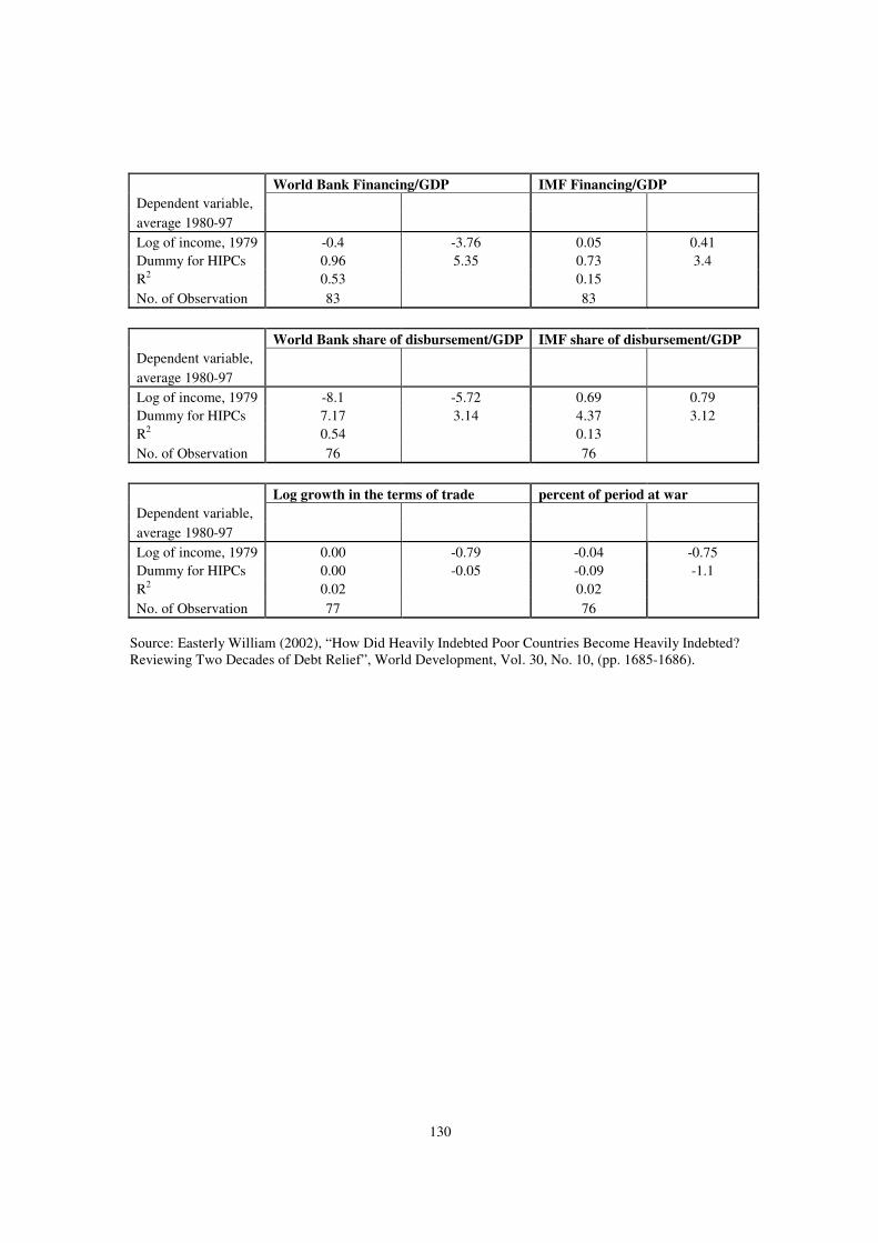
130
World Bank Financing/GDP IMF Financing/GDP Dependent variable, average 1980-97 Log of income, 1979 -0.4 -3.76 0.05 0.41 Dummy for HIPCs 0.96 5.35 0.73 3.4 R2 0.53 0.15 No. of Observation 83 83 World Bank share of disbursement/GDP IMF share of disbursement/GDP Dependent variable, average 1980-97 Log of income, 1979 -8.1 -5.72 0.69 0.79 Dummy for HIPCs 7.17 3.14 4.37 3.12 R2 0.54 0.13 No. of Observation 76 76 Log growth in the terms of trade percent of period at war Dependent variable, average 1980-97 Log of income, 1979 0.00 -0.79 -0.04 -0.75 Dummy for HIPCs 0.00 -0.05 -0.09 -1.1 R2 0.02 0.02 No. of Observation 77 76
Source: Easterly William (2002), “ How Did Heavily Indebted Poor Countries Become Heavily Indebted? Reviewing Two Decades of Debt Relief” , World Development, Vol. 30, No. 10, (pp. 1685-1686).

131
2. Empirical results on determinants of external indebtedness (1982-99) Table (2.38) Annual Cross-section (All developing Countries)1
1982 1983 1984 1985 1986 1987 1988 1989 1990 CONS -1.06
(-0.43) 0.494 (0.19)
-0.822 (-0.33)
-0.676 (-0.28)
-2.361 (-1.09)
0.581 (0.22)
4.172 (1.56)
-1.375 (-0.48)
-0.191 (-0.05)
SDX 0.000 (0.19)
0.000 (1.44)
0.000 (0.34)
0.000 (0.38)
0.000 (0.32)
0.001 (1.04)
0.000 (1.50)
-0.000 (-0.17)
0.000 (0.73)
MGDP 0.009**
(2.13) 0.012**
(2.15) 0.010*
(1.97) 0.011**
(2.15) 0.012**
(2.28) 0.007 (1.29)
0.000 (0.05)
0.007 (1.15)
0.006 (0.99)
CFLX 0.001 (0.70)
0.003***
(2.77) -0.002 (-1.17)
0.000 (0.99)
0.001 (1.52)
0.002***
(2.89) 0.002 (1.51)
0.002*
(1.67) 0.002*
(1.63) LTOT 0.005
(-0.95) -0.019***
(-3.01) 0.006 (0.81)
0.000 (0.08)
-0.009**
(-2.69) 0.016***
(3.21) -0.014**
(2.22) 0.027***
(3.13) 0.007 (0.89)
TDSX 0.018***
(3.61) 0.023***
(3.99) 0.032***
(4.92) 0.030***
(4.14) 0.024***
(4.58) 0.022***
(3.63) 0.019***
(3.02) 0.012*
(1.62) 0.021**
(2.37) LGDP 1.110***
(6.72) 0.942***
(5.39) 1.012***
(5.76) 1.035***
(6.12) 1.256***
(8.65) 1.054***
(6.11) 0.826***
(4.87) 1.193***
(6.23) 1.064***
(4.64) GRGD 0.032**
(2.26) -0.020*
(-1.65) 0.006 (0.48)
-0.024*
(-1.91) -0.013 (-1.08)
-0.03***
(-3.35) -0.018 (-1.23)
-0.009 (-055)
-0.007 (-0.42)
LPOP -0.248*
(-1.92) -0.111 (-0.82)
-0.132 (-0.96)
-0.165 (-1.21)
-0.39***
(-3.19) -0.247*
(-1.85) -0.125 (-0.88)
-0.333**
(-2.04) -0.227 (-1.24)
HIPC 0.314 (1.30)
0.307 (1.35)
0.271 (1.12)
0.261 (1.09)
0.619***
(2.78) 0.408 (1.59)
0.089 (0.32)
0.655**
(2.29) 0.400 (1.14)
N 56 57 57 59 59 59 60 60 60 R2 0.90 0.91 0.91 0.90 0.93 0.91 0.88 0.86 0.81 1. Dependent variable is log of total external debt (annual)
Table (2.38) continues 1991 1992 1993 1994 1995 1996 1997 1998 CONS 0.350
(0.11) 0.629 (0.24)
0.303 (0.17)
-2.084 (-0.71)
-3.059 (-1.20)
2.578 (1.08)
2.004 (0.88)
1.174 (0.41)
SDX 0.000 (0.32)
0.002 (0.55)
0.001 (0.59)
0.000 (0.04)
-0.000 (-0.25)
0.0001*
(1.81) 0.000 (1.53)
0.000 (0.61)
MGDP 0.004 (0.63)
0.004 (0.76)
0.005 (0.84)
0.008 (1.48)
0.007 (1.46)
0.003 (0.68)
0.005 (1.23)
0.002 (0.45)
CFLX 0.000 (0.11)
0.000 (0.02)
0.000 (0.05)
0.001 (1.23)
0.001 (0.58)
0.000 (-0.33)
-0.003*
(-1.79) 0.000 (0.23)
LTOT -0.003 (-0.54)
-0.001 (-0.13)
-0.008 (-0.63)
-0.004 (-0.52)
0.010 (1.23)
0.021***
(3.87) -0.016**
(-2.17) -0.005 (0.22)
TDSX 0.011**
(1.98) 0.018*
(1.89) 0.013 (1.48)
0.021***
(3.13) 0.016**
(1.99) 0.033***
(3.77) 0.029***
(3.45) 0.021**
(2.37) LGDP 0.955***
(4.57) 0.949***
(5.21) 0.955***
(4.87) 1.142***
(5.64) 1.204***
(6.84) 0.859***
(5.23) 0.874***
(5.11) 0.921***
(4.65) GRGD 0.007
(0.38) -0.001 (-0.07)
-0.005 (-0.26)
-0.009 (-0.94)
0.014 (1.33)
-0.0100 (-0.52)
-0.008 (-0.59)
-0.029 (-1.42)
LPOP -0.08 (-0.48)
-0.100 (-0.63)
-0.082 (-0.50)
-2.226 (-1.39)
-0.266*
(-1.77) -0.097 (-0.75)
-0.080 (-0.59)
-0.083 (-0.55)
HIPC 0.492 (1.51)
0.567*
(1.72) 0.578 (1.61)
0.553*
(1.79) 0.728**
(2.51) 0.472*
(1.85) 0.466*
(1.83) 0.441 (1.53)
N 60 58 57 57 57 56 55 52 R2 0.85 0.86 0.85 0.89 0.89 0.92 0.92 0.90

132
Table (2.39) Annual Cross-section (All developing Countries)2 1982 1983 1984 1985 1986 1987 1988 1989 1990 CONS 4.351*
(1.78) 5.620**
(2.39) 2.878 (1.33)
4.143**
(2.21) 3.581*
(1.73) 4.827**
(2.11) 7.419***
(3.16) 2.463 (0.96)
2.899 (0.99)
SDX 0.000 (0.31)
0.000 (1.03)
0.000 (-0.16)
0.000 (-0.35)
0.000 (-0.17)
0.000 (0.16)
0.000 (0.38)
0.000 (-1.22)
0.000 (-0.88)
MGDP 0.007*
(1.68) 0.006 (1.42)
0.011**
(2.49) 0.011***
(3.01) 0.010**
(2.08) 0.005 (1.05)
0.003 (0.65)
0.008 (1.58)
0.010*
(1.91) CFLX 0.002
(1.36) 0.000 (0.55)
-0.001 (-0.59)
-0.000 (-0.35)
0.000 (-0.24)
0.002***
(2.98) 0.001 (0.96)
0.002**
(2.39) 0.003***
(3.14) LTOT -0.006
(-0.97) -0.009 (-1.59)
-0.002 (-0.26)
0.007 (1.46)
-0.003 (-0.92)
0.015***
(3.38) -0.016***
(-2.99) 0.021***
(2.65) 0.009 (1.19)
TDSX 0.016**
(3.16) 0.026***
(4.76) 0.031***
(5.47) 0.032***
(5.69) 0.022***
(4.39) 0.015***
(2.95) 0.011**
(2.02) 0.012 (1.61)
0.021**
(2.62) LGDP 0.018
(0.11) -0.132 (-0.87)
0.066 (0.044)
0.021 (0.02)
0.081 (0.58)
0.035 (0.23)
-0.176 (-1.18)
0.184 (1.05)
0.086
(0.43) GRGD 0.016
(1.12) -0.009 (-.79)
-0.005 (-0.43)
-0.015 (-1.53)
0.002 (0.22)
-0.021**
(-2.36) -0.03**
(-2.32) -0.003 (-0.22)
0.000 (-0.01)
LPOP -0.112 (-0.87)
0.025 (0.20)
-0.098 (-0.83)
-0.075 (-0.72)
-0.151 (-1.27)
-0.122 (-1.06)
0.049 (0.39)
-0.207 (-1.40)
-0.113 (-0.71)
HIPC 0.299 (1.24)
0.268 (1.25)
0.291 (1.40)
0.168 (0.91)
0.251 (1.16)
0.198 (0.88)
0.024 (0.10)
0.518**
(2.00) 0.277 (0.99)
N 55 56 57 59 59 59 60 60 60 R2 0.36 0.43 0.49 0.54 0.39 0.46 0.44 0.36 0.44 2. Dependent variable is log of total external debt as a ratio to GDP (LEDTGDP)
Table (2.39) continues 1991 1992 1993 1994 1995 1996 1997 1998 CONS 5.275**
(2.06) 6.034***
(2.69) 5.221**
(2.01) 3.556 (1.32)
2.419 (1.01)
8.731***
(3.91) 7.531***
(3.35) 6.00**
(2.07) SDX 0.000
(-0.45) 0.000 (-0.02)
0.000 (-0.11)
0.000 (-1.05)
0.000 (-1.31)
0.000 (0.98)
0.000 (0.86)
0.000 (0.39)
MGDP 0.008*
(1.66) 0.009*
(1.86) 0.011**
(2.01) 0.011**
(2.05) 0.013***
(2.77) 0.009**
(2.37) 0.010***
(2.66) 0.011 (2.14)
CFLX 0.001 (0.57)
0.002*
(1.71) 0.002 (0.94)
0.001*
(1.64) 0.000 (-0.68)
-0.001**
(-2.37) -0.002 (-1.50)
0.000 (-0.11)
LTOT -0.001 (-0.24)
0.002 (0.33)
-0.004 (-0.37)
0.001 (0.22)
0.006 (0.78)
0.010*
(1.98) -0.011 (-1.63)
0.002 (0.30)
TDSX 0.019***
(4.29) 0.025***
(3.06) 0.015*
(1.87) 0.014**
(2.22) 0.016**
(2.18) 0.033***
(4.01) 0.024***
(3.02) 0.016*
(1.89) LGDP -0.172
(-0.98) -0.234 (-1.48)
-0.235 (-1.30)
-0.084 (-0.44)
-0.034 (-0.21)
-0.439***
(-2.83) -0.344**
(-2.14) -0.291 (-1.47)
GRGD -0.014 (-0.86)
0.000 (-0.01)
-0.007 (-0.44)
0.002 (0.23)
0.009 (0.91)
-0.009 (-0.48)
-0.010 (-0.45)
-0.027 (-1.31)
LPOP 0.142 (0.98)
0.164 (1.18)
0.227 (1.49)
0.109 (0.72)
0.091 (0.64)
0.305**
(2.49) 0.243*
(1.92) 0.234*
(1.73) HIPC 0.241
(0.87) 0.351 (1.23)
0.463 (1.40)
0.725**
(2.53) 0.811***
(2.98) 0.339 (1.41)
0.496**
(2.02) 0.527*
(1.83) N 60 58 57 57 57 56 55 52 R2 0.52 52 0.50 0.62 0.47 0.67 0.54 0.50

133
2.1. Panel results on determinants of external indebtedness (1982-99) Table (2.40a) Descriptive Statistics (All developing countries) Variable Observation Mean Std. Dev. Min Max LEDT 180 22.29 1.60 18.47 25.93 LEDTGDP 180 4.12 0.64 2.59 6.45 SDXI 179 885.41 2113.67 0.06 14380
CFLXI 179 26.08 84.97 -242.69 812.09
TDSXI 180 23.54 15.45 0.22 81.75
LTOTGI 178 -0.68 12.80 -83.19 48.75
MDGDPI 180 36.22 21.71 2.98 126.18
LGDPI 180 23.22 1.70 19.64 28.08
GRGDPI 179 6.51 7.63 -49.64 27.42
LPOP 180 16.05 1.55 19.77 28.24
Table (2.40b) Correlation Matrix (standard errors in parenthesis) (All developing countries) Variables LEDT SDX CFLX TDSX LTOTG MDGDP LGDP GRGDP LEDT 1.00 SDX 0.546*
(0.000) 1.00
CFLX 0.105 (0.16)
-0.049 (0.52)
1.00
TDSX 0.413*
(0.000) 0.032
(0.642) -0.042 (0.56)
1.00
LTOTG -0.082 (0.27)
-0.018 (0.81)
-0.013 (0.72)
-0.026 (0.72)
1.00
MDGDP -0.452*
(0.000) -0.072 (0.32)
0.063 (0.39)
-0.357*
(0.000) -0.023 (0.75)
1.00
LGDP 0.917*
(0.000) 0.557*
(0.000) 0.014 (0.85)
0.283*
(0.000) -0.018 (0.80)
-0.535*
(0.000) 1.00
GRGDP 0.053 (0.48)
0.081 (0.27)
-0.017 (0.82)
0.014 (0.85)
0.073 (0.33)
0.028 (0.70)
0.069 (0.35)
1.00
• Significant at 5 % level • Numbers in parentheses are standard errors

134
Table (2.40c) Correlation Matrix (standard errors in parenthesis) (All developing countries) Variables LEDT-
GDP SDX CFLX TDSX LTOTG MGDP LGDP GRGDP
LEDTG 1.00 SDX -0.210*
(0.004) 1.00
CFLX 0.364*
(0.000) -0.049 (0.515)
1.00
TDSX 0.307*
(0.000) 0.031
(0.673) 0.042
(0.569) 1.00
LTOTG -0.168*
(0.024) -0.018 (0.810)
-0.013 (0.863)
-0.026 (0.721)
1.00
MGDP 0.192*
(0.009) -0.073 (0.326)
0.063 (0.399)
-0.357*
(0.000) -0.023 (0.755)
1.00
LGDP -0.287*
(0.000) 0.557*
(0.000) 0.014
(0.849) 0.289*
(0.000) -0.018 (0.803)
-0.532*
(0.000) 1.00
GRGDP -0.083 (0.268)
0.081 (0.279)
-0.017 (0.816)
0.013 (0.854)
0.073 (0.330)
0.028 (0.703)
0.069 (0.355)
1.00
• = significant at 5 % • Numbers in parentheses are standard errors

135
Table (2.41a)
Panel regression results (1982-98)3
Random Effects Model Fixed Effects Model Variable 1 2 3 4 5 6 7 8
Const 2.844**
(2.01)
2.968**
(2.31)
2.64**
(2.13)
2.361*
(1.90)
21.46
(2.79)
16.61**
(2.38)
17.89**
(2.53)
18.36**
(2.53)
SDX 0.0001***
(3.42)
0.0001***
(3.59)
0.0001***
(3.34)
0.00006***
(3.19)
0.00007***
(3.35)
0.0001***
(3.47)
0.0001***
(3.40)
0.0001***
(3.29)
CFLX 0.0008**
(2.96)
0.001**
(2.94)
0.0008***
(2.90)
0.0007**
(2.38)
0.0007**
(2.37)
0.0007**
(2.34)
TDSX 0.003*
(1.74)
0.0029*
(1.85)
0.0017
(1.13)
0.0018
(1.23)
LTOTG -0.0024*
(-1.65)
-0.002
(-1.55)
MGDP 0.0042**
(2.11)
0.0017
(0.92)
0.0022
(1.15)
0.0023
(1.17)
0.004*
(1.86)
0.0014
(0.78)
0.0017
(0.84)
0.0017
(0.88)
LGDP 0.725***
(7.45)
0.757***
(8.28)
0.790***
(8.73)
0.815***
(8.90)
0.350***
(2.72)
0.478***
(4.00)
0.464***
(3.87)
0.474***
(3.75)
GRGDP -0.006*
(-1.92)
-0.008***
(-2.79)
-0.007**
(-2.47)
-0.0069**
(-2.01)
-0.0026
(-0.82)
0.006*
(-1.92)
-0.005*
(-1.70)
-0.004
(-1.29)
LPOP 0.129
(1.28)
0.079
(0.82)
0.044
(0.48)
0.024
(0.25)
-0.458
(-1.06)
-0.343
(0.78)
-0.405
(-1.02)
-0.449
(-1.12)
PD1 -0.072
(-1.06)
-0.007
(-0.109)
0.002
(0.03)
0.007
(0.11)
-0.509
(-3.27)
-0.339**
(-2.36)
-0.371**
(-2.54)
-0.379**
(-2.51)
PD2 0.065
(1.29)
0.091*
(1.98)
0.078
(1.58)
0.070
(1.39)
-0.134*
(-1.64)
-0.060
(-0.80)
-0.084
(-1.09)
-0.099
(-1.22)
HIPC 0.253
(1.25)
0.248
(1.27)
0.264
(1.45)
0.295*
(1.63)
N 178 177 177 177 178 177 177 176
R2 0.84 0.85 0.86 0.87 0.01 0.52 0.37 0.28
Prob(chi
2)a
0.001 0.009 failed failed
3. Dependent variable is log of total external debt (LEDT) a. the Hausman test in the first two columns is in favor of the fixed effects model.

136
Table (2.41b)
Panel regression results for all developing countries (1982-98)4 Random Effects Model Fixed Effects Model Variable 1 2 3 4 5 6 7 8
Const 6.222***
(4.15)
6.753***
(4.79)
7.121***
(5.39)
6.848***
(5.26)
-5.366
(-0.43)
-13.721
(-1.23)
-9.112
(-0.83)
-10.145
(-0.90)
SDX 0.00005*
(1.79)
0.00005**
(2.09)
0.00005*
(1.93)
0.00004*
(1.68)
0.0001**
(2.85)
0.0001***
(2.95)
0.0001***
(2.87)
0.0001***
(2.78)
CFLX 0.0014***
(3.47)
0.0015***
(3.59)
0.0014***
(3.58)
0.001**
(2.26)
0.001**
(2.29)
0.001**
(2.29)
TDSX 0.0095***
(4.16)
0.0098***
(4.32)
0.0062**
(2.68)
0.006***
(2.69)
LTOTG -0.004**
(-2.19)
-0.0064
(-1.35)
MGDP 0.0056**
(2.02)
0.0025
(0.98)
0.0037
(1.51)
0.0039*
(1.61)
0.0071**
(2.14)
0.0032
(1.04)
0.0039
(1.30)
0.0038
(1.25)
LGDP -0.218**
(-1.99)
-0.213***
(-2.05)
-0.236**
(-2.44)
-0.214**
(-2.25)
-0.661**
(-3.18)
-0.454**
(-2.39)
-0.502***
(-2.70)
-0.447**
(-2.28)
GRGDP -0.011**
(-2.07)
-0.011***
(-2.69)
-0.009**
(-2.20)
-0.007*
(-1.73)
-0.0043
(-0.84)
-0.009**
(-2.00)
-0.007
(-1.58)
-0.0064
(-1.34)
LPOP 0.173*
(1.68)
0.137
(1.36)
0.136
(1.48)
1.118
(1.33)
1.154**
(2.22)
1.762**
(2.81)
1.540**
(2.49)
1.521**
(2.45)
PD1 -0.279**
(-3.11)
-0.187**
(-2.18)
-0.234***
(-2.78)
-0.23***
(2.77)
-0.237
(-0.95)
0.044
(0.19)
-0.072
(-0.32)
-0.046
(-0.19)
PD2 0.074
(0.98)
0.115*
(1.68)
0.040
(0.57)
0.020
(0.28)
0.118
(0.90)
0.241**
(2.02)
0.151
(1.25)
0.151
(1.19)
HIPC 0.415**
(2.19)
0.362**
(1.97)
0.256
(1.51)
0.281
(1.71)
N 178 177 177 176 178 177 177 176
R2 0.24 0.30 0.40 0.43 0.0004 0.006 0.001 0.003
Prob(chi
2)b
0.39 0.16 0.56 0.37
4. Dependent variable is Log total external debt to GDP ratio (LEDTGDP)
b. The Hausman test is in favor of the random effects model

137
Table (2.42) Regression results of cross-section pooled time series for all (1982-98)5
Variables 1 2 3 4
Const -2.88**
(-2.05) -2.564*
(-1.84) -0.724 (-0.54)
-0.609 (-0.46)
SDXI 9.06e-06 (0.32)
0.00001 (0.44)
0.00003 (1.14)
0.00003 (1.12)
CFLXI 0.0014**
(2.46) 0.0013***
(2.59) 0.0014**
(2.58) TDSXI 0.0165***
(5.25) 0.0162***
(5.19) LTOTGI -0.007**
(-2.29) MDGDPI 0.009***
(3.16) 0.0014***
(2.75) 0.0086***
(3.20) 0.0083***
(3.08) LGDPI 1.176***
(12.57) 1.174***
(12.69) 1.050***
(11.79) 1.051***
(11.92) GRGDPI -0.006
(-0.88) -0.0053 (-0.81)
-0.0037 (-0.62)
-0.0019 (-0.31)
LPOP -0.203***
(-2.56) -0.221***
(-2.79) -0.170**
(-2.29) -1.759**
(-2.40) PD1 0.205*
(1.64) 0.293**
(2.28) 0.157 (1.28)
0.150 (1.28)
PD2 0.144 (1.21)
0.181 (1.52)
0.054 (0.47)
0.026 (0.28)
HIPC 0.761***
(5.29) 0.698***
(4.84) 0.445***
(3.12) 0.450***
(3.18) N 178 177 177 176
R2 0.86 0.86 0.88 0.88
5. Dependent variable is log of total external debt (LEDT)

138
Table (2.43) Differences in covariates between HIPCs and Non-HIPCs (1982-98) Average values
Heavily Indebted Poor Countries (HIPCs)
Non-Heavily Indebted countries (NON-HIPCs) Differences between the means
1982-87 1988-93 1994-98 1982-87 1988-93 1994-98 1982-87 1988-93 1994-98 LEDTG 4.12 4.62 4.82 3.97 3.95 3.84 0.15 0.67 0.98 LPOP 15.74 15.91 16.05 16.02 16.15 16.26 -0.28 -0.25 -0.21 CFLX -10.63 52.99 119.26 -1.36 9.86 24.19 -9.26 43.13 95.07 SDX 53.25 27.88 46.88 1580.95 772.20 1641.75 -1527.7 -744.33 -1594.8 MGDP 32.67 30.12 38.92 37.20 35.84 39.38 -4.54 -5.72 -0.46 LGDP 22.34 22.75 22.92 23.64 24.15 24.49 -1.30 -1.40 -1.58 GRGDP 4.18 11.33 2.63 2.60 10.90 6.66 1.58 0.43 -4.03 TDSX 23.95 32.03 27.06 23.15 23.79 17.02 0.79 8.24 10.04 LTOTG 2.70 -4.50 1.60 -3.72 0.61 0.39 6.42 -5.11 1.21
Table (2.44) The impact of each variable on the difference in the log of total external debt to GDP ratio between HIPCs and Non-HIPCs (1982-98)
Random effects model Fixed effects model 1982-87 1988-93 1994-98 1982-87 1988-93 1994-98 LPOP 0.70 0.60 0.50 12.60 0.11 9.59 CFLX 1.30 6.00 13.30 1.00 4.31 9.50 SDX 6.10 3.00 6.40 15.20 7.41 15.94 MGDP 1.80 2.20 0.20 1.00 1.00 0.07 LGDP 27.70 29.90 33.70 58.00 62.31 70.48 GRGDP 1.10 0.30 2.80 1.00 0.17 1.61 TDSX 0.80 8.10 9.80 0.47 4.97 6.02 LTOTG 1.50 1.20 0.30 1.00 1.00 0.24
The effects of each variable on the difference in total external debt to GDP ratio between HIPCs and Non-HIPCs was calculated as follows (I follow Klasen (2002): First, I take the difference in each covariates between the two groups as shown in table (2.43) . Second I take the regression coefficients of each covariate from column 4 and 8 of table 2.3d for the random and fixed effects models, respectively. Finally I multiplied the coefficients by the differences.

139
2.2. Panel results for determinants of indebtedness (HIPCs’) (1982-99) Table (2.45a) Descriptive Statistics (for HIPCs) Variable Observation Mean Std. Dev. Min Max LEDT 63 21.70 0.93 19.29 23.57 LEDTG 63 4.52 0.69 2.99 6.45 LPOP 63 15.89 0.76 14.37 17.88 MGDP 63 33.90 16.99 2.98 90.91 GRGDP 62 8.50 9.73 -16.5 49.2 LGDP 63 22.66 0.79 20.71 24.1 SDX 63 64.75 139.81 0.15 1020.71 CFLX 62 54.74 127.24 -85.80 812.09 LTOG 62 -0.06 19.28 -83.19 48.37 Table (2.45b) Correlation Matrix (standard errors in parentheses)-HIPCs
LEDT SDX MGDP CFLX TDSX LTOTG LGDP GRGDP LEDT 1.00 SDX -0.124
(0.33) 1.00
MGDP 0.069 (0.58)
-0.079 (0.54)
1.00
CFLX 0.289*
(0.02) 0.054 (0.67)
0.210 (0.10)
1.00
TDSX 0.394*
(0.001) 0.033 (0.79)
-0.061 (0.63)
-0.009 (0.94)
1.00
LTOTG -0.215 (0.09)
0.152 (0.23)
-0.084 (0.517)
-0.046 (0.72)
0.046 (0.72)
1.00
LGDP 0.641*
(0.000) 0.036 (0.77)
-0.466*
(0.000) 0.164 (0.20)
0.179 (0.16)
-0.0009 (0.99)
1.00
GRGDP 0.021 (0.87)
0.130 (0.31)
0.449*
(0.000) -0.083 (0.52)
0.027 (0.83)
-0.072 (0.58)
-0.260*
(0.04) 1.00
• *. Significant at 5 % level • Numbers in parentheses are standard errors

140
Table (2.45c) Correlation Matrix (Standard errors in parenthesis) HIPCs LEDTG SDX MGDP CFLX TDSX LTOTG LGDP GRGDP LEDTG 1.00 SDX -0.209
(0.09) 1.00
MGDP 0.528*
(0.000) -0.079 (0.54)
1.00
CFLX 0.444*
(0.000) 0.054 (0.67)
0.210 (0.10)
1.00
TDSX 0.219 (0.08)
0.033 (0.79)
-0.062 (0.63)
-0.009 (0.94)
1.00
LTOTG -0.314*
(0.01) 0.153 (0.24)
-0.084 (0.52)
-0.046 (0.73)
0.046 (0.72)
1.00
LGDP -0.027 (0.83)
0.063 (0.78)
-0.467*
(0.000) 0.164 (0.20)
0.179 (0.16)
-0.0009 (0.99)
1.00
GRGDP 0.103 (0.43)
0.130 (0.31)
-0.449*
(0.000) 0.083 (0.52)
0.028 (0.83)
-0.072 (0.58)
-0.260*
(0.04) 1.00
• *. Significant at 5% level • Numbers in parentheses are standard errors
Table (2.46a) Regression results for HIPC Panel (Cross-section pooled-time series) (1982-98)6
Variable 1 2 3 4 CONST -3.024
(-1.01) -2.407 (-0.80)
-1.441 (-0.52)
-1.062 (-0.39)
SDX -0.001*
(-1.78) -0.0011*
(-1.97) -0.001 (-2.15)
-0.0009*
(-1.83) CFLX 0.0011
(1.51) 0.011*
(1.68) 0.0011*
(1.66) TDSX 0.014***
(3.26) 0.0155***
(3.50) LTOTG -0.008**
(-2.13) MDGDP 0.0215***
(3.26) 0.0174**
(2.42) 0.0175**
(2.65) 0.0166**
(2.60) LGDP 1.219***
(6.55) 1.268***
(6.58) 1.176***
(6.55) 1.149***
(6.59) GRGDP 0.0099
(0.94) 0.013 (1.22)
0.0127 (1.25)
0.0117 (1.19)
LPOP -2.368 (-1.23)
-0.344 (-1.64)
-0.299 (-1.54)
-0.281 (1.49)
PD1 0.115 (0.52)
0.258 (1.07)
0.237 (1.08)
0.227 (1.04)
PD2 0.175 (0.86)
0.206 (1.00)
0.119 (0.62)
0.049 (0.26)
N 62 61 61 61 R2 0.62 0.63 0.70 0.72 6. Dependent variable is Log of total external debt (LEDT) 1982-98

141
Table (2.46b) Regression results for HIPC Panel (Cross-section pooled-time series) (1982-98)7
Variable 1 2 3 4 CONST 2.025
(0.82) 2.891 (1.21)
3.381 (1.45)
3.879*
(1.73) SDX -0.0007
(-1.42) -0.0008*
(-1.81) -0.0008*
(-1.84) -0.0006 (-1.46)
CFLX 0.0013**
(2.17) 0.0013**
(2.25) 0.0012**
(2.31) TDSX 0.0075*
(1.96) 0.082**
(2.27) LTOTG -0.0086***
(-2.83) MDGDP 0.0285***
(5.21) 0.0244***
(4.28) 0.0244***
(4.40) 0.023***
(4.51) LGDP 0.046
(0.29) 0.060 (0.39)
0.0134 (0.09)
-0.016 (-0.11)
GRGDP -0.022**
(-2.49) -0.020**
(-2.28) -0.0204**
(-2.39) -0.0214***
(-2.67) LPOP 0.054
(0.34) -0.0198 (-0.11)
0.0033 (0.20)
0.022 (0.14)
PD1 -0.582***
(-3.19) -0.402 (-2.12)
-0.413**
(-2.24) -0.423**
(-2.44) PD2 0.123
(0.73) 0.167 (1.03)
0.1234 (0.77)
0.048 (0.32)
N 62 61 61 61 R2 0.52 0.56 0.59 0.65 7. Dependent variable is Log of total external debt to GDP ratio (LEDTG)

142
A. The Magnitude of External Debt Table A1 Total external debt (Millions of USD)12 Years All ECA MENA EAP LAC SA SSA HIPCs
1982 808,321 87,254 110,587 129,376 354,834 49,431 76,838 74,450 1983 878,046 90,362 114,749 145,064 385,220 55,726 86,925 81,777 1984 919,499 105,863 116,507 153,088 395,485 57,505 91,050 87,113 1985 1,033,583 139,396 135,672 175,105 408,536 67,781 107,092 104,732 1986 1,132,428 157,362 153,532 193,144 428,523 79,040 120,827 117,447 1987 1,284,462 185,821 175,702 213,688 469,128 92,374 147,750 139,600 1988 1,286,654 185,986 179,195 214,979 456,324 99,912 150,257 142,675 1989 1,355,837 198,706 188,932 241,223 453,286 116,619 157,072 168,754 1990 1,460,343 220,428 183,205 274,071 475,867 129,899 176,873 189,854 1991 1,547,010 239,050 187,258 308,182 493,051 136,096 183,374 195,531 1992 1,621,514 253,198 188,321 344,546 509,798 142,961 182,689 200,908 1993 1,777,528 308,939 193,661 383,106 548,994 148,012 194,817 205,512 1994 1,969,044 326,029 208,223 463,076 588,279 162,129 221,308 216,923 1995 2,139,456 352,457 211,182 530,546 652,539 157,371 235,360 223,914 1996 2,229,400 369,566 204,844 591,348 676,286 155,522 231,833 217,957 1997 2,326,457 390,507 194,438 648,931 714,256 155,259 223,067 205,076 1998 2,536,046 480,539 208,059 667,522 786,019 163,775 230,132 213,960
12. Total external debt is the sum of public, publicly guaranteed, and private non-guaranteed long-term debt, use of IMF credit, and short-term debt. Source: Global Development Finance Table A2 Share of each group’ s debt in total developing countries’ debt (%) ECA MENA EAP LAC SA SSA HIPCs
1982 10.79 13.68 16.01 43.90 6.12 9.51 9.21 1983 10.29 13.07 16.52 43.87 6.35 9.90 9.31 1984 11.51 12.67 16.65 43.01 6.25 9.90 9.47 1985 13.49 13.13 16.94 39.53 6.56 10.36 10.13 1986 13.90 13.56 17.06 37.84 6.98 10.67 10.37 1987 14.47 13.68 16.64 36.52 7.19 11.50 10.87 1988 14.46 13.93 16.71 35.47 7.77 11.68 11.09 1989 14.66 13.93 17.79 33.43 8.60 11.58 12.45 1990 15.09 12.55 18.77 32.59 8.90 12.11 13.00 1991 15.45 12.10 19.92 31.87 8.80 11.85 12.64 1992 15.61 11.61 21.25 31.44 8.82 11.27 12.39 1993 17.38 10.89 21.55 30.89 8.33 10.96 11.56 1994 16.56 10.57 23.52 29.88 8.23 11.24 11.02 1995 16.47 9.87 24.80 30.50 7.36 11.00 10.47 1996 16.58 9.19 26.52 30.33 6.98 10.40 9.78 1997 16.79 8.36 27.89 30.70 6.67 9.59 8.81 1998 18.95 8.20 26.32 30.99 6.46 9.07 8.44
Source: own calculations based on Global Development Finance, 2000 (CD-ROM)

143
Table A3 Total debt (EDT)/GNP (%)13
All EAP ECA HIPCs LAC MENA SA SSA 1982 26.10 26.81 .. .. 45.16 27.66 19.09 32.19 1983 28.98 28.34 .. .. 57.19 27.06 20.34 38.57 1984 30.38 27.64 .. 71.54 60.89 27.20 21.12 44.20 1985 32.77 29.13 .. 81.15 60.65 30.56 22.92 56.37 1986 34.40 32.26 .. 63.51 60.16 33.69 25.24 58.48 1987 38.24 35.08 .. 85.80 64.84 43.54 26.56 60.98 1988 35.03 29.43 .. 88.78 55.22 46.70 26.80 59.55 1989 33.88 28.72 16.06 106.10 48.71 48.18 31.02 61.41 1990 34.19 29.81 18.56 118.78 44.35 42.84 32.02 63.01 1991 35.50 30.24 20.78 123.45 43.49 44.46 37.61 63.68 1992 35.89 30.65 24.78 137.32 39.55 41.89 39.94 62.91 1993 38.00 31.58 31.28 141.91 39.68 43.15 38.99 70.99 1994 39.42 32.07 37.86 166.59 37.83 47.57 37.38 82.57 1995 37.58 30.18 36.27 147.79 38.24 44.57 32.60 77.57 1996 35.72 29.95 33.57 129.77 37.55 38.34 29.74 73.82 1997 36.03 32.92 34.70 113.45 37.28 33.74 28.30 67.74 1998 42.14 40.16 48.59 114.64 40.83 36.05 29.22 72.32
13. Total debt to gross national product ratio (%)
Source: Global Development Finance 2000, CD-ROM Table A4 Total debt (EDT)/XGS (%)3
All EAP ECA HIPCs LAC MENA SA SSA 1982 127 117 - 252 278 60 209 121 1983 146 129 - 289 313 74 214 142 1984 148 121 - 286 289 84 210 145 1985 175 142 - 350 311 111 262 171 1986 209 148 - 393 369 168 289 215 1987 203 128 - 447 360 172 296 227 1988 181 106 - 437 308 173 296 222 1989 174 108 - 487 274 160 311 219 1990 162 108 - 501 256 114 327 210 1991 165 107 - 544 261 117 315 225 1992 159 105 129 556 251 113 317 223 1993 165 105 148 579 249 123 285 246 1994 158 103 135 552 230 135 262 273 1995 140 93 115 459 213 121 216 243 1996 132 95 108 391 201 103 195 218 1997 128 94 107 350 192 97 183 205 1998 148 105 134 378 210 129 189 239
14. Total debt to exports of goods and services ratio (%) Source: Global Development Finance, 2000 (CD-ROM)

144
B. The Costs of External debt Table B1 Debt service (TDS)/Exports of goods and services (XGS) (%)15
All EAP ECA HIPCs LAC MENA SA SSA 1982 19.17 18.01 .. 21.06 46.68 9.32 14.70 12.11 1983 19.27 18.27 .. 20.16 41.03 12.35 17.24 13.32 1984 19.93 18.28 .. 20.41 38.70 13.27 17.67 15.83 1985 23.03 23.84 .. 22.49 36.97 14.62 22.17 17.58 1986 26.53 23.92 .. 26.22 41.88 20.85 28.84 17.25 1987 24.23 24.74 .. 25.39 36.02 17.44 27.81 13.52 1988 23.26 18.90 .. 24.72 36.90 19.43 26.28 14.86 1989 20.63 16.72 .. 21.92 30.19 19.03 26.49 13.12 1990 18.27 15.73 .. 21.14 24.50 15.10 29.00 12.92 1991 17.36 13.35 .. 21.63 24.20 15.31 25.61 12.46 1992 16.40 13.51 11.34 17.10 26.11 15.54 25.01 12.28 1993 16.24 14.06 10.01 17.70 27.71 14.60 22.84 9.20 1994 15.89 12.09 11.88 18.95 25.29 14.53 25.23 14.57 1995 15.76 11.43 12.20 20.73 26.46 13.72 24.96 15.29 1996 16.46 12.11 11.46 15.87 31.49 12.64 20.80 14.22 1997 17.15 11.21 11.54 15.41 35.93 12.55 20.99 14.72 1998 18.43 13.32 14.72 16.41 33.56 14.04 18.92 14.68
15. Total debt service is the sum of principal repayments and interest actually paid in foreign currency, goods, or services on long-term debt, interest paid on short-term debt and repayments (repurchases and charges) to the IMF Table B2 Interest (INT)/Exports of goods and services (XGS) (%)16
All EAP ECA HIPCs LAC MENA SA SSA 1982 11 11 - 12 30 4 8 7 1983 11 10 - 11 28 4 9 7 1984 11 10 - 11 26 5 10 8 1985 12 10 - 11 27 6 11 8 1986 12 10 - 11 26 8 12 7 1987 11 8 - 10 22 6 12 6 1988 11 7 - 10 22 8 11 7 1989 9 7 - 9 16 8 14 6 1990 8 6 - 9 12 5 16 6 1991 8 6 - 9 13 5 14 6 1992 7 5 5 7 11 6 12 6 1993 6 5 4 8 11 6 11 4 1994 6 4 4 8 11 6 10 6 1995 7 5 5 7 12 6 9 6 1996 6 5 5 6 12 5 8 5 1997 6 5 5 6 11 5 8 5 1998 7 5 5 6 12 6 8 5
16. payments made to domestic sectors and to nonresidents for the use of borrowed money.
Source (for tables B1 and B2): Global Development Finance 2000, CD-ROM

145
Table B3 Interest (INT)/GNP (%)
All EAP ECA HIPCs LAC MENA SA SSA 1982 2.26 2.42 - - 4.82 1.89 0.71 1.77 1983 2.17 2.17 - - 5.18 1.63 0.83 1.82 1984 2.33 2.27 - 2.70 5.46 1.65 0.96 2.37 1985 2.30 2.14 - 2.46 5.20 1.54 0.96 2.49 1986 2.05 2.08 - 1.84 4.27 1.53 1.05 1.97 1987 1.98 2.15 - 1.94 3.97 1.63 1.09 1.53 1988 2.05 1.92 - 2.04 4.03 2.05 1.04 1.87 1989 1.81 1.83 0.97 1.96 2.79 2.33 1.40 1.78 1990 1.65 1.66 1.04 2.07 2.13 2.01 1.53 1.89 1991 1.66 1.65 1.05 2.14 2.13 1.91 1.64 1.82 1992 1.52 1.47 0.89 1.80 1.79 2.17 1.53 1.58 1993 1.47 1.45 0.91 1.85 1.76 1.98 1.44 1.22 1994 1.57 1.39 1.17 2.30 1.84 1.96 1.41 1.78 1995 1.77 1.53 1.50 2.16 2.20 2.13 1.36 1.77 1996 1.71 1.47 1.46 1.96 2.21 1.84 1.16 1.86 1997 1.75 1.63 1.56 1.86 2.21 1.59 1.20 1.55 1998 2.00 2.03 1.93 1.96 2.41 1.55 1.20 1.65
Source: Global Development Finance, 2000 (CD-ROM) C. The Structure of External Debt Table C1 The share of short-term debt in total external debt (%)17
All EAP ECA HIPCs LAC MENA SA SSA 1982 23.39 27.19 16.36 12.39 25.77 29.89 7.43 14.88 1983 18.61 25.56 15.94 11.47 16.23 27.19 8.44 15.52 1984 16.78 25.19 13.68 13.07 12.94 25.33 8.69 17.11 1985 15.83 22.35 15.63 14.22 11.17 24.46 8.96 16.60 1986 13.62 17.37 17.06 10.31 8.52 23.92 9.07 11.10 1987 13.24 15.73 17.00 10.85 9.58 21.67 9.04 9.14 1988 14.30 17.03 19.24 11.59 10.77 21.36 9.48 9.77 1989 15.70 16.42 21.52 12.02 13.14 23.13 9.27 10.47 1990 16.75 17.94 18.54 12.64 16.27 23.96 9.52 11.81 1991 17.16 19.23 16.44 12.81 17.61 24.69 8.74 11.97 1992 18.34 20.89 16.69 13.98 18.49 27.64 7.89 13.95 1993 18.37 22.05 13.69 14.39 20.18 27.60 4.09 15.10 1994 18.31 24.66 11.38 13.36 20.05 23.10 4.32 16.31 1995 19.84 28.97 12.94 13.83 20.03 21.11 5.77 17.32 1996 20.67 31.51 14.39 14.26 18.52 21.01 6.64 18.42 1997 20.17 28.31 14.89 13.20 19.18 21.21 5.30 18.37 1998 16.24 17.84 16.36 13.14 15.71 19.70 4.37 18.47
17. Short-term debt includes all debt having an original maturity of one year or less and interest in arrears on long-term debt.
Source: Global Development Finance, 2000(CD-ROM)
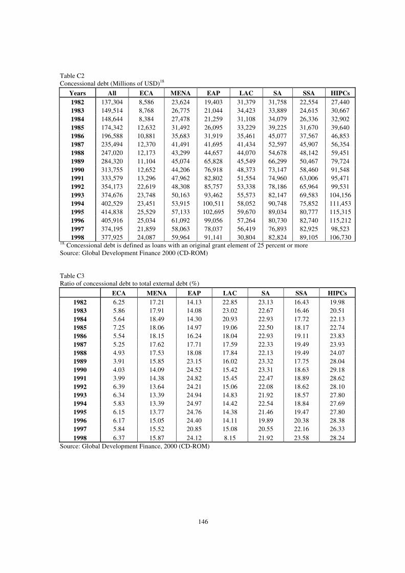
146
Table C2 Concessional debt (Millions of USD)18
Years All ECA MENA EAP LAC SA SSA HIPCs 1982 137,304 8,586 23,624 19,403 31,379 31,758 22,554 27,440 1983 149,514 8,768 26,775 21,044 34,423 33,889 24,615 30,667 1984 148,644 8,384 27,478 21,259 31,108 34,079 26,336 32,902 1985 174,342 12,632 31,492 26,095 33,229 39,225 31,670 39,640 1986 196,588 10,881 35,683 31,919 35,461 45,077 37,567 46,853 1987 235,494 12,370 41,491 41,695 41,434 52,597 45,907 56,354 1988 247,020 12,173 43,299 44,657 44,070 54,678 48,142 59,451 1989 284,320 11,104 45,074 65,828 45,549 66,299 50,467 79,724 1990 313,755 12,652 44,206 76,918 48,373 73,147 58,460 91,548 1991 333,579 13,296 47,962 82,802 51,554 74,960 63,006 95,471 1992 354,173 22,619 48,308 85,757 53,338 78,186 65,964 99,531 1993 374,676 23,748 50,163 93,462 55,573 82,147 69,583 104,156 1994 402,529 23,451 53,915 100,511 58,052 90,748 75,852 111,453 1995 414,838 25,529 57,133 102,695 59,670 89,034 80,777 115,315 1996 405,916 25,034 61,092 99,056 57,264 80,730 82,740 115,212 1997 374,195 21,859 58,063 78,037 56,419 76,893 82,925 98,523 1998 377,925 24,087 59,964 91,141 30,804 82,824 89,105 106,730
18. Concessional debt is defined as loans with an original grant element of 25 percent or more
Source: Global Development Finance 2000 (CD-ROM) Table C3 Ratio of concessional debt to total external debt (%)
ECA MENA EAP LAC SA SSA HIPCs 1982 6.25 17.21 14.13 22.85 23.13 16.43 19.98 1983 5.86 17.91 14.08 23.02 22.67 16.46 20.51 1984 5.64 18.49 14.30 20.93 22.93 17.72 22.13 1985 7.25 18.06 14.97 19.06 22.50 18.17 22.74 1986 5.54 18.15 16.24 18.04 22.93 19.11 23.83 1987 5.25 17.62 17.71 17.59 22.33 19.49 23.93 1988 4.93 17.53 18.08 17.84 22.13 19.49 24.07 1989 3.91 15.85 23.15 16.02 23.32 17.75 28.04 1990 4.03 14.09 24.52 15.42 23.31 18.63 29.18 1991 3.99 14.38 24.82 15.45 22.47 18.89 28.62 1992 6.39 13.64 24.21 15.06 22.08 18.62 28.10 1993 6.34 13.39 24.94 14.83 21.92 18.57 27.80 1994 5.83 13.39 24.97 14.42 22.54 18.84 27.69 1995 6.15 13.77 24.76 14.38 21.46 19.47 27.80 1996 6.17 15.05 24.40 14.11 19.89 20.38 28.38 1997 5.84 15.52 20.85 15.08 20.55 22.16 26.33 1998 6.37 15.87 24.12 8.15 21.92 23.58 28.24
Source: Global Development Finance, 2000 (CD-ROM)
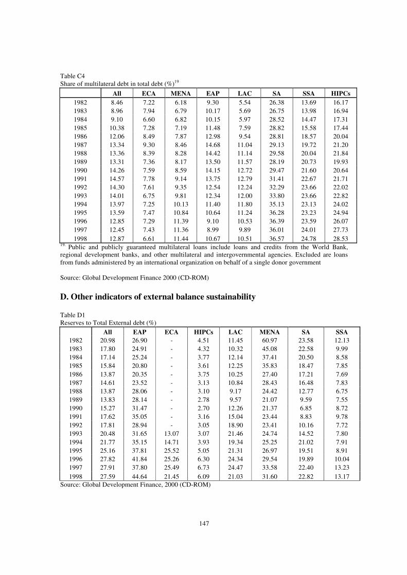
147
Table C4 Share of multilateral debt in total debt (%)19
All ECA MENA EAP LAC SA SSA HIPCs 1982 8.46 7.22 6.18 9.30 5.54 26.38 13.69 16.17 1983 8.96 7.94 6.79 10.17 5.69 26.75 13.98 16.94 1984 9.10 6.60 6.82 10.15 5.97 28.52 14.47 17.31 1985 10.38 7.28 7.19 11.48 7.59 28.82 15.58 17.44 1986 12.06 8.49 7.87 12.98 9.54 28.81 18.57 20.04 1987 13.34 9.30 8.46 14.68 11.04 29.13 19.72 21.20 1988 13.36 8.39 8.28 14.42 11.14 29.58 20.04 21.84 1989 13.31 7.36 8.17 13.50 11.57 28.19 20.73 19.93 1990 14.26 7.59 8.59 14.15 12.72 29.47 21.60 20.64 1991 14.57 7.78 9.14 13.75 12.79 31.41 22.67 21.71 1992 14.30 7.61 9.35 12.54 12.24 32.29 23.66 22.02 1993 14.01 6.75 9.81 12.34 12.00 33.80 23.66 22.82 1994 13.97 7.25 10.13 11.40 11.80 35.13 23.13 24.02 1995 13.59 7.47 10.84 10.64 11.24 36.28 23.23 24.94 1996 12.85 7.29 11.39 9.10 10.53 36.39 23.59 26.07 1997 12.45 7.43 11.36 8.99 9.89 36.01 24.01 27.73 1998 12.87 6.61 11.44 10.67 10.51 36.57 24.78 28.53
19. Public and publicly guaranteed multilateral loans include loans and credits from the World Bank, regional development banks, and other multilateral and intergovernmental agencies. Excluded are loans from funds administered by an international organization on behalf of a single donor government Source: Global Development Finance 2000 (CD-ROM) D. Other indicators of external balance sustainability Table D1 Reserves to Total External debt (%)
All EAP ECA HIPCs LAC MENA SA SSA 1982 20.98 26.90 - 4.51 11.45 60.97 23.58 12.13 1983 17.80 24.91 - 4.32 10.32 45.08 22.58 9.99 1984 17.14 25.24 - 3.77 12.14 37.41 20.50 8.58 1985 15.84 20.80 - 3.61 12.25 35.83 18.47 7.85 1986 13.87 20.35 - 3.75 10.25 27.40 17.21 7.69 1987 14.61 23.52 - 3.13 10.84 28.43 16.48 7.83 1988 13.87 28.06 - 3.10 9.17 24.42 12.77 6.75 1989 13.83 28.14 - 2.78 9.57 21.07 9.59 7.55 1990 15.27 31.47 - 2.70 12.26 21.37 6.85 8.72 1991 17.62 35.05 - 3.16 15.04 23.44 8.83 9.78 1992 17.81 28.94 - 3.05 18.90 23.41 10.16 7.72 1993 20.48 31.65 13.07 3.07 21.46 24.74 14.52 7.80 1994 21.77 35.15 14.71 3.93 19.34 25.25 21.02 7.91 1995 25.16 37.81 25.52 5.05 21.31 26.97 19.51 8.91 1996 27.82 41.84 25.26 6.30 24.34 29.54 19.89 10.04 1997 27.91 37.80 25.49 6.73 24.47 33.58 22.40 13.23 1998 27.59 44.64 21.45 6.09 21.03 31.60 22.82 13.17
Source: Global Development Finance, 2000 (CD-ROM)

148
Table D2 External Balance on Goods and services (Resource balance) (% GDP)20
ECA MENA EAP LAC SA SSA HIPCs 1982 - 0.53 -1.00 0.31 -5.09 -4.25 -7.95 1983 - -3.04 -1.49 3.45 -4.51 -1.24 -5.33 1984 - -7.92 -0.14 4.83 -4.23 -0.55 -3.71 1985 - -5.58 -1.39 4.66 -5.07 3.11 -3.93 1986 - -7.36 0.47 2.39 -4.52 2.38 -4.54 1987 - -4.45 2.49 2.68 -3.91 1.87 -6.05 1988 - -4.51 1.81 3.11 -4.41 0.65 -6.52 1989 0.80 -5.41 0.26 3.04 -3.76 1.03 -5.58 1990 -0.90 -1.78 0.26 2.12 -3.96 1.50 -5.90 1991 -0.45 -4.17 -0.09 0.39 -2.17 0.28 -5.21 1992 0.93 -2.81 0.11 -0.20 -2.87 -1.27 -6.35 1993 -0.76 -3.84 -1.04 -0.93 -2.90 -1.64 -7.60 1994 0.31 1.18 -0.20 -1.35 -3.46 -1.41 -6.66 1995 -0.84 0.77 -0.76 -0.90 -4.00 -1.59 -6.06 1996 -1.77 3.65 -1.22 -0.86 -4.78 0.59 -6.36 1997 -2.63 2.85 1.39 -2.16 -4.39 -1.26 -6.24 1998 -1.59 -2.91 8.69 -3.05 -3.24 -2.70 -7.10
20. The difference between exports of goods and services and imports of goods and services
Table D3 Share of each group (region) in total portfolio equity inflow (%)21
EAP ECA HPC LAC MNA SA SSA 1980 0.00 0.00 0.00 0.00 0.00 0.00 0.00 1981 28.19 0.00 0.00 71.81 0.00 0.00 0.00 1982 0.00 0.00 0.00 0.00 0.00 0.00 0.00 1983 0.00 0.00 0.00 0.00 0.00 0.00 0.00 1984 100.00 0.00 0.00 0.00 0.00 0.00 0.00 1985 100.00 0.00 0.00 0.00 0.00 0.00 0.00 1986 5.23 0.00 0.00 0.00 0.00 32.38 0.00 1987 46.36 0.00 0.00 11.37 0.00 0.00 0.00 1988 44.31 0.00 0.00 16.01 0.00 5.10 0.00 1989 77.79 2.11 0.00 12.87 0.00 4.98 0.00 1990 61.18 6.28 0.00 29.68 0.00 2.81 0.05 1991 15.88 0.00 0.13 83.79 0.00 0.30 0.03 1992 37.72 0.46 0.00 59.11 0.00 2.70 0.01 1993 40.67 1.93 0.17 53.39 0.00 3.97 0.04 1994 35.87 6.26 2.49 37.43 0.30 17.70 2.45 1995 50.68 7.57 1.22 21.20 0.56 6.49 13.50 1996 36.79 16.97 1.21 28.25 3.32 10.57 4.09 1997 30.45 15.93 -0.07 32.94 7.48 8.20 4.99 1998 57.85 18.65 0.31 11.23 5.64 2.25 4.37
21. Portfolio equity flows are the sum of country funds, depository receipts (American or global), and direct purchases of shares by foreign investors. Source: Own calculations based on data from Global Development Finance 2000

149
Table D4 Gross Domestic Savings (% GDP)
World ECA MENA EAP LAC SA SSA HIPCs 1982 23.19 NA 27.30 29.70 21.87 17.02 17.07 9.57 1983 22.70 NA 24.41 30.33 21.35 16.27 16.19 10.06 1984 23.40 NA 21.79 31.07 22.18 16.35 16.72 10.63 1985 23.22 NA 18.87 30.59 23.64 17.76 18.36 11.31 1986 22.86 NA 16.02 31.81 21.00 17.58 17.72 10.50 1987 23.31 NA 18.62 33.63 23.70 17.76 17.06 9.08 1988 24.08 NA 18.49 34.20 25.26 18.47 17.98 9.69 1989 24.64 31.43 21.27 34.01 25.01 19.10 17.88 8.93 1990 23.99 26.01 22.70 34.89 21.46 19.72 16.21 9.16 1991 23.54 27.50 20.95 35.46 19.86 19.61 15.41 9.90 1992 23.25 28.34 23.18 35.17 19.42 20.15 13.55 8.73 1993 22.77 24.68 21.08 36.83 19.76 18.23 14.52 8.71 1994 23.09 24.40 24.13 37.37 20.21 19.28 16.28 11.64 1995 23.21 23.97 25.25 37.10 20.38 20.88 16.69 12.18 1996 23.11 22.83 24.20 36.14 19.95 16.73 18.08 12.13 1997 23.43 21.45 24.28 36.53 19.85 18.11 15.96 12.40 1998 23.07 19.87 19.19 37.59 18.77 18.14 16.10 12.46
Source: World Development Indicators 2001, World Bank
Table D5 Gross domestic investment as a share of GDP (%)
World ECA MENA EAP LAC SA SSA HIPCs 1982 23.13 NA 26.83 28.13 21.40 19.88 22.83 16.34 1983 22.28 NA 27.73 28.82 17.81 19.09 21.11 14.95 1984 22.20 NA 26.46 28.23 16.93 19.13 19.13 13.90 1985 22.10 NA 23.88 27.56 17.22 19.92 18.20 13.41 1986 22.10 NA 22.94 27.76 18.79 20.28 17.65 14.24 1987 22.45 NA 22.11 28.36 20.60 20.76 17.03 14.19 1988 22.98 NA 21.21 28.94 21.38 20.53 18.52 14.39 1989 23.32 26.59 20.93 27.90 21.73 21.31 18.34 13.80 1990 23.17 24.83 20.92 30.16 19.30 21.78 17.92 14.48 1991 22.48 21.89 21.62 31.43 18.01 21.05 17.63 14.03 1992 22.20 22.59 22.23 32.41 18.64 21.56 16.52 14.29 1993 21.92 21.73 22.69 35.23 19.25 21.03 16.72 15.32 1994 21.99 22.28 22.02 34.72 20.36 21.32 17.16 17.78 1995 21.99 22.16 22.42 34.64 19.45 23.22 16.96 17.65 1996 22.18 22.59 21.06 34.68 18.96 22.09 16.90 18.26 1997 22.13 22.28 21.75 33.18 19.85 21.74 17.17 18.19 1998 21.87 21.44 20.90 30.10 20.32 20.69 18.51 18.72
Source: World Development Indicators 2001, World Bank

150
Table D6 Net resource flows and transfers of HIPCs and other developing countries (1984-98)22
Heavily indebted poor countries (HIPCs) All developing countries
Resource flows and transfers 1984-90 1991-98 1984-90 1991-98 Net flows on debt, total (% of GNP)a 4.928 2.852 1.377 2.182 Net transfers on debt, total (% of GNP)b 2.783 0.850 -0.646 0.504 Aggregate net resource flows (% of GNP)c 8.405 10.536 2.117 4.433 Aggregate net transfers (% of GNP)d 6.291 8.299 0.155 2.651 Official net resource flows (% of GNP)e 7.485 8.273 1.167 0.948 Official net transfers (% of GNP)f 6.612 7.099 0.747 0.454 Portfolio equity flows (% of GNP) 0.000 0.175 0.025 0.550 Private net resource flows (% of GNP)g 0.920 2.263 0.950 3.485 Private net transfers (% of GNP)h -0.321 1.199 -0.592 2.197
22 data for GNP for HIPCs is available only since 1984
a. Net flows on debt is disbursements on long-term debt and IMF purchases minus principal repayments on long-term debt and IMF repurchases up to 1984. Beginning in 1985 this line includes the change in stock of short-term debt (including interest arrears for long-term debt). b. Net transfers on debt are net flows minus interest payments (or disbursements minus total debt service payments). c. Aggregate net resource flows are the sum of net resource flows on long-term debt (excluding IMF) plus net direct foreign investment, portfolio equity flows and official grants (excluding technical cooperation). Net flows (or net lending or net disbursements) are disbursements minus principal repayments d. Aggregate net transfers are equal to aggregate net resource flows minus interest payments on long-term loans and foreign direct investment profits. e. Private net resource flows are the sum of net flows on debt to private creditors (PPG and PNG) plus net direct foreign investment and portfolio equity flows f. Official net transfers are equal to official net resource flows minus official interest payments on long-term loans. g. Private net resource flows are the sum of net flows on debt to private creditors (PPG and PNG) plus net
direct foreign investment and portfolio equity flows h. Private net transfers are equal to private net resource flows minus private interest payments on long-term loans (PPG and PNG) and foreign direct investment profits. Source: Own calculations based on data from Global Development Finance 2000, (CD-ROM)

III. Factors Affecting the Debt-Repayment
Capacity of Indebted Countries:
An Empirical Investigation

152
Abstract
The failure of indebted developing countries to meet their contractual debt obligations has been
one of the major concerns of the international community since the outset of the debt crisis in
1982. While poverty and external factors seem to be the most profound factors behind the
external indebtedness of poor nations, there is still an ongoing debate as to why indebted
countries have failed to manage servicing their external debt.
This paper, using cross-section pooled logit, probit and fixed effects logit models empirically
explores the determinants of rescheduling contractual debt service payments by developing
countries in the past two decades. The results seem to suggest that past external debt, the level of
income per capita, the growth rate of GDP, openness, the levels of international reserves and
capital inflows to be the core determining factors behind the behavior of borrowers towards
meeting their contractual debt obligations.
From the empirical strategy perspectives, as in the case of debt determinants, the application of a
panel data approach seems to be highly preferred, as it allows to control for time-specific events
that are linked to overseas borrowing, particularly given the rapid changes in the global
macroeconomic environment in the past years. Moreover, this strategy helps to produce a more
robust explanation by allowing to incorporate country-specific factors as developing countries
themselves are heterogeneous in terms of their colonial heritages, geopolitical and strategic
significance, and creditworthiness, all affecting the level of indebtedness and the potential
bargaining power to manage the subsequent debt crisis.

153
1. Introduction “ The debt crisis can be studied as a problem in epidemiology. A powerful virus, high world interest rate, hit the population of capital importing developing countries in the 1980s. Some countries succumbed to the virus, having to reschedule their debt on an emergency basis, while others did not. And of those countries that arrived for emergency treatment, some recovered sufficiently to enter the period of quiet convalescence, while others are still suffering from febrile seizures in the IMF’ s intensive care unit” , Sachs and Berg (1988, pp. 1)
The external debt crisis of developing countries’ is believed to be one of the major
challenges of the new millennium. As Eatwell and Taylor (2000, in: Dymski, 2002)
express it, “ international debt crisis has become a defining feature of the contemporary
world economy” .52 In this regard, McFadden, et al (1985, in Smith, et al (1985)), among
others, argue that the primary question in international debt crisis is why indebted
countries failed to meet their debt-service obligations. The late 1980s and the 1990s
witness that developing countries in general and HIPCs in particular have suffered from
chronic debt-servicing difficulties.53. Though it is generally believed that external debt
helps countries that are suffering from capital deficiency to achieve accelerated economic
growth, once this financial gap becomes unmanageable, the past accumulated external
debt is likely to provoke further external borrowing, creating a vicious circle problem.
This obviously creates a gloomy picture on future growth prospects and reduces the
likelihood of developing countries to meet their debt-service obligations, which is exactly
the current experience of the poorest nations of the world, earning the new name “ heavily
indebted poor countries” (HIPCs).
The debt-servicing difficulties of indebted poor countries are remarkable. For instance,
based on the Global Development Finance, 2000, interest arrears as a ratio to total long-
term debt outstanding for SSA and HIPCs in 1989 represent 5.3% and 7%, respectively.
52 As they put it, “ the past 8 years, a period of virtually unregulated cross-border financial flows, have witnessed 8 major episodes of international debt and financial crises: the 1994-95 Mexican “ Tequila” crisis, the 1997-98 Asian financial crises, the 1998-99 run on Brazilian real, the 1998-99 Russian ruble (long-term credit crisis, the 2000 Turkish crisis, the 2001-02 meltdown of the Argentine economy, the 2002 attack on the Brazilian real, and the 2002 Uruguayan collapse” . 53 The debt-servicing difficulty in fact became apparent already in August 1982, after Mexico’ s official announcement that it could no longer manage to continue servicing its external debt. This was the beginning of the end to the creditworthiness of most poor countries. Fafchamps (1996) defines debt crises in terms of ability to pay, where he argues that a country defaults on its debt because it has run out of foreign exchange (pp. 315).

154
In 1998, this ratio increased to 11% and 9% respectively. In 1989, principal arrears as a
share of total long-term outstanding for SSA and HIPCs were around 10% and 13%
respectively. In 1998, this ratio rose to 11% for SSA and nearly 24% for HIPCs. This is
in contrast to 3% for EAP and 1.2% for LAC. (See, table 3.1).
Table (3.1)
Arrears and rescheduling (% of total external debt (EDT) and GNP)
Heavily indebted poor countries All developing countries Debt crisis indicators 1984-90 1991-98 1984-90 1991-98 Total amount of debt rescheduled (% of EDT) 3.05 2.12 4.75 2.68 Principal rescheduled (% of EDT) 1.60 0.98 1.46 0.90 Principal forgiven (% of EDT) 0.65 1.01 0.22 0.20 Interest rescheduled (% of EDT) NA 0.57 NA 0.54 Interest forgiven (% of EDT) 0.07 0.26 0.03 0.04 Debt stock rescheduled (% of EDT) 0.38 0.21 2.78 1.08 Debt stock reduction (% of EDT) 0.08 0.65 0.61 0.50 Interest arrears on LDOD (% of EDT) 4.77 8.34 1.91 2.21 Principal arrears on LDOD (% of EDT) 8.25 19.22 2.87 4.37 Total amount of debt rescheduled (% of GNP) 2.65 2.80 1.66 1.00 Principal rescheduled (% of GNP) 1.38 1.31 0.50 0.33 Principal forgiven (% of GNP) 0.65 1.36 0.08 0.07 Interest rescheduled (% of GNP) NA 0.76 NA 0.20 Interest forgiven (% of GNP) 0.07 0.34 0.01 0.01 Debt stock rescheduled (% of GNP) 0.33 0.27 0.99 0.41 Debt stock reduction (% of GNP) 0.08 0.82 0.21 0.18 Interest arrears on LDOD (% of GNP) 4.36 11.30 0.65 0.82 Principal arrears on LDOD (% of GNP) 7.65 25.96 0.99 1.64 Total external debt (EDT) to GNP ratio 87.95 134.36 34.13 37.53
Source: Own calculations based on: Global Development Finance, 2000 CD-ROM and World Development Indicators, 2001 CD-ROM
From table (3.1), it is also apparent that HIPCs average principal arrears on loans reached
more than 8% of its total external debt in 1984-90, which rose to nearly 20% in the 1991-
98 period. Other developing countries have by far lower problems compared to those of
the HIPCs. Similarly, this ratio on average reached about 26% of HIPCs’ GNP, a clear
indication that this group has not managed to pay back its international debt obligations.
This ratio for other developing countries, again, on average, was around 1% in (1984-90)
and around 1.5% in the (1991-98) periods, respectively. Similarly, interest arrears on

155
loans are quite higher for HIPCs relative to other low and middle income countries. The
ratio of interest arrears to GDP reached around 5% in the 1984-89, which even nearly
doubled in the 1991-98 period. The difference is quite apparent that I need not to
elaborate that further.
The objective of this chapter is to empirically address the reasons behind the failure of
indebted countries in the 1980s and 1990s to fully service their contractual external debt
obligations.54 To answer the above question, the remainder of the paper is divided into
seven parts: Part 2 presents a brief summary of the factors that drive countries to debt
crises situations. Part 3 summarizes the past empirical studies in this area. Part 4
discusses the empirical specification of the model used to figure out the factors that cause
debt crisis. Part 5 briefly introduces the data and variables that are included in the
regression. Part 6 presents results and the discussion. Finally part 7 concludes and
presents the possible policy implications of the study.
Now, reiterating the question, the main issue I intend to address here is what are the main
factors that drive countries into a debt crisis situation? In other words, why have indebted
poor countries failed to service their external debt and instead opted for rescheduling?
Bearing this question in mind, and before I myself address these issues, I will briefly
summarize most relevant previous researchers results.
2. Factors affecting debt-repayment capacity: A theoretical review
Following McFadden, et al (1985, in Smith, et al (1985)), among others, generally a
country is said to be in a debt repayment crisis situation if it has arrears on principal or
interest, higher-tranche IMF arrangements, or rescheduling requests (p.188). From the
figures in table (3.1) it is apparent that HIPC’ s have failed to convert the resources they
obtained through overseas borrowing into growth and ultimately service their external
debt. However, although many of the indebted poor countries were in extremely difficult
54 Most of the theoretical explanations on the debt crisis in the preceding chapter are relevant to this chapter. I will mainly focus on the empirical counterpart of the explanation for the debt payment difficulties of indebted nations in the past two decades.

156
situations, they in principle remained committed to repay their external debt obligations.
This is in contrast to the debt crisis in the 1930s, where virtually every Latin American
country unilaterally suspended servicing its external bond obligations (Sachs, 1986).55It
appears that rescheduling rather than default is mutually beneficial both for debtors and
creditors. Marchesi (2000) argues in this line. The rescheduling is “ a mechanism which
not only allows debtors not to default on their loans and remain in the international
financial system but also prevents creditors from facing the whole consequences of a
financial crisis” (p. 3). However, it appears that the hidden reason behind rescheduling
rather than default is something more than that. As Sachs (1986) argues, the rescheduling
in the 1980s was indeed in the interest of creditors, where he stresses that creditors during
these periods used the leverage of multilateral financial institutions to make sure that
debtors wouldn’ t interrupt servicing their debt. In effect, the creditor governments have
endorsed debt rescheduling rather than debt relief (p.398).
While this is generally true, the main thing left unexplained is why developing countries
fail to pay back their external debt in the first place. Most of the reasons have already
been dealt with in the preceding chapter of this dissertation. The factors that are chosen
vary from author to author. McFadden, et al (1985, in Smith, et al (1985, p. 186)
summarize the broader group of factors, which I base my empirical analysis:
A. Factors in the world economy
These are factors identified as beyond the help of developing countries that may to a
great extent increase the likelihood of indebted countries to reschedule their contractual
debt obligations. Following McFadden (1983) such factors may include but not limited to
a price increase in “ noncompressible” imports, the deterioration in the terms of trade of
developing countries’ major export items, recession in industrialized countries, and
volatility in trade.
55 Sachs (1986, p.410) points out that the major difference between the 1930s and 1980s seems to be the absence of “ hegemonic” power in the 1930s, while this gap was filled by United States in the 1980s. In this context default in the 1980s would mean sanctions, seizure of assets and other forms of punishments (a cut in foreign aid and trade sanctions, for instance).

157
B. Domestic factors
These are factors that are in the full control of indebted countries themselves. These may
include shock to the productive capacity of developing nations as the result of economic
or non-economic factors, poor economic management by the government of an indebted
country (which may include all forms of economic distortions), poor investment
strategies, where the returns of the investment are by far lower than the cost of foreign
capital, unsustainable growth strategies, and speculation and capital flight.56 These
factors may directly or indirectly disrupt production, decrease export revenues, and
ultimately wipe out the repayment potential of indebted countries.
C. Factors affecting the supply of credit
These are factors that directly or indirectly affect the supply of credit to indebted
countries. Such factors include: A rise in interest payments due to higher real interest
rates in industrialized countries, an increase in amortization due to a decline in maturities
and an increase in the ratio of the short term debt, an increase in competition from other
developed and oil exporting countries, limited capacity of governments to guarantee debt,
and erratic behavior of creditors induced by institutional rules on exposure, and distortion
in incentives of loan managers and panics are all believed to be detrimental to the
repayment capacity of indebted nations.
There obviously are reverse causality issues across some of the factors that are just
mentioned. For instance, among the external factors, the recession in industrialized
countries may be the cause for the deterioration in the terms of trade of developing
countries key export items. Similarly, this may also be the case that the fall in the terms
of trade will force developing countries to reschedule rather than fully service their
contractual debt obligation and demand for further borrowing, which may reduce the
financial transfers to the industrialized countries. Under the assumption of substantially
larger debtors, this may also cause economic slow down in industrialized countries
56 For a broader discussion on capital flight, see chapter 4 of this dissertation.

158
themselves. Moreover, it is always easy to precisely differentiate some of the domestic
and external factors, as external factors may also impact on domestic ones. However, this
gives a good general theoretical background to the empirical part of the analysis
concerning the repayment difficulties of indebted countries in the past two decades.
3. A summary of previous empirical studies Sachs and Berg (1988) are among those who investigate the likelihood of default and the
factors that cause a debt crisis. Their attempt was to find a structural explanation to the
debt crisis in the 1980s. They argue that the change in the terms of trade, the structure of
foreign trade (share of manufacturing vs. primary goods in total exports and the degree of
commodity diversification), the level of per capita income, and geographical location of a
country (to capture “ contagion effect” in pure commercial bank lending), and openness,
are the main factors that determine the likelihood of default. The dependent variable is
rescheduling of external debt owed to commercial banks during the period 1982-87. They
have 15 countries, which rescheduled their debt and 20 countries that did not in their
regression.
Using a probit model, their findings indicate the following: 57 More open economies tend
to have low ratio of total debt service to exports ratio due to rapidly growing export
revenues, therefore are less likely to reschedule. Higher income inequality leads increases
the probability of debt service difficulties. High income countries are less likely to
reschedule since the costs of doing so (less access to new loans at friendly terms) are
high. Moreover, high income countries have more effective political and institutional
structures, which make them to manage their economies more efficiently (pp. 24). The
surprising result is that the terms of trade turned out insignificant. This is constrast to the
theoretical argument that a loss in the terms of trade may lead to debt repayment
difficulties.
57 for a broader discussion on the structural causes of the debt crisis, see, Sachs and Berg (1988).

159
Woller and Philips (1996) empirically investigate the debt-servicing difficulties of 29
developing countries, most of them from Latin America during the period between 1985
and 1993. The dependent variable is total debt reduction. Using a logit model, they show
that debt reduction is inversely related to the rate of inflation, ratio of exports of goods
and services to GDP, the change in the terms of trade, interest arrears, and positively to
GDP per capita, ratio of exports to GDP, and ratio of current account balance to GDP.
Some of their covariates appear to be suffering from a multicolinearity problem. For
instance, taking the ratio of exports GDP and current account to GDP may lead to a
serious problem as these variables are highly related.
McFadden, et. al. (1985, in Smith et al (1985)) examine the determinants of debt-service
difficulties across 93 developing countries in the period 1971-82. Using a probit model,
they find out that the probability of rescheduling is a decreasing function of total reserves
to GDP ratio, GNP per capita, and its real growth. In contrast, the likelihood of
rescheduling is an increasing function of imports to GDP ratio, debt service due to
exports ratio, and the change in the real exchange rate.58
Marchesi’ s (2000) empirical strategy was aimed at testing the existence of an effect of
adopting IMF programme on the subsequent concession of a debt rescheduling. The
central hypothesis is that those countries that adopt an IMF programme will be more
likely to obtain a debt rescheduling than those that do not.59 The period under
investigation is 1985-94 and this is because, as she puts it “ international debt strategy has
shifted towards a policy more oriented to concede restructuring (respect to one more
oriented to providing new loans) only in the eighties” (p. 15). The dependent variable is
chosen is total debt rescheduled. Using a bivariate probit model, Marchesi (2000) finds
that rescheduling is negatively and strongly related to the rate of growth of the
government consumption, the level of investment, the level of exports, and the
58 The change in the real exchange was used as a proxy for capital flight, where they give the value of 0 for country observations with flexible exchange rate regime, while they take the growth of the real exchange rate for those with pegged exchange rate regime. See, also Hadjivassiliou (1987) for debt repayment problem discussion. 59 Marchesi (2000) takes into account different kinds of IMF programme on the ground that these programmes were chosen because they have different objectives and cover different time horizons.

160
disequilibrium in the balance of payments. In contrast, there is a strong and positive
relation between rescheduling and the two dummy variables that are included: The
adoption of IMF programme and participation in the Baker and Brady Plan. Finally, the
total external debt turns out to be negatively and significantly related to rescheduling,
implying that “ the more a country is indebted, the smaller the probability that it will
obtain an arrangement with the Fund” (p. 23).
Ngassman (1992) using a logit model and 45 African countries during the 1976-87 period
examines the determinants of rescheduling (or simply the factors that affect debt
repayment capacity). His results seem to suggest that debt service ratio, reserve to
imports ratio, the debt service payments to capital inflow ratio, the growth rate of GDP,
the rate of domestic inflation, and the ratio of net government deficit to GDP ratio are
important determinants of debt repayment capacity.
4. Econometric specification and data description In order to measure the likelihood of debt service difficulties, I estimate the parameters
using a logit model. For a comparison reason, a probit model is used alternatively.60 Later
I switch to a fixed effects logit model to control for country specific factors and time
specific that account for debt service difficulties. The notations and procedure of
estimation of the logit model that I use here is adapted from Pindyck and Rubinfeld
(1998).61 This method is basically a multivariate regression technique which is used to
make predictions if we have a binary (dichotomous) dependent variable.
In the logit model, my focus is to figure out the probability of debt service difficulties
(total debt rescheduled used as a proxy for debt servicing difficulties) and the factors that
are responsible for this difficulty to occur. Like in Pindyck and Rubinfeld (1998), using a
logit approach, the probability of rescheduling total external debt ( Pi) can be estimated
as 60 The two models should produce similar results, except that the scale of the coefficients will differ. 61 However, a broader discussion of this and other limited dependent variable can be found in Pindyck and Rubinfield (1998) and Maddala (1983). Ngassman (1992) also follows exactly the same procedure.

161
( )iXi ep βα+−+
=1
1 (1)
Here the individual Pi cannot be observed but from the World Bank Global Development
Finance (2000 CD-ROM), it is possible to have information about countries that have
rescheduled their external debt and those that do not. Unfortunately, such data is
available only between the periods 1989-98. X is a vector of variables that impact on the
debt capacity of debtor countries and e is the base of natural logarithm of both sides of
the equation. The dependent variable, Yi, is composed of two values: 1 for a country that
has for some reason rescheduled its total debt payment and 0 for the one that was lucky to
escape rescheduling during a give year. α and β are unknown parameters that should be
estimated by the model. Following Pindyck and Rubinfeld (1998), Maddala (1983) and
Ngassam (1992), among others, if the logit model with individual observations has been
chosen, the maximum likelihood estimation (MLE) would be the most appropriate
estimation technique to be used.62
Using Pindyck and Rubinfeld (1998) notation, the sample here consists of n1 countries
that have rescheduled their external debt and n2 countries that managed to pay back their
external debt. Therefore, we have (n1 + n2 = N) countries in total. I ordered the data in
such a way that n1 observations are associated with rescheduling and n2 countries with
non-rescheduling. The maximum likelihood function that is subject to maximization will
then have the following form:
L = Prob(Y1,…., YN) = Prob(Y1)….Prob(YN) (2)
Recognizing that the probability of a country falling in the non-rescheduling group is
simply 1 minus the probability of its being in the rescheduling group, and using n to stand
for the product of a number of independent variables, the likelihood function reduces to 62 All parameter estimators are consistent, and asymptotically efficient. In addition, all parameter estimators are known to be (asymptotically) normal, so that the analogy of the regression t test can be applied (Pindyck and Rubinfeld (1998)).

162
L = P1….Pn(1-Pn1+1)…(1-PN) = ( )( )�
N
i
Yi
Yi
N
nii
n
ii
ii PPPP1
1
1
1
1
1)1(1 =
−
+==
−=−∏∏ (3)
The last expression indicates that Yi = 1 for the n1 observations, and 0 for the n2
observations.
It is now time to maximize the logarithms of L by substituting for the logistic probability
function from equation (1). It is necessary to note first that
( )
( )
( )
( )
( ) ( )( ) ( )iii
i
i
i
i xxx
x
x
x
xiPβαβαβα
βα
βα
βα
βα ++−+−
+−
+−
+−
+− +=
+=
++=
+−+=
+−=−
���
�
�
�
� 1
1/11
111
111
111
Following Ngassam (1992, p. 11), this implies that
( ) = +=
−+=1
1 11
1logloglogn
i
N
niii PPL
In order to obtain the slope estimators of ∧∧βα and, there is a need for a partial
differentiation of log L with respect to the two unknown parameters ( βα and, ), and
setting the outcome equal to zero, and solve:
( )
= +=
=−
∂∂−
∂∂=
∂∂ n
i
N
ni i
i
i
i
PP
PPL
1 11
01
//ln ααα
( )
= +=
=−
∂∂−
∂∂=
∂∂ n
i
N
ni i
i
i
i
PP
PPL
1 11
01
//ln βββ
To test the significance of all or a subset of the coefficients in the MLE logit model, we
use the standard chi-square distribution and likelihood ratio tests.

163
5. Data description and samples
The data consists of 48 countries that have rescheduled during the 1989-98 period and 14
countries that have not rescheduled their external debt service obligation (see table
3.3).The number of countries chosen for this analysis purely depended on the availability
of data. The dependent variable is total amount rescheduled in the 1989-98 period. The
explanatory variables, their definitions and sources are in table (3.2). Unlike most
previous researchers, I use lagged values of all the covariates to avoid the notoriously
known simultaneity problem. Interest payments and total debt service payments are
deflated by exports. While capital inflows are deflated by total debt services payments
due, reserves are deflated by imports and imports are deflated by GDP to take account of
heterogeneity in the size of developing countries. Tables (3.4) and (3.5) contain
descriptive statistics and a correlation matrix for the covariates included in this study,
respectively.
6. Results of the regression and discussion In order to measure the likelihood of debt service difficulties, I estimate the parameters
using a logit model. For comparison reasons, a probit model is used alternatively.63Later I
switch to a fixed effects logit model to control for country and time specific factors that
may account for debt service repayment capacity. The reason is that countries’ debt
repayment potential may also be influenced by factors other than those that current
empirical literature focuses. The second reason is that in a simple cross-section approach
it is not possible to control for time-specific factors that may hamper the repayment
capacity of indebted countries. To my knowledge these have not been taken care of by a
current empirical literature.
The empirical results for the causes of the debt crisis in the 1980s and 1990s have been
presented in tables (3.6) to (3.9). In table (3.6), I presented the results for the cross-
section pooled time series logit and probit models, where columns 1-4 stand for the logit
63 The two models should produce similar results, except that the scale of the coefficient will differ.

164
while 5-8 stand for the probit model.64 The results of table (3.6) suggest the following:
Higher total debt service to exports ratio (TDSX) increases the probability of debt-service
difficulties and leads to rescheduling. This is just because higher debt service exhausts
the amount of resources and little is left over for investment and growth. Higher amount
of reserves to imports ratio (RESIMP) decreases the probability of debt rescheduling
since now an indebted country has enough foreign exchange to meet its external debt
obligation. Higher real income per capita (LGDP) and growth in real income (GDPG)
and import to GDP ratio (IMPGDP) decrease the probability of rescheduling. The reason
is that higher income per capita and GDP growth that are indicators of creditworthiness,
should enable an indebted country to generate resources to meet its foreign obligation.65
On the other hand, the significance of IMPGDP variable is to a great extent linked to the
degree of openness of an indebted country to international trade. An indebted country that
is open to international trade is unlikely to default or demand for rescheduling as the
penalty (trade sanction, embargo and trade credit) might be too damaging. In column 2, I
added the growth of OECD trade partners (OECDG) to capture the impact of this on the
debt-servicing behavior of indebted countries. The results suggest, though not statistically
significant, that higher growth of OECD trade partners decreases the probability of
rescheduling (debt-servicing difficulties).
Putting aside the statistically insignificance of the coefficient on OECDG for a moment,
the result may be interpreted from two viewpoints: First, higher growth of OECD trade
partners would mean higher export revenue for indebted countries which should enable
them to pay their external debt back when due. Second, the growth of this group could
also create a better economic environment for debt relief.66 In column 3, I added the
percentage change in the terms of trade (LTOTG) that captures the welfare loss or gain in
international trade, which affects export revenue. The positive sign on LTOTG (though
not statistically significant) may suggest that an improvement in the terms of trade
64 All covariates are lagged by one year to minimize possible simultaneity problem. 65 As McFadden, et al (1985, p. 188, in Smith, et al (1985)) rightly puts it,” the significance of income may reflect both the ability to pay and the presence of a government infrastructure adequate to control trade and exchange activities” . 66 However, as Hajivassiliou (1987) argues, higher growth in OECD countries may reflect the level of investment in these countries which may crowd out lending to developing countries.

165
increases the probability of debt–service difficulties, hence the demand for rescheduling,
a result that should be interpreted rather as anomalous. Finally, the ratio of capital inflows
to total debt service due (CAPTDS) may indicate that higher inflows of capital relative to
the amount of scheduled debt service payment decreases the probability of rescheduling.
Table (3.7) is similar to that of table (3.6) except that I now use interest payments to
exports ratio (INTX) instead of total debt service ratio (TDSX). The reason is that it is
actually interest payments ratio that captures the pure (net) impact of swings in the
interest rate and represents the actual cost of external debt. While most of the covariates
remain the same as that of table (3.6), the results for INTX suggest that higher interest
payments strongly increase the likelihood of rescheduling.
While the discussion so far suggests that the covariates in tables (3.6) and (3.7) (interest
payments, total debt service ratio, income per capita and growth in income, capital
inflows to scheduled debt service payments and reserves to imports ratio) are key
determinants of external debt service difficulties, there are some caveats that need to be
addressed. The crux of the matter here is that countries may encounter debt–service
difficulties because of several other problems. As many argue, there are substantial
economic, social and institutional differences across developing countries, which may
affect their debt service capacities. Moreover, developing countries are different in their
colonial heritage, geopolitical and strategic significance, political stability and other
factors that may determine their creditworthiness and the potential bargaining power to
manage debt–service difficulties.
The empirical strategy to address the issues mentioned above is to use the fixed-effects
model and in this case the fixed-effects logit model that allows to control for country-
specific factors. The results of the regression for the fixed–effects logit model are
presented in tables (3.8) and (3.9). The results seem to suggest that TDXS, INTX, income
per capita (LGDP) and IMPGDP are indeed major determinants of debt-service
difficulties, hence the level of rescheduling across developing countries in the 1980s and
1990s. It is also important to note that INTX and income per capita (LGDP) continued to

166
be the strongest explanation for debt-service difficulty across countries. The marginal
effects (table 3.10) also confirm that debt service (mainly interest payments), reserves to
GDP ratio, income per capita and imports to GDP ratio be the core determining factors
behind the failure of indebted countries to service their contractual debt obligations.
7. Conclusion and the policy implication of this study This paper was aimed at empirically addressing the factoring accounting for the debt
repayment difficulties of indebted developing countries in the 1980s and 1990s. In this
respect, the main objective was to empirically explore the factors that increase the
likelihood of debt rescheduling.
To answer this question, several empirical strategies have been employed. Using the
cross-section pooled time series probit, and logit, models and fixed effects logit model,
the empirical findigs suggest that the core factors behind the poor nations’ debt–servicing
difficulties are the scheduled external debt service payments (or interest payments), the
amount of international reserves they have at disposal, the level of income per capita, the
growth rate in income, the ratio imports to GDP, and the amount of capital inflows
relative to the total debt service payments due ratio. It is important to note that the level
of income per capita (which captures the level of poverty, among other things) and
interest payments (which represent the actual cost of external debt and capture swings in
international interest rates) are the most profound determinants of debt-servicing
difficulties across developing nations in the 1980s and 1990s
The policy implications of this study are relatively straightforward:
The results here and other studies seem to suggest that poverty and past accumulated debt
are the cardinal factors responsible for the failure of poor nations in meeting their
contractual debt obligations. This may seem to support the call for debt relief for poor
nations, as further supply of loans to these nations would simply lead them to a
notoriously known problem of “ circular financing” , hence, taking more expensive fresh
loans to pay cheaper old ones back, leaving the circle unbroken, and poor nations poor

167
forever. In this context, the new HIPCs’ initiative by the IMF and World Bank should be
recognized as a plausible start towards a real solution to the debt crisis of poor nations.
Nevertheless, without a sincere policy change both in developing and developed
countries, debt relief on its own will not guarantee a sustainable economic recovery
across indebted poor nations.

168
Bibliography
Claessens, S. (1990). ” The debt Laffer curve: Some estimates” , World Development, 18(12),
1671-1677.
Claessens, S. , Detragiache, E., Wickham, P. and Kanbur, R. (1996). ” Analytical aspects of
the debt problems of heavily indebted poor countries” Policy Research Working Paper 1618, The
World Bank
Claessens, S., and Diwan, I. (1997). “ HIPC’ s debt: Review of the issues” , Journal of African
Economies, 6(2), 231-254.
Eaton, J. and Gersovitz, M. (1981). ” Debt with potential repudiation: Theoretical and empirical
analysis” , Review of Economic Studies, 48(2), 289-309.
Eichengreen, B. and Portes, R. (1986). ”Debt and default in the 1930s: Causes and
consequences” , European Economic Review, 30(3), 599-640.
Fafchamps, M. (1996). ” Sovereign debt, structural adjustment, and conditionality” , Journal of
Development Economics, 50(2), 313-335.
Hajivassiliou, V. A. (1987). ” The external debt repayments problem of LDC’ s: An econometric
model based on panel data” , Journal of Econometrics 36(1-2), 205-230.
Maddala, G. S. (1983). ” Limited-Dependent and Qualitative Variables in Econometrics” ,
Cambridge University Press, Cambridge.
McFadden, D. et al (1985). ” Is there life after debt? An econometric analysis of the
creditworthiness of developing countries” , in: Smith, G. W. and Cuddington, J. T., ” International
Debt and the Developing Countries” , A World Bank Symposium, 1985, 179-209.
Marchesi, S. (2000). “Adoption of an IMF programme and debt restructuring: An econometric
analysis” , CSGR Working Paper No. 56/00

169
Menbere, W. (2002). “ Exogenous causes of the debt crisis and the subsequent divergence of
developing countries: Could they be legitimate arguments for debt relief” , International Issues, 11
(3), 48-73, Slovak Institute for International Studies, Bratislva.
Ngassam, C. (1992). ” The empirical determinants of lending to sub-Saharan Africa” , Center for
Economic Research on Africa, Montclair State University, New Jersey
Pindyck, R. S. and Rubinfeld, D. L. (1998). “ Econometric Models and Economic Forecasts” ,
McGraw-Hill, Boston, fourth edn.
Sachs, J. (1986). “ Managing the LDC debt crisis” , Brookings Papers on Economic Activity, 2,
197-431.
Woller, G. M. and Phillips, K. (1996). ” Commercial banks and LDC debt reduction” ,
Contemporary Economic Policy, 14(2), 107-123.
World Bank (2000). “ Global Development Finance, 2000” , The World Bank, Washington, DC.
World Bank (2001). “ World Development Indicators 2001” , The World Bank, Washington, DC.

170
Appendix to Chapter III.

171
3. Regression results for the likelihood of debt rescheduling (1989-98) Table (3.2)
Definitions of the variables and their sources
Variables Definitions Sources TDSX Total debt service (scheduled) to exports
ratio (lagged by one year)
Global Development Finance, CD-ROM,
2000, World Bank
RESIMP Reserves to imports ratio (lagged by year) Global Development Finance, CD-ROM,
2000, World Bank
LGDP Log of real GDP (PPP-adjusted) lagged
by one year
Database for Global Development Network,
World Bank, Easterly William and Mirvat
Sewadeh (2002)
GDPG Annual growth rate GDP (PPP, and
deflated by 1990 US CPI) lagged by one
year)
Database for Global Development Network,
World Bank, Easterly William and Mirvat
Sewadeh (2002)
IMPGDP Ratio of imports to GDP (lagged by one
year)
Global Development Finance, CD-ROM,
2000, World Bank
OECDG Growth of OECD trade partners (lagged
by one year)
Database for Global Development Network,
World Bank, Easterly William and Mirvat
Sewadeh (2002)
LTOTG The percentage change in the terms of
trade (lagged by one year)
Database for Global Development Network,
World Bank, Easterly William and Mirvat
Sewadeh (2002)
CAPTDS The share of aggregate net resource flows
to total debt service (a proxy for capital
inflows) lagged by one year
Global Development Finance, CD-ROM,
2000, World Bank

172
Table (3.3)
Rescheduling of total external debt during the period (1989-98)a
Rescheduling countries during Non-rescheduling countries Argentina (7) Korea, Rep.(1) Bangladesh Belize (1) Madagascar (5) Botswana Bolivia (8) Malawi (1) Gambia, The Brazil (9) Mali (7) India Burkina Faso (6) Mauritania (7) Lesotho Cameroon (8) Mexico (4) Malaysia Chad (7) Morocco (5) Pakistan Chile (7) Mozambique (9) Papua New Guinea Colombia (1) Nicaragua (10) Sri Lanka Congo, Rep.(10) Niger (9) Swaziland Costa Rica (5) Nigeria (4) Thailand Cote d'Ivoire (9) Panama (6) Tunisia Dominican Republic (10) Paraguay (1) Zimbabwe El Salvador (4) Peru (9) Ethiopia (6) Philippines (5) Gabon (10) Rwanda (2) Ghana (2) Senegal (9) Guatemala (3) Sierra Leone (8) Haiti (2) Togo (9) Honduras (9) Trinidad and Tobago (4) Indonesia (1) Uganda (7) Jamaica (7) Uruguay (2) Jordan (9) Venezuela, RB (1) Kenya (1)
a. Numbers in parentheses indicate the number of times debt has been rescheduled during 1989-98 Source: Global Development Finance, 2000 (CD-ROM)

173
Table (3.4)
Descriptive statistics of the determinants on debt servicing difficulties (1989-98)
Variable Observation Mean Std. Dev. Min Max TDSX 600 21.22 13.42 0 152 RESIMP 594 3.25 3.15 0 25 LGDP 599 7.43 0.82 5.61 9.22 GDPG 600 3.67 5.61 -50.2 34.4 IMPGDP 600 36.67 20.83 4.6 129.8 OECDG 570 1.85 1.22 -1.67 4.78 LTOTG 599 0.01 2.72 -15.84 18.02 CAPTDS 600 341.91 2012.16 -210.54 45923 Table (3.5)
Correlation matrix
Variable RESCDT TDSX RESIMP LGDP GDPG IMPGDP OECDG LTOT CAPTDS RESCDT 1.00 TDSX 0.1813*
(0.000) 1.00
RESIMP -0.155*
(0.000) -0.08*
(0.04) 1.00
LGDP -0.159*
(0.000) -0.053 (0.19)
0.215*
(0.000) 1.00
GDPG -0.01*
(0.009) -0.017 (0.68)
0.136*
(0.000) 0.131*
(0.001) 1.00
IMPGDP -0.126*
(0.002) -0.331*
(0.000) -0.114*
(0.08) 0.071 (0.14)
0.059 (0.14)
1.00
OECDG -0.032 (0.43)
0.044 (0.28)
-0.032 (0.43)
0.016 (0.69)
0.075 (0.07)
0.022 (0.59)
1.00
LTOT -0.002 (0.95)
-0.034 (0.40)
0.017 (0.67)
0.000 (0.99)
-0.024 (0.55)
-0.031 (0.44)
0.004 (0.30)
1.00
CAPTDS 0.076 (0.06)
-0.109*
(0.00) -0.037 (0.36)
-0.152*
(0.000) -0.198*
(0.000) -0.016 (0.68)
0.028 (0.49)
0.068 (0.09)
1.00
• *significant at 5% level • Numbers in parentheses are standard errors

174
Table (3.6)
Regression results for cross-section pooled analysis (1989-98)8
Logit Model Estimates Probit Model Estimates Variable 1 2 3 4 5 6 7 8 CONST 2.336***
(2.8) 2.34***
(2.8) 2.339***
(2.8) 1.266 (1.29)
1.44***
(2.8) 1.459***
(2.8) 1.453***
(2.8) 0.782 (1.3)
TDSX 0.022***
(2.9) 0.021***
(2.8) 0.218***
(2.8) 0.027***
(3.3) 0.014***
(3.0) 0.013***
(2.8) 0.013***
(2.9) 0.017***
(3.3) RESIMP -0.107
(-2.8) -0.069 (-1.6)
-0.07*
(-1.6) -0.079*
(-1.8) -0.066***
(-2.9) -0.043*
(-1.6) -0.044*
(-1.6) -0.049*
(-1.9) LGDPC -0.301***
(-2.8) -0.337***
(-3.1) -0.336***
(-3.1) -0.221*
(-1.8) -0.181***
(-2.8) -0.209***
(-3.1) -0.209***
(-3.1) -0.137 (-1.8)
GDPG -0.029*
(-1.8) -0.027*
(-1.7) -0.027*
(-1.6) -0.025 (-1.4)
-0.018*
(-1.8) -0.018*
(-1.7) -0.017*
(-1.6) -0.015 (-1.4)
IMPGDP -0.01**
(-2.1) -0.0001 (-0.2)
-0.0001 (-0.00)
0.0001 (0.1)
-0.006**
(-2.2) -0.0002 (-0.0)
-0.0001 (-0.0)
0.0002 (0.0)
OECDG -0.07 (-1.1)
-0.08 (-1.1)
-0.088 (-1.22)
-0.048 (-1.1)
-0.049 (-1.1)
-0.054 (-1.2)
TOTG 0.003 (0.52)
0.02 (0.6)
0.002 (0.53)
0.012 (0.6)
CAPTDS 0.0004**
(1.9) 0.0003*
(1.9) Pseudo R2 0.06 0.04 0.04 0.04 0.06 0.04 0.04 0.05 N 593 563 563 563 593 563 563 563 10. Dependent variable 1 for countries that rescheduled and 0 otherwise in all the regressions Regressions 1-4 are logit model estimations, and 5-8 are probit model estimations The asterisks *, **, and ***, represent significance at 10% level, 5% level, and 1% level, and are applied to all the regressions in this paper. Note: except the annual GDP growth that was taken from Easterly, et al (2002), all the other covariates have been my own calculations. All the variables are lagged by one year

175
Table (3.7)
Regression results for the likelihood of debt-service difficulties (1989-98)9
Logit Model Estimates Probit Model Estimates Variable 1 2 3 4 5 6 7 8 CONST 2.269***
(2.7) 2.288***
(2.8) 2.291***
(2.8) 1.115 (1.1)
1.406***
(2.8) 1.421***
(2.8) 1.415***
(2.8) 0.697 (1.2)
INTX 0.11***
(5.6) 0.111***
(5.5) 0.111***
(5.6) 0.123***
(5.9) 0.068***
(5.7) 0.069***
(5.7) 0.069***
(5.7) 0.077***
(6.1) RESIMP -0.117***
(-2.9) -0.085*
(-1.9) -0.086*
(-1.9) -0.099**
(-2.2) -0.07***
(-2.9) -0.053**
(-1.97) -0.054**
(-2.0) -0.062**
(-2.3) LGDPC -0.387***
(-3.4) -0.426 (-3.7)
-0.427***
(-3.7) -0.301**
(-2.4) -0.240***
(-3.5) -0.265***
(-3.8) -0.265***
(-3.8) -0.188**
(-2.4) GDPG -0.024
(-1.5) -0.021 (-1.3)
-0.021 (-1.3)
-0.018 (-1.0)
-0.015 (-1.5)
-0.013 (-1.3)
-0.013 (-1.3)
-0.011 (-1.0)
IMPGDP 0.004 (-0.7)
0.007 (1.2)
0.007 (1.2)
0.008 (1.1)
-0.002 (-0.8)
0.004 (1.1)
0.004 (1.2)
0.005 (1.3)
OECDG -0.091 (-1.2)
-0.094 (-1.3)
-0.010 (-1.4)
-0.055 (-1.2)
-0.057 (-1.3)
-0.062 (-1.4)
TOTG 0.018 (0.6)
0.027 (0.8)
0.003 (0.6)
0.016 (0.8)
CAPTDS 0.0005**
(2.1) 0.0003**
(2.2) Pseudo R2 0.10 0.08 0.08 0.08 0.10 0.07 0.08 0.09 N 593 563 563 563 593 563 563 563
Regressions 1-4 are logit model estimations, and 5-8 are probit model estimations.
9. Dependent variable is 1 for countries that have rescheduled and 0 otherwise.

176
Table (3.8)
Regression results for fixed-effects Logit model (1989-98)10
Variable 1 2 3 4 5 6 7 8 TDSX 0.039***
(2.5) 0.028*
(1.79) 0.401***
(2.5) 0.028*
(1.81) 0.042***
(2.6) 0.031*
(1.92) 0.051***
(3.10) 0.039**
(2.35) RESIMP 0.152
(1.5) 0.302***
(2.62) 0.150 (1.4)
0.306***
(2.66) 0.135 (1.30)
0.291***
(2.51 0.130 (1.20)
0.279**
(2.38) LGDP -3.533**
(-2.3) -3.151**
(-2.01) -3.509**
(-2.3) -3.091**
(-1.98) -3.379**
(-2.20) -2.992*
(-1.93) -2.319 (-1.50)
-1.798 (-1.10)
GDPG 0.017 (0.7)
0.023 (1.01)
0.017 (0.7)
0.022 (1.00)
0.019 (0.8)
0.025 (1.12)
0.047*
(1.90) 0.049**
(2.01) IMPGDP -0.043*
(-1.7) 0.013 (0.47)
-0.042*
(-1.9) 0.028 (0.77)
-0.039 (-1.50)
0.029 (0.94)
-0.059**
(-2.20) 0.005 (0.15)
OECDG -0.024 (-0.2)
-0.014 (-0.85)
-0.036 (0.40)
-0.014 (-0.85)
-0.055 (-0.60)
-0.009 (-0.56)
TOTG 0.036 (0.80)
0.009 (1.03)
0.036 (0.8)
0.009 (0.95)
CAPTDS 0.0006***
(2.60) 0.0005**
(1.97) 1990 -1.313
(-0.26) -0.139
(-0.27) -0.117
(-0.83) -0.128
(-0.24) 1991 -0.307
(-0.58) -0.307
(-0.58) -0.330
(-0.62) -0.314
(-0.58) 1992 -0.354
(-0.65) -0.366
(-0.67) -0.344
(-0.63) -0.342
(-0.61) 1993 -0.501
(-0.88) -0.513
(-0.90) -0.497
(-0.87) -0.468
(-0.80) 1994 -1.645***
(-2.83) -1.661***
(-2.86) -1.638***
(-2.80) -1.569***
(-2.63) 1995 -1.130*
(-1.88) -1.139*
(-1.89) -1.171*
(-1.94) -1.375**
(-2.22) 1996 -1.272**
(-2.08) -1.191*
(-1.93) -1.237**
(-1.98) -1.174*
(-1.87) 1997 -1.783***
(-2.84) -1.745***
(-2.78) -1.759***
(-2.79) -1.719***
(-2.67) 1998 -1.69***
(-2.65) -1.685***
(-2.64) -1.717***
(-2.68) -1.622**
(-2.46) No. Obs. 425 425 425 425 425 425 425 425
10. Dependent variable is 1 for countries that have rescheduled and 0 otherwise

177
Table (3.9)
Regression results for fixed-effects Logit model (1989-98)11
Variable 1 2 3 4 5 6 7 8 INTX 0.192***
(4.20) 0.153***
(3.28) 0.193***
(4.41) 0.154***
(3.29) 0.200***
(4.50) 0.157***
(3.37) 0.221***
(4.8) 0.179***
(3.68) RESIMP 0.171
(1.6) 0.277**
(2.34) 0.166 (1.5)
0.283**
(2.39) 0.141 (1.3)
0.264**
(2.19) 0.137 (1.2)
0.251** (2.05)
LGDP -2.884*
(-1.9) -2.602*
(-1.63) -2.872*
(-1.8) -2.555 (-1.61)
-2.722*
(-1.70) -2.449 (-1.55)
-1.518 (-0.9)
-1.246 (-0.75)
GDPG 0.015 (0.6)
0.019 (0.86)
0.016 (0.7)
0.019 (0.85)
0.019 (0.8)
0.022 (1.0)
0.048*
(1.9) 0.046*
(1.88) IMPGDP -0.022
(-0.8) 0.016 (0.55)
-0.022 (-0.8)
0.026 (0.84)
-0.017 (-0.6)
0.032 (1.01)
-0.038 (-1.3)
0.007 (0.21)
OECDG -0.035 (-0.41)
-0.014 (-0.87)
-0.051 (-0.5)
-0.015 (-0.87)
-0.071 (-0.7)
-0.009 (-0.56)
TOTG 0.010 (1.1)
0.01 (1.1)
0.047 (0.9)
0.009 (0.97)
CAPTDS 0.0006***
(2.4) 0.0004*
(1.93) 1990 -0.087
(-0.17) -0.098
(-0.19) -0.082
(-0.16) -0.094
(-0.18) 1991 -0.143
(-0.27) -0.139
(-0.26) -0.164
(-0.3) -0.122
(-0.22) 1992 -0.189
(-0.34) -0.199
(-0.36) -0.181
(-0.32) -0.173
(-0.3) 1993 -0.255
(-0.44) -0.263
(-0.45) -0.237
(-0.4) -0.191
(-0.32) 1994 -1.345**
(-2.23) -1.362**
(-2.26) -1.328**
(-2.19) -1.225**
(-1.97) 1995 -0.757
(-1.21) -0.767
(-1.22) -0.800
(-1.27) -0.998
(-1.55) 1996 -0.872
(-1.36) -0.783
(-1.21) -0.831
(-1.28) -0.741
(-1.13) 1997 -1.331**
(-2.01) -1.289**
(-1.95) -1.289*
(-1.94) -1.193*
(-1.75) 1998 -1.244*
(-1.85) -1.238*
(-1.84) -1.272*
(-1.88) -1.150*
(-1.65) No. Obs. 425 425 425 425 425 425 425 425
11. Dependent variable is 1 for countries that have rescheduled and 0 otherwise.

178
Table (3.10)
Marginal effects after logit (Cross-section pooled time series) (1989-98)
Variable 1 2 3 4 5 6 INTX 0,029***
(5,89) 0,03***
(5,93) 0,031***
(5,89) TDSX 0,007***
(3,38) 0,007***
(3,41) 0,007***
(3,29)
RESIMP -0,028***
(-2,92) -0,028***
(-2,93) -0,022**
(-1,95) -0,031***
(-3,05) -0,031***
(-3,07) -0,027**
(-2,33) LGDP -0,047
(-1,57) -0,046 (-1,54)
-0,006 (-1,49)
-0,066**
(-2,16) -0,065**
(-2,12) -0,065**
(-2,04) GDPG -0,006
(-1,52) -0,007 (-1,54)
-0,006 (-1,49)
-0,005 (-1,17)
-0,005 (-1,20)
-0,005 (-1,13)
IMPGDP -0,006**
(-1,98) -0,002**
(-1,96) 0,002 (1,00)
-0,001 (-0,68)
-0,001 (-0,66)
0,004*
(1,88) CAPTDS 0,0001*
(1,89) 0,0001*
(1,93) 0,0001*
(1,73) 0,0001**
(2,8) 0,0001**
(2,14) 0,0001*
(1,97) LTOTG 0,004
(0,52) 0,004 (0,6)
0,005 (0,67)
0,006 (0,78)
OECDG -0,002 (-1,33)
-0,02 (-1,40)

IV. Debt Overhang, Capital Flight and Economic
Growth: A Panel Data Approach

180
Abstract
This paper looks at whether external debt and capital flight could be potential explanations for
growth rate differences across the developing world. Although there is a wide-ranging of
theoretical literature on this issue, there are only few empirical studies that show that there is an
inverse relationship between growth and external imbalances. Moreover, all empirical studies on
this area have focused on the impact of total external debt stock on growth of real GDP per
capita, controlling for the traditional factors that appear in all growth regression in the framework
of the augmented Solow model.
The critical innovation of this paper is the empirical exploration on the impacts of external debt
on growth once total debt stock is decomposed according to source and maturity structures. The
premise is that total debt stock is uninformative. The empirical findings in this paper suggest:
First, it is the short term and not the long term component of the total external debt that retards
growth. Second, it is interest payments and not total debt service that represent the actual (net)
cost of foreign debt. Third, it is the public and publicly guaranteed debt and not the private non-
guaranteed debt that penalizes long-term growth. Fourth, it seems that, while loans from IDA
(International Development Association) have a favorable impact on growth, loans from the IMF
are bound to be insignificant at best and counter productive at the worst, possibly reflecting the
failure of the IMF adjustment program in developing countries in general and Sub-Saharan Africa
in particular. This helps explain, despite long years of adjustment and foreign aid, the translation
of the debt crisis into a growth crisis in the past two decades in Africa. Fifth, while concessional
debt is positively associated with growth (though not significant), the unconcessional part of the
external debt is harmful to long-term growth for developing countries. Sixth, while bilateral debt
failed to help countries achieve accelerated growth, the external debt component from multilateral
sources seem to be more productive for growth. Finally, in the framework of panel data
estimation, I use cross-section pooled time series, random effects and fixed effects models, where
debt dummies are included to control for indebtedness heterogeneity and country dummies to
control for country-specific effects.

181
1. Introduction „On average, real per capita GDP did not grow in Africa over the 1965-90 period, while in East Asia and the Pacific, per capita GDP growth was over 5 percent and Latin America grew at least 2 percent per year“ , Easterly, et al., 1997, p. 1203)
It is now apparent that less developed countries (LDCs) in general and Sub-Saharan
African countries (SSA) in particular have been marginalized and bypassed by the
process of globalization. The deterioration in income per capita growth for SSA is
remarkable. As was discussed in chapter 1 (table 3) of this dissertation, the growth in real
per capita for SSA has been worsening from decade to decade, and becoming worst in the
last two decades. What is crucial here to reiterate is that the growth rate of income per
capita for SSA during the periods 1970-2000 and 1980-2000 were indeed negative. This
is in contrast to a positive growth rate of income per capita for other developed and
developing regions. Moreover, many empirical studies (including chapter one of this
dissertation) show the phenomenon of divergence in real per capita growth across the
world economy at large, hence the poor getting poorer while the rich getting richer,
eventually increasing the dispersion of income per capita across countries and over time.
Such empirical studies also point out that the degree of divergence in real income per
capita was stronger in the 1980s and 1990s than the 1960s and part of the 1970s.
This question has drawn the attention of many economists across the globe. The poor
performance SSA has been explained from various fronts. The potential factors range
from bad policies and external shocks (Hadjimichael and Ghura, 1995; and Rodrik, 1999,
among others), to ethnic fractionalization (Easterly and Levine, 2000), to gender
inequality in education (Klasen, 2002), and to geographic location (Sachs and Warner,
1998), among others.
While the findings of the aforementioned studies yield fruitful results in explaining
Africa’ s marginalization and divergence, they turn out to be insufficient when it comes to
explaining why the rate of divergence of SSA was in particular so dramatic in the 1980s
and 1990s compared with the 1960s and in part the 1970s. Said differently, though the

182
issues of policy, education, geography and ethnicity are important determinants of long-
term growth, they fail to provide adequate explanations for why growth rate differences
across countries were so dramatic in the 1980s and 1990s compared to earlier decades. In
this context, there is widespread consensus that the 1980s have been considered by many
as the „lost decade” for Africa and Latin America in terms of growth and development.
Singer (1990, in: Healey, 1995), for example, expresses Sub-Saharan Africa as the region
that is converging to acquire the character of a marginalized ‘Fourth World’ ,
increasingly recognized as requiring special action and criteria. At the same time, the
1980s had been far from favorable for Latin American countries.67 The prime suspects in
this regard are external imbalances that in fact become cardinal issues in the entire
developing world notably those in SSA. This issue becomes even more apparent given
that 33 of the 41 countries characterized by the World Bank and IMF as heavily indebted
poor countries (HIPCs) are located in Africa. Table (3.1) in Chapter 2 indicate that the
growth rates of real income per capita for HIPCs were negative in the 1980s and 1980s
compared to the previous two decades and other non-HIPCs developing countries.
This dissertation will, therefore, focus on the extent to which external imbalances have
accounted for growth-rate differences across the developing world in the past two
decades. The remainder of the chapter is divided into 7 parts: Part two looks at the
theoretical considerations of the external imbalances-growth nexus. This part also
summarizes the formal model of the debt overhang hypothesis, and theoretically
discusses other avenues through which high external debt may turn out to be more
harmful than useful for long term growth. Part three presents the review of some of the
relevant empirical literature. Part four discusses the empirical strategy that is employed in
studying the impact of external imbalances on per capita income growth across the
developing world and over time. It mainly examines the advantages of the panel data
approach over the simple cross-section regression in studying growth rate differences
67 „Not long ago, Latin American countries seemed to be condemned to a life of despair. During the 1980s, after the onset of the debt crisis, growth rates, which during the 1970s oscillated around 6% collapsed to an average 1.8%. From the perspectives of the 1980s, even future growth prospects were clouded by a sharp drop in the share of capital formation from about 20% in the 1970s to about 16% in the years following 1982“ (WEO, Oct. 1993, in: Kaminsky, et al. 1996, p. 1)

183
across countries and over time. Part five gives a short summary of the data and variables
that are included in this study. Part six presents the regression results before part seven
presents the conclusion and the possible policy implications of this study.
2. The External Imbalances-Growth Nexus: A theoretical review
“ When economists consider the burden of the foreign debt, they usually think of the cost to the debtor country making a transfer to the rest of the world. The debt problem is measured simply as the discounted flow of resources that the debtor country must provide to its creditors. But over and above the transfer burden is enormous deadweight loss resulting from the way that the current debt overhang discourages investment in debtor countries” (Sachs 1986, p. 413).
The adverse impact of external debt on long run economic growth has now been
acknowledged both by theoretical and empirical literatures. A case in point in this
direction is the introduction by the international community of the heavily indebted poor
countries (HIPCs) initiative that came into effect in 1996. The external imbalances
situation of poor and middle income countries is so alarming that the first HIPCs
initiative known as “ HIPC-1” was replaced within three years by “ HIPC-2” , the initiative
that is more generous than its previous counterpart in providing more debt relief to fund-
starved nations. This obviously shows the full recognition by the international community
of the adverse impact of HIPCs debt on their long term economic growth and overall
development.
In general, it is quite clear that LDCs have strong incentives to borrow from overseas in
order to finance their domestic investment, which is indispensable if economic growth is
to be achieved.68 Part of the reason is that since poor countries are far away from their
steady states, any investment injection could lead them to have accelerated economic
growth. Though this is generally true, it turns out that capital inflows in the form of
external debt to LDCs enhance growth only to a certain point. Once debt grows bigger
and unmanageable (unsustainable), it becomes a major destabilizing factor and a serious
68 As many argue, the USA in the 19th Century, The Marshall Plan for a war-torn Germany and East Asian countries in recent periods are all cases in point where foreign capital was translated into long-run economic growth.

184
bottleneck to long-term economic growth. Moreover, as long as scarce resources are not
wisely invested in projects that have the expected returns higher than the cost of foreign
debt, they may endanger the long term growth prospect of the country under
consideration and lead to low economic growth, higher demand for external debt and
more external imbalances.
The external debt-growth literature points out various mechanisms through which debt is
translated into sluggish economic growth. The first channel in this respect is the so-called
debt overhang hypothesis. This theory suggests that once it becomes apparent that there is
a real threat that the future total debt stock of a country will exceed the country’ s
repayment potential, the expected debt service will be an increasing function of the
country’ s output level (Pattillo, et al. 2002, Claessens, et al, 1996, among others).
Consequently, the expected rate of returns from productive investments in such an
economy will be low since a significant portion of any subsequent economic progress
will be eaten up by creditors. This will further reduce both domestic and foreign
investments and eventually downsize economic growth (Krugman, 1988, Sachs, 1989,
among others).
The premise that debt to a certain limit, if wisely utilized and properly managed, plays a
pivotal role in enhancing long-term economic growth but retards it if its level is
increasing over time, is generally linked to the so-called the debt Laffer curve (see, figure
(1)).69 The debt overhang problem is linked to the transfer of resources from capital
scarce to capital surplus countries. In this respect, Krugman (1988) defined debt overhang
as “ the presence of an existing inherited debt sufficiently large that creditors do not
expect with confidence to be fully repaid” (p.254). Claessens and Diwan (1990) argue
that “ debt overhang is a situation in which the illiquidity effect, the disincentive effect, or
both effects are strong enough to discourage growth in the absence of concessions by
creditors” (p. 31). This is also known as a “ narrow” definition of the debt overhang, 69 The debt Laffer curve argument (which was apparently introduced by Jefrrey Sachs) is derived from the tax Laffer curve hypothesis introduced by Arthur Laffer (1981), who argues that if personal tax rates were raised, they generate a dreadful impact on government tax revenue. The reason is that high tax rates either simply discourages investment or leads to tax evasion.

185
where the impact of a high external debt that is linked to the tax disincentives argument
and where any success in indebted country’ s economic performance is taxed away by
creditors; ultimately, little is left over for domestic investment and subsequent growth
(Hjertholm, 2001, among others).
Figure (1) indicates that the optimum level of external debt that enhances growth is the
debt level at D*. Any level to the right of D* is converted into sluggish economic growth.
Although this provides a good insight into how high debt may turn out to be more
harmful than helpful, the level of external debt possibly depends on other issues including
the productivity of investment, the proportion of external debt that is devoted to boosting
investment versus sustaining domestic consumption, and the level of capital flight that
accompanies the mounting external debt. Moreover, it is hard to pinpoint the amount of
external debt that is growth enhancing because countries vary in terms of their degree of
political risk, institutions, and general macroeconomic management.70
Figure (1): The debt Laffer curve
70 There is, however, the rule of thumb, which signals the potential unfavorable impact of debt on growth. The rule of thumb ratios are: the ratio of the present value of total debt to exports is on the order of 200-250 and when the ratio of debt service to exports is on the order of 20-25 percent (Claessens, et al , 1996, p. 29).
Growth in income
gy
Debt D*
Growth-enhancing region
Growth-retarding region

186
2. 1. A formal theoretical model of the debt overhang hypothesis
All theoretical models of the debt overhang hypothesis start from the same assumption (a
two period model) where a country is assumed to have carried over from the previous
period some amount of external debt, D, which must be paid in the final period.71
Repayment (R) is given by:
��
���
� −=−CYDR ,min ,
Where
D = initial amount of debt,
Y = output, and −C = fixed amount of output that the debtor country can always keep for consumption
The model also assumes two states of nature: a favorable state (G) and an unfavorable
one (B), where productivity is expected to be higher in the former and lower in the later
states of nature, respectively. Assuming that Y is a function of investment carried out in
the first period, given the state of nature: ( )IfY ss θ= , where, s stands either for G or B
alternatively. The model also assumes that there is a physical upper limit to investment, −I , and that there is no overlap of output as the two states are so different, which implies
that ( )0fIf GB θθ ���
���
� −. Then, a country experiences a debt overhang if
−− CYD B
�
because there are not enough resources to be surrendered for fully servicing the
contractual debt obligation in a bad state (B). The debt overhang, therefore, creates a
disincentive effect on domestic investment.
71 This paper follows the debt overhang hypothesis model by Borensztein������������ �������������
� �������������Agenor and Montiel (1996)������ �� � �����!!���� �� ��"�����
187
If we have the situation whereby−−
−− CYDCy GB�� , then debt is serviced in full
during favorable time. In contrast, during unfavorable time, debt is serviced by only the
amount that is left over from the available output after the fixed consumption is taken out.
Following this model for the debtor country, the marginal return that it receives for every
additional investment is IG fpθ , where p is the probability of the occurrence of a
favorable situation for higher productivity. In contrast, if debt overhang was not at stake,
the expected marginal return out of every unit of investment would be substantially
larger: .)1( IB
IG fpfp θθ −+ The model also suggests that if
−− CYD G
� , the return to
investment would be zero and therefore, a debtor country does not have any reason
whatsoever to commit additional resources for boosting investment.72
Apart from the debt overhang effect; there are several other avenues through which high
external debt may impede economic growth. One way debt penalizes growth is through
distortionary fiscal policy (crowding-out or liquidity effect). This is because once a
country faces a large external debt, the only exit strategy of debt financing is through
fiscal distortionary policies of any form (high tax rates, and cuts in productive
investment, among other things).73 This simply drives an indebted country to get stuck in
a low or negative growth, high debt trap situation (Dijkstra and Hermes, 2001).74 The
fiscal impact could also be related to the crowding out effect of the external debt. The
reason is that since high debt is accompanied by high debt service payments, it crowds
out the public investment expenditure, thus reducing total investment directly and also
indirectly by reducing complementary private expenditure (Diaz Alenjandro, 1984,
among others). 72 This is consistent with all the empirical and theoretical literatures on debt overhang (Deshpande, 1997), Claessens, et al. (1996), Elbadawi, et, al. (1997), among others. This is again linked to the moral hazard interpretation of the debt crisis in Third world countries in the 1980s and recent period (see, for example, Hofman and Reisen, 1990). 73 See Hjertholm (2001), Pattillo et al. (2001), Agenor and Montiel (1996) and Were (2001), among others, for a further discussion. 74 Debt overhang creates a disincentive environment for private investment that, through lower investment spending, leads to a slowdown in the ratio of economic growth, which further reduces future investment. As growth slows, the debt -to-income ratio also increases, reinforcing the disincentive effect (Seurieux and Samy, 2001). This is also consistent with the argument that links the impact of debt not only in punishing the volume of investment but also reducing its productivity and by creating poorer macroeconomic environment (Pattillo, et al. 2002).

188
Sachs (1986) argues in this line, where the debt overhang turns out to discourage private
investments by the public sector even beyond its direct budgetary burden. This is
because, as Sachs (1986, p. 416) argues, “ a fragile government riding the storm of a
downward spiral of living standards cannot shift spending from current consumption to
investment without justifying the shift politically on the grounds that the citizens in the
country will soon be much better off by the virtue of investment” . Similarly, Claessens
and Diwan (1990) argue that after years of austerity measures and low output, indebted
countries’ governments cannot afford to divert resources towards investment by lowering
consumption and therefore, funds that could have been used for public investment are
committed instead for debt servicing purposes.
Following Classens and Diwan (1990), high external debt may depress capital formation
and economic growth through illiquidity effect as limited resources should be distributed
among consumption, investment and external transfers to service existing debt. Reduction
in investment should obviously be interpreted broadly to encompass both physical and
human capital accumulation, which ultimately undermines growth and development.75
A recent UNCTAD’ s study on the impact of external debt on investment argues in this
direction. Countries with a debt to GDP ratio of more than 80 indicated lower levels of
investment and export performance than those with debt to GDP ratio of lower than 80.
The study identifies three factors that explain how a high level of external debt may
reduce the efficiency of economic returns (UNCTAD, 2001, p. 121-122). First, external
indebtedness drives countries into conflict, since it is accompanied by stabilization
measures that reduce public expenditure, among other things. Second, similar to other
research, this study also concludes that high external debt punishes growth via low
investment as a large proportion of resources are committed for debt servicing purposes.
Finally, the study also identifies that external debt can have perverse effects on aid flows
75 Following Sachs (1989), though the continuation of debt servicing by debtor countries prevented potential global banking crisis, but this has not produced any reverse in economic growth collapse in debtor nations.

189
because when aid flows are directly linked to the level of external debt, the diversion of
aid directly or indirectly to service external debt reduces its development effectiveness.
Others argue that high debt service also leads to import compression, including imports
of technological goods that are vital for the export sector to remain alive. Part of the
reason, as Serieux and Samy (2001) argue, is that for an indebted country with
inconvertible domestic currency, higher debt service payments, given vulnerable export
earnings and absence of non-debt creating capital inflows, would mean a serious cut back
in imports and leads to import compression either through price rationing (devaluation of
the domestic currency) or non-price rationing (import restriction, for example). The joint
effect may drive indebted poor countries to deep deindustrialization.
Another channel debt may get translated into sluggish growth is via its destabilizing
effect. High external debt may create uncertainty and overall macroeconomic instability.
This stems partly from the reluctant of policy makers in indebted countries to exercise
growth-enhancing policies because they are aware that the larger proportion of the yields
will be shared with the creditors. In this regard Edwards (1986) concludes that “ the level
of the country risk premium increases with the level of foreign indebtedness (i.e., the
debt-GNP ratio)” (p.570). This reluctance may also retard growth because the
government of an indebted country would not have access to domestic and international
capital markets, making fiscal policy incapable of serving as an automatic stabilization
instrument. The investment under uncertainty literature argues in this direction. Even if a
debtor country demonstrates an improvement in its economic fundamentals, since the
sustainability of such policies is questioned, this may punish current and future
investments. Under such circumstances, as Servein, (1997, in: Dijkstra, et al. 2001),
argues, the larger part of such investments would likely be in trading activities with quick
returns, rather than long-term, high-risk, irreversible investments.76 This, indeed,
76 Dijkstra and Hermes (2001, p. 1) hypothesize that “ it is the problem of the uncertainty of debt-service payment, rather than the level of the external debt as such- that may compromise the economic growth of heavily indebted countries. Deshpande (1997) argues that “ in countries with a debt overhang, the pressure of debt repayment not only dominates policies which affect investment but also shape expectation (p. 180)” .

190
confirms the current situation of HIPCs, where most of these countries are virtually cut
off from the international financial markets.
2.2. Capital flight, external debt and growth
“ LDC (Less developed country) capital outflows have to be tackled as part of the solution to the debt problem, not as something that needs to be addressed only later. If capital flight is given a free ride in the caboose of LDC debt train, the train has little hope of making the station” (Morgan Guaranty (1986): in: Lesssard and Williamson, 1987, p. 244).
Another way excessive external debt may trigger growth is via capital flight. As
Alejandro (1984, p. 345) correctly puts it, one of the concerns of Latin America during
1980-89 could have been that “ the public debt was financing not bad investment projects
nor unsustainable consumption but private capital flight” . While enormous amount of
capital is flowing to developing countries in the form of external debt, paradoxically, at
the same time huge amounts of resources are leaving these countries in the form of
capital flight. From the perspectives of economic theory, the outflow of capital from
capital poor to capital rich countries is rather anomalous and unjustified. The reality
shows, however, that capital flight has become a series development bottleneck to
enormous number of countries not only in Africa but also in Latin America.”
The economic literature advances several reasons that explain why this have materialized.
One of the fundamental causes of capital flight is macroeconomic instability (high
inflation rate accompanied by low real interest rates (financial repression), high
government budget deficit, among others). Other causes include high tax rates and other
forms of fiscal policy distortions and asymmetries in incentives and information between
foreign and domestic investors.77 It appears that, in the context of poor countries,
however, political instability and overall private-property insecurity are the main driving
forces of capital flight.78
77 While investment that favor more foreign relative to domestic investors provokes capital flight, differences in the availability of information between foreign and domestic investors may cause difference perception about the the prospect of the economy in the future. 78 See, Erbe, 1985; Cuddington, 1986; Ajayi, 1997, Schneider, 1991; Williamson, 1987; Dooley, et al, 1994; among others, for a broader discussion on the causes of capital flight.

191
In the same fashion, Schneider (1991) argues that excessive supply of external debt is an
important cause of capital flight for two reasons: First, large supply of credit to a country
with a poor growth strategy may only overvaluate the domestic currency and helps
citizens keep their wealth in foreign accounts by providing them with high foreign
exchanges. Second, the correlation may go the other way around, where the flight capital
may also be converted into foreign debt in such a way that some local capitalists reduce
risks by investing in their own country behind the mask of external debt.
Other economists advance a different relationship between external debt and capital flight
(Boyce, 1992; in: Ajayi, 1997). The first relationship is in terms of macroeconomic
theory, where it is generally believed that, if resources held abroad were used at home for
increasing investment that would increase the availability of foreign exchange, this
would enable countries to invest and grow faster. In this context, others also argue that in
the absence of capital flight the external debt of poor countries would have been much
lower than with capital flight.79The second approach is a causal relationship between
external debt and capital flight, which is classified into four categories (Ajayi, 1997,in:
Menbere, 2000):
• debt-driven capital flight, where capital flight takes place as the results of
subsequent distortions due to high external debt. Some of the reasons for this are
associated with the expectation of currency devaluation, fiscal crisis, and
avoidance of expropriation risk, among other distortions.
• debt-fuelled capital flight, where the availability of foreign exchange, which
mainly comes through foreign borrowing, facilitates capital flight, which
otherwise could not be possible. 79 Following Erbe (1985), at the end of 1982, while the government had a serious problem of paying its debt service which stood at around USD 4.5 billion, the fabulous wealth of Mobutu (former President of Zaire) and his clan amounted between USD 4 and 6 billion invested in Swiss accounts and real estate (p. 268). Another example comes from Latin America, where different estimates puts the regions capital flight to be USD 50 billion (1978-82) or even as high as USD 120-130 billion (1975-83), while the region’ s total external debt in 1983 was USD 350 billion (Erbe, 1985, p. 268). ).Moreover, Boyce and Ndikuman (2001) for 25 low-income Sub-Saharan countries find out that, while the accumulated capital flight in 1996 totaled more than 285 billion USD, the accumulated external debt stock in the same year was 178 USD, making the region as they call it, a ‘net creditor’ to the rest of the world

192
• flight-driven external borrowing, where as the result of capital flight, which dries
up domestic resources, a gap between savings and investment rises and that this
gap should be financed though overseas borrowing, and finally,
• flight-fuelled external debt, a situation where domestic currency leaves the
country but re-enters in the form of foreign currency. This is often called as
„round tripping“ or „ back -to -back loans“ .
In this respect, Boyce (1992, in Chipalkatti, et al. (2001) analyzing the Philippines
experience during the periods 1962 to 1986 concludes that “ external debt did not simply
scare-off domestic capital…nor did capital flight create a vacuum into which external
capital was pulled; rather the same capital; circulated in both direction through the
revolving door” (p. 36).
In addition, when a country is undergoing a high external debt service burden, both
domestic and foreign investors will become suspicious of the government’ s possible
appropriation of their wealth for debt servicing purposes.80 Under such circumstances, the
straightforward means to escape such a threat is to place private capital out of the country
when a country’ s debt is mounting. One indication of this phenomenon is that capital
flight has become more significant in the 1980s relative to its level in the previous
decades (Deshpande, 1997, p. 172). This obviously worsens the overall economic
environment and leads to further economic retardation. Eaton (1998) argues that capital
flight largely escapes taxation by the borrowing-country governments and generates
concern about the prospects for future debt servicing. This may call for additional foreign
debt to finance older debt.
From the discussions so far, it is possible to formulate a hypothesis on the reverse
causality between capital flight and external debt. As shown in figure (2) below, the first
reverse causality may go from external debt to capital flight and to sluggish growth. If 80 Sachs (1986) stresses that a country that is already suffering from the consequences of a debt overhang, „the private sector well understands that the public sector is starved for funds, no abstute wealtholder now leaves any sign of wealth lying to advertise a ready sources of revenues for the fiscal authorities. Wealth-holders then hold their assets outside of their country to avoid taxation with the result that new private savings simply spillover into capital flight, rather than into real new investment“ (p. 417).

193
there is high external debt, this may be accompanied by high debt service payments, and
as the result of the debt overhang and other impediments linked to high external debt, this
may be translated into low levels of imports and investments. All this ultimately leads to
low economic growth. The second reverse causality shows that as the result of huge
capital outflows in the form of capital flight, there are no resources available to finance
imports and domestic investment, which may lead to external debt that again demands for
being serviced, and ultimately gives rise to slow progress in economic growth.
Nevertheless, the debate in this direction is not without dispute.81
Moreover, capital flight may directly undermine economic growth via several channels
(See, Erbe, 1985; Cuddington, 1986; Ajayi, 1997, Schneider, 1991; Williamson, 1987;
Dooley et al, 1994). First, capital flight retards growth by eroding the domestic tax base.
Capital that is held abroad illegally cannot contribute to domestic economic growth as it
is beyond the reach of tax authorities of the countries of origin. Second, capital flight may
hinder growth by increasing the marginal cost of foreign debt. The central argument here
is that if capital held abroad by citizens was legally recognized by creditors, this would
serve as collateral and the marginal cost of foreign debt would have been much lower as
creditors could seize that in case of default by a borrowing country. Third, capital flight
may negatively contribute to growth by exacerbating the balances of payments problems.
Finally, capital flight may reduce growth by destabilizing the financial system as sudden
outflows of large resources would call for adjustment in interest and exchange rates
policies.
81 The discussion in this context is not only widespread but also heterogeneous. Despite the evident existence of such two-way flows of resources (capital inflows in the form of foreign debt and capital outflow in the form of capital flight), there is an argument that capital flight is a reaction to the unsustainable levels of external debt rather than its cause. For example, Dornbusch (1987), argues that „capital flight is a caboose, not a locomotive of financial repression and economic underdevelopment at the root than the cause of the debt crisis“ . Similarly, Sachs (1986), argues that „capital flight is a symptom of debt overhang, and not a cause as it initially was when it reflected the conversion of domestic assets into foreign financial assets in anticipation of devaluation of overvalued exchange rates“ .

194
Figure (2): the reverse causality of external debt, capital flight, and growth Source: Menbere (2000, p. 113)
2.3. The external imbalances-growth nexus: An extended empirical examination
Although all the above arguments are generally valid, one has to extend the debate on the
negative impact of external debt on growth further. In most growth regression, growth is
negatively related to high past external debt while it is positively related to current debt
ratio. The negative coefficient on past debt stock is interpreted as an indication of the
debt overhang, where the economy of an indebted country is on the wrong side of the
debt Laffer curve in figure (2). However, there are several caveats that need to be
explored. First, total external debt masks much important information that does not allow
one to fully explore the accountability of debt on growth. In this context, taking total debt
stock as a regressor might give rise to misleading results and conclusion, for various
reasons:
• Total debt stock ignores to take into account the maturity structure of external
debt (short term vs. long term). Total debt stock neglects the source structure of
external debt (multilateral vs. bilateral).
High External Debt
High Debt Service Payments
High Capital Flight
Low Investment and Low Imports
Low Economic Growth and More Divergence
High Capital Flight
High External Debt
High Debt Service Payments
Low Investment and Low Imports
Low Economic Growth and More Divergence
1
2

195
• Total debt stock fails to provide any information about the concessionality of
external debt. This is important given the absence of data on the present value of
the external debt of developing countries.
• Total external debt stock masks the scarce resources that are channeled towards
loss-making state enterprises versus the more profitable private sector.
These and other concerns may lead to an alternative way of empirically investigating the
links between external debt and economic growth. This paper, therefore, argues that
instead of taking total debt stock as an explanatory variable, it may be more informative
if it was decomposed according to maturity and source structures and the terms of
concessionality. In this respect, the central argument rests on the following hypotheses:
(A). External debt that has a long term maturity, provided that it is invested efficiently,
should induce growth, while the component of total debt that is of short term nature is
unproductive and therefore leads to a slowdown in economic growth.82 I advance at least
three arguments. One is linked to the nature of short term debt in developing countries,
which is often borrowed at higher interest rates in order to finance old debt with lower
interest rates. This is notoriously known as ‘circular financing’ . The second argument is
linked to the phenomenon of capital flight that has been discussed earlier. While the
external debt of developing countries was accumulated at a record pace, this has been
often accompanied by capital flight. The argument here include that the very root cause
and means of capital flight is short term capital movements. In addition, short term
capital flows tend to appreciate the domestic currency and serves as an international tax
on exports, which leads to the further worsening of the current account balance, and
ultimately leads to further borrowing causing a sort of vicious circle situation. Last, short
term capital flows are the favorable breeding place for corruption and a convenient means
of wealth-building for government officials in most poor countries.
82 As McFadden, et al (1985, in, Smith, et al (1985, p. 181) point out, the relative growth of short-term debt suggests a growing vulnerability of developing countries to the potential unwillingness of creditors to extend short-term lines of credit. Similarly, McFadden, et al (1985, in Smith, et al, 1985, p. 186) concludes that „falling maturities on long-term debt and an increasing share of short-term debt presummably reflect a diminished supply of new credit, imposition of more conditionality, or shifts away from traditional suppliers of long-term credit toward less-preferred sources“ .

196
(B). An alternative way of looking at the external debt issues is to decompose it
according to debt sources. This helps to figure out the extent to which the sources of
external debt matter for growth: private vs. public, bilateral vs. multilateral and loans
from IDA, IBRD and IMF. The justification for such classifications is linked to the cost
of borrowing and the conditions that accompany such debt inflows. Since private non-
guaranteed debts are expected to be invested in productive investments, their contribution
to growth should be in a positive direction.83While one would expect loans from IDA
(International Development Association) to induce growth (since they bear very low
interest rates), the loans from the IMF might be unequivocal at best and counter-
productive at worst. Part of the justification is that these loans are highly linked to policy
prescription, and the experiences of many African countries in the past two decades
indicate that these policies were not highly effective.84 The impact of loans from IBRD
(International Bank for Reconstruction and Development) is not apriori clear at least for
two reasons: Such loans are offered at market terms, and therefore are more expensive for
poor countries. Consequently, many poor countries are not the beneficiaries of these
loans.
(C). Finally, despite the persisting measurement problem, this paper makes an attempt to
explain the impact of capital flight on growth.
2. 4. The Augmented Solow model: Revisiting Hadjimiachael and Ghura (1995)
Though the Mankiw, Romer and Weil (1992) (MRW) augmented Solow model remain
valid in this analysis, I will use in this case the model introduced by Hadjimichael, et al
83 Alejandro (1984), for example, argues that private non-guaranteed debt is supposed to to finance profitable investments and therefore, it imopses least risk on debt servicing payments. Similarly, Serieux (2001, p. 314) argues that when most of a debeleoping country’ s external debt is public and publicly guaranteed debt (consisting mostly of central government and its loss-making state-owned corporations) its social and economic condtions can negatively affect growth through budgetary policies, external accounts effects, and debt overhang effects. 84 A broader analysis about the structural adjustment program and the causes of its success or failires are beyond the objective of this paper. For a broader discussion on the impact of the strucural adjustment programme and the role of IMF, see, Stglitz (2001).

197
(1995). The reason is that in the MRW model, policies and others factors that affect the
level of technology in an economy are not directly captured by the model. This deficit
(gap) has been filled by Hadjimichael and Ghura (1995) and I will summarize their model
because it is very relevant to developing countries.
The model assumes a Cobb Douglas production function of the following form:
βαβα −−= 1
0 )()()( LAKAKAAY lhhpp (1)
Where: Y = real output; L = labor; Kp and Kh are the physical and human capital stock,
respectively; A0 = an overall index of technology and efficiency in the economy; and Ap,
Ah, and AL are the physical and human capital-augmenting and labor-augmenting
technology respectively. They then defined:
)1/(10 )( βαβα −−= hpL AAAAA (2)
Rewriting equation (1a):
βαβα −−= 1).( LAKKY hp (3)
Where A = encompasses all the factor-augmenting and the economic-wide levels of
technology and efficiency.
Labor and labor-augmenting technology are assumed to grow according to the following
functions,
nteLL 0= (4)
and
)(
0θxgteAA += (5)

198
n = exogenous rate of the labor force
t = time index
g = exogenous rate of technological progress
X = which is the critical innovation of the model, represents a vector of policy and other
factors that determine the level of technology and efficiency in the economy
θ = is a vector of coefficients related to these policies and other variables.
They then assume that Sp and Sh be the fraction of income invested in physical and
human capital, respectively; and depreciate at the same rate, δ. Thus, physical and human
capitals are accumulated according to the following functions:
ppp KYs
dt
dKδ−= (6)
hhh KYS
dtdK δ−= (7)
Then taking kp and kh be the stock of physical and human capital in terms of effective
labor units:
LA
Kk p
p .= ;
LAK
k hh .
= and LA
Yy
.=
Rewriting the production function in terms quantities per effective labor unit gives:
βαhp kky = (3´)

199
php kgnyS
dt
dk)( δ++−= (6´)
and
hhh kgnyS
dtdk
)( δ++−= (7´)
In the steady state, the levels of physical and human capital per effective labor are
constant (this is similar to MRW, 1992). Thus, setting (6´) and (7´) to zero and solving
the resulting equation, they obtain:
)1/(11 βαββ
δ
−−−∗
��
�
�
��
�
�
++=
gn
SSk hp
p (8a)
)1/(11 βααα
δ
−−−∗
��
�
�
��
�
�
++=
gn
SSk hp
h (8b)
Substituting (8a) and (8b) into (3´) and taking natural logarithms, they arrived at the
steady state output per effective labor unit, which is approximated as follows:
),ln(1
)ln(1
)ln(1
)ln( *hp SSgny ��
�
����
�
−+��
�
����
�
−+++��
�
����
�
−−=
ξβ
ξαδ
ξξ
(9)
Where )( βαξ +=
They derived an empirical counterpart for equation (9) by taking the natural logarithm of
y = Y/A.L, and substituting for A from equation (5):

200
)ln(1
)ln(1
)ln(1
)ln(ln 0 hp SSgnxgtALY
���
����
�
−+��
�
����
�
−+++��
�
����
�
−−++=�
�
���
�
ξβ
ξαδ
ξξθ (10)
The terms ξ/1-ξ, α/1-ξ, and β/1-ξ are the elasticities of per capita income with respect to
population growth, and the fraction of income invested in physical and human capital,
respectively. This model predicts that the sum of the elasticities with respect to Sp and Sh
is equal to that on (n+g+δ).
Following MRW (1992), the transition of actual output per effective labor unit to its
steady state level is approximated by:
[ ])ln()ln()ln( * yy
dtyd −= λ (11)
Where )1)(( ξδλ −++= gn is the speed of convergence, y is the actual output per
effective labor unit.
Equation (11) implies that:
)ln()ln()1)ln( 0* yeyey tt λλ +−= (12)
Subtracting y(0) from both sides of (12) and substituting ln(y*) from equation (10) gives:
�����
�
�
�
++−+���
����
�
−+
���
����
�
−+++��
�
����
�
−−
−=−)ln()ln()ln(
1
)ln(1
)ln(1
)1()ln()ln(
00
0
AgtyxS
Sgn
eyy
h
p
t
θξ
β
ξαδ
ξξ
λ (13)
Where, T is the length of time under consideration. Finally, they provide for an empirical
counterpart of equation (13) for i-th developing country under consideration as follows:

201
( ) ( )( ) ( ) iiiitxHCIGCF
gnLGDPILGDPG
ενµγββδββ++++++
++++=
−
/32
10
ln
lnln (14)
Where,
LGDPG = the difference in the level of log of real GDP per capita,
LGDPI = log of initial real GDP per capita,
( )δ++ gnln = log of the growth rate of the population and the depreciation rate,
Ln(GCF) = log of gross domestic investment to GDP ratio,
Ln(HCI) = log of initial human capital accumulation index,
/itx = is a vector of debt variables of individual i in time t,
−γ = is the unknown parameter vector of the regressors, and
Ui, Vi, and iε are country-specific, time-specific and overall error terms.
TT /).1ln( 0βλ +−= = the speed of convergence
3. A Summary of previous empirical studies
Although there are many theoretical studies on the impact of debt on economic growth,
there are relatively few empirical studies on this issue. Moreover, the existing empirical
results generated mixed results. Claessens (1990), using a cross-section pooled
regression, data for 29 developing countries, and the December 1986, 1987, and 1988
secondary market prices of the bank debt of these countries finds out that only Bolivia,
Sudan, Peru, Zambia, and Nicaragua are on the wrong side of the debt Laffer curve.
Cohen (1993) finds no evidence for the general existence of a debt overhang using data
for a sample of 81 LDCs. He argues, that “ the analysis of the correlation between the
stock of the debt and investment is not the most appropriate way to analyzes whether the

202
debt overhang holds true” (p. 438).85Yet for the Latin American countries he shows that
high debt had a negative impact on growth. Cohen (1997) concludes, however, that debt
overhang is a series growth bottleneck for SSA. Deshpande (1997) shows that debt
overhang might exist for 13 Severely indebted countries.
Elbadawi, et al (1997) is one of the first series empirical studies who looked into the
impact of debt on growth of GDP per capita. Using a random effects model and fixed
effects model, during the period 1960-94 and 99 developing countries, this paper
discovers that while past accumulated external debt hampers growth, in contrast, the
current debt ratio stimulates growth. They also apply both random and fixed effects
models, their models more inclined to the fixed effects one. Were (2001) also found an
evidence for a debt overhang effect on the Kenyan economy during the time period 1970-
95. He concludes that debt negatively impacts both on growth and private investment.
Other evidence of the debt overhang effect on growth is the study by Chowdhury (2001).
Taking data for 35 HIPC countries and 25 low and middle-income countries in the period
1982-99 with three years averages, he finds that there is a negative impact of debt and
debt service payments on growth of GDP per capita.
An empirical investigation by Pattillo, et al (2002) on 93 countries during the period
1969-98 to figure out the extent of external debt on growth yields sound results. Like in
Chowdhury, they use three-year averages to net out short run fluctuations while
maintaining the ability to utilize the time series dimension of the data. The results
indicate that while the total debt to exports ratio negatively impacts on growth of GDP
per capita, the total debt service to exports ratio has been weakly correlated with growth.
Their results also suggest that the average impact of debt becomes negative at about 160-
170 percent of exports or 35-40 percent of GDP. In addition, their study indicate that for
a country with average indebtedness, doubling the debt ratio would reduce growth of per
capita by half to a full percentage point. The results also imply that differential in GDP
85 Cohen (1993, p. 438) adds that if a debtor country is large and does not expect to (be compelled to) service its debt, then obviously investment should not be crowded. Moreover, even assuming that such a country continues to service part of its debt the impact of debt on investment would depend on the efficiency of the rescheduling strategy.

203
per capita growth between countries with external indebtedness (as NPV) below 100%
exports seems to be in excess of 2% per annum. Finally, their results also suggest that
high debt reduces growth mainly by lowering the efficiency of investment rather than its
volume. Ajayi (1997) shows that debt and capital flight jointly negatively impact on GDP
growth on the Kenyan economy. His results are not very comparable to other studies as
his dependent variable is GDP growth rather than per capita GDP, and he applied that to
a single country. Moreover, his empirical specifications are not clear.
4. Specification of the empirical model and data description 4.1. The advantages of a panel data over a simple cross-sectional approach
It has become almost a tradition to use a cross-country framework to discuss the factors
that account for growth-rate differences across countries. Though this strategy has
produced quite useful initial results, it suffers from several drawbacks, which may distort
the outcomes of any empirical analysis.
Studies identify at least three problems for a single cross-section regression (Islam, 1995;
Hoeffler, 2000; Pattillo, et al (2001:
The first problem is linked to the so-called omitted variable bias. The single cross-
country regression assumes that countries have identical production function, hence this
strategy does not allow for heterogeneity, for example, in the initial level of technology
across countries. Following Islam (1995, p. 1128), the country-specific aspect of the
production function that is ignored could, however, be correlated with some of the
covariates and this may lead to omitted variable bias. The second problem, as Hoeffler,
2000 argues, is that limiting the time series to a single cross-section regression would
mean that not all available information is utilized. The third problem is linked to a single
cross-section regression is the problem of reverse causality (endogeneity), where one or
more of the explanatory variables may happen to be correlated with each other.

204
In this respect, the panel data approach is thought to be a remedy. Following Islam
(1995), the panel data approach is a compromise that solves the conflict between
endogenous growth theorists and neoclassical growth economists who advocate the
Solow-Cass-Koopmans model. In this constant conflict regarding the determinants of
long-run growth, while the empirical finding of convergence has been associated with the
Solow-Cass-Koopmans model, its absence has been interpreted as a proof for the validity
of the endogenous growth model. This ongoing controversy gave rise to the concept of a
conditional convergence. The panel data approach allows for differences in the
production function in the form of unobservable individual “ country effects” , which, to a
great extent, helps to minimize the omitted variable bias that would otherwise generate
distorted results.86
Moreover, as Islam (1995, p. 1128) argues, one of the major advantages of a panel data
approach is that it allows researchers to distinguish the impact of ‘capital deepening’
versus technological and institutional differences in the process of convergence. Part of
the reason is that variations in technology and institutional parameters could influence the
standard determinants of growth more effectively. Following Islam (1995), if there had
been no technological and institutional differences across countries, the rate convergence
would have been much faster. Furthermore, one of the advantages of a panel data
approach is that it allows to control for time-specific effects as the worldwide conditions
for growth may not be equally advantageous for all countries over time (Chowdhury,
2001, p.6).87 In addition, a panel data approach allows one to increase the number of
observations and by doing so increases the degrees of freedom, which may generate more
plausible results. Therefore, following Islam (1995) a panel data framework creates a
bridge between development economics and neoclassical empirics of work.
86 For a broad discussion of the panel data approach, see Greene (2000), Tsangarides (2000), Islam (1995), Hoeffler (2001); Caselli, et al (1996), among others. 87 A similar argument has been advanced by Pattillo et al (2001), who pointed out that the time series dimension of the data is important, as an understanding of how debt affects economic growth over time (the within country variability of panel data) is at least as important as understanding how countries with different levels of debt experienced different growth patterns (the between-country variability of panel data).

205
There is, however, an ongoing debate about whether it is the random effects model or the
fixed effects one that is more appropriate to employ in international growth comparison.
Some argue that a random effects model may be more advantageous relative to a fixed
effects one on the grounds that the fixed effects model destroys all variations across
countries once country-specific effects are incorporated (Quah, 1996). Similarly,
Elbadawi, et al (1997) argue that one advantage of a random effects model is that it
enables one to estimate variables that are constant over time, and hence no information is
lost. In other words, the random effects model captures all the information on all the
individual units and all the variables, even those that do not vary over time (p. 56).
4.2. A Formal specification of the empirical model The fixed effects model may be expressed as follows (see, Greene, 2003, among others):
tititiY ,/,, µβχ +=
− (15)
tiiti ./, εαβχ ++=
− (15a)
titii ./, εβχα ++=
− (15b)
Where,
individuals: i = 1, ...... n,
time t = 1,......., T, and
χ/it = (χit1 χit2 ....χitk)
• “ i” , indicates that a variable may vary over individuals,
• “ t” indicates that it may vary over time
• Yit : = endogenous variable of individual i in period t
• χ/it = is a vector of K regressors of individual i in time period t
• µit = is the error term of individual i in time period t and is made up by two terms:
a random component that varies over individuals and time (εit), which is iid
(identically and independently distributed) and unknown individual-specific
constant referred to as fixed effect (αi), which does not change over time.
• β is the unknown parameter vector of the regressors

206
Assumptions about the error terms and the fixed effects
( ) 0, =tiE ε
( ) 2, σε =tiV
( ) 0, ,, =tjtiCov εε
( ) 0, ,, =sitiCov εε
0,,
, =��
���
�
− titiCov χε
5. Data description and samples
Any empirical research on developing countries almost always suffers from at least two
problems. One problem is the absence of long period data for the vast majority of LDCs.
The second problem is the reliability of the existing data since most developing countries
data record is highly limited, which implies that the results of such analyses should
always be interpreted with caution. Fortunately, the debt data are, exceptionally, among
the most reliable ones, since they are recorded both by creditors and debtors. The most
problematic data sources are the government budget deficit, private investment, and
capital flight. Since data on private investment is missing for many of the countries under
investigation (where the problem becomes even more serious in the last period, 1994-99),
measuring the disincentive effects of the debt overhang was not possible.
The data comprises of 60 developing countries (the only criteria being data availability)
and the time period considered is 1982-99 with three periods and five-year interval panel.
The reason for beginning from 1982 and not earlier is linked to data problem for many
developing countries in the early 1980s. For time-specific effects, the whole period is
broken into the period of growing external debt (1982-87), the period of stagnating
external debt (1988-93), and the period of declining external debt and the periods of
financial crises (1994-99).This classification is almost consistent with that of Easterly’ s
(2002). The data sources are Global Development Finance 2000 (CD ROM) and World
Development Indicators 2001 (CD ROM).

207
In order not to lose too many countries, I take the closest period indicator for some
countries if data for a particular year was missing. Debt, capital flight, investment, and
total government consumption were all deflated either by GDP or export to overcome the
variation in country sizes. Most of the debt variables are deflated by export rather than by
GDP for two years (Eaton, 1981): First, exports are the major foreign-exchange revenue
for developing countries and therefore capture the impact of debt on foreign resource
transfers. Second, data on exports are by far more reliable than that of GDP. Probably for
the same reasons, Pattillo, et al (2002) also scaled debt variables by exports rather than by
GDP.
Tables (1) and (2) present lists of the countries according to regional and indebtedness
classifications, respectively. Table (3) contains the variables that are incorporated in the
regression, their definitions, sources and expected signs of the corresponding coefficients.
Table (4) indicates descriptive statistics. All debt variables (except the average total
external debt to GDP ratio (TEDX), are initial values to minimize endogeneity problem.
While all debt variables are scaled by exports, concessional, nonconcessional and private
non-guaranteed and public and publicly guaranteed debts are all deflated by GDP. The
reason for doing so is that, while the coefficients carried the same signs when deflated by
exports their significances were ambiguous both in the fixed effects and random effects
models.
One of the basic problems in debt analysis is the absence of data on the net present value
(NPV) of external debt. In this respect, IMF (2003, p. 19) points out that “ debt-stock
indicators based on the NPV are more meaningful than those based on face value for the
purpose of measuring and comparing the streams of future debt payments” . This may also
imply that the actual impact of the debt overhang may be biased if one uses total debt
stock rather than NPV of the external debt. Unfortunately, the Global Development
Finance, 2000 (CD-ROM) does not provide such information, and it was not possible to
obtain such data from other sources. To iron this constraint out, I always include either
total debt service payments to exports ratio or interest payments to exports ratio together
with other debt stock indicators. This is also important because, as Claessens, et al (1997,

208
p. 247) argue, “ to separate the debt overhang effect from the crowding out effect of debt,
both the contemporaneous debt service and a variable capturing the burden of future debt
service (such as the debt stock or present value of future debt service) should be
incorporated into the regression” .
6. Regression results and the policy implications of this study
Two kinds of strategies are employed to empirically investigate the issue of external
debt’ s accountability on growth. The first one is the fixed effects versus the random
effects approach. To distinguish which of the two models is more appropriate, the
Hausman test is used (see, the value for Chi2 at the end of each table). For regression
results where the Chi2 is close to zero, the fixed effects model is chosen, and the random
effects otherwise. The results of the random and fixed effects models are presented in
tables (5) to (10). In each table, columns (1) to (5) stand for the random effects model
results while the last three columns (6) to (8) represent for the fixed effects model. I will
turn to the results in just a moment. The second strategy is to use a cross-section pooled
regression, which allows one to control for time-specific and indebtedness factors. The
results are presented in tables (11) to (16). Table (17) provides the effects of each debt
variable on growth, and the correlation matrices are presented in tables (18) to (23).
In all the regressions, except the capital flight and debt variables, other covariates that
always appear in the augmented Solow growth framework are added. The government
behavior is captured by total general government consumption (GGC). Though the
budget deficit would be a better indicator, this was not materialized due to lack of data.
The percentage change in the consumer price index (CPI) is included to capture the
impact of macroeconomic instability on growth. The percentage change in the terms of
trade (TOTG) is included to control for the exogenous shocks resulting from changes in
export prices and other patterns of international trade, which give rise to welfare gain or
loss. Apart from education, population and labor force growth, the percentage of time a
country was at violent crisis (VIOL) is added to control for the impact of political
instability on growth.

209
Moreover, the growth in the volume of exports is included for various reasons. One
reason is because developing nations are dependent on their export revenue for growth.
Second, since most poor nations’ export revenues are vulnerable to changes both in
external and internal factors, this may affect growth of real GDP per capita. Finally, as
Hadjimichael, et al (1995), and Ghura, et al (1999), who also included the growth in the
volume of exports in their growth regressions, argue, the growth of exports is an indirect
measure of “ export-oriented trade policies” . As they point out, “ such policies are
conducive to faster growth because they promote competition, encourage learning-by-
doing, improve access to trade opportunities, raise the efficiency of resource allocations,
and enhance positive externalities resulting from access to improved technology” (p.
7).Although this is generally true, one should be careful of interpreting the results as
endogeneity (reverse causality) may turn out to be a serious issue. I, therefore, run
regressions with and without this variable. As shall be discussed later, the subsequent
drop in the R2 whenever the export growth is removed from the equation is remarkable,
and in fact, most covariates turn out to be insignificant in regressions where export
growth is dropped.
Now, turning to the results themselves, in table (5), I present the regression results that
are similar to other previous empirical studies to make my own work comparable. The
results indicate that past accumulated debt is negatively related to growth of real GDP per
capita, suggesting the existence of a debt overhang phenomenon across developing
countries, controlling for other variables, though the significance disappears once export
growth is excluded. Other studies also found an inverse relation between past
accumulated debt and growth of real GDP per capita, which include (Elbadawi, et al
1997; Mbawa, 2001; Pattillo, et al 2002; Were, 2001). In contrast to other studies, this
paper does not show a significant (though a positive) relation between current debt ratio
and growth of real GDP per capita. Similarly, like in other studies, I have not found a
statistically significant negative relationship between total debt service ratio and growth
of real GDP per capita, though this variable always bears the expected sign. I, therefore,
210
alternatively use interest payments as a proxy for the actual cost of foreign debt, even
though these have not been statistically significant.
The growth rate of exports that I incorporated as a proxy both for openness and a key
source of foreign exchange has been strongly significant, indicating that countries with
strong export performance have also enjoyed enormous economic growth, though this
may also be an indication of endogeneity problem. For instance, past accumulated debt
negatively impacts on growth only after controlling for the growth rate of exports. This is
true both for the fixed effects (FE) and random effects (RE) models. I, therefore, run a
separate regression with and without export growth. The drop in the R2 is quite dramatic
when the growth in the volume of exports is taken out from the regression. The variables
CPI and GGC included to control for macroeconomic instability and the fiscal behavior
of a government, indicate that while inflation discourages growth (though not
significant), government consumption (GGC) hinder growth only when the growth of
exports is excluded as a regressor. In contrast, while the TOT, included to control for
exogenous shocks, negatively impacts on growth through the loss of the purchasing
power of exports, it becomes statistically insignificant once the growth rate of exports is
removed from the regression.
Apart from the level of investment that induces growth both in the RE and FE models,
the impact of other traditional determinants of growth that appear in the framework of the
Solow model has remained unequivocal. The growth rate of the population has a negative
impact on growth both in the RE model and FE model, though it is insignificant in the
later model. The growth of the labor force plays a significant positive role in growth in
the RE while it turns insignificant in the FE model. The secondary school enrollment
used as a proxy for human capital accumulation has no significant impact on growth,
although it has the expected sign (except columns 3 and 4 of the RE models). This
however, should not be interpreted to mean that schooling contributes negatively to
growth. Rather, it may be due largely to the fact that education may be correlated with
other regressors or measured with errors. The violent crisis incorporated as a proxy for
political instability indicates that it harms growth of real GDP per capita. CFLGDP used

211
to capture the impact of capital flight on growth of real GDP per capita, indicates that its
retards growth both in the RE and FE, despite the fact it is not statistically significant.
This, to a large extent could be due to measurement errors and correlation between other
regressors, although I used initial values. The dummy for HIPCs has a negative and
statistically significant coefficient, suggesting that the HIPCs countries grew slower than
those of no-HIPCs counterparts. Nevertheless, the R2 has changed very marginally when
HIPCs dummy is added or removed.
The time period dummies also suggest that the periods 1988-93 and 1994-99 were worse
in terms of growth relative to the first period 1982-87. Hence, countries received
resources in the first period, during which they experienced economic growth, while debt
service stepped in the second and third periods, which penalizes growth, either through
the debt overhang effect or liquidity effect or both. Moreover, the worsening situation of
economic growth in the third period might also suggest that the financial crisis in Latin
America, and especially in Asia, dramatically slowed down the then miraculously
growing East Asian countries. Controlling for debt variables, log of initial income per
capita, and other variables, there was evidence for conditional convergence across
developing countries both in RE and FE models as indicated by a statistically significant
inverse relationship between GDP per capita growth (LGDPG) and log of its initial level
(LGDPI).
Turning to the main focus of this paper, the regression results, once total external debt
stock is decomposed, suggest several things. Table (6) presents the results of regression
whereby total external debt is decomposed according to maturity structure. From the
regression results, while the initial short term debt to export ratio (STDXI) component of
the total debt stock (TED) negatively impacts on growth, the initial long term debt to
exports ratio (LTDXI) component of TED induces economic growth. This is true both in
the RE and FE models, despite the insignificance of LTDXI in the later once the export
growth is included. While long term debt helps countries that are suffering from capital
deficiency and therefore, are away from their steady states to finance their long term
investment, short term borrowing turns out to be unproductive. The STDXI variable is

212
indeed the most robust debt variable which bears the expected signs in all the regressions.
As was argued earlier, this in fact, indicates that short term debt ruins growth through
various channels: First, countries often borrow short term debt at higher interest rates to
finance their long term debt with lower interest rates leading to the so-called “ circular
financing” . Second, short term capital inflows often have a speculative character and in
the context of developing countries, they are often the root cause of capital flight.
Thirdly, short term capital flows might serve as tax on exports through the appreciation
of the domestic currency.
The dummy for HIPCs has a negative and statistically significant coefficient in all
regressions, again suggesting that this group of countries has done worse than than its
non-HIPCs counterparts. This result then supports the recent heated debate about debt
relief under HIPCs initiative. Debt relief for this group of countries might help them to
reverse their sluggish growth performance.
Table (7) presents the regression results after total debt stock is decomposed according to
the type of debtors. The results seem to indicate that debts that were channeled to the
private sector enduce economic growth, while the part of the external debt used to inject
the public sector punishes economic growth. This is consistent with what Alejandro
(1984) argues; that debt used to finance the private sector ends up financing profitable
projects and hence would not impose a debt service burden while the opposite holds for
the public sector. Table (8) presents the results of the regression once total debt stock is
decomposed according to concessionality The results indicate that while the non-
concessional component of the external debt punishes economic growth (through a debt
overhang and or liquidity effects), the concessional counterpart remains insignificant,
though have the expected sign in the RE, but a wrong sign in the FE model.
In table (9) I present the regression results when debt is decomposed into various other
sources. Borrowing from the International Bank for Reconstruction and Development to
exports ratio (IBRDXI), is included to capture the impact of market based loans. Loans
from International Development Association to exports ratio (IDAXI) is used as proxy
213
for foreign aid and partly concessional lending and loans from IMF to exports ratio
(IMFXI) is included to capture loans in exchange for policy (which may also be an
indirect measure of the impact the structural adjustment program).The results indicate
that while both loans from the World Bank and IDA induce growth (the latter being
highly significant in both RE and FE models, though it is insignificant in the FE model,
when export growth is added), loans from the IMF retard growth probably indicating the
failure of the IMF adjustment program in most developing countries, notably those in
Sub-Saharan Africa.
The attempt was to decompose total external debt into bilateral and multilateral sources
to ascertain whether the kind of creditors matters for growth. The regression results in
table (10) suggest that while BLATX has failed to contribute positively to growth, having
either a negative or insignificant signs, loans from multilateral sources have a positive
and statistically significant impact on growth, despite their insignificance in the FE model
once export is removed from the equation. Since in this case, the Hausman test is in favor
of the RE model, this may suggest several things. First, bilateral debt is strategically and
politically driven rather than policy or poverty focused. Therefore, its impact on growth
should be ambiguous at best. In contrast, MLATX should promote growth because it is to
a large extent policy or poverty driven and is often accompanied by low interest rates.20
The policy implications of this study
The results in this work suggest four implications for policy-makers: First, it may be in
the interest of the national governments in developing countries to promote the private
sector and channel more resources into it, if long-run economic growth is to be achieved.
In addition, this may call for the privatization of inefficient state parastatals that are
deemed to be loss-making for longer years in developing countries. Second, the results
also indicate that loans from the IMF have been miserably ineffective in terms of
20 For the broader discussion on the debate of the impact of aid on economic growth, see, Burside and dollar (2000), Hansen and Tarp (2001), and Alesina and Dollar (1998). Alesina and Dollar (1998) in particular indicate that bilateral aid is directed towards countries that are strategically more significant than towards those that excercise democracy or other policies.

214
achieving long-term growth. Although most of the LDCs have been undergoing these
tough structural adjustment programs, the results of the past two decades indicate that the
adjustment efforts have not been translated into growth. The IMF, therefore, as many
argue, needs to adopt more flexible and workable approaches that are relevant to the
economic and institutional parameters of LDCs. Third, a clear negative impact on growth
of short-tern capital inflows seem to suggest that there is an urgent need for the adoption
of better strategies in channeling scarce resources into projects that generate higher rate
of returns. Neglecting the problem of massive short term flows could keep poor nations
in a ‘circular financing’ vicious circle situation. Moreover, to prevent capital outflows in
the form of capital flight, developing countries’ policy makers need to exercise policies
that lead to macroeconomic stability, sound debt management, property-right security,
and transparency. Such polices may not only prevent capital flight but also may help
achieve capital flight reversal. Finally, if the industrialized world was sincere in helping
poor countries, there should be a shift from the current practice of foreign aid that is
strategically and politically motivated towards an aid strategy that is aimed at poverty
reduction and stabilization. Without genuine policy changes both in developing and
developed countries, debt relief alone will not guarantee a sustainable global economic
recovery in the decades ahead.

215
Bibliography
Ajayi, S. I. (1997). “ An analysis of external debt and capital flight in severely indebted low-
income countries of sub-Saharan Africa", IMF Working Paper No. 97/68.
Alesina, A., Dollar, D. (1998). Who gives foreign aid to whom and why?” , NBER Working
Paper Series, No. 6612
Barro, R. J. (1991). “ Economic growth in a cross-section of economies” , The Quarterly Journal
of Economics, 106(2), 407-443.
Baumol, W. J., Nelson, R. R. and Wolff, E. N. (eds.) (1994). “ Convergence of Productivity:
Cross-National Studies and Historical Evidence” , Oxford University Press, New York.
Borensztein, E. (1990a). “ Debt overhang, credit rationing and investment” , Journal of
Development Economics, 32(2), 315-335.
Borensztein, E. (1990b). “ Debt overhang, debt reduction and investment: The case of the
Philippines“ , IMF Working paper No. 90/77.
Boyce, J. K. and Ndikumana, L. (2001).” Is Africa a net creditor? New estimates of capital
flight from severely indebted Sub-Saharan African countries, 1970-96” , Journal of Development
Studies, 38(2), 27-56.
Burnside, C., and Dollar, D. (2000). “ Aid, policies and growth” , The American Economic
Review, 90 (4), 847-867.
Caselli, F., Esquivel, G., and Lefort, F. (1996). “ Reopening the convergence debate: A new
look at cross-country growth empirics” , Journal of Economic Growth” , 1 (3), 363-389.
Chipalkatti, N., Rishi, M. (2001). “ External debt and capital flight in the Indian economy” ,
Oxford Development Studies, 29(1), 31-44.
Chowdhury, A. R. (2001). “ External debt and growth in developing countries: A sensitivity and
causality analysis“ WIDER, Discussion Paper No. 2001/95.
216
Claessens, S. (1990). ” The debt Laffer curve: Some estimates” , World Development, 18(12),
1671-1677.
Claessens, S. and Diwan, I. (1990). “ Investment incentives: New money, debt relief, and the
critical role of conditionality in the debt crisis” , The World Bank Economic Review, 4(1), 21-41.
Claessens, S. , Detragiache, E., Wickham, P. and Kanbur, R. (1996). ” Analytical aspects of
the debt problems of heavily indebted poor countries” Policy Research Working Paper 1618, The
World Bank
Cohen, D. (1993). “ Low investment and large LDC debt in the 1980s“ , American Economic
Review, 83(3), 437-449.
Cohen, D. (1997). “ Growth and external debt: A new perspective on the African and Latin
American tragedies“ , CEPR Discussion Paper No. 1753.
Cuddington, J. T. (1986). “ Capital flight: Estimates, issues, and explanations“ , Princeton Studies
in International Finance, No. 58, Princeton University.
Cuddington, J. T. (1987). “ Macroeconomic determinants of capital flight: An econometric
investigation“ , in: Lessard, D. R. and Williamson, J. (eds.), “ Capital Flight and Third World
Debt“ , Institute for International Economics, Washington, D.C.
Deshpande, A. (1997). “ The debt overhang and the disincentive to invest” , Journal of
Development Economics, 52(1), 169-187.
Diaz-Alenjandro, C. F. (1984). “ Latin American debt: I don't think we are in Kansas anymore“ ,
Brookings Paper on Economic Activity.
Dijkstra, G. and Hermes, N. (2001). ” The uncertainty of debt service payments and economic
growth of highly indebted poor countries: Is there a case for debt relief?” , WIDER Discussion
Paper No. 2001/122.

217
Dornbusch, R. (1987). “ Exchange rate economics:” , The Economic Journal, 97(385), 1-18.
Eaton, J. (1998). “ Public debt guarantees and private capital flight” , The World Bank Economic
Review, 1(3), 377-395.
Edwards, S. (1986). “The pricing of bonds and bank loans in international markets” , An
empirical analysis of developing countries’ foreign borrowing” , European Economic Review, 30,
565-589
Elbadawi, I. A., Ndulu, B. J. and Ndungu, N. (1997). “ Debt overhang and economic growth in
SSA“ , in: Iqbal, Z. and Kanbur, R. (eds). “ External Finance for Low-income Countries” ,
International Monetary Fund, Washington, D.C.
Erbe, S. (1985). ” Flight capital from developing countries” , International Intereconomics,
(November/December), 268-275.
Dooley, P. M., and Kletzer, M. K. (1994). “ Capital flight, external debt and domestic policies” ,
NBER Working Paper (4793).
Hadjimichael, M. et al (1995). “ Sub-Saharan Africa: Growth, Savings, and Investment, 1986-
93", IMF Occasional Paper 118, International Monetary Fund, Washington, D.C.
Healey, N. M. (1995). “ The International Debt Crisis” , in: Ghatak, S., “ Introduction to
Development Economics” , TJ Press, 1995.
Hjertholm P. (2001). “ Debt relief and the rule of thumb: Analytical history of HIPC debt
sustainability targets” , WIDER, Discussion Paper No. 2001/68.
Hoeffler, A. E. (2000). “ The augmented Solow model and the African growth debate” , CID
Working Paper, No. 36.
Hofman, B., and Reisen, H. (1990). Debt overhang, liquidity constraints and adjustment
incentives“ , OECD Development Centre Technical Papers, No. 2.

218
Islam, N. (1995). “ Growth empirics: A panel data approach” , The Quarterly Journal of
Economics, 110(4), 1127-1170.
Klasen, S. (2002). “ Low schooling for girls, slower growth for all? Cross-country evidence on
the effect of gender inequality in education on economic development” , The World Bank
Economic Review, 16(3), 345-375.
Kormendi, R. C. and Meguire, P. G. (1985). “ Macroeconomic determinants of growth: Cross-
country evidence” , Journal of Monetary Economics, 16(2), 141-163.
Krugman, P. (1988). “ Financing vs. forgiving a debt overhang” , Journal of Development
Economics, 29, 253-268.
Lessard, D. R. and Williamson, J. (1987). “ Capital Flight and Third World Debt” , Institute for
International Economics.
Mankiw, N. G., Weil, D. N. and Romer, D. (1992). “ A contribution to the empirics of economic
growth” , The Quarterly Journal of Economics, 107(2), 407-437.
McFadden, D. et al (1985). ” Is there life after debt? An econometric analysis of the
creditworthiness of developing countries” , in: Smith, G. W. and Cuddington, J. T., ” International
Debt and the Developing Countries” , A World Bank Symposium, 1985, 179-209.
Mwaba, A. (2001). “ External debt and debt reduction measures in Uganda“ , WIDER,
www.wider.unu.edu/conference/conference2001.
Oks, D. and Wijnbergen, S.V. (1995). “ Mexico after the debt crisis: Is growth sustainable?” ,
Journal of Development Economics, 47, 155-178.
Pattillo, C., Poirson, H., and Recci, L. (2002), „External debt and growth“ , IMF Working Paper
No.02/69.
Rodrik D. (1999). “ Where did all the growth go? External shocks, social conflict, and growth
collapses” , Journal of Economic Growth, 4(4), 385-412.

219
Sachs, J. (1984). “ Theoretical issues in international borrowing” , Princeton Studies in
International Finance No. 54.
Sachs, J. (1985). “ Managing the LDCs debt crisis” , Brookings Papers on Economic Activity, 2,
397-441.
Sachs, J. (1989). “ The debt overhang and the developing countries” , in: Calvo, G., Fundlay, R.,
Kouri, P. and de Macedo J.B. (eds), “ Debt, Stabilization and Development” , Basil Blackwell,
Cambridge, MA.
Sachs, J. and Warner, A.M. (1997). “ Sources of slow growth in African economies“ , Journal of
African Economies, 6(3), 335-376.
Schadler, S. et al (1993). “ Economic adjustment in low-income countries: Experience under the
enhanced structural adjustment” , IMF Occasional Paper 106, International Monetary Fund,
Washington, D.C.
Serieux, J. E. and Samy, Y. (2001). “ The debt service burden and growth: Evidence from low-
income countries“ . The North-South Institute, Ottawa, Canada.
Stiglitz, J. (2002). “ Globalization and its Discontents” , W.W. Norton and Company, NY
UNCTAD (2001), “ The Least Developing Countries 2000 Report” , United Nations, New York
and Geneva.
Sowada, Y. (1994). „Are the heavily indebted countries solvent? Tests of intertemporal
borrowing constraints“ , Journal of Development Economics, 45, 325-337.
Varman-Schneider (1991). “ Capital Flight from Developing Countries” , Westview Press,
Boulder, CO.
Were, M. (2001). “ The impact of external debt on economic growth in Kenya: An empirical
assessment“ , WIDER Discussion Paper No. 2001/116.

220
Appendix to Chapter IV.

221
Table (1)
List of Countries included in the regression according to their regions
Africa Latin America and Asia and the Pacific
the Caribbean
Botswana Argentina Bangladesh Burkina Faso Belize India Cameroon Bolivia Indonesia Chad Brazil Jordan Congo, Rep. Chile Korea, Rep. Cote d'Ivoire Colombia Malaysia Ethiopia Costa Rica Pakistan Gabon Dominican Republic Papua New Guinea Gambia, The El Salvador Philippines Ghana Guatemala Sri Lanka Kenya Haiti Thailand Lesotho Honduras Madagascar Jamaica Malawi Mexico Mauritania Nicaragua Mauritius Panama Morocco Paraguay Mozambique Peru Niger Trinidad and Tobago Nigeria Uruguay Rwanda Venezuela, RB Senegal Sierra Leone Swaziland Togo Tunisia Uganda Zimbabwe

222
Table (2)
List of countries included in the regression (according to their degree of indebtedness)
Non-Heavily Indebted Heavily Indebted Countries
Countries (Non-HIPCs) (HIPCs)
Argentina Morocco Bolivia Bangladesh Nigeria Burkina Faso Belize Pakistan Cameroon Botswana Panama Chad Brazil Papua New Guinea Congo, Rep. Chile Paraguay Cote d'Ivoire Colombia Peru Ethiopia Costa Rica Philippines Ghana Dominican Republic Sri Lanka Honduras El Salvador Swaziland Kenya Gabon Thailand Madagascar Gambia, The Trinidad and Tobago Malawi Guatemala Tunisia Mauritania Haiti Uruguay Mozambique India Venezuela, RB Nicaragua Indonesia Zimbabwe Niger Jamaica Rwanda Jordan Senegal Korea, Rep. Sierra Leone Lesotho Togo Malaysia Uganda Mauritius Mexico

223
Table (3)
Definitions and sources of the variables included in the regressiona
Variable Definition Source Expected sign
LGDPG Growth rate of log of real GDP per capita (PPP-adjusted and Calculated as: (Ln(GDPt/GDPt-1)/N)*100, where N is number of years.
World Bank World Development Indicators (WBWDI), 2001(CD-ROM)
Dependent variable
LGDPI Log of Initial GDP per capita (PPP-adjusted)
WBWDI, 2001(CD-ROM)
(-)
LGCF Log of average investment to GDP ratio
WBWDI, 2001(CD-ROM)
(+)
GGC Average general government consumption to GDP ratio
WBWDI, 2001(CD-ROM)
(-)
LEXG Log of export growth (constant 1995 prices)
WBWDI, 2001(CD-ROM)
(+)
POPG The log of the growth rate of the population (ln(n+g+δ ))
WBWDI, 2001(CD-ROM)
(-)
LFG Log of the growth rate of the labor force
WBWDI, 2001(CD-ROM)
(+)
CPI The percentage change in the Consumer price index
WBWDI, 2001 (CD-ROM)
(-)
TOT The percentage change in the terms of trade
Database for Global Development Network, The World Bank
(+)
LSCHLI Log of initial total secondary- school enrolments
WBWDI, 2001(CD-ROM)
(+)
CFLGDPI Capital fight to GDP calculated using ‘sources-uses’ method: (change in debt + foreign direct investment)-(current account deficit + change in reserves)
WBWDI, 2001 and Global Development Finance (WBGDF) 2000 (CD-ROM)
(-)
TEDX Total external debt to GDP ratio WBGDF, 2001 (+) TEDXL2 The square of initial TEDX WBGDF, 2000 (-) STDXI Total short term debt to exports
ratio (Short-term external debt is defined as debt that has an original maturity of one year or less.).
WBGDF, 2000 (CD-ROM)
(-)
LTDXI Long term debt to GDP ratio (Long-term external debt is defined as debt that has an original or extended maturity of more than one year and that is owed to
WBGDF, 2000 (CD-ROM)
(+)

224
nonresidents and repayable in foreign currency, goods, or services.).
TPDGDPI Total private non-guaranteed debt to GDP ratio (Private non-guaranteed long-term debt outstanding and disbursed (LDOD) is an external obligation of a private debtor that is not guaranteed for repayment by a public entity).
WBGDF, 2000 (CD-ROM)
(+)
PPGGDPI Total public and publicly guaranteed debt to GDP ratio (Public debt is an external obligation of a public debtor, including the national government, a political subdivision (or an agency of either), and autonomous public bodies. Publicly guaranteed debt is an external obligation of a private debtor that is guaranteed for repayment by a public entity)
WBGDF 2000 (CD-ROM) and WBWDI 2001 (CD-ROM)
(-)
CONCGDPI Concessional debt to GDP ratio (Concessional debt is defined as loans with an original grant element of 25 percent or more.)
WBGDF 2000 (CD-ROM) and WBWDI 2001 (CD-ROM)
(+)
NCONCGDPI
Nonconcesional debt to GDP ratio Global Development Finance 2000 (CD-ROM
(-)
BLTXI Bilateral debt to exports ratio (Public and publicly guaranteed bilateral debt includes loans from governments and their agencies (including central banks), loans from autonomous bodies, and direct loans from official export credit agencies)).
WBGDF, 2000 (CD-ROM) and WBWDI, 2001 (CD-ROM)
(-)
MLTXI Multilateral debt to exports ratio (Public and publicly guaranteed multilateral loans include loans and credits from the World Bank, regional development banks, and other multilateral and intergovernmental agencies. Excluded are loans from funds administered by an international organization on behalf of a single
WBGDF 2000 (CD-ROM) and WBWDI, 2001 (CD-ROM)
(+)

225
donor government) IBRDXI Loans from the International Bank
for Reconstruction and development to Exports ratio (IBRDX) and is nonconcessional
WBGDF 2000 (CD-ROM) and WBWDI, 2001 (CD-ROM)
(?)
IDAXI Loans from the International development association to Exports ratio (Public and publicly guaranteed debt outstanding from the International Development Association (IDA) is concessional.)
WBGDF 2000 (CD-ROM) and WBWDI, 2001 (CD-ROM)
(+)
IMFXI Use of IMF credit to exports ratio WBGDF 2000 (CD-ROM) and WBWDI, 2001 (CD-ROM)
(-)
TDSXI Total debt service to exports ratio WBGDF 2000 (CD-ROM)
INTXI Interest payments to exports ratio WBGDF 2000 (CD-ROM)
HIPC Heavily indebted poor country (=1 if HIPC and 0, otherwise)
(-)
VIOL The percentage of period a country is at violent conflict.
The Stockholm international peace research institute (SIPRI) http://first.SIPRI.org
(-)
Period dummies
1982-87, 1988-93, and 1994-99
a. Note: all debt variables except (TEDX) are initial values to minimize possible endogeneity problem.

226
Table (4) Descriptive statistics Variable Observations Mean Std. Dev. Min Max LGDPG 180 3.205 3.246 -10.387 14.152 LGDPI 180 7.717 0.827 6.032 9.553 CFLGDPI 180 5.244 15.831 -37.352 113.468 LEXPG 180 0.184 0.244 -0.804 0.89 TEDX 180 297.938 332.475 18 3000 TDSXI 180 22.315 11.653 2.406 66.675 GGC 180 15.826 5.919 0.786 36.374 LGCF 180 3.133 0.381 1.954 4.198 CPI 179 54.919 223.227 -2.739 1792.04 TOT 180 -0.024 11.161 -34.148 114.325 LPOP 180 1.936 0.687 0.261 4.801 LFG 177 1.795 0.826 0.344 5.177 LSCHLI 180 3.371 0.742 1.099 4.582 INTXI 180 11.118 8.491 0.1 57.59 STDXI 180 41.638 59.842 0 479 LTDXI 180 303.85 380.996 25 2526 TPDGDPI 180 3.809 7.985 0 72.879 PPGGDPI 180 60.330 70.723 3.461 760.357 BLATXI 179 111.662 219.714 1.595 1666.061 MLATXI 179 87.651 162.688 0.753 1788.468 IDAXI 179 39.908 107.650 0 1124.79 IBRDXI 179 12.676 13.097 0 82.558 IMFXI 180 15.586 23.671 0 160.712 CONCGDPI 180 27.807 34.818 0.03 216.765 NCONCGDPI 180 34.818 36.239 0.329 316.085 VIOL 179 0.186 0.366 0 1

227
A. Random and Fixed effects models (1982-99) Table (5) The impact of past and current total external debt on growth of real GDP per capita of (controlling for other variables)(1982-99) Random effects model Fixed effects model
Variable 1 2 3 4 5 6 7 8 CONST 2.987
(1.05) 6.619** (2.02)
2.645 (0.72)
8.798** (2.02)
5.822* (1.78)
50.23*** (4.83)
67.53*** (5.89)
49.88*** (4.73)
LGDPI -0.692* (-1.87)
-1.02*** (-2.58)
-0.811* (-1.68)
-1.36*** (-2.66)
-0.923** (-2.31)
-7.127 (-5.33)
-9.88*** (-6.87)
-6.96*** (-5.08)
CFLGDPI -0.016 (-1.29)
-0.014 (-1.12)
-0.006 (-0.39)
-0.003 (-0.20)
-0.012 (-0.99)
-0.013 (-1.01)
-0.011 (-0.69)
-0.011 (-0.84)
LEXPG 7.309*** (9.87)
7.086*** (9.59)
6.994*** (9.42)
4.968**** (5.80)
5.054*** (5.85)
TEDX2 -5.5e-07** (-1.99)
-5.12e-07* (-1.87)
-9.95e-08 (-0.29)
-5.36e-08 (-0.16)
-5.18e-07* (-1.90)
-5.68e-07* (-1.91)
-1.64e-07 (-0.44)
-6.6e-07** (-2.00)
TEDX 0.001 (1.13)
0.01 (1.38)
0.0005 (0.51)
0.0009 (0.86)
0.001 (1.46)
0.002 (1.33)
0.002 (1.26)
0.001 (0.91)
TDSX -0.025 (-1.40)
-0.192 (-1.05)
-0.034 (-1.45)
-0.023 (-1.02)
-0.065* (-1.91)
-0.094** (-2.44)
INTX -0.036 (-1.44)
-0.052 (-1.30)
GGC -0.021 (-0.65)
-0.019 (-0.58)
-0.095** (-2.26)
-0.087** (-2.11)
-0.026 (-0.79)
-0.091 (-1.50)
-0.099 (-1.42)
-0.095 (-1.74)
LGCF 2.145*** (3.64)
1.891*** (3.17)
3.395*** (4.57)
2.916*** (3.90)
1.940*** (3.31)
2.195** (2.19)
3.502*** (3.11)
2.179** (2.15)
CPI -0.001 (-1.45)
-0.001 (-1.50)
-0.001 (-1.07)
-0.001 (-1.14)
-0.001 (-1.54)
-0.001 (-1.19)
-0.001 (-0.83)
-0.0009 (-0.94)
TOTG 0.026*** (2.83)
0.027*** (2.92)
0.006 (0.55)
0.008 (0.71)
0.027*** (2.94)
0.208** (2.07)
0.005 (0.52)
0.022** (2.19)
POPG -1.47*** (-3.17)
-1.32*** (-2.84)
-1.62*** (-2.72)
-1.36*** (-2.30)
-1.29*** (-2.78)
-0.678 (-0.93)
0.128 (0.16)
-0.739 (-1.01)
LFG 1.212** (2.46)
1.142** (2.33)
1.612*** (2.57)
1.465** (2.38)
1.125** (2.31)
0.0461 (0.73)
0.060 (0.08)
0.480 (0.75)
SCHL 0.151 (0.38)
0.073 (0.19)
-0.0005 (-0.00)
-0.135 (-0.26)
0.064 (0.17)
1.112 (0.92)
1.121 (0.81)
0.664 (0.56)
VIOL -0.298 (-0.62)
-0.510 (-1.05)
-0.239 (-0.38)
-0.579 (-0.93)
-0.527 (-1.11)
-1.446* (-1.82)
-1.697* (-1.85)
-1.432* (-1.78)
PD2 -1.025 (-1.30)
-1.003 (-1.28)
-0.632 (-0.63)
-0.624 (-0.64)
-1.091 (-1.40)
-0.372 (-0.39)
-0.178 (-0.16)
-0.217 (-0.23)
PD3 -3.23*** (-6.98)
-2.99*** (-6.35)
-3.36*** (-5.75)
-2.94*** (-4.99)
-3.11*** (-6.42)
-0.591 (-0.67)
0.655 (0.66)
-0.437 (-0.48)
HIPC -1.264** (-2.14)
-2.15*** (-2.83)
-1.20** (-2.06)
N 175 175 175 175 175 175 175 R2 0.58 0.60 0.33 0.38 0.60 0.69 0.59 0.69 Chi2 0.000 0.000 0.000 0.000 0.000
• The numbers in parentheses are t-Statistics (two-tailed). • *. Significance at 10% level. • **. Significance at 5% level. • ***. Significance at 1% level • Dependent variable is: log of the growth rate of GDP per capita and this applicable for all tables.

228
Table (6) The Impact of Short term and long term debt debts on growth of real GDP per capita (controlling for other variables) (1982-99) Random effects model Fixed effects model Variable 1 2 3 4 5 6 7 8 CONST 2.359
(0.88) 5.425* (1.74)
-0.401 (-0.12)
4.769 (1.23)
5.044 (1.63)
50.67*** (4.87)
63.31*** (5.60)
50.27*** (4.79)
LGDPI -0.534 (-1.53)
-0.816** (-2.15)
-0.352 (-0.80)
-0.825* (-1.74)
-0.784** (-2.05)
-6.54*** (-4.80)
-8.47*** (-5.78)
-6.43*** (-4.68)
CFLGDPI -0.015 (-1.23)
-0.013 (-1.05)
-0.009 (-0.63)
-0.006 (-0.42)
-0.012 (-1.02)
-0.008 (-0.62)
-0.004 (-0.25)
-0.007 (-0.57)
LEXPG 6.473*** (8.81)
6.29*** (8.58)
6.27*** (8.48)
4.43*** (5.16)
4.55*** (5.25)
STDXI -0.01*** (-4.05)
-0.01*** (-3.85)
-0.02*** (-4.41)
-0.02*** (-4.13)
-0.01*** (-3.70)
-0.02*** (-2.96)
-0.02*** (-2.93)
-0.02*** (-3.00)
LTDXI 0.016** (2.35)
0.001** (2.43)
0.003*** (4.27)
0.003*** (4.33)
0.001** (2.39)
0.002 (1.40)
0.003** (2.50)
0.002 (1.30)
TDSX -0.018 (-1.16)
-0.012 (-0.75)
-0.033* (-1.68)
-0.023 (-1.13)
-0.031 (-1.09)
-0.058* (-1.84)
INTX -0.016 (-0.67)
-0.011 (-0.30)
GGC -0.034 (-1.13)
-0.031 (-1.01)
-0.09*** (-2.65)
-0.904** (-2.43)
-0.032 (-1.04)
-0.115* (-1.89)
-0.136** (-2.01)
-0.113* (-1.83)
LGCF 1.903*** (3.45)
1.688*** (3.01)
2.961*** (4.43)
2.574*** (3.80)
1.738*** (3.14)
1.649* (1.66)
2.930*** (2.72)
1.601 (1.59)
CPI -0.001 (-1.23)
-0.001 (-1.21)
-0.001 (-1.41)
-0.001 (-1.36)
-0.001 (-1.22)
-0.001 (-1.29)
-0.001 (-1.34)
-0.001 (-1.20)
TOTG 0.025*** (2.83)
0.026*** (2.92)
0.007 (0.70)
0.009 (0.86)
0.026*** (2.95)
0.018* (1.82)
0.002 (0.27)
0.018* (1.85)
POPG -1.39*** (-3.15)
-1.27*** (-2.87)
-1.52*** (-2.78)
-1.318** (-2.43)
-1.25*** (-2.82)
-0.791 (-1.06)
-0.417 (-0.50)
-0.858 (-1.15)
LFG 1.116** (2.35)
1.062** (2.25)
1.382*** (2.38)
1.275** (2.23)
1.051** (2.23)
0.411 (0.66)
0.016 (0.02)
0.426 (0.68)
SCHL 0.409 (1.09)
0.332 (0.88)
0.449 (0.95)
0.313 (0.66)
0.302 (0.81)
0.364 (0.30)
0.177 (0.13)
0.094 (0.08)
VIOL -0.167 (-0.37)
-0.351 (-0.76)
-0.013 (-0.02)
-0.305 (-0.53)
-0.382 (-0.84)
-1.029 (-1.28)
-1.130 (-1.26)
-0.985 (-1.22)
PD2 -1.441* (-1.87)
-1.393* (-1.82)
-1.561* (-1.61)
-1.445 (-1.56)
-1.410* (-1.84)
-0.573 (-0.59)
-0.752 (-0.70)
-0.479 (-0.49)
PD3 -3.57*** (-7.75)
-3.36*** (-7.14)
-4.02*** (-7.24)
-3.65*** (-6.45)
-3.37*** (-6.98)
-0.842 (0.91)
-0.218 (-0.21)
-0.688 (-0.72)
HIPC -1.029* (-1.87)
-1.70*** (-2.50)
-1.031* (-1.90)
N 176 176 176 176 176 176 176 176 R2 0.60 0.61 0.42 0.45 0.61 0.70 0.62 0.69 Chi2 0.000 0.004 0.000 0.000 0.019

229
Table (7) The impact of private non-guaranteed debt (TPDGDP) and total public and publicly guaranteed debt (PPDGDP) on growth of real GDP per capita (controlling for other variables) (1982-99) Random effects model Fixed effects model Variable 1 2 3 4 5 6 7 8 CONST 5.329**
(1.98) 8.513*** (2.65)
-1.156** (-2.41)
9.854** (2.43)
7.814** (2.49)
57.08*** (5.61)
74.26*** (6.56)
55.71*** (5.46)
LGDPI -1.112*** (-2.96)
-1.381*** (-3.44)
4.399** (-2.41)
-1.611*** (-3.17)
-1.286*** (-3.21)
-8.024*** (-6.21)
-10.78*** (-7.71)
-7.757*** (-6.00)
CFLGDPI -0.017 (-1.24)
-0.016 (-1.17)
-0.0001 (-0.02)
0.0006 (0.04)
-0.015 (-1.12)
-0.021 (-1.32)
-0.014 (-0.74)
-0.018 (-1.14)
LEXPG 7.044*** (9.85)
6.878*** (9.61)
6.789*** (9.44)
5.027*** (6.00)
5.078*** (6.01)
TPDGDPI 0.047* (1.87)
0.048* (1.90)
0.039 (1.21)
0.040 (1.25)
0.049** (1.98)
0.074* (1.82)
0.044 (0.94)
0.069* (1.70)
PPDGDPI -0.006** (-2.11)
-0.005* (-1.70)
-0.006 (-1.63)
0.004 (-1.10)
-0.005 (-1.59)
-0.009** (-2.31)
-0.006 -(.44)
-0.009** (-2.39)
TDSX -0.024 (-1.37)
-0.018 (-1.02)
-0.030 (-1.37)
-0.020 (-0.90)
-0.045 (-1.63)
-0.067** (-2.11)
INTX -0.033 (-1.33)
-0.037 (-1.07)
GGC -0.015 (-0.49)
-0.013 (-0.42)
-0.082** (-2.04)
-0.075* (-1.89)
-0.020 (-0.61)
-0.088 (-1.43)
-0.100 (-1.41)
-0.095 (-1.50)
LGCF 2.041*** (3.51)
1.787*** (3.00)
3.333*** (4.62)
2.855*** (3.86)
1.821*** (3.13)
2.009** (2.00)
3.441*** (3.04)
2.043** (2.01)
CPI -0.0008 (-1.11)
-0.0007 (-1.04)
-0.0007 (-0.74)
-0.0006 (-0.64)
-0.0008 (-1.06)
-0.0006 (-0.75)
-0.0001 (-0.16)
-0.0006 (-0.79)
TOTG 0.031*** (3.29)
0.031*** (3.34)
0.009 (0.84)
0.011 (0.95)
0.031*** (3.37)
0.024** (2.47)
0.007 (0.71)
0.025** (2.53)
POPG -1.45*** (-3.16)
-1.34*** (-2.90)
-1.67*** (-2.87)
-1.466** (-2.52)
-1.30*** (-2.85)
-0.751 (-1.06)
0.183 (0.23
-0.855 (-1.21)
LFG 1.348*** (2.76)
1.286*** (2.64)
1.796*** (2.91)
1.661*** (2.72)
1.265*** (2.61)
0.714 (1.14)
0.188 (0.26)
0.743 (1.18)
SCHL 0.440 (1.08)
0.351 (0.86)
0.193 (0.38)
0.046 (0.09)
0.336 (0.84)
1.074 (0.91)
1.050 (0.76)
0.740 (0.63)
VIOL -0.374 (-0.77)
-0.529 (-1.08)
-0.346 (-0.56)
-0.607 (-0.98)
-0.541 (-1.14)
-1.205 (-1.53)
-1.633* (-1.80)
-1.181 (-1.49)
PD2 -0.525 (-0.67)
-0.512 (-0.66)
-0.083 (-0.08)
-0.098 (-0.10)
-0.604 (-0.77)
0.767 (0.81)
0.753 (0.69)
0.796 (0.83)
PD3 -2.94*** (-6.30)
-2.75*** (-5.83)
-3.04*** (-5.17)
-2.73*** (-4.60)
-2.87*** (-5.87)
0.301 (0.37)
1.558* (1.70)
0.299 (0.36)
HIPC -1.055* (-1.78)
-1.813** (-2.43)
-1.011* (-1.73)
N 176 176 176 176 176 176 176 176 R2 0.59 0.60 0.33 0.37 0.60 0.70 0.59 0.69 Chi2 0.000 0.000 0.000 0.000 0.000

230
Table (8) The impact of total concessional (CONCGDP) and total non-concessional (NCONCGDPI) debts on growth of real GDP per capita (controlling for other variables) (1982-99 Random effects model Fixed effects model Variable 1 2 3 4 5 6 7 8 CONST 2.394
(0.87) 5.348* (1.68)
1.437 (0.41)
6.403 (1.58)
5.209* (1.66)
54.87*** (5.25)
72.96*** (6.41)
53.68*** (5.14)
LGDPI -0.696* (-1.85)
-0.934** (-2.35)
-0.758 (-1.57)
-1.153** (-2.29)
-0.897** (-2.24)
-7.778*** (-5.60)
-10.63*** (-7.17)
-7.514*** (-5.44)
CFLGDPI -0.007 (-0.57)
-0.007 (-0.54)
0.010 (0.61)
0.009 (0.61)
-0..007 (-0.53)
-0.004 (-0.26)
-0.002 (-0.14)
-0.002 (-0.19)
LEXPG 6.877*** (9.57)
6.723*** (9.37)
6.698*** (9.28)
4.787*** (5.69)
4.849*** (5.73)
CONCGDPI 0.006 (0.90)
0.008 (1.17)
0.008 (0.92)
0.012 (1.30)
0.008 (1.18)
-0.009 (-0.72)
-0.008 (-0.54)
-0.007 (-0.54)
NCONGDPI -0.01*** (-3.10)
-0.013*** (-2.83)
-0.017*** (-2.96)
-0.015** (-2.61)
-0.012*** (-2.70)
-0.014* (-1.84)
-0.011 (-1.20)
-0.016** (-2.12)
TDSX -0.008 (-0.47)
-0.002 (-0.14)
-0.013 (-0.62)
-0.004 (-0.19)
-0.032 (-1.11)
-0.058* (-1.77)
INTX -0.01 (-0.42)
-0.021 (-0.61)
GGC -0.012 (-0.39)
-0.011 (-0.37)
-0.075* (-1.90)
-0.071* (-1.82)
-0.014 (-0.45)
-0.106* (-1.73)
-0.113 (-1.62)
-0.107 (-0.61)
LGCF 2.127*** (3.77)
1.867*** (3.22)
3.310*** (4.79)
2.871*** (4.00)
1.858*** (3.26)
2.389** (2.35)
3.669*** (3.24)
2.371** (2.32)
CPI -0.0008 (-1.13)
-0.0008 (-1.07)
-0.0006 (-0.69)
-0.0005 (-0.61)
-0.0008 (-1.08)
-0.0006 (-0.73)
-0.0001 (-0.17)
-0.0006 (-0.71)
TOTG 0.026*** (2.77)
0.026*** (2.82)
0.006 (0.53)
0.007 (0.61)
0.026*** (2.81)
0.024** (2.43)
0.008 (0.78)
0.025** (2.48)
POPG -1.38*** (-3.06)
-1.27*** (-2.80)
-1.63*** -(2.85)
-1.424** (-2.50)
-1.26*** (-2.79)
-0.622 (-0.86)
0.229 (0.28)
-0.739 (-1.03)
LFG 1.176** (2.43)
1.109** (2.30)
1.658*** (2.74)
1.518** (2.53)
1.101** (2.29)
0.601 (0.95)
0.139 (0.19)
0.619 (0.97)
SCHL 0.365 (0.94)
0.281 (0.72)
0.214 (0.43)
0.074 (0.15)
0.281 (0.73)
1.045 (0.84)
1.026 (0.72)
0.730 (0.60)
VIOL -0.345 (-0.73)
-0.489 (-1.02)
-0.335 (-0.56)
-0.568 (-0.94)
-0.469 (-1.00)
-1.357* (-1.71)
-1.721* (-1.90)
-1.306 (-1.64)
PD2 -0.981 (-1.25)
-0.997 (-1.28)
-0.471 (-0.48)
-0.529 (-0.54)
-1.041 (-1.33)
0.408 (0.43)
0.580 (0.53)
0.421 (0.44)
PD3 -3.323*** (-6.60)
-3.182*** (-6.29)
-3.449*** (-5.48)
-3.207** (-2.38)
-3.246*** (-6.24)
0.108 (0.12)
1.467 (1.48)
0.075 (0.08)
HIPC -1.033* (-1.79)
-1.736*** (-2.38)
-0.998* (-1.74)
N 176 176 176 176 176 176 176 176 R2 0.58 0.59 0.34 0.38 0.59 0.69 0.59 0.69 Chi2 0.000 0.000 0.000 0.000

231
Table (9) The impact of IBRD (IBRDX), International Development Association (IDAX), and IMF (IMFX) debts on growth of real GDP per capita (controlling for other variables) (1982-99) Random effects model Fixed effects model Variable 1 2 3 4 5 6 7 8 CONST 4.672
(1.52) 8.27** (2.36)
1.668 (0.44)
7.420*** (1.73)
4.234 (1.41)
51.87*** (4.89)
62.14*** (5.36)
50.49*** (4.70)
LGDPI -0.719* (-1.90)
-1.041** (-2.56)
-0.464 (-0.99)
-0.982** (-1.95)
-0.644* (-1.71)
-6.97*** (-5.02)
-8.75*** (-5.86)
-6.62*** (-4.70)
CFLGDPI -0.019* (-1.60)
-0.015 (-1.30)
-0.004 (-0.33)
0.000 (0.02)
-0.017 (-1.43)
-0.013 (-0.98)
-0.008 (-0.55)
-0.012 (-0.87)
LEXPG 6.641*** (8.42)
6.429*** (8.17)
6.544*** (8.26)
4.503*** (5.01)
4.632*** (5.09)
IBRDXI 0.003 (0.18)
0.007 (0.41)
0.040** (1.97)
0.044** (2.19)
0.003 (0.20)
0.022 (0.90)
0.057** (2.10)
0.013 (0.54)
IDAXI 0.005** (2.31)
0.004** (2.27)
0.011*** (4.66)
0.010*** (4.50)
0.003 (1.18)
0.006** (2.11)
0.003 (1.15)
IMFXI -0.016 (-1.58)
-0.014 (-1.44)
-0.006 (-0.54)
-0.005 (-0.38)
-0.017* (-1.72)
-0.031* (-1.95)
-0.021 (-1.17)
-0.031* (-1.86)
TDSX -0.023 (-1.27)
-0.017 (-0.94)
-0.051** (-2.26)
-0.040* (-1.78)
-0.060** (-2.05)
-0.091*** (-2.86)
INTX -0.043* (-1.73)
-0.047 (-1.32)
GGC -0.018 (-0.56)
-0.015 (-0.48)
-0.079** (-1.98)
-0.072* (-1.82)
-0.027 (-0.82)
-0.060 (-1.01)
-0.102 (-1.55)
-0.063 (-1.01)
LGCF 1.916*** (3.15)
1.668*** (2.71)
3.284*** (4.57)
2.858*** (3.94)
1.929*** (3.23)
1.548 (1.48)
3.093*** (2.77)
1.509 (1.42)
CPI -0.001 (1.43)
-0.001 (-1.40)
-0.001* (-1.64)
-0.001 (-1.58)
-0.001 (-1.45)
-0.001 (-1.02)
-0.001 (-1.09)
-0.001 (-0.91)
TOTG 0.026*** (2.77)
0.026*** (2.84)
0.005 (0.49)
0.006 (0.62)
0.026*** (2.82)
0.021** (2.13)
0.006 (0.59)
0.023** (2.27)
POPG -1.516*** (-3.28)
-1.387*** (-2.99)
-1.794*** (-3.17)
-1.575*** (-2.80)
-1.458*** (-3.18)
-0.843 (-1.09)
-0.463 (-0.54)
-0.978 (-1.26)
LFG 0.884* (1.77)
0.838* (1.69)
0.975 (1.61)
0.894 (1.51)
0.859* (1.73)
0.343 (0.53)
-0.026 (-0.04)
0.368 (0.57)
SCHL 0.296 (0.74)
0.186 (0.46)
0.140 (0.28)
-0.033 (-0.07)
0.281 (0.71)
1.095 (0.89)
1.133 (0.83)
0.581 (0.48)
VIOL -0.065 (-0.14)
-0.308 (-0.62)
-0.239 (-0.40)
-0.592 (-0.92)
-0.097 (-0.20)
-0.762 (-0.92)
-1.312 (-1.43)
-0.709 (-0.84)
PD2 -1.643** (-1.97)
-1.597* (-1.93)
-2.141** (-2.14)
-2.045** (-2.08)
-1.738** (-2.09)
-0.848 (-0.83)
-1.219 (-1.08)
-0.716 (-0.69)
PD3 -3.729*** (-7.25)
-3.495*** (-6.69)
-4.556*** (-.7.56)
-4.136*** (-6.74)
-3.848*** (-7.38)
-1.151 (-1.18)
-0.727 (-0.68)
-1.065 (-1.05)
HIPC -1.194** (-2.05)
-1.887*** (-2.62)
N 176 175 175 175 175 176 175 175 R2 0.60 0.61 0.45 0.48 0.60 0.69 0.62 0.69 Chi2 0.014 0.42 0.12 0.000 0.000

232
Table (10) The impact of total bilateral (BLATX), and total multilateral (MLATX) debts on growth of real GDP per capita (controlling for other variables) (1982-99) Random effects model Fixed effects model Variable 1 2 3 4 5 6 7 8 CONST 3.148
(1.13) 6.684** (2.06)
0.539 (0.16)
6.298 (1.57)
6.097* (1.90)
51.71*** (4.78)
63.07*** (5.32)
50.85*** (4.66)
LGDPI -0.669* (-1.81)
-0.986** (-2.48)
-0.512 (-1.10)
-1.023** (-2.06)
-0.910** (-2.28)
-7.213*** (-5.05)
-8.955*** (-5.76)
-6.997*** (-4.82)
CFLGDPI -0.017 (-1.32)
-0.014 (-1.15)
-0.008 (-0.55)
-0.005 (-0.37)
-0.013 (-1.05)
-0.017 (-1.26)
-0.013 (-0.86)
-0.015 (-1.12)
LEXPG 6.699*** (8.60)
6.484*** (8.35)
6.415*** (8.21)
4.635*** (5.16)
4.723*** (5.20)
BLAXI -0.0008 (-0.84)
-0.0005 (-0.52)
0.0001 (0.08)
0.0005 (0.46)
-0.0004 (-0.48)
-0.001 (-0.72)
0.0005 (0.28)
-0.001 (-0.90)
MLAXI 0.002* (1.84)
0.002* (1.82)
0.006*** (4.09)
0.006*** (3.96)
0.002* (1.78)
0.001 (0.74)
0.003* (1.69)
0.001 (0.73)
TDSX -0.022 (-1.36)
-0.015 (-0.90)
-0.037* (-1.80)
-0.025 (-1.22)
-0.045 (-1.51)
-0.077** (-2.37)
INTX -0.029 (-1.22)
-0.035 (-0.96)
GGC -0.013 (-0.42)
-0.011 (-0.34)
-0.072* (-1.82)
-0.065* (-1.65)
-0.017 (-0.52)
-0.058 (-0.98)
-0.084 (-1.26)
-0.063 (-1.01)
LGCF 2.178*** (3.75)
1.911*** (3.24)
3.447*** (4.96)
2.975*** (4.22)
1.941*** (3.35)
1.931* (1.90)
3.172*** (2.87)
1.938* (1.89)
CPI -0.001 (-1.41)
-0.001 (-1.38)
-0.001 (-1.40)
-0.001 (-1.35)
-0.001 (-1.41)
-0.0004 (-0.49)
-0.0005 (-0.51)
-0.0004 (-0.44)
TOTG 0.025*** (2.71)
0.026*** (2.81)
0.006 (0.57)
0.008 (0.74)
0.026*** (2.83)
0.022** (2.23)
0.008 (0.78)
0.023** (2.30)
POPG -1.512*** (-3.25)
-1.369*** (-2.93)
-1.744*** (-3.05)
-1.505*** (-2.65)
-1.334*** (-2.88)
-0.629 (-0.80)
-0.281 (-0.32)
-0.728 (-0.93)
LFG 0.984** (1.96)
0.927* (1.86)
1.039* (1.70)
0.941 (1.57)
0.918* (1.85)
0.280 (0.43)
-0.145 (-0.20)
0.306 (0.46)
SCHL 0.224 (0.57)
0.143 (0.36)
0.256 (0.52)
0.113 (0.23)
0.136 (0.35)
1.043 (0.84)
0.998 (0.72)
0.670 (0.55)
VIOL -0.183 (-0.38)
-0.392 (-0.81)
-0.067 (-0.11)
-0.382 (-0.64)
-0.407 (-0.86)
-1.256 (-1.55)
-1.483* (-1.64)
-1.233 (-1.51)
PD2 -1.407* (-1.73)
-1.366* (-1.69)
-1.740* (-1.77)
-1.661* (-1.72)
-1.428* (-1.77)
-0.433 (-0.42)
-0.764 (-0.66)
-0.356 (-0.34)
PD3 -3.603*** (-7.12)
-3.368*** (-6.56)
-4.298*** (-7.16)
-3.883*** (-6.38)
-3.463*** (-6.62)
-0.526 (-0.52)
-0.161 (-0.14)
-0.456 (-0.43)
HIPC -1.205** (-2.08)
-1.932*** (-2.67)
-1.154** (-2.01)
N 175 175 175 175 175 175 175 175 R2 0.58 0.60 0.42 0.45 0.60 0.68 0.60 0.68 Chi2 0.000 0.023 0.000 0.000 0.20

233
B. Cross-section pooled time series (1982-99) Table (11) The impact of past and current total external debt on growth of real GDP per capita of (controlling for other variables)(1982-99) Variable 1 2 3 4 5 CONSTANT 2.351
(0.87) 5.440*
(1.76) 1.704 (0.50)
6.734*
(1.74) 4.830 (1.56)
LGDPI -0.589*
(-1.71) -0.869**
(-2.36) -0.598 (-1.37)
-1.051**
(-2.28) -0.791**
(-2.12) LEXPG 7.385***
(9.84) -0.015 (-1.19)
7.079***
(9.2) CFLGDPI -0.017
(-1.37) 7.189***
(9.59) -0.007 (-0.48)
-0.004 (-0.28)
-0.013 (-1.06)
TEDX2 -5.37e-07*
(-1.91) -5.04e-07*
(-1.81) -9.21e-08
(-0.26) -5.84e-08
(-0.17) -5.13e-07*
(-1.85) TEDX 0.001
(1.05) 0.001 (1.27)
0.0003 (0.31)
0.0006 (0.62)
0.001 (1.37)
TDSXI -0.023 (-1.40)
-0.017 (-1.04)
-0.029 (-1.35)
-0.0191 (-0.89)
INTXI -0.036 (-1.48)
GGC -0.015 (-0.49)
-0.013 (-0.42)
-0.085**
(-2.21) -0.078**
(-2.06) -0.021 (-0.66)
LGCF 2.196***
(3.90) 1.967***
(3.45) 3.443***
(4.95) 3.019***
(4.30) 1.998***
(3.55) CPI -0.001
(-1.43) -0.001 (-1.48)
-0.001 (-1.15)
-0.001 (-1.23)
-0.001 (-1.51)
TOTG 0.026***
(2.71) 0.026***
(2.81) 0.005 (0.46)
0.007 (0.64)
0.026***
(2.84) POPG -1.466***
(-3.25) -1.133***
(-2.95) -1.772***
(-3.11) -1.541***
(-2.72) -1.290***
(-2.87) LFG 1.153**
(2.38) 1.089**
(2.26) 1.633***
(2.68) 1.508**
(2.51) 1.074**
(2.24) LSCHL 0.048
(0.13) -0.018 (-0.05)
-0.250 (-0.54)
-0.346 (-0.76)
-0.007 (-0.02)
VIOL -0.182 (-0.40)
-0.378 (-0.82)
-0.023 (-0.04)
-0.348 (-0.60)
-0.406 (-0.90)
PD2 -0.182 (-1.40)
-1.081 (-1.39)
-0.574 (-0.58)
-0.573 (-0.59)
-1.167 (-1.50)
PD3 -3.233***
(-6.84) -3.023***
(-6.31) -3.369***
(-5.64) -3.023***
(-5.02) -3.145***
(-6.40) HIPC -1.092**
(-2.01) -1.768***
(-2.62) -1.048*
(-1.93) N 175 175 175 175 175 R2 0.61 0.62 0.38 0.40 0.63

234
Table (12) The impact of short term and long term debt on growth of real GDP per capita (controlling for other variables) (1982-99) Variable 1 2 3 4 5 CONSTANT 2.074
(0.81) 4.807 (1.62)
-0.796 (-0.26)
3.617 (1.01)
4.506 (1.51)
LGDPI -0.489 (-1.47)
-0.739** (-2.05)
-0.257 (-0.63)
-0.658 (-1.52)
4.506 (1.51)
LEXPG 6.521*** (8.82)
6.362*** (8.61)
6.326*** (8.49)
CFLGDPI -0.016 (-1.29)
-0.014 (-1.11)
-0.011 (-0.74)
-0.008 (-0.53)
-0.013 (-1.07)
STDXI -0.014*** (-4.07)
-0.013*** (-3.89)
-0.018*** (-4.51)
-0.017*** (-4.25)
-0.013*** (-3.73)
LTDXI 0.001** (2.32)
0.001** (2.40)
0.003*** (4.15)
0.003*** (4.21)
0.001** (2.36)
TDSXI -0.018 (-1.18)
-0.012 (-0.77)
-0.013* (1.66)
-0.021 (-1.10)
INTXI -0.016 (-0.73)
GGC -0.031 (-1.04)
-0.027 (-0.91)
-0.091*** (-2.59)
-0.082** (-2.38)
-0.029 (-0.98)
LGCF 1.937*** (3.61)
1.739*** (3.20)
2.994*** (4.70)
2.641*** (4.09)
1.780*** (3.31)
CPI -0.001 (-1.13)
-0.001 (-1.12)
-0.001 (-1.27)
-0.001 (-1.25)
-0.001 (-1.14)
TOTG 0.025*** (2.78)
0.026*** (2.87)
0.007 (0.65)
0.008 (0.82)
0.026*** (2.90)
POPG -1.388*** (-3.20)
-1.277*** (-2.93)
-1.601*** (-3.04)
-1.418*** (-2.70)
-1.252*** (-2.88)
LFG 1.082** (2.31)
1.030** (2.21)
1.401** (2.47)
1.310** (2.33)
1.021** (2.19)
LSCHL 0.354 (0.98)
0.280 (0.78)
0.298 (0.68)
0.185 (0.42)
0.262 (0.73)
VIOL -0.113 (-0.26)
-0.282 (-0.63)
0.103 (0.19)
-0.171 (-0.32)
-0.322 (-0.74)
PD2 -1.478* (-1.93)
-1.441* (-1.89)
-1.453 (-1.56)
-1.395 (-1.52)
-1.457* (-1.90)
PD3 -3.560*** (-7.66)
-3.371*** (-7.11)
-3.968*** (-7.05)
-3.654*** (-6.40)
-3.385*** (-6.98)
HIPC -0.932* (-1.79)
-1.467** (-2.36)
-0.944* (-1.82)
N 176 176 176 176 176 R2 0.64 0.65 0.47 0.49 0.65

235
Table (13) The impact of private non-guaranteed debt (TPDGDP) and total public and publicly guaranteed debt (PPDGDP) on growth of real GDP per capita (controlling for other variables) (1982-99) Variable 1 2 3 4 5 CONSTANT 4.471*
(1.77) 7.109** (2.39)
3.446 (1.08)
9.917** (2.12)
6.607** (2.26)
LGDPI -0.969*** (-2.79)
-1.185*** (-3.21)
-0.963** (-2.20)
-1.328*** (-2.87)
-1.115*** (-2.99)
LEXPG 7.089*** (9.77)
6.948*** (9.56)
6.841*** (9.39)
CFLGDPI -0.017 (-1.27)
-0.016 (-1.19)
-0.0004 (-0.02)
0.001 (0.06)
-0.157 (-1.14)
TPDGDPI 0.044* (1.84)
0.044* (1.86)
0.04 (1.31)
0.041 (1.34)
0.047** (1.97)
PPGGDPI -0.006** (-2.07)
-0.005* (-1.67)
-0.006* (-1.77)
-0.005 (-1.27)
-0.005 (-1.54)
TDSXI -0.023 (-1.39)
-0.017 (-1.05)
-0.028 (-1.36)
-0.019 (-0.91)-
INTXI -0.035 (-1.43)
GGC -0.009 (-0.31)
-0.007 (-0.26)
-0.072* (-1.90)
0.066* (-1.79)
-0.015 (-0.50)
LGCF 2.107*** (3.82)
1.884*** (3.34)
3.359*** (4.97)
2.942*** (4.24)
1.898*** (3.43)
CPI -0.001 (-1.11)
-0.001 (-1.06)
-0.001 (-0.83)
-0.0007 (-0.77)
-0.001 (-1.06)
TOTG 0.030*** (3.82)
0.030*** (3.23)
0.01 (0.80)
0.011 (0.93)
0.031*** (3.26)
POPG -1.431*** (-3.23)
-1.332*** (-3.0)
-1.785*** (-3.21)
-1.607*** (-2.89)
-1.292*** (-2.92)
LFG 1.261*** (2.64)
1.204** (2.53)
1.807*** (3.02)
1.693*** (2.85)
1.187** (2.50)
LSCHL 0.314 (0.84)
0.235 (0.63)
0.01 (0.02)
-0.112 (-0.24)
0.244 (0.66)
VIOL -0.260 (-0.57)
-0.399 (-0.86)
-0.169 (-0.29)
-0.406 (-0.70)
-0.421 (-0.94)
PD2 -0.663 (-0.85)
-0.665 (-0.86)
-0.064 (-0.07)
-0.087 (-0.09)
-0.750 (-0.97)
PD3 -2.966*** (-6.25)
-2.822*** (-5.88)
-3.067*** (-5.12)
-2.822*** (-4.69)
-2.944*** (-5.95)
HIPC -0.891* (-1.65)
-1.498** (-2.23)
-0.863 (-1.61)
N 176 176 176 176 176 R2 0.62 0.63 0.40 0.42 0.63

236
Table (14) The impact of total concessional (CONCGDP) and total non-concessional (NCONCGDPI) debts on growth of real GDP per capita (controlling for other variables) (1982-99) Variable 1 2 3 4 5 CONSTANT 2.018
(0.75) 4.831 (1.57)
0.924 (0.28)
5.391 (1.41)
4.740 (1.56)
LGDPI -0.633* (-1.75)
-0.853** (-2.25)
-0.644 (-1.42)
-0.990** (-2.10)
-0.819** (-2.13)
LEXPG 6.993*** (9.55)
6.802*** (9.25)
CFLGDPI -0.01 (-0.76)
-0.01 (-0.73)
0.008 (0.47)
0.008 (0.48)
-0.009 (-0.72)
CONCGDPI 0.003 (0.51)
0.006 (0.85)
0.003 (0.42)
0.007 (0.84)
0.006 (0.85)
NCONCGDPI -0.014** (-2.41)
-0.012** (-2.17)
-0.017** (-2.35)
-0.015** (-2.04)
-0.012** (-2.01)
TDSXI -0.009 (-0.59)
-0.004 (-0.24)
-0.014 (-0.69)
-0.004 (-0.24)
INTXI -0.013 (-0.57)
GGC -0.01 (-0.34)
-0.009 (-0.32)
-0.069* (-1.82)
-0.665* (-1.76)
-0.013 (-0.44)
LGCF 2.226*** (4.03)
1.962*** (3.46)
3.457*** (5.15)
3.000*** (4.34)
1.946*** (3.48)
CPI -0.001 (-1.29)
-0.001 (-1.24)
-0.0008 (-0.93)
-0.0008 (-0.88)
-0.001 (-1.24)
TOTG 0.025*** (2.64)
0.025*** (2.68)
0.005 (0.43)
0.006 (0.52)
0.025*** (2.69)
POPG -1.347*** (-3.01)
-1.236*** (-2.76)
-1.685*** (-3.02)
-1.499*** (-2.70)
-1.227*** (-2.75)
LFG 1.103** (2.29)
1.034** (2.15)
1.647*** (2.75)
1.521*** (2.56)
1.029** (2.15)
LSCHL 0.226 (0.61)
0.146 (0.39)
-0.023 (-0.05)
-0.142 (-0.31)
0.150 (0.41)
VIOL -0.272 (-0.59)
-0.413 (-0.88)
-0.202 (-0.35)
-0.425 (-0.73)
-0.398 (-0.87)
PD2 -1.037 (-1.31)
-1.066 (-1.36)
-0.413 (-0.42)
-0.480 (-0.49)
-1.115 (-1.41)
PD3 -3.271*** (-6.40)
-3.147*** (-6.15)
-3.365*** (-5.27)
-3.166*** (-4.98)
-3.222*** (-6.12)
HIPC -1.001* (-1.82)
-1.576** (-2.32)
-0.972* (-1.78)
N 176 176 176 176 176 R2 0.62 0.63 0.40 0.42 0.63

237
Table (15)
The impact of IBRD (IBRDX), International Development Association (IDAX), and IMF (IMFX) debts on growth of real GDP per capita (controlling for other variables) (1982-99)
Variable 1 2 3 4 5 CONSTANT 3.648
(1.25) 6.758** (2.05)
-0.261 (-0.08)
4.662 (1.19)
3.455 (1.21)
LGDPI -0.620* (-1.74)
-0.893** (-2.36)
-0.246 (-0.58)
-0.680 (-1.50)
-0.564 (-1.58)
LEXPG 6.775*** (8.51)
6.580*** (8.27)
6.655*** (8.34)
CFLGDPI -0.022* (-1.83)
-0.017 (-1.46)
-0.007 (-0.53)
-0.001 (-.12)
-0.019 (-1.58)
IBRDXI 0.007 (0.05)
0.004 (0.27)
0.031 (1.62)
0.036* (1.86)
0.002 (0.11)
IDAXI 0.004** (2.18)
0.004** (2.16)
0.010*** (4.30)
0.01*** (4.20)
0.004** (2.17)
IMFXI -0.014 (-1.43)
-0.012 (-1.29)
-0.003 (-0.27)
-0.001 (-0.12)
-0.015 (-1.60)
TDSXI -0.021 (-1.17)
-0.015 (-0.84)
-0.043** (-2.03)
-0.033 (-1.57)
INTXI -0.041* (-1.70)
GGC -0.014 (-0.45)
-0.011 (-0.35)
-0.068* (-1.83)
-0.061* (-1.67)
-0.023 (-0.73)
LGCF 2.026*** (3.49)
1.797*** (3.06)
3.421*** (5.09)
3.009*** (4.42)
2.01*** (3.49)
CPI -0.001 (-1.44)
-0.001 (-1.42)
-0.001* (-1.71)
-0.001* (-1.68)
-0.001 (-1.44)
TOTG 0.025*** (2.67)
0.026*** (2.74)
0.004 (0.36)
0.005 (0.52)
0.026*** (2.72)
POPG -1.474*** (-3.29)
-1.353*** (-3.02)
-1.822*** (-3.39)
-1.623*** (-3.04)
-1.420*** (-3.18)
LFG 0.847* (1.72)
0.803 (1.64)
1.035* (1.74)
0.958 (1.64)
0.822* (1.67)
LSCHL 0.213 (0.57)
0.115 (0.31)
-0.04 (-0.11)
-0.187 (-0.42)
0.217 (0.58)
VIOL 0.011 (0.02)
-0.215 (-0.46)
0.0009 (0.00)
-0.345 (-0.61)
-0.026 (-0.06)
PD2 -1.646** (-1.98)
-1.618** (-1.96)
-1.933* (-1.93)
-1.876* (-1.90)
-1.756** (-2.11)
PD3 -3.668*** (-7.03)
-3.471*** (-6.59)
-4.423*** (-7.14)
-4.087*** (-6.56)
-3.801*** (-7.22)
HIPC -1.054** (-1.96)
-1.611*** (-2.53)
N 175 175 175 175 175 R2 0.62 0.63 0.44 0.47 0.62

238
Table (16)
The impact of total bilateral (BLATX), and total multilateral (MLATX) debts on growth of real GDP per capita (controlling for other variables) (1982-99) Variable 1 2 3 4 5 CONSTANT 2.583
(0.97) 5.701* (1.86)
-0.555 (-0.17)
4.358 (1.18)
5.265* (1.72)
LGDPI -0.591* (-1.69)
-0.868** (-2.33)
-0.344 (-0.82)
-0.781* (-1.75)
-0.808** (-2.14)
LEXPG 6.803*** (8.68)
6.605*** (8.44)
6.519*** (8.30)
CFLGDPI -0.018 (-1.39)
-0.015 (-1.21)
-0.01 (-0.62)
-0.006 (-0.41)
-0.014 (-1.10)
BLATXI -0.0008 (-0.85)
-0.0005 (-0.54)
-0.0001 (-0.07)
0.0003 (0.29)
-0.004 (-0.80)
MLATXI 0.002* (1.74)
0.002 (1.74)
0.006*** (3.79)
0.005*** (3.73)
0.002* (1.70)
TDSXI -0.022 (-1.35)
-0.014 (-0.89)
-0.032* (-1.66)
-0.021 (-1.06)
INTXI -0.029 (-1.25)
GGC -0.011 (-0.34)
-0.007 (-0.25)
-0.066* (-1.77)
-0.059* (-1.61)
-0.014 (-0.45)
LGCF 2.227*** (3.98)
1.981*** (3.49)
3.525*** (5.40)
3.090*** (4.65)
1.995*** (3.56)
CPI -0.001 (-1.45)
-0.001 (-1.44)
-0.001 (-1.54)
-0.001 (-1.51)
-0.001 (-1.44)
TOTG 0.025*** (2.61)
0.025*** (2.71)
0.004 (0.40)
0.006 (0.59)
0.026*** (2.74)
POPG -1.487*** (-3.29)
-1.352*** (-2.98)
-1.793*** (-3.28)
-1.572 (-2.89)
-1.318*** (-2.92)
LFG 0.949* (1.92)
0.893* (1.82)
1.093* (1.83)
1.001* (1.70)
0.886* (1.81)
LSCHL 0.146 (0.39)
0.073 (0.20)
0.047 (0.11)
-0.059 (-0.14)
0.08 (0.22)
VIOL -0.100 (-0.22)
-0.297 (-0.64)
0.135 (0.24)
-0.178 (-0.32)
-0.319 (-0.70)
PD2 -1.441* (-1.78)
-1.412* (-1.76)
-1.603 (-1.63)
-1.552 (-1.61)
-1.042* (-1.93)
PD3 -3.578*** (-7.01)
-3.371*** (-6.54)
-4.202*** (-6.87)
-3.857*** (-6.26)
-3.468*** (-6.61)
HIPC -1.082** (-2.00)
-1.657*** (-2.57)
-1.042* (-1.93)
N 175 185 175 175 175 R2 0.61 0.62 0.43 0.45 0.62

239
Table (17)
Impacts of debt, capital flight, and terms of trade variables on growth-rate differences (1982-99)
Differences in each variable between HIPCs and Non-HIPCs
Effects of each variable on the growth rate difference (%) b
Variables 1982-87 1988-93 1994-99 1982-87 1988-93 1994-99 LGDPG 2.62 2.97 0.50 CFLGDPNI -0.44 8.41 19.13 0.48 3.06 21.04 TEDXL2 36950 584087 867519 2.44 38.61 57.34 TOT 0.96 2.78 3.92 2.11 6.12 0.09 INTXI 1.28 3.43 3.61 6.67 7.54 7.94 STDXI 0.90 32.85 47.43 1.54 55.84 80.63 LTDXI 122.86 384.54 561.78 24.57 76.91 112.36 TPDGDPI 0.91 0.08 2.92 6.26 0.57 20.14 PPGGDPI 19.22 42.46 111.38 17.30 38.21 100.24 BLAXI 65.86 246.75 259.05 6.59 24.67 25.90 MLAX 34.29 99.86 239.28 3.43 9.99 23.93 IBRDXI 2.20 4.54 -2.22 2.86 5.91 0.67 IDAXI 16.88 53.24 155.20 5.06 15.97 46.56 IMFXI 14.31 12.86 22.62 24.32 21.86 38.45 CONCGDPI 13.02 30.76 72.13 9.11 21.53 50.49 NONCONGI 6.64 10.00 31.12 10.63 16.00 49.79
b. Effeects are calculated as :differences of each debt variable between HIPCs and non-HIPCs multiplied by coefficients of debt variables in column 8 of the fixed effects model (%).

240
Table (18)
Correlation Matrix (total debt stock and other covariates)
Variable lgdpg lgdpi cflgdpi lexpg Tedx2 tedx tdsx ggc lgcf cpi tot popg lgf lschl viol lgdpg 1.00 lgdpi 0.019
(0.79) 1.00
cflgdpi -0.142 (0.05)
-0.155* (0.03)
1.00
lepg 0.509 (0.000)
0.09 (0.22)
0.119 (0.11)
1.00
tdx2 -0.134 (0.07)
-0.125 (0.09)
0.468* (0.000)
0.017* (0.019)
1.00
tedx -0.187* (0.01)
-0.379* (0.000)
0.414* (0.000)
-0.05 (0.504)
0.66* (0.000)
1.00
tdsx 0.062 (0.40)
-0.047 (0.52)
0.029 (0.69)
-0.055 (0.45)
0.152* (0.04)
0.38* (0.000)
1.00
ggc -.015 (0.83)
-0.062 (0.40)
-0.053 (0.47)
-0.151* (0.04)
0.014 (0.85)
0.000 (0.99)
-0.168* (0.023)
1.00
lgcf 0.326* (0.000)
0.391* (0.000)
0.027 (0.717)
0.255* (0.000)
-0.057 (0.44)
-0.354* (0.000)
-0.262* (0.000)
-0.023* (0.001)
1.00
cpi -0.121 (0.105)
0.124 (0.09)
0.145 (0.05)
0.013 (0.86)
0.287* (0.000)
0.411* (0.000)
0.185 (0.012)
-0.092 (0.217)
-0.097 (0.21)
1.00
tot 0.055 (0.46)
-0.006 (0.93)
0.011 (0.88)
-0.190* (0.01)
-0.038* (0.613)
0.003 (0.95)
-0.022 (0.76)
0.039 (0.596)
-0.019 (0.79)
-0.05 (0.506)
1.00
popg -0.156* (0.035)
-0.454* (0.000)
0.022 (0.76)
-0.046 (0.53)
0.046 (0.41)
0.158* (0.03)
-0.073 (0.32)
0.270* (0.000)
-0.172* (0.020)
-0.090 (0.215)
-0.061 (0.414)
1.00
lfg 0.145 (0.05)
-0.05 (0.43)
0.052 (0.48)
0.062 (0.40)
0.02 (0.79)
-0.065 (0.38)
-0.034 (0.65)
0.129 (0.08)
0.029 (0.69)
0.132 (0.08)
0.054 (0.47)
0.446* (0.000)
1.00
lschl 0.108 (0.14)
0.761* (0.00)
-0.09 (0.20)
0.08 (0.25)
-0.098 (0.19)
-0.309* (0.000)
0.05 (0.50)
-0.024 (0.74)
0.471* (0.000)
0.131 (0.92)
0.006 (0.92)
-0.450* (0.000)
-0.042 (0.57)
1.00
viol 0.009 (0.89)
-0.155* (0.03)
-0.002 (0.97)
0.025 (0.73)
-0.046 (0.53)
0.005 (0.94)
0.153* (0.03)
-0.08 (0.27)
-0.016 (0.83)
-0.078 (0.29)
0.064 (0.39)
0.004 (0.94)
0.03 (0.67)
-0.079 (0.29)
1.00
The numbers in parentheses are standard errors for all the correlation matrices. *. Refers to significance at 5% level, and is applicable for all the correlation matrices.

241
Table (19)
Correlation matrix (Concessional and non-concessional debts and other covariates)
Variable lgdpg lgdpi cflgdpi lexpg concgdpi nconcgdpi tdsx ggc lgcf cpi tot popg lgf lschl viol lgdpg 1.00 lgdpi 0.019
(0.79) 1.00
cflgdpi -0.142 (0.05)
-0.155 (0.03)
1.00
lexpg 0.509* (0.000)
0.090 (0.22)
0.119 (0.11)
1.00
concgdpi -0.171* (0.02)
-0.447* (0.000)
0.523* (0.000)
0.003 (0.63)
1.00
nconcgdpi -0.209* (0.004)
0.028 (0.70)
0.476* (0.000)
0.033 (0.65)
0.397* (0.000)
1.00
tdsx -0.062 (0.40)
-0.047 (0.51)
0.029 (0.69)
-0.055 (0.45)
-0.025 (0.731)
0.235* (0.001)
1.00
ggc -0.015 (0.83)
-0.062 (0.40)
-0.053 (0.47)
-0.151* (0.04)
0.116 (0.11)
0.120 (0.10)
-0.168* (0.02)
1.00
lgcf 0.326* (0.000)
0.391* (0.000)
0.027 (0.71)
0.255* (0.000)
-0.051 (0.49)
0.115 (0.12)
-0.262* (0.000)
0.233* (0.000)
1.00
cpi -0.121 (0.10)
0.124 (0.09)
0.145 (0.05)
0.013 (0.86)
0.000 (0.99)
0.22* (0.003)
0.185* (0.01)
-0.092 (0.21)
-0.093 (-0.21)
1.00
tot 0.055 (0.46)
-0.006 (0.93)
0.011 (0.88)
-0.190* (0.01)
0.106 (0.15)
-0.032 (0.67)
-0.022 (0.76)
-0.039 (0.59)
-0.019 (0.79)
-0.050 (-0.5)
1.00
popg -0.156* (0.03)
-0.454* (0.000)
0.022 (0.76)
-0.046 (0.53)
0.298* (0.000)
0.058 (0.43)
-0.073 (0.32)
0.27* (0.000)
-0.172* (0.02)
-0.093 (0.21)
0.061 (0.41)
1.00
lfg 0.145 (0.05)
-0.059 (0.43)
0.052 (0.48)
0.062 (0.41)
0.129 (0.08)
0.014 (0.84)
-0.034 (0.65)
0.129 (0.08)
0.029 (0.69)
-0.132 (0.08)
0.054 (0.47)
0.446 (0.00)
1.00
lschl 0.108 (0.14)
0.761* (0.000)
-0.095 (0.20)
0.084 (0.25)
-0.352* (0.000)
0.167* (0.025)
0.05 (0.50)
-0.024 (0.74)
0.471* (0.000)
0.131 (0.08)
0.006 (0.92)
-0.45* (0.00)
-0.04 (0.57)
1.00
viol 0.009 (0.89)
-0.155* (0.03)
-0.002 (0.97)
0.025 (0.73)
-0.045 (0.54)
-0.121 (0.10)
0.153* (0.03)
-0.082 (0.27)
-0.016 (0.83)
-0.078 (0.29)
0.064 (0.39)
0.004 (0.94)
0.031 (0.67)
-0.08 (0.29)
1.00

242
Table (20)
Correlation Matrix (Tpotal private non-gauanteed and public and publicly guaranteed debts and other covariates)
Variable lgdpg lgdpi cflgdpi lexpg tpdgdpi ppggdpi tdsx ggc lgcf cpi tot popg lgf lschl viol lgdpg 1.00 lgdpi 0.019
(0.79) 1.00
cflgdpi -0.142 (0.03)
-0.155* (0.03)
1.00
lexpg 0.509* (0.000)
0.090 (0.22)
0.119 (0.11)
1.00
tpdgdpi 0.091 (0.22)
0.048 (0.54)
0.254* (0.000)
0.081 (0.27)
1.00
ppdgdpi -0.230* (0.000)
-0.206* (0.005)
0.553* (0.000)
0.056 (0.45)
0.052 (0.48)
1.00
tdsx -0.062 (0.40)
-0.047 (0.52)
0.029 (0.69)
-0.055 (0.45)
0.296* (0.000)
0.103 (0.16)
1.00
ggc -0.015 (0.83)
-0.062 (0.40)
-0.053 (0.47)
-0.151* (0.04)
-0.048 (0.51)
0.107 (0.152)
-0.168* (0.02)
1.00
lgcf 0.326* (0.000)
0.391* (0.000)
0.027 (0.71)
0.255* (0.000)
0.031 (0.67)
0.031 (0.59)
-0.262* (0.000)
-0.233* (0.001)
1.00
cpi -0.121 (0.10)
0.124 (0.09)
0.145 (0.05)
0.013 (0.86)
-0.026 (0.72)
0.142 (0.05)
0.185* (0.012)
-0.092 (0.21)
-0.093 (0.21)
1.00
tot 0.055 (0.46)
-0.006 (0.93)
0.011 (0.88)
-0.190* (0.01)
-0.117 (0.11)
0.043 (0.56)
-0.022 (0.76)
-0.039 (0.59)
-0.019 (0.79)
-0.050 (0.051)
1.00
popg -0.156* (0.03)
-0.454* (0.000)
0.022 (0.76)
-0.04 (0.53)
-0.08 (0.25)
0.191* (0.01)
-0.073 (0.32)
0.270* (0.000)
-0.172* (0.02)
-0.093* (0.21)
-0.061 (0.41)
1.00
lfg 0.145 (0.05)
-0.059 (0.43)
0.052 (0.48)
0.062 (0.41)
0.032 (0.66)
0.089 (0.23)
-0.034 (0.65)
0.129 (0.08)
0.029 (0.69)
-0.132 (0.08)
0.054 (0.47)
0.446* (0.00)
lschl 0.108 (0.148)
0.761* (0.000)
-0.095 (0.20)
0.084 (0.25)-
0.057 (0.44)
-0.070 (0.34)
0.050 (0.50)
-0.024 (0.74)
0.471* (0.000)
0.131 (0.08)
0.006 (0.92)
0.45* (0.00)
-0.042 (0.57)
1.00
viol 0.009 (0.89)
-0.155* (0.03)
-0.002 (0.97)
0.025 (0.73)
-0.038 (0.60)
-0.093 (0.211)
0.153* (0.03)
-0.082 (0.27)
-0.016 (0.83)
-0.078 (0.29)
0.064 (0.39)
0.004 (0.94)
0.031 (0.67)
-0.079 (0.29)
1.00

243
Table (21)
Correlation matrix (short term (STD) and long term debts (LTD) to exports ratio and other covariates)
Variable lgdpg lgdpi cflgdpi lexpg stdxi ltdxi tdsx ggc lgcf cpi tot popg lgf lschl viol lgdpg 1.00 lgdpi 0.019
(0.79) 1.00
cflgdpi -0.142 (0.05)
-0.155* (0.03)
1.00
lexpg 0.509* (0.000)
0.09 (0.22)
0.119 (0.11)
1.00
stdxi -0.25* (0.000)
-0.015 (0.84)
0.389* (0.000)
0.021 (0.77)
1.00
ltdxii -0.083 (0.26)
-0.37* (0.000)
0.52 (0.000)
0.215* (0.003)
0.548* (0.000)
1.00
tdsx -0.062 (0.40)
-0.047 (0.52)
0.029 (0.69)
-0.055 (0.45)
0.276* (0.000)
0.206* (0.005)
1.00
ggc -0.015 (0.83)
-0.062 (0.40)
-0.053 (0.47)
-0.151* (0.04)
-0.127 (0.08)
-0.078 (0.29)
-0.168 (0.02)
1.00
lgcf 0.326* (0.000)
0.391* (0.000)
0.027 (0.717)
0.255* (0.000)
-0.143 (0.05)
-0.209* (0.004)
-0.262* (0.000)
0.233* (0.001)
1.00
cpi -0.121 (0.10)
0.124 (0.09)
0.145 (0.05)
0.013 (0.86)
0.360* (0.000)
0.281* (0.000)
0.185* (0.01)
-0.092 (0.21)
-0.093 (0.21)
1.00
tot 0.055 (0.46)
-0.006 (0.93)
0.011 (0.88)
-0.190* (0.01)
0.004 (0.94)
-0.019 (0.79)
-0.022 (0.76)
-0.039 (0.59)
-0.019 (0.79)-
0.050 (-0.5)
1.00
popg -0.156* (0.03)
-0.454* (0.000)
0.022 (0.76)
-0.046 (0.53)
-0.021 (0.77)
0.184* (0.01)
-0.073 (0.32)
0.270 (0.000)
-0.172* (0.02)
-0.093 (0.215)
-0.061 (0.41)
1.00
lfg 0.145 (0.05)
-0.059 (0.43)
0.052 (0.48)
0.062 (0.41)
0.047 (0.52)
0.019 (0.79)
-0.034 (0.65)
0.129 (0.08)
0.029 (0.69)
-0.132 (0.08)
0.054 (0.47)
0.446* (0.00)
1.00
lschl 0.108 (0.148)
0.761* (0.000)
-0.095 (0.20)
0.084 (0.25)-
0.075 (0.31)
-0.318* (0.000)
0.050 (0.50)
-0.024 (0.74)
0.471* (0.000)
0.131 (0.08)
0.006 (0.92)
0.45* (0.00)
-0.042 (0.57)
1.00
viol 0.009 (0.89)
-0.155* (0.03)
-0.002 (0.97)
0.025 (0.73)
-0.041 (0.57)
-0.018 (0.81)
0.153* (0.03)
-0.082 (0.27)
-0.016 (0.83)
-0.078 (0.29)
0.064 (0.39)
0.004 (0.94)
0.031 (0.67)
-0.08 (0.29)
1.00

244
Table (22)
Correlation matrix (debts from IBRD, IDA, and IMF, and other covariates)
Variable lgdpg lgdpi cflgdpi lexpg ibrdx idax imfx tdsx ggc lgcf cpi tot popg lgf lschl lgdpg 1.00 lgdpi 0.019
(0.79) 1.00
cflgdpi -0.142 (0.05)
-0.155* (0.03)
1.00
lexpg 0.509* (0.000)
0.09 (0.22)
0.119 (0.11)
1.00
Ibrdx -0.083 (0.26)
0.112 (0.13)
0.022 (0.76)
0.063 (0.39)
1.00
Idax 0.037 (0.62)
-0.382 (0.000)
0.199* (0.007)
0.247* (0.000)
-0.190 (0.01)
1.00
imfx -0.100 (0.16)
-0.427* (0.000)
0.111 (0.138)
0.057 (0.44)
-0.117 (011)
0.327* (0.000)
1.00
tdsx -0.062 (0.40)
-0.047 (0.52)
0.029 (0.69)
-0.055 (0.45)
0.395* (0.000)
-0.031 (0.67)
0.208* (0.004)
1.00
ggc -0.015 (0.83)
-0.062 (0.40)
-0.053 (0.47)
-0.151* (0.04)
0.055 (0.46)
-0.138 (0.06)
-0.206* (0.005)
-0.168* (0.02)
1.00
lgcf 0.326* (0.000)
0.391* (0.000)
0.027 (0.71)
0.255* (0.000)
0.047 (0.52)
-0.251* (0.000)
-0.421* (0.000)
-0.262* (0.000)
0.233* (0.001)
1.00
cpi -0.121 (0.10)
0.124 (0.09)
0.145 (0.05)
0.012 (0.86)
0.308* (0.000)
-0.054* (0.000)
0.074 (0.32)
0.185* (0.01)
-0.092 (0.21)
-0.093 (0.21)
1.00
tot 0.055 (0.46)
-0.006 (0.93)
0.011 (0.88)
-0.190* (0.01)
0.041 (0.58)
0.015 (0.84)
0.032 (0.66)
-0.022 (0.76)
-0.039 (0.59)
-0.019 (0.79)
-0.050 (0.50)
1.00
popg -0.156* (0.035)
-0.454* (0.000)
0.022 (0.76)
-0.046 (0.53)
-0.007 (0.92)
0.349* (0.000)
0.081 (0.28)
-0.073 (0.32)
0.270 (0.000)
-0.172* (0.02)
-0.093 (0.21)
-0.061 (0.41)
1.00
lfg 0.145 (0.05)
-0.059 (0.43)
0.052 (0.48)
0.062 (0.41)
-0.112 (0.13)
0.224* (0.002)
-0.055 (0.46)
-0.034 (0.65)
0.129 (0.08)
0.029 (0.69)
-0.132 (0.08)
0.054 (0.47)
0.446* (0.00)
1.00
lschl 0.108 (0.148)
0.761* (0.000)
-0.095 (0.20)
0.084 (0.25)-
0.234* (0.001)
-0.421* (0.000)
-0.328* (0.000)
0.050 (0.50)
-0.024 (0.74)
0.471* (0.00)
0.131 (0.08)
0.006 (0.92)
0.45* (0.00)
-0.04 (0.57)
1.00

245
Table (23)
Correlation matrix (1982-99) for bilateral and multilateral debts and other variables (1982-99)
Variable lgdpg lgdpi cflgdpi lexpg blatxi mlatxi tdsx ggc lgcf cpi tot popg lgf lschl viol lgdpg 1.00 lgdpi 0.019
(0.79) 1.00
cflgdpi -0.142 (0.05)
-0.155* (0.03)
1.00
lexpg 0.509* (0.00)
0.09 (0.22)
0.119 (0.11)
1.00
Blatx -0.137* (0.00)
-0.313* (0.00)
0.521 (0.00)
0.135* (0.00)
1.00
mlatx -0.002 (0.97)
-0.356* (0.00)
0.230* (0.00)
0.249* (0.00)
0.337* (0.00)
1.00
tdsx -0.062 (0.40)
-0.047 (0.52)
0.029 (0.69)
-0.055 (0.45)
0.159* (0.03)
0.008 (0.91)
1.00
ggc -0.015 (0.83)
-0.062 (0.40)
-0.053 (0.47)
-0.151* (0.04)
0.019 (0.79)
-0.012* (0.13)
-0.168 (0.02)
1.00
lgcf 0.326* (0.00)
0.391* (0.00)
0.027 (0.717)
0.255* (0.00)
-0.133 (0.07)
-0.247* (0.00)
-0.262* (0.00)
0.233* (0.001)
1.00
cpi -0.121 (0.10)
0.124 (0.09)
0.145 (0.05)
0.013 (0.86)
0.274* (0.00)
0.021 (0.78)
0.185* (0.01)
-0.092 (0.21)
-0.093 (0.21)
1.00
tot 0.055 (0.46)
-0.006 (0.93)
0.011 (0.88)
-0.190* (0.01)
-0.016 (0.82)
0.03 (0.68)
-0.022 (0.76)
-0.039 (0.59)
-0.019 (0.79)-
0.050 (-0.5)
1.00
popg -0.156* (0.03)
-0.454* (0.00)
0.022 (0.76)
-0.046 (0.53)
0.119 (0.11)
0.365* (0.00)
-0.073 (0.32)
0.270 (0.00)
-0.172* (0.02)
-0.093 (0.215)
-0.061 (0.41)
1.00
lfg 0.145 (0.05)
-0.059 (0.43)
0.052 (0.48)
0.062 (0.41)
-0.031 (0.68)
0.235* (0.001)
-0.034 (0.65)
0.129 (0.08)
0.029 (0.69)
-0.132 (0.08)
0.054 (0.47)
0.446* (0.00)
1.00
lschl 0.108 (0.148)
0.761* (0.00)
-0.095 (0.20)
0.084 (0.25)-
-0.231* (0.001)
-0.395* (0.00)
0.050 (0.50)
-0.024 (0.74)
0.471* (0.00)
0.131 (0.08)
0.006 (0.92)
0.45* (0.00)
-0.042 (0.57)
1.00
viol 0.009 (0.89)
-0.155* (0.03)
-0.002 (0.97)
0.025 (0.73)
-0.01 (0.89)
0.153* (0.03)
0.153* (0.03)
-0.082 (0.27)
-0.016 (0.83)
-0.078 (0.29)
0.064 (0.39)
0.004 (0.94)
0.031 (0.67)
-0.079 (0.29)
1.00

246
Curriculum Vitae I. Personal data
Name: Menbere Workie Tiruneh
Address: Heiterwangerstr. 47, 81373 Munich, Germany
C/o Assefa Ragassa
E-mail: [email protected]
Date of Birth: 26. 02. 1969
Nationality: Ethiopian
Gender: Male
Marital Status: Single
II. Education
��Diploma: College of Teachers Education, Addis Ababa, Ethiopia (1987)- Education.
��B.Sc. Faculty of Economics, University of Mathias Belius, Banska Bystrica, Slovakia (June
1993)- Economics
��M.Sc. Faculty of Economics, University of Mathias Belius, Banska Bystrica, Slovakia (June
1995)- Finance
��Certificate: Professional Programme in Applied Economics, Institute for Advanced Studies (a
postgraduate programme jointly run by Pittsburgh University and Vienna University of
Technology) , Academia Istropolitana, Bratislava, Slovakia (June 1998).
��Ph.D.: University of Economics, Faculty of National Economy (June 2000)- Economics
III. Summary of relevant work experience
1. Two years service as technical assistant at Ambo College of Agriculture in Ethiopia (1987-
89)
2. Graduate assistant at the University of Economics in Bratislava, Slovakia: International
finance, monetary analysis and prognosis and macroeconomics (October 1997-June 2000)

247
3. Researcher and research– seminar coordinator (Institute of Slovak and World Economies,
Slovak Academy of Sciences) from August 1997-December 2000.
4. MBA (Master of Business Administration) instructor at City University, European Programs
in Bratislava (par time)
5. Teaching assistance to Professor Stephan Klasen, Ph.D. for the undergraduate course
‘Economic Development of Africa’ at the University of Munich in Germany (Summer 2001
and 2003).