Found Comput MathDOI 10.1007/s10208-014-9197-9

Extensions of Gauss Quadrature Via LinearProgramming

Ernest K. Ryu · Stephen P. Boyd

Received: 15 May 2013 / Revised: 18 January 2014 / Accepted: 10 February 2014© SFoCM 2014

Abstract Gauss quadrature is a well-known method for estimating the integral of acontinuous function with respect to a given measure as a weighted sum of the functionevaluated at a set of node points. Gauss quadrature is traditionally developed usingorthogonal polynomials. We show that Gauss quadrature can also be obtained as thesolution to an infinite-dimensional linear program (LP): minimize the nth momentamong all nonnegative measures that match the 0 through n − 1 moments of the givenmeasure. While this infinite-dimensional LP provides no computational advantage inthe traditional setting of integration on the real line, it can be used to construct Gauss-like quadratures in more general settings, including arbitrary domains in multipledimensions.

Keywords Gauss quadrature · Semi-infinite programming · Convex optimization

Mathematics Subject Classification 65D32 · 90C34 · 90C48

Communicated by Michael Overton.

E. Ryu (B)Institute for Computational and Mathematical Engineering, Stanford University,Stanford, CA 94305, USAe-mail: eryu@stanford.edu

S. BoydElectrical Engineering, Stanford University, Stanford, CA 94305, USAe-mail: boyd@stanford.edu

123

Found Comput Math

1 Gauss Quadrature

We briefly review Gauss quadrature and set up our notation. Let ! ⊂ R be a closedinterval and q a given measure on !. The standard method for approximating thedefinite integral of a continuous function f on ! is

!

!

f (x) dq(x) ≈N"

j=1

w j f (x j ).

The right-hand side is referred to as a quadrature. The coefficients w1, w2, . . . , wNare the weights and x1, x2, . . . , xN ∈ ! are the nodes, i.e., the locations at which thefunction f is sampled to form the approximation. The quadrature is said to be of ordern if it is exact for polynomials up to degree n − 1, i.e.,

!

!

xi dq =N"

j=1

w j x ij , i = 0, . . . , n − 1.

The numbers on the left-hand side are the 0 through n − 1 moments of the measuredq. These conditions are a set of n linear equations in the N weights. For N = n(and for N ≥ n), for any choice of distinct nodes, we can always find weights thatsatisfy the preceding equations since the coefficient matrix for the linear equationsis Vandermonde and, therefore, invertible. (However, the resulting weights are notnecessarily nonnegative.) Thus, a quadrature of order n can be found by choosing anarbitrary set of distinct N = n nodes. We call a quadrature of order n with N < nnodes efficient; such a quadrature requires fewer function evaluations than its order.The linear equations for the weights of an efficient quadrature have more equationsthan variables; these equations are not solvable unless the nodes are chosen verycarefully.

In 1814 Gauss [11] discovered the first efficient quadrature, which is now called aGauss quadrature. A Gauss quadrature of order n requires only N = n/2 nodes (forn even). Traditionally a Gauss quadrature is developed with the theory of orthogonalpolynomials; such a treatment can be found in many standard texts [19,9,32]. Thereare efficient methods to find Gauss quadrature nodes and weights, such as the Golub–Welsch algorithm [14] and the Glaser–Liu–Rokhlin algorithm [12].

2 Gauss Quadrature Via Linear Programming

As we show in this paper, a Gauss quadrature can also be obtained as the solutionof an infinite-dimensional linear program (LP) over nonnegative measures. Again, let! ⊆ R be a closed (but not necessarily compact) interval. Assume that supp q = !,where q ≥ 0 is the given nonnegative measure of integration to approximate, and thatn is even, and consider the optimization problem

123

Found Comput Math

minimize!

!

xn dµ

subject to!

!

xi dµ =!

!

xi dq, i = 0, . . . , n − 1, µ ≥ 0, (1)

where µ ∈ M is the optimization variable and M the space of finite Borel measureson !. This is a LP with n equality constraints and an infinite-dimensional variable,the measure µ. Problem (1) seeks a nonnegative measure with smallest nth momentwhile matching the 0 to n − 1 moments of dq.

Theorem 1 There is a unique solution µ⋆ to the LP (1) given by

µ⋆ =n/2"

i=1

wiδxi ,

where w1, . . . , wn/2 and x1, . . . , xn/2 are the weights and nodes of the Gauss quadra-ture and δxi denotes the Dirac measure.

By analogy to basic feasible solutions of finite-dimensional linear programs [22, §2.4],one may expect µ⋆ to be discrete with |supp µ⋆| ≤ n. Moreover, since the constraintµ ≥ 0 enforces wi ≥ 0 for all i , it is not surprising that µ⋆ is a quadrature withpositive weights. What is surprising is that µ⋆ is in fact a Gauss quadrature (whichhas |supp µ⋆| = n/2). The proof of Theorem 1 is given in the appendix.

We immediately point out that this observation gives no computational advantage atall in the univariate setting; it is certainly simpler to compute Gauss quadrature nodesand weights using the classical methods than by solving an infinite-dimensional LPover the space of nonnegative measures. The advantage of the LP formulation is thatit generalizes to other settings, as we will explore in §3.

We can give µ⋆ a minimum sensitivity interpretation. Consider a polynomial ofdegree n, f (x) = α0 + α1x + · · · + αn xn . Then for any feasible µ,

!

!

f (x) dµ = α0

!

!

1 dµ + α1

!

!

x dµ + · · · + αn

!

!

xn dµ

holds, and the objective in (1) gives the sensitivity of the quadrature to αn . Thus the LPcan be interpreted as seeking the measure that gives the exact integral for polynomialsof degree less than n and is least sensitive to the xn term.

We can also interpret the optimization problem (1) as a (weighted) ℓ1-norm mini-mization problem. Adding a constant α to the integrand xn ensures that the integrandis strictly positive, without changing the problem (since the integral of a constant isfixed by the moment constraint), and we can do the same for odd n if the domain isbounded. The objective can then be written as

#!(α+xn) d|µ| since µ is nonnegative.

Minimizing a (possibly weighted) ℓ1-norm to obtain a sparse solution (in this case,

123

Found Comput Math

one with finite and small support) is the central idea of compressed sensing [6] andmany other related methods such as lasso [33] and basis pursuit [7].

We conclude this section with two quick remarks. First, if in (1) we maximizeinstead of minimize, then we obtain a Lobatto quadrature. If n is odd instead of even,then we obtain a Randau quadrature [1, p.888]. Second, Theorem 1 can be generalizedto Chebyshev systems, a set of equations that are in some sense like polynomials[17,28,24,18]. We omit the proofs as they are straightforward modifications of themain result.

3 Extensions of Gauss Quadrature Via Linear Programming

We observe that the LP approach makes sense in a more general setting. Let ! ⊂ Rd

be a compact domain, with C(!) denoting the space of continuous functions on!. Inanalogy to the powers x0, . . . , xn−1 that appear in (1), we let p(0), . . . , p(n−1) ∈ C(!)

be a linearly independent set of test functions, with p(0) = 1. We let r ∈ C(!) bea function that will serve the role of xn in the LP (1); we refer to it as the sensitivityfunction and assume it is linearly independent of the test functions.

Let q be a nonnegative Borel measure with supp q = !. For convenience, we usethe notation µ( f ) =

!! f dµ for any f ∈ C(!) and µ ∈ M.

We seek quadratures that approximate q, i.e.,

q( f ) ≈N"

j=1

w j f (x j ),

where x1, . . . , xN are the nodes and w1, . . . , wN the weights. We say a quadrature isof order n if it is exact on the test functions p(0), . . . , p(n−1), i.e.,

q(p(i)) =N"

j=1

w j p(i)(x j ), i = 0, . . . , n − 1.

The motivation is similar to that of a Gauss quadrature; such a quadrature is accu-rate for functions that are approximated well by the test functions. As with standardquadratures on an interval, given a set of nodes x1, . . . , xN , the aforementioned con-straints are a set of n linear equations in the N weights; they are generically solvablefor N ≥ n, over choices of distinct nodes x1, . . . , xN . We say a quadrature is efficientwhen N < n; in this case, the linear equations for the weights have more equationsthan unknowns, and so have no solution, except when the nodes are chosen carefully.

Motivated by the LP (1) we form the LP

minimize µ(r)

subject to µ(p(i)) = q(p(i)), i = 0, . . . , n − 1,

µ ≥ 0, (2)

123

Found Comput Math

where µ ∈ M is the optimization variable. Here we seek a nonnegative measure thatmatches the values of the given measure on the test functions and, among all suchmeasures, has a minimum value on the sensitivity function.

Theorem 2 The LP (2) has a solution µ⋆ that satisfies |supp µ⋆| ≤ n.

This theorem tells us that there is a solution with support on no more than n points;such a measure gives a quadrature with nonnegative weights on no more than N = nnodes and with nodes within the domain". Again, µ⋆ is like a basic feasible solution ofa finite-dimensional LP [22, §2.4]. The bound |supp µ⋆| ≤ n is tight in certain cases,so we cannot say more (for example, that there exists an efficient quadrature) withoutadding more assumptions about the given measure, the domain, the test functions,and the sensitivity function. But in many examples, the LP (2) produces efficientquadratures, analogous to a Gauss quadrature. We also note that the existence ofquadratures of order n is clear, indeed, for a generic choice of nodes; the theorem saysthat there is a choice of no more than n nodes that yields a quadrature of minimumsensitivity.

The LP (1) that characterizes Gauss quadratures has a unique solution, but thegeneralized LP (2) can have multiple solutions. Moreover, it can have solutions withinfinite support; we will see an example in §5.5. It is only when supp µ⋆ is a finiteset that we can identify it with a quadrature, and the quadrature is efficient only if|supp µ⋆| < n.

We will refer to a quadrature obtained from the LP (2) as a Gauss-LP quadrature.Unlike a standard Gauss quadrature, such quadratures need not be unique; there canbe multiple Gauss-LP quadratures for a given ", q, p(0), . . . , p(n−1), and r .

Finally, we shall note that the choice of r is somewhat arbitrary. As discussed brieflyin the conclusion, different choices of r yield different quadratures. This in particulartells us that in problem (2) we can either maximize or minimize because minimizingµ(−r) is equivalent to maximizing µ(r).

4 Numerical Methods

We first point out that the optimization problem (2) is convex, but in general NP-hard,when the dimension d is allowed to vary. The problem of deciding polynomial non-negativity in Rd is NP-hard [25], and we will reduce it to problem (2) with Lasserre’sapproach to convexifying the polynomial nonnegativity problem [20].

Let r be a multivariate polynomial, n = 1, and p(0) = 1. Then problem (2) becomes

minimize P(r)

subject to P is a probability measure.

The optimal P is supported on the points that minimize the polynomial, and the optimalvalue is the minimum value of r . This minimum value is nonnegative if and onlyif r(x) ≥ 0 for all x ∈ Rd . Therefore, we have reduced an NP-hard problem toproblem (2); this implies that problem (2) is NP-hard and that there is no knownefficient algorithm to solve it.

123

Found Comput Math

On the other hand, our interest is limited to cases with d fixed and quite small,say, 2 or 3, in which case there are effective methods for solving (2). Several standardmethods can solve such infinite-dimensional optimization problems when d is small.One approach focuses on the dual problem, which has a finite number of variablesbut an infinite number of constraints and so is called a semi-infinite program [4,10].A cutting-plane method can be used to solve the dual, from which we can construct asolution of the original (primal) problem. There are also algorithms that resemble thesimplex or exchange method that directly solve the original problem [3,13].

For the sake of completeness we describe a simple but effective method for solving(2) when d is small, say, 2 or 3. Our description is informal; for formal descriptions ofan algorithm to solve the infinite-dimesional LP we refer the reader to the referencescited earlier.

We choose a finite set of sample points S = {s1, . . . , sM } ⊂ ! (chosen to form agrid with small mesh size in !) and restrict µ to the finite-dimensional subspace ofmeasures that are supported on S to obtain the problem

minimize µ(r)

subject to µ(p(i)) = q(p(i)), i = 0, . . . , n − 1,

µ ≥ 0,

supp µ ⊆ S,

(3)

with variable µ ∈ M. If we represent µ using µ = ∑Mi=1 αiδsi , this problem reduces to

an ordinary finite-dimensional LP for the (nonnegative) variables α1, . . . ,αM , whichis readily solved. The solution gives a quadrature using nodes contained in the sampleset S. Any basic feasible solution of the LP (say, the solution found using the simplexalgorithm) has at most n nonzero coefficients. This gives us an order n quadrature,with at most N = n nodes.

What we observe is that the support of the discretized LP (3) often contains N < nclusters of sample points, near each point in the support of an optimal measure. Weidentify these N clusters, and for each cluster we choose a node point given by theweighted convex combination (in which the weight of xi is proportional to wi ) of thenodes of the approximate quadrature within the cluster; we choose as the weight thesum of the weights in the cluster. We now have an approximate but efficient quadrature,with nodes x1, . . . , xN and weights w1, . . . , wN .

To further refine our solution, we now switch to local optimization and solve thenonlinear least-squares problem

minimizen−1∑

i=0

⎛

⎝q(p(i)) −N∑

j=1

w j p(i)(x j )

⎞

⎠2

subject to xi ∈ !, i = 1, . . . , N ,

wi ≥ 0, i = 1, . . . , N ,

with variables w1, . . . , wN and x1, . . . , xN , starting from our approximate solutionw1, . . . , wN and x1, . . . , xN . Using standard sequential quadratic programming with

123

Found Comput Math

an active set method [26], this typically converges quickly to a point with objectivezero, and when it does (and if N < n), we have an efficient quadrature.

Finally, we note that while the method sketched here sounds heuristic (especiallythe step in which we identify N clusters), we can certify the final solution obtainedas being optimal for (2) using its dual (5), given in the appendix. The certificationrequires that we check that a linear combination of p(i) and r is nonnegative on !,which can be done by fine sampling.

5 Examples

When our method is applied to integration on the real line, with polynomial test func-tions, a classical Gauss quadrature is recovered exactly, as predicted by Theorem 1.In the remainder of this section we report numerical results for our quadrature con-struction method on some more interesting examples in R2 and R3.

Traditional Gauss quadrature does not easily generalize to multidimensional inte-grals, and while much effort has been dedicated to this problem, the theory is farfrom complete. In particular, all known methods do not have optimality guarantees,although many perform very well in practice [27,15,30,31,8,35,34]. The purpose ofthis section is to provide a proof of concept for our method applied to this multidi-mensional setting. The work should not be considered an exhaustive investigation ofthe method’s practical performance.

5.1 Gauss Quadrature on the Unit Disk in R2

We take! =!(x, y) ∈ R2 : x2 + y2 ≤ 1

", with measure q( f ) =

#! f dxdy. We use

polynomial test functions x p yq for p+q < m, so n = m(m +1)/2, and the sensitivityfunction r = xm + ym . It is also possible to include other degree m monomials in r ,and doing so would give us a different quadrature.

The resulting Gauss-LP quadrature is shown in Fig. 1 for the case m = 10, n = 55.The previously described method finds a solution of the LP (2) with support size 21,i.e., a quadrature with N = 21 nodes.

Fig. 1 Gauss-LP quadrature onunit circle in R2 with m = 10and n = 55, with N = 21 nodes

123

Found Comput Math

Table 1 Number of nodes in Gauss-LP quadratures and Pierce’s [27] quadratures

n 3 10 21 36 55 78 105 136 171 210

Gauss-LP 1 4 9 20 21 36 37 57 65 80Pierce 4 16 36 64 100

Pierce’s quadratures are only defined for every other entry

Fig. 2 Gauss-LP quadrature form = 6 and n = 21, with N = 12nodes

The Gauss quadrature for the unit disk is well studied; Pierce [27] gives a formulafor quadratures for R2; more general formulas for Rd can be found in [31]. Thesequadratures rely on the product Gauss quadrature and the polar coordinate parameter-ization that maps [−1, 1]× [−π

2 , π2 )d−1 onto the unit ball. In Table 1 we compare thenumber of required nodes, given the same test functions, between Pierce’s quadraturesand Gauss-LP quadratures found using the method described earlier. It appears thatthe Gauss-LP quadratures are at least competitive with, and for larger orders moreefficient than, Pierce’s quadratures.

5.2 Gauss Quadrature on Arbitrary Domain in R2

In this example (and the next) we look at a quadrature on a nonconventional domain,with " defined via a polynomial inequality,

" =!(x, y) ∈ R2 :

"x2 + y2

#2+ (1/2)y3 ≤ x

"x2 + 4y2

#$. (4)

For our first example, the given measure is simple integration on ", q( f ) =%" f dxdy. The test functions are monomials of degree less than m, and the sen-

sitivity function is r = xm + ym .The Gauss-LP quadrature found for the case m = 6, n = 21 is shown in Fig. 2. It

has N = 12 nodes, a bit more than half the order.

123

Found Comput Math

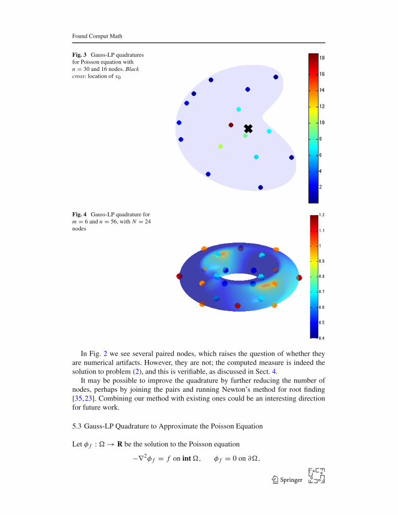
Fig. 3 Gauss-LP quadraturesfor Poisson equation withn = 30 and 16 nodes. Blackcross: location of x0

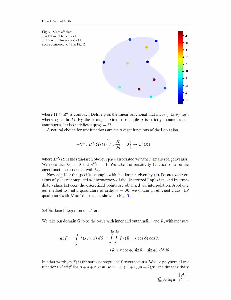
Fig. 4 Gauss-LP quadrature form = 6 and n = 56, with N = 24nodes

In Fig. 2 we see several paired nodes, which raises the question of whether theyare numerical artifacts. However, they are not; the computed measure is indeed thesolution to problem (2), and this is verifiable, as discussed in Sect. 4.

It may be possible to improve the quadrature by further reducing the number ofnodes, perhaps by joining the pairs and running Newton’s method for root finding[35,23]. Combining our method with existing ones could be an interesting directionfor future work.

5.3 Gauss-LP Quadrature to Approximate the Poisson Equation

Let φ f : " → R be the solution to the Poisson equation

−∇2φ f = f on int", φ f = 0 on ∂",

123

Found Comput Math

Fig. 5 Gauss-LP quadrature on 2D unit square with m = 6 and n = 21. The first quadrature uses 9 nodes,whereas the Gauss-LP quadrature produced with the rather odd choice of r uses only 8

123

Found Comput Math

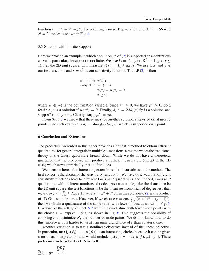
Fig. 6 More efficientquadrature obtained withdifferent r . This one uses 11nodes compared to 12 in Fig. 2

where ! ⊆ Rd is compact. Define q as the linear functional that maps f to φ f (x0),where x0 ∈ int!. By the strong maximum principle q is strictly monotone andcontinuous. It also satisfies supp q = !.

A natural choice for test functions are the n eigenfunctions of the Laplacian,

−∇2 : H2(!) ∩!

f : ∂ f∂"n

= 0#

→ L2(X),

where H2(!) is the standard Sobolev space associated with the n smallest eigenvalues.We note that λ0 = 0 and p(0) = 1. We take the sensitivity function r to be theeigenfunction associated with λn .

Now consider the specific example with the domain given by (4). Discretized ver-sions of p(i) are computed as eigenvectors of the discretized Laplacian, and interme-diate values between the discretized points are obtained via interpolation. Applyingour method to find a quadrature of order n = 30, we obtain an efficient Gauss-LPquadrature with N = 16 nodes, as shown in Fig. 3.

5.4 Surface Integration on a Torus

We take our domain! to be the torus with inner and outer radii r and R, with measure

q( f ) =$

!

f (x, y, z) d S =2π$

0

2π$

0

f ((R + r cosφ) cos θ,

(R + r cosφ) sin θ, r sin φ) dφdθ .

In other words, q( f ) is the surface integral of f over the torus. We use polynomial testfunctions x p yq zr for p + q + r < m, so n = m(m + 1)(m + 2)/6, and the sensitivity

123

Found Comput Math

function r = xm + ym + zm . The resulting Gauss-LP quadrature of order n = 56 withN = 24 nodes is shown in Fig. 4.

5.5 Solution with Infinite Support

Here we provide an example in which a solution µ⋆ of (2) is supported on a continuouscurve; in particular, the support is not finite. We take" = {(x, y) ∈ R2 : −1 ≤ x, y ≤1}, i.e., the 2D unit square, with measure q( f ) =

!" f dxdy. We use 1, x , and y as

our test functions and r = x2 as our sensitivity function. The LP (2) is then

minimize µ(x2)

subject to µ(1) = 4,

µ(x) = µ(y) = 0,

µ ≥ 0,

where µ ∈ M is the optimization variable. Since x2 ≥ 0, we have p⋆ ≥ 0. So afeasible µ is a solution if µ(x2) = 0. Finally, dµ⋆ = 2dδ0(x)dy is a solution andsupp µ⋆ is the y-axis. Clearly, |supp µ⋆| = ∞.

From Sect. 3 we know that there must be another solution supported on at most 3points. One such example is dµ = 4dδ0(x)dδ0(y), which is supported on 1 point.

6 Conclusion and Extensions

The procedure presented in this paper provides a heuristic method to obtain efficientquadratures for general integrals in multiple dimensions, a regime where the traditionaltheory of the Gauss quadrature breaks down. While we do not have a theoreticalguarantee that the procedure will produce an efficient quadrature (except in the 1Dcase) we observe empirically that it often does.

We mention here a few interesting extensions of and variations on the method. Thefirst concerns the choice of the sensitivity function r . We have observed that differentsensitivity functions lead to different Gauss-LP quadratures and, indeed, Gauss-LPquadratures with different numbers of nodes. As an example, take the domain to bethe 2D unit square, the test functions to be the bivariate monomials of degree less thanm, and q( f ) =

!" f dxdy. If we let r = xm+ym , then the solution to (2) is the product

of 1D Gauss quadratures. However, if we choose r = cos(π2"

(x + 1)2 + (y + 1)2),then we obtain a quadrature of the same order with fewer nodes, as shown in Fig. 5.Likewise, in the setting of Sect. 5.2 we find a quadrature with fewer node points withthe choice r = exp(x2 + y3), as shown in Fig. 6. This suggests the possiblity ofchoosing r to minimize N , the number of node points. We do not know how to dothis; moreover, it is harder to justify an unnatural choice of r than a natural one.

Another variation is to use a nonlinear objective instead of the linear objective.In particular, max{µ( f1), . . . , µ( fk)} is an interesting choice because it can be givena minimax interpretation and would include |µ( f )| = max{µ( f ), µ(− f )}. Theseproblems can be solved as LPs as well.

123

Found Comput Math

Finally, we could consider the extension to signed measures. For signed measures itmakes sense to use the objective ∥µ∥, which would be an infinite-dimensional analogof ℓ1 minimization.

Acknowledgments We thank Pablo Parrilo for helpful conversations; indeed, this paper grew out ofconversations with him. We also thank Paul Constantine for his helpful feedback. Ernest Ryu is supportedby the Department of Energy Office of Science Graduate Fellowship Program (DOE SCGF) and by theSimons Foundation.

Appendix 1: Notation

We write Cb for the Banach space of bounded continuous functions on ". Write∥ · ∥∞ : Cb → R for the supremum norm defined as

∥ f ∥∞def= sup

x∈"| f (x)|.

We write M for the Banach space of finite signed Borel measures on " and forµ ∈ M write µ ≥ 0 to denote that µ is unsigned. An unsigned measure µ is finite ifµ(") < ∞.

The support of µ ∈ M is defined as

supp µ = {x ∈ "|∀ r > 0, µ(B(x, r)) > 0} ,

and |supp µ| denotes the cardinality of supp µ as a set.We write N for the Banach space of normal signed Borel charges of bounded

variation. A charge is a set function defined on an algebra and is like a measureexcept that it is only finitely (and not necessarily countably) additive. A charge isBorel if it is defined on the algebra generated by open sets. A charge is normal ifµ(A) = sup{µ(F) : F ⊆ A, F closed} = inf{µ(G) : A ⊆ G, G open}. A charge istight if µ(A) = sup{µ(K ) : K ⊆ A, K compact}. For µ ∈ M write µ ≥ 0 to denotethat µ is unsigned. An unsigned charge µ is of bounded variation if µ(") < ∞.Integration with respect to a charge is defined similarly to Lebesgue integration [2,§14.2].

By Theorem 5, N is isomorphic to the dual of Cb. Thus, for any µ ∈ N and f ∈ Cbwe can view µ as a linear functional acting on f , and we denote this action as

⟨ f, µ⟩ def=!

"

f dµ.

Appendix 2: Miscellaneous Theorems

Theorem 3 If supp q = ", a Gauss quadrature is the only quadrature that integrates1, x, . . . , xn−1 exactly with n/2 or fewer nodes [31].

123

Found Comput Math

Theorem 4 On ! ⊆ Rd , every tight finite Borel charge is a measure [2, §12.1].(Precisely speaking, the charge has a unique extension to the Borel σ -algebra that isa measure.)

In the proof of strong duality we will encounter charges, which are generalizations ofmeasures. Fortunately, Theorem 4 will allow us to conclude that the charge is in facta measure.

Theorem 5 For a domain! not necessarily compact, the dual space C∗b is isomorphic

to N , the space of signed normal Borel charges of bounded variation [2, §14.3].

Theorem 5, used in the proof of Theorem 1, is analogous to the Riesz–Markov theoremand provides an explicit representation of the dual space C∗

b .

Appendix 3: Proof of Main Results

Appendix 3.1: Proof of Theorem 1

We will call the optimization problem (1) the primal problem and the following prob-lem the dual problem.

maximizen−1!i=0

νi+1⟨xi , q⟩

subject to λ = xn −n−1!i=0

νi+1xi ,

λ(x) ≥ 0, for all x ∈ !,

(5)

where ν ∈ Rn is the optimization variable. We define µ⋆ and ν⋆ as solutions of the pri-mal and dual problems, respectively. We write λ⋆ for the polynomial that correspondsto ν⋆. Let p⋆ and d⋆ denote the optimal values of the primal and dual problems.

In the proof we first introduce a new LP, problem (6), that is similar to the original LP,problem (1), but different in that is has a larger search space. We show that problem (6)is the dual of problem (5) and that strong duality and complementary slackness holds.The nonnegative polynomial λ⋆ can have at most n/2 roots, and this will allow us toconclude that in fact problems (6) and (1) must share the same solution and that thesolution must be a Gauss quadrature.

Proof Define

ψ(x) ="

1 if |x | ≤ 11

xn otherwise

and the norm

∥ f ∥∞,ψ = ∥ fψ∥∞ = supx∈!

| f (x)ψ(x)|.

123

Found Comput Math

Let D be the set of continuous real-valued functions f defined on ! such that∥ f ∥∞,ψ < ∞. In other words, D = 1

ψCb is the space of continuous functionsthat grow at a rate of at most O(xn).

The map T : D → Cb, where T : f $→ fψ , is an isometric lattice isomorphismbetween (D, ∥·∥∞,ψ ) and (Cb, ∥·∥∞) [2, §14.3]. Thus, (D, ∥·∥∞,ψ ) is a Banach space.Moreover, since C∗

b∼= N by Theorem 5, the isomorphism tells us that D∗ ∼= ψN ,

where N is the Banach space of normal Borel charges of bounded variation.Consider the following variant of the primal problem: (1)

minimize ⟨xn, µ⟩subject to ⟨xi , µ⟩ = ⟨xi , q⟩, i = 0, . . . , n − 1,

µ ≥ 0, (6)

where µ ∈ ψN ∼= D∗ is the optimization variable. Note that µ, which used to be inM, now resides in a larger space. Weak duality between (6) and (5) can be readilyshown via standard arguments. Both primal and dual problems are feasible becauseµ = q and ν = 0 are feasible points, and therefore −∞ < d⋆ ≤ p⋆ < ∞.

Now we can apply Lagrange duality, which states: if d⋆ is finite (which we haveshown) and if there is a strictly feasible ν, then strong duality holds, a primal solutionexists, and complementary slackness holds [21, §8.6]. The point ν = e1 is strictlyfeasible, and this establishes strong duality and the existence of a primal solution µ⋆.

We now claim that the dual problem attains the supremum, i.e., a solution ν⋆ exists.We prove this in Appendix 3.2.

Next we will show that µ⋆ is a measure (not just a charge) and that supp µ⋆ ⊆{x1, x2, . . . , xk}, where x1, x2, . . . , xk are the roots of the polynomial λ⋆. Comple-mentary slackness states that ⟨µ⋆, λ⋆⟩ = 0. Remember that λ⋆ ≥ 0 by definition. Forany set A ⊆ R\!k

i=1 B(xi , ε), where ε > 0 is small, there exists a small enoughδ > 0 such that δ1A ≤ λ⋆, where 1A is the indicator function, and we have

δµ⋆(A) ="

!

δ1A dµ⋆ ≤"

!

λ⋆ dµ⋆ = 0.

So we conclude µ⋆(A) = 0. Now by the normality of the charge µ⋆,

µ⋆((xi − ε, xi )) = sup{µ⋆(F) : F closed and F ⊆ (xi − ε, xi )}.

However, by the previous argument, µ⋆(F) = 0 for any closed F such that F ⊆(xi−ε, xi ). Therefore,µ⋆((xi−ε, xi )) = 0 and, by the same logic,µ⋆((xi , xi+ε)) = 0.Thus, µ⋆(R\{x1, x2, . . . , xk}) = 0, and for any measurable set A we have µ⋆(A) =µ⋆(A∩{x1, x2, . . . , xk}). In particular, {x1, x2, . . . , xk} is compact, and this establishesthe tightness of µ⋆. Thus, by Theorem 4, we conclude that µ⋆ is a discrete measureand can have point masses only at x1, x2, . . . , xk .

Since µ⋆ is a discrete measure,

µ⋆ ∈ {µ ∈ M|µ is feasible for the primal problem (1)} ⊆ ψN .

123

Found Comput Math

Therefore, the primal problem can be simplified by searching over the feasible mea-sures in M and not over the entire superspace ψN . In other words, µ⋆, the solutionto problem (6), is a solution to the original problem (1).

Moreover, since λ⋆ is a nonnegative polynomial of degree n, it can have at most n/2distinct roots in$, and therefore |supp µ⋆| ≤ n/2. In other words, µ⋆ is equivalent toa quadrature that integrates 1, x, x2, . . . , xn−1 exactly with n/2 or fewer nodes. Thus,by Theorem 3, we conclude that µ⋆ must be the Gauss quadrature and that the solutionµ⋆ is unique. ⊓$

Appendix 3.2: Attainment of Dual Optimum

Lemma 1 Let K ⊆ Rn be a proper cone. Assume u0 ∈ K ∗ has the property that forany v ∈ K we have vT u0 > 0, unless v = 0. Then u0 ∈ int (K ∗).

Proof Assume for contradiction that u0 ∈ ∂K ∗. Then there exists a nonzero separatinghyperplane λ such that λT u0 = 0 and λT u ≥ 0 for any u ∈ K ∗. However, this impliesthat λ ∈ K ∗∗ = K , and this contradicts the assumption that vT u0 > 0 for any nonzerov ∈ K . Thus we conclude that u0 ∈ int (K ∗). ⊓$

Theorem 6 A solution to the dual problem (5) is attained.

Proof Let K be the convex cone defined as

K = {y ∈ Rn+1|yn+1xn + yn xn−1 + · · · + y2x + y1 ≥ 0 for x ∈ $},

i.e., the cone of coefficients of nonnegative polynomials.Also, let M be the convex cone defined as

M = {m ∈ Rn+1 : m =!⟨1, µ⟩, ⟨x, µ⟩, . . . , ⟨xn−1, µ⟩, ⟨xn, µ⟩

", µ ≥ 0}, (7)

i.e., the cone of possible moments. We note that K ∗ = cl M , where cl M denotes theclosure of M , and that K ∗∗ = K as K is a proper cone [5, pp. 65–66]. The followingduality argument hinges on these facts.

Let m0 ∈ Rn+1 be the moment vector, i.e., (m0)i+1 = q(xi ) for i = 0, . . . , n.Consider the following problem:

minimize xn+1

subject to xi = (m0)i , i = 1, . . . , n,

x ∈ K ∗, (8)

where x ∈ Rn+1 is the optimization variable. (Since K ∗ = cl M , problem (8) is infact equivalent to problem (1).) Lagrange duality tells us that the dual of (8) is (5)and that a dual solution ν⋆ exists if (8) has a strictly feasible point (i.e., if Slater’sconstrain qualification holds) [5, §5.3]. We omit the Lagrange dual derivation becauseit is routine and involves no unexpected tricks.

123

Found Comput Math

Consider any y ∈ K such that y = 0. Then

yT m0 =!

!

n"

i=0

yi+1xi dq > 0

since by definition y ∈ K implies#n

i=0 yi+1xi ≥ 0 and since supp q = !. Thus, byLemma 1, we see that m0 ∈ int (K ∗), i.e., m0 is strictly feasible. Hence, we concludethat a dual solution ν⋆ exists. ⊓&

Appendix 3.3: Proof of Theorem 2

Proof We write

M = {m ∈ Rn+1 : m =$⟨p(0), µ⟩, ⟨p(1), µ⟩, . . . , ⟨p(n−1), µ⟩, ⟨r, µ⟩

%, µ ≥ 0},

(9)

and we will call M the moment cone. Also, define

K =&(p(0)(x), p(1)(x), . . . , p(n−1)(x), r(x)) ∈ Rn+1 : x ∈ !

'.

Since the p(i) and r are continuous, K is the image of a compact set under a continuousfunction and therefore is compact. We assume as before that p(0) = 1 and, therefore,0 /∈ convK , where convK denotes the convex hull of K . Therefore, cone K , theconical hull of K , is closed [16, §1.4].

Now we prove cone K = M . By choosing µ to have point masses at a finite numberof points in (9), we can produce any element in cone K and therefore cone K ⊆ M .Now assume for contradiction that cone K = M . In other words, assume there existsan m ∈ M such that m /∈ cone K . Since cone K is a closed convex set, there must be astrictly separating hyperplane λ such that λT m < 0 and λT n ≥ 0 for any n ∈ cone K .However, since m ∈ M , there must exist a corresponding measure µ ≥ 0 that producedm in (9), i.e.,

mi+1 = ⟨p(i), µ⟩ for i = 0, . . . , n − 1 and mn+1 = ⟨r, µ⟩.

Therefore,

λT m =(

λn+1r +n−1"

i=0

λi+1 p(i), µ

)

< 0,

and this in particular implies that

λn+1r(x) +n−1"

i=0

λi+1 p(i)(x) < 0

123

Found Comput Math

for some x ∈ !. However, since by construction λT n ≥ 0 for all n ∈ K ⊆ cone K ,i.e.,

λn+1r(x) +n−1!

i=0

λi+1 p(i)(x) ≥ 0 for all x ∈ !,

we have a contradiction. Therefore, cone K = M and M is closed.Now consider the optimization problem

minimize mn+1

subject to mi = q(p(i)), i = 0, . . . , n − 1,

m ∈ M,

where m ∈ Rn+1 is the optimization variable. Note that this problem is equivalentto the original problem (2). Since M is closed, so is the feasible set. Moreover, thefeasible set is bounded because for any m ∈ M , the last coordinate mn+1 (the onlyone that is not fixed) is bouned since

|mn+1| = |µ(r)| ≤ ∥r∥∞µ(1) = ∥r∥∞q(1) < ∞

for some nonnegative measure µ ∈ M. Therefore, the feasible set is compact. Finally,the feasible set is nonempty because m ∈ M generated by the measure q is a feasiblepoint. Therefore, there exist an optimal m⋆ for the reduced problem and a µ⋆ thatgenerated m⋆; this µ⋆ is optimal for the original problem (2).

Now, by Carathéodory’s theorem on cones [29, §17], m⋆ ∈ cone K = M can beexpressed as a linear combination of at most n+1 vectors in K . This linear combinationis equivalent to a measure with point masses at at most n +1 locations. In other words,m⋆ can be produced (in the sense of (9)) by a measure µ⋆, where |supp µ⋆| ≤ n + 1.This µ⋆ is a solution to problem (2).

Finally, we can further reduce the support of this solution. Given a solution µ⋆ withfinite support, we can restrict problem (2) to searching only over measures that aresupported on supp µ⋆. This reduces problem (2) to a finite-dimensional LP, whichalways has a solution supported on n or fewer points [22, §2.4]. ⊓)

References

1. M. Abramowitz and I. Stegun. Handbook of Mathematical Functions, With Formulas, Graphs, andMathematical Tables. Dover Publications, Incorporated, New York, 1964.

2. C. Aliprantis and K. Border. Infinite Dimensional Analysis: A Hitchhiker’s Guide. Springer, New York,3rd edition, 2006.

3. E. Anderson and P. Nash. Linear Programming in Infinite-dimensional Spaces: Theory and Applica-tions. Wiley, New York, 1987.

4. E. Anderson and A. Philpott. Infinite Programming: Proceedings of an International Symposium onInfinite Dimensional Linear Programming, Churchill College, Cambridge, United Kingdom, September7–10, 1984. Springer-Verlag, New York, 1985.

5. S. Boyd and L. Vandenberghe. Convex Optimization. Cambridge University Press, Cambridge, 2004.

123

Found Comput Math

6. E. Candes, J. Romberg, and T. Tao. Robust uncertainty principles: Exact signal reconstruction fromhighly incomplete frequency information. IEEE Transactions on Information Theory, 52(2):489–509,2006.

7. S. Chen, D. Donoho, and M. Saunders. Atomic decomposition by basis pursuit. SIAM Journal onScientific Computing, 20(1):33–61, 1999.

8. P. Davis. A construction of nonnegative approximate quadratures. Mathematics of Computation,21(100):578–582, 1967.

9. P. Davis and P. Rabinowitz. Methods of Numerical Integration. Academic Press, Orlando, 2nd edition,1984.

10. A Fiacco and K. Kortanek. Semi-infinite Programming and Applications: An International Symposium,Austin, Texas, September 8–10, 1981. Springer-Verlag, New York, 1983.

11. C. Gauss. Methodus nova integralium valores per approximationem inveniendi. Commentationes Soci-etatis Regiae Scientarium Gottingensis Recentiores, 3:39–76, 1814.

12. A. Glaser, X. Liu, and V. Rokhlin. A fast algorithm for the calculation of the roots of special functions.SIAM Journal on Scientific Computing, 29(4):1420–1438, 2007.

13. M. Goberna and M. López. Linear Semi-infinite Optimization. John Wiley, 1998.14. G. Golub and J. Welsch. Calculation of gauss quadrature rules. Mathematics of Computation,

23(106):221–230, 1969.15. P. Hammer and A. Stroud. Numerical evaluation of multiple integrals II. Mathematics of Computation,

12:272–280, 1958.16. J. Hiriart-Urruty and C. Lemarechal. Convex Analysis and Minimization Algorithms I: Fundamentals.

Springer, New York, October 1993.17. S. Karlin and W. Studden. Tchebycheff Systems: With Applications in Analysis and Statistics. Inter-

science Publishers, New York, 1966.18. M. Krein. The ideas of P. L. Chebyshev and A. A. Markov in the theory of limiting values of integrals

and their further development. American Mathematical Society Translations (Series 2), 12:1–122,1959.

19. V. Krylov. Approximate Calculation of Integrals. Macmillan, New York, 1962.20. J. Lasserre. Global optimization with polynomials and the problem of moments. SIAM Journal on

Optimization, 11:796–817, 2001.21. D. Luenberger. Optimization by Vector Space Methods. John Wiley & Sons, New York, 1967.22. D. Luenberger and Y. Ye. Linear and Nonlinear Programming. Springer, New York, third edition,

2008.23. J. Ma, V. Rokhlin, and S. Wandzura. Generalized Gaussian quadrature rules for systems of arbitrary

functions. SIAM Journal on Numerical Analysis, 33(3):971–996, 1996.24. A. Markov. On the limiting values of integrals in connection with interpolation. Zapiski Imperatorskoj

Akademii Nauk po Fiziko-matematiceskomu Otdeleniju, 5:146–230, 1898.25. G. Murty and S. Kabadi. Some NP-complete problems in quadratic and nonlinear programming.

Mathematical Programming, 39(2):117–129, 1987.26. J. Nocedal and S. Wright. Numerical Optimization. Springer, New York, 2nd edition, 2006.27. W. Peirce. Numerical integration over the planar annulus. Journal of the Society for Industrial and

Applied Mathematics, 5(2):66–73, 1957.28. J. Powell. Approximation Theory and Methods. Cambridge University Press, Cambridge, 1981.29. R. Rockafellar. Convex Analysis. Princeton University Press, Princeton, 1996.30. A. Stroud. Quadrature methods for functions of more than one variable. Annals of the New York

Academy of Sciences, 86(3):776–791, 1960.31. A. Stroud and D. Secrest. Gaussian Quadrature Formulas. Prentice-Hall, Englewood Cliffs, 1966.32. E. Süli and D. Mayers. An Introduction to Numerical Analysis. Cambridge University Press, Cambridge,

2003.33. R. Tibshirani. Regression shrinkage and selection via the lasso. Journal of the Royal Statistical Society

(Series B), 58:267–288, 1996.34. B. Vioreanu. Spectra of Multiplication Operators as a Numerical Tool. PhD thesis, Yale University,

2012.35. H. Xiao and Z. Gimbutas. A numerical algorithm for the construction of efficient quadrature rules in

two and higher gimensions. Computational Mathematics with Applications, 59(2), 2010.

123